AN INTEGRATED EARTHQUAKE IMPACT ASSESSMENT...
224
AN INTEGRATED EARTHQUAKE IMPACT ASSESSMENT SYSTEM Report No. 11-02 Sheng-Lin Lin Amr S. Elnashai Billie F. Spencer, Jr. Youssef M. A. Hashash Larry A. Fahnestock May 2011
Transcript of AN INTEGRATED EARTHQUAKE IMPACT ASSESSMENT...

AN INTEGRATED EARTHQUAKE IMPACT ASSESSMENT SYSTEM
Report No. 11-02
Sheng-Lin Lin Amr S. Elnashai
Billie F. Spencer, Jr. Youssef M. A. Hashash
Larry A. Fahnestock
May 2011

ii
ABSTRACT
This report presents a methodology for the refined, reliable, integrated and
versatile assessment of the impact of earthquakes on civil infrastructure systems by using
free-field and structural instrumentation as well as hybrid simulation. The methodology is
presented through a seamlessly-integrated, transparent, transferable and extensible
software platform, referred to as NEES Integrated Seismic Risk Assessment Framework
(NISRAF). The software tool combines all necessary components in order to obtain the
most reliable earthquake impact assessment results possible. The components are (i)
hybrid simulation, (ii) free-field and (iii) structural sensor measurements, (iv) hazard
characterization, (v) system identification-based model updating, (vi) hybrid fragility
analysis and (vii) impact assessment software.
NISRAF has been built and demonstrated via applications to an actual test bed in
the Los Angeles area. Based on an instrumented six-story steel moment resisting frame
building and free-field station records, site response analysis was performed, and hazard
characterization and surface ground motion records were generated for further use during
the hybrid simulations and fragility analyses. Meanwhile, the finite element model was
built, and the natural frequencies and mode shapes were identified using suitable
algorithms. The numerical model was updated through a sensitivity-based model
updating technique. Next, hybrid simulations—with the most critical component of the
structural system tested in the laboratory and the remainders of the structure simulated
analytically—were conducted within UI-SIMCOR and ZEUS-NL, both software
iii
platforms of the University of Illinois. The simulated results closely matched their
measured counterparts. Fragility curves were derived using hybrid simulation results
along with dispersions from research on similar structures from the literature. Impact
assessment results using the generated hazard map and fragility curves correlated very
well with field observations following the Northridge earthquake of 17 January 1994.
The novelty of the developed framework is primarily the improvement of every
component of earthquake impact assessment and the integration of these components—
most of which have not been deployed in such an application before—into a single
versatile and extensible platform. To achieve seamless integration and to arrive at an
operational and verified system, several components were used innovatively, tailored to
perform the role required by NISRAF. The integrated feature brings the most advanced
tools of earthquake hazard and structural reliability analyses into the context of societal
requirement for accurate evaluation of the impact of earthquakes on the built environment.

iv
ACKNOWLEDGMENTS
The work was financially supported by the NEESR-SD project, Framework for
Development of Hybrid Simulation in an Earthquake Impact Assessment Context, funded
by the National Science Foundation (NSF) under award number 0724172. I must also
acknowledge the financial and logistical contributions of the Mid-America Earthquake
(MAE) Center, a NSF Engineering Research Center funded under grant EEC-9701785.

v
TABLE OF CONTENTS LIST OF TABLES ..................................................................................................................................... X�
LIST OF FIGURES .................................................................................................................................. XI�
CHAPTER 1 ................................................................................................................................................ 1�
1.1 Background ......................................................................................................................................... 1�
1.2 Objective and Scope ........................................................................................................................... 5�
1.3 Organization of Dissertation ............................................................................................................... 7�
CHAPTER 2 ................................................................................................................................................ 9�
2.1 Introduction ......................................................................................................................................... 9�
2.2 Free-Field and Structural Instrumentation .......................................................................................... 9�
2.2.1 ANSS, Advanced National Seismic System .............................................................................. 10�
2.2.2 COSMOS, the Consortium of Organizations for Strong Motion Observation Systems ............ 11�
2.2.3 CESMD, Center for Engineering Strong Motion Data .............................................................. 11�
2.2.4 Pacific Earthquake Engineering Research Center (PEER) NGA Database ............................... 12�
2.2.5 CSMIP, California Strong Motion Instrumentation Program .................................................... 12�
2.3 Seismic Hazard Characterization ...................................................................................................... 13�
2.3.1 Attenuation Relationship............................................................................................................ 14�
2.3.2 Synthetic Ground Motions Generation ...................................................................................... 18�
2.3.3 Site Response Analysis .............................................................................................................. 19�
2.3.3.1 SHAKE91 ........................................................................................................................... 21�
2.3.3.2 DEEPSOIL .......................................................................................................................... 22�
2.4 Model Calibration ............................................................................................................................. 23�
2.4.1 System Identification ................................................................................................................. 23�
2.4.2 Model Updating ......................................................................................................................... 24�
2.5 Dynamic Response Simulation of Structures .................................................................................... 25�
2.5.1 Model Analytical Simulation ..................................................................................................... 25�
2.5.2 PSD, Pseudo-Dynamic Test ....................................................................................................... 26�
2.5.3 Hybrid Simulation ...................................................................................................................... 26�
2.6 Fragility Analysis .............................................................................................................................. 28�
2.7 Earthquake Impact Assessment Tools .............................................................................................. 29�
2.7.1 MAEviz ...................................................................................................................................... 31�
2.7.2 HAZUS-MH .............................................................................................................................. 32�

vi
2.8 Summary and Discussion .................................................................................................................. 33�
CHAPTER 3 .............................................................................................................................................. 35�
3.1 Introduction ....................................................................................................................................... 35�
3.2 Overview of the Advanced Hazard Characterization Analysis Method ........................................... 36�
3.3 Seismic Hazard Analysis .................................................................................................................. 37�
3.3.1 Seismic Hazard Analysis from Natural Records ........................................................................ 37�
3.3.2 Seismic Hazard Analysis for Scenario Earthquakes .................................................................. 40�
3.3.2.1 Significant duration prediction equation ............................................................................. 41�
3.3.2.2 Deaggregation results from Probabilistic Seismic Hazard Analysis ................................... 43�
3.4 Synthetic Ground Motion Generation ............................................................................................... 44�
3.4.1 Intensity Function ...................................................................................................................... 45�
3.4.2 Duration Parameters ................................................................................................................... 46�
3.5 Site Response Analysis ..................................................................................................................... 47�
3.6 Hazard Map Generation .................................................................................................................... 48�
3.7 Verification Studies .......................................................................................................................... 49�
3.7.1 Introduction ................................................................................................................................ 49�
3.7.2 Hazard Models Calibrated with Measured Records ................................................................... 52�
3.7.3 Application Examples ................................................................................................................ 58�
3.7.3.1 Application 1—synthetic ground motions through the Northridge earthquake mechanism ........................................................................................................................................................ 59�
3.7.3.2 Application 2—synthetic ground motions with various hazard levels................................ 64�
3.7.3.3 Application 3— a site specific hazard map under the Northridge earthquake in LA area .. 68�
3.8 Summary and Discussion .................................................................................................................. 74�
CHAPTER 4 .............................................................................................................................................. 75�
4.1 Introduction ....................................................................................................................................... 75�
4.2 Overview of the Advanced Hybrid Fragility Analysis Method ........................................................ 76�
4.3 Verification Studies .......................................................................................................................... 77�
4.3.1 Structural Model and Seismic Input ........................................................................................... 78�
4.3.1.1 Building Description and Structural Model ........................................................................ 78�
4.3.1.2 Performance Limit State ..................................................................................................... 79�
4.3.1.3 Seismic Input ...................................................................................................................... 79�
vii
4.3.2 Hybrid Simulation ...................................................................................................................... 79�
4.3.2.1 Testing Facility ................................................................................................................... 80�
4.3.2.2 Specimen Design................................................................................................................. 82�
4.3.2.3 Software Environment ........................................................................................................ 84�
4.3.2.4 Experimental Setup ............................................................................................................. 86�
4.3.2.5 Hybrid Simulation Results .................................................................................................. 88�
4.3.3 Hybrid Fragility Analysis........................................................................................................... 90�
4.3.3.1 Mean PGA Values from Hybrid Simulation ....................................................................... 90�
4.3.3.2 Dispersions from Literature ................................................................................................ 95�
4.3.3.3 Hybrid Fragility Curves ...................................................................................................... 97�
4.4 Fragility Relationships for Other Building Types ............................................................................. 99�
4.4.1 Parameterized Fragility Method ................................................................................................. 99�
4.4.2 Fragility Relationships for Los Angeles area ........................................................................... 100�
4.5 Summary and Discussion ................................................................................................................ 103�
CHAPTER 5 ............................................................................................................................................ 104�
5.1 Introduction ..................................................................................................................................... 104�
5.2 Architecture of NISRAF ................................................................................................................. 104�
5.2.1 File Menu ................................................................................................................................. 108�
5.2.2 Strong Motion Menu ................................................................................................................ 108�
5.2.3 Hazard Characterization Menu ................................................................................................ 110�
5.2.3.1 Seismic Hazard Analysis .................................................................................................. 111�
5.2.3.2 Synthetic Time Histories ................................................................................................... 113�
5.2.3.3 Hazard Map Generation .................................................................................................... 116�
5.2.4 Structural Model Menu ............................................................................................................ 118�
5.2.5 Model Calibration Menu .......................................................................................................... 120�
5.2.6 Hybrid Simulation Menu ......................................................................................................... 122�
5.2.7 Fragility Analysis Menu........................................................................................................... 124�
5.2.8 Impact Assessment Menu ........................................................................................................ 128�
5.2.9 Help Menu ............................................................................................................................... 129�
5.3 Communication Protocols and Analysis Platforms ......................................................................... 129�

viii
5.4 Features of NISRAF ....................................................................................................................... 130�
5.5 Potentials, Limitations and Challenges ........................................................................................... 132�
CHAPTER 6 ............................................................................................................................................ 133�
6.1 Introduction ..................................................................................................................................... 133�
6.2 Application 1: A 6-Story Steel Building in Burbank, California .................................................... 133�
6.2.1 Introduction .............................................................................................................................. 134�
6.2.1.1 Building Information ......................................................................................................... 134�
6.2.1.2 Site Condition ................................................................................................................... 136�
6.2.2 Strong Motion .......................................................................................................................... 136�
6.2.3 Hazard Characterization ........................................................................................................... 137�
6.2.4 Structural Model ...................................................................................................................... 138�
6.2.5 Model Calibration .................................................................................................................... 139�
6.2.5.1 System Identification ........................................................................................................ 139�
6.2.5.2 Model Updating ................................................................................................................ 142�
6.2.6 Hybrid Simulation & Fragility Analysis .................................................................................. 144�
6.2.7 Impact Assessment ................................................................................................................... 144�
6.3 Application 2: the Los Angeles area earthquake impact assessment .............................................. 147�
6.3.1 Introduction .............................................................................................................................. 147�
6.3.2 Assessment Results and Comparison ....................................................................................... 147�
6.4 Uncertainty Analysis in NISRAF ................................................................................................... 149�
6.4.1 Introduction .............................................................................................................................. 149�
6.4.2 Methodology of uncertainty analysis in MAEviz .................................................................... 151�
6.4.2.1 Uncertainty in hazard ........................................................................................................ 152�
6.4.2.2 Uncertainty in structural damage ratio .............................................................................. 153�
6.4.2.3 Uncertainty in nonstructural and content damage ratio .................................................... 155�
6.4.2.4 Loss estimation ................................................................................................................. 155�
6.4.2.5 Uncertainty representation ................................................................................................ 156�
6.4.3 Uncertainty analysis in NISRAF .............................................................................................. 156�
6.4.4 Discussion of Uncertainty Analysis ......................................................................................... 157�
6.5 Summary and Conclusion ............................................................................................................... 158�
CHAPTER 7 ............................................................................................................................................ 160�

ix
7.1 Summary of Findings ...................................................................................................................... 160�
7.2 Ideas for Future Research ............................................................................................................... 162�
7.3 Closure ............................................................................................................................................ 164�
REFERENCES ........................................................................................................................................ 166�
APPENDIX A .......................................................................................................................................... 174�
APPENDIX B .......................................................................................................................................... 186�
APPENDIX C .......................................................................................................................................... 204�
C.1 Structural Parameters for PFM ....................................................................................................... 204�
C.2 Earthquake Demand ....................................................................................................................... 204�
C.3 Fragility Relationships ................................................................................................................... 204�
APPENDIX D .......................................................................................................................................... 207�
D.1 System Identification ..................................................................................................................... 207�
D.2 Model Updating ............................................................................................................................. 210�

x
LIST OF TABLES Table 3-1 Soil properties of Burbank site (Fumal et al., 1979) .................................................................. 50�Table 3-2 Seismic parameters of the 1994 Northridge earthquake (USGS, 1996) .................................... 53�Table 3-3 Parameters from SMIP report required for the CB-NGA model ............................................... 54�Table 3-4 ����, ���� and ���� values of stations close to the borehole site .............................................. 56�Table 3-5 ����, ���� and ���� values after modification .......................................................................... 56�Table 3-6 Comparison between the measured and predicted seismic parameters ..................................... 60�Table 3-7 Deaggregation results at Burbank site ....................................................................................... 65�Table 3-8 Contributed fault information based on deaggregation results .................................................. 65�Table 3-9 Comparisons of PGA value between the measured and the calculated ..................................... 74�Table 4-1 Force and displacement capacities of portable LBCB (Holub, 2010) ....................................... 81�Table 4-2 Scale factor for design small scale specimen ............................................................................. 83�Table 4-3 Dimension and material properties of real column and small-scale specimen .......................... 83�Table 4-4 Interstory drift angle (target ISDA) and PGA from hybrid simulation tests .............................. 92�Table 4-5 Logarithmic uncertainties for mid-rise building (FEMA, 2000a) .............................................. 96�Table 4-6 Mean PGA value and dispersions for mid-rise steel building fragility curves .......................... 97�Table 6-1 Frequency and � of identified with ERA method .................................................................... 140�Table 6-2 Selected parameters for model updating and updated results .................................................. 142�Table 6-3 Comparison of frequency and mode shape between the original and updated ........................ 143�Table 6-4 Comparison between impact assessment results ...................................................................... 145�Table 6-5 ATC-38 post-earthquake report for the Northridge earthquake of 1994 ................................. 145�Table 6-6 Comparison between NISRAF and MAEviz default ............................................................... 146�Table 6-7 Direct economic building loss ................................................................................................. 148�Table 6-8 Probability model for structural damage ratio (Bai et al., 2009) ............................................. 154�

xi
LIST OF FIGURES Figure 1-1 Devastating earthquakes in recent decades ................................................................................ 2�Figure 1-2 Schematic of the proposed integrated framework ...................................................................... 5�Figure 2-1 Source-to-site distances ............................................................................................................ 18�Figure 2-2 Average normalized response spectra (5% damping) for different local site condition ........... 21�Figure 3-1 Methodology and procedures of hazard characterization analysis ........................................... 36�Figure 3-2 Measured structures with instruments on the ground ............................................................... 38�Figure 3-3 Free-field records on an outcrop............................................................................................... 39�Figure 3-4 Free-field station record on soil surface ................................................................................... 39�Figure 3-5 Variation of bracketed duration (0.05g threshold) with magnitude and epicentral distance .... 42�Figure 3-6 Intensity functions implemented in SIMQKE (Gasparini and Vanmarcke, 1976) ................... 46�Figure 3-7 Definition of Tb and Ttotal .......................................................................................................... 46�Figure 3-8 Borehole log of the Burbank site (adapted from Fumal et al., 1979) ....................................... 51�Figure 3-9 Free-field and structural instruments around the Burbank site (CESMD) ............................... 52�Figure 3-10 Portrayed buried fault plane of the Northridge earthquake (USGS, 1996) ............................ 53�Figure 3-11 Comparison of the difference using different �� and ���� .............................................. 55�Figure 3-12 Difference when assuming ���� � � � for all the borehole sites ........................................ 57�Figure 3-13 Difference when using ���� value from PEER NGA Database ............................................. 57�Figure 3-14 Sensitivity of shear-wave velocity to the PGA predicted by CB-NGA ................................. 58�Figure 3-15 Response spectra generated through CB-NGA model ........................................................... 60�Figure 3-16 Synthetic ground motion with different duration and PGA ................................................... 61�Figure 3-17 Comparison between the natural and synthetic record ........................................................... 62�Figure 3-18 Comparison of response spectra ............................................................................................. 62�Figure 3-19 Comparison of response spectra with site response analysis (SR) ......................................... 64�Figure 3-20 Synthetic ground motions for different hazard level and duration ......................................... 66�Figure 3-21 Response spectra for different hazard level ............................................................................ 67�Figure 3-22 Locations of boreholes (black cross) in the SMIP geotechnical report .................................. 69�Figure 3-23 Subdivided areas and the selected boreholes in the Los Angeles area ................................... 69�Figure 3-24 Map of PGA for the 1994 Northridge earthquake in the Los Angeles area ........................... 70�Figure 3-25 ShakeMap for the 1994 Northridge earthquake (USGS)........................................................ 71�Figure 3-26 Hazard and difference of PGA between NISRAF and measured one .................................... 73�Figure 3-27 Hazard and difference of PGA between MAEviz and measured one .................................... 73�Figure 4-1 Flow chart for the advanced hybrid fragility analysis .............................................................. 77�Figure 4-2 Analytical model configuration for Burbank building ............................................................. 78�Figure 4-3 Hybrid simulation with two sub-structures (column and frame) .............................................. 80�Figure 4-4 Portable LBCB at MUST-SIM 1/5th-scale model laboratory ................................................... 81�Figure 4-5 Aluminum column specimen elevation, unit: in. ...................................................................... 83�Figure 4-6 Completed small-scale specimen ............................................................................................. 84�Figure 4-7 Small-scale experimental setup ................................................................................................ 87�Figure 4-8 Ground motion record of the 1994 Northridge earthquake (CSMIP # 24370) ......................... 89�Figure 4-9 Comparison of the roof drift between the measured and the hybrid simulation ...................... 89�Figure 4-10 Methodology and procedures for the advanced hybrid fragility analysis .............................. 91�Figure 4-11 Number of hybrid simulation tests to derive fragility curves ................................................. 92�

xii
Figure 4-12 Synthetic Ground motion (2% PE/50yrs with scale factor = 3.54) ........................................ 93�Figure 4-13 Comparison of column response between hybrid and multiplatform simulation ................... 93�Figure 4-14 Comparison of displacement between hybrid and multiplatform simulation ......................... 94�Figure 4-15 Comparison of displacement between hybrid and multiplatform simulation ......................... 94�Figure 4-16 Hybrid fragility curves for mid-rise steel moment resisting frame building in LA area ........ 97�Figure 4-17 Fragility relationship comparison between NISRAF and MAEviz ........................................ 98�Figure 4-18 Comparison of S1M (High-Code) fragility relationships ..................................................... 101�Figure 4-19 W1 (High-Code) fragility relationships comparison between PFM and MAEviz ............... 102�Figure 4-20 URMM (Pre-Code) fragility relationships comparison between PFM and MAEviz ........... 102�Figure 5-1 Architecture of NISRAF ........................................................................................................ 105�Figure 5-2 Welcome window and main window of NISRAF .................................................................. 107�Figure 5-3 File submenus in NISRAF ..................................................................................................... 108�Figure 5-4 Schematic of Strong Motion menu in NISRAF ...................................................................... 109�Figure 5-5 Strong Motion menu in NISRAF ........................................................................................... 109�Figure 5-6 Strong motion data GUI in Strong Motion menu ................................................................... 110�Figure 5-7 Hazard Characterization submenu in NISRAF ...................................................................... 111�Figure 5-8 Seismic hazard analysis GUI in Hazard Characterization menu ............................................ 112�Figure 5-9 Time history and response spectrum checking GUI ............................................................... 112�Figure 5-10 Define soil profiles and material properties GUI in NISRAF .............................................. 113�Figure 5-11 GUI to define seismic parameters ........................................................................................ 114�Figure 5-12 GUI to customize synthetic time history .............................................................................. 114�Figure 5-13 GUI to show analysis progress and response spectrum ........................................................ 115�Figure 5-14 Suites of generated synthetic time histories ......................................................................... 115�Figure 5-15 GUI to specify information for hazard map generation ....................................................... 116�Figure 5-16 Hazard map generation in NISRAF ..................................................................................... 117�Figure 5-17 Hazard map generated by NISRAF ...................................................................................... 117�Figure 5-18 Structural Model submenus in NISRAF ............................................................................... 118�Figure 5-19 Imported ZEUS-NL model in NISRAF ............................................................................... 119�Figure 5-20 NISRAF allows user to create FM model ............................................................................ 119�Figure 5-21 Model Calibration submenus in NISRAF ............................................................................ 121�Figure 5-22 GUIs for system identification in NISRAF .......................................................................... 121�Figure 5-23 GUIs for model updating in NISRAF .................................................................................. 122�Figure 5-24 Hybrid Simulation submenus in NISRAF ............................................................................ 123�Figure 5-25 GUIs to define sub-structures in NISRAF ............................................................................ 123�Figure 5-26 GUIs to run hybrid simulation in NISRAF .......................................................................... 124�Figure 5-27 Fragility Analysis submenus in NISRAF ............................................................................. 125�Figure 5-28 GUIs to define limit states, select time history and specify ISDA ....................................... 126�Figure 5-29 Hybrid simulation for fragility analysis (turn off UI-SIMCOR GUIs) ................................ 126�Figure 5-30 GUI to calculate ISDA, scale factor and ask for testing ....................................................... 127�Figure 5-31 Hybrid fragility curves in NISRAF ...................................................................................... 127�Figure 5-32 Impact Assessment submenus in NISRAF ........................................................................... 128�Figure 5-33 Impact assessment (MAEviz) in NISRAF ........................................................................... 128�Figure 5-34 Help submenus in NISRAF .................................................................................................. 129�Figure 5-35 Components with GUI in NISRAF ...................................................................................... 130�

xiii
Figure 6-1 Photo of 6-story steel moment frame building in Burbank, California .................................. 134�Figure 6-2 Elevation and plan view of Burbank building ........................................................................ 135�Figure 6-3 Sensor location of Burbank building (CESMD) .................................................................... 135�Figure 6-4 GUI to manage project and downloaded records ................................................................... 137�Figure 6-5 Synthetic ground motions and hazard map in NISRAF ......................................................... 138�Figure 6-6 2-D FE model of Burbank building in NISRAF .................................................................... 139�Figure 6-7 Stabilization diagrams and identified mode shapes for the Northridge earthquake ............... 141�Figure 6-8 Sensitivities of each parameter to the first two identified natural frequencies ....................... 143�Figure 6-9 Hybrid simulation model of Burbank building and the generated fragility curves ................ 144�Figure 6-10 Impact assessment for Burbank building in MAEviz ........................................................... 145�Figure 6-11 Earthquake impact assessment in Los Angeles area ............................................................ 149�Figure 6-12 Definition and calculation of damage state probability ........................................................ 153�Figure 6-13 GUI in NISRAF with user-friendly interface for uncertainty quantification ....................... 157�Figure A-1 Deaggregation results (2% PE/50yrs) at Burbank site .......................................................... 175�Figure A-2 Response spectrum and synthetic ground motion for 2% PE/50 yrs hazard level ................ 177�Figure A-3 Synthetic ground motions (2% PE/50yrs) ............................................................................. 178�Figure A-4 Response spectrum and synthetic ground motion for 5% PE/50 yrs hazard level ................ 180�Figure A-5 Synthetic ground motions (5% PE/50yrs) ............................................................................. 181�Figure A-6 Response spectrum and synthetic ground motion for 10% PE/50 yrs hazard level .............. 183�Figure A-7 Synthetic ground motions (10% PE/50yrs) ........................................................................... 184�Figure C-1 Structural parameters for PFM to generate fragility relationships ........................................ 205�Figure C-2 Fragility relationships database (PFM along with hybrid fragility approach) ....................... 206�

1
CHAPTER 1
INTRODUCTION
1.1 Background
“Northridge, United States, 1994—60 died; 7,000 injured; $25 billion economic loss”
“Kobe, Japan, 1995—5,502 died; 36,896 injured; $132 billion economic loss”
“Sichuan, China, 2008—69,195 died; 374,177 injured; $146.5 billion economic loss”
“Haiti, 2010—222,570 died; 300,000 injured; $13.9 billion economic loss”
The above devastating earthquake losses during the past few decades, based on
the United States Geological Survey (USGS) Historical Earthquakes, clearly demonstrate
the impact of earthquakes on modern, urbanized regions (Figure 1-1). In order to reduce
the loss of life and property during earthquakes, practitioners and researchers—through
field investigations after damaging earthquakes, along with theoretical and experimental
studies—have substantially improved their understanding of the effects of earthquakes in
the recent decades. Individual sub-disciplines have been focused on specific problems
within the broad field of earthquake engineering. Examples of disciplinary developments
are strong-motion measurements, system identification, model updating, structural
performance evaluation through experimental and analytical simulations, fragility
derivation and the development of earthquake impact assessment software.

2
Figu
re 1
-1 D
evas
tatin
g ea
rthqu
akes
in re
cent
dec
ades

3
The above component-specific studies allow researchers to focus on a particular
problem at a fundamental level. For example, high-quality free-field surface and down-
hole records are more available than ever. Methods of system identification and model
updating have been established and validated with high estimation accuracy. Hybrid
simulation, although at its younger age, has showcased its potentials in structural
simulation research. Fragility analysis and impact assessment have also reached their own
mature stages in their respective fields. More developments in each sub-discipline are
detailed in Chapter 2: Literature Review.
Even though these specific studies have progressed considerably and produced
sophisticated research results, not full utilization of instrumentation data comes into focus
and uncertainties remain. For example, in recent years, the utilization of ground motion
records for seismic design and site characteristics evaluation is gradually increasing.
However, the utilization of data is still a long lag behind the quality and quantity of
instruments and captured data. Furthermore, uncertainties remain in the outcomes of sub-
disciplines not only because of their inherent characteristics, but also because of the
interactions between them. For example, the derivation of fragility curves requires that a
large amount of simulations be performed. It is therefore essential to have an accurate
structural model which closely represents the response of the real structure. In most
fragility simulations, however, either a very simplified structural model is used, or a
complicated numerical model is used without being calibrated to the measured response.
Such methods introduce significant and by-and-large unquantifiable uncertainties in the
derived fragility curves. Moreover, the fragility curves heavily depend on input ground

4
motions, particularly when the fragility curves are defined in terms of peak ground
acceleration (Kwon and Elnashai, 2006). The ground motion is in turn influenced by
source, path and site characterization, each of which is a formidable challenge in its own
right. The realism of both model and input is therefore a cornerstone in the accuracy and
applicability of the ensuing fragility relationships.
Inventory, hazard and fragility (or vulnerability) are the three major components
of earthquake impact assessment which aid in emergency planning, mitigation, response
and recovery. Inventory includes all the information (such as types, numbers and costs)
about the assets in a specific region. Hazard, which can be defined deterministically or
probabilistically, represents the ground shaking intensity. The seismic hazard will then
result in damage on structures as well as human society directly or indirectly. Finally, the
fragility or vulnerability functions relate the probability of structures damaged to specific
damage states (light, moderate, extensive and collapse, for example) under a certain
seismic hazard. It is evident that the quality of the assessment outcomes is reliant on the
accuracy of the components. Among these, the inventory data can be improved with the
development and application of survey methods and technologies. This renders the
accuracy of the assessment dependent on the reliability of the fragility curves and hazard
characterization. Unquantifiable uncertainty and inaccuracies in the two components of
hazard and fragility lead to earthquake impact assessments that are unreliable and do not
form a viable basis for societal readiness.
5
1.2 Objective and Scope
To enhance the utilization of instrumentation data and to reduce the above-
mentioned uncertainties and unreliability in earthquake impact assessment, an integrated
framework is proposed, developed and verified via applications to an actual test bed.
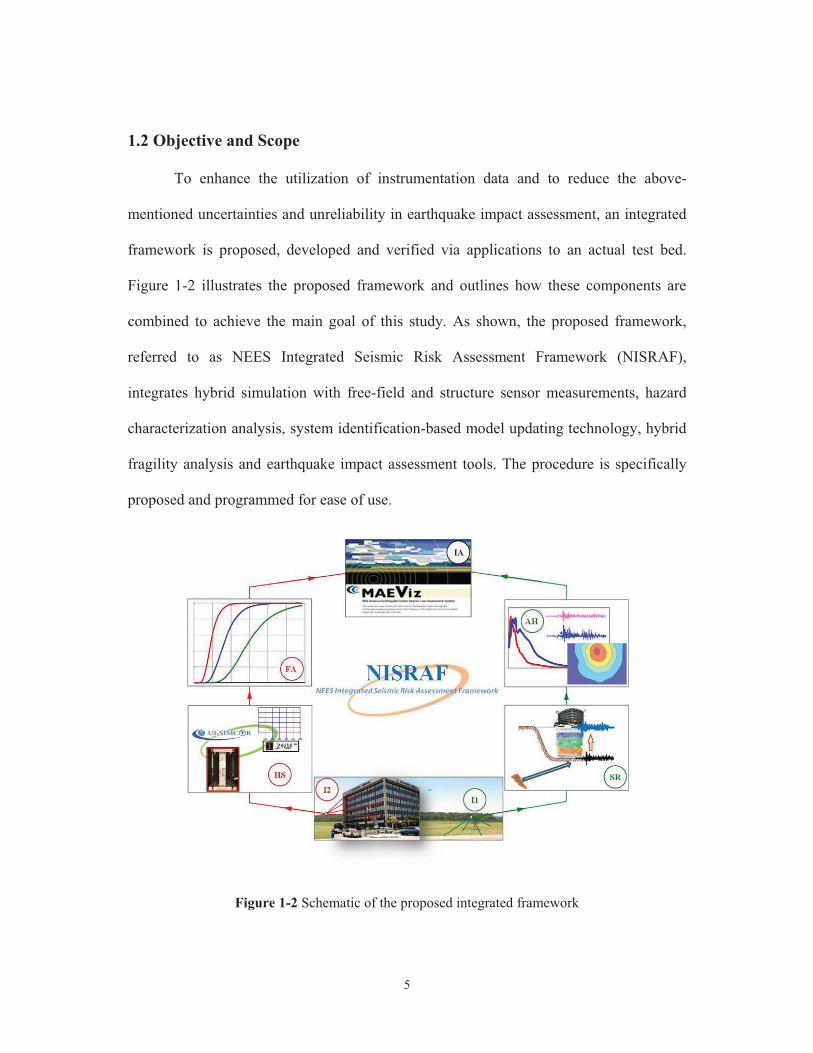
Figure 1-2 illustrates the proposed framework and outlines how these components are
combined to achieve the main goal of this study. As shown, the proposed framework,
referred to as NEES Integrated Seismic Risk Assessment Framework (NISRAF),
integrates hybrid simulation with free-field and structure sensor measurements, hazard
characterization analysis, system identification-based model updating technology, hybrid
fragility analysis and earthquake impact assessment tools. The procedure is specifically
proposed and programmed for ease of use.
Figure 1-2 Schematic of the proposed integrated framework

6
The integration feature provides an opportunity to bring together all the sub-
disciplines, capitalizing on the respective advances of each sub-discipline. This method
of integration is not only intended to provide a tool but also to stimulate the sub-
communities of researchers to investigate the problems at the interactions between them.
As part of this study, the following tasks were completed:
� Task 1: Literature review of past research and development in earthquake
engineering. Focus is given on the sub-disciplines which are needed for the
proposed framework.
� Task 2: An advanced hazard characterization method, consistent with the above
framework, which uses free-field measured data and a 1-D site response analysis
program to perform site characterization is proposed, verified and implemented in
NISRAF.
� Task 3: An advanced hybrid method for fragility derivation, suitable for
framework integration, which uses structural responses from hybrid simulation
results along with findings from the literature is proposed, verified and
implemented in NISRAF.
� Task 4: A framework—NISRAF, which combines free-field and structure sensor
measurements, system identification-based model updating techniques, hybrid
simulation, hybrid fragility analysis and earthquake impact assessment tool, is
developed and programmed for ease of use in order to obtain the most reliable
earthquake impact assessment results possible.
7
� Task 5: A pilot implementation of this framework and its components using an
instrumented structure from which high-quality measurements have been obtained
is demonstrated.
� Task 6: A pilot implementation of this framework and its components on a
modern, urbanized region is demonstrated.
1.3 Organization of Dissertation
This dissertation is conceptually composed of three main parts: namely, (i)
introduction and background information, (ii) methodology of the integrated framework
and its components, and (iii) case studies. For presentation purposes, the dissertation is
comprised of seven chapters:
� Chapter 1. Introduction: Introduces the background and objectives, and defines
the scope of this study.
� Chapter 2. Literature Review: Reviews previous research on all the components
implemented in the proposed framework. Discusses the existing methods.
Identifies drawbacks and deficiencies in current approaches.
� Chapter 3. An Advanced Hazard Characterization Analysis Method: Presents and
demonstrates the proposed advanced method for hazard analysis.
� Chapter 4. Fragility Analysis by Hybrid Simulation: Presents and demonstrates
the proposed advanced method for fragility analysis.

8
� Chapter 5. Development of NEES Integrated Seismic Risk Assessment Framework:
Presents the development of the integrated framework—NEES Integrated Seismic
Risk Assessment Framework (NISRAF). Discusses its features, potentials,
limitations and challenges.
� Chapter 6. Case Studies: Presents verifications of NISRAF via an actual test bed
in the Los Angeles area, including earthquake impact assessment, both on single
building and on an urbanized region.
� Chapter 7. Conclusions and Recommendations: Summarizes the major findings
from the development of this framework. Limitations are identified and
recommendations are made for additional research.

9
CHAPTER 2
LITERATURE REVIEW
2.1 Introduction
The components of the proposed framework are defined in Chapter 1. They
comprise free-field and structural instrumentation, seismic hazard characterization, model
calibration (including system identification and model updating), hybrid simulation,
fragility analysis and impact assessment software. Below, the main components that are
implemented in the integrated framework are reviewed.
2.2 Free-Field and Structural Instrumentation
A growing realization of the importance of the physical measurements of the
ground motions and response of structures during earthquakes, the number and coverage
of free-field and structural response instruments have increased significantly in recent
decades. Tens of thousands of free-field strong motions as well as structural instrumented
records are archived in many database centers, such as the Advanced National Seismic
System (ANSS), the Consortium of Organization for Strong Motion Observation Systems
(COSMOS), the Center for Engineering Strong Motion Data (CESMD), the PEER NGA
Database, and the California Strong Motion Instrumentation Program (CSMIP) of the

10
California Geological Survey (CGS). In the following sections, more introductions about
the developments for the above instrumentation programs and datacenters are provided.
2.2.1 ANSS, Advanced National Seismic System
Advanced National Seismic System (ANSS) is a national network under U.S.
Geological Survey established with the mission to provide real-time records and
information products for seismic events through modern monitoring methods and
technologies. Four basic goals are made for ANSS: (i) Establish and maintain an
advanced infrastructure for seismic monitoring throughout the United States. (ii)
Continuously monitor earthquakes and other seismic disturbances, for instance, the
tsunami and volcanic eruption, throughout the United States. (iii) Thoroughly measure
strong earthquake shaking at ground sites and in buildings and critical structures. (iv)
Automatically broadcast information when a significant earthquake occurs. To achieve
these goals, over 7000 sensor systems will be established in a nationwide network. The
sensors will be both on the ground and in structures (USGS, 1999).
For its monitoring activities feature, as well as making instrumentation data more
accessible, several applications based on the measured records have been proposed and
released. ShakeMap (http://earthquake.usgs.gov/earthquakes/shakemap/), with real-time
seismic intensity information shown in contour map, is generated automatically within
minutes after earthquake occurs. PAGER, Prompt Assessment of Global Earthquakes for
Response (http://earthquake.usgs.gov/earthquakes/pager/), is a program which uses

11
ANSS instrumented data along with empirical equations to provide early fatality and
economic loss following significant earthquake worldwide.
2.2.2 COSMOS, the Consortium of Organizations for Strong Motion Observation
Systems
The Consortium of Organization for Strong Motion Observation System
(COSMOS) is an international alliance aiming to maintain, communicate and archive all
the earthquake records worldwide. With the contributing members around the world,
COSMOS archives a great amount of real-time earthquake records.
Recently, Geotechnical Virtual Data Center has been established and is available
to the public for the purpose of increasing the values and use of the archived data by
incorporating the data with geotechnical information in an interactive map format.
Meanwhile, annual meeting and periodical workshops are held to discuss current
developments and applications of the instrumented data.
2.2.3 CESMD, Center for Engineering Strong Motion Data
The Center for Engineering Strong Motion Data (CESMD) is a datacenter
established by U.S. Geological Survey (USGS) and California Geological Survey (CGS).
The mission of CESMD is to integrate strong-motion data from the CGS California
Strong Motion Instrumentation Program, the USGS National Strong Motion Projects and
the ANSS. Both raw and processed strong-motion data are stored in the datacenter for
earthquake engineering applications.

12
2.2.4 Pacific Earthquake Engineering Research Center (PEER) NGA Database
The PEER NGA Database is an update and extension to the PEER Strong Motion
Database, which was published in 1999. Larger sets of records are stored in the database,
but only acceleration time history files are available currently.
For its larger set of records and more extensive data, five sets of ground-motion
attenuation models—Next Generation of Ground-Motion Attenuation Models for the
western United States (NGA West)—were developed and are available to the public
(Power et al., 2008).
2.2.5 CSMIP, California Strong Motion Instrumentation Program
The California Strong Motion Instrumentation Program (CSMIP) was established
in 1972 by California Legislation to obtain vital earthquake data for the engineering and
scientific communities through a statewide network of strong motion instruments (Naeim,
2005). More than 900 stations, including 650 ground-response stations, 170 buildings, 20
dams and 60 bridges are installed statewide. With the earthquake monitoring devices,
accelerographs, real-time records are recorded when earthquakes occur.
With heavily instrumented structures, CSMIP provides case study opportunities
for researchers to evaluate structural design procedures as well as to review the design
provisions. Performance-based seismic evaluation (Kunnath et al., 2004) and evaluation
of building period (Kwon and Kim, 2010) are two examples.
13
Indeed, with the increase of the real-time records, both quantitatively and
qualitatively, researchers and experts in many fields have benefited. For example, the
significant earthquakes provide critical information for emergency planning; the
structural engineers improve their understanding about the structural responses during
earthquakes; while the geotechnical engineers learn more about the site effect based on
specific records, and the seismologists, with the high-quality and various records, are
capable of investigating the propagation of seismic waves. However, when comparing
with the quality and quantity of instruments and captured data, the above benefits are
disproportional. That is the reason that focus is given to the applications of these valuable
data in recent years.
2.3 Seismic Hazard Characterization
Due to its stochastic nature, it is difficult to predict accurately the occurrence
(including the date and location) and the intensity of a future earthquake event. Similarly,
for its complicated and nonlinear behavior, it is also formidable to simulate realistically
the soil and topographic effects. Researchers have been devoted to the study of seismic
hazard characterization analysis to improve their understanding on seismic hazard.
Considerable understanding and significant development have been made in the past few
decades. In general, earthquake attenuation relationship, synthetic (artificial) ground
motion generation, and site response analysis contribute to current developments in
seismic hazard analysis. Below, the development of attenuation relationship is reviewed
14
with a focus given to research specifically addressing from recent comprehensive
database. Next, a review of methodology and program of synthetic ground motion
generation and site response analysis is provided.
2.3.1 Attenuation Relationship
Attenuation relationship or ground motion prediction equation (GMPE), an
empirical equation regressed from a great amount of historical earthquake records, is
used to predict the seismic intensity (in peak ground parameters or spectral ordinates).
During the past decades, several studies have been conducted which contribute the
proposal of various equations to estimate the attenuation of ground motions (Ambraseys
and Bommer, 1991; Rinaldis et al., 1998; Tong and Katayama, 1998; Takahashi et al.,
2000; Boore et al., 1997; Campbell, 1997; Youngs et al., 1997; Campbell and Bozorgnia,
2003; Ambraseys and Douglas, 2003). Recently, a set of more comprehensive attenuation
equations specifically for western United States is presented in a research project, the
Next Generation of Ground-Motion Attenuation (NGA) project (Power et al., 2008). This
project was coordinated by the Lifelines Program of PEER, in partnership with the U.S.
Geological Survey and the SCEC (South California Earthquake Center). The proposed
equations are regressed from the numerous records in the PEER NGA Database, as
described in the previous section. The objective of this project is to provide new ground
motion prediction equations through a comprehensive and highly interactive research
program. Five NGA models are presented in this project, namely, Abrahamson and Silva,
2008 (AS08); Boore and Atkinson, 2008 (BA08); Campbell and Bozorgnia, 2008 (CB08);
Chiou and Youngs, 2008 (CY08); and Idriss, 2008 (I08). A comprehensive description of
15
the Campbell and Bozorgnia NGA model (2008) is given below to explain how to
perform seismic hazard analysis using NGA models.
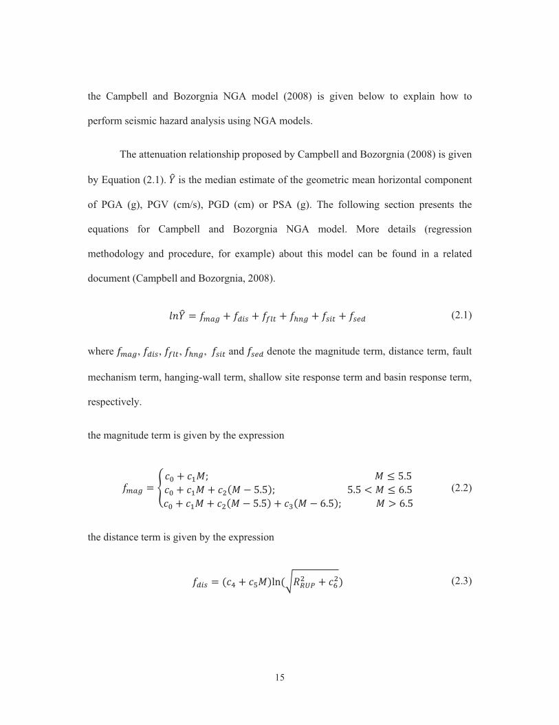
The attenuation relationship proposed by Campbell and Bozorgnia (2008) is given
by Equation (2.1). �� is the median estimate of the geometric mean horizontal component
of PGA (g), PGV (cm/s), PGD (cm) or PSA (g). The following section presents the
equations for Campbell and Bozorgnia NGA model. More details (regression
methodology and procedure, for example) about this model can be found in a related
document (Campbell and Bozorgnia, 2008).
���� � ���� � ���� � ���� � ���� � ���� � �� � (2.1)
where ����, ����, ����, ����, !���� and �� � denote the magnitude term, distance term, fault
mechanism term, hanging-wall term, shallow site response term and basin response term,
respectively.
the magnitude term is given by the expression
���� � "#$ � #%&' !!!!!!!!!! & ( ���#$ � #%& � #)*& + ���,' ��� - & ( .��#$ � #%& � #)*& + ���, � #/*& + .��,' & 0 .�� (2.2)
the distance term is given by the expression
���� � *#1 � #2&,34*56789) � #:), (2.3)

16
the fault mechanism term is given by the expressions
���� � #;<7=����>? � #@<AB (2.4)
���� � C�DE7' �DE7 - ��' �DE7 0 � (2.5)
the hanging-wall term is given by the expressions
!���� � #F����>7����>B����>?����>G (2.6)
����>7 �HIJIK �'!!!!!!!!!!! !!!!!!!!!!!!!!!!!!!!!!!!!! !!!!!!!6LM � �NOPQ R6789> 56LM) � �S + 6LMT OPQ R6789> 56LM) � �S ' 6LM 0 �> �DE7 - �U6789 + 6LM6789 '!!!!!!!!!!!!!!!!!!!!!!!!!!!!!!!!!!!!!!!!!!!!!!!!!!!!!!!!!!!!!!!!!!!!!!!!!!!!!!!!!!!!6LM 0 �> �DE7 V �
(2.7)
����>B � W�' & ( .���*& + .��,' .�� - & - .���' & V .�� (2.8)
����>? � C �' �DE7 V ��*�� + �DE7,X��' � ( �DE7 - �� (2.9)
����>G � C �' � V Y�*Z� + �,X��' � ( � - Y� (2.10)
17
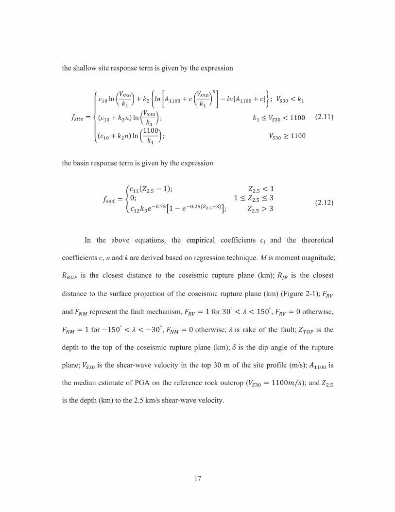
the shallow site response term is given by the expression
���� �HIIJIIK #%$ 34 R[/$ % S � ) \�� ]^%%$$ � # R[/$ % S�_ + ��`^%%$$ � #ab ' [/$ - %*#%$ � )�, 34 R[/$ % S '!!!!!!!!!!!!!!!!!!!!!!!!!!!!!!!!!!!!!!!!!!!!!!!!!!!!!!!!!! ! % ( [/$ - ����*#%$ � )�, 34 R���� % S ' !!!!!!!!!!!!!!!!!!!!!!!!!!!!!!!!!!!!!!!!!!!!!!!!!!!!!!!!!!!!!!!!!!! 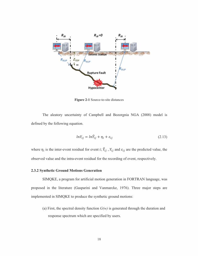
18
Figure 2-1 Source-to-site distances
The aleatory uncertainty of Campbell and Bozorgnia NGA (2008) model is
defined by the following equation.
����l � �����l � m� � n�l (2.13)
where m� is the inter-event residual for event o;!���l ,!��l and n�l are the predicted value, the
observed value and the intra-event residual for the recording of event, respectively.
2.3.2 Synthetic Ground Motions Generation
SIMQKE, a program for artificial motion generation in FORTRAN language, was
proposed in the literature (Gasparini and Vanmarcke, 1976). Three major steps are
implemented in SIMQKE to produce the synthetic ground motions:
(a) First, the spectral density function G(w) is generated through the duration and
response spectrum which are specified by users.

19
(b) Next, the peak ground acceleration (PGA) of the event and a deterministic
envelope function I(t) are defined to reflect the transient characterization of a
real earthquake.
(c) Finally, an iterative procedure is implemented in order to smoothen the
calculated spectrum and to improve the matching.
As described above, the PGA, response spectrum and duration are the only pre-
required information for SIMQKE to produce the synthetic ground motions. Owing to its
ease of use and efficiency of computation, it has been a widely used tool for ground
motion generation since its release in 1976.
2.3.3 Site Response Analysis
The significance of local site effect on ground shaking and structural response has
been known for many years. The surface ground motions may be amplified in some kinds
of soil deposits, while attenuated in others. Several clear examples can be found in recent
significant earthquakes, such as Mexico City, 1985 (Stone et al., 1987), San Francisco
Bay Area, 1989 (Seed et al., 1990) and others.
Generally, the amplitude, frequency and duration of ground shaking are critically
affected by the local site condition. The influence of site condition depends on the soil
profiles at the site as well as the topography around. In addition, the input motions are
believed to have substantial influence upon the results. Two methods are usually used to
account for site effects, namely, site-specific development and code-based development
(Kramer, 1996). The site-specific approach is based on empirical observation (Figure 2-2)

20
or analytical simulation (for example, site response analysis). Contrarily, for the code-
based development, site specific parameters are provided in the codes on account of the
different soil types, such as Fa and Fv in NEHRP recommended seismic provisions
(FEMA, 2009). The code-based approach is believed to be relatively conservative due to
the application to a broad region with the same soil parameters. In contrast, the analytical
approach has the ability to present the complicated and nonlinear behaviors in the soil.
Several analytical methods have been proposed in the past decades, varying from three-
dimensional (3-D), two-dimensional (2-D), to one-dimensional (1-D) approaches.
Generally, the 3-D and 2-D methods can provide the most realistic results. However, their
computational costs are relatively higher and the treatment of the finite element models is
also questionable. Therefore, the 1-D ground analysis method is currently the most
commonly used approach in the geotechnical earthquake engineering. SHAKE91 (Idriss
and Sun, 1992) and DEEPSOIL (Hashash et al., 2009) are the two leading site response
analysis programs which use the 1-D approach to perform local site effect analyses. In 1-
D approach, soil profiles are idealized as many layers of homogeneous soil. Then the
response of soil is calculated based on the vertical wave propagation. The continuous
solution to the wave equation can be calculated in frequency domain (SHAKE91 and
DEEPSOIL) or time domain (DEEPSOIL). Below, a review on the features of these two
programs is given.

21
Figure 2-2 Average normalized response spectra (5% damping) for different local site condition
(Kramer, 1996)
2.3.3.1 SHAKE91
SHAKE91 (Idriss and Sun, 1992), modified based on SHAKE (Schnabel et al.,
1972), is a computer program for seismic response analysis of horizontally layered soil
deposits. When performing SHAKE91, users need to define the soil properties for each
sub-layer (shear-wave velocity, shear modulus, damping and total weight, for example)
and select the input motions. In addition, the modulus reduction versus shear strain
relationship and damping ratio versus shear strain relationship must be specified to
represent the soil material properties. An equivalent linear analysis procedure is
implemented in SHAKE91 to account for nonlinear response of soil. The outputs of the
program are the time histories requested by users. In addition, many associated types of

22
data can be outputted, upon users’ request, such as the maximum shear stress and strain,
maximum acceleration, response spectrum, Fourier spectrum and amplification spectrum.
2.3.3.2 DEEPSOIL
DEEPSOIL (Hashash et al., 2009) is a 1-D site response analysis program with an
intuitive graphical user interface. Both equivalent linear and nonlinear analysis
approaches can be performed in this program. Similar to SHAKE91, the pre-requisite for
a site response analysis is the development of a soil column that is fully representative of
the study site condition. The major features in DEEPSOIL are (i) both 1-D equivalent
frequency domain and nonlinear time domain analysis approaches available, (ii) MRDF
pressure-dependent hyperbolic model, (iii) new procedures for nonlinear parameters
selection and fitting, (iv) new small-strain damping formulation, (v) the intuitive
graphical user interface, and (vi) the batch mode analysis.
Hazard stands for the demand in earthquake impact assessment. The fidelity of
hazard characterization, hence, masters the realism and reliability of the assessment
results, which underpins the emergency response and recovery planning of stakeholders.
Owing to its highly complicated and nonlinear behaviors, many obstacles and
uncertainties still need to resolve, even though substantial understanding and various
simulation methods have been made. However, the hazard characterization can be more
realistic than ever—based on the strength of the mature developments (attenuation

23
relationship, synthetic ground motion generation and site response analysis), alongside
the high-quality and various instrumentation arrays.
2.4 Model Calibration
Finite element (FE) model simulation provides a powerful way to understand the
response of buildings and other structures. However, even well constructed models may
produce significant differences in some dynamic response predictions, in particular when
the structure behaves nonlinearly. The difference results from the uncertainties of the
material properties, boundary conditions and the contributions from the non-structural
elements in the real structures. In order to resolve this drawback, system identification
based on the experimental or real instrumented response, along with model updating
techniques, is undertaken to derive the most accurate FE model. A brief review of these
two techniques is presented in the next few paragraphs.
2.4.1 System Identification
The basic concept of system identification is using the recorded sensor histories
on the structure to identify the mode shapes and frequency of the real structure. Among
the state-space based system identification methods, Eigensystem Realization Algorithm,
ERA (Juang and Pappa, 1985) is widely adopted for its good performance in multi-input
multi-output (MIMO) problems. The basic idea of ERA is to find a minimum realization
of system (state-space representation with minimum dimension) using Singular Value
Decomposition (SVD) on the Hankel matrix built by Markov parameters (impulse

24
response functions), so that the modal properties can be extracted from the realized
minimum state-space representation.
2.4.2 Model Updating
Model updating aims to minimize the discrepancy between the numerical and the
actual model by manipulating the stiffness and mass matrices. An objective function is
constructed with modal parameter (such as natural frequencies and mode shapes)
residuals which represent this discrepancy. Approaches used for model updating can
generally be sub-divided into two groups, namely, the direct method and the iterative
method. In the direct method, stiffness and mass matrices are changed directly (Minas
and Inman, 1990; Friswel and Mottershead, 1995). While for the iterative method, the
physical parameters are updated directly (Wu and Li, 2004).
To keep the sparse feature and physical meaning of the stiffness and mass
matrices, structural parameters, instead of the matrices themselves, are modified in an
iterative manner automatically through the specified optimization algorithms.
Theoretically, all parameters that are potentially inaccurate in the model and, hence, will
affect the model properties should be included in the candidates. However, a large
number of parameters may issue a huge challenge to the optimization algorithms and also
the computation capacity. Therefore, parameters for model updating should be selected
carefully based on engineering judgment and sensitivity analysis.

25
2.5 Dynamic Response Simulation of Structures
Being aware of the vital role of structural response to assessment and mitigation
of earthquake loss, advanced simulation techniques have been developed in order to
duplicate the real structural behaviors. With the improved knowledge and development in
both structural engineering and computation, an evolution has been presented from
analytical finite element model simulation to laboratory testing, such as Pseudo-Dynamic
Test (PSD) and shaking table testing. Recently, an advanced simulation technique—
hybrid simulation—has been proposed and showcased potentials via its coordination and
geographically distributed features. Below, a review of the simulation techniques in the
order of evolution is given.
2.5.1 Model Analytical Simulation
Analytical model, which is developed based on the principles of mechanics and/or
calibrated with the experimental data, provides an alternative way to predict the response
of structures efficiently. Several finite element (FE) model simulation programs have
been developed and released in the past decades, such as ZEUS-NL (Elnashai et al.,
2004), OpenSees (McKenna and Fenves, 2001), ABAQUS (Hibbit et al., 2001), Vector2
(Vecchio and Wong, 2003), PISA3D (Lin et al., 2006) and others. ZEUS-NL, a product
of Mid-America Earthquake Center has plate, shell and solid elements. OpenSees,
developed by the Pacific Earthquake Engineering Research Center, focuses on the
geotechnical constitutive models. ABAQUS, a commercial program, has extensive
element libraries, but limited capabilities in conducting reinforced concrete analysis.

26
In addition to analytical simulation, laboratory (or experimental) simulation
provides an alternative to understand structural behaviors. Static, dynamic and shake
table testing are the most commonly used simulation techniques for experimental
simulations. Among them, shake table testing with a full scale structure can provide the
most realistic response. However, most of the tables are small, and their capacities are
limited. Moreover, the cost of testing is relatively high. Many alternative methods have
been developed and evolved during the past decades with different research purposes as
well as the development of computation techniques.
2.5.2 PSD, Pseudo-Dynamic Test
Pseudo-Dynamic Test (PSD) was developed to alternate the real-time shake table
testing. In PSD, the inertial and damping force are calculated in the analytical models,
and, after that, the corresponding displacements are applied to the structures. The concept
of PSD was first proposed by Takanashi in Japan (Takanashi et al., 1975). Since that,
several PSD tests have been performed around the world (Mahin and Shing, 1985;
Nakashima et al., 1987; Elnashai et al., 1990; Jeong and Elnashai, 2004; Chen et al.,
2003).
2.5.3 Hybrid Simulation
Pseudo-Dynamic Test is applicable to large-scale tests in the laboratory. However,
PSD may suffer problems due to the limitation of the facility capacity in the laboratory.
Meanwhile, as described previously, each FE program has its own strengths and
weaknesses. In order to capitalize the strengths of each module (FE program or

27
laboratory facility), UI-SIMCOR—a hybrid simulation software platform—was proposed
and developed (Kwon et al., 2007). Although UI-SIMCOR uses the same integration
scheme as that in PSD, its geographically distributed feature allows unlimited modules
(analytical or experimental, domestic or international) to be combined within the
simulation. Currently, the modules can be experimental specimen or analytical models in
OpenSees (McKenna and Fenves, 2001), ZEUS-NL (Elnashai et al., 2004), ABAQUS
(Hibbit et al., 2001), FedeasLab (Filippou and Constantinides, 2004) and Vector2
(Vecchio and Wong, 2003). Hybrid simulation—defined as the combination of physical
(or experimental) testing and analytical models—is used here to be distinguished from
multiplatform simulation, in which all the sub-structures are simulated analytically.
Several multiplatform and hybrid simulation tests (including small and large scale) have
been conducted and approved its coordination and communication features (Spencer et al.,
2006; Spencer et al., 2007).
Analytical and experimental simulation provides a way to understand seismic
behavior of structures. Hybrid simulation, indeed, promotes the ability to evaluate
structural behaviors never before available. However, at its younger age, more
verification about its components as well as the interaction between other sub-disciplines
is essential for its integrity and robustness.

28
2.6 Fragility Analysis
Fragility, or vulnerability is defined as the conditional probability that a structure
or a structural component would reach or exceed a certain damage level for a given
ground motion intensity. Through the application of fragility curves, loss from
earthquake hazard can be easily estimated. Mathematically, a fragility relationship can be
defined as:
p� � p N�q V �T (2.14)
where p� is the failure probability for a specific damage state; � is the structural demand,
and q is the structural capacity. In Equation (2.14), structural demand � depends on
earthquake ground motion intensity.
Significant contribution has been made in the field of fragility analysis in the past
few decades. A comprehensive review on the development of fragility assessment,
specifically addressing methodologies over the past 30 years was presented in the
literature (Calvi et al., 2006). Generally, fragility curves can be sub-divided into four
categories based on data sources, namely, empirical fragility curves, judgmental fragility
curves, hybrid fragility curves and analytical fragility curves (Rossetto and Elnashai,
2003).
Empirical fragility curves are developed through field investigations after
earthquakes—are the most realistic. However, this observation data is scarce and
clustered in the low damaged range. Judgmental fragility curves are based on expert
opinion, and are therefore subjective. Unlike the empirical and judgmental fragility
curves, analytical fragility curves are more general. Curves can be generated for different
29
limit states and different structural types, although at a higher computation cost.
Meanwhile, the selection of the models and the simulation methods will significantly
affect the accuracy of the curves. Due to the above limitations, most analytical fragility
curves are generated either by simple models or by complicated models without
calibration to measured response, which can result in uncertainties in these curves.
Hybrid fragility curves are proposed to compensate the scarcity, subjectivity and
modeling deficiency in experimental, judgmental and analytical fragility curves,
respectively. Two approaches are generally used to derive hybrid fragility curves, namely,
fragility relationships calibrated with other source and fragility relationships combined
with others. In the first one, empirical data is generally used to calibrate the judgmental
or analytical fragility curves. While in the other one, two different types of fragility
curves are combined to derive fragility relationships, such as analytical curves along with
empirical curves from historical earthquakes. Presumably, hybrid fragility curves
capitalize advantages from different types of fragility curves. Limitations and challenges,
however, still remain for the reasons that each type of fragility has its own uncertainties,
and the analytical fragility relationships cannot be really improved by only a small
portion and maybe clustered of empirical data.
2.7 Earthquake Impact Assessment Tools
Earthquake impact assessment tools have been already extensively adopted by the
stakeholders in the community for risk management. The realism of the outcomes, such
as the effect on the infrastructure systems, economy and societal activities are the

30
essential ingredients of the emergency response and recovery planning—which will then
adequately protect our vulnerable communities.
In recent years, significant progress has been made in earthquake impact
assessment, including consequence estimation methodology as well as developing
software that provides decision-makers with a tool to assess the impact. Currently, many
software tools using different methodology able to estimate seismic losses have been
developed and released. Among the leading software tools are HAZUS-MH (FEMA,
http://www.fema.gov/plan/prevent /hazus/), MAEviz (Mid-America Earthquake Center,
http://mae.ce.uiuc.edu/software_and_tools/maeviz. html), RMS (Risk Management
Solutions, http://www.rms.com/catastrophe/software/), AIR (AIR Worldwide
Corporation, http://www.air-worldwide.com/_public/html/modeltech.asp), KOERILOSS
(Bogazici University, http://fatin.koeri.boun.edu.tr/depremmuh/EXEC_ENG.pdf), and
others. In the following review, a focus is placed on HAZUS-MH (FEMA, 2006) and
MAEviz (MAE Center, 2007). The reason underlining this selection is that HAZUS-MH
is a public package supported by FEMA, the federal agency responsible for disaster
response planning, and MAEviz is the open-source platform of the MAE Center, where
new models and linkages can be easily implemented. Moreover, as discussed in Chapter
1, the reliability of assessment results is very much dependent on the hazard
characterization and fragility curves. Therefore, focus is given to methodology of hazard
and fragility components.

31
2.7.1 MAEviz
MAEviz, an earthquake consequences assessment package, which follows the
Consequence-based Risk Management (CRM) paradigm, has been developed by the
MAE Center and the National Center for Supercomputing Applications (NCSA) at the
University of Illinois (MAE Center, 2007). CRM is a new paradigm for seismic risk
reduction across regions or systems that incorporates identification of uncertainty in all
components of seismic risk modeling and quantifies the risk to societal systems and
subsystems.
MAEviz provides more than 40 types of analysis models from building, bridge,
utility and transportation networks, socioeconomic, to decision support analysis. With
these various analyses and its interactive-visual feature, MAEviz provides the
stakeholders with assessment information for developing plans and mitigation for future
seismic events.
Deterministic hazard approach is implemented in MAEviz. Therefore, users are
prompted to define seismic parameters and select attenuation equations to generate the
seismic hazard. Moreover, the code-based method, i.e. Fa and Fv site specific coefficients
in NEHRP provisions (FEMA, 2009) is adopted to account for local site effects. Due to
the probabilistic nature and approximate method, uncertainties remain in the procedure
and outcome. For the fragility component, numerous fragility models developed by
researchers for different types of structures are archived in MAEviz database. A mapping
file is therefore required to match the fragility curves with different types of structures.
32
Among these archived fragility relationships, however, most of them are from simple
models (Single Degree of Freedom, SDOF) or complicated models without calibration to
the real response of a physical structure. Such methods, therefore, introduces significant
and by-and-large uncertainties in the derived fragility curves.
2.7.2 HAZUS-MH
HAZUS-MH, a risk assessment package, is developed by Federal Emergency
Management Agency to estimate the potential losses from floods, hurricane winds and
earthquakes (FEMA, 2006). The HAZUS-MH earthquake model can provide the
estimation of damage and loss to buildings or lifelines under the scenario earthquakes, for
example, the damage to the buildings, the direct or indirect cost during events, and
displacement of households or the requirement of shelters.
Both deterministic and probabilistic hazard approaches are implemented in
HAZUS-MH. For the deterministic method, similar to the procedures in MAEviz, user
needs to define the seismic parameters and select attenuation equations. While in the
probabilistic method, the hazard maps generated by USGS are implemented in HAZUS-
MH, which allows users to select a map specific to different hazard levels for analysis.
The code-based method—multiplying by Fa and Fv parameters, same as MAEviz—is
adopted in both deterministic and probabilistic approaches.
Unlike the straightforward methodology in MAEviz, capacity spectrum method
(CSM) is implemented in HAZUS-MH to calculate the degree of damage of structures as
well as the related societal activities. Briefly, the structural capacity and fragility

33
relationships in HAZUS-MH are defined based on expert opinions and judgments. The
assumed bilinear capacity curve and the hazard demand curve, along with CSM, are used
to derive the structural response. Structural nonlinear behavior is reflected only by simply
scaling the demand curve. Although its efficiency, this simplified approach does not
explicitly consider the influence of structural parameters, such as damping, period and
yield strength level.
2.8 Summary and Discussion
The components required for this proposed framework are in a sufficiently mature
state. The increase in network density and applications reinforces the role of strong-
motion instruments in the seismic community. Ground motion prediction equations,
synthetic ground motions and site response analysis are all in their mature states, which
allow to present hazard characterization probabilistically. The potential of hybrid
simulation has been shown previously. Fragility analysis and model calibration
techniques both have their substantial development. Impact assessment also has reached
its mature state and has been extensively used worldwide.
Nevertheless, uncertainties, simplification and engineering judgment still remain
in the procedures and outcomes, as discussed previously. An integrated, transparent and
systematic framework, therefore, provides an opportunity to reduce and manage the
uncertainties and assumptions. Through the proposed integrated framework—NEES
Integrated Seismic Risk Assessment Framework, NISRAF—uncertainties from each sub-

34
discipline can be managed more effectively and the utilization of the instrumentation will
increase. For example, the reliability of probabilistic seismic hazard can be significantly
improved through the use of free-field strong-motion measurements. Analytical and
hybrid (analytical-experimental) simulations can be realistic due to calibration with
system identification results from sensor measurement. The uncertainties from deriving
fragility relationships can be greatly reduced through the use of more reliable
representation of hazard and more accurate structural models. Confidently, with seismic
hazard from field measurements and fragility curves derived from accurate models,
NISRAF can significantly improve upon earthquake impact assessment results.
To achieve a seamless integration and to arrive at an operational and verified
system, the above components are used innovatively, tailored to perform the role required
by NISRAF. The integrated system brings the most advanced tools of earthquake hazard
and structural reliability analyses into the context of societal requirement for accurate
evaluation of the impact of earthquakes on the built environment.
In the following sections of this dissertation, an advanced hazard characterization
method and an advanced hybrid fragility analysis method are proposed and demonstrated
first. Development of the proposed framework, which integrates components from sensor
data to seismic loss assessment, is then presented, followed by verifications and case
studies.

35
CHAPTER 3
AN ADVANCED HAZARD CHARACTERIZATION
ANALYSIS METHOD
3.1 Introduction
Several countries around the world have to face threatening earthquakes and
related hazards, such as tsunami. Historical earthquakes have revealed their power to
devastate structures, to cause fatalities and to disrupt human society (Figure 1-1). Owing
to the uncertainties from seismo-tectonic, earthquake energy attenuation and site
conditions, it is difficult to estimate accurately the ground motion parameters. Many
methods for seismic hazard analysis have been developed over the past decades. Among
them, Deterministic Seismic Hazard Analysis, DSHA (Reiter, 1990) and Probabilistic
Seismic Hazard Analysis, PSHA (Cornell, 1968) are the most commonly used methods,
and both are generally implemented within the earthquake impact assessment packages,
such as MAEviz (MAE Center, 2007) and HAZUS-MH(FEMA, 2006). Due to the
probabilistic nature and the simplified assumption for the local site effect, such as the use
of the site coefficients Fa and Fv, uncertainties remain in the procedure and outcome. To
reduce these uncertainties, an advanced hazard characterization analysis method is
proposed—which uses free-field measured data and 1-D site response analysis program
to perform site characterization.

36
3.2 Overview of the Advanced Hazard Characterization Analysis Method
The advanced hazard approach is mainly composed of four parts: (a) seismic
hazard analysis, (b) synthetic ground motion generation, (c) site response analysis and (d)
hazard map generation. First of all, the natural records are investigated directly to
evaluate the hazard characterization. Synthetic records—with site specific characteristics
and different hazard levels—are then generated to present the hazard as well as to provide
various ground motions for further use in hybrid simulation and fragility curve derivation.
Figure 3-1 shows the methodology and procedures of the advanced hazard
characterization analysis approach. The following sections detail the methodology and
procedures. Rather, verifications are given via an actual test bed application in the Los
Angeles area.
Figure 3-1 Methodology and procedures of hazard characterization analysis

37
3.3 Seismic Hazard Analysis
Seismic Hazard Analysis is the first step in hazard characterization analysis. In
this step, the natural records around the site of interest are investigated comprehensively.
Peak ground acceleration (PGA) and response spectra are generated and compared.
Furthermore, several tools—such as attenuation model, duration prediction and
deaggregation, which are commonly used to evaluate seismic characterization
probabilistically —are also included in this step. Seismic information is indispensable for
synthetic ground motion generation, particularly in a region where earthquake records are
absent or in lower quality. Consequently, seismic hazard characteristics—based on the
measured free-field records or deriving from probabilistic tools—are the ingredients in
the further synthetic ground motion generation, site response analysis and hazard map
generation.
3.3.1 Seismic Hazard Analysis from Natural Records
Generally, strong motion records are subdivided into three different types, namely,
(i) Measured structures with instruments on the ground, (ii) Free-field station records on
the outcrop, and (iii) Free-field station records on the surface of soil. Different analysis
procedures are conducted for different type of records.
(I) Measured structures with instruments on the ground
If the structure instrumented and has sensors installed on the ground (Figure 3-2), the
records on the ground level are utilized directly. Seismic parameters (peak ground
acceleration (PGA) and response spectra, for example) are calculated and generated
38
to present the seismic characterization at this site. Meanwhile, the natural records are
ready to be used in hybrid simulation and fragility analysis later.
Figure 3-2 Measured structures with instruments on the ground
(II) Free-field station records on an outcrop
Site response analysis is performed on outcrop free-field strong motion records
(Figure 3-3), in order to capture the local site effect. DEEPSOIL (Hashash et al.,
2009), a 1-D site response analysis program, is used to conduct the site response
analysis. As mentioned previously, a representative soil column is the prerequisite for
site response analysis. Therefore, user is prompted to define the soil profiles
(thickness, shear-wave velocity and unit weight, for example) and the material
properties (such as shear modulus reduction versus strain and damping versus strain
curves) for different soils. Surface motions with specific site characteristics are then
generated and ready for further use later.

39
Figure 3-3 Free-field records on an outcrop
(III) Free-field station records on soil surface
When records are on soil deposits surface (point A in Figure 3-4) or within soil
deposits, it is more complicated to evaluate site characterization. For record on the
surface or within soil deposits, it is first deconvolved through the soil profiles to
determine the motion on the bedrock (point B in Figure 3-4). Bedrock motion is then
propagated to the bedrock beneath the interested site (point C in Figure 3-4). Finally,
the record on the bedrock is convoluted through soil profiles to the surface (point D in
Figure 3-4).
Figure 3-4 Free-field station record on soil surface

40
Although the deconvolution concept is rational, the technology to deconvolve
ground motion through soil is still a challenge and studies are still going. Therefore, the
deconvolution procedure is not implemented in the current proposed advanced hazard
method, but will be when this technology is ready.
3.3.2 Seismic Hazard Analysis for Scenario Earthquakes
Due to the limited number and narrow intensity distribution of the natural ground
motion records, several tools have been developed and are available to derive seismic
hazard characteristics for a scenario earthquake. In this study, the latest and the most
mature research findings are integrated in a novel manner in order to provide the realistic
hazard characteristics as well as reasonable and various synthetic ground motions. NGA
attenuation models (Power et al., 2008) and duration prediction equation (Kempton and
Stewart, 2006)—both empirical equations regressed from the PEER NGA Database—are
used to derive PGA, response spectrum and duration, which are the critical ingredients in
seismic hazard analysis. With the above seismic information, SIMQKE (Gasparini and
Vanmarcke, 1976)—a widely used synthetic ground motion generation program—is
conducted to generate numerous artificial motions. Furthermore, ground motions varying
with different hazard levels are essential to capture structural responses in different
performance limit states, which in their own right are needed for fragility derivation. For
this variation requirement, deaggregation results—which provide earthquake shaking
information for different hazard levels—are therefore included in this advanced hazard
method.

41
The NGA attenuation has already been discussed in section 2.3: Seismic Hazard
Characterization. In the below section, duration proposed by Kempton and Stewart (2006)
is detailed, followed by discussion on the deaggregation technology. Rather, SIMQKE is
discussed in section 3.4 Synthetic Ground Motion Generation.
3.3.2.1 Significant duration prediction equation
Duration, the time for energy release during the ground shaking, varies with the
magnitude, distance and also the site condition. Several definitions of ground motion
duration have been proposed, such as bracketed duration (Kawashima and Aizawa, 1989),
uniform duration (Vanmarcke and Lai, 1980) and significant duration (Trifunac and
Brady, 1975). A more comprehensive review on duration of earthquake ground motions
can be referred to Bommer and Martinez-Pereira (1999).
To predict the duration, Chang and Krinitszky (1977) first proposed an empirical
relationship for duration estimation (bracketed duration with 0.05g threshold
acceleration). In the proposed prediction relationship, the duration varies with magnitude
under different site condition; i.e. rock and soil site (Figure 3-5). Recently, an equation
for significant-duration prediction has been proposed by Kempton and Stewart (2006).
This new prediction equation is derived based on the PEER NGA Database through a
random-effects regression procedure. This proposed significant-duration prediction
equation is given by:

42
34!*r,�l � 34 stuvw!*xyzxf*B{dB|,,%$y�g}{~y���g ���Z � ��:� � ��l#) � *#1 � #2*[/$,�l,� � m� � n�l (3.1)
where r is the significant duration; &| is the reference magnitude taken as 6; � is the
shear-wave velocity at the source (taken as 3.2 km/s); &� is the magnitude of event o; ��lis the distance for recording � in event!o; m� is the event term for earthquake event!o; n�l is
the residual for recording � in event o; and �� and #� are regression coefficients.
Figure 3-5 Variation of bracketed duration (0.05g threshold) with magnitude and epicentral
distance: (a) rock sites; (b) soil sites. (Kramer, 1996)
This significant-duration prediction equation proposed by Kempton and Stewart
(2006) is incorporated into the proposed advanced hazard method, not only for its

43
inherent nature (regressed from a modern database), but also for its ease for
implementation (a mathematical equation rather than a plot relationship). Moreover, to
account for the uncertainties in duration, in addition to the uncertainty term in Kempton
and Stewart’s equation, various lengths of duration—the original predicted duration and -
5%, +5%, +10%, +20% of the predicted duration—are implemented in the proposed
procedure.
3.3.2.2 Deaggregation results from Probabilistic Seismic Hazard Analysis
The probabilistic seismic hazard analysis method provides the annual rate of
exceedance at a particular site, which is from the aggregation of the potential earthquakes
of different magnitudes and different source-site distances (Kramer, 1996). However, the
information about the likely earthquake magnitude and the most likely source-site
distance is sometimes more useful for structural designers and decision makers.
Deaggregation, a resolution of the above concern, is capable of identifying scenario
events. Generally, a set of deaggregation results is composed of three components,
namely, (i) magnitude, (ii) distance and (iii) epsilon.
Magnitude (&)
The magnitude term in deaggregation result is referred to the moment magnitude.
Distance (6)
The distance term in deaggregation result means the source to site distance.

44
Epsilon (n)
The definition of epsilon is the number of standard deviations by which a given
��� value differs from the mean ��� value, based on the given magnitude and distance.
Epsilon can be presented as:
n � ��� + ���[�*&> 6,���[� (3.2)
where ���[�*&> 6, and ���[� are the predicted mean and standard deviation of !��� ,
respectively. ��� is the natural logarithm of the spectral acceleration of interest. The
first two parameters can be calculated through attenuation equations.
In addition to magnitude, distance and epsilon, information about the contributed
fault mechanism is also provided in the deaggregation results. The fault information is
also important when performing attenuation models.
3.4 Synthetic Ground Motion Generation
As a feature to provide site specific synthetic ground motions, SIMQKE
(Gasparini and Vanmarcke, 1976)—a widely used program for artificial ground motion
generation—is incorporated in the proposed hazard method. Step-by-step procedure to
generate synthetic ground motion is given below:
Step 1: At the beginning of the analysis, the user is prompted to define the seismic
parameters (magnitude, distance, fault mechanism and site condition).

45
Step 2: Spectra, specified by the user or based on ground motion prediction
equations, such as the Next Generation Attenuation (NGA) models, and
predicted duration are produced.
Step 3: Finally, synthetic ground motions are generated automatically and
efficiently through SIMQKE based on the information defined previously.
Subsequently, both the natural and synthetic records are ready to be modified to
reflect the local site condition. DEEPSOIL (Hashash et al., 2009)—a 1-D site response
analysis program—is implemented to perform the site response analysis. Site response
analysis will be fully illustrated in section 3.5 Site Response Analysis.
As illustrated in section: 2.3 Seismic Hazard Characterization, in addition to the
PGA, response spectrum and duration, an intensity function is needed to define in
SIMQKE (Gasparini and Vanmarcke, 1976). Moreover, two additional duration
parameters (Tb and Ttotal) are prompted to be defined in the proposed method. Through
the definition of intensity function as well as duration parameters, a more realistic and
reasonable ground motion is produced. Below, introduction on intensity function and the
proposed duration parameters are shown.
3.4.1 Intensity Function
To reflect the transient character of real earthquake records, a deterministic
envelope function (intensity function) I(t) needs to be defined. Two different intensity
functions are implemented—the trapezoidal and exponential functions (Figure 3-6). The
user is prompted to select one of them and define the related coefficients.

46
(a) Trapezoidal (b) Exponential
Figure 3-6 Intensity functions implemented in SIMQKE (Gasparini and Vanmarcke, 1976)
3.4.2 Duration Parameters
In SIMQKE (Gasparini and Vanmarcke, 1976), the defined duration is the period of
the major vibration of the records (as the ‘Duration’ range shown in Figure 3-7). In order
to simulate the quiet zone or small vibrations in the beginning and end of an earthquake
record, Tb and Ttotal are introduced in the proposed method, as shown in Figure 3-7.
Figure 3-7 Definition of Tb and Ttotal
DUR
I t( )
t
1.0
TRISE TLVL
TLEVEL
DUR
t tI t A e e0( ) ( )� �� �� �I t( )
t
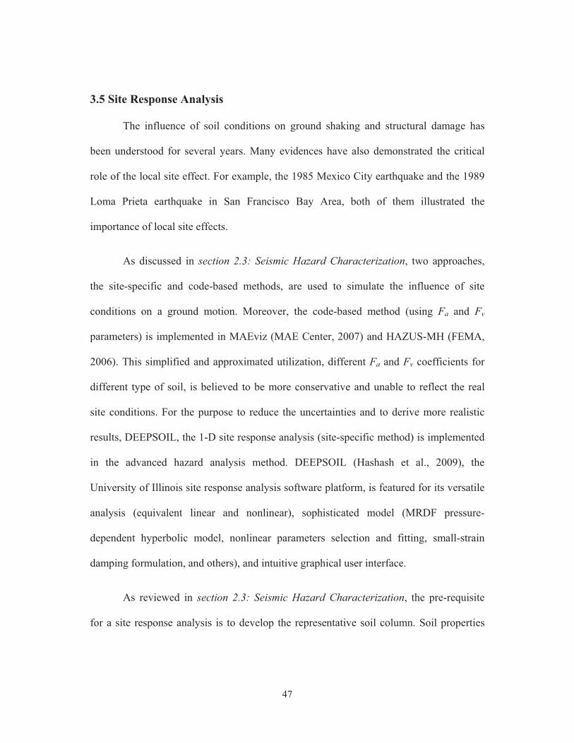
47
3.5 Site Response Analysis
The influence of soil conditions on ground shaking and structural damage has
been understood for several years. Many evidences have also demonstrated the critical
role of the local site effect. For example, the 1985 Mexico City earthquake and the 1989
Loma Prieta earthquake in San Francisco Bay Area, both of them illustrated the
importance of local site effects.
As discussed in section 2.3: Seismic Hazard Characterization, two approaches,
the site-specific and code-based methods, are used to simulate the influence of site
conditions on a ground motion. Moreover, the code-based method (using Fa and Fv
parameters) is implemented in MAEviz (MAE Center, 2007) and HAZUS-MH (FEMA,
2006). This simplified and approximated utilization, different Fa and Fv coefficients for
different type of soil, is believed to be more conservative and unable to reflect the real
site conditions. For the purpose to reduce the uncertainties and to derive more realistic
results, DEEPSOIL, the 1-D site response analysis (site-specific method) is implemented
in the advanced hazard analysis method. DEEPSOIL (Hashash et al., 2009), the
University of Illinois site response analysis software platform, is featured for its versatile
analysis (equivalent linear and nonlinear), sophisticated model (MRDF pressure-
dependent hyperbolic model, nonlinear parameters selection and fitting, small-strain
damping formulation, and others), and intuitive graphical user interface.
As reviewed in section 2.3: Seismic Hazard Characterization, the pre-requisite
for a site response analysis is to develop the representative soil column. Soil properties

48
are defined either from field reports (such as borehole logs) or based on field or
laboratory tests (Standard Penetration Test (SPT), for example).
3.6 Hazard Map Generation
Hazard Map—which contains earthquake intensity either with peak ground
parameters (PGA, PGV or PGD) or spectral ordinates (Sa, Sv or Sd)—is used to present
the hazard at a specific site. Hazard map is essential and widely used in many sub-
disciplines. For example, structural engineers use it for seismic design; insurance
companies use it to evaluate risk and develop policy. Moreover, it is an essential
component of earthquake impact assessment.
Through the tools discussed in previous sections, a hazard map is generated with
accuracy in an efficient way. Step-by-step procedure to generate hazard map is given
below:
Step 1: At the beginning of the analysis, the user is prompted to define the seismic
parameters (epicenter location, magnitude, distance, fault mechanism and
site condition, for example) for a scenario event. In addition, map
information, such as the cell size of raster data, the location (the latitude
and the longitude) of area of interest, are also needed to be specified.
Raster data here is a file contained hazard values with location information,
which is a commonly used format in Geographic Information System (GIS).

49
Step 2: PGA, response spectrum and duration are derived by the models specified
by the user. Next, these information for each cell are fed into SIMQKE
along with site response analysis to derive surface ground motions.
Step 3: Hazard Map is finally generated by collecting seismic parameters at each
cell with organization. A visual map and a raster data format file are
generated simultaneously. Raster data format file here is compatible with
MAEviz to perform earthquake impact assessment.
3.7 Verification Studies
As illustrated in previous sections of current chapter, the latest and widely used
approaches are utilized in the proposed advanced hazard characterization method. To
achieve seamlessness, to conduct the analysis efficiently and to make ease of use, the
above tools or methods are integrated in a novel manner and are tailored for user’s ease.
For example, users are only needed to define the seismic parameters in the beginning step.
Synthetic ground motions and hazard map are then generated with site response analysis
automatically. More discussion and features of this advanced hazard method is addressed
in Chapter 6 Development of NEES Integrated Seismic Risk Assessment Framework. In
the following parts of this section, several verifications are presented in order to evaluate
the achievements of this proposed advanced hazard method.
3.7.1 Introduction
The Burbank Fire Station site at Burbank, California (latitude = 34.181°,
longitude = -118.304°)—where the borehole log, and records from free-field stations and

50
instrumented buildings around are available—was selected to demonstrate the procedures
and evaluate the outcomes under the proposed hazard characterization approach.
Based on the SMIP geotechnical report No. 131 (Fumal et al., 1979), the soil
deposits at the Burbank site is Pleistocene alluvium. The borehole log (Figure 3-8) shows
the soil profile for the top 30 meters at this site. Fine Sandy Loam, Gravelly Sand and
Sandy Loam/Loamy Sand are the three soils in the top 30 meters. SPT results range from
10 blows/ft in fine sandy loam to 40 blows/6 inches in Gravelly Sand. The average
measured shear-wave velocity is 405 m/s in Fine Sandy Loam, and is 452 m/s in Gravelly
Sand and Sandy Loam/Loamy Sand (Table 3-1). The water table is assumed 20 feet
below the ground surface, based on the geologic criteria for Burbank with soil deposits of
similar Pleistocene age (Department of Conservation, Division of Mines and Geology,
1998).
Table 3-1 Soil properties of Burbank site (Fumal et al., 1979)
Depth Soil Type
SPT Density Shear-wave Velocity
(m) (Blow/ft) (gm/cc) (m/s) (avg.)
-12.5 Fine Sandy Loam 10 2.16 405
-18 Gravelly Sand 40/6” 2.16 452
-30 Sandy Loam/Loamy Sand --- 2.16 452

51
Figure 3-8 Borehole log of the Burbank site (adapted from Fumal et al., 1979)
ALTITUDE:���610'
DATE:�����8/1/79
COMMENTS: LOGGED�BY:� ���T.�FumalFigure�22
LOCATION:��������Lat.��������34°10'50"��������Long.����118°18'15"QUADRANGLE:
Blow
s/Foot
Depth
SAMPLE�DESCRIPTION
Density
(gm/cc)
Graphic
Log
MAO�UNIT:� �Pleistocene�alluvium
Sampling
(meters)
DESCRIPTION
���������BURBANK,�CA
HOLE�No.� ���31SITE:� �BURBANK�FIRE�STATION
GEOLOGIC ���Qc
FINE�SANDY�LOAM,�dk.�Brown,�some�v.coarse�sand�and�fine�gravel,�mediumplasticity,�moist,�loose.
15
10
5
0
2.16
GRAVELLY�SAND,�granitic.
30
SANDY�LOAM�and�LOAMY�SAND,�dk.Brown,�poorly�sorted,�slight�plasticity,quick,�moist,�occasional�fine�gravel�to5mm.
P20
25
FINE�SANDY�LOAM,�dk,�bBrown,occasional�v.�coarse�sand�andgravel,�medium�plasticity,�moist,loose.
SANDY�LOAM,�brown,�poorlysorted,�mostly�finer�than�coarsesand,�some�granitic�gravel,�v.dense.
SANDY�LOAM�and�LOAMY�SAND,dk.�Brown,�poorly�sorted,�slightplasticity,�quick,�moist,�occasionalfine�gravel�to�5�mm.
39
10
40/6"

52
3.7.2 Hazard Models Calibrated with Measured Records
As shown in Figure 3-9, numerous free-field stations (circle) and instrumented
buildings (square) are around the study site (Burbank, California). Meanwhile, a great
number of records are available for past earthquakes, including the Northridge earthquake
on January 17th, 1994. The hazard model may therefore be more realistic by calibration
with the measured free-field records. In the following sub-sections, comparisons are
undertaken between seismic parameters from the measured records during the Northridge
earthquake and those derived from Campbell and Bozorgnia NGA model (Campbell and
Bozorgnia, 2008)—using the Northridge earthquake mechanism along with site
information from the SMIP geotechnical report.
Figure 3-9 Free-field and structural instruments around the Burbank site (CESMD)

53
Nineteen borehole logs are available in the SMIP report. Eight of them were
selected to calibrate the Campbell and Bozorgnia NGA model, CB-NGA (2008) for the
reason that there is at least one instrument station (CSMIP station) which is close to the
borehole site (less than 5 kilometers). Records during the 1994 Northridge earthquake in
the instrument stations were used for this calibration. Consequently, site conditions from
the borehole logs and seismic mechanism of the Northridge earthquake (Table 3-2,
Figure 3-10) were used to tune the CB-NGA model. �)�2 � � �> *�� � � �, was
assumed for the absence of this information in SMIP report. Table 3-3 lists the
parameters of the borehole sites required for the CB-NGA model.
Table 3-2 Seismic parameters of the 1994 Northridge earthquake (USGS, 1996)
Magnitude (Mw) Dip (degree) Rake (degree) �DE9(km) Fault Mechanism
6.7 40 104 5 Reverse
Figure 3-10 Portrayed buried fault plane of the Northridge earthquake (USGS, 1996)

54
Table 3-3 Parameters from SMIP report required for the CB-NGA model
Borehole ID 6LM(km) 6789(km) [/$(m/s) �)�2(km)*
#31 18.7 22.0 430.1 2
#32 84.9 87.0 324.8 2
#34 53.3 56.6 407.3 2
#36 48.8 52.3 221.1 2
#38 63.1 65.9 275.1 2
#41 6.0 7.8 790.6 2
#42 5.1 7.2 453.3 2
#44 5.1 7.2 531.0 2
* No information about �)�2 from SMIP report, �)�2 � � �> *�� � � �, was assumed.
To calibrate the NGA model, two approaches are considered, namely, calibrating
the regression coefficient #� or checking the sensitivity of seismic parameters (for
example, [/$ , �)�2 and others). Due to the limited stations and records, the second
approach was conducted in this study. Sensitivity analyses of [/$ and �)�2 were
performed, for the absence of �)�2 and the use of average [/$ values. Figure 3-11 shows
a comparison using different [/$ and �)�2. The difference was defined as the square root
of sum of squares (SRSS) of the discrepancy between the measured value and the
predicted median value (CB-NGA, Campbell and Bozorgnia, 2008) at each station.
Clearly, the result was significantly affected by the �)�2 value rather than [/$. To reduce
the uncertainties, more investigation was conducted. Table 3-4 lists �%�$, �%�2 and �)�2information of the 8 selected stations. This information is from stations in the PEER
NGA Database, which are close to the 8 selected CSMIP stations (within 5 kilometers).
For sites where only �%�2 is available (for example, #42 and #44), the Equation (3.3) was

55
used to predict �)�2 (Campbell and Bozorgnia, 2007). If �%�$, �%�2 and �)�2 are unavailable,
�)�2 � � �> *�� � � �, was assumed. Table 3-5 lists the final values of �)�2.
�)�2 � ��.�. � ����Z�%�2 (3.3)
Figure 3-11 Comparison of the difference (SRSS of the difference between the measured value
and the predicted value (CB-NGA)) using different ���� and ����
0 2 4 6 8 10
0.35
0.4
0.45
0.5
0.55
0.6
0.65
0.7
0.75
Z2.5 (km)
Diff
eren
ce b
etw
een
mea
sure
d an
d pr
edic
ted
(g)
Sensitivity of Seismic Parameters (VS30 & Z2.5)
VS30
-20%VS30
-10%VS30
+10%VS30
+20%VS30
+50%VS30
+70%VS30

56
Table 3-4 ����, ���� and ���� values of stations close to the borehole site
Borehole ID �%�$ (km) �%�2 (km) �)�2 (km)
#31 --- --- ---
#32 ~ 0.32 ~ 0.54 ~ 2.74
#34 ~ 1.28 ~ 3.05 ~ 5.48
#36 ~ 0.90 ~ 1.90 ~ 2.41
#38 ~ 0.80 ~ 1.67 ~ 3.43
#41 ~ 0.13 ~ 0.23 ~ 1.30
#42 --- ~ 3.04 ---
#44 --- ~ 3.04 ---
*�%�$, �%�2 and �)�2 are values of stations in PEER NGA Database
which are close to the selected borehole (within 5 kilometers)
Table 3-5 ����, ���� and ���� values after modification
Borehole ID �%�$ (km) �%�2 (km) �)�2 (km)
#31 --- --- 2
#32 ~ 0.32 ~ 0.54 ~ 2.74
#34 ~ 1.28 ~ 3.05 ~ 5.48
#36 ~ 0.90 ~ 1.90 ~ 2.41
#38 ~ 0.80 ~ 1.67 ~ 3.43
#41 ~ 0.13 ~ 0.23 ~ 1.30
#42 --- ~ 3.04 ~ 5.34
#44 --- ~ 3.04 ~ 5.34
Figure 3-12 and Figure 3-13 show the difference between assuming �)�2 �� �> *�� � � �, and using �)�2 from the PEER Database. The difference reduced from
0.377 to 0.269. Figure 3-14 shows the sensitivity of average shear-wave velocity. Various

57
[/$ values were investigated to account for the uncertainty from measurement. The
comparison shows that a value of �Y��[/$ leads to best results.
Figure 3-12 Difference when assuming �)�2 � � � for all the borehole sites
Figure 3-13 Difference when using ���� value from PEER NGA Database
#31 #32 #34 #36 #38 #41 #42 #440
0.1
0.2
0.3
0.4
0.5
0.6
0.7
0.8
0.9
1SRSS Difference = 0.377
Station No.
Peak
Gro
und
Acc
elee
ratio
n (g
)CB-NGA (Z2.5=2km)
Measured
#31 #32 #34 #36 #38 #41 #42 #440
0.1
0.2
0.3
0.4
0.5
0.6
0.7
0.8
0.9
1SRSS Difference = 0.269
Station No.
Peak
Gro
und
Acc
elee
ratio
n (g
)
CB-NGA (Z2.5)
Measured

58
Figure 3-14 Sensitivity of shear-wave velocity to the PGA predicted by CB-NGA
Based on the above comparisons, the median value of the CB-NGA model is
sensitive to both [/$ and �)�2. When �)�2 value is available, the predicted value (PGA)
from the CB-NGA is improved. Meanwhile, the sensitivity analysis of the shear-wave
velocity illustrates that the use of average shear-wave velocity is unrealistic. Hence, the
CB-NGA model along with site response analysis is performed in the following
applications in order to reflect the more realistic local site effects.
3.7.3 Application Examples
Three applications are performed to demonstrate the methodology and procedures
of the advanced hazard analysis approach.
0.8 0.9 1.0 1.1 1.2 1.5 1.70
0.05
0.1
0.15
0.2
0.25
0.3
0.35
*VS30
Diff
eren
ce b
etw
een
mea
sure
d an
d pr
edic
ted
(g)

59
Application 1: Synthetic ground motions are generated based on earthquake
mechanism of the 1994 Northridge earthquake, followed by the
comparisons between the natural and synthetic records.
Application 2: Synthetic ground motions with various hazard levels are generated,
using deaggregation results and local site conditions.
Application 3: A site specific hazard map under the Northridge earthquake in Los
Angeles area is generated. Comparison is made with the ShakeMap
released by USGS.
3.7.3.1 Application 1—synthetic ground motions through the Northridge earthquake
mechanism
The procedure to generate the synthetic ground motions at a specific site (the
Burbank site) was verified through a historical event (the Northridge earthquake of
January 17th, 1994). In the beginning of this application, seismic information from the
Northridge earthquake (Figure 3-10) and the site condition of the SMIP #31 borehole log
(Figure 3-8) were fed into this approach. PGA and response spectra from the CB-NGA
(Campbell and Bozorgnia, 2008) model and the predicted significant duration were then
generated, as shown in Table 3-6 and Figure 3-15. Finally, SIMQKE (Gasparini and
Vanmarcke, 1976) with the above prerequisite parameters was conducted to generate
synthetic ground motions automatically. Figure 3-16 lists 3 of the 30 synthetic ground
motions generated by SIMQKE varying with different durations, PGA and spectral
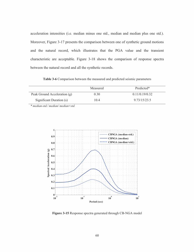
60
acceleration intensities (i.e. median minus one std., median and median plus one std.).
Moreover, Figure 3-17 presents the comparison between one of synthetic ground motions
and the natural record, which illustrates that the PGA value and the transient
characteristic are acceptable. Figure 3-18 shows the comparison of response spectra
between the natural record and all the synthetic records.
Table 3-6 Comparison between the measured and predicted seismic parameters
Measured Predicted*
Peak Ground Acceleration (g) 0.30 0.11/0.19/0.32
Significant Duration (s) 10.4 9.73/15/23.5
* median-std./ median/ median+std.
Figure 3-15 Response spectra generated through CB-NGA model
10-2
10-1
100
101
0
0.1
0.2
0.3
0.4
0.5
0.6
0.7
0.8
0.9
1
Period (sec)
Spec
tral
Acc
eler
atio
n (g
)
CBNGA (median-std.)CBNGA (median)CBNGA (median+std.)

61
Figure 3-16 Synthetic ground motion with different duration and PGA
0 5 10 15 20 25 30
-0.3
-0.2
-0.1
0
0.1
0.2
0.3
Acc
eler
atio
n (g
)
Time (sec)
Synthetic Time History - (M=6.7 , D=23 km, Du=14.4 s,median-std. )
Maximum Acc. is 0.103 g at time 5.1 sec
0 5 10 15 20 25 30
-0.3
-0.2
-0.1
0
0.1
0.2
0.3
Acc
eler
atio
n (g
)
Time (sec)
Synthetic Time History - (M=6.7 , D=23 km, Du=20.3 s,median )
Maximum Acc. is -0.174 g at time 7.3 sec
0 5 10 15 20 25 30
-0.3
-0.2
-0.1
0
0.1
0.2
0.3
Acc
eler
atio
n (g
)
Time (sec)
Synthetic Time History - (M=6.7 , D=23 km, Du=23.5 s,median+std. )
Maximum Acc. is -0.294 g at time 4.8 sec

62
Figure 3-17 Comparison between the natural and synthetic record
Figure 3-18 Comparison of response spectra
0 5 10 15 20 25 30-0.4
-0.3
-0.2
-0.1
0
0.1
0.2
0.3
0.4
Acc
eler
atio
n (g
)
Time (sec)
Natural recordSyn. GM (Dura=22.4 s,median+std.)
10-2
10-1
100
101
0
0.5
1
1.5
Period (sec)
Spec
tral
Acc
eler
atio
n (g
)
Natural recordCBNGA (median-std.)CBNGA (median)CBNGA (median+std.)GMs W/ avg. Vs30
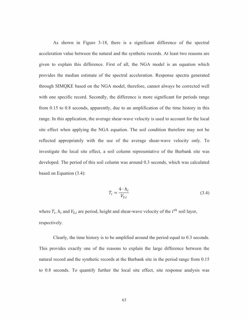
63
As shown in Figure 3-18, there is a significant difference of the spectral
acceleration value between the natural and the synthetic records. At least two reasons are
given to explain this difference. First of all, the NGA model is an equation which
provides the median estimate of the spectral acceleration. Response spectra generated
through SIMQKE based on the NGA model, therefore, cannot always be corrected well
with one specific record. Secondly, the difference is more significant for periods range
from 0.15 to 0.8 seconds, apparently, due to an amplification of the time history in this
range. In this application, the average shear-wave velocity is used to account for the local
site effect when applying the NGA equation. The soil condition therefore may not be
reflected appropriately with the use of the average shear-wave velocity only. To
investigate the local site effect, a soil column representative of the Burbank site was
developed. The period of this soil column was around 0.3 seconds, which was calculated
based on Equation (3.4):
�� � � � ��[>� (3.4)
where ��, �� and [>� are period, height and shear-wave velocity of the o�� soil layer,
respectively.
Clearly, the time history is to be amplified around the period equal to 0.3 seconds.
This provides exactly one of the reasons to explain the large difference between the
natural record and the synthetic records at the Burbank site in the period range from 0.15
to 0.8 seconds. To quantify further the local site effect, site response analysis was

64
performed using the 1-D site response analysis program, DEEPSOIL. Figure 3-19 shows
the comparison of the response spectra between the natural record and the synthetic
records after site response analysis. It is evident that the generated ground motions,
including site response analysis, can represent the actual hazard characterization. Another
time, the importance of the local site effect is emphasized based on the above
investigation.
Figure 3-19 Comparison of response spectra with site response analysis (SR)
3.7.3.2 Application 2—synthetic ground motions with various hazard levels
In this verification, ground motions with various hazard levels were generated
based on the seismic information specified by the users. The deaggregation results for
different hazard levels (10%, 5%, and 2% probability of exceedance in 50 years), as
10-2
10-1
100
0
0.5
1
1.5
Period (sec)
Spec
tral
Acc
eler
atio
n (g
)
Natural recordGMs W/ SR

65
shown in Table 3-7 and Table 3-8, at the Burbank site were fed into this advanced hazard
method. Next, sets of synthetic ground motions, including site response analysis and
varying with duration and hazard levels were generated automatically. These motions
with compatible format were further used in the hybrid simulation and fragility analysis.
Figure 3-20 lists 3 of the 27 generated synthetic ground motions. Rather, Figure 3-21
shows the response spectra in different hazard levels. For completeness, a summary of
the procedure and all the generated ground motions are given in Appendix A.
Table 3-7 Deaggregation results at Burbank site
Return Period (yrs) M R (km) Epsilon
2%/ 50yrs 2475 6.73 6.9 1.18
5%/ 50yrs 975 6.71 8.5 0.91
10%/ 50yrs 475 6.71 10.6 0.63
Table 3-8 Contributed fault information based on deaggregation results
Name Type <7= <AB ����>G �� �Verdugo Char Reverse 1 0 1 0
Elysian Park Char Blind trust (reverse) 1 0 1 0
*assume � = 90°, �)�2 � � �

66
Figure 3-20 Synthetic ground motions for different hazard level and duration
0 5 10 15 20 25-1
-0.8
-0.6
-0.4
-0.2
0
0.2
0.4
0.6
0.8
1
Time (sec)
Acc
eler
tion
(g)
Synthetic Time History -LA_S_2_5
Maximum Acc. is 0.784 g at time 6.8 sec
0 5 10 15 20 25-1
-0.8
-0.6
-0.4
-0.2
0
0.2
0.4
0.6
0.8
1
Time (sec)
Acc
eler
tion
(g)
Synthetic Time History -LA_S_5_5
Maximum Acc. is 0.634 g at time 7.9 sec
0 5 10 15 20 25-1
-0.8
-0.6
-0.4
-0.2
0
0.2
0.4
0.6
0.8
1
Time (sec)
Acc
eler
tion
(g)
Synthetic Time History -LA_S_10_5
Maximum Acc. is 0.614 g at time 7.9 sec

67
Figure 3-21 Response spectra for different hazard level
10-1
100
101
0
0.5
1
1.5
2
2.5
3Synthetic Ground Motions (2%PE/50yrs)
Period (sec)
Spec
tral
Acc
lera
tion
(g)
CB-NGA (median)median+epsilon*std.Syn. GMs.(Bedrock)-avgSyn. GMs. (Surface)-avg.Synthetic Records
10-1
100
101
0
0.5
1
1.5
2
2.5
3Synthetic Ground Motions (5%PE/50yrs)
Period (sec)
Spec
tral
Acc
lera
tion
(g)
CB-NGA (median)median+epsilon*std.Syn. GMs.(Bedrock)-avgSyn. GMs. (Surface)-avg.Synthetic Records
10-1
100
101
0
0.5
1
1.5
2
2.5
3Synthetic Ground Motions (10%PE/50yrs)
Period (sec)
Spec
tral
Acc
lera
tion
(g)
CB-NGA (median)median+epsilon*std.Syn. GMs.(Bedrock)-avgSyn. GMs. (Surface)-avg.Synthetic Records

68
3.7.3.3 Application 3— a site specific hazard map under the Northridge earthquake in
LA area
Hazard map, the exposure when calculating earthquake loss, is one of the
indispensable components of regional impact assessment. The map of PGA for the 1994
Northridge earthquake in the Los Angeles area in standard gravity (g) was generated in
this application. This map is not only served to demonstrate the proposed method, but
also used for regional impact assessment in Los Angeles area, which is presented in
Chapter 6: Case Studies.
SMIP geotechnical report (Fumal et al., 1979) was used again to illustrate local
site characteristics. As mentioned previously, 19 borehole logs are available in SMIP
report. Figure 3-22 shows the locations of these 19 boreholes (black cross) and the
epicenter of the 1994 Northridge earthquake (red star). In order to provide more realistic
site conditions, the Los Angeles area was subdivided into 6 smaller regions, as shown in
Figure 3-23. One of the boreholes in each region was selected to represent the site
condition in that area. Therefore, 6 different site conditions along with earthquake
mechanism of the Northridge earthquake contributed the map of PGA for the 1994
Northridge earthquake in Los Angeles area.
Step-by-step procedures to generate the hazard map (described previoulsy in
section 3.6 Hazard Map Generation) were then performed. The Northridge earthquake
mechanism (Figure 3-10), the site conditions (soil profiles and material properties) and
map information (such as interested region scope and cell size) were defined in the first

69
step. Next, the CB-NGA (Campbell and Bozorgnia, 2008) and duration prediction
equation along with SIMQKE (Gasparini and Vanmarcke, 1976) and DEEPSOIL
(Hashash et al., 2009), were performed for each cell. Finally, PGA values were collected
and hazard map of the Los Angeles area was presented, as shown in Figure 3-24.
Figure 3-22 Locations of boreholes (black cross) in the SMIP geotechnical report
Figure 3-23 Subdivided areas and the selected boreholes in the Los Angeles area
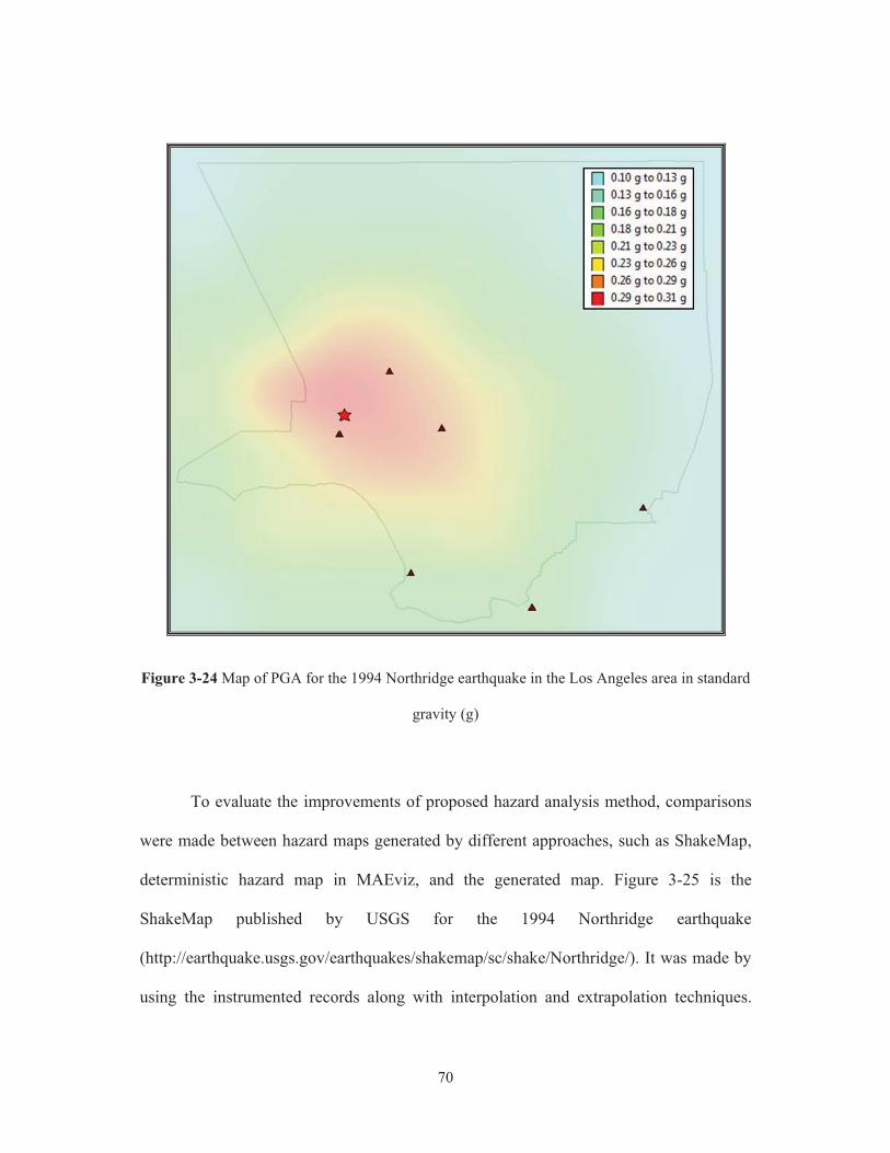
70
Figure 3-24 Map of PGA for the 1994 Northridge earthquake in the Los Angeles area in standard
gravity (g)
To evaluate the improvements of proposed hazard analysis method, comparisons
were made between hazard maps generated by different approaches, such as ShakeMap,
deterministic hazard map in MAEviz, and the generated map. Figure 3-25 is the
ShakeMap published by USGS for the 1994 Northridge earthquake
(http://earthquake.usgs.gov/earthquakes/shakemap/sc/shake/Northridge/). It was made by
using the instrumented records along with interpolation and extrapolation techniques.

71
Therefore, the ShakeMap is relatively realistic. When comparing with ShakeMap, the
generated map is qualititatively reasonable and acceptable.
Figure 3-25 ShakeMap for the 1994 Northridge earthquake (USGS)
(Pink county border is added by the writer)

72
Moreover, a quatitative comaprison was made among ShakeMap, map generated
by MAEviz and map generated by the proposed method (represented by NISRAF in the
following). Figure 3-26 and Figure 3-27 show the generated map as well as differences
between the calculated and the measured PGA values during the 1994 Northridge
earthquake by NISRAF and MAEviz, respectively. Due to the limited site informaiton,
only 6 sites, which were used previously to represent 6 different site conditions, were
discussed here. Generally, the map generated by NISRAF is more reasonable and realistic
than the one from MAEviz. Site response analysis is one reason for this difference—
MAEviz uses a simple approach, the Fa and Fv site coefficients, while NISRAF uses 1-D
site response analysis to account for soil nonlinear behavior.
Between these 6 sites, Tarzana and Sylmar show large differences for both
NISRAF and MAEviz map, even though they have higher estimated PGA values (Table
3-9). Several studies have been devoted to investigate the high PGA values in these two
sites (Hartzell et al., 1996; Vahdani and Wikstrom, 2002). Generally, it is believed that
the local geology and topography, the near-fault, basin and the directivity effect of the
earthquake contribute to the higher response. Among them, topography, near-fault and
directivity effects are not included in current attenuation models and 1-D site response
analysis program.

73
Figure 3-26 Hazard and difference of PGA between NISRAF and measured one
Figure 3-27 Hazard and difference of PGA between MAEviz and measured one

74
Table 3-9 Comparisons of PGA value between the measured and the calculated
PGA (g) Tarzana* Sylmar**
Measured 1.93 0.89
NISRAF 0.29 0.3
MAEviz 0.24 0.2
*Tarzana-Cedar Hill Nursery A (CSMIP #24436)
**Sylmar-6-story County Hospital (CSMIP #24763)
3.8 Summary and Discussion
In conclusion, the above three applications demonstrate the methodologies and
procedures of the proposed advanced hazard analysis method, including seismic hazard
analysis, synthetic ground motions, site response analysis and hazard map generation.
The use of instrumentation data provides an opportunity to calibrate the hazard models,
which, therefore, improve the reliability of the hazard characterization used in the further
analyses, such as synthetic ground motion and hazard map generation. Meanwhile, the
incorporation of site response analysis improves the accuracy in synthetic ground
motions as well as in hazard maps. Moreover, the proposed method simplifies tedious
and complicated procedures in each hazard model, solves the compatibility between them,
and provides an interactive interface for ease of use. This advanced method has already
been implemented in NISRAF successfully, which cooperates with other sub-disciplines
toward the purpose to provide more reliable earthquake impact assessment results.
.
75
CHAPTER 4
FRAGILITY ANALYSIS BY HYBRID SIMULATION
4.1 Introduction
Fragility, or vulnerability, presents the probability of reaching or exceeding a
specific performance level under a specific seismic hazard. Fragility curves relate the
effects of seismic hazard to the damage of the structures. Therefore, fragility curves
(sensitivity) along with hazard (exposure) are used to assess earthquake impact on the
built environment.
As discussed in section 2.6: Fragility Analysis, four categories are generally used
to classify fragility curves—empirical fragility curves, judgmental fragility curves,
analytical fragility curves and hybrid fragility curves. Through development in the past
few decades, the fragility analysis has reached its mature state and also has been widely
accepted by the community. Nevertheless, uncertainties and limitations remain for their
own inherent nature (such as scarcity in empirical fragility curves and subjectivity in
judgmental fragility curves) or modeling deficiencies (analytical fragility curves, for
example). Even the hybrid fragility curves have flaws since different uncertainties
sources exist between different types of fragility relationships.
76
4.2 Overview of the Advanced Hybrid Fragility Analysis Method
In order to reduce the uncertainties and to improve reliability, an advanced hybrid
fragility analysis method is proposed. In this approach, fragility is represented by a
lognormal distribution as shown in Equation (4.1) (Wen et al., 2004).
p� � p N�q V �T � � + ��34*�, + j� � � �Rj�S (4.1)
where j and � denote the mean and standard deviation of 34!*� q� ,. If � and q follow
lognormal distributions, then ��� and ��q follow normal distributions and the function
34!*� q� , also follows a normal distribution. This is, therefore, consistent with the
lognormal distribution assumption for � and q , which is commonly assumed for
fragility analysis. The parameter j is expressed as a function of the earthquake intensity
parameter, such as PGA, which is derived through testing in the laboratory. The standard
deviation � represents uncertainties in both demand and capacity in the analysis, which is
from the literature.
As shown in Figure 4-1, through scaling seismic inputs (ground motions), several
tests (hybrid or conventional simulation) are conducted in the laboratory in order to reach
the target structural response. The seismic intensity (PGA, for example) of the scaled
ground motion is then assigned to the mean seismic intensity for current limit state. The
target structural response is defined for different limit states, such as interstory drift angle
(ISDA) of 0.7% for the immediate occupancy limit state for steel moment frame building.

77
Therefore, with j derived from laboratory testing and � from literature, the fragility
relationships is derived through this advanced hybrid manner.
Figure 4-1 Flow chart for the advanced hybrid fragility analysis
4.3 Verification Studies
Fragility curves of three performance limit states (namely, immediate occupancy,
life safety and collapse prevention) for a mid-rise steel moment resisting frame building
in Los Angeles area were generated through hybrid simulation (with calibrated finite

78
element model along with experimental simulation and site specific ground motions) and
dispersions from similar structures found in the literature.
4.3.1 Structural Model and Seismic Input
4.3.1.1 Building Description and Structural Model
A six-story instrumented building in Burbank, California was selected for this
verification. This is a steel moment resisting frame structure, in which the perimeter
frames are the primary lateral load resisting system and the internal frames are only
resisting gravity load. This building was instrumented by California Strong Motion
Instrumentation Program (CSMIP) in 1980 with 13 sensors. A 2-D finite element model
was built in ZEUS-NL (Elnashai et al., 2004) and tuned using the measured structural
responses (Figure 4-2). More descriptions and discussions of this building, as well as
finite element model construction and model updating results, are detailed in Chapter 6:
Case Studies.
Figure 4-2 Analytical model configuration for Burbank building

79
4.3.1.2 Performance Limit State
Three performance limit states are specified in this study, namely, the immediate
occupancy (IO), the life safety (LS) and the collapse prevention (CP). Interstory drift
angles (ISDAs) 0.7%, 2.5% and 5% are assigned to IO, LS and CP performance level,
respectively (FEMA, 2000b).
4.3.1.3 Seismic Input
Ground motions representative of the local hazard characterization are essential in
order to capture the realistic structural response. In addition, various ground motions
should be considered to avoid excessive scaling on them. Excessive scaling is unrealistic
and unreasonable particularly when motion has higher earthquake intensity. Based on the
above considerations, the 27 site specific synthetic ground motions with various hazard
levels, generated for the Burbank sits (Appendix A), were selected as the earthquake
demand in this verification. To avoid excessive scaling, records related to 10%, 5% and
2% probability of exceedance in 50 years hazard level are used to derive fragility curves
for immediate occupancy, life safety and collapse prevention performance limit state,
respectively.
4.3.2 Hybrid Simulation
The calibrated Burbank building model and ground motions from hazard
characterization analysis were used to verify the extension of the hybrid simulation to
fragility analysis as well as the integration of hybrid simulation in earthquake impact
assessment. The calibrated 2-D structure model was divided into two sub-structures,

80
namely, the column (the lower part of the left exterior column at the first floor) and the
frame (the remaining structure). The frame module was simulated using ZEUS-NL
(Elnashai et al., 2004), while the column module—replaced by a small scale aluminum
specimen (Figure 4-3)—was tested in the laboratory.
Figure 4-3 Hybrid simulation with two sub-structures (column and frame)
4.3.2.1 Testing Facility
George E. Brown, Jr. Network for Earthquake Engineering Simulation (NEES)
equipment site in the University of Illinois at Urbana-Champaign, the Multi-Axial Full-
Scale Sub-Structured Testing and Simulation (MUST-SIM) facility is selected as the
experimental facility. The MUST-SIM facility consists of an L-shaped strong wall, three
large loading and boundary condition boxes (LBCBs) and advanced non-contact
measurement systems (Krypton, for example). In addition to the large-scale facility, a
1/5th–scale model laboratory (including wall-floor system, three boxes, and a portable and
self-reacting LBCB) is available for training, for verifying control algorithms and for

81
investigating structural behaviors in small scale. In this study, the portable LBCB
(pLBCB), as shown in Table 4-1 and Figure 4-4, is employed since the tests are a proof-
of-concept study—to demonstrate the extension and integration of hybrid simulation in
fragility analysis and impact assessment, respectively. Therefore, meeting similitude
requirement is not necessary.
Table 4-1 Force and displacement capacities of portable LBCB (Holub, 2010)
Type Axis Capacity Type Axis Capacity
Displacement* (inch)
X �� Rotation* (degree)
X ����YY �� Y �Z�YZ �� Z ����.
Force* (kip)
X �. Moment* (kip-inch)
X ����ZY �� Y �����Z �Z Z ����Z
*Note the values provides here do not reflect interaction amongst the platen DOF. X actuators have a force capacity of �� kips and a displacement capacity of �� inch. Y and Z actuators have a force capacity of ��kips and displacement capacity of �� inch.
Figure 4-4 Portable LBCB at MUST-SIM 1/5th-scale model laboratory
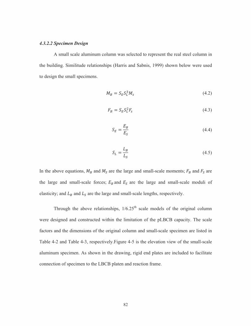
82
4.3.2.2 Specimen Design
A small scale aluminum column was selected to represent the real steel column in
the building. Similitude relationships (Harris and Sabnis, 1999) shown below were used
to design the small specimens.
&M � ��/&� (4.2)
<M � ��)<� (4.3)
� � �M�[ (4.4)
� � M [ (4.5)
In the above equations, &M and &[ are the large and small-scale moments; <M and <[ are
the large and small-scale forces; �M and �[ are the large and small-scale moduli of
elasticity; and M and [ are the large and small-scale lengths, respectively.
Through the above relationships, 1/6.25th scale models of the original column
were designed and constructed within the limitation of the pLBCB capacity. The scale
factors and the dimensions of the original column and small-scale specimen are listed in
Table 4-2 and Table 4-3, respectively.Figure 4-5 is the elevation view of the small-scale
aluminum specimen. As shown in the drawing, rigid end plates are included to facilitate
connection of specimen to the LBCB platen and reaction frame.

83
Table 4-2 Scale factor for design small scale specimen
� �2.9 6.25
Table 4-3 Dimension and material properties of real column and small-scale specimen
d(in)
bf(in)
tw(in)
tf(in)
Elastic modulus E (ksi)
Yield strength fy (ksi)
Real column (W14x184) 15.38 15.66 0.84 1.378 29000 40
Small-scale specimen (Alloy 6061-T6) 3 2.509 0.349 0.26 10000 36
Figure 4-5 Aluminum column specimen elevation, unit: in.

84
(a) Front side view (b) Right side view
Figure 4-6 Completed small-scale specimen
4.3.2.3 Software Environment
4.3.2.3.1 UI-SIMCOR
UI-SIMCOR (Kwon et al., 2007), the University of Illinois software platform for
hybrid simulation, is adopted to coordinate all the sub-structures (modules) during the
testing, such as the communication and interaction between the experimental (column)
and analytical (frame) modules (Figure 4-3). The ¡-Operator Splitting (¡-OS) method is
implemented in UI-SIMCOR to conduct time integration. Generally, three stages, namely,
stiffness evaluation, static loading and dynamic loading are undertaken step by step to
finish a hybrid testing.

85
4.3.2.3.2 ZEUS-NL
The frame sub-structure model was simulated in ZEUS-NL platform (Elnashai et
al., 2004), a nonlinear FE analysis program, developed by the MAE Center. In this
analytical model, section and material properties were based on design documents,
lumped mass was used and applied at each beam-column connection, and concrete slabs
were modeled and connected to steel girders using rigid elements, to account for their
contribution of stiffness. More details about construction of this analytical model are
illustrated in Chapter 6: Case Studies.
4.3.2.3.3 LBCB Operation Manager
The LBCB Operation Manager is a program developed to control the Load and
Boundary Conditions Boxes (LBCB) of MUST-SIM facility. Three control algorithms
are implemented in this program, namely, displacement, force and mixed mode control.
In this study, the displacement control algorithm in Operation Manger is used to control
the portable LBCB during the testing.
4.3.2.3.4 LBCB-Plugin
The LBCB-Plugin was original developed as the intermediary between UI-
SIMCOR and the LBCB Operation Manger. Recently, a new developed LBCB Plugin is
released, which serves as the master program for all the software used during the testing.
Therefore, except the communication between UI-SIMCOR and Operation Manger, this
program synchronizes data collected and pictures taken and stored from data acquisition
program and Camera-Plugin program, respectively.

86
4.3.2.3.5 Data Acquisition
Instrumented data was collected continuously through a custom LabViw program.
In addition to the traditional data (displacement, force and strain), photos were taken
automatically at each time step through Camera-Plugin program developed at MUST-
SIM facility.
4.3.2.4 Experimental Setup
4.3.2.4.1 Testing Configuration
All the small-scale aluminum columns were tested on the portable LBCB. Figure
4-7 presents the experimental setup. As shown in Figure 4-7 (b), the top-end plate of
specimen is attached to the steel frame (fixed end); while the bottom-end plate is attached
to the LBCB platen (flexible (control) end). The control algorithm for this study is based
on the external feedback of linear potentiometers installed on the specimen. Four linear
displacement LVDTs (Liner Variable Differential Transformer) were installed, as shown
in Figure 4-7 (b) (another vertical one is behind the specimen), which provided feedback
on DOF X (in-plane horizontal), Z (vertical) and Ry (out-of-plan rotation). These 3 DOFs
were assigned as the control DOFs in hybrid simulation tests.
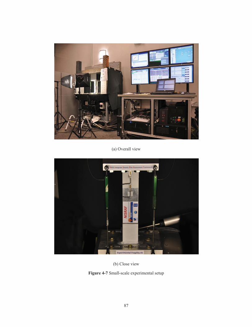
87
(a) Overall view
(b) Close view
Figure 4-7 Small-scale experimental setup

88
4.3.2.4.2 Instrumentation
Six actuator displacements, 6 actuator forces, 6 Cartesian displacements and 6
Cartesian forces from portable LBCB were recorded. Instrumentation from external
measurements was also collected, such as displacements from 4 LVDTs and strain values
from 6 strain gauges. High resolution photos from three angles (namely, front, right and
left side) of the specimen were taken and stored at each time step.
4.3.2.5 Hybrid Simulation Results
Hybrid simulation coordinated by UI-SIMCOR using the Northridge earthquake
record (Figure 4-8) as the ground acceleration was first conducted as a proof test of the
hybrid model prior to the generation of the hybrid fragility curves. As shown in Figure
4-9, good agreement was found between the measured response (CSMIP Station No.
24370 record of the 1994 Northridge earthquake) and the response from the hybrid
simulation testing. With this confidence in the hybrid model and experimental setting, 7
additional hybrid simulation tests with various ground motions were performed in order
to generate the hybrid fragility curves. Details and results of these hybrid simulation tests
are presented in the following section.

89
Figure 4-8 Ground motion record of the 1994 Northridge earthquake (CSMIP # 24370)
Figure 4-9 Comparison of the roof drift between the measured and the hybrid simulation
0 5 10 15 20 25 30 35 40-0.4
-0.3
-0.2
-0.1
0
0.1
0.2
0.3
0.4Input Ground Motions (NR94(EW) - 0.3g)
Time (sec)
Acc
eler
atio
n (g
)
0 5 10 15 20 25 30-5
-4
-3
-2
-1
0
1
2
3
4
5Roof Drift History
Time (sec)
disp
acem
ent (
in)
MeasuredHybrid Simulation

90
4.3.3 Hybrid Fragility Analysis
Based on the lognormal distribution assumption, mean value of seismic intensity
from testing along with dispersions from literature are used to derive the hybrid fragility
curves. In this study, mean value of PGA from hybrid simulation tests and dispersions
from literature (FEMA, 2000a; Cornell et al., 2002; Yun and Foutch, 2000) were used to
derive the fragility curves for this 6-story steel building in Los Angeles area. In the
following section, mean PGA values from hybrid simulation tests are presented first,
followed by discussions on the dispersions found in literature. Moreover, a
comprehensive uncertainty review was also included.
4.3.3.1 Mean PGA Values from Hybrid Simulation
Hybrid simulation results under different synthetic ground motions (10%, 5% and
2% probability of exceedance in 50 years for immediate occupancy, life safety and
collapse prevention performance levels, respectively) were used to derive the mean PGA
value for each performance level. Step-by-step procedure to derive mean PGA value is
given below, also shown in Figure 4-10:
Step 1: 10% probability of exceedance in 50 years ground motion is selected as
seismic input for hybrid simulation to derive mean PGA value for
immediate occupancy limit state.
Step 2: Interstory drift angle (ISDA) is calculated based on testing results.
Comparison of ISDA between the calculated one and the target one (0.7%
ISDA for immediate occupancy performance limit state, for example) is
then made.

91
Step 3: Hybrid simulation is resumed (replaced with new specimen if nonlinear
behavior occurs in previous test) with seismic input multiplied by a scale
factor (calculated based the difference in Step 2), if the difference exceeds
criterion (�5% difference, for example).
Step 4: Iterations from Step1 to Step 3 continues till the criterion is met.
Step 5: Once the calculated ISDA matches the defined ISDA, PGA value of
current (scaled) record is assigned as the mean PGA value for immediate
occupancy performance limit state.
The above procedure is an example of how to drive the fragility curve for IO limit
state, while similar procedures were applied to derive curves for LS and CP limit states
using 5% and 2% probability of exceedance in 50 years ground motions, respectively.
Figure 4-10 Methodology and procedures for the advanced hybrid fragility analysis

92
Figure 4-11 shows the number of hybrid simulation tests used to derive the mean
PGA values. Table 4-4 lists the target ISDA (ISDA, interstory drift angle, are defined in
previous section for this study) as well as the mean PGA values from hybrid simulation
tests.
Figure 4-11 Number of hybrid simulation tests to derive fragility curves
Table 4-4 Interstory drift angle (target ISDA) and PGA from hybrid simulation tests
Performance Level Immediate
Occupancy
Life
Safety
Collapse
Prevention
Interstory drift angle (%) 0.7 2.5 5.0
Mean PGA (g) 0.545 1.627 2.777
Figure 4-13, Figure 4-14 and Figure 4-15 show one simulation result (the red star
highlight with yellow circle area in Figure 4-11, 2% probability of exceedance in 50
0 1 2 3 4 5
0.007
0.025
0.05
Number of Hybrid Simulation
Inte
rsto
ry D
rift A
ngle
Immediate OccupancyLife SafetyCollapse Prevention

93
years multiplied by scale factor equal to 3.54, as shown in Figure 4-12). The other
simulation results can be found in Appendix B.
Figure 4-12 Synthetic Ground motion (2% PE/50yrs with scale factor = 3.54)
Figure 4-13 Comparison of column response between hybrid and multiplatform simulation
0 5 10 15 20 25 30-3
-2
-1
0
1
2
3
Time (sec)
Acc
eler
tion
(g)
Maximum Acc. is 2.777 g at time 6.8 sec
-0.3 -0.2 -0.1 0 0.1 0.2 0.3 0.4 0.5 0.6-1000
-500
0
500
1000
1500Lateral Force v.s. Lateral Displacement
Displacement (in)
Forc
e (lb
)
Hybrid SimulationMultiplatform Simulation
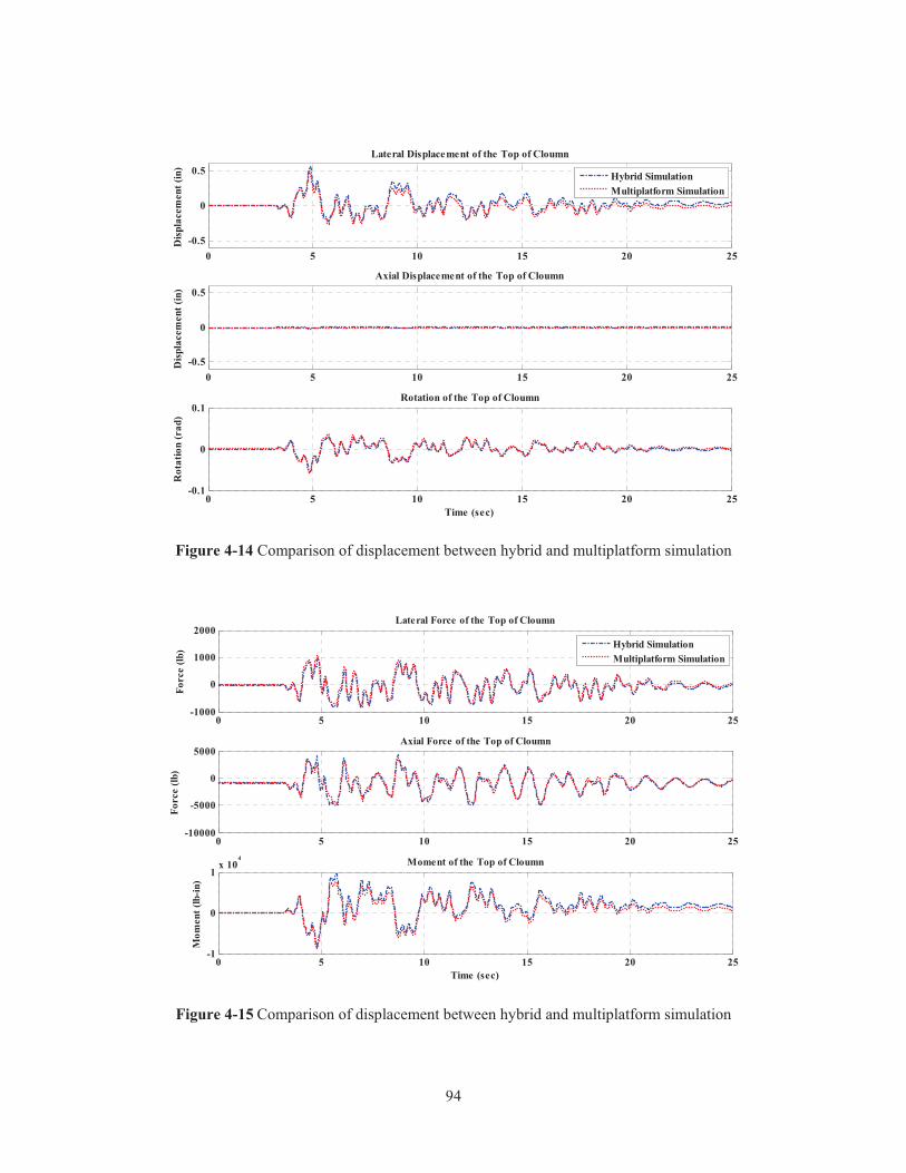
94
Figure 4-14 Comparison of displacement between hybrid and multiplatform simulation
Figure 4-15 Comparison of displacement between hybrid and multiplatform simulation
0 5 10 15 20 25-0.5
0
0.5Lateral Displacement of the Top of Cloumn
Disp
lace
men
t (in
)Hybrid SimulationMultiplatform Simulation
0 5 10 15 20 25-0.5
0
0.5Axial Displacement of the Top of Cloumn
Disp
lace
men
t (in
)
0 5 10 15 20 25-0.1
0
0.1Rotation of the Top of Cloumn
Time (sec)
Rot
atio
n (r
ad)
0 5 10 15 20 25-1000
0
1000
2000Lateral Force of the Top of Cloumn
Forc
e (lb
) Hybrid SimulationMultiplatform Simulation
0 5 10 15 20 25-10000
-5000
0
5000Axial Force of the Top of Cloumn
Forc
e (lb
)
0 5 10 15 20 25-1
0
1x 10
4 Moment of the Top of Cloumn
Time (sec)
Mom
ent (
lb-in
)
95
4.3.3.2 Dispersions from Literature
Dispersion, a statistics vocabulary, represents the uncertainty term in fragility
relationships. Due to the limited number of tests in the hybrid fragility analysis, it is
unreasonable and also unrealistic to regress dispersion based on few testing results.
Therefore, dispersions of the proposed hybrid fragility analysis are found from the
literature.
Generally, uncertainties are divided into two categories, namely, aleatoric and
epistemic uncertainties. Aleatoric uncertainties are inherent, such as occurrence of
earthquakes and material properties (Young’s modulus, yielding strength in steel and
compression strength in concrete, for example). By contrast, epistemic uncertainties are
from the absence of knowledge, such as analytical model selection and construction,
ground motion selection and others) (Wen et al., 2004). Consequently, a comprehensive
review is needed to derive reasonable and representative dispersions.
FEMA 350 (FEMA, 2000a), the recommended seismic design criteria, is specially
developed for new steel moment frame buildings. In FEMA 350, as well as in the
literature (Cornell et al., 2002; Yun and Foutch, 2002), a method used to evaluate seismic
behavior of steel moment frame buildings is proposed. Within this method, uncertainties
for different building height, beam-connection type, analysis procedure (linear or
nonlinear, static or dynamic), and local and global failures under different performance
levels (IO and CP) are tabulated (Table A-3 in FEMA 350) or illustrated in the content.
The uncertainty is therefore calculated using the following equation (Equation (A-4) in
FEMA 350).
96
�8D � ¢£ �¤�)� (4.6)
where �¤� are the standard deviations of the natural logarithms of variation from various
uncertainty sources. Three sources of uncertainties are included, namely, various analysis
methods, beam-column connection behavior and global building stability capacity
prediction. Table 4-5 summaries logarithmic uncertainties for mid-rise steel buildings
obtained from FEMA 350.
Table 4-5 Logarithmic uncertainties for mid-rise building (FEMA, 2000a)
Uncertainty Source Immediate Occupancy Collapse Prevention
Analysis Method* 0.13 0.20
Beam-Column Connection 0.2 0.2
Global Stability Capacity 0.2 0.2
*Nonlinear Dynamic Analysis Method
It is evident that, uncertainties from seismic hazard and material properties are
missing. Although they somehow may be included in the analysis method uncertainty
term, it is unclear here. Meanwhile, uncertainties are available only in two performance
levels; uncertainty for LS is missing.
However, for the proposed advanced hybrid fragility analysis, the above two
missed uncertainties have already been included in the procedures. Uncertainty in seismic
input is captured by using sets of site-specific ground motions and avoiding likely
excessive scale effects. Uncertainty in material properties is covered by calibrating the
FE model in the beginning. Therefore, uncertainties for hybrid fragility curves were
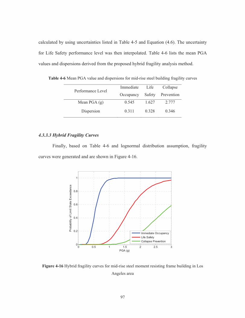
97
calculated by using uncertainties listed in Table 4-5 and Equation (4.6). The uncertainty
for Life Safety performance level was then interpolated. Table 4-6 lists the mean PGA
values and dispersions derived from the proposed hybrid fragility analysis method.
Table 4-6 Mean PGA value and dispersions for mid-rise steel building fragility curves
Performance Level Immediate
Occupancy
Life
Safety
Collapse
Prevention
Mean PGA (g) 0.545 1.627 2.777
Dispersion 0.311 0.328 0.346
4.3.3.3 Hybrid Fragility Curves
Finally, based on Table 4-6 and lognormal distribution assumption, fragility
curves were generated and are shown in Figure 4-16.
Figure 4-16 Hybrid fragility curves for mid-rise steel moment resisting frame building in Los
Angeles area
0 0.5 1 1.5 2 2.5 30
0.2
0.4
0.6
0.8
1
PGA (g)
Pro
babi
lity
of L
imit
Sta
te E
xcee
danc
e
Immediate OccupancyLife SafetyCollapse Prevention

98
A Comparison of fragility relationship between the generated (NISRAF) and the
default fragility curves in MAEviz (the S1M High-Code category, S1M: mid-rise (4-6
stories) steel moment frame) was made and shown in Figure 4-17. As shown, MAEviz
fragility curves are more vulnerable with higher uncertainties. The difference between
them is from different fragility analysis approaches and different seismic inputs. The
MAEviz default fragility relationships are derived analytically (SDOF (single degree of
freedom) dynamic time history analysis). Meanwhile, the ground motions used in
MAEviz are synthetic motions special for Central and Eastern United States (CEUS).
Figure 4-17 Fragility relationship comparison between NISRAF and MAEviz
0 0.5 1 1.5 2 2.5 30
0.2
0.4
0.6
0.8
1
PGA (g)
Pro
babi
lity
of L
imit
Sta
te E
xcee
danc
e
Imm
edia
teO
ccup
ancy
Life Safet
y
CollapsePrevention
NISRAFMAEviz

99
4.4 Fragility Relationships for Other Building Types
A database contained fragility relationships for all building types is an essential
ingredient of regional impact assessment. The proposed advanced hybrid fragility
analysis provides an alternative method to derive more reliable fragility relationships.
Definitely, this hybrid approach can be applied to any other building types. However,
considerable time and effort are required. For the mid-rise steel moment resisting frame
building in Los Angeles area, its fragility relationships have been generated in order to
demonstrate fully the hybrid fragility analysis provided in this study. Extension of the
database for fragility relationships to other building types is underway although it is out
of the scope of this study. Currently, an alternative method to derive fragility
relationships for other building types is the Parameterized Fragility Method, PFM (Jeong
and Elnashai, 2006). In the following section, PFM is reviewed first, followed by the
derivation of fragility relationships for other building types using PFM.
4.4.1 Parameterized Fragility Method
Parameterized Fragility Method (Jeong and Elnashai, 2006), an analytical fragility
analysis approach, derives fragility curves through dynamic time history analysis on a
SDOF FE model. It is, therefore, parameters corresponded with structure types and
ground motions representative of site hazard characterization are essential for this
methodology’s use in regional impact assessment.
In HAZUS-MH, 36 building types (from W1: wood, light frame to MH: mobile
homes) are defined (FEMA, 2006). Meanwhile, structural parameters (period, yield and

100
ultimate strength) for 36 building types under 4 code levels (pre-code, low-code,
moderate-code and high-code) are tabulated. However, the majority of these parameters
are based on engineers’ opinions and experts’ judgment. To be more realistic and
reasonable, the latest research findings on structural capacity are incorporated. For
example, parameters for wood frame and unreinforced masonry buildings are replaced
according to the more comprehensive investigations (Gencturk and Elnashai, 2008;
Frankie, 2010).
In addition, sets of site specific ground motions (Appendix A) are used as
earthquake demand when performing dynamic time history analysis in PFM.
4.4.2 Fragility Relationships for Los Angeles area
Consequently, fragility relationships for 36 building types under 4 code levels
particularly for the Los Angeles area were generated based on structural parameters and
ground motions discussed in previous section. Procedure and results of using PFM to
derive fragility relationships for other building types are detailed in Appendix C. Figure
C-2 tabulates structural fragility parameters for all building types. Comparisons for S1M,
W-series (wood frame) and URM-series (unreinforced masonry building) between
different approaches were made and discussed below.
Figure 4-18 shows comparison of S1M (High-Code) fragility relationships. It is
evident that fragility relationships from PFM are more vulnerable than that from NISRAF,
but less vulnerable than that from MAEviz. SDOF dynamic time history analysis is used
to derive fragility relationships in both PFM and MAEviz, the only difference between

101
them is the seismic inputs. Synthetic motions for the Los Angeles area are used in PFM,
while synthetic motions for CEUS are used in MAEviz. Therefore, the difference
between curves results from seismic inputs. The importance of seismic inputs is therefore
emphasized again.
Figure 4-18 Comparison of S1M (High-Code) fragility relationships
Figure 4-19 and Figure 4-20 show comparison of W1 (wood, light frame), High-
Code and URMM (mid-rise, unreinforced masonry building), Pre-Code between PFM
and MAEviz. Clearly, fragility relationships in PFM are more vulnerable in both W1 and
URMM. In addition to the different seismic input, structural parameters in PFM are
updated by the latest research instead of using parameters listed in HAZUS-MH, which is
in MAEviz. The observation of more vulnerable behavior in both wood frame and
0 0.5 1 1.5 2 2.5 30
0.2
0.4
0.6
0.8
1
PGA (g)
Pro
babi
lity
of L
imit
Sta
te E
xcee
danc
e
Imm
edia
teO
ccup
ancy
Life S
afety
CollapsePrevention
NISRAFPFMMAEviz
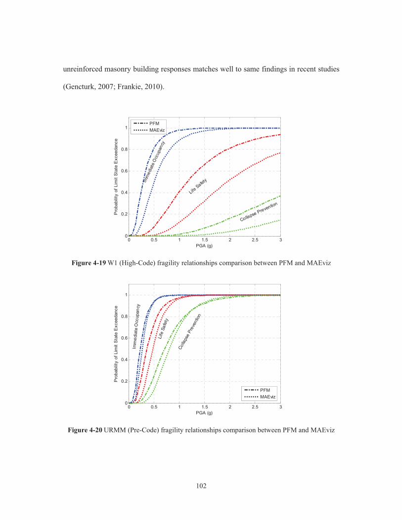
102
unreinforced masonry building responses matches well to same findings in recent studies
(Gencturk, 2007; Frankie, 2010).
Figure 4-19 W1 (High-Code) fragility relationships comparison between PFM and MAEviz
Figure 4-20 URMM (Pre-Code) fragility relationships comparison between PFM and MAEviz
0 0.5 1 1.5 2 2.5 30
0.2
0.4
0.6
0.8
1
PGA (g)
Pro
babi
lity
of L
imit
Sta
te E
xcee
danc
e
Imm
edia
teO
ccup
ancy
Life Safety
Collapse Prevention
PFMMAEviz
0 0.5 1 1.5 2 2.5 30
0.2
0.4
0.6
0.8
1
PGA (g)
Pro
babi
lity
of L
imit
Sta
te E
xcee
danc
e
Imm
edia
teO
ccup
ancy
Life
Safe
ty
Colla
pse
Prev
entio
n
PFMMAEviz
103
4.5 Summary and Discussion
In conclusion, fragility relationships for a steel moment resisting frame building
in the Los Angeles area are developed, which demonstrates the methodologies and
procedures of the proposed advanced hybrid fragility analysis method, including the
incorporation of hybrid simulation into fragility analysis and uncertainty consideration.
The incorporation of hybrid simulation test provides a chance to capture real structural
responses, which therefore improves the reliability of the fragility relationship.
Meanwhile, the comprehensive consideration of uncertainties increases the confidence
when using the generated fragility relationships. Moreover, fragility relationships for 36
building types under 4 code levels in the Los Angeles area are provided by combining the
generated hybrid fragility relationships (S1M, High-Code) with others through PFM
method. In the future, when more and more experimental data are available, fragility
relationships can continue being updated and improved through Bayesian method or
other statistic approaches.
Finally, this advanced hybrid method to derive fragility relationships has already
been implemented in NISRAF successfully, which cooperates with other sub-disciplines
toward the purpose to provide more reliable earthquake impact assessment results.
.

104
CHAPTER 5
DEVELOPMENT OF NEES INTEGRATED SEISMIC RISK
ASSESSMENT FRAMEWORK
5.1 Introduction
NEES Integrated Seismic Risk Assessment Framework (NISRAF), a completed
MATLAB (The MathsWork, Inc.) GUI-driven software platform, has been developed for
the purpose of making impact assessment more efficient and more reliable. Several
components—instrumentation, advanced hazard characterization, system identification,
model updating, hybrid simulation, advanced hybrid fragility analysis and impact
assessment tool—have been implemented and tailored with novel methods to build the
seamless, transparent and extensible framework. Below, the architecture, methodologies,
communication protocols and analysis platforms of NISRAF are discussed first. Next, the
discussions are focused on features, potentials, limitations and challenges of NISRAF.
5.2 Architecture of NISRAF
As shown in Figure 1-2 and Figure 5-1, free-field measurements (I1) along with
nonlinear site response analysis (SR) are used to generate the advanced hazard map and
ground motion records (AH). The measured and synthetic records are then used in hybrid
simulation and fragility analysis. Meanwhile, the structural model is calibrated with the
measured structural response (I2). Next, hybrid simulations (HS) are performed with the

105
most critical component of the structural system tested in the laboratory and the
remainder of the structure simulated analytically. These simulations are conducted to
derive the mean seismic intensity value (PGA, for example) of the corresponding
performance limit state. The fragility curves (FA) of the structure are then generated
using the hybrid simulation data and the dispersions from the literature. Finally, the
hybrid fragility curves and the calibrated hazard map are fed into the impact assessment
tool, such as MAEviz or HAZUS-MH (IA).
Figure 5-1 Architecture of NISRAF

106
Clearly, NISRAF is composed of five main parts: namely, (i) instrumentation (I1,
I2), (ii) seismic hazard analysis (AH), (iii) model calibration and hybrid simulation (HS),
(iv) fragility analysis (FA) and (v) earthquake impact assessment (IA). For ease of use,
nine main menus with submenus are designed and arranged, following the analysis
sequences (Figure 5-2):
� File: Contains general menus (such as Open, Save, Save As, Page Setup,
Print Review, Print and Exit).
� Strong Motion: Provides an interface to download measured data from
instrumentation databases (ANSS, COSMOS, CESMD and PEER).
� Hazard Characterization: Contains three menus (Seismic Hazard Analysis,
Synthetic Time Histories and Hazard Map Generation) to perform hazard
analysis.
� Structure Model: Contains five menus (Import from ZEUS File, New
Model from Template, New Model, View and Structure Model) to import,
develop and view the FE model.
� Model Calibration: Contains three menus (Modal Analysis, System
Identification and Model Updating) to improve the FE model.
� Hybrid Simulation: Contains five menus (Dynamic Load, Static Load,
Hybrid Model, Simulation and Results) to develop the hybrid model, run
simulation and check results.

107
� Fragility Analysis: Contains three menus (Define Limit States, Run
Hybrid Simulation and Hybrid Fragility Curves) to derive hybrid fragility
relationships through hybrid simulation testing.
� Impact Assessment: Contains two menus (MAEviz and HAZUS) to
perform the earthquake impact assessment.
� Help: Contains three menus (NISRAF Manual, UI-SIMCOR Manual,
SimBuild Manual and About NISRAF) to assist users in performing the
analysis. Copyright and version information are also included here.
Figure 5-2 Welcome window and main window of NISRAF
In NISRAF, each main menu is modularized. Moreover, each method and
algorithm implemented in sub-menu is also developed in module unit. This module
feature makes it easy to understand analysis algorithms as well as to maintain this
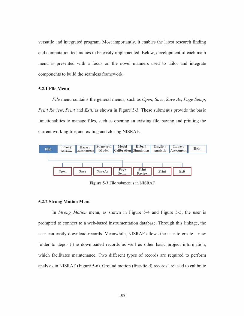
108
versatile and integrated program. Most importantly, it enables the latest research finding
and computation techniques to be easily implemented. Below, development of each main
menu is presented with a focus on the novel manners used to tailor and integrate
components to build the seamless framework.
5.2.1 File Menu
File menu contains the general menus, such as Open, Save, Save As, Page Setup,
Print Review, Print and Exit, as shown in Figure 5-3. These submenus provide the basic
functionalities to manage files, such as opening an existing file, saving and printing the
current working file, and exiting and closing NISRAF.
Figure 5-3 File submenus in NISRAF
5.2.2 Strong Motion Menu
In Strong Motion menu, as shown in Figure 5-4 and Figure 5-5, the user is
prompted to connect to a web-based instrumentation database. Through this linkage, the
user can easily download records. Meanwhile, NISRAF allows the user to create a new
folder to deposit the downloaded records as well as other basic project information,
which facilitates maintenance. Two different types of records are required to perform
analysis in NISRAF (Figure 5-6). Ground motion (free-field) records are used to calibrate

109
hazard models, while structural measurements are used to calibrate structural models.
The incorporation of the instrumented data into NISRAF is not only to increase its usage,
but also to improve hazard and structural model.
Figure 5-4 Schematic of Strong Motion menu in NISRAF
Figure 5-5 Strong Motion menu in NISRAF

110
Figure 5-6 Strong motion data GUI in Strong Motion menu
5.2.3 Hazard Characterization Menu
Hazard characterization menu is composed of three main parts: namely, Seismic
Hazard Analysis, Synthetic Time Histories and Hazard Map Generation, as shown in
Figure 5-7. Methodologies and analysis procedures of hazard characterization analysis
have already been illustrated and verified in Chapter 3: An Advanced Hazard
Characterization Analysis Method. One of the features of the proposed advanced hazard
analysis approach is its ease of use. By tailoring the hazard models as well as ensuring
connection and compatibility between them, it simplifies the complicated and tedious
procedures in the conventional analysis. Consequently, with an interactive interface to
define inputs, hazard analysis becomes efficient and straightforward. Below, analysis
procedures in the three submenus are presented with GUIs and illustrations.

111
Figure 5-7 Hazard Characterization submenu in NISRAF
5.2.3.1 Seismic Hazard Analysis
Two hazard analysis approaches for natural records are available, namely, surface
motions and bedrock motions, as shown in Figure 5-8. GUI for time history and response
spectrum checking is available each time when the analysis is finished (Figure 5-9). Site
response analysis is required for bedrock motions analysis. As mentioned previously,
DEEPSOIL is implemented as the site response analysis platform. To maintain
consistency and ease of use, a GUI interface for creating a representative soil column
(soil profiles and material properties, for example) is developed (Figure 5-10). With the
input file generated by NISRAF, DEEPSOIL is therefore executed in console mode
without its user interface.

112
Figure 5-8 Seismic hazard analysis GUI in Hazard Characterization menu
Figure 5-9 Time history and response spectrum checking GUI

113
Figure 5-10 Define soil profiles and material properties GUI in NISRAF
5.2.3.2 Synthetic Time Histories
Synthetic time history is essential for seismic engineering, particularly in regions
where natural records are absent or insufficient. SIMQKE is the platform implemented in
NISRAF to generate artificial motions. Again, for ease of use, parameters needed for
SIMQKE are generated using the latest attenuation and duration equations (detailed in
Chapter 3) through an interactive interface (Figure 5-11). Meanwhile, a GUI for
customizing the time history is also developed (Figure 5-12). After that, NISRAF
generates the input file (based on user inputs or results from hazard models) and executes
SIMQKE in the console mode (Figure 5-13). Eventually, sets of synthetic ground
motions are generated and are ready for check or use (Figure 5-14).

114
Figure 5-11 GUI to define seismic parameters
Figure 5-12 GUI to customize synthetic time history
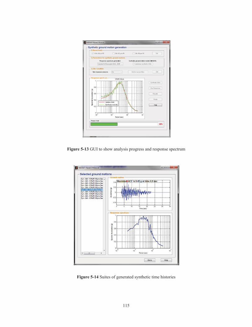
115
Figure 5-13 GUI to show analysis progress and response spectrum
Figure 5-14 Suites of generated synthetic time histories

116
5.2.3.3 Hazard Map Generation
Similar to the case of procedures for synthetic time histories generation, the user
is prompted to specify seismic information in the beginning. Additional information (the
interested area and the cell size used in map) particular to hazard map generation is then
needed to be specified (Figure 5-15). After that, NISRAF calculates seismic intensity
(PGA, for example) at the center of each cell (Figure 5-16). Eventually, a hazard map is
generated by collecting results at each cell along with location information (Figure 5-17).
Figure 5-15 GUI to specify information for hazard map generation

117
Figure 5-16 Hazard map generation in NISRAF
Figure 5-17 Hazard map generated by NISRAF
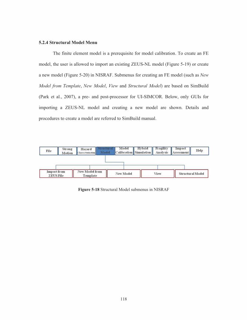
118
5.2.4 Structural Model Menu
The finite element model is a prerequisite for model calibration. To create an FE
model, the user is allowed to import an existing ZEUS-NL model (Figure 5-19) or create
a new model (Figure 5-20) in NISRAF. Submenus for creating an FE model (such as New
Model from Template, New Model, View and Structural Model) are based on SimBuild
(Park et al., 2007), a pre- and post-processor for UI-SIMCOR. Below, only GUIs for
importing a ZEUS-NL model and creating a new model are shown. Details and
procedures to create a model are referred to SimBuild manual.
Figure 5-18 Structural Model submenus in NISRAF

119
Figure 5-19 Imported ZEUS-NL model in NISRAF
Figure 5-20 NISRAF allows user to create FM model

120
5.2.5 Model Calibration Menu
An automatic approach for system identification and model updating is developed
and incorporated into NISRAF. Methodology, procedures and GUIs of this method are
developed by Jian Li at the University of Illinois (Li et al., 2009). Below, brief
introduction of this method is given. A more comprehensive illustration is available in
Appendix D.
As shown in Figure 5-21, Eigensystem Realization Algorithm (ERA) is
implemented in NISRAF due to its wide application and good performance in multi-input
multi-output (MIMO) problems (Figure 5-22). Additionally, the modal updating tool
implemented in NISRAF is featured by its integration with the finite element modeling
capability of NISRAF. Therefore, NISRAF can collect all structural parameters
automatically for the user to select as candidate parameters. Moreover, the objective
function can be customized by defining different numbers of modes and different
weighting factors for frequency and mode shape (Figure 5-23).
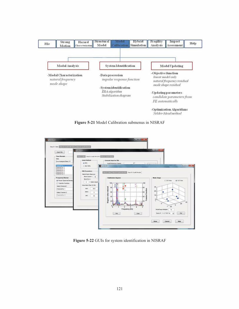
121
Figure 5-21 Model Calibration submenus in NISRAF
Figure 5-22 GUIs for system identification in NISRAF

122
Figure 5-23 GUIs for model updating in NISRAF
5.2.6 Hybrid Simulation Menu
UI-SIMCOR is implemented in NISRAF to coordinate hybrid simulation tests.
The selected ground motions from Hazard Characterization and the calibrated structural
model from Model Calibration are fed into UI-SIMCOR to perform the hybrid simulation.
The GUIs of Hybrid Simulation are based on SimBuild. Through the use of GUIs, the
user can easily develop the sub-structures for the analytical platform or laboratory (Figure
5-25), run hybrid simulation (Figure 5-26) and check results.

123
Figure 5-24 Hybrid Simulation submenus in NISRAF
Figure 5-25 GUIs to define sub-structures in NISRAF

124
Figure 5-26 GUIs to run hybrid simulation in NISRAF
5.2.7 Fragility Analysis Menu
Fragility Analysis menu is composed of three main parts: namely, Define Limit
States, Run Hybrid Simulation and Hybrid Fragility Curves, as shown in Figure 5-27.
Methodologies and analysis procedures of fragility analysis have already been illustrated
and verified in Chapter 4: Fragility Analysis by Hybrid Simulation. One of the features of
the proposed advanced fragility analysis approach is its ease of use. With structural
information available from Structural Model, the user defines interested Interstory drift
angle (ISDA) through the interactive structural model (Figure 5-28). Meanwhile, when
performing hybrid simulation in order to derive mean seismic intensity, NISRAF
calculates ISDAs, compares with target ISDA, calculates scale factor, and asks to

125
continue the next simulation (Figure 5-30). The above designs avoid the heavy and
tedious calculations. The “hold on” feature allows the user to have time to replace the
experimental specimen in the laboratory, which is really a useful and practical design
(Figure 5-30). Eventually, fragility relationships compatible with MAEviz are generated
(Figure 5-31).
Figure 5-27 Fragility Analysis submenus in NISRAF
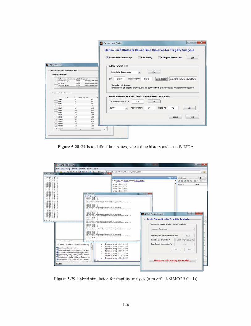
126
Figure 5-28 GUIs to define limit states, select time history and specify ISDA
Figure 5-29 Hybrid simulation for fragility analysis (turn off UI-SIMCOR GUIs)

127
Figure 5-30 GUI to calculate ISDA, scale factor and ask for testing
Figure 5-31 Hybrid fragility curves in NISRAF

128
5.2.8 Impact Assessment Menu
Finally, fragility curves from Fragility Analysis and the hazard map from Hazard
Characterization are fed into earthquake impact assessment packages (MAEviz, for
example) to evaluate the seismic loss (Figure 5-33).
Figure 5-32 Impact Assessment submenus in NISRAF
Figure 5-33 Impact assessment (MAEviz) in NISRAF

129
5.2.9 Help Menu
Manuals of NISRAF, UI-SIMCOR and SimBuild are available. In addition, help
information is also available in each GUI with a button embedded. Moreover, About
NISRAF states the copyright as well as version information.
Figure 5-34 Help submenus in NISRAF
5.3 Communication Protocols and Analysis Platforms
NISRAF, a complete GUI-driven system, has been successfully developed in the
MATLAB environment. The integration from measured data to impact assessment
package is the most important feature of NISRAF. Several different analysis platforms,
such as UI-SIMCOR, ZEUS-NL, DEEPSOIL, SIMQKE and MAEviz are coordinated by
NISRAF to work seamlessly in a single MATLAB platform. No special challenges and
limitations for the communication are observed between components. Moreover, a stand-
alone version NISRAF will be released later. Users do not even need to have MATLAB
installed in their computers to run NISRAF.

130
5.4 Features of NISRAF
NISRAF, an earthquake impact assessment platform with graphical user interface
has been developed for the purpose to make assessment more efficient and more reliable.
Several components, including instrumentation, hazard characterization, system
identification, model updating, hybrid simulation, hybrid fragility analysis and impact
assessment tool, have been implemented and tailored with novel methods to build the
seamless, transparent and extensible framework. Figure 5-35 shows some GUI
components developed and implemented in NISRAF.
Figure 5-35 Components with GUI in NISRAF

131
There are several advanced features contained in this integrated framework.
Among those features are:
� Open source software with friendly graphic user interface:
In NISRAF, each component is developed separately (modularized) before being
incorporated into the framework. Consequently, it is easy to understand and maintain.
This software, as well as the source code, will be open to the public. The open source
feature will allow NISRAF to be utilized efficiently, as well as improve its integrity and
robustness.
� Extensible and accessible:
As mentioned previously, each component is developed and verified separately.
Hence, it is extensible and accessible to any latest research findings and program
techniques.
� Efficient and reliable impact assessment:
This is the first time that all the components for impact assessment are integrated
and work seamlessly in just one software platform. Concurrently, the integrated feature
brings the most advanced tools of earthquake hazard and structural reliability analyses
into the context for accurate evaluation of impact assessment. Surely, with these
seamlessly integrated advanced techniques, which provide a more accurate hazard and
structural model and hence generate superb fragility curves, the assessment of earthquake
impact will be more efficient and more reliable.

132
5.5 Potentials, Limitations and Challenges
As mentioned previously, this is the first time to integrate all components of
earthquake impact assessment in one analysis platform. Through NISRAF, uncertainties
from hazard and fragility can be reduced or managed efficiently; therefore the results
from impact assessment can be more realistic and reliable. Meanwhile, NISRAF provides
a chance for seismologists, geotechnical and structural earthquake engineers, structural
control and impact assessment experts to ameliorate algorithms in order to bring out more
confident assessment results. Through its extensible and accessible feature, the new or
improved algorithm can be easily incorporated into NISRAF.
Despite the above merits, limitations and challenges remain for the current
version NISRAF. First of all, a representative FE structural model is prerequisite and
essential for model calibration. Currently, it is allowed to build the model in NISRAF
(with limited elements, sections and material); and only ZEUS-NL file is compatible
when importing an existing model. However, the model is sometimes too complicated to
be built in NISRAF, or it has already been built in other programs, such as OpenSees and
SAP2000. Furthermore, several analysis platforms have already been implemented in
NISRAF; and it should be expanded in the future. Some of them are operated only by
their own GUIs (such as Java, C++ and others). It is therefore an obstacle when
incorporating into NISRAF. A current alternative method is to prepare the required files
and execute programs in the console modes. To be more robust, and more user-friendly,
the above limitations and challenge should be resolved in the future.

133
CHAPTER 6
CASE STUDIES
6.1 Introduction
NISRAF has been successfully developed, as discussed in Chapter 5. Several
components (modules) in NISRAF have also been verified already, as illustrated in
Chapter 3 and Chapter 4. In this chapter, a verification study of NISRAF is conducted
through an actual test bed in the Los Angeles area. Two applications are presented in this
chapter. In application 1, a heavily instrumented building along with high-quality strong-
motion records was used to demonstrate the methodology and analysis procedure of
NISRAF from instrumentation, testing, to loss assessment. Comparison was made
between the seismic loss through NISRAF and the field reports of the 1994 Northridge
earthquake. Moreover, in application 2, seismic assessment for the Los Angeles area
during the Northridge earthquake was performed using a hazard map and fragility curves
generated by NISRAF; comparison was also presented.
6.2 Application 1: A 6-Story Steel Building in Burbank, California
An instrumented building was selected to verify NISRAF in this application. In
the following sections, background information about this building and site conditions are
presented first. Thereafter, step by step analysis in NISRAF is performed. Comparison is
made and presented in the end.

134
6.2.1 Introduction
6.2.1.1 Building Information
A six-story commercial building in Burbank, California (latitude = 34.185°,
longitude = -118.308°), was selected for this study (Figure 6-1). This is a steel moment
resisting frame building, in which the perimeter frames are the primary lateral load
resisting system, and the internal frames are only resisting gravity load, as shown in
Figure 6-2. Reference is made to Anderson and Bertero (1991) for detailed information
about this building. This building is instrumented by the California Strong Motion
Instrumentation Program (CGS - CSMIP Station No. 24370) in 1980 with 13 sensor
channels as shown in Figure 6-3. Several significant earthquakes were captured, such as
Whittier (1987), Sierra Madre (1991) and Northridge (1994). Data are available in the
Center for Engineering Strong Motion Data (CESMD, www.strongmotioncenter.org).
Figure 6-1 Photo of 6-story steel moment frame building in Burbank, California
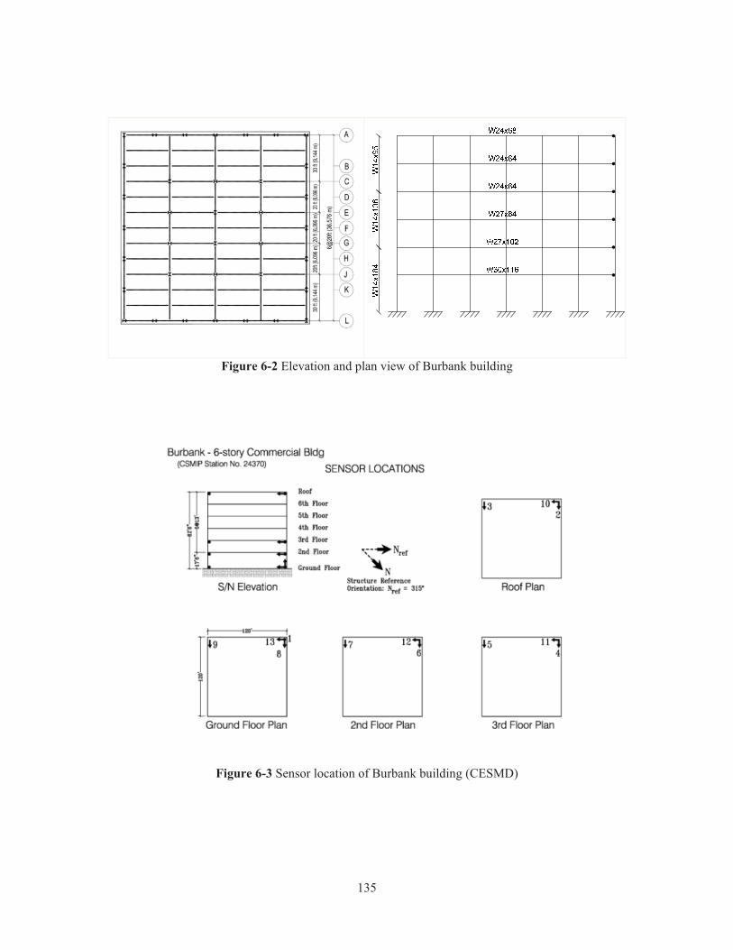
135
Figure 6-2 Elevation and plan view of Burbank building
Figure 6-3 Sensor location of Burbank building (CESMD)

136
6.2.1.2 Site Condition
Site condition of the Burbank Fire Station (latitude = 34.185°, longitude = -
118.308°), the same site utilized in Chapter 3, was selected to represent the site condition
at the Burbank building site due to the absence of geotechnical report at this building site.
This substitution is acceptable since the distance between these two sites is only 0.6
kilometers. Site condition of Burbank Fire Station site has been discussed and detained in
Chapter 3.
6.2.2 Strong Motion
Either Strong Motion or Structural Model must be the first step in NISRAF.
Strong Motion was selected as the first step in this application. Through the linkage to
web-database, free-field station records around the Burbank building site and structural
sensor histories during the past earthquakes were downloaded and deposited in NISRAF.
After that, an interactive window with already-downloaded information allows user to
add some information (background, description and image), as shown in Figure 6-4.

137
Figure 6-4 GUI to manage project and downloaded records
6.2.3 Hazard Characterization
With instrumented strong-motion records from Strong Motion, the hazard
characterization analysis was undertaken. Synthetic ground motions with various hazard
levels were generated for further use in Hybrid Simulation and Fragility Analysis. The
hazard map for the Northridge earthquake in the Los Angeles area was generated for
further use in Impact Assessment. Both of them have already been presented in Chapter 3
and Chapter 4. Figure 6-5 shows the generated synthetic ground motions and hazard map
in NISRAF.

138
(a) Synthetic ground motions (b) Hazard map
Figure 6-5 Synthetic ground motions and hazard map in NISRAF
6.2.4 Structural Model
A finite element model was created in NISRAF, as shown in Figure 6-6. Due to
the fact that only the perimeter frames are used for the lateral load resisting system, a 2-D
model of the exterior frame was modeled to represent the whole structure. Section
dimensions and material properties for each beam and column were based on design
documents. Lumped mass was used and applied at every beam-column connection.
Concrete slabs were modeled and connected to steel girders using rigid elements, to
account for their contribution of stiffness. The width of slab was calculated based on the
effective width defined in ANSI/AISC 360-05 specification (AISC, 2005) and distances
to steel girders were based on design drawings.

139
Figure 6-6 2-D FE model of Burbank building in NISRAF
6.2.5 Model Calibration
With FE model created in Structural Model, Model Calibration is performed to
tune the FE model. Two procedures, namely, system identification and model updating,
were executed in this step.
6.2.5.1 System Identification
Input channels and output channels were defined first in order to form impulse
response functions which were assembled for the Hankel matrix. Based on the design
drawings, exterior and interior columns are firstly supported on steel girders and
reinforced concrete girders, respectively, and both of them are in turn supported on a pair
of 32 feet long and 30 inches diameter reinforced concrete piles. Therefore, it is

140
reasonable to consider that all columns are fixed. Hence, the records from the ground
floor were treated as the input motions, while other records were considered as the
responses of the structure. Consequently, channel 8 and 9 were defined as input, while
channels 2 to 7 were output channels, and, hence, the dimension of impulse function
matrices was 2 by 6. Note that channels 4 and 5 were not working properly during the
Northridge earthquake of 1994. Therefore, data from these two channels were not
available and only four output channels were available. The dimension of impulse
response function matrices was 2 by 4 for the Northridge earthquake.
The ERA method was then performed for the Northridge earthquake record. The
stabilization diagrams and the identified mode shapes were shown in Figure 6-7. The first
and second bending modes were then identified as 0.72 Hz and 2.14 Hz, respectively.
The associated damping ratios were 3.37% and 6.71% (Table 6-1).
Table 6-1 Frequency and ¥ of identified with ERA method
Mode f (Hz) �(%)
1 0.719 3.373
2 2.144 6.715
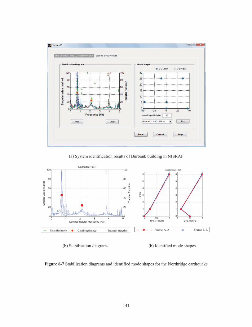
141
(a) System identification results of Burbank building in NISRAF
(b) Stabilization diagrams (b) Identified mode shapes
Figure 6-7 Stabilization diagrams and identified mode shapes for the Northridge earthquake
0 1 2 3 4 50
20
40
60
80
100
Sin
gula
r val
ue re
tain
ed
Damped Natural Frequency (Hz)
Northridge 1994
0 1 2 3 4 50
20
40
60
80
100
Tran
sfer
Fun
ctio
n
Confirmed mode Transfer functionIdentified mode
0 0.5 10
1
2
3
4
5
6
f1=0.71859Hz
Sto
ry
Northridge 1994
-1 0 10
1
2
3
4
5
6
f2=2.1436Hz
Frame L-LFrame A-A

142
6.2.5.2 Model Updating
With the identified natural frequencies and mode shapes, dynamic FE model
updating was then performed to improve the FE model of the Burbank building. Selection
of candidate parameters to be updated was the first step in model updating. The selected
parameters for the Burbank building were shown in Table 6-2. The sensitivities of each
parameter to the first two natural frequencies were shown in Figure 6-8. To keep the
physical meaning of each parameter, lower and upper bounds were applied based on the
degree of uncertainties. For example, the effective widths were calculated based on AISC
specification, which was likely to be very conservative. In addition, the deflection of the
slab defined the contribution of the slab to the composite beam, thus affecting the
effective width. Therefore, the effective width of slab had large uncertainty, thus a
relatively larger range of variation (±50%) was applied.
Table 6-2 Selected parameters for model updating and updated results
Selected
Parameters Description
Initial
Value
Bound
(%)
Updated
Value
Change
(%)
Es (N/mm2) Young’s modulus of steel 2.10E+05 ±5 2.21 E+05 5.00
Mass1 (1000kg) Lumped mass at 2nd floor 45.65 ±5 43.37 -4.99
Mass2 (1000kg) Lumped mass at 3rd-5th floor 36.53 ±5 38.36 5.01
Mass3 (1000kg) Lumped mass at top floor 54.84 ±5 52.1 -5.00
WS1 (mm) Effective width of concrete slab
at 2nd-5th floor 762 ±50 1143 50.00
WS2 (mm) Effective width of concrete slab
at top floor 914.4 ±50 1371 49.93

143
Figure 6-8 Sensitivities of each parameter to the first two identified natural frequencies
The optimization problem defined previously was solved by the Nelder-Mead
method. The results listed in Table 6-3 show that the errors between the identified and
updated model reduced to 1% and 5.78% for the first and second natural frequency,
respectively. Meanwhile, the second mode shape was improved, which gave a value of
0.981 for the MAC. With this refined finite element model, hybrid simulation was
conducted to yield a seismic response prediction with higher accuracy.
Table 6-3 Comparison of frequency and mode shape between the original and updated
Mode
Original FE model Updated FE model
frequency (Hz) MAC
frequency (Hz) MAC
value error (%) value error (%)
1 0.688 -4.312 0.999 0.712 -1.001 0.999
2 1.956 -8.769 0.975 2.020 -5.784 0.981
1 2-0.3
-0.2
-0.1
0
0.1
0.2
0.3
0.4
0.5
Mode Order
Sen
sitiv
ity
EsMass1Mass2Mass3WS1WS2

144
6.2.6 Hybrid Simulation & Fragility Analysis
The calibrated Burbank building model after Model Calibration and ground
motions from Hazard Characterization were used to perform the hybrid simulation and
to derive fragility curves in NISRAF. Both hybrid simulation and hybrid fragility analysis
have already been presented in Chapter 4.
(a) Hybrid simulation model (b) Hybrid fragility curves
Figure 6-9 Hybrid simulation model of Burbank building and the generated fragility curves
6.2.7 Impact Assessment
Finally, with the generated compatible hazard map and fragility curves, MAEviz
under NISRAF was conducted to perform earthquake impact assessment (Figure 6-10).
Table 6-4 lists the probabilities of exceeding limit states. Only 15% probability for
damage occurred in the immediate occupancy limit state. The results met with the post-
earthquake report made by Applied Technology Council (ATC, 2001), which reported
slight damage observed to this building from the Northridge earthquake of (Table 6-5).

145
Figure 6-10 Impact assessment for Burbank building in MAEviz
Table 6-4 Comparison between impact assessment results
Probability of exceeding limit state
Immediate Occupancy Life Safety Collapse Prevention
NISRAF 0.15 0.00 0.00
MAEviz default 0.37 0.04 0.00
Table 6-5 ATC-38 post-earthquake report for the Northridge earthquake of 1994
Building
ID
Number
Model
Building
Type
Number
of
Stories
Design
Date
General
Damage
State
Structural
Damage
State
Nonstructural
Damage
State
… ... … … … … …
CDMG370-MF-09 S1 6 1975 I 1 2
… … … … … … …
*I=Insignificant, M=Moderate
*1=None(0% damage), 2=Slight(0-1%damage), 3=Light (1-10% damage)
*ATC-38, Table A-6 Building Damage Summary for Station CDMG 24370

146
Another comparison of the assessment results was made between NISRAF and
MAEviz default. In MAEviz default, the deterministic hazard and default fragility curves
in MAEviz were used to evaluate seismic loss. Table 6-6 lists the comparison between
these two cases. A comparison of fragility curves between NISRAF and MAEviz default
has also been detailed in Chapter 4, which shows more vulnerability in MAEviz default
fragility relationships (Figure 4-17).
As shown in Table 6-4, assessment results through NISRAF portray less damage
than the results from MAEviz default. Unlike for NISRAF, in which only slight damage
occurs in the immediate occupancy limit state, damage occurs both in immediate
occupancy and life safety limit states for MAEviz default. When comparing with the
ATC-38 report, it is concluded that the assessment result through NISRAF is more
realistic, while the MAEviz default is more conservative.
Table 6-6 Comparison between NISRAF and MAEviz default
NISRAF MAEviz default
Hazard
Deterministic hazard
� Northridge earthquake mechanism
� Campbell and Bozorgnia NGA
� 1-D site response analysis
Deterministic hazard
� Northridge earthquake mechanism
� Campbell and Bozorgnia NGA
� Fa and Fv site coefficients
Fragility
Hybrid fragility relationship
� Calibrated FE model
� Hybrid simulation
� Synthetic motions for LA
Analytical fragility relationship
� SDOF time history analysis
� Synthetic motions for CEUS

147
6.3 Application 2: the Los Angeles area earthquake impact assessment
Earthquake impact assessment on single building provides the possible damage
and loss under scenario or historical earthquake events for this specific building. It indeed
provides valuable information to reduce and mitigate loss in particular for the essential
buildings (hospitals and schools, for example). However, regional impact assessment—
seismic loss for a region, especially urban area—is more valuable for stakeholders to
develop emergency response and recovery planning. In this application, impact
assessment in the Los Angeles area was carried out; comparison was also presented.
6.3.1 Introduction
The Los Angeles area—a high seismic urban region—was selected to demonstrate
the regional impact assessment. Near one million inventory data exported from HAZUS-
MH was used as inventory input. The hazard map of PGA for the Northridge earthquake
in the Los Angeles area and fragility relationships for all building types and code levels
were fed into MAEviz to perform earthquake impact assessment. Both of them have been
generated and fully illustrated in section 3.7.3 Application Examples and section 4.5
Fragility Relationships for Other Building Types, respectively. Therefore, impact
assessment for Los Angeles area under the Northridge earthquake of 1994 was executed;
assessment results were presented with illustrations in the next section.
6.3.2 Assessment Results and Comparison
The MAEviz interface depicted in Figure 6-11 presents the direct economic
building loss for the Los Angeles area in the 1994 Northridge earthquake, using hazard
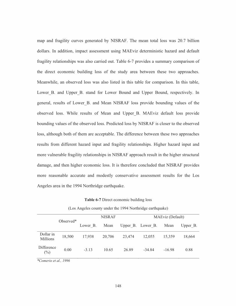
148
map and fragility curves generated by NISRAF. The mean total loss was 20.7 billion
dollars. In addition, impact assessment using MAEviz deterministic hazard and default
fragility relationships was also carried out. Table 6-7 provides a summary comparison of
the direct economic building loss of the study area between these two approaches.
Meanwhile, an observed loss was also listed in this table for comparison. In this table,
Lower_B. and Upper_B. stand for Lower Bound and Upper Bound, respectively. In
general, results of Lower_B. and Mean NISRAF loss provide bounding values of the
observed loss. While results of Mean and Upper_B. MAEviz default loss provide
bounding values of the observed loss. Predicted loss by NISRAF is closer to the observed
loss, although both of them are acceptable. The difference between these two approaches
results from different hazard input and fragility relationships. Higher hazard input and
more vulnerable fragility relationships in NISRAF approach result in the higher structural
damage, and then higher economic loss. It is therefore concluded that NISRAF provides
more reasonable accurate and modestly conservative assessment results for the Los
Angeles area in the 1994 Northridge earthquake.
Table 6-7 Direct economic building loss
(Los Angeles county under the 1994 Northridge earthquake)
Observed* NISRAF MAEviz (Default)
Lower_B. Mean Upper_B. Lower_B. Mean Upper_B.
Dollar in Millions 18,500 17,938 20,706 23,474 12,055 15,359 18,664
Difference (%) 0.00 -3.13 10.65 26.89 -34.84 -16.98 0.88
*Comerio et al., 1996

149
Figure 6-11 Earthquake impact assessment in Los Angeles area
6.4 Uncertainty Analysis in NISRAF
6.4.1 Introduction
Earthquake impact assessment is essential for disaster planning as well as
developing risk reduction policies and emergency responses. As mentioned previously,
an impact assessment package is composed of seismic hazard, fragility function,
inventory data, and integration and visualization capacities. Mathematically, the loss
estimation can be described by the following equation (Ellingwood and Wen, 2005):
p` ¦kka � £££p` ¦kk§r � ¨a � p`r � ¨§ a��[� � p` §©& � ka � p`©& � ka (6.1)
150
where p`ªa is the probability of loss (direct or indirect loss from the earthquake events),
IM is the intensity measure of the seismic hazard (PGA or Sa), and s is the realization of
the intensity measure. p` §©& � ka is the conditional probability of reaching or
exceeding structural limit states, and p`r � ¨§ a is the conditional probability of
reaching damage. Here the term p` §©& � ka refers to fragility or vulnerability
discussed in previous section.
Due to the random nature and limited knowledge in earthquake engineering,
numerous assumptions are made and many approximated methods are applied when
performing impact assessment. Therefore, various types (aleatory and epistemic) of
uncertainties exist in earthquake impact assessment, for example, the prediction of
seismic intensity, the generation of fragility functions, the assumption of distribution of
damage ratio, the inventory uncertainties and others.
With additional investigation and knowledge, it is definitely possible to reduce the
epistemic uncertainties, such as by providing more realistic seismic hazard
characterization, more reliable fragility relationships, and more accurate inventory data.
Nevertheless, uncertainties are unavoidable, particularly in the case of aleatory
uncertainties (randomness). Many approaches (Grossi, 2000; Chang and Song, 2006;
Baker and Cornell, 2008; Elnashai et al., 2009; Choun and Elnashai, 2010) are proposed
to quantify the uncertainties in regional impact assessment, in order to provide
emergency managers and decision makers more confidence when reviewing the
assessment results. Among these proposed approaches, some of them are probabilistic

151
estimations (Baker and Cornell, 2008); while others are approximated approaches (Chang
and Song, 2006; Elnashai et al., 2009; Choun and Elnashai, 2010). In general, the
probabilistic method may need more time and effort for its large computation
requirements. Therefore, the approximated method is relatively more powerful and more
practical for its simple and cost-effective features, in particular for regional impact
assessment.
One advanced feature of MAEviz that distinguishes it from HAZUS-MH is its
uncertainty quantification analysis, which not only provides users with the mean value of
the predicted losses, but also supplies the uncertainty information (the standard deviation
value). With this contribution of uncertainty analysis in MAEviz, NISRAF—to be
consistent with its user-friendly feature—presents the uncertainties through an intuitive
and friendly interface. In the following sections, the methodology of uncertainty
quantification analysis implemented in MAEviz is reviewed briefly, followed by the
demonstration using Los Angeles area earthquake impact assessment results presented
through the developed intuitive interface.
6.4.2 Methodology of uncertainty analysis in MAEviz
The methodology of uncertainty analysis utilized in this study is first proposed by
Chang and Song (2006), which has already been implemented in MAEviz. However,
only mean and standard deviation values are available. Therefore, a program with user-
friendly, intuitive interface is developed and implemented in NISRAF, which allows
users to quantify uncertainties by selecting different confidence intervals. In the

152
following sections, this uncertainty analysis methodology is briefly introduced, followed
by an application to impact assessment results for Los Angeles area under the 1994
Northridge earthquake. More details about this method are referring to the related
reference (Chang and Song, 2006).
6.4.2.1 Uncertainty�in�hazard
Due to many uncertainties, including those related to the site conditions,
earthquake magnitude, and distance to the seismic source, it is difficult to predict the
seismic hazard characterization accurately. To this end, tools for seismic hazard analysis
have been developed in the past decades. Deterministic Seismic Hazard Analysis (DSHA
- Reiter, 1990) and Probabilistic Seismic Hazard Analysis (PSHA - Cornell, 1968) are the
most commonly used methods. For the probabilistic properties and uncertainties from
source, path, and site, uncertainties propagate in the procedure and outcome. To account
for the uncertainties in seismic characterization, an uncertainty term �[� is introduced and
incorporated into the calculation of the fragility curves as shown below:
p� � �� j«�) � �[�) � (6.2)
where j and � are mean and dispersion terms, respectively, when defining
fragility relationships. �[� can be computed using the uncertainty term in NGA model
(Campbell and Bozorgnia, 2008, for example), based on users’ judgment, or from
previous studies (Hays, 1980; Cramer, 2001). Therefore, the generated fragility functions
will be modified before they are ingested into MAEviz to conduct the impact assessment.
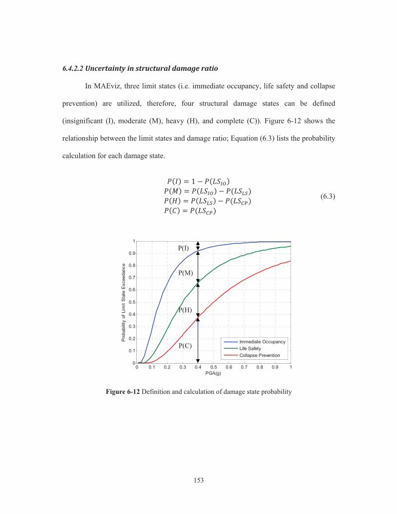
153
6.4.2.2 Uncertainty�in�structural�damage�ratio
In MAEviz, three limit states (i.e. immediate occupancy, life safety and collapse
prevention) are utilized, therefore, four structural damage states can be defined
(insignificant (I), moderate (M), heavy (H), and complete (C)). Figure 6-12 shows the
relationship between the limit states and damage ratio; Equation (6.3) lists the probability
calculation for each damage state.
!!!!!!!!! p*©, � � + p* ¬E,!!!!!!!!!!!!!!!!!!!!!p*&, � p* ¬E, + p* �[,!!!!!!!!!!!!!!!!!!!!!p*, � p* �[, + p* ®9,p*¯, � p* ®9,(6.3)
Figure 6-12 Definition and calculation of damage state probability
0 0.1 0.2 0.3 0.4 0.5 0.6 0.7 0.8 0.9 10
0.1
0.2
0.3
0.4
0.5
0.6
0.7
0.8
0.9
1
PGA(g)
Pro
babi
lity
of L
imit
Sta
te E
xcee
danc
e
Immediate OccupancyLife SafetyCollapse Prevention
P(M)
P(H)
P(C)
P(I)

154
With the probability of each damage state, the total damage of structures after
seismic events is calculated using the probabilities multiplied by the ratio for each
damage state. In MAEviz, the damage ratio proposed by Bai et al. (2009) is utilized to
calculate damage of structures. Table 6-8 lists the mean and standard deviation of the
damage ratio for each damage state.
Table 6-8 Probability model for structural damage ratio (Bai et al., 2009)
Damage states iDS
Range of Beta distribution (%)
Mean of damage ratio
iD DS� (%) Std. of damage ratio
iD DS� (%)
Insignificant [0, 1] 0.5 0.333 Moderate [1, 30] 15.5 9.67
Heavy [30, 80] 55 16.7 Complete [80, 100] 90 6.67
With the above information, the mean and variance of damage ratio (D) are
computed using Equation (6.4).
!!!!!!!!!!!!!!!!�° � £`p*r�, � �°§°[{a1�±%!�°) � �`r)a + �°)
!!!!!!!!!!!!!!!!!!!!!!!!!!!!!!!!!!!!!!!!!!!!!!!!!!!!!� £ep*r�, � ²�°§°[{) � �°§°[{) ³h + �°)1�±%
(6.4)
where p*r�,, i=1,…,4, denotes the combined probabilities of the i-th damage state.

155
6.4.2.3 Uncertainty�in�nonstructural�and�content�damage�ratio
Similar procedures and related probabilistic assumptions are applied to
nonstructural and content damage. Finally, both mean and variance of nonstructural and
content damage ratios can be computed. For more details refer to Chang and Song (2006).
6.4.2.4 Loss�estimation
With the damage ratio for structural, nonstructural and contents, the damage loss
can be computed by Equation (6.5). Equation (6.5) is the loss for one single inventory
only; therefore, the regional seismic loss is calculated by summing up all the inventory
losses in the interested region. Moreover, this approach allows users to include inventory
uncertainty when performing uncertainty analysis, which is detained in Chang and Song
(2006).
¦kk � & � *¡[° � r[° � ¡A[ � rA[ � ¡®� � r®�, (6.5)
where !& is the total cost of the structure; ¡[°!P4µ!¡A[ are the fractions of the total cost
of the structure; ¡®� is the ratio of the contents value to the structural value. r[°> !rA[> P4µ!!r®� are the damage ratio of structural, nonstructural components, and
contents, respectively. Based on Equation (6.5), mean and variance of seismic loss are
estimated by:
!!!!!!!!!!!!!!!!��¶�� � £& � *¡[° � �°·¸ � ¡A[ � �°¹· � ¡®� � �°º»,!!!!!!!!!!!!!!!!!!!!!!��¶��) � £&)e*¡[°,)�°·¸) � *¡A[,)�°¹·) � *¡®�,)�°º») h (6.6)

156
6.4.2.5 Uncertainty�representation
To be more intuitive, the loss uncertainty is quantified using confidence interval
presentation, as shown in Equation (6.7), with (� + ¡,� confidence interval. Log-normal
distribution assumption is made for the seismic loss.
!¯© � ! ec*¼z½¾ f� �¿,> c*¼d½¾ f� �¿,hÀ�c�c j � ��� + ����)� � «��`� � *� �� ,)a (6.7)
where j!P4µ!� are the logarithmic mean � and standard deviation � of the loss,
respectively. Á )� is calculated by Á )� � �d%²� +  �à ³.
6.4.3 Uncertainty analysis in NISRAF
Since the uncertainty analysis method mentioned above has been implemented in
MAEviz, the impact assessment results of MAEviz (only mean and standard deviation
values of structural, nonstructural and contents damage) will be used to quantify the
uncertainty effects by showing different confidence intervals of the assessment results. A
program with an intuitive and user-friendly interface is developed and implemented in
NISRAF to represent the uncertainty quantification analysis. Through this interface, a
pie-chart of different losses (i.e. structural, nonstructural and contents) is presented.
Losses with upper-bound and lower-bound vary with the selection of the confidence level
by the user (Figure 6-13).

157
Figure 6-13 GUI in NISRAF with user-friendly interface for uncertainty quantification
6.4.4 Discussion of Uncertainty Analysis
Due to the random nature of seismic hazard and the limited knowledge and data,
various types of uncertainties are inherent in earthquake loss estimation, from hazard
model, inventory collection, and fragility derivation, to economic loss calculation. These
unquantified uncertainties will result in significant under- or over-estimation of the
assessment results. With the implemented approximate uncertainty quantification
analysis presented through an intuitive way, decision-makers are able to judge the losses

158
easily and quickly, which will help to make more suitable and more confident recovery
plans and emergency responses.
Even though the development and implementation of the proposed uncertainty
quantification analysis method were successful, there are some limitations. Many
investigations are still needed to improve the uncertainty results. For example, the
uncertainty quantification approach is mainly based on many probabilistic assumptions,
for example, the Beta distribution for the damage ratio. More studies are required to
verify this distribution assumption. Also, more research is required to improve our
understanding in earthquake source model, wave propagation, site effect, structural
response, and also more accurate and comprehensive inventory data. With this additional
information, which reduces the uncertainty effects in loss estimation, decision-makers
will surely be more confident with their decisions.
6.5 Summary and Conclusion
The actual test bed in California, the 6-story steel building was carried out to
demonstrate the integrated framework as well as its components. This building example
demonstrated not only the seamlessly-integrated, extensible and transparent framework,
but also that all the elements required for impact assessment can be performed under just
one software platform. Consequently, the impact assessment result, which correlated with
the post-earthquake reports, confirmed one of the advanced features of NISRAF—more
efficient and more reliable impact assessment. Meanwhile, it also proved that the
159
proposed advanced methods—the hazard characterization analysis, the model calibration
and the hybrid fragility analysis—were reliable. As a result of the demonstration of this
impact assessment on one individual building, the same procedures can be extended to
other different building types, seismic code levels and construction materials, to perform
regional impact assessment. In regional impact assessment example, seismic loss through
NISRAF for the Los Angeles area in the Northridge earthquake showed reasonable
accurate, although conservative. Also, the implemented approximate uncertainty
quantification analysis helps decision-makers to judge the losses easily and quickly,
which will help to make more suitable and more confident recovery plans and emergency
responses.

160
CHAPTER 7
CONCLUSIONS AND RECOMMENDATIONS
7.1 Summary of Findings
In this study, a reliable and integrated methodology for earthquake impact
assessment using sensor data, site response analysis, model updating and hybrid
simulation-based fragility analysis is proposed. The methodology is presented through a
software framework, referred to as NISRAF, which supports integrated earthquake
impact assessment for mitigation, emergency response and recovery planning. The
software package is developed and verified in the dissertation. The methodology of
NISRAF is described and its applicability and significance are demonstrated in part
through an application example. In this integrated approach, the hazard characterization
is generated from the measured data, and the structural fragility curves are developed
from the hybrid simulation (with the calibrated numerical model, subjected to the derived
strong-motion records), along with dispersions from the literature. The integration feature
makes use of existing tools in a new approach towards a more efficient and reliable
earthquake impact assessment.
Provided herein is a summary of the major findings stemming from not only the
integrated framework, but also from the component verification studies carried out as part
of the investigation. Also included is the discussion of the contributions and impacts
which NISRAF has made upon the NEES and earthquake engineering communities.

161
The first component verification study, the advanced hazard characterization
analysis module, demonstrates the procedure through which ground motion records are
generated using SIMQKE along with NGA models and the predicted duration. By
utilizing the measured instrumentation along with NGA models and the predicted
duration, and by suitably adjusting SIMQKE, the proposed approach provides engineers
with improved seismic hazard characterization for regional impact assessment. For
example, with the utilization of the measured free-field records to calibrate the hazard
characterization, and attenuation models along with site response analysis to generate
synthetic ground motions, the proposed method surely provides more realistic hazard
characterization than one that is based on mathematical formulations without calibration
with the natural records. Meanwhile, with few seismic parameters being specified, the
proposed approach calculates all required information automatically and produces the
synthetic motions and hazard map efficiently and as accurately as possible.
The second component verification study validates the proposed advanced hybrid
method for fragility curves generation. Hybrid simulation results under different synthetic
ground motions (10%, 5% and 2% probability of exceedance in 50 years for immediate
occupancy, life safety and collapse prevention performance levels, respectively) are used
to derive the mean PGA value for each performance level. Using these mean values,
along with dispersions from previous studies with similar structures, fragility curves are
generated based on the lognormal distribution assumption. This hybrid fragility approach
provides a straightforward and efficient way to derive fragility curves. Hence, this

162
approach is recommended to derive more reliable fragility relationships for other building
types, although it requires time and effort.
Finally, the actual test bed in the Los Angeles area, the 6-story steel building and
the Los Angeles area impact assessment were carried out to verify the integrated
framework as well as its components. The reasonable, although conservative, impact
assessment results not only demonstrated one of the advanced features of NISRAF, that is
making impact assessment more efficient and more reliable, but also highlighted the high
degree of reliability for the new hazard characterization and hybrid fragility methods.
7.2 Ideas for Future Research
The study presented in this dissertation validated the proposed integrated
framework as well as the advanced analysis methods in hazard and fragility. In addition,
the study demonstrated that all the elements required for an accurate impact assessment
can be performed through one software platform. As previously mentioned, the proposed
advanced methods—the hazard characterization analysis, the model calibration and the
hybrid fragility analysis—has proven to be reliable. Nevertheless, due to its inherently
complicated but extensible features, several studies are required to further improve the
accuracy and robustness of NISRAF. Provided below are some suggestions for future
studies:
� To corroborate the concept of the integration of hybrid simulation in NISRAF,
small-scale specimens were used in this study. Additional large-scale hybrid

163
simulation testing is warranted to capture some inherent limitations in small-scale
testing (localized behavior, for example).
� To account for the probabilistic characteristics and uncertainties in hazard
analysis, ‘Logical Tree’ computation scheme is recommended after implementing
additional attenuation models in NISRAF.
� Linear model updating algorithm based on the instrumented data is used to
improve the numerical model in this study. Additional research on nonlinear
model updating algorithms and techniques (such as model updating based on
hybrid simulation results) is essential to improve the structural model and hence
improve fragility curves.
� NISRAF, a versatile and integrated software tool, provides a platform for
earthquake impact assessment and has been developed successfully. Many
analysis algorithms and simulation techniques have also been implemented and
are currently working seamlessly. To increase flexibility and robustness, research
findings and techniques need to be continuously integrated with NISRAF as they
appear in the literature. For example, OpenFresco, the University of California at
Berkeley hybrid simulation software, can be another coordinator for hybrid
simulation; SHAKE91 can be a choice for site response analysis; and HAZUS-
MH can also be used to perform the impact assessment under NISRAF.
� Good agreement was achieved between the estimated and field-observed loss for
the test bed in the Los Angeles area. However, test bed verifications in different
areas for different structural types (highway bridge in Japan and high-technology

164
industry building in Taiwan, for example) are needed. These future verifications
can further validate the methodologies of NISRAF as well as introduce this tool to
research communities worldwide.
� The development of a Web-NISRAF, a Web-based NEES Integrated Seismic
Risk Assessment Framework, is recommended for its potential impact on
collaborative research in earthquake impact assessment. The Web-based feature
could enable users to access NISRAF and perform analysis anytime and at any
place around the world; therefore, it has no limitations in computational capacity.
Moreover, within a unified database, where all simulation data is deposited, users
can access previous data and share their own results efficiently.
7.3 Closure
NISRAF serves as a user-friendly software platform through which impact
assessment can be efficiently and reliably performed by combining hazard (exposure) and
fragility (sensitivity), to provide assessment of impact on the built environment at the
regional scale. Concurrently, it extends the state-of-the-art hybrid simulation approach to
fragility analysis, and proposes novel methods for hazard characterization. The successful
completion of the development of the framework and verification of each component as
well as communication between them, not only demonstrate that these objectives are
achieved, but they also showcase the power and advantages offered by the George E.
Brown, Jr. Network for Earthquake Engineering Simulation (NEES). For example, hybrid
simulation enables NISRAF to integrate testing capabilities at multiple NEES sites. The
165
assessment thereby employs the strength of existing computation models and the
expertise of individual research groups to explore previously unapproachable problems.
Finally, the application of NISRAF will be a stimulus not only to geotechnical and
structural earthquake engineers and impact assessment experts, but also for seismologists
and structural control researchers improving their algorithms in order to pursue the
ultimate goal of NEES under NEHRP: the assessment and mitigation of earthquake losses.

166
REFERENCES
Abrahamson, N. and Silva, W. (2008). “Summary of the NGA Ground-Motion Relations,” Earthquake Spectra, 24(1): 67-98.
AISC (2005). Specification for structural steel buildings, ANSI/AISC 360-05, American Institute of Steel Construction, Inc., Chicago.
Allemang, R. J. and Brown, D. L. (1982). “A Correction Coefficient for Modal Vector Analysis,” Proceedings, International Modal Analysis Conference, Orlando, Florida, 110~116.
Ambraseys, N. N. and Douglas, J. (2003). “Near-field horizontal and vertical earthquake ground motions,” Soil Dynamics and Earthquake Engineering, 23(1): 1-18.
Ambraseys, N. N. and Bommer, J. J. (1991). “The attenuation of ground accelerations in Europe,” Earthquake Engineering and Structural Dynamics, 20(12): 1179-1202
Anderson, J. C., Bertero, V. V. (1991). Seismic performance of an instrumented six-story steel building, Report UCB/EERC-91/11, University of California, Berkeley, U.S.A.
Applied Technology Council (2001). Database on the performance of structures near strong-motion recordings: 1994 Northridge, California, earthquake, Report No. ATC-38, Redwood City, CA.
Bai, J. W., Hueste, M. B. D., and Gardoni, P., (2009), “Probabilistic Assessment of Structural Damage due to Earthquakes for Buildings in Mid-America”, Journal of Structural Engineering, Accepted, May 2009.
Baker, J. W. and Cornell, C. A., (2008), “Uncertainty propagation and feature selection for loss estimation”, Structural Safety, 30(3): 236-252.
Bommer, J. J. and Martinez-Pereira, A. (1999). “The effective duration of earthquake strong-motion,” Journal of Earthquake Engineering, 3(2): 127-172.
Boore, D. M. and Atkinson, G. M. (2008). “Ground-Motion Prediction Equations for the Average Horizontal Component of PGA, PGV, and 5%-Damped PSA at Spectral Period between 0.01 s and 10.0 s,” Earthquake Spectra, 24(1): 99-138.
Boore, D. M., Joyner, W. B., and Fumal, T. E. (1997). “Equations for estimating horizontal response spectra and peak acceleration from western North American earthquakes: A summary of recent work,” Seismological Research Letters, 68(1): 128-153.

167
Calvi, G. M., Magenes, G., Bommer, J. J. Restrepo-Velez, L. F. and Crowley, H. (2006). “Development of Seismic Vulnerability Assessment Methodologies over the Past 30 Years,” ISET Journal of Earthquake Technology, 43(2): 75-104.
Campbell, K. W. (1997). “Empirical near-source attenuation relationships for horizontal and vertical components of peak ground acceleration, peak ground velocity, and pseudo-absolute acceleration response spectra,” Seismological Research Letters, 68(1): 154-179.
Campbell, K. W. and Bozorgnia, Y. (2008). “NGA Ground Motion Model for the Geometric Mean Horizontal Component of PGA, PGV, PGD and 5% Damped Linear Elastic Response Spectra for Periods Ranging from 0.01 to 10 s,” Earthquake Spectra, 24(1): 139-172.
Campbell, K. W. and Bozorgnia, Y. (2007). “Campbell-Bozorgnia NGA Ground Motion Relations for the Geometric Mean Horizontal Component of Peak and Spectral Ground Motion Parameters,” UCB/PEER 2007/02, Pacific Earthquake Engineering Research Center.
Campbell, K. W. and Bozorgnia, Y. (2003). “Updated near-source ground-motion (attenuation) relationships for the horizontal and vertical components of peak ground acceleration and acceleration response spectra,” Bulletin of the Seismological Society of America, 93(1): 314-331.
Chang, F. K. and Krinitzsky, E. L. (1977). “Duration, spectral content and predominant period of strong motion earthquake records from western United States,” Miscellaneous Paper 5-73-1, US Army Corps of Engineers Waterways Experiment Station, Vicksburg, Mississippi.
Chang, L. and Song, J., (2006) “Systematic Treatment of Uncertainty in Consequence-Based Management of Seismic Regional Losses,” Mid-America Earthquake Center, University of Illinois at Urbana-Champaign.
Chen, C. H., Lai, W. C., Cordova, P., Deirelein, G. G., and Tsai, K. C. (2003). “Pseudo-Dynamic Test of Full-Scale Rcs Frame: Part I – Design, Construction and Testing,” Proceedings of International Workshop on Steel and Concrete Composite Constructions, Taipei, Taiwan, 107-118.
Chiou, B. and Youngs, R. (2008). “An NGA Model for the Average Horizontal Component of Peak Ground Motion and Response Spectra,” Earthquake Spectra, 24(1): 173-216.
Choun, Y. -S. and Elnashai, A. S., (2010), “A simplified framework for probabilistic earthquake loss estimation”, Probabilistic Engineering Mechanics, 25(2010): 355-364.
Cmerio, M. C., Landis, J. D., Firpo, C. J. And Monzon, J. P. (1996). “Residential Earthquake Recovery’’ California Policy Seminar, University of California, Berkeley, CA.

168
Cornell, C. A. (1968). “Engineering seismic risk analysis,” Bulletin of the Seismological Society of America, 58(4): 1583-1606.
Cornell, C. A., Jalayer, F., Hamburger, R. O., and Foutch, D. A. (2002). “Probabilistic Basis for 2000 SAC Federal Emergency Management Agency Steel Moment Frame Guidelines,’’ Journal of Structural Engineering, 128(4): 526-533.
Cramer, C. H., (2001), “A seismic hazard uncertainty analysis for the New Madrid seismic zone”, Engineering Geology, 62(1-3): 251-266.
Department of Conservation, Division of Mines and Geology (1998). Seismic hazard zone report for the Burbank 7.5-minute quadrangle, Los Angeles County, California, Seismic Hazard Zone Report 016.
Ellingwood, B. R. and Wen, K. Y., (2005), “Risk-benefit-based design decisions for low-probability/high consequence earthquake events in Mid-America,” Progress in Structural Engineering and Material, 7:56-70.
Elnashai, A. S., Cleveland, L. J., Jefferson T., and Harrald, J., (2009) “Impact of New Madrid Seismic Zone Earthquakes on the Central USA,” Mid-America Earthquake Center Report 09-03, University of Illinois at Urbana-Champaign.
Elnashai, A. S., Elghazouli, A. Y. and Dowling, P. J. (1990). “Verification of Pseudo-Dynamic Testing of Steel Members,” Journal of Constructional Steel Research, Vol. 16, pp. 153-161.
Elnashai, A. S., Papanikolaou V., and Lee, D. (2002). Zeus NL – a system for inelastic analysis of structures, Mid-America Earthquake Center, University of Illinois at Urbana-Champaign, Program Release January 2004.
Federal Emergency Management Agency (2000a). Recommended Seismic Design Criteria for New Steel Moment-Frame Buildings, Report No. FEMA-350, Washington D.C.
Federal Emergency Management Agency (2000b). Prestandard and Commentary for the Seismic Rehabilitation of Building, Report No. FEMA-356, Washington D.C.
Federal Emergency Management Agency (2006). HAZUS-MH technical manual, FEMA, Washington, D.C.
Federal Emergency Management Agency (2009). NEHRP (National Earthquake Hazard Reduction Program) Recommended Seismic Provisions for New Buildings and Other Structures, Report No. FEMA-P-750, Washington D.C.
Filippou, F. C. and Constantinides, M. (2004). FEDEASLab Getting Started Guide and Simulation Examples, Technical Report NEESgrid-2004-22.

169
Frankie, T. M. (2010). Simulation-Based Fragility Relationships for Unreinforced Masonry Buildings, MS thesis, Department of Civil and Environmental Engineering, University of Illinois at Urbana-Champaign, Urbana, Illinois.
Friswell, M. I. and Mottershead, J. E. (1995). “Finite Element Model Updating in Structural Dynamics,” Kluwer Academic Publishers, Dordrecht.
Fumal, T. E., Gibbs, J. F., and Roth, E. F. (1979). In-situ measurements of seismic velocity at 19 locations in the Los Angeles, California region, SMIP geotechnical report No. 131, U.S. Geological Survey.
Gasparini, D. A. and Vanmarcke, E. H. (1976). Simulated Earthquake Motions Compatible with Prescribed Response Spectra, Evaluation of Seismic Safety of Buildings Report No.2, Massachusetts Institute of Technology.
Gencturk, B. E. (2007). Fragility Relationships for Populations of Building Based on Inelastic Response, MS thesis, Department of Civil and Environmental Engineering, University of Illinois at Urbana-Champaign, Urbana, Illinois.
Gencturk, B. E. and Elnashai, A. S. (2008). “Development and application of an advanced capacity spectrum method,” Engineering Structures, 30:3345–3354.
Grossi, P., (2000), “Quantifying the Uncertainty in Seismic Risk and Loss Estimation,” University of Pennsylvania-Electronic Dissertations, Paper AAI9976429, University of Pennsylvania, Philadelphia, Pennsylvania.
Harris, H. G. and Sabnis, G. M. (1999). “Structural Modeling and Experimental Techniques,” CRC Press, Florida.
Hartzell, S., Leeds, A., Frankel, A. and Michael J. (1996). “Site Response for Urban Los Angeles Using Aftershocks of the Northridge Earthquake,” Bulletin of the Seismological Society of America, 86(1B):S168–S192.
Hashash, Y., Groholski, D.R., Phillips, C.A., Park, D. (2009). DEEPSOIL V3.5beta, User Manual and Tutorial.
Hays, W. W., (1980), “Procedures for estimating earthquake ground motions,” US geological survey professional paper 1114. Washington DC.
Hibbit, H. D., Karlsson, B. I., and Sorensen (2001). ABAQUS theory manual. Version 6.2.
Holub, C. J. (2009). Interaction of Variable Axial Load and Shear Effects in RC Bridges, Ph.D. thesis, Department of Civil and Environmental Engineering, University of Illinois at Urbana-Champaign, Urbana, Illinois.

170
Idriss, I. M. (2008). “An NGA Empirical Model for Estimating the Horizontal Spectral Values Generated By Shallow Crustal Earthquakes,” Earthquake Spectra, 24(1): 217-242.
Idriss, I. M. and Sun, J. I. (1992). User’s Manual for SHAKE91, A Computer Program for Conducting Equivalent Linear Seismic Response Analyses of Horizontally Layered Soil Deposits.
Jeong, S. H. and Elnashai, A. S. (2004). “Analytical and Experimental Seismic Assessment of Irregular RC Buildings,” Proceedings of 13th World Conference on Earthquake Engineering, Vancouver, B.C., Canada.
Jeong, S. H. and Elnashai, A. S. (2006). “Probabilistic fragility analysis parameterized by fundamental response quantities,” Engineering Structures., 29:1238-1251.
Juang, J. N. and Pappa, R. S. (1985). “An eigensystem realization algorithm for modal parameter identification and model reduction,” Journal of Guidance, Control, and Dynamics, 8(5): 620-627.
Kawashima, K. and Aizawa, K. (1989). “Bracketed and normalized durations of earthquake ground accelerations,” Earthquake Engineering and Structural Dynamics, 18, 1041-1051.
Kempton, J. J. and Stewart, J. P. (2006). “Prediction Equations for Significant Duration of Earthquake Ground Motions Considering Site and Near-Source Effects,” Earthquake Spectra, 22(4), 985-1013.
Kramer, S. L. (1996). Geotechnical earthquake engineering, Prentice Hall, Upper Saddle River, NJ.
Kunnath, S. K., Nghiem, Q., and El-Tawil, S. (2004). “Modeling and Response Prediction in Performance-Based Seismic Evaluation: Case Studies of Instrumented Steel Moment-Frame Buildings,” Earthquake Spectra, 20(3): 883-915.
Kwon, O. S. and Elnashai, A. S. (2006). “The effect of material and ground motion uncertainty on the seismic vulnerability curves of RC structure,” Engineering Structures, 28(2):289-303.
Kwon, O. S. and Kim, E. S. (2010). “Evaluation of building period formulas for seismic design,” Earthquake Engineering and Structural Dynamics, n/a. doi: 10.1002/eqe.998.
Kwon, O. S., Nakata, N., Park, K. S., Elnashai, A. S., and Spencer, B. J. (2007). User Manual and Examples for UI-SIMCOR v2.6, Department of Civil and Environmental Engineering, University of Illinois at Urbana-Champaign, Urbana, Illinois.

171
Li, J., Lin, S. L., Zong, X., Spencer, B. F., Elnashai, A. S. and Agrawal, A. K. (2009). “An Integrated Earthquake Impact Assessment Framework,” ANCER Annual Meeting, August 13-14, Urbana, Illinois.
Lin, B. Z., Hsu, F. W., Chuang, M. C., Wang, K. J. and Tsai, K. C. (2006). “Development of an object-oriented platform and graphical user interface for nonlinear structural analysis,” Proceedings of the 8th U.S. National Conference on Earthquake Engineering (8NCEE),San Francisco, California.
Mahin, S. A. and Shing, P. B. (1985). “Pseudodynamic Method for Seismic Testing,” Journal of Structural Engineering, ASCE, 111(7): 1482-1503.
McKenna, F. and Fenves, G. L. (2001). The OpenSees command language manual, version 1.2.,Pacific Earthquake Engineering Research Center, University of California at Berkeley.
Mid-America Earthquake Center (2007). Mid-America Earthquake Center Seismic Loss Assessment System, MAEviz v3.1.1, University of Illinois at Urbana-Champaign, Urbana, Illinois.
Minas and Inman, D. J. (1990). “Matching Finite Element Models to Modal Data, Transactions of the ASME,” Journal of Vibration and Acoustics, 112 (1): 84–92.
Naeim, F. (2005). “Instrumented Buildings Response Analysis and 3D Visualization System,” CGS CSMIP contract no. 1002-776, CD ROM.
Nakashima, M. and Kato, H. (1987). Experimental Error Growth Behavior and Error Growth Controlling Online Computer Test Control Method, Building Research Institute, BRI-Report No. 123, Ministry of Construction, Tsukuba, Japan.
Nelder, J. A. and Mead, R., (1965). "A simplex method for function minimization," Computer Journal, 7: 308-313.
Pappa, R. S., Elliott, K. B., (1993). “Consistent-mode indicator for the eigensystem realization algorithm,” Journal of Guidance, Control, and Dynamics, 16(5): 852-858.
Park, K. S., Kwon, O. S., Spencer, B. F., Elnashai, A. S., (2007). Tutorial for Beta version of SimBuild, Pre- and Post-processor for UI-SimCor, Department of Civil and Environmental Engineering, University of Illinois at Urbana-Champaign, Urbana, Illinois.
Power, M., Chiou, B., Abrahamson, N., Bozorgnia, Y., Shantz, T., and Roblee, C. (2008). “An Overview of the NGA Project,” Earthquake Spectra, 24(1): 3-22.
Reiter, L. (1990). “Earthquake hazard analysis – issues and insights,” Columbia University Press, New York.

172
Rinaldis, D., Berardi, R., Theodulidis, N., and Margaris, B. (1998). “Empirical predictive models based on a joint Italian & Greek strong-motion database: I. Peak ground acceleration and velocity,” Proceedings of the 11th European Conference on Earthquake Engineering,Balkema, Rotterdam.
Rossetto, T. and Elnashai, A. (2003). “Derivation of Vulnerability Functions for European-type RC Structures Based on Observational Data,” Engineering Structures, 25(10):1241-1263.
Seed, H. B., Ugas, C. and Lysmer, J. (1976). “Site-dependent spectra for earthquake-resistant design,” Bulletin of the Seismological Society of America, 66 (4):221-243.
Seed, H. B., Dickenson, S. E., Reimer, M. F., Bray, J. D., Sitar, N., Mitchell, J. K., Idriss, I. M., Kayen, R. E., Kropp, A., Harder, L. F., and Power, M. S. (1990). Preliminary report on the principal geotechnical aspects of the October 17, 1989 Loma Prieta earthquake,Report UCB/EERC90/05, Earthquake Engineering Research Center, University of California, Berkeley.
Schnabel, P. B., Lysmer, J. and Seed, H. B. (1972). SHAKE: A computer program for earthquake response analysis of horizontally layered sites, Report No EERC 72-12, Earthquake Engineering Research Center, University of California, Berkeley, California.
Spencer Jr., B. F., Elnashai, A. S., Kuchma, D., Kim, S. J., Holub, C. and Nakata, N. (2007). Multi-Site Soil-Structure-Foundation Interaction Test (MISST), Final report to NESS project, University of Illinois at Urbana-Champaign, Illinois.
Spencer Jr., B. F., Elnashai, A. S., Park, K., and Kwon, O. (2006). Hybrid Test Using UI-SimCor, Three-Site Experiment, Final report to NEESit for Phase I project of hybrid simulation framework development, University of Illinois at Urbana-Champaign, Illinois.
Stone, W. C., Yokel, F. Y., Celebi, M., Hanks, T., and Leyendecker, E. V. (1987). “Engineering aspects of the September 19, 1985 Mexico earthquake,” NBS Building Science Series 165, National Bureau of Standards, Washington, DC.
Takahashi, T., Kobayashi, S., Fukushima, Y., Zhao, J. X., Nakamura, H., and Somerville, P. G. (2000). ”A spectral attenuation model for Japan using strong motion data base,” Proceedings of the 6th International Conference on Seismic Zonation: Managing Earthquake Risk in the 21th Century, Earthquake Engineering Research Institute, Oakland, CA.
Takanashi, K., Udagawa, K., Seki, M., Okada, T. and Tanaka, H. (1975). “Nonlinear Earthquake Response Analysis of Structures by a Computer-Actuator On-Line System,” Bull. of Earthquake Resistant, Structure Research Centre, No.8, Inst. of Industrial Science, University of Tokyo, Japan.

173
Tong, H. and Katayama, T. (1998). “Peak acceleration attenuation by eliminating the ill-effect of the correlation between magnitude and epicentral distance,” Proceedings of the 9th World Conference on Earthquake Engineering, II: 349-354.
Trifunac, M. D., and Brady, A. G. (1975). “A study of the duration of strong earthquake ground motion,” Bulletin of the Seismological Society of America, 65(3): 581-626.
U. S. Geological Survey (1999). Requirement for an Advanced National Seismic System, U. S. Geological Survey Circular 1188 Report.
U. S. Geological Survey (1996). USGS Response to an Urbana Earthquake: Northridge ’94,Open-File Report 96-263.
Vahdani, S. and Wikstrom, S. (2002). “Response of the Tarzana strong motions site during the 1994 Northridge earthquake,” Soil Dynamics and Earthquake Engineering, 22: 837-848.
Vanmarcke, E. H., and Lai, S. S. (1980). “Strong motion duration and RMS amplitude of earthquake records,” Bulletin Seismological Society of America, 70(4): 1293-1307.
Vecchio, F. J. and Wong, P. (2003). VecTor2 and FormWorks Manual, University of Toronto, Toronto, Canada.
Wen, Y. K., and Ellingwood, B. R. (2004), “Vulnerability Function Framework for Consequence-Based Engineering,” Mid-America Earthquake Center, University of Illinois at Urbana-Champaign, Illinois.
Wu, J. R., and Li, Q. S. (2004). “Finite Element Model Updating for a High-Rise Structure Based on Ambient Vibration Measurements,” Engineering Structures, 26(7):979-990.
Yeh, C. H., Loh, C. H., and Tsai, K. C. (2006). “Overview of Taiwan Earthquake Loss Estimation System,” Natural Hazards, 37: 23-37.
Youngs, R. R., Chiou, S. J., Silva, W. J., and Humphrey, J. R. (1997). “Strong ground motion attenuation relationships for subduction zone earthquakes,” Seismological Research Letters, 68(1): 58-73.
Yun, S. Y., and Foutch D. A. (2000). Performance prediction and evaluation of low ductility steel moment frames for seismic loads, SAC Background Document SAC/BD-00/26, Richmond, CA: SAC Joint Venture.

174
APPENDIX A
SYNTHETIC GROUND MOTIONS AT BURBANK SITE
In this section, synthetic ground motions with various hazard levels at Burbank,
California were generated through the proposed advanced hazard characterization
analysis method. First of all, the USGS 2008 Interactive Deaggregations online analysis
tool (http://eqint.cr.usgs.gov/deaggint/2008/index.php) was performed to derive seismic
parameters for different hazard levels (i.e. 10%, 5% and 2% probability of exceedance in
50 years). Figure A-1, Table 3-7 and Table 3-8 show the deaggregation results at the
Burbank site.
Moreover, geotechnical report at Burbank Fire Station site (Table 3-1 and Figure
3-8) was used to create soil column in order to perform site response analysis. With the
above information and following the steps illustrated in section 3.4: Synthetic Ground
Motion Generation, 27 synthetic ground motions varying with duration and hazard levels
were generated automatically. Figure A-2 to Figure A-7 lists the 27 generated synthetic
ground motions. Rather, Figure A-2, Figure A-4 and Figure A-6 also show the response
spectra in different hazard levels. These motions were then used as seismic inputs to
evaluate structural response in hybrid simulation testing (Appendix B) as well as to
derive fragility curves (Appendix C).

175
Figure A-1(a) Deaggregation results (2% PE/50yrs) at Burbank site
Figure A-1(b) Deaggregation results (5% PE/50yrs) at Burbank site

176
Figure A-1(c) Deaggregation results (10% PE/50 yrs) at Burbank site

177
(a) Response spectrum
(b) Synthetic ground motion
Figure A-2 Response spectrum and synthetic ground motion for 2% PE/50 yrs hazard level
10-1
100
101
0
0.5
1
1.5
2
2.5
3Synthetic Ground Motions (2%PE/50yrs)
Period (sec)
Spec
tral
Acc
lera
tion
(g)
CB-NGA (median)median+epsilon*std.Syn. GMs.(Bedrock)-avgSyn. GMs. (Surface)-avg.Synthetic Records
0 5 10 15 20 25-1
-0.8
-0.6
-0.4
-0.2
0
0.2
0.4
0.6
0.8
1
Time (sec)
Acc
eler
tion
(g)
Synthetic Time History -LA_S_2_5
Maximum Acc. is 0.784 g at time 6.8 sec

178
Figure A-3 Synthetic ground motions (2% PE/50yrs)
0 5 10 15 20 25-1
-0.8
-0.6
-0.4
-0.2
0
0.2
0.4
0.6
0.8
1
Time (sec)
Acc
eler
tion
(g)
Synthetic Time History -LA_S_2_1
Maximum Acc. is 0.773 g at time 6.8 sec
0 5 10 15 20 25-1
-0.8
-0.6
-0.4
-0.2
0
0.2
0.4
0.6
0.8
1
Time (sec)
Acc
eler
tion
(g)
Synthetic Time History -LA_S_2_2
Maximum Acc. is 0.751 g at time 6.8 sec
0 5 10 15 20 25-1
-0.8
-0.6
-0.4
-0.2
0
0.2
0.4
0.6
0.8
1
Time (sec)
Acc
eler
tion
(g)
Synthetic Time History -LA_S_2_3
Maximum Acc. is 0.755 g at time 6.8 sec
0 5 10 15 20 25-1
-0.8
-0.6
-0.4
-0.2
0
0.2
0.4
0.6
0.8
1
Time (sec)
Acc
eler
tion
(g)
Synthetic Time History -LA_S_2_4
Maximum Acc. is 0.772 g at time 6.8 sec
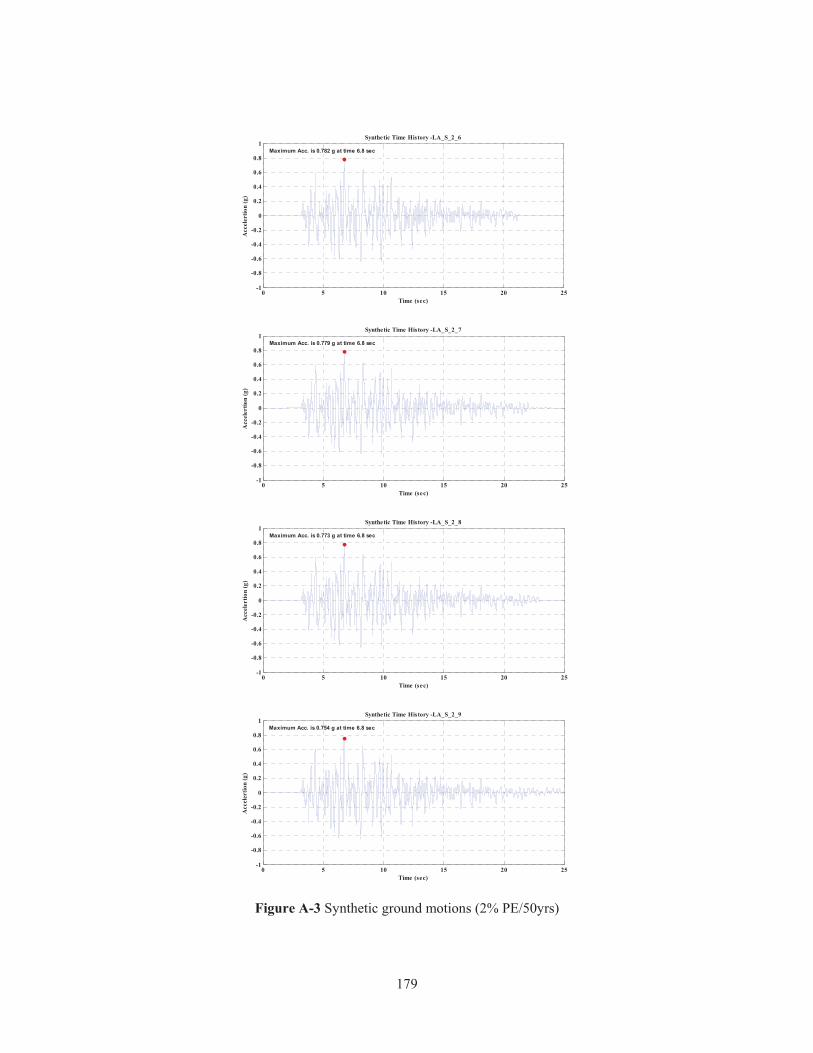
179
Figure A-3 Synthetic ground motions (2% PE/50yrs)
0 5 10 15 20 25-1
-0.8
-0.6
-0.4
-0.2
0
0.2
0.4
0.6
0.8
1
Time (sec)
Acc
eler
tion
(g)
Synthetic Time History -LA_S_2_6
Maximum Acc. is 0.782 g at time 6.8 sec
0 5 10 15 20 25-1
-0.8
-0.6
-0.4
-0.2
0
0.2
0.4
0.6
0.8
1
Time (sec)
Acc
eler
tion
(g)
Synthetic Time History -LA_S_2_7
Maximum Acc. is 0.779 g at time 6.8 sec
0 5 10 15 20 25-1
-0.8
-0.6
-0.4
-0.2
0
0.2
0.4
0.6
0.8
1
Time (sec)
Acc
eler
tion
(g)
Synthetic Time History -LA_S_2_8
Maximum Acc. is 0.773 g at time 6.8 sec
0 5 10 15 20 25-1
-0.8
-0.6
-0.4
-0.2
0
0.2
0.4
0.6
0.8
1
Time (sec)
Acc
eler
tion
(g)
Synthetic Time History -LA_S_2_9
Maximum Acc. is 0.754 g at time 6.8 sec

180
(a) Response spectrum
(b) Synthetic ground motion
Figure A-4 Response spectrum and synthetic ground motion for 5% PE/50 yrs hazard level
10-1
100
101
0
0.5
1
1.5
2
2.5
3Synthetic Ground Motions (5%PE/50yrs)
Period (sec)
Spec
tral
Acc
lera
tion
(g)
CB-NGA (median)median+epsilon*std.Syn. GMs.(Bedrock)-avgSyn. GMs. (Surface)-avg.Synthetic Records
0 5 10 15 20 25-1
-0.8
-0.6
-0.4
-0.2
0
0.2
0.4
0.6
0.8
1
Time (sec)
Acc
eler
tion
(g)
Synthetic Time History -LA_S_5_5
Maximum Acc. is 0.634 g at time 7.9 sec
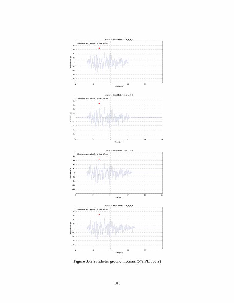
181
Figure A-5 Synthetic ground motions (5% PE/50yrs)
0 5 10 15 20 25-1
-0.8
-0.6
-0.4
-0.2
0
0.2
0.4
0.6
0.8
1
Time (sec)
Acc
eler
tion
(g)
Synthetic Time History -LA_S_5_1
Maximum Acc. is 0.667 g at time 6.7 sec
0 5 10 15 20 25-1
-0.8
-0.6
-0.4
-0.2
0
0.2
0.4
0.6
0.8
1
Time (sec)
Acc
eler
tion
(g)
Synthetic Time History -LA_S_5_2
Maximum Acc. is 0.668 g at time 6.7 sec
0 5 10 15 20 25-1
-0.8
-0.6
-0.4
-0.2
0
0.2
0.4
0.6
0.8
1
Time (sec)
Acc
eler
tion
(g)
Synthetic Time History -LA_S_5_3
Maximum Acc. is 0.666 g at time 6.7 sec
0 5 10 15 20 25-1
-0.8
-0.6
-0.4
-0.2
0
0.2
0.4
0.6
0.8
1
Time (sec)
Acc
eler
tion
(g)
Synthetic Time History -LA_S_5_4
Maximum Acc. is 0.667 g at time 6.7 sec

182
Figure A-5 Synthetic ground motions (5% PE/50yrs)
0 5 10 15 20 25-1
-0.8
-0.6
-0.4
-0.2
0
0.2
0.4
0.6
0.8
1
Time (sec)
Acc
eler
tion
(g)
Synthetic Time History -LA_S_5_6
Maximum Acc. is 0.633 g at time 7.9 sec
0 5 10 15 20 25-1
-0.8
-0.6
-0.4
-0.2
0
0.2
0.4
0.6
0.8
1
Time (sec)
Acc
eler
tion
(g)
Synthetic Time History -LA_S_5_7
Maximum Acc. is 0.633 g at time 7.9 sec
0 5 10 15 20 25-1
-0.8
-0.6
-0.4
-0.2
0
0.2
0.4
0.6
0.8
1
Time (sec)
Acc
eler
tion
(g)
Synthetic Time History -LA_S_5_8
Maximum Acc. is 0.633 g at time 7.9 sec
0 5 10 15 20 25-1
-0.8
-0.6
-0.4
-0.2
0
0.2
0.4
0.6
0.8
1
Time (sec)
Acc
eler
tion
(g)
Synthetic Time History -LA_S_5_9
Maximum Acc. is 0.633 g at time 7.9 sec

183
(a) Response spectrum
(b) Synthetic ground motion
Figure A-6 Response spectrum and synthetic ground motion for 10% PE/50 yrs hazard level
10-1
100
101
0
0.5
1
1.5
2
2.5
3Synthetic Ground Motions (10%PE/50yrs)
Period (sec)
Spec
tral
Acc
lera
tion
(g)
CB-NGA (median)median+epsilon*std.Syn. GMs.(Bedrock)-avgSyn. GMs. (Surface)-avg.Synthetic Records
0 5 10 15 20 25-1
-0.8
-0.6
-0.4
-0.2
0
0.2
0.4
0.6
0.8
1
Time (sec)
Acc
eler
tion
(g)
Synthetic Time History -LA_S_10_5
Maximum Acc. is 0.614 g at time 7.9 sec
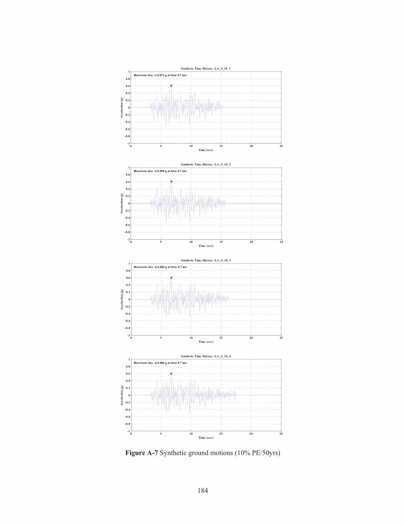
184
Figure A-7 Synthetic ground motions (10% PE/50yrs)
0 5 10 15 20 25-1
-0.8
-0.6
-0.4
-0.2
0
0.2
0.4
0.6
0.8
1
Time (sec)
Acc
eler
tion
(g)
Synthetic Time History -LA_S_10_1
Maximum Acc. is 0.611 g at time 6.7 sec
0 5 10 15 20 25-1
-0.8
-0.6
-0.4
-0.2
0
0.2
0.4
0.6
0.8
1
Time (sec)
Acc
eler
tion
(g)
Synthetic Time History -LA_S_10_2
Maximum Acc. is 0.609 g at time 6.7 sec
0 5 10 15 20 25-1
-0.8
-0.6
-0.4
-0.2
0
0.2
0.4
0.6
0.8
1
Time (sec)
Acc
eler
tion
(g)
Synthetic Time History -LA_S_10_3
Maximum Acc. is 0.608 g at time 6.7 sec
0 5 10 15 20 25-1
-0.8
-0.6
-0.4
-0.2
0
0.2
0.4
0.6
0.8
1
Time (sec)
Acc
eler
tion
(g)
Synthetic Time History -LA_S_10_4
Maximum Acc. is 0.606 g at time 6.7 sec

185
Figure A-7 Synthetic ground motions (10% PE/50yrs)
0 5 10 15 20 25-1
-0.8
-0.6
-0.4
-0.2
0
0.2
0.4
0.6
0.8
1
Time (sec)
Acc
eler
tion
(g)
Synthetic Time History -LA_S_10_6
Maximum Acc. is 0.614 g at time 7.9 sec
0 5 10 15 20 25-1
-0.8
-0.6
-0.4
-0.2
0
0.2
0.4
0.6
0.8
1
Time (sec)
Acc
eler
tion
(g)
Synthetic Time History -LA_S_10_7
Maximum Acc. is 0.614 g at time 7.9 sec
0 5 10 15 20 25-1
-0.8
-0.6
-0.4
-0.2
0
0.2
0.4
0.6
0.8
1
Time (sec)
Acc
eler
tion
(g)
Synthetic Time History -LA_S_10_8
Maximum Acc. is 0.615 g at time 7.9 sec
0 5 10 15 20 25-1
-0.8
-0.6
-0.4
-0.2
0
0.2
0.4
0.6
0.8
1
Time (sec)
Acc
eler
tion
(g)
Synthetic Time History -LA_S_10_9
Maximum Acc. is 0.615 g at time 7.9 sec

186
APPENDIX B
HYBRID SIMULATION TESTING DATA
In this section, instrumented data collected during the hybrid simulation testing
were included in the following pages. Tests were grouped in the following categories:
� Proof test
(Ground motion: the 1994 Northridge earthquake record)
� Mean PGA value for immediate occupancy limit state
(Ground motion: 10% probability of exceedance in 50 years)
� Mean PGA value for life safety limit state
(Ground motion: 5% probability of exceedance in 50 years)
� Mean PGA value for collapse prevention limit state
(Ground motion: 2% probability of exceedance in 50 years)
Meanwhile, multiplatform simulation testing was also conducted. Comparison
between hybrid and multiplatform simulation were made. Included for each testing are
the following:
� Testing description
� Applied ground motion
� Comparison of interstory drift angle (ISDA) between the target and the
one calculated based on hybrid simulation result.

187
� Relationship between lateral force and displacement on top of specimen
column.
� Displacement (lateral displacement, axial displacement and rotation)
history on the top of specimen column.
� Force (lateral force, axial force and moment) history on the top of
specimen column.
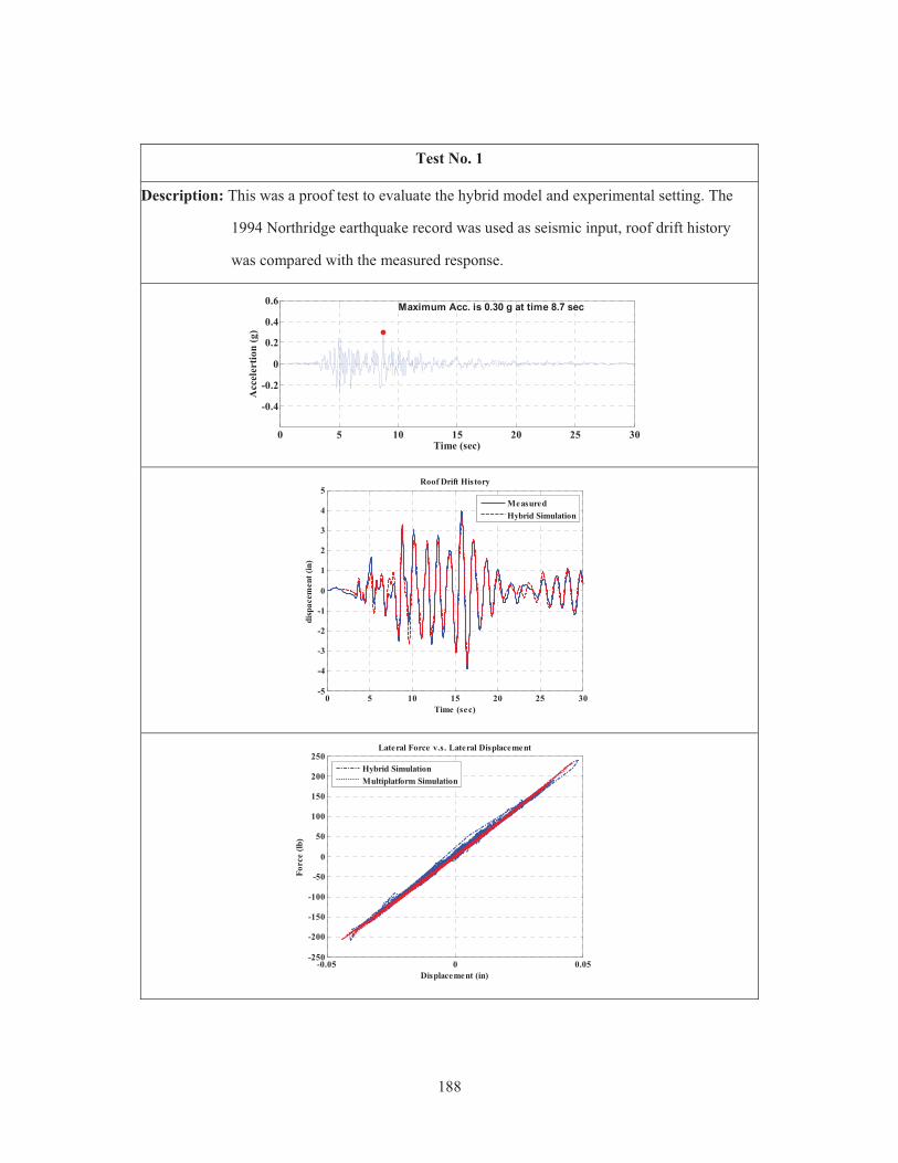
188
Test No. 1
Description: This was a proof test to evaluate the hybrid model and experimental setting. The
1994 Northridge earthquake record was used as seismic input, roof drift history
was compared with the measured response.
0 5 10 15 20 25 30
-0.4
-0.2
0
0.2
0.4
0.6
Time (sec)
Acc
eler
tion
(g)
Maximum Acc. is 0.30 g at time 8.7 sec
0 5 10 15 20 25 30-5
-4
-3
-2
-1
0
1
2
3
4
5Roof Drift History
Time (sec)
disp
acem
ent (
in)
MeasuredHybrid Simulation
-0.05 0 0.05-250
-200
-150
-100
-50
0
50
100
150
200
250Lateral Force v.s. Lateral Displacement
Displacement (in)
Forc
e (lb
)
Hybrid SimulationMultiplatform Simulation
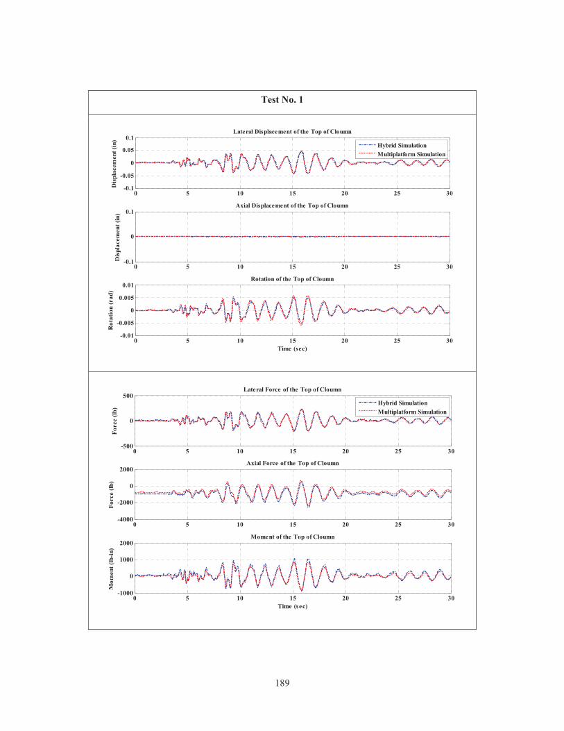
189
Test No. 1
0 5 10 15 20 25 30-0.1
-0.05
0
0.05
0.1Lateral Displacement of the Top of Cloumn
Disp
lace
men
t (in
)
Hybrid SimulationMultiplatform Simulation
0 5 10 15 20 25 30-0.1
0
0.1Axial Displacement of the Top of Cloumn
Disp
lace
men
t (in
)
0 5 10 15 20 25 30-0.01
-0.005
0
0.005
0.01Rotation of the Top of Cloumn
Time (sec)
Rot
atio
n (r
ad)
0 5 10 15 20 25 30-500
0
500Lateral Force of the Top of Cloumn
Forc
e (lb
)
Hybrid SimulationMultiplatform Simulation
0 5 10 15 20 25 30-4000
-2000
0
2000Axial Force of the Top of Cloumn
Forc
e (lb
)
0 5 10 15 20 25 30-1000
0
1000
2000Moment of the Top of Cloumn
Time (sec)
Mom
ent (
lb-in
)

190
Test No. 2
Description: This was the first test conducted to derive the mean PGA value for the immediate
occupancy limit state. 10% PE/50 yrs ground motion was selected as seismic input.
0 5 10 15 20 25 30-1
-0.5
0
0.5
1
Time (sec)
Acc
eler
tion
(g)
Maximum Acc. is 0.614 g at time 7.9 sec
0 1 2 3 4 5
0.007
0.025
0.05
ISDA = 0.008Scale factor for next testing = 0.89
ISDA(IO)
ISDA(LS)
ISDA(CP)
Number of Hybrid Simulation
Inte
rsto
ry D
rift
Ang
le (I
SDA
)
Immediate OccupancyLife SafetyCollapse Prevention
-0.1 -0.08 -0.06 -0.04 -0.02 0 0.02 0.04 0.06 0.08-400
-300
-200
-100
0
100
200
300
400Lateral Force v.s. Lateral Displacement
Displacement (in)
Forc
e (lb
)
Hybrid SimulationMultiplatform Simulation

191
Test No. 2
0 5 10 15 20 25-0.1
0
0.1Lateral Displacement of the Top of Cloumn
Dis
plac
emen
t (in
)Hybrid SimulationMultiplatform Simulation
0 5 10 15 20 25-0.1
0
0.1Axial Displacement of the Top of Cloumn
Dis
plac
emen
t (in
)
0 5 10 15 20 25-0.01
0
0.01
0.02Rotation of the Top of Cloumn
Time (sec)
Rot
atio
n (r
ad)
0 5 10 15 20 25-500
0
500Lateral Force of the Top of Cloumn
Forc
e (lb
)
Hybrid SimulationMultiplatform Simulation
0 5 10 15 20 25-4000
-2000
0
2000Axial Force of the Top of Cloumn
Forc
e (lb
)
0 5 10 15 20 25-2000
0
2000
4000Moment of the Top of Cloumn
Time (sec)
Mom
ent (
lb-in
)

192
Test No. 3
Description: This was the second test conducted to derive the mean PGA value for the
immediate occupancy limit state. 10% PE/50 yrs ground motion with scale factor
equal to 0.89 was selected as seismic input.
0 5 10 15 20 25 30-1
-0.5
0
0.5
1
Time (sec)
Acc
eler
tion
(g)
Maximum Acc. is 0.545 g at time 7.9 sec
0 1 2 3 4 5
0.007
0.025
0.05
ISDA = 0.0069 (Difference = 1.4%)
Mean PGA for IO limit state = 0.545 gISDA(IO)
ISDA(LS)
ISDA(CP)
Number of Hybrid Simulation
Inte
rsto
ry D
rift
Ang
le (I
SDA
)
Immediate OccupancyLife SafetyCollapse Prevention
-0.08 -0.06 -0.04 -0.02 0 0.02 0.04 0.06 0.08-400
-300
-200
-100
0
100
200
300
400Lateral Force v.s. Lateral Displacement
Displacement (in)
Forc
e (lb
)
Hybrid SimulationMultiplatform Simulation

193
Test No. 3
0 5 10 15 20 25-0.1
0
0.1Lateral Displacement of the Top of Cloumn
Dis
plac
emen
t (in
)Hybrid SimulationMultiplatform Simulation
0 5 10 15 20 25-0.1
0
0.1Axial Displacement of the Top of Cloumn
Dis
plac
emen
t (in
)
0 5 10 15 20 25-0.01
0
0.01Rotation of the Top of Cloumn
Time (sec)
Rot
atio
n (r
ad)
0 5 10 15 20 25-500
0
500Lateral Force of the Top of Cloumn
Forc
e (lb
)
Hybrid SimulationMultiplatform Simulation
0 5 10 15 20 25-4000
-2000
0
2000Axial Force of the Top of Cloumn
Forc
e (lb
)
0 5 10 15 20 25-2000
0
2000Moment of the Top of Cloumn
Time (sec)
Mom
ent (
lb-in
)

194
Test No. 4
Description: This was the first test conducted to derive the mean PGA value for the life safety
limit state. 5% PE/50 yrs ground motion was selected as seismic input.
0 5 10 15 20 25 30-1
-0.5
0
0.5
1
Time (sec)
Acc
eler
tion
(g)
Maximum Acc. is 0.634 g at time 7.9 sec
0 1 2 3 4 5
0.007
0.025
0.05
ISDA = 0.0098
Scale factor for next testing = 2.57ISDA(IO)
ISDA(LS)
ISDA(CP)
Number of Hybrid Simulation
Inte
rsto
ry D
rift
Ang
le (I
SDA
)
Immediate OccupancyLife SafetyCollapse Prevention
-0.15 -0.1 -0.05 0 0.05 0.1 0.15-500
-400
-300
-200
-100
0
100
200
300
400
500Lateral Force v.s. Lateral Displacement
Displacement (in)
Forc
e (lb
)
Hybrid SimulationMultiplatform Simulation

195
Test No. 4
0 5 10 15 20 25-0.2
-0.1
0
0.1
0.2Lateral Displacement of the Top of Cloumn
Dis
plac
emen
t (in
)Hybrid SimulationMultiplatform Simulation
0 5 10 15 20 25-0.2
-0.1
0
0.1
0.2Axial Displacement of the Top of Cloumn
Dis
plac
emen
t (in
)
0 5 10 15 20 25-0.02
-0.01
0
0.01
0.02Rotation of the Top of Cloumn
Time (sec)
Rot
atio
n (r
ad)
0 5 10 15 20 25-500
0
500Lateral Force of the Top of Cloumn
Forc
e (lb
)
Hybrid SimulationMultiplatform Simulation
0 5 10 15 20 25-4000
-2000
0
2000Axial Force of the Top of Cloumn
Forc
e (lb
)
0 5 10 15 20 25-2000
0
2000
4000Moment of the Top of Cloumn
Time (sec)
Mom
ent (
lb-in
)

196
Test No. 5
Description: This was the second test conducted to derive the mean PGA value for the life safety
limit state. 5% PE/50 yrs ground motion with scale factor equal to 2.57 was
selected as seismic input.
0 5 10 15 20 25 30-2
-1
0
1
2
Time (sec)
Acc
eler
tion
(g)
Maximum Acc. is 1.627 g at time 7.9 sec
0 1 2 3 4 5
0.007
0.025
0.05
ISDA = 0.0247 (Difference = 1.2%)
Mean PGA for LS limit state = 1.627 g
ISDA(IO)
ISDA(LS)
ISDA(CP)
Number of Hybrid Simulation
Inte
rsto
ry D
rift
Ang
le (I
SDA
)
Immediate OccupancyLife SafetyCollapse Prevention
-0.15 -0.1 -0.05 0 0.05 0.1 0.15 0.2 0.25 0.3-800
-600
-400
-200
0
200
400
600
800
1000Lateral Force v.s. Lateral Displacement
Displacement (in)
Forc
e (lb
)
Hybrid SimulationMultiplatform Simulation
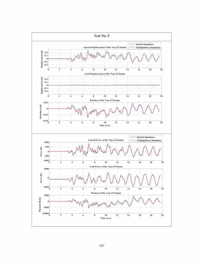
197
Test No. 5
0 2 4 6 8 10 12 14 16 18 20
-0.2-0.1
00.10.2
Lateral Displacement of the Top of Cloumn
Dis
plac
emen
t (in
)Hybrid SimulationMultiplatform Simulation
0 2 4 6 8 10 12 14 16 18 20
-0.2-0.1
00.10.2
Axial Displacement of the Top of Cloumn
Dis
plac
emen
t (in
)
0 2 4 6 8 10 12 14 16 18 20-0.04
-0.02
0
0.02Rotation of the Top of Cloumn
Time (sec)
Rot
atio
n (r
ad)
0 2 4 6 8 10 12 14 16 18 20-1000
-500
0
500
1000Lateral Force of the Top of Cloumn
Forc
e (lb
)
Hybrid SimulationMultiplatform Simulation
0 2 4 6 8 10 12 14 16 18 20-5000
0
5000Axial Force of the Top of Cloumn
Forc
e (lb
)
0 2 4 6 8 10 12 14 16 18 20-10000
-5000
0
5000Moment of the Top of Cloumn
Time (sec)
Mom
ent (
lb-in
)

198
Test No. 6
Description: This was the first test conducted to derive the mean PGA value for the collapse
prevention limit state. 2% PE/50 yrs ground motion was selected as seismic input.
0 5 10 15 20 25 30-2
-1
0
1
2
Time (sec)
Acc
eler
tion
(g)
Maximum Acc. is 0.784 g at time 6.8 sec
0 1 2 3 4 5
0.007
0.025
0.05
ISDA = 0.0156
Scale factor for next testing = 3.2
ISDA(IO)
ISDA(LS)
ISDA(CP)
Number of Hybrid Simulation
Inte
rsto
ry D
rift
Ang
le (I
SDA
)
Immediate OccupancyLife SafetyCollapse Prevention
-0.2 -0.15 -0.1 -0.05 0 0.05 0.1 0.15-600
-400
-200
0
200
400
600Lateral Force v.s. Lateral Displacement
Displacement (in)
Forc
e (lb
)
Hybrid SimulationMultiplatform Simulation

199
Test No. 6
0 5 10 15 20 25-0.2
-0.1
0
0.1
0.2Lateral Displacement of the Top of Cloumn
Dis
plac
emen
t (in
)
Hybrid SimulationMultiplatform Simulation
0 5 10 15 20 25-0.2
-0.1
0
0.1
0.2Axial Displacement of the Top of Cloumn
Dis
plac
emen
t (in
)
0 5 10 15 20 25-0.02
-0.01
0
0.01
0.02Rotation of the Top of Cloumn
Time (sec)
Rot
atio
n (r
ad)
0 5 10 15 20 25-1000
0
1000Lateral Force of the Top of Cloumn
Forc
e (lb
)
Hybrid SimulationMultiplatform Simulation
0 5 10 15 20 25-5000
0
5000Axial Force of the Top of Cloumn
Forc
e (lb
)
0 5 10 15 20 25-5000
0
5000Moment of the Top of Cloumn
Time (sec)
Mom
ent (
lb-in
)

200
Test No. 7
Description: This was the second test conducted to derive the mean PGA value for the collapse
prevention limit state. 2% PE/50 yrs ground motion with scale factor equal to 3.2
was selected as seismic input.
0 5 10 15 20 25 30-3
-2
-1
0
1
2
3
Time (sec)
Acc
eler
tion
(g)
Maximum Acc. is 2.507 g at time 6.8 sec
0 1 2 3 4 5
0.007
0.025
0.05ISDA = 0.043
Scale factor for next testing = 3.54
ISDA(IO)
ISDA(LS)
ISDA(CP)
Number of Hybrid Simulation
Inte
rsto
ry D
rift
Ang
le (I
SDA
)
Immediate OccupancyLife SafetyCollapse Prevention
-0.3 -0.2 -0.1 0 0.1 0.2 0.3 0.4 0.5-1000
-500
0
500
1000
1500Lateral Force v.s. Lateral Displacement
Displacement (in)
Forc
e (lb
)
Hybrid SimulationMultiplatform Simulation

201
Test No. 7
0 5 10 15 20 25-0.5
0
0.5Lateral Displacement of the Top of Cloumn
Dis
plac
emen
t (in
)
Hybrid SimulationMultiplatform Simulation
0 5 10 15 20 25-0.5
0
0.5Axial Displacement of the Top of Cloumn
Dis
plac
emen
t (in
)
0 5 10 15 20 25-0.1
0
0.1Rotation of the Top of Cloumn
Time (sec)
Rot
atio
n (r
ad)
0 5 10 15 20 25-1000
0
1000
2000Lateral Force of the Top of Cloumn
Forc
e (lb
) Hybrid SimulationMultiplatform Simulation
0 5 10 15 20 25-5000
0
5000Axial Force of the Top of Cloumn
Forc
e (lb
)
0 5 10 15 20 25-1
0
1x 10
4 Moment of the Top of Cloumn
Time (sec)
Mom
ent (
lb-in
)

202
Test No. 8
Description: This was the third test conducted to derive the mean PGA value for the collapse
prevention limit state. 2% PE/50 yrs ground motion with scale factor equal to 3.54
was selected as seismic input.
0 5 10 15 20 25 30-3
-2
-1
0
1
2
3
Time (sec)
Acc
eler
tion
(g)
Maximum Acc. is 2.777 g at time 6.8 sec
0 1 2 3 4 5
0.007
0.025
0.05
ISDA = 0.0495 (Difference = 1%)
Mean PGA for CP limit state = 2.777 g
ISDA(IO)
ISDA(LS)
ISDA(CP)
Number of Hybrid Simulation
Inte
rsto
ry D
rift
Ang
le (I
SDA
)
Immediate OccupancyLife SafetyCollapse Prevention
-0.3 -0.2 -0.1 0 0.1 0.2 0.3 0.4 0.5 0.6-1000
-500
0
500
1000
1500Lateral Force v.s. Lateral Displacement
Displacement (in)
Forc
e (lb
)
Hybrid SimulationMultiplatform Simulation

203
Test No. 8
0 5 10 15 20 25-0.5
0
0.5Lateral Displacement of the Top of Cloumn
Dis
plac
emen
t (in
)
Hybrid SimulationMultiplatform Simulation
0 5 10 15 20 25-0.5
0
0.5Axial Displacement of the Top of Cloumn
Dis
plac
emen
t (in
)
0 5 10 15 20 25-0.1
0
0.1Rotation of the Top of Cloumn
Time (sec)
Rot
atio
n (r
ad)
0 5 10 15 20 25-1000
0
1000
2000Lateral Force of the Top of Cloumn
Forc
e (lb
) Hybrid SimulationMultiplatform Simulation
0 5 10 15 20 25-10000
-5000
0
5000Axial Force of the Top of Cloumn
Forc
e (lb
)
0 5 10 15 20 25-1
0
1x 10
4 Moment of the Top of Cloumn
Time (sec)
Mom
ent (
lb-in
)

204
APPENDIX C
FRAGILITY RELATIONSHIPS FOR OTHER BUILDING TYPES
In this section, procedures and results using Parameterized Fragility Method
(PFM, Jeong and Elnashai, 2006) to derive fragility relationships for 36 building types
under 4 code levels were presented.
C.1 Structural Parameters for PFM
Figure C-1 tabulates the structural parameters which were fed into PFM to derive
fragility relationships for 36 building types under 4 code levels. This table is based on the
HAZUS-MH Technical Manual but updated with the latest research findings in wood
frame (Gencturk and Elnashai, 2008) and unreinforced masonry building (Frankie, 2010).
C.2 Earthquake Demand
Synthetic ground motions generated for the Burbank site (Appendix A) were used
as earthquake demand in PFM.
C.3 Fragility Relationships
With the above structural parameters and earthquake demand, PFM was
performed. Eventually, fragility relationships for 36 building types under 4 code levels
were generated. Figure C-2 tabulated the fragility relationships results.

205
Figu
re C
-1 S
truct
ural
par
amet
ers f
or P
FM to
gen
erat
e fr
agili
ty re
latio
nshi
ps
Nam
eSt
orie
sH
igh-
Cod
eM
oder
ate-
Cod
eL
ow-C
ode
Pre-
Cod
e1
W1*
Woo
d, L
ight
Fra
me
( >=
5,00
0 sq
. ft.)
1-
20.
351.
150.
810.
470.
232
W2*
Woo
d, C
omm
erci
al a
nd In
dust
rial (
> 5
,000
sq. f
t.)
All
0.4
0.67
0.41
0.24
0.14
3S1
LLo
w-R
ise1-
30.
50.
749
0.37
50.
187
0.18
74
S1M
Mid
-Rise
4-7
1.08
0.46
80.
234
0.11
70.
117
5S1
HH
igh-
Rise
8+2.
210.
293
0.14
70.
073
0.07
36
S2L
Low
-Rise
1-3
0.4
0.8
0.4
0.2
0.2
7S2
MM
id-R
ise4-
70.
860.
667
0.33
30.
167
0.16
78
S2H
Hig
h-R
ise8+
1.77
0.50
80.
254
0.12
70.
127
9S3
Stee
l Lig
ht F
ram
e A
ll0.
40.
80.
40.
20.
210
S4L
Low
-Rise
1-3
0.35
0.72
0.36
0.18
0.18
11S4
MM
id-R
ise4-
70.
650.
60.
30.
150.
1512
S4H
Hig
h-R
ise8+
1.32
0.45
70.
228
0.11
40.
114
13S5
LLo
w-R
ise1-
30.
350.
20.
214
S5M
Mid
-Rise
4-7
0.65
0.16
70.
167
15S5
HH
igh-
Rise
8+1.
320.
127
0.12
716
C1L
Low
-Rise
1-3
0.4
0.74
90.
375
0.18
70.
187
17C
1MM
id-R
ise4-
70.
750.
624
0.31
20.
156
0.15
618
C1H
Hig
h-R
ise8+
1.45
0.29
30.
147
0.07
30.
073
19C
2LLo
w-R
ise1-
30.
351
0.5
0.25
0.25
20C
2MM
id-R
ise4-
70.
560.
833
0.41
70.
208
0.20
821
C2H
Hig
h-R
ise8+
1.09
0.63
50.
317
0.15
90.
159
22C
3LLo
w-R
ise1-
30.
350.
225
0.22
523
C3M
Mid
-Rise
4-7
0.56
0.18
80.
188
24C
3HH
igh-
Rise
8+1.
090.
143
0.14
325
PC1
Prec
ast C
oncr
ete
Tilt-
Up
Wal
lsA
ll0.
351.
20.
60.
30.
326
PC2L
Low
-Rise
1-3
0.35
0.8
0.4
0.2
0.2
27PC
2MM
id-R
ise4-
70.
560.
667
0.33
30.
167
0.16
728
PC2H
Hig
h-R
ise8+
1.09
0.50
80.
254
0.12
70.
127
29R
M1L
Low
-Rise
1-3
0.35
1.06
60.
533
0.26
70.
267
30R
M1M
Mid
-Rise
4+0.
560.
889
0.44
40.
222
0.22
231
RM
2LLo
w-R
ise1-
30.
351.
066
0.53
30.
267
0.26
732
RM
2MM
id-R
ise4-
70.
560.
889
0.44
40.
222
0.22
233
RM
2HH
igh-
Rise
8+1.
090.
677
0.33
80.
169
0.16
934
UR
ML
**Lo
w-R
ise1-
20.
350.
30.
335
UR
MM
**M
id-R
ise3+
0.5
0.22
20.
222
36M
HM
obile
Hom
es
All
0.35
0.3
0.3
0.3
0.3
No.
Lab
elD
escr
iptio
nH
eigh
tPe
riod
SR-U
ltim
ate
stre
ngth
Ran
ge
Stee
l Mom
ent F
ram
e
Stee
l Bra
ced
Fram
e
Stee
l Fra
me
with
Cas
t-in-
Plac
e Co
ncre
te S
hear
Wal
ls
Stee
l Fra
me
with
Unr
einf
orce
d M
ason
ry In
fill W
alls
Con
cret
e M
omen
t Fra
me
Con
cret
e Sh
ear W
alls
* G
enct
urk
and
Elna
shai
, 200
8**
Fra
nkie
, 201
0
Con
cret
e Fr
ame
with
Unr
einf
orce
d M
ason
ry In
fill W
alls
Prec
ast C
oncr
ete
Fram
es w
ith C
oncr
ete
Shea
r Wal
ls
Rei
nfor
ced
Mas
onry
Bea
ring
Wal
ls w
ith W
ood
or M
etal
Dec
k D
iaph
ragm
s
Rei
nfor
ced
Mas
onry
Bea
ring
Wal
ls w
ith P
reca
st C
oncr
ete
Dia
phra
gms
Unr
einf
orce
d M
ason
ry B
earin
g W
alls

206
Figu
re C
-2 F
ragi
lity
rela
tions
hips
dat
abas
e (P
FM a
long
with
hyb
rid fr
agili
ty a
ppro
ach)
��
��
��
��
��
��
��
��
��
��
��
��
W1
-1.2
590.
635
0.14
80.
618
1.30
20.
617
-1.4
250.
624
0.07
00.
613
0.99
10.
611
-1.3
670.
477
-0.0
250.
465
0.68
10.
522
-1.7
130.
490
-0.1
100.
486
0.29
20.
515
W2
-0.5
170.
421
0.19
30.
436
1.35
80.
494
-0.6
890.
422
0.12
50.
438
1.06
10.
492
-0.9
240.
344
0.01
50.
362
0.59
60.
403
-1.3
830.
341
-0.1
220.
351
0.10
10.
393
S1L
-0.6
780.
520
0.18
90.
541
0.99
70.
535
-0.8
040.
535
-0.0
290.
547
0.82
20.
562
-0.9
080.
496
-0.3
080.
504
0.35
70.
490
-1.2
040.
492
-0.6
330.
497
0.05
50.
495
S1M
*-0
.607
0.31
10.
487
0.32
81.
021
0.34
6-0
.744
0.47
3-0
.024
0.48
10.
792
0.48
9-0
.815
0.49
5-0
.139
0.49
80.
644
0.49
8-1
.087
0.50
4-0
.450
0.50
20.
256
0.49
4
S1H
-0.4
040.
473
0.42
40.
474
1.27
70.
473
-0.5
580.
470
0.16
10.
469
0.94
60.
467
-0.6
730.
463
-0.0
240.
468
0.76
70.
477
-0.9
090.
483
-0.2
800.
487
0.42
30.
481
S2L
-0.5
500.
553
0.61
10.
569
1.56
00.
555
-0.6
770.
547
0.33
60.
571
1.18
20.
559
-0.9
470.
471
-0.1
370.
486
0.61
50.
478
-1.3
450.
456
-0.6
590.
474
0.03
10.
466
S2M
-0.5
610.
492
0.50
70.
506
1.53
90.
534
-0.6
200.
523
0.40
40.
545
1.36
20.
551
-0.7
860.
486
0.01
90.
488
0.79
90.
488
-1.1
360.
483
-0.4
180.
477
0.27
60.
472
S2H
-0.5
150.
496
0.50
00.
518
1.37
00.
522
-0.6
440.
500
0.28
90.
522
1.14
90.
525
-0.6
880.
511
0.19
30.
527
0.98
10.
515
-0.9
720.
523
-0.1
390.
542
0.57
30.
525
S3-1
.411
0.49
0-0
.457
0.50
10.
445
0.49
2-1
.577
0.47
8-0
.732
0.48
70.
158
0.50
2-1
.663
0.49
4-0
.876
0.49
8-0
.102
0.47
8-1
.903
0.49
8-1
.157
0.49
6-0
.409
0.47
8
S4L
-0.4
770.
540
0.61
80.
540
1.50
60.
496
-0.6
550.
516
0.26
70.
527
1.11
10.
505
-0.8
550.
459
-0.0
760.
478
0.76
30.
475
-1.2
030.
465
-0.5
200.
463
0.18
70.
448
S4M
-0.4
330.
502
0.64
00.
511
1.70
60.
523
-0.4
220.
555
0.57
60.
554
1.59
00.
556
-0.6
470.
488
0.17
40.
493
1.04
30.
496
-1.0
350.
471
-0.3
190.
471
0.43
30.
463
S4H
-0.3
690.
472
0.64
10.
477
1.59
70.
480
-0.4
970.
477
0.42
40.
482
1.39
10.
491
-0.5
570.
490
0.29
40.
490
1.13
50.
481
-0.8
800.
484
-0.1
040.
482
0.66
80.
474
S5L
-0.9
510.
504
-0.1
170.
510
0.53
70.
492
-1.2
780.
500
-0.4
850.
517
0.18
70.
503
S5M
-0.6
890.
515
0.17
40.
520
0.83
80.
510
-1.0
190.
518
-0.2
170.
524
0.47
70.
523
S5H
-0.7
210.
459
0.00
30.
443
0.64
00.
438
-0.9
710.
471
-0.2
630.
456
0.33
80.
448
C1L
-0.5
760.
540
0.54
80.
547
1.51
60.
538
-0.6
930.
546
0.28
80.
566
1.15
20.
561
-0.8
830.
477
-0.0
670.
500
0.76
50.
509
-1.2
730.
465
-0.5
070.
491
0.17
80.
480
C1M
-0.4
830.
479
0.55
90.
495
1.54
40.
522
-0.4
790.
545
0.51
70.
552
1.46
70.
560
-0.6
870.
482
0.10
90.
487
0.90
80.
488
-1.0
510.
463
-0.3
300.
469
0.35
40.
465
C1H
-0.5
020.
476
0.50
40.
472
1.37
30.
475
-0.5
950.
502
0.37
30.
508
1.32
60.
522
-0.7
570.
472
-0.0
260.
459
0.58
70.
449
-1.0
410.
468
-0.3
510.
453
0.22
30.
440
C2L
-0.4
750.
530
0.62
10.
528
1.47
20.
489
-0.6
720.
511
0.27
50.
521
1.08
00.
506
-0.8
310.
490
-0.0
090.
495
0.75
50.
486
-1.1
720.
475
-0.4
380.
476
0.25
10.
466
C2M
-0.3
430.
505
0.75
20.
531
1.80
70.
552
-0.3
690.
554
0.65
90.
561
1.63
70.
573
-0.5
720.
505
0.32
50.
523
1.20
50.
520
-0.9
440.
490
-0.1
480.
511
0.61
10.
504
C2H
-0.4
040.
473
0.58
80.
472
1.41
70.
475
-0.5
530.
487
0.39
50.
497
1.30
30.
517
-0.6
010.
503
0.32
70.
514
1.23
60.
528
-0.9
250.
494
-0.1
150.
496
0.68
60.
511
C3L
-1.1
490.
488
-0.3
260.
505
0.33
50.
484
-1.4
580.
483
-0.6
770.
510
-0.0
070.
493
C3M
-0.8
450.
509
0.02
80.
527
0.76
40.
522
-1.1
560.
511
-0.3
380.
528
0.41
30.
536
C3H
-0.8
570.
510
-0.0
230.
514
0.63
80.
506
-1.1
530.
499
-0.3
850.
497
0.24
20.
488
PC1
-1.0
830.
501
-0.0
130.
508
0.97
60.
480
-1.1
830.
511
-0.2
650.
514
0.66
60.
501
-1.2
630.
499
-0.4
730.
505
0.35
50.
483
-1.5
940.
489
-0.8
680.
479
-0.1
190.
460
PC2L
-0.6
980.
537
0.39
70.
535
1.31
90.
494
-0.8
570.
516
0.06
70.
528
0.93
60.
506
-1.0
200.
471
-0.2
420.
485
0.60
80.
479
-1.3
630.
467
-0.6
560.
470
0.07
70.
457
PC2M
-0.5
210.
528
0.58
00.
539
1.68
60.
549
-0.5
630.
555
0.45
60.
565
1.51
20.
571
-0.7
570.
498
0.08
00.
508
0.98
70.
510
-1.1
180.
484
-0.3
930.
491
0.37
20.
488
PC2H
-0.6
260.
473
0.36
10.
472
1.27
00.
473
-0.7
180.
504
0.27
20.
525
1.33
50.
549
-0.7
610.
512
0.13
70.
520
1.08
60.
522
-1.1
110.
491
-0.3
010.
500
0.51
10.
497
RM
1L-0
.740
0.52
20.
358
0.52
51.
331
0.48
9-0
.875
0.51
10.
045
0.51
90.
947
0.50
4-1
.000
0.49
5-0
.208
0.49
80.
643
0.49
2-1
.340
0.48
8-0
.624
0.48
20.
141
0.46
5
RM1M
-0.5
970.
492
0.47
10.
521
1.60
90.
545
-0.6
050.
551
0.39
20.
555
1.44
40.
566
-0.7
570.
504
0.09
80.
521
1.06
30.
526
-1.0
940.
493
-0.3
390.
506
0.50
60.
513
RM
2L-0
.740
0.52
20.
358
0.52
51.
331
0.48
9-0
.875
0.51
10.
045
0.51
90.
947
0.50
4-1
.000
0.49
5-0
.208
0.49
80.
643
0.49
2-1
.340
0.48
8-0
.624
0.48
20.
141
0.46
5
RM2M
-0.5
970.
492
0.47
10.
521
1.60
90.
545
-0.6
050.
551
0.39
20.
555
1.44
40.
566
-0.7
570.
504
0.09
80.
521
1.06
30.
526
-1.0
940.
493
-0.3
390.
506
0.50
60.
513
RM2H
-0.6
260.
473
0.36
50.
472
1.28
50.
475
-0.7
550.
483
0.15
10.
489
1.11
20.
506
-0.7
930.
501
0.09
80.
514
1.08
40.
528
-1.0
930.
498
-0.3
040.
500
0.56
20.
511
URM
L-1
.441
0.45
4-0
.678
0.46
1-0
.036
0.43
5-1
.683
0.46
3-0
.971
0.45
9-0
.339
0.44
1
URM
M-1
.201
0.50
0-0
.538
0.52
60.
105
0.52
1-1
.479
0.51
1-1
.020
0.52
2-0
.346
0.52
8
MH
-1.5
160.
570
-0.4
280.
571
0.50
30.
518
-1.5
160.
570
-0.4
280.
571
0.50
30.
518
-1.5
160.
570
-0.4
280.
571
0.50
30.
518
-1.8
640.
546
-0.8
620.
542
0.07
50.
529
Low
-Cod
e Sei
smic
Des
ign
Leve
l
IOL
SC
P
Pre-
Cod
e Se
ism
ic D
esig
n L
evel
PGA
(g)
PG
A (g
)
Hig
h-C
ode
Seis
mic
Des
ign
Lev
elM
oder
ate-
Cod
e Se
ism
ic D
esig
n L
evel
IOL
SC
PPG
A (g
)IO
LS
CP
*Hyb
rid
fragi
lity a
ppro
ach
Build
ing
Typ
esIO
LS
CP
PGA
(g)

207
APPENDIX D
AN EFFICIENT MODEL CALIBRATION METHOD
An automatic system identification-based model updating technique was
developed and incorporated into NISRAF. Provided below, the methodology, procedures
and GUIs of this method are developed by Jian Li at University of Illinois (Li et al.,
2009).
D.1 System Identification
Among the state-space based system identification methods, Eigensystem
Realization Algorithm (ERA) (Juang and Pappa, 1985) is selected to identify the modal
parameters of structures, due to its wide application and good performance in multi-input
multi-output (MIMO) problems. The basic idea of ERA is to find a minimum realization
of system (state-space representation with minimum dimension) using Singular Value
Decomposition (SVD) on the Hankel matrix built by Markov parameters (impulse
response functions). The modal properties can be extracted from the realized minimum
state-space representation. Therefore, to start with ERA, ‘generalized Hankel matrices’
are constructed, assuming that there are p inputs and q outputs:
ÄÅ�* , � Æ Ç* , È Ç* � k + �,É Ê ÉÇ* � � + �, È Ç* � � � k + �,Ë (D.1)

208
where k = 0, 1; Ç* , is the impulse response function at time k, consisting of p rows and
q columns; r and s are the number of block rows and block columns. Singular value
decomposition is then performed for ÄÅ�* , which yields:
ÄÅ�*�, � Ì Í ÎÏ (D.2)
where Ì and Î are unitary matrices, Í is an r×p by s×q diagonal matrix with singular
values on the diagonal. The number of non-zero singular values gives the dimension of
the minimum realization of the system if Ç* , is noise free. In reality this is not the case,
therefore Í is usually of full rank. The singular values corresponding to noise are usually
much smaller compared with those corresponding to real modes. By preserving the first
N ordered significant singular values, by which noise modes are eliminated, the minimum
realization can be calculated as follows:
Ð � Íd% )� ÌDÄÅ�*�,ÎÍd% )�Ñ � Í% )� ÎÒÓÔ � ÒÕDÌÍ% )� (D.3)
In the above equations, Ì and Î contain the first N corresponding columns of Ì and Î,
respectively. ÒÕD � `ÖÕ �Õ!!!!!× �Õa and ÒÓD � `ÖÓ �Ó!!!!!× �Óa . The realization is
then transformed to modal coordinates by using the eigenvalues Z and eigenvector matrix
of A, which yields:

209
ÐØ � Ùd�ÐÙ � ÚÑ � Ùd�ÑÔ � ÔÙ (D.4)
Modal participation factors and mode shapes are the corresponding rows of ÑØ and
columns of ÔØ, respectively. The modal damping ratio ÛÜ and damped natural frequencies
�� can be calculated from the eigenvalues of A after transforming back to continuous
domain:
k� � +Þ�ß�� � oß�� � 34*à�, Xáâ (D.5)
where ß�� � ß��X5� + Þ�) are undamped natural frequencies, and ãâ is the sampling
interval.
A two-step strategy is applied to filter out computational and noise modes. Since
more singular values are retained, more potential genuine modes can be identified. In this
study, the dimension of realized system N is increased in a range until adequate modes
are included finally. First, for each particular order of system, three commonly used mode
accuracy indicators, namely Modal Amplitude Coherence (MAC) (Juang and Pappa,
1985), Extended Modal Amplitude Coherence (EMAC) and Modal Phase Colinearity
(MPC) (Pappa and Elliott, 1993) are used to filter out the computational or noise modes.
The retained modes are then deemed trustable and a stabilization diagram is plotted for
further confirmation. The stabilization diagram gathers all modes identified from the
realized systems with different system order, based on the idea that a genuine mode
should always be identified with a different order of realized system, as long as the

210
system order is adequate for that mode. Among the same order of modes identified and
plotted in the stabilization diagram, the one with highest EMAC value is then selected as
the final confirmed mode.
D.2 Model Updating
For model updating, to keep the physical meaning, the iterative or parametric
method is implemented in NISRAF. Currently, only linear model updating is available. In
the linear approach, the objective function represented the modal parameter (natural
frequencies and mode shapes) residuals are formed as linear combination of natural
frequency residuals and model shape residuals with different weighting factors.
<*ä, � À� £R��½ + � ½� ½ S)Aå
½±% � À� £æçèd%²«&^¯½³*é �� ,Aê½±%
(D.6)
where ��½ and � ½ denote analytical and experimental natural frequencies; À� and À� are
weighting factor applied to frequency residuals and mode shape residuals, respectively.
0.8 and 0.2 are used here considering the factor that natural frequencies usually have
higher accuracy than mode shapes in practical system identification. MAC (Modal
Assurance Criteria) is a measurement of mode shape discrepancy and is defined as
Equation (D.7) (Allemang and Brown, 1982).
&^ � � *ë��D ë �,)*ë��D ë��,*ë �D ë �, (D.7)

211
where ë�� and ë � are analytical and experimental mode shapes. MAC = 1 means ë�� and
ë � are perfectly matched and MAC = 0 means they are orthogonal. It is known that MAC
is rather insensitive to the change of mode shape. Also it is noticed that MAC is actually
the square of the inner product between the two mode shape vectors. Therefore, the
objective function for mode shape residual is formed as the normalized angle between the
two mode shape vectors, which is much more sensitive to the change of mode shape.
Nelder-Mead method (Nelder and Mead, 1965) is applied to solve the
optimization problem defined above. This method is computationally quite simple and
relatively robust. It requires no computation of derivative information; iteration is driven
by the evaluation of the value of objective function only. The algorithm starts by
generating a set of 1n vertices that defines a simplex, where n is the number of
parameters to be updated. Then a set of tie-breaking rules, including reflection, expansion,
contraction and shrinkage, are carried out to update the simplex for the next iteration until
convergence rules are satisfied.