An Analysis on Airport-Airline Vertical Relationships with ...

GraSPP-DP-E-11-001 and ITPU-DP-E-11-001

An Analysis on Airport-Airline Vertical

Relationships with Risk Sharing Contracts under Asymmetric Information Structures

Katsuya Hihara

June 2011

GraSPP Discussion Paper E-11-001 ITPU Discussion Paper E-11-001

GraSPP-DP-E-11-001 and ITPU-DP-E-11-001

An Analysis on Airport-Airline Vertical

Relationships with Risk Sharing Contracts under Asymmetric Information Structures

Katsuya Hihara

June 2011

Professor, Graduate School of Public PolicyThe University of Tokyo

7-3-1, Hongo, Bunkyo-ku, Tokyo, 113-0033, JapanPhone: +81-3-5841-1710

Fax: [email protected]

GraSPP Discussion Papers can be downloaded without charge from: http://www.pp.u-tokyo.ac.jp/

Discussion Papers are a series of manuscripts in their draft form. They are not intended for circulation or distribution except as indicated by the author. For that reason

Discussion Papers may not be reproduced or distributed without the written consent of the author.

An Analysis on Airport-Airline VerticalRelationships with Risk Sharing Contracts under

Asymmetric Information Structures

Katsuya Hihara∗

2011/06/10 1830 JST

Abstract

We analyze the double moral hazard problem at the joint venture typeairport-airline vertical relationship, where two parties both contribute effortsto the joint venture but neither of them can see the other’s efforts. Withthe continuous-time stochastic dynamic programming model, we show thatby the de-centralized utility maximizations of two parties under very strictconditions, i.e., optimal efforts’ cost being negligible and their risk averseparameters both asymptotically approaching to zero, the vertical contract,which is linear function of the final state with the slope being the productmade by their productivity difference and uncertainty (diffusion rate) levelindex, could be agreed as the optimal sharing rule.

If both parties’productivities are same, or the diffusion rate of the under-lying process is unity, optimal linear sharing rule do not depend on the finalstate. If their conditions not dependent on final state are symmetric as well,then risk sharing disappears completely. In numerical examples, we illustratethe complex impact of uncertainty increase and end-of-period load factor im-provement on the optimal sharing rule, and the relatively simple impact ontotal utilities level.

Key wordsAirport-Airline Vertical Relationship, Load Factor Guarantee Mechanism, DoubleHidden Action/Moral Hazard, Risk Sharing, Stochastic Dynamic Programming

JEL Classification Numbers:C61,C73,D82,D86,L14,L93

∗Corresponding author; Tel:+81-3-5841-1710, Fax:+81-3-5841-7877, E-mail address:[email protected], GraSPP, University of Tokyo, 7-3-1 Hongo Bunkyo-ku Tokyo, JapanPreliminary Draft. Do not quote without written permission of the author.

1

1 Introduction

Faced with revenue and profit level fluctuations, some airports (local governments)and airlines serving the airports are forming vertical contractual relationship toshare their risk and stabilize their financial conditions so that air transport servicesby those airlines to/from the airports could be created or kept.

Hihara (2008) and Hihara (2010) reports that Noto Airport, one of rural airports inJapan, agreed on contract with one airline group to share the demand fluctuationrisk so as to derive the commitment of airline’s service to the airport. They usedload factor as a key indicator. So the mechanism of the contract is called load factorguarantee mechanism. Also Hihara (2010) analyzed by using incomplete contractframework to show that when such vertical risk sharing contract satisfy properconditions, such contract can overcome the under-effort problem and improve theutilities levels of both parties.

2 Past Literature

Risk sharing study dates back to Borch (1962). He showed that under pure risksharing situation without any efforts, the optimal sharing rule stipulates that theratio of marginal utility of two participating parties in different state are constantand the results hold for any probability distribution.

The risk sharing is also the subject of moral hazard analysis, since the principalis paying to the agent based on the realization of uncertain state. The essence ofrisk sharing is to share the outcome depend on the realization of contingencies bypaying from one party to the other(s) based on some rule. The moral hazard case,the effort of the agent is involved and the principal is optimizing his utilities bycontrolling payment and also agent’s efforts indirectly through the payment struc-ture.

There are two approaches to model the uncertainty in the moral hazard situation.First is that random variable with some probability distribution is assigned to thestate itself. This approach dates back to Mirrlees( for example, Mirrlees (1979))and Rogerson (1985) prove that under this settings, the first order approach is per-missible if and only if monotone likelihood ratio condition (MLRC) and the con-vexity of distribution function condition (CDFC) are satisfied for the probabilityfunction with the condition of the agent’s action.

2

But remember the first approach is not a dynamic approach. The random variableis assigned to state contingency and the maximization is about all the possible out-comes at one time only.

The second approach is that the difference of the state is modeled by the stochasticdifferential equation with the usual Wiener process. This is pioneered by Holm-strom and Milgrom (1987). They showed that if the agent has great action space,the optimal reward contract is simple linear function of the final state (But they didnot prove the sufficient condition).

Then Schaettler and Sung (1993) proved the general cases with necessary and suf-ficient conditions in the second approach case. Also Schaettler and Sung (1997)studied the connection between discrete models and continuous model in the sec-ond approach case.

Mueller (1996) and Mueller (1998), based on these studies, showed that if the prin-cipal can see the agent action, in the first best situation according to his words, thelinear optimal contract is structured by the risk aversion parameters of both princi-pal and agent.

These literatures are about the traditional moral hazard situation where one princi-pal pay to one agent for his efforts that the principal cannot observe. The effortsare performed only by agent.

If both principal and agent are making efforts, which cannot be observed fromthe other party, the situation is so-called double moral hazard problem. In thefirst approach case, some authors are analyzing the double moral hazard problems.The recent examples are Bhattacharyya and Lafontaine (1995) and Kim and Wang(1998a). To our knowledge, there are no literatures yet to model the double moralhazard situation between airport and airline using the stochastic differential equa-tion.

In the air transport studies, there are a number of studies on vertical relationshipbetween airport and airline. Recent examples are Oum and Fu (2009), Barbot(2009), Feng et al. (2010),Zhang et al. (2010). The airport-airline vertical relation-ship could contain some double moral hazard problems, since one cannot directlyobserve the other’s efforts in the relationship.

To our knowledge, there are no literatures yet to model the double moral hazard

3

situation between airport and airline, in the air transport economics field, using thestochastic differential equation.

In this study, we use the second approach (stochastic differential equation withWeiner process) to analyze the double hidden action/moral hazard problems inairport-airline vertical relationships.

3 Double Hidden Action/ Moral Hazard Situation

As stated in Hihara (2010), airport(=AP) and airline(=AL) are engaging in a joint-venture type project, in which both AP and AL are independently making effortsto provide air transport service to the passengers using the air route to/from the air-port. We believe air transport service at one airport cannot be provided by airlineor airport alone. Only the combination of airline side and airport side can providethe service to passengers / cargo service users.

In this sense, airport’s service and airline’s service are closely connected with eachother and they are not just a buddle of two different services. For example, if air-port make more effort to improve the quality of service, this affects the quality ofairline and enhance the contribution of airline’s service to the joint-venture typeproject.

Usually in moral hazard problem, only one party’s efforts cannot be seen from theother party. But in the case of airport-airline relationship, neither of the parties’efforts can　 be seen from the other parties. Hence the double moral hazard situa-tion.

Here we try to use the stochastic differential equation approach to model the doublemoral hazard situation. Namely neither airport nor airline can see the efforts of theother side. The contingent variable is according to the usual stochastic differentialequation as in the single moral hazard studies.

4 The Model

The model is based on the single moral hazard situation of Schaettler and Sung(1993, 1997) with modification to the AP-AL joint-venture type project situation.As a usual situation, two parties (in our case, airport and airline, in simple moral

4

hazard case, principal and agent) agree at time 0 on a certain contract character-ized by a salarySamong them which is payable at time 1 and satisfy the parties’reservation utility constraint. The salary or sharing ruleS= S(X) is random via de-pendence on the outcome of a stochastic processX, the common observable amongthe parties.

Here we use the outcome or situation variableX(t) for load factor during the con-tracting period. The effort of airport isuP and that of airline isuL.

4.1 Settings

For notation and settings we basically follow those of Schaettler and Sung (1993)with modification to airport and airline relationship and important simplificationalong with Mueller (1996).

As usual, at time 0, airport and airline agree on a sharing rule:S : C → R whichspecifies a payment between them at time 1. The sharing rule may depend on astochastic load factor processX defined on the interval[0,1], which is publiclyobservable.

4.2 Double Hidden Action/Moral Hazard Model for De-centralizedDecision Making Environment

Here we construct a de-centralized utility maximization model. That is airport andairline are performing independent utility maximizations subject to the other’s be-ing maximizing its own utilities while sharing the same stochastic control processby joint control production function. In this case, the double moral hazard problembecomes as follows1;

1In other model of past literature, principal maximizes the total of both principal’s utility andagent’s. Then principal maximizes the total utility by choosing sharing rule, agent’s effort and prin-cipal’s effort. The notion that principal may not observe its own effort might to some extent lackreality. In our view, the assumption that the principal cannot see the agent’s effort but can see its owneffort might have more reality. See the problem (3.3) of Kim and Wang (1998a), for example.

5

UP =−exp−RPX(1)+FP−S(X)−∫ 1

0cP(uP)dt (1)

UL =−exp−rLX(1)+FL +S(X)−∫ 1

0cL(uL)dt (2)

dX(t) = f (uP,uL)dt+σdB (3)

These are assumptions we make in our model. They are consistent with those inSchaettler and Sung (1993) and Mueller (1996), with the revision to adjust doublemoral hazard situation. We only stipulate the revised aspects to airport-airline ver-tical relationship contract.

t ∈ R[0,1]: time during the period the contract between airport and airline coversΩ: spaceC∈ R[0,1] of continuous functions on interval[0,1] with value inRWt : coordinated process onΩ, i.e.,Wt(ω) = ω(t) for ω ∈ ΩF 0

t : the filtration generated byW until time tP:Weiner measure on(Ω,W0

t )If we defineFt to be the augmentation ofF 0

t by all null sets ofF 01 , then the fil-

trationFt is continuous and the coordinated process(Wt ,Ft) is a Weiner processon the probability space,(Ω,F1,P).X(t): the load factor of the air transport routes to/from airport at timet during thecontract periodUP: the utility of airportUL: the utility of airlineR∈ R+: risk averse parameter of airportr ∈ R+: risk averse parameter of airlineP: parameter to connect load factor at the year end to the revenues of airportL: parameter to connect load factor at the year end to the revenues of airlineFP: the portion of revenues, if any, from the source that does not have any con-nection with load factor, such as fixed income from leasing contracts of terminalbuildingFL: the portion of revenues, if any, from the source that does not have any connec-tion with load factor, such as fixed income from advertisement fee of aircraft bodypaintingS(X): the sharing rule as a payment, from airport to airline (+) and from airline toairport (-), as a function of load factor,XuP: the effort of airport (Efforts are represented by the classU of all Ft-predictableprocessuP in some control setU ∈ R. )uL: the effort of airline (Efforts are represented by the classU of all Ft-predictable

6

processuL in some control setU ∈ R. )cP: the cost of effort of airport. It is assumed to be convex function (c′P > 0,c′′P ≥ 0)and not directly dependent on timet or load factorX(t).cL: the cost of effort of airline. It is assumed to be convex function (c′L > 0,c′′L ≥ 0)and not directly dependent on timet or load factorX(t).f (uP,uL): the production function converting efforts of airport and airline to theoutcome of load factor. It is assumed to be concave (f ′ > 0, f ′′ ≤ 0) and not di-rectly dependent on timet or load factorX(t).σ : diffusion rate. Here we assume constant diffusion rate.B: one-dimensional Brownian motionW P(t): the certainty equivalence of airport at time t (defined in the appendix)W L(t): the certainty equivalence of airline at time t (defined in the appendix)

Problem A

maxSP(X),uP,uL

E[−exp−RPX(1)+FP−SP(X)−∫ 1

0cP(uP)dt] (4)

s.t.


uL ∈ argmaxuL

E[−exp−rLX(1)+FL +SP(X)−∫ 1

0cL(uL)dt] (5)

maxSL(X),uP,uL

E[−exp−rLX(1)+FL +SL(X)−∫ 1

0cL(uL)dt] (6)

s.t.


uP ∈ argmaxuP

E[−exp−RPX(1)+FP−SL(X)−∫ 1

0cP(uP)dt] (7)

Notice that there are two moral hazard problems in Problem A. One is that AP isprincipal and AL is agent. The other is the opposite. Also note that both AP andAL make efforts and have own revenues independently. This is the main points ofour joint-venture type relationship between AP and AL. What makes our doublehidden action/moral hazard model unique is that AP and AL make its own max-imizations independently, namely de-centralized maximizations, in contrast withthe centralized maximization such as in Kim and Wang (1998b)2.

Assumption 12In the usual hidden action/moral hazard problem in our settings, we would have the following

problem.

7

In f (uP,uL), uP anduL are additively separable and they have no interaction witheach other. This implies as follows.

∂ 2 f (uP,uL)∂uP∂uL

= 0 (8)

Assumption 2The production functionf (uP,uL) and cost functions,cP(uP) cL(uL) are in the

maxS(X),uL

E[−exp−RPX(1)+FP−S(X)]

s.t.

dX(t) = f (uP,uL)dt+σdB

uL ∈ argmaxuL

E[−exp−rS(X)−∫ 1

0cL(uL)dt]

Notice that only the agent, AL, makes efforts and only the principal has the revenue.

Also if we were in the centralized maximization setting of double moral hazard as in Kim and Wang(1998a) and we moved from non-dynamic to dynamic setting, then we would have the followingproblem.

maxS(X),uP,uL

E[PX(1)+FP−S(X)−∫ 1

0cP(uP)dt]

+λE[−exp−rS(X)−∫ 1

0cL(uL)dt]

s.t.

dX(t) = f (uP,uL)dt+σdB

uP ∈ argmaxuP

E[PX(1)+FP−S(X)−∫ 1

0cP(uP)dt]

uL ∈ argmaxuL

E[−exp−rS(X)−∫ 1

0cL(uL)dt]

Like our joint-venture type, both parties make independent efforts (uP,uL) with cost functions. Butonly AP has independent revenues(PX(1)+FP) and AP is maximizing the aggregation of AP’s andAL’s expected utilities.The structure that AP is maximizing its effort under the condition of its effort being satisfying IC(Incentive Constrain) in Kim and Wang (1998b) is somewhat unnatural to us. IC means that AP’seffort is assumed to be unobservable from AP while AL’s effort is assumed to be unobservable fromAP, hence the ’Double Moral Hazard’ in their model.In our de-centralized model, AP and AL make independent maximizations for their own expectedutility, while what one party cannot observe is only the other party’s effort, not its own effort, as canbe seen in Problem A.

8

following relationships. For everyp∈ R, the function

H(p,uP,uL) ≡ p f(uP,uL)+cP(uP)+cL(uL)

is convex in bothuP anduL, and has stationary points in bothuP anduL.

By Assumption 2, we are sure the first order approach (Theorem 4.1 in Schaettlerand Sung (1993)) is always valid for the moral hazard problem. By Theorem 4.2 alladmissible controluP anduL are implemented by the other party using the sharingfunctionS, which is derived by Theorem 4.1 for each controluP or uL.

This is because every admissible control is implementable under specific condi-tions as proven by these theorems in Schaettler and Sung (1993), and we do nothave to worry about the situation where we are maximizing over larger sets of con-trol possibilities than actually implementable resulting in one party being unableto implement admissible control, since that control is not optimal within the actualsets of controls.

Proposition 1Under Assumption 1 and Assumption 2 above, the independent optimal sharingrules in the joint-venture type relationship between AP and AL, both being riskaverse, under the de-centralized utility maximizations stated in Problem A, are lin-ear of the final outcome. In this case, part of the drift terms and the diffusion termare weighted by the difference of productivity ratios between the two parities.

Proof (sketch) of Proposition 1

Here we describe only the sketch of the proof. The complete proof is in appendix.

Under Assumption 1, functionf (uP,uL) can be treated completely separately forup anduL in applying Theorem 3.1, 4.1, and 4.2 for necessary condition and The-orem 5.1 for sufficient conditions in Schaettler and Sung (1993), since there is nointeracting relationship betweenuP anduL, implied by the equation (8).

With Assumption 2, all admissible controls are implementable, by Theorem 4.2,through the derived sharing rule from Theorem 4.1. So the first order approach ofusing the derived sharing rule from Theorem 4.1 is justifiable.

So, for example, in solving equation(5) we can apply these theorems only with re-spect touL, while in solving equation (4), we can apply these theorems only withrespect touP.

9

Under this assumption, we can solve these problems by Theorem 3.1 and Theo-rem 4.1 in Schaettler and Sung (1993). First we use these theorems by solving themaximization problem of equations of (5) and (7) in the conditions part of Prob-lem A. Then with the results, we use again these two theorems to solve the mainmaximization problem of equations of (4) and (6).

Notice also that all admissible controls, including optimal controlu∗L of the maxi-mization problem of equations of (5) for example, are implementable with Theo-rem 4.2 under Assumption 2. In this case, with Theorem 5.1, the derived optimalcontrolu∗L and its entailing sharing ruleSP(X), which are derived by Theorem 3.1and Theorem 4.1 in maximizing equations of (5), are indeed the optimal controland sharing rule from the other party’s maximization (4).

Then we can make optimization of (4) by choosing optimal control ofu∗P and itsentailing optimal controlSP∗(X) by applying Theorem 3.1 nod 4.1 to this maxi-mization again.

Solving the maximization of (6) subject to (3) and (7) have the same processes.

By doing algebra in all the derivations above, we get the following.

SP∗(X) =PX(1)−LX(1)+12FP−FL − (W P(0)−W L(0))− (P−L)X(0)

−∫ 1

0cP(u∗P)dt− R

2

∫ 1

0(P−L)2σ2dt

−∫ 1

0(P−L)σdB (9)

SL∗(X) =PX(1)−LX(1)+12FP−FL − (W P(0)−W L(0))− (P−L)X(0)

+∫ 1

0cL(u∗L)dt+

r2

∫ 1

0(L−P)2σ2dt

+∫ 1

0(L−P)σdB (10)

If the integrations in these equations are executed, we have the followings.

10

SP∗(X) =(P−L)(1−σ)X(1)+12FP−FL − (W P(0)−W L(0))+(P−L)X(0)

−cP(u∗P)− R2(P−L)2σ2 (11)

SL∗(X) =(P−L)(1−σ)X(1)+12FP−FL − (W P(0)−W L(0))+(P−L)X(0)

+cL(u∗L)+r2(L−P)2σ2 (12)

In this way, we can clearly see that the derived optimal sharing rules are linearfunction of the final state, which is the load factor at the end of the contract period,X(1).

In deriving these results, we have the following relationships.

c′P(u∗P)∂ f (u∗P,uL)

∂uP

= P (13)

c′L(u∗L)∂ f (uP,u∗L)

∂uL

= L (14)

Observe thatP can be considered the productivity ratios consisting of ratio ofmarginal cost to marginal production. The same could be considered forL in theabove.

By seeing the results in the equations(9), (10), (13) and (14), part of the drift termsand the diffusion term are weighted by the difference of productivity ratios betweenthe two parities.

These prove the Proposition 13.3Notice that in our model AP and AL are both risk averse and the optimal sharing rules are

linear in the final outcome in dynamic problem setting. This contrasts with the other double hiddenaction/moral hazard models’studies. In Kim and Wang (1998a), for example, only agent is riskaverse and principal is risk neutral and their findings are that the optimal contracts do not approachthe linear contract as agent’s risk aversion approach zero in non-dynamic, one time setting. InRomano(1994) and Bhattachryya and Lafontaine(1995), both principal and agent are risk neutraland they show that there always exists a linear contract, among other possible optimal contracts, thatimplements a second-best outcome in non-dynamic, one time setting.

11

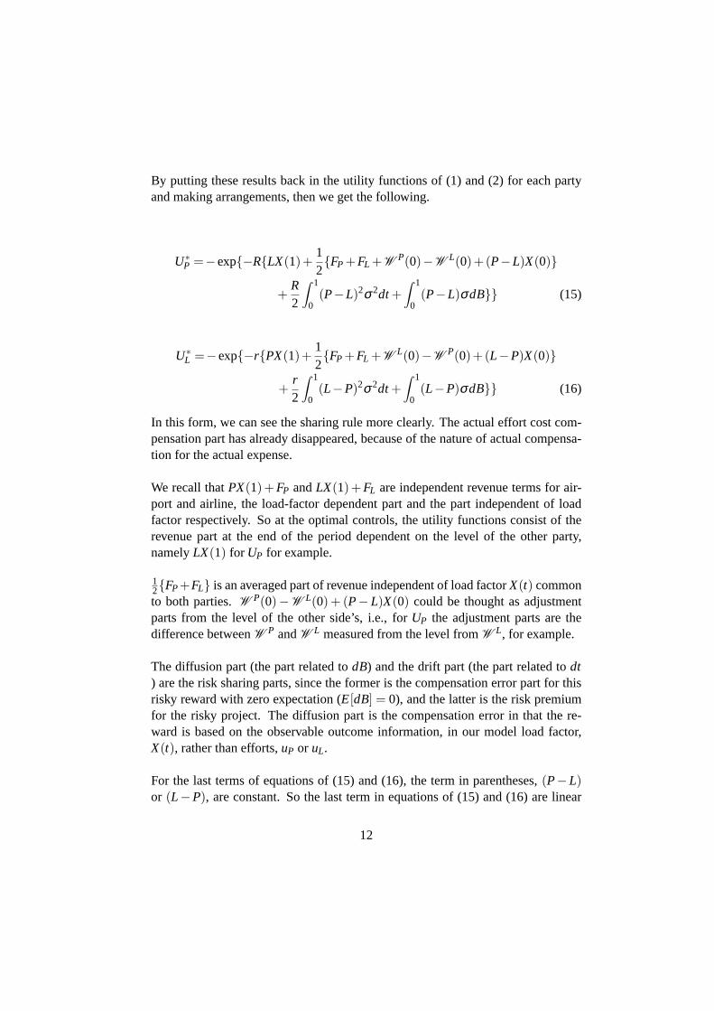
By putting these results back in the utility functions of (1) and (2) for each partyand making arrangements, then we get the following.

U∗P =−exp−RLX(1)+

12FP +FL +W P(0)−W L(0)+(P−L)X(0)

+R2

∫ 1

0(P−L)2σ2dt+

∫ 1

0(P−L)σdB (15)

U∗L =−exp−rPX(1)+

12FP +FL +W L(0)−W P(0)+(L−P)X(0)

+r2

∫ 1

0(L−P)2σ2dt+

∫ 1

0(L−P)σdB (16)

In this form, we can see the sharing rule more clearly. The actual effort cost com-pensation part has already disappeared, because of the nature of actual compensa-tion for the actual expense.

We recall thatPX(1)+FP andLX(1)+FL are independent revenue terms for air-port and airline, the load-factor dependent part and the part independent of loadfactor respectively. So at the optimal controls, the utility functions consist of therevenue part at the end of the period dependent on the level of the other party,namelyLX(1) for UP for example.

12FP+FL is an averaged part of revenue independent of load factorX(t) commonto both parties.W P(0)−W L(0) + (P− L)X(0) could be thought as adjustmentparts from the level of the other side’s, i.e., forUP the adjustment parts are thedifference betweenW P andW L measured from the level fromW L, for example.

The diffusion part (the part related todB) and the drift part (the part related todt) are the risk sharing parts, since the former is the compensation error part for thisrisky reward with zero expectation (E[dB] = 0), and the latter is the risk premiumfor the risky project. The diffusion part is the compensation error in that the re-ward is based on the observable outcome information, in our model load factor,X(t), rather than efforts,uP or uL.

For the last terms of equations of (15) and (16), the term in parentheses,(P−L)or (L−P), are constant. So the last term in equations of (15) and (16) are linear

12

equation of final results,X(1).

The drift term and diffusion term are both weighted by(P− L), which are pro-ductivity ratio between the two parties by equations (13) and (14) in addition tovolatility(σ ) or variance(σ2) of the uncertainty.

If we do the (stochastic) integrations in the equations (15) and (16), we get thefollowings.

U∗P = −exp−RL+(P−L)σX(1)

+12FP +FL +W P(0)−W L(0)+(P−L)(1−2σ)X(0)

+R2(P−L)2σ2 (17)

U∗L = −exp−rP+(L−P)σX(1)

+12FP +FL +W L(0)−W P(0)+(L−P)(1−2σ)X(0)

+r2(L−P)2σ2 (18)

In this form too, we can confirm that the optimal sharing rules under the decentral-ized maximizations stated in Problem A are linear function of the final outcome.Also from the equations (15) and (16) with equations (13) and (14), we can confirmthat the drift and diffusion terms are weighted by the difference of productivity ra-tios between the two parities.

4.3 The Agreeable Sharing Rule

The derivedSP∗ andSL∗ above are not identical. So it is not possible for airport andairline to actually agree on a sharing rule with this difference remained. We needsome kind of framework to structure the agreement of two parties. So we introducethe following Assumption 3.

Assumption 3

13

In so far as for every numberε ∈ R+, there exist numbers,δ1 ∈ R+, aP ∈ R,δ2 ∈ R+ andaL ∈ R such that

|SL∗(r)−SP∗(R)| < ε and 0< |R−aP| < δ1 and 0< |r −aL| < δ2,

(namely,|SL∗(r)−SP∗(R)| → 0 asR→ aP andr → aL),

airport and airline can agree on a single sharing ruleS∗, which is defined as fol-lows.

SP∗(R) → S∗ asR→ aP

SL∗(r) → S∗ asr → aL

We call thisS∗ as an agreeable sharing rule.

Under Assumption 3, we have the framework for airport and airline to reach a sin-gle agreement out of the de-centralized utility maximizations in Problem A above.That is, if their risk aversions approach to some fixed numbers asymptotically andthe difference of|SP∗(R)−SL∗(r)| approaches to zero with them, then the two par-ties can reach a risk sharing rule contract which is optimal to both parties under thede-centralized utility maximizations in Problem A.

Next is the assumption about the cost differences between airport and airline in theequations (11) and (12).

Assumption 4We further assume that the optimal efforts of both airport and airline are costlessor negligibly minuscule. This means as follows.

cP(u∗P) = cL(u∗L) = 0 (cP(u∗P) ≈ 0, cL(u∗L) ≈ 0) (19)

Assumption 4 is a stringent assumption. By Assumption 2 and assumptions oncP,cL and f (uP,uL), we have unique optimal effort levels,u∗P andu∗L. The costs ofboth parties’ optimal effort levels are negligible by Assumption 4. Here we are nottrying to state this assumption is plausible. But rather we try to clarify that in ourde-centralized maximization model, the cost terms are very important to satisfyAssumption 3. As can be easily checked from the equations (11) and (12), onlywith Assumption 4, we have a possibility for the agreeable sharing rule definedin Assumption 3. In other words, unless Assumption 4 is satisfied, there is nochance for the two parties to agree on a single contract in our model even with the

14

agreement framework of Assumption 3. In other words, unless Assumption 4 issatisfied, there is no chance for the two parties to agree on a single contract in ourmodel.

Proposition 2If both parties’ risk aversion parameters (R and r) approach asymptotically to zerounder Assumption 3 and Assumption 4, airport and airline can agree on a sharingrule, which is derived as optimal sharing rules out of the de-centralized utilitymaximizations in Problem A and is the linear function of the final state of loadfactor. In this case, the agreeable optimal risk sharing ruleS∗ is as follows.

S∗ = (P−L)(1−σ)X(1)

+12FP−FL − (W P(0)−W L(0))+(P−L)X(0) (20)

Proof of Proposition 2When both parties’ risk aversion parameters asymptotically approach to zero, thismeans thatR→ 0 andr → 0 (aP ≡ 0 andaL ≡ 0 in Assumption 3)4. With Assump-tion 4 and from equations (11) and (12), we can easily deriveS∗ as in the equation(20).

With the result,|SL∗(r)−SP∗(R)| → 0. Hence with Assumption 3, airport and air-line can agree onS∗ as an optimal risk sharing rule sinceSP∗ andSL∗ are optimalfor airport and airline respectively.

Q.E.D.

This result is consistent to a certain degree with Romano (1994) and Bhattacharyyaand Lafontaine (1995). Although in a different modeling framework for doublehidden action/moral hazard problem (i.e., non-dynamic setting), they all show thatthere always exists a linear contract, which implements the second best (i.e., underdouble moral hazard) effort levels when both principal and agent are risk neutral.

However, our result contrasts Kim and Wang (1998a). They show that in non-dynamic setting, the optimal non-linear unique sharing rule under double moral

4Notice that risk parameters (R and r) being approaching asymptotically zero is not necessarilyequivalent to AP and AL becoming risk neutral. Risk aversion parameters being zero (R= r = 0) inCARA utility functions (U = −exp(−iy), i = R, r) means utility functions are all constant (U =−1), which is a special, more strict case of risk neutrality in general.

15

hazard with risk neutral principal and risk averse agent does not approach to thelinear contract as the agent’s risk aversion approaches to zero.

In our case, Proposition 2 shows that in dynamic setting, two parties can agreeon an optimal linear contract under double moral hazard in our decentralized util-ity maximizations if both parties’ risk aversion parameters asymptotically becomezero and Assumption 4 is satisfied.5

The equation (20) shows that the slope of the linear contract is the product of thetwo parts. One is(P−L), which is the difference of productivity of both parties,which can be seen from the equations (13) and (14)6. The other is the uncertaintylevel measured as(1−σ). The slope is the procuct of the two parts.

This means that if both parties’productivities are equal,P−L = 0, or if the diffu-sion rate is unity, 1−σ = 0, then the slope is zero. So both parties are equal-footingin productivity, then the compensation part dependent on the realized final outcomeof the optimal sharing rule disappears.

Also if the uncertainty in the project indicated by the diffusion rate of the Weinerprocess in our model is unity, then the compensation error part related to the re-alized final outcome,−(P−L)σX(1), of the optimal sharing rule just cancel outthe productivity difference compensation part elated to the realized final outcome,(P−L)X(1), resulting in the zero slope of the linear function of realized final out-come.

In both cases, the remaining optimal sharing rule is just the utility level adjustmentsconsisting only of parts not related to the realized final outcomeX(1).

In other cases, the sign of the slope of the term related the realized final outcomedepends on the signs of the two pars, the productivity differences(P−L) and un-certainty level measured as(1−σ). If (P−L)> 0 and(1−σ) > 0, and,(P−L)< 0and(1−σ) < 0, the slope is plus. On the other hand, ff(P−L) > 0 and(1−σ) < 0,and,(P−L) < 0 and(1−σ) > 0, the slope is minus.

5On the other hand, Kim and Wang (1998a) showed that under double moral hazard situation, ontheir model, the optimal sharing rule between risk neutral principal and risk averse agent is not linearcontract and that linear contract is not a limiting contract as agent’s risk aversion approaches to zero.In our case, the optimal contracts are linear contract and as both parties’ risk aversions asymptoticallyapproach to zero, they can agree on a limiting optimal linear contract.

6In non-dynamic double moral hazard setting for risk neutral principal and agent case, the slopeof the linear optimal sharing rule is the agent’s productivity.

16

As can be seen from these explanations, the slope of the linear function of theagreeable optimal sharing rule is the product made by the productivity difference(P−L) and the uncertainty level index(1−σ).

Based on the contents of Proposition 1 and Proposition 2, we can construct Propo-sition 3.

Proposition 3If we assume perfect symmetry, i.e., everything being same between the two con-tracting parties, in addition to Assumption 1 through 4, the risk sharing rule disap-pears completely in the double moral hazard situation in this setting.

Proof of Proposition 3Under the perfect symmetry, everything between two parties is same. This meansthat among other things

P = L,R= r,FP = FL

W P(0) = W L(0).

With these put in the equation (20), we have the following results

S∗ ≡ 0

Hence the risk sharing rule disappears completely with the additional perfect sym-metry assumption.

Q.E.D.

5 Numerical Illustration

5.1 Concrete Settings

Here we illustrate some of the structures we used in the preceding chapters. Firstwe show the concrete results for modelingX(t) for load factor during the contractperiod.

17

We assume the following concrete structures of functions7;

f (uP,uL) = uP +uL

cP(uP) =kP

2uP

2− P2

2kP

cL(uL) =kL

2uL

2− L2

2kL

dX(t) = (uP +uL)dt+σdB

We further assume

X(0) = 0.6886,σ = 0.056,uP = uL = 0.005 or 0.025.

The 5 sample paths ofX(t) for bothuP = uL = 0.025 (left graph) and 0.005 (rightgraph) cases are shown in the Figure 1.

(Figure 1 is about here.)

Also we simulated the X(1) results with 10,000 iterations. The simulated resultsare the Figure 2.


The mean and the standard deviation of the simulatedX(1) for uP = uL = 0.005 is;meanµ = 0.6411standard deviationσ = 0.0266.

The mean and the standard deviation of the simulatedX(1) for uP = uL = 0.025 is;meanµ = 0.7013standard deviationσ = 0.0194.

7The cost function could be negative in our settings like Schaettler and Sung (1993) and Kimand Wang (1998a). This could be explained if both parties are receiving some financial aid fromnational government, for example. This aid could be lump sum or volume based for the purposeof cost alleviation. In our example, we assume lump some financial aid to reduce the two parties’costs. This could be the case, if local government, which owns and leases land for both airline (officepremises) and airport (parking space) surrounding area of the airport, decreases its lease premium byfixed amount, the costs of airline and airport decrease accordingly by the same lump sum amount.

18

We can see the improvement of final load factor at the end of the period with moreefforts of both parties even if the initial load factor is the same.

5.2 Optimal Levels

By the assumptions and these numbers with equations (13) and (14), we can derivethe optimal efforts levels and optimal sharing rules.

u∗P =PkP

(21)

u∗L =LkL

(22)

Notice that these solutions satisfy Assumption 4. Namely, we have

cP(u∗P) =kP

2

(PkP

)2

− P2

2kP= 0

cL(u∗L) =kL

2

(LkL

)2

− L2

2kL= 0.

With the result of the optimal effort levels, we have optimal sharing rules. Theseare the equations (11) and (12) with concrete parameter values.

SP∗(X) = (P−L)(1−σ)X(1)+12FP−FL − (W P(0)−W L(0))+(P−L)X(0)

− R2(P−L)2σ2 (23)

SL∗(X) = (P−L)(1−σ)X(1)+12FP−FL − (W P(0)−W L(0))+(P−L)X(0)

+r2(L−P)2σ2 (24)

If both parties’ risk aversionsR andr asymptotically approach to 0, both canagree, based on Assumption 3, on the optimal sharing rule of the equation (20)

19

with concrete parameter values as follows.

S∗ = (P−L)(1−σ)X(1)

+12FP−FL − (W P(0)−W L(0))+(P−L)X(0) (25)

In Figure 3, we show that|SL∗−SP∗| → 0 asR→ 0 andr → 0 under the followingnumerical settings.

P = 0.055; kP = 11u∗P = P

kP= 0.005

L = 0.011; kL = 2.2u∗L = L

kL= 0.005

X(1) ∼ N(0.6411,0.02662)W P(0) = 1.1;W L(0) = 1FP = 11;FL = 10X(0) = 0.668


This means airport and airline can agree on an optimal sharing contractS∗ withconcrete paremater values as their risk aversion parameters asymptotically becomezero.

5.3 Diffusion Rate Effects

As the equation (20) and (25) indicate, the optimal agreeable contract , which islinear function of the final state, has the slope of the product of both parties’pro-ductivity differenceP−L and uncertainty (diffusion rate) level index 1−σ .

The productivity difference part of the slope is the part to level the productivity dif-ference dependent on the final state through the sharing rule. By this, the optimalagreeable sharing rule adjusts the revenue differences between two parties gener-ated by the productivity differences even if they share the common final outcome.

The uncertainty (diffusion rate) level index part of the slope is the part to adjust

20

the compensation error after adjusting the productivity differences. Compensationerror adjustment is necessary, since the sharing is based on the uncertain outcomenot on the efforts actually performed. In our model, the productivity differenceadjustment part has the same termP−L in the opposite sign. So the compensationerror part in the slope is the form of1−σ , not justσ .

If the diffusion is zero, then no uncertainty entails. Only the productivity differ-ences matter. So the slope is just the productivity difference adjustment,P−L. Ifthe diffusion is unityσ = 1 in our model, then the compensation error adjustmentis just the same as the countering productivity difference. So the slope is zero. Inthis case, the optimal sharing rule has no part with the final outcomeX(1) . Onlythe fixed income partFP andFL, and the initial condition parts are involved in theoptimal sharing rule. Therefore the optimal agreeable sharing rule has only theattributes of the two parties that are not dependent on the final outcomeX(1).

In Figure 4, we illustrate the optimal sharing contractS∗ linear in X(1), the loadfactor at the end of the contract period with the impact of the diffusion rateσ .


As diffusion rateσ increases, the slope of optimal contractS∗ decreases. Thismean that as the volatility of Brownian motion increases, the compensation errornecessary part in the optimal sharing rule becomes large. If the compensation erroroverwhelms the positive impact of load factorX(1) impact, then the slope of thelinear sharing rule becomes negative.

More specifically, if diffusion rateσ is unity, then the slope is zero. This meansthat the compensation error part just negate the productivity difference adjustmentin the slope, ifσ = 1. In this case, the optimal sharing rule has only the parts thatdo not depend on the load factor at the endX(1), as we explained above.

If diffusion rateσ is less than 1, the effect of load factorX(1) on the sharing ruleis greater than the effect of compensation error, which is the opposite sign of theeffect of load factor, resulting from the diffusion rateσ . So the slope ofS∗(X(1))is positive. The contradicting effect between that withX(1) and that withσ can beseen from the equation (9) and (10). But on the other hand, if the diffusion rateσis greater than 1, the negative compensation error effect overwhelms the positiveeffect of load factor improvement, hence the negative slope of the optimal sharingcontract.

21

Under the agreeable sharing rule, we have the optimal utility functions.

U∗P(X(1),σ) = −exp−RL+(P−L)σX(1)

+12FP +FL +W P(0)−W L(0)+(P−L)(1−2σ)X(0)

(26)

U∗L (X(1),σ) = −exp−rP+(L−P)σX(1)

+12FP +FL +W L(0)−W P(0)+(L−P)(1−2σ)X(0)

(27)

In Figure 5, we show the visualized utility level with the final outcome of loadfactorX(1) and the diffusion rateσ , settingR= r = 10−4.


As we can see from the left graph of Figure 5, the impact of increased diffusionrate onUP∗ is relatively simple. As diffusion rate increases, so does the impact

of X(1), i.e., the slope∂UP∗(X(1),σ)∂X(1) . The slope is always positive. The intercept

UP∗(0,σ), on the other hand, decreases asσ increases.

In the right graph of Figure 5, the impact onUL∗ is relatively complex in our

numerical example. Asσ increases, the impact ofX(1), i.e., the slope∂UL∗(X(1),σ)∂X(1) ,

is decreasing. Ifσ ≥ 1.25, the slope becomes negative and continue to decrease.The interceptUL∗(0,σ), on the other hand, increases asσ increases.

Now we turn to the total utilities level for both AP and AL. With the above results,we can gauge the impact of increased uncertainty and the end-of-period load factorimprovement on the total utilities level. To specify these impacts, we can calculatethe derivatives of the total utilities with respect toσ andX(1).

22

U∗A = U∗

P +U∗L

∂U∗A

∂X(1)= U∗

P[−RL+(P−L)σ]+U∗L [−rL+(P−L)σ] > 0

∂U∗A

∂σ= U∗

P(−R)(P−L)(X(1)−X(0))+U∗L (−r)(L−P)(X(1)−X(0)) ≈ 0

Notice that sinceR≈ 0 andr ≈ 0, we have the last results.

Figure 6 is the graph forU∗A = U∗

P +U∗L with X(1) andσ . The slope ofU∗

A withrespect toX(1) is positive and the slope with respect toσ is almost zero.


The impact of uncertainty increase is almost zero with some perturbations, sincewe already assuming that the risk averse parameters approach asymptotically tozero. The impact of the final outcome improvement, on the other hand, has a posi-tive effedct on the total utilities level with some perturbations.

Because of risk averse parameters approaching to zero, the conflicting effects causedby diffusion rate changes on each party’s utility through the optimal agreeable shar-ing rule as depicted in Figure 5 are almost smoothed out in the total utilities levelas depicted in Figure 6. With some perturbations,σ changes have almost no effecton the total utilities level in Figure 6.

6 Concluding Remarks

We show that, under the double hidden action/moral hazard situation of de-centralizedutility maximizations based on the stochastic load factor process under additivelyseparable efforts assumption and convexity assumption about the relationship be-tween production and cost function, the optimal sharing structures are the linearfunction of the final state for both parties. In this case, the drift and diffusion termsare weighted by the difference of productivity between the two parities.

If we further assume that the costs of optimal effort are negligible and also assumeboth parties’ risk aversion parameters approach asymptotically to zero, then we

23

show that both parties can agree on a single optimal contract, which is also a linearfunction of final load factor.

Our finding is to some degree consistent with some of double hidden action/ moralhazard situation analysis of preceding literatures. Namely, if both parties are riskneutral, the linear function of the end-state is among the optimal sharing rules.

However, our result contrasts with Kim and Wang (1998a). They show, in non-dynamic setting, the optimal non-linear unique sharing rule under double moralhazard with risk neutral principal and risk averse agent does not approach to thelinear contract as the agent’s risk aversion approaches to zero.

We find that in dynamic setting, two parties can agree on an optimal linear contractunder double moral hazard in our decentralized utility maximizations if both par-ties’risk aversion parameters asymptotically become zero and optimal effort arenegligible, as we alread stated.

The optimal agreeable contract, which is linear function of the final state, has theslope of the product of both parties’productivity difference and uncertainty (dif-fusion rate) level index.

If the productivities are same between the two parties in our setting, there is no needto adjust their productivity difference by the optimal sharing rule. So the slope iszero. In this case, the optimal sharing rule has no part with the final outcome.

If the diffusion rate is unity in our model, then the compensation error adjustmentis just the same as the countering productivity difference adjustment. So the slopeis zero. In this case, the optimal sharing rule has no part with the final outcome.

In addition, if everything is symmetric, then the risk sharing rule disappears com-pletely.

With numerical examples, we show the sample paths for load factor processes gen-erated according to underlying Weiner process. The improving effects of effortincreases of both parties on the end-of-period load factors are provided. Also weshow the convergence to the agreeable sharing rule as both parties’ risk averse pa-rameters get asymptotically to zero.

We show that the complex effect of increased diffusion rate on the linear functionof the agreeable optimal sharing rule. The impacts on total utilities level are rel-

24

atively simple. The impacts of diffusion rate increase on total utilities are almostzero. The increase of final outcome has a positive effect on the total utilities level.

As one example of the next steps, we can look into the other double hidden action /moral hazard model of utility maximizations, which is other than our de-centralizedmodel. This direction is in line with the past literature. However, in the stochasticprocess model, this would require much more mathematical sophistication.

Also we can try to relax the restrictive assumptions on the functions, includingfandcP andcL. For example, we assume they are not function of timet. This wouldalso require much more rigorous theoretical treatments. Since even in our simplemodel with restrictive functions, we can show some results, we should try to bal-ance clarity and reality when pursuing in this direction.

In the context of network industries of routes and airports, another important nextstep could be to try to link the abstract efforts in our model to concrete tools of theaviation and airport industries, such as pricing, routing and frequencies, so that wecan more directly see the interaction within the airport and airline vertical relation-ship in more realistic settings.

7 Acknowledgement

The author expresses gratitude to Professor Naoki Makimoto (University of Tsukuba)for valuable comments. Any remaining errors are entirely the author’s responsi-bility.

Financial supports from the Airport Environment Improvement Foundations, Kan-sai International Airport Co., Ltd., Narita International Airport Co., Ltd. and JapanAirport Terminal Co., Ltd. are gracefully acknowledged.

A Appendix A Proof of Proposition 1

As already stated, under Assumption 1, functionf (uP,uL) can be treated com-pletely separately forup anduL in applying Theorem 3.1 and 4.1 for necessarycondition and Theorem 5.1 for sufficient conditions in Schaettler and Sung (1993),since there is no interacting relationship betweenuP anduL, i.e., equation (8). So

25

for example, in solving equation(5) we can apply these theorems only touL, whilein solving equation (4) we can apply these theorems only touP.

We show the proof of the derivation ofSP(X) only, since that ofSL(X) is basicallysame. Also to avoid the just duplication, we only describe the main part of thederivation in the following equations.

maxSP(X),uP,uL

E[−exp−RPX(1)+FP−SP(X)−∫ 1

0cP(uP)dt] (4)

s.t.


uL ∈ argmaxuL

E[−exp−rLX(1)+FL +SP(X)−∫ 1

0cL(uL)dt] (5)

First, we apply Theorem 3.1 and 4.1 in Schaettler and Sung (1993) to the maxi-mization problem of equation (5) under equation (3) holdinguP constant. Noticethat indX(t) we have alsouL.

As usual, we assume theSP(X) has the following structure.

SP(X) = SP1(X)+

∫ 1

0α(s,X)ds+

∫ 1

0β (s,X)dXs

From equation (5), structure ofSP(X) andX(1) = X(0)+∫ 1

0 f (uP,uL)dt+∫ 1

0 σdBwith some arguments suppressed, the utilityUL becomes as follows;

UL =−exp−r(LX(0)+FL +SP1(X)

−∫ 1

0r(L f (uP,uL)+α +β f (uP,uL)−cL(uL))dt

−∫ 1

0r(L+β )σdB

By applying Theorem 3.1 in Schaettler and Sung (1993), there existFt -adaptedprocessVt and∇Vt ,

∫ 10 | ∇Vtσ |2 dt < ∞ a.e., such thatu∗L ∈ U is optimal control

if and only if

26

∇Vt f (uP,u∗L)− rσ2(L+β )

+Vt−r(L+β ) f (uP,u∗L)− rα + rcL(u∗L)+12

r2σ2(L+β )2

≡ maxuLinU

∇Vt f (uP,uL)− rσ2(L+β )

+Vt−r(L+β ) f (uP,uL)− rα + rcL(uL)+12

r2σ2(L+β )2

for almost all(t,ω) ∈ [01]×Ω. Furthermore, the value processVt has an Ito dif-ferential of the form

Vt = V0−∫ t

0[∇Vs f (uP,u∗L)− rσ2(L+β )

+Vt−r(L+β ) f (uP,u∗L)− rα + rcL(u∗L)

+12

r2σ2(L+β )2]ds+∫ t

0∇VsdXs.

Vt , ∇Vt and∇Vt are value functions of stochastic process as defined in AppendixA in Schaettler and Sung (1993).

Using∇Vt ≡ ∇Vt −Vtr(L+β ), we can get thecL related part as follows;

∇Vt f (uP,uL)+VtrcL(uL)

FOC for maximization for this, we have the following;

∇Vt

rVt= − c′L(u

∗L)

∂ f (uP,u∗L)∂uL

As usual, we define the following certainty equivalent value processWt as follows;

Wt = −1r

ln(−Vt)

With some arrangements, we get the following equation.

dWt = cL(u∗L)dt+r2

( ∇Vt

rVt

)2σ2dt+∇Vt

rVtσdB

− (αdt+βdX)−LdX

27

So we getSP(X) as follows.

SP(X) = −(W L1 −W L

0 )+SP1(X)−L(X(1)−X(0))

+∫ 1

0cL(u∗L)dt+

r2

∫ 1

0

(c′L(u

∗L)


)2

σ2dt

+∫ 1

0

c′L(u∗L)


σdB

Here we useW Lt instead ofWt for notational clarity in the following further deriva-

tion of SP(X).

By the Theorem 5.1 in Schaettler and Sung (1993), thisSP(X) satisfies the suffi-cient condition of maximizing the equation (4) with holdinguP as a constant.

Rearranging the terms and defining newlyFP(X), α ′ andβ ′, we get the following.

SP(X) =− (W L1 −W L

0 )+SP1(X)−L(X(1)−X(0))

+∫ 1

0[cL(u∗L)+

r2

∫ 1

0

(c′L(u

∗L)


)2

σ2−

(c′L(u

∗L)


)f (uP,u∗L)]dt

+∫ 1

0

c′L(u∗L)


dX (A.1)

≡ FP(X)+∫ 1

0α ′dt+

∫ 1

0β ′dX (A.2)

FP(X) ≡−(W L1 −W L

0 )+SP1(X)−L(X(1)−X(0))

Now we turn to the maximization of the equation (4) by choosinguP, which is nowa controlling variable rather than a constant. We putSP(X) in the equation (4),rearrange terms and have the following equation.

28

UP =−exp−R(PX(0)+FP−FP(X))

+∫ 1

0R(β ′−P) f (uP,u∗L)+cP(uP)+α ′dt

+∫ 1

0R(β ′−P)σdB

We apply Theorem 3.1 again here. Then there existV Pt and∇V P

t ,∫ 1

0 | ∇V Pt σ |2

dt < ∞ a.e., such thatu∗P ∈ U is optimal control if and only if

∇V Pt f (u∗P,u∗L)+Rσ2(β ′−P)

+V Pt R(β ′−P) f (u∗P,u∗L)+α ′ +cP(u∗P)+

12

R2σ2(β ′−P)2

≡ maxuPinU

∇V Pt f (uP,u∗L)−Rσ2(β ′−P)

+V Pt R(β ′−P) f (uP,u∗L)+α ′ +cP(uP)+

12

R2σ2(β ′−P)2

for almost all(t,ω) ∈ [0,1]×Ω. Furthermore, the value processV Pt has an Ito

differential of the form

V Pt = V P

0 −∫ t

0[∇V P

s f (u∗P,u∗L)+Rσ2(β ′−P)

+V Pt R(β ′−P) f (u∗P,u∗L)+α ′ +cP(u∗P)

+12

R2σ2(β ′−P)2]ds+∫ t

0∇V P

s dXs].

We can construct the following.

∇V Pt ≡ ∇V P

t +RV Pt (β ′−P)−RV P

tc′L(u∗L)∂ f (uP,u∗L)

∂uL

With this, we get theuP related part as follows;

∇V Pt f (uP,u∗L)+V P

t RcP(uP)

FOC for maximization for this, we have the following;

∇V Pt

RVt= − c′P(u∗P)

∂ f (u∗P,u∗L)∂uP

29

Here, we define the following certainty equivalent value processW Pt as follows;

W Pt = −1

Rln(−V P

t )

With some arrangements, we get the following equation.

dW Pt = cP(u∗P)dt+

R2 ∇V P

t

RVt+(β ′−P)2σ2dt− ∇V P

t

RV Pt

+(β ′−P)σdB

− (α ′dt+β ′dX)−PdX

By integrating and usingSP(X) = FP(X)+∫ 1

0 α ′dt+∫ 1

0 β ′dX, we have as follows.

SP(X) =W P1 −W P

0 +FP(X)+P(X(1)−X(0))

−∫ 1

0cP(u∗P)dt− R

2

∫ 1

0

(c′L(u

∗L)

∂ f (u∗P,u∗L)∂uL

− c′P(u∗P)∂ f (u∗P,u∗L)

∂uP

)2

σ2dt

+∫ 1

0

(c′L(u

∗L)

∂ f (u∗P,u∗L)∂uL

− c′P(u∗P)∂ f (u∗P,u∗L)

∂uP

)σdB

Notice that the terminal conditions are thatLX(1) + FL + SP1(X) = W L(1) and

PX(1)+FP−W P(1)−W P(0)+FP(X)+P(X(1)−X(0))= W P(1). With theseconditions and by expandingFP(X), we get the following.

SP(X) =PX(1)−LX(1)+12FP−FL − (W P(0)−W L(0))− (P−L)X(0)

−∫ 1

0cP(u∗P)dt− R

2

∫ 1

0

(c′P(u∗P)∂ f (u∗P,u∗L)

∂uP

− c′L(u∗L)∂ f (u∗P,u∗L)

∂uL

)2

σ2dt

−∫ 1

0


∂uP

− c′L(u∗L)∂ f (u∗P,u∗L)

∂uL

)σdB (A.3)

By the same process, we get the following.

30

SL(X) =PX(1)−LX(1)+12FP−FL − (W P(0)−W L(0))− (P−L)X(0)

+∫ 1

0cL(u∗L)dt+

r2

∫ 1

0

(c′L(u∗L)∂ f (u∗P,u∗L)

∂uL

− c′P(u∗P)∂ f (u∗P,u∗L)

∂uP

)2

σ2dt

+∫ 1

0


∂uL

− c′P(u∗P)∂ f (u∗P,u∗L)

∂uP

)σdB (A.4)

Putting these back in the utility functions ofUP andUL, the resulting utility func-tions at the optima are the followings.


12FP +FL +W P(0)−W L(0)+(P−L)X(0)

+R2

∫ 1

0


∂uP

− c′L(u∗L)∂ f (u∗P,u∗L)

∂uL

)2

σ2dt

+∫ 1

0


∂uP

− c′L(u∗L)∂ f (u∗P,u∗L)

∂uL

)σdB (A.5)


12FP +FL − (W P(0)−W L(0))− (P−L)X(0)

+r2

∫ 1

0


∂uL

− c′P(u∗P)∂ f (u∗P,u∗L)

∂uL

)2

σ2dt

+∫ 1

0


∂uL

− c′P(u∗P)∂ f (u∗P,u∗L)

∂uP

)σdB (A.6)

Notice that, as we already mentioned, by Theorem 5.1 in Schaettler and Sung(1993), theSP(X) andSL(X) above satisfy the sufficient condition of the (relaxed)maximization problems ofUP in the equation (4) andUL in the equation (6).

During the deriving process ofu∗L, for example, the airport’s relaxed problem re-quiresuL to satisfy the following equation of dynamic programming according to

31

Theorem 5.1 in Schaettler and Sung (1993).

0≡∂W P(t,X)∂ t

+12

∂ 2W P(t,X)∂X2 − R

2

(∂W P(t,X)∂X

)2σ2

+maxuL

[∂W P(t,X)

∂X f (uP,uL)+Rβ ′σ2dt

−(cp(uP)+cL(uL)+

R+ r2

β ′2σ2)dt] (A.7)

From the maximization foru∗L and noticingβ ′ = β ′(t,X), we get the following.

∂W P(t,X)∂X

=c′L(u∗L)∂ f (uP,u∗L)

∂uP

(A.8)

The dynamic programming equation above is separable and it is well known howto solve it. Noticing the terminal condition ofW P(1) = LX(1) + 1

2FP + FL +W P(0)−W L(0)+(P−L)X(0), we get the following.

W P(t,X) =LX

+R2

L2σ2−β ′ f (uP,u∗L)

− R− r2

β ′2σ2 +cL(u∗L)+cP(uP))(t −1)

+12FP +FL +W P(0)−W L(0)+(P−L)X(0) (A.9)

From this, we can derive the following.

∂W P(t,X)∂X

=c′L(u∗L)∂ f (uP,u∗L)

∂uL

= L (A.10)

From this result along with the assumptions of convexity ofcL and concavity offand Assumption 2, the optimal controlu∗L is unique.

Also u∗L is constant across the period, namelyu∗L(t) ≡ u∗L, since neithercL nor fdepends on timet by assumptions.

32

The same process can be performed foru∗P. Then we get the following.

∂W L(t,X)∂X

=c′P(u∗P)∂ f (u∗P,uL)

∂uP

= P (A.11)

Therefore the optimal controls,u∗P andu∗L, are unique and constant during the pe-riod.

Putting these results back in (A.3) and (A.4), we have the following.

SP(X) =PX(1)−LX(1)+12FP−FL − (W P(0)−W L(0))− (P−L)X(0)

−∫ 1

0cP(u∗P)dt− R

2

∫ 1

0(P−L)2σ2dt

−∫ 1

0(P−L)σdB (A.12)

SL(X) =PX(1)−LX(1)+12FP−FL − (W P(0)−W L(0))− (P−L)X(0)

+∫ 1

0cL(u∗L)dt+

r2

∫ 1

0(L−P)2σ2dt

+∫ 1

0(L−P)σdB (A.13)

If the integrations in these equations are executed, we have the followings.

SP∗(X) =(P−L)(1−σ)X(1)+12FP−FL − (W P(0)−W L(0))+(P−L)X(0)

−cP(u∗P)− R2(P−L)2σ2 (A.14)

SL∗(X) =(P−L)(1−σ)X(1)+12FP−FL − (W P(0)−W L(0))+(P−L)X(0)

+cL(u∗L)+r2(L−P)2σ2 (A.15)

33

These are exactly the equations (11) and (12) as indicated.With these results, we have theU∗

P andU∗L as follows.


12FP +FL +W P(0)−W L(0)+(P−L)X(0)

+R2

∫ 1

0(P−L)2σ2dt+

∫ 1

0(P−L)σdB (15)


12FP +FL +W L(0)−W P(0)+(L−P)X(0)

+r2

∫ 1

0(L−P)2σ2dt+

∫ 1

0(L−P)σdB (16)

By doing the integrations of these equations, we have the followings.

U∗P = −exp−RL+(P−L)σX(1)

+12FP +FL +W P(0)−W L(0)+(P−L)(1−2σ)X(0)

+R2(P−L)2σ2 (17)

U∗L = −exp−rP+(L−P)σX(1)

+12FP +FL +W L(0)−W P(0)+(L−P)(1−2σ)X(0)

+r2(L−P)2σ2 (18)

These are exactly the equations (17) and (18) as indicated.

Q.E.D.

34

References

Barbot, C., June 2009. Vertical relationship between airports and airlines: Is there atrade-off between welfare and competitiveness? ATRS 2009 Abu Dhabi workingpaper.

Bhattacharyya, S., Lafontaine, F., 1995. Double-sided moral hazard and the natureof share contract. RAND Journal of Economics 26, 761–781.

Borch, K., 1962. Equilibrium in a reinsurance market. Econometrica 30, 424–444.

Feng, J., Fu, X., Summalee, A., 2010. Airport-airline cooperation under demanduncertainty. ATRS 2010 paper 150 presentation only.

Hihara, K., March 2008. Numerical analysis on payoff of load factor guaranteemechanism for noto airport. Transportation Research, 2007 FY Annual of JapanSociety of Transportation Studies (in Japanese), pp.169–178.

Hihara, K., November 2010. Analysis on airport-airline relationship with risksharing contract. University of Tokyo working paper GraSPP-DP-E-10-001 andITPU-DP-E-10-001.

Holmstrom, B., Milgrom, P., 1987. Aggregation and linearity in the provision ofintertemporal incentives. Econometrica 55, pp.303–328.

Kim, S. K., Wang, S., 1998a. Linear contracts and the double moral hazard. Journalof Economic Theory 82, 342–378.

Kim, S. K., Wang, S., 1998b. Linear contracts and the double moral hazard. HongKong University of Science and Technology working paper.

Mirrlees, J., 1979. Moral hazard and unobservable behavior. Bell Journal of Eco-nomics 10, 74–91.

Mueller, H. M., 1996. The first best sharing rule in the continuous time principalagent model with exponential utility. Stockholm School of Economics workingpaper series No 145.

Mueller, H. M., 1998. The first best sharing rule in the continuous-time principal-agent problem with exponential utility. Journal of Economic Theory 79, 276–280.

Oum, T. H., Fu, X., June 2009. Effects of airport-airline vertical relationship. ATRS2009 Abu Dhabi working paper.

35

Rogerson, W. P., 1985. The first-order approach to principal-agent problems.Econometrica 53, 1357–1367.

Romano, R. E., 1994. Double moral hazard and resale price maintenance. RandJournal of Economics 25, 455–466.

Schaettler, H., Sung, J., 1993. The first-order approach to the continuous-timeprincipal-agent problems with exponential utility. Journal of Economic Theory61, 331–371.

Schaettler, H., Sung, J., 1997. On optimal sharing rules in discrete- and continuous-time principal-agent problems with exponential utility. Journal of Economic Dy-namics and Control 21, 551–574.

Zhang, A., Fu, X., Yang, H., 2010. Revenue sharing with multiple airlines andairports. Transportation Research Part B forthcoming.

36

Figure 1 5 Sample Paths for Load Factor State Variable, X(t)

Left graph for u_P=u_L=0.005, Right graph for u_P=u_L=0.025

Figure 2 Simulated Paths for Load Factor State Variable, X(t)

Left graph for u_P=u_L=0.005, Right graph for u_P=u_L=0.025; each 10 000 iterationseach 10,000 iterations

Convergence into a Risk Sharing Contract

0

0.5

1

1.5

0

0.5

1

1.50

0.2

0.4

0.6

0.8

1

1.2

1.4

1.6

1.8

x 10-6

R

SP, S

L → S

* [|S

L - S

P| → 0, as R, r → 0]

r

|SL -S

P|

Figure 3

Figure 4 Optimal Contract S* Linear in X(1) ith Diff i R t ( )

0.52

Optimal Linear Contract S*(X(1), )

with Diffusion Rate (σ)

0.5

0.51

0.48

0.49

0 45

0.46

0.47

S*

0.43

0.44

0.45

1

1.5

2

0.42

0 0.1 0.2 0.3 0.4 0.5 0.6 0.7 0.8 0.9 1

0

0.5

1

X(1)

Figure 5 U_P* and U_L* with X(1) and σ

Figure 6 Total Utilities with X(1) & σFigure 6. Total Utilities with X(1) & σ

An Analysis on Airport-Airline Vertical Relationships with ...

Documents

Transcript of An Analysis on Airport-Airline Vertical Relationships with ...