Adaptive Dynamic Nelson-Siegel Term Structure Model with

Applications

Ying Chena Linlin Niub,c∗

aDepartment of Statistics & Applied Probability, National University of SingaporebWang Yanan Institute for Studies in Economics (WISE), Xiamen University

cMOE Key Laboratory of Econometrics, Xiamen University

Abstract

We propose an Adaptive Dynamic Nelson-Siegel (ADNS) model to adaptively fore-

cast the yield curve. The model has a simple yet flexible structure and can be safely

applied to both stationary and nonstationary situations with different sources of change.

For the 3- to 12-months ahead out-of-sample forecasts of the US yield curve from 1998:1

to 2010:9, the ADNS model dominates both the dynamic Nelson-Siegel (DNS) and ran-

dom walk models, reducing the forecast error measurements by between 30 and 60

percent. The locally estimated coefficients and the identified stable subsamples over

time align with policy changes and the timing of the recent financial crisis.

Keywords: Yield curve, term structure of interest rates, local parametric models, fore-

casting

JEL Classification: C32, C53, E43, E47

∗Corresponding author. Linlin Niu, Rm A301, Economics Building, Xiamen University, 361005, Xiamen,

China. E-mail: llniu@xmu.edu.cn.

1 Introduction

Interest rates are important in economies. They are not only used by households, firms

and financial institutions as primary input factors in making many economic and financial

decisions, but they are also used by central banks in their conduct of monetary policy in

order to fulfill policy goals for social investment, inflation and unemployment. The yield

curve, which is also called the term structure of interest rates, illustrates the relationship

between interest rates and time to maturities, i.e., the remaining time until a bond expires,

which can vary from a few days to many years. Compared with individual interest rates,

the yield curve is more important as it provides rich information about interest rates for

different maturities. The long-term interest rate is the weighted expectation of future

short-term interest rates adjusted for risks and risk compensation. The shape of the yield

curve reflects the market’s expectation on monetary policy and economic conditions. The

average yield curve is upward sloping, i.e., the longer the time to maturity, the higher the

interest rate. An inverted slope of the yield curve often anticipates economic recession, as

happened in each occasion in the US economy during the last four decades. Moreover, the

constantly growing derivatives market also make it necessary to understand the dynamics

of the yield curve over time in order to price the interest rate derivatives. Hence yield curve

forecasting has gained the attention of scholars and practitioners alike. Nevertheless, it

is not an easy task, and it is often found that the theoretically sophisticated models such

as the no-arbitrage or equilibrium term structure models forecast poorly, compared with a

simple random walk model (see Duffee, 2002; Duffee, 2011).

As opposed to the class of no-arbitrage and equilibrium models with theoretical under-

pinnings, there are reduced-form models based on a statistical approach, where interest

rates are often modeled with a univariate time series or a multivariate time series. The uni-

variate class includes the random walk model, slope regression model, and the Fama-Bliss

forward rate regression model (Fama and Bliss, 1987), where interest rates are modeled

for each term of maturity individually. One cannot, however, efficiently explore the cross-

sectional dependence of interest rates of different maturities for estimation and forecasting

purposes. The multivariate class includes the vector autoregressive (VAR) models and the

error correction models (ECMs), where interest rates of several maturities are considered

simultaneously to utilize the dependence structure and cointegration. However, this class

is subject to the curse of dimensionality, requiring the inclusion of more maturities and,

hence, cannot provide a complete view of the whole curve.

Alternatively, the recent advancement of factor models enables the modeling and forecast-

ing of the yield curve as a whole, where essential factors are extracted from the available

yield curves, and the forecast is based on these resultant low dimensional factors. The

factor approach retains the dependence information and is relatively easy to implement.

2

Among others, Diebold and Li (2006) propose a dynamic model based on the Nelson-Siegel

factor interpolation (Nelson and Siegel, 1987), and show that the model not only keeps

the parsimony and goodness-of-fit of the Nelson-Siegel interpolation, but also forecasts well

compared with the traditional statistical models. This dynamic Nelson-Siegel (DNS) model

has since become a popular forecasting tool of the yield curve. Instead of directly forecast-

ing the yield curve, the DNS model extracts three factors via Nelson-Siegel factor loadings.

The factors represent the level, slope and curvature of the yield curve. The evolutions of the

factors are represented with either an autoregressive (AR) model for each individual factor

or with a vector autoregressive (VAR) model for the three factors simultaneously. Given

the forecasts of the factors and the fixed loadings, one can obtain the yield curve forecasts.

Diebold and Li (2006) show that the AR(1) model specification performs better than many

alternatives, including the VAR specification, as well as the univariate and multivariate

time series models mentioned above.

However, we find that the recommended AR (1) model is deficient once the empirical

features of the factors are considered. The factors, like many other financial variables, are

very persistent. As an illustration, Figure 1 displays the time evolution of the Nelson-Siegel

factor of level and its sample autocorrelations. The factor is extracted from the US yield

curve data between 1983:1 to 2010:9, which we will describe in the next section. It shows

that the level factor has a long memory, with the sample autocorrelations hyperbolically

decaying up to lag 100. The AR(1) model, albeit a good forecast performance compared

with the alternative models, is unable to capture the persistence characteristics of the time

series.

[Figure 1. Time Plot of the Nelson-Siegel Level Factor and its Sample Autocorrelation

Function]

Naturally, persistence may be modeled with a long memory view using, for example, frac-

tionally integrated processes, see Granger (1980), Granger and Joyeux (1980) and Hosking

(1981). Note that these models rely on a stationary assumption in that the model pa-

rameters are assumed to be constant over time. Alternatively, a short memory view can

be employed, which says persistence can also be spuriously generated by a short memory

model with heteroscedasticity, structural breaks or regime switching, see Diebold and Inoue

(2001) and Granger and Hyung (2004). In other words, the fitted model is assumed to

hold only for a possibly short time period and the evolution of the local subsample can be

represented by a simple structural model, though the dynamics are changing from one time

period to another. In the literature about interest rates, several nonstationary models have

been proposed for yield curve modeling, see Ang and Bekaert (2002) and Bansal and Zhou

3

(2002) for regime shifts, Guidolin and Timmermann (2009) for the regime switching VAR

model, and Ang, Boivin, Dong and Loo-Kung (2011) for a monetary policy shift in a no-

arbitrage quadratic term structure model. The question is, which view is more appropriate:

a stationary model with long memory or a nonstationary model with a simple structure but

time-varying parameters?

It appears that the short memory view is quite realistic and easily understood in the

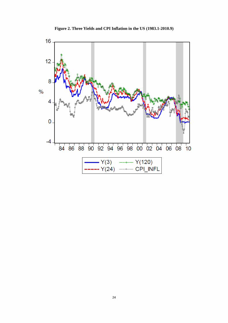
context of business cyclical dynamics, policy changes and structural breaks. Figure 2 plots

the monthly data, from 1983:1 to 2010:9, of three interest rates, with maturities of 3 months,

24 months and 10 years. The gray dashed line with circles shows the CPI inflation, which is

an important macroeconomic factor affecting nominal interest rates. The shaded bars mark

the three NBER recessions during the sample period: namely 1990:7-1991:3, 2001:3-2001:11

and 2007:12-2009:6. Over the whole sample period, interest rates show an obvious downward

trend. However, once we look at each subsample, separated by the three recessions, they

appear more stationary. Although the recession periods may not be the best divisions to

isolate stationary periods, statistically or economically, the point here is to show that there

may exist subsamples where the interest rates are approximately stationary and that can

be modeled sufficiently well with simple autoregressive processes. Our study employs the

methodology in Chen, Hardle and Pigorsch (2010) to detect divisions in real time.

[Figure 2. Three Yields and the CPI Inflation in the US (1983.1-2010.9)]

In the volatility forecasting literature, Chen et al. (2010) propose a local AR (LAR) model,

that allows for time-varying parameters, to model the seemingly persistence of volatility with

a short memory view. With time-varying parameters, the LAR model is flexible and able

to account for various changes of different magnitudes and types including both sudden

jumps or smoothed changes. Moreover, in terms of out-of-sample prediction, it performs

better than several alternative models including long memory models and some regime

switching models. A direct application of the LAR(1) model for yield curve forecast is apt.

However, as interest rate movements are closely related to macroeconomic conditions (see

Taylor, 1993; Mishkin, 1990; Ang and Piazzesi, 2003), it is more appropriate to widen the

scope of the LAR model by introducing macroeconomic variables such as inflation, growth

rate, etc.

In our study, we develop a new model to adaptively forecast the yield curve. It extracts

Nelson-Siegel factors cross-sectionally as in the DNS model. Then a local autoregressive

model with exogenous variables (LARX) is adopted to fit each factor dynamically. The

rationale is that, to conduct an estimation at any point of time, we take all available past

4

information and find a subsample where the observations included can be well represented by

a local stationary model with approximately constant parameters. In other words, there are

not any kind of significant changes in the estimation window. We then forecast the factors

as well as the yield curve based on the fitted model. We name it the adaptive dynamic

Nelson-Siegel (ADNS) model. At each point of time, this resulting model is a DNS model

over the detected stable subsample, where the dynamics of each factor are described by

an AR(1) process with exogenous variables. The adaptive procedure of stable subsample

detection is crucial for this model to distinguish it from the DNS model with predetermined

sample length. We investigate the performance of this proposed model in real data analysis,

and compare it with popular alternative models including the DNS and the random walk

models. We show the substantial advantage gained from using the adaptive approach in

forecasting, and bring useful insights in diagnosing yield dynamics with the produced stable

intervals and parameter evolvements.

The rest of the paper is organized as follows. Section 2 describes the data used. Section

3 presents the ADNS forecast model with a detailed discussion on the local model for each

factor. Section 4 reports the real data analysis and forecast comparison with alternative

models. Section 5 concludes.

2 Data

We use US Treasury zero-coupon-equivalent yield data with 15 maturities: 3, 6, 9, 12, 18,

24, 30, 36, 48, 60, 72, 84, 96, 108 and 120 months, from 1983:1 to 2010:9. The short-term

yields of 3 and 6 months are converted from the 3- and 6-month Treasury Bill rates on a

discount basis, available from the Federal Reserve’s H.15 release of selected interest rates.

The remaining yields with maturities of integer years are taken from research data of the

Federal Reserve Board, as released by Gurkaynak, Sack and Wright (2007). We add the 9-,

18-, and 30-month yields interpolated according to the parameters provided in their data

file. Both data are of daily frequency, updated constantly. We choose the data at the end

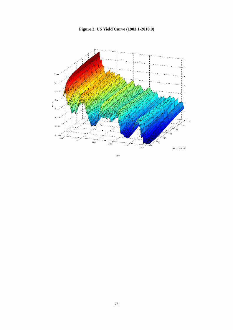
of each month to form a monthly data set for our empirical analysis. Figure 3 shows the

yield curve dynamics of the data set.

[Figure 3. US Yield Curve (1983.1-2010.9)]

For macroeconomic variables, we choose the monthly CPI annual inflation rate as an

exogenous variable in determining the factor dynamics of the LARX model. Inflation is not

only important for determining the level of interest rates in the long run, as described by

5

Fisher’s equation, but is also highly correlated with interest rates as can be seen from Figure

2. Although it is interesting to explore the joint dynamics of the yield curve and inflation,

as our primary goal is to forecast the yield curve, we opt for the simple and effective method

of taking inflation as an exogenous variable in the state dynamics. It is also beneficial and

possible to include other macroeconomic variables or factors in the states. We relegate this

investigative task to future work regarding defining the optimal set of variables or factors

to be included. Our focus remains using inflation as a relevant macroeconomic variable to

illustrate the effectiveness of the ADNS model.

3 Adaptive dynamic Nelson-Siegel model

In the adaptive dynamic Nelson-Siegel (ADNS) model, the cross section of the yield curve

is assumed to follow the Nelson and Siegel (1987) framework, based on which three factors

are extracted via the ordinary least squares (OLS) method. For each single factor, a local

autoregressive model with exogenous variables (LARX) is employed to forecast. In the

LARX approach, the parameters are time dependent, but each LARX model is estimated

at a specific point of time under Local Homogeneity. Local homogeneity means that, for any

particular time point, there exists a past subsample over which the parameters, though time

varying, are approximately constant. In this situtation the time-varying model does not

deviate much from the stationary model with constant parameters over the subsample, and

hence the local maximum likelihood estimator is still valid. The interval of local homogeneity

is automatically selected for each time point by sequentially testing the significance of the

divergence.

3.1 Extract Nelson-Siegel factors

In the framework of Nelson and Siegel (1987), the yield curve can be formulated as follows:

yt(τ) = β1t + β2t

(1− e−λτ

λτ

)+ β3t

(1− e−λτ

λτ− e−λτ

)+ εt(τ), εt(τ) ∼ N(0, σ2

ε ) (1)

where yt(τ) denotes the yield curve with maturity τ (in months) at time t. Parameter λ

controls the exponentially decaying rate of the loadings for the slope and curvature factors,

and a smaller value produces a slower decay. However, within a wide range of values, Nelson

and Siegel (1987) find that the goodness-of-fit of the yield curve is not very sensitive to the

specific value of λ. In our study, we follow Diebold and Li (2006) and set λ = 0.0609 which

maximizes the curvature loading at a medium maturity of 30 months. Under fixed λ, if there

exists any form of non-stationarity in the observations yt(τ), then it is solely attributed to

changes in the sequences of the factors.

6

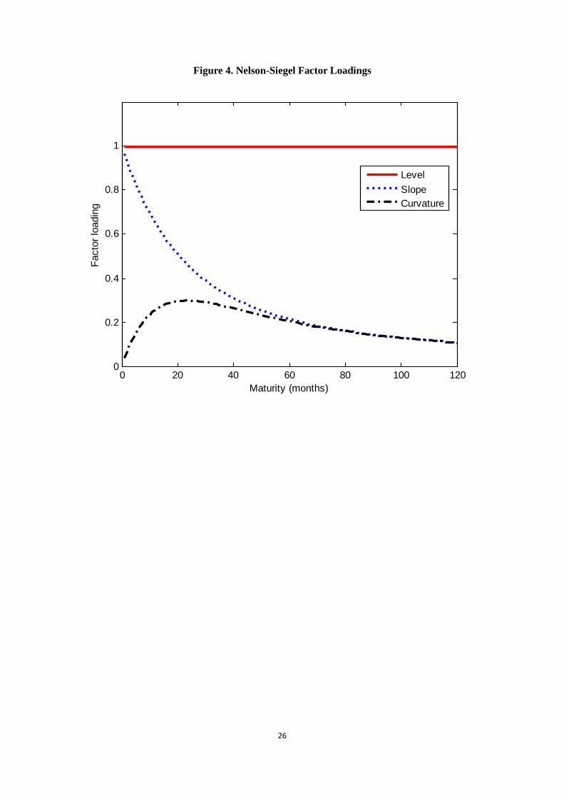
The three factors, β1t, β2t and β3t are denoted as level, slope and curvature, respectively.

Their loadings on the yield curve are displayed in Figure 4. The loadings of β1t are 1 for

all maturities, implying that the higher the factor, the higher the level of the whole yield

curve. Empirically it is close to the long-term yield of 10 years. The loadings of β2t start

from 1 at the instantaneous spot rate and decay towards zero as maturities increase. The

average value of β2t is negative, indicating a normal upward-sloping yield curve; when β2t is

positive, it leads to a downward slope of the yield curve which often anticipates recessions.

The slope factor, β2t, is highly correlated with the negative spread of the yield curve, e.g.,

the difference between the short-term and long-term yields, −[y(120)− y(3)]. The loadings

of β3t display a humped shape, which peak around the maturities of medium duration.

Thus β3t is named a curvature factor. A positive value of β3t indicates that the yield curve

is concave with a hump, while a negative value means that the yield curve is convex with

an inverted hump. Empirically, it is approximated by twice the medium yield minus the

sum of short- and long-term yields, e.g., 2× y(24)− [y(120) + y(3)].

[Figure 4. Nelson-Siegel Factor Loadings]

The time evolution of the three factors is displayed in Figure 5, where the empirical proxies

of level, slope and curvature are also depicted in dotted lines. It shows that the three factors

are consistent with the empirical proxies, demonstrating similar values and patterns. The

correlations between the three factors and their proxies are as high as 0.976, 0.991 and

0.997, respectively. The level factor has a downward trend, which indicates that the yield

curve, on average, has been decreasing along time. The slope factor is negative in most

cases, which means that the yield curve is normally upward sloping. Nevertheless, a few

positive values are observed at three locations, specifically leading the NBER recessions.

The curvature factor fluctuates wildly around zero, indicating that both the hump and

inverted hump shapes occur frequently. Nonetheless the curvature has been persistently

negative during the past decade.

[Figure 5. Time Evolution of Nelson-Siegel Factors Extracted from US Yield Curve]

3.2 Local autoregressive model with exogenous variables

Now, for each one-dimensional factor βjt, with j = 1, 2 and 3, a local model is adopted

to perform forecast. For notational simplification, we drop the subscript j in the following

elaboration. Given a univariate time series βt ∈ R, we identify a past subsample for any

7

particular time point, over which all the included observations can be well represented by

a local model with approximately constant parameters, i.e., local homogeneity holds. More

specifically, given all available past observations for the time point, we seek the longest time

interval, beyond which there is a high possibility of a structural change occurring which

means the local homogeneity assumption no longer holds. The likelihood ratio test helps

to select the local subsample. Among many possible modeling candidates, we focus on

an AR(1) model, motivated by its simplicity, parsimony and hence a good out-of-sample

forecasting ability. Moreover, to increase modeling flexibility, we allow relevant exogenous

variables in addition to the one lagged autoregressive component. The proposed model is a

local AR(1) model with exogenous variables, or a LARX(1) model.

The LARX(1) model is defined through a time-varying parameter set θt:

ft = θ0t + θ1tft−1 + θ2tXt−1 + µt, µt ∼ N(0, σ2t ) (2)

where θt = (θ0t, θ1t, θ2t, σt)>. The innovations µt have a mean of zero and a variance of σ2

t .

In our study, the three Nelson-Siegel factors are individually represented by the LARX(1)

model and share the inflation rate as the exogenous variable, X. The model parameters are

time dependent and can be obtained by the (quasi) maximum likelihood estimation, once

the local subsample is specified.

Suppose the subsample is given for time point s, denoted as Is = [s−ms, s−1], over which

the process can be safely described by an autoregressive model with exogenous variables

(ARX) with constant parameter θs. Then suppose that the local maximum likelihood

estimator θs is defined as:

θs = arg maxθ∈Θ

L(f ; Is, θ,X)

= arg maxθ∈Θ

{−(ms − 1) log σs −

1

2σ2s

s−1∑t=s−ms+1

(ft − θ0 − θ1ft−1 − θ2Xt−1)2

}

where Θ is the parameter space and L(f ; Is, θ,X) is the local log-likelihood function. In

practice, the stable subsample is unknown and the number of possible candidates is large,

e.g. as many subsamples as there are sample periods. Our goal is to select an optimal

subsample among a finite set of alternatives. The finest search would be on all possible

candidates contained in the sample. However, to alleviate the computational burden, we

divide the sample into discrete intervals with each interval containing M periods, such that

the resulting number of subsamples, Ks, is roughly the available sample length divided by

M . Suppose there are Ks candidate subsamples for any particular time point s, or

I(1)s , · · · , I(Ks)

s with I(1)s ⊂ · · · ⊂ I(Ks)

s ,

8

which starts from a short subsample, I(1)s , where the ARX(1) model with constant pa-

rameters provides a reasonable fit. The selection procedure then iteratively extends this

subsample with the next interval of M periods and sequentially tests for possible structural

change in the next longer subsample. This is performed via an `− 1 type of likelihood ratio

test. The test statistic is defined as

T (k)s =

∣∣L(I(k)s , θ(k)

s )− L(I(k)s , θ(k−1)

s )∣∣1/2,

where L(I(k)s , θ

(k)s ) = maxθ∈Θ L(f ; I

(k)s , θ,X) denotes the fitted likelihood under hypotheti-

cal homogeneity and L(I(k)s , θ

(k−1)s ) = L(f ; I

(k)s , θ

(k−1)s , X) refers to the likelihood with the

estimate under accepted local homogeneity in the testing subsample. The test statistic mea-

sures the difference between these two estimates. If the difference is significant, it indicates

that the model changes more than what would be expected due to sampling changes. If this

is the case, then the procedure terminates and the latest accepted subsample is selected.

Otherwise, we accept the longer subsample and continue the procedure until a change is

found or the longest subsample, I(Ks)s , is reached under local homogeneity. The significance

level is controlled by critical values obtained by Monte Carlo simulations. The basic idea is

to generate a stationary ARX(1) time series based on the available data, i.e., where local

homogeneity is guaranteed, and then compute the cut-off value that leads to a decision

of not rejecting the null hypothesis of homogeneity. The cut-off values tend to be critical

values. The details of the computation of the critical values can be found in Chen et al.

(2010).

The local model is then fitted over the selected subsample and can be safely used for

predictions. Since the selection of subsamples is time dependent, the optimal subsamples

are changing over time. A related assumption is that the selected model holds with high

probability for the forecast horizon. We may wish to predict structural change out of sample,

such as Pesaran, Pettenuzzo and Timmermann (2006) who use a Bayesian procedure to

incorporate the future possibility of breaks. In this regard, our approach is less sophisticated,

however it is less computationally demanding and, as will be shown in the results, is very

effective.

3.3 Modeling, forecasting factors and the yield curve

Essentially, the ADNS model can be summarized in a state-space representation as follows:

yt(τ) = β1t + β2t

(1− e−λτ

λτ

)+ β3t

(1− e−λτ

λτ− e−λτ

)+ εt(τ) (3)

βit = θ(i)0t + θ

(i)1t βit−1 + θ

(i)2t Xt−1 + v

(i)t , v

(i)t ∼ (0, σ2

it), i = 1, 2, 3. (4)

9

At each point of time, once the most recent optimal subsample is selected, the resulting

model amounts to a DNS model with possible exogenous factors. This is in spite of our

ADNS model taking time-varying coefficients. However, we will show that, with adaptive

selection of subsample length, the forecast accuracy is substantially improved.

We estimate two specifications of the ADNS model. One is denoted as LAR and has no

exogenous factor, and the other denoted as LARX and has an exogenous factor, i.e., CPI

inflation. The LAR specification provides a pure comparison to the DNS model with an

AR(1) process for each factor, and shows the stark difference in forecasts resulting from

the adaptive feature. The LARX specification then shows additional benefits gained by

including inflation.

The yield curve forecast h-step ahead is directly based on the h-step ahead forecast of

Nelson-Siegel factors:

yt+h/t(τ) = β1,t+h/t + β2,t+h/t

(1− e−λτ

λτ

)+ β3,t+h/t

(1− e−λτ

λτ− e−λτ

)(5)

where, for the LAR specification, the factor forecasts are obtained by

βi,t+h/t = θ0t + θ1tβi,t, i = 1, 2, 3, (6)

and, for the LARX specification, by

βi,t+h/t = θ0t + θ1tβi,t + θ2tXt, i = 1, 2, 3. (7)

The coefficient θjt (j = 0, 1, 2) is obtained by regressing βi,t on an intercept and βi,t−h for

LAR, and by regressing βi,t on an intercept, βi,t−h and Xt−h for LARX. We follow Diebold

and Li (2006) to directly predict factors at t+h with factors at time t, instead of using the

iterated one-step ahead forecast, to obtain a multistep ahead forecast.

4 Empirical application of the ADNS model

In this section, we apply the ADNS model to perform out-of-sample forecast of the yield

curve and elaborate on its usefulness in detecting structural breaks and monitoring param-

eter changes in the state dynamics.

4.1 Out-of-sample forecast performance of ADNS

Diebold and Li (2006) show that the DNS model does well for out-of-sample forecasts in

comparison with various other popular models. So, compared with the DNS model, how

much can the ADNS model benefit from this adaptive feature for forecasting yields? We

10

perform an out-of-sample forecast comparison to answer this question.

4.1.1 Forecast procedure

We report the factor and yield curve forecasts of the ADNS model with the two specifica-

tions: LARX(1) and LAR(1).

We use the yield data as described in Section 2 from 1983:1 to 2010:9. We make an out-

of-sample forecast in real time starting the estimation from 1997:12, and make 1-month,

3-months, 6-months and 12-months ahead forecasts for 1998:1, 1998:3, 1998:6 and 1998:12,

respectively. We move forward one period at a time to redo the estimation and forecast

until reaching the end of the sample. The 1-month forecast is made for 1998:1 to 2010:9,

a total of 153 months; the 3-, 6- and 12-months ahead forecasts are made for 1998:3 to

2010:9 with 151 months, 1998:6 to 2010:9 with 148 months, and 1998:12 to 2010:9 with 142

months, respectively.

At each point of estimation, we use data up to that point. We first extract the three

Nelson-Siegel factors using OLS for the available sample. For each factor, we assume an

LAR(1) or LARX(1) process for the different forecast horizons, and test the stability back-

ward using our method as described in the previous section. To reduce computational

burden, we use a universal set of intervals for each time point, starting with the shortest

subsample covering the past 6 months, with the interval between two adjacent subsamples

equal to 6 months, ending with the longest subsample. Once an optimal subsample is se-

lected against the next longer subsample, the change is understood as having taken place in

the 6 month’ period in between. In doing so, we trade off precision in break identification

with computational efficiency. However, since our primary goal is to estimate from the

identified sample with relatively constant parameters, the lack of a few observations are

not of major concern. Also, as many changes can happen smoothly, point identification of

breaks may not be precise.

We choose the most recent stable subsample as the optimal sample to estimate the pa-

rameters, based on which we do out-of-sample forecasts 1-, 3-, 6- to 12- months ahead

as in Equation (6) for LAR and in Equation (7) for LARX, respectively. The predicted

Nelson-Siegel factors at the specific horizon will then be used to form a yield forecast as in

Equation (5).

4.1.2 Alternative models for comparison

For comparison, we choose the DNS model and the random walk model. The DNS model

is a direct and effective comparison for our ADNS model. The random walk model serves

as a very natural and popular benchmark for financial time series with non-stationary

characteristics.

11

1) DNS model

We forecast the Nelson-Siegel factors and yield curve with the DNS model using three

strategies of sample length selection: a five-year rolling estimation, a ten-year rolling es-

timation and a recursive estimation. With a rolling estimation, we fix the sample length

at each point of time. For the five-year or ten-year rolling estimation, we include in the

regression the most recent 60 or 120 months’ observations, respectively. With the recursive

estimation, we expand the sample length one point at a time as we move forward, with

the initial sample being about 15 years (180 months). These three cases correspond to a

comparison with increasing sample lengths.

These rolling and recursive strategies are popular in forecast practice. The recursive

estimation aims to increase information efficiency by extending the available sample as

much as possible, such as that used in Diebold and Li (2006) with an initial sample length

of about 9 years and extending it forward. The rolling estimation reflects the idea of making

a trade-off between information efficiency and possible breaks in the data generating process,

such as in the 15-year rolling window used in Favero, Niu and Sala (2012). Note that a

predetermined sample length is unable to simultaneously serve both purposes: ensure stable

estimation under stationarity and have a quick reaction to structural changes.

The forecast of factors and yields are similar to the ADNS model with the selected

sample length, as shown in Equations (5) and (6). The only difference is that parameters

θj (j = 0, 1, 2) are obtained by regressing βi,t on an intercept and βi,t−h with a sample of

predetermined length.

2) Random walk model

With the random walk model of no drift, yields are directly forecasted by its current

value, or

yt+h/t(τ) = yt(τ).

4.1.3 Measures of forecast comparison

We use two measures as indicators of forecast performance, the forecast root mean squared

error (RMSE) and the mean absolute error (MAE). We calculate these measures for the

Nelson-Siegel factors and yields in the DNS model, and for yields in the random walk model.

4.1.4 Forecast results

Table 1 reports the forecast RMSE and MAE for the three Nelson-Siegel factors for the

forecast horizons (denoted by h) of 1, 3, 6 and 12 months, respectively. Each column

reports the results of the ADNS model with the two specifications of LARX and LAR,

and of the DNS models using three different sample length strategies: 5-year and 10-year

12

rolling window with fixed lengths and the recursive forecast with expanding window length.

In each column, the number in bold indicates the best forecast for each horizon and each

measure, and the underlined number the second best.

[Table 1. Forecast Comparison of Factors]

Table 1 shows that, without exception, the LAR and LARX specifications are always

the best two across all factors, horizons and RMSE/MAE measures. The ADNS model,

with the adaptive selection of sample lengths, always forecasts better than the DNS model

with various predetermined window lengths. The advantage grows as the forecast horizon

increases. At the 12-month forecast horizon, the RMSE/MAE of the ADNS are, in general,

40-50 percent less than those produced by the DNS models. The LARX model tends to

outperform the LAR model, indicating that the inflation factor helps to predict the yield

factors in the ADNS model, in addition to their lagged information.

Among the DNS models, there is no clear pattern as to which window length performs the

best. Although in most cases the 10-year rolling window produces better forecasts than the

5-year rolling window, the recursive window, which incorporates more observations, tends

to do better for the first two factors but fare worse for the third factor than the 10-year

rolling window.

To visualize the forecast differences, we plot the factor forecasts from the LARX of the

ADNS model and the 10-year rolling window of the DNS model together with the real data

in Figure 6. Each row displays the forecast for one factor, for the forecast horizons of 1-,

6- and 12 months, respectively. Factors extracted from real yields are displayed with solid

lines; LARX forecasts of the ADNS are displayed with dotted lines, and the 10-year rolling

forecasts of the DNS with dashed lines. Although it is difficult to distinguish the three

series for the 1-month ahead forecast because they are so close to each other, as the forecast

horizon lengthens, it is clear that the dotted line of the LARX forecast tends to trace the

factor dynamics much more closely than does the DNS. What is dramatic is its capability of

predicting the large swings of slope and curvature during the financial crisis. From 2007 to

2008, the slope reduced sharply reflecting an ever decreasing short rate, while initially the

LARX reacts insufficiently to the decline in the 6- and 12-month ahead forecast, it quickly

catches up and correctly predicts the sharp fall during 2008. The DNS with the 10-year

rolling window, however, not only reacts with a persistent lag, but also wrongly predicts

the change in direction for a persistent period.

[Figure 6. Plots of Factor Forecasts with LARX of ADNS and 10-year Rolling of DNS]

13

Table 2 reports the forecast RMSE and MAE for yields with the selected maturities of 3

months, 1 year, 3 years, 5 years and 10 years. In addition to the forecasts from the ADNS

and the DNS models, we also report the random walk forecast.

[Table 2. Forecast Comparison of Yields]

Again, the ADNS model dominates the DNS model across yields, forecast horizons and

forecast measures. Even if we compare the second best result of the ADNS model and the

best result among the DNS models, the reduction in the RMSE/MAE of the ADNS model

reaches about 30 percent for the 3-month ahead forecast, and even to about 60 percent for

the 12-month ahead forecast. The advantage is tremendous! Compared with the random

walk model, the ADNS model does not always have an absolute advantage, for the short-

to-medium yields at the 1-month ahead forecast. The outperformance begins to be obvious

from the 3-month ahead forecast. Also, the reduction in RMSE/MAE when compared with

the random walk is fairly substantial ranging between 30 to 60 percent in multistep ahead

forecasts.

In Figure 7 we plot the yield forecast from the LARX of the ADNS model and the 10-

year rolling window of the DNS model together with the real data. We select yields with

maturities of 3 months, 36 months and 120 months to represent the short-, medium- and

long-term yields. Each row displays the forecast for one yield, for the forecast horizons of

1, 6 and 12 months, respectively. Real yields are displayed by solid lines; LARX forecasts

are displayed by dotted lines, and 10-year rolling forecast by dashed lines. As the forecast

horizon lengthens, it is clear that the dotted line of the LARX forecasts tends to follow

the yield dynamics much more closely than the DNS forecasts. The excellence of LARX in

predicting dramatic changes and large swings in factors now follows through to superiority

in predicting yield changes. The ADNS model can not only accurately predict the large

swings in short- and medium-term yields, but also captures the subtle movement in the

10-year yields 6 months or even 12 months earlier.

[Figure 7. Plots of Yields Forecast with LARX and 10-year Rolling]

4.1.5 Lengths of stable subsamples

Table 3 summarizes the average lengths detected for sample stability along the forecast

for each factor and each horizon. When h = 1, it is a standard AR(1)/ARX(1) model

of lag 1. When h > 1, it is an AR(1)/ARX(1) model with lag h. The overall length of

14

the stable subsample is surprisingly low compared to the conventional sample size used

in the literature for yield curve forecasts at a monthly frequency, with a maximum of 73

months (about six years) for the first Nelson-Siegel factor and for the one-month ahead

forecast from the LAR specification. For other cases, the average lengths of the stable

subsample is around 30 months, or two-and-a-half years, which is much shorter than the

conventionally-used 5-year, 10-year rolling or recursive samples.

The dominating performance of the adaptive approach indicates that the instability prob-

lems inherent in yield factor dynamics outweighs the information inefficiency with short

samples, such that shorter samples are preferred to longer samples with more observations.

The question is how short the selected subsample should be. Instead of relying on a rule-

of-thumb selection of a predetermined window length, our approach detects the optimal

subsamples at each point of time employing the adaptive procedure.

[Table 3. Average Lengths of Stable Sample Intervals Detected by LAR and LARX]

4.2 Detecting breaks and monitoring parameter evolvement

We have shown that the ADNS model predicts yield dynamics remarkably better than the

DNS model, benefiting from the adaptive feature of the model. There must be useful infor-

mation hidden in the detected breaks and parameter evolvements that drive this excellence

in prediction. Understanding the time-varying features of the state dynamics in real time

would be very valuable not only for forecasts, but also for real-time diagnosis of the yield

curve and for policy investigation.

Figure 8 plots the detected stable subsamples and breaks along the forecasting time for

each factor. We report the results of the 1-step ahead forecast of the LARX(1) model, i.e.,

a standard AR(1) model with the most adjacent lag and lagged inflation. The vertical axis

denotes the time when the estimation or forecast is made. At each point of time, an optimal

subsample is detected which is shown as a (light yellow) line along the horizontal axis of

time. At the end of the line, a (dark blue) dotted line indicates the period, in this case six

months, during which the most recent break happens, i.e., the immediate interval beyond

the identified stable subsample. When these (dark blue) dotted lines are stacked along the

forecast time, i.e., the vertical dimension, some common areas of detected breaks become

evident.

[Figure 8. Breaks of Factors Detected in the LARX(1)]

15

Observing Figure 8, we find that the stable subsamples of the level factor are typically

longer than those of slope and curvature. For level, the intervals of 1994-1998, 1998-2003

and 2003-2008 are identified as relatively stable within the whole sample. For slope and cur-

vature, breaks are constantly detected during the forecast exercise, indicating ever-evolving

parameters. Moreover, breaks within the level factor often lead breaks within the other two

factors. There are three occasions of sequential breaks led by level breaks in 1994, 1998 and

2003, with breaks in slope and curvature following in 1995, 1998 and 2003. Overall, there

seems to be a common break in all three factors just at the beginning of the financial crisis

and recession in 2008.

Those major breaks in level align with some big events and debated policy change. For

example, the 1998 and 2008 breaks correspond well to the 1997-1998 financial market tur-

moil and the 2008 financial crisis. The break at the beginning of 2003 follows the internet

bubble bursting, and when the US Federal Reserve had begun to conduct relatively loose

monetary policy for a prolonged period. Taylor (2011), among many others, admonishes

that “interests rates were held too low for too long by the Federal Reserve”. Measured

by the Taylor rule (Taylor, 1993), the monetary reaction to inflation was remarkably low

between 2003 and 2005. Ang et al. (2011) estimate a time-varying Taylor rule using the

quadratic term structure model and confirm similar findings with richer data of the whole

yield curve. The policy change is criticized as having accommodated the financial bubble

which eventually ends in the recent financial crisis.

When breaks are detected, it is because parameters have changed so dramatically that

the most recent sample estimates are not valid when extending the sample further back.

Therefore a close monitoring of the evolvement of parameters is helpful to understand the

origins of the breaks.

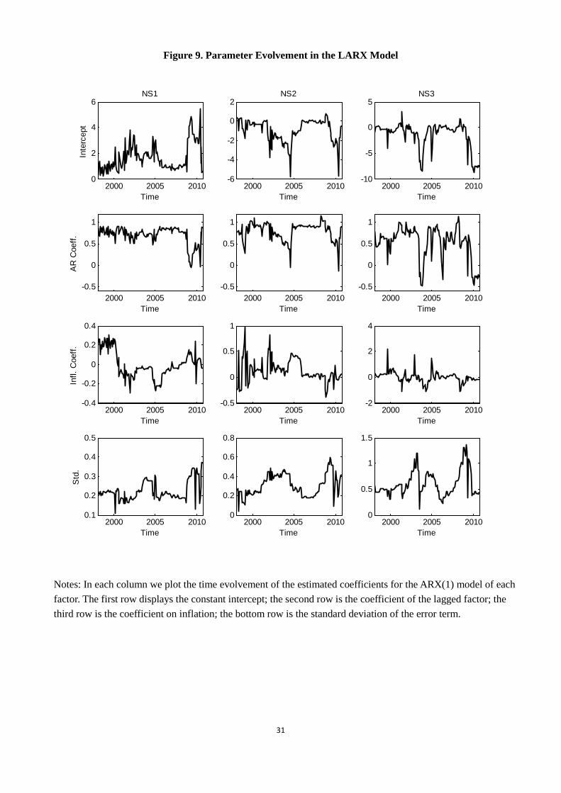
Figure 9 presents the parameter estimates along the forecasting path. For each of the

three factors, the ARX process involves four parameters as in Equation (2): the intercept,

θ0t, the autoregressive coefficient, θ1t, the coefficient of inflation, θ2t, and the standard

deviation of the error term, σt. We report in each column the evolvement of the four

parameters for each factor.

[Figure 9. Parameter Evolvement in the LARX Model]

This figure shows that the coefficients of the ARX(1) model of each Nelson-Siegel factor

vary wildly through time, which justifies the application of an adaptive approach. Within

the optimal interval detected at the each point of time, the autoregressive coefficient mostly

lies within the stable range, indicating that our short memory view, indeed, can be justified

as long as our identification procedure works reasonably well.

16

We observe that the CPI inflation coefficient on the level factor changed to become

negative after 2000, which corresponds to the loose monetary policy much criticized by

academia as having precipitated the recent financial crisis. Although our model is not as

structural as those of Taylor (2011) and Ang et al. (2011), the discovery of this simple

pattern is very revealing about an important break in the relationship between interest

rates and inflation.

Simple as it is, our results provide a vivid picture of the evolvement of the volatilities

of the three factors along time. The bottom row shows that the volatilities of all factors

have surged during the recent financial crisis; other coefficients also show dramatic changes

in this period. These results indicate both higher risks and a regime switch against the

outbreak of the financial crisis.

5 Conclusion

By optimally selecting the sample period over which parameters are approximately constant

for the factor dynamics, the adaptive dynamic Nelson-Siegel (ADNS) model we propose

produces superior forecasts of the yield curve compared with both the dynamic Nelson-

Siegel model with predetermined sample lengths and the random walk model. The ADNS

model not only improves forecast precision substantially by reducing forecast errors by

between 30 to 60 percent, but also accurately predicts the large swings in the yield curve,

six to twelve months ahead of the financial crisis. This forecasting excellence originates

from its capacity to adaptively and swiftly detect structural breaks. The detected breaks

and the evolvement of the estimated parameters are revealing about the structural changes

in economic conditions and monetary policy. We believe this model and the method used

are of great value to policy makers, practitioners and academics alike for drawing ever

more precise and timely determinations from the yield curve information about imminent

recessions.

Moreover, for monitoring and forecasting purposes, this adaptive modeling method is

data-driven and can be widely applied to other macroeconomic and financial time series,

either uni- or multivariate, stationary or nonstationary, with different sources of changes

including heteroskedasticity, structure break, and regime switching.

Acknowledgement

Linlin Niu acknowledges the support of the Natural Science Foundation of China (Grant

No. 70903053).

17

References

Ang, A. and Bekaert, G. 2002. Regime switches in interest rates, Journal of Business and

Economic Statistics 20: 163–182.

Ang, A. and Piazzesi, M. 2003. A no-arbitrage vector autoregression of term structure

dynamics with macroeconomic and latent variables, Journal of Monetary Economics

50(4): 745–787.

Ang, A., Boivin, J., Dong, S. and Loo-Kung, R. 2011. Monetary policy shifts and the term

structure, Review of Economic Studies 78: 429–457.

Bansal, R. and Zhou, H. 2002. Term structure of interest rates with regime shifts, Journal

of Finance 57(5): 1997–2043.

Chen, Y., Hardle, W. and Pigorsch, U. 2010. Localized realized volatility modelling, Journal

of the American Statistical Association 105: 1376–1393.

Diebold, F. X. and Inoue, A. 2001. Long memory and regime switching, Journal of Econo-

metrics 105: 131–159.

Diebold, F. X. and Li, C. 2006. Forecasting the term structure of government bond yields,

Journal of Econometrics 130: 337–364.

Duffee, G. R. 2002. Term premia and interest rate forecasts in affine models, Journal of

Finance 57: 405–443.

Duffee, G. R. 2011. Forecasting with the term structure: The role of no-arbitrage restric-

tions, working paper, Johns Hopkins University.

Fama, E. and Bliss, R. 1987. The information in long-maturity forward rates, American

Economic Review 77: 680–692.

Favero, C. A., Niu, L. and Sala, L. 2012. Term structure forecasting: No-arbitrage restric-

tions versus large information set., Journal of Forecasting. Forthcoming.

Granger, C. W. and Joyeux, R. 1980. An introduction to long memory time series models

and fractional differencing, Journal of Time Series Analysis 1: 5–39.

Granger, C. W. J. 1980. Long memory relationships and the aggregation of dynamic models,

Journal of Econometrics 14: 227–238.

Granger, C. W. J. and Hyung, N. 2004. Occasional structural breaks and long memory with

an application to the S&P500 absolute stock returns, Journal of Empirical Finance

11: 399–421.

18

Guidolin, M. and Timmermann, A. 2009. Forecasts of US short-term interest rates: A

flexible forecast combination approach, Journal of Econometrics 150: 297–311.

Gurkaynak, R. S., Sack, B. and Wright, J. H. 2007. The U.S. treasury yield curve: 1961 to

the present, Journal of Monetary Economics 54(8): 2291–2304.

Hosking, J. R. M. 1981. Fractional differencing, Biometrika 68: 165–176.

Mishkin, F. S. 1990. The information in the longer maturity term structure about future

inflation, The Quarterly Journal of Economics 105: 815–828.

Nelson, C. and Siegel, A. 1987. Parsimonious modeling of yield curve, Journal of Business

60: 473–489.

Pesaran, M. H., Pettenuzzo, D. and Timmermann, A. G. 2006. Forecasting time series

subject to multiple structural breaks, Review of Economic Studies 73: 1057–1084.

Taylor, J. B. 1993. Discretion versus policy rules in practice, Carnegie-Rochester Conference

Series on Public Policy 39: 195–214.

Taylor, J. B. 2011. Origins and policy implications of the crisis, in: R. Porter (Ed.), New

Directions in Financial Services Regulationk, MIT Press, Cambridge, MA, pp. 13–22.

19

20

Table 1. Forecast Comparison of Factors

NS1 h = 1 h = 3 h = 6 h = 12

RMSE MAE RMSE MAE RMSE MAE RMSE MAE

LARX 0.281 0.204 0.334 0.247 0.374 0.273 0.462 0.342

LAR 0.307 0.216 0.364 0.266 0.430 0.338 0.453 0.344

5-year Rolling 0.333 0.239 0.462 0.356 0.623 0.496 0.738 0.540

10-year Rolling 0.330 0.232 0.463 0.350 0.617 0.495 0.780 0.622

Recursive 0.331 0.232 0.461 0.346 0.610 0.490 0.729 0.559

NS2 h = 1 h = 3 h = 6 h = 12

RMSE MAE RMSE MAE RMSE MAE RMSE MAE

LARX 0.381 0.278 0.530 0.414 0.704 0.495 0.873 0.620

LAR 0.399 0.291 0.568 0.426 0.726 0.552 1.024 0.698

5-year Rolling 0.453 0.343 0.893 0.714 1.570 1. 922 3.026 2.568

10-year Rolling 0.434 0.321 0.782 0.599 1.234 1.025 1.889 1.619

Recursive 0.431 0.320 0.772 0.600 1.203 1.013 1.853 1.601

NS3 h = 1 h = 3 h = 6 h = 12

RMSE MAE RMSE MAE RMSE MAE RMSE MAE

LARX 0.722 0.518 1.017 0.750 1.179 0.860 1.124 0.858

LAR 0.777 0.550 1.103 0.809 1.292 0.945 1.299 0.989

5-year Rolling 0.889 0.665 1.497 1.125 2. 171 1.693 3.204 2. 683

10-year Rolling 0.863 0.644 1.394 1.039 1.913 1.496 2.529 2.085

Recursive 0.868 0.647 1.442 1.075 1.992 1.537 2.660 2.206

Notes for Table 1 and 2: 1) The 1-month ahead forecast period is 1998:1 to 2010:9, a total of 153 months. The 3-month

ahead forecast period is 1998:3-2010:9 with 151 months. The 6-month ahead forecast period is 1998:6-2010:9 with 148 months and the 12-month ahead forecast period is 1998:12-2010:9 with 142 months.

2) For each column, the best forecast, i.e., smallest RMSE or MAE, is marked in bold-face; the second best is underlined.

21

Table 2. Forecast Comparison of Yields

y(3) h = 1 h = 3 h = 6 h = 12

RMSE MAE RMSE MAE RMSE MAE RMSE MAE

LARX 0.331 0.231 0.429 0.316 0.612 0.408 0.662 0.452

LAR 0.297 0.199 0.436 0.309 0.589 0.427 0.771 0.514

5-year Rolling 0.346 0.237 0.722 0.529 1.345 1.066 2.871 2.339

10-year Rolling 0.326 0.219 0.637 0.447 1.077 0.860 1.814 1.568

Recursive 0.318 0.208 0.626 0.460 1.048 0.878 1.778 1.577

Random Walk 0.254 0.153 0.547 0.363 0.927 0.673 1.650 1.306

y(12) h = 1 h = 3 h = 6 h = 12

RMSE MAE RMSE MAE RMSE MAE RMSE MAE

LARX 0.259 0.196 0.392 0.296 0.576 0.397 0.602 0.460

LAR 0.244 0.176 0.408 0.293 0.551 0.412 0.685 0.523

5-year Rolling 0.280 0.216 0.675 0.508 1.264 1.020 2.608 2.150

10-year Rolling 0.260 0.197 0.601 0.458 1.024 0.833 1.722 1.511

Recursive 0.269 0.206 0.622 0.498 1.042 0.884 1.732 1.544

Random Walk 0.251 0.176 0.561 0.401 0.927 0.699 1.582 1.284

y(36) h = 1 h = 3 h = 6 h = 12

RMSE MAE RMSE MAE RMSE MAE RMSE MAE

LARX 0.296 0.229 0.434 0.331 0.542 0.420 0.494 0.378

LAR 0.300 0.211 0.463 0.348 0.533 0.405 0.532 0.413

5-year Rolling 0.330 0.256 0.640 0.497 1.045 0.802 1.954 1.559

10-year Rolling 0.326 0.253 0.627 0.478 0.955 0.754 1.478 1.234

Recursive 0.330 0.256 0.650 0.507 0.981 0.781 1.486 1.260

Random Walk 0.300 0.228 0.573 0.448 0.845 0.679 1.237 1.026

y(60) h = 1 h = 3 h = 6 h = 12

RMSE MAE RMSE MAE RMSE MAE RMSE MAE

LARX 0.298 0.230 0.414 0.322 0.486 0.382 0.459 0.360

LAR 0.309 0.228 0.442 0.341 0.497 0.393 0.469 0.378

5-year Rolling 0.335 0.259 0.575 0.453 0.873 0.673 1.487 1.166

10-year Rolling 0.340 0.265 0.592 0.459 0.859 0.680 1.258 1.063

Recursive 0.342 0.266 0.608 0.471 0.878 0.694 1.252 1.044

Random Walk 0.301 0.231 0.532 0.429 0.753 0.607 1.005 0.829

y(120) h = 1 h = 3 h = 6 h = 12

RMSE MAE RMSE MAE RMSE MAE RMSE MAE

LARX 0.276 0.219 0.343 0.269 0.387 0.304 0.425 0.330

LAR 0.284 0.217 0.363 0.281 0.404 0.329 0.403 0.322

5-year Rolling 0.295 0.230 0.427 0.354 0.587 0.481 0.822 0.656

10-year Rolling 0.290 0.221 0.437 0.354 0.601 0.472 0.828 0.692

Recursive 0.299 0.226 0.452 0.365 0.622 0.494 0.818 0.664

Random Walk 0.287 0.213 0.443 0.355 0.595 0.485 0.718 0.566

22

Table 3. Average Lengths of Stable Sample Intervals Detected by LAR and LARX (Unit: month)

NS factor h = 1 h = 3 h = 6 h = 12

LAR LARX LAR LARX LAR LARX LAR LARX

NS1 73 43 29 31 33 33 37 40 NS2 34 31 25 28 28 30 31 31

NS3 28 28 26 27 27 28 31 29

23

Figure 1. Time Plot of the NS Level Factor and its Sample Autocorrelation Function

1985 1990 1995 2000 2005 2010

4

5

6

7

8

9

10

11

12

13%

NS1 - Level

NS 1st factor10 year yield

24

Figure 2. Three Yields and CPI Inflation in the US (1983.1-2010.9)

25

Figure 3. US Yield Curve (1983.1-2010.9)

26

Figure 4. Nelson-Siegel Factor Loadings

0 20 40 60 80 100 1200

0.2

0.4

0.6

0.8

1

Maturity (months)

Fact

or lo

adin

g

LevelSlopeCurvature

27

Figure 5. Time Evolution of Nelson-Siegel Factors Extracted from US Yield Curve (1983.1-2010.9)

1985 1990 1995 2000 2005 2010

4

6

8

10

12

Time

%

NS1 - Level

NS 1st factor10 year yield

1985 1990 1995 2000 2005 2010-6

-5

-4

-3

-2

-1

0

1

Time

%

NS2 - Slope

NS 2nd factor- (10 year - 3 month)

1985 1990 1995 2000 2005 2010-8

-6

-4

-2

0

2

4

Time

%

NS3 - Curvature

NS 3rd factor2*2 year - (10 year + 3 month)

28

Figure 6. Plots of Factor Forecasts with LARX and 10-year Rolling

2000 2002 2004 2006 2008 20103.5

4

4.5

5

5.5

6

6.5

7NS1, h = 1

%

Time2000 2002 2004 2006 2008 2010

3.5

4

4.5

5

5.5

6

6.5

7NS1, h = 6

%

Time2000 2002 2004 2006 2008 2010

3.5

4

4.5

5

5.5

6

6.5

7NS1, h = 12

%

Time

2000 2002 2004 2006 2008 2010-6

-5

-4

-3

-2

-1

0

1NS2, h = 1

%

Time2000 2002 2004 2006 2008 2010

-6

-4

-2

0

2NS2, h = 6

%Time

2000 2002 2004 2006 2008 2010-6

-5

-4

-3

-2

-1

0

1NS2, h = 12

%

Time

2000 2002 2004 2006 2008 2010-8

-6

-4

-2

0

2

4NS3, h = 1

%

2000 2002 2004 2006 2008 2010-8

-6

-4

-2

0

2

4NS3, h = 6

%

Time2000 2002 2004 2006 2008 2010

-10

-8

-6

-4

-2

0

2

4NS3, h = 12

%

Time

Note: Factors extracted from real yields are displayed by solid lines; LARX forecasts are displayed by dotted lines, and the 10-year rolling forecasts dashed lines.

29

Figure 7. Plots of Yield Forecasts with LARX and 10-year Rolling

2000 2002 2004 2006 2008 2010-2

0

2

4

6

8y(3), h = 1

%

Time2000 2002 2004 2006 2008 2010

-2

0

2

4

6

8y(3), h = 6

%

Time2000 2002 2004 2006 2008 2010

-2

0

2

4

6

8y(3), h = 12

%

Time

2000 2002 2004 2006 2008 20100

1

2

3

4

5

6

7y(36), h = 1

%

Time2000 2002 2004 2006 2008 2010

0

1

2

3

4

5

6

7y(36), h = 6

%Time

2000 2002 2004 2006 2008 20100

1

2

3

4

5

6

7y(36), h = 12

%

Time

2000 2002 2004 2006 2008 20102

3

4

5

6

7y(120), h = 1

%

Time2000 2002 2004 2006 2008 2010

2

3

4

5

6

7y(120), h = 6

%

Time2000 2002 2004 2006 2008 2010

2

3

4

5

6

7y(120), h = 12

%

Time

Note: Factors extracted from real yields are displayed by solid lines; LARX forecasts are displayed by dotted lines, and the 10-year rolling forecasts dashed lines.

30

Figure 8. Breaks of Factors Detected in the LARX(1) Model

1992 1994 1996 1998 2000 2002 2004 2006 2008 20101998

2000

2002

2004

2006

2008

2010

NS1Fo

reca

st T

ime

Time

1992 1994 1996 1998 2000 2002 2004 2006 2008 20101998

2000

2002

2004

2006

2008

2010

NS2

Fore

cast

Tim

e

Time

1992 1994 1996 1998 2000 2002 2004 2006 2008 20101998

2000

2002

2004

2006

2008

2010

NS3

Fore

cast

Tim

e

Time

Notes: The vertical axis marks the time when the estimation is made. The selected stable sample interval is marked horizontally as a light yellow line. The dark blue line marks the interval during which the most recent break is detected.

31

Figure 9. Parameter Evolvement in the LARX Model

2000 2005 20100

2

4

6NS1

Inte

rcep

t

Time2000 2005 2010

-6

-4

-2

0

2NS2

Time2000 2005 2010

-10

-5

0

5NS3

Time

2000 2005 2010-0.5

0

0.5

1

AR

Coe

ff.

Time2000 2005 2010

-0.5

0

0.5

1

Time2000 2005 2010

-0.5

0

0.5

1

Time

2000 2005 2010-0.4

-0.2

0

0.2

0.4

Infl.

Coe

ff.

Time2000 2005 2010

-0.5

0

0.5

1

Time2000 2005 2010

-2

0

2

4

Time

2000 2005 20100.1

0.2

0.3

0.4

0.5

Std

.

Time2000 2005 2010

0

0.2

0.4

0.6

0.8

Time2000 2005 2010

0

0.5

1

1.5

Time

Notes: In each column we plot the time evolvement of the estimated coefficients for the ARX(1) model of each factor. The first row displays the constant intercept; the second row is the coefficient of the lagged factor; the third row is the coefficient on inflation; the bottom row is the standard deviation of the error term.