
Accurate and Efficient Evaluation of the Second … of Tables 4.1 Tabulated data for the classical...
71
Accurate and Efficient Evaluation of the Second Virial Coefficient Using Practical Intermolecular Potentials for Gases by Maciej K. Hryniewicki A thesis submitted in conformity with the requirements for the degree of Masters of Applied Science Graduate Department of Aerospace Engineering University of Toronto Copyright c 2011 by Maciej K. Hryniewicki
Transcript of Accurate and Efficient Evaluation of the Second … of Tables 4.1 Tabulated data for the classical...

Accurate and Efficient Evaluation of the SecondVirial Coefficient Using Practical
Intermolecular Potentials for Gases
by
Maciej K. Hryniewicki
A thesis submitted in conformity with the requirements
for the degree of Masters of Applied Science
Graduate Department of Aerospace Engineering
University of Toronto
Copyright c© 2011 by Maciej K. Hryniewicki

Abstract
Accurate and Efficient Evaluation of the Second Virial
Coefficient Using Practical Intermolecular Potentials for Gases
Maciej K. Hryniewicki
Masters of Applied Science
Graduate Department of Aerospace Engineering
University of Toronto
2011
The virial equation of state p = ρRT[
1 + B(T ) ρ + C(T ) ρ2 + · · ·]
for high pressure and den-
sity gases is used for computing chemical equilibrium properties and mixture compositions of
strong shock and detonation waves. The second and third temperature-dependent virial coeffi-
cients B(T ) and C(T ) are included in tabular form in computer codes, and they are evaluated
by polynomial interpolation. A very accurate numerical integration method is presented for
computing B(T ) and its derivatives for tables, and a sophisticated method is introduced for
interpolating B(T ) more accurately and efficiently than previously possible. Tabulated B(T )
values are non-uniformly distributed using an adaptive grid, to minimize the size and storage of
the tables and to control the maximum relative error of interpolated values. The methods intro-
duced for evaluating B(T ) apply equally well to the intermolecular potentials of Lennard-Jones
in 1924, Buckingham and Corner in 1947, and Rice and Hirschfelder in 1954.
ii

Acknowledgements
I would like to thank my supervisor, Professor James J. Gottlieb, for all of his guidance and
support throughout the duration of this thesis. His enthusiasm, care and insight are much
appreciated.
I would like to acknowledge the research stipend provided by the University of Toronto
Institute for Aerospace Studies during my studies.
Finally, I would like to thank my parents, Waldemar and Izabela, and my sister, Magdalena,
for their ongoing love and encouragement. They have instilled in me the importance of educa-
tion, and I am forever grateful to them for supporting my desire to further my education in the
field of aerospace science and engineering.
Maciej K. Hryniewicki
University of Toronto Institute for Aerospace Studies
February 2011
iii

Contents
Abstract ii
Acknowledgements iii
Contents v
List of Tables vi
List of Figures viii
1 Introduction 1
2 The Virial Equation of State 4
2.1 Equations of State . . . . . . . . . . . . . . . . . . . . . . . . . . . . . . . . . . . 4
2.2 Second Virial Coefficient B(T) . . . . . . . . . . . . . . . . . . . . . . . . . . . . 6
2.3 Intermolecular Potentials . . . . . . . . . . . . . . . . . . . . . . . . . . . . . . . 7
3 Solution Methodology for B(T) and its Derivatives 15
3.1 Non-Dimensionalization of B(T) . . . . . . . . . . . . . . . . . . . . . . . . . . . 15
3.2 Derivatives of B∗(T∗) . . . . . . . . . . . . . . . . . . . . . . . . . . . . . . . . . . 16
3.2.1 Derivatives of the Classical Second Virial Coefficient Bc(T∗) . . . . . . . . 16
iv
3.2.2 Derivatives of the Quantum Correction Bq(T∗) . . . . . . . . . . . . . . . 17
3.3 Transformation for Improper to Proper Integrals . . . . . . . . . . . . . . . . . . 18
3.4 Method of Integration . . . . . . . . . . . . . . . . . . . . . . . . . . . . . . . . . 19
3.5 Method of Interpolation for Tabulated Virial Coefficients . . . . . . . . . . . . . 21
3.6 Plots of the Integrands of B∗(T∗) and its Derivatives . . . . . . . . . . . . . . . . 24
4 Results for B∗(T∗) and its Derivatives 33
4.1 Numerical Solutions for B∗(T∗) . . . . . . . . . . . . . . . . . . . . . . . . . . . . 33
4.1.1 Classical Second Virial Coefficient Bc(T∗) . . . . . . . . . . . . . . . . . . 34
4.1.2 Quantum Correction Bq(T∗) . . . . . . . . . . . . . . . . . . . . . . . . . 38
4.1.3 Selected Tabulated Solutions for B∗(T∗) . . . . . . . . . . . . . . . . . . . 42
4.2 Quantum Correction to B∗(T∗) for H2 and N2 . . . . . . . . . . . . . . . . . . . . 49
5 Concluding Remarks 51
References 56
A Assessment of New Interpolation Method 57
v

List of Tables
4.1 Tabulated data for the classical second virial coefficient and its first four deriva-
tives, using the Lennard-Jones 6-12 model, interpolated using a nonic interpolant
(m = 9). . . . . . . . . . . . . . . . . . . . . . . . . . . . . . . . . . . . . . . . . . 43
4.2 Tabulated data for the classical second virial coefficient and its first four deriva-
tives, using the Buckingham and Corner modified Buckingham model (α = 13.5
and β = 0.0), interpolated using a nonic interpolant (m = 9). . . . . . . . . . . . 44
4.3 Tabulated data for the classical second virial coefficient and its first four deriva-
tives, using the Rice and Hirschfelder modified Buckingham (exponential-six)
model (α = 13.5 and β = 0.0), interpolated using a nonic interpolant (m = 9). . . 45
4.4 Tabulated data for the quantum correction to the second virial coefficient and
its first four derivatives, using the Lennard-Jones 6-12 model, interpolated using
a nonic interpolant (m = 9). . . . . . . . . . . . . . . . . . . . . . . . . . . . . . . 46
4.5 Tabulated data for the quantum correction to the second virial coefficient and its
first four derivatives, using the Buckingham and Corner modified Buckingham
model (α = 13.5 and β = 0.0), interpolated using a nonic interpolant (m = 9). . . 47
4.6 Tabulated data for the quantum correction to the second virial coefficient and
its first four derivatives, using the Rice and Hirschfelder modified Buckingham
(exponential-six) model (α = 13.5 and β = 0.0), interpolated using a nonic
interpolant (m = 9). . . . . . . . . . . . . . . . . . . . . . . . . . . . . . . . . . . 48
A.1 Numbers of nodes and tabulated data required for interpolation of tabulated
data by various polynomial interpolation methods of different degrees (m). . . . 59
vi

List of Figures
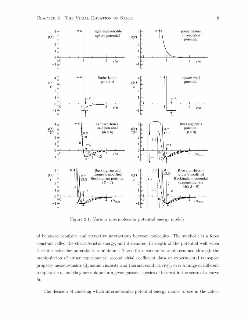
2.1 Various intermolecular potential energy models. . . . . . . . . . . . . . . . . . . . 8
3.1 Pascal’s triangle. . . . . . . . . . . . . . . . . . . . . . . . . . . . . . . . . . . . . 23
3.2 Integrands of Bc(T∗) and its first three derivatives with T∗ = 1.0. . . . . . . . . . 27
3.3 Integrands of Bc(T∗) and its first three derivatives with T∗ = 10.0. . . . . . . . . 28
3.4 Integrands of Bc(T∗) and its first three derivatives with T∗ = 100.0. . . . . . . . . 29
3.5 Integrands of Bq(T∗) and its first three derivatives with T∗ = 1.0. . . . . . . . . . 30
3.6 Integrands of Bq(T∗) and its first three derivatives with T∗ = 10.0. . . . . . . . . 31
3.7 Integrands of Bq(T∗) and its first three derivatives with T∗ = 100.0. . . . . . . . . 32
4.1 The classical second virial coefficient. . . . . . . . . . . . . . . . . . . . . . . . . . 34
4.2 Adaptive grid variation for new interpolation method for m = 3 , 5 , . . . , 17, using
the Lennard-Jones 6-12 model for the classical second virial coefficient. . . . . . . 35
4.3 Adaptive grid variation for new interpolation method for m = 3 , 5 , . . . , 17, using
the Buckingham and Corner modified Buckingham model (α = 13.5 and β = 0.0)
for the classical second virial coefficient. . . . . . . . . . . . . . . . . . . . . . . . 36
4.4 Adaptive grid variation for new interpolation method for m = 3 , 5 , . . . , 17, using
the Rice and Hirschfelder modified Buckingham (exponential-six) model (α =
13.5 and β = 0.0) for the classical second virial coefficient. . . . . . . . . . . . . . 37
4.5 The quantum correction to the second virial coefficient. . . . . . . . . . . . . . . 39
vii

4.6 Adaptive grid variation for new interpolation method for m = 3 , 5 , . . . , 17, using
the Lennard-Jones 6-12 model for the quantum correction to the second virial
coefficient. . . . . . . . . . . . . . . . . . . . . . . . . . . . . . . . . . . . . . . . . 40
4.7 Adaptive grid variation for new interpolation method for m = 3 , 5 , . . . , 17, using
the Buckingham and Corner modified Buckingham model (α = 13.5 and β = 0.0)
for the quantum correction to the second virial coefficient. . . . . . . . . . . . . . 40
4.8 Adaptive grid variation for new interpolation method for m = 3 , 5 , . . . , 17, using
the Rice and Hirschfelder modified Buckingham (exponential-six) model (α =
13.5 and β = 0.0) for the quantum correction to the second virial coefficient. . . . 41
4.9 The significance of the quantum correction to the second virial coefficient. . . . . 49
A.1 Plots of the test function and its first four derivatives. . . . . . . . . . . . . . . . 58
A.2 Test function and illustration of adaptive grid variation for new interpolation
method for m = 3 , 5 , . . . , 17. . . . . . . . . . . . . . . . . . . . . . . . . . . . . . 63
viii
Chapter 1
Introduction
Major computational codes have been developed worldwide over the past century to predict
chemical equilibrium mixture compositions and their thermodynamic properties of the com-
bustion products of energetic materials for civilian and military applications. These computa-
tional codes are used in the design of combustion engines, heat exchangers, projectile launchers
and shock tubes, in the classification of energetic materials such as explosives, propellants,
fuses, primers and igniters, as well as in the equilibrium computations for rocket performance,
and shock and detonation wave calculations. The most notable computational codes include
the CEA (Chemical Equilibrium with Applications) code developed at the NASA Lewis (now
Glenn) Research Center in the United States [10], the Blake code developed at the United States
Army Ballistic Research Laboratory [9], and the Bagheera code developed at the Bouchet Re-
search center in France. At the University of Toronto Institute for Aerospace Studies (UTIAS),
the CERV (Chemical Equilibrium using Reaction Variables) code was developed in the 1990s
for fairly general chemical equilibrium applications [38].
Most codes can predict solutions for problems using a specified temperature and pressure
(T -P problem) or using a specified energy and volume (U -V problem), and some codes can also
predict solutions for problems using a specified enthalpy and pressure (H-P problem) or using a
specified entropy and volume (S-V problem). The solution methods used by these codes involve
namely the minimization of Gibbs free energy and use either a compositional formulation based
on mole numbers or a stoichiometric formulation based on reaction variables. The formulation
based on reaction variables has proven to be the more computationally efficient approach be-
cause it does not suffer from convergence failures commonly encountered by codes using the
formulation based on mole numbers. Comprehensive summaries of these major computational
codes and their advantages and shortcomings, as well as detailed descriptions regarding their
1
Chapter 1. Introduction 2
equilibrium solution algorithms, are available in the book by Smith and Missen [29] as well as
in the report by Wong, Gottlieb and Lussier [38].
Despite having well-developed solution methods for solving chemical equilibrium prob-
lems, better physical models for these computational codes are required. For example, an
imperfect equation of state that can more accurately describe the thermodynamic relation-
ships between pressure, volume and temperature (p-ν-T relationships) for gaseous species at
high densities and pressures is desirable. The three-term truncated virial equation of state
p = ρRT[
1 + B(T ) ρ + C(T ) ρ2]
accounts for the deviations from the equation of state for an
ideal gas through the second and third temperature-dependent virial coefficients, B(T ) and
C(T ) respectively. Smith and Missen’s stoichiometric algorithm [29] is formulated using the
equation of state for a thermally perfect gas, for which B(T ) and C(T ) are zero. In Wong, Got-
tlieb and Lussier’s work [38], the thermally imperfect equation of state is a modified form of the
virial equation of state in which both B(T ) and C(T ) are based on the conventional Lennard-
Jones 6-12 potential. However, more appropriate intermolecular potentials are available today
to give improvements to B(T ) and C(T ).
The virial coefficients B(T ) and C(T ) are typically stored sparsely in tabular form in com-
putational codes and evaluated using linear, quadratic or cubic polynomial interpolants. When
this methodology is used for the second virial coefficient, sparsely stored in tabular form, inter-
polations are accurate to as few as only three significant digits. Hence, it is desirable to improve
the accuracy of the numerical integration of the second virial coefficient at various tempera-
tures for the assembly of the tables, as well as the accuracy and efficiency of the evaluation
process of the second virial coefficient by using higher-degree polynomial interpolants once the
sparse tables are constructed. These improvements must not only be accurate and precise in
a physical sense, but they must also be capable of being easily incorporated into previous and
new computational codes in an efficient manner. The development of more computationally-
efficient methods for calculating the thermodynamic properties of an imperfect gas not only
ensures that better physical models are used, but it also offers the promise of faster and more
robust computations.
An accurate and efficient method is developed in this thesis for the evaluation of the second
temperature-dependent virial coefficient B(T ) using more practical intermolecular potential
energy models for gases. This study begins in chapter 2 with a relevant review of imperfect
equations of state, including the virial equation of state and its virial coefficients. Simple and
practical intermolecular potential energy models are also reviewed and the quantum correction
to B(T ) is included. The study continues with the methodology of numerically evaluating

Chapter 1. Introduction 3
B(T ) and its derivatives, both accurately and efficiently, in chapter 3. This begins with the
method of integration that is used to accurately obtain the solutions to B(T ), and ends with
the development of a special method of accurately interpolating sparse tabulated data of B(T )
versus temperature. The solutions to B(T ) are stored non-uniformly in tables using adaptive
grids for use in computational codes such as the UTIAS CERV code, and this sophisticated
interpolation method for a function and its lower derivatives is used to control the accuracy
of the interpolated values. Numerical results for B(T ) and its derivatives, calculated using
practical intermolecular potential energy models, are reported in chapter 4, as is the significance
of the quantum correction to B(T ). In closing, several concluding remarks regarding this
research are included in chapter 5.

Chapter 2
The Virial Equation of State
The virial equation of state and its virial coefficients are introduced at the beginning of this
chapter. Of particular interest in this thesis is the second virial coefficient B(T ), as mentioned
in chapter 1. Hence, B(T ) is defined fully as the sum of two terms: the first is the classical
term and the second is the correction for quantum effects. Both terms are integrals and the
integrands contain the intermolecular potential or the force between two molecules undergoing
a collision. This definition of B(T ) leads further to a review of various models of intermolecular
potentials, ranging from the simplest to the most complex models known today. The compli-
cated intermolecular potentials are needed and used in subsequent work to determine physically
realistic solutions of B(T ).
2.1 Equations of State
The equation of state for a thermally perfect gas can be expressed by
pν = RT or p = ρRT , (2.1)
which can be derived directly from the kinetic theory of gases [36] for the case when atoms and
molecules are assumed to undergo simple structureless molecular collisions. The symbols p, ν,
T and ρ = 1/ν denote the pressure, molar volume, temperature and molar density, respectively,
and the symbol R denotes the universal gas constant. This equation of state for an ideal gas is
useful for describing the p-ν-T properties of gases at low densities and moderate temperatures.
At very high pressures and temperatures (such as in the case of detonations and explosions)
the compressibility factor Z = pν/RT can be significantly larger than unity, and at very low
4

Chapter 2. The Virial Equation of State 5
pressures and temperatures the compressibility factor Z can be much smaller than unity [6].
To account for deviations from the ideal gas model given by equation 2.1, imperfect gas models
must be used to accurately represent the p-ν-T behaviour for the gas phase. For high density and
pressure gases that typically occur in strong shock waves and detonations related to explosions,
empirical equations of state are often used.
One example for an empirical equation of state is the equation of state given by Redlich
and Kwong [23] with modifications by Soave [30], which is given by
p =RT
v − b− a(T )
v(v − b), (2.2)
in which the symbol a(T ) is a temperature-dependent parameter for intermolecular attraction,
and the symbol b is a constant that accounts for intermolecular repulsion. These parameters
are determined normally on the basis of a best fit of the equation of state to experimental and
theoretical data. The previous equation of state is an improved version of the original equation
p =RT
v − b− a
v2(2.3)
of van der Waals [35], in which the symbols a and b were both constant. Both equations 2.2 and
2.3 reduce to the equation of state for an ideal gas given by equation 2.1 when the parameters
a → 0 and b → 0.
Another example of an empirical equation of state is
p = ρRT + (B0RT − A0 −C0
T 2+
D0
T 3− E0
T 4)ρ2 + (bRT − a − d
T)ρ3
+ α(a +d
T)ρ6 +
c
T 2(1 + γρ2)ρ3 exp(−γρ2)
(2.4)
from the work of Benedict, Webb and Rubin [2] and Starling [31]. The symbols A0, B0, C0,
D0, E0, a, b, c, d, α and γ are empirical constants determined by means of a best fit of the
equation of state to experimental data. Although these and other empirically based imperfect
gas models exist, they are typically only accurate for a particular application over a small to
large range of temperatures and pressures for which there is experimental and theoretical data.
Hence, it is still preferable to use an equation of state that has a rigorous theoretical basis and
often a correspondingly extended or extrapolated range of applicability.
The virial equation of state of interest in this thesis can be expressed as
p = ρRT[
1 + B(T ) ρ + C(T ) ρ2 + D(T ) ρ3 + · · ·]
. (2.5)
The virial equation of state can accurately model imperfect gas behaviour in gaseous species over
a wide range of temperatures and pressures, when compared to other equations of state. It is
Chapter 2. The Virial Equation of State 6
most often used for high pressure and temperature gases typical of strong shock and detonation
waves. The previous equation of state is derived on the basis of kinetic theory and statistical
mechanics [20, 13, 26]. Unlike the equation of state for an ideal gas, the virial equation of state
includes the effects of molecular volume and intermolecular collisions between two molecules,
three molecules, and so on and so forth.
The correction term in the virial equation of state, given by equation 2.5, is the polynomial
equation included in the square brackets. The first virial coefficient in equation 2.5 is constant
and equal to unity. The second temperature-dependent virial coefficient is B(T ) and takes
into account binary molecular collisions in which the structural details of the two interacting
molecules are important. The third temperature-dependent virial coefficient is C(T ) and takes
into account tertiary molecular collisions in which the structural details of the three interacting
molecules are important, and so on and so forth. When the temperature-dependent virial
coefficients are equal to zero or asymptote to zero, the equation of state for an ideal gas is
obtained. The elegance of the virial equation of state is that it should become more accurate
by simply including terms in the power series expansion based on the molar density. However,
higher-order virial coefficients are very difficult to determine and are typically neglected. In
many cases only the second virial coefficient is incorporated, and in some cases the third virial
coefficient is also included.
2.2 Second Virial Coefficient B(T)
The second temperature-dependent virial coefficient in the virial equation of state given by
equation 2.5 takes into account binary molecular collisions. This virial coefficient is defined by
B(T ) = −2πn
∫
∞
0f(r, T ) r2 dr +
nh2
24πm(kT )3
∫
∞
0F 2(r)
[
f(r, T ) + 1]
r2 dr . (2.6)
The first term is the classical second virial coefficient and the second term is the correction for
quantum or relativistic effects. The symbols n, r, h, m and k denote the number of molecules
(typically taken as either Avogadro’s number or Loschmidt’s number), the intermolecular sep-
aration, Planck’s constant, the molecular mass and the Boltzmann constant, respectively.
The function f(r, T ) in equation 2.6 is a relationship for the forces between molecules. It is
called the Mayer function and given by
f(r, T ) = exp
(−φ(r)
kT
)
− 1 , (2.7)
which is simply the Boltzmann factor minus one. The function φ(r) in equation 2.7 is the
potential energy of the interactions between two molecules, and it is discussed further in section

Chapter 2. The Virial Equation of State 7
2.3. The intermolecular force F (r) is related to the intermolecular potential energy φ(r) in
equation 2.7 through
F (r) = −dφ(r)
dror φ(r) =
∫
∞
rF (r) dr , (2.8)
which are equivalent expressions.
Extensive research has been done to include quantum corrections to the virial equation of
state in an effort to model the behaviour of gaseous species at low temperatures, mainly for
the second virial coefficient [33, 12, 4, 16, 17, 5]. Buckingham and Corner [4] have summarized
the work of their predecessors [28, 34, 37, 18, 3] on the quantum correction to the second virial
coefficient, showing that of the three major quantum corrections only the one which accounts
for the probability of intermolecular potential energy configurations not being proportional to
the exponential term in equation 2.7 needs to be taken into account. Kim and Henderson [17]
later provided a general expression for the quantum correction to the third and fourth virial
coefficients which has been derived from the quantum correction to the Helmholtz free energy,
that can also be used to derive the quantum correction to the second virial coefficient. The
quantum correction to the second virial coefficient used in this thesis has been adopted from
the work of Buckingham and Corner [4] and verified by using the work of Kim and Henderson
[17]. Note that the quantum correction to the second virial coefficient has never previously been
included in any major computational code for the calculation of the thermodynamic properties
of an imperfect gas; only the classical second virial coefficient given by the first term in equation
2.6 has been used previously.
2.3 Intermolecular Potentials
The second virial coefficient B(T ) depends on the intermolecular potential energy model φ(r),
as illustrated in equation 2.6. A theoretically exact potential energy is not currently known
or available. Extensive work has been done on developing realistic potential energy models
which accurately represent the repulsive forces between two molecules at small distances from
each other, whereas the attractive forces between two molecules at large separation distances
are much better known [14, 15, 27]. The most important simple to complicated intermolecular
potential energy models which have been important for modeling angle-independent spherically
symmetrical molecules are illustrated in figure 2.1, in which the non-dimensional intermolecular
potential φ/ǫ is plotted versus a non-dimensional separation distance, either r/σ or r/rmin. The
symbol rmin denotes the location where the intermolecular potential is a minimum and given
by ǫ. The symbol σ is a force constant called the collision diameter, and it denotes the location
Chapter 2. The Virial Equation of State 8
0 1 2−1
0
1
2
4
φ(r)
r /σ
rigid impenetrablesphere potential
∞
0 1 2−1
0
1
2
4
φ(r)
r /σ
point centersof repulsion
potential
∞
10 2−1
0
1
2
4φ(r)——ε
r /σ
Sutherland’spotential
ε
∞
10 2−1
0
1
2
4φ(r)——ε
r /σ
square-wellpotential
ε
∞
10 2−1
0
1
2
4φ(r)——ε
r /σ
Lennard-Jones’m-n potential
(m = 6)
ε
∞
n =18
8
8
1812
0 1 2−1
0
1
2
4φ(r)——ε
r /rmin
Buckingham’spotential(β = 0)
ε
–∞
α =
7
8
8.6
13.5
0 1 2−1
0
1
2
4φ(r)——ε
r /rmin
Buckingham andCorner’s modified
Buckingham potential(β = 0)
ε
∞
α =
7
7
8
13.5
0 2−1
0
1
2
4φ(r)——ε
r /rmin
Rice and Hirsch-felder’s modified
Buckingham potential(exponential-six
with β = 0)ε
α =
7
7
8
8.6
8.6
13.5
13.5
Figure 2.1: Various intermolecular potential energy models.
of balanced repulsive and attractive interactions between molecules. The symbol ǫ is a force
constant called the characteristic energy, and it denotes the depth of the potential well when
the intermolecular potential is a minimum. These force constants are determined through the
manipulation of either experimental second virial coefficient data or experimental transport
property measurements (dynamic viscosity and thermal conductivity), over a range of different
temperatures, and they are unique for a given gaseous species of interest in the sense of a curve
fit.
The decision of choosing which intermolecular potential energy model to use in the calcu-
Chapter 2. The Virial Equation of State 9
lations for the second virial coefficient rests on the degree of realism the particular model can
provide as well as the numerical difficulties associated with the use of an intermolecular potential
energy function φ(r). The top four intermolecular potential energy models illustrated in figure
2.1 are theoretically simplistic but are used to give a crude representation of the interactions
between molecules. The potentials representing rigid impenetrable spheres and point centers of
repulsion are historically important, but they are not practical to use. Sutherland’s potential
and the square-well potential are more practical and are sometimes useful from a theoretical
standpoint but they, too, cannot provide the desired level of realism for use in engineering and
science applications. The bottom four intermolecular potential energy models illustrated in
figure 2.1 are far more realistic models; they are much more difficult to integrate numerically
but give the best representations of the interactions between molecules.
The Lennard-Jones m-n potential with m = 6 and n = 12 has been used often and is
important because of its simplicity. Buckingham’s potential with 9 < α < 15 and 0 < β < 0.25
best describes the forces between molecules, but it exhibits aphysical behaviour as the attractive
forces between molecules become infinite at small intermolecular separations. Buckingham’s
potential has been modified firstly by Buckingham and Corner in 1947 [4] and later by Rice
and Hirschfelder in 1954 [27], in an effort to repair the original model’s aphysicalities. These
last two modified Buckingham intermolecular potentials are currently regarded today as the
best models for angle-independent spherically symmetrical molecules. Note that a good general
overview of the various intermolecular potential energy models presented herein is given in the
book by Hirschfelder, Curtiss and Bird [13], which contains substantially more information.
The intermolecular potential energy and the corresponding intermolecular force for the rigid
impenetrable spheres model are given by
φ(r) =
{
∞ if r < σ ,
0 if r > σ ,(2.9)
F (r) =
0 if r < σ ,
undefined if r = σ ,
0 if r > σ ,
(2.10)
respectively. This is a simple model that yields a crude representation of the strong repulsive
forces between molecules at small distances from each other. Owing to its simplicity this model
is typically used only for exploratory calculations because the results for B(T ) are analytical
solutions. There is no temperature dependence of the second virial coefficient when the rigid
impenetrable spheres model is used.
The intermolecular potential energy and the corresponding intermolecular force for the point

Chapter 2. The Virial Equation of State 10
centers of repulsion model are given by
φ(r) =(σ
r
)δ, (2.11)
F (r) =δ
σ
(σ
r
)δ+1, (2.12)
respectively, in which the symbol δ denotes the index of repulsion. For most molecules the
index of repulsion is between 9 and 15, although a value of 4 corresponds to the special case
of Maxwellian molecules [13]. The point centers of repulsion model is slightly more realistic
than the impenetrable spheres model, but once again represents only the strong repulsive forces
between molecules at small distances from each other. It is typically used only for exploratory
calculations, because only a simple differentiable function is needed. Nevertheless, the results
obtained using this model are aphysical since molecules do not interact with only repulsive
forces.
The intermolecular potential energy and the corresponding intermolecular force for the
Sutherland model are given by
φ(r) =
{
∞ if r < σ ,
−ǫ(
σr
)γif r > σ ,
(2.13)
F (r) =
0 if r < σ ,
undefined if r = σ ,
−ǫ γσ
(
σr
)γ+1if r > σ ,
(2.14)
respectively, in which the symbol γ denotes the index of attraction. The Sutherland model is
fairly realistic in comparison to the aforementioned models, and it is still reasonably easy to
handle analytically. It represents molecular interactions according to an inverse power law, and,
unlike the previous two models, it takes into account both attractive and repulsive interactions
between molecules.
The intermolecular potential energy and the corresponding intermolecular force for the
square-well model are given by
φ(r) =
∞ if r < σ ,
−ǫ if σ < r < λσ ,
0 if r > λσ ,
(2.15)
F (r) =
0 if r < σ ,
undefined if r = σ ,
0 if σ < r < λσ ,
undefined if r = λσ ,
0 if r > λσ ,
(2.16)

Chapter 2. The Virial Equation of State 11
respectively, in which the symbol λ represents a parameter greater than unity, typically in the
range from 1.25 to 1.75 as reported by McFall, Wilson and Lee [21]. The square-well model is
a slightly better version than the Sutherland model, by representing a finite and more realistic
intermolecular attraction region.
The intermolecular potential energy and the corresponding intermolecular force for the
general case of the Lennard-Jones m-n model are given by
φ(r) =m
n − m
( n
m
)( nn−m)
ǫ[(σ
r
)n−
(σ
r
)m]
=m
n − mǫ[(rmin
r
)n− n
m
(rmin
r
)m]
, (2.17)
F (r) =m
n − m
( n
m
)( nn−m) ǫ
σ
[
n(σ
r
)n+1− m
(σ
r
)m+1]
=mn
n − m
ǫ
rmin
[
(rmin
r
)n+1−
(rmin
r
)m+1]
, (2.18)
respectively, in which m denotes the index of attraction and n denotes the index of repulsion.
The second version of φ(r) and F (r) stems from the change of using σ to using rmin. The two
are related by setting φ(r) equal to zero and r = σ, and this yields rmin =(
nm
)1
n−m σ.
The Lennard-Jones model is most commonly used with the index of attraction equal to 6
and the index of repulsion equal to 12. For the specific case of the Lennard-Jones 6-12 model,
the intermolecular potential energy and the corresponding intermolecular force are given by
φ(r) = 4 ǫ
[
(σ
r
)12−
(σ
r
)6]
= ǫ
[
(rmin
r
)12− 2
(rmin
r
)6]
, (2.19)
F (r) = 4ǫ
σ
[
12(σ
r
)13− 6
(σ
r
)7]
= 12ǫ
rmin
[
(rmin
r
)13−
(rmin
r
)7]
, (2.20)
respectively. Note that the location where the intermolecular potential φ(r) is a minimum is
given by rmin, and the location where the intermolecular force F (r) is exactly zero is given σ,
and the two are related by rmin = 21/6σ. Note also that the Lennard-Jones 6-12 model, for
the case of the second virial coefficient, is important because the integration can be performed
analytically to give the exact series solution
B(T ) =2
3πnσ3
∞∑
j=1
bj
(
kT
ǫ
)
−(2j−1)4
=2
3πn
r3min√
2
∞∑
j=1
bj
(
kT
ǫ
)
−(2j−1)4
, (2.21)

Chapter 2. The Virial Equation of State 12
with
bj =−2(j− 1
2)
4(j − 1)!Γ
(
2j − 3
4
)
, (2.22)
in which Γ(x) denotes the gamma function of an arbitrary real number x.
The intermolecular potential energy and the corresponding intermolecular force for the
Buckingham model are given by
φ(r) = ǫ(6 + 8β) exp
[
α(
1 − rrmin
)]
− α[
(
rmin
r
)6+ β
(
rmin
r
)8]
α − 6 + (α − 8)β, (2.23)
F (r) =ǫα
rmin
(6 + 8β) exp[
α(
1 − rrmin
)]
−[
6(
rmin
r
)7+ 8β
(
rmin
r
)9]
α − 6 + (α − 8) β, (2.24)
respectively. The symbols α and β denote the steepness of exponential repulsion and the signif-
icance of repulsive and attractive terms, respectively. They typically take values of 9 < α < 15
and 0 < β < 0.25, as discussed in the book by Hirschfelder, Curtiss and Bird [13]. The Buck-
ingham model includes the induced-dipole-induced-dipole interaction and the induced-dipole-
induced-quadrapole interaction, and the repulsive interaction between molecules is modeled
using the exponential relationship. The location σ where the intermolecular potential φ(r) is
zero must be solved iteratively by setting φ(r) equal to zero and r = σ, and a good initial guess
is given by σ = rmin (6/α)1/(α−6) for 8 < α < ∞.
Although the Buckingham model provides more promise than the Lennard-Jones 6-12 model
when it comes to modeling the intermolecular interactions, it contains a physical anomaly. The
Buckingham model exhibits aphysical behaviour for very small intermolecular separations, as
illustrated in figure 2.1, where the attractive interactions become infinite. This aphysical nega-
tive infinity in Buckingham’s model has been circumvented in two different ways by Buckingham
and Corner [4] and Rice and Hirschfelder [27], to make a modified Buckingham potential model
that is usable.
The intermolecular potential energy and the corresponding intermolecular force for Buck-
ingham and Corner’s modified Buckingham model are given by
φ(r) = ǫ(6 + 8β) exp
[
α(
1 − rrmin
)]
− α[
(
rmin
r
)6+ β
(
rmin
r
)8]
f
α − 6 + (α − 8) β, (2.25)
F (r) =ǫα
rmin
(6 + 8β) exp[
α(
1 − rrmin
)]
−[
6(
rmin
r
)7+ 8β
(
rmin
r
)9]
f − g
α − 6 + (α − 8) β, (2.26)

Chapter 2. The Virial Equation of State 13
respectively, in which the functions f and g are given by
f =
exp[
4(
1 − rmin
r
)3]
if r < rmin ,
1 if r ≥ rmin ,(2.27)
g =
12(
1 − rmin
r
)2[
(
rmin
r
)6+ β
(
rmin
r
)8]
f if r < rmin ,
0 if r ≥ rmin ,(2.28)
respectively. It is evident by direct comparison of equations 2.23 and 2.24 with equations 2.25
with 2.26, that when r ≥ rmin , that is when f = 1 and g = 0, Buckingham and Corner’s
modified Buckingham model simplifies to the original Buckingham model. This ensures that
the modification occurs only at small intermolecular separations r < rmin to circumvent the
aphysicality of infinite attractive forces at very small intermolecular separations present in
the original Buckingham model, as illustrated in figure 2.1. Similar to the original Buckingham
model, Buckingham and Corner’s modified Buckingham model also includes the induced-dipole-
induced-dipole interaction and the induced-dipole-induced-quadrapole interaction, and the re-
pulsive interaction between molecules is once again modeled using an exponential relationship.
The location σ where the intermolecular potential φ(r) is zero in Buckingham and Corner’s
modified Buckingham model must be solved iteratively by setting φ(r) equal to zero and r = σ,
and a good initial guess is, once again, given by σ = rmin (6/α)1/(α−6) for 8 < α < ∞.
The intermolecular potential energy and the corresponding intermolecular force for the
modified Buckingham model of Rice and Hirschfelder are given by
φ(r) =
∞ if r < rmax ,
ǫ αα−6
[
6α exp
(
α{
1 − rrmin
})
−(
rmin
r
)6]
if r > rmax ,(2.29)
F (r) =
undefined if r < rmax ,
ǫrmin
6αα−6
[
exp(
α{
1 − rrmin
})
−(
rmin
r
)7]
if r > rmax ,(2.30)
respectively. The modifications made by Rice and Hirschfelder have minimized the induced-
dipole-induced-quadrapole interaction by firstly setting β = 0 in the original Buckingham
model. The negative infinity of the original Buckingham model near zero intermolecular sepa-
ration is eliminated by setting the intermolecular potential energy equal to positive infinity at
intermolecular separation distances of r < rmax, where rmax denotes the location at which the
intermolecular potential exhibits a maximum. This is illustrated in figure 2.1. The location σ
where the intermolecular potential φ(r) is zero in Rice and Hirschfelder’s modified Buckingham
model must be solved iteratively by setting φ(r) equal to zero and r = σ, and a good initial
guess is, once again, given by σ = rmin (6/α)1/(α−6) for 8 < α < ∞. The location rmax where
the intermolecular potential exhibits a maximum in Rice and Hirschfelder’s modified Bucking-
ham model must be solved iteratively by setting φ′(r) or F (r) equal to zero and r = rmax, and

Chapter 2. The Virial Equation of State 14
a good initial guess is given by rmax = rmin
[
exp
{
−α7 +
(
51α+44
)7}]
for 7 ≤ α < ∞. Note
that the modified Buckingham model of Rice and Hirschfelder is commonly known or referred
to as the exponential-six model. Also, note that the modifications to the original Buckingham
model which were made by Rice and Hirschfelder are simpler than those made by Buckingham
and Corner. In fact, Rice and Hirschfelder’s changes are simplistic and crude in comparison to
those of Buckingham and Corner.
The intermolecular potential energy models which are of interest in this thesis and which are
used in the calculations of the second virial coefficient are the Lennard-Jones 6-12 model, and
the modified Buckingham models of Buckingham and Corner as well as Rice and Hirschfelder.
Each of these models have been chosen for study and comparison because they provide the
desired degree of realism in the intermolecular interactions required to accurately model binary
collisions and provide realistic values for B(T ). In the case of the Lennard-Jones 6-12 model
there also exists an exact series solution to the classical second virial coefficient that can be
used to facilitate the assessment of the numerical integration accuracy.
The Lennard-Jones 6-12 model has been used frequently to obtain the classical second virial
coefficient in past computational codes for the calculation of chemical equilibrium mixture
compositions associated with strong shock and detonation waves. More recently, the modified
Buckingham models of Rice and Hirschfelder as well as Buckingham and Corner have seen an
increase in popularity. These two models are being used more often today to solve similar
problems, as first seen in the work by Ree [24, 25]. As a result, the goal of this work is to
provide an efficient method to obtain accurate solutions for the second virial coefficient and its
derivatives in the calculation of the properties of gaseous species while using the virial equation
of state, for the Lennard-Jones 6-12 model, as well as the modified Buckingham models of
Buckingham and Corner in 1947 and Rice and Hirschfelder in 1954. Specifically, this includes
solutions to both the classical second virial coefficient as well as its quantum correction, the
latter of which has not been included previously in any major computational code.
Chapter 3
Solution Methodology for B(T) and
its Derivatives
The methodology that was developed to determine accurate integral solutions for the second
virial coefficient B(T ) and its derivatives is presented in this chapter. The non-dimensionalization
of B(T ) and an elegant method of expressing its derivatives are presented first. The transfor-
mation used to map the improper integrals of B(T ) and its derivatives from the unbounded
domain [0,∞] to the bounded domain [0, π2 ] is then given. The highly accurate method of
integration needed in the evaluation of B(T ) and its derivatives is introduced next. Since the
solutions of B(T ) and its derivatives are anticipated to be stored in tabular form (arrays) as a
function of temperature T in computer programs, a sophisticated method is presented for the
accurate interpolation of tabulated B(T ) data and its derivatives on a non-uniform grid. Fi-
nally, selected integrand plots of B(T ) and its derivatives are shown on the transformed domain
[0, π2 ] to illustrate that these are definite integrals (they contain no infinities) with a relatively
smooth integrand.
3.1 Non-Dimensionalization of B(T)
The second virial coefficient B(T ), given earlier by equation 2.6, is written in non-dimensional
form as
B∗(T∗) = Bc(T∗) + Λ∗Bq(T∗) (3.1)
for convenience, where
B∗(T∗) =B(T∗)
b0, b0 =
2
3πnr3
min , (3.2)
15

Chapter 3. Solution Methodology for B(T) and its Derivatives 16
and b0 is known as the co-volume. The classical term Bc(T∗) and the quantum correction term
Bq(T∗) in equation 3.1 are given as
Bc(T∗) = −3
∫
∞
0f(r∗, T∗) r2
∗ dr∗ (3.3)
and
Bq(T∗) =3
T 3∗
∫
∞
0F 2∗ (r∗)
[
f(r∗, T∗) + 1]
r2∗ dr∗ , (3.4)
respectively, and they are also both non-dimensional. Furthermore, f(r, T ) in equation 2.7 is
non-dimensional and given by
f(r∗, T∗) = exp
(−φ∗(r∗)
T∗
)
− 1 , (3.5)
which is in turn contains the non-dimensional intermolecular potential energy, temperature and
separation distance given by
φ∗(r∗) =φ(r∗)
ǫ, T∗ =
kT
ǫ, r∗ =
r
rmin, (3.6)
respectively. The non-dimensional quantum mechanical parameter Λ∗ in equation 3.1 is specific
to a given molecular species and given by
Λ∗ =h2R
12 M k ǫ r2min
, (3.7)
in which h = h2π is the reduced Planck constant, and M = mR
k is the molar mass. The
non-dimensional intermolecular force in equation 3.4 is also written non-dimensionally as
F∗(r∗) =rmin
ǫF (r) = −dφ∗(r∗)
dr∗. (3.8)
This non-dimensionalization of B(T ) gives a more universal representation B∗(T∗), because the
individual species information (such as ǫ, rmin and M) does not affect the integration or the
final results.
3.2 Derivatives of B∗(T∗)
3.2.1 Derivatives of the Classical Second Virial Coefficient Bc(T∗)
First, second and higher derivatives of the classical second virial coefficient Bc(T∗) given by
equation 3.3 are required. The differentiation of Bc(T∗) is performed with respect to the non-
dimensional temperature T∗. The temperature-dependence of Bc(T∗) is initially evident in the
function f(r∗, T∗), and differentiation and subsequent differentiations result in more and more

Chapter 3. Solution Methodology for B(T) and its Derivatives 17
terms that accumulate into a polynomial-like set of terms in the derivatives of Bc(T∗). The nth
derivative of the classical second virial coefficient Bc(T∗) with respect to the non-dimensional
temperature T∗ can finally be expressed elegantly as
B(n)c (T∗) = −3
∫
∞
0cPn(r∗, T∗)
[
f(r∗, T∗) + 1]
φ∗(r∗) r2∗ dr∗ (3.9)
for n = 1, 2, 3, . . .. The non-dimensional function cPn(r∗, T∗) in equation 3.9 is given by the
series of n terms as
cPn(r∗, T∗) =n
∑
j=1
(−1)n+1−j Cn,j φj−1∗ (r∗)
Tn+j∗
. (3.10)
The coefficients Cn,j in equation 3.10 correspond to entries in the lower triangular matrix C,
given as
C =
1 0
2 1
6 6 1
24 36 12 1...
......
.... . .
Cn,1 Cn,2 Cn,3 Cn,4 . . . Cn,n
, (3.11)
in which the integer entries can be generated sequentially, row after row, using the algorithm
Ci,j =
1 if i = j ,
(i + j − 1)Ci−1,j if j = 1 ,
(i + j − 1)Ci−1,j + Ci−1,j−1 if j > 1 ,
(3.12)
for i = 1, 2, . . . , n and j = 1, 2, . . . , i. Note that the notation used for coefficients Cn,j di-
rectly indicates that the coefficients used for the nth derivative of the second virial coefficient
correspond to entries in the nth row in the matrix C given in equation 3.11.
3.2.2 Derivatives of the Quantum Correction Bq(T∗)
First, second and higher derivatives of the quantum correction Bq(T∗) given by equation 3.4 are
also required. The derivatives of Bq(T∗) with respect to the non-dimensional temperature T∗ are
derived in a manner similar to those for Bc(T∗). The nth derivative of the quantum correction
Bq(T∗) to the second virial coefficient with respect to the non-dimensional temperature T∗ can
be expressed elegantly as
B(n)q (T∗) = 3 Λ∗
∫
∞
0qPn(r∗, T∗) F 2
∗ (r∗)[
f(r∗, T∗) + 1]
r2∗ dr∗ (3.13)

Chapter 3. Solution Methodology for B(T) and its Derivatives 18
for n = 1, 2, 3, . . .. The non-dimensional function qPn(r∗, T∗) in equation 3.13 is given by the
series of n + 1 terms as
qPn(r∗, T∗) =n+1∑
j=1
(−1)n+1−j Qn+1,j φj−1∗ (r∗)
Tn+j+2∗
. (3.14)
The coefficients Qn+1,j in equation 3.14 correspond to entries in the lower triangular matrix Q,
given as
Q =
1 0
3 1
12 8 1
60 60 15 1...
......
.... . .
Qn+1,1 Qn+1,2 Qn+1,3 Qn+1,4 . . . Qn+1,n+1
, (3.15)
in which the integer entries can be generated sequentially, row after row, using the algorithm
Qi,j =
1 if i = j ,
(i + j)Qi−1,j if j = 1 ,
(i + j)Qi−1,j + Qi−1,j−1 if j > 1 ,
(3.16)
for i = 1, 2, . . . , n + 1 and j = 1, 2, . . . , i. Note that the notation used for coefficients Qn+1,j
directly indicates that the coefficients used for the nth derivative of the quantum correction to
the second virial coefficient correspond to entries in the (n + 1)th row in the matrix Q given in
equation 3.15, which differs slightly from the formulation used for the derivatives of the second
virial coefficient and the matrix C given in equation 3.11.
3.3 Transformation for Improper to Proper Integrals
The second virial coefficient and its derivatives are composed of Bc(T∗) and B(n)c (T∗) for the
classical term and Bq(T∗) and B(n)q (T∗) for the quantum correction. See equations 3.1, 3.3, 3.4,
3.9 and 3.13. These are all improper integrals on the infinite domain [0,∞] in terms of variable
r∗. These integrals are transformed into proper integrals by using the transformation given by
r3∗ = tan(x) , with 3 r2
∗ dr∗ = [1 + tan2(x)] dx , (3.17)
changing the integration variable from r∗ to x on the new finite domain [0, π2 ]. This eliminates
the problem of attempting to perform numerical integrations over an infinite domain.

Chapter 3. Solution Methodology for B(T) and its Derivatives 19
The previous equations for the second virial coefficient and its derivatives are restated in
non-dimensional form as
B∗(T∗) = Bc(T∗) + Λ∗Bq(T∗) , (3.18)
B(n)∗ (T∗) = B(n)
c (T∗) + Λ∗B(n)q (T∗) , (3.19)
respectively, where
Bc(T∗) = −∫ π
2
0f(x, T∗)
[
1 + tan2(x)]
dx , (3.20)
Bq(T∗) =
∫ π2
0qP0(x, T∗) F 2
∗ (x)[
f(x, T∗) + 1] [
1 + tan2(x)]
dx , (3.21)
B(n)c (T∗) =
∫ π2
0cPn(x, T∗)
[
f(x, T∗) + 1]
φ∗(x)[
1 + tan2(x)]
dx , (3.22)
and
B(n)q (T∗) =
∫ π2
0qPn(x, T∗)F 2
∗ (x)[
f(x, T∗) + 1] [
1 + tan2(x)]
dx , (3.23)
respectively. After the transformation, all of the integrals are proper integrals, meaning they
are restricted to a finite domain. The functions f(x, T∗), φ∗(x), F∗(x), cPn(x, T∗) and qPn(x, T∗)
are all shown with x symbolically replacing r∗. However, inside the functions, r∗ is replaced by
tan13 (x).
Transformations of r∗ to x other than that given in equation 3.17 have been tested. Three
of these are given as
r3∗ =
x
1 − x, r3
∗ = tan(πx
4
)
, and r3∗ =
(2m − 1)x
2m − xm, (3.24)
for m = 1, 2, or 3. The first two transformations are given on the finite domain [0, 1], and the
last is given on [0, 2]. These three transformations given by 3.24 are similar to the transforma-
tion given by 3.17. However, each transformation distributes the integrand differently over its
domain with the variable x, and this affects the accuracy of the integrated results. Integration
tests showed that the transformation given by equation 3.17 gave good results, so it was selected
for this work. It also is the simplest transformation to use.
3.4 Method of Integration
The proper and definite integrals in Bc(T∗), Bq(T∗), B(n)c (T∗) and B
(n)q (T∗) in equations 3.20
to 3.23 can be numerically integrated more accurately by using Gaussian quadrature than
composite integration methods (e.g., trapezoidal, Simpson’s, Boole’s and Newton-Cotes’ rules)

Chapter 3. Solution Methodology for B(T) and its Derivatives 20
for the same number of function evaluations. Hence, Gaussian quadrature was selected for
performing the integrations in this thesis.
In conventional Gaussian quadrature the integration of a function f(x) on the interval [a, b]
is done alternatively on the interval [−1, 1] by using the linear transformation x = b−a2 z + a+b
2
with dx = b−a2 dz, such that
∫ x=b
x=af(x) dx =
b − a
2
∫ z=1
z=−1f
(
b − a
2z +
a + b
2
)
dz (3.25)
is the result. In the present work f(x) corresponds to the integrands of Bc(T∗), Bq(T∗), B(n)c (T∗)
and B(n)q (T∗). The integral is approximated by the weighted sum of n function evaluations,
which can be expressed as
∫ x=b
x=af(x) dx ≈ b − a
2
n∑
i=1
wi f
(
b − a
2zi +
a + b
2
)
, (3.26)
for the so-called n-point integration rule. The locations zi at which the function evaluations are
done are determined by the roots of the Gauss-Legendre polynomials given by the recurrence
formula
Pn(z) =1
2n n!
dn
dzn
(
z2 − 1)n
, n = 0, 1, 2, 3, . . . , (3.27)
and the weights wi are determined correspondingly by the relationships
wi =2
(
1 − z2i
)
[P ′n(zi)]
2 (3.28)
for i = 1 , 2 , 3 , · · · , n, in which P ′n(zi) is the first derivative of the Gauss-Legendre polyno-
mial. See the mathematical handbook by Abramowitz and Stegun [1] and the book by Press,
Teukolsky, Vetterling and Flannery [22] for more information. The locations zi and weights wi
are determined for Gaussian quadrature so that the integrations are exact for all polynomial
functions of degree (2n − 1) or less. Hence, a 50-point rule will integrate exactly a polynomial
of degree 99 and less (neglecting round off errors), with only 50 function evaluations.
For all numerical integrations including the integrals connected to Bc(T∗) and Bq(T∗) for the
Lennard-Jones 6-12 model, Gaussian quadrature is done over the entire transformed domain
[0, π2 ] with the variable x, so a = 0 and b = π
2 . For the modified Buckingham model of
Buckingham and Corner the quadrature is done firstly over the domain [0, π4 ] and then over the
remaining domain [π4 , π2 ] and the results are added. This composite integration is done because
the underlying equations for the Buckingham and Corner model are somewhat different in the
two domains and are not smooth in terms of the higher derivatives at the location x = π4 . See
equations 2.25 to 2.28. Lastly, for the modified Buckingham model of Rice and Hirschfelder a
Chapter 3. Solution Methodology for B(T) and its Derivatives 21
composite integration is also done, first over the domain [0, tan−1(
r3max/r3
min
)
] and then over the
remaining domain [tan−1(
r3max/r3
min
)
, π2 ], and once again the results are added. The composite
integration is done because the potential function is infinite and its derivatives are zero within
the first domain [0, tan−1(
r3max/r3
min
)
]. See equations 2.29 and 2.30. This method of using a
composite integration avoids doing an inaccurate Gaussian quadrature across a discontinuity
in B(T ) and its derivatives.
All Gaussian quadratures of B(T ) and its derivatives were done using Wolfram Research’s
software package called Mathematica. This was done so that tabulated results for the second
virial coefficient and its derivatives could be generated potentially as accurate to as many
significant digits as desired by the user, so that the solutions could later be included in arrays
in Fortran and C++ programming language codes for computing strong shock and detonation
wave properties. While other software packages may have limited the accuracy of the solutions
of B(T ) and its derivatives to fifteen significant digits or much less by using double-precision
floating-point arithmetic operations owing to rounding or round-off errors, Wolfram Research’s
Mathematica provided the opportunity to obtain more accurate solutions to a prescribed
number of significant digits through the use of arbitrary-precision calculations.
The integrations for B(T ) and its derivatives have been performed using Gaussian quadra-
ture with an n-point rule of 300. The use of a 300-point rule was sufficiently high that integrated
results obtained with Wolfram Research’s Mathematica were accurate to sixteen significant
digits or more when a working precision of fifty digits was maintained throughout all inter-
nal computations. In comparison, tabulated results for the second virial coefficient have been
reported previously using as few as only three significant digits [6].
3.5 Method of Interpolation for Tabulated Virial Coefficients
The virial coefficient B(T ) and its derivatives are normally stored in tables for later use in
computational codes for calculations involving chemical equilibrium and strong shock and det-
onation waves. Furthermore, these virial coefficients are stored at very small temperature
intervals to reduce the interpolation error of a lower degree polynomial interpolant. However,
fewer virial coefficients need to be stored when a high-degree polynomial interpolant scheme is
used. Such a scheme is given herein.
A special interpolation method has been developed by the Unsteady Gasdynamics group
at UTIAS [11] for polynomial interpolation for a discrete function and its derivatives that are

Chapter 3. Solution Methodology for B(T) and its Derivatives 22
available from tables. This sophisticated interpolation scheme is described herein, without
extensive derivation. For an interpolant f(x) passing through the adjacent data pairs (xi, fi)
and (xi+1, fi+1) with i = 1, 2, . . . , n for n discrete data pairs, the Taylor series expansion
truncated to a polynomial of degree m is given by
f =1
0!f∣
∣
i∆x0
i η0 +
1
1!
df
dx
∣
∣
∣
∣
i
∆x1i η
1 +1
2!
d2f
dx2
∣
∣
∣
∣
i
∆x2i η
2 + · · · +1
m!
dmf
dxm
∣
∣
∣
∣
i
∆xmi ηm , (3.29)
in which ∆xi = xi+1 − xi is the ith interval width and η = x−xi
xi+1−xi= x−xi
∆xi= 1 − ξ is the
normalized x. The value of f and its derivatives are f∣
∣
i, df
dx
∣
∣
i, d2f
dx2
∣
∣
i, . . . , dmf
dxm
∣
∣
i, evaluated
at location xi, and the number of derivatives used depends directly on the desired degree of
the polynomial interpolant. When the interpolant is written in the form of equation 3.29, the
interpolant automatically passes through fi, f ′i , f ′′
i , . . . , at location xi by its construction for a
degree m interpolant, but it does not necessarily satisfy fi+1, f ′i+1, f ′′
i+1, . . . , at location xi+1.
To force the interpolant to pass through (xi+1, fi+1) and satisfy the higher derivatives at this
location, the interpolant is commonly rewritten in terms of fi+1, along with fi, and includes
information of the higher derivatives at each of these nodes.
For piece-wise linear interpolation between two adjacent data pairs, the interpolant, stem-
ming from a Taylor series expansion of degree m = 1, can be written as
f =1
0!f∣
∣
i(1 − η)1 η0 {1}∆x0
i +(−1)0
0!f∣
∣
i+1(1 − ξ)1 ξ0 {1}∆x0
i . (3.30)
For piece-wise cubic interpolation between two adjacent data pairs, the interpolant, stemming
from a Taylor series expansion of degree m = 3, can be written as
f =1
0!f∣
∣
i(1 − η)2 η0 {1 + 2η}∆x0
i +(−1)0
0!f∣
∣
i+1(1 − ξ)2 ξ0 {1 + 2ξ}∆x0
i
+1
1!
df
dx
∣
∣
∣
∣
i
(1 − η)2 η1 {1}∆x1i +
(−1)1
1!
df
dx
∣
∣
∣
∣
i+1
(1 − ξ)2 ξ1 {1}∆x1i . (3.31)
For piece-wise quintic interpolation between two adjacent data pairs, the interpolant, stemming
from a Taylor series expansion of degree m = 5, can be written as
f =1
0!f∣
∣
i(1 − η)3 η0
{
1 + 3η + 6η2}
∆x0i +
(−1)0
0!f∣
∣
i+1(1 − ξ)3 ξ0
{
1 + 3ξ + 6ξ2}
∆x0i
+1
1!
df
dx
∣
∣
∣
∣
i
(1 − η)3 η1 {1 + 3η}∆x1i +
(−1)1
1!
df
dx
∣
∣
∣
∣
i+1
(1 − ξ)3 ξ1 {1 + 3ξ}∆x1i
+1
2!
d2f
dx2
∣
∣
∣
∣
i
(1 − η)3 η2 {1}∆x2i +
(−1)2
2!
d2f
dx2
∣
∣
∣
∣
i+1
(1 − ξ)3 ξ2 {1}∆x2i , (3.32)
and so on and so forth. More accurate piece-wise interpolants between two adjacent data
pairs can be easily obtained for higher odd degree polynomials by pattern recognition and
straightforward generalization of equations 3.30, 3.31 and 3.32.
Chapter 3. Solution Methodology for B(T) and its Derivatives 23
1 10 45 120 210 252 210 120 45 10 1
1 9 36 84 126 126 84 36 9 1
1 8 28 56 70 56 28 8 1
1 7 21 35 35 21 7 1
1 6 15 20 15 6 1
1 5 10 10 5 1
1 4 6 4 1
1 3 3 1
1 2 1
1 1
1linear (m = 1)
cubic (m = 3)
quintic (m = 5)
septic (m = 7)
nonic (m = 9)
m = 11
et cetera
Figure 3.1: Pascal’s triangle.
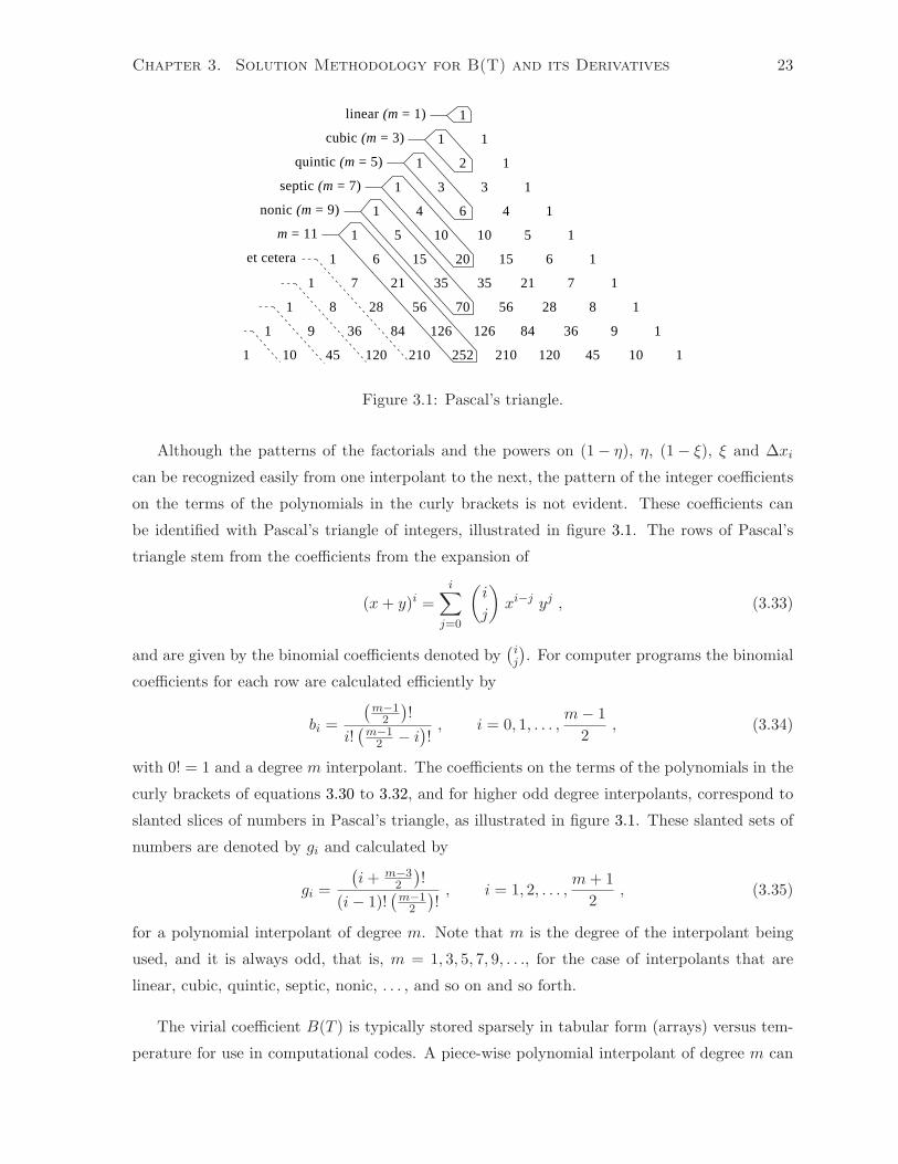
Although the patterns of the factorials and the powers on (1 − η), η, (1 − ξ), ξ and ∆xi
can be recognized easily from one interpolant to the next, the pattern of the integer coefficients
on the terms of the polynomials in the curly brackets is not evident. These coefficients can
be identified with Pascal’s triangle of integers, illustrated in figure 3.1. The rows of Pascal’s
triangle stem from the coefficients from the expansion of
(x + y)i =i
∑
j=0
(
i
j
)
xi−j yj , (3.33)
and are given by the binomial coefficients denoted by(
ij
)
. For computer programs the binomial
coefficients for each row are calculated efficiently by
bi =
(
m−12
)
!
i!(
m−12 − i
)
!, i = 0, 1, . . . ,
m − 1
2, (3.34)
with 0! = 1 and a degree m interpolant. The coefficients on the terms of the polynomials in the
curly brackets of equations 3.30 to 3.32, and for higher odd degree interpolants, correspond to
slanted slices of numbers in Pascal’s triangle, as illustrated in figure 3.1. These slanted sets of
numbers are denoted by gi and calculated by
gi =
(
i + m−32
)
!
(i − 1)!(
m−12
)
!, i = 1, 2, . . . ,
m + 1
2, (3.35)
for a polynomial interpolant of degree m. Note that m is the degree of the interpolant being
used, and it is always odd, that is, m = 1, 3, 5, 7, 9, . . ., for the case of interpolants that are
linear, cubic, quintic, septic, nonic, . . . , and so on and so forth.
The virial coefficient B(T ) is typically stored sparsely in tabular form (arrays) versus tem-
perature for use in computational codes. A piece-wise polynomial interpolant of degree m can
Chapter 3. Solution Methodology for B(T) and its Derivatives 24
be used to interpolate tabulated data for the second virial coefficient given by equation 3.1 only
when all derivatives up to and including the m−12 th derivative can be calculated.1 To control
the relative interpolation error between two adjacent nodes, an adaptive grid spacing is used.
This maximizes the size of each interval between two adjacent nodes such that the maximum
error in each interval equals a specified error tolerance.
A case study with a test function has been done in appendix A and the results show that
the size and storage space of the tabulated data is minimized when an adaptive grid spacing is
used. From the results presented in appendix A it was possible to derive that for a polynomial
interpolant of degree m that requires n nodes to capture a test function, the total storage space
for this special method of interpolation is given by
s =m + 3
2n . (3.36)
Here, 2n storage spaces are required to store data pairs of (xi, fi) for n nodes, and m−12 n storage
spaces are required to store m−12 derivatives of fi for n nodes, that is, df
dx
∣
∣
i, d2f
dx2
∣
∣
i, . . . , d
m−12 f
dxm−1
2
∣
∣
i,
as can easily be verified by inspection of equations 3.30, 3.31 and 3.32. In comparison to other
interpolation methods (such as those using Lagrange’s polynomials, Newton’s polynomials,
or splines)2 the piece-wise interpolation method typically requires fewer nodes to accurately
capture a given function based on a specified error tolerance, meaning that the storage space
of the tabulated data can be most effectively minimized when this method is used. In addition
to requiring fewer nodes, the piece-wise interpolation method is more accurate in general since
the values of the derivatives at adjacent nodes are known exactly, which is not the case in
comparison to other interpolation methods. For example, a cubic spline interpolation method
approximates the derivative values at the endpoints using either natural or clamped boundary
conditions which, although may ensure that the curvature along the spline in minimized, may
not ensure that the derivative values at each node are necessarily accurate.
3.6 Plots of the Integrands of B∗(T∗) and its Derivatives
Graphical illustrations of the integrands of B∗(T∗) and some of its lower derivatives are presented
in this section. This is done for the most important cases of intermolecular potentials of
Lennard-Jones in 1924, Buckingham and Corner in 1947 and Rice and Hirschfelder in 1954.
1See section 3.2.2The storage space for an interpolation method using Lagrange’s polynomials, Newton’s polynomials, or
splines is s = 2n + m(n − 1) for an interpolant of degree m using n nodes. Here, 2n storage spaces are requiredto store data pairs of (xi, fi) for n nodes, and m(n − 1) storage spaces are required to store m coefficients in(n − 1) node intervals.

Chapter 3. Solution Methodology for B(T) and its Derivatives 25
The primary reasons for showing these results is to illustrate the behaviour of these integrands,
show that they are relatively smooth (in regions between discontinuities, where applicable), and
further indicate the use of Gaussian quadrature integrations, as explained earlier in section 3.4.
For the classical second virial coefficient, the integrands for Bc(T∗) and its first, second and
third derivatives with respect to temperature are given by
cI0(x, T∗) = −f(x, T∗)[
1 + tan2(x)]
, (3.37)
cI1(x, T∗) =
{−1
T 2∗
}
[
f(x, T∗) + 1]
φ∗(x)[
1 + tan2(x)]
, (3.38)
cI2(x, T∗) =
{−φ∗(x)
T 4∗
+2
T 3∗
}
[
f(x, T∗) + 1]
φ∗(x)[
1 + tan2(x)]
, (3.39)
and
cI3(x, T∗) =
{−φ2∗(x)
T 6∗
+6φ∗(x)
T 5∗
− 6
T 4∗
}
[
f(x, T∗) + 1]
φ∗(x)[
1 + tan2(x)]
, (3.40)
respectively, and have been derived using the methodology presented earlier in section 3.2.1.
For the quantum correction to the second virial coefficient, the integrands for Bq(T∗) and its
first, second and third derivatives with respect to temperature are given by
qI0(x, T∗) =
{
1
T 3∗
}
F 2∗ (x)
[
f(x, T∗) + 1] [
1 + tan2(x)]
, (3.41)
qI1(x, T∗) =
{
φ∗(x)
T 5∗
− 3
T 4∗
}
F 2∗ (x)
[
f(x, T∗) + 1] [
1 + tan2(x)]
, (3.42)
qI2(x, T∗) =
{
φ2∗(x)
T 7∗
− 8φ∗(x)
T 6∗
+12
T 5∗
}
F 2∗ (x)
[
f(x, T∗) + 1] [
1 + tan2(x)]
, (3.43)
and
qI3(x, T∗) =
{
φ3∗(x)
T 9∗
− 15φ2∗(x)
T 8∗
+60φ∗(x)
T 7∗
− 60
T 6∗
}
F 2∗ (x)
[
f(x, T∗)+1] [
1 + tan2(x)]
, (3.44)
respectively, and have been derived using the methodology presented earlier in section 3.2.2.
The graphs for the integrands of Bc(T∗) and its first three derivatives are presented in figures
3.2, 3.3 and 3.4, for non-dimensional temperatures of 1.0, 10.0 and 100.0, respectively. The
graphs for the integrand of Bq(T∗) and its first three derivatives are presented in figures 3.5,
3.6 and 3.7, for non-dimensional temperatures of 1.0, 10.0 and 100.0, respectively.
For the Lennard-Jones 6-12 model, the integration is performed over the entire domain
[0, π2 ] since there are no discontinuities. For the modified Buckingham models of Buckingham
and Corner as well as Rice and Hirschfelder, the use of a composite integration method is
further justified through inspection of these graphs. When the modified Buckingham model
Chapter 3. Solution Methodology for B(T) and its Derivatives 26
of Buckingham and Corner is used, the discontinuity is present at x = π2 in the integrands of
the second virial coefficient. Although this is not evident graphically in the integrands which
have been presented, the discontinuity nonetheless exists and becomes more apparent in the
integrands of higher derivatives of the second virial coefficient. However, most evident is the
discontinuity present at x = tan−1(r3max/r3
min) in the integrands of the second virial coefficient
when the modified Buckingham model of Rice and Hirschfelder is used. In this specific case, the
integrand for the classical second virial coefficient within the domain [0, tan−1(r3max/r3
min)] is
given by[
1 + tan2(x)]
for Bc(T∗) and equal to zero for its derivatives, since φ(x) = ∞ and thus
f(x, T∗) = −1 when x < tan−1(r3max/r3
min) for this model. For similar reasons, the integrand
for the quantum correction is equal to zero within the domain [0, tan−1(r3max/r3
min)] for Bq(T∗)
and its derivatives because [ f(x, T∗) + 1] = 0.

Chapter 3. Solution Methodology for B(T) and its Derivatives 27
0 π/8 π/4 3π/8 π/2−4
0
2
x
cI0(x,T
*)
Buckingham and Corner modelRice and Hirschfelder modelLennard−Jones 6−12 model
0 π/8 π/4 3π/8 π/2−2
0
6
x
cI1(x,T
*)
0 π/8 π/4 3π/8 π/2−20
0
x
cI2(x,T
*)
0 π/8 π/4 3π/8 π/2
0
80
x
cI3(x,T
*)
Figure 3.2: Integrands of Bc(T∗) and its first three derivatives with T∗ = 1.0.

Chapter 3. Solution Methodology for B(T) and its Derivatives 28
0 π/8 π/4 3π/8 π/2
0
1
x
cI0(x,T
*)
Buckingham and Corner modelRice and Hirschfelder modelLennard−Jones 6−12 model
0 π/8 π/4 3π/8 π/2
−0.04
0
0.02
x
cI1(x,T
*)
0 π/8 π/4 3π/8 π/2
−0.005
0
0.005
x
cI2(x,T
*)
0 π/8 π/4 3π/8 π/2−0.002
0
0.002
x
cI3(x,T
*)
Figure 3.3: Integrands of Bc(T∗) and its first three derivatives with T∗ = 10.0.

Chapter 3. Solution Methodology for B(T) and its Derivatives 29
0 π/8 π/4 3π/8 π/2
0
1
x
cI0(x,T
*)
Buckingham and Corner modelRice and Hirschfelder modelLennard−Jones 6−12 model
0 π/8 π/4 3π/8 π/2
−0.004
0
x
cI1(x,T
*)
0 π/8 π/4 3π/8 π/2−0.00002
0
0.00006
x
cI2(x,T
*)
0 π/8 π/4 3π/8 π/2
−0.000001
0
0.000001
x
cI3(x,T
*)
Figure 3.4: Integrands of Bc(T∗) and its first three derivatives with T∗ = 100.0.

Chapter 3. Solution Methodology for B(T) and its Derivatives 30
0 π/8 π/4 3π/8 π/20
1500
x
qI0(x,T
*)
Buckingham and Corner modelRice and Hirschfelder modelLennard−Jones 6−12 model
0 π/8 π/4 3π/8 π/2
−3000
0
x
qI1(x,T
*)
0 π/8 π/4 3π/8 π/2
0
15000
x
qI2(x,T
*)
0 π/8 π/4 3π/8 π/2
−60000
0
20000
x
qI3(x,T
*)
Figure 3.5: Integrands of Bq(T∗) and its first three derivatives with T∗ = 1.0.

Chapter 3. Solution Methodology for B(T) and its Derivatives 31
0 π/8 π/4 3π/8 π/20
30
x
qI0(x,T
*)
Buckingham and Corner modelRice and Hirschfelder modelLennard−Jones 6−12 model
0 π/8 π/4 3π/8 π/2
−4
0
2
x
qI1(x,T
*)
0 π/8 π/4 3π/8 π/2
−0.5
0
1.5
x
qI2(x,T
*)
0 π/8 π/4 3π/8 π/2−0.5
0
0.5
x
qI3(x,T
*)
Figure 3.6: Integrands of Bq(T∗) and its first three derivatives with T∗ = 10.0.

Chapter 3. Solution Methodology for B(T) and its Derivatives 32
0 π/8 π/4 3π/8 π/20
2
x
qI0(x,T
*)
Buckingham and Corner modelRice and Hirschfelder modelLennard−Jones 6−12 model
0 π/8 π/4 3π/8 π/2
−0.02
0
0.02
x
qI1(x,T
*)
0 π/8 π/4 3π/8 π/2
−0.0005
0
0.0005
x
qI2(x,T
*)
0 π/8 π/4 3π/8 π/2
−0.00002
0
0.00002
x
qI3(x,T
*)
Figure 3.7: Integrands of Bq(T∗) and its first three derivatives with T∗ = 100.0.
Chapter 4
Results for B∗(T∗) and its
Derivatives
The numerical evaluation and interpolation methodology for the second virial coefficient and its
derivatives were presented in the previous chapter. Numerical results for B∗(T∗) and its deriva-
tives are given herein using this methodology for gaseous species and practical intermolecular
potential energy models. Second virial coefficient results for both Bc(T∗) and Bq(T∗) are in-
cluded to show their temperature-dependent behaviour and to illustrate the importance of the
quantum correction.
4.1 Numerical Solutions for B∗(T∗)
The application of the sophisticated method of interpolation using polynomial interpolants of
different degree m is presented for both the classical second virial coefficient Bc(T∗) as well as
the quantum correction Bq(T∗) to the second virial coefficient. Included are interpolants that
are cubic (m = 3), quintic (m = 5), septic (m = 7), nonic (m = 9), and so on and so forth,
up to m = 17. The relative error of the interpolated values is controlled to a specified value of
10−6 % using an adaptive grid spacing, meaning that the reconstructed solutions to the second
virial coefficient represented by interpolation are accurate to at least eight significant digits in
every interval between any two adjacent nodes throughout the entire domain.
The results are illustrated graphically for the specific cases of the Lennard-Jones 6-12
model and the modified Buckingham models of Buckingham and Corner as well as Rice and
33

Chapter 4. Results for B∗(T∗) and its Derivatives 34
Hirschfelder. A wide non-dimensional temperature (T∗) domain of [10−1, 104] was selected to
capture both light gases at elevated temperatures (T ≈ 100, 000 K) as well as heavy gases at low
temperatures (T ≈ 100 K). In general, lighter gases have lower values for ǫ/k whereas heavier
gases have larger ones [13], which, through the use of equation 3.6 for the expression represent-
ing the non-dimensional temperature, result in these bounding non-dimensional temperature
values.
4.1.1 Classical Second Virial Coefficient Bc(T∗)
The variation of the classical second virial coefficient Bc(T∗) is given as a function of the non-
dimensional temperature T∗ in figure 4.1, for the Lennard-Jones 6-12 model and the modified
Buckingham models of Buckingham and Corner as well as Rice and Hirschfelder. As illustrated
in this graph, the second virial coefficient is negative at low temperatures (the second virial
coefficient approaches negative infinity as the temperature tends towards zero) and positive at
high ones, passing through the Boyle temperature when the second virial coefficient is equal
to zero. The differences in the Bc(T∗) plots for the three different intermolecular potential
energy models at higher T∗ values are non-trivial. The classical second virial coefficient exhibits
the highest values for the Lennard-Jones 6-12 model, and the lowest values for the Rice and
Hirschfelder modified Buckingham (exponential-six) model. These results are in agreement
100
101
102
103
104
−1
0
0.6
T*
Bc(T
*)
8−
Buckingham and Corner modelRice and Hirschfelder modelLennard−Jones 6−12 model
Figure 4.1: The classical second virial coefficient.

Chapter 4. Results for B∗(T∗) and its Derivatives 35
with data in the literature [13, 6]. These differences are due to the high molecular speeds at
elevated temperatures, caused by the differences in the regions of the exponential repulsion in
the intermolecular potential energy models. The modified Buckingham model of Buckingham
and Corner is considered to be the most realistic of these three models for the calculation of
Bc(T∗), since it includes the most detailed account of molecular interactions while maintaining
a very high level of sophistication in the construction of the model itself.
The classical second virial coefficient Bc(T∗) is included using adaptive grid spacing for the
generation of tables. Graphs are used to illustrate the node locations, using an adaptive grid
spacing, for the minimum number of n nodes required to interpolate Bc(T∗) using a polynomial
interpolant of degree m. Once the number of n nodes are known for a polynomial interpolant of
degree m, the storage space of the tabulated data is calculated using s = m+32 n. The adaptive
grids for the classical second virial coefficient are illustrated graphically in figures 4.2 to 4.4, for
Lennard-Jones 6-12 model and the modified Buckingham models of Buckingham and Corner
as well as Rice and Hirschfelder, respectively. The adaptive grids and interpolations for Bc(T∗)
are done separately for each intermolecular potential energy model of interest, as a result of the
slight variations in the Bc(T∗) plots when different models are used.
Results for the Lennard-Jones 6-12 model are illustrated in figure 4.2. The number of nodes
10−1
100
101
102
103
104
−1
0
0.6
T*
Bc(T
*)
8−
m = 3 n = 646
m = 5 n = 138
m = 7 n = 65
m = 9 n = 42
m = 11 n = 31
m = 13 n = 25
m = 15 n = 22
m = 17 n = 19
Figure 4.2: Adaptive grid variation for new interpolation method for m = 3 , 5 , . . . , 17, using
the Lennard-Jones 6-12 model for the classical second virial coefficient.

Chapter 4. Results for B∗(T∗) and its Derivatives 36
required to generate an adaptive grid when polynomial interpolants of degree m = 3, 5, 7, 9,
11, 13, 15 and 17 are used are 646, 138, 65, 42, 31, 25, 22 and 19, respectively. In terms of
the storage space required in computer programs, the data storage is 1,938, 552, 325, 252, 217,
200, 198 and 190, respectively.
Results for the Buckingham and Corner modified Buckingham model are illustrated in figure
4.3. The number of nodes required to generate an adaptive grid when polynomial interpolants
of degree m = 3, 5, 7, 9, 11, 13, 15 and 17 are used are 667, 142, 66, 42, 31, 26, 22 and 20,
respectively. In terms of the storage space required in computer programs, the data storage
is 2,001, 568, 330, 252, 217, 208, 198 and 200, respectively. In this case, it becomes quite
apparent that it is not advantageous to use a polynomial interpolant of degree m = 17 because
the savings in data storage bottoms out when m = 15. Instead, it appears that the largest
savings in storage space occur when a quintic (m = 5) or septic (m = 7) interpolant is used.
10−1
100
101
102
103
104
−1
0
0.6
T*
Bc(T
*)
8−
m = 3 n = 667
m = 5 n = 142
m = 7 n = 66
m = 9 n = 42
m = 11 n = 31
m = 13 n = 26
m = 15 n = 22
m = 17 n = 20
Figure 4.3: Adaptive grid variation for new interpolation method for m = 3 , 5 , . . . , 17, using
the Buckingham and Corner modified Buckingham model (α = 13.5 and β = 0.0) for the
classical second virial coefficient.
Results for the Rice and Hirschfelder modified Buckingham (exponential-six) model are
illustrated in figure 4.4. The number of nodes required to generate an adaptive grid when
polynomial interpolants of degree m = 3, 5, 7, 9, 11, 13, 15 and 17 are used are 669, 142,
66, 42, 31, 26, 22 and 20, respectively. In terms of the storage space required in computer

Chapter 4. Results for B∗(T∗) and its Derivatives 37
programs, the data storage is 2,007, 568, 330, 252, 217, 208, 198 and 200, respectively. Once
again, it is not advantageous to use an interpolant of degree m = 17 because the savings in data
storage bottoms out when m = 15. Note that although the number of nodes required are equal
to the previous case, specifically for polynomial interpolants of degree m = 5 , 7 , . . . , 17, the
interpolations do not generate the exact same adaptive grids (e.g. non-dimensional temperature
values).
10−1
100
101
102
103
104
−1
0
0.6
T*
Bc(T
*)
8−
m = 3 n = 669
m = 5 n = 142
m = 7 n = 66
m = 9 n = 42
m = 11 n = 31
m = 13 n = 26
m = 15 n = 22
m = 17 n = 20
Figure 4.4: Adaptive grid variation for new interpolation method for m = 3 , 5 , . . . , 17, using
the Rice and Hirschfelder modified Buckingham (exponential-six) model (α = 13.5 and
β = 0.0) for the classical second virial coefficient.
The results of the adaptive grids for the classical second virial coefficient using polynomial
interpolants of different degree m = 3 , 5 , . . . , 17 show that the number of nodes required
to interpolate the tabulated data decreases as higher-degree interpolants are used. As for the
storage space of the tabulated data, the largest savings are seen when a quintic (m = 5) or septic
(m = 7) interpolant is used, and little to no savings are seen as polynomial interpolants upwards
of degree m = 17 are used. In other words, the savings in storage space eventually bottom out.
In smooth regions of the graph with relatively small curvature, such as when 101 ≤ T∗ ≤ 104
in figures 4.2, 4.3 and 4.4, the grid spacing between two adjacent nodes is large since the new
interpolant can efficiently capture the data over such a wide range of temperatures. As well,
in the specific case of cubic interpolation (m = 3), the large grid spacing near T∗ ≈ 102 can

Chapter 4. Results for B∗(T∗) and its Derivatives 38
easily be seen as a result of the function having an inflection point in the center of that region.
Lastly, it should be noted that these results validate that the derivatives of the classical second
virial coefficient have been derived and calculated accurately (as per section 3.2.1). Otherwise,
the results would not have shown a decrease in the number of nodes needed as the degree of
the polynomial interpolant was increasing.
The behaviour of the second virial coefficient can be better understood by taking a closer
look at the potential energy models which govern the behaviour of the interacting molecules.
At low temperatures the average energies of the molecules are on the order of the characteristic
energy, and colliding molecules exhibit behaviour similar to the molecular interactions within
the attractive region of the potential energy model. As a result, the second virial coefficient is
thus negative and there is a decrease in pressure in the gas. At high temperatures the average
energies of the molecules are relatively large in comparison to the characteristic energy, and
colliding molecules exhibit behaviour similar to the molecular interactions within the repulsive
region of the potential energy model. In this case, the second virial coefficient becomes positive
and the pressure of the gas increases. For very high temperatures, the intermolecular collisions
are so forceful that the molecules penetrate each other and behave as if they had a smaller
volume. This explains why the second virial coefficient has a maximum positive value, after
which it tends towards zero [13]. It also highlights the importance of accurately modeling
the repulsive interactions between molecules, and hints that small intricacies amongst different
intermolecular potential energy models do contribute noticeably to variations in Bc(T∗).
4.1.2 Quantum Correction Bq(T∗)
The variation of the quantum correction Bq(T∗) to the second virial coefficient is given as
a function of the non-dimensional temperature T∗ in figure 4.5, for the Lennard-Jones 6-12
model and the modified Buckingham models of Buckingham and Corner as well as Rice and
Hirschfelder. As mentioned earlier, the quantum correction to the second virial coefficient
accounts for the probability of the intermolecular potential energy configurations not being
proportional to the exponential term in equation 2.7. Hence, the quantum correction is positive
at all temperatures and approaches positive infinity as the temperature tends towards zero.
Similar to Bc(T∗), graphs of the quantum correction Bq(T∗) to the second virial coefficient
are included using adaptive grid spacing. The adaptive grids for the quantum correction to the
second virial coefficient are illustrated graphically in figures 4.6 to 4.8, for Lennard-Jones 6-12
model and the modified Buckingham models of Buckingham and Corner as well as Rice and
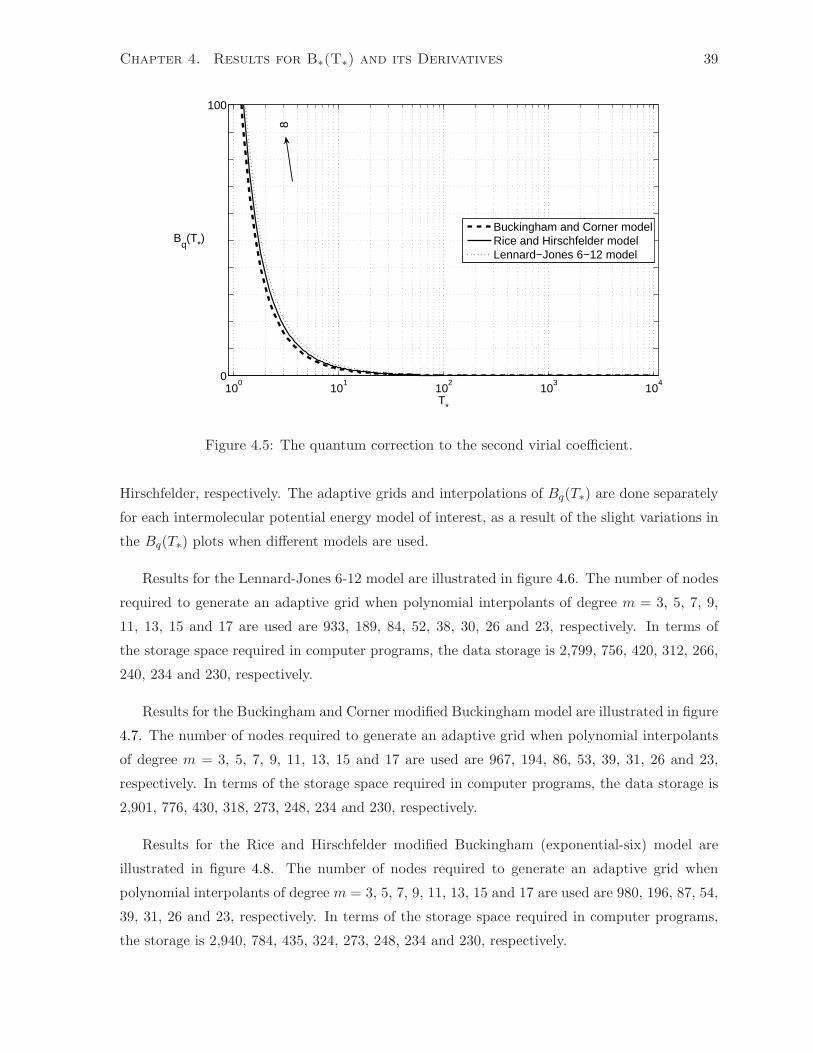
Chapter 4. Results for B∗(T∗) and its Derivatives 39
100
101
102
103
104
0
100
T*
Bq(T
*)
8
Buckingham and Corner modelRice and Hirschfelder modelLennard−Jones 6−12 model
Figure 4.5: The quantum correction to the second virial coefficient.
Hirschfelder, respectively. The adaptive grids and interpolations of Bq(T∗) are done separately
for each intermolecular potential energy model of interest, as a result of the slight variations in
the Bq(T∗) plots when different models are used.
Results for the Lennard-Jones 6-12 model are illustrated in figure 4.6. The number of nodes
required to generate an adaptive grid when polynomial interpolants of degree m = 3, 5, 7, 9,
11, 13, 15 and 17 are used are 933, 189, 84, 52, 38, 30, 26 and 23, respectively. In terms of
the storage space required in computer programs, the data storage is 2,799, 756, 420, 312, 266,
240, 234 and 230, respectively.
Results for the Buckingham and Corner modified Buckingham model are illustrated in figure
4.7. The number of nodes required to generate an adaptive grid when polynomial interpolants
of degree m = 3, 5, 7, 9, 11, 13, 15 and 17 are used are 967, 194, 86, 53, 39, 31, 26 and 23,
respectively. In terms of the storage space required in computer programs, the data storage is
2,901, 776, 430, 318, 273, 248, 234 and 230, respectively.
Results for the Rice and Hirschfelder modified Buckingham (exponential-six) model are
illustrated in figure 4.8. The number of nodes required to generate an adaptive grid when
polynomial interpolants of degree m = 3, 5, 7, 9, 11, 13, 15 and 17 are used are 980, 196, 87, 54,
39, 31, 26 and 23, respectively. In terms of the storage space required in computer programs,
the storage is 2,940, 784, 435, 324, 273, 248, 234 and 230, respectively.

Chapter 4. Results for B∗(T∗) and its Derivatives 40
10−1
100
101
102
103
104
0
100
T*
Bq(T
*)
8m = 3 n = 933
m = 5 n = 189
m = 7 n = 84
m = 9 n = 52
m = 11 n = 38
m = 13 n = 30
m = 15 n = 26
m = 17 n = 23
Figure 4.6: Adaptive grid variation for new interpolation method for m = 3 , 5 , . . . , 17, using
the Lennard-Jones 6-12 model for the quantum correction to the second virial coefficient.
10−1
100
101
102
103
104
0
100
T*
Bq(T
*)
8
m = 3 n = 967
m = 5 n = 194
m = 7 n = 86
m = 9 n = 53
m = 11 n = 39
m = 13 n = 31
m = 15 n = 26
m = 17 n = 23
Figure 4.7: Adaptive grid variation for new interpolation method for m = 3 , 5 , . . . , 17, using
the Buckingham and Corner modified Buckingham model (α = 13.5 and β = 0.0) for the
quantum correction to the second virial coefficient.
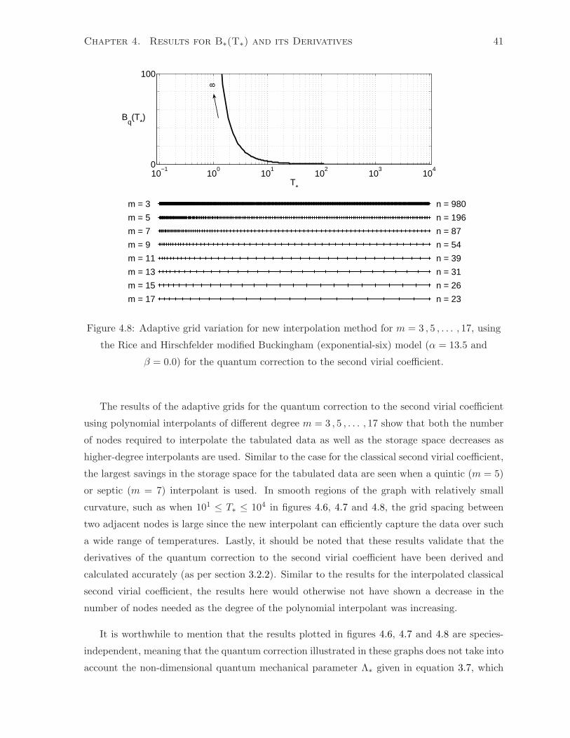
Chapter 4. Results for B∗(T∗) and its Derivatives 41
10−1
100
101
102
103
104
0
100
T*
Bq(T
*)
8m = 3 n = 980
m = 5 n = 196
m = 7 n = 87
m = 9 n = 54
m = 11 n = 39
m = 13 n = 31
m = 15 n = 26
m = 17 n = 23
Figure 4.8: Adaptive grid variation for new interpolation method for m = 3 , 5 , . . . , 17, using
the Rice and Hirschfelder modified Buckingham (exponential-six) model (α = 13.5 and
β = 0.0) for the quantum correction to the second virial coefficient.
The results of the adaptive grids for the quantum correction to the second virial coefficient
using polynomial interpolants of different degree m = 3 , 5 , . . . , 17 show that both the number
of nodes required to interpolate the tabulated data as well as the storage space decreases as
higher-degree interpolants are used. Similar to the case for the classical second virial coefficient,
the largest savings in the storage space for the tabulated data are seen when a quintic (m = 5)
or septic (m = 7) interpolant is used. In smooth regions of the graph with relatively small
curvature, such as when 101 ≤ T∗ ≤ 104 in figures 4.6, 4.7 and 4.8, the grid spacing between
two adjacent nodes is large since the new interpolant can efficiently capture the data over such
a wide range of temperatures. Lastly, it should be noted that these results validate that the
derivatives of the quantum correction to the second virial coefficient have been derived and
calculated accurately (as per section 3.2.2). Similar to the results for the interpolated classical
second virial coefficient, the results here would otherwise not have shown a decrease in the
number of nodes needed as the degree of the polynomial interpolant was increasing.
It is worthwhile to mention that the results plotted in figures 4.6, 4.7 and 4.8 are species-
independent, meaning that the quantum correction illustrated in these graphs does not take into
account the non-dimensional quantum mechanical parameter Λ∗ given in equation 3.7, which

Chapter 4. Results for B∗(T∗) and its Derivatives 42
is specific for a given molecular species. Although the values for the quantum correction to the
second virial coefficient are seemingly several orders of magnitude higher than the values for the
second virial coefficient itself are, the magnitude of the non-dimensional quantum mechanical
parameter Λ∗ is typically on the order of 10−3 for light gases (and smaller for heavier gases) and
balance out the corrective term quite nicely. These results are investigated further in section
4.2.
4.1.3 Selected Tabulated Solutions for B∗(T∗)
A selected set of tabulated second virial coefficient values are presented on the following six
pages for the specific case of nonic (m = 9) interpolation using an adaptive grid. Tables 4.1,
4.2 and 4.3 present the tabulated data for the classical second virial coefficient for the Lennard-
Jones 6-12 model, and the modified Buckingham models of Buckingham and Corner as well as
Rice and Hirschfelder, respectively, whereas tables 4.4, 4.5 and 4.6 present the tabulated data for
the quantum correction, for the respective intermolecular potential energy models mentioned.
This tabulated data for the second virial coefficient and its derivatives has been generated
using Wolfram Research’s Mathematica using a working precision of fifty significant digits, so
that it can be presented in tabular form accurate with a precision of at least fourteen significant
digits. The second virial coefficients have been calculated using non-dimensional temperature
values that are specified exactly to five significant digits. The truncations were done solely for
the purpose of being able to fit all of the numerical values for the second virial coefficient and its
first four derivatives, all of which are required for nonic (m = 9) interpolation, on one page. For
the same reason, the values for B∗(T∗) and its first four derivatives are presented only for the
last twenty-four temperature nodes for the interpolation, for both the second virial coefficient
Bc(T∗) and its quantum correction Bq(T∗).
The tabulated data given in tables 4.1 to 4.6 might be useful as a reference for researchers
when they generate their own tables for their computer programs using the methodology pre-
sented in this thesis. These tables can be constructed by the user and are expected to vary in
both size and storage space, based on the degree m polynomial interpolant which they choose,
as well as the specified error tolerance for the interpolations and the desired precision for the
final solutions.

Chapter
4.
Resu
lts
for
B∗ (T
∗ )and
its
Deriv
ativ
es
43
Table 4.1: Tabulated data for the classical second virial coefficient and its first four derivatives, using the Lennard-Jones 6-12 model,
interpolated using a nonic interpolant (m = 9).
T∗ Bc(T∗) B′
c(T∗) B′′
c (T∗) B(3)c (T∗) B
(4)c (T∗)
1.5859×100−7.5770649671212×10⁻¹ 9.9575958982251×10⁻¹
−1.5002119968127×100 3.3295809452847×100−9.8090160634466×100
2.0482×100−4.1678501662758×10⁻¹ 5.4510205648732×10⁻¹
−6.1933024679700×10⁻¹ 1.0293439768625×100−2.2686866615976×100
2.6377×100−1.7653500340634×10⁻¹ 3.0394768944427×10⁻¹
−2.6458346322809×10⁻¹ 3.3359327687058×10⁻¹−5.5660197427118×10⁻¹
3.3404×100−1.3358280895660×10⁻² 1.7689059174696×10⁻¹
−1.2135902914153×10⁻¹ 1.1909421153210×10⁻¹−1.5421226693208×10⁻¹
4.2279×100 1.0661394750451×10⁻¹ 1.0289766776797×10⁻¹−5.6255690999810×10⁻² 4.3264229231723×10⁻²
−4.3730262044929×10⁻²
5.5643×100 2.0675174859272×10⁻¹ 5.4152442586005×10⁻²−2.3065393923806×10⁻² 1.3450630338694×10⁻²
−1.0244099261307×10⁻²
7.5042×100 2.8034564489710×10⁻¹ 2.6211285321585×10⁻²−8.7163646739440×10⁻³ 3.7959124507214×10⁻³
−2.1379125736045×10⁻³
1.0320×101 3.2970006655030×10⁻¹ 1.1407475103606×10⁻²−3.0482915329031×10⁻³ 9.8517103116864×10⁻⁴
−4.0535077438327×10⁻⁴
1.4439×101 3.5887380266421×10⁻¹ 4.1244584334658×10⁻³−9.7343654212116×10⁻⁴ 2.3450559145372×10⁻⁴
−6.9996724844940×10⁻⁵
2.0525×101 3.7198751818992×10⁻¹ 8.6277197376693×10⁻⁴−2.7319177666771×10⁻⁴ 5.0407394720257×10⁻⁵
−1.0924016023828×10⁻⁵
2.9656×101 3.7273099121269×10⁻¹−3.9231485397914×10⁻⁴
−5.9705859406272×10⁻⁵ 9.3452688348393×10⁻⁶−1.4969161177679×10⁻⁶
4.3575×101 3.6414969167503×10⁻¹−7.2149032540526×10⁻⁴
−4.6646354759569×10⁻⁶ 1.3167080903696×10⁻⁶−1.6928507673382×10⁻⁷
6.5211×101 3.4870590360012×10⁻¹−6.7536654479036×10⁻⁴ 4.8682222725935×10⁻⁶ 5.8513741188906×10⁻⁸
−1.2822813540950×10⁻⁸
9.9709×101 3.2829606973800×10⁻¹−5.1398846312545×10⁻⁴ 4.0043469630654×10⁻⁶
−4.6031927041401×10⁻⁸ 2.4190194595730×10⁻¹⁰
1.5736×10² 3.0404106448254×10⁻¹−3.4596768057874×10⁻⁴ 2.0698973027715×10⁻⁶
−2.1843935758693×10⁻⁸ 3.1257149689546×10⁻¹⁰
2.6862×10² 2.7478883552673×10⁻¹−2.0269060729994×10⁻⁴ 7.9080390143547×10⁻⁷
−5.6103821108755×10⁻⁹ 5.7325488087083×10⁻¹¹
4.4364×10² 2.4794767170699×10⁻¹−1.1788480086835×10⁻⁴ 2.9441175094071×10⁻⁷
−1.3419100413380×10⁻⁹ 8.8806021384069×10⁻¹²
7.0826×10² 2.2416448805908×10⁻¹−6.9560094126444×10⁻⁵ 1.1246034419503×10⁻⁷
−3.3148162616145×10⁻¹⁰ 1.4199350073872×10⁻¹²
1.1146×10³ 2.0258805660272×10⁻¹−4.1136713096169×10⁻⁵ 4.3198523067264×10⁻⁸
−8.2548665910518×10⁻¹¹ 2.2912159102531×10⁻¹³
1.7404×10³ 1.8294085263883×10⁻¹−2.4313889483576×10⁻⁵ 1.6606887951042×10⁻⁸
−2.0602001609157×10⁻¹¹ 3.7092312460095×10⁻¹⁴
2.7080×10³ 1.6501118667219×10⁻¹−1.4330295101255×10⁻⁵ 6.3623979320724×10⁻⁹
−5.1221992657638×10⁻¹² 5.9798529573124×10⁻¹⁵
4.1940×10³ 1.4877763202060×10⁻¹−8.4494143289073×10⁻⁶ 2.4428358744867×10⁻⁹
−1.2788853147636×10⁻¹² 9.7019140294831×10⁻¹⁶
6.4794×10³ 1.3406332835360×10⁻¹−4.9773310255547×10⁻⁶ 9.3748296606395×10⁻¹⁰
−3.1937864411275×10⁻¹³ 1.5757118110284×10⁻¹⁶
1.0000×10⁴ 1.2072270784154×10⁻¹−2.9268101771440×10⁻⁶ 3.5897586497377×10⁻¹⁰
−7.9562463582650×10⁻¹⁴ 2.5524962732946×10⁻¹⁷

Chapter
4.
Resu
lts
for
B∗ (T
∗ )and
its
Deriv
ativ
es
44
Table 4.2: Tabulated data for the classical second virial coefficient and its first four derivatives, using the Buckingham and Corner
modified Buckingham model (α = 13.5 and β = 0.0), interpolated using a nonic interpolant (m = 9).
T∗ Bc(T∗) B′
c(T∗) B′′
c (T∗) B(3)c (T∗) B
(4)c (T∗)
1.8950×100−4.8335762118751×10⁻¹ 6.3051470700076×10⁻¹
−7.8360829168924×10⁻¹ 1.4240190080524×100−3.4312157982458×100
2.4431×100−2.2610154222205×10⁻¹ 3.4848128063953×10⁻¹
−3.3065406335271×10⁻¹ 4.5404280948364×10⁻¹−8.2505706935959×10⁻¹
3.1144×100−4.9129833722863×10⁻² 1.9878438305246×10⁻¹
−1.4751174964869×10⁻¹ 1.5626519612627×10⁻¹−2.1840162490945×10⁻¹
3.8221×100 6.2009935413131×10⁻² 1.2368326357057×10⁻¹−7.5300463168082×10⁻² 6.4448937820987×10⁻²
−7.2523082954831×10⁻²
4.9724×100 1.6681228970185×10⁻¹ 6.6638296553456×10⁻²−3.1913321888298×10⁻² 2.0914456170348×10⁻²
−1.7911238846617×10⁻²
6.6473×100 2.4570979889300×10⁻¹ 3.2861245997411×10⁻²−1.2371459527387×10⁻² 6.0959195059965×10⁻³
−3.8879041098070×10⁻³
9.0764×100 2.9952029209265×10⁻¹ 1.4548655142562×10⁻²−4.4243695614676×10⁻³ 1.6260281793251×10⁻³
−7.6169921341445×10⁻⁴
1.2612×101 3.3176141881927×10⁻¹ 5.3745409970356×10⁻³−1.4481202027934×10⁻³ 3.9839252806074×10⁻⁴
−1.3605833884486×10⁻⁴
1.7804×101 3.4656797716372×10⁻¹ 1.1803462506703×10⁻³−4.1910822014638×10⁻⁴ 8.8511144558846×10⁻⁵
−2.2043721451721×10⁻⁵
2.5552×101 3.4773723315555×10⁻¹−4.8255300835031×10⁻⁴
−9.5998449629434×10⁻⁵ 1.7069647494800×10⁻⁵−3.1483910269394×10⁻⁶
3.7240×101 3.3845812014104×10⁻¹−9.4731392806614×10⁻⁴
−9.5193207717154×10⁻⁶ 2.5766043260861×10⁻⁶−3.7825842197230×10⁻⁷
5.5226×101 3.2133363519849×10⁻¹−9.1240954001362×10⁻⁴ 6.8748404369696×10⁻⁶ 1.6181609459799×10⁻⁷
−3.2032276301449×10⁻⁸
8.3532×101 2.9839089669295×10⁻¹−7.1307523821374×10⁻⁴ 6.2699742945010×10⁻⁶
−7.6873749012210×10⁻⁸−6.1626889234317×10⁻¹¹
1.2974×10² 2.7097764101188×10⁻¹−4.9517795412694×10⁻⁴ 3.4545050350387×10⁻⁶
−4.2251784130216×10⁻⁸ 6.8716133844333×10⁻¹⁰
2.1304×10² 2.3869358536373×10⁻¹−3.0676920285409×10⁻⁴ 1.4642480158436×10⁻⁶
−1.2658500164588×10⁻⁸ 1.5761046654429×10⁻¹⁰
3.5236×10² 2.0617128841876×10⁻¹−1.8025900820851×10⁻⁴ 5.5884849668461×10⁻⁷
−3.1321591557528×10⁻⁹ 2.5529083860038×10⁻¹¹
5.5635×10² 1.7788282140707×10⁻¹−1.0809022044366×10⁻⁴ 2.2251640202102×10⁻⁷
−8.2121561976008×10⁻¹⁰ 4.4012336251292×10⁻¹²
8.6199×10² 1.5245396266212×10⁻¹−6.4836125540948×10⁻⁵ 8.9383532964664×10⁻⁸
−2.1888223014705×10⁻¹⁰ 7.7565076566939×10⁻¹³
1.3205×10³ 1.2960970516626×10⁻¹−3.8741678099271×10⁻⁵ 3.5959795312441×10⁻⁸
−5.8753217624011×10⁻¹¹ 1.3839881203416×10⁻¹³
2.0061×10³ 1.0924223740127×10⁻¹−2.3039868034426×10⁻⁵ 1.4464412703806×10⁻⁸
−1.5842470602313×10⁻¹¹ 2.4927879090325×10⁻¹⁴
3.0236×10³ 9.1292352877398×10⁻²−1.3653964316743×10⁻⁵ 5.8298970185600×10⁻⁹
−4.3037898634021×10⁻¹² 4.5487526872695×10⁻¹⁵
4.5334×10³ 7.5550810014222×10⁻²−8.0439003868310×10⁻⁶ 2.3453348613188×10⁻⁹
−1.1712494067930×10⁻¹² 8.3453934816546×10⁻¹⁶
6.7553×10³ 6.1927700073224×10⁻²−4.7188706878696×10⁻⁶ 9.4497938917086×10⁻¹⁰
−3.2091282509493×10⁻¹³ 1.5493361880671×10⁻¹⁶
1.0000×10⁴ 5.0273416779209×10⁻²−2.7585275023367×10⁻⁶ 3.8203221019663×10⁻¹⁰
−8.8771797421975×10⁻¹⁴ 2.9213187823347×10⁻¹⁷
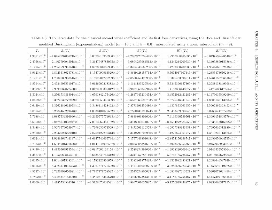
Chapter
4.
Resu
lts
for
B∗ (T
∗ )and
its
Deriv
ativ
es
45
Table 4.3: Tabulated data for the classical second virial coefficient and its first four derivatives, using the Rice and Hirschfelder
modified Buckingham (exponential-six) model (α = 13.5 and β = 0.0), interpolated using a nonic interpolant (m = 9).
T∗ Bc(T∗) B′
c(T∗) B′′
c (T∗) B(3)c (T∗) B
(4)c (T∗)
1.9351×100−4.6452597068215×10⁻¹ 6.0023216955906×10⁻¹
−7.2982423739445×10⁻¹ 1.2957868465635×100−3.0497539428540×100
2.4958×100−2.1407795945018×10⁻¹ 3.3147648783065×10⁻¹
−3.0804285984513×10⁻¹ 4.1345214209639×10⁻¹−7.3405889015386×10⁻¹
3.1795×100−4.2551596961540×10⁻² 1.8923081865990×10⁻¹
−1.3784045566258×10⁻¹ 1.4293860702030×10⁻¹−1.9544668152613×10⁻¹
3.9323×100 6.8925518675781×10⁻² 1.1547090963529×10⁻¹−6.8619428157714×10⁻² 5.7074917107145×10⁻²
−6.2355473676216×10⁻²
5.1261×100 1.7007808938515×10⁻¹ 6.1692904225289×10⁻²−2.8880952423966×10⁻² 1.8378433896811×10⁻²
−1.5261150766316×10⁻²
6.8594×100 2.4534903531017×10⁻¹ 3.0126600218383×10⁻²−1.1141183526540×10⁻² 5.3345366157360×10⁻³
−3.2988138849368×10⁻³
9.3699×100 2.9599632877420×10⁻¹ 1.3120080305012×10⁻²−3.9627050342915×10⁻³ 1.4183306448677×10⁻³
−6.4473608617355×10⁻⁴
1.3024×101 3.2561736315014×10⁻¹ 4.6591842175426×10⁻³−1.2847645230474×10⁻³ 3.4572912421287×10⁻⁴
−1.1476035509269×10⁻⁴
1.8409×101 3.3827839777959×10⁻¹ 8.3320850448389×10⁻⁴−3.6337660593763×10⁻⁴ 7.5775416941240×10⁻⁵
−1.8385135113095×10⁻⁵
2.6439×101 3.3762484662023×10⁻¹−6.3486114428492×10⁻⁴
−7.8771391256480×10⁻⁵ 1.4307873963955×10⁻⁵−2.5902365398452×10⁻⁶
3.8565×101 3.2684459269543×10⁻¹−1.0033404075562×10⁻³
−4.7850433199074×10⁻⁶ 2.0433489093945×10⁻⁶−3.0263674767762×10⁻⁷
5.7188×101 3.0857534316996×10⁻¹−9.2350575771643×10⁻⁴ 7.8838809804606×10⁻⁶ 7.9139390759561×10⁻⁸
−2.3699151805776×10⁻⁸
8.6560×101 2.8478741008247×10⁻¹−7.0513262461182×10⁻⁴ 6.3418080041021×10⁻⁶
−8.4554272885955×10⁻⁸ 5.7838113816398×10⁻¹⁰
1.3488×10² 2.5673579053997×10⁻¹−4.7996639973509×10⁻⁴ 3.3472509116355×10⁻⁶
−4.0907388343931×10⁻⁸ 6.7695616312880×10⁻¹⁰
2.2510×10² 2.2342525668210×10⁻¹−2.8759122295313×10⁻⁴ 1.3419793728960×10⁻⁶
−1.1272624961777×10⁻⁸ 1.3613249113675×10⁻¹⁰
3.6624×10² 1.9248364744137×10⁻¹−1.6947740665734×10⁻⁴ 5.1757649801648×10⁻⁷
−2.8454156258747×10⁻⁹ 2.2659656944735×10⁻¹¹
5.7373×10² 1.6544901301698×10⁻¹−1.0147544992587×10⁻⁴ 2.0603388381691×10⁻⁷
−7.4923536955368×10⁻¹⁰ 3.9452958953327×10⁻¹²
8.8426×10² 1.4120562975544×10⁻¹−6.0817609139154×10⁻⁵ 8.2588324292690×10⁻⁸
−1.9968230609940×10⁻¹⁰ 6.9742435555064×10⁻¹³
1.3477×10³ 1.1952080815301×10⁻¹−3.6435843762312×10⁻⁵ 3.3247952786119×10⁻⁸
−5.3766135726757×10⁻¹¹ 1.2516052672583×10⁻¹³
2.0395×10³ 1.0014667338261×10⁻¹−2.1782126806659×10⁻⁵ 1.3382961877429×10⁻⁸
−1.4503982383821×10⁻¹¹ 2.2688646587949×10⁻¹⁴
3.0616×10³ 8.3023171031393×10⁻²−1.3027371776502×10⁻⁵ 5.4477986926971×10⁻⁹
−3.9286636223036×10⁻¹² 4.1453649119278×10⁻¹⁵
4.5737×10³ 6.7926992650981×10⁻²−7.7157471758532×10⁻⁶ 2.2543524805633×10⁻⁹
−1.0809087613527×10⁻¹² 7.5307072631498×10⁻¹⁶
6.7802×10³ 5.4984346163530×10⁻²−4.4810516369670×10⁻⁶ 9.4496307384341×10⁻¹⁰
−3.1186755256187×10⁻¹³ 1.4447392166415×10⁻¹⁶
1.0000×10⁴ 4.4185736504316×10⁻²−2.5158673631521×10⁻⁶ 3.8807601035027×10⁻¹⁰
−9.1250649438875×10⁻¹⁴ 2.9232686377135×10⁻¹⁷
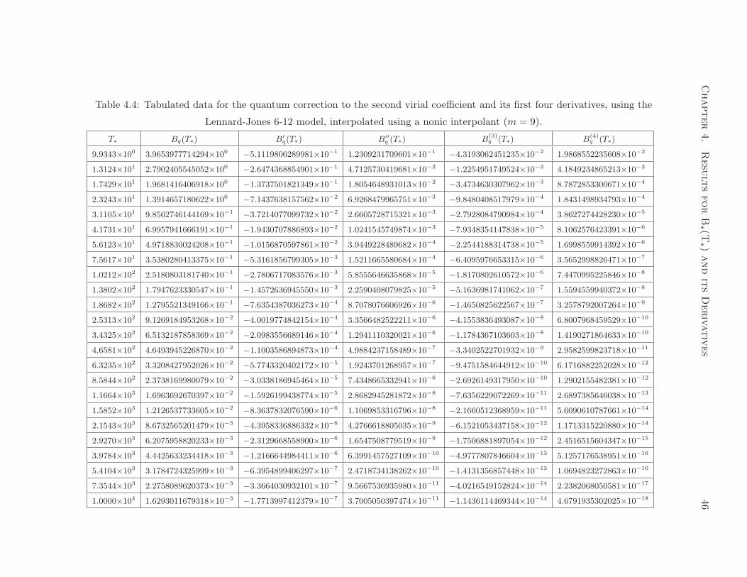
Chapter
4.
Resu
lts
for
B∗ (T
∗ )and
its
Deriv
ativ
es
46
Table 4.4: Tabulated data for the quantum correction to the second virial coefficient and its first four derivatives, using the
Lennard-Jones 6-12 model, interpolated using a nonic interpolant (m = 9).
T∗ Bq(T∗) B′
q(T∗) B′′
q (T∗) B(3)q (T∗) B
(4)q (T∗)
9.9343×100 3.9653977714294×100−5.1119806289981×10⁻¹ 1.2309231709601×10⁻¹
−4.3193062451235×10⁻² 1.9868552235608×10⁻²
1.3124×101 2.7902405545052×100−2.6474368854901×10⁻¹ 4.7125730419681×10⁻²
−1.2254951749524×10⁻² 4.1849234865213×10⁻³
1.7429×101 1.9681416406918×100−1.3737501821349×10⁻¹ 1.8054648931013×10⁻²
−3.4734630307962×10⁻³ 8.7872853300671×10⁻⁴
2.3243×101 1.3914657180622×100−7.1437638157562×10⁻² 6.9268479965751×10⁻³
−9.8480408517979×10⁻⁴ 1.8431498934793×10⁻⁴
3.1105×101 9.8562746144169×10⁻¹−3.7214077099732×10⁻² 2.6605728715321×10⁻³
−2.7928084790984×10⁻⁴ 3.8627274428230×10⁻⁵
4.1731×101 6.9957941666191×10⁻¹−1.9430707886893×10⁻² 1.0241545749874×10⁻³
−7.9348354147838×10⁻⁵ 8.1062576423391×10⁻⁶
5.6123×101 4.9718830024208×10⁻¹−1.0156870597861×10⁻² 3.9449228489682×10⁻⁴
−2.2544188314738×10⁻⁵ 1.6998559914392×10⁻⁶
7.5617×101 3.5380280413375×10⁻¹−5.3161856799305×10⁻³ 1.5211665580684×10⁻⁴
−6.4095976653315×10⁻⁶ 3.5652998826471×10⁻⁷
1.0212×10² 2.5180803181740×10⁻¹−2.7806717083576×10⁻³ 5.8555646635868×10⁻⁵
−1.8170802610572×10⁻⁶ 7.4470995225846×10⁻⁸
1.3802×10² 1.7947623330547×10⁻¹−1.4572636945550×10⁻³ 2.2590408079825×10⁻⁵
−5.1636981741062×10⁻⁷ 1.5594559940372×10⁻⁸
1.8682×10² 1.2795521349166×10⁻¹−7.6354387036273×10⁻⁴ 8.7078076606926×10⁻⁶
−1.4650825622567×10⁻⁷ 3.2578792007264×10⁻⁹
2.5313×10² 9.1269184953268×10⁻²−4.0019774842154×10⁻⁴ 3.3566482522211×10⁻⁶
−4.1553836493087×10⁻⁸ 6.8007968459529×10⁻¹⁰
3.4325×10² 6.5132187858369×10⁻²−2.0983556689146×10⁻⁴ 1.2941110320021×10⁻⁶
−1.1784367103603×10⁻⁸ 1.4190271864633×10⁻¹⁰
4.6581×10² 4.6493945226870×10⁻²−1.1003586894873×10⁻⁴ 4.9884237158489×10⁻⁷
−3.3402522701932×10⁻⁹ 2.9582599823718×10⁻¹¹
6.3235×10² 3.3208427952026×10⁻²−5.7743320402172×10⁻⁵ 1.9243701268957×10⁻⁷
−9.4751584644912×10⁻¹⁰ 6.1716882252028×10⁻¹²
8.5844×10² 2.3738169980079×10⁻²−3.0338186945464×10⁻⁵ 7.4348665332941×10⁻⁸
−2.6926149317950×10⁻¹⁰ 1.2902155482381×10⁻¹²
1.1664×10³ 1.6963692670397×10⁻²−1.5926199438774×10⁻⁵ 2.8682945281872×10⁻⁸
−7.6356229072269×10⁻¹¹ 2.6897385646038×10⁻¹³
1.5852×10³ 1.2126537733605×10⁻²−8.3637832076590×10⁻⁶ 1.1069853316796×10⁻⁸
−2.1660512368959×10⁻¹¹ 5.6090610787661×10⁻¹⁴
2.1543×10³ 8.6732565201479×10⁻³−4.3958336886332×10⁻⁶ 4.2766618805035×10⁻⁹
−6.1521053437158×10⁻¹² 1.1713315220880×10⁻¹⁴
2.9270×10³ 6.2075958820233×10⁻³−2.3129668558900×10⁻⁶ 1.6547508779519×10⁻⁹
−1.7506881897054×10⁻¹² 2.4516515604347×10⁻¹⁵
3.9784×10³ 4.4425633234418×10⁻³−1.2166644984411×10⁻⁶ 6.3991457527109×10⁻¹⁰
−4.9777807846604×10⁻¹³ 5.1257176538951×10⁻¹⁶
5.4104×10³ 3.1784724325999×10⁻³−6.3954899406297×10⁻⁷ 2.4718734138262×10⁻¹⁰
−1.4131356857448×10⁻¹³ 1.0694823272863×10⁻¹⁶
7.3544×10³ 2.2758089620373×10⁻³−3.3664030932101×10⁻⁷ 9.5667536935980×10⁻¹¹
−4.0216549152824×10⁻¹⁴ 2.2382068050581×10⁻¹⁷
1.0000×10⁴ 1.6293011679318×10⁻³−1.7713997412379×10⁻⁷ 3.7005050397474×10⁻¹¹
−1.1436114469344×10⁻¹⁴ 4.6791935302025×10⁻¹⁸

Chapter
4.
Resu
lts
for
B∗ (T
∗ )and
its
Deriv
ativ
es
47
Table 4.5: Tabulated data for the quantum correction to the second virial coefficient and its first four derivatives, using the
Buckingham and Corner modified Buckingham model (α = 13.5 and β = 0.0), interpolated using a nonic interpolant (m = 9).
T∗ Bq(T∗) B′
q(T∗) B′′
q (T∗) B(3)q (T∗) B
(4)q (T∗)
1.2456×101 1.9054228373148×100−2.0771844192762×10⁻¹ 4.0818146779135×10⁻²
−1.1529808815410×10⁻² 4.2417149532369×10⁻³
1.6417×101 1.3154274304246×100−1.0632308362371×10⁻¹ 1.5573937054008×10⁻²
−3.2850696357375×10⁻³ 9.0336619020696×10⁻⁴
2.1729×101 9.1032004678422×10⁻¹−5.4462999047734×10⁻² 5.9379429547452×10⁻³
−9.3406334753481×10⁻⁴ 1.9171524172441×10⁻⁴
2.8847×101 6.3199879307263×10⁻¹−2.7956775892642×10⁻² 2.2663598579360×10⁻³
−2.6567180564087×10⁻⁴ 4.0669726108081×10⁻⁵
3.8408×101 4.3998818321656×10⁻¹−1.4371107667628×10⁻² 8.6473362911744×10⁻⁴
−7.5445623436123×10⁻⁵ 8.6045767685531×10⁻⁶
5.1239×101 3.0734703552900×10⁻¹−7.4102419717979×10⁻³ 3.3046105277514×10⁻⁴
−2.1438396584174×10⁻⁵ 1.8204538523339×10⁻⁶
6.8500×101 2.1523308768306×10⁻¹−3.8312972292121×10⁻³ 1.2635839898958×10⁻⁴
−6.0845329996266×10⁻⁶ 3.8419093160629×10⁻⁷
9.1717×101 1.5105835397096×10⁻¹−1.9888809822431×10⁻³ 4.8433840075652×10⁻⁵
−1.7279142668423×10⁻⁶ 8.1021853575417×10⁻⁸
1.2304×10² 1.0605235191311×10⁻¹−1.0355796315680×10⁻³ 1.8596656495225×10⁻⁵
−4.9026454366382×10⁻⁷ 1.7031227084007×10⁻⁸
1.6531×10² 7.4381091619134×10⁻²−5.4089862941443×10⁻⁴ 7.1663777472641×10⁻⁶
−1.3935387644646×10⁻⁷ 3.5780025743142×10⁻⁹
2.2236×10² 5.2030058548816×10⁻²−2.8309653137424×10⁻⁴ 2.7742196614600×10⁻⁶
−3.9781179174263×10⁻⁸ 7.5361250250708×10⁻¹⁰
2.9940×10² 3.6232724011091×10⁻²−1.4810880319658×10⁻⁴ 1.0775510129177×10⁻⁶
−1.1413206378717×10⁻⁸ 1.5946963853890×10⁻¹⁰
4.0327×10² 2.5097934560486×10⁻²−7.7326012968505×10⁻⁵ 4.1948798570766×10⁻⁷
−3.2937093211536×10⁻⁹ 3.4012724389680×10⁻¹¹
5.4353×10² 1.7266948829840×10⁻²−4.0149540183939×10⁻⁵ 1.6288456971018×10⁻⁷
−9.5128611390545×10⁻¹⁰ 7.2809345491114×10⁻¹²
7.3207×10² 1.1811842127838×10⁻²−2.0754618068991×10⁻⁵ 6.3136937024669×10⁻⁸
−2.7529326528852×10⁻¹⁰ 1.5680610266201×10⁻¹²
9.8549×10² 8.0313317173796×10⁻³−1.0668166813996×10⁻⁵ 2.4363833856655×10⁻⁸
−7.9483924116614×10⁻¹¹ 3.3790157667731×10⁻¹³
1.3240×10³ 5.4384382911862×10⁻³−5.4697341813721×10⁻⁶ 9.3948205653084×10⁻⁹
−2.2987930816553×10⁻¹¹ 7.3163423735795×10⁻¹⁴
1.7763×10³ 3.6650467630643×10⁻³−2.7943087713010×10⁻⁶ 3.6129861975630×10⁻⁹
−6.6385186696840×10⁻¹² 1.5843047017741×10⁻¹⁴
2.3792×10³ 2.4588834567192×10⁻³−1.4236274487431×10⁻⁶ 1.3873405091239×10⁻⁹
−1.9164614696125×10⁻¹² 3.4342495697032×10⁻¹⁵
3.1815×10³ 1.6420227943114×10⁻³−7.2349371494211×10⁻⁷ 5.3215186930964×10⁻¹⁰
−5.5335226895338×10⁻¹³ 7.4547741847363×10⁻¹⁶
4.2461×10³ 1.0915514371216×10⁻³−3.6704871219699×10⁻⁷ 2.0417503635333×10⁻¹⁰
−1.6008671778584×10⁻¹³ 1.6239908072230×10⁻¹⁶
5.6597×10³ 7.2128594757926×10⁻⁴−1.8558074961043×10⁻⁷ 7.8198235533680×10⁻¹¹
−4.6289608810678×10⁻¹⁴ 3.5398520045708×10⁻¹⁷
7.5322×10³ 4.7363066212458×10⁻⁴−9.3541605090162×10⁻⁸ 2.9922135491335×10⁻¹¹
−1.3395761341842×10⁻¹⁴ 7.7341319991164×10⁻¹⁸
1.0000×10⁴ 3.0919730944999×10⁻⁴−4.7080023241006×10⁻⁸ 1.1469886132311×10⁻¹¹
−3.8942736150612×10⁻¹⁵ 1.7018506134245×10⁻¹⁸

Chapter
4.
Resu
lts
for
B∗ (T
∗ )and
its
Deriv
ativ
es
48
Table 4.6: Tabulated data for the quantum correction to the second virial coefficient and its first four derivatives, using the Rice and
Hirschfelder modified Buckingham (exponential-six) model (α = 13.5 and β = 0.0), interpolated using a nonic interpolant (m = 9).
T∗ Bq(T∗) B′
q(T∗) B′′
q (T∗) B(3)q (T∗) B
(4)q (T∗)
1.3920×101 1.9910885624200×100−1.9053680429934×10⁻¹ 3.2773082996347×10⁻²
−8.1375588659958×10⁻³ 2.6396511738030×10⁻³
1.8414×101 1.3756334462553×100−9.8031017273921×10⁻² 1.2552664102098×10⁻²
−2.3217615308186×10⁻³ 5.6138685717655×10⁻⁴
2.4432×101 9.5120652366190×10⁻¹−5.0534012446031×10⁻² 4.8192729324982×10⁻³
−6.6404866363118×10⁻⁴ 1.1966088259240×10⁻⁴
3.2509×101 6.5752394974659×10⁻¹−2.6057006119030×10⁻² 1.8507894957783×10⁻³
−1.8993085934149×10⁻⁴ 2.5494756650600×10⁻⁵
4.3348×101 4.5427965864971×10⁻¹−1.3439405913836×10⁻² 7.1115387320489×10⁻⁴
−5.4354370578760×10⁻⁵ 5.4342043684328×10⁻⁶
5.7895×101 3.1358947128009×10⁻¹−6.9315375599062×10⁻³ 2.7334968219470×10⁻⁴
−1.5562764759229×10⁻⁵ 1.1588914962892×10⁻⁶
7.7418×101 2.1621531516473×10⁻¹−3.5740942937824×10⁻³ 1.0508685687281×10⁻⁴
−4.4578072955009×10⁻⁶ 2.4728108782173×10⁻⁷
1.0364×10² 1.4880938730178×10⁻¹−1.8410254775755×10⁻³ 4.0369381724468×10⁻⁵
−1.2760591664766×10⁻⁶ 5.2729275013105×10⁻⁸
1.3880×10² 1.0225692079134×10⁻¹−9.4808106169589×10⁻⁴ 1.5516105933128×10⁻⁵
−3.6568774481911×10⁻⁷ 1.1262266621620×10⁻⁸
1.8593×10² 7.0129096313541×10⁻²−4.8796301257270×10⁻⁴ 5.9650258868406×10⁻⁶
−1.0488697983834×10⁻⁷ 2.4088258168420×10⁻⁹
2.4902×10² 4.7995461259877×10⁻²−2.5107489534260×10⁻⁴ 2.2949824542616×10⁻⁶
−3.0134456224790×10⁻⁸ 5.1650015255051×10⁻¹⁰
3.3364×10² 3.2734962371830×10⁻²−1.2891890219860×10⁻⁴ 8.8152137327905×10⁻⁷
−8.6459451733637×10⁻⁹ 1.1061736448930×10⁻¹⁰
4.4669×10² 2.2266207554801×10⁻²−6.6189428080784×10⁻⁵ 3.3905673243558×10⁻⁷
−2.4872349157914×10⁻⁹ 2.3782453138670×10⁻¹¹
5.9783×10² 1.5084650290064×10⁻²−3.3935980030727×10⁻⁵ 1.3035934203769×10⁻⁷
−7.1589933678832×10⁻¹⁰ 5.1199166887912×10⁻¹²
7.9928×10² 1.0176994313926×10⁻²−1.7395905003449×10⁻⁵ 5.0184147920426×10⁻⁸
−2.0666413903575×10⁻¹⁰ 1.1069850727090×10⁻¹²
1.0682×10³ 6.8215328778710×10⁻³−8.9011053531281×10⁻⁶ 1.9287893442276×10⁻⁸
−5.9649072001372×10⁻¹¹ 2.3946320066874×10⁻¹³
1.4263×10³ 4.5353092163320×10⁻³−4.5548574428197×10⁻⁶ 7.4051707765574×10⁻⁹
−1.7230560766051×10⁻¹¹ 5.2013107573856×10⁻¹⁴
1.9005×10³ 2.9827971640231×10⁻³−2.3416722971220×10⁻⁶ 2.8547721519632×10⁻⁹
−4.9824587226626×10⁻¹² 1.1379396511713×10⁻¹⁴
2.5282×10³ 1.9243614321582×10⁻³−1.2072870046075×10⁻⁶ 1.1137134216547×10⁻⁹
−1.4421420800972×10⁻¹² 2.4714828238152×10⁻¹⁵
3.3554×10³ 1.2063081086605×10⁻³−6.1842046001871×10⁻⁷ 4.4363466408784×10⁻¹⁰
−4.2834209047848×10⁻¹³ 5.4059710552161×10⁻¹⁶
4.4364×10³ 7.2972738094339×10⁻⁴−3.0976429909368×10⁻⁷ 1.7842302843782×10⁻¹⁰
−1.3286719339116×10⁻¹³ 1.2482689333132×10⁻¹⁶
5.8432×10³ 4.2420795149732×10⁻⁴−1.4926416599057×10⁻⁷ 7.0280362462850×10⁻¹¹
−4.1810063746098×10⁻¹⁴ 3.0445402327031×10⁻¹⁷
7.6689×10³ 2.3709084738858×10⁻⁴−6.8678829921274×10⁻⁸ 2.6496568767863×10⁻¹¹
−1.2797672570426×10⁻¹⁴ 7.4555448697369×10⁻¹⁸
1.0000×10⁴ 1.2890037517233×10⁻⁴−3.0518168739997×10⁻⁸ 9.6142047219172×10⁻¹²
−3.7817006152412×10⁻¹⁵ 1.7852285013427×10⁻¹⁸

Chapter 4. Results for B∗(T∗) and its Derivatives 49
4.2 Quantum Correction to B∗(T∗) for H2 and N2
A comparison of the classical second virial coefficient to the second virial coefficient with the
quantum correction taken into account is illustrated graphically in figure 4.9. This investigation
is performed using the non-dimensional temperature domain of [10−1, 104], using the same
reasoning as described in the previous section. The results illustrated in figure 4.9 are presented
for the gases hydrogen (H2) and nitrogen (N2), using the Lennard-Jones 6-12 model. Similar
results have be obtained when the modified Buckingham models of Buckingham and Corner as
well as Rice and Hirschfelder were used. The values for the force constants (σ and ǫ) are unique
to the Lennard-Jones 6-12 model and taken as defined in the technical report by Svehla [32].
The light gas hydrogen has been chosen to illustrate the significance of the quantum correction
on the second virial coefficient, since the quantum effects are significant for lighter gases at low
temperatures. Nitrogen has been chosen to illustrate the effects of the quantum correction on
a heavier gas, and also due to its abundance in the earth’s atmosphere. It should be noted
that currently none of the major computational codes account for quantum corrections in their
equations of state used to model gaseous species, and use only the classical term in the second
virial coefficient.
100
101
102
103
104
−1
0
0.6
T*
B*(T
*)
8−
B*(T
*) for H
2 B
*(T
*) for N
2 B
c(T
*)
Figure 4.9: The significance of the quantum correction to the second virial coefficient.
It is evident through inspection of figure 4.9 that the quantum correction is not only impor-
tant at low temperatures but that it in fact trails into the results at higher temperatures. The
Chapter 4. Results for B∗(T∗) and its Derivatives 50
quantum correction is most influential in the non-dimensional temperature domain of T∗ ≤ 25,
which corresponds roughly to a temperature domain of T ≤ 1, 500 K for the specific case of
hydrogen gas, and T ≤ 1, 750 K for the specific case of nitrogen gas. In comparison to the
quantum correction for hydrogen gas, the quantum correction for nitrogen gas is much smaller
in magnitude and is indistinguishable graphically from the classical curve. This shows that
the quantum correction is sufficiently significant for the second virial coefficient and should be
taken into account at all temperatures for light gases. For relatively heavier gases the quantum
correction is not as significant, and the solution for the second virial coefficient tends towards
the classical curve as the gas becomes heavier. It should be noted that the results presented in
figure 4.9 agree well with similar trends that are found in literature, both graphically [8, 13, 17]
and in tabular form [4], for the quantum correction to the second virial coefficient.

Chapter 5
Concluding Remarks
This study has presented an accurate and efficient method for the evaluation of the second
temperature-dependent virial coefficient B(T ) and its derivatives, for gaseous species and prac-
tical intermolecular potential energy models, used in the virial equation of state for imperfect
gases. This methodology consists of the following primary developments:
• A very accurate numerical integration method has been presented for the computation
of the integrals associated with B(T ) and its derivatives. Gaussian quadrature has been
used in conjunction with the software package developed by Wolfram Research called
Mathematica, using as large of an n-point rule as necessary to obtain final solutions
accurate to as many significant digits as required.
• A new method of polynomial interpolation of arbitrary degree m has been presented for
the evaluation of B(T ) and its derivatives stored in tables as discrete data Ti, Bi(Ti),
B′i(Ti), . . . , B
(m−12 )
i (Ti), for i = 1, 2, 3, . . . , n for n nodes.
• The minimization of stored data for B(T ) and its derivatives in computer programs using
an adaptive grid to control the relative error of interpolated values and make it the same
for each selected segment of the adaptive grid.
It has been shown in this thesis that B(T ) and its derivatives can be computed easily not only
for the conventional classical Lennard-Jones 6-12 model but also for the modified Buckingham
models of Buckingham and Corner as well as Rice and Hirschfelder. This work has also shown
that the quantum correction to the second virial coefficient can be incorporated easily in ad-
ditional calculations and tabulations of B(T ) and its derivatives, and that this correction is a
51
Chapter 5. Concluding Remarks 52
significant adjustment to the classical second virial coefficient for lighter gases such as hydrogen
(H2).
The same methodology can be used to evaluate the third temperature-dependent virial
coefficient C(T ) and its derivatives, along with its quantum corrections, and construct tables
for storage in computer programs, in virtually the same manner as for B(T ) and its derivatives.
One difficulty is that the numerical evaluation of C(T ) and its derivatives involves triple integrals
and therefore requires the use of multi-dimensional numerical integration techniques.

References
[1] Abramowitz, M., and Stegun, I. A. Handbook of Mathematical Functions: with For-
mulas, Graphs, and Mathematical Tables. Dover, 1972.
[2] Benedict, M., Webb, G. B., and Rubin, L. C. An Empirical Equation for Thermody-
namic Properties of Light Hydrocarbons and their Mixtures, I. Methane, Ethane, Propane
and n-Butane. Jour. Chem. Phys., 8(4), 334-345, 1940.
[3] Beth, E., and Uhlenbeck, G. E. The Quantum Theory of the Non-Ideal Gas. II.
Behaviour at Low Temperatures. Physica, 4(10), 915-924, 1937.
[4] Buckingham, R. A., and Corner, J. Tables of Second Virial and Low-Pressure Joule-
Thomson Coefficients for Intermolecular Potentials with Exponential Repulsion. Proc. R.
Soc. Lond. A, 189, 118-129, 1947.
[5] Corbin, N., Meath, W. J., and Allnatt, A. R. Second Virial Coefficients, Including
Quantum Corrections, for Nitrogen using Model Potentials. Mole. Phys., 53(1), 225-232,
1984.
[6] Dymond, J. H., and Smith, E. B. The Virial Coefficients of Gases; A Critical Compi-
lation. Oxford Clarendon Press, 1969.
[7] Forsythe, G. E., Malcolm, M. A., and Moler, C. B. Computer Methods for
Mathematical Computations. Prentice-Hall, 1977.
[8] Fowler, R. H. Statistical Mechanics: the Theory of the Properties of Matter in Equilib-
rium, 2e. Cambridge University Press, 1936.
[9] Freedman, E. Blake- A Thermodynamic Code Based on Tiger: User’s Guide and Manual.
Technical Report ARBRL–TR–02411, Ballistic Research Laboratory, US Army Armament
Research and Development Command, AD/A–121–259, 1982.
53
References 54
[10] Gordon, S., and McBride, B. J. Computer Program for Computation of Complex
Chemical Equilibrium Compositions, Rocket Performance, Incident and Reflected Shocks,
and Chapman-Jouguet Detonations. National Aeronautics and Space Administration
(NASA) NASA-SP-273, 1971.
[11] Gottlieb, J. J., and Hryniewicki, M. K. Polynomial Interpolation for a Function
and its Lower Derivatives Available from Tables. Preparation of a paper for publication,
Institute for Aerospace Studies, University of Toronto, 2010.
[12] Gropper, L. Quantum Theory of the Equation of State at Low Temperatures. Phys. Rev.,
50, 963-974, 1936.
[13] Hirschfelder, J. O., Curtiss, C. F., and Bird, R. B. Molecular Theory of Gases
and Liquids. New York Wiley, 1954.
[14] Jones, J. E. On the Determination of Molecular Fields. II. From the Equation of State
of a Gas. Proc. R. Soc. Lond. A, 106(738), 463-477, 1924.
[15] Kihara, T. Determination of Intermolecular Forces from the Equation of State of Gases.
Jour. Phys. Soc. Japan, 3, 265-268, 1947.
[16] Kihara, T. Virial Coefficients and Models of Molecules in Gases B. Rev. Mod. Phys.,
27(4), 412-423, 1955.
[17] Kim, S., and Henderson, D. Quantum Corrections to the Third and Fourth Virial
Coefficients using the 6:12 Potential. Proc. Natl. Acad. Sci. U.S.A., 55, 705-708, 1966.
[18] Kirkwood, J. G. Quantum Statistics of Almost Classical Assemblies. Phys. Rev., 44,
31-37, 1933.
[19] Lagrange, J.-L. Mecanique Analytique. 1811, Courcier. Reissued by Cambridge Univer-
sity Press, 2009.
[20] Mayer, J. E., and Mayer, M. G. Statistical Mechanics. John Wiley and Sons, Inc.,
1940.
[21] McFall, J. H., Wilson, D. S., and Lee, L. L. Accurate Correlation of the Second
Virial Coefficients of Some 40 Chemicals Based on an Anisotropic Square Well Potential.
Ind. and Eng. Chem. Research, 41, 1107-1112, 2002.
[22] Press, W. H., Teukolsky, S. A., Vetterling, W. T., and Flannery, B. P. Nu-
merical Recipes in FORTRAN: the Art of Scientific Computing, 2e. Cambridge University
Press, 1992.
References 55
[23] Redlich, O., and Kwong, J. N. S. On the Thermodynamics of Solutions. V. An
Equation of State. Fugacities of Gaseous Solutions. Chem. Rev., 44(1), 233-234, 1949.
[24] Ree, F. H. A Statistical Mechanical Theory of Chemically Reacting Multiphase Mixtures:
Application to the Detonation Properties of PETN. Jour. Chem. Phys., 81(3), 1251-1263,
1984.
[25] Ree, F. H. Supercritical Fluid Phase Separations: Implications for Detonation Properties
of Condensed Explosives. Jour. Chem. Phys., 84(10), 5845-5856, 1986.
[26] Reid, R. C., Prausnitz, J. M., and Poling, B. E. The Properties of Gases and
Liquids, 4e. McGraw-Hill, Inc., 1987.
[27] Rice, W. E., and Hirschfelder, J. O. Second Virial Coefficients of Gases Obeying a
Modified Buckingham (Exp-Six) Potential. Jour. Chem. Phys., 22(2), 187-192, 1954.
[28] Slater, J. C. The Quantum Theory of the Equation of State. Phys. Rev., 38, 237-242,
1931.
[29] Smith, W. R., and Missen, R. W. Chemical Reaction Equilibrium Analysis: Theory
and Algorithms. Krieger Publishing Company, 1991.
[30] Soave, G. Equilibrium Constants from a Modified Redlich-Kwong Equation of State.
Chem. Eng. Sci., 27, 1197-1203, 1972.
[31] Starling, K. E. Thermo Data Refined for LPG, Part 1: Equation of State and Computer
Prediction. Hydroc. Process., 50(3), 101-104, 1971.
[32] Svehla, R. A. Estimated Viscosities and Thermal Conductivities of Gases at High Tem-
peratures. National Aeronautics and Space Administration (NASA) NASA-TR-R-132,
1962.
[33] Uhlenbeck, G. E., and Beth, E. The Quantum Theory of the Non-Ideal Gas. I.
Deviations from the Classical Theory. Physica, 3(1), 729-745, 1936.
[34] Uhlenbeck, G. E., and Gropper, L. The Equation of State of a Non-ideal Einstein-
Bose or Fermi-Dirac Gas. Phys. Rev., 41, 79-90, 1932.
[35] van der Waals, J. D. Over de Continuiteit van den Gas - en Vloeistoftoestand (On the
Continuity of the Gas and Liquid State). Ph.D. Thesis, Leiden, The Netherlands, 1873.
[36] Vincenti, W. G., and Kruger, C. H. Introduction to Physical Gas Dynamics. New
York Wiley, 1965.

References 56
[37] Wigner, E. On the Quantum Correction for Thermodynamic Equilibrium. Phys. Rev.,
40, 749-759, 1932.
[38] Wong, F. C. H., Gottlieb, J. J., and Lussier, L.-S. Chemical Equilibrium Analysis
of Combustion Products at Constant Volume. Defence R & D Canada – Valcartier Technical
Report DRDC Valcartier TR-2003-375, 2003.

Appendix A
Assessment of New Interpolation
Method
The high-degree polynomial interpolation method for tabulated data that was presented in
section 3.5 is illustrated and assessed in this appendix. The theory presented in section 3.5
is not repeated here. Instead, the new method of polynomial interpolation is compared to
conventional interpolation methods using Lagrange’s polynomials [19] and polynomial splines
[7] of the same degree, in order to illustrate and assess the advantages of numerical efficiency.
This includes the ease of using the new interpolant and the resulting reduction in the size of
the tabulated data that needs to be stored in computational codes.
A set of tabulated data is required for the comparisons and assessments of different inter-
polation methods. This tabulated data is generated by the analytical function
y(x) =1 + 8x
1 + (4x)4(A.1)
on the domain [0, 1], so that the function and its derivatives are readily and accurately available
for the assessments. The behaviour of this test function and its first four derivatives is illustrated
in figure A.1. The test function is smooth and has no discontinuities in the function itself or its
higher derivatives. However, the test function has a maximum, a point of inflection and strong
curvature in some places to make accurate interpolation challenging. The higher derivatives are
highly fluctuating, include several local maxima and minima, include several inflection points,
and their amplitudes are not constant or negligibly small. Most importantly, the test function
is continuously differentiable, providing the opportunity to assess the interpolation methods for
an unrestricted range of high-degree interpolants.
57

Appendix A. Assessment of New Interpolation Method 58
Figure A.1: Plots of the test function and its first four derivatives.
The interpolation of tabulated data is studied for both uniformly and non-uniformly dis-
tributed data. For the data yi = y(xi) distributed uniformly with xi (e.g., uniform grid), where
i = 1, 2, . . . , n for n discrete data pairs, the objective is to reduce the constant interval width
∆x = xi+1 − xi such that the maximum relative interpolation error given by
E =
∣
∣
∣
∣
yexact(x) − yinterpolant(x)
yexact(x)
∣
∣
∣
∣
× 100% (A.2)
at any location x in any interval over the entire domain does not exceed 10−9 %. Symbolically,
Emax[0,1] = 10−9 %. For the data yi = y(xi) distributed non-uniformly with xi (e.g., adaptive grid),
the objective is to determine the minimum number n of discrete data pairs, where i = 1, 2, . . . , n,
such that the maximum error at any location x in every interval between two adjacent nodes
equals 10−9 %, that is Emaxi=1 ,2 ,... ,n−1 = 10−9 %. This maximum allowable error ensures that the

Appendix A. Assessment of New Interpolation Method 59
reconstructed solutions represented by interpolation are accurate to at least eleven significant
digits. For the case of the adaptive grid, this maximizes each interval and significantly reduces
the storage of the data xi, y(xi), y′(xi), y′′(xi), . . . , for i = 1, 2, . . . , n.
The results of this investigation are summarized in table A.1, and they provide a comparison
and assessment of various polynomial interpolation methods of different degree m. Included
are interpolants that are linear (m = 1), cubic (m = 3), quintic (m = 5), septic (m = 7), and
so on and so forth, up to m = 17. The advantages of using the new method of interpolation
over conventional interpolation methods using Lagrange’s polynomials and polynomial splines
are clearly evident from a study of the data. Consider the specific case of linear interpolation
Table A.1: Numbers of nodes and tabulated data required for interpolation of tabulated data
by various polynomial interpolation methods of different degrees (m).
degree of interpolant interpolation methoduniform grid adaptive grid
nodes (n) data (s) nodes (n) data (s)
m = 1
Lagrange 91,564 274,691 59,577 178,730
spline 91,564 274,691 59,577 178,730
new interpolant 91,564 183,128 59,577 119,154
m = 3
Lagrange 873 4,362 528 2,637
spline 700 3,497 308 1,537
new interpolant 505 1,515 305 915
m = 5Lagrange 222 1,549 128 891
new interpolant 91 364 52 208
m = 7Lagrange 136 1,217 70 623
new interpolant 39 195 23 115
m = 9Lagrange 107 1,168 52 563
new interpolant 23 138 13 78
m = 11Lagrange 93 1,198 45 574
new interpolant 17 119 10 70
m = 13Lagrange 88 1,307 42 617
new interpolant 13 104 8 64
m = 15Lagrange 87 1,464 38 631
new interpolant 11 99 7 63
m = 17Lagrange 87 1,636 37 686
new interpolant 9 90 6 60
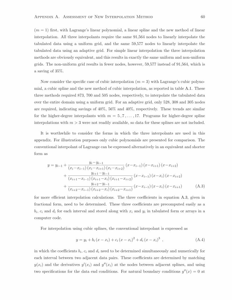
Appendix A. Assessment of New Interpolation Method 60
(m = 1) first, with Lagrange’s linear polynomial, a linear spline and the new method of linear
interpolation. All three interpolants require the same 91,564 nodes to linearly interpolate the
tabulated data using a uniform grid, and the same 59,577 nodes to linearly interpolate the
tabulated data using an adaptive grid. For simple linear interpolation the three interpolation
methods are obviously equivalent, and this results in exactly the same uniform and non-uniform
grids. The non-uniform grid results in fewer nodes, however, 59,577 instead of 91,564, which is
a saving of 35%.
Now consider the specific case of cubic interpolation (m = 3) with Lagrange’s cubic polyno-
mial, a cubic spline and the new method of cubic interpolation, as reported in table A.1. These
three methods required 873, 700 and 505 nodes, respectively, to interpolate the tabulated data
over the entire domain using a uniform grid. For an adaptive grid, only 528, 308 and 305 nodes
are required, indicating savings of 40%, 56% and 40%, respectively. These trends are similar
for the higher-degree interpolants with m = 5 , 7 , . . . , 17. Programs for higher-degree spline
interpolations with m > 3 were not readily available, so data for these splines are not included.
It is worthwhile to consider the forms in which the three interpolants are used in this
appendix. For illustration purposes only cubic polynomials are presented for comparison. The
conventional interpolant of Lagrange can be expressed alternatively in an equivalent and shorter
form as
y = yi−1 +yi−yi−1
(xi−xi−1) (xi−xi+1) (xi−xi+2)(x−xi−1) (x−xi+1) (x−xi+2)
+yi+1−yi−1
(xi+1−xi−1) (xi+1−xi) (xi+1−xi+2)(x−xi−1) (x−xi) (x−xi+2)
+yi+2−yi−1
(xi+2−xi−1) (xi+2−xi) (xi+2−xi+1)(x−xi−1) (x−xi) (x−xi+1) (A.3)
for more efficient interpolation calculations. The three coefficients in equation A.3, given in
fractional form, need to be determined. These three coefficients are precomputed easily as a
bi, ci and di for each interval and stored along with xi and yi in tabulated form or arrays in a
computer code.
For interpolation using cubic splines, the conventional interpolant is expressed as
y = yi + bi (x − xi) + ci (x − xi)2 + di (x − xi)
3 , (A.4)
in which the coefficients bi, ci and di need to be determined simultaneously and numerically for
each interval between two adjacent data pairs. These coefficients are determined by matching
y(xi) and the derivatives y′(xi) and y′′(xi) at the nodes between adjacent splines, and using
two specifications for the data end conditions. For natural boundary conditions y′′(x) = 0 at

Appendix A. Assessment of New Interpolation Method 61
each end node; for clamped boundary conditions y′(x) is specified at each end node; for this
work y′′(x1) and y′′(xn) are determined at each data end from the cubic polynomial fitted to
the limit and last four data pairs, respectively. This latter approach is superior for engineering
and science applications. These three coefficients bi, ci and di are then stored in tabular form
or arrays along with xi and yi in a computer code.
For the new method of interpolation, the cubic interpolant can be expressed as
y =1
0!y∣
∣
i(1 − η)2 η0 {1 + 2η}∆x0
i +(−1)0
0!y∣
∣
i+1(1 − ξ)2 ξ0 {1 + 2ξ}∆x0
i
+1
1!
dy
dx
∣
∣
∣
∣
i
(1 − η)2 η1 {1}∆x1i +
(−1)1
1!
dy
dx
∣
∣
∣
∣
i+1
(1 − ξ)2 ξ1 {1}∆x1i , (A.5)
as derived in section 3.5. Only the data xi, yi and y′(xi) are stored in tabular form or arrays
in a computer code.
When a function is stored in tabular form (arrays) for interpolation in computational codes,
the focus of attention should shift from the total number of nodes used to the number of data
stored in the program. The storage space is usually minimized to reduce the program size. For
interpolation using Lagrange’s polynomials and polynomial splines, the number of stored data
is s = 2n + m(n− 1) for an interpolant of degree m using n nodes. Here, 2n storage spaces are
required to store the data pairs (xi, yi) for n nodes, and m(n − 1) storage spaces are required
to store m coefficients for (n − 1) node intervals. For interpolation using the new method, the
storage is considerably less, given by s = m+32 n. Here, 2n storage spaces are required to store
data pairs (xi, yi) for n nodes, and m−12 n storage spaces are required to store m−1
2 derivatives of
yi for n nodes, that is, dydx
∣
∣
i, d2y
dx2
∣
∣
i, . . . , d
m−12 y
dxm−1
2
∣
∣
i. Revisiting the specific case of cubic interpolation
(m = 3) in table A.1, interpolants based on Lagrange’s polynomials, cubic splines and the new
method of interpolation require 4,362, 3,497 and 1,515 computer storage spaces, respectively,
for a uniform grid. For an adaptive grid, the corresponding computer storage is 2,637, 1,537
and 915, respectively, yielding savings of 40%, 56% and 40%, respectively. The reduction in
storage for interpolations with higher-degree polynomials is obvious from the results in table
A.1.
Fewer nodes are required to interpolate the tabulated data when an adaptive grid is used in
place of a uniform grid. A uniform grid ensures that the maximum error amongst all intervals
in the entire domain is less than or equal to a specified error(
10−9 %)
, which normally occurs at
one location in the entire domain, whereas an adaptive grid maximizes the size of each interval
such that the maximum error in each interval equals the specified error(
10−9 %)
. The trend of
fewer nodes for a non-uniform grid is obvious in the results in table A.1. Furthermore, a direct
comparison of the number of nodes required to interpolate the tabulated data using various
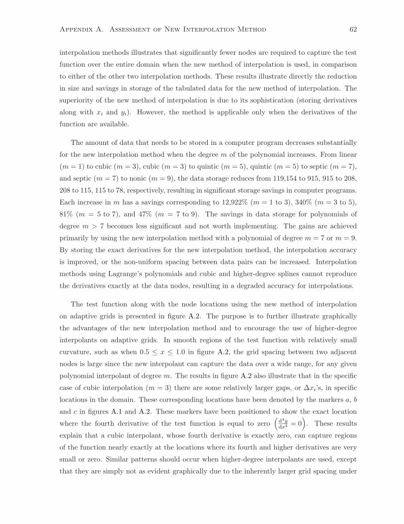
Appendix A. Assessment of New Interpolation Method 62
interpolation methods illustrates that significantly fewer nodes are required to capture the test
function over the entire domain when the new method of interpolation is used, in comparison
to either of the other two interpolation methods. These results illustrate directly the reduction
in size and savings in storage of the tabulated data for the new method of interpolation. The
superiority of the new method of interpolation is due to its sophistication (storing derivatives
along with xi and yi). However, the method is applicable only when the derivatives of the
function are available.
The amount of data that needs to be stored in a computer program decreases substantially
for the new interpolation method when the degree m of the polynomial increases. From linear
(m = 1) to cubic (m = 3), cubic (m = 3) to quintic (m = 5), quintic (m = 5) to septic (m = 7),
and septic (m = 7) to nonic (m = 9), the data storage reduces from 119,154 to 915, 915 to 208,
208 to 115, 115 to 78, respectively, resulting in significant storage savings in computer programs.
Each increase in m has a savings corresponding to 12,922% (m = 1 to 3), 340% (m = 3 to 5),
81% (m = 5 to 7), and 47% (m = 7 to 9). The savings in data storage for polynomials of
degree m > 7 becomes less significant and not worth implementing. The gains are achieved
primarily by using the new interpolation method with a polynomial of degree m = 7 or m = 9.
By storing the exact derivatives for the new interpolation method, the interpolation accuracy
is improved, or the non-uniform spacing between data pairs can be increased. Interpolation
methods using Lagrange’s polynomials and cubic and higher-degree splines cannot reproduce
the derivatives exactly at the data nodes, resulting in a degraded accuracy for interpolations.
The test function along with the node locations using the new method of interpolation
on adaptive grids is presented in figure A.2. The purpose is to further illustrate graphically
the advantages of the new interpolation method and to encourage the use of higher-degree
interpolants on adaptive grids. In smooth regions of the test function with relatively small
curvature, such as when 0.5 ≤ x ≤ 1.0 in figure A.2, the grid spacing between two adjacent
nodes is large since the new interpolant can capture the data over a wide range, for any given
polynomial interpolant of degree m. The results in figure A.2 also illustrate that in the specific
case of cubic interpolation (m = 3) there are some relatively larger gaps, or ∆xi’s, in specific
locations in the domain. These corresponding locations have been denoted by the markers a, b
and c in figures A.1 and A.2. These markers have been positioned to show the exact location
where the fourth derivative of the test function is equal to zero(
d4ydx4 = 0
)
. These results
explain that a cubic interpolant, whose fourth derivative is exactly zero, can capture regions
of the function nearly exactly at the locations where its fourth and higher derivatives are very
small or zero. Similar patterns should occur when higher-degree interpolants are used, except
that they are simply not as evident graphically due to the inherently larger grid spacing under

Appendix A. Assessment of New Interpolation Method 63
Figure A.2: Test function and illustration of adaptive grid variation for new interpolation
method for m = 3 , 5 , . . . , 17.
such conditions.
Although the use of the new method of interpolation results in significantly lower storage
requirements in computational codes when higher-degree interpolants are used, the equation
for the interpolant can increase in length and complexity. For example, for septic (m = 7)
interpolation between two adjacent data pairs, the interpolant is given by
y =1
0!y∣
∣
i(1−η)
4η0
{
1+4η+10η2+20η3}
∆x0i
+(−1)0
0!y∣
∣
i+1(1−ξ)
4ξ0
{
1+4ξ+10ξ2+20ξ3}
∆x0i
+1
1!
dy
dx
∣
∣
∣
∣
i
(1−η)4η1
{
1+4η+10η2}
∆x1i
+(−1)1
1!
dy
dx
∣
∣
∣
∣
i+1
(1−ξ)4ξ1
{
1+4ξ+10ξ2}
∆x1i
+1
2!
d2y
dx2
∣
∣
∣
∣
i
(1−η)4η2 {1+4η}∆x2
i+
(−1)2
2!
d2y
dx2
∣
∣
∣
∣
i+1
(1−ξ)4ξ2 {1+4ξ}∆x2
i
+1
3!
d3y
dx3
∣
∣
∣
∣
i
(1−η)4η3 {1}∆x3
i+
(−1)3
3!
d3y
dx3
∣
∣
∣
∣
i+1
(1−ξ)4ξ3 {1}∆x3
i, (A.6)
in full symbolic notation from the derivation given in section 3.5. The calculations of this
interpolant, however, can be simplified and minimized in computer codes. The procedure can
be automated for an interpolant of arbitrary degree m by simply using a cleverly-written set of
nested loops.