ABSTRACT

Title of dissertation: ESSAYS IN EXPERIMENTALECONOMICS WITH IMPLICATIONSFOR ECONOMIC DEVELOPMENT

Kahwa C. Douoguih, Doctor of Philosophy, 2011

Dissertation directed by: Professor Maureen Cropper andProfessor Erkut OzbayDepartment of Economics

In an exploration of the joint concerns of economic development, namely e�ciency

and equality, I employ experimental methods to consider several issues regarding

entrepreneurship and regulation with particular applications in developing countries.

Entrepreneurship programs in developing countries may not take hold in rural

populations if people there tend to shy away from competitive and uncertain economic

opportunities, thus contributing to the systematic underdevelopment of rural areas.

In a �eld experiment conducted among potential entrepreneurs in rural and urban

Ghana, we found that rural subjects were 20 percent less likely than their urban

counterparts to select an all-or-nothing tournament compensation scheme over a piece

rate wage to per- form a simple matching task. The di�erence between the rural and

urban tournament choice was driven by subjects who believed their own performance

was the best within their group; urban subjects were twice as likely as their rural

counterparts to believe that they had scored in �rst place and were thus more likely

to select the tournament compensation.

To examine behavior in a tax setting, we develop a simple tax evasion model as

a signaling game between a taxpayer and an auditor that includes a non-strategic,

always compliant taxpayer. In addition to the taxpayer's income report to the auditor,

he has the option to send a costly message, a donation to charity that may serve as

an indirect signal to the auditor of the taxpayer's ethical type. In the case where

the taxpayer has misreported his income and is audited, he must pay unpaid taxes

and a penalty. We establish a Perfect Bayesian equilibrium where taxpayers will use

the charitable donation to signal honesty, thereby reducing the probability of audit.

Auditors will optimally audit reports without charity donations more frequently than

those with donations. To test our theoretical predictions, we use a two-sided signaling

experiment where the taxpayer voluntarily reports his income to determine his tax

liability and can make an observable and veri�able charity donation. Our aggregate

experimental results indicate players employ mixed strategies in line with theoretical

predictions.

ESSAYS IN EXPERIMENTAL ECONOMICS WITH IMPLICATIONSFOR ECONOMIC DEVELOPMENT

by

Kahwa Catharine Douoguih

Dissertation submitted to the Faculty of the Graduate School of theUniversity of Maryland, College Park in partial ful�llment

of the requirements for the degree ofDoctor of Philosophy

2011

Advisory Committee:Professor Maureen Cropper, Co-Chair/AdvisorProfessor Erkut Ozbay, Co-Chair/AdvisorProfessor Emel Filiz OzbayProfessor Raymond GuiterasProfessor Kenneth Leonard

© Copyright by

Kahwa C. Douoguih2011

Acknowledgments

I would like to thank, �rst and foremost, my advisors Professors Maureen Cropper

and Erkut Ozbay for their tremendous support and for accommodating my some-

what unconventional path over the course of my years in graduate school. Also, I am

grateful to the University of Maryland Department of Economics for providing the

�nancial support for my experiments in Ghana and in the Experimental Economics

Lab at Maryland. A special thanks to Professor Raymond Guiteras for facilitating

the semester I spent in Ghana and to Kelly Bidwell and the Innovations for Poverty

Action sta� in Accra for generously allowing me to make use of their o�ce and other

resources. Thanks to my creative consultant, Louise Johnsson-Zea for tremendous de-

sign and implementation work and to Peter Awin for invaluable insights that helped

me successfully run my experiments in Ghana. My appreciation goes to all of the

Ghanaians who welcomed me in their country and helped with my research, particu-

larly my recruiters in Osino who prevented a stampede. Finally, many thanks to my

family, friends and graduate student colleagues.

ii

Table of Contents

List of Tables v

List of Figures vii

1 Private Sector Lead Growth: Entrepreneurship, Institutions and Development 11.1 Introduction . . . . . . . . . . . . . . . . . . . . . . . . . . . . . . . . 11.2 Entrepreneurship in Developing Countries . . . . . . . . . . . . . . . 31.3 Regulation, Incentives and Private Sector Growth . . . . . . . . . . . 5

2 Competition in the City: Experimental Evidence from Rural and Urban Ghana 72.1 Introduction . . . . . . . . . . . . . . . . . . . . . . . . . . . . . . . . 72.2 Related Literature . . . . . . . . . . . . . . . . . . . . . . . . . . . . 122.3 Experimental Design . . . . . . . . . . . . . . . . . . . . . . . . . . . 132.4 Field Settings and Subject Selection . . . . . . . . . . . . . . . . . . . 172.5 Experimental Results . . . . . . . . . . . . . . . . . . . . . . . . . . . 202.6 Discussion and Conclusion . . . . . . . . . . . . . . . . . . . . . . . . 35

3 Do Taxpayers Use Charity Donations to Keep Auditors at Bay? Theory and

Experiment 393.1 Introduction . . . . . . . . . . . . . . . . . . . . . . . . . . . . . . . . 393.2 Experimental Background . . . . . . . . . . . . . . . . . . . . . . . . 443.3 Model . . . . . . . . . . . . . . . . . . . . . . . . . . . . . . . . . . . 463.4 Experimental Design . . . . . . . . . . . . . . . . . . . . . . . . . . . 543.5 Results . . . . . . . . . . . . . . . . . . . . . . . . . . . . . . . . . . . 58

3.5.1 Aggregate Results . . . . . . . . . . . . . . . . . . . . . . . . . 583.5.2 Behavior of Taxpayers . . . . . . . . . . . . . . . . . . . . . . 663.5.3 Behavior of Auditors . . . . . . . . . . . . . . . . . . . . . . . 73

iii

3.6 Discussion and Conclusion . . . . . . . . . . . . . . . . . . . . . . . . 77

A Preferences for Competition in Ghana: Experiment Instructions 80

B Tax Evasion and Charity: Experiment Instructions 83B.1 Treatment 1 Instructions . . . . . . . . . . . . . . . . . . . . . . . . 83B.2 Treatment 2 Instructions . . . . . . . . . . . . . . . . . . . . . . . . . 86

Bibliography 91

List of Tables

2.1 Subject Composition and Self-Reported Demographic Information . . 192.2 Summary Data (In number of correctly matched items, unless other-

wise indicated) . . . . . . . . . . . . . . . . . . . . . . . . . . . . . . 212.3 Performance in Task 1 and Task 2 by Choice of Piece Rate or Tourna-

ment(Choice Round, Task 3) . . . . . . . . . . . . . . . . . . . . . . . . . 24

2.4 Composition of T3 Tournament Entrants by Change in Performancefrom T1 to T2 . . . . . . . . . . . . . . . . . . . . . . . . . . . . . . . 26

2.5 Self Rank and Tournament Performance by Quartile (In Percent) . . 272.6 Self Rank by Rural and Urban in Tournament (T2) and Piece Rate

(T1) (In Percent) . . . . . . . . . . . . . . . . . . . . . . . . . . . . . 302.7 Probit of Tournament-Entry Decision: Dependent Variable Tourna-

ment Entry (Treatment 3) . . . . . . . . . . . . . . . . . . . . . . . . 312.8 Probit Output, Decision to Submit the Piece Rate to Tournament, T4 332.9 Ex Ante Monetary Costs of Over- and Under-Entry . . . . . . . . . . 34

3.1 Experimental Parameters (in dollars) . . . . . . . . . . . . . . . . . . 553.2 Taxpayer Payo�s . . . . . . . . . . . . . . . . . . . . . . . . . . . . . 563.3 Auditor Payo�s . . . . . . . . . . . . . . . . . . . . . . . . . . . . . . 573.4 Aggregate High Income Taxpayer Reported Income and Donation Rates

by Treatment . . . . . . . . . . . . . . . . . . . . . . . . . . . . . . . 593.5 Aggregate Audit Rates Conditional on Viewed Income Report and Do-

nation by Treatment . . . . . . . . . . . . . . . . . . . . . . . . . . . 603.6 Aggregate Low Income Taxpayer Reported Income and Donation Rates

by Treatment . . . . . . . . . . . . . . . . . . . . . . . . . . . . . . . 623.7 E�ective Treatment 2 Audit Rates Faced by Taxpayers Given Com-

puter Generated Reports . . . . . . . . . . . . . . . . . . . . . . . . . 643.8 Summary of Individual Taxpayer Decisions (number of subjects) . . . 723.9 Determinants of Taxpayer Donation, Probit Analysis by Treatment . 733.10 Summary of Individual Auditor Decisions . . . . . . . . . . . . . . . 753.11 Probit: Independent Variable Audit (Marginal E�ects) . . . . . . . . 76

A.1 Subject Datasheet . . . . . . . . . . . . . . . . . . . . . . . . . . . . . 82

v

B.1 PAYOFF TABLES, Group A . . . . . . . . . . . . . . . . . . . . . . 85B.2 PAYOFF TABLES, Group B . . . . . . . . . . . . . . . . . . . . . . 85B.3 PAYOFF TABLES, Group A . . . . . . . . . . . . . . . . . . . . . . 88B.4 PAYOFF TABLES, Group B . . . . . . . . . . . . . . . . . . . . . . 89

List of Figures

2.1 Rural Percentage of Population, 1950-2010 . . . . . . . . . . . . . . . 92.2 Cumulative Density Function, Tasks 1 and 2 by Rural and Urban . . 222.3 Piece Rate and Tournament Performance by Experimental Subject . 232.4 Tournament Entry and Absolute Change in Performance . . . . . . . 252.5 Task 2 Self Rank and Choice to Compete in Task 3 . . . . . . . . . . 282.6 Task 1 Self Rank and Choice to Compete in Task 4 . . . . . . . . . . 292.7 Proportion of Total Population Choosing Tournament in Task 3 (4) by

Self Rank Task 2 (1) . . . . . . . . . . . . . . . . . . . . . . . . . . . 30

3.1 Tax Compliance Game with Charity Donation . . . . . . . . . . . . . 483.2 CDF of Individual Taxpayer Strategiesα0(a) and α1(b) in Treatments

1 and 2 . . . . . . . . . . . . . . . . . . . . . . . . . . . . . . . . . . . 633.3 Average Percentage of Misreported High Incomes by Round and Treat-

ment . . . . . . . . . . . . . . . . . . . . . . . . . . . . . . . . . . . . 643.4 Average Donation Percentage

Conditional on Misreporting High Income Types by Round and Treat-ment . . . . . . . . . . . . . . . . . . . . . . . . . . . . . . . . . . . . 65

3.5 CDF of Individual Auditor Strategiesβ0(a) and β1(b) in Treatments 1and 2 . . . . . . . . . . . . . . . . . . . . . . . . . . . . . . . . . . . . 67

3.6 Treatment 2 CDF Audit Rates . . . . . . . . . . . . . . . . . . . . . . 683.7 Audit Rate: Low Income Reports without Donations by Round and

Treatment . . . . . . . . . . . . . . . . . . . . . . . . . . . . . . . . . 683.8 Audit Rate: Low Income Reports with Donations by Round and Treat-

ment . . . . . . . . . . . . . . . . . . . . . . . . . . . . . . . . . . . . 693.9 Individual Taxpayer Behavior, Treatment 1 (A), Treatment 2 (B) . . 71

vii

Chapter 1

Private Sector Lead Growth: Entrepreneurship, Institutions and Development

1.1 Introduction

In recent years, development agencies and governments alike agree that building a

strong local private sector should �gure prominently as a sustainable means to achieve

a number of development goals. The recent and largely unexpected telecommunica-

tions boom in Africa provides a striking example of the vast untapped economic

potential on the continent. Beyond the governments' initial allocation of the spec-

trum, the industry's growth was marked by the emergence of large-scale indigenous

entrepreneurs that had not been seen before in Africa [Makura, 2008]. The size and

scope of the telecommunication industry's development in Africa has extended be-

yond enriching the initial investors and entrepreneurs; improved communication has

bene�ted all groups in society, with improvements in the transmission of economic

information to communication technology's role in holding leaders accountable.

If entrepreneurs constitute the group best suited to identify under-served or sup-

pressed markets and to introduce new technologies to serve them, the need to better

understand the institutional and behavioral catalysts of entrepreneurship generates

a rich and important set of research questions with signi�cant implications on devel-

oping country economics.

1

In the development context, the private sector's unmatched ability to drive im-

proved market e�ciency, must be paired with distribution mechanisms that are able

to achieve the ultimate development goal, poverty reduction.

In an exploration of the joint concerns of economic development of e�ciency and

equality, in this chapter, I consider several issues covered in the literature regarding

entrepreneurs in developing countries and some of the challenges they face due to

burdensome regulation, �nancial and other institutional constraints. The following

chapters both employ experimental methods to conduct a focused analysis of some

issues that are relevant in the developing country context. The experiments pro-

vide a useful methodology for measuring preferences that are otherwise di�cult to

quantify with standard empirical data sources such as surveys or macro data in a con-

trolled setting. Further whereas in Chapter 2 where no clear theoretical predictions

are forthcoming, in Chapter 3, I consider the alternative case, where we establish a

very clear theoretical benchmark which can be tested in a laboratory setting. Fi-

nally, experiments o�er clean comparisons to similar studies. In Chapter 2, which

is based on joint work with Erkut Ozbay, I explore a potential behavioral barrier to

entrepreneurship, lack of competitiveness, by comparing the preferences over compet-

itive compensation schemes in urban and rural Ghana. Chapter 3, also based on joint

work with Ozbay, take a more general approach to an issue that a�ects the primary

redistribution mechanism across economies: taxation. In a general laboratory study

of tax evasion, we tested whether charitable donations have any e�ect on the truthful

reporting of income by experimental subjects and whether this behavior is predicted

by the theory.

2

1.2 Entrepreneurship in Developing Countries

Informal self-employment activities in developing countries constitute the primary

source of income for many, where the economies are characterized by limited formal

sector employment opportunities, underdeveloped �nancial services, weak legal sys-

tems and host of other institutional shortcomings. Formalization of the businesses

that operate outside of the o�cial system has been suggested [De Soto, 2000] as an

important catalyst for economic growth and recent policy e�orts to register informal

businesses re�ect the widespread acceptance of this notion. Informal businesses com-

prise a large part of economic activity and engage high proportions of the labor force

in many countries, therefore the anticipated bene�ts of formalization make under-

standing the obstacles faced by informal �rms in their path to the formal sector an

important policy consideration.

In a recent study using �rm-level data for the informal sectors in Ivory Coast,

Madagascar and Mauritius [Amin, 2010], the motivation of the �rm owner, that is

whether he was an entrepreneur out of necessity or opportunity, had a signi�cant

impact on his perceived severity of the obstacles to formalization, such as registration

fees, taxes and the e�ort required to gather information. Though many owners of

informal businesses are innovators who exploit new opportunities, �tting the Schum-

peterian de�nition of an entrepreneur, others run their business out of necessity due

to lack of alternative employment. Of the 300 �rms surveyed, 42 percent were char-

acterized as being run by a necessity entrepreneur.

Firm-level data from emerging economies has enabled research that explores the

characteristics of �rms and obstacles that have not been available for systematic anal-

ysis in the past. However, data limitations have prevented researchers from gaining a

more objective understanding of the barriers to formalization. Experimental methods

applied in laboratory and �eld settings can be used to identify what might be driving

3

the di�erence in the perception of obstacles.

If there are systematic di�erences in perceptions of economic obstacles between

entrepreneurs motivated by necessity and opportunity, perhaps there are other im-

portant di�erences with serious implications for development. An auxiliary question

arises: is it better for society to have necessity or opportunity entrepreneurs? Do the

traits cultivated through necessity entrepreneurship develop commitment, hard work

and cooperation or do they lead to a more survivalist self-interested view of the world

that hinders their willingness to contribute to public goods?

In a review of the theoretical and empirical literature on the role of entrepreneur-

ship in development, Naudé [2008] �nds that government policies designed to fos-

ter entrepreneurship have ambiguous e�ects on growth, dependent upon the type

of new venture being promoted and the local entrepreneur's ability to implement

innovative and productive new businesses. One contribution of this research is to-

ward establishing further exploring the necessity v. opportunity distinction and any

behavioral regularities among these groups that may foster the development of ef-

fective entrepreneurship policies, particularly in regards to formalization. While the

entrepreneur as the jack-of-all trades [Lazear, 2005] may be an accurate characteriza-

tion in a developed country, in a developing country educational ability may provide

a better measure of entrepreneurial skill as the nature of the business opportunities

are di�erent. Robson et al (2009) �nd that the education level of small and medium

scale entrepreneurs in Ghana is positively correlated with the innovativeness of their

business.

4

1.3 Regulation, Incentives and Private Sector Growth

The empirical link between excessive regulation and low quality institutional mea-

sures such as rule of law, control of corruption and enforceability of contracts is well

established in the literature. Djankov et al. [2002] �nd strong empirical support for

the public choice view of regulation: they �nd that regulation serves to entrench mar-

ket power of incumbents and to allow politicians to extract rents as opposed to the

public interest view where regulation leads to improved product quality and protec-

tion from market failures. High levels of regulation are correlated with the presence of

uno�cial economies and high levels of corruption, meanwhile the quality of goods is

not superior to that of low regulation countries. However, in a cross-country empirical

study, [Klapper et al., 2006] �nd that regulation is a barrier to entrepreneurial entry

in rich, low-corruption rather than poor, high-corruption countries; that is, the causal

e�ects of regulation on entry seem to be limited to wealthy countries without corrup-

tion. In transition economies, if not more important than o�cial regulation is how

regulation is actually implemented, which is closely tied to measures of institutional

quality [Johnson et al., 1998].

The opportunities for new market development and large pro�ts are the most

abundant in the developing world. Whether regulation is a barrier to entry for �pio-

neer� entrepreneurs, those who are introducing a new product into the local market,

is therefore an interesting question from a development perspective. Given the incon-

clusive empirical �ndings regarding the causal e�ects of regulation on new �rm entry

in developing countries, a theoretical approach is justi�ed to establish an alternative

hypothesis regarding the primary determinants of entrepreneurial entry.1

Baumol [1990] was the �rst to introduce the dimension of entrepreneurial e�ort

1Other well established determinants of entrepreneurial entry include access to �nancing, labormarket regulation and taxation.

5

allocation. Further, he asserted that the types of activities that entrepreneurs engage

in may be productive, unproductive or destructive depending on the institutional

quality of the economy. Hillman et al. [2001] establish the equilibrium allocation of

resources between cost reduction and lobbying in an oligopolistic industry and �nd

the results are sensitive to the relative lobbying abilities of �rms.

6

Chapter 2

Competition in the City: Experimental Evidence from Rural and Urban Ghana

2.1 Introduction

Entrepreneurs have long played a major role in economic systems and relatively re-

cently in the developing world, policy makers have turned to entrepreneurs to spur

the high growth necessary to signi�cantly improve living standards [see e.g. IFC,

2008; Petrin, 1994]. The focus on entrepreneurship as a path to economic growth

may further contribute to the urban development bias, where rural areas have consis-

tently fallen short of development gains in urban areas, if rural people are less likely

to become entrepreneurs.

The persistence of rural poverty in many developing countries underlies the basic

thesis of the �urban bias� theory put forth by Michael Lipton [1977], which asserts that

disproportionate concentration of political and economic power in urban areas favors

development policies that bene�t urban areas at the expense of rural ones. This

tendency leads to low public investment, unfavorable terms of trade and exchange

rate policies and systematically lower (and ine�cient) development outcomes in rural

areas.

Whether the urban bias hypothesis is the mechanism that explains the rural-

urban development gap is still a subject of debate [Varshney, 1993, Corbridge and

7

Jones, 2005], but the existence of the rural-urban gap is not. Though recent stud-

ies have shown no global trends in the narrowing or widening of the rural-urban

gap [Eastwood and Lipton, 2000] and that empirical evidence of over-urbanization

and excessive competition for resources in urban areas indicates a complex, country-

speci�c macroeconomic relationship between urbanization and economic development

[Bradshaw, 1987].

Many agree that Sub-Saharan Africa su�ered acutely from urban bias and a large

rural-urban welfare gap through the 80's [Corbridge and Jones, 2005]. Structural

adjustments in the 1990's narrowed the rural-urban gap as public spending cuts were

made, but the rural�urban welfare gap remains high across a number of dimensions

[Sahn and Stifel, 2004], growing urban poverty levels notwithstanding.

After having held three peaceful democratic elections, Ghana, with a population

of just under 25 million [World Bank, 2009], is one of West Africa's stable democracies

and by all accounts, development indicators have shown improvement over the past

decade. Flows of foreign direct investment (FDI) have been growing steadily from

$150 million in 2005 to $435 million in 2006 and $435 million in the �rst quarter of

2008 alone [UNCTAD, 2009]. With the rapid acceleration of FDI �ows in Ghana, local

entrepreneurs will play an important role in terms of �absorptive capacity� [Cohen

and Levinthal, 1990], that is the ability to incorporate and adapt new technology that

accompanies the FDI.

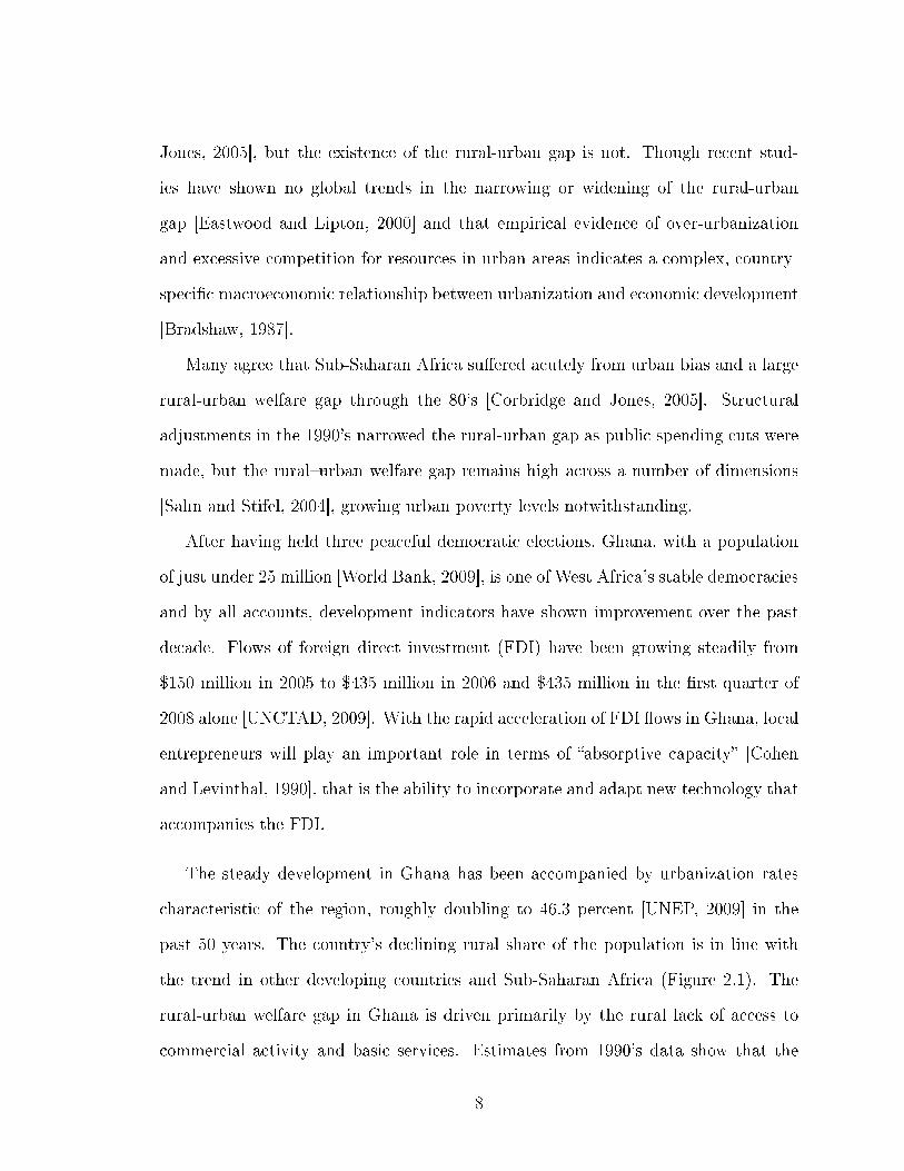
The steady development in Ghana has been accompanied by urbanization rates

characteristic of the region, roughly doubling to 46.3 percent [UNEP, 2009] in the

past 50 years. The country's declining rural share of the population is in line with

the trend in other developing countries and Sub-Saharan Africa (Figure 2.1). The

rural-urban welfare gap in Ghana is driven primarily by the rural lack of access to

commercial activity and basic services. Estimates from 1990's data show that the

8

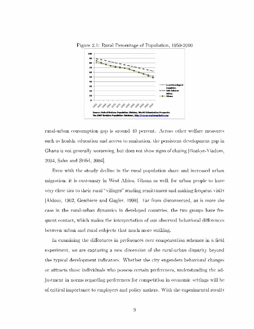
Figure 2.1: Rural Percentage of Population, 1950-2010

rural-urban consumption gap is around 40 percent. Across other welfare measures

such as health, education and access to sanitation, the persistent development gap in

Ghana is not generally worsening, but does not show signs of closing [Boakye-Yiadom,

2004, Sahn and Stifel, 2004].

Even with the steady decline in the rural population share and increased urban

migration, it is customary in West Africa, Ghana as well, for urban people to have

very close ties to their rural �villages� sending remittances and making frequent visits

[Aldous, 1962, Geschiere and Gugler, 1998]. Far from disconnected, as is more the

case in the rural-urban dynamics in developed countries, the two groups have fre-

quent contact, which makes the interpretation of our observed behavioral di�erences

between urban and rural subjects that much more striking.

In examining the di�erences in preferences over compensation schemes in a �eld

experiment, we are capturing a new dimension of the rural-urban disparity beyond

the typical development indicators. Whether the city engenders behavioral changes

or attracts those individuals who possess certain preferences, understanding the ad-

justment in norms regarding preferences for competition in economic settings will be

of critical importance to employers and policy makers. With the experimental results

9

we may be able to examine some endogenous determinants of the �urban bias.�

Despite the increasing urbanization of West Africa in recent decades, much of

the �eld work in Africa continues to concentrate on rural village communities. Our

research generates a rich experimental data set for an under-researched, but very

important and growing demographic group of urban Africans. The results will moti-

vate further study into the causes, costs and bene�ts of preferences for competition

and address broad questions regarding the interrelationship between urbanization and

economic development in Africa.

We used experimental techniques to assess whether rural and urban populations

in Ghana exhibit distinct preferences to engage in a risky, performance-based tourna-

ment in order to identify any di�erences between the groups in some important traits

typically associated with entrepreneurs.

Our experimental data show that when presented with the choice between per-

forming a simple task, 1) for a piece rate wage or 2) in an all-or-nothing tournament,

only 30 percent of the subjects sampled from representative rural and urban areas in

the North and South of Ghana chose to enter the tournament. The tournament entry

percentage was substantially lower than that of similar experiments conducted both

in industrialized countries [Gupta et al., 2005, Niederle and Vesterlund, 2007] and in

traditional cultures in developing countries [Gneezy et al., 2009]. We also identi�ed a

large di�erence in the tournament entry decision between rural and urban subjects:

urban subjects were 20 percent more likely to choose the tournament than their ru-

ral counterparts. We attribute the overall low tournament entry primarily to rural

subjects lower con�dence in terms of relative performance.

Given our motivation, which is to see whether competitive preferences di�er by ru-

ral and urban areas with implications on entrepreneurship and the development of new

business ventures, our experimental design has rural(urban) people competing other

10

rural(urban) people. The within group competition is justi�ed as the entrepreneurs

would be competing locally. This design feature contrasts with the gender and com-

petition studies [Gneezy et al., 2009, Gupta et al., 2005, Niederle and Vesterlund,

2007], where the two groups of interest, men and women, compete within experimen-

tal sessions. The motivation of the gender studies in explaining gender di�erences in

competitive preferences in the workplace supports the mixed gender sessions, where

the interaction between the genders is important in establishing the external validity

of the experiment.

In simulating the entrepreneurial environment with an artefactual experiment,

we present the experimental subjects with a new, unfamiliar and relatively abstract

task, in the sense that the task is being completed for its own sake with no real life

implications. However, the abstract environment may be particularly relevant given

that entrepreneurship frequently involves untested ideas where people may have little

experience. The ability to identify and exploit opportunities and to perform amidst

risk and uncertainty are personal attributes frequently associated with entrepreneurs.

The simple experiments, described in detail in Section 3, were conducted in two

cities, Accra and Tamale and two towns, Nynkapala and Osino in Ghana to establish

a baseline understanding for preferences for competition. In Section 4, we discuss

the developing country �eld setting and identify demographic characteristics of the

subjects. Section 5 provides an analysis of our key �ndings regarding the determinants

of competitive behavior and some of the associated costs. Section 6 concludes with

a discussion regarding the implications of our �ndings on development and proposals

for follow-up experiments to answer any questions that arise from the analysis in

Section 5. The following section provides a summary of related work.

11

2.2 Related Literature

Recent experimental research has used tournament choice to illustrate di�erences

in preferences over competitive situations across cultures, genders and occupations

[Gneezy et al., 2009, Gupta et al., 2005, Niederle and Vesterlund, 2007, Carpenter

and Seki, 2005]. While the experiments elicit preferences over competitive compen-

sation schemes, they also measure attitudes toward con�dence, risk, uncertainty and

performance under pressure. The ability to identify and exploit opportunities and

to perform amidst risk and uncertainty are personal attributes frequently associated

with entrepreneurs in the economics and psychology literature [Kihlstrom and La�ont,

1979].1

Bewley [1989] shows a theoretical link between low uncertainty aversion and busi-

ness innovation in entrepreneurship. In a study of Indian small and medium scale

entrepreneurs, Natarajan [2005] �nds that tolerance for competition is a key char-

acteristic of all of those surveyed. Though certain characteristics of entrepreneurs

may not be robust to cultural comparisons as Thomas and Mueller [2000] demon-

strate empirically, they do �nd that within a given culture certain characteristics can

distinguish the set of entrepreneurs from the rest of the population.

Little theoretical or empirical work has focused explicitly on the characteristics

of developing country entrepreneurs [Le�, 1979, Naude, 2008] who face very di�er-

ent regulatory and credit constraints than their developed country counterparts and

who may potentially di�erent attitudes toward innovation, competition and risk. For

example, Blanch�ower and Oswald [1993] �nd a signi�cant empirical positive link

1 Busenitz [1999] hypothesizes that entrepreneurs are not less risk averse than the general pop-

ulation but their reliance on heuristics and biases may make them appear to be more likely to take

on risk than others.

12

between a lack of capital constraints and a person's status as an entrepreneur; no

such link is found with their measure of psychological characteristics. However, the

context is clearly for that of employed, developed country individuals, with primary

motivations for becoming an entrepreneur being freedom and �exibility. It is clear

that in a given developing country, more will need to be understood regarding the mo-

tivations of local entrepreneurs before we can establish which results from developed

countries are relevant in the developing country context.

In a meta-analysis of entrepreneurship selection, Van der Sluis et al. [2005] �nd the

e�ect of education on worker choice between self-employment and wage employment

stronger in urban areas, the least developed economies and those that are heavily

dependent on agriculture, much like Ghana. In a comprehensive study of Ghanaian

entrepreneurs, Robson et al. [2009] �nd that small and medium scale entrepreneurs

tend toward incremental product development, not large innovation and that the inno-

vativeness of entrepreneurial activities is positively correlated with the entrepreneur's

education level. These �ndings motivated our subject selection which is discussed in

detail in Section 4.

2.3 Experimental Design

The experimental design enabled us to measure preferences for competition while

controlling for performance, con�dence and ambiguity aversion similar to Gupta,

Poulsen and Villeval [2005] and Niederle and Vesterlund [2007]. We use a novel task,

which will enable us to measure the preferences for competition in this developing

country context.

Subjects performed a simple task under a piece rate payment scheme, followed

13

by a tournament round. Subjects were then asked to choose between the piece rate

and the tournament pay before to be applied to the third round of play. No speci�c

skills or training would have favored anyone beyond the general ability to identify

and match. However, successful performance required a combination of ability and

e�ort.

Identi�cation and Matching Task

We designed a task and an environment that would be appropriate for local subjects

and that would facilitate accurate monitoring. In each city, we constructed 8 work

stations to ensure privacy for each subject to simultaneously complete the task. Be-

cause the task was not computerized, we were concerned with achieving uniformity

between subjects. To minimize variation due to monitoring, the same researcher and

a local assistant each monitored 4 subjects.

Upon arrival, we informed the subjects that each subject would receive a 2 cedis

show-up fee and an additional 3 cedis for completing the experiment. After a brief

explanation of the experimental procedure, subjects read and signed consent forms

followed by a brief demonstration. They were informed that they would perform the

task 4 times and would be given speci�c instructions immediately prior to playing.2

We also told them that one of the tasks would be selected at random to determine

their payo� to ensure maximum e�ort in all tasks. At the conclusion of each round,

subjects were shown only their own performance at the conclusion of each task. They

did not know aggregate result.

At his private workstation, each subject was provided with a 1 quart basket con-

taining an identical mixture of familiar objects. Each basket contained 14 uniquely

2Subjects actually performed the identi�cation and matching task 3 times, but we did not informthem of this at the outset.

14

identi�able objects,3 where each unique object was in the mixture at least once (e.g.

magnet) up to 35 times (e.g. pasta), making the total number of objects in each

basket approximately 200. At the beginning of each task round, each subject was

provided with an identical picture of 21 of the objects in the basket placed in a num-

bered linear order.4 Subjects were then given 60 seconds to place the items from their

basket in the order indicated by the picture. At the end of 60 seconds, time was called

and all subjects were required to stand in a holding area while the monitors scored

and cleared each workstation. Scores were calculated based on number of objects

correctly placed according to the numbered sequence in the picture, measuring both

speed and accuracy. Just prior to each task, the speci�c compensation scheme was

explained in detail, both in English and in a local language, where necessary.5

Task 1, Piece Rate: Subjects were given 60 seconds to match as many items in

their basket to the corresponding numbered sequence distributed at the beginning of

the round. If the task was randomly selected, the subject received 50 peswas per item

correctly matched.6

Task 2, Tournament : Subjects were randomly assigned to groups of 4. Subjects

were not told who was in their group, but they were be able to see all of the possible

subjects who could possibly be included in their group. Subjects were then informed

that in the tournament round, payment would based on relative performance within

the randomly assigned group of 4. The highest performing subject in the group

3The objects varied in all dimensions, though most were some form of dried food: Bean (3types), Dried Okra, Eraser, Magnet, Nail, Paper Clip, Pasta (3 types), Plastic Disc, Tamarind Podand Toothpick. Object composition varied between Accra and Tamale as all objects were purchasedlocally. The di�erences between the Accra and Tamale basket composition were minor and cannotaccount for any Accra-Tamale di�erences in performance.

4The number 21 was chosen optimally, after initial testing of the task by the researchers andassistant, to be the lowest number of objects that would guarantee all subjects score below thebound in the 60 second time limit, with some added contingency.

5Instructions are available upon request.6The Ghanaian currency is the cedi, 1.3 cedis = 1 USD. The smallest unit of the currency is the

peswa, 100 peswas = 1 cedi.

15

would receive 2 cedis per correct answer and the others would receive zero. In the

case of a tie, the winner was chosen at random from the high scorers. If each of the

4 competitors has a 25 percent chance of winning, then the tournament payo� is the

same as the piece rate payo�, in expectation.

Task 3, Payment Choice 1 : Subjects were asked before performing the task for

a third time, the choice of payment scheme to be applied to the third round perfor-

mance. They were given the choice between piece rate or tournament pay. For the

tournament choice, individual performance in round 3 was compared to tournament

performance in Task 2. That is to say, individuals who chose the tournament would

not be competing directly with one another in Task 3, but with the outcomes of

Task 2. This was to ensure that the subject's choice to enter the tournament was an

individual choice that did not depend on others choice of tournament entry.

Task 4, Payment Choice 2 : Upon completion of Task 3, subjects were asked

whether they would like to be paid a piece rate or tournament wage for Task 1 perfor-

mance. By giving the subjects the option to submit their past piece rate performance

to the tournament, we have separated the choice of entering into the competition

from the desire to actually perform in a competitive setting.

Beliefs-Assessment Finally, we asked each subject how they believe they ranked,

from 1 (best) to 4 (worst) in Tasks 1 and 2, out of the group of 4 from the Task 2,

tournament round. Subjects were paid 50 peswas per correct identi�cation of rank.

The responses to the questions regarding relative performance enabled us to gage

con�dence and how it relates to the decision to compete.

16

2.4 Field Settings and Subject Selection

The importance of �eld experiments for questions regarding preferences for compe-

tition should be clear given the strong cultural components that surround the way

people compete in the marketplace. Because of the high inequality in Ghana, we risk

too many confounding factors from education to income to levels of outside exposure

would preclude our ability to attribute observed behavioral di�erences between sub-

jects to �urban� or �rural�. As a result, we selected subjects with relatively similar

demographic characteristics such as age, education and income across the rural and

urban areas. Because of the critical importance of development through the formal

sector, the subject pool in our experiments was limited to current and potential for-

mal sector workers; all subjects were literate and had experience with modernized

non-physical labor either through secondary school or their current occupation. In

addition, the working-class segment of the population, from which we drew our sub-

jects, comprises a large group of unemployed and underemployed citizens whose labor

prospects are closely connected to Ghana's development goals.

To identify and recruit the targeted subject pool, we hired recruiters in each

experimental loaction. The recruiters were local residents who worked with foreign-

based NGO's and who had experience recruiting community members for similar

incentivized activities. The subjects that were selected, by and large, knew each

other with the exception of Accra, where subjects were not familiar with one another.

The �eld experiments were conducted in four locations in rural and urban munici-

palities in the north and south. Ghana, like many of the countries in West Africa, has

a clear social and cultural distinction between the coastal, predominantly Christian

south and the Sahelian predominantly Muslim North.7 To ensure that our experi-

7There are 10 regions in Ghana: Ashanti, Brong Ahafo, Central, Eastern, Greater Accra, North-ern, Upper East, Upper West, Volta and Western.

17

mental subjects adequately represented the North-South divide and some of the other

regional divisions, we conducted the urban experiments in the southern coastal capital

city, Accra and the northern city of Tamale and the rural experiments in the southern

town of Osino and a town outside of Tamale, Nyankapala.8 Accra and the inland city

of Kumasi are the two largest cities in Ghana with 1.7 and 1.2 million inhabitants.

Tamale is distant third with 0.2 million inhabitants. We weighted the sample size

from each region in order to re�ect the actual population distribution.9 We were able

to determine the subject's home region from the short questionnaire administered

after all experimental tasks were completed. Also, as our design is geared toward

addressing entrepreneurship issues, it was important to have a representative cross

section of the Ghanaian population to add to the generalizability of our conclusions.

Subject selection was motivated by actual labor force composition so as to draw

inferences on the current and future labor force characteristics from our experimental

results (Table 2.1). Our recruiting e�orts targeted educated members of the for-

mal sector work force and potential formal sector workers given our motivation of

transformative entrepreneurship and the positive empirical link between innovative-

ness and education found in Ghanaian entrepreneurs [Robson et al., 2009]. With the

help of our local assistants, we recruited subjects at post-secondary schools and area

businesses.

The mean age of the subjects was 24. Rural subjects were slightly younger (23) on

average than urban (25) subjects. All of the subjects were educated with 90 percent

8While nearly all of the subjects in the Accra experiments hailed from the Greater Accra Region,the Tamale subjects were from the Northern Region, including the capital city of Tamale, UpperEast and Upper West.

9Approximately 70 percent of the population lives in the regions constituting the �South,� in-cluding the capital city of Accra and the Ashanti capital Kumasi.

18

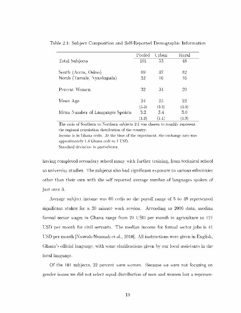
Table 2.1: Subject Composition and Self-Reported Demographic Information

Pooled Urban RuralTotal Subjects 101 53 48

South (Accra, Osino) 69 37 32North (Tamale, Nyankapala) 32 16 16

Percent Women 32 34 29

Mean Age 24 25 23(5.3) (5.3) (5.2)

Mean Number of Languages Spoken 3.2 3.4 3.0(1.2) (1.1) (1.3)

The ratio of Southern to Northern subjects 2:1 was chosen to roughly represent

the regional population distribution of the country.

Income is in Ghana cedis. At the time of the experiment, the exchange rate was

approximately 1.4 Ghana cedi to 1 USD.

Standard deviation in parentheses.

having completed secondary school many with further training, from technical school

to university studies. The subjects also had signi�cant exposure to various ethnicities

other than their own with the self reported average number of languages spoken of

just over 3.

Average subject income was 60 cedis so the payo� range of 5 to 48 represented

signi�cant stakes for a 30 minute work session. According to 2006 data, median

formal sector wages in Ghana range from 21 USD per month in agriculture to 121

USD per month for civil servants. The median income for formal sector jobs is 41

USD per month [Nsowah-Nuamah et al., 2010]. All instructions were given in English,

Ghana's o�cial language, with some clari�cations given by our local assistants in the

local language.

Of the 101 subjects, 32 percent were women. Because we were not focusing on

gender issues we did not select equal distribution of men and women but a represen-

19

tative sample of the pool of potential and current workers. The gender balance of our

subjects re�ected the actual formal sector labor force participation by gender. While

women dominate the informal sector jobs in Ghana, they are outnumbered by men

2:1 in the formal sector.

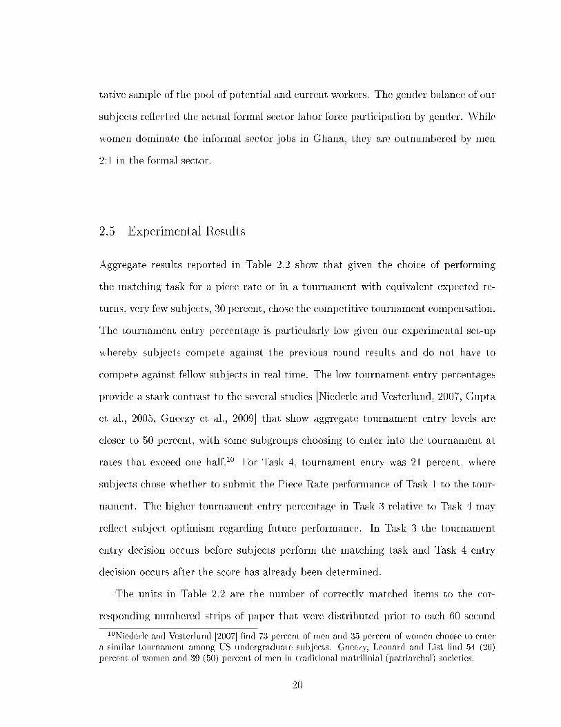
2.5 Experimental Results

Aggregate results reported in Table 2.2 show that given the choice of performing

the matching task for a piece rate or in a tournament with equivalent expected re-

turns, very few subjects, 30 percent, chose the competitive tournament compensation.

The tournament entry percentage is particularly low given our experimental set-up

whereby subjects compete against the previous round results and do not have to

compete against fellow subjects in real time. The low tournament entry percentages

provide a stark contrast to the several studies [Niederle and Vesterlund, 2007, Gupta

et al., 2005, Gneezy et al., 2009] that show aggregate tournament entry levels are

closer to 50 percent, with some subgroups choosing to enter into the tournament at

rates that exceed one half.10 For Task 4, tournament entry was 21 percent, where

subjects chose whether to submit the Piece Rate performance of Task 1 to the tour-

nament. The higher tournament entry percentage in Task 3 relative to Task 4 may

re�ect subject optimism regarding future performance. In Task 3 the tournament

entry decision occurs before subjects perform the matching task and Task 4 entry

decision occurs after the score has already been determined.

The units in Table 2.2 are the number of correctly matched items to the cor-

responding numbered strips of paper that were distributed prior to each 60 second

10Niederle and Vesterlund [2007] �nd 73 percent of men and 35 percent of women choose to entera similar tournament among US undergraduate subjects. Gneezy, Leonard and List �nd 54 (26)percent of women and 39 (50) percent of men in traditional matrilinial (patriarchal) societies.

20

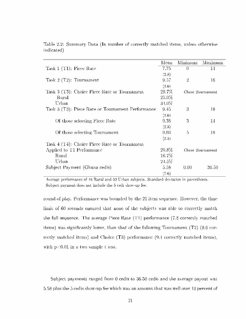
Table 2.2: Summary Data (In number of correctly matched items, unless otherwiseindicated)

Mean Minimum MaximumTask 1 (T1): Piece Rate 7.75 0 14

(2.8)

Task 2 (T2): Tournament 9.57 2 16(2.6)

Task 3 (T3): Choice Piece Rate or Tournament 29.7% Chose Tournament

Rural 25.0%Urban 34.0%

Task 3 (T3): Piece Rate or Tournament Performance 9.45 3 18(2.6)

Of those selecting Piece Rate 9.38 3 14(2.5)

Of those selecting Tournament 9.60 5 18(2.5)

Task 4 (T4): Choice Piece Rate or TournamentApplied to T1 Performance 20.8% Chose Tournament

Rural 16.7%Urban 24.5%

Subject Payment (Ghana cedis) 5.58 0.00 36.50(7.6)

Average performance of 48 Rural and 53 Urban subjects. Standard deviation in parentheses.

Subject payment does not include the 5 cedi show-up fee.

round of play. Performance was bounded by the 21 item sequence. However, the time

limit of 60 seconds ensured that none of the subjects was able to correctly match

the full sequence. The average Piece Rate (T1) performance (7.8 correctly matched

items) was signi�cantly lower, than that of the following Tournament (T2) (9.6 cor-

rectly matched items) and Choice (T3) performance (9.4 correctly matched items),

with p<0.01 in a two sample t test.

Subject payments ranged from 0 cedis to 36.50 cedis and the average payout was

5.58 plus the 5 cedis show-up fee which was an amount that was well over 10 percent of

21

Figure 2.2: Cumulative Density Function, Tasks 1 and 2 by Rural and Urban

�

���

���

���

���

�

� � �� ��

������������ ������

��

�����

�

���

���

���

���

�

� � �� �� ��

�������������� ��������

��

�����

average subject in our sample's monthly income. The maximum number of correctly

matched items in Tasks 1, 2 and 3 were 14, 16 and 18, which is important as all were

below the maximum 21 items in the numbered sequence.

The average Piece Rate performance in the urban group, 8.1, was higher than

the performance in the rural group, 7.4, though this di�erence was not signi�cant (p

= 0.173, Mann-Whitney test). Similarly in the Tournament the urban group mean

score 10.0, was higher than the rural score of 9.1, though the test with p=0.077. The

di�erence in average performance persisted through the �nal round (p = 0.058), Task

3 with average for the urban subjects was 9.9 and for the rural subjects, 8.9. Because

the experimental design did not have any between site interaction and because our

results do not support within site di�erences in performances based on gender, income

or ethnicity (hometown, languages), over the course of our analysis we have controlled

for the di�erences in performance due to experimental location.

22

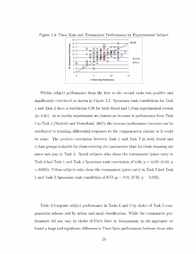
Figure 2.3: Piece Rate and Tournament Performance by Experimental Subject

���������������

� � �� ��

�������

���

����

� ��

���

���������������� �����

���

���

�����

Within subject performance from the �rst to the second tasks was positive and

signi�cantly correlated as shown in Figure 2.3. Spearman rank correlations for Task

1 and Task 2 show a correlation 0.38 for both Rural and Urban experimental session

(p<0.01). As in similar experiments we observe an increase in performance from Task

1 to Task 2 (Niederle and Vesterlund, 2007); the increase performance increase can be

attributed to learning, di�erential responses to the compensation scheme or it could

be noise. The positive correlation between Task 1 and Task 2 in both Rural and

Urban groups is double for those entering the tournament than for those choosing the

piece rate pay in Task 3. Rural subjects who chose the tournament (piece rate) in

Task 3 had Task 1 and Task 2 Spearman rank correlation of 0.60, p = 0.041 (0.33, p

= 0.050). Urban subjects who chose the tournament (piece rate) in Task 3 had Task

1 and Task 2 Spearman rank correlation of 0.73, p < 0.01 (0.32, p = 0.062).

Table 2.3 reports subject performance in Tasks 1 and 2 by choice of Task 3 com-

pensation scheme and by urban and rural classi�cation. While the tournament per-

formance did not vary by choice of Piece Rate or Tournament, in the aggregate we

found a large and signi�cant di�erence in Piece Rate performance between those who

23

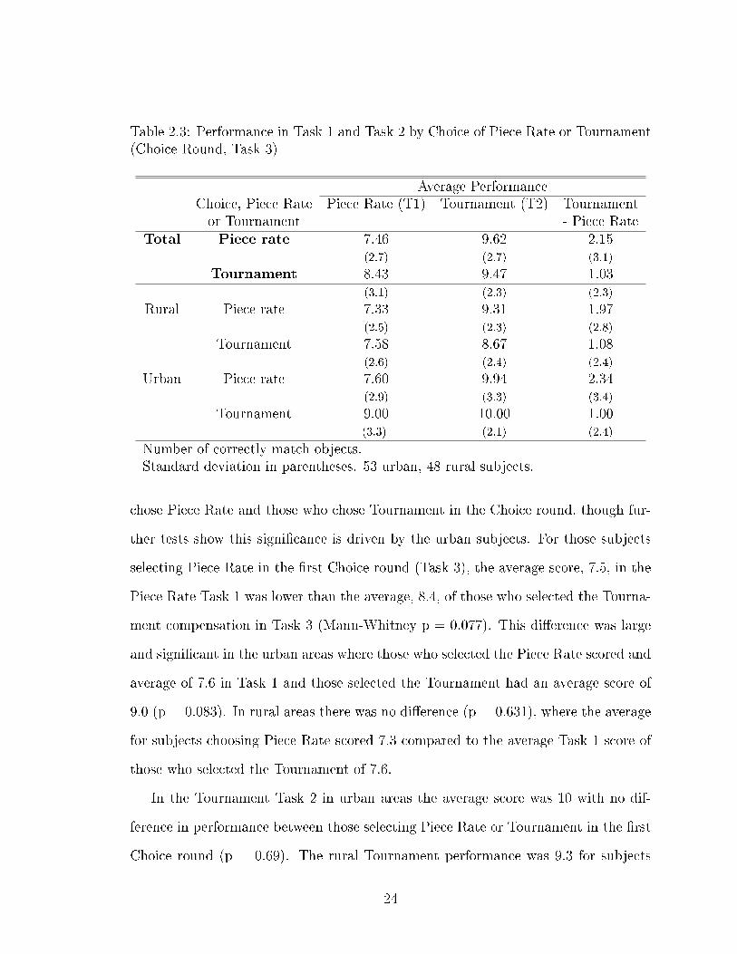
Table 2.3: Performance in Task 1 and Task 2 by Choice of Piece Rate or Tournament(Choice Round, Task 3)

Average PerformanceChoice, Piece Rate Piece Rate (T1) Tournament (T2) Tournamentor Tournament - Piece Rate

Total Piece rate 7.46 9.62 2.15(2.7) (2.7) (3.1)

Tournament 8.43 9.47 1.03(3.1) (2.3) (2.3)

Rural Piece rate 7.33 9.31 1.97(2.5) (2.3) (2.8)

Tournament 7.58 8.67 1.08(2.6) (2.4) (2.4)

Urban Piece rate 7.60 9.94 2.34(2.9) (3.3) (3.4)

Tournament 9.00 10.00 1.00(3.3) (2.1) (2.4)

Number of correctly match objects.Standard deviation in parentheses. 53 urban, 48 rural subjects.

chose Piece Rate and those who chose Tournament in the Choice round, though fur-

ther tests show this signi�cance is driven by the urban subjects. For those subjects

selecting Piece Rate in the �rst Choice round (Task 3), the average score, 7.5, in the

Piece Rate Task 1 was lower than the average, 8.4, of those who selected the Tourna-

ment compensation in Task 3 (Mann-Whitney p = 0.077). This di�erence was large

and signi�cant in the urban areas where those who selected the Piece Rate scored and

average of 7.6 in Task 1 and those selected the Tournament had an average score of

9.0 (p = 0.083). In rural areas there was no di�erence (p = 0.631), where the average

for subjects choosing Piece Rate scored 7.3 compared to the average Task 1 score of

those who selected the Tournament of 7.6.

In the Tournament Task 2 in urban areas the average score was 10 with no dif-

ference in performance between those selecting Piece Rate or Tournament in the �rst

Choice round (p = 0.69). The rural Tournament performance was 9.3 for subjects

24

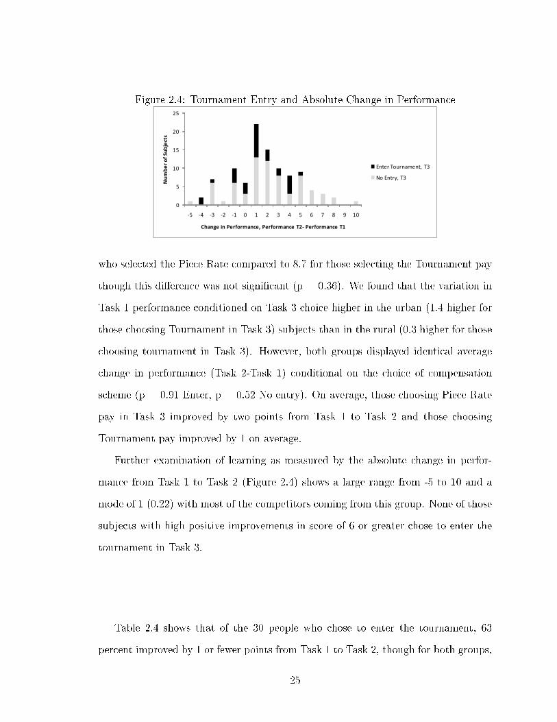
Figure 2.4: Tournament Entry and Absolute Change in Performance

�

�

��

��

��

��

�� �� �� �� �� � � � � � � � � ��

����

������

���� �

������������� ��������� �������� ��� �������

� �������� ��� ��� ������ �������

who selected the Piece Rate compared to 8.7 for those selecting the Tournament pay

though this di�erence was not signi�cant (p = 0.36). We found that the variation in

Task 1 performance conditioned on Task 3 choice higher in the urban (1.4 higher for

those choosing Tournament in Task 3) subjects than in the rural (0.3 higher for those

choosing tournament in Task 3). However, both groups displayed identical average

change in performance (Task 2-Task 1) conditional on the choice of compensation

scheme (p = 0.91 Enter, p = 0.52 No entry). On average, those choosing Piece Rate

pay in Task 3 improved by two points from Task 1 to Task 2 and those choosing

Tournament pay improved by 1 on average.

Further examination of learning as measured by the absolute change in perfor-

mance from Task 1 to Task 2 (Figure 2.4) shows a large range from -5 to 10 and a

mode of 1 (0.22) with most of the competitors coming from this group. None of those

subjects with high positive improvements in score of 6 or greater chose to enter the

tournament in Task 3.

Table 2.4 shows that of the 30 people who chose to enter the tournament, 63

percent improved by 1 or fewer points from Task 1 to Task 2, though for both groups,

25

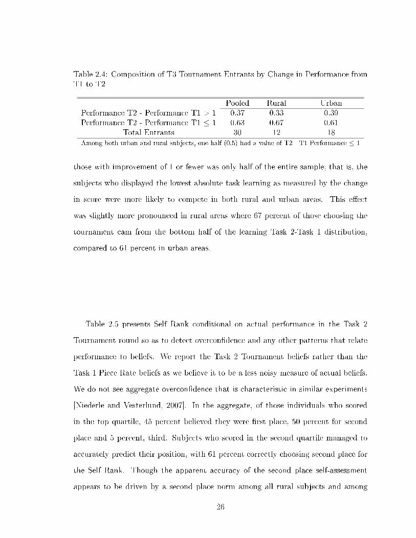
Table 2.4: Composition of T3 Tournament Entrants by Change in Performance fromT1 to T2

Pooled Rural UrbanPerformance T2 - Performance T1 > 1 0.37 0.33 0.39Performance T2 - Performance T1 ≤ 1 0.63 0.67 0.61

Total Entrants 30 12 18Among both urban and rural subjects, one half (0.5) had a value of T2 - T1 Performance ≤ 1

those with improvement of 1 or fewer was only half of the entire sample; that is, the

subjects who displayed the lowest absolute task learning as measured by the change

in score were more likely to compete in both rural and urban areas. This e�ect

was slightly more pronounced in rural areas where 67 percent of those choosing the

tournament cam from the bottom half of the learning Task 2-Task 1 distribution,

compared to 61 percent in urban areas.

Table 2.5 presents Self Rank conditional on actual performance in the Task 2

Tournament round so as to detect overcon�dence and any other patterns that relate

performance to beliefs. We report the Task 2 Tournament beliefs rather than the

Task 1 Piece Rate beliefs as we believe it to be a less noisy measure of actual beliefs.

We do not see aggregate overcon�dence that is characteristic in similar experiments

[Niederle and Vesterlund, 2007]. In the aggregate, of those individuals who scored

in the top quartile, 45 percent believed they were �rst place, 50 percent for second

place and 5 percent, third. Subjects who scored in the second quartile managed to

accurately predict their position, with 61 percent correctly choosing second place for

the Self Rank. Though the apparent accuracy of the second place self-assessment

appears to be driven by a second place norm among all rural subjects and among

26

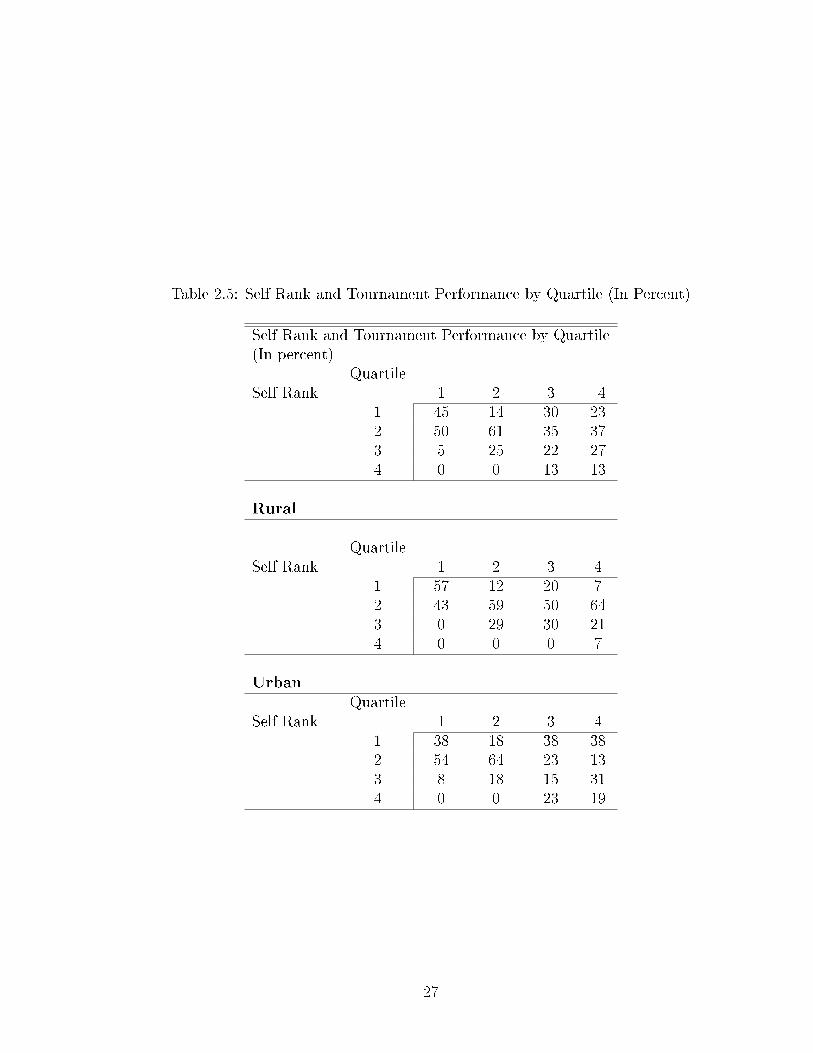
Table 2.5: Self Rank and Tournament Performance by Quartile (In Percent)

Self Rank and Tournament Performance by Quartile(In percent)

QuartileSelf Rank 1 2 3 4

1 45 14 30 232 50 61 35 373 5 25 22 274 0 0 13 13

Rural

QuartileSelf Rank 1 2 3 4

1 57 12 20 72 43 59 50 643 0 29 30 214 0 0 0 7

UrbanQuartile

Self Rank 1 2 3 41 38 18 38 382 54 64 23 133 8 18 15 314 0 0 23 19

27

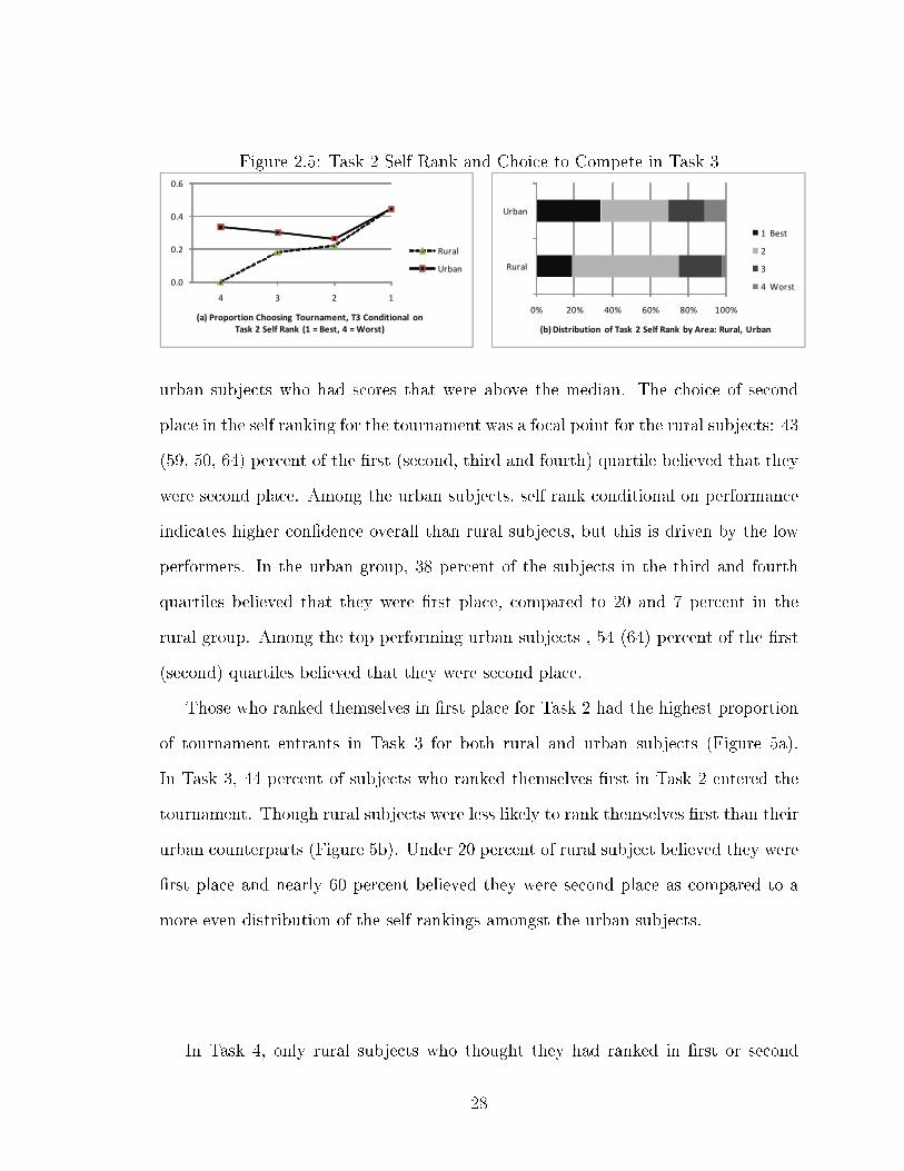
Figure 2.5: Task 2 Self Rank and Choice to Compete in Task 3

���

���

���

���

����

�������������� ������ ����������������������� ��������������������� ���������� ���!����

���

���

�� ��� ��� ��� ��� ����

���

���

�"��#��"���� �������� ������������ "$�%���&�������� '�"��

�������

�

�

�������

urban subjects who had scores that were above the median. The choice of second

place in the self ranking for the tournament was a focal point for the rural subjects: 43

(59, 50, 64) percent of the �rst (second, third and fourth) quartile believed that they

were second place. Among the urban subjects, self rank conditional on performance

indicates higher con�dence overall than rural subjects, but this is driven by the low

performers. In the urban group, 38 percent of the subjects in the third and fourth

quartiles believed that they were �rst place, compared to 20 and 7 percent in the

rural group. Among the top performing urban subjects , 54 (64) percent of the �rst

(second) quartiles believed that they were second place.

Those who ranked themselves in �rst place for Task 2 had the highest proportion

of tournament entrants in Task 3 for both rural and urban subjects (Figure 5a).

In Task 3, 44 percent of subjects who ranked themselves �rst in Task 2 entered the

tournament. Though rural subjects were less likely to rank themselves �rst than their

urban counterparts (Figure 5b). Under 20 percent of rural subject believed they were

�rst place and nearly 60 percent believed they were second place as compared to a

more even distribution of the self rankings amongst the urban subjects.

In Task 4, only rural subjects who thought they had ranked in �rst or second

28

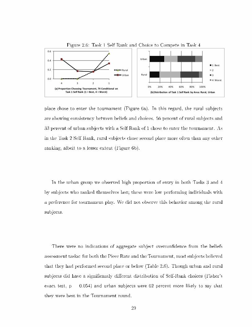
Figure 2.6: Task 1 Self Rank and Choice to Compete in Task 4

���

���

���

���

����

�������������� ������ ����������������������� ��������������������� �������������������

���

���

�� ��� ��� ��� ��� ����

���

���

� ��!�� ���� �������� ������������ "�#���$�������� %� ��

�������

�

�

�������

place chose to enter the tournament (Figure 6a). In this regard, the rural subjects

are showing consistency between beliefs and choices. 56 percent of rural subjects and

33 percent of urban subjects with a Self Rank of 1 chose to enter the tournament. As

in the Task 2 Self Rank, rural subjects chose second place more often than any other

ranking, albeit to a lesser extent (Figure 6b).

In the urban group we observed high proportion of entry in both Tasks 3 and 4

by subjects who ranked themselves last; these were low performing individuals with

a preference for tournament play. We did not observe this behavior among the rural

subjects.

There were no indications of aggregate subject overcon�dence from the beliefs

assessment tasks: for both the Piece Rate and the Tournament, most subjects believed

that they had performed second place or below (Table 2.6). Though urban and rural

subjects did have a signi�cantly di�erent distribution of Self-Rank choices (Fisher's

exact test, p = 0.054) and urban subjects were 62 percent more likely to say that

they were best in the Tournament round.

29

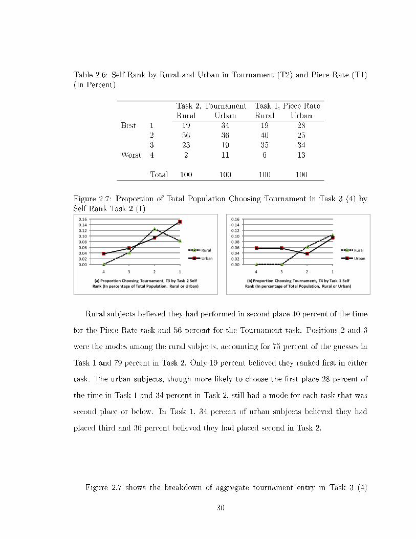
Table 2.6: Self Rank by Rural and Urban in Tournament (T2) and Piece Rate (T1)(In Percent)

Task 2, Tournament Task 1, Piece RateRural Urban Rural Urban

Best 1 19 34 19 282 56 36 40 253 23 19 35 34

Worst 4 2 11 6 13

Total 100 100 100 100

Figure 2.7: Proportion of Total Population Choosing Tournament in Task 3 (4) bySelf Rank Task 2 (1)

������������������������������������

����

�������������� ������ ���������������������� �������������������������������������������� ��������� �����

��

�����������������������������������������

����

�������������� ����������������� �!��������� "������������������������������������������� ��������� �����

��

�����

Rural subjects believed they had performed in second place 40 percent of the time

for the Piece Rate task and 56 percent for the Tournament task. Positions 2 and 3

were the modes among the rural subjects, accounting for 75 percent of the guesses in

Task 1 and 79 percent in Task 2. Only 19 percent believed they ranked �rst in either

task. The urban subjects, though more likely to choose the �rst place 28 percent of

the time in Task 1 and 34 percent in Task 2, still had a mode for each task that was

second place or below. In Task 1, 34 percent of urban subjects believed they had

placed third and 36 percent believed they had placed second in Task 2.

Figure 2.7 shows the breakdown of aggregate tournament entry in Task 3 (4)

30

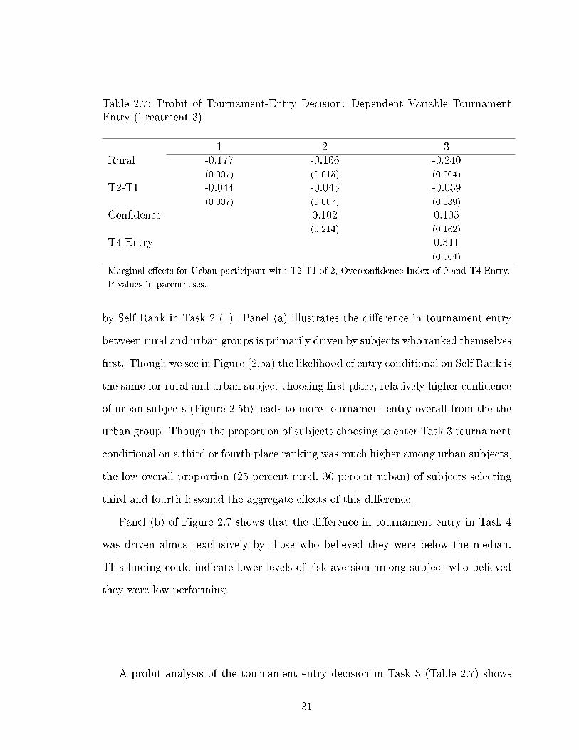
Table 2.7: Probit of Tournament-Entry Decision: Dependent Variable TournamentEntry (Treatment 3)

1 2 3Rural -0.177 -0.166 -0.240

(0.007) (0.015) (0.004)

T2-T1 -0.044 -0.045 -0.039(0.007) (0.007) (0.039)

Con�dence 0.102 0.105(0.214) (0.162)

T4 Entry 0.311(0.004)

Marginal e�ects for Urban participant with T2-T1 of 2, Overcon�dence Index of 0 and T4 Entry.

P values in parentheses.

by Self Rank in Task 2 (1). Panel (a) illustrates the di�erence in tournament entry

between rural and urban groups is primarily driven by subjects who ranked themselves

�rst. Though we see in Figure (2.5a) the likelihood of entry conditional on Self Rank is

the same for rural and urban subject choosing �rst place, relatively higher con�dence

of urban subjects (Figure 2.5b) leads to more tournament entry overall from the the

urban group. Though the proportion of subjects choosing to enter Task 3 tournament

conditional on a third or fourth place ranking was much higher among urban subjects,

the low overall proportion (25 percent rural, 30 percent urban) of subjects selecting

third and fourth lessened the aggregate e�ects of this di�erence.

Panel (b) of Figure 2.7 shows that the di�erence in tournament entry in Task 4

was driven almost exclusively by those who believed they were below the median.

This �nding could indicate lower levels of risk aversion among subject who believed

they were low performing.

A probit analysis of the tournament entry decision in Task 3 (Table 2.7) shows

31

the marginal e�ects of being rural, absolute change in performance, con�dence and

tournament entry in Task 4 for an urban subject with a change in score of 2, a

Con�dence Index value of 0 in Task 2 and who entered the tournament in Task

4.11 Regression 1 shows rural subjects were 17.7 percentage points (p < 0.01) less

likely to enter the tournament given their change in performance. The marginal

e�ects of the absolute change in performance, -0.044 (p < 0.01) show subjects were

less likely to enter the tournament the more they improved from Task 1 to Task 2.

When we include the Con�dence Index in Regression 2, we �nd a positive marginal

e�ect of having more con�dence, but this result is not signi�cant (p = 0.21). The

lack of signi�cance on the con�dence term should not be surprising as even if a

subject is measured overcon�dent, unless he thinks he was �rst place, entering the

tournament is not a rational choice. The high selection of 2nd and 3rd place by rural

and urban subjects is preventing the data for the self-rank measure from being a

determinant of tournament entry. The magnitude and signi�cance of the coe�cients

on the rural dummy and change in performance are essentially unchanged with the

addition of the con�dence variable. Regression 3 includes the decision to enter into

the tournament in the 4th round, which can be considered a measure of preferences

for competitive institutions isolated from preferences to actually compete. The Task

4 entry variable is positive and signi�cant (p < 0.01), and the marginal e�ects of the

11 The measure of con�dence re�ects the distance between guessed and actual rank, weighted

by their actual rank, (Actual Rank-Self Rank)/Actual Rank. This construction of the measure of

con�dence weights undercon�dence heavily, that is, where subjects guessed that they were in a lower

position than they actually were. The possible values ranged from -3 to 0.75, but for both Task 1 and

Task 2, the range was -2 to 0.75. Subjects were slightly less con�dent in their Task 1 performance

with average index value of -0.14 compared to the Task 2 average, -0.12, though this di�erence was

not signi�cant (two-sample t-test, p = 0.878).

32

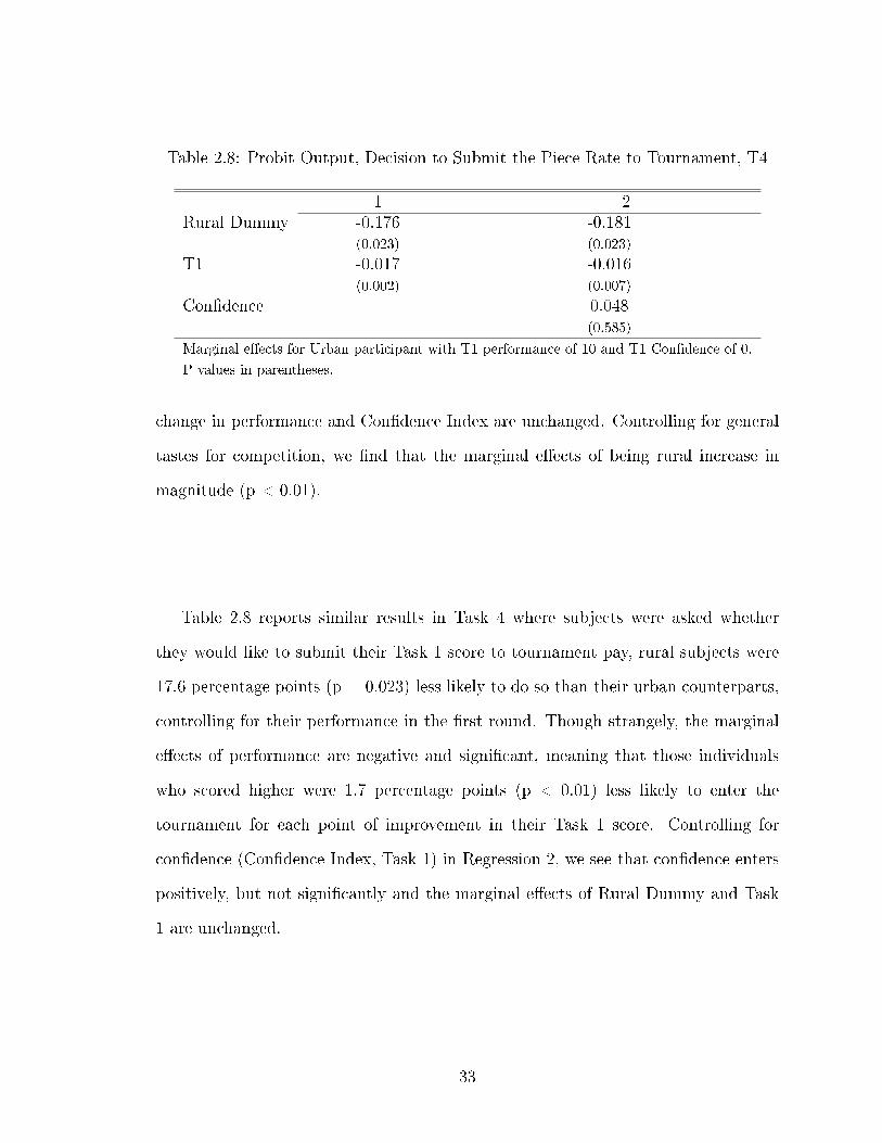
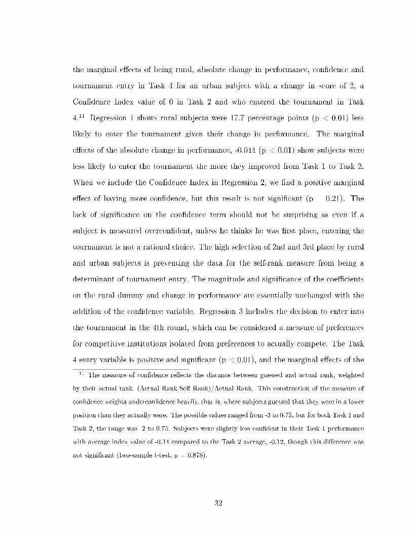
Table 2.8: Probit Output, Decision to Submit the Piece Rate to Tournament, T4

1 2Rural Dummy -0.176 -0.181

(0.023) (0.023)

T1 -0.017 -0.016(0.002) (0.007)

Con�dence 0.048(0.585)

Marginal e�ects for Urban participant with T1 performance of 10 and T1 Con�dence of 0.

P values in parentheses.

change in performance and Con�dence Index are unchanged. Controlling for general

tastes for competition, we �nd that the marginal e�ects of being rural increase in

magnitude (p < 0.01).

Table 2.8 reports similar results in Task 4 where subjects were asked whether

they would like to submit their Task 1 score to tournament pay, rural subjects were

17.6 percentage points (p = 0.023) less likely to do so than their urban counterparts,

controlling for their performance in the �rst round. Though strangely, the marginal

e�ects of performance are negative and signi�cant, meaning that those individuals

who scored higher were 1.7 percentage points (p < 0.01) less likely to enter the

tournament for each point of improvement in their Task 1 score. Controlling for

con�dence (Con�dence Index, Task 1) in Regression 2, we see that con�dence enters

positively, but not signi�cantly and the marginal e�ects of Rural Dummy and Task

1 are unchanged.

33

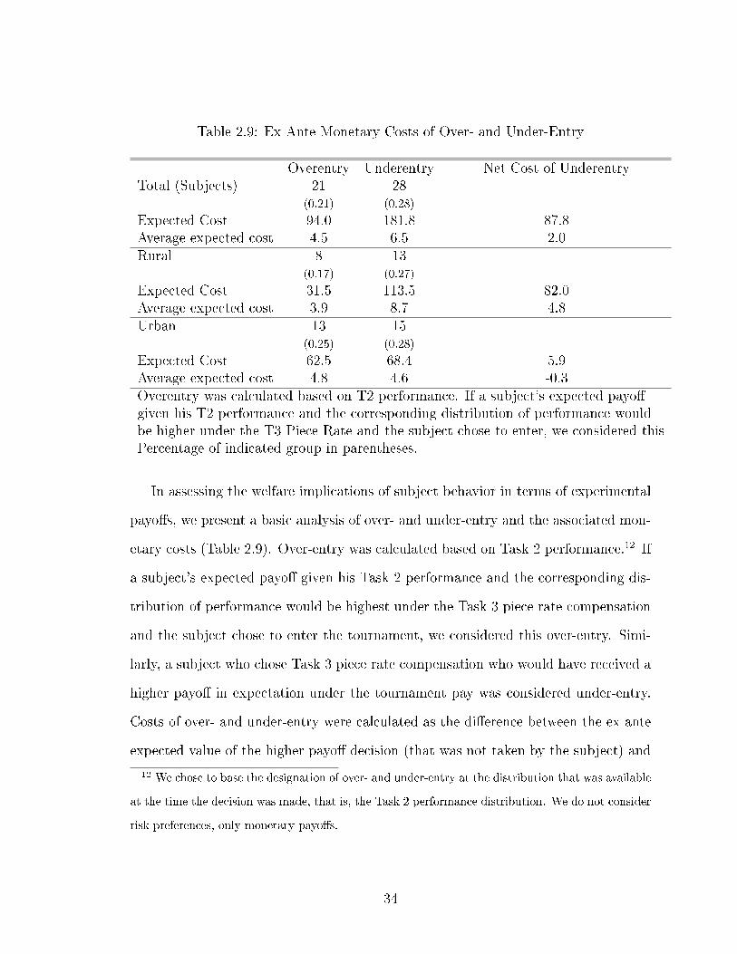
Table 2.9: Ex Ante Monetary Costs of Over- and Under-Entry

Overentry Underentry Net Cost of UnderentryTotal (Subjects) 21 28

(0.21) (0.28)

Expected Cost 94.0 181.8 87.8Average expected cost 4.5 6.5 2.0Rural 8 13

(0.17) (0.27)

Expected Cost 31.5 113.5 82.0Average expected cost 3.9 8.7 4.8Urban 13 15

(0.25) (0.28)

Expected Cost 62.5 68.4 5.9Average expected cost 4.8 4.6 -0.3Overentry was calculated based on T2 performance. If a subject's expected payo�given his T2 performance and the corresponding distribution of performance wouldbe higher under the T3 Piece Rate and the subject chose to enter, we considered thisPercentage of indicated group in parentheses.

In assessing the welfare implications of subject behavior in terms of experimental

payo�s, we present a basic analysis of over- and under-entry and the associated mon-

etary costs (Table 2.9). Over-entry was calculated based on Task 2 performance.12 If

a subject's expected payo� given his Task 2 performance and the corresponding dis-

tribution of performance would be highest under the Task 3 piece rate compensation

and the subject chose to enter the tournament, we considered this over-entry. Simi-

larly, a subject who chose Task 3 piece rate compensation who would have received a

higher payo� in expectation under the tournament pay was considered under-entry.

Costs of over- and under-entry were calculated as the di�erence between the ex ante

expected value of the higher payo� decision (that was not taken by the subject) and

12 We chose to base the designation of over- and under-entry at the distribution that was available

at the time the decision was made, that is, the Task 2 performance distribution. We do not consider

risk preferences, only monetary payo�s.

34

the payo� given the actual choice. While both rural and urban had under-entry rates

of 0.3, over-entry was less common in rural groups, 0.17, compared to urban, 0.25.

The expected costs of under-entry were higher than the costs for over-entry in both

groups, though only signi�cantly so in the rural case where on average, net under-

entry (cost of under-entry-cost of over-entry) cost each subject 4.8 cedis, the show-up

fee. Urban subjects did not systematically over- or under-enter and the net cost of

under-entry was essentially zero.

2.6 Discussion and Conclusion

Our results indicate a general preference for a non-competitive compensation scheme

over a competitive of both urban and rural subjects in artefactual �eld experiments.

However, urban subjects were around 20 percent more likely to enter into the tourna-

ment than were their rural counterparts. Our analysis points to ambiguity aversion

as the primary driver of the observed behavior and for the rural-urban di�erence in

tournament entry. Though all subjects indicated di�culty assessing relative ability in

new tasks, the urban subjects were overall more comfortable with uncertainty when

the potential rewards were high.

While the task in our experiment is simple and requires no special training or skill

to be successful, subjects appeared to feel pressure by the time constraint thereby

making what would otherwise be a trivially easy task di�cult. In fact, no subject

was able to complete the task (correctly �ll all 21 bins) and the highest score of 18

was earned by a single subject. The di�culty of the task is a likely factor in the

observed low con�dence, which is consistent with the �ndings that people tend to

believe they are performing better than average on easy tasks and worse on di�cult

35

ones [Moore and Small, 2007]. When we reduced the uncertainty in a set of pilot

experiments by announcing the score to beat to the rural subjects, participation on

the tournament doubled. This supports the hypothesis that ambiguity aversion over

risk aversion kept subjects from participating in the tournament in prior rounds.

Though the urban subjects did tend to perform better than the rural ones, because

we did not have and between group comparison, this should not have played any role

in the rural subjects willingness to select the tournament. However, we detected one

fundamental di�erence between the two groups with regards to the Beliefs Assessment.

Irrespective of actual performance, rural subjects were most likely to guess that they

were in second place and we did not observe the same selection of second place for the

urban subjects. Conditional upon that belief of second place, there was no di�erence

in tournament entry between urban and rural groups. However, urban subjects were

much more likely to think that they were �rst place and thus entered more often.

Also, the urban subjects had a group of risk takers who thought they were in third

and fourth place and still chose to enter the tournament in the Choice rounds.

As the demographic characteristics of the subjects is otherwise identical between

the rural and urban, it makes our �ndings that much more striking with implications

that support to a widely held view that rural people are less competitive than urban

people, even when controlling for a battery of demographic traits such as age, income

and gender. With the emergence of programs government run and civil society to

promote entrepreneurship in Ghana, it will be of critical importance for those design-

ing the programs to understand the cultural predispositions of the pool of potential

entrepreneurs and whether urban areas stand to receive a disproportionately higher

bene�t than rural areas due to systematic behavioral characteristics, such as stronger

preferences for competition amidst uncertainty.

While our study does not address urban-rural migration, using recent immigrant

36

subjects, we can use a similar experimental design to test whether competitiveness of

rural immigrants is systematically di�erent from those who do not choose to move to

the city. The out-migration of competitive individuals from rural areas has implica-

tions on the quantity and types of business activities that are locally developed and

sustained.

The strong signi�cant relationship between the change in score from the Piece

Rate to the Tournament rounds indicated that subjects were less likely to enter the

Tournament if they showed more improvement. If past performance was the subject's

primary input as he calculated the expected performance, then it would follow that

higher variance in the score would mean lower expected performance in relation to

the top score. The further the expected performance was from the top score, the less

likely a subject would assess themselves as being able to score in �rst place and thus

enter the tournament. The uncertainty that each subject had regarding the top score

caused subjects to overweight the probability of scoring low in subsequent rounds.

With potential payo�s representing at least 10 percent of a month's wages for a

typical worker, �nancial incentives were su�ciently high in both the Piece Rate and

Tournament compensation schemes to induce high levels of concentration and e�ort

in all tasks. However, our data are consistent with �ndings in the literature that rank-

order tournament incentive schemes induce higher e�ort than piece rates [Lazear and

Rosen, 1981, Bull et al., 1987]. Preliminary �ndings in a task where subjects learn the

top score (that must be exceeded) indicate that there is an interaction between not

only the choice to enter the tournament, which increased with increased information,

but with e�ort levels as well, which also increase.

In contrast to the related literature that evaluates preferences for competition

with heterogeneous group composition (men and women) [Gupta et al., 2005, Gneezy

et al., 2009, Niederle and Vesterlund, 2007], our experimental design consisted of

37

homogeneous groups, similar to Carpenter and Seki [2005], which freed us from having

to consider any between group interactions that may have a�ected our measurement

of preferences.

Higher performing individuals were disproportionately less con�dent than their

lower performing counterparts, which helps to explain the overall low tournament

entry. The propensity of the high performing subjects to shy away from the high risk-

high return tournament compensation may re�ect the environment where scarcity

of good jobs implies a high opportunity cost of forgoing a good job to become an

entrepreneur. Higher performing individuals have more to lose from entering the

tournament and losing than do the low performing individuals. Trends in quartile

performance graph may re�ect this counter-intuitive trend that occurred with both

rural and urban subjects.

To fully capture the implications of our �ndings on the potential for growth in

entrepreneurship in rural and urban areas, it will be important to compare the results

from these artefactual experiments with results from similar �eld experiments with

local entrepreneurs. Though even without comparison, the subjects' display of a

strong lack of con�dence in an unfamiliar setting is likely an indicator of people's

adverse attitude toward seeking out opportunities when a safe option is available. If

the only entrepreneurs in the society are very small-scale and doing so out of necessity,

as opposed to those who have a relatively strong foundation from which to innovate

and create �rms that improve economic e�ciency, governments may need to develop

mechanisms that provide adequate insurance to those skilled individuals in order to

induce them to take more business risks.

38

Chapter 3

Do Taxpayers Use Charity Donations to Keep Auditors at Bay? Theory and

Experiment

3.1 Introduction

The use of signals to facilitate market exchange in games of asymmetric information

has strong intuitive and theoretical foundations in the well established literature be-

ginning with Michael Spence's [1973] seminal paper on job market signaling. With

broad applications of signaling games, the extent to which people use their available

signaling devices remains a rich area for experimental research; particularly, do peo-

ple utilize additional signals in a manner consistent with rational utility maximizing

behavior? We focus on two characteristics of real-life signaling situations that are rel-

atively under-explored in the experimental literature: �rst, multiple, heterogeneously

reliable and partially correlated signals are oftentimes, at the disposal of the senders.

Whether to use a signal and if so, the choice among signals and welfare implications

are important decisions that warrant further study. Second, when neither a clear

pooling or separating equilibrium can be expected, a hybrid equilibrium necessitates

the use of mixed strategy by at least one of the types. We formulate a simple the-

oretical signaling model with multiple signals and a hybrid equilibrium in order to

39

construct a corresponding two-sided signaling experiment that will test whether the

signaling strategies encompass the full set of available signaling options in a way that

the theory would lead us to expect.

The economics of tax evasion provides a germane application of a signaling model

in which we can develop a set of benchmark theoretical results to test experimen-

tally. The voluntary reporting of income is a naturally occurring signaling game that

takes place regularly between individual taxpayers and tax authorities. In the United

States, under-reporting of income by individuals constitutes 80 percent of the US tax

gap,1 which at 15% of the country's $2 trillion tax liability (2001), has signi�cant

�nancial implications and continues to be a concern of tax authorities [IRS, 2009].

Because of many of the empirical challenges related to acquiring �eld data from

illegal activity at the individual level, the theory has provided guidance regarding the

e�ects of institutional tax parameters on compliance. Natural experiments support

the theory as in Slemrod et al. [2001], but restrict the scope and timing of exploration.

Early theoretical work economics of tax compliance has approached the individual

tax evasion decision from the perspective of a rational utility maximizing taxpayer

who decides to misreport income dependent upon exogenous parameters such as tax

rate, probability of audit and size of punishment, in a framework akin to the early work

on crime and punishment [Becker, 1968]. In a series of papers by Graetz, Reinganum

and Wilde, the endogeneity of the audit policy was considered, along with taxpayer

behavior, both in a principal agent framework [Reinganum and Wilde, 1985] and as

a signaling model [Reinganum and Wilde, 1986, Graetz et al., 1986]. The recent

literature on tax compliance has taken a mechanism design approach to assess the

1Overstating deductions is another form of under-reporting income, as it e�ectively reduces theamount of taxable income. However, the contribution to the tax gap is orders of magnitude smaller.Since charitable donations typically constitute a small percentage of household budget and involvetwo sided formal activity, it may be easy to see why overstating of these types of deduction,while aproblem, are not the main driver of the tax gap.

40

optimality of tax policy [Bassetto and Phelan, 2008, Deneckere and Liang, 2010] and

the existence of the tax riot equilibrium. The existence of multiple equilibria in the

theory combined with �scal motivation to understand the tax compliance decision

has provided a clear impetus for many tax experiments in their e�orts to identify and

calibrate the incentives that determine individual compliance behavior.

Experiments on tax evasion, as in the initial theory, by and large, concentrate

on measuring the exogenous parameters that foster taxpayer compliance in the lab-

oratory and the associated comparative static results. They �nd responsiveness to

tax rate, audit scheme, size of punishment, use of funds, uncertainty and social in-

teractions all factor in to the tax compliance decision [Alm et al., 1992a,b, Alm and

McKee, 2004, Hsu, 2006, Bernard Fortin and Villeval, 2007] Also typical of tax evasion

experiments, the single dimension of the decision, that is reporting of income. Several

recent experiments have introduced communication and social interaction treatments

to identify any e�ects on compliance [Bernard Fortin and Villeval, 2007, Alm et al.,

2009]. With few exceptions [Kim and Waller, 2005], tax experiments are single-sided

as opposed to strategic signaling games, focusing primarily on the parameters that

foster compliance and not the use of signals to avoid sanction.

The persistent tax gap notwithstanding, most people comply with tax rules. The

assumption that people fall into some continuum of types who are rational strate-

gic optimizers to those who follow all rules, irrespective of the optimal behavior, is

a characterization of reality that provides a tractable framework for understanding

a variety of behavioral regularities that are not easily explained by the standard

expected utility maximization. The tax compliance rate of 84% [IRS, 2009], in a

voluntary reporting system with relatively low probability of audit and punishment

size is supported by unreasonably high coe�cients of risk aversion [Bernasconi, 1998]

or the existence of honest people who follow the tax rules in way that does not re�ect

41

any strategic calculations. The honest and strategic distinction was �rst used in the

tax compliance context by Graetz et al. [1986] in their seminal theoretical work on

two-sided tax compliance and enforcement behavior .

We develop a simple tax evasion model as a signaling game between a taxpayer

and an auditor, with a non-strategic, always compliant type. In addition to the

taxpayer's income report to the auditor, we introduce a charitable donation option as

a costly signal, that directly a�ects only the taxpayer , but may serve as an indirect

signal to the auditor of the taxpayer's ethical type, which would have an impact on

an auditor's decision to audit.

According to the Social Capital Community Benchmark Survey [2000], three quar-

ters of American households give to charity. While high income households account

for the majority of the charitable contributions, lower income households donate a

larger percentage of their incomes to charity. Charity's special tax status has lead

to many instances of fraudulent activity, including several prominent tax fraud cases

involving charitable donations. However, in all cases, charitable donations have been

used to avoid paying taxes. The use of charitable contributions to avoid audit is not

addressed by the IRS and similar to the other tax compliance parameters, is particu-

larly well suited to test in an experimental study as the limitations of collecting real

data are vast. Further, the choice of the charitable donation as the signal re�ects

a conjecture that there is some system of linked norms, in line the recent research

identity economics research [Akerlof and Kranton, 2000], in which we may expect

to �nd a positive behavioral correlation at the individual level such that those who

donate to charity tend to truthfully report their income to the tax authorities. In

this scenario, a charitable donation can be considered not only a contribution to a

public good, but a signal that the individual making the donation is a good person

and behaves as good people are expected to.

42

Under certain values of our theoretical parameters, we �nd a semi-separating

Perfect Bayesian equilibrium where taxpayers will use the charitable donation to

signal honesty, thereby reducing the probability of audit. Auditors will optimally

audit reports without charity donations more frequently than those with donations.

To test our theoretical predictions, we use a two-sided signaling experiment of vol-

untary reporting of income for tax purposes and include an observable and veri�able

charitable donation option. We introduce a computer generated compliant-type simi-

lar to Kim and Waller [2005] into the population in order induce a change in signaling

behavior of the experimental subjects, who we assume behave opportunistically. Our

aggregate experimental results indicate that senders (taxpayers) do indeed employ a

mixed strategy in-line with theoretical predictions, namely they use a charity dona-

tion in e�ort to prevent the receiver (auditor) from conducting an audit that would

result in a penalty in the case where the sender has misreported his type (income).

However, at the individual level, we �nd less evidence of players behaving as the

theory predicts. Auditors respond to the charity donations as predicted by the the-

ory, though there is more noise in their decision making process. Individual analysis

indicates simple decision rules and past experience are driving subject behavior.

The following section provides a review of relevant experimental literature on

signaling and several of the voluntary reporting two-sided tax evasion studies. Section

3 presents a very simple model of tax reporting with honest taxpayers and the option

to make a tax deductible charitable donation. In Section 4 we present our hypotheses

regarding tax compliance and charitable donations implied by the theory and how we

will test them in the experimental laboratory. Section 5 is a presentation of our results

and Section 6 discusses the implication of the results in supporting our hypotheses.

43

3.2 Experimental Background

With broad applications of signaling games and multiple theoretical equilibrium pre-

dictions, experiments provide a natural empirical methodology in which to establish

the conditions under which behavior conforms to the theory. Camerer and Weigelt

[1988] �nd in an early signaling experiment �nd that sequential equilibrium predic-

tions from the theory describe player behavior well, though players play as if they

have made idiosyncratic adjustments to prior beliefs. In another signi�cant experi-

ment, Brandts and Holt [1992] �nd that though the sequential equilibrium is often

played, when players have experience with play o�-the-equilibrium path, what they

call an �unintuitive� equilibrium arises.

The adverse selection problem inherent in a corporate �nance has motivated sig-

naling experiments with similar goals of testing theoretical predictions regarding equi-

librium play [Cadsby et al., 1990, 1998, Forsythe et al., 1999]. Cadsby et al. [1990]

�nd that a unique theoretical equilibrium predicts the experimental behavior well.

However, when separating and pooling and hybrid equilibria are predicted, only the

most e�cient pooling equilibria emerge in the lab.

Since we employ a voluntary reporting system in our experiment, where taxpayer

incentives to announce the truth are limited, we can draw from the cheap talk and

signaling experiments for benchmark predictions[Gneezy, 2005]. A large experimental

literature addresses the use of cheap talk to arrive at e�cient outcomes; cheap talk

has been shown to have real economic consequences, both in theory and experiments,

when the opposing players payo�s are aligned the sharing of information from the

cheap talk leads to e�ciency [Farrell and Rabin, 1996]. In the opposite case where

the incentives to lie are out-sized, outrageous claims will be ignored. It is the middle

case, which we use in our tax evasion set-up, where the incentives to lie are limited,

44

making the experimental investigation of the equilibrium outcome most interesting.

Testing the use of multiple signals in an experiment, Du�y and Feltovich [2006]

�nd that combining the cheap talk signals with observation of past behavior to pro-

motes cooperation. However, they use simultaneous move games and only signals

to indicate future action, not type, as in the Bayesian sense of sequential games.

Charitable donations were used in laboratory experiments as a signal of type, namely

conditional cooperation [Max Albert and Maciejovsky, 2007], and did promote coor-

dination. However in our study, where the payo�s of the players are not aligned, the

signal is sent for purely self-interested motivations.

Forsythe et al. [1999] look at mutually exclusive communication mechanisms that

can overcome the adverse selection problem of �nancial disclosure, like ours one of

the few studies that looks at signaling games where the opponents preferences are

in opposition. Introducing an anti-fraud provision that placed limits on the egre-

giousness of the claims that could be made on the part of the seller, did improve the

buyer's outcomes, where theoretically there should have been no di�erence. Irrational

behavior �money-burning� is punished, in the sense that �rms who waste money do

not get better treatment then those who do not.

Kim and Waller [2005] provide a direct test of the Graetz et al. [1986] model and

�nd that in contrast with the theory in which they auditors do not respond to the

changing composition of strategic versus compliant types, in the experiment, auditors

incorrectly believe increases in strategic players increases under-reporting.

Experimental behavior in games with mixed strategy equilibria often is best mod-

eled not by the standard game theoretic equilibrium, but by adaptive learning mod-

els [Ochs, 1995, Erev and Roth, 1998]. Ochs [1995] �nds that in competitive games,

steady states reached in the experiment di�er considerably from Nash equilibrium

and that experimental subjects condition current actions on past experiences.

45

3.3 Model

A simple model of voluntary reporting and tax compliance that draws from the crime

and punishment framework of Allingham and Sandmo [1972] and with honest tax-

payers from Graetz et al. [1986] is used to demonstrate how a charitable donation can

be used to signal type to an auditor who endogenously determines how frequently

to audit reports. Extension of the punishing of free riding, but certain free-riding

behavior, namely tax evasion, is illegal contribution is not voluntary per se; if the

government could freely monitor all income, taxes would be deducted according to

tax law, but due to budget constraints and voluntary reporting system that is subject

to strategic behavior on the part of taxpayers who are aware of the limited enforce-

ment capabilities of the tax authorities and respond accordingly. The auditor must

rely on reported income and a signal that is costly to the taxpayers, the charitable

donation, to inform his audit decision. Since we are focused on the signaling decision

rather than parameter testing in the tax compliance setting, we employ the simplest

formulation of a signaling model and introduce a signal that is correlated with one di-

mension of the sender's type. Compliant types do not optimally respond to incentives

and always truthfully report their incomes. We use the following discrete formulation

of the model to illuminate the decision to donate to charity as a signal of honesty,

not necessarily the degree, which we leave for further study.

The model is a standard signaling game where the sender is the taxpayer and

the receiver is the auditor. The equilibrium will take the form of Perfect Bayesian

equilibrium, with strategy pro�le and beliefs prior beliefs regarding taxpayer type in

both dimensions posterior beliefs once the auditor receives the taxpayer signal.

Taxpayers in our model are characterized in two dimensions: opportunism, y,

which is a random variable and whose support is the set Y ∈ {c, s} where c identi�es

46

the type that always complies with tax rules by truthfully reporting his income and

conforming to social norms regarding charitable giving, that is, within the context

of our model, unresponsive to any pecuniary incentives and s identi�es the strategic

type whose compliance decisions depend on a rational utility maximization problem

and; income, x, which is a also random variable whose support is the set X ∈ {H, L}

that is that is either high, H, or low L with H > L. We assume an individuals type

in each dimension is his private information and independent of the other dimension.

The distribution of types are independent and common knowledge: the proportion

of the population that is strategic is p ∈ [0, 1] and the remainder of the population,

1 − p, is comprised of compliant types. The proportion of high income taxpayers is

q ∈ [0, 1] and the proportion of low income taxpayers is 1 − q. The game tree is

depicted in Figure 3.1.

Taxpayers must pay taxes based on realized income, where TH is the tax payment

that corresponds to the high income draw and TL to low income. The tax burden is

always at most the level of income, H−TH ≥ 0, L−TL ≥ 0 and high taxes at least as

large as low taxes, TH ≥ TL. However, the tax payment is determined by voluntary

reporting to the auditor, so the taxpayer must make a reporting decision, R(x, y) ∈ X,

that will depend on his realizations of type and the tax payment, T (R), and will be

based on the auditor's current information regarding the taxpayer's income. If the

taxpayer reports high income, whether he is high income or not, then he will pay

T (H) = TH and similarly, if he is low income, he will pay T (L) = TL. In the even

that the taxpayer is audited and the auditor can update his information, he will pay

taxes on his true income, x.

Assumption 1. Compliant types always truthfully report their income, R(x, c) =

x.

47

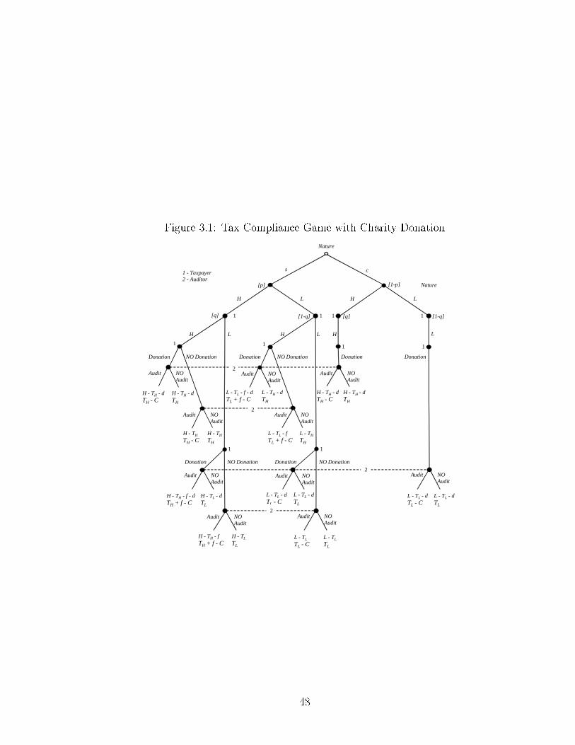
Figure 3.1: Tax Compliance Game with Charity Donation

L - TL - dTL

L - TL - dTL - C

L - TH

TH

L - TL - f TL + f - C

H - TH

TH

H - TH

TH - C

H - TH - dTH

L - TH - dTH

s c

Nature

[p] [1-p]

HH L L

[q] [1-q] [1-q][q]

HH L L H L

Donation NO Donation Donation NO Donation

Donation NO Donation Donation NO Donation

Donation Donation

Audit NOAudit

Audit NOAudit

Audit NOAudit

Audit NOAudit

Audit NOAudit

Audit NOAudit

Audit NOAudit

Audit NOAudit

Audit NOAudit

Audit NOAudit

H - TH - dTH - C

H - TH - dTH

L - TL - f - dTL + f - C

H - TH - f - dTH + f - C

H - TL - dTL

H - TH - f TH + f - C

H - TL

TL

L - TL

TL - CL - TL

TL

H - TH - dTH - C

L - TL - dTL - C

L - TL - dTL

Nature

2

2

2

2

1 - Taxpayer2 - Auditor

1 1 1 1

1111

11

48

In the Graetz et al. model that had compliant types, there was no way for a tax-

payer to convey any information to the auditor regarding his type in this dimension.

In our framework, we introduce a charitable donation D ∈ {0, d}, d > 0 that can

serve as a costly signal, that is correlated with the compliant type. Otherwise, the

donation has no impact on the tax liability of the taxpayer.

Assumption 2. Compliant types always donate to charity, D(x, c) = d, irre-

spective of income.

This assumption is strong, but can be relaxed without changing the qualitative

nature of the results. Since compliant types do not respond to model parameters, we

could assume some fraction of these players donate to charity, which will a�ect the

equilibrium probability of donation for the strategic players.

The proportion of the population reporting low income and giving to charity is

(1− p)(1− q).

This follows from Assumptions 1 and 2.

If the taxpayer is discovered to be misreporting his income by an auditor, he must

pay a �ne, F ∈ {0, f}, that will be positive f > 0 if he has misreported his income,

x 6= R, and 0 otherwise. There is no cost to that taxpayer if he is audited and

truthfully reporting his income.

All strategic taxpayers are risk neutral and have an expected utility, EU(R, D|x, s) =

x−D− [1−Prob(audit)]T (R)−Prob(audit)(T (x)+F (x, R)) that depends on signal

pair (R, D).

Also, min{H − TH , L − TL} > d, the all players would have net income greater

than zero after paying taxes and making the charitable donation and the penalty for

under-reporting is greater than the donation, f > d, so that we are not forced to

trivially eliminate the donation option for high income strategic individuals.

49

Low income strategic types will never report high income. That is, R(L, s) = L .

For any probability of audit, b, that the low income strategic taxpayer with ex-

pected utility, EU(R, D|L, s) = L − D − (1 − b)T (R) + −b(TL + F (x, R)) chooses

a signal pair (R, D). If the taxpayer reports high income, then his utility will be

EU(R, D|L, s) = L − D − (1 − b)TH − b(TL − f) which is strictly less than his

expected utility if he reports truthfully, EU(R, D|L, s) = L−TL−D since TH ≥ TL.

Strategic types who report truthfully will never make a donation. That is, if

R(x, s) = x then D(x, s) = 0.

Since an audit has no e�ect on the payo� of any honest report, it follows that for

any D > 0, the taxpayer's utility lower, therefore D = 0; rational optimizers have no

direct incentive to make a donation to charity.

Since low income strategic types will always play a pure strategy of low income and

no donation, (L, 0), only the high income strategic type may play a mixed strategy

where he chooses between the three possible signal pairs: (L, 0), (L, d) and (H, 0).

A mixed strategy for a high income strategic type is a probability distribution over

the possible signal pairs. The probability the taxpayer under-reports without making

a donation to charity, (L, 0), is α0 ≥ 0, the probability the taxpayer under-reports

and makes a donation to charity, (L, d) , is α1 ≥ 0 and the probability of submitting

a truthful report, (H, 0), to the auditor is (1− α0 − α1).

The taxpayer's signal pair, (R, D) is viewed by an auditor who must decide

whether to engage in an audit, A ∈ {0, 1}, that costs C to undertake.

The tax authority and auditor's objective is to maximize revenue net of audit

costs.

High reports are never audited as long as TH > TL + f − C.

50

The audit revenue depends on the auditor's decision to audit and whether the

report from the taxpayer was truthful: Π (A|R) = T (R)+A(T (x)−T (R)+F (x,R)−

C). If A = 1, then if the report was truthful, R = H, results in net revenue Π (A|H) =

TH − C < TH , that is lower than in the no audit case. If the report was not truthful

and an audit was initiated then the net revenue Π (A|H) = TL + F − C < TH . The

focus of the auditor's e�orts will be on identifying those taxpayers with a low report

who actually received a high income.

The auditor's beliefs, µ, regarding the taxpayer type given the signal pairs of low

income reports without and with a donation are the following:

µ (αi|D) =

qα0

qα0 + 1− qpqα1

pqα1 + (1− p)(1− q)

i = 0, if D = 0

i = 1, if D = d

A low income report without a donation will either come from a strategic player

with high income who under-reports with probability pqα0 or a strategic low income

earner, p(1 − q). Because only strategic players refrain from donating, the audi-

tor's beliefs regarding the taxpayer type, (x, y), is independent of relative size of the

strategic population, p.

A mixed strategy for an auditor is a conditional probability distribution over the

possible signal pairs he could receive. The probability of audit given a low report

without a charity donation, (L, 0) is β0 and the probability of audit given a low

report with a charity donation, (L, d) is β1.

The auditor's maximization problem is conditional on the report of high or low

income and whether a donation was made. The trivial cases of a high income report

with and without donation will not induce an audit. The risk neutral auditor maxi-

51

mizes revenue net audit costs in the sequential game where the taxpayer is the �rst

mover and has made a low income report:

Maxβi

Π (α0, α1, βi|D) = βi [µi (TH + f − C) + (1− µi) (TL − C)] + (1− βi)TL,

where i = 0 if D = 0 and i = 1 if D = d.

The cuto� belief above which the auditor will always audit a report and below

which he will never audit is µi =C

TH + F − TL, i = 0, 1.

The �rst order condition will determine the auditor's cuto� belief regarding the

proportion of misreporting in the population. He will be indi�erent between auditing

and not at the point where the net expected marginal return to an audit equals

the marginal cost. The probability of audit will be 1 whenever the proportion of

misreported incomes is above the cuto� value and 0 if the proportion falls below:

βi =

1 if µ (αi) > µi

[0, 1] if µ (αi) = µi

0 if µ (αi) < µi

for i = 0, 1.

The cuto� value of misreported income, µ, depends on the cost, tax and penalty

parameters, so is not restricted to take on a value less than 1. Clearly, if µ > 1, the

auditor will never audit.

The equilibrium strategy for strategic high income earner is characterized by the

following probabilities:

α∗i =

αi if 1 ≥ α0 + α1 ≥ 0αi

α0 + α1

if α0 + α1 > 1for i = 0, 1.

The cuto� µi determines αi, i = 0, 1, from the auditor's beliefs regarding the

proportion of low income reports that are untrue:

52

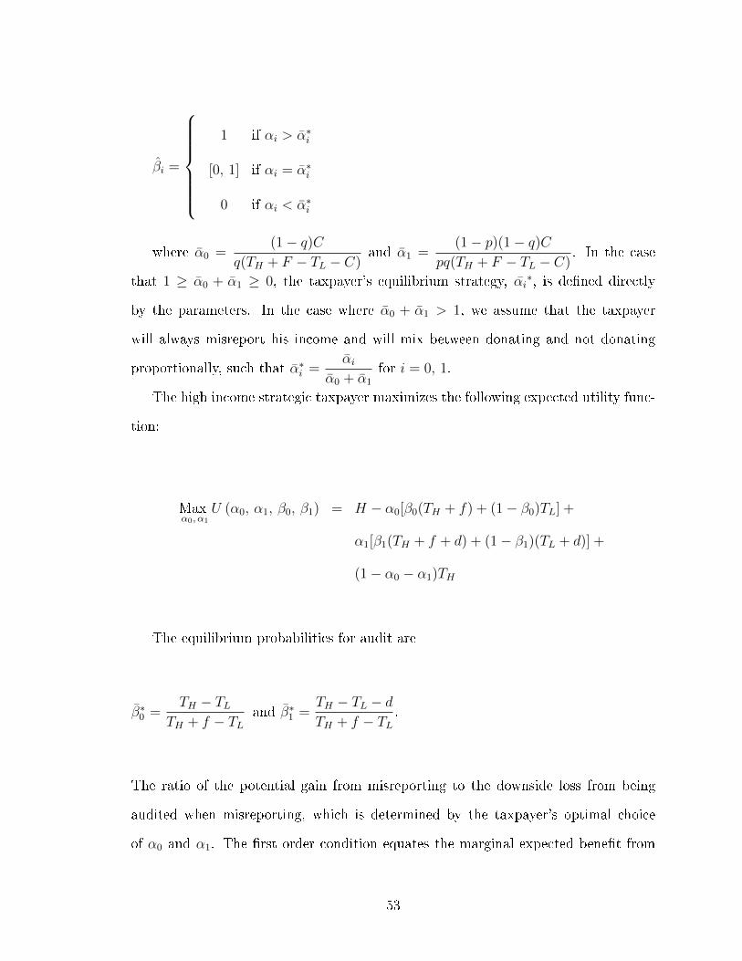
βi =

1 if αi > α∗

i

[0, 1] if αi = α∗i

0 if αi < α∗i

where α0 =(1− q)C

q(TH + F − TL − C)and α1 =

(1− p)(1− q)Cpq(TH + F − TL − C)

. In the case

that 1 ≥ α0 + α1 ≥ 0, the taxpayer's equilibrium strategy, αi∗, is de�ned directly

by the parameters. In the case where α0 + α1 > 1, we assume that the taxpayer

will always misreport his income and will mix between donating and not donating

proportionally, such that α∗i =

αiα0 + α1

for i = 0, 1.

The high income strategic taxpayer maximizes the following expected utility func-

tion:

Maxα0, α1

U (α0, α1, β0, β1) = H − α0[β0(TH + f) + (1− β0)TL] +

α1[β1(TH + f + d) + (1− β1)(TL + d)] +

(1− α0 − α1)TH

The equilibrium probabilities for audit are

β∗0 =

TH − TLTH + f − TL

and β∗1 =

TH − TL − dTH + f − TL

.

The ratio of the potential gain from misreporting to the downside loss from being

audited when misreporting, which is determined by the taxpayer's optimal choice

of α0 and α1. The �rst order condition equates the marginal expected bene�t from

53

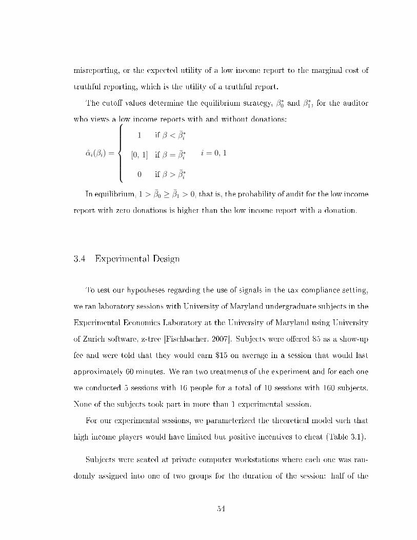
misreporting, or the expected utility of a low income report to the marginal cost of

truthful reporting, which is the utility of a truthful report.

The cuto� values determine the equilibrium strategy, β∗0 and β∗

1 , for the auditor

who views a low income reports with and without donations:

αi(βi) =

1 if β < β∗

i

[0, 1] if β = β∗i

0 if β > β∗i

i = 0, 1

In equilibrium, 1 > β0 ≥ β1 > 0, that is, the probability of audit for the low income

report with zero donations is higher than the low income report with a donation.

3.4 Experimental Design

To test our hypotheses regarding the use of signals in the tax compliance setting,

we ran laboratory sessions with University of Maryland undergraduate subjects in the

Experimental Economics Laboratory at the University of Maryland using University

of Zurich software, z-tree [Fischbacher, 2007]. Subjects were o�ered $5 as a show-up

fee and were told that they would earn $15 on average in a session that would last

approximately 60 minutes. We ran two treatments of the experiment and for each one

we conducted 5 sessions with 16 people for a total of 10 sessions with 160 subjects.

None of the subjects took part in more than 1 experimental session.

For our experimental sessions, we parameterized the theoretical model such that

high income players would have limited but positive incentives to cheat (Table 3.1).

Subjects were seated at private computer workstations where each one was ran-

domly assigned into one of two groups for the duration of the session: half of the

54

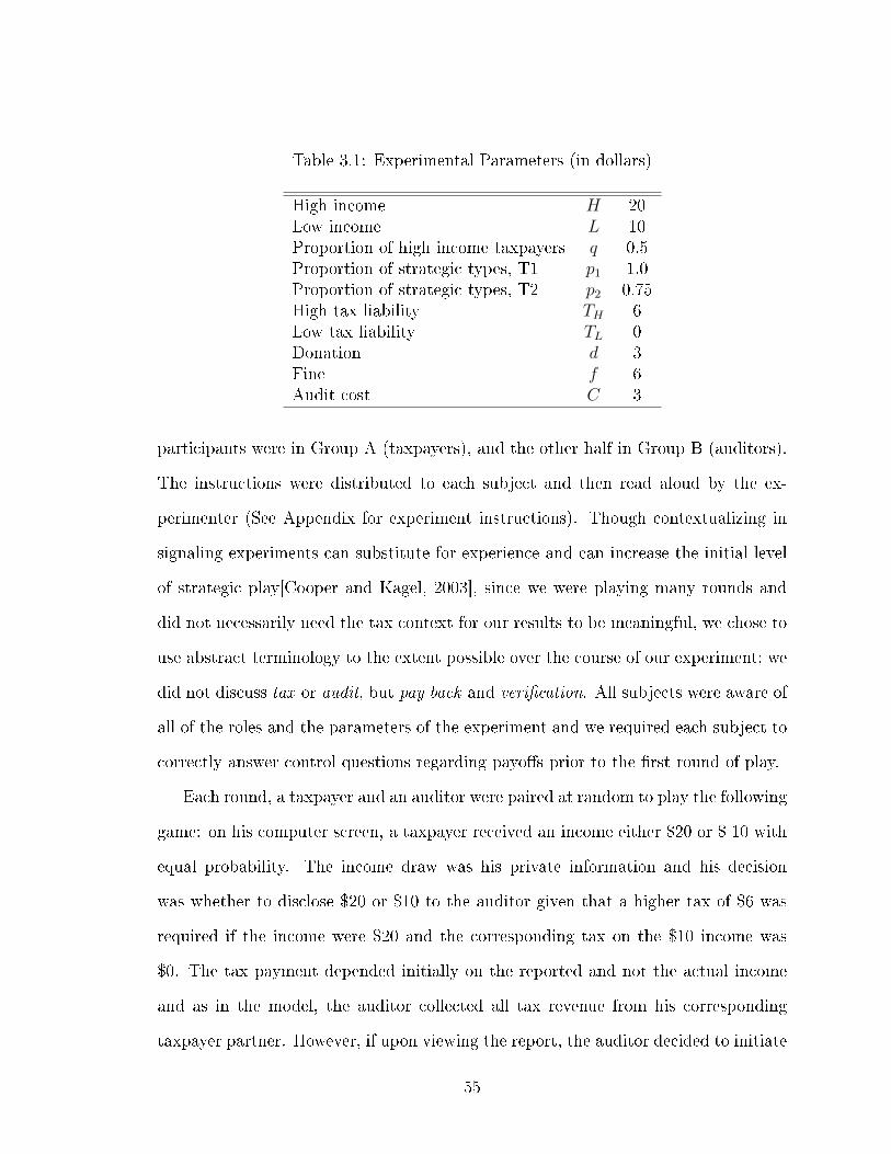
Table 3.1: Experimental Parameters (in dollars)

High income H 20Low income L 10Proportion of high income taxpayers q 0.5Proportion of strategic types, T1 p1 1.0Proportion of strategic types, T2 p2 0.75High tax liability TH 6Low tax liability TL 0Donation d 3Fine f 6Audit cost C 3

participants were in Group A (taxpayers), and the other half in Group B (auditors).

The instructions were distributed to each subject and then read aloud by the ex-

perimenter (See Appendix for experiment instructions). Though contextualizing in

signaling experiments can substitute for experience and can increase the initial level

of strategic play[Cooper and Kagel, 2003], since we were playing many rounds and

did not necessarily need the tax context for our results to be meaningful, we chose to

use abstract terminology to the extent possible over the course of our experiment; we

did not discuss tax or audit, but pay back and veri�cation. All subjects were aware of

all of the roles and the parameters of the experiment and we required each subject to

correctly answer control questions regarding payo�s prior to the �rst round of play.

Each round, a taxpayer and an auditor were paired at random to play the following

game: on his computer screen, a taxpayer received an income either $20 or $ 10 with

equal probability. The income draw was his private information and his decision

was whether to disclose $20 or $10 to the auditor given that a higher tax of $6 was

required if the income were $20 and the corresponding tax on the $10 income was

$0. The tax payment depended initially on the reported and not the actual income

and as in the model, the auditor collected all tax revenue from his corresponding

taxpayer partner. However, if upon viewing the report, the auditor decided to initiate

55

Table 3.2: Taxpayer Payo�s

High IncomeNo Donation Audit Donation Audit

No Yes No YesReport High 14 14 Report High 11 11

Low 20 8 Low 17 5

Low IncomeNo Donation Audit Donation Audit

No Yes No YesReport High 4 4 Report High 1 1

Low 10 10 Low 7 7

an audit, he learned the actual income of the taxpayer and if it di�ered from the

reported amount, that taxpayer was required to pay a $6 �ne in addition to the

unpaid tax liability (which could be negative in the case of over-reporting of income).

The taxpayer was also given the option to make an observable and veri�able donation

to a University of Maryland charity,2 where the donation was immediately subtracted

from the income and had no impact on the tax liability of the taxpayer. We chose

this simpli�cation rather than one that is closer to reality where charity donations

are essentially subsidized in the tax code, because donations still represent a loss to

the individual, with or without any added incentives.

The taxpayer's payo�s in all possible scenarios, Table 3.2, were given to all players

to ensure that the stakes of the game were clearly understood.

After viewing his partner's reported income and charity donation, the auditor was

given the option to verify the income report. An auditor incurred a cost of $3 if he

decided to verify his partner's income, but we provided each auditor with the $3 audit

cost in order to avoid any complications, both in terms of logistics and behavior, if

in fact we made participants take losses in the experiment. If the auditor chose not

2The charity selected was the University of Maryland's Maryland Fund for Excellence, the Uni-versity's umbrella fundraising vehicle.

56

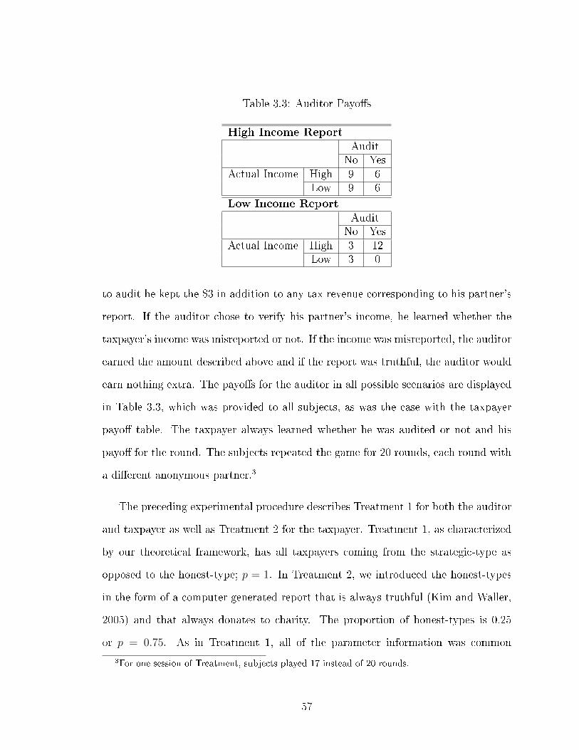
Table 3.3: Auditor Payo�s

High Income ReportAudit

No YesActual Income High 9 6

Low 9 6

Low Income ReportAudit

No YesActual Income High 3 12

Low 3 0

to audit he kept the $3 in addition to any tax revenue corresponding to his partner's

report. If the auditor chose to verify his partner's income, he learned whether the

taxpayer's income was misreported or not. If the income was misreported, the auditor

earned the amount described above and if the report was truthful, the auditor would

earn nothing extra. The payo�s for the auditor in all possible scenarios are displayed

in Table 3.3, which was provided to all subjects, as was the case with the taxpayer

payo� table. The taxpayer always learned whether he was audited or not and his

payo� for the round. The subjects repeated the game for 20 rounds, each round with

a di�erent anonymous partner.3

The preceding experimental procedure describes Treatment 1 for both the auditor

and taxpayer as well as Treatment 2 for the taxpayer. Treatment 1, as characterized

by our theoretical framework, has all taxpayers coming from the strategic-type as

opposed to the honest-type; p = 1. In Treatment 2, we introduced the honest-types

in the form of a computer generated report that is always truthful (Kim and Waller,

2005) and that always donates to charity. The proportion of honest-types is 0.25

or p = 0.75. As in Treatment 1, all of the parameter information was common

3For one session of Treatment, subjects played 17 instead of 20 rounds.

57

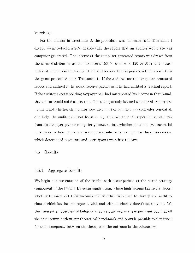
knowledge.

For the auditor in Treatment 2, the procedure was the same as in Treatment 1

except we introduced a 25% chance that the report that an auditor would see was

computer generated. The income of the computer generated report was drawn from

the same distribution as the taxpayer's (50/50 chance of $20 or $10) and always

included a donation to charity. If the auditor saw the taxpayer's actual report, then

the game proceeded as in Treatment 1. If the auditor saw the computer generated

report and audited it, he would receive payo�s as if he had audited a truthful report.

If the auditor's corresponding taxpayer pair had misreported his income in that round,

the auditor would not discover this. The taxpayer only learned whether his report was

audited, not whether the auditor view his report or one that was computer generated.

Similarly, the auditor did not learn at any time whether the report he viewed was

from his taxpayer pair or computer generated, just whether his audit was successful

if he chose to do so. Finally, one round was selected at random for the entire session,

which determined payments and participants were free to leave.

3.5 Results

3.5.1 Aggregate Results

We begin our presentation of the results with a comparison of the mixed strategy

component of the Perfect Bayesian equilibrium, where high income taxpayers choose

whether to misreport their incomes and whether to donate to charity and auditors

choose which low income reports, with and without charity donations, to audit. We

then present an overview of behavior that we observed in the experiment but that o�

the equilibrium path in our theoretical benchmark and provide possible explanations

for the discrepancy between the theory and the outcome in the laboratory.

58

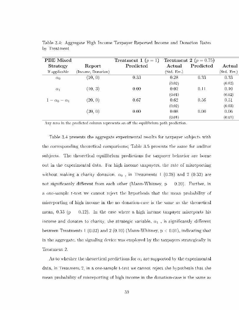
Table 3.4: Aggregate High Income Taxpayer Reported Income and Donation Ratesby Treatment

PBE Mixed Treatment 1 (p = 1) Treatment 2 (p = 0.75)Strategy Report Predicted Actual Predicted ActualIf applicable (Income, Donation) (Std. Err.) (Std. Err.)

α0 (10, 0) 0.33 0.28 0.33 0.33(0.02) (0.02)

α1 (10, 3) 0.00 0.02 0.11 0.10(0.01) (0.02)

1− α0 − α1 (20, 0) 0.67 0.62 0.56 0.51(0.02) (0.03)

(20, 0) 0.00 0.08 0.00 0.06(0.01) (0.01)

Any zero in the predicted column represents an o� the equilibrium path prediction.

Table 3.4 presents the aggregate experimental results for taxpayer subjects with

the corresponding theoretical comparisons; Table 3.5 presents the same for auditor

subjects. The theoretical equilibrium predictions for taxpayer behavior are borne

out in the experimental data. For high income taxpayers, the rate of misreporting

without making a charity donation, α0 , in Treatments 1 (0.28) and 2 (0.33) are

not signi�cantly di�erent from each other (Mann-Whitney, p = 0.20). Further, in

a one-sample t-test we cannot reject the hypothesis that the mean probability of

misreporting of high income in the no donation-case is the same as the theoretical

mean, 0.33 (p = 0.12). In the case where a high income taxpayer misreports his

income and donates to charity, the strategic variable, α1 , is signi�cantly di�erent

between Treatments 1 (0.02) and 2 (0.10) (Mann-Whitney, p < 0.01), indicating that

in the aggregate, the signaling device was employed by the taxpayers strategically in

Treatment 2.

As to whether the theoretical predictions for α1 are supported by the experimental

data, in Treatment 2, in a one-sample t-test we cannot reject the hypothesis that the

mean probability of misreporting of high income in the donation-case is the same as

59

Table 3.5: Aggregate Audit Rates Conditional on Viewed Income Report and Dona-tion by Treatment

PBE Mixed Treatment 1 (p = 1) Treatment 2 (p = 0.75)Strategy Viewed Report Predicted Actual Predicted ActualIf applicable (Income, Donation) (Std. Err.) (Std. Err.)

β0 (10, 0) 0.50 0.53 0.50 0.56(0.02) (0.03)

β1 (10, 3) 0 0.65 0.25 0.45(0.11) (0.04)

(20, 0) 0 0.25 0 0.17(0.03) (0.03)

(20,3) 0 0.36 0 0.14(0.08) (0.03)

Any zero in the predicted column represents an o� the equilibrium path prediction.

the theoretical mean, 0.11 (p = 0.54). However for α1, Treatment 1, in a one-sample

t-test we reject the hypothesis that the mean probability of misreporting of high

income in the donation-case is the same as the theoretical mean of zero (p = 0.01).

A possible accounting for this behavior could be social preferences.

We considered individuals who displayed a social preference to be those who do-

nated to charity even when they received a low income. In Treatment 1, 4.0% of

low income draws were accompanied by a donation and in Treatment 2, 4.5%. These

values were not signi�cantly di�erent across treatments (Mann-Whitney, p = 0.719).

When we exclude any individual who has displayed a social preference, the result is

the same value for α1 of 0.02 which is signi�cantly di�erent from zero (p = 0.01).

When we exclude Rounds 6-20 from our calculation of α0 we arrive at the theoretical

result for Treatment 1, α1 = 0, (t-test p = 0.158), indicating that though subjects

may had an initial inclination to donate to charity, as the game progressed, they were

converging to the equilibrium. Subsequent regression results will con�rm this (Table

3.9).

60

Aggregate auditor behavior (Table 3.5) is less in line with the theory, particularly

for the audit rates of a low income report with a donation. But we do �nd, in contrast

with the experimental results of Kim and Waller 2005, the theoretical insensitivity

of β0 to p holds when we introduce the charity signal. Mann-Whitney test indicates

that the experimental β0's in Treatments 1 (0.53) and 2 (0.56) are not signi�cantly

di�erent from each other (p = 0.36). Further, in a one-sample t-test, we can reject

the hypothesis that the mean probability of misreporting of high income in the no

donation-case is the same as the theoretical mean, 0.5 (p < 0.01); auditors are auditing

more frequently than the theory predicts. Mann-Whitney test indicates that the

experimental β1 in Treatments 1 (0.65, 20 observations) and 2 (0.45, 133 observations)

are signi�cantly di�erent from each other at the 10 percent level (p = 0.10).

For both taxpayer and auditor participants, we observed o� the equilibrium path

behavior in our model, such as donations when incomes were low, over-reporting of

income and auditing of high income reports. We can attribute it to subject confusion

only to a certain extent: the control questions administered at the beginning of the

experiment were meant to improve subject understanding of the payo�s. As shown

in Table 3.5, auditors were verifying high income reports at rates much higher than

zero: 25 percent (without donation) to 36 percent (with donation) in Treatment 1

and 17 percent (without donation) and 14 percent (with donation) in Treatment 2.

Even given that taxpayers were over-reporting their incomes, the best response of the

auditor would still be to refrain from auditing as he would lose $3 and only receive $6

in the event that a low income taxpayer was over-reporting as opposed to receiving

$9 for certain.

Table 3.6 shows that aggregate taxpayer behavior given low income is as the theory

predicts. However 3 percent in Treatment 1 and 4 percent of subjects in Treatment 2

give to charity when they have a low income. Also, 4 percent of subjects over report

61

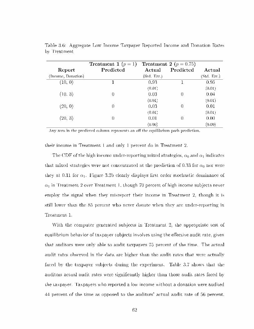
Table 3.6: Aggregate Low Income Taxpayer Reported Income and Donation Ratesby Treatment

Treatment 1 (p = 1) Treatment 2 (p = 0.75)Report Predicted Actual Predicted Actual

(Income, Donation) (Std. Err.) (Std. Err.)

(10, 0) 1 0.93 1 0.95(0.01) (0.01)

(10, 3) 0 0.03 0 0.04(0.01) (0.01)

(20, 0) 0 0.03 0 0.01(0.01) (0.01)

(20, 3) 0 0.01 0 0.00(0.00) (0.00)

Any zero in the predicted column represents an o� the equilibrium path prediction.

their income in Treatment 1 and only 1 percent do in Treatment 2.

The CDF of the high income under-reporting mixed strategies, α0 and α1 indicates

that mixed strategies were not concentrated at the prediction of 0.33 for α0 nor were

they at 0.11 for α1. Figure 3.2b clearly displays �rst order stochastic dominance of

α1 in Treatment 2 over Treatment 1, though 70 percent of high income subjects never

employ the signal when they misreport their income in Treatment 2, though it is

still lower than the 85 percent who never donate when they are under-reporting in

Treatment 1.

With the computer generated subjects in Treatment 2, the appropriate test of

equilibrium behavior of taxpayer subjects involves using the e�ective audit rate, given

that auditors were only able to audit taxpayers 75 percent of the time. The actual

audit rates observed in the data are higher than the audit rates that were actually

faced by the taxpayer subjects during the experiment. Table 3.7 shows that the

auditors actual audit rates were signi�cantly higher than those audit rates faced by

the taxpayer. Taxpayers who reported a low income without a donation were audited

44 percent of the time as opposed to the auditors' actual audit rate of 56 percent.

62

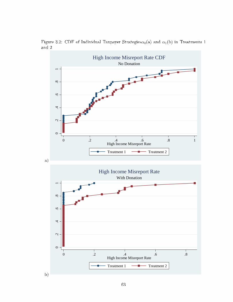
Figure 3.2: CDF of Individual Taxpayer Strategiesα0(a) and α1(b) in Treatments 1and 2

a)

0.2

.4.6

.81

0 .2 .4 .6 .8 1High Income Misreport Rate

Treatment 1 Treatment 2

No DonationHigh Income Misreport Rate CDF

b)

0.2

.4.6

.81

0 .2 .4 .6 .8High Income Misreport Rate

Treatment 1 Treatment 2

With DonationHigh Income Misreport Rate

63

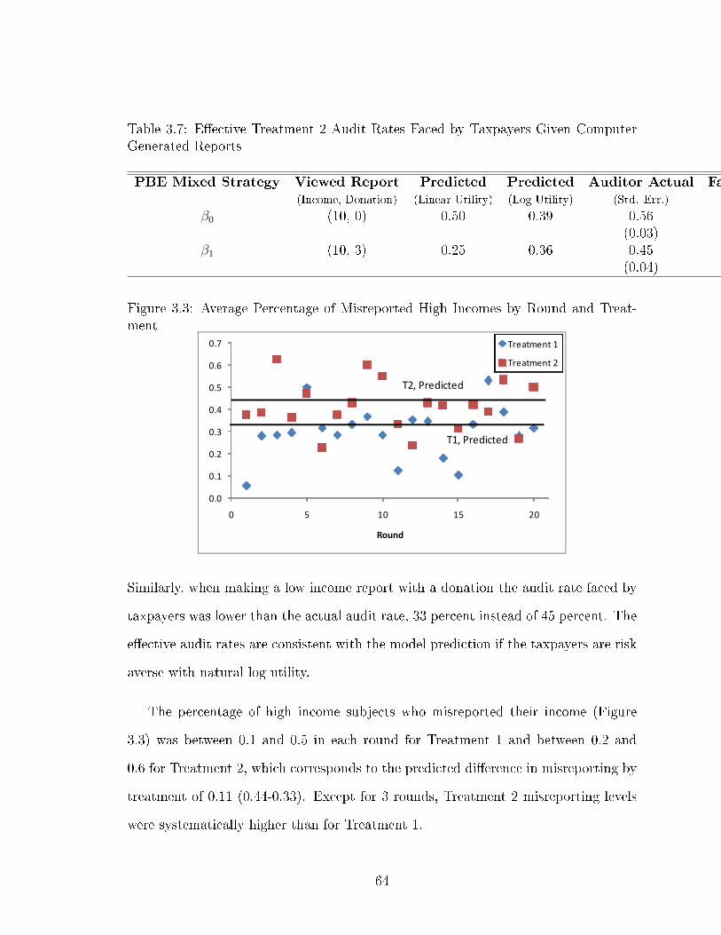
Table 3.7: E�ective Treatment 2 Audit Rates Faced by Taxpayers Given ComputerGenerated Reports

PBE Mixed Strategy Viewed Report Predicted Predicted Auditor Actual Faced by Taxpayer(Income, Donation) (Linear Utility) (Log Utility) (Std. Err.) (Std. Err.)

β0 (10, 0) 0.50 0.39 0.56 0.44(0.03) (0.02)

β1 (10, 3) 0.25 0.36 0.45 0.33(0.04) (0.06)

Figure 3.3: Average Percentage of Misreported High Incomes by Round and Treat-ment

���

���

���

���

���

���

���

��

� � �� �� ��

�����

�� �������

�� �������

��� �������

��� �������

Similarly, when making a low income report with a donation the audit rate faced by

taxpayers was lower than the actual audit rate, 33 percent instead of 45 percent. The

e�ective audit rates are consistent with the model prediction if the taxpayers are risk

averse with natural log utility.

The percentage of high income subjects who misreported their income (Figure

3.3) was between 0.1 and 0.5 in each round for Treatment 1 and between 0.2 and

0.6 for Treatment 2, which corresponds to the predicted di�erence in misreporting by

treatment of 0.11 (0.44-0.33). Except for 3 rounds, Treatment 2 misreporting levels

were systematically higher than for Treatment 1.

64

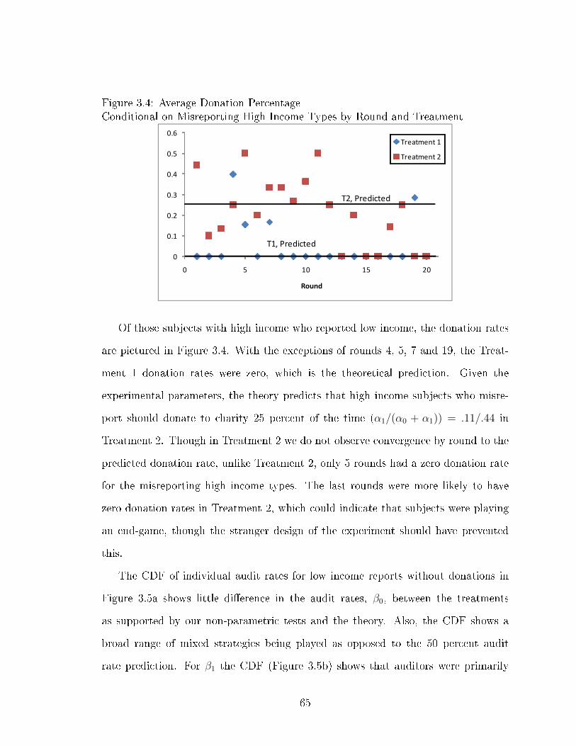
Figure 3.4: Average Donation PercentageConditional on Misreporting High Income Types by Round and Treatment

�

���

���

���

���

���

���

� � �� �� ��

�����

�� ��� ��

�� ��� ��

�����������

��� �������

Of those subjects with high income who reported low income, the donation rates

are pictured in Figure 3.4. With the exceptions of rounds 4, 5, 7 and 19, the Treat-

ment 1 donation rates were zero, which is the theoretical prediction. Given the

experimental parameters, the theory predicts that high income subjects who misre-

port should donate to charity 25 percent of the time (α1/(α0 + α1)) = .11/.44 in

Treatment 2. Though in Treatment 2 we do not observe convergence by round to the

predicted donation rate, unlike Treatment 2, only 5 rounds had a zero donation rate

for the misreporting high income types. The last rounds were more likely to have

zero donation rates in Treatment 2, which could indicate that subjects were playing

an end-game, though the stranger design of the experiment should have prevented

this.

The CDF of individual audit rates for low income reports without donations in

Figure 3.5a shows little di�erence in the audit rates, β0, between the treatments

as supported by our non-parametric tests and the theory. Also, the CDF shows a

broad range of mixed strategies being played as opposed to the 50 percent audit

rate prediction. For β1 the CDF (Figure 3.5b) shows that auditors were primarily

65

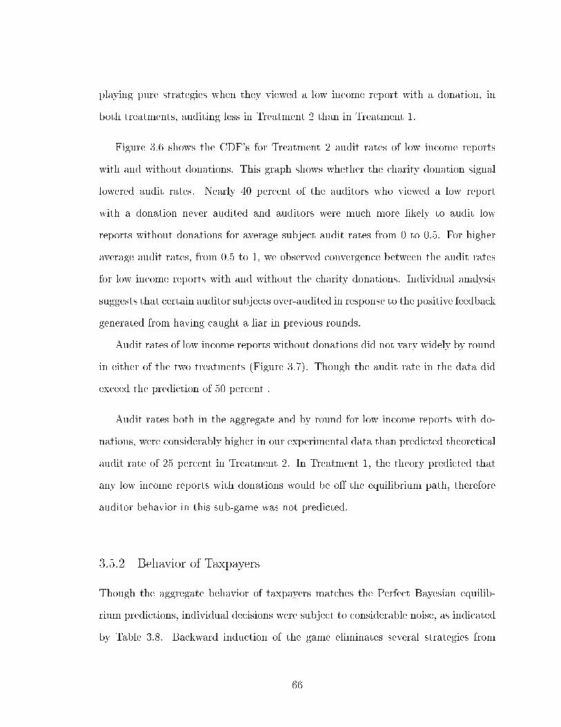
playing pure strategies when they viewed a low income report with a donation, in

both treatments, auditing less in Treatment 2 than in Treatment 1.

Figure 3.6 shows the CDF's for Treatment 2 audit rates of low income reports

with and without donations. This graph shows whether the charity donation signal

lowered audit rates. Nearly 40 percent of the auditors who viewed a low report

with a donation never audited and auditors were much more likely to audit low

reports without donations for average subject audit rates from 0 to 0.5. For higher

average audit rates, from 0.5 to 1, we observed convergence between the audit rates

for low income reports with and without the charity donations. Individual analysis

suggests that certain auditor subjects over-audited in response to the positive feedback

generated from having caught a liar in previous rounds.

Audit rates of low income reports without donations did not vary widely by round

in either of the two treatments (Figure 3.7). Though the audit rate in the data did

exceed the prediction of 50 percent .

Audit rates both in the aggregate and by round for low income reports with do-

nations, were considerably higher in our experimental data than predicted theoretical

audit rate of 25 percent in Treatment 2. In Treatment 1, the theory predicted that

any low income reports with donations would be o� the equilibrium path, therefore

auditor behavior in this sub-game was not predicted.

3.5.2 Behavior of Taxpayers

Though the aggregate behavior of taxpayers matches the Perfect Bayesian equilib-

rium predictions, individual decisions were subject to considerable noise, as indicated

by Table 3.8. Backward induction of the game eliminates several strategies from

66

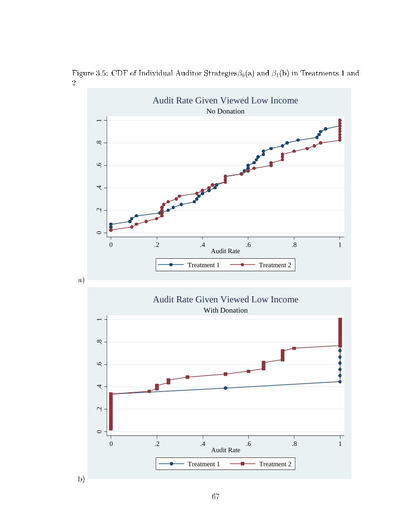
Figure 3.5: CDF of Individual Auditor Strategiesβ0(a) and β1(b) in Treatments 1 and2

a)

0.2

.4.6

.81

0 .2 .4 .6 .8 1Audit Rate

Treatment 1 Treatment 2

No DonationAudit Rate Given Viewed Low Income

b)

0.2

.4.6

.81

0 .2 .4 .6 .8 1Audit Rate

Treatment 1 Treatment 2

With DonationAudit Rate Given Viewed Low Income

67

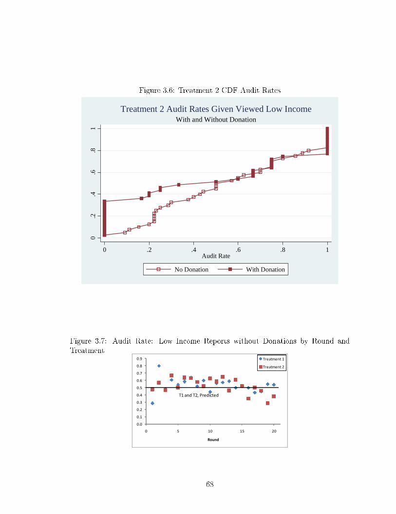
Figure 3.6: Treatment 2 CDF Audit Rates0

.2.4

.6.8

1

0 .2 .4 .6 .8 1Audit Rate

No Donation With Donation

With and Without DonationTreatment 2 Audit Rates Given Viewed Low Income

Figure 3.7: Audit Rate: Low Income Reports without Donations by Round andTreatment

���

���

���

���

���

���

���

��

��

���

� � �� �� ��

�����

� ���������

� ���������

���������� ��� ���

68

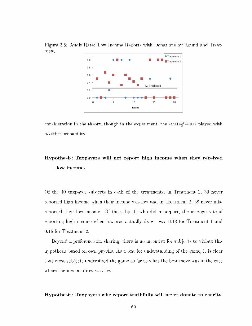
Figure 3.8: Audit Rate: Low Income Reports with Donations by Round and Treat-ment

���

���

���

���

���

���

� � �� �� ��

�����

�� ��� ��

�� ��� ��

��� �������

consideration in the theory, though in the experiment, the strategies are played with

positive probability.

Hypothesis: Taxpayers will not report high income when they received

low income.

Of the 40 taxpayer subjects in each of the treatments, in Treatment 1, 30 never

reported high income when their income was low and in Treatment 2, 38 never mis-

reported their low income. Of the subjects who did misreport, the average rate of

reporting high income when low was actually drawn was 0.18 for Treatment 1 and

0.16 for Treatment 2.

Beyond a preference for sharing, there is no incentive for subjects to violate this

hypothesis based on own payo�s. As a test for understanding of the game, it is clear

that most subjects understood the game as far as what the best move was in the case

where the income draw was low.

Hypothesis: Taxpayers who report truthfully will never donate to charity.

69

Of the low income earners who always reported low income 7 in Treatment 1 and 9

in Treatment 2 donated to charity. As for the truthful reports of high income, 26

subjects in Treatment 1 and 30 subjects in Treatment 2 never made donations. Of

those subjects who reported low income when their income was low and never gave

to charity when truthfully reporting, 4 in Treatment 1 and 7 in Treatment 2 used the

charity donation as a signal.

Hypothesis: Taxpayers will misreport their income when it is high while

donating to charity only when some of the players are honest-types,

p < 1.

Signaling behavior was observed in both treatments, in a manner that is in line with

the predictions, namely that more signaling behavior will be observed in Treatment 2

than in Treatment 1. In Treatment 1, 6 subjects used the signal and in Treatment 2,

13 did. When we identify which of those subjects do not display any preferences for

make a donation when their income is high, the number of subjects using the signal

drops in each treatment, to 5 in Treatment 1 and 8 in Treatment 2.

As for those subjects who made consistent reports, in Treatment 1, 9 always

reported truthfully when earning high income and in Treatment 2, 5 subjects never

lied on high income draws. On the other side of the spectrum, only 1 subject in

Treatment 1 always reported low income when earning high income and 2 subjects

in Treatment 2. Finally, very few subjects donated when truthfully reporting high

income and did not donate when lying about their high income; 5 in Treatment 1 and

2 in Treatment 2.

70

Figure 3.9: Individual Taxpayer Behavior, Treatment 1 (A), Treatment 2 (B)

��

��

� � � � � �� �� �� �� �� ��

���� � ������ ���� ������ ������� �����

��

��

� � � � � �� �� �� �� �� ��

��

��

� � � � � �� �� �� �� �� ��

��

��

� � � � � �� �� �� �� �� ��

��

��

� � � � � �� �� �� �� �� ��

��

��

� � � � � �� �� �� �� �� ��

��

��

� � � � � �� �� �� �� �� ��

���� � ������ ���� ������ ������� ������

��

��

� � � � � �� �� �� �� �� ��

��

��

� � � � � �� �� �� �� �� ��

��

��

� � � � � �� �� �� �� �� ��

��

��

� � � � � �� �� �� �� �� ��

��

��

� � � � � �� �� �� �� �� ��

��

��

� � � � � �� �� �� �� �� ����

��

� � � � � �� �� �� �� �� ��

�

71

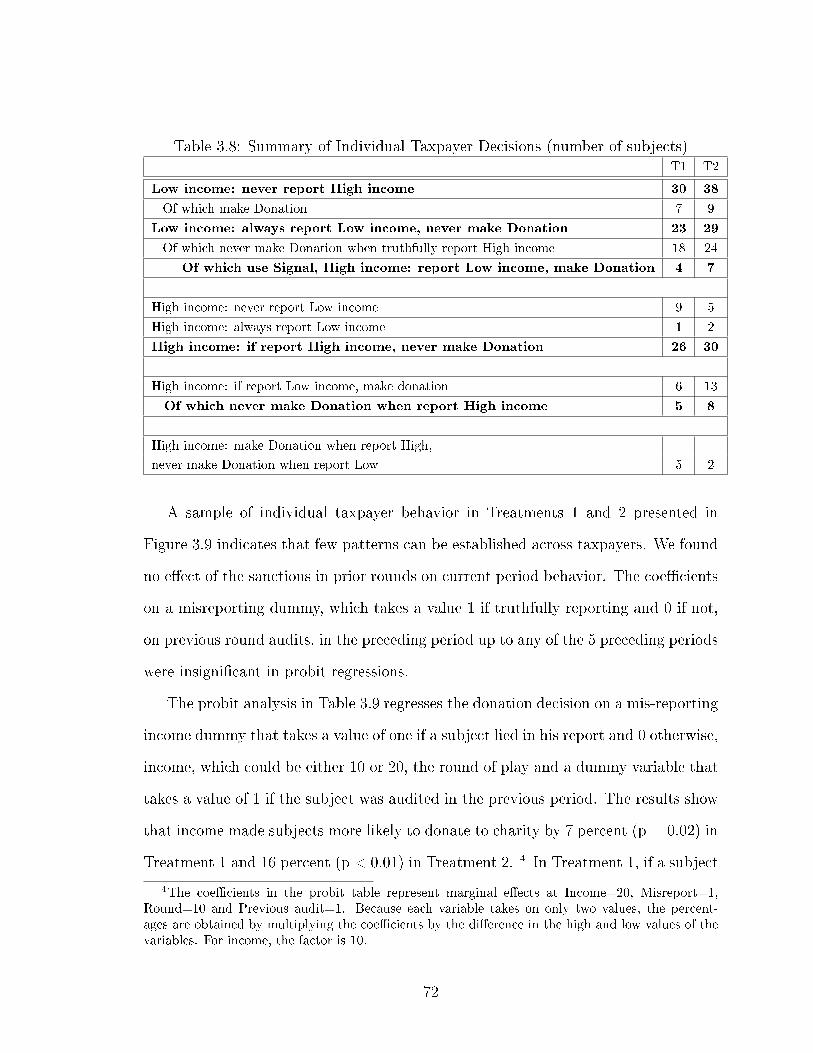
Table 3.8: Summary of Individual Taxpayer Decisions (number of subjects)T1 T2

Low income: never report High income 30 38

Of which make Donation 7 9

Low income: always report Low income, never make Donation 23 29

Of which never make Donation when truthfully report High income 18 24

Of which use Signal, High income: report Low income, make Donation 4 7

High income: never report Low income 9 5

High income: always report Low income 1 2

High income: if report High income, never make Donation 26 30

High income: if report Low income, make donation 6 13

Of which never make Donation when report High income 5 8

High income: make Donation when report High,

never make Donation when report Low 5 2

A sample of individual taxpayer behavior in Treatments 1 and 2 presented in

Figure 3.9 indicates that few patterns can be established across taxpayers. We found

no e�ect of the sanctions in prior rounds on current period behavior. The coe�cients

on a misreporting dummy, which takes a value 1 if truthfully reporting and 0 if not,

on previous round audits, in the preceding period up to any of the 5 preceding periods

were insigni�cant in probit regressions.

The probit analysis in Table 3.9 regresses the donation decision on a mis-reporting

income dummy that takes a value of one if a subject lied in his report and 0 otherwise,

income, which could be either 10 or 20, the round of play and a dummy variable that

takes a value of 1 if the subject was audited in the previous period. The results show

that income made subjects more likely to donate to charity by 7 percent (p = 0.02) in

Treatment 1 and 16 percent (p < 0.01) in Treatment 2. 4 In Treatment 1, if a subject

4The coe�cients in the probit table represent marginal e�ects at Income=20, Misreport=1,Round=10 and Previous audit=1. Because each variable takes on only two values, the percent-ages are obtained by multiplying the coe�cients by the di�erence in the high and low values of thevariables. For income, the factor is 10.

72

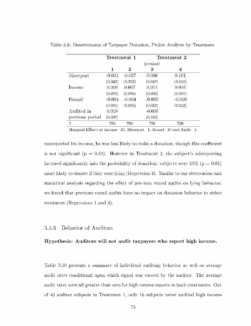
Table 3.9: Determinants of Taxpayer Donation, Probit Analysis by Treatment

Treatment 1 Treatment 2(p-value)

1 2 3 4Misreport -0.031 -0.027 0.086 0.101

(0.343) (0.352) (0.018) (0.010)

Income 0.008 0.007 0.014 0.016(0.018) (0.016) (0.002) (0.001)

Round -0.004 -0.004 -0.009 -0.010(0.081) (0.078) (0.013) (0.012)

Audited in 0.018 -0.056previous period (0.397) (0.169)

N 760 760 736 736

Marginal E�ects at Income=20, Misreport=1, Round=10 and Audit=1.

misreported his income, he was less likely to make a donation, though this coe�cient

is not signi�cant (p = 0.34). However in Treatment 2, the subject's misreporting

factored signi�cantly into the probability of donation: subjects were 10% (p = 0.01)

more likely to donate if they were lying (Regression 4). Similar to our observation and

statistical analysis regarding the e�ect of previous round audits on lying behavior,

we found that previous round audits have no impact on donation behavior in either

treatment (Regressions 1 and 3).

3.5.3 Behavior of Auditors

Hypothesis: Auditors will not audit taxpayers who report high income.

Table 3.10 presents a summary of individual auditing behavior as well as average

audit rates conditional upon which signal was viewed by the auditor. The average

audit rates were all greater than zero for high income reports in both treatments. Out

of 40 auditor subjects in Treatment 1, only 16 subjects never audited high income

73

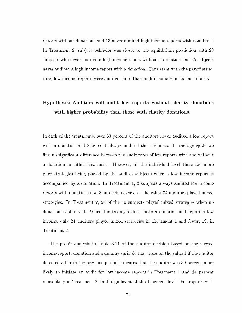
reports without donations and 13 never audited high income reports with donations.

In Treatment 2, subject behavior was closer to the equilibrium prediction with 29

subjects who never audited a high income report without a donation and 25 subjects

never audited a high income report with a donation. Consistent with the payo� struc-

ture, low income reports were audited more than high income reports and reports.

Hypothesis: Auditors will audit low reports without charity donations

with higher probability than those with charity donations.

In each of the treatments, over 50 percent of the auditors never audited a low report

with a donation and 8 percent always audited those reports. In the aggregate we

�nd no signi�cant di�erence between the audit rates of low reports with and without

a donation in either treatment. However, at the individual level there are more

pure strategies being played by the auditor subjects when a low income report is

accompanied by a donation. In Treatment 1, 3 subjects always audited low income

reports with donations and 3 subjects never do. The other 34 auditors played mixed

strategies. In Treatment 2, 28 of the 40 subjects played mixed strategies when no

donation is observed. When the taxpayer does make a donation and report a low

income, only 24 auditors played mixed strategies in Treatment 1 and fewer, 19, in

Treatment 2.

The probit analysis in Table 3.11 of the auditor decision based on the viewed

income report, donation and a dummy variable that takes on the value 1 if the auditor

detected a liar in the previous period indicates that the auditor was 39 percent more

likely to initiate an audit for low income reports in Treatment 1 and 24 percent

more likely in Treatment 2, both signi�cant at the 1 percent level. For reports with

74

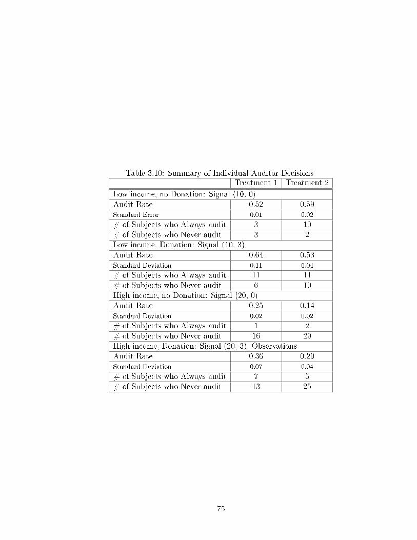
Table 3.10: Summary of Individual Auditor DecisionsTreatment 1 Treatment 2

Low income, no Donation: Signal (10, 0)Audit Rate 0.52 0.59Standard Error 0.01 0.02

# of Subjects who Always audit 3 10# of Subjects who Never audit 3 2Low income, Donation: Signal (10, 3)Audit Rate 0.64 0.53Standard Deviation 0.11 0.04

# of Subjects who Always audit 11 11# of Subjects who Never audit 6 10High income, no Donation: Signal (20, 0)Audit Rate 0.25 0.14Standard Deviation 0.02 0.02

# of Subjects who Always audit 1 2# of Subjects who Never audit 16 29High income, Donation: Signal (20, 3), ObservationsAudit Rate 0.36 0.20Standard Deviation 0.07 0.04

# of Subjects who Always audit 7 5# of Subjects who Never audit 13 25

75

Table 3.11: Probit: Independent Variable Audit (Marginal E�ects)

Treatment 1 Treatment 2(p-value)

Income Report -0.024 -0.039(0.000) (0.000)

Donation 0.037 -0.027(0.023) (0.060)

Caught a liar 0.086 0.176previous round (0.109) (0.006)

N 760 736

Marginal E�ects at Income=10, Donation=3 and Caught Liar=1.

a donation in Treatment 1, the coe�cient on donation of 0.037 represents an 11

percent increase in the probability of audit if a donation is viewed by the auditor.

5 The model predictions place zero probability on any donations being made if all

types are strategic. The positive and signi�cant coe�cient on donations in Treatment

1 one indicates that the charity donation may have been interpreted as a signal of

non-compliance without our prompting of the subjects in the opposite direction, as

we do in Treatment 2. As we see in Treatment 2, an auditor who viewed a charity

donation was 8 percent less likely to audit the report than if no donation had been

made. When we impose the computer generated subjects with 25 percent chance on

the auditor in Treatment 2, making it was less likely to catch a misreporting taxpayer

subject, the auditors response to catching a liar in the previous period becomes highly

signi�cant in determining whether he audits in the current period he was more likely

to audit: 9 percent more likely in Treatment 1 (p = 0.11) and 18 percent more likely

in Treatment 2 (p = 0.01). The signi�cant response to past experience in our result

suggests an adaptive learning process is in�uencing the auditor's equilibrium strategy.

5The coe�cients in the probit table represent marginal e�ects at Report=10 and Donation=3.Because each variable takes on only two values, the percentages are obtained by multiplying thecoe�cients by the di�erence in the high and low values of the variables. For income, the factor is10 and for the donation, the factor is 3.

76

3.6 Discussion and Conclusion

Though the aggregate likelihood of the use of a charity donation as signal of

honesty by taxpayers conforms with the numerical theoretical predictions, our results

indicate that at the individual level, the response to the change in composition of the

population when we introduced the compliant types was heterogeneous across subjects

and there was little indication that all subjects would converge to the equilibrium

strategy in additional rounds. In identify individual strategies across treatments and

in a binary choice model analysis of taxpayer behavior we found that on the margin,

there were more subjects who used the donation as a signal of honesty when the

proportion of compliant types in the population increased, p = 0.75. However, in the

treatment with compliant types the use of the signal by taxpayer subjects did not

increase for 27 out of 40 subjects when the theory would have predicted increased

probability of donation when under-reporting income for all subjects.

Auditor behavior in the experiment generally consistent with the Perfect Bayesian

equilibrium probabilities whether a low income report was or was not accompanied

by a donation; auditors audited low income reports without donations at higher rates

than they did low income reports with donations. However, we identi�ed subjects who

consistently over-audited low income reports (more than 50 percent of the time) which

drove aggregate audit rates higher than predicted. Also, audits were systematically

initiated o� the equilibrium path. We explain this by showing that auditors were

responding to feedback after having caught dishonest taxpayers in previous rounds.

Even with the higher audit rates played by auditor subjects in Treatment 2, taxpayers

faced audit rates that were in line with equilibrium predictions because of the lower

chance of audit with the computer generated reports. In this regard, the aggregate

taxpayer behavior is fully in line with the equilibrium predictions.

77

One aspect of the experimental assumption that all subjects will behave as if they

are strategic types on the taxpayer side is called into question by our results. In

each of the treatments, there were a signi�cant number of subjects, 23 percent in

Treatment 1 and 13 percent in Treatment 2, who never misreported their incomes.

Though high risk aversion of could be used to explain this, it is still an indication

that individual level heterogeneity had a signi�cant impact on whether the donation

was used as a signal.

The random matching of subjects ensured that we did not have generate reputa-

tion concerns, but an adaptive learning process was most likely at work. In the case of

the auditors, we �nd evidence from our regression analysis (Table 3.8) that auditors

were generally more inclined to audit low income reports without donations, as the

theory suggests, but a strong and signi�cant predictor of audit was whether an auditor

has caught a taxpayer who was misreporting his income in a previous round. Similar

to studies that support the adaptive learning model to predict subject behavior in

games with mixed strategy equilibria using repeated play in a simultaneous move

games [Ochs, 1995, Erev and Roth, 1998], our results indicate that auditors in our

sequential move game made decisions based on very basic feedback from the previous

round. The static theoretical framework that we used to set our benchmark predic-

tions did not consider this motive for auditing and the feedback may have explained

why we observed audit rates that were higher than our predictions.

In addition to �nding that players in our experiment do increase donations in

response to a change in the composition of the population of strategic and compli-

ant types, that the increased donations are accompanied by increased misreporting

rates of income in a manner that is consistent with the Perfect Bayesian equilibrium.

Though we did observe that people may have wanted to give to the charity, absent an

strategic considerations, our analysis suggests that we can expect subject donations

78

to converge to the theoretical prediction of zero whenever subjects are truthfully re-

porting their income. Combined with the signi�cant increase in charity donations

when we introduced compliant types, we have demonstrated a purely rational motive

for charitable giving; of the many explanations for charitable donations[Androeni,

1990, Androeni and Petrie, 2004], and more generally, contributions to public goods

[Fehr and Gaechter, 2000], few papers consider what might appear to be pro-social

behavior in the way we have, as a signaling device that can be used to divert the

attention of authorities from punishable behavior.

79

Chapter A

Preferences for Competition in Ghana: Experiment

Instructions

Experiment Script: We are part of a research team from University of Maryland

from the Economics and we have come to (Town) to study various aspects of doing

business in Africa. We have asked you here to participate in some of our tests that are

essentially very simple games. To make the playing of these games worth your time

and e�ort, we will pay each participant 5 cedis for participating plus any winnings

based on how well you do in the games. On average, you should take home 10 cedis.

All information will be kept secret and only the researchers will have access to it.

Your decision to play or not play will have absolutely no impact on your current

employment and all data we collect will not include your name. If you decide not

to participate in this study or if you stop participating at any time, you will not be

penalized or lose any bene�ts to which you otherwise qualify.

Participation in this experiment involves: �lling out a brief questionnaire which

we will provide to you that asks your hometown, age, level of education, number of

languages spoken, job title and description, time at current position and other jobs

or business activities; playing a matching game; and answering some questions. This

session should last no longer than 90 minutes.

80

You will sit and your desk and we will provide you with a basket containing many

coins, co�ee beans, paper clips, pebbles, beans and okra. Next we will show you a

picture and you will have one minute to place the items from your basket in the exact

order of the picture. (Participants will play a practice round.) You will play the game

four times and we will give you speci�c instructions for how you will be paid at the

beginning of each round.

Game 1: You will be paid 50 peswas for each correctly ordered object.

Game 2: Now we are dividing the players into groups of 4. You will not know who

is in your group, but you will know that it is someone in this room. The person in

each group who places the most correct objects in order will receive 2 cedis per item,

the others will receive nothing.

Game 3: You may now choose whether you would like to be paid 50 peswas per

item, as you were paid in Game 1, or you can play as you did in Game 2, where you

receive 2 cedis per item only if you win. If you choose Game 2 format, you will not

play against each other; you will play against the scores in Game 2. It is possible for

all of you to win if you do better than the winner in your small group last round.

You can all lose, too.

Game 4: Would like to be paid a piece rate or tournament wage for Treatment

1 performance? This choice will not a�ect your payment from the �rst game, this is

just like a 4th game that you will not play.

Follow-up questions: Would you like to be paid for Game 1 per item or using the

tournament scheme? How well do you think you did in Game 2 (rank: 1st, 2nd, 3rd

or 4th)?

81

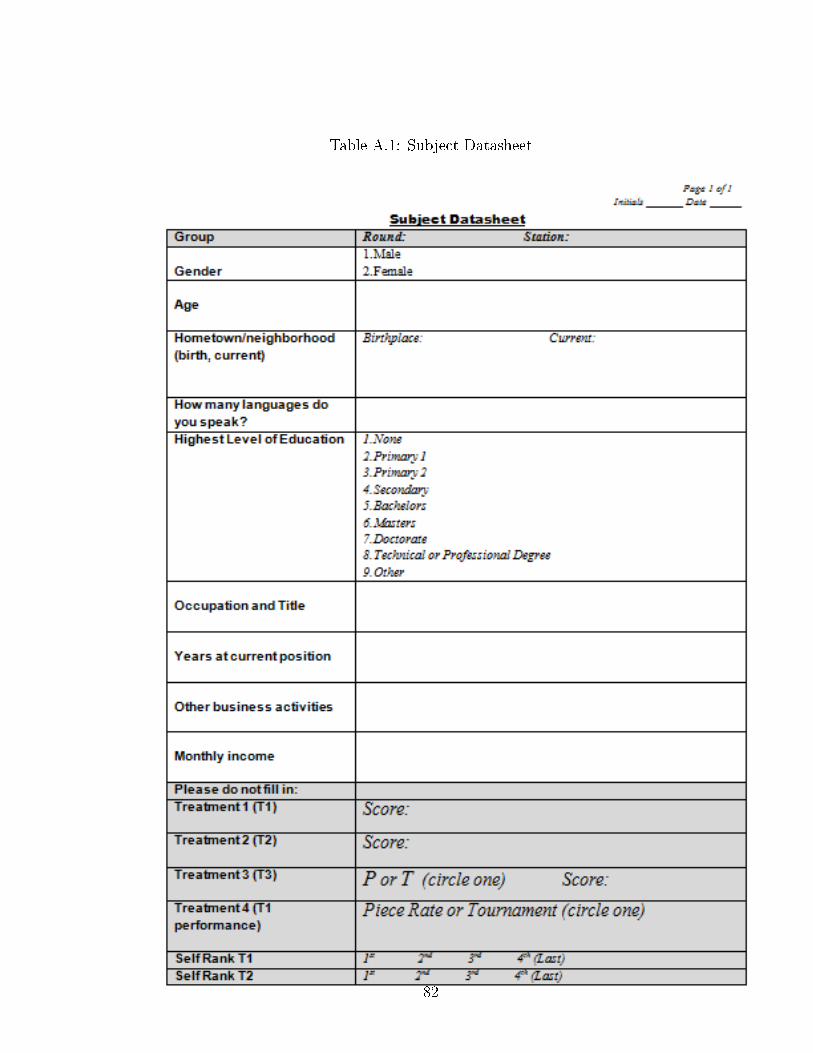
Table A.1: Subject Datasheet

82

Chapter B

Tax Evasion and Charity: Experiment Instructions

B.1 Treatment 1 Instructions

This is an experiment in decision making. Research foundations have provided funds

for conducting this research. Your earnings will depend partly on your decisions

and the decisions of the other participants and partly on chance. Please pay careful

attention to the instructions as a considerable amount of money is at stake.

The entire experiment should be complete within an hour. At the end of the

experiment you will be paid privately. At this time, you will receive $5 as a partici-

pation fee (simply for showing up on time). Details of how you will make decisions

and receive payments will be provided below.

A Decision Problem: In this experiment, you will participate in 20 independent

decision problems that share a common form. This section describes in detail the

process that will be repeated in all decision problems.

Before the beginning of the experiment, each participant will be randomly assigned

into two groups. Half of the participants will be in �Group A�, and half of the

participants will be in�Group B�. Your assigned group will stay the same throughout

the end of the experiment. At each of the 20 rounds, one participant from Group A

will be randomly matched with one participant from Group B.

83

If you are assigned to �Group A�: Each round, you will have an equal chance of

receiving an either $20 or $10. The amount you received is your private information

and known only by you. You must decide whether to disclose $20 or $10. You must

pay a portion of the money you receive back to the experimenter, which will be paid to

your Group B counterpart, depending on which amount you received: if you received

$20, you must pay back $6; if you received $10, you do not have to pay back the

experimenter. The amount immediately deducted from your account will be based

on the amount you disclose. You may disclose any amount, but if you are selected

for veri�cation, you will be subject to a penalty if your disclosure does not match

the actual amount you received. You will also have the option to donate $3 from

the money you have received to the Maryland Fund for Excellence. If you choose to

donate to charity, your donation will be subtracted from the money you have received

and will have no impact on the amount you must pay back to the experimenter.

Veri�cation

Each round, you will be paired with a di�erent participant at random from Group

B who may choose to verify your reported income. If your income report is chosen

for veri�cation and you have misreported your income, you will pay the experimenter

the amount required based on your actual income plus a penalty of $6.

Below you can �nd your payo�s under each possible scenario,

At the end of each round, you will learn whether your partner decided to verify

your income or not.

If you are assigned to �Group B�: Each round, you will be paired with a di�erent

participant at random from Group A. You will learn his/her reported income and

his/her actual charity donation to the Maryland Fund for Excellence. His/her re-

ported income will determine how much he/she pays to the experimenter, which will

be in turn given to you. After learning this information, you will be asked whether

84

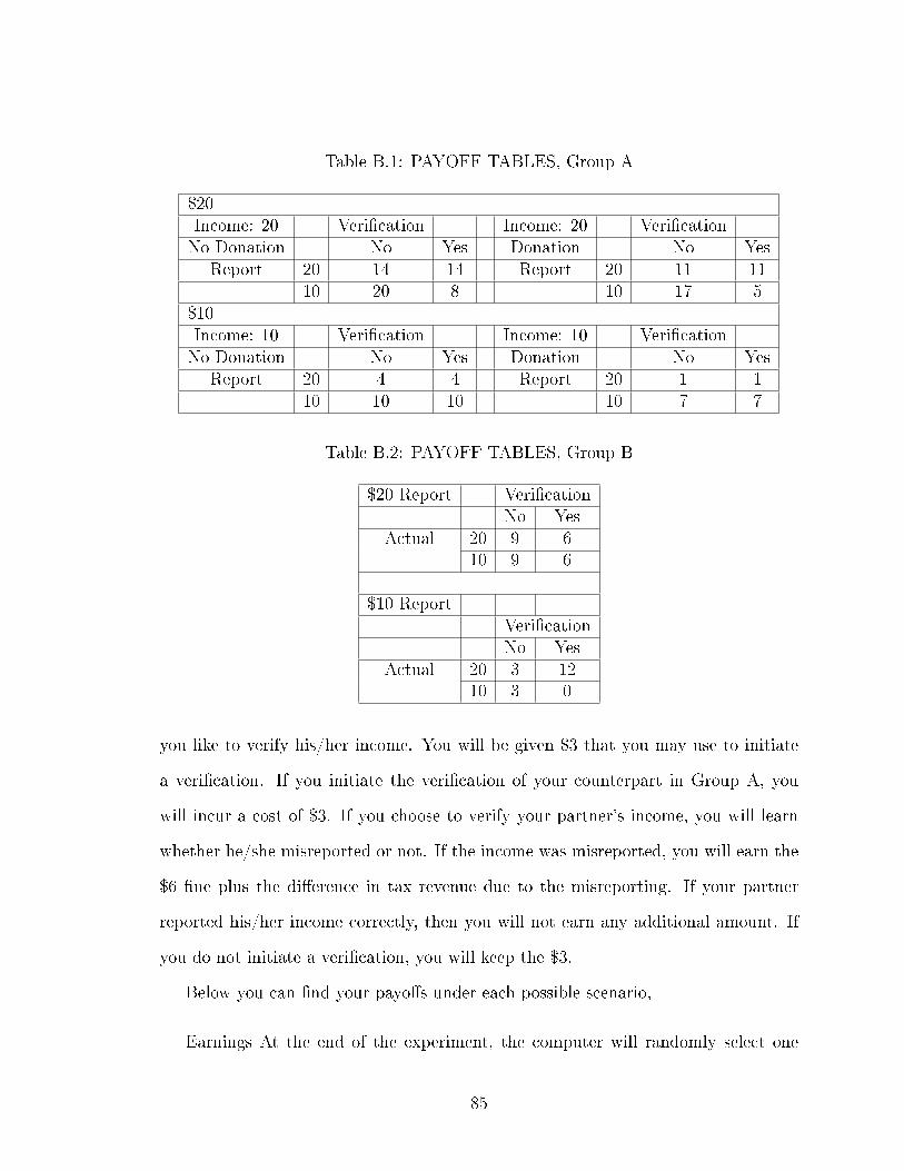
Table B.1: PAYOFF TABLES, Group A

$20Income: 20 Veri�cation Income: 20 Veri�cationNo Donation No Yes Donation No Yes

Report 20 14 14 Report 20 11 1110 20 8 10 17 5

$10Income: 10 Veri�cation Income: 10 Veri�cationNo Donation No Yes Donation No Yes

Report 20 4 4 Report 20 1 110 10 10 10 7 7

Table B.2: PAYOFF TABLES, Group B

$20 Report Veri�cationNo Yes

Actual 20 9 610 9 6

$10 ReportVeri�cationNo Yes

Actual 20 3 1210 3 0

you like to verify his/her income. You will be given $3 that you may use to initiate

a veri�cation. If you initiate the veri�cation of your counterpart in Group A, you

will incur a cost of $3. If you choose to verify your partner's income, you will learn

whether he/she misreported or not. If the income was misreported, you will earn the

$6 �ne plus the di�erence in tax revenue due to the misreporting. If your partner

reported his/her income correctly, then you will not earn any additional amount. If

you do not initiate a veri�cation, you will keep the $3.

Below you can �nd your payo�s under each possible scenario,

Earnings At the end of the experiment, the computer will randomly select one

85

decision round. Each round is equally likely to be selected.

Rules: All information will be kept secret and only the researchers will have access

to it. Your decision to play or not play will have absolutely no impact on your course

grades or employment and all data we collect will be anonymous. If you decide not

to participate in this study or if you stop participating at any time, you will not be

penalized or lose any bene�ts to which you otherwise qualify. Please do not talk with

anyone during the experiment. We ask everyone to remain silent until the end of the

last round. If there are no further questions, you are ready to start.

B.2 Treatment 2 Instructions

This is an experiment in decision making. Research foundations have provided funds

for conducting this research. Your earnings will depend partly on your decisions

and the decisions of the other participants and partly on chance. Please pay careful

attention to the instructions as a considerable amount of money is at stake.

The entire experiment should be completed within an hour. At the end of the

experiment you will be paid privately. At this time, you will receive $5 as a partici-

pation fee (simply for showing up on time). Details of how you will make decisions

and receive payments will be provided below.

A Decision Problem: In this experiment, you will participate in 20 independent

decision problems that share a common form. This section describes in detail the

process that will be repeated in all decision problems.

Before the beginning of the experiment, each participant will be randomly assigned

into two groups. Half of the participants will be in �Group A�, and half of the

participants will be in �Group B�. Your assigned group will stay the same throughout

86

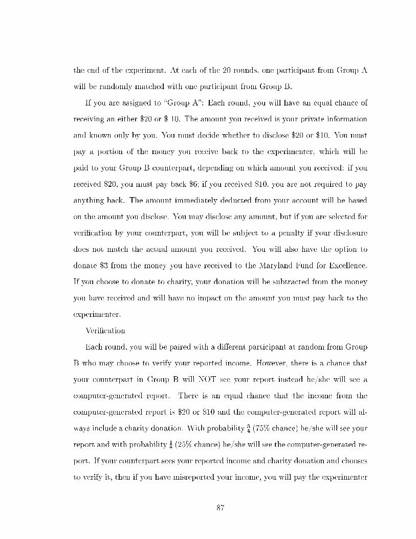
the end of the experiment. At each of the 20 rounds, one participant from Group A

will be randomly matched with one participant from Group B.

If you are assigned to �Group A�: Each round, you will have an equal chance of

receiving an either $20 or $ 10. The amount you received is your private information

and known only by you. You must decide whether to disclose $20 or $10. You must

pay a portion of the money you receive back to the experimenter, which will be

paid to your Group B counterpart, depending on which amount you received: if you

received $20, you must pay back $6; if you received $10, you are not required to pay

anything back. The amount immediately deducted from your account will be based

on the amount you disclose. You may disclose any amount, but if you are selected for

veri�cation by your counterpart, you will be subject to a penalty if your disclosure

does not match the actual amount you received. You will also have the option to

donate $3 from the money you have received to the Maryland Fund for Excellence.

If you choose to donate to charity, your donation will be subtracted from the money

you have received and will have no impact on the amount you must pay back to the

experimenter.

Veri�cation

Each round, you will be paired with a di�erent participant at random from Group

B who may choose to verify your reported income. However, there is a chance that

your counterpart in Group B will NOT see your report instead he/she will see a

computer-generated report. There is an equal chance that the income from the

computer-generated report is $20 or $10 and the computer-generated report will al-

ways include a charity donation. With probability ¾ (75% chance) he/she will see your

report and with probability ¼ (25% chance) he/she will see the computer-generated re-

port. If your counterpart sees your reported income and charity donation and chooses

to verify it, then if you have misreported your income, you will pay the experimenter

87

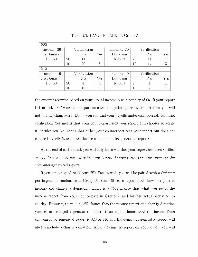
Table B.3: PAYOFF TABLES, Group A

$20Income: 20 Veri�cation Income: 20 Veri�cationNo Donation No Yes Donation No Yes

Report 20 14 14 Report 20 11 1110 20 8 10 17 5

$10Income: 10 Veri�cation Income: 10 Veri�cationNo Donation No Yes Donation No Yes

Report 20 4 4 Report 20 1 110 10 10 10 7 7

the amount required based on your actual income plus a penalty of $6. If your report

is truthful, or if your counterpart sees the computer-generated report then you will

not pay anything extra. Below you can �nd your payo�s under each possible scenario;

veri�cation Yes means that your counterpart sees your report and chooses to verify

it; veri�cation No means that either your counterpart sees your report but does not

choose to verify it or he/she has sees the computer-generated report:

At the end of each round, you will only learn whether your report has been veri�ed

or not. You will not learn whether your Group B counterpart saw your report or the

computer-generated report.

If you are assigned to �Group B�: Each round, you will be paired with a di�erent

participant at random from Group A. You will see a report that shows a report of

income and charity a donation. There is a 75% chance that what you see is the

income report from your counterpart in Group A and his/her actual donation to

charity. However, there is a 25% chance that the income report and charity donation

you see are computer generated. There is an equal chance that the income from

the computer-generated report is $20 or $10 and the computer-generated report will

always include a charity donation. After viewing the report on your screen, you will

88

Table B.4: PAYOFF TABLES, Group B$20 Report Computer Generated

Veri�cation Veri�cationNo Yes No Yes

Actual 20 9 6 9 610 9 6 NA NA

$10 Report Computer GeneratedVeri�cation Veri�cationNo Yes No Yes

Actual 20 3 12 NA NA10 3 0 3 0

be asked whether you would like to verify the income report. You will be given $3

that you may use to initiate a veri�cation. If you initiate the veri�cation of your

counterpart in group A, you will incur a cost of $3. If you choose to verify your

partner's income, you will learn whether he/she misreported or not. If the income

was misreported, you will earn the $6 �ne plus the di�erence in tax revenue due to

the misreporting. If your partner reported his/her income correctly or the report you

chose to verify is a computer generated report, then you will not earn any additional

amount. If you do not initiate a veri�cation, you will keep the $3.

Below you can �nd your payo�s under each possible scenario when the report you

saw was submitted by your counterpart or was computer-generated:

Earnings At the end of the experiment, the computer will randomly select one

decision round do determine your payment. Each round is equally likely to be selected.

Rules: All information will be kept secret and only the researchers will have access

to it. Your decision to play or not play will have absolutely no impact on your course

grades or employment and all data we collect will be anonymous. If you decide not

to participate in this study or if you stop participating at any time, you will not be

penalized or lose any bene�ts to which you otherwise qualify. Please do not talk with

89

anyone during the experiment. We ask everyone to remain silent until the end of the

last round. If there are no further questions, you are ready to start.

90

Bibliography

Akerlof, G. A. and R. E. Kranton (2000, August). Economics and identity. The

Quarterly Journal of Economics 115 (3), 715�753.

Aldous, J. (1962). Urbanization, the extended family, and kinship ties in west africa.

Social Forces 41 (1).

Allingham, M. G. and A. Sandmo (1972). Income tax evasion: A theoretical analysis.

Journal of Public Economics 1, 323�338.

Alm, J., B. Jackson, and M. McKee (1992a). Institutional uncertainty and taxpayer

compliance. American Economic Review 82 (4), 1018�1026.

Alm, J., B. R. Jackson, and M. McKee (1992b). Estimating the determinants of

taxpayer compliance with experimental data. National Tax Journal 45 (1), 107�

114.

Alm, J., B. R. Jackson, and M. McKee (2009). Getting the word out: Enforcement in-

formation dissemination and compliance behavior. Journal of Public Economics 93,

392�402.

Alm, J. and M. McKee (2004). Tax compliance as a coordination game. Journal of

Economic Behavior and Organization 54, 297�312.

Amin, M. (2010). Obstacles to Registering: Necessity vs. Opportunity Entrepreneurs.

SSRN eLibrary .

91

Androeni, J. (1990). Impure altruism and donations to public goods: A theory of

warm-glow giving. The Economic Journal 100 (401), 464�477.

Androeni, J. and R. Petrie (2004). Public goods experiments without con�dentiality:

a glimpse into fund-raising. Journal of Public Economics 88, 1605�1623.

Bank, W. (2009). World bank country data pro�les. Online; accessed April-2009.

Bassetto, M. and C. Phelan (2008, 07). Tax riots. Review of Economic Studies 75 (3),

649�669.

Baumol, W. J. (1990, October). Entrepreneurship: Productive, unproductive, and

destructive. Journal of Political Economy 98 (5), 893�921.

Becker, G. S. (1968). Crime and punishment: An economic approach. Journal of

Political Economy 76, 169.

Bernard Fortin, G. L. and M.-C. Villeval (2007). Tax evasion and social interactions.

Journal of Public Economics 91, 2089�2112.

Bernasconi, M. (1998). Tax evasion and orders of risk aversion. Journal of Public

Economics 67, 123�134.

Bewley, T. (1989). Market innovation and entrepreneurship: a knightian view. Cowles

Foundation Discussion Paper (No. 905).

Blanch�ower, D. and A. Oswald (1993, March). Entrepreneurship. CEP Discussion

Papers dp0134, Centre for Economic Performance, LSE.

Boakye-Yiadom, L. (2004). The evolution of welfare in ghana: A rural-urban per-

spective. International Conference on Ghana's Economy at the Half Century Accra,

Ghana, July 18-20, 2004.

92

Bradshaw, Y. (1987). Urbanization and underdevelopment: A global study of mod-

ernization, urban bias, and economic dependency. American Sociological Review 52,

224�239.

Brandts, J. and C. A. Holt (1992, December). An experimental test of equilibrium

dominance in signaling games. American Economic Review 82 (5), 1350�65.

Bull, C., A. Schotter, and K. Weigelt (1987). Tournaments and piece rates: An

experimental study. Journal of Political Economy 95 (1), 1�33.

Busenitz, L. (1999). Entrepreneurial risk and strategic decision making: It's a matter

of perspective. The Journal of Applied Behavioral Science 35, 325�340.

Cadsby, C. B., M. Frank, and V. Maksimovic (1990). Pooling, separating, and

semiseparating equilibria in �nancial markets: Some experimental evidence. Review

of Financial Studies 3 (3), 315�42.

Cadsby, C. B., M. Frank, and V. Maksimovic (1998). Equilibrium dominance in

experimental �nancial markets. Review of Financial Studies 11 (1), 189�232.

Camerer, C. and K. Weigelt (1988). Experimental tests of a sequential equilibrium

reputation model. Econometrica 56 (1), 1�36.

Carpenter, J. and E. Seki (2005, July). Competitive work environments and social

preferences: Field experimental evidence from a japanese �shing community. IZA

Discussion Papers 1691, Institute for the Study of Labor (IZA).

Cohen, W. and D. Levinthal (1990). Absorptive capacity: A new perspective on

learning and innovation. Administrative Science Quarterly 35 (1), 128�152.

Cooper, D. J. and J. H. Kagel (2003, March). The impact of meaningful context

93

on strategic play in signaling games. Journal of Economic Behavior & Organiza-

tion 50 (3), 311�337.

Corbridge, S. and G. Jones (2005). The continuing debate about urban bias: the

thesis, its critics, its in�uence, and implications for poverty reduction. Department

of Geography and Environment, London School of Economics and Political Science,

London, UK .

Corporation, I. F. (2008, September). Ifc program supports 10,000 entrepreneurs in

33 african countries.

De Soto, H. (2000). The Mystery of Capital. New York: Basic Books.

Deneckere, R. and M.-Y. Liang (2010). Tea parties.

Djankov, S., R. L. Porta, F. Lopez-De-Silanes, and A. Shleifer (2002, February). The

regulation of entry. The Quarterly Journal of Economics 117 (1), 1�37.

Du�y, J. and N. Feltovich (2006, 07). Words, deeds, and lies: Strategic behaviour in

games with multiple signals. Review of Economic Studies 73 (3), 669�688.

Eastwood, R. and M. Lipton (2000). Rural-urban dimensions of inequality change.

World Institute for Development Economics Research (WIDER) Working Pa-

per (No. 200).

Erev, I. and A. E. Roth (1998). Predicting how people play games: Reinforcement

learning in experimental games with unique, mixed strategy equilibria. The Amer-

ican Economic Review 88 (4), pp. 848�881.

Farrell, J. and M. Rabin (1996, Summer). Cheap talk. Journal of Economic Perspec-

tives 10 (3), 103�18.

94

Fehr, E. and S. Gaechter (2000). Cooperation and punishment in public goods ex-

periments. The American Economic Review 90 (4), pp. 980�994.

Fischbacher, U. (2007, June). z-tree: Zurich toolbox for ready-made economic exper-

iments. Experimental Economics 10 (2), 171�178.

Forsythe, R., R. Lundholm, and T. Rietz (1999). Cheap talk, fraud, and adverse

selection in �nancial markets: Some experimental evidence. Review of Financial

Studies 12 (3), 481�518.

Geschiere, P. and J. Gugler (1998). Introduction: The urban-rural connection:

Changing issues of belonging and identi�cation. Africa: Journal of the Interna-

tional African Institute, The Politics of Primary Patriotism 68 (3), 309�319.

Gneezy, U. (2005). Deception: The role of consequences. American Economic Re-

view 95 (1), 384�394.

Gneezy, U., K. L. Leonard, and J. A. List (2009, 09). Gender di�erences in competi-

tion: Evidence from a matrilineal and a patriarchal society. Econometrica 77 (5),

1637�1664.

Graetz, M. J., J. F. Reinganum, and L. L. Wilde (1986, Spring). The tax compliance

game: Toward an interactive theory of law enforcement. Journal of Law, Economics

and Organization 2 (1), 1�32.

Gupta, N. D., A. Poulsen, and A.-C. Villeval (2005, November). Male and female

competitive behavior: Experimental evidence. IZA Discussion Papers 1833, Insti-

tute for the Study of Labor (IZA).

Hillman, A. L., N. Van Long, and A. Soubeyran (2001, August). Protection, lobbying,

and market structure. Journal of International Economics 54 (2), 383�409.

95

Hsu, L.-C. (2006). Experimental evidence on tax compliance and voluntary public

good provision. National Chengchi University.

Johnson, S., D. Kaufmann, and P. Zoido-Lobaton (1998, May). Regulatory discretion

and the uno�cial economy. American Economic Review 88 (2), 387�92.

Kihlstrom, R. and J.-J. La�ont (1979). A general equilibrium entrepreneurial theory

of �rm formation based on risk aversion. Journal of Political Economy 87, 719�848.

Kim, C. K. and W. S. Waller (2005). A Behavioral Accounting Study of Strategic

Interaction in a Tax Compliance Game, Volume III. Netherlands: Springer.

Klapper, L., L. Laeven, and R. Rajan (2006, December). Entry regulation as a barrier

to entrepreneurship. Journal of Financial Economics 82 (3), 591�629.

Lazear, E. (2005). Entrepreneurship. Journal of Labor EconomicsJournal of Labor

Economics 23 (4), 649�680.

Lazear, E. P. and S. Rosen (1981, October). Rank-order tournaments as optimum

labor contracts. Journal of Political Economy 89 (5), 841�64.

Le�, N. H. (1979, March). Entrepreneurship and economic development: The problem

revisited. Journal of Economic Literature 17 (1), 46�64.

Lipton, M. (1977). Why Poor People Stay Poor: Urban Bias in World Development.

Cambridge: Harvard University Press.

Makura, M. (2008). Africa's greatest entrepreneursl. Johannesburg: Penguin Books

South Africa.

Max Albert, Werner Güth, E. K. and B. Maciejovsky (2007). Are we nice (r) to nice

(r) people?-an experimental analysis. Experimental Ecoomics 10 (1), 53�69.

96

Moore, D. A. and D. A. Small (2007). Error and bias in comparative judgment: On

being both better and worse than we think we are. Journal of Personality and

Social Psychology 92 (6), 972�989.

Natarajan, L. (2005, September). Entrepreneurial optimism: Understanding market

entry decisions. Masters thesis.

Naude, W. (2008). Entrepreneurship in economic development. Technical report.

Niederle, M. and L. Vesterlund (2007, 08). Do women shy away from competition? do

men compete too much? The Quarterly Journal of Economics 122 (3), 1067�1101.

Nsowah-Nuamah, N., F. Teal, and M. Awoonor-Williams (2010). Jobs, skills and

incomes in ghana: How was poverty halved? Technical report.

Ochs, J. (1995). Games with unique, mixed strategy equilibria: An experimental

study. Games and Economic Behavior 10 (1), 202 � 217.

of the Treasury, U. D. (2009, August). Update on reducing the federal tax gap and

improving voluntary compliance.

Petrin, T. (1994). Entrepreneurship as an economic force in rural development. Tech-

nical report.

Putnam, R. D. (2000). Social capital and community benchmark survey. Saguaro

Seminar Civic Engagement in America, John F. Kennedy School of Government ,

http://www.cfsv.org/communitysurvey/index.html.

Reinganum, J. F. and L. L. Wilde (1985, February). Income tax compliance in a

principal-agent framework. Journal of Public Economics 26 (1), 1�18.

97

Reinganum, J. F. and L. L. Wilde (1986, October). Equilibrium veri�cation and

reporting policies in a model of tax compliance. International Economic Re-

view 27 (3), 739�60.

Robson, P., H. Haugh, and B. A. Obeng (2009). Entrepreneurship and innovation in

ghana: enterprising africa. Small Business Economics 32, 331�350.

Sahn, D. E. and D. C. Stifel (2004). Urban-rural inequality in living standards in

africa. Technical report.

Slemrod, J., M. Blumenthal, and C. Christian (2001, March). Taxpayer response to an

increased probability of audit: evidence from a controlled experiment in minnesota.

Journal of Public Economics 79 (3), 455�483.

Spence, A. M. (1973). Job market signaling. Quarterly Journal of Economics 87 (3),

355 � 374.

Thomas, A. S. and S. L. Mueller (2000). A case for comparative entrepreneurship:

Assessing the relevance of culture. Journal of International Business Studies 31 (2),

287�301.

UNCTAD (2009). United nations conference on trade and development, fdi statistics.

Online; accessed July-2009.

UNEP/GRID-Arendal (2009). Globalis. Online; accessed April-2009.

van der Sluis, J., M. van Praag, and W. Vijverberg (2005). Entrepreneurship selec-

tion and performance: A meta-analysis of the impact of education in developing

economies. World Bank Economic Review 19 (2), 225�261.

Varshney, A. (Ed.) (1993). Beyond Urban Bias. London: Frank Cass.

98