DISSERTATION ESSAYS ON FISCAL DECENTRALIZATION AND …

DISSERTATION

ESSAYS ON FISCAL DECENTRALIZATION AND TAXATION

Submitted by

Ardyanto Fitrady

Department of Economics

In partial fulfillment of the requirements

For the Degree of Doctor of Philosophy

Colorado State University

Fort Collins, Colorado

Summer 2014

Doctoral Committee:

Advisor: Harvey CutlerCo-Advisor: Anita Alves Pena

David MushinskiStephan Kroll

Copyright by Ardyanto Fitrady 2014

All Rights Reserved

ABSTRACT

ESSAYS ON FISCAL DECENTRALIZATION AND TAXATION

This dissertation investigates two important topics in economics. First, the impacts

of spillovers of public goods on the potential benefits from decentralization in an urban

economy. Second, the role of tax evasion and uncertainty on the optimal taxation for two-

class economy.

Theoretical model and numerical simulations are used to study the first topic in

Chapter 2. The results from the numerical simulation shows that the spillover level has

an impact on the potential gain of decentralization. The general results of the numeri-

cal simulations demonstrate that as the degree of spillovers increases, the potential gain of

decentralization over centralization diminishes in both cases of metropolitan areas in de-

veloped and developing countries. These results celebrate Oates’ decentralization theorem

where decentralization is more beneficial when spillovers among jurisdictions are relatively

low. However, the result also shows that the impact of the spillover level on the potential

gain of decentralization varies across different levels of income vis-a-vis income inequality. It

shows that a metropolitan area with lower mean income will be suffer more from the spillover

than a metropolitan area with higher mean income. The numerical simulation also shows

that a higher level of inequality amplifies the benefit of decentralization. It illustrates that

the developed country—in this case the United States—that generally has higher income

inequality, potentially gains more benefits from decentralization.

ii

Theoretical models are used in Chapter 3 to examine the importance of tax evasion

in the optimal taxation theory that are built based on previous studies. Although one can

find that most of the results are intuitive, the model shows that considering tax evasion and

uncertainty is important in implementing tax policies, particularly in the process of setting

the tax rates for income tax and sales tax. The income tax for the high-type individual will

be higher as the degree of tax evasion increases and the income tax of the low-type individual

decreases as the probability of being detected for the high-type increases, ceteris paribus.

The result also shows that the optimal income tax rate for the low-type individual increases

as the marginal utility of mimicking the low type or the marginal utility of income for the

mimicker increases, ceteris paribus. In other words, income tax for the low-type will increase

if the high type has more incentive to mimic the low-type.

iii

ACKNOWLEDGMENTS

First of all, I would like to thank my family. Most of all, my beloved wife Dian, and

our dearly loved sons Saka and Arana whose love and patience support me for all the years I

spent in pursuing my doctoral degree and still continue until today. I also thank my parents

for their endless support and prayers they have provided me throughout my life.

I am a very grateful to my advisor Harvey Cutler his guidance and supports in my

dissertation along with his noteworthy patience. He was always available for discussion over

the development of this dissertation. My deep gratitude, appreciation, and respect go to my

co-advisor Anita Alves Pena for her insightful advice, constructive comments, and remarkable

kindness. I cannot thank you enough. Thank you to David Mushinski and Stephan Kroll

for their valuable time and constructive comments. Many elements of my dissertation were

improved through discussions with them.

Many thanks to all my professors in the Economics Department from whom I learned

a lot, especially Alexandra Bernasek and Robert Kling who are always willing to provide

advices in my early years as a graduate student. Special thanks to Barbara Alldredge,

Brooke Taylor, and Jenifer Davis for their dedication to the success of graduate students in

the Department of Economics, Colorado State University.

I would also like to express my gratitude and thanks to the Faculty of Economics and

Business, Universitas Gadjah Mada that has supported me in my last year in Ph.D. program.

iv

Last but not least, I would like to offer my sincerest thanks to all my friends in the

United States and Indonesia who have supported me throughout of my academic life in

Colorado State University.

While all contributions helped enormously in the process of this dissertation, any

errors are my own.

v

TABLE OF CONTENTS

Chapter 1. Introduction . . . . . . . . . . . . . . . . . . . . . . . . . . . . . . . . . 1

Chapter 2. Fiscal Decentralization, Local Public Goods, and Welfare of Cities . . . 5

2.1 Introduction . . . . . . . . . . . . . . . . . . . . . . . . . . . . . . . . . . . . 5

2.1.1 Background . . . . . . . . . . . . . . . . . . . . . . . . . . . . . . . . 5

2.1.2 Research questions . . . . . . . . . . . . . . . . . . . . . . . . . . . . 7

2.1.3 Research outline . . . . . . . . . . . . . . . . . . . . . . . . . . . . . 8

2.2 Literature Review . . . . . . . . . . . . . . . . . . . . . . . . . . . . . . . . . 9

2.2.1 Economics of cities and equilibrium . . . . . . . . . . . . . . . . . . . 10

2.2.2 Fiscal decentralization . . . . . . . . . . . . . . . . . . . . . . . . . . 15

2.2.3 Local public goods and Pareto optimum . . . . . . . . . . . . . . . . 23

2.2.4 Summary . . . . . . . . . . . . . . . . . . . . . . . . . . . . . . . . . 28

2.3 The Model . . . . . . . . . . . . . . . . . . . . . . . . . . . . . . . . . . . . . 29

2.3.1 Settings . . . . . . . . . . . . . . . . . . . . . . . . . . . . . . . . . . 29

2.3.2 Characterization of Pareto optimum . . . . . . . . . . . . . . . . . . 31

2.4 Numerical Simulations: Welfare change and equilibria . . . . . . . . . . . . . 34

2.4.1 Methodology . . . . . . . . . . . . . . . . . . . . . . . . . . . . . . . 35

2.4.2 Data and utility function . . . . . . . . . . . . . . . . . . . . . . . . . 36

2.4.3 A case of an urban economy in the United States . . . . . . . . . . . 37

2.4.3.1 Calibrations and results . . . . . . . . . . . . . . . . . . . . 37

vi

2.4.4 A case of an urban economy in Indonesia . . . . . . . . . . . . . . . . 45

2.4.4.1 Calibrations and results . . . . . . . . . . . . . . . . . . . . 45

2.4.5 Summary . . . . . . . . . . . . . . . . . . . . . . . . . . . . . . . . . 52

2.5 Numerical Simulations: Income level, inequality, and welfare change . . . . . 53

2.5.1 Income and welfare change . . . . . . . . . . . . . . . . . . . . . . . . 53

2.5.2 Inequality and welfare change . . . . . . . . . . . . . . . . . . . . . . 55

2.5.3 A higher degree of spillovers and switching to centralization . . . . . 57

2.5.4 Summary . . . . . . . . . . . . . . . . . . . . . . . . . . . . . . . . . 59

2.6 Conclusions and policy implications . . . . . . . . . . . . . . . . . . . . . . . 60

Chapter 3. Optimal Income-Sales Taxation, Tax Evasion, and Uncertainty . . . . . 63

3.1 Introduction . . . . . . . . . . . . . . . . . . . . . . . . . . . . . . . . . . . . 63

3.1.1 Background . . . . . . . . . . . . . . . . . . . . . . . . . . . . . . . . 63

3.1.2 Research questions . . . . . . . . . . . . . . . . . . . . . . . . . . . . 64

3.1.3 Research outline . . . . . . . . . . . . . . . . . . . . . . . . . . . . . 65

3.2 Literature Review . . . . . . . . . . . . . . . . . . . . . . . . . . . . . . . . . 65

3.2.1 Commodity taxation . . . . . . . . . . . . . . . . . . . . . . . . . . . 66

3.2.2 Income taxation . . . . . . . . . . . . . . . . . . . . . . . . . . . . . . 67

3.2.3 Direct-indirect taxation . . . . . . . . . . . . . . . . . . . . . . . . . 69

3.2.4 Summary . . . . . . . . . . . . . . . . . . . . . . . . . . . . . . . . . 74

3.3 The Model . . . . . . . . . . . . . . . . . . . . . . . . . . . . . . . . . . . . . 75

3.3.1 Assumptions . . . . . . . . . . . . . . . . . . . . . . . . . . . . . . . . 75

3.3.2 The household’s maximization problem . . . . . . . . . . . . . . . . . 76

vii

3.3.3 The mimicker’s maximization problem . . . . . . . . . . . . . . . . . 77

3.3.4 The social planner’s problem . . . . . . . . . . . . . . . . . . . . . . . 78

3.4 Conclusions and policy implications . . . . . . . . . . . . . . . . . . . . . . . 82

Chapter 4. Concluding Remarks . . . . . . . . . . . . . . . . . . . . . . . . . . . . 85

Bibliography . . . . . . . . . . . . . . . . . . . . . . . . . . . . . . . . . . . . . . . . 96

Appendices . . . . . . . . . . . . . . . . . . . . . . . . . . . . . . . . . . . . . . . . . 97

A.1 Derivations of First-order conditions . . . . . . . . . . . . . . . . . . . . 97

A.2 Deriving equations for MATLAB functions . . . . . . . . . . . . . . . . . 100

A.3 Matlab codes . . . . . . . . . . . . . . . . . . . . . . . . . . . . . . . . . 114

A.4 Comparison between Monte Carlo and Quadrature Results . . . . . . . . 147

A.5 The household’s maximization problem . . . . . . . . . . . . . . . . . . 149

A.6 The mimicker’s maximization problem . . . . . . . . . . . . . . . . . . . 151

A.7 The planner’s problem . . . . . . . . . . . . . . . . . . . . . . . . . . . . 153

viii

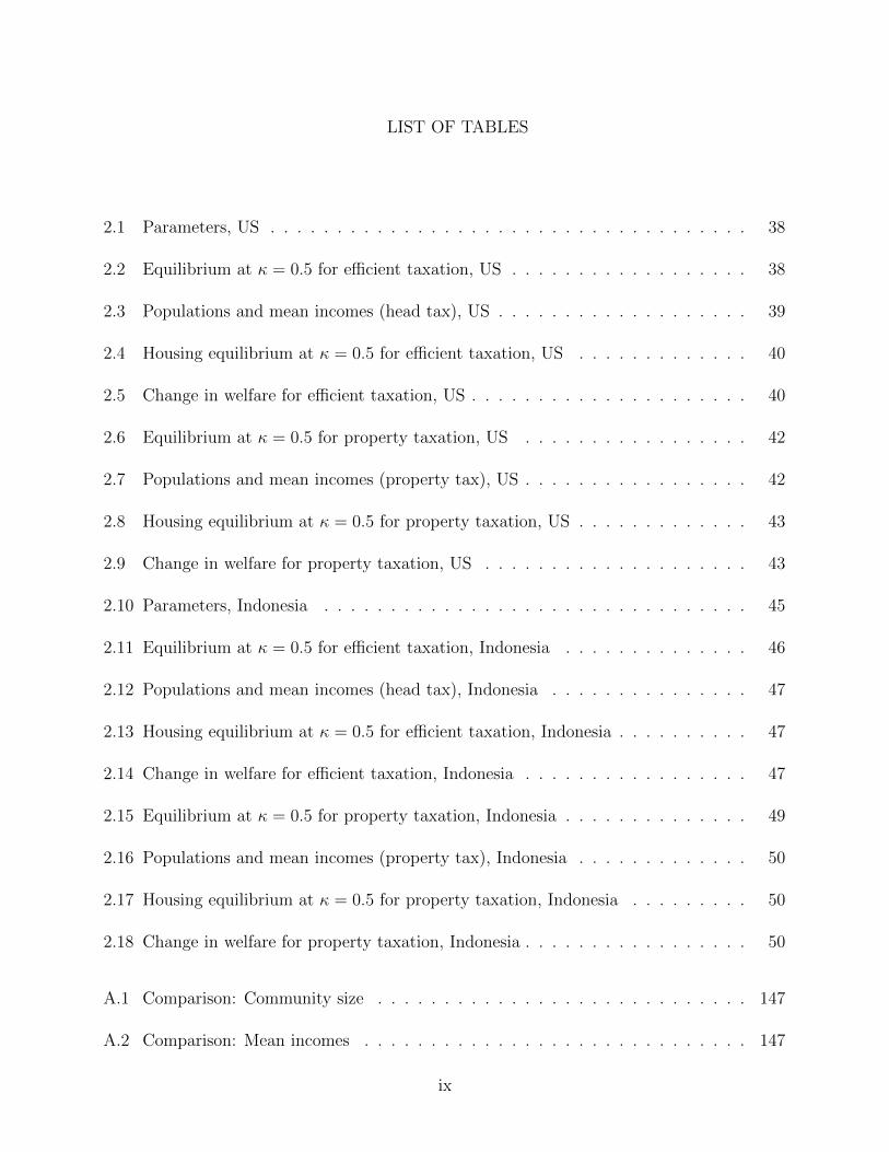
LIST OF TABLES

2.1 Parameters, US . . . . . . . . . . . . . . . . . . . . . . . . . . . . . . . . . . . . 38

2.2 Equilibrium at κ = 0.5 for efficient taxation, US . . . . . . . . . . . . . . . . . . 38

2.3 Populations and mean incomes (head tax), US . . . . . . . . . . . . . . . . . . . 39

2.4 Housing equilibrium at κ = 0.5 for efficient taxation, US . . . . . . . . . . . . . 40

2.5 Change in welfare for efficient taxation, US . . . . . . . . . . . . . . . . . . . . . 40

2.6 Equilibrium at κ = 0.5 for property taxation, US . . . . . . . . . . . . . . . . . 42

2.7 Populations and mean incomes (property tax), US . . . . . . . . . . . . . . . . . 42

2.8 Housing equilibrium at κ = 0.5 for property taxation, US . . . . . . . . . . . . . 43

2.9 Change in welfare for property taxation, US . . . . . . . . . . . . . . . . . . . . 43

2.10 Parameters, Indonesia . . . . . . . . . . . . . . . . . . . . . . . . . . . . . . . . 45

2.11 Equilibrium at κ = 0.5 for efficient taxation, Indonesia . . . . . . . . . . . . . . 46

2.12 Populations and mean incomes (head tax), Indonesia . . . . . . . . . . . . . . . 47

2.13 Housing equilibrium at κ = 0.5 for efficient taxation, Indonesia . . . . . . . . . . 47

2.14 Change in welfare for efficient taxation, Indonesia . . . . . . . . . . . . . . . . . 47

2.15 Equilibrium at κ = 0.5 for property taxation, Indonesia . . . . . . . . . . . . . . 49

2.16 Populations and mean incomes (property tax), Indonesia . . . . . . . . . . . . . 50

2.17 Housing equilibrium at κ = 0.5 for property taxation, Indonesia . . . . . . . . . 50

2.18 Change in welfare for property taxation, Indonesia . . . . . . . . . . . . . . . . . 50

A.1 Comparison: Community size . . . . . . . . . . . . . . . . . . . . . . . . . . . . 147

A.2 Comparison: Mean incomes . . . . . . . . . . . . . . . . . . . . . . . . . . . . . 147

ix

A.3 Comparison: Mean housing demand . . . . . . . . . . . . . . . . . . . . . . . . . 147

A.4 Comparison: Community size . . . . . . . . . . . . . . . . . . . . . . . . . . . . 148

A.5 Comparison: Mean incomes . . . . . . . . . . . . . . . . . . . . . . . . . . . . . 148

A.6 Comparison: Housing demand . . . . . . . . . . . . . . . . . . . . . . . . . . . . 148

x

LIST OF FIGURES

2.1 Welfare loss from centralization: variations in demand . . . . . . . . . . . . . . . 16

2.2 Spillover and potential gain of decentralization in head-tax world, US . . . . . . 40

2.3 Spillover and potential gain of decentralization in property-tax world, US . . . . 44

2.4 Spillover and potential gain of decentralization in head-tax world, Indonesia . . 48

2.5 Spillover and potential gain of decentralization in property-tax world, Indonesia 51

2.6 Income level and welfare change at various degrees of spillover, US . . . . . . . . 54

2.7 Inequality and welfare change at various degrees of spillover, US . . . . . . . . . 56

2.8 Potential gain from decentralization in the head-tax world, US . . . . . . . . . . 58

2.9 Potential gain from decentralization in the property-tax world, Indonesia . . . . 59

xi

CHAPTER 1

Introduction

This dissertation focuses on frameworks of two important topics in public economics,

i.e. urban fiscal decentralization and optimal taxation. Discourses on both topics are impor-

tant in public and urban economics, implying that there are always possibilities to improve

the existing theory with different methods and assumptions. Both theoretical and numerical

approaches will be used to investigate the important aspects of urban fiscal decentralization.

It is not the purpose of this dissertation to change fundamental understandings of existing

theory or models. Instead, it focuses more on contributing to the existing model or theory by

introducing new variables into the models. Parallel results will enrich the existing theory by

demonstrating some robustness of the model as new variables are introduced in the model.

The second chapter discusses fiscal decentralization in an urban area where the au-

thority to provide local public goods, as well as the taxation to finance the provision, can

be centralized in one large jurisdiction or decentralized into two small jurisdictions or more.

The debate on this issue lies on two main views of fiscal decentralization. First, fiscal decen-

tralization will benefit the economy in the aggregate. This idea is mostly based on Oates’

fiscal decentralization theorem (1972). Second, fiscal decentralization is not better than cen-

tralization. This idea is based on the belief that the effect of spillovers offsets the benefits

generated by fiscal decentralization as in Besley and Coate (2003). Moreover, when there is

no spillover in the economy, Calabrese et al. (2012) find that centralized tax policy is better

than decentralized tax policy.

1

Pareto optimum characterizations with spillovers1in urban settings are presented in

Chapter 2. Following utilitarian economics, the optimal solution of the model is solved by

maximizing total welfare of agents in the economy with three main constraints: housing

market equilibrium, government balanced budget, and balanced-budget transfer; while con-

sidering spillovers among jurisdictions. As expected, the Pareto optimum characterization

are not analytically solvable that leads to numerical simulations in the next section.

The next section in Chapter 2 conducts the empirical study using numerical sim-

ulations. By utilizing the model, assuming some parameters in the model, and employing

empirical data, we calibrate the model in order to reach the equilibrium. Cases of urban areas

in the United States and Indonesia (as a comparison of developed and developing economies)

are used to illustrate two different empirical cases. We also use two types of taxation in the

numerical simulations, i.e. efficient tax (head tax) and property tax to analyze the difference

between both cases. Estimations have been made to gauge whether the benefits from fiscal

decentralization dominates the costs when spillovers across jurisdictions are present.

The results from the numerical simulation shows that the spillover level has an impact

on the potential gain of decentralization. The general results of the numerical simulations

demonstrate that as the degree of spillovers increases, the potential gain of decentralization

diminishes in both cases of metropolitan areas in developed and developing countries. These

results celebrate Oates’ decentralization theorem where decentralization is more beneficial

when spillovers among jurisdictions are relatively low due to the optimal levels of local public

good provisions.

1In this research, spillover is defined as a positive externality of local public goods in a certain jurisdictionto households’ utility in other jurisdictions. We assume that there is no negative externality in the economyfrom local public good provision.

2

However, the result also shows that the impact of the spillover level on the potential

gain of decentralization varies across different levels of income vis-a-vis income inequality.

It shows that a metropolitan area with a relatively low mean income will be negatively af-

fected by spillover more than a metropolitan area with a relatively high mean income. The

numerical simulation also shows that a higher level of inequality amplifies the benefit of

decentralization. It illustrates that developed countries—that generally have higher income

inequality—potentially gain more benefits from decentralization.

Chapter 3 focuses on the optimal direct-indirect taxation in the economy, particularly

income taxation and sales taxation. Related research, from Ramsey (1927) to Saez (2001),

are discussed in the literature review. The discussion is divided into three main areas: (1)

sales taxation; (2) income taxation; and (3) direct-indirect taxation. Each section focuses on

the model used and its corresponding results. This chapter contributes to popular discussion

not only to public economists but also to policy makers.

A theoretical model is built based on Nava et al. (1996) and Boadway et al. (1994)

by taking into account uncertainty and tax evasion. The modification introduces intuitive

results on the effects of tax evasion and uncertainty on income-tax and sales-tax rates. The

chapter is closed by conclusions and policy implications. Although one can find that most

of the results are intuitive, the model shows that considering tax evasion and uncertainty is

important in implementing tax policies, particularly in the process of setting the tax rates

for income tax and sales tax.

The model in Chapter 3 shows that in the Pareto optimum the sign of income tax for

the high-type agent depends on the relation between the (taxed) private good and leisure.

If the private good is a substitute for leisure, then the income tax for the high-type will be

3

negative. Conversely, if the private good is a complement for leisure, the income tax of the

high type will be positive. This result resonates the result in Nava et al. (1996). As far as

the tax evasion is concerned, the income tax for the high-type individual will be higher as

the degree of tax evasion increases. We also find that if the taxed private good and leisure

are complementary—i.e. when the income tax is positive for the high type—and the elastic-

ity of demand with respect to income tax is larger than the elasticity of labor supply with

respect to income tax, the commodity tax rate should be higher than the income tax rate

to optimize the welfare.

For the case of low-type, the model shows that the income tax of the low-type in-

dividual decreases as the probability of being detected for the high-type increases, ceteris

paribus. The result shows that the optimal income tax rate for the low-type individual in-

creases as the marginal utility of mimicking the low type or the marginal utility of income

for the mimicker increases, ceteris paribus. In other words, income tax for the low-type will

increase if the high type has more incentive to mimic the low-type. Conversely, the optimal

income tax decreases as the marginal utility of tax revenue, the number of low-type agents,

proportion of reported income, probability that the high-type will be detected when hiding

the income, or the cost of hiding the income increases.

4

CHAPTER 2

Fiscal Decentralization, Local Public Goods, and Welfare of Cities

2.1 Introduction

2.1.1 Background

The idea of fiscal decentralization or fiscal federalism1 has been started from Plato’s idea

about government in his work The Republic—one of most influential works in western phi-

losophy (Hooghe and Marks, 2007). However, a formal approach on how economists look at

the fiscal decentralization—or fiscal federalism—started in Oates’ seminal book in 1972 Fis-

cal Federalism. This literature shows that a decentralized system, under the assumption of

no spillover effects or spillovers among jurisdictions, will generate higher social welfare than

centralized system. The trade-off between those two systems depend on the heterogeneity of

preference and the degree of spillovers (Besley and Coate, 2003). Although the final result

is not really unexpected, Oates provides analysis to see this issue from economic point of

view for the first time. Many works in the literature have been written based on Oates’

fiscal decentralization theorem in the following years up to today and influence economic

and political systems widely.

The influence of fiscal decentralization brings together the idea of an ideal political

system where smaller governments should have more authority to determine the types of

goods and services that should be provided in localities and decide how to finance them. The

1In general, fiscal decentralization is the devolution by the central government to local governments(states, regions, municipalities) of specific functions with the administrative authority and fiscal revenue toperform those functions (Kee, 2004). Slightly different definition as opposed to fiscal federalism will discusslater in the literature review.

5

reasons are mainly because local governments know better about their available resources

and how to allocate the resources so the allocation will be more efficient. Moreover, local

governments know better what their people need so the allocation is expected will be more

effective.2

Samuelson (1954) asserts that there is no market solution for public good provision,

where what he means by market solution in local economy is a decentralized policy. Based

on his assertion, public goods are always under provided since there is no feasible method

to charge the consumers (Tiebout, 1956). In other words, there is no reason to believe that

public goods will be provided efficiently. This argument is criticized by Tiebout (1956). He

conjectures that competition among publicly elected governments for mobile households may

yield an efficient provision of local public goods. However, Tiebout’s hypothesis is not free

from critiques as many articles are written to argue against Tiebout’s hypothesis. We will

discuss in detail about the theory in the literature review section.

The idea of fiscal decentralization does not only have impacts on developed countries

such as the United States, but also has impacts on developing countries, such as Indonesia.

More than that, the issue is not only interesting in the context of high level of government

system such as central government versus state governments, but also in the smaller juris-

dictional system such as a metropolitan area (MA) versus cities in the corresponding MA.

Should we give the power to finance and to provide local public goods in large jurisdiction

(centralized system) or let smaller jurisdictions decide what they need to do (decentralized

system)? Here, urban economics comes into play.

2One may recall Musgrave’s three-function of government (1939): stabilization, income redistribution,and resource allocation, where the first two functions belong to the central government and the last functionbelongs to the local government.

6

Urban economic literature has a wide spectrum of discussions of decentralization

policy and spillover effects independently.3 However, to the best of my knowledge there

is no literature that specifically focuses on the discussion of fiscal decentralization where

spillover effects exist in the case of urban system. One piece of the literature focusing on

fiscal decentralization in urban area is from Calabrese et al. (2012). However, their article

discusses Tiebout equilibrium where spillovers do not exist.4 Thus, it is of interest to observe

theoretically how externalities or spillover effects will affect social welfare in a setting of

a metropolitan area. Adding the spillovers will provide an important insight into urban

economics where spillovers among jurisdictions are an essential aspect to be considered in

urban economics.

Based on the discussion above, it is very appealing to do research on this area: how

fiscal decentralization will impact social welfare via local public good provision with the

existence of spillovers among jurisdictions in the urban area? The research will be conducted

from perspectives of urban economics and public economics. A theoretical model will be built

and data for urban areas in the United States and Indonesia will be calibrated to investigate

the empirical aspects of the model.

2.1.2 Research questions

One of the most important issues in the debate of fiscal decentralization is the impact

of decentralization on social welfare. Some economists argue that decentralization will be

beneficial to society as in Oates’ decentralization theorem. In contrast, some economists

3See Oates (1972), Oates (1999), Zhang and Zou (1998), Davoodi and Zou (1998), Besley and Coate(2003), Calabrese et al. (2012) for some references.

4One of the assumptions in Tiebout (1956) is no externalities or spillovers.

7

argue that centralization is better since the spillovers among jurisdictions will not be zero.

Utilizing a political economy approach, Besley and Coate (2003) also provide that there is

some level of externalities or spillovers where decentralization will be beneficial and vice

versa.

To the best of my knowledge, none of fiscal decentralization literature points out

whether fiscal decentralization leads to a gain or a loss for the society in the context of urban

economy where the spillovers exist. Thus, the model in this dissertation is constructed to

examine that area, particularly the impact of fiscal decentralization and spillovers on the

urban welfare.

Specifically, the research questions are:

1. How can we model the impact of fiscal decentralization on social welfare when the

spillovers exist in the context of an urban economy?

2. Do the results support the existing theory?

3. Does fiscal decentralization benefit cities and society when some degree of spillover is

present?

4. Are the results consistent both in developed and developing countries?

2.1.3 Research outline

We will explore topics of fiscal decentralization, local public good provision, and their impacts

on welfare in the context of urban economics. There will be two main sections in this chapter,

i.e. the model and numerical simulations. The latter consists of two different results: (1)

comparison between urban area in developed and developing countries; and (2) impacts of

decentralization on different levels of income and inequality on the social welfare.

8

The chapter is divided into six sections. Section 2.2 will discuss literature review

on the related topics mentioned above. It will begin with the concept of economics of the

cities and equilibrium in each jurisdiction. It is then followed by the literature review in

fiscal decentralization and a discussion on the evolution of public good theory, including

Samuelson (1954), Tiebout (1956), and Bewley (1981). The chapter then is closed by a

summary leading to the theoretical model in Section 2.3.

Section 2.3 discusses the theoretical model that will explain the description of the

model and the characterization of Pareto optimum. The model is then used as bases of

computer models and numerical simulations in Section 2.4 and 2.5.

Section 2.4 discusses the calibration using data for urban area in the United States

and Indonesia. It is started with a description about the methodology, data, and assumptions

used in the simulations. It is followed by the cases of efficient and property taxation in the

United States and Indonesia that mainly focus on the welfare impacts of decentralization.

The last section in this chapter will conclude the results, compare them with previous research

and provide some policy implications.

2.2 Literature Review

This section discusses related literature that provides the underpinning theoretical framework

to construct the model and conduct the analysis. We start with discussion on economics

of cities and its equilibrium. Section 2.2.1 discusses spillover effects across jurisdictions

that potentially affect the equilibrium while Section 2.2.2 discusses some literature on fiscal

decentralization. The discussion will cover a pure economic theory from Oates (1972) and

the political economy aspect of it. The following section then will cover a discussion of local

9

public goods and welfare. This section will cover the positive approach from Musgrave (1959),

normative approach from Samuelson (1954), Tiebout hypothesis from Tiebout (1956), the

theory of clubs from Buchanan (1965), and other related literature on this topic. In the end

of this section we will summarize the literature review, explaining how it relates to the model

in this dissertation, and lead to the next section that will discuss the model in details.

2.2.1 Economics of cities and equilibrium

Urban economics is the main perspective that is used in this dissertation. Like other branches

of economics, such as in Brueckner (1986), the most challenging part in urban economics

is to construct rigorous economic explanation for a variety of observed regularities in the

structures of real-world cities. This section will discuss an economic model for a metropolitan

area (MA) when there are no externalities as constructed in Tiebout’s model in his seminal

work in 1956. We will discuss more on the literature of spillover effect across cities or

jurisdictions and the fundamental theories of fiscal decentralization and local public finance

in the next sections.

The welfare effect of decentralization is ambiguous in the literature. Calabrese et al.

(2012) evaluates the welfare effect of local public good provision in metropolitan area using

multiple jurisdictions and mobile households. The result from their calibration shows that

centralization is more efficient in property-tax equilibrium. Since we will work closely to this

article, we will summarize this paper in detail.

The main objective in Calabrese et al. (2012) is welfare comparison of a centralized

equilibrium to a decentralized Tiebout equilibrium when the equilibrium exists. In doing so,

they use theoretical models and calibration techniques employing data from metropolitan

10

area in the United States, particularly American Housing Survey 1999. Some parameters

are drawn from other research’s results or set to fit the actual data.

Their main finding is that in property-tax equilibrium, centralization is more efficient

than decentralization. They find that the welfare effects run counter to basic intuition

concerning the gain from the Tiebout process. Specifically they find that the externality in

choice of residence is the primary source of welfare loss based on the model.

There are three agents in the model: households, housing owners, and local govern-

ments. Households choose a jurisdiction to live by renting houses where housing owners live

outside the jurisdictions (absentee landlords). To keep the model simple, Calabrese et al.

(2012) makes the following assumptions:

• MA is divided into J jurisdictions.

• Each jurisdiction has fixed boundaries where the central city has the largest area and

the rest of communities have identical sizes.

• Each jurisdiction has a local housing market, provides (fully congested) public good,

g, and charges property taxes, t.

• Local public good provision and the property tax rate are determined by majority rule

in each jurisdiction.

• Households are renters and housing is owned by absentee landlords.

• There is a continuum of households that vary in incomes and preferences toward local

public goods.

• Households behave as price takers and have preferences defined over a local public

good, and housing services, h.

11

There are three stages to determine equilibrium in this model and backward induction

is used to guarantee that the total utility are maximized in each stage. We assume that

households are rational and forward looking meaning that their decisions always perfectly

anticipate the results in the following stages. The stages are:

1. Households choose a jurisdiction and rent a home in a jurisdiction;

2. They vote in the corresponding jurisdiction for property tax that is used to finance the

local public goods;

3. Local public goods are determined using local government budget balance principle,

meaning that total revenues (from tax collection) are equal to total expenditures (i.e.

local public good provision).

In characterizing Pareto allocation the planer’s problem is to maximize social welfare

function with respect to some constraints. There are three constraints we use in the model:

• balanced-budget transfer

• housing market clearance

• local government balanced budget

Utility function is U = U(x, h, g;α) where x is private consumption, h is housing consump-

tion, g is public good expenditure, and α is household preference for local public goods.

Denote that S ≡ [α, α]x[y, y] ⊂ R2+ and the indirect utility function:

V e(pj, gj, y + r(y, α)− Tj, α) ≡ maxh

U(y + r(y, α)− Tj − pjh, h, gj;α), (2.1)

where pj is the housing price in jurisdiction j, gj is public good expenditure in jurisdiction j,

y is household income, α is a parameter for the preference toward local public goods, r(y, α)

12

is transfers to households based on income and their preferences, Tj is a head tax, and h is

housing consumption.

Thus, the maximization problem is:

maxr(y,α),ai(y,α),R,Ti,ti,pi,gi

J∑i=1

[ ∫S

ω(y, α)V e(pi, y + r(y, α)− Ti, gi, α) (2.2)

ai(y, α)f(y, α) dy dα

+ ωR(R/J +

∫ pi/(1+ti)

0

H is(z) dz)

]

subject to:

R +

∫S

r(y, α)f(y, α) dy dα = 0 (2.3)∫S

hd(pi, y + r(y, α)− Ti, gi, α)ai(y, α)f(y, α) dy dα = H iS(pi/(1 + Ti)) (2.4)

Ti

∫S

ai(y, α)f(y, α) dy dα +tipi

1 + tiH iS(pi/(1 + Ti)) = gi

∫S

ai(y, α)f(y, α) dy dα (2.5)

ai(y, α) ∈ [0, 1] ,J∑i=1

ai(y, α) = 1 ∀(y, α), (2.6)

where Ti and ti are head tax and property tax rates, respectively; ai(y, α) ∈ [0, 1] is

the proportion of households (y, α) assigned by the planner in community i; hd is housing

demand; and H iS is housing supply. Also let ω(y, α) > 0 denote the weight on household

(y, α)’s utility in social welfare function and ωR > 0 denote the weight on absentee landlords’

utility in social welfare function.

The characterization of Pareto optimum confirms that the social optimum will have

no property taxation, only head taxes. Moreover, Calabrese et al. (2012) also show that

13

unilateral household choice of residence in the world of head taxation would achieve the

Pareto optimum. Specifically, they state in a proposition:5

In an efficient differentiated allocation: (a) ti = ηi = 0 and Ti = gi, (b) gisatisfies the community Samuelson condition, and (c) households are assigned tothe community where V e

i is at maximum.

By the proposition, if the head taxes generate optimal local public good provision then the

household choice of jurisdictions is socially optimal. The proposition above can also be

viewed as a generalization of Oates’ decentralization theorem where there are no spillovers

of local public goods across jurisdictions in the model, costs of provision are the same for

centralized and decentralized systems, and the provision is uniform under centralization

(Oates, 1972, 1999).

However, to better approximate the real world, Calabrese et al. (2012) set head taxes,

Ti, equal to zero and property rates, ti, is positive. It generates what they call the Jurisdic-

tional Choice Externality (JCE).6 By definition, JCEi(y, α) measures the social benefit or

cost imposed on others when households (y, α) locates in jurisdiction i. Consequently, JCE

becomes one of the sources of welfare loss in the model. Theoretically, they define three

sources of inefficiencies in Tiebout Equilibrium:

1. property taxation generates deadweight loss.

2. majority choice of the tax rate conforms to the choice of the median-preference house-

holds in a jurisdiction, which generally differs from the choice that would maximize

average welfare.

3. externalities arise in household choice of jurisdiction (JCE).

5Proposition 3 in Calabrese et al. (2012).6Note that externality in Calabrese et al. (2012) is a negative externality; second, it exists within a

jurisdiction, not across jurisdictions.

14

Using the calibration techniques, they find that JCE is the main source of welfare loss.

This is counter-intuitive since the mobility that is needed to achieve Tiebout (approximately)

optimal allocations of decentralization is also the main reason why one cannot gain them

under property taxation.

2.2.2 Fiscal decentralization

Fiscal federalism and fiscal decentralization are defined with slight distinctions. Oates (1999)

defines fiscal federalism as a general normative framework for assignment of functions to

the different levels of government and appropriate fiscal instruments for carrying out these

functions. On the other hand, Kee (2004) defines fiscal decentralization is the devolution

by the central government to local governments (states, regions, municipalities) of specific

functions with the administrative authority and fiscal revenue to perform those functions.

Based on the definitions, one may see that the definitions of fiscal federalism and fiscal

decentralization are in the same spirit of granting authority to the lower level of governments.

However, fiscal federalism puts stress more on the normative aspect: the set of guidelines of

how to share functions among government levels. In contrast, fiscal decentralization focuses

more on the positive aspect: the implementation of distributing function among government

levels.

The earliest work of decentralization can be traced back to the work of Musgrave

in 1959 in his most cited work The Theory of Public Finance. Musgrave (1959) describes

fiscal federalism as a system which permits different groups living in various states to express

different preferences to public services; and this, inevitably, leads to differences in level of

taxation and public services. However, it is Oates’ decentralization theorem (Oates, 1972)

15

that has become the central to the discussion of fiscal federalism. The theorem states that

fiscal authority should be decentralized in the nonexistence of interjurisdictional externalities.

Specifically, Oates (1999) points out that local government are apparently much closer to

the people and posses knowledge of both local preferences and cost conditions that central

agency is unlikely to have. In the same article, Oates (1999) also mentions that both in

developed and developing countries, decentralization is needed to improve the performance

of their public sectors.

Oates (1998) demonstrates that welfare gains from fiscal decentralization is difficult

to achieve through centralized provision of all public goods. The following figures explain

his idea clearly.

E1 E2 EC

D1 D2

MC

Price

Output of Local

Public Goods

E A

B

C

D

Figure 2.1: Welfare loss from centralization: variations in demand

Sources: On the Welfare Gains from Fiscal Decentralization (Oates, 1998)

Figure 2.1 shows demand curves for a local public goods in jurisdiction 1, D1, and

jurisdiction 2, D2. Assuming that the marginal cost of local public good provision is constant

per household, MC, then we have points A and E are the optimum level of provisions for

16

jurisdiction 1 and 2, respectively. If the central government determines a uniform level of

provisions for both jurisdictions, one can observe that it will generates welfare loss as much

as the shaded area in Figure 2.1 the loss for households in jurisdiction 1 is the triangle

ABC and the loss for households in jurisdiction 2 is the triangle CDE. We can also conclude

that the heterogeneity of demands (see D1 and D2), as well as elasticity differences, will

affect the magnitude of the loss. The higher the degree of diversity, the higher the loss

from centralization.7 However, in a centralized system, it is not easy politically to treat

different jurisdictions based on the preferences. Thus, decentralization is the answer in this

framework.

Empirically, the impacts of fiscal decentralization on welfare is not easy to conduct

because of difficulties in measuring the welfare itself. Empirical work on the impacts of fiscal

decentralization on economic growth have some findings where the results are inconsistent.

It depends on how the researchers define fiscal decentralization (Akai and Sakata, 2002) and

the characteristics of the countries. Using panel data of 46 countries in 1970-1989, Davoodi

and Zou (1998) finds that there is a significant negative impact on economic growth after the

implementation of fiscal decentralization in developing countries and no significant impact

in the case of developed countries.8 However, the negative relationship may be the result

of unclear definition of the data on the local government expenditures since the researchers

cannot distinguish between current expenditures (salary and wages) and capital spending

7In the same article Oates (1998) also demonstrates the case where there is interjurisdictional cost differ-ences. However, we do not include it in this dissertation since we assume that the cost are uniform acrossjurisdictions.

8Davoodi and Zou (1998) uses per capita GDP growth as the dependent variable, and average tax rate,time-dummy variables for the implementation of decentralization, population growth, initial human capital,initial per capita GDP, and investment share of GDP as independent variables.

17

for most developing country cases.9

At the state level, the results are also ambiguous. Using panel data for China at the

provincial level covering period 1978-1992, Zhang and Zou (1998) find that fiscal decentral-

ization significantly reduces provincial economic growth.10 A similar result can be found in

Xie et al. (1999) for the United States case. Using time-series data from 1948-1994, they

find that fiscal decentralization is potentially harmful to economic growth.11 In contrast,

Akai and Sakata (2002) find that the fiscal decentralization has a significant contribution

to economic growth.12 Using panel data for 50 states in the United States 1992-1996, their

results sustain Oates’ decentralization theorem. This positive relationship between fiscal

decentralization and economic growth is also supported by Brueckner (2006) that incorpo-

rate human capital in his theoretical model. Using an endogenous-growth and overlapping

generation models, his research demonstrates the relationship between fiscal federalism and

economic growth where the analysis shows that decentralization increases the incentive to

save. Consequently, it will promote a higher investment in human capital that will lead to

higher economic growth.

9It is also worth pointing out that Davoodi and Zou (1998) mentions a statement in Musgrave (1959)that the act of local government administrators does not necessary reflect the decentralization expenditures.

10Zhang and Zou (1998) use annual data from 1980 to 1992 for 28 provinces in China, where the dependentvariable is the real income growth rate and the independent variables are the growth rate of labor force,investment rate, the degree of openness of the provincial economy, the degree of distortion in the provincialeconomy, the inflation rate, the degree of fiscal decentralization (measured by ratio of consolidated provincialspending to consolidated central spending, the ratio of provincial budgetary spending to central budgetaryspending, and the ratio of provincial extra-budgetary to central extra-budgetary spending).

11Xie et al. (1999) use per capita output growth rate as the dependent variable, and average tax rate, stategovernment spending share, local government spending share, labor growth rate, openness index, averagetariff rate, inflation rate, price of energy, and Gini index as independent variables.

12Akai and Sakata (2002) use the average annual growth rate of per capita gross state product(∆GSP )as the dependent variable, and indicator of fiscal decentralization (measured by ratio of local governmentrevenue and expenditure to state in 1992), population growth rate, lagged ∆GSP , education, share ofDemocrats in the legislature in 1992, Gini index, regional dummy, share of patents, and openness index asindependent variables.

18

Besley and Coate (2003) carry out a comparison between Oates’ decentralization the-

orem—the standard approach—and a political economy approach. The standard approach

reemphasizes the finding that under assumption of no spillovers, a decentralized system is

superior. Centralization is only desirable if and only if the spillovers are sufficiently large.

Using a simple model, Besley and Coate (2003) illustrates the contrast between de-

centralization and centralization under the standard approach. Assuming two-jurisdiction

world, in a decentralized system a local government chooses the amount of local public goods

to maximize public good surplus in its jurisdiction.13 The set of expenditure levels in two

jurisdiction (gd1 , gd2) is a Nash equilibrium where:

gdi = mgiaxmi[(1− κ) ln gi + κ ln g−i]− pgi for i ∈ 1, 2. (2.7)

gdi is the expenditure level under decentralized system for jurisdiction i; mi is the mean type

in jurisdiction i which is equal to median type. They also assume that m1 ≥ m2 and 2m1 < λ

where λ is a public good preference parameter with a range [0, λ]. The parameter κ ∈ [0, 12]

is the degree of spillovers; κ = 0 means the citizens consider that they are affected only by

public goods in their own jurisdiction and κ = 0.5 means they consider they are affected

equally by public goods in both jurisdictions. p is the price of the local public goods that is

equal to the quantity of private goods needed to produce the local public goods.14

13Besley and Coate (2003) use district in lieu of jurisdiction in the original article. This dissertation usesjurisdiction whenever possible for consistency.

14By this, Besley and Coate (2003) also assume that the local governments finance the expenditures onlocal public goods using head tax where each citizen in i will pay a tax of pgi. Each citizen is assumed tohave a sufficient endowment to meet their tax obligation.

19

On the other hand, under a centralized system the government chooses a uniform

expenditure level to maximize aggregate surplus where:

gc = mgax[m1 +m2] ln g − 2pg. (2.8)

By taking the first derivatives for both decentralization and centralization maximiza-

tion problems, one can easily observe that there is no impact of spillovers under the central-

ized system and it maximizes the surplus when the jurisdictions are identical.15 Restating

the conclusion above, the models show that if we have identical jurisdictions and there are

spillovers among them, centralization is a better choice than decentralization. In contrast,

when the jurisdictions are highly heterogeneous and the spillovers do not exist, decentral-

ization dominates centralization. Since the surplus under decentralization is decreasing in

spillovers, there is a critical level of spillovers where centralization will dominate decentral-

ization.

However, this result relies on an unrealistic assumption that expenditures under cen-

tralization are perfectly uniform across jurisdiction. Albeit such a political pressure as dis-

cussed in Oates’ decentralization theorem, there is a possibility for the central government

to provide a different level of public goods in each jurisdiction to maximize the aggregate

surplus. In that case, the centralized system may produce the surplus at least as much

surplus as the decentralized system and even more when the spillovers are present.

Relaxing the assumption of uniformity, Besley and Coate (2003) utilize the idea of the

citizen-candidate approach. Under decentralization, in the first stage a representative with

15Under centralization, if m1 > m2 then the provision in jurisdiction 1 is under-provided and the provisionin jurisdiction 2 is over-provided.

20

preference λ is elected in each jurisdiction. In the second stage, the level of expenditures is

determined simultaneously by the elected representative in each jurisdiction.

Using a backward induction, the maximization problem of the expenditure level is as

follows:

gdi (λi) = mgiaxλi[(1− κ) ln gi(λi) + κ ln g−i(λ−i)]− pgi for i ∈ 1, 2; (2.9)

resulting:

(g1(λ1), g2(λ2)) =

(λ1(1− κ)

p,λ2(1− κ)

p

). (2.10)

Substituting the result in the first stage (election stage), a citizen of type λ in jurisdiction i

will enjoy a surplus:

λ

[(1− κ) ln

λi(1− κ)

p+ κ ln

λ−i(1− κ)

p

]− λi(1− κ). (2.11)

Assuming citizen’s preferences are a single-peaked, we have (λ∗1, λ∗2) = (m1,m2) under decen-

tralization. This result conveys an identical result as in the standard approach.

The result is different under centralization where the allocation of public good expen-

ditures depend on the behavior of legislature. Using the same two-stage policy determination

as in decentralization case, Besley and Coate (2003) suggest a proposition that:

Suppose that the assumptions of the political economy approach are satisfied and that thelegislature is non-cooperative. Then:

1. If the jurisdictions are identical, there is a critical value of spillovers, κ, where 0 < κ < 12

such that centralized system produces a higher level of surplus if and only if κ exceedsthis critical value.

2. If the jurisdictions are not identical, there is a critical value of spillovers, κ, where0 < κ < 1

2, such that a centralized system produces a higher level of surplus if and only

21

if κ is strictly larger than the critical value. This critical value exceeds this standardapproach.

It suggest that there is a critical value of spillovers where centralization dominates

in both the identical and non-identical jurisdictions. The main difference compared to the

standard approach is in part (2) where the standard approach only prescribes centralization

for any spillover levels when jurisdictions are identical. Moreover, the extent of the conflict

of interest among jurisdictions depends on spillovers and differences in preferences for public

expenditure.

Other research on decentralization are from Wellisch (1993, 1994) where in his the-

oretical papers he focuses on the impact of household mobility across regions on efficiency.

A characteristic of perfect mobility of households in his models support Tiebout’s hypoth-

esis and celebrate Oates’ decentralization theorem as the decentralized provision of public

goods is efficient. In particular, by assuming a decentralized equilibrium of the Nash-Cournot

type, he finds that the equilibrium is efficient. In contrast to Oates’ decentralization theorem,

Wellisch (1993) finds that inter-regional benefit spillovers is efficient in his model as local

governments perfectly internalize the spillovers in providing local public goods. However,

Wellisch (1994) adds that central government intervention is needed to improve efficiency

when some households are attached to particular regions for non-economic reasons such as

cultural and nationalistic reasons.

In his papers above, Wellisch (1993, 1994) do not investigate the empirical aspects of

his theoretical models. In contrast to our research, Wellisch (1993, 1994) also assume that all

households have the same levels of incomes and only consider a head tax as a source for local

public good provision via some production function. Moreover, both papers do not discuss

22

fiscal decentralization16 per se as the main interest of our research but more on links between

household mobility and decentralized policy making (in providing local public goods).

Silva and Yamaguchi (2010) investigate decentralized enviromental policy making in

the presence of imperfect household mobility. They find that as the energy supply is regulated

by regional authorities and income is redistributed by central government, the equilibrium

is socially optimal.17

Although Wellisch (1993, 1994) and Silva and Yamaguchi (2010) have different fo-

cuses and setups from our research, they agree that decentralizing some authorities to lower

governments will create efficiency. Their results again favor Oates’ decentralization theorem

even with constrained mobility of household and spillover effects.

2.2.3 Local public goods and Pareto optimum

Following Musgrave (1959) a public good has two main properties: nonrivalrous and nonex-

cludable in consumption. The nonrivalrous property holds when consumption of a unit of

goods by a consumer does not reduce the benefit of another consumer. This implies that the

opportunity cost of the marginal user is zero. In other words, the marginal cost of adding

another user is zero. In the other hand, the nonexcludable property holds when it is not

possible to prevent others from consuming the same good.

While Musgrave (1959) discusses the positive aspect of public expenditure (for public

goods), Samuelson (1954) writes the normative aspect of it in his seminal paper A Pure The-

ory of Public Expenditure. Samuelson points out the consequence—and the main problem—

16By fiscal decentralization, we focus on fiscal relationship between higher and lower levels of governments.See the definition of fiscal decentralization in Section 1.2.2.

17Silva and Yamaguchi (2010) assumes that energy supply generates both benefits (via consumption) andcosts via (pollution damages).

23

of the non-excludability of public goods18 i.e. a decentralized mechanism to obtain optimal

public good provision; basically he argues that there is no market solution for public goods

because it is difficult to reveal users’ true preferences toward public goods due to free-riding

problem. Consequently, there is no feasible way to charge the users of public goods.

This problem leads to the next seminal paper from Tiebout in 1956: A Pure Theory

of Local Expenditures. In the paper, Tiebout (1956) argues that although there is no solution

in national level, there is a solution at the local level for local public good provision in which

a decentralized mechanism for obtaining an (approximately) optimal allocation exists.19 The

basic idea is that there is a large number of jurisdictions that provide different bundles of

local public goods and taxes. People then will be sorted by voting with their feet to choose

a jurisdiction that fit with their preferences. By doing that, they reveal their true demand

for public goods and solve the preference revelation problem.

In the context of Tiebout model, a local public good is one that benefits only house-

holds in the local community. In an urban economics context, it is also worth mentioning

that local public goods have a limited benefit area, meaning the benefit generated by the local

public goods will only be enjoyed by a certain area close to the public goods. If households

in a different jurisdiction do not benefit from the local public goods, then we can describe

the situation as no spillover effects.

One important thing that should be understood in the Tiebout model is that in a

case of local public goods, most public goods are subject to congestion. Thus, for any given

18Samuelson (1954) uses term collective consumption goods in lieu of public goods.19Tiebout (1956) explicitly states in his paper that the word approximate is used to indicate the limitations

of the model (see Tiebout (1956) footnote 13). Moreover, he mentions in the conclusion that ”...the problemdoes have a conceptual solution ... While the solution may not be perfect because of institutional rigidities,this does not invalidate its importance.” op.cit., p. 424.

24

level it becomes partially rivalrous. Education is one example that has been mostly used in

in literature. Education is available for everyone but at some level of number of pupils, it

becomes too crowded and less available to others.

There are several assumptions used in Tiebout’s model whereas the key assumptions

are: there are no spillover effects and the mobility of people is costless. The latter guarantees

that people can move to any jurisdiction that meets households’ preferences. Other assump-

tions, standards in many economic models today, include perfect information, the existence

of a large number of jurisdictions, exogenous income, the existence of an optimal community

size (related to average cost level), and that jurisdictions try to keep the population constant

at an optimum level.

The fundamental question is then whether Tiebout equilibria are efficient when they

exist. There is no exact answer for this question. Based on most literature, the equilibria

will only be efficient under very restrictive assumptions. Bewley (1981) demonstrates a set

of examples to criticize Tiebout’s hypothesis on efficiency.

We show here one example to illustrate Bewey’s idea, i.e. the case of pure public

services (cost of provision is proportional to population). The assumptions are:

1. There are two identical regions j = 1, 2

2. There are four consumers and four types of public services A,B,C,D

3. Labor (L) or leisure (l) is the only private good and each consumer is endowed with 1

unit of labor

25

Suppose we also have production relations: nj(gjA + gjB + gjC + gjD) = 2Lj, where

nj is the number of consumers in region j, gjk is the quantity of public service k provided in

region j for k = A,B,C,D. Defining utility for each consumer is as follows:

uA(l, gjA, gjB, gjC , gjD) = 2gjA + gjB (2.12)

uB(l, gjA, gjB, gjC , gjD) = gjA + 2gjB (2.13)

uC(l, gjA, gjB, gjC , gjD) = 2gjC + gjD (2.14)

uD(l, gjA, gjB, gjC , gjD) = gjC + 2gjD, (2.15)

where uk is the utility function of consumer k, there is a hypothetical situation where we

have combination of public goods in two regions are as follows:

Region 1 has (gjA, gjB, gjC , gjD) = (1, 0, 1, 0)

Region 2 has (gjA, gjB, gjC , gjD) = (0, 1, 0, 1)

If households behave following Tiebout’s conjecture then A,C will choose to live in

Region 1 and B,D choose to live in Region 2. Is it an optimum? The answer is no. One

can easily see that society will have higher efficiency if A,B live in Region 1 and C,D

live in Region 2.

Specifically Bewley (1981) identifies conditions for an efficient Tiebout’s hypothesis

as follows:

1. Only for a case of pure public services, not pure public goods. Pure public goods is

a case where the cost is independent of population size while pure public service is a

case where the cost is proportional to population size.

26

2. The number of regions is equal to the number of households’ preferences. If one find

that every households has a unique preference, then there will be one jurisdiction for

each household.

According to Bewley (1981), those two conditions make Tiebout’s hypothesis not an appeal-

ing result for the fundamental question of efficiency.

Nevertheless, Tiebout’s hypothesis has become the center of discussions on local pub-

lic good provision. In addition, Tiebout’s theory has a close counterpart in term of providing

a market solution for public good provision in the theory of clubs (Buchanan, 1965).20 In

the theory of clubs, as in the Tiebout model, clubs have an ability to restrict the provision

of local public goods to those who are members of the clubs. Thus, the goods are now

excludable and partially rivalrous. Another main difference is in the rental price for housing

that is not fixed whilst the admission price to each member of a club is fixed. It means

in Tiebout’ setting households can reduce the consumption of housing to live in a certain

jurisdiction.

The main result of the theory of the clubs is that individuals with heterogeneous

preferences would be better-off by grouping in separated clubs where every member in a

club has a homogeneous preference. In the context of local public goods, it implies that if

there are two type of households: rich and poor, then the whole society will be better-off

if each of them live in separate Tiebout jurisdiction than if they live together in a mixed

jurisdiction.

However, this conclusion relies on some strong assumptions:

1. Jurisdictions only impose uniform taxation (head tax). If the poor people live in a

20The relationship between those two is still a subject of ongoing debate.

27

mixed jurisdiction, pay lower taxes than the rich people, and enjoy the same local

public goods, it is not necessary that the poor people will be better-off in their own

jurisdiction.

2. There is no positive externalities from having different households (with different en-

dowments).

3. An integer number of optimal size of jurisdiction exists for each homogeneous group. If

the optimal size of jurisdiction is n households and there are n+ 1 households sharing

the same preferences for local public goods, Tiebout’s optimal equilibria will not exist.

Adding space and multilayer government into the model critically creates inconsis-

tency in Buchanan’s concept of nonspatial (flying) clubs for describing an efficient federal

system of local governments and Tiebout’s concept (Hochman et al., 1995). Hochman et al.

(1995) conclude that flying clubs stay in a territory that will induce an optimal financing

of the local public goods based on the land rent generated in their respective market areas.

Thus, if more than one layer of government serves a given territory, there must also be more

than one layer of rent to finance each one of them. As result, it is very problematic to

decentralize such a financial arrangement through the market mechanism, which is essential

for a federal system to be consistent with Tiebout’s conceptual setup. Simply put, when the

spatial aspect is taken into account, a fully decentralized multilayer government is likely to

be non-optimum.

2.2.4 Summary

The debate on the issue of small homogeneous jurisdictions (decentralized system) versus

large heterogeneous jurisdictions (centralized system) is still an ongoing hot topic both in

28

literature and in practice. In a survey of empirical literature of the Tiebout hypothesis by

Dowding et al. (1994), there is mixed but marginal support for the proposition that smaller

jurisdictions (i.e. larger number of jurisdictions) have satisfaction levels for some locally

provided collective goods.

2.3 The Model

This section describes the complete model that will be explored in this dissertation. We will

start with a general description of the model and followed by assumptions used in the model

and its Pareto optimum characterization.

2.3.1 Settings

The model is constructed based on the work of Calabrese et al. (2012): Inefficiencies from

Metropolitan Political and Fiscal Decentralization: Failures of Tiebout Competition that we

discussed in the literature review. The reasons are obvious: (1) it covers case of fiscal decen-

tralization and its impact on decentralization; (2) it covers the case of an urban economy;

and (3) it has a strong theoretical framework. In short, the article provide general settings

and methodology that fit this dissertation. Consequently, we will follow closely on their

model and methodology. However, we will have different objectives compared to Calabrese

et al. (2012) and in particularly the model here will have different settings as we will discuss

in this section. The main goal in Calabrese et al. (2012) is to find the source of inefficiency

of Tiebout competition. In contrast, we use their approach to find the impact of externality

and decentralization on social welfare.

29

In constructing the model first of all we need to define who are the agents in it. There

are four agents in the model:

1. households

2. absentee landlords

3. local governments, i.e. city governments

4. a higher government, i.e. a state or a province government

Households chooses cities (jurisdictions) that fit their preferences and consequently

maximize their utility. Denoting α as a level of preference and y as households income in

monetary value, each household will be characterized by (y, α). Household utility is function

of private good consumption (x), housing consumption (h), local public good expenditures

(g), and taste parameter (α), formally:

Ui = U(xi, hi, gi, g−i;α, κ) (2.16)

Denote also that F (y, α) is the joint distribution of household type (y, α) and its joint density

function is shown by f(y, α). Let S ≡ [α, α]× [y, y] ⊂ R2+. Household will consume housing

in city i as a function of housing price (pi), local public good expenditures (gi), non-local

public good expenditures (g−i), income (y), and taste for local public goods (α). Formally:

h = hd(pi, gi, κg−i, y, α) for all i and (y, α) (2.17)

The absentee landlord is assumed to simplify the model and to ensure that the model

will be mathematically less complicated without losing generality. However, as in Calabrese

30

et al. (2012), we will take into account the landlords’ welfare in the welfare calculation.

Landlords supply housing in jurisdiction i with usual housing supply in which housing

supply is a function of housing net price:21

Hs = Hs

(pi

1 + ti

). (2.18)

The model also assumes that the housing market clears, i.e. hd = Hs.

Local government at the city level in city i is assumed imposing a property tax, ti,

and a head tax, Ti. Albeit a head tax is not realistic in real world, those head taxes are

needed in characterizing Pareto optimum and to observe the impacts of decentralization on

welfare. The basic intuition is that the head tax is an efficient tax that does not generate

deadweight loss. Thus, by imposing head tax it is assumed that there is no distortion in

observing the alteration in efficiency as decentralization comes into play.

2.3.2 Characterization of Pareto optimum

The model assumes that the household’s utility in city i is maximized over housing demand,

such that:

V e(pi, gi, κg−i, y + r(y, α)− Ti, α)

≡ maxh

U(y + r(y, α)− Ti − pih, h, gi, κg−i;α) (2.19)

Since the households are completely rational and correctly anticipate all equilibrium values

then their housing consumption is equal to the housing demand, hd. Therefore, the solution

21Recall that the net supply function is the net output vector that satisfy profit maximization, i.e. π(p) =py(p) in standard notation.

31

for equation (2.19) is hd(pi, y+r(y, α)−Ti, gi, κg−i, α). If the households imperfectly perceive

the benefits generated by other cities’ local expenditure, denoted as δ, we may have δ R κ

then hd(pi, y + r(y, α)− Ti, gi, δg−i, α). κ is related to the true benefits from spillover effects

and δ is related to the households’ perceptions on the benefits from spillover effects. In this

model, we assume that households are fully rational and forward looking, where δ = κ. The

maximization problem is:

maxr(y,α),ai(y,α),R,Ti,ti,pi,gi,g−i

J∑i=1

[ ∫S

ω(y, α)V ei (pi, gi, κg−i, y + r(y, α)− Ti, α)

ai(y, α)f(y, α) dy dα + ωR

(R/J +

∫ pi/(1+ti)

0

H is(z) dz

)](2.20)

subject to:

R +

∫S

r(y, α)f(y, α) dy dα = 0 (2.21)∫S

hid(pi, y + r(y, α)− Ti, gi, κg−i, α)ai(y, α)f(y, α) dy dα

= H iS(pi/(1 + ti)) (2.22)

Ti

∫S

ai(y, α)f(y, α) dy, dα +tipi

1 + tiH iS(pi/(1 + ti))

= gi

∫S

ai(y, α)f(y, α) dy dα (2.23)

ai(y, α) ∈ [0, 1] ,J∑i=1

ai(y, α) = 1 ∀(y, α) (2.24)

κ ∈ [0, 1], (2.25)

32

where pi is the housing price in city i, gi is public good expenditure in jurisdiction i, y

is household income, r(y, α) is transfers to households based on income and their their

preferences, R is transfers to homeowners, and h is housing consumption.

κ = 0 implies there is no spillover effects and κ = 1 implies perfect spillover ef-

fects meaning public good provision in city −i generates the same levels of benefits to the

households both in city i and −i.22

Ni ≡∫Sai(y, α)f(y, α) dy dα where Ni is number of households in jurisdiction i.

Consequently, N ≡∑J

i=1

∫Sai(y, α)f(y, α) dy dα =

∫Sf(y, α) dy dα where N is total number

of households in the metropolitan area. Also, denote N ≡ N/J and the elasticity of housing

supply is εis, where

εis =H i′s

H is

pi1 + ti

. (2.26)

The Lagrangian function is constructed as follows:

L =J∑i=1

[∫S

ωV ei (pi, gi, κg−i, y + r(y, α)− Ti, α)aif dy dα + ωR

(R/J +

∫ pi/(1+ti)

0

H is dz

)]

+ Ω

[R +

∫S

rf dy dα

]+

J∑i=1

ηi

[∫S

hid(pi, y + r(y, α)− Ti, gi, κg−i, α)aif dy dα−H iS

]

+J∑i=1

λi

[(Ti − gi)

∫S

aif dy dα +tipi

1 + tiH iS

](2.27)

22Note that κ in this model is defined differently from κ in Besley and Coate (2003) that we have discussedin the literature review.

33

First-order Conditions:

∂L∂R

=Ω + ωR = 0 (2.28)

∂L∂r

=J∑i=1

ωU i1ai +

J∑i=1

ηi(hid)2ai + Ω = 0 (2.29)

∂L∂ai

=ωV ei + ηih

id − λi(Ti − gi) = 0 (2.30)

∂L∂Ti

=− ωU i1 − ηi(hid)2 + λi = 0 (2.31)

∂L∂ti

=− ωR + λi(1− tiεis) + ηi(1 + ti)

piεis = 0 (2.32)

∂L∂gi

=

∫S

ωU i3aif dy dα + ηi

∫S

(hid)3aif dy dα− λi∫S

aif dy dα = 0 (2.33)

∂L∂g−i

=ωU i4κ+ ηi(h

id)4δ = 0 (2.34)

∂L∂pi

=

[ηi

∫S

(hid)1aif dy dα−∫S

ωU i1h

idaif dy dα

]1 + tiH is

+ ωR + λiti(1 + εis)

− ηi(H i

s)′

H is

= 0 (2.35)

These first-order conditions characterize the Pareto optimum with respect to the set

of state variables above.

2.4 Numerical Simulations: Welfare change and equilibria

In this section, we will conduct numerical simulations/calibrations for cases of urban areas

in the United States and Indonesia. The structure of this section is as follows. First we will

discuss the general motivation of this chapter and how it differs compared to the previous

research. Section 2.4.1 will discuss the methodology used in the numerical simulation and

will be followed by data, assumptions and cases from the United States and Indonesia as

34

archetypes of urban areas in develop and developing countries. The main motivation of this

section is to observe different outcomes of decentralized taxation where spillover of public

goods is present. The model treats centralized taxation as a status quo and calculate the

impact of altering from centralization to decentralization on welfare and variables in the

equilibrium such as housing price, housing demand and supply, income, population, and tax

rates. The main contribution is the consideration of taking into account the spillover into

the model.

2.4.1 Methodology

The methodology we use is numerical simulation and calibration. As shown in the appendix,

we derive the equations used in the computer model based on Calabrese et al. (2012) with

necessary adjustments as we have spillovers in the model. A computer model is then con-

structed to run the numerical simulations and calibrations.23 The model starts with setting

parameters and defining an initial guess for housing prices, local public good provision and

taxes. We also set the land size where the urban economy is divided into five jurisdictions

where the the central city has the largest area (40 percent) and the rest of the area belongs

to four jurisdictions with equal size (15 percent for each jurisdiction). Newton-Rhapson

method is then applied to find to a solution for the nonlinear programming.

Once the solution is found we calculate the change in welfare as the government tax

policy shifts from centralization to decentralization. Following a standard economic theory

this change is calculated using the compensating variation (CV). In our model, a positive sign

of CV implies that households need to be compensated to reach the same utility level which

23This dissertation uses Matlab ver. 7.11(R2010b) to construct and run the simulations (see the appendixfor the codes).

35

means now they have lower utility level in the decentralized regime. On the other hand,

a negative sign of CV implies that households are better-off in the decentralized regime.24

The change in landlords’ welfare is also taken into account in the model by estimating the

change in rents.

2.4.2 Data and utility function

To run the calibration we input some parameters using actual data and results from previous

research. The main data used in this model is the mean income that assumed to be normally

distributed. The mean income for urban areas in the United States is US$54,710 (based on 14

income classes reported by AHS estimated by Calabrese et al., 2012) and the mean income

for an urban area in Indonesia, namely Central Jakarta is US$28,399 (BPS, 2012). The

standard deviation of income in the US and Indonesia are 0.88623 and 0.8310 (calibrated),

assuming that the United States has higher inequality than Indonesia.25

We assume a constant of elasticity substitution (CES) defined as:

Ui = [βxxρ + βhh

ρ + βgi(α)gρi + βgj(α)κgρj ]1/ρ (2.36)

where βx and βh are the parameters of goods consumption (x) and housing consumption

(h), respectively. βgi and βgj are the parameters for the preferences toward local public

24Mas-Collel et al. (1995) defines compensating variation as: the net revenue of a planner who mustcompensate the consumer for the price change after it occurs, bringing her back to her original utility, u0;where CV = e(p1, u1) − e(p1, u0). In their definition negative CV implies that the consumer is worse-off,and vice versa. Note that we calculate CV from a consumer’s perspective, i.e. CV = e(p1, u0) − e(p1, u1)as reflected in the Matlab code. Thus, in our case negative CV implies that the consumer is better-off, andvice versa.

25Based on Gini indexes, Gini coefficients for US (2007) and Indonesia (2009) are ap-proximately at 45 and 36.5, respectively (https://www.cia.gov/library/publications/the-world-factbook/rankorder/2172rank.html).

36

good in its own jurisdiction (gi) and another jurisdiction (gj). κ is some measurement of

spillover level. A higher values of κ implies a higher degree of spillover. βx is normalized

to one and other parameters are calibrated in the model, where βgi = βgj = α. We assume

that α is log-normally distributed. ρ is the parameter for each term where the elasticity of

substitution εs = 1/(1− ρ).

The housing production function is assumed has a Cobb-Douglas functional form

h = Lγv1−γ, where L is land input and v is another factor input. By defining a profit

function and employing Hotelling’s lemma we can obtain the housing supply function as

H is = Li(p

is)

1−γγ (1−γ

w)

1−γγ .

2.4.3 A case of an urban economy in the United States

The motivation of this section is to demonstrate the change in the equilibria and social

welfare as we take into account spillovers in the model. We will also discuss how the results

differ from those of previous literature.

2.4.3.1 Calibrations and results

Table 2.1 presents the parameters used in US case for both head tax and property tax cases.

We model a hypothetical metropolitan area which is divided into 5 jurisdictions where the

mean income, µlny, and standard deviation, σlny, are in logarithmic forms. Other parameters

are set as reported in Table 2.1. The price of input, w, is normalized to 1 and γ is set to

0.25 to get the supply elasticity (θ) equals to 3.

37

Table 2.1: Parameters, US

Parameters

number of communities 5µlny 10.5171σlny 0.8862βh 0.3559βx 1ρ -0.01γ 0.25θ 3κ 0 to 1

σlny is calibrated to obtain realistic results from the simulations. βh is calibrated

so the households will have income share for housing between 25 and 27 percent and βx is

normalized to 1. ρ is the parameter of CES utility function and it is assumed to be equal to

−0.01.

Efficient taxation

We simulate the model with efficient taxation using head tax where the corresponding local

government spends exactly the same amount of local revenues to provide local public goods.

Table 2.2 shows the equilibrium at the degree of spillover is 0.5.

Table 2.2: Equilibrium at κ = 0.5 for efficient taxation, US

Jurisdiction Price Local public goods Head tax

1 11.40 1414.45 1414.452 13.24 3113.92 3113.923 13.79 4559.52 4559.524 14.42 6804.09 6804.095 15.57 13385.72 13385.73

38

As shown in Table 2.2, jurisdiction 1 (the central city) has the lowest housing price26,

local public goods provision, and head tax at equilibrium. Those three values increase as

we move from jurisdiction 1 to jurisdiction 5. In equilibrium, the central city has 53 percent

of the population and mostly populated by low-income households with mean income of

US$21,500. In contrast, jurisdiction 5 has the smallest proportion of population, i.e. 7

percent and populated by mostly the wealthiest households with mean income of US$203,572

(see Table 2.3).27

Table 2.3: Populations and mean incomes (head tax), US

Jurisdiction Populations Mean incomes

1 0.53 21514.202 0.16 47369.653 0.13 69464.264 0.11 103512.535 0.07 203572.87

Table 2.4 reports the housing equilibrium where the housing demand is equal to the

housing supply and income share for housing is approximately 25 percent in for all house-

holds. As the government taxation policy shifts to the decentralization regime, 28.26 percent

of the population are better-off where households gains the benefit by US$1619.08 (3 percent

of the mean income).

26The housing price is measured in per square foot per year27A comparison between Monte Carlo and quadrature results for community size, mean income, and mean

housing demand is shown in appendix A.4.

39

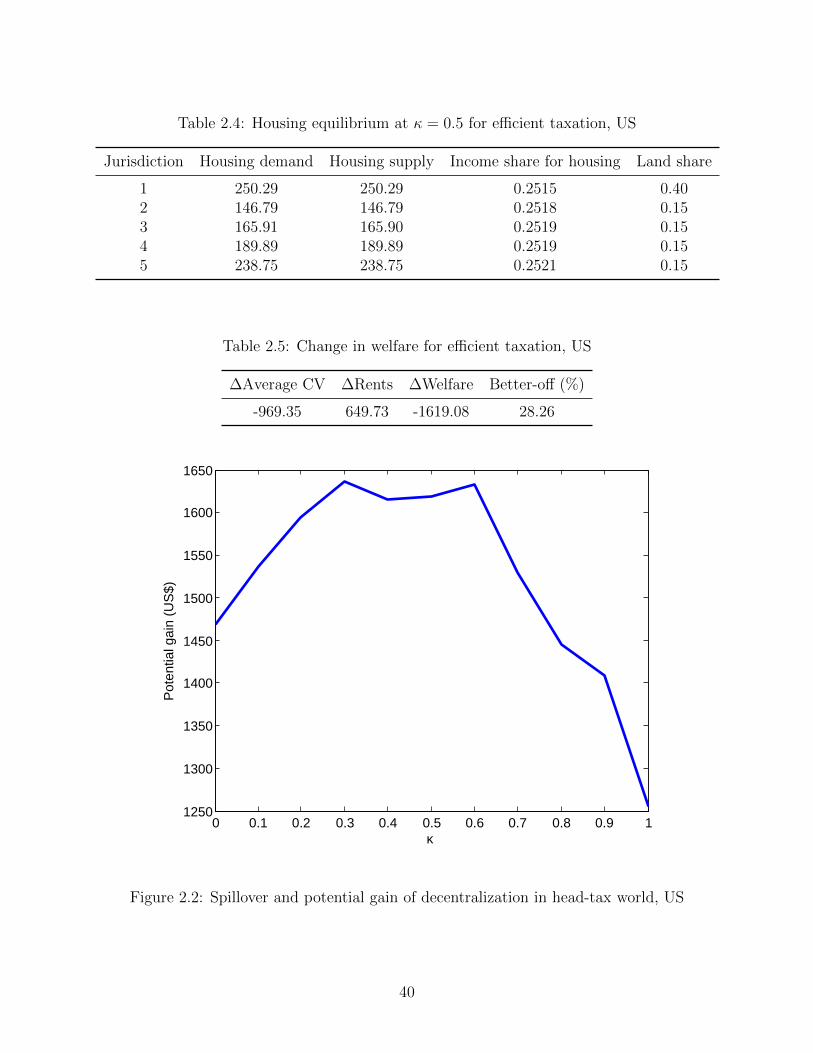
Table 2.4: Housing equilibrium at κ = 0.5 for efficient taxation, US

Jurisdiction Housing demand Housing supply Income share for housing Land share

1 250.29 250.29 0.2515 0.402 146.79 146.79 0.2518 0.153 165.91 165.90 0.2519 0.154 189.89 189.89 0.2519 0.155 238.75 238.75 0.2521 0.15

Table 2.5: Change in welfare for efficient taxation, US

∆Average CV ∆Rents ∆Welfare Better-off (%)

-969.35 649.73 -1619.08 28.26

0 0.1 0.2 0.3 0.4 0.5 0.6 0.7 0.8 0.9 11250

1300

1350

1400

1450

1500

1550

1600

1650Externality vs. Potential Gain, A Head−Tax Case (US)

κ

Pot

entia

l gai

n (U

S$)

Figure 2.2: Spillover and potential gain of decentralization in head-tax world, US

40

As we described previously, the main interest of this research is to observe how the

degree of spillover will impact the potential gain (of moving from centralized policy to decen-

tralized policy). Figure 2.2 exemplify the impact. The curve suggests that as the spillover

increases, generally the potential gain of decentralization decreases. This result support

Oates’ decentralization theorem (Oates, 1972): decentralization is favorable when spillover

among jurisdictions is relatively small. In our case, higher spillovers among jurisdictions

will impede the locals’ capability to set optimal tax rates. Figure 2.2 shows that when the

spillover is relatively low, the benefit from having positive spillovers (from other jurisdic-

tions) dominates the cost of having “non-optimal” public good provisions. However, as the

degree of spillover increases, the potential gain of decentralization declines.

Property taxation

In this section, we discuss the case where governments implements property taxation, as

opposed to efficient taxation. As before, we will examine the equilibrium, welfare change,

and a relationship between the spillover and the potential gain from the decentralization.

Table 2.6 shows that the housing price, local public good provision, and property

tax rate increase as we move from jurisdiction 1 (central city) to jurisdiction 5. The price

and local public good provision at the equilibrium are somewhat higher than those in the

efficient allocation case. The property tax rates in Table 2.6 are the percentage of annual

implicit rents that can be converted to property tax rates with a conversion rate 7-9 percent

(Poterba, 1992; Calabrese and Epple, 2010; Calabrese et al., 2012).

41

Table 2.6: Equilibrium at κ = 0.5 for property taxation, US

Jurisdiction Price Local public goods Property tax

1 14.33 1916.14 0.35592 16.24 3099.78 0.35983 17.21 3882.77 0.35694 18.42 5035.59 0.35455 20.82 8046.76 0.3566

In this property-tax setting, the distribution of population is more balanced than

that of the efficient allocation case. The central city has the largest population (approx.

40 percent) and the the rest of jurisdictions have fairly equal populations. It replicates the

results from Calabrese et al. (2012) when they are assuming there is no spillover in the

economy. It is also reported that jurisdictions have stratified mean income where the central

city has the lowest mean income (US$ 26,954) and jurisdiction 5 has the highest mean income

(US$113,310) in Table 2.7.

Table 2.7: Populations and mean incomes (property tax), US


1 0.39 26954.372 0.15 43692.873 0.15 54753.884 0.15 71008.765 0.16 113309.55

42

Table 2.8: Housing equilibrium at κ = 0.5 for property taxation, US


1 197.92 199.08 0.27 0.402 108.82 107.70 0.27 0.153 129.04 129.21 0.27 0.154 159.36 159.19 0.27 0.155 228.69 228.76 0.27 0.15

Table 2.9: Change in welfare for property taxation, US


195.32 -59.36 254.67 0

The housing market equilibrium is shown in Table 2.8. We have some discrepancies in

the housing equilibrium where housing demand is not exactly equal to the housing supply in

each jurisdiction. However, the the discrepancies are relatively very small. Income share for

housing is calculated approximately 0.27—which is a realistic number (Quigley and Raphael,

2004).

In this property-tax world society in total is worse-off when the regime is changed

into a decentralized taxation. Intuitively, when the degree of spillover is relatively high

(κ = 0.5), the negative impacts of non-optimal taxation and local public good provisions on

welfare dominate the benefits on enjoying positive externalities from other jurisdictions. As

the tax policy moves to decentralization, the average CV decreases by US$195.32 and the

rents decreases by US$59.36 (that will reduce landlord’s welfare level). Moreover, there is no

household will be better-off in this case. In aggregate the society is worse-off by US$254.67.

43

The potential cost of decentralization occurs in all level of spillover between 0 and 0.9

as shown in Figure 2.3.28 The trend of the graph in the property-tax case is unequivocal, as

opposed the corresponding figure in the efficient-taxation case. The graph demonstrates that

as the spillover increases, the potential loss of decentralization also increases. This result

firmly preserves Oates’ decentralization theorem (Oates, 1972).

0 0.1 0.2 0.3 0.4 0.5 0.6 0.7 0.8 0.9−600

−500

−400

−300

−200

−100

0Externality vs. Potential Gain, A Property Tax Case (US)

κ

Pot

entia

l gai

n (U

S$)

Figure 2.3: Spillover and potential gain of decentralization in property-tax world, US

28One of the limitations of the numerical simulation we used in this research is that it is very sensitive tothe choices of parameters and initial guess, where some combination of parameters and initial guess mightgenerate indefinite values or even complex numbers. For that reason, we can only have 0 ≤ κ ≤ 0.9 to depictthe impact of spillover on the potential gain of decentralization.

44

2.4.4 A case of an urban economy in Indonesia

2.4.4.1 Calibrations and results

In this section, we will discuss how some degree of spillover (κ = 0.5) will affect the equilib-

rium in housing market, local public good provision, and tax rates in a developing country.

We will also discuss the impact of spillover on welfare gain of decentralization in both head-

tax and property-tax worlds. We use Indonesia as representative of developing countries.

Indonesia is fairly new to fiscal and tax decentralization, especially for decentralized property

tax.29 We will also divide the discussion into two section: a case for head tax and a case for

property tax. Table 2.10 reports the parameters use for Indonesian case.

Table 2.10: Parameters, Indonesia

Parameters

number of communities 5µlny 9.8614σlny 0.8310βh 0.3959βx 1ρ -0.01γ 0.37θ 1.7κ 0 to 1

βh and γ are set to 0.37 and 0.3959 to get housing elasticity approximately 1.7 and

housing income share between 27% and 33%. Those values are based on the work of Monkko-

nen (2013) who studies housing markets in urban areas in Indonesia.

Efficient taxation

29Indonesia implemented fiscal decentralization in 2000 (Act no.22/1999) and decentralized property tax-ation in 2011 (Act no.28/2009).

45

Although head tax is not applicable in many places in the world, including Indonesia, we

use this type of tax as a benchmark when the tax does not generate distortion. A head tax

will not alter the household behavior and consequently will not create dead-weight loss in

the economy. A head tax is an efficient tax for that reason. We start with a head tax in this

section and then will be followed a discussion on the case of property tax in Indonesia.

The numerical simulation results in Table 2.11 shows that at κ = 0.5 housing price,

local public good provision, and head tax are stratified in five jurisdictions where the central

city has the lowest values and jurisdiction 5 has the highest values of those three variables.

The housing price in the central city is US$8.5 and the housing price in the jurisdiction 5 is

US$11.39. As expected, all corresponding values in equilibrium are lower than those in the

US case as the consequences of lower mean income. However, the distribution of population

in the metropolitan area is about fairly identical as reported in Table 2.12. The mean income

is only US$12,645.79 in the central city and US$102,237.52 in jurisdiction 5. Housing market

is in a equilibrium with income share for housing approximately 27 percent as shown in Table

2.13.

Table 2.11: Equilibrium at κ = 0.5 for efficient taxation, Indonesia

Jurisdiction Price Local public goods Head tax

1 8.85 809.59 809.592 9.96 1779.07 1779.073 10.33 2447.02 2447.024 10.82 3571.59 3571.595 11.39 6545.00 6545.00

46

Table 2.12: Populations and mean incomes (head tax), Indonesia


1 0.60 12645.792 0.14 27849.243 0.11 38244.284 0.09 55814.165 0.06 102237.52

Table 2.13: Housing equilibrium at κ = 0.5 for efficient taxation, Indonesia


1 230.89 230.89 0.27 0.402 107.82 107.82 0.27 0.153 115.46 115.46 0.27 0.154 125.73 125.73 0.27 0.155 138.31 138.31 0.27 0.15

Table 2.14: Change in welfare for efficient taxation, Indonesia


-419.2141 -1668.59 1249.37 30

The change in welfare as the regime move to a decentralized tax policy is reported

in Table 2.14. Although only 30 percent of households are better-off, the average CV has a

positive value meaning, on average, total households is better-off. However, since the rents

decreases by a larger value (i.e. landlords are worse-off), the total society (households and

landlords) is worse-off. In brief, at κ = 0.5, in the head-tax world, the decentralization policy

has negative impacts in the metropolitan area by US$1249.37. This result is different from

the result we have in the US, where in the head-tax world, decentralization policy potentially

provide more benefits to the metropolitan area.

47

Compare to the US case, the impact of spillover is smoother in this Indonesian case as

shown in Figure 2.4. As the curve shown, there is no significant impact on welfare gain when

the spillover level is relatively low (0 ≤ κ ≤ 0.3). At that range, there is an indication that

the costs of having non-optimal public-good provisions compensate the benefits from having

positive spillover of local public good. However, the higher kappa result in lower potential

gain of decentralization for the households. For instance, at κ = 1 decentralization will cost

the households approximately US$1430.86. In general, we can conclude that decentralized

tax policy potentially generates higher costs to social welfare in the urban area in Indonesia

and the cost is higher as the degree of spillover increases.

0 0.1 0.2 0.3 0.4 0.5 0.6 0.7 0.8 0.9 1−1450

−1400

−1350

−1300

−1250

−1200Spillover and Potential Gain, A Head Tax Case (MA in Indonesia)

κ

Pot

entia

l gai

n (U

S$)

Figure 2.4: Spillover and potential gain of decentralization in head-tax world, Indonesia

48

Property taxation

For the purpose of comparison, we intentionally use κ = 0.5 in Indonesian case where

the governments implement property tax. A detail worth mentioning is that the equilibrium

housing prices and property tax in this case have different patterns compared to our previous

results as shown in Table 2.15. Both prices and property tax rates satisfy housing market

condition as shown in Table 2.17. Intuitively, as the local public goods increases from juris-

diction 1 to jurisdiction 5, when households pay a high price, they have to be compensated

by a lower property tax rate, and vice versa. For instance, in jurisdiction 5 the housing

price (US$10.09) is lower than jurisdiction 2,3, or 4. Consequently, the property tax rate in

jurisdiction 5 is relatively high to finance a high provision of local public goods. Using the

same conversion as before, the actual property tax rates are in the range 0.4-0.9 percent,

which is close to the actual property tax rate in Indonesia.30

In this property-tax equilibrium, households are concentrated in the central city (61

percent) with mean income US$12,831 vis-a-vis only few households choose to live in juris-

diction 5 (2 percent) with mean income US$133,526.

Table 2.15: Equilibrium at κ = 0.5 for property taxation, Indonesia

Jurisdiction Price Local public goods Property tax

1 9.91 916.59 0.082 13.90 1579.07 0.083 11.50 2047.02 0.094 11.38 3571.59 0.095 10.09 6545.00 0.11

30Based on Act no.12/1994, property tax rate in Indonesia is 0.5 percent(http://www.tarif.depkeu.go.id/Bidang/?bid=pajak&cat=pbb).

49

Table 2.16: Populations and mean incomes (property tax), Indonesia


1 0.61 12830.812 0.23 32101.173 0.08 51520.814 0.05 76801.405 0.02 133525.54

Table 2.17: Housing equilibrium at κ = 0.5 for property taxation, Indonesia


1 231.67 231.98 0.29 0.402 156.29 156.70 0.29 0.153 111.31 111.06 0.29 0.154 109.08 109.09 0.29 0.155 86.096 86.032 0.29 0.15

Table 2.18: Change in welfare for property taxation, Indonesia


-1847.46 -1371.48 -475.985 100.00

50

0 0.1 0.2 0.3 0.4 0.5 0.6 0.7 0.8 0.9 1470

480

490

500

510

520

530

540

550

560

κ

Pot

entia

l gai

n (U

S$)

Figure 2.5: Spillover and potential gain of decentralization in property-tax world, Indonesia

In the property-tax world at κ = 0.5, the change in average CV is -US$1847 meaning

the average households are better-off. In contrast, landloards are worse-off since the rents

decline by US$1371. As a result, there is net potential gain from decentralized taxation as

much as US$476. In this specific setting all households enjoy the benefit of decentralization.

The impact of spillover level than can be concluded from Figure 2.5. The graph

demonstrates that as κ increases from 0 to 1, the potential gain from decentralization de-

creases. The graph demonstrates the same pattern as what we have in US case with opposite

sign of the potential gain from decentralization. However, the general conclusion remains

the same: decentralization is more favorable when there is no spillover or when spillover is

relatively low. Again, this result substantiates the idea of Oates’ decentralization theorem.

51

2.4.5 Summary

We evaluate the potential gains and costs of decentralized tax policy in urban economies

when the spillovers are present. Using degree of spillover equal to 0.5, we find that the

answer depends on the spillover level, income level, and type of taxation we have in the

urban economy. Using metropolitan areas in the United States as benchmark, in an efficient-

tax setting, decentralization will benefit the urban area with relatively high mean income

such as Boston metropolitan area in the United States. In contrast, the same setting will

generate costs to a metropolitan area that has a relatively low mean income (compared

to metropolitan area in the US), such as Jakarta, Indonesia. In the property-tax setting,

the results reverse. Decentralization benefits the urban economy when the mean income is

relatively low and generates costs to the urban economy when the mean income is relatively

high.

However, our focus is more on the impact of spillover on the welfare in lieu of the

magnitude of the potential benefits or costs. We find that for all cases, the potential benefits

decreases as the degree of spillover increases, albeit there is an anomaly in the efficient-tax

setting for low degrees of spillovers. From cost perspective, the potential cost of decentral-

ization increases as the degree of spillover increases. Simply put, we favor lower spillover

to gain more from decentralized tax policy. Our results resonate the Oates decentralization

theorem where decentralization is favorable when the spillover level is low.

52

2.5 Numerical Simulations: Income level, inequality, and welfare change

In this section, we discuss two main issues for robustness and further conclusions. First, how

different income level will affect the welfare gain from decentralization at different levels of

spillover. Second, how inequality will effect welfare gain from decentralization at different

levels of spillover.31

2.5.1 Income and welfare change

Figure 2.6 presents a relation between three vectors: the mean income in lognormal distri-

bution (µlny), spillover (κ), and the potential gain of decentralization.32 The 3-D surface

shows an indication that an economy with higher mean income will gain more benefit from

decentralized tax policy at various level of spillover level, ceteris paribus. Interestingly, when

the mean income is relatively low, a higher spillover level will decrease the benefit from de-

centralization. In contrast, when the mean income is relatively high, a higher spillover level

will increase the benefit from decentralization. Intuitively, holding the same standard devia-

tion of income, using a higher mean income in the model will generate wealthier households

in the same interval of income distribution that makes the proportion of the tax for each

household relatively lower. As a result, the cost of having non-optimal public good provision

is getting smaller while holding the benefit from enjoying the positive spillover constant.

31We use efficient tax to illustrate this case. Relatively small variation in parameter(s) might generatedisequilibria. The calibration shows that the property-tax model is more sensitive to the change of parameterssuch as mean income or standard deviation of income. See footnote 28.

32Using Heien (1968) where µy = exp(µlny+0.5σ2

lny) the actual range is approximately between US$35,000

and US$80,000.

53

0 0.2 0.4 0.6 0.8 1

10.4

10.5

10.6400

600

800

1000

1200

1400

1600

1800

2000

2200

2400

κµln y

Pot

entia

l Gai

n(U

S$)

(a)

0 0.2 0.4 0.6 0.8 1400

600

800

1000

1200

1400

1600

1800

2000

2200

2400

κ

Pot

entia

l Gai

n(U

S$)

µln y=10.4

µln y=10.5

µln y=10.6

(b)

Figure 2.6: Income level and welfare change at various degrees of spillover, US

54

2.5.2 Inequality and welfare change

To observe the impact of inequality on welfare gain of decentralization, we use standard

deviation of the the lognormal distribution as a proxy of inequality. In this case, a higher

the standard deviation σlny implies a higher inequality.33

Figure 2.7 demonstrates that as inequality increases, the potential gain of decentral-

ization is linearly higher. This pattern is consistent in different levels of spillover. However,

Figure 2.7 also shows that when the inequality is high, the impact of spillover level on the

benefit from decentralization become more inconclusive, at least visually.

33We calibrate the value of σlny by taking into account the discrepancy between inequality in US and In-donesia. However, it is worth noting that some development economists attempt to relate the Gini coefficientand lognormal distribution, e.g., Chotikapanich (1997) formulates a relation between the Gini coefficient andlognormal as G = 2Φ(

σlny√2

) − 1 where G is Gini coefficient and Φ is standard normal integral up to the

ordinateσlny√

2.

55

00.2

0.40.6

0.81

0.8

0.85

0.9500

1000

1500

2000

κσln y

Pot

entia

l Gai

n(U

S$)

(a)

0 0.2 0.4 0.6 0.8 1400

600

800

1000

1200

1400

1600

1800

κ

Pot

entia

l Gai

n(U

S$)

σln y=0.8

σln y=0.9

(b)

Figure 2.7: Inequality and welfare change at various degrees of spillover, US

56

2.5.3 A higher degree of spillovers and switching to centralization

Our previous results show that: as the degree of spillovers increases reasonably large, decen-

tralization will be less preferable—supporting Oates decentralization theorem (1972). As an

extension, the model also enables us to investigate the degree of spillovers, κ, that will turn

the decision on tax policy from decentralization to centralization by increasing the value of

κ until the potential benefit from decentralization is zero. The results will not change our

previous conclusions about how spillover will impact the potential benefit of decentraliza-

tion but they will provide information about the degree of spillovers when centralization is

more beneficial than decentralization in the context of countries at different points in the

development process.

Figure 2.8 and 2.9 show cases for the head-tax case in the United States and the

property-tax case in Indonesia.34 Figure 2.8 shows that, in the US head-tax case, as the

degree of spillovers higher than 1.6, centralized-tax policy will be more beneficial for the

society than decentralized tax policy. This means that centralized-tax policy is better than

decentralized-tax policy when the total benefit enjoyed by households from other jurisdictions

is 1.6 times higher than total benefit enjoyed by household in the corresponding jurisdiction.

Figure 2.9 provides information about Indonesian property-tax case where centralization

will be beneficial when the degree of spillovers is very high (κ > 6.8). This means that the

total benefit enjoyed by households from other jurisdiction is 6.8 times higher than the total

benefit enjoyed by households in the corresponding jurisdiction.

From policy perspective, the very high degree of spillovers necessary for the benefit

34Both the property-tax case in the United States and the head-tax case in Indonesia favor centralizationeven when κ = 0 (the potential gain of decentralization is already negative when κ = 0).

57

of decentralization to hit zero in both cases above implies that decentralization is better

than centralization for these cases since it is unlikely that spillovers would reach these levels.

Naturally, when the degree of spillover is high enough, for example larger than one, any

degree of rivalry and exclusiveness may induce the local government to set a price to limit

the number of consumers of the good. If instead, local public goods are non-rivalrous and

non-excludable, the policy option left for the government is centralizing taxation.

0 0.2 0.4 0.6 0.8 1 1.2 1.4 1.6−200

0

200

400

600

800

1000

1200

1400

1600

1800

κ

Pot

entia

l Gai

n(U

S$)

Figure 2.8: Potential gain from decentralization in the head-tax world, US

58

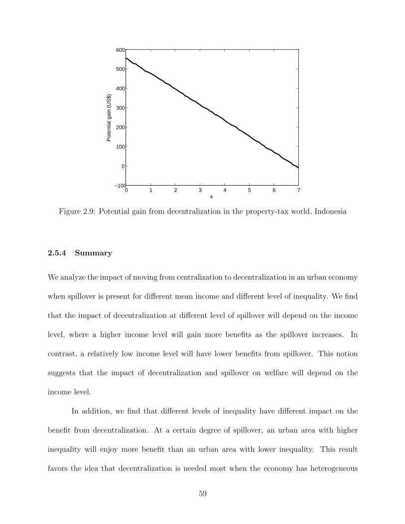
0 1 2 3 4 5 6 7−100

0

100

200

300

400

500

600

κ

Pot

entia

l gai

n (U

S$)

Figure 2.9: Potential gain from decentralization in the property-tax world, Indonesia

2.5.4 Summary

We analyze the impact of moving from centralization to decentralization in an urban economy

when spillover is present for different mean income and different level of inequality. We find

that the impact of decentralization at different level of spillover will depend on the income

level, where a higher income level will gain more benefits as the spillover increases. In

contrast, a relatively low income level will have lower benefits from spillover. This notion

suggests that the impact of decentralization and spillover on welfare will depend on the

income level.

In addition, we find that different levels of inequality have different impact on the

benefit from decentralization. At a certain degree of spillover, an urban area with higher

inequality will enjoy more benefit than an urban area with lower inequality. This result

favors the idea that decentralization is needed most when the economy has heterogeneous

59

population or jurisdictions.

Extending the degree of spillovers above the level of κ = 1 from the baseline spec-

ifications also provides us with intuition how high spillovers will switch the policy from

decentralization to centralization for the US head-tax case and the Indonesia property-tax

case. We find that the spillovers need to be very high (such that the benefit to those outside

the community exceeds that for those within the community) to be considered as a reason

to move from decentralization to centralization in both cases.

2.6 Conclusions and policy implications

This research has inquired a question about the impact of fiscal decentralization on welfare

both in developed and developing countries, especially in tax policy where spillovers of public

goods among jurisdictions are present. Two types of taxation are used in this research, i.e.

efficient tax and property tax. The theoretical framework of the model is built in Section

2.3 to support the construction of numerical simulation in Section 2.4. Estimations has been

made to gauge whether the benefits from fiscal decentralization (as in Tiebout equilibrium

literature) dominates the costs (as in the tax-competition literature). Moreover, as the main

contribution, this research takes into account the impact of spillover on the benefits of de-

centralization in the metropolitan area as discussed in Oates’ decentralization theorem.

The results from the numerical simulation shows that spillover level does affect the

potential gain of decentralization. Unexpectedly, in the case of efficient taxation, the impacts

of spillover are ambiguous. Relatively low level of spillover has a positive impact on the po-

tential gain of decentralization. In this case, the benefit from consuming local public goods

in different jurisdictions dominates the cost of having non-optimal tax rate and non-optimal

60

public good provision. However, as the degree of spillover increases, the potential gain of

decentralization diminishes in both cases of developed and developing countries. Moreover,

in the US head-tax case and Indonesia property-tax case, a very high degree of spillovers is

necessary to switch the policy from decentralization to centralization.

On the other hand, the impact of spillover level in property-tax case is unequivocal.

The numerical simulation shows that the spillover level does have negative impact on the

potential gain from decentralization. As the degree of spillover increases, the potential gain

of decentralization decreases in both developed and developing countries.

Overall, the results substantiate Oates’ decentralization theorem where decentraliza-

tion is more beneficial when spillovers among jurisdictions are relatively low. However, we

have to be aware that the impact of spillover level on the potential gain of decentralization

varies across different levels of income vis-a-vis income inequality. The result shows that a

metropolitan area with a relatively low mean income will be negatively affected by spillover,

and vice versa. The numerical simulation also shows that a higher level of inequality and in-

come amplify the benefits of decentralization. Although one might consider that this result

is politically incorrect, it illustrates that developed countries—that generally have higher

income inequality—potentially gain more benefits from decentralization.

From policy perspective, the results can provide some insights of decentralizing tax

policy. First, as a contrast to what we normally believe, the policy makers should be aware

that decentralization may generate loss to the society. It is very important that government

needs to be very careful in determining the type of taxation to decentralize. One important

factor is the level of spillover among jurisdictions, where a different level of spillover will have

different impacts on the welfare. This suggests that some taxes are better to remain under

61

centralized policy especially when the spillovers are very high as we discuss in Section 2.5.3.

A careful measure is important to define whether a certain tax should be decentralized or

centralized. Second, as the consequence of spillover, coordination among jurisdictions is very

important to minimize the negative impact of spillover in the metropolitan area. Consoli-

dating the resources and coordination in choosing the type and level of public good provision

are potentially beneficial to all jurisdictions in the metropolitan area and will minimize the

negative impact of spillover and potential costs of duplication.

At least there are four potentially appealing topics for future research related to this

discussion. First, a research question about how different type of taxation, such as income

tax, may have impact on the equilibrium and the social welfare. Second, a question about

the robustness of the model to different number of jurisdictions35 and the assumption of

land distribution, as well as the optimal number of jurisdictions in decentralized policy. This

question is relevant in developing countries that are new to decentralization, such as In-

donesia, where some jurisdictions have been proposing to have territorial reforms. Three,

whether that higher-income households enjoy more benefits from decentralized-tax policy as

indicated in Section 2.5 will be an intriguing topic for further research. It is interesting to

investigate whether, within community, higher-income households are better-off than lower-

income households as decentralized-tax policy is implemented by the government. Four,

taking into account administrative costs in implementing centralization versus decentraliza-

tion could be examined empirically and might provide additional insights.

35Calabrese et al. (2012) show that their model is robust to different assumptions regarding the numberof jurisdictions.

62

CHAPTER 3

Optimal Income-Sales Taxation, Tax Evasion, and Uncertainty

3.1 Introduction

3.1.1 Background

In the history of modern optimal tax theory from Ramsey (1927) on optimal commodity

taxation to Saez (2001) on using elasticity to derive optimal income taxation, not much

research incorporates tax evasion and uncertainty into optimal taxation models. Moreover,

most analysis focuses on indirect taxes alongside direct taxes rather than on finding the

optimal tax mix which is more practical politically in the real world (Boadway et al., 1994).

This is in line with a statement in Bradford and Rosen (1976),where there are two different

problems have been studied in the modern optimal tax theory: finding an optimal set of

commodity taxes and finding the optimal degree of income taxation.1

This research examines the optimal taxation in the presence of tax evasion and un-

certainty with focus on income-sales tax mix where the model is built based on Nava et al.

(1996), Boadway et al. (1994), and del Mar Racionero (2001). Similar to them, the model

utilizes a standard two-class economic model of optimal taxation where the government can-

not observe the agents’ ability but can observe income. Also, the government uses both

non-linear income and linear commodity taxes. By adopting Nava et al. (1996), we deal

with a two-class economy with two types of labor and two commodities and also taking into

account the existence of under-reported income (tax evasion) and uncertainty. Intuitively,

1Bradford and Rosen (1976) assumes that the revenue system is based on income rather than commoditytaxation.

63

by employing a balance budget constraint in the model, income tax will be higher as tax

evasion in the economy increases. In contrast to Cremer and Gahvari (1995), this paper in-

corporates the uncertainty of being detected from hiding some income to gain benefits from

lower tax payment, rather than the uncertainty of the wage. The cost function is adopted

from Boadway et al. (1994)2. We assume that the government implements balanced-budget

policy.

To answer the research questions, this research utilizes some standard assumptions

(see Section 3.3.1) and we only focus on certain variables in a system that we build as as

simple as possible. We believe this type of setting can provide intuitive results. Adding

more complexity will only generate a model with non-intuitive and mathematically complex

results and very likely only add small contributions to our understandings that are not the

main purpose of this research. Simply put, the main motivation of this research is to enrich

the existing model by adding more realistic variables with intuitive results. For instance, the

degrees of tax evasion in developed and developing countries are very likely to be different as

developed countries in general have better tax systems and institutions. It is expected that

the results can explain the real world and also contribute to the theory, at least by taking

into account uncertainty and tax evasion.

3.1.2 Research questions

Specifically we will answer four main research questions. Subject to a government revenue

constraint:

1. How will uncertainty affect the optimal income and sales tax rates?

2Boadway et al. (1994) defines the cost of hiding one dollar of income is G(1−σ), where σ is the proportionof reported income. G(.) is assumed strictly convex and non-negative.

64

2. How will tax evasion affect the optimal income and sales tax rate?

3. What factors will increase the optimal income and sales tax rate?

4. What factors will decrease the optimal income and sales tax rate?

3.1.3 Research outline

The essay is organized as follows. The following section will discuss literature review on

taxation that will cover common approaches in optimal taxation theory. The discussion will

be focused on the models, assumptions, results, and conclusions of the existing literature.

The section is then closed by a summary leading to the theoretical model in section 3.3.

Section 3.3 focuses on the process of building the model. It will be started by dis-

cussing the original model and follow by the discussion how the model will change when

we add tax evasion and uncertainty into the model. We put the details of the algebra in

the appendices. The final results in this chapter is the optimal income tax rates for both

high-type and low-type labors and also the optimal sales tax rates that directly comparable

to Nava et al. (1996) which do not have tax evasion and uncertainty in their model. Related

to our results, Nava et al. (1996) find that if a private good is a substitute for leisure, then

it is optimal to subsidize the high-type agent’s income at the margin (negative income tax).

The results in section 3.3 then will be discussed in section 3.4 along with the conclu-

sions and the policy implications of this research.

3.2 Literature Review

The standard framework for optimal taxation postulates that the tax system is designed

to maximize a social welfare function subject to specified constraints. The most common

65

constraint is that the government should meet a certain (or minimum) level of revenue. The

question is then what types of commodities should be taxed? How progressive or regressive

should the income tax be? Those normative questions have been the subject of key debate

by the most of prominent economists since Adam Smith up to today (Newbery and Stern,

1987).

For the purpose of this research, we will discuss the modern theories (utilitarian based)

that are characterized by welfare maximization problem that begins in 1927 by Frank Ram-

sey.3 Modern theory of public economics utilizes the fundamental theorems of economics:

(1) competitive equilibrium is Pareto efficient and (2) a Pareto-efficient outcomes can be

achieved as competitive equilibrium if prices are set appropriately and lump-sum incomes

are allocated so that each individual can buy the consumption bundle given in the allocation

at the prices that will prevail (Newbery and Stern, 1987). This section will discuss related

literature review that provide underpinnings to the theoretical framework to construct the

model and to support the analysis.4

3.2.1 Commodity taxation

Ramsey (1927) shows that to reach maximum welfare that meet required government rev-

enue from commodity taxes, the proportional change in demand should be the same for all

3In the nineteenth century, the discussion was focused on conceptual framework such us ability to payand tax base (Newbery and Stern, 1987). We may also find non-welfarist approaches to optimal taxationsuch as behavioral economic approach (see Kanbur et al., 2006) and macroeconomic or economic growthapproach (see Barro and Sala-i Martin, 1992).

4Another factor such as institutions is not discussed in this research. Readers who are interested in thisarea may refer to Slemrod (1990) and Alm (1996).

66

commodities that give us the following famous result:

∑i

TiSik = bxk, k = 1, ...,m (3.1)

where Ti is per unit tax of good i, xk is the quantity of good k, Sik is the elasticity for good

i with respect to the price of good k and b is some constant.

In the elasticity term then we have a familiar result known as inverse elasticity rule

as follows:

tr =d

εrr(3.2)

where tr is the tax rate (= Tr/Pr), d is a constant, and εrr is the elasticity of uncompensated

demand for good k. This result has an intuitive interpretation: the imposition of a tax

on an inelastic good will have smaller effects on consumer behavior than that on elastic

good, which consequently result in smaller deadweight loss. Equity is not an issue here since

Ramsey assumes all individuals are identical.

3.2.2 Income taxation

Another important work on optimal tax policy is from Mirrlees (1971). Contrast to Ram-

sey, Mirrlees (1971) formalizes a social planner’s problem with unobserved heterogeneity of

individuals. In his paper, Mirrlees (1971) assumes both log normal and Pareto distribution

of earning abilities and focuses on nonlinear income taxation. The question is about how

to obtain an income tax schedule (tax function) that maximizes the social welfare function

67

(sum of all individuals’ utilities in the economy) subject to the revenue constraint. Mirrlees

assumes that the utility function is in the form of a Cobb-Douglas utility function and the

main result of his model are: (1) the marginal tax rate should be between zero and one; (2)

the marginal tax rate for the person with the highest earnings should be zero; and (3) if the

person with the lowest wage is working at the optimum, then the marginal tax rate that the

person faces should be zero. Using a marginal tax rate, tax payers are classified into tax

brackets, which determine which rate taxable income is taxed at. As income increases, it

will be taxed at a higher rate than the first dollar earned.

Other than its complexity, one of Mirrlees results’ weaknesses is the unweighted sum

of individual utilities (Bradford and Rosen, 1976). This implies that the marginal contribu-

tion of a rich individual to the social welfare function is the same as a poor one. Moreover,

Saez (2001) points out the limitation of Mirrlees’ approach in application for three reasons:

(1) the zero marginal rate at the top of income is a very local result; (2) based on his nu-

merical simulations, the tax schedules are easily affected by the form of the utility function;

and (3) the Mirrlees’ result does not change the way the public economists think in practice

about the efficiency-equity trade-off where the discussion still focuses on the efficiency side

rather than the equity side. To have more applicable result, Saez (2001) using elasticities

to derive the optimal income tax rates. By utilizing the elasticities, he is able to performed

a numerical simulation using empirical income distributions. His simulation results suggest

that the marginal tax rates labor income should be between 50%-80%.

68

3.2.3 Direct-indirect taxation

We now turn to direct-indirect taxation that will be discussed mostly based on the work of

Atkinson and Stiglitz. Using one representative consumer facing a set of commodity taxes,

Atkinson and Stiglitz (1972) illustrates that if goods and leisure are separable, the optimal

commodity tax structure is uniform (or the optimal structure is identical to a proportional

income tax). They also show that when the utility function is separable between labor and

all commodities, no indirect taxes are needed. Consequently, the Ramsey result is only

relevant where there are constraints to implement income taxation (Atkinson and Stiglitz,

1976). Another important theoretical result from Atkinson and Stiglitz is: if the government

only focuses on efficiency, it may use only direct taxation and it would take the form of a

poll tax

However, the result in Atkinson and Stiglitz (1972, 1976) no longer holds if the model

includes the production side of the economy (Naito, 1999). In his paper, he shows that if the

nonlinear income tax system is implemented for redistribution purpose, the introduction of

distortions in the public sector can be a Pareto improvement (in contrast to Diamond and

Mirrlees, 1971).5

5In other word, the public sector is not necessarily efficient. The intuition is that by hiring more unskilledworkers, the government will generate less unskilled workers in the private sector and indirectly redistributeincome from skilled to unskilled workers (Naito,1999).

69

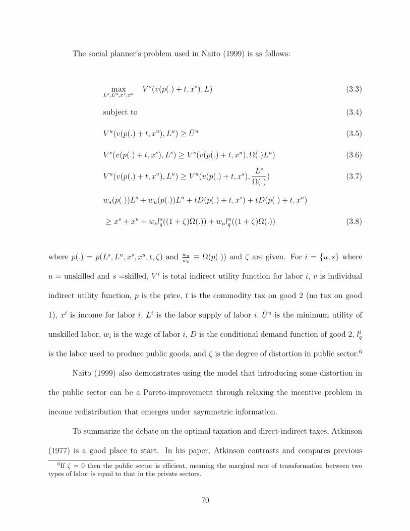
The social planner’s problem used in Naito (1999) is as follows:

maxLs,Lu,xs,xu

V s(v(p(.) + t, xs), L) (3.3)

subject to (3.4)

V u(v(p(.) + t, xu), Lu) ≥ Uu (3.5)

V s(v(p(.) + t, xs), Ls) ≥ V s(v(p(.) + t, xu),Ω(.)Lu) (3.6)

V u(v(p(.) + t, xu), Lu) ≥ V u(v(p(.) + t, xs),Ls

Ω(.)) (3.7)

ws(p(.))Ls + wu(p(.))L

u + tD(p(.) + t, xs) + tD(p(.) + t, xu)

≥ xs + xu + wslsq((1 + ζ)Ω(.)) + wul

uq ((1 + ζ)Ω(.)) (3.8)

where p(.) = p(Ls, Lu, xs, xu, t, ζ) and wuws≡ Ω(p(.)) and ζ are given. For i = u, s where

u = unskilled and s =skilled, V i is total indirect utility function for labor i, v is individual

indirect utility function, p is the price, t is the commodity tax on good 2 (no tax on good

1), xi is income for labor i, Li is the labor supply of labor i, Uu is the minimum utility of

unskilled labor, wi is the wage of labor i, D is the conditional demand function of good 2, liq

is the labor used to produce public goods, and ζ is the degree of distortion in public sector.6

Naito (1999) also demonstrates using the model that introducing some distortion in

the public sector can be a Pareto-improvement through relaxing the incentive problem in

income redistribution that emerges under asymmetric information.

To summarize the debate on the optimal taxation and direct-indirect taxes, Atkinson

(1977) is a good place to start. In his paper, Atkinson contrasts and compares previous

6If ζ = 0 then the public sector is efficient, meaning the marginal rate of transformation between twotypes of labor is equal to that in the private sectors.

70

research on optimal taxation (both direct and indirect taxation) by comparing two main

views: (1) desirable balance which appears to find favors with policy makers where direct

taxation is used for equity purpose while indirect taxation is used for efficiency purposes;

and (2) direct taxation is superior on both equity and efficiency purposes.

Comparing four models from previous research, Atkinson summarizes that if all con-

sumers are identical then the poll tax is efficient. However, if the consumers are not iden-

tical (by varying wages) the optimal tax depends on goods consumed which will depend on

marginal value of income. By considering distribution, redistribution with indirect taxes

supports heavier taxes on luxury goods, albeit this is not always the case where he shows

that in linear expenditure system the optimum indirect tax would be the same tax rates

for all commodities. Intuitively, the progressiveness of commodity tax exactly offsets the

regressiveness of the lump-sum tax.

Stiglitz (1982) works on the Pareto efficient taxation by assuming two-class econ-

omy (high and low abilities) and incorporating self-selection constraints—also known as the

incentive compatibility constraints—in the planner’s maximization problem. The formal

71

representation of the model is as follows:

maxC1,C2,Y1,Y2

V 2(C2, Y 2) (3.9)

subject to: (3.10)

V 1(C1, Y 1) ≥ U1 (3.11)

V 2(C2, Y2) ≥ V 2(C1, Y1) (3.12)

V 1(C1, Y1) ≥ V 1(C2, Y2) (3.13)

R = (Y1 − C1)N1 + (Y2 − C2)N2 ≥ R (3.14)

where Ci and Yi are the i-th individual’s consumption and income, respectively. V i is i-th

individual’s indirect utility, Ni is the number of individuals of type i, R is government rev-

enue, R is the revenue requirement. The result for this planner’s problem will depend on

the assumption on whether the self-selection constraint is binding or not. In the normal case

where the self-selection constraint for high type is binding and the self-selection constraint

for low type is not binding, he found that the marginal tax rate for the low type is positive

and the marginal tax rate for the high type is zero as demonstrated in Mirrlees (1971).

In the existences of both income and commodity taxation, by modifying the govern-

ment budget constraint, Stiglitz (1982) concludes that if the leisure and goods are separable,

there should be no commodity taxation (only a income tax is needed). This notion supports

the result in Atkinson and Stiglitz (1976) as we discussed previously. The intuition is that

with the separability, if those two types have the same indifference curve between two com-

modities, one cannot use differential taxation as a basis of separation.

72

Boadway et al. (1994) argues that in any case the existing theory does not tell any-

thing about the mix of direct and indirect taxes. He points out that the existing theory

only has two type of results when the government wants to impose both direct and indirect

taxes: (1) income taxation is enough or (2) the tax mix is indeterminate since the optimal

tax structure can be achieved by an arbitrary combination of direct-indirect taxation. In

order to capture this issue, Boadway et al. (1994) uses an analysis based on the concept

that different taxes will have different tax evasion features where the incentive to evade will

depend on the marginal tax rates. In the world of two types of individuals, two consumption

goods, a direct-indirect tax mix, and the possibility of hiding some proportion of income

along with the concealment costs, Boadway et al. (1994) shows that in the existence of tax

evasion the incompatibility constraint play an important rule in the design of tax system.

This notion bring us to the model that we will construct in Section 3.3.

As far as this research is concerned, Nava et al. (1996) shows that the good comple-

mentary with leisure should be taxed higher. It is also implicitly assumed in their paper

that all households’ income are fully reported which is not always true in the real world.

It brings us to the notion that including the possibility of tax evasion along with its cost

will change the results and provide a more realistic model. Unlike them, we do not focus on

public expenditure policy.7 We simply focus on the optimal taxation for both income and

sales taxes.

7To deal with public expenditure policy, Nava et al. (1996) modify the standard Samuelson rule by addingterms related to the self-selection constraint and to the revenue of indirect taxes.

73

3.2.4 Summary

The literature review section discusses some modern approaches that has been used to define

an optimal taxation theory. From the inverse elasticity rule from Ramsey (1927) to using

elasticity to derive optimal income taxation from Saez (2001), there are various approaches

that provide a broad range of understanding on optimal taxation.

The optimal taxation theory focuses on three cases: (1) linear commodity taxation

as we see in Ramsey (1927); (2) non-linear income tax as in Mirrlees (1971); and (3) direct-

indirect taxes as in Atkinson and Stiglitz (1976) and Stiglitz (1982). It is the direct-indirect

taxation that becomes main interest in this research. Many papers have been written based

on Atkinson and Stiglitz (1976), including Nava et al. (1996) and Boadway et al. (1994).

The optimal balance of direct and indirect taxation maybe is the most practical

question in real world. The optimal taxation theory has provided such useful insights eco-

nomically based on utilitarian paradigm. However, not all are acceptable politically. The

notions of uniform indirect taxation and only having income taxation in the economy only

make sense to economists but not for policy makers or average voters.

As expected, all type of economic models may need to include some conceptions that

usually ignored in the model. The discussion on the best model is always debatable since

every model will have its unique insights in its specific settings. As in Mankiw et al. (2009),

how to take into account new ideas into the theory of optimal taxation remains an open

question.

74

Using the model developed by Nava et al. (1996), this research tries to provide new

insights to the existing model, i.e. a model that can provide a new guidance on how the

government should define the optimal income and sales tax rates.

3.3 The Model

In this section, we will discuss the assumptions used in the model, the household’s maxi-

mization problem, the mimicker’s maximization problem, and the social planner’s problem.

We will discuss the main results and leave the details of algebra in the appendices.

3.3.1 Assumptions

As in standard literature, we assume there are two types of households in the economy: low

type and high type. The government is not able to observe the ability of the individuals (or

households) but can observe the individual’s income. However, the individuals are able to

conceal their income and concealing is a costly behavior where the cost is linear. Government

imposes an income tax rate (ti) where i refers to household i.

Both high type and low type pay tax and only possible to conceal income, not expen-

diture. It means there is no uncertainty in sales tax. There are two types of consumption

goods (private goods): good a (xa) and good b (xb) where government only imposes sales tax

on good a (τa)and leave good b untaxed (τb = 0) therefore good b is treated as a numeraire.

In this setting, we assume that the income taxes are non-linear and commodity taxes are

linear.

The final objective of the model—as well as the main objective of this research—is to

solve a social planner’s problem. However, to achieve it, we need to solve for the household’s

75

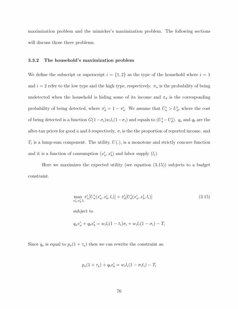
maximization problem and the mimicker’s maximization problem. The following sections

will discuss those three problems.

3.3.2 The household’s maximization problem

We define the subscript or superscript i = 1, 2 as the type of the household where i = 1

and i = 2 refer to the low type and the high type, respectively. πu is the probability of being

undetected when the household is hiding some of its income and πd is the corresponding

probability of being detected, where πid = 1− πiu. We assume that U iu > U i

d, where the cost

of being detected is a function G(1−σi)wili(1−σi) and equals to (U iu−U i

d). qa and qb are the

after-tax prices for good a and b respectively, σi is the the proportion of reported income, and

Ti is a lump-sum component. The utility, U(.), is a monotone and strictly concave function

and it is a function of consumption (xia, xib) and labor supply (li).

Here we maximizes the expected utility (see equation (3.15)) subjects to a budget

constraint.

maxxia,x

ib,liπiu[U

iu(x

ia, x

ib, li)] + πid[U

id(x

ia, x

ib, li)] (3.15)

subject to

qaxia + qbx

ib = wili(1− ti)σi + wili(1− σi)− Ti

Since qa is equal to pa(1 + τa) then we can rewrite the constraint as:

pa(1 + τa) + qbxib = wili(1− σiti)− Ti

76

Define g(1− σi) ≡ G(1− σi)(1− σi), we have the maximization problem as follows:

maxxia,x

ib,liU iu(.)− πidg(1− σi)wili s.t. pa(1 + τa)x

ia + qbx

ib = wili(1− tiσi)− Ti (3.16)

By Roy’s identity we obtain:

V iτa =

dU

dτa=∂L∂τa

∣∣∣∣∗

= −αixia (3.17)

V iti

=dU

dti=∂L∂ti

∣∣∣∣∗

= −αiwiliσi (3.18)

V iTi

=dU

dTi=∂L∂Ti

∣∣∣∣∗

= −αi (3.19)

V iσi

=dU

dσi=∂L∂σi

∣∣∣∣∗

= −wili(πidg′(1− σi) + αiti) (3.20)

where αi is the marginal utility of income.

3.3.3 The mimicker’s maximization problem

Now, let us investigate the maximization problem faced by a mimicker. A mimicker—denoted

by a horizontal bar above the variables—is a high-type individual that imitate the behavior

of a low-type individual.

Define that l2 ≡ w1l1w2

, σ2 ≡ σiwiliw2 l2

, x2a(τa, t1, T1; l2, σ2), x2

b(τa, t1, T1; l2, σ2), V 2(τa, t1, T1) ≡

U2(x2a(.), x

2b(.),

w1l1(.)w2

; σ2), then the maximization problem for a mimicker is as follows:

maxx2a,x

2b ,l2U(x2

a, x2b , l2)− π2

dg(1− σ2)w2l2 s.t. w2l2(1− t1σ2)− T1 − x2a(1 + τa)− x2

b (3.21)

77

resulting:

V 2τa = −α2x

2a + α2∂w1l1

∂τaξ (3.22)

V 2t1

= −α2w1l1σ2 + α2∂w1l1∂t1

ξ (3.23)

V 2T1

= −α2 + α2∂w1l1∂T1

ξ (3.24)

V 2τ2

= −w1l1(α2t1 + π2dg′(1− τ2)) (3.25)

where8

ξ ≡Ul2w2α2

+ (1− t1σ2)− π2dg(1− σ2)

α2

3.3.4 The social planner’s problem

Now we turn to the social planner’s problem. The planner chooses a set of τa, ti, Ti that

will maximizes the utility of the high-type individual V 2(.) (see equation (3.26)) whilst in the

same time it guarantees that the low type will have at least a certain level of utility, U1s , as it

is shown in the first constraint. The second constraint is an incompatibility constraint or a

self-selection constraint that make sure that the high-type individual does not masquerade as

a low-type individual. Since the government guarantee that the low type will reach a certain

level of utility, the low type will not try to mimic the high type.9 The third constraint is the

government’s budget constraint where n1 and n2 are the number of low-type and high-type

individuals, respectively.

8If the individual reports all of her income, σ2 = 1, we have ξ as in Nava et al. (1996).9This is known as the normal case in Stiglitz (1982).

78

The left-hand side of the inequality is the total government revenue and,—as it is

shown in the third constraint—, it must be higher than or at least equal to some level of

revenues, R0. The social planner’s problem is then constructed as follows:

maxτa,ti,Ti

V 2(τa, t2, T2) (3.26)

subject to:

MUC : V 1(τa, t1, T1) ≥ U1s

ICH : V 2(τa, t2, T2) ≥ V 2(τa, t1, T1;w1l1(.)

w2

)

GBC : n1[τax1a(.) + σ1t1w1l1(.) + T1] + n2[τax

2a(.) + σ2t2w2l2(.) + T2] ≥ R0,

where MUC is the the minimum utility constraint for the low type, ICH is the incentive

compatibility constraint for the high-type, and GBC is the government budget constraint.

By utilizing the results from previous section (see the appendices for details), we are able to

derive an optimal income and sales taxes as follows:10

t1 =∂x1

a/∂t1

−∂w1l1/∂t1

τaσ1

+γα2

λn1σ1

ξ (3.27)

t2 =∂x2

a/∂t2

−∂w2l2/∂t2.τaσ2

(3.28)

τa =γ

λα2(x1

a − x2a)

[n1∂x1

a

∂τa

∣∣∣∣l1

+ n2∂x2

a

∂τa

∣∣∣∣l2

]−1

, (3.29)

10µ and λ are positive due to the monotonicity of preferences, and γ is strictly positive when U1s is

sufficiently high as shown in Nava et al. (1996). We also assume that the result is not a corner solution asprivate good can increase to infinity and leisure is capped at 24 hours per day.

79

where xia and li denotes the compensated demand for xa and compensated labor supply, re-

spectively.

We begin the analysis from the tax rate for the high-type, t2. Without losing the gen-

erality, we assume that τa > 0 regardless its optimality. Intuitively, we have the denominator

−∂w2l2/∂t2 > 0: the higher the income tax rate, the lower the labor supply and consequently

the income w2l2 (note that we have a negative sign in the denominator). We also have the

ratio τaσ2

is positive. Therefore, the sign of t2 will depend on the sign of ∂x2a/∂t2. Moreover,

t2 is non zero even at the top of income distribution since there is inefficiency generated by

the sales taxes. A distortionary income tax is still needed to compensate the inefficiency

(Nava et al., 1996).11

The sign of ∂x2a/∂t2 depends on the the propinquity between good a and leisure. If

good a and leisure are substitutes in the Hicks perception, then ∂x2a/∂t2 < 0 and t2 < 0. It

implies that it will be optimal if we subsidize the high-type individuals. In contrast, if good

a and leisure are complementary, then ∂x2a/∂t2 > 0 and consequently t2 > 0.

Equation (3.28) also demonstrates an intuitive result that the income tax rate is

inversely related to the proportion of reported income, σ2. The higher the degree of tax

evasion (i.e. the lower reported income), the higher the income tax rate. Specifically, this

result aligns with Nava et al. (1996) as it is assumed implicitly that σ2 = 1. Assuming

that good a and leisure are complementary and τa > 0, it is easy to see that t2 > τa if the

elasticity of demand for good a with respect to the high-type income tax is higher than the

elasticity of labor supply with respect to the high-type income tax, and vice versa.

11Nava et al. (1996) points out this in the context of comparing his results to that of Stiglitz (1982)where no marginal income tax on high-type individuals is needed when both direct and indirect taxes arenon-linear.

80

These results then come to four proportions:

Proposition 1. In a Pareto optimum, the income tax of the high-type individual will benegative (t2 < 0) if good a is a substitute for leisure.

Proposition 2. In a Pareto optimum, the income tax of the high-type individual will bepositive (t2 > 0) if good a is a complement for leisure.

Proposition 3. In a Pareto optimum where tax evasion exists, the income tax rate forthe high-type individual will be higher as the degree of tax evasion increases.

Proposition 4. In a Pareto optimum where good a and leisure are complementary,t2 > τa if the elasticity of demand for good a w.r.t. the high-type income tax is largerthan the elasticity of labor supply w.r.t. the high-type income tax.

Now we turn to the result in equation (3.27). To make it comparable directly with

the corresponding result in Nava et al. (1996), we will modify equation (3.27). Defining

ξ ≡ Ul2w2α2

+ (1− t1σ2), then:

t1 =∂x1

a/∂t1

−∂w1l1/∂t1

τaσ1

+γα2

λn1σ1

[ξ − π2

dg(1− σ2)

α2

](3.30)

One can observe that ξ is equal to ξ defined in Nava et al. (1996) when σ2 = 1, and

consequently equation (3.30) aligns with the result for t1 in Nava et al. (1996) when σi = 1

and the probability of being detected for high-type, π2d, is zero.12 Both results are also

identical when σ1 = 1 and the cost of hiding the income, g(.) is zero.13 In essence, the case

in Nava et al. (1996) is a special case of our analysis. It is interesting to see that in this

setting the income tax rate for the low-type individual is also affected by the probability of

being detected for the high type.

Assuming that the first term in (3.30) is positive as for t2, then it is intuitive that t1

will decrease as the probability of being detected for the high type increase, ceteris paribus.

12In this case ξ > 0 as it has been proved in Nava et al. (1996).13It is naturally assumed that g(0) = 0.

81

A higher π2d implies higher government revenues and accordingly lower the income tax rate

of the low type in this case.

The analysis of the effects of the first term in the right-hand side on t1 is analog

to the previous discussion on t2. The second term provide more information about the

optimal income tax rate for the low type where the tax rate will be positively affected by

γ, α2 and will be negatively affected by λ, n1, σ1, π2d, g(.). These results then provide two

propositions:

Proposition 5. In a Pareto optimum, the income tax of the low-type individual willdecrease as the probability of being detected for the high type increase, ceteris paribus .

Proposition 6. In a Pareto optimum, the optimal income tax rate for the low type willbe positively affected by γ, α2 and will be negatively affected by λ, n1, σ1, π

2d, g(.)

3.4 Conclusions and policy implications

In this research we have introduced uncertainty and tax evasion into an optimal tax mix

problem in two-class economy with two consumption goods and labor. We assume that the

government cannot observe the agent’s ability and only able to observe unconcealed income,

where concealing is a costly behavior for the agent. We also assume that the income taxes

are non-linear and the commodity taxes are linear. The model has beed constructed based

on the approach used by Boadway et al. (1994), Nava et al. (1996) and del Mar Racionero

(2001).

After taking into account uncertainty and tax evasion, as in Nava et al. (1996) we

also find that in the Pareto optimum the sign of income tax for the high-type agent depends

on the relation between the (taxed) private good and leisure. If the private good is a sub-

stitute for leisure, then the income tax for the high-type will be negative. However, if the

private good is a complement for leisure, the income tax of the high type will be positive.

82

As far as the tax evasion is concerned, the income tax for the high-type individual will be

higher as the degree of tax evasion increases. Intuitively, this result is the consequences of

the government’s budget constraint: to maintain the balanced budget, income tax should be

high when tax evasion is high. We also find that if the taxed private good and leisure are

complementary—i.e. when the income tax is positive for the high type—and the elasticity of

demand with respect to income tax is larger than the elasticity of labor supply with respect

to income tax, the commodity tax rate is higher than the income tax rate.

For the case of low-type, the model shows that the income tax of the low-type in-

dividual decreases as the probability of being detected for the high-type increases, ceteris

paribus. The result shows that the optimal income tax rate for the low-type individual in-

creases as the marginal utility of mimicking the low type or the marginal utility of income

for the mimicker increases, ceteris paribus. In other words, income tax for the low-type will

increase if the high type has more incentive to mimic the low-type. Conversely, the optimal

income tax decreases as the marginal utility of tax revenue, the number of low-type agents,

proportion of reported income, probability that the high-type will be detected when hiding

the income, or the cost of hiding the income increases.

In spite of the fact that the model is abstract, it has policy relevance. First, as shown

above, income tax is not necessary higher for the high type (high income), or even negative to

increase the total welfare. Although it might not sound politically correct, our result shows

that it will depend on the agent’s behavior toward leisure. Second, in order to reduce the

income tax rate for the low type, the policy maker needs to build a reliable tax system that

can reduce the possibility of tax evasion and consequently will increase the tax collection

rate.

83

As policy makers and most economists believe that the income tax can be utilized

as a tool to increase equality, there is a trade-off between equality and efficiency. A higher

income tax rate for the high types may reduce inequality and in the same time it will also

reduce efficiency as there will be less incentive for the high type to work more. One can argue

that it depends on the labor supply elasticities of low and high types as their after-tax wages

changes. As in Hausman (1983) and Nava et al. (1996), our results show that, by taking

into account the level of tax evasion, the higher elasticity will result in a lower tax rate to

maintain an optimum welfare level. Regarding equity, if the high type more responsive to

the income tax rate, the income tax rate should be less progressive and equity will be more

difficult to achieve. An optimum policy to deal with the trade-off remains an open question

that will be an interesting for a further empirical research topic. Institutional factors, such as

tax and political systems, would be important to be considered in theoretical and empirical

research.

Taking into account tax evasion in the model is crucial since the case will be con-

siderably different for developed and developing countries. Developed countries, in general,

have better tax systems than developing countries do; and consequently the degrees of tax

evasions will be different. Our model captures this notion. As the optimal income and sales

tax rates will be higher for a higher degree of tax evasion, we can expect that developing

countries will need to impose higher tax rates to meet some level of tax revenue, ceteris

paribus. One way to reduce the tax rates—that will be beneficial for poor households via a

lower income tax rate—is by implementing a more reliable tax system to reduce tax evasion.

Further research on different impacts of tax evasions in developed and developing countries

is warranted.

84

CHAPTER 4

Concluding Remarks

This dissertation examines two topics in economics. First, the impacts of spillovers

of public goods on the potential benefits from decentralized policy in urban economy. Do

spillovers of local public goods across jurisdictions have impacts on the potential gain of

decentralization in an urban economy? Are the impacts different for urban economies in

developed and developing countries? Those two questions are the main research questions

that we investigate in the first topic. Second, the role of tax evasion and uncertainty on

the optimal taxation. Specifically, how tax evasion and uncertainty will affect the optimal

taxation for both income and sales taxes in a two-class economy.

In investigating the first topic in Chapter 2, it is impossible not to mention Oates’

fiscal decentralization theorem (Oates, 1972) that shed light on the formal economic intuition

on centralization versus decentralization. Oates (1972) points out that decentralization will

be optimal if there is no spillover. Specifically, decentralized local public good provisions

based on local preferences will generate a higher social welfare than centralized local public

good provision with uniform levels of public good for all jurisdictions. Enhancing the simu-

lation model used by Calabrese et al. (2012), this dissertation illustrate the direction of the

impact of spillover on the potential benefits from decentralization. The findings in Chapter

2 support the idea of Oates decentralization theorem whereas the degree of the spillover is

sufficiently high, the potential benefit from having decentralization decreases. The results

are consistent in both urban economies in developed and developing countries.

85

From policy perspective there are two potential questions in two different situations

that might arise. First question: do we need to decentralize the tax policy? The answer

will then depend on the levels of spillovers across a jurisdictions. An appropriate method

to measure the spillover level will be another challenging task that is needed to be carefully

approached. One may expect that the task will not be simple since it will involve agents’

behaviors and preferences that are always difficult, if not impossible, to reveal. Second

question: assuming the decentralized tax policy has been implemented, how can governments

formulate a certain policy that can limit spillovers? In practice—regardless its advantages

and disadvantages—the implementation of school neighborhood zoning policy or other zoning

regulations is one possible answer. However, it might not be easy to find answers for another

type of local public local goods, such as recreation areas or other kinds of city public amenities

due to their characteristics as public goods which are non-rivalrous and non-excludable at

certain levels.

The second topic is discussed in Chapter 3 where the model is built based on Nava

et al. (1996) and Boadway et al. (1994). As in Nava et al. (1996), the results show that the

sign of the income tax for the high type will depend on the behavior of the high type toward

leisure. If the (taxed) consumption good is a complement for leisure then the income tax

rate will be positive. In contrary, if the consumption good is a substitute for leisure then the

optimal income tax will be negative. By taking into account tax evasion and uncertainty, the

findings shows us that higher tax evasion will increase the income tax rates. In addition, the

income tax rates for the low type will increase if the high type has more incentive to mimic

the low-type and the probability of getting caught (when hiding some portion of income) is

low.

86

From policy perspective, when the high type is mimicking the low type, the effec-

tiveness of income tax as a redistribution tool will be lower. Lower tax evasion and higher

tax compliance will lower the income tax rate for the low-type and consequently increase

the equity. The importance of a reliable tax system and simple tax codes are imperative to

reduce the potency of tax evasion. This is relevant for economies globally where degree of

tax evasion may vary as tax systems and institutions in general are different.

87

BIBLIOGRAPHY

Akai, N. and Sakata, M. (2002). Fiscal Decentralization Contributes to Economic Growth:Evidence from state-level cross-section data for the United States. Journal of UrbanEconomics, 52(1):93–108.

Alesina, A. and Spolaore, E. (1997). On the Number and Size of Nations. The QuarterlyJournal of Economics, 112(4):1027–56.

Alm, J. (1996). What is an Optimal Tax System. National Tax Journal, 49(1):117–133.

Arnott, R. J. and Stiglitz, J. E. (1979). Aggregate Land Rents, Expenditure on PublicGoods, and Optimal City Size. The Quarterly Journal of Economics, 93(4):471–500.

Atkinson, A. B. (1977). Optimal Taxation and the Direct versus Indirect Tax Controversy.Canadian Journal of Economics, pages 590–606.

Atkinson, A. B. and Stiglitz, J. E. (1972). The Structure of Indirect Taxation and EconomicEfficiency. Journal of Public Economics, 1(1):97–119.

Atkinson, A. B. and Stiglitz, J. E. (1976). The Design of Tax Structure: Direct versusIndirect Taxation. Journal of public economics, 6(1-2):55–75.

Atkinson, A. B., Stiglitz, J. E., and Atkinson, A. (1980). Lectures on Public Economics.McGraw-Hill New York.

Ballard, C. L., Shoven, J. B., and Whalley, J. (1985). General Equilibrium Computationsof the Marginal Welfare Costs of Taxes in the United States. The American EconomicReview, 75(1):128–138.

Barr, J. L. and Davis, O. A. (1966). An Elementary Political and Economic Theory of theExpenditures of Local Governments. Southern Economic Journal, 33(2):149–165.

Barro, R. J. (1990). Government Spending in a Simple Model of Endogeneous Growth.Journal of Political Economy, 98(5):103–125.

Barro, R. J. and Sala-i Martin, X. (1992). Public Finance in Models of Economic Growth.The Review of Economic Studies, 59(4):645–661.

Benabou, R. (1991). Workings of a City: Location, Education, and Production. NBERTechnical Working Papers 0113, National Bureau of Economic Research, Inc.

Benabou, R. (1993). Workings of a City: Location, Education, and Production. The Quar-terly Journal of Economics, 108(3):619–52.

Benabou, R. (1996). Equity and Efficiency in Human Capital Investment: The Local Con-nection. Review of Economic Studies, 63(2):237–64.

Bergstrom, T. C. (1979). When Does Majority Rule Supply Public Goods Efficiently?Scandinavian Journal of Economics, 81(2):216–26.

88

Besley, T. and Coate, S. (2003). Centralized versus Decentralized Provision of Local PublicGoods: A political economy approach. Journal of Public Economics, 87(12):2611 – 2637.

Bewley, T. (1981). A Critique of Tiebout’s Theory of Local Public Expenditures. Econo-metrica, 49:713–740.

Blackley, D. M. (1999). The Long-Run Elasticity of New Housing Supply in the UnitedStates: Empirical evidence for 1950 to 1994. The Journal of Real Estate Finance andEconomics, 18(1):25–42.

Boadway, R. (1982). On the Method of Taxation and the Provision of Local Public Goods:Comment. American Economic Review, 72(4):846–51.

Boadway, R., Marchand, M., and Pestieau, P. (1994). Towards a Theory of the Direct-indirect Tax Mix. Journal of Public Economics, 55(1):71–88.

Bohn, H. (1990). Tax Smoothing with Financial Instruments. The American EconomicReview, pages 1217–1230.

BPS (2010). Statistics Indonesia (BPS). accessed March 6, 2013.

BPS (2012). Trends of Selected Socio-economic Indicators of Indonesia. BPS-StatisticsIndonesia.

Bradford, D. F. and Rosen, H. S. (1976). The Optimal Taxation of Commodities and Income.The American Economic Review, 66(2):94–101.

Browning, E. K. (1987). On the Marginal Welfare Cost of Taxation. The American EconomicReview, pages 11–23.

Brueckner, J. (1986). The Structure of Urban Equilibria: A unified treatment of the Muth-Mills model. Handbook of regional and urban economics: Urban economics, 2:821.

Brueckner, J. K. (1983). Property Value Maximization and Public Sector Efficiency. Journalof Urban Economics, 14(1):1–15.

Brueckner, J. K. (1999). Fiscal Federalism and Capital Accumulation. Journal of PublicEconomic Theory, 1(2):205–24.

Brueckner, J. K. (2004). Fiscal Decentralization with Distortionary Taxation: Tiebout vs.Tax Competition. International Tax and Public Finance, 11(2):133–153.

Brueckner, J. K. (2006). Fiscal Federalism and Economic Growth. Journal of Public Eco-nomics, 90(1011):2107 – 2120.

Brueckner, J. K., Mills, E., and Kremer, M. (2001). Urban Sprawl: Lessons from UrbanEconomics [with Comments]. Brookings-Wharton papers on urban affairs, pages 65–97.

Buchanan, J. M. (1965). An Economic Theory of Clubs. Economica, pages 1–14.

89

Calabrese, S. and Epple, D. (2010). On the political economy of tax limits.

Calabrese, S., Epple, D., and Romano, R. (2007). On the Political Economy of Zoning.Journal of Public Economics, 91(1-2):25–49.

Calabrese, S., Epple, D., and Romano, R. (2012). Inefficiencies from Metropolitan Politicaland Fiscal Decentralization: Failures of Tiebout competition. Review of Economic Studies,79:1081–1111.

Calabrese, S., Epple, D., Romer, T., and Sieg, H. (2006). Local Public Good Provision:Voting, peer effects, and mobility. Journal of Public Economics, 90(6):959–981.

Chotikapanich, Valenzuela, R. (1997). Global and Regional Inequality in the Distribution ofIncome: Estimation with limited and incomplete data. Empirical Economics, 22:533–546.

Cook, P. J. (1972). A ‘One Line’ Proof of the Slutsky Equation. American Economic Review,62(1).

Cremer, H. and Gahvari, F. (1995). Uncertainty, Optimal Taxation and the Direct versusIndirect Tax Controversy. The Economic Journal, pages 1165–1179.

Davidoff, T. (2005). Income Sorting: Measurement and decomposition. Journal of UrbanEconomics, 58(2):289–303.

Davoodi, H. and Zou, H.-F. (1998). Fiscal Decentralization and Economic Growth: A cross-country study. Journal of Urban Economics, 43(2):244–257.

de Bartolome, C. A. M. (1990). Equilibrium and Inefficiency in a Community Model withPeer Group Effects. Journal of Political Economy, 98(1):110–33.

del Mar Racionero, M. (2001). Optimal Tax Mix with Merit Goods. Oxford EconomicPapers, 53(4):628–641.

Diamond, P. A. and Mirrlees, J. A. (1971). Optimal Taxation and Public Production I:Production efficiency. The American Economic Review, 61(1):8–27.

DiPasquale, D. and Wheaton, W. C. (1992). The Cost of Capital, Tax Reform, and theFuture of the Rental Housing Market. Journal of Urban Economics, 31(3):337–359.

Dowding, K., John, P., and Biggs, S. (1994). Tiebout: A survey of the empirical literature.Urban studies, 31(4-5):767–797.

Edwards, J., Keen, M., and Tuomala, M. (1994). Income Tax, Commodity Taxes and PublicGood Provision: A brief guide. FinanzArchiv/Public Finance Analysis, pages 472–487.

Epple, D., Filimon, R., and Romer, T. (1984). Equilibrium among Local Jurisdictions:Toward an integrated treatment of voting and residential choice. Journal of Public Eco-nomics, 24(3):281–308.

90

Epple, D., Gordon, B., and Sieg, H. (2010). A New Approach to Estimating the ProductionFunction for Housing. American Economic Review, 100(3):905–24.

Epple, D. and Nechyba, T. (2004). Fiscal Decentralization. 4:2423–2480.

Epple, D. and Platt, G. J. (1998). Equilibrium and Local Redistribution in an UrbanEconomy when Households Differ in Both Preferences and Incomes. Journal of UrbanEconomics, 43(1):23–51.

Epple, D. and Romer, T. (1991). Mobility and Redistribution. Journal of Political Economy,99(4):828–58.

Epple, D., Romer, T., and Sieg, H. (2001). Interjurisdictional Sorting and Majority Rule:An empirical analysis. Econometrica, 69(6):pp. 1437–1465.

Epple, D. and Sieg, H. (1999). Estimating Equilibrium Models of Local Jurisdictions. Journalof Political Economy, 107(4):645–681.

Feldstein, M. (1999). Tax Avoidance and the Deadweight Loss of the Income Tax. Reviewof Economics and Statistics, 81(4):674–680.

Fernandez, R. and Rogerson, R. (1996). Income Distribution, Communities, and the Qualityof Public Education. The Quarterly Journal of Economics, 111(1):135–64.

Fisman, R. and Gatti, R. (2002). Decentralization and Corruption: Evidence across coun-tries. Journal of Public Economics, 83(3):325–345.

Fullerton, D., Shoven, J. B., and Whalley, J. (1983). Replacing the US Income Tax witha Progressive Consumption Tax: A sequenced general equilibrium approach. Journal ofPublic Economics, 20(1):3–23.

Glaeser, E. (2008). Cities, Agglomeration, and Spatial Equilibrium. The Lindahl lectures.Oxford University Press.

Goodspeed, T. J. (1995). Local Income Taxation: An externality, Pigouvian solution, andpublic policies. Regional Science and Urban Economics, 25(3):279–296.

Gordon, R. H. (1983). An Optimal Taxation Approach to Fiscal Federalism. The QuarterlyJournal of Economics, 98(4):567–86.

Groves, H. M. and Kahn, C. H. (1952). The Stability of State and Local Tax Yields. TheAmerican Economic Review, 42(1):87–102.

Gyourko, J. and Tracy, J. (1991). The Structure of Local Public Finance and the Quality ofLife. Journal of Political Economy, pages 774–806.

Hanushek, E. A. and Quigley, J. M. (1980). What Is the Price Elasticity of Housing Demand?The Review of Economics and Statistics, 62(3):449–54.

91

Hardman, A. and Ioannides, Y. M. (2004). Neighbors’ Income Distribution: Economic segre-gation and mixing in US urban neighborhoods. Journal of Housing Economics, 13(4):368–382.

Haurin, D. R. (1981). Local Income Taxation in an Urban Area. Journal of Urban Economics,10(3):323–337.

Hausman, J. A. (1983). Taxes and Labor Supply.

Heien, D. M. (1968). A Note on Log-linear Regression. Journal of the American StatisticalAssociation, pages 1034–1038.

Henderson, J. V. (1974). The Sizes and Types of Cities. The American Economic Review,64(4):640–656.

Hindriks, J. and Myles, G. D. (2006). Intermediate Public Economics. MIT press Cambridge.

Hochman, O., Pines, D., and Thisse, J.-F. (1995). On the Optimal Structure of LocalGovernments. The American Economic Review, pages 1224–1240.

Hooghe, L. and Marks, G. (2007). Union: Virtues and vices of scale flexibility in jurisdictionaldesign. In West European Politics 30th Anniversary Conference, European UniversityInstitute.

Hoyt, W. H. and Rosenthal, S. S. (1989). Capital Gains Taxation and the Demand forOwner-occupied Housing. Working Paper Series / Economic Activity Section 92, Boardof Governors of the Federal Reserve System (U.S.).

Hoyt, W. H. and Rosenthal, S. S. (1990). Capital Gains Taxation and the Demand forOwner-occupied Housing. The Review of Economics and Statistics, 72(1):45–54.

Iimi, A. (2005). Decentralization and Economic Growth Revisited: An empirical note. Jour-nal of Urban Economics, 57(3):449–461.

Ivanov, I. and Dobreva, J. (2010). Modeling Labor Supply through Duality and the SlutskyEquation. International Journal of Economic Sciences and Applied Research, (2):111–122.

Jackman, R. (1973). Fiscal Federalism: W.E. Oates, (Harcourt, Brace, Jovanovich, Inc. 1972xvi + 256 pp.). Journal of Public Economics, 2(2):188–191.

Jacobs, B. and Boadway, R. (2013). Optimal Linear Commodity Taxation under OptimalNon-linear Income Taxation. Technical report, CESifo Working Paper: Public Finance.

Kanbur, R., Pirttila, J., and Tuomala, M. (2006). Non-welfarist Optimal Taxation andBehavioural Public Economics. Journal of Economic Surveys, 20(5):849–868.

Kee, J. E. (2004). Fiscal Decentralization: Theory as reform. Financial Management Theoryin the Public Sector, pages 165–185.

Leach, J. (2004). A Course in Public Economics. CUP.

92

Mankiw, N. G., Weinzierl, M., and Yagan, D. (2009). Optimal Taxation in Theory andPractice. Technical report, National Bureau of Economic Research.

Mas-Collel, A., Whinston, M. D., and Green, J. (1995). Microeconomic Theory. Oxforduniversity press Oxford.

Mauro, P. (1995). Corruption and Growth. The Quarterly Journal of Economics, 110(3):681–712.

Mayer, C. J. and Somerville, C. T. (2000). Residential Construction: Using the urban growthmodel to estimate housing supply. Journal of Urban Economics, 48(1):85–109.

Menezes, C. F. and Wang, X. H. (2005). Duality and the Slutsky Income and SubstitutionEffects of Increases in Wage Rate Uncertainty. Oxford Economic Papers, 57(3):545–557.

Mills, E. S. (1967). An Aggregative Model of Resource Allocation in a Metropolitan Area.The American Economic Review, 57(2):197–210.

Mirrlees, J. A. (1971). An Exploration in the Theory of Optimum Income Taxation. Thereview of economic studies, 38(2):175–208.

Mirrlees, J. A. (1976). Optimal Tax Theory: A synthesis. Journal of Public Economics,6(4):327–358.

Monkkonen, P. (2013). Urban Land-use Regulations and Housing Markets in DevelopingCountries: Evidence from Indonesia on the Importance of Enforcement. Land Use Policy,34:255–264.

Murray, S. E., Evans, W. N., and Schwab, R. M. (1998). Education-Finance Reform andthe Distribution of Education Resources. American Economic Review, 88(4):789–812.

Musgrave, R. A. (1939). The Voluntary Exchange Theory of Public Economy. QuarterlyJournal of Economics, 53(2):213 – 237.

Musgrave, R. A. (1959). The Theory of Public Finance: A study in public economy. McGraw-Hill New York.

Naito, H. (1999). Re-examination of Uniform Commodity Taxes under a Non-linear IncomeTax System and Its Implication for Production Efficiency. Journal of Public Economics,71(2):165–188.

Nava, M., Schroyen, F., and Marchand, M. (1996). Optimal Fiscal and Public ExpenditurePolicy in a Two-class Economy. Journal of Public Economics, 61(1):119–137.

Neary, J. P. and Roberts, K. W. (1980). The Theory of Household Behaviour under Ra-tioning. European economic review, 13(1):25–42.

Nechyba, T. J. (1999). School Finance Induced Migration and Stratification Patterns: Theimpact of private school vouchers. Journal of Public Economic Theory, 1(1):5–50.

93

Newbery, D. and Stern, N. (1987). The Theory of Taxation for Developing Countries. OxfordUniversity Press.

Oates, W. E. (1972). Fiscal Federalism. Harcourt College Publishers.

Oates, W. E. (1998). On the Welfare Gains from Fiscal Decentralization. University ofMaryland, Department of Economics.

Oates, W. E. (1999). An Essay on Fiscal Federalism. Journal of Economic Literature,37(3):1120–1149.

Panzar, J. C. and Willig, R. D. (1976). Vindication of a” Common Mistake” in WelfareEconomics. The Journal of Political Economy, 84(6):1361–1363.

Poterba, J. M. (1992). Taxation and Housing: Old questions, new answers. AmericanEconomic Review, 82(2):237–42.

Quigley, J. M. and Raphael, S. (2004). Is housing unaffordable? why isn’t it more affordable?The Journal of Economic Perspectives, 18(1):191–214.

Ramsey, F. P. (1927). A Contribution to the Theory of Taxation. The Economic Journal,37(145):47–61.

Roback, J. (1982). Wages, Rents, and the Quality of Life. The Journal of Political Economy,pages 1257–1278.

Rosen, H. S. (1979). Housing Decisions and the U.S. Income Tax : An econometric analysis.Journal of Public Economics, 11(1):1–23.

Rosenthal, S. S., Duca, J. V., and Gabriel, S. A. (1991). Credit Rationing and the Demandfor Owner-occupied Housing. Journal of Urban Economics, 30(1):48–63.

Ross, S. and Yinger, J. (1999). Sorting and Voting: A review of the literature on urbanpublic finance. 3:2001–2060.

Saez, E. (2001). Using Elasticities to Derive Optimal Income Tax Rates. The Review ofEconomic Studies, 68(1):205–229.

Samuelson, P. A. (1954). The Pure Theory of Public Expenditure. The Review of Economicsand Statistics, 36(4):pp. 387–389.

Schmidheiny, K. (2006). Income Segregation from Local Income Taxation when House-holds Differ in Both Preferences and Incomes. Regional Science and Urban Economics,36(2):270–299.

Seade, J. K. (1977). On the Shape of Optimal Tax Schedules. Journal of public Economics,7(2):203–235.

Seegert, N. (2012a). Optimal Tax Portfolios: An estimation of government tax revenueminimum-variance frontiers. Department of Economics, University of Michigan, Ann Ar-bor MI.

94

Seegert, N. (2012b). Optimal Taxation with Volatility: A theoretical and empirical decompo-sition. Job Market Paper, Department of Economics, University of Michigan, Ann ArborMI.

Seegert, N. (2012c). Welfare Consequences of Volatile Tax Revenue. Department of Eco-nomics, University of Michigan, Ann Arbor MI.

Sieg, H., Smith, V. K., Banzhaf, H. S., and Walsh, R. (2002). Interjurisdictional HousingPrices in Locational Equilibrium. Journal of Urban Economics, 52(1):131–153.

Silva, E. C. and Yamaguchi, C. (2010). Interregional Competition, Spillovers and Attachmentin a Federation. Journal of Urban Economics, 67(2):219–225.

Slemrod, J. (1990). Optimal Taxation and Optimal Tax Systems. The Journal of EconomicPerspectives, 4(1):157–178.

Stansel, D. (2005). Local Decentralization and Local Economic Growth: A cross-sectionalexamination of US metropolitan areas. Journal of Urban Economics, 57(1):55–72.

Stiglitz, J. E. (1982). Self-selection and Pareto Efficient Taxation. Journal of Public Eco-nomics, 17(2):213–240.

Stiglitz, J. E. (1988). Pareto Efficient and Optimal Taxation and the New New WelfareEconomics.

Stuart, C. (1984). Welfare Costs per Dollar of Additional Tax Revenue in the United States.The American Economic Review, 74(3):352–362.

Tiebout, C. M. (1956). A Pure Theory of Local Expenditures. Journal of Political Economy,64(5):pp. 416–424.

Turnovsky, S. J. (1996). Optimal Tax, Debt, and Expenditure Policies in a Growing Econ-omy. Journal of Public Economics, 60(1):21–44.

Wellisch, D. (1993). On the Decentralized Provision of Public Goods with Spillovers in thePresence of Household Mobility. Regional Science and Urban Economics, 23(5):667–679.

Wellisch, D. (1994). Interregional Spillovers in the Presence of Perfect and Imperfect House-hold Mobility. Journal of Public Economics, 55(2):167–184.

Wildasin, D. E. (1980). Locational Efficiency in a Federal System. Regional Science andUrban Economics, 10(4):453–471.

Wildasin, D. E. (1985). Income Taxes and Urban Spatial Structure. Journal of UrbanEconomics, 18(3):313–333.

Wilson, J. D. (1997). Property Taxation, Congestion, and Local Public Goods. Journal ofPublic Economics, 64(2):207–217.

World Bank Group (2013). World Development Indicators (WDI). accessed March 6, 2013.

95

Xie, D., Zou, H.-F., and Davoodi, H. (1999). Fiscal Decentralization and Economic Growthin the United States. Journal of Urban Economics, 45(2):228–239.

Yakita, A. (2003). Taxation and Growth with Overlapping Generations. Journal of PublicEconomics, 87(3-4):467–487.

Zhang, T. and Zou, H.-F. (1998). Fiscal Decentralization, Public Spending, and EconomicGrowth in China. Journal of Public Economics, 67(2):221–240.

96

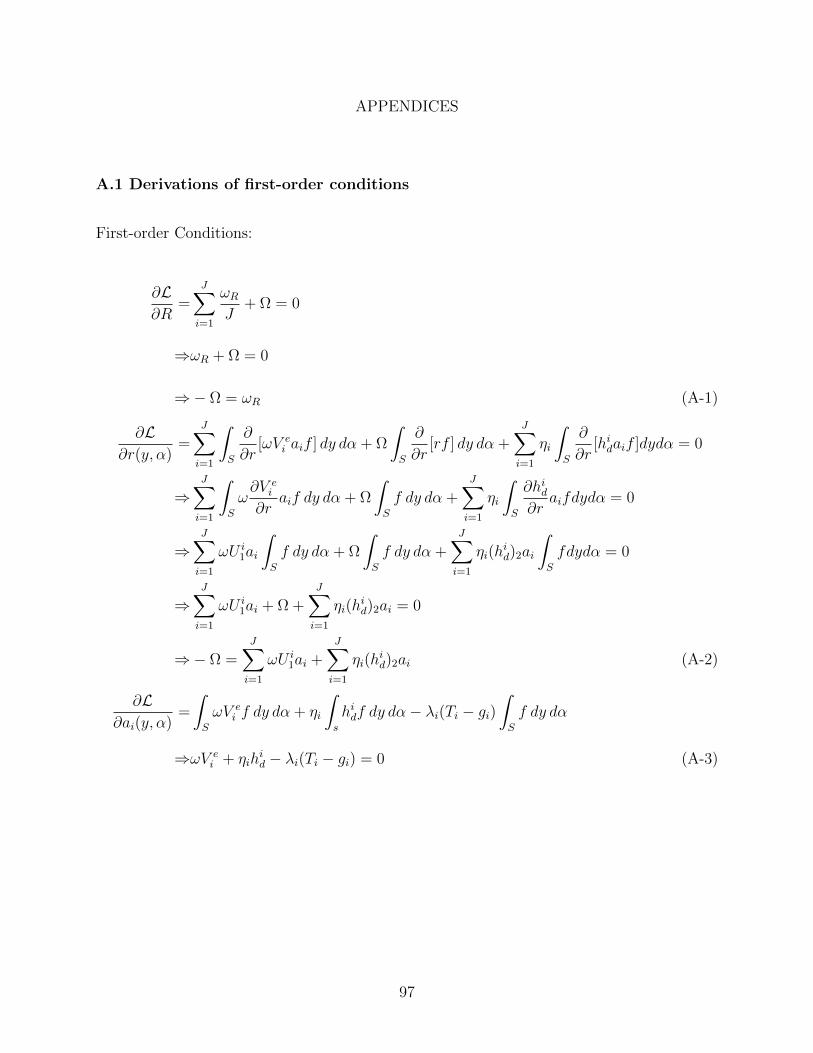
APPENDICES

A.1 Derivations of first-order conditions

First-order Conditions:

∂L∂R

=J∑i=1

ωRJ

+ Ω = 0

⇒ωR + Ω = 0

⇒− Ω = ωR (A-1)

∂L∂r(y, α)

=J∑i=1

∫S

∂

∂r[ωV e

i aif ] dy dα + Ω

∫S

∂

∂r[rf ] dy dα +

J∑i=1

ηi

∫S

∂

∂r[hidaif ]dydα = 0

⇒J∑i=1

∫S

ω∂V e

i

∂raif dy dα + Ω

∫S

f dy dα +J∑i=1

ηi

∫S

∂hid∂r

aifdydα = 0

⇒J∑i=1

ωU i1ai

∫S

f dy dα + Ω

∫S

f dy dα +J∑i=1

ηi(hid)2ai

∫S

fdydα = 0

⇒J∑i=1

ωU i1ai + Ω +

J∑i=1

ηi(hid)2ai = 0

⇒− Ω =J∑i=1

ωU i1ai +

J∑i=1

ηi(hid)2ai (A-2)

∂L∂ai(y, α)

=

∫S

ωV ei f dy dα + ηi

∫s

hidf dy dα− λi(Ti − gi)∫S

f dy dα

⇒ωV ei + ηih

id − λi(Ti − gi) = 0 (A-3)

97

∂L∂Ti

=− ωU i1

∫S

aif dy dα− ηi(hid)2

∫S

aif dy dα + λi

∫S

aif dy dα = 0

⇒− ωU i1 − ηi(hid)2 + λi = 0

⇒λi = ωU i1 + ηi(h

id)2 (A-4)

∂L∂ti

=ωR

(− piH

is

(1 + ti)2

)+

[−λi

H ispiti

(1 + t)2+ λi

H ispi

1 + ti− λi

p2i tiH

i′s

(1 + ti)3

]+ ηi

piHi′s

(1 + ti)2= 0

⇒− ωRpi

1 + ti+

[−λi

piti1 + t

+ λipi − λip2i ti

(1 + ti)2

H i′s

H is

]+ ηi

pi(1 + ti)

H i′s

H is

= 0

⇒− ωR +

[−λiti + λi(1 + ti)− λi

piti1 + ti

H i′s

H is

]+ ηi

(1 + ti)

pi

pi1 + ti

H i′s

H is

= 0

⇒− ωR +[λi − λitiεis

]+ ηi

(1 + ti)

piεis = 0

⇒− ωR + λi(1− tiεis) + ηi(H i

s)′

H is

= 0 (A-5)

∂L∂gi

=

∫S

ωU i3aif dy dα + ηi

∫S

(hid)3aif dy dα− λi∫S

aif dy dα = 0

⇒ωU i3Ni + ηi(h

id)3Ni − λiNi = 0 (A-6)

∂L∂g−i

=

∫S

ωU i4κaif dy dα + ηi

∫S

(hid)4δaif dy dα = 0

⇒ωU i4κNi + ηi(h

id)4δNi = 0

⇒ωU i4κ+ ηi(h

id)4δ = 0 (A-7)

98

∂L∂pi

=

∫S

−ωU i1h

idaif dy dα + ωR

H is

1 + ti

+ λi

[ti

1 + tiH is +

tipi1 + ti

H i′s

1 + ti

]+ ηi

∫S

(hid)1aif dy dα− ηiH i′s

1 + ti= 0

⇒−∫S

ωU i1h

idaif dy dα

1 + tiH is

+ ωR + λi

[ti +

tipi1 + ti

H i′s

H is

]+ ηi

∫S

(hid)1aif dy dα1 + tiH is

− ηiH i′s

1 + ti

1 + tiH is

= 0

⇒−∫S

ωU i1h

idaif dy dα

1 + tiH is


+ ηi

∫S

(hid)1aif dy dα1 + tiH is

− ηiH i′s

H is

= 0

⇒[ηi

∫S

(hid)1aif dy dα−∫S

ωU i1h

idaif dy dα

]1 + tiH is


− ηiH i′s

H is

= 0 (A-8)

99

A.2 Deriving equations for MATLAB functions1

The mean of income and the mean of preferences toward public goods are assumed having

lognormal distribution. Following (Heien, 1968), the mean, µ, of a variable X (in this case

X is income or preference) whereas X has a lognormal distribution (µx, σx) is:

µ = exp(µx +σ2x

2) (A-9)

Efficient Allocation

Assuming a CES utility function:

Ui = [βxxρ + βhh

ρ + βgi(α)gρi + βgj(α)κgρj ]1/ρ, (A-10)

where ρ < 0 and β′gi , βgj > 0. Let βg(α) ≡ α and βgj ≡ αj. Note that we suppress subscript

i on x and h for simplicity. Assuming the household preferences on public goods are the

same for i and j then we have:

Ui = [βxxρ + βhh

ρ + αgρi + ακgρj ]1/ρ (A-11)

Deriving indirect utility function

maxh

[βxxρ + βhh


1The equations are derived based on Epple and Sieg (1999) and a numerical simulation technique usedby Calabrese et al. (2012).

100

As an exponentiation is a monotone transformation, then we can change the problem into:

maxh

βxxρ + βhh

ρ + αgρi + ακgρj . (A-13)

First-order conditions:

−pβxρ(y − r − ph)ρ−1 + ρβhhρ−1 = 0

−pβx(y − r − ph)ρ−1 + βhhρ−1 = 0 (A-14)

Solving for hd (i.e. Marshallian demand for housing)— from A-14:

βhhρ−1 = pβx(y − r − ph)ρ−1

β1ρ−1

h h = p1ρ−1β

1ρ−1x (y − r − ph)

β1ρ−1

h h+ php1ρ−1β

1ρ−1x = (pβx)

1ρ−1 (y − r)

h(β1ρ−1

h + pρρ−1β

1ρ−1x ) = (pβx)

1ρ−1 (y − r)

hd =(pβx)

1ρ−1 (y − r)

β1ρ−1

h + pρρ−1β

1ρ−1x

×

[(1/βh)

1ρ−1

(1/βh)1ρ−1

]

hd =(pβx

βh)

1ρ−1 (y − r)

1 + (pρ βxβh

)1ρ−1

Dividing the numerator and the denominator with (pβxβh

)1ρ−1 , we obtain:

hd =y − r

(pβxβh

)1

1−ρ + p(A-15)

101

Substituting hd into the utility function to obtain the indirect utility function, Vi(pi, gi, gj):

Vi(.) = [βx(y − r − hd)ρ + βhhρd + αgρi + ακgρj ]

1/ρ

=

[βx(y − r −

(pβx

βh)

1ρ−1 (y − r)

1 + (pρ βxβh

)1ρ−1

)ρ + βh

(pβx

βh)

1ρ−1 (y − r)

1 + (pρ βxβh

)1ρ−1

ρ

+ αgρi + ακgρj

]1/ρ

=

[βx(y − r −

(pβx

βh)

1ρ−1 (y − r)

1 + (pρ βxβh

)1ρ−1

)ρ + βh

(pβxβh

)ρρ−1

[1 + (pρ βxβh

)1ρ−1 ]ρ

(y − r)ρ + αgρi + ακgρj

]1/ρ

=

[βx((y − r)(1−

(pβxβh

)1ρ−1

1 + (pρ βxβh

)1ρ−1

))ρ + βh(pβx

βh)

ρρ−1

[1 + (pρ βxβh

)1ρ−1 ]ρ


]1/ρ

=

[βx(y − r)ρ(1−

(pβxβh

)1ρ−1

1 + (pρ βxβh

)1ρ−1

)ρ + βh(pβx

βh)

ρρ−1

[1 + (pρ βxβh

)1ρ−1 ]ρ


]1/ρ

=

[βx(y − r)ρ(

1

1 + (pβxβh

)1ρ−1

)ρ + βh(pβx

βh)

ρρ−1

[1 + (pρ βxβh

)1ρ−1 ]ρ


]1/ρ

(A-16)

We can then rewrite A-16 as:

V (.) = [(y − r)ρΦ(p) + αgρi + ακgρj ]1/ρ (A-17)

where Φ(p) = βx

1+(p βxβh

)1ρ−1

+βh(p βx

βh)ρρ−1

[1+(pρ βxβh

)1ρ−1 ]ρ

.

102

The boundary locus between jurisdiction i and j satisfies:

Vi(pi, gi, κgj) = Vj(pj, gj, κgi)

⇒ [(y − ri)ρΦ(pi) + αgρi + ακgρj ]1/ρ = [(y − rj)ρΦ(pj) + αgρj + ακgρi ]

1/ρ

⇒ α =(y − rj)ρΦ(pj)− (y − ri)ρΦ(pi)

gρi − gρj + κ(gρj − g

ρi )

(A-18)

⇒ ln αij(y) = ln[(y − rj)ρΦ(pj)− (y − ri)ρΦ(pi)


ρi )

](A-19)

To calculate community populations and incomes, we use the result from Epple and Sieg

(1999) to get the standardized value of the joint distribution (ln y, lnα), Z, by utilizing A-19:

Zij(y) =ln[

(y−rj)ρΦ(pj)−(y−ri)ρΦ(pi)

gρi−gρj+κ(gρj−g

ρi )

]− µlnα − λσlnα

ln y−µln y

σlny

σlnα

√1− λ2

(A-20)

Following Epple and Sieg (1999) for Matlab function zproca:

µln(α)| ln(y) = µln(α) + λσln(α)

lny − µln(y)

σln(y)

(A-21)

σln(α)| ln(y) = σln(α)

√1− λ2 (A-22)

Zi =lnα− µlnα| ln y − σ2

lnα| ln y

σlnα| ln y(A-23)

Deriving the pivotal voter locus

In this model, we assume that households maximize their utility by consuming housing with

respect to public good provision in their own jurisdiction since they vote only for taxation

in the jurisdiction where they live.

Denoting hd as the pivotal voters housing demand in equilibrium, then the utility

103

function in equilibrium is:

Ui = [βx(y − ri − pihid)ρ + βhhidρ

+ αgρi + ακgρj ]1/ρ (A-24)

FOC(gi) :dUidgi

=1

ρ[βx(y − ri − pihid)

ρ + βhhidρ

+ αgρi + ακgρj ]1ρ−1

× [ρβx(y − ri − pihid)ρ−1(−dri

dgi− dpidgi

) + ραgρ−1i ] = 0

104

Assuming dridgi

= 0 and dpidgi

= 1, then:

− ρβx(y − ri − phid)ρ−1 + ραgρ−1

i = 0

⇒ αi(y) =βx(y − ri − pihid)ρ−1

gρ−1i

substituting A-15 for hid :

αi(y) =

βx

(y − ri − pi

(pi

βxβh

)1ρ−1 (y−r)

1+(pρiβxβh

)1ρ−1

)ρ−1

gρ−1i

=

βx

(y − ri − pi(pi βxβh )

1ρ−1

(y−r)

1+(pρiβxβh

)1ρ−1

)ρ−1

gρ−1i

=

βx

(y − ri − (pρi

βxβh

)1ρ−1

(y−r)

1+(pρiβxβh

)1ρ−1

)ρ−1

gρ−1i

=

βx

(y[1+

(pρi

βxβh

)1ρ−1 ]

[1+(pρiβxβh

)1ρ−1 ]−

r[1+

(pρiβxβh

)1ρ−1 ]

[1+(pρiβxβh

)1ρ−1 ]−

(pρiβxβh

)1ρ−1 (y−ri)

[1+(pρiβxβh

)1ρ−1 ]

)ρ−1

gρ−1i

αi(y) =

βx

(y−r

1+(pρiβxβh

)1ρ−1

)ρ−1

gρ−1i

(A-25)

and consequently:

lnα(y) = ln

[βx( y−r

1+(pρiβxβh

)1ρ−1

)ρ−1

gρ−1i

]

= ln βx − (ρ− 1)[ln(1 + (pρβxβh

)1ρ−1 )) + ln g + (ρ− 1) ln(y − r)]

105

or we can relate to the procedure used in Calabrese et al. (2012):

lnα = Ki + (ρ− 1) ln(y − r)

where

Ki = ln(βx)− (ρ− 1)

ln(

1 + (pρβxβh

)1ρ−1

)+ ln gi

(A-26)

Standardized values for pivotal voter based on Epple and Sieg (1999) then:

Zi(y) =lnα− µlnα − λσlnα

ln y−µln y

σlny

σln y

√1− λ2

=Ki + (ρ− 1) ln(y − r)− µlnα − λσlnα

ln y−µln y

σlny

σln y

√1− λ2

(A-27)

106

Tiebout allocation

Assuming a CES utility function:

Ui = [βxxρ + βhh

ρ + βgi(α)gρi + βgj(α)κgρj ]1/ρ, (A-28)

where ρ < 0 and β′gi , βgj > 0. Let βg(α) ≡ α and βgj ≡ αj. Note that we suppress subscript

i on x and h for simplicity. Assuming the household preferences on public goods are the

same for i and j then we have:

Ui = [βxxρ + βhh


Deriving indirect utility function

maxh

[βxxρ + βhh


As an exponentiation is a monotone transformation, then we can change the problem into:

maxh

βxxρ + βhh

ρ + αgρi + ακgρj . (A-31)


−pβxρ(y − ph)ρ−1 + ρβhhρ−1 = 0

−pβx(y − ph)ρ−1 + βhhρ−1 = 0 (A-32)

107

Solving for hd (i.e. Marshallian demand for housing)— from A-32:

βhhρ−1 = pβx(y − ph)ρ−1

β1ρ−1

h h = p1ρ−1β

1ρ−1x (y − ph)

β1ρ−1

h h+ php1ρ−1β

1ρ−1x = (pβx)

1ρ−1y

h(β1ρ−1

h + pρρ−1β

1ρ−1x ) = (pβx)

1ρ−1y

hd =(pβx)

1ρ−1y

β1ρ−1

h + pρρ−1β

1ρ−1x

×

[(1/βh)

1ρ−1

(1/βh)1ρ−1

]

hd =(pβx

βh)

1ρ−1y

1 + (pρ βxβh

)1ρ−1

Dividing the numerator and the denominator with (pβxβh

)1ρ−1 , we obtain:

hd =y

(pβxβh

)1

1−ρ + p(A-33)

108

Substituting hd into the utility function to obtain the indirect utility function, Vi(pi, gi, gj):

Vi(.) = [βx(y − hd)ρ + βhhρd + αgρi + ακgρj ]

1/ρ

=

[βx(y −

(pβx

βh)

1ρ−1y

1 + (pρ βxβh

)1ρ−1

)ρ + βh

(pβx

βh)

1ρ−1y

1 + (pρ βxβh

)1ρ−1

ρ

+ αgρi + ακgρj

]1/ρ

=

[βx(y −

(pβx

βh)

1ρ−1 (y − r)

1 + (pρ βxβh

)1ρ−1

)ρ + βh

(pβxβh

)ρρ−1

[1 + (pρ βxβh

)1ρ−1 ]ρ

yρ + αgρi + ακgρj

]1/ρ

=

[βx(y(1−

(pβxβh

)1ρ−1

1 + (pρ βxβh

)1ρ−1

))ρ + βh(pβx

βh)

ρρ−1

[1 + (pρ βxβh

)1ρ−1 ]ρ


]1/ρ

=

[βxy

ρ(1−(pβx

βh)

1ρ−1

1 + (pρ βxβh

)1ρ−1

)ρ + βh(pβx

βh)

ρρ−1

[1 + (pρ βxβh

)1ρ−1 ]ρ


]1/ρ

=

[βxy

ρ(1

1 + (pβxβh

)1ρ−1

)ρ + βh(pβx

βh)

ρρ−1

[1 + (pρ βxβh

)1ρ−1 ]ρ


]1/ρ

=

[yρ

βx

[1 + (pβxβh

)1ρ−1 ]ρ

+ yρβh(p

βxβh

)ρρ−1

[1 + (pρ βxβh

)1ρ−1 ]ρ

+ αgρi + ακgρj

]1/ρ

(A-34)

We can then rewrite A-34 as:

V (.) = [yρΦ(p) + αgρi + ακgρj ]1/ρ (A-35)

where Φ(p) = βx

1+(p βxβh

)1ρ−1

+βh(p βx

βh)ρρ−1

[1+(pρ βxβh

)1ρ−1 ]ρ

.

109

The boundary locus between jurisdiction i and j satisfies:

Vi(pi, gi, κgj) = Vj(pj, gj, κgi)

⇒ [yρΦ(pi) + αgρi + ακgρj ]1/ρ = [yρΦ(pj) + αgρj + ακgρi ]

1/ρ

⇒ αij =yρΦ(pj)− yρΦ(pi)


ρi )

=yρ(Φ(pj)− Φ(pi))


ρi )

(A-36)

⇒ lnαij(y) = ln[ yρ(Φ(pj)− Φ(pi))


ρi )

](A-37)

We can rewrite as:

lnαij(y) = ρ ln y +Kij (A-38)

where Kij = ln[ (Φ(pj)− Φ(pi))


ρi )

](A-39)

Kij is the community intercept or variable kint in the matlab program.

Following Epple and Sieg (1999) to get the standardized value of the joint distribution

(ln y, lnα), Z(y):

Zij(y) = Ωj + ω ln(y) (A-40)

where ωj = ω1 + ω2

ω1 =ρ

σα√

1− λ2

ω2 =−λ

σln y

√1− λ2

Ω =Kj − µlnα + λσlnα

µln y

σln y

σln y

√(1− λ2)

110

Deriving the pivotal voter locus

The next step is deriving the pivotal voter locus. In this model, we assume that households

maximize their utility by consuming houses with respect to public good provision in their

own jurisdiction since they vote only for taxation in the jurisdiction where they live.

Denoting hd as the pivotal voters housing demand in equilibrium, then the utility

function in equilibrium is:

Ui = [βx(y − pihid)ρ + βhhidρ

+ αgρi + ακgρj ]1/ρ (A-41)

FOC(gi) :dUidgi

=1

ρ[βx(y − pihid)

ρ + βhhidρ

+ αgρi + ακgρj ]1ρ−1

× [−ρβx(y − pihid)ρ−1dpi

dgihid + ραgρ−1

i ] = 0

⇒ [−ρβx(y − pihid)ρ−1dpi

dgihd + ραgρ−1

i ] = 0

⇒ dp

dg=

αgρ−1

βx(y − phid)ρ−1hid(A-42)

111

Substituting A-33 to A-42:

dp

dg=

αgρ−1

βx(y − p[

(p βxβh

)1ρ−1 y

1+(pρ βxβh

)1ρ−1

])ρ−1

[(p βxβh

)1ρ−1 y

1+(pρ βxβh

)1ρ−1

]=

αgρ−1

βx(y −[

(pρ βxβh

)1ρ−1 y

1+(pρ βxβh

)1ρ−1

])ρ−1

[(p βxβh

)1ρ−1 y

1+(pρ βxβh

)1ρ−1

]=

αgρ−1

βx(y[1−[

(pρ βxβh

)1ρ−1

1+(pρ βxβh

)1ρ−1

]])ρ−1

[(p βxβh

)1ρ−1 y

1+(pρ βxβh

)1ρ−1

]=

αgρ−1

βx(y[

1

1+(pρ βxβh

)1ρ−1

])ρ−1

[(p βxβh

)1ρ−1 y

1+(pρ βxβh

)1ρ−1

]=

αgρ−1

βxyρ−1 1

[1+(pρ βxβh

)1ρ−1 ]ρ−1

[(p βxβh

)1ρ−1

1+(pρ βxβh

)1ρ−1

]y

=αgρ−1

βxyρ[

(p βxβh

)1ρ−1

1+(pρ βxβh

)1ρ−1

] =αgρ−1

βxyρ

1+(pρ βxβh

)1ρ−1

(pβxβh

)1ρ−1

=αgρ−1[

y

1+(pρ βxβh

)1ρ−1

]ρβ

ρρ−1x

(βhp

) 11−ρ

=αgρ−1[

y

1+(pρ βxβh

)1ρ−1

]ρβ

ρρ−1x

(βhp

) ρ1−ρ βh

p

=αgρ−1[

y

1+(pρ βxβh

)1ρ−1

(βhp

) 11−ρβ

1ρ−1x

]ρβhp

=αgρ−1[

y

1+(pρ βxβh

)1ρ−1

(βhpβx

) 11−ρ]ρ

βhp

(A-43)

112

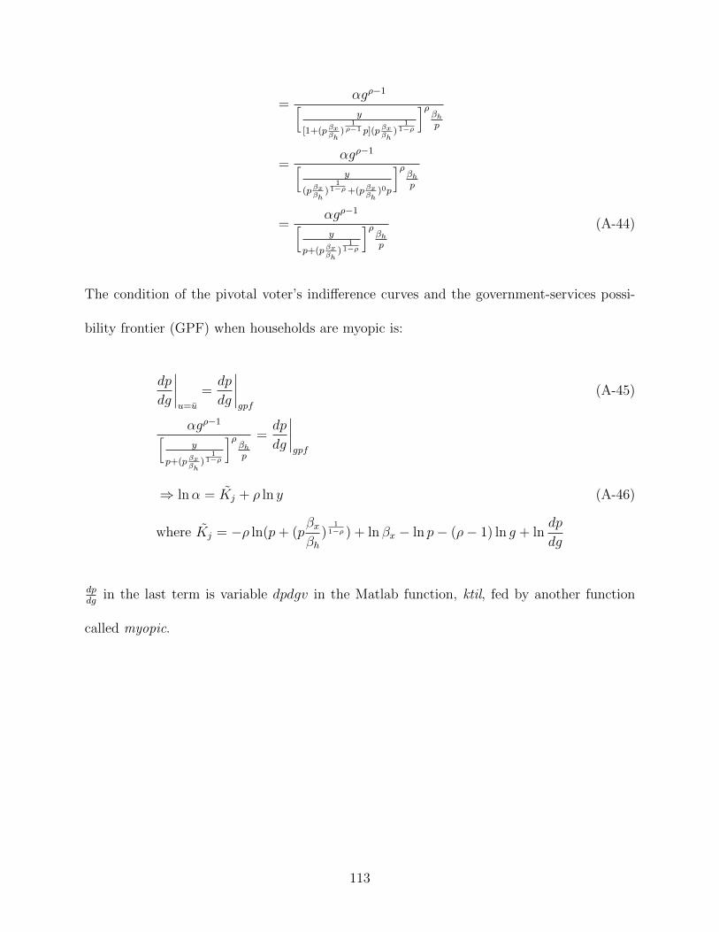
=αgρ−1[y

[1+(p βxβh

)1ρ−1 p](p βx

βh)

11−ρ

]ρβhp

=αgρ−1[y

(p βxβh

)1

1−ρ+(p βxβh

)0p

]ρβhp

=αgρ−1[y

p+(p βxβh

)1

1−ρ

]ρβhp

(A-44)

The condition of the pivotal voter’s indifference curves and the government-services possi-

bility frontier (GPF) when households are myopic is:

dp

dg

∣∣∣∣u=u

=dp

dg

∣∣∣∣gpf

(A-45)

αgρ−1[y

p+(p βxβh

)1

1−ρ

]ρβhp

=dp

dg

∣∣∣∣gpf

⇒ lnα = Kj + ρ ln y (A-46)

where Kj = −ρ ln(p+ (pβxβh

)1

1−ρ ) + ln βx − ln p− (ρ− 1) ln g + lndp

dg

dpdg

in the last term is variable dpdgv in the Matlab function, ktil, fed by another function

called myopic.

113

A.3 Matlab codes

HEAD TAX

This Matlab program is written based on GAUSS program used by Calabrese et al.

(2012). There are 5 communities in the metropolitan area that impose an efficient tax (head-

tax). Although we assume absentee landlords, we take into account their welfare in the CV

calculation.

The main script below will call ten functions (procedures): func.m, kcalc.m, zproc.m,

zproca.m, summrs.m,poproc.m, inproc.m, cvcalc.m, montc.m, and nlsrch.m.

%% Main script

clear all;

clc;

%% set sample size for Monte Carlo simulation

smpl=1000000;

%% generate repeatable random number with the Mersenne twister generator

s = RandStream(’mt19937ar’,’Seed’,1); % MATLAB’s start-up settings

RandStream.setDefaultStream(s);

%% FOR MATLAB2013 users:

% rng(1,’twister’);

% s=rng;

eps1=randn(smpl,1);

eps2=randn(smpl,1);

kappa_vec=0:0.1:1; %kappa is a parameter of public good spillovers

pot_gain=zeros(1,length(kappa_vec));

for iii=1:length(kappa_vec)

kappa=kappa_vec(iii);

%for ii=1:length(pot_gain)

114

warning off; % turning off Warnings on GLOBAL VARIABLE

ncom=5; % Number of communities

Montind=1; %Montind=1 to do Monte Carlo comparison

%% Parameters

muy= 10.51710439;

sigy= 0.88623;

mual= -2.36406786786;

sigal= 0.00990949382558 ;

lam = 0;

gm=.25;

ALx= 1;

wq =1;

Theta = (1-gm)/gm;

ALh =0.355945238972 ;

rho = -.01;

%% I use "for loop" to create a plot of kappa vs. potential welfare gain

land=[.4 .15 .15 .15 .15]’;

zmin =ones(1,48)*(-1000);

lnalphamax = ones(1,48)*10;

hsuply=ones(ncom,1);

iter=0;

bigind=0;

iwrite=0;

nlfac=1;

big=100;

global ncom kappa muy sigy mual sigal lam gm ALx wq Theta ALh rho yvec...

lyvec lnalphamax diff wvec iwrite tol bignum maxits nlfac big ibig bigind...

land mual zmin wvec smpl eps1 eps2 gc;

incnu=ones(ncom,1);

popn=ones(ncom,1);

hd=ones(ncom,1);

%dpdgv=ones(ncom,1);

meanincandalpha=[exp(muy+sigy^2/2) exp(mual+sigal^2/2)];

display(’mean income and alpha’); disp(num2str(meanincandalpha))

115

%% From Calabrese et.al. (2012):

%% evec is a vector of ordinates for numerical integration where the values

%% are normalized to the interval (-1,+1). If a function of a variable x

%% is to be integrated over an interval [xl,xh], the ordinates

%% normalized to that interval are obtained by

%% x=(0.5*((xl+xh)+(diff.*evec’))) where diff=xh-xl.

evec=[...

-0.9987710 -0.9935302 -0.9841246 -0.9705916 -0.9529877,-0.9313867,...

-0.9058791 -0.8765720 -0.8435883 -0.8070662 -0.7671590,-0.7240341,...

-0.6778724 -0.6288674 -0.5772247 -0.5231610 -0.4669029 -0.4086865,...

-0.3487559 -0.2873625 -0.2247638 -0.1612224 -0.0970047 -0.03238017,...

0.03238017 0.09700470 0.1612224 0.2247638 0.2873625 0.3487559,...

0.40868650 0.46690290 0.5231610 0.5772247 0.6288674 0.6778724,...

0.72403410 0.76715900 0.8070662 0.8435883 0.8765720 0.9058791,...

0.93138670 0.95298770 0.9705916 0.9841246 0.9935302 0.9987710]’ ;

%% Wvec is a vector of interval widths normalized to conform to the

%% normalization of evec. To renormalize to an interval [xl,xh],

%% multiply by diff/2 where diff=xh-xl.

wvec=[...

0.00315335 0.00732755 0.01147723 0.01557932 0.01961616 0.02357076,...

0.02742651 0.03116723 0.03477722 0.03824135 0.04154508 0.04467456,...

0.04761666 0.05035904 0.05289019 0.05519950 0.05727729 0.05911484,...

0.06070444 0.06203942 0.06311419 0.06392424 0.06446616 0.06473770,...

0.06473770 0.06446616 0.06392424 0.06311419 0.06203942 0.06070444,...

0.05911484 0.05727729 0.05519950 0.05289019 0.05035904 0.04761666,...

0.04467456 0.04154508 0.03824135 0.03477722 0.03116723 0.02742651,...

0.02357076 0.01961616 0.01557932 0.01147723 0.00732755 0.00315335]’ ;

xl=-5;

xh=3;

diff=xh-xl;

lyvec=muy +sigy*(0.5*((xl+xh)+(diff.* evec’)));

yvec=exp(lyvec);

kmin=xl;

yvec=repmat(yvec,ncom,1); %% transform yvec from 1x48 into 5x48

116

%% initial guess

x0=[10 10 10 10 10 1832 4623 6544 9626 17371 1832 4623 6544 9626 17371]’;

%% Centralized property-tax equilibrium values

pc = [17.1321740284 17.1321740284 17.1321740284 17.1321740284...

17.1321740284]’;

capqc = (((1+((pc.^rho)*ALx/ALh).^(1/(rho-1))).^rho).^(-1))*ALx +...

ALh*(pc*ALx/ALh).^(rho/(rho-1)))./(1+((pc.^rho)*ALx/ALh).^(1/...

(rho-1))).^rho;

tc =[.35 .35 .35 .35 .35]’;

gc =[3829.71688669 3829.71688669 3829.71688669 3829.71688669...

3829.71688669]’;

iwrite=0;

tol=.000001;

maxits=1000;

nlfac=1;

dh=1e-4;

iter=1000;

big=1000;

ibig=0;

bignum=.125;

bigind=0;

nladj=1.05;

%%======================Loop========================%%

xsave = x0;

x=xsave;

count=ones(size(x,1),1);

icnt=0;

while icnt<size(count,1);

icnt=icnt+1;

count(icnt,1)=icnt;

end;

allfun=abs(func(x));

maxfun=max(allfun);% create a row vector with max values for each column

nladj=1.05;

if maxfun<20;

117

nladj=1.5;

end

dh=.0001;

nlfac=.05;

x = nlsrch(x,tol,bignum,maxits,nlfac);

xsave=x;

funcout=func(x);

pr=[ncom muy sigy mual sigal lam ALh ALx rho gm Theta];

disp(’parameters:’);

disp(’ncom’ ’muy’ ’sigy’ ’mual’ ’sigal’ ’lam’ ’ALh’ ’ALx’ ’rho’...

’gm’ ’Theta’

’kappa’; ncom muy sigy mual sigal lam ALh ALx rho gm Theta kappa);

disp(’result p, g t are’); %% t is a headtax or r in in this program

p=x(1:ncom,1);

g=x(ncom+1:2*ncom,1);

r=x(2*ncom+1:3*ncom,1);

disp(num2str([p g r]))

kv=kcalc(p,g,r,yvec,lyvec);

zmat=zproc(kv,lyvec);

inc=inproc(zmat);

popn=poproc(zmat);

display(’Incomes, Populations, Mean Incomes’)

disp(num2str([inc popn inc./popn]))

display(’Sum of Community Incomes Compared to Total Metropolitan Income’)

disp(num2str([sum(inc) exp(muy+sigy^2/2)]))

hd = (p+(ALx*p./ALh).^(1/(1-rho))).^(-1).*(inc-r.*popn);

hsuply=land.*p.^Theta*((1-gm)/wq).^Theta;

display(’Housing Demands and Supplies, housing share of income,...

Land Areas’)

disp(num2str([hd,hsuply,p.*hd./inc,land]))

118

if Montind==1;

[kvrnd,yave,houave]=montc([p;g;r],capqc);

monres=[kvrnd yave houave];

display(’Compare Monte Carlo and quadrature’)

display(’Community Sizes’)

disp(num2str([monres(:,1) popn]))

display(’community mean incomes’)

disp(num2str([monres(:,2) (inc./popn)]))

display(’mean housing demand’)

disp(num2str([monres(:,3),hd./popn]))

[avgcvad,distbetad] = cvcalc([p;g;r],capqc);

cvdist=[avgcvad,distbetad];

disp(’avgcv and %better off’);

disp(num2str([avgcvad; distbetad]))

rentsa =gm*((1-gm)/wq).^((1-gm)/gm)*sum(land.*(pc./(1+tc)).^(1/gm))’;

rentsb = gm*((1-gm)/wq).^((1-gm)/gm)*sum(land.*p.^(1/gm))’;

display(’ Rents a, b ’)

disp(num2str( [rentsa,rentsb]))

Rentsch= rentsb - rentsa;

display(’ Change in Rents=’)

disp(num2str(Rentsch))

display(’aggregate cv + change in rents’);

disp(num2str(cvdist(1,1)-Rentsch))

pot_gain(iii)=-((cvdist(1,1)-Rentsch));

end

h=plot(kappa_vec,pot_gain)

set(h,’linewidth’,2);

title(’Spillover vs. Potential Gain, A Head-Tax Case (US)’)

xlabel(’\kappa’)

119

ylabel(’Potential gain (US$)’)

%% this is the end of the main script

120

%% func.m

function[fun]=func(x)

global ncom gm ALx wq Theta ALh rho yvec lyvec iwrite nlfac big bigind land;

xs=x;

fun=zeros(3*ncom,1);

p=x(1:ncom,1);



kv=kcalc(p,g,r,yvec,lyvec);


zmata = zproca(kv,lyvec);

popn=poproc(zmat);

incnu=inproc(zmat);

hd = (p+(ALx*p./ALh).^(1/(1-rho))).^(-1).*(incnu-r.*popn);

if iwrite <100;

iwrite=iwrite+1;

elseif iwrite>09;

iwrite=0;

nlfac=min([1; 1.05*nlfac],[],1); % it will return a min value

% between 1 and 1.05*nlfac

display(’nlfac big ibig’ nlfac big bigind);

end

hsuply=land.*p.^Theta.*((1-gm)/wq).^Theta;

summrsxg = summrs(p,g,r,yvec,lyvec,zmata);

fun(1:ncom,1)=hd-hsuply;

fun(ncom+1:2*ncom,1)=r-g;

fun(2*ncom+1:3*ncom,1)=summrsxg-popn;

x=xs;

fun;

end

%% this is the end of func.m

121

%% kcalc.m

function[lnalpha]=kcalc(pvect,gvec,rvec,yvec,lyvec)

global ALx ALh rho yvec lyvec lnalphamax ncom kappa;

rvec=repmat(rvec,1,48);

pvect=repmat(pvect,1,48);

aty = (yvec-rvec);

%%capq is ncomx48

capq=(aty.^rho).*(ALx./(1+(pvect.^rho*ALx/ALh).^(1/(rho-1))).^rho +...

(ALh*(pvect*ALx/ALh).^(rho/(rho-1)))./(1+(pvect.^rho*ALx/ALh).^(1/...

(rho-1))).^rho);

%% alpha is 4x48

alpha=(capq(2:ncom,:)-capq(1:(ncom-1),:))./repmat((gvec(1:...

(ncom-1),1).^rho-gvec(2:ncom,1).^rho)+kappa*((gvec(2:ncom,1).^rho-gvec...

(1:(ncom-1),1).^rho)),1,48);

% Repmat replicate the denominator from 4x1 into 4x48;

% divide numerator with the denominator element by element.

lnalpha = log(alpha);

lnalpha(imag(lnalpha)~=0)= 10;

lnalpha = [lnalpha; lnalphamax];

end

%% this is the end of kcalc.m

122

%% zproc.m

function[zv]= zproc(kv,lyv)

global ncom muy sigy mual sigal lam;

%% I use repmat to generate a (ncomx48) matrix with uniform values.

omgv = (kv./(sigal*(1-lam^2).^(.5)))-repmat((mual/(sigal*(1-lam^2).^(.5...

))),ncom,48)-lam*((repmat(lyv,ncom,1)-repmat(muy,ncom,48...

))./sigy)./(1-lam^2).^(.5);

zv=omgv;

end

%% this the end of zproc.m

%% zproca.m

function[zv]= zproca(kv,lyv)

global ncom muy sigy mual sigal lam ;

mualy = repmat(mual,1,48)+lam*sigal.*(lyv-repmat(muy,1,48)./sigy); %% 1x48

sigaly = sqrt(1-lam.^2)*sigal; %% scalar

zv= (kv-repmat(mualy,ncom,1)-repmat(sigaly.^2,ncom,48))./sigaly;

zv;

end

%% this is the end of zproca.m

123

%% summrs.m

function[summrsxg]=summrs(p,g,r,yv,lyv,zmata)

global mual ncom lam sigal muy sigy rho ALx ALh zmin diff wvec;

mualy = mual+lam*sigal.*((lyv-muy)./sigy);

sigaly = sqrt(1-lam^2)*sigal;

r=repmat(r,1,48);

p=repmat(p,1,48);

g=repmat(g,1,48);

capq = g.^(rho-1)./((ALx.*((yv-r)-(p.*(yv-r))./(p+(p.*ALx/ALh).^(1/...

(1-rho)))).^(rho-1)));

capq(isnan(capq))= 0;

capq(imag(capq)~=0)=0;

zmatb = [zmin;zmata(1:(ncom-1),:)];

summrsxg= (diff/2)*((repmat(exp(mualy+sigaly^2/2),ncom,1).*...

(normcdf(zmata)-normcdf(zmatb)).*capq).*repmat(normpdf((lyv-muy)/...

sigy),ncom,1)*wvec);

end

%% this is the end of summrs.m

%%poproc.m

function[popn]=poproc(zmat)

global ncom muy sigy lyvec diff wvec;

%% zmat is 5x48, where 5=ncom

cumpop=(diff/2).*(repmat(normpdf((lyvec-repmat(muy,1,48))/sigy),ncom,1)...

).*normcdf(zmat)*wvec;

cumpop=[0;cumpop];

popn=(cumpop(2:(ncom+1),1)-cumpop(1:ncom,1));

end

%% this is the end of poproc.m

124

%%inproc.m

function[incnu]=inproc(zmat)


cincnu=((diff/2).*repmat(exp(lyvec).*normpdf((lyvec-...

repmat(muy,1,48))/sigy),ncom,1).*normcdf(zmat)*wvec);

cincnu=[0;cincnu];

incnu=(cincnu(2:(ncom+1),1)-cincnu(1:ncom,1));

end

%% this is the end of inproc.m

125

%% cvcalc.m

function[avgcvad,distbetad]=cvcalc(x,capqc)

global smpl ncom ALx ALh rho muy sigy lam eps1 eps2 mual sigal gc kappa;

cv=zeros(smpl,1);

p=x(1:ncom,1);



capq=ALx./(1+((p.^rho)*ALx/ALh).^(1./(rho-1))).^rho +...

ALh*(p*ALx/ALh).^(rho/(rho-1)))./(1+((p.^rho)*ALx/ALh).^(1/(rho-1))).^rho;

yrnd=exp(muy+sigy*((1-lam^2).^(.5))*eps1+lam*sigy*eps2);

alprnd=exp(mual+sigal*eps2);

utlc = (repmat(alprnd’,5,1).*repmat(gc,1,1000000).^rho+kappa*repmat...

(alprnd’,5,1).*repmat(gc,1,1000000).^rho+repmat(capqc,1,1000000).*repmat...

(yrnd’,5,1).^rho).^(1/rho);

utl=(repmat(alprnd’,5,1).*repmat(g,1,1000000).^rho+kappa*repmat...

(alprnd’,5,1).*repmat(g,1,1000000).^rho+repmat(capq,1,1000000).*(repmat...

(yrnd,1,5)-repmat(r’,1000000,1))’.^rho).^(1/rho);

cvall = ((utlc.^rho - repmat(alprnd’,5,1).*repmat(g,1,1000000).^rho-...

kappa*repmat(alprnd’,5,1).*repmat(g,1,1000000).^rho)./repmat...

(capq,1,1000000)).^(1/rho)-(repmat(yrnd,1,5)-repmat(r’,1000000,1))’;

ordstat2=min(cvall,[],1)’;

%% Return the minimum of matrix cvall from each column,

%% and put them as a COLUMN vector

avgcvad= sum(ordstat2)’/smpl;

distadad = logical(ordstat2<=0);

distbetad = sum(distadad)’/smpl;

end

%% this is the end of cvcalc.m

126

%% montc.m

function[kvrnd,yave,houave]=montc(x,capqc)

global smpl ncom ALx ALh rho muy sigy lam eps1 eps2 mual sigal gc kappa;

cv=zeros(smpl,1);

p=x(1:ncom,1);



capq=ALx./(1+((p.^rho)*ALx/ALh).^(1/(rho-1))).^rho +...

(ALh*(p*ALx/ALh).^(rho/(rho-1)))./(1+((p.^rho)*ALx/ALh).^(1/(rho-1))).^rho;

yrnd=exp(muy+sigy*((1-lam^2).^.5)*eps1+lam*sigy*eps2);


utl=-(repmat(alprnd’,5,1).*repmat(g,1,1000000).^rho+kappa*repmat...

(alprnd’,5,1).*repmat(g,1,1000000).^rho+repmat...

(capq,1,1000000).*(repmat(yrnd,1,5)-repmat(r’,1000000,1))’.^rho);

utlc = (repmat(alprnd’,5,1).*repmat(gc,1,1000000).^rho+kappa*repmat...

(alprnd’,5,1).*repmat(gc,1,1000000).^rho+...

repmat(capqc,1,1000000).*repmat(yrnd’,5,1).^rho).^(1/rho);

cv = ((utlc.^rho - repmat(alprnd’,5,1).*repmat(g,1,1000000).^rho-...

kappa*repmat(alprnd’,5,1).*repmat(g,1,1000000).^rho)./repmat...

(capq,1,1000000)).^(1/rho)-(repmat(yrnd,1,5)-repmat(r’,1000000,1))’;

ordstat1=min(cv,[],1)’;

%% Return the minimum of a matrix cv from each column

avgcv = sum(ordstat1)’/smpl;

e1=logical(repmat(ordstat1,1,5)==cv’);

kvrnd=sum(e1)’/smpl;

yave=(sum(e1.*repmat(yrnd,1,5))’/smpl)./kvrnd;

houave=(p+(ALx*p./ALh).^(1/(1-rho))).^(-1).*(sum(e1.*(repmat(yrnd,1,5)-...

repmat(r’,1000000,1)))’/smpl)./kvrnd;

end

%% this is the end of montc.m

127

%% nlsrch.m

% Note that I have 2 local functions in this particular script:grad1 and bv

function[x1]=nlsrch(x0,tol,bignum,maxits,nlfac)

global big bigind ibig

k=size(x0,1);

fv0=func(x0);

dx=1; iter=1; big=1000; ibig=0;

option1=0; option2=1; option3=1; option4=1;

if option4 == 0;

disp(’******** Solution of Non-Linear Equation System *********** ’);

end;

tic;

while (abs(dx)>=tol & iter <= maxits & big >= tol)

jc=grad1(fv0,x0,k);

x1=x0 - nlfac*inv(jc)*fv0;

% evaluate the vector function with the new estimates

fv1=func(x1);

% Compute the largest function value in the vector of functions

big=max(abs(fv1));

% Define the index of the largest function value in the vector of functions.

[saka,Indices]=max(abs(fv1)); ibig=Indices’ ;

%%Define index for which function is largest.

[arana,index]=max(abs(fv1)); bigind=index’;

if big<bignum;

nlfac=max([((bignum-.95*big)/bignum);nlfac])’;

end;

128

if option1 == 1;

disp([’Iteration = ’ num2str(iter)])

disp([’f(x0) = ’]); disp([ num2str(fv0)]);

disp([’New estimates = ’]); disp([num2str(x1)]);

end;

if option2 == 1;

if abs(fv1) > abs(fv0);

disp(’The procedure is diverging. The current values are: ’)

disp([’Iteration = ’ num2str(iter)])

disp([’f(x0) = ’]); disp([ num2str(fv0)])



disp([’x1 = ’]); disp([ num2str(x1)])

disp(’ Try new starting values. ’);

end;

end;

dx=x1-x0; x0=x1;

fv0=func(x0);

iter=iter + 1;

end;

big=max(abs(fv1))’;

if option4 == 0; %

disp([’Largest element of Abs(f(x)) is: ’ num2str(big)])

end;

if iter > maxits;

129

disp(’Iteration limit exceeded:’);

disp([’Largest element of Abs(f(x)) is: ’ num2str(big)])

disp([’Final estimates for x are: ’]); disp([num2str(x1)])

end;

if option3 == 1;

tme=toc

if option4==0;

disp([’Total time required: ’ num2str(tme) ’seconds’])

disp([’Total number of iterations:’ num2str(iter-1)])

end;

end;

end

%%Jacobian matrix

function[g]=grad1(gf0,gx0,k);

dh=1e-4;

g=zeros(k,k);

i=1;

while i<=k;

g(:,i)=(func(bv(gx0,1,i,k))-gf0)/dh;

i=i+1;

end;

end

function[bv_output]=bv(b,a,i,k)

gee=eye(k); %%% k=15 , gee is an identity matrix 15x15

dh=1e-4;

bv_output=b+(a*dh)*gee(:,i);

end

%% this is the end of nlsrch.m

130

PROPERTY TAX

This Matlab program is written based on GAUSS program used by Calabrese et al.

(2012). There are 5 communities in the metropolitan area with property tax. Although we

assume absentee landlords, we take into account their welfare in the CV calculation. We

assume lognormal distributions for both income and preference parameter for public good.

As in Calabrese et al. (2012) we also assume that voters are myopic.

The main script below will call ten functions (procedures): myopic.m, trans.m, un-

trans.m, func.m, kcalc.m, ktil.m, zproc.m, voproc.m, poproc.m, inproc.m, cvcalc.m, montc.m,

and nlsrch.m. Note that nlsrch.m used in this program is the same as nlsrch.m used in the

head tax case.

clear all;

clc;

warning off; %%% turning off Warnings on GLOBAL VARIABLE

ncom=5; % Number of communities

%% creating repeatable random number with the mersenne twister generator



%% Set following to 1 to do Monte Carlo comparison%%

kappa_vec=0:0.1:0.9;

pot_gain=zeros(1,length(kappa_vec));

tax_vec=zeros(ncom, length(kappa_vec));

perc_better=zeros(1,length(kappa_vec));

popn_vec=zeros(ncom, length(kappa_vec));

meaninc_vec=zeros(ncom, length(kappa_vec));

for iii=1:length(kappa_vec)

kappa=kappa_vec(iii);

131

Montind=1;

%%Initial Parameters%%

muy=10.51710439;

sigy=0.88623;

mual = -2.36406786786;

sigal= 0.00990949382558 ;

lam = 0;

gm=.25;

ALx= 1;

wq =1;

Theta = (1-gm)/gm;

ALh =0.355945238972 ;

rho = -.01;

land=[.4 .15 .15 .15 .15]’;

omg1=0;

omg2=0;

gex=0;

kmax=10;

hsuply=ones(ncom,1);

iter=0;

iloop=0;

mxt=100*ones(ncom,1);

bigind=0;

parad=0;

iwrite=0;

nlfac=1;

bigpct=100;

big=100;

taxbal=.2*ones(ncom,1);

global kappa ncom muy sigy mual sigal lam gm ALx wq Theta ALh rho yvec...

lyvec diff wvec iwrite nlfac tol bignum maxits big ibig bigind land mual...

wvec smpl eps1 eps2 gc mxt kmax;

incnu=ones(ncom,1);

popn=ones(ncom,1);

hd=ones(ncom,1);

132

dpdgv=ones(ncom,1);

meanincandalpha=[exp(muy+sigy^2/2) exp(mual+sigal^2/2)];

display(’mean income and alpha’); disp(num2str(meanincandalpha))

%% From Calabrese et.al. (2012):

% evec is a vector of ordinates for numerical integration. These

% ordinates are normalized to the inteval (-1,+1).

% if a function of a variable x is to be integrated over an interval

% [xl,xh], the ordinates normalized to that interval are obtained by

% x=(0.5*((xl+xh)+(diff.*evec’))) where diff=xh-xl.

evec=[...

-0.9987710 -0.9935302 -0.9841246 -0.9705916 -0.9529877,-0.9313867,...

-0.9058791 -0.8765720 -0.8435883 -0.8070662 -0.7671590,-0.7240341,...

-0.6778724 -0.6288674 -0.5772247 -0.5231610 -0.4669029 -0.4086865,...

-0.3487559 -0.2873625 -0.2247638 -0.1612224 -0.0970047 -0.03238017,...

0.03238017 0.09700470 0.1612224 0.2247638 0.2873625 0.3487559,...

0.40868650 0.46690290 0.5231610 0.5772247 0.6288674 0.6778724,...

0.72403410 0.76715900 0.8070662 0.8435883 0.8765720 0.9058791,...

0.93138670 0.95298770 0.9705916 0.9841246 0.9935302 0.9987710]’ ;

%% Wvec is a vector of interval widths normalized to conform to the

% normalization of evec above. To renormalize to an interval [xl,xh],

% 5 multiply by diff/2 where diff=xh-xl.

wvec=[...

0.00315335 0.00732755 0.01147723 0.01557932 0.01961616 0.02357076,...

0.02742651 0.03116723 0.03477722 0.03824135 0.04154508 0.04467456,...

0.04761666 0.05035904 0.05289019 0.05519950 0.05727729 0.05911484,...

0.06070444 0.06203942 0.06311419 0.06392424 0.06446616 0.06473770,...

0.06473770 0.06446616 0.06392424 0.06311419 0.06203942 0.06070444,...

0.05911484 0.05727729 0.05519950 0.05289019 0.05035904 0.04761666,...

0.04467456 0.04154508 0.03824135 0.03477722 0.03116723 0.02742651,...

0.02357076 0.01961616 0.01557932 0.01147723 0.00732755 0.00315335]’ ;

xl=-5;

xh=3;

diff=xh-xl;

lyvec=muy +sigy*(0.5*((xl+xh)+(diff.* evec’)));

yvec=exp(lyvec);

133

kmin=xl;

%% Initial guess

x0=[ 14.258...

16.185...

17.175...

18.391...

20.797...

1880.980...

3063.992...

3849.785...

5006.582...

8016.818...

0.3488...

0.3507...

0.3518...

0.3529...

0.3545]’;

%% Centralized property-tax equilibrium values

pc = [17.1321740284 17.1321740284 17.1321740284 17.1321740284...

17.1321740284]’;

capqc = (((1+((pc.^rho)*ALx/ALh).^(1/(rho-1))).^rho).^(-1))*ALx +...

(ALh*(pc*ALx/ALh).^(rho/(rho-1)))./...

(1+((pc.^rho)*ALx/ALh).^(1/(rho-1))).^rho;

tc =[.35 .35 .35 .35 .35]’;

gc =[3829.71688669 3829.71688669 3829.71688669 3829.71688669...

3829.71688669]’;

% Set sample size for Monte Carlo simulation

% generate repeatable random number with the Mersenne twister generator



%% FOR MATLAB2013 users:

% rng(1,’twister’);

% s=rng;

smpl=1000000;

134

eps1=randn(smpl,1);

eps2=randn(smpl,1);

iwrite=0;

tol=1e-8;

maxits=100;

nlfac=1;

dh=1e-4;

iter=1000;

big=1000;

ibig=0;

bignum=.125;

bigind=0;

nladj=1.05;

%% ============Loop==============

xsave=trans(x0);

x=xsave;

count=ones(size(x,1),1);

icnt=0;

while icnt<size(count,1);

icnt=icnt+1;

count(icnt,1)=icnt;

end;

allfun=abs(func(x));

maxfun=max(allfun);

nladj=1.05;

if maxfun<20;

nladj=1.5;

end

dh=.001;

nlfac=.05;

x = nlsrch(x,tol,bignum,maxits,nlfac);

xsave=x;

funcout=func(x);

135

x=untrans(x);

pr=[ncom muy sigy mual sigal lam ALh ALx rho gm Theta];

disp(’parameters:’);

disp(’ncom’ ’muy’ ’sigy’ ’mual’ ’sigal’ ’lam’ ’ALh’ ’ALx’ ’rho’...

’gm’ ’Theta’ ’kappa’;

ncom muy sigy mual sigal lam ALh ALx rho gm Theta kappa);

disp(’result p, g, t are’);

p=x(1:ncom,1);


tax=x(2*ncom+1:3*ncom,1);

disp(num2str([p g tax]))

kv=kcalc(p,g);


inc=inproc(zmat);

popn=poproc(zmat);

display(’Incomes, Populations, Mean Incomes’)

disp(num2str([inc popn inc./popn]))

%% ?;

display(’Sum of Community Incomes Compared to Total Metropolitan Income’)

disp(num2str([sum(inc) exp(muy+sigy^2/2)]))

hd = (p+(ALx*p./ALh).^(1/(1-rho))).^(-1).*inc;

hsuply=land.*(p./(1+tax)).^Theta*((1-gm)/wq).^Theta;

%%?;

display(’Housing Demands and Supplies, housing share of income,...

Land Areas’)

disp(num2str([hd,hsuply,p.*hd./inc, land]))

if Montind==1;

[kvrnd,yave,houave]=montc([p;g]);

monres=[kvrnd yave houave];

display(’Compare Monte Carlo and quadrature’)

136

display(’Community Sizes’)

disp(num2str([monres(:,1) popn]))

display(’community mean incomes’)

disp(num2str([monres(:,2) (inc./popn)]))

display(’mean housing demand’)

disp(num2str([monres(:,3),hd./popn]))

[avgcvad,distbetad] = cvcalc([p;g],capqc);

cvdist=[avgcvad,distbetad];

disp(’aggregate cv and %better off’);

disp(num2str([avgcvad; distbetad]))

rentsa =gm*((1-gm)/wq).^((1-gm)/gm)*sum(land.*(pc./(1+tc)).^(1/gm))’;

rentsb = gm*((1-gm)/wq).^((1-gm)/gm)*sum(land.*(p./(1+tax)).^(1/gm))’;

display(’ Rents a, b ’)

disp(num2str( [rentsa,rentsb]))

Rentsch= rentsb - rentsa;

display(’ Change in Rents=’)

disp(num2str(Rentsch))

display(’aggregate cv + change in rents’);

disp(num2str(cvdist(1,1)-Rentsch))

pot_gain(iii)=-((cvdist(1,1)-Rentsch));

tax_vec(:,iii)=tax;

perc_better(iii)=distbetad;

popn_vec(:,iii)=popn;

meaninc_vec(:,iii)=inc./popn;

end

%% Plot kappa vs.potential gain

figure;

h0=plot(kappa_vec,pot_gain);

set(h0,’linewidth’,2);

ylim([-600 0]);

xlim([0 0.9]);

title(’Spillover vs. Potential Gain, A Property Tax Case (US)’);

xlabel(’\kappa’);

137

ylabel(’Potential gain (US$)’);

%% Plot kappa vs. property tax

figure;

tax_vec_conv=0.07*tax_vec;

h=plot(kappa_vec,tax_vec_conv);

set(h,’linewidth’,2);

title(’Spillover vs. Property tax rate (US)’);


ylabel(’Property tax’);

legend(’Central City’,’Suburban1’,’Suburban2’,’Suburban3’,’Suburban4’,

’Location’, ’SouthWest’);

%% Plot kappa vs. distbetad

better=100*perc_better;

figure;

h2=plot(kappa_vec,better);


ylim([-100 100]);

xlim([0 0.9]);

title(’Spillover vs. Better-off, a property tax case (US)’);


ylabel(’Better-off population (%)’);

%% Plot kappa vs. Population

figure;

h3=plot(kappa_vec,popn_vec);


title(’Spillover vs. Population, a property tax case (US)’);


ylabel(’Population (normalized to 1)’)


’Location’,’Northeast’);

%% Plot kappa vs. Mean Incomes

figure;

h4=plot(kappa_vec,meaninc_vec);


title(’Spillover vs. Mean incomes, a property tax case (US)’);

138


ylabel(’Mean Incomes’);


’Location’,’SouthWest’);

%% this is the end of the main script for property tax

139

%% kcalc.m

function [kint] = kcalc(pvect,gvec)

global kappa ALx ALh rho kmax;

capq=ALx./(1+(pvect.^rho*ALx/ALh).^(1/(rho-1))).^rho+...

(ALh*(pvect*ALx/ALh).^(rho/(rho-1)))./(1+(pvect.^rho*ALx/ALh).^(1/...

(rho-1))).^rho;

kint=log((capq(2:5,1)-capq(1:4,1))./(gvec(1:4,1).^rho-gvec(2:5,1).^rho+...

kappa*(gvec(2:5,1).^rho-gvec(1:4,1).^rho)));

kint=[kint;kmax];

kint(imag(kint)~=0)= 10;

kint(isnan(kint)) = 10;

kint(isinf(kint)) = 10;

end

%% this is the end of kcalc.m

%% ktil.m

function [ktilde] = ktil(p,g,dpdgv)

global rho ALx ALh

ktilde=-rho*log(p+(p*(ALx/ALh)).^(1/(1-rho)))+log(ALh)-log(p)-...

(rho-1)*log(g)+log(dpdgv);

ktilde(imag(ktilde)~=0)= 10;

ktilde(isnan(ktilde)) = 10;

ktilde(isinf(ktilde)) = 10;

end

%% this is the end of ktil.m

140

%% zproc.m

function [zv] = zproc(kv,lyv)

global muy sigy mual sigal lam rho ;

omg1=rho./(sigal*(1-lam^2)^.5);

omg2=-lam./(sigy*(1-lam^2)^.5);

omgv=(kv-mual+lam*sigal*muy/sigy)./(sigal*(1-lam^2)^.5);

zv=repmat(omgv,1,48)+(omg1+omg2)*repmat(lyv,5,1);

%% zv is 5x48. it’s zmat in the main script

end

%% this is the end of zproc.m

%% voproc.m

function [ vlow ] = voproc(zmat,ztmat)

global ncom diff lyvec muy sigy wvec;

zlolim=-5*ones(1,size(zmat,2));

zlobnd=[zlolim;zmat(1:(ncom-1),:)];

vlow=((diff/2).*(repmat((normpdf(((lyvec-muy)/sigy))),5,1).*...

(normcdf(ztmat)-normcdf(zlobnd))*wvec));

end

%% this is the end of voproc.m

141

%% poproc.m

function [popn] = poproc(zmat)


% zmat is 5x48, where 5=ncom

cumpop=(diff/2).*(repmat(normpdf((lyvec-repmat(muy,1,48))/...

sigy),ncom,1)).*normcdf(zmat)*wvec;

cumpop=[0;cumpop];

popn=(cumpop(2:6,1)-cumpop(1:5,1));

end

%% this is the end of poproc.m

%% inproc.m

function[incnu]=inproc(zmat)


cincnu=((diff/2).*repmat(exp(lyvec).*normpdf((lyvec-repmat(muy,1,48))/...

sigy),ncom,1).*normcdf(zmat)*wvec);

cincnu=[0;cincnu];

incnu=(cincnu(2:6,1)-cincnu(1:5,1));

end

%% this is the end of inproc.m

%% myopic.m

function [myop] = myopic(hd,popn)

% This proc calculates the slope of the GPF when voters are myopic

myop=popn./hd;

end

%% this is the end of myopic.m

142

%% cvcalc.m

function [avgcv,distbet,avgcvad,distbetad] = cvcalc(x,capqc)

global kappa smpl ncom ALx ALh rho muy sigy lam eps1 eps2 mual sigal gc;

p=x(1:ncom,1);


capq=ALx./(1+((p.^rho)*ALx/ALh).^(1./(rho-1))).^rho +...


yrnd=exp(muy+sigy*((1-lam^2).^(.5))*eps1+lam*sigy*eps2);


utlc = (repmat(alprnd’,5,1).*repmat(gc,1,1000000).^rho-kappa*...

repmat(alprnd’,5,1).*repmat(gc,1,1000000).^rho+repmat(capqc,1,1000000).*...

repmat(yrnd’,5,1).^rho).^(1/rho);

utl=(repmat(alprnd’,5,1).*repmat(g,1,1000000).^rho-kappa*...

repmat(alprnd’,5,1).*repmat(g,1,1000000).^rho+repmat(capq,1,1000000).*...

(repmat(yrnd,1,5))’.^rho).^(1/rho);

cvall = ((utlc.^rho - repmat(alprnd’,5,1).*repmat(g,1,1000000).^rho...

-kappa*repmat(alprnd’,5,1).*repmat(g,1,1000000).^rho)./...

repmat(capq,1,1000000)).^(1/rho)-(repmat(yrnd,1,5))’;

ordstat1=max(utl)’;

cv=zeros(smpl,1);

icmax =smpl;

icnt = 0;

while icnt < icmax;

icnt = icnt + 1;

jvar=0;

while jvar<5;

jvar=jvar+1;

if utl(jvar,icnt) == ordstat1(icnt,1);

cv(icnt,1) = ((utlc(jvar,icnt).^rho -...

alprnd(icnt,1)*g(jvar,1).^rho)/capq(jvar,1)).^(1/rho)-yrnd(icnt,1);

end

143

end;

end;

avgcv= sum(cv)’./smpl;

dist=logical(cv<0);

distbet = sum(dist)’/smpl;

ordstat2=min(cvall,[],1)’;

%% Return the minimum of matrix cvall from each column

avgcvad= sum(ordstat2)’/smpl;

distadad = logical(ordstat2<=0);

distbetad = sum(distadad)’/smpl;

end

%% this is the end of cvcalc.m

144

%% montc.m

function [kvrnd,yave,houave] = montc(x,capqc)

global kappa smpl ncom ALx ALh rho muy sigy lam eps1 eps2 mual sigal gc;

p=x(1:ncom,1);


capq=ALx./(1+((p.^rho)*ALx/ALh).^(1/(rho-1))).^rho +...


yrnd=exp(muy+sigy*((1-lam^2).^.5)*eps1+lam*sigy*eps2);


utl=-(repmat(alprnd’,5,1).*repmat(g,1,1000000).^rho-kappa*...

repmat(alprnd’,5,1).*repmat(g,1,1000000).^rho+repmat(capq,1,1000000).*...

(repmat(yrnd,1,5))’.^rho);

ordstat1=max(utl)’;

e1=logical(repmat(ordstat1,1,5)==utl’);

kvrnd=sum(e1)’/smpl;

yave=(sum(e1.*repmat(yrnd,1,5))’/smpl)./kvrnd;

%% this is the end of montc.m

We use the same program and procedures for Indonesian case with different param-

eters and initial guess for head-tax case. To calibrate the Indonesian property tax case we

use the results from the head tax case and calibrate the housing prices to get a condition

where the housing market is in an equilibrium.

%PARAMETER FOR INDONESIAN CASE

muy= 9.861407405811761; %Statistic Indonesia, Jakarta 2011

sigy= 0.8310;

145

%% Initial guess:

x0=[10 10 10 10 10 952 2403 3402 5005 9032 952 2403 3402 5005 9032]’;

%%Centralized property-tax equilibrium values%%

pc = [13.1321740284 13.1321740284 13.1321740284 13.1321740284...

13.1321740284]’;

tc=[0.1 0.1 0.1 0.1 0.1]’;

gc =[2129.71688669 2129.71688669 2129.71688669 2129.71688669...

2129.71688669]’;

146

A.4 Comparison between Monte Carlo and Quadrature Results

A.4.1 Efficient Tax

Table A.1: Comparison: Community size

Jurisdiction Monte Carlo Quadrature

1 0.54 0.532 0.12 0.163 0.16 0.134 0.13 0.115 0.06 0.07

Table A.2: Comparison: Mean incomes


1 21836.59 21514.202 46122.16 47369.653 65445.85 69464.264 107345.43 103512.535 232143.27 203572.87

Table A.3: Comparison: Mean housing demand


1 482.07934 474.468962 875.58096 900.977893 1190.347 1268.90824 1879.7208 1808.06075 3791.4179 3296.2473

147

A.4.2 Property Tax

Table A.4: Comparison: Community size


1 0.42 0.392 0.15 0.153 0.15 0.154 0.14 0.155 0.14 0.16

Table A.5: Comparison: Mean incomes


1 27873.14 26954.372 45695.17 43692.873 57352.55 54753.884 74584.73 71008.765 122386.04 113309.55

Table A.6: Comparison: Housing demand


1 524.60 507.302 759.64 726.353 899.58 858.824 1093.76 1041.325 1589.32 1471.45

148

A.5 The household’s maximization problem

maxxia,x

ib,liπiu[U

iu(x

ia, x

ib, li)] + πid[U

id(x

ia, x

ib, li)]

subject to

qaxia + qbx

ib = wili(1− ti)σi + wili(1− σi)− Ti

Where qa = pa(1 + τa) then we can rewrite the constraint as:

pa(1 + τa) + qbxib = wili(1− σiti)− Ti

Assuming:

U iu > U i

d

U iu − U i

d = G(1− σi)wili(1− σi)

τb = 0

⇒ πiu[Uiu(xa, xb, li)] + πid[U

id(xa, xb, li)] = (1− πid)[U i

u(xa, xb, li)] + πid[Uid(xa, xb, li)]

= U iu(.)− πid[U i

u(.)− U id(.)]

= U iu(.)− πidG(1− σi)wili[1− σi]

149

Define g(1− σi) ≡ G(1− σi)(1− σi) as cost of being detected per unit income, we have:

πiu[Uiu(.)] + πid[U

id(.)] = U i

u(.)− πidg(1− σi)wili

The maximization problem:

maxxia,x

ib,liU iu(.)− πidg(1− σi)wili s.t. pa(1 + τa)x

ia + qbx

ib = wili(1− tiσi)− Ti

It gives us the Lagrangian function as follows:

L = U iu(xa, xb, li)− πidg(1− σi)wili + α[wili(1− tiσi)− Ti − (1 + τa)x

ia − qbxib]

By Roy’s identity we obtain:

V iτa =

dU

dτa=∂L∂τa

∣∣∣∣∗

= −αixia

V iti

=dU

dti=∂L∂ti

∣∣∣∣∗

= −αiwiliσi

V iTi

=dU

dTi=∂L∂Ti

∣∣∣∣∗

= −αi

V iσi

=dU

dσi=∂L∂σi

∣∣∣∣∗

= −wili(πidg′(1− σi) + αiti)

where αi is the marginal utility of income, both pa and pb(= qb) are numeraire.

150

A.6 The mimicker’s maximization problem

Defining:

l2 ≡w1l1w2

σ2 ≡σiwiliw2l2

x2a(τa, t1, T1; l2, σ2)

x2b(τa, t1, T1; l2, σ2)

V 2(τa, t1, T1) ≡ U2(x2a(.), x

2b(.),

w1l1(.)

w2

; σ2)

The maximization problem for a mimicker:

maxx2a,x

2b ,l2U(x2

a, x2b , l2)− π2

dg(1− σ2)w2l2 s.t. w2l2(1− t1σ2)− T1 − x2a(1 + τa)− x2

b

which gives a Lagrangian function:

L = U(x2a, x

2b ,w1l1w2

)− π2dg(1− σ2)w2l2 + α2[w2l2(1− t1σ2)− T1 − x2

a(1 + τa)− x2b ]

L = U(.)− π2dg(1− σ2)w2

w1l1(.)

w2

+ α2[w2w1l1(.)

w2

(1− t1σ2)− T1 − x2a(1 + τa)− x2

b ]

L = U(.)− π2dg(1− σ2)w1l1(.) + α2[w1l1(.)(1− t1σ2)− T1 − x2

a(1 + τa)− x2b ]

151

By the envelope theorem:

V 2τa =

∂L∂τa

∣∣∣∣∗

=Ul2w2

∂w1l1∂τa

− π2dg(1− σ2)

∂w1l1∂τa

+ α2

[(1− t1σ2)

∂w1l1∂τa

− x2a

]V 2t1

=∂L∂t1

∣∣∣∣∗

=Ul2w2

∂w1l1∂t1

− π2dg(1− σ2)

∂w1l1∂t1

+ α2

[− w1l1σ2 + (1− t1σ2)

∂w1l1∂t1

]V 2T1

=∂L∂T1

∣∣∣∣∗

=Ul2w2

∂w1l1∂T1

− π2dg(1− σ2)

∂w1l1∂T1

+ α2

[(1− t1σ2)

∂w1l1∂T1

− 1

]V 2σ2

=∂L∂σ2

∣∣∣∣∗

= −(π2dg′(1− σ2)w1l1 + α2w1l1t1)

Please note that we also assume g(0) = g′(0) = 0.

We can then rewrite the equations into:

V 2τa = −α2x

2a + α2∂w1l1

∂τaξ

V 2t1

= −α2w1l1σ2 + α2∂w1l1∂t1

ξ

V 2T1

= −α2 + α2∂w1l1∂T1

ξ

V 2τ2

= −w1l1(α2t1 + π2dg′(1− τ2))

where

ξ ≡Ul2w2α2

+ (1− t1σ2)− π2dg(1− σ2)

α2

152

A.7 The planner’s problem

Before working on the planner’s problem we will derive equations of compensated labor

supply and demand for good a (denoted by a tilde). Defining household i tax payment:

Ri = τaxia + t1σiwili + Ti

⇒ wili = (Ri − τaxia − Ti)1

tiσi

⇒ ∂wili∂Ri

= −∂wili∂Ti

=1

tiσi

Defining duality and adopting Cook (1972):

wili(ti, Ui) ≡ wili(ti, Ri, (ti, U

i))

∂wili∂ti

=∂wili∂ti

+∂wili∂Ri

.∂Ri

∂ti

∂wili∂ti

=∂wili∂ti− ∂wili

∂Ti.σiwili

Analogously, utilizing the same process for compensated demand for good a, where the

duality is xia(ti, Ui) ≡ xia(ti, Ri(ti, U

i)), we can obtain:

∂xia∂ti

=∂xia∂ti− wiliσi

∂wili∂Ti

153

Now we turn to the maximization problem.

The planner faces a maximization problem as follows:

maxτa,ti,Ti

V 2(τa, t2, T2)

subject to:

MUC : V 1(τa, t1, T1) ≥ U1s

ICH : V 2(τa, t2, T2) ≥ V 2(τa, t1, T1;w1l1(.)

w2

)

GBC : n1[τax1a(.) + σ1t1w1l1(.) + T1] + n2[τax

2a(.) + τ2t2w2l2(.) + T2] ≥ R0

where x1a(τa, t1, T1), x2

a(τa, t2, T2), l1(τa, t1, T1), and l2(τa, t2, T2).

µ, λ > 0 since we have monotonic preferences, and γ > 0 if U1s is sufficiently high. It is also

assumed that we have a normal case (see Stiglitz, 1982), i.e. the low type will never mimic

high type.

The Lagrangian function:

L = V 2(τa, t2, T2) + µ

[U1s − V 1(τa, t1, T1)

]+ γ

[V 2(τa, t1, T1;

w1l1(.)

w2

)

−V 2(τa, t2, T2)

]+ λ

[R0 − n1[τax

1a(τa, t1, T1) + σ1t1w1l1(τa, t1, T1) + T1]− n2[τax

2a(τa, t2, T2)

+τ2t2w2l2(τa, t2, T2) + T2]

]

154


∂L∂τa

=V 2τa − µV

1τa + γV 2

τa − γV2τa + λ

[− n1

(τa∂x1

a

∂τa+ x1

a + t1σ1∂w1l1∂τa

)− n2

(τa∂x2

a

∂τa+ x2


)]= 0

∂L∂t1

=− µV 1t1

+ γV 2t1

+ λ

[− n1

(τa∂x1

a

∂t1+ t1σ1

∂w1l1∂t1

+ σ1w1l1

)]= 0

∂L∂t2

=V 2t2− γV 2

t2+ λ

[− n2

(τa∂x2

a

∂t2+ t2σ2

∂w2l2∂t2

+ σ2w2l2

)]= 0

∂L∂T1

=− µV 1T1

+ γV 2T1

+ λ

[− n1

(τa∂x1

a

∂T1

+ t1σ1∂w1l1∂T1

+ 1

)]= 0

∂L∂T2

=V 2T2− γV 2

T2+ λ

[− n2

(τa∂x2

a

∂T2

+ t2σ2∂w2l2∂T2

+ 1

)]= 0

155

Using some manipulations:

(i) foc(t1)− w1l1σ1foc(T1) = 0

− µV 1t1

+ γV 2t1− λn1

(τa∂x1

a

∂t1+ t1σ1

∂w1l1∂t1

+ σ1w1l1

)− w1l1σ1

[− µV 1

T1+ γV 2

T1− λn1

(τa∂x1

a

∂T1

+ t1σ1∂w1l1∂T1

+ 1

)]= 0

⇒− µV 1t1

+ γV 2t1− λn1τa

∂x1a

∂t1− λn1t1σ1

∂w1l1∂t1

−((((((λn1σ1w1l1

+ w1l1σ1µV1T1− w1l1σ1γV

2T1

+ w1l1σ1λn1τa∂x1

a

∂T1

+ w1l1σ1λn1t1σ1∂w1l1∂T1

+((((((w1l1σ1λn1 = 0

⇒t1(λn1σ1

[∂w1l1∂t1

− σ1w1l1∂w1l1∂T1

])= −µV 1

t1+ γV 2

t1− λn1τa

∂x1a

∂t1+ w1l1σ1µV

1T1

− w1l1σ1γV2T1


a

∂T1

⇒t1(λn1σ1

∂w1l1∂t1

)= −µ(V 1

t1− w1l1σ1V

1T1

) + γ

[(((

(((−α2w1l1σ1 + α2∂w1l1∂t1

ξ

]− λn1τa

∂x1a

∂t1− w1l1σ1γ

[−α2 + α2

∂w1l1∂T1

ξ

]+ w1l1σ1λn1τa

∂x1a

∂T1

Since the first term on the RHS equals to zero by the first-order condition of households’

maximization problem, then we obtain:

⇒ t1

(λn1σ1

∂w1l1∂t1

)= γξα2

(∂w1l1∂t1

− w1l1σ1∂w1l1∂T1

)− λn1τa

(∂x1

a

t1− w1l1σ1

∂w1l1∂T1

)= γξα2

∂w1l1∂t1

− λn1τa∂x1

a

t1

⇒ t1 =γα2

λn1σ1

ξ − τaσ1

∂x1a/∂t1

∂w1l1/∂t1

156

(ii) foc(t2)− w2l2σ2foc(T2) = 0

V 2t2− γV 2

t2− λn2τa

∂x2a

∂t2− λn2t2σ2

∂w2l2∂t2

− λn2σ2w2l2

− w2l2σ2

[V 2T2− γV 2

T2− λn2τa

∂x2a

∂T2

− λn2t2σ2∂w2l2∂T2

− λn2

]= 0

⇒V 2t2− γV 2

t2− λn2τa

∂x2a

∂t2− λn2t2σ2

∂w2l2∂t2

−((((((λn2σ2w2l2

− w2l2σ2V2T2

+ w2l2σ2γV2T2


a

∂T2

+ w2l2σ2λn2t2σ2∂w2l2∂T2

+((((((w2l2σ2λn2 = 0

⇒(1− γ)(V 2t2− w2l2σ2V

2T2

)− λn2τa

(∂x2

a

∂t2− w2l2σ2

∂w2l2∂T2

)= t2λn2σ2

(∂w2l2∂t2

− w2l2σ2∂w2l2∂T2

)

Again, the first term in the second parentheses equals to zero by the previous first-order

conditions of households’ maximization problem.

⇒t2λn2σ2∂w2l2∂t2

= −λn2τa∂x2

a

∂t2

⇒t2 =∂x2

a/∂t2


157

(iii) foc(τa)− x1afoc(T1)− x2

afoc(T2) = 0

V 2τa − µV

1τa + γV 2

τa − γV2τa − λn1

[τa∂x1

a

∂τa+ x1


]− λn2

[τa∂x2

a

∂τa+ x2

a

+ t2σ2∂w2l2∂τa

]+ x1

a

[µV 1

T1− γV 2

T1+ λn1τa

∂x1a

∂T1

+ λ1n1t1σ1∂w1l1∂T1

+ λn1

]− x2

a

[V 2T2− γV 2

T2− λn2τa

∂x2a

∂T2

− λn2t2σ2∂w2l2∂T2

+ λn2

]= 0

⇒−α2x2a +

µα1x1a + γ

[− α2x

2a + α2

∂w1l1∂τa

ξ

]+

γα2x2a − λn1τa

∂x1a

∂τa−

λn1x1a − λn1t1σ1

∂w1l1∂τa

− λn2τa∂x2

a

∂τa−

λn2x2a − λn2t2σ2

∂w2l2∂τa

−x1

aµα1 − x1aγ

[− α2 + α2

∂w1l1∂T1

ξ

]+ x1

aλn1τa∂x1

a

∂T1

+ x1aλn1t1σ1

∂w1l1∂T1

+x1

aλn1 +x2

aα2 + x2aγ[−α2] + x2

aλn2τa∂x2

a

∂T2

+ x2aλn2t2σ2

∂w2l2∂T2

+x2

aλn2 = 0

⇒− γα2x2a + γα2

∂w1l1∂τa

ξ − λn1τa∂x1

a

∂τa− λn1σ1

∂w1l1∂τa

[γα2

λn1σ1

ξ − τaσ1

∂x1a/∂t1

∂w1l1/∂t1

]− λn2τa

∂x2a

∂τa− λn2σ2

∂w2l2∂τa

[∂x2

a/∂t2


]+ x1

aγα2 − x1aα2

∂w1l1∂T1

ξ + x1aλn1τa

∂x1a

∂T1

+ x1aλn1σ1

∂w1l1∂T1

[γα2

λn1σ1

ξ − τaσ1

∂x1a/∂t1

∂w1l1/∂t1

]+ x2

aλn2τa∂x2

a

∂T2

+ x2aλn2σ2

∂w2l2∂T2

[∂x2

a/∂t2


]= 0

⇒− γα2x2a + γα2

∂w1l1∂τa

ξ − λn1τa∂x1

a

∂τa+ λn1σ1

∂w1l1∂τa

τa

σ1

∂x1a/∂t1

∂w1l1/∂t1−λn1σ1

∂w1l1∂τa

γα2

λn1σ1

ξ

− λn2τa∂x2

a

∂τa+ λn2σ2

∂w2l2∂τa

∂x2a/∂t2

∂w2l2/∂t2.τa

σ2

+ x1aγα2 − x1

aα2∂w1l1∂T1

ξ + x1aλn1τa

∂x1a

∂T1

− x1aλn1σ1

∂w1l1∂T1

τaσσ1

∂x1a/∂t1

∂w1l1/∂t1+ x1

aλn1σ1∂w1l1∂T1

γα2

λn1σ1

ξ

+ x2aλn2τa

∂x2a

∂T2

− x2aλn2σ2

∂w2l2∂T2

∂x2a/∂t2

∂w2l2/∂t2.τa

σ2

= 0

158

⇒− γα2xa2 +

γα2∂w1l1∂τa

ξ − λn1τa

[∂x1

a

∂τa− x1

a

∂x1a

T1

− ∂x1a/∂t1

∂w1l1/∂t1

(∂w1l1∂τa

− x1a

∂w1l1∂T1

)]−

∂w1l1

∂τaγα2ξ − λn2τa

[∂x2

a

∂τa− x2

a

∂x2a

T2

− ∂x2a/∂t2

∂w2l2/∂t2

(∂w2l2∂τa

− x2a

∂w2l2∂T2

)]+ x1

aγα2

−

x1aα2

∂w1l1∂T1

ξ +

x1aα2

∂w1l1∂T1

ξ = 0

Following Nava et.al (1996) that:

∂xia∂τa≡ ∂xia∂τa− xia

∂xiaTi

∂wili∂τa

≡ ∂wili∂τa

− xia∂wili∂Ti

∂xia∂τa

∣∣∣∣li

≡ ∂xia∂τa− ∂xia/∂ti

∂wili/∂ti

∂wili∂τa

,

then we can obtain:

⇒ −λτa[n1∂x1

a

∂τa

∣∣∣∣l1

+ n2∂x2

a

∂τa

∣∣∣∣l2

]= γα2(x2

a − x1a)

⇒ τa =γ

λα2(x1

a − x2a)

[n1∂x1

a

∂τa

∣∣∣∣l1

+ n2∂x2

a

∂τa

∣∣∣∣l2

]−1

159

DISSERTATION ESSAYS ON FISCAL DECENTRALIZATION AND …

Documents

Transcript of DISSERTATION ESSAYS ON FISCAL DECENTRALIZATION AND …