
Doctoral Dissertation Essays on Inflation Targeting THAN ...
143
Doctoral Dissertation Essays on Inflation Targeting THAN THAN SOE Graduate School for International Development and Cooperation Hiroshima University September 2018
Transcript of Doctoral Dissertation Essays on Inflation Targeting THAN ...
Doctoral Dissertation
Essays on Inflation Targeting
THAN THAN SOE
Graduate School for International Development and Cooperation
Hiroshima University
September 2018
Essays on Inflation Targeting
D165562
THAN THAN SOE
A Dissertation Submitted to
the Graduate School for International Development and Cooperation
of Hiroshima University in Partial Fulfillment
of the Requirement for the Degree of
Doctor of Philosophy
September 2018

i
Summary of dissertation
Inflation targeting (IT) regime has become a popular monetary policy framework across
countries. Since the early 1990’s, advanced countries have adopted an IT regime while
developing countries have adopted an IT regime since the late 1990’s. As of 2013, fourteen
advanced countries and fifteen developing countries have adopted an IT regime to achieve
better macroeconomic conditions. The main feature of an IT regime is an explicit inflation
target and strong central bank legal commitments to the transparency, accountability, and
credibility of price stability in conducting monetary policies (e.g., Mishkin, 2000; Mishkin
& Savastano, 2001). Policy makers expect that an IT regime may have favorable effects on
macroeconomic stability with low inflation and the stability of inflation and output. There
have existed many studies on the economic effects of this regime theoretically and
empirically. However, the adoption of IT may have several effects in various contexts. Thus,
this dissertation attempts to discuss how the IT adoption relates to three aspects: (i) income
velocity (domestic economy); (ii) exchange market pressure (external economy); (iii) central
bank credibility (institutional factor). This dissertation is composed of three studies: the first
study examines the impact of an IT regime on income velocity, the second study investigates
the impact of an IT regime on the exchange market pressure, and the third study analyses the
impact of an IT regime on credibility of the central bank.
The first study attempts to examine how inflation targeting relates to the variability
of income velocity and its components across 84 developing countries during the period
from 1990 to 2013. Developing economies tend to prefer or rely upon monetary policy rule
with monetary aggregates due to institutional constraints on monetary policy conduct.
Although inflation targeting has been adopted as an alternative monetary policy framework
in various developing countries, many developing countries are still adopting monetary
aggregates targeting due to unmatured money and financial markets. However, monetary

ii
aggregates targeting often fails to achieve the macroeconomic stability. One crucial
condition for monetary aggregates to be effective is the stability of income velocity. Income
velocity is more volatile in developing countries than in advanced countries so that stability
of income velocity is crucial to achieve macroeconomic stability under monetary aggregates
targeting. Taylor (2000) highlights that monetary targeting and inflation targeting can
coexist and monetary aggregates would be an appropriate instrument to achieve inflation
target in developing countries. If the adoption of IT stabilizes income velocity, monetary
authorities can justify monetary aggregates as an appropriate instrument under an IT regime.
Thus, the first study attempts to examine the relationship between an IT regime and income
velocity in developing countries. The results suggest that inflation targeting would help
stabilize income velocity in developing countries. In addition, a decomposition analysis of
income velocity generally shows that inflation targeting would reduce the volatilities of
inflation, real output growth, and money growth. Our results provide empirical support for
the argument that stable income velocity associated with inflation targeting could improve
the effectiveness of monetarism, such that monetary aggregates can serve as an appropriate
instrument under inflation targeting regime in developing countries.
The second study examines how inflation targeting (IT) relates to the variabilities of
exchange market pressure and its components over 101 developing countries, of which 16
are IT countries. Fundamental domestic policies, including monetary policy, may affect a
country’s external sector. Since foreign exchange markets often induce unstable external
conditions, sound monetary arrangement is required for developing economies, which often
confront foreign exchange market instability, to absorb exchange market pressures under a
globalized world. To capture such market pressures, this study uses the sum of the nominal
exchange rate depreciation and the percentage change of international reserves holdings
scaled by the base money. Taylor (2001) and Rose (2007) highlight that examining the link
iii
between an IT regime and the external economy is a crucial matter for financial regulators
since an IT regime is not only domestically focused policy framework but also related to the
exchange rate stability. If IT regime helps stabilize the exchange market pressures, policy
makers will achieve the favorable external conditions and macroeconomic stability under an
IT regime. Thus, the second study attempts to investigate the relationship between an IT
regime and exchange market pressure in developing countries. The empirical results show
that an IT regime helps stabilize exchange market pressure, and it reduces the volatility of
changes in international reserves. This result reflects the argument that the policy
commitment to an IT regime improves the credibility of monetary policy conduct, and thus
monetary authorities would not be required to intervene in the foreign exchange market
under an IT regime.
The third study examine whether the IT adoption helps improve the credibility of
central bank, which could be captured by the central banks’ independence and transparency,
over 83 advanced and developing countries during the period from 1998 to 2010. The
credibility of monetary policy is crucial for macroeconomic and financial stability. Some
literatures discuss that the monetary policy credibility is closely related to the institutional
structure of central banks and their structural reforms (Eijffinger & Hoeberichts, 2002;
Eijffinger et al., 2006). Recently, central banks’ institutional reforms on independence and
transparency has prevailed in developing countries that often face economic and financial
instability as well as political pressures. The conventional theory argues that central bank
independent (CBI) reduces the time-inconsistency problem and the inflationary bias. In
addition, the recent trend of central bank independence has demanded accountability,
legitimacy considerations and guidance, which call for central bank transparency (CBT).
CBT also improves the credibility as it allows the market participants to assess the
consistency of the central bank’s actions with their mandates. At the same time, the adoption
iv
of IT is one of the crucial monetary policy frameworks, which is expected to increase the
credibility. Thus, the third study attempts to examine the link between the adoption of IT
and the credibility of the central bank, which can be captured by CBI and CBT in both
advanced and developing countries and to discuss the differences between them. Our results
find that an IT regime helps improve central bank transparency in both advanced and
developing countries. More interestingly, our analysis reveals a clear difference in the IT
effect on central bank independence between advanced and developing economies. The IT
adoption improves independence in advanced countries, but lowers in developing countries.
The negative effect of an IT regime on independence in developing countries reflects the
argument that monetary authorities in developing countries might still be required to
coordinate with other political or governmental institutions in conducting the monetary
policy objectives.

v
ACKNOWLEDGEMENTS
First and foremost, I would like to convey my deep gratitude to Professor KAKINAKA
Makoto, my main supervisor, not only for my master thesis but also for my doctoral thesis.
Without his valuable guidance, suggestions and supports, this dissertation would not be
possible to finish. His guidance and support made me feel more confident in research life.
He has shared time and efforts to be able to publish my papers in good journals. I learned a
lot from him about how to do research and write dissertation. In addition, he is a very kind
professor to all students so that I got a chance to learn from him how to treat people friendly
and kindly. Because of his excellent knowledge and experience in research filed and
admirable kindness, I feel that I am very lucky to be his student. At the same time, my sincere
thank goes to sub-supervisors, Professor YOSHIDA Yuichiro and Professor ICHIHASHI
Masaru, for their excellent guidance and suggestions on how to improve my dissertation. I
also would like to appreciate to Associate Professor TAKAHASHI Shingo and Associate
Professor LIN, CHING-YANG, for their valuable comments and suggestions on my
dissertation.
Moreover, I would like to give my appreciation to the Japanese Government, International
Monetary Fund (IMF), and my organization, Central Bank of Myanmar, for their financial
support and kindly permission for 3 years study in japan. Without them, my dream of
studying advanced economics in japan will not come true. Thus, all their support was deeply
and highly appreciated. I also thank the staffs of IDEC for their help and support in student
affairs.
Finally, I would like to express my gratitude to my parents who always provide encourage
and support to be more confident myself during my study in japan. They always make a wish
for me to be happy, healthy, and fine in everything.
Than Than Soe September, 2018

vi
Table of Contents
Summary of Dissertation i
ACKNOWLEDGEMENTS v
Table of Contents vi
List of Tables viii
List of Figures x
Chapter 1 Introduction 1
Chapter 2 Inflation Targeting and Income Velocity in Developing Countries: Some
International Evidence 6
2.1. Introduction 6
2.2. Literature Review 11
2.3. Empirical Analysis 14
2.3.1. Methodology and Data 14
2.3.2. Empirical Results 20
2.3.2.1. Estimating propensity scores 20
2.3.2.2. Average Treatment Effects 22
2.3.3. Heterogeneity in Treatment Effects 26
2.3.4. Alternative Method 29
2.4. Conclusion 31
Chapter 3 Inflation Targeting and Exchange Market Pressure in Developing Countries:
Some International Evidence 43
3.1. Introduction 43
3.2. Empirical Analysis 45
3.2.1. Methodology 45

vii
3.2.2. Results 48
3.3. Conclusion 50
Chapter 4 Inflation Targeting and Credibility of the Central Bank: Any Difference between
Advanced and Developing Countries 59
4.1. Introduction 59
4.2. Literature Review 64
4.2.1 Measures of central bank independence and transparency 64
4.2.2 Consequences and determinants of central bank independence
and transparency 68
4.2.3 Inflation targeting 70
4.3. Empirical Analysis 72
4.3.1. Methodology 72
4.3.2. Central bank independence and transparency 77
4.3.3. Results 79
4.3.3.1. Descriptive statistics 79
4.3.3.2. Average Treatment Effects 80
4.3.3.3. Heterogeneity in Treatment Effects 82
4.3.4. Alternative Methods 85
4.4. Conclusion 88
Chapter 5 Conclusion 109
References 114
viii
List of Tables
Table 2.1: Inflation targeting developing countries and starting years 32
Table 2.2: Control group countries 32
Table 2.3: Estimates of propensity scores (probit model) 33
Table 2.4: Estimates of the treatment effects 34
Table 2.5: Heterogeneity in the treatment effects 35
Table 2.6: Descriptive statistics, developing countries 36
Table 2.7: Estimates of the difference-in-difference method 37
Table 2.8: Estimates of the treatment effects (excluding some non-IT countries in terms
of real GDP per capita in 2013) 38
Table 2.9: Balancing property (Loose IT) 39
Table 2.10: Balancing property (Strict IT) 40
Table 2.11: Estimates of propensity scores (probit model) 41
Table 2.12: Estimates of the treatment effects 42
Table 3.1: Inflation targeting developing countries and starting years 51
Table 3.2: Control group countries 52
Table 3.3: Estimates of propensity scores 53
Table 3.4: Estimates of the treatment effects 54
Table 3.5: Estimates of propensity scores 55
Table 3.6: Estimates of the treatment effects 56
ix
Table 3.7: Estimates of propensity scores (alternative sample) 57
Table 3.8: Estimates of the treatment effects (alternative sample) 58
Table 4.1: Inflation targeting countries and starting years 90
Table 4.2: Control group countries 91
Table 4.3: Descriptive statistics 92
Table 4.4: Covariate balancing (Loose IT) 93
Table 4.5: Covariate balancing (Strict IT) 94
Table 4.6: Treatment effects of IT on central bank transparency and
independence index 95
Table 4.7: Treatment effects of IT on Garriga`s (2016) central bank
independence index 96
Table 4.8. Treatment effects of IT on Bodea and Hicks’s (2015)
central bank independence index 97
Table 4.9: Heterogeneity in the treatment effects (Transparency) 98
Table 4.10: Heterogeneity in the treatment effects (Independence) 99
Table 4.11: Panel estimates (Transparency) 100
Table 4.11: Panel estimates (Independence) 101
Table A1. Estimates of propensity scores (probit model) 102
Table A2. Heterogeneity in the treatment effects (Transparency) 103
Table A3. Heterogeneity in the treatment effects (Independence) 104
Table A4. Estimates of the treatment effects (PSM) 105
x
List of Figures
Figure A1: Balancing condition (Full Sample) 106
Figure A2: Balancing condition (Advanced countries) 107
Figure A3: Balancing condition (Developing countries) 108
1
Chapter 1
Introduction
Inflation targeting (IT) regime has become popular as an alternative monetary policy
framework since the early 1990’s. New Zealand is the first IT adoption country since it has
adopted in 1990. As of 2013, fourteen advanced countries and fifteen developing countries
have adopted an IT regime to achieve better macroeconomic conditions. The main feature
of an IT regime is an explicit inflation target and strong central bank legal commitments to
the transparency, accountability, and credibility of price stability in conducting monetary
policies (e.g., Mishkin, 2000; Mishkin & Savastano, 2001). An official announcement of an
inflation target improves a central bank’s credibility and helps to lower inflation and the
volatilities of inflation and real output (see, e.g., Bernanke et al., 1999; Svensson, 1997;
Mishkin, 1999).
Policy makers expect that an IT regime may have favorable effects on
macroeconomic stability with low inflation and the stability of inflation and output. There
have existed many studies on the economic effects of this regime theoretically and
empirically. On the theoretical front, clear predictions have not been made regarding the
effectiveness of IT. Several studies, including Bernanke and Woodford (2005), Caballero
and Krishnamurthy (2005), Mishkin (2000, 2004), and Sims (2005), suggest that the current
lack of institutional development and inconsistencies among macroeconomic conditions in
developing countries could undermine the success of IT and result in worse outcomes.
However, a number of other studies, such as Svensson (1997), Mishkin (1999), and
Bernanke et al. (1999), argue that as the credibility of central banks is initially very low in
emerging economies, the adoption of IT renders monetary policies more credible, thereby
contributing to better macroeconomic outcomes in these economies.
2
Several empirical studies have also been conducted to explore the beneficial effects
of the IT adoption and to check the empirical validity of the theoretical arguments. In general,
most studies have applied two empirical methodologies such as difference-in-difference
(DID) and propensity score matching (PSM) to discuss the effectiveness of an IT regime.
Early empirical studies apply the DID approach and most studies do not find evidence that
an IT regime can improve economic performance measures, such as inflation, inflation
variability, and output volatility in advanced countries. Empirical studies focusing on
developing and emerging economies, such as the work of Goncalves and Salles (2008),
Batini and Laxon (2007), and Thornton (2016), follow Ball and Sheridan’s (2005) DID
method. They show the mixed evidence the beneficial impacts of an IT regime in developing
and emerging countries.
Because of some drawbacks of the DID approach, the latter studies (e.g., Balima et
al., 2017; de Mendonca & de Guimaraes e Souza, 2012; Kadria & Ben Aissa, 2015, 2016;
Lin, 2010; Lin & Ye, 2007, 2009; Lucotte, 2012; Samarina et al., 2014; Vega & Winkelried,
2005) apply the PSM method to discuss IT effects in advanced countries, developing
countries, or both. Vega and Winkelried (2005) find that an IT regime can reduce inflation
and its volatility in advanced and developing economies, suggesting that IT serves as an
effective policy approach in both advanced and developing countries. Most studies find
different results between advanced and developing countries by indicating that IT reduces
inflation and its volatility in developing countries but does not affect advanced economies
(Lin & Ye, 2007, 2009; De Mendonca & de Guimaraes e Souza, 2012; Samarina et al., 2014).
Several empirical studies, mainly focusing on the IT impacts on inflation, output, and their
volatilities generally show that IT is effective in developing countries although less effective
in developed countries. However, the IT adoption might have several effects in various
contexts. Thus, this dissertation attempts to examine the relationship between an IT regime
3
and three contents: the first content is how an IT regime relates to the income velocity, the
second content is how an IT regime relates to the exchange market pressure, and the third
content is how an IT regime relates to the credibility of the central bank.
The first study examines the IT effect on income velocity. Although an IT regime
has become popular even in developing countries, many developing countries are still
adopting monetary aggregates targeting due to unmatured money and financial markets.
However, monetary aggregates targeting is often ineffective with the frequently failure of
macroeconomic stability. It is widely acknowledged that one crucial condition for monetary
targeting to be effective is the stable relationship between money aggregates and nominal
output, as demonstrated by income velocity in money, i.e., the stability of income velocity
(see, e.g., Estrella & Mishkin, 1997; Mishkin, 2006). Unstable income velocity is one of the
main reasons for ineffective monetary aggregates targeting (Mishkin, 2006). Income
velocity is more volatile in developing countries than in advanced countries (Park, 1970).
Thus, stability of income velocity is crucial to achieve macroeconomic stability under
monetary aggregates targeting. Taylor (2000) highlights that monetary targeting and
inflation targeting can coexist and monetary aggregates would be an appropriate instrument
to achieve inflation target in developing countries due to real interest rate uncertainty. If an
IT regime helps stabilize income velocity, monetary authorities can justify monetary
aggregates targeting as an effective policy measure under an IT regime. Thus, the first study
attempts to examine the relationship between an IT regime and income velocity in
developing countries.
The second study investigates the impact of an IT regime on the exchange market
pressure. Developing countries have often experienced foreign exchange market instability.
Since foreign exchange markets are closely related to external conditions of an economy,
foreign exchange market turmoil often induce the instability of external economy so that a
4
sound monetary policy arrangement is important to absorb foreign exchange market
pressures for their macroeconomic stability. In the literatures (see Eichengreen et al.,1994;
Klaassen & Jager, 2011), exchange market pressure consists of two elements (i) exchange
rate depreciation and (ii) losses in international reserves (associated with foreign exchange
intervention). Taylor (2001) and Rose (2007) highlight that examining the link between an
IT regime and the external economy is a crucial matter for financial regulators since an IT
regime is not only domestically focused policy framework but also related to the exchange
rate stability. If IT regime helps stabilize the exchange market pressures, policy makers will
achieve the favorable external conditions and macroeconomic stability under an IT regime.
Thus, the second study attempts to investigate the relationship between an IT regime and
exchange market pressure in developing countries.
The third study examines the effect of an IT regime on the credibility of the central
bank. Achieving macroeconomic and financial stability requires monetary policy credibility,
which is closely related to institutional structure of central banks and their structural reforms.
Recently, central banks` institutional reform has prevailed in developing countries that often
face economic and financial instability as well as political pressures. In the literatures, central
banks` monetary policy credibility is closely related to (i) independence from the
government and (ii) transparency to the public (Eijffinger & Hoeberichts,2002; Eijffinger et
al., 2006). Some literatures (Garriga, 2016; Dincer & Eichengreen, 2014) constructed these
indices to measure the central bank credibility. On the other hand, IT adoption is one of the
crucial monetary policy reforms, which is expected to increase the monetary policy
credibility. If an IT regime induces central bank credibility, policy makers might achieve
favorable macroeconomic outcomes under IT regime. Thus, the third study will also examine
the relationship between an IT regime and central bank credibility which is closely related
to the institutional structure of central banks, particularly independence and transparency.
5
This dissertation applies the propensity score matching (PSM) method and entropy
balancing method to discuss how the IT adoption relates to the following three contents,
particularly in developing countries: income velocity relating to domestic economy;
exchange market pressure relating to external economy; and central bank credibility relating
to institutional factor. The empirical results in the first study generally suggest that inflation
targeting would help stabilize income velocity in developing countries and monetary
aggregates can serve as an appropriate instrument under IT regime in developing countries.
The results in the second study show that an IT regime helps stabilize exchange market
pressure, and it reduces the volatility of changes in international reserves. This result reflects
the argument that the policy commitment to an IT regime improves the credibility of
monetary policy conduct, and thus monetary authorities would not be required to intervene
in the foreign exchange market under an IT regime.
The results in the third study find that an IT regime helps improve central bank
transparency in both advanced and developing countries. More interestingly, our analysis
reveals a clear difference in the IT effect on central bank independence between advanced
and developing economies. The IT adoption improves independence in advanced countries
but lowers it in developing countries. The negative IT effect on independence in developing
countries reflects the argument in the political economy context that central authorities in
developing countries give parts of the power to a central bank by allowing the central bank
to fully control monetary policy (an IT regime) and to make it more transparent. However,
at the same time central authorities attempt to keep their power by reducing the autonomy
or independence of the central bank.
6
Chapter 2
Inflation targeting and income velocity in developing
economies: Some international evidence
2.1 Introduction
Inflation targeting (IT) regimes have recently been prevailed in several countries, including
developing countries. The main feature of an IT regime is an explicit quantitative inflation
target and strong central bank legal commitments to the transparency, accountability, and
credibility of price stability when implementing monetary policies (e.g., Mishkin, 2000;
Mishkin & Savastano, 2001). The main argument underlying this concept is that an official
announcement of an inflation target improves a central bank’s credibility and helps to lower
inflation and the volatilities of inflation and real output (see, e.g., Bernanke et al., 1999;
Svensson, 1997; Mishkin, 1999). Indeed, as of 2013, fifteen non-OECD countries have
adopted the IT regime. Moreover, many developing countries are still pursuing monetary
targeting because of institutional constraints, such as the underdevelopment of money and
financial markets with strict financial regulations and fiscal dominance with the lack of
central bank independence (Roger, 2009). It is widely acknowledged that one crucial
condition for monetary targeting to be effective is the stable relationship between money
aggregates and nominal output, as demonstrated by income velocity in money, i.e., the
stability of income velocity (see, e.g., Estrella & Mishkin, 1997; Mishkin, 2006).
Taylor (2000) argues that an IT regime is not alternative to monetary policies that
focus on monetary aggregates.1 He emphasizes that an IT regime must apply a policy rule to
1 There is no inconsistency between inflation targeting and monetary aggregates as the instrument in the policy rule, although some discussions indicate that inflation targeting serves as an alternative to monetary aggregate targeting. In fact, monetary aggregates might be applied as a plausible instrument to meet inflation targets due to the presence of real interest rate uncertainty in emerging economies (see, e.g., Taylor, 2000).
7
achieve the target and suggests that policies with monetary aggregates are preferable in
developing countries because of substantial uncertainties related to measuring real interest
rates or relatively large shocks in investments and net exports. More importantly, the stability
of income velocity is of great importance for monetary aggregates to be a sound instrument
in developing countries. Park (1970) notes that income velocity is more volatile in
developing economies than in advanced economies because of their unstable economic,
social, and political systems; volatile inflation patterns; and high degree of monetization (e.g.,
Driscoll & Lahiri, 1983; Chowdhury, 1994; Owoye, 1997). Moreover, several studies,
including Lin and Ye (2007), indicate that volatile income velocity contributed to the
breakdown of monetarism in the 1980s and has rendered monetary aggregate targeting an
unreliable monetary framework. Because of unstable income velocity found in developing
economies, Lin and Ye’s (2007) argument is more persuasive and convincing when applied
to discussions of policy effectiveness in developing economies. Thus, the behaviors of
income velocity have been of interest to monetary authorities in developing countries
pursuing monetary aggregates as an effective form of monetary conduct.
With the importance of stable income velocity and the recent trend of IT regime
adoption, a crucial question concerns whether the IT regime can help stabilize income
velocity in developing economies. If so, monetary authorities could justify the control of
monetary aggregates as an effective policy measure under an IT regime. This study attempts
to address such a crucial issue by empirically investigating the relationship between an IT
regime and the behaviors of income velocity in developing economies. To the best of our
knowledge, few studies have examined the role of income velocity in relation to the effects
of the IT regime. Exceptions may include the work of Lin and Ye (2007), who analyze this
issue for 22 advanced countries (7 of which are IT countries) by applying the propensity
score matching (PSM) method to account for self-selection problems of policy adoption.
8
Their findings fail to show clear evidence of an IT effect on income velocity variability in
advanced countries. Since macroeconomic conditions in developing economies differ from
those of advanced economies and stabilizing income velocity is more critical for monetary
policy decisions in developing economies, this study extends the work of Lin and Ye (2007)
on advanced economies and discusses the IT effects on income velocity variability in
developing economies.
This study applies the PSM method to analyze the behaviors of income velocity in
relation to the adoption of the IT regime in 84 developing countries from 1990 to 2013
following the work of Balima et al. (2017), de Mendonca and de Guimaraes e Souza (2012),
Lin (2010), Lin and Ye (2007, 2009), Lucotte (2012), Samarina et al. (2014), and Vega and
Winkelried (2005). Policy debates have been conducted to determine the countries that have
actually adopted the IT regime in an effective manner (Caballero & Krishnamurthy, 2005;
Mishkin, 2004; Sims, 2005; Svensson, 1997). Among the various definitions of an adoption
year, this study uses the ‘loose’ and ‘strict’ type of adoption years following Rose (2007),
Lin (2010), and Samarina et al. (2014), with a loose adoption year representing the earliest
adoption year in which inflation targets are announced without strong commitments and a
strict adoption year representing the latest year in which credible commitments are made to
achieve inflation targets with a single inflation target via monetary policies.
In addition, given that income velocity can be decomposed into price levels, real
outputs, and money holdings (real output and real money holdings) as in the conventional
Fisher equation, we also investigate how the behaviors of each component of income
velocity change during pre- and post-IT periods. This decomposition allows us to discuss
issues of monetary channels that emerge once an IT regime is adopted by identifying the
sources of the behavioral evolution of income velocity. Furthermore, this study attempts to
examine heterogeneous features of the performance of an IT regime. Empirical studies, such
9
as the work of Carare and Stone (2006), Mishkin (2004), and Fraga et al. (2003), indicate
that heterogeneity in economic and institutional development should play an important role
in determining the performance of an IT regime because emerging economies face differing
levels of economic and institutional development compared with those found in advanced
economies. Lin and Ye (2009) explore the heterogeneous features of IT effects and show
that the performance of an IT regime in terms of inflation and its volatility is more effective
in developing countries with favorable preconditions of IT adoption and fiscal positioning
but less effective in countries presenting substantial limitations in terms of exchange rate
fluctuations. Our study follows the work of Lin and Ye (2009) in evaluating the
heterogeneous effects of an IT regime on the volatility of income velocity and related
variables of interest.
To check the validity of the results derived from the PSM method, this study further
applies the difference-in-difference (DID) approach as an alternative method. The DID
approach is also widely used in the IT-related literature (e.g., Ball & Sheridan, 2005; Batini
& Laxton, 2007; Goncalves & Salles, 2008; Thornton, 2016; Samarina et al., 2014), although
the approach suffers from several critical methodological problems (e.g., the identification
of IT adoption years for countries that have never adopted an IT regime). The empirical
analysis shows clear evidence supporting the role of an IT regime in stabilizing income
velocity in developing countries; however, our results are inconsistent with the findings of
Lin and Ye (2007), who do not observe IT effects on income velocity variability in advanced
countries. Monetary frameworks in developing countries tend to rely on the control of money
aggregates because of the presence of immature money and financial markets along with
highly regulated financial operations and stringent credit and interest rate controls. Taylor
(2000) stresses that because of the presence of several institutional constraints on monetary
policy conduct, monetary authorities in developing economies might prefer or rely on

10
monetary policy rule with monetary aggregates to achieve an inflation target, particularly
under conditions of stable income velocity. Our results on the effects of IT on income
velocity provide empirical support for Taylor’s (2000) suggestion that monetary aggregates
would be appropriate instruments under an IT regime in developing countries.
In addition, our decomposition analysis of income velocity shows that IT would
reduce the volatilities of inflation, real output growth, and money aggregate growth. Many
empirical studies have examined the relationships between income velocity and
macroeconomic conditions, such as money holdings and inflation rates. 2 For example,
Owoye’s (1997) study on income velocity patterns in 30 less-developed countries shows that
income velocity volatility is mainly a result of money growth in most sampled countries and
indicates that fluctuations in real output and inflation rates are also central to the
determination of income velocity volatility depending on the sampled country. Our empirical
findings related to the decomposition of income velocity are partly consistent with the
findings of Owoye (1997). IT adoption enables developing countries to satisfy crucial
conditions for the effective use of monetary aggregates, which require the presence of money
demand stability as well as income velocity stability as argued by Estrella and Mishkin
(1997) and Mishkin (2006). Concerning heterogeneous effects, our estimations show that an
IT regime is more effective at stabilizing income velocity in developing countries that satisfy
favorable preconditions of IT adoption under a floating exchange rate regime.
The rest of this paper is organized as follows. In section 2, a literature review on IT
regime adoption is presented. In section 3, we estimate the average treatment (IT) effects on
the treated (ATT) by applying PSM methods; present our empirical results on the effects of
an IT regime on inflation, inflation volatility, income velocity volatility, real output growth
volatility, money growth volatility, and real money balance growth volatility; explore the
2 See Ezekiel and Adekunle (1969), Park (1970), Melitz and Correa (1970), and Chowdhury (1994) for traditional approaches on income velocity.
11
heterogeneous effects of adopting an IT regime; and report the results of our alternative DID
analysis. In section 4, our conclusions are presented.
2.2 Literature review
The IT regime has been widely adopted by several central banks as a policy measure. Since
then many researchers have conducted studies on the economic effects of this regime
theoretically and empirically. On the theoretical front, clear predictions have not been made
regarding the effectiveness of IT. Several studies, including Bernanke and Woodford (2005),
Caballero and Krishnamurthy (2005), Mishkin (2000, 2004), and Sims (2005), suggest that
the current lack of institutional development and inconsistencies among macroeconomic
conditions in developing countries could undermine the success of IT and result in worse
outcomes. However, a number of other studies, such as Svensson (1997), Mishkin (1999),
and Bernanke et al. (1999), argue that as the credibility of central banks is initially very low
in emerging economies, the adoption of IT renders monetary policies more credible, thereby
contributing to better macroeconomic outcomes in these economies.
Several empirical studies have also been conducted to explore the effectiveness of
IT regimes to check the empirical validity of the theoretical arguments. In general, the
literature has addressed this issue by applying two empirical methodologies: DID and PSM.3
Early empirical studies, such as the work by Neumann and von Hagen (2002), apply the DID
approach. However, such studies can suffer from endogeneity problems because the initial
levels of inflation may influence the likelihood of a country adopting an IT regime. Ball and
Sheridan’s (2005) study on advanced economies solves such endogeneity problems by
3 Some studies have applied panel estimation techniques, including dynamic panel estimations, to discuss the effectiveness of an IT regime. For example, Mishkin and Schmidt-Hebbel (2007) and Willard (2012) show that an IT regime plays a less significant role in improving macroeconomic performance. In addition, Brito and Bystedt (2010) indicate that an IT regime would not improve economic performance (e.g., inflation and output growth) in developing countries. Moreover, Alpanda and Honig (2014) show that the effects of IT regimes on inflation depend on the degree of central bank independence. Pontines (2013) applies a generalization of the bivariate selection model (Heckman, 1979) to take into account the self-selection problem and presents that an IT regime lowers exchange rate volatility in developing countries but increases it in advanced countries.
12
considering these initial conditions as an independent variable in DID model specifications,
and the authors do not find evidence that an IT regime can improve economic performance
measures, such as inflation, inflation variability, and output volatility. Ball’s (2010) updated
study on the DID approach also fails to identify significant impacts of an IT regime on
economic performance (e.g., inflation and output) in advanced economies. Empirical studies
focusing on developing and emerging economies, such as the work of Goncalves and Salles
(2008), Batini and Laxon (2007), and Thornton (2016), follow Ball and Sheridan’s (2005)
DID method.
However, Ball and Sheridan’s (2005) DID approach suffers from some critical
methodological problems. Bertrand et al. (2004) highlight that consistency among the “pre”
and “post” periods for every country occurs only when all IT countries have adopted an IT
regime at the same time. However, because IT regimes have been adopted by different
countries at different times, the “pre” and “post” periods are not consistent for all IT
countries; therefore, we must identify adoption timing arbitrarily for non-IT countries.
Moreover, as noted by Lin and Ye (2007), the DID method fails to solve self-selectivity
problems related to policy adoption. Because of these drawbacks of the DID approach, recent
works (e.g., Balima et al., 2017; de Mendonca & de Guimaraes e Souza, 2012; Kadria &
Ben Aissa, 2015, 2016; Lin, 2010; Lin & Ye, 2007, 2009; Lucotte, 2012; Samarina et al.,
2014; Vega & Winkelried, 2005) apply the PSM approach to discuss IT effects in advanced
countries, developing countries, or both. Vega and Winkelried (2005) find that an IT regime
can reduce inflation and its volatility in advanced and developing economies, suggesting that
IT serves as an effective policy approach in both advanced and developing countries.
However, several studies on the framework of the PSM approach present different results on
the effectiveness of an IT regime for different country groups.4 For example, Lin and Ye
4 Several works have studied the effects of IT regimes on some macroeconomic conditions other than inflation, inflation volatility, and output volatility via the PSM method. For example, Lin (2010) shows that the IT regime
13
(2007) show a less clear impact of an IT regime on inflation and its volatility in advanced
countries, and Lin and Ye (2009) find significant impacts of an IT regime in developing
countries. De Mendonca and de Guimaraes e Souza (2012) also find different results
between advanced and developing countries by showing that IT reduces inflation and its
volatility in developing countries but does not affect advanced economies. Samarina et al.
(2014) employ the DID and PSM methods and show that the IT regime reduces inflation in
developing countries but not in advanced economies.
Income velocity variability is our main focus, and several studies have empirically
tested whether an IT regime can help stabilize income velocity. Exceptions include the work
of Lin and Ye (2007), who apply the PSM approach to investigate the impacts of an IT
regime on the volatility of income velocity in advanced countries. Their empirical results
show no evidence that an IT regime contributes to the stability of income velocity. However,
their study focuses only on the effectiveness of an IT regime in advanced countries, and to
the best of our knowledge, no comprehensive studies have been conducted on this issue with
regard to developing countries. Since income velocity is more volatile in developing
countries than advanced countries (Park, 1970) and volatile income velocities render
targeting monetary aggregates an unreliable monetary framework (Lin & Ye, 2007), the
effectiveness of an IT regime in stabilizing income velocity should be crucial for monetary
policies applied in developing countries.
reduces levels of real and nominal exchange rate volatility while increasing international reserves in developing countries, although it intensifies exchange rate instability and reduces international reserves in advanced economies. Lucotte (2012) indicates that IT regimes have a positive significant effect on tax revenue collection in developing countries. Kadria and Ben Aissa (2015, 2016) evaluate the time-varying treatment effects of IT adoption using the propensity score matching approach and conclude that an IT regime can help reduce budget deficits in emerging economies. In addition, Kadria and Ben Aissa (2015) show that the positive effect of an IT regime on exchange rate volatility diminishes over time in emerging countries. Balima et al. (2017) show that IT adoption reduces levels of sovereign debt risk.
14
2.3 Empirical analysis
2.3.1 Methodology and data
Following Ball and Sheridan (2005), previous empirical studies on IT regimes have applied
the DID method (Goncalves & Salles, 2008; Batini & Laxon, 2007; Thornton, 2016).
However, as noted in the previous section, the DID method can suffer from identification
problems related to the time of IT regime adoption among non-IT countries as well as from
self-selectivity problems related to policy adoption (Bertrand et al., 2004; Lin & Ye, 2007).
Recently, several studies have employed the PSM framework to mitigate such problems (e.g.,
Balima et al., 2017; de Mendonca & de Guimaraes e Souza, 2012; Lin, 2010; Lin & Ye,
2007, 2009; Lucotte, 2012; Samarina et al., 2014; Vega & Winkelried, 2005). The PSM
method is a statistical matching technique that estimates the effect of a treatment by taking
into account observed covariates that predict receiving the treatment and it attempts to
mitigate biases resulting from the presence of confounding variables in estimates of
treatment effects obtained from simple comparisons of the outcomes between units with
treatment versus those without treatment.
A country’s decision to adopt an IT regime can be endogenous since the policy
approach is often influenced by various macroeconomic, financial, and institutional
conditions. We also apply the PSM method to investigate the effectiveness of an IT regime
for developing countries. The PSM method involves the application of a two-step procedure.
As a first step, this study estimates the propensity score of each country studied, which is the
conditional probability that a country will adopt an IT regime based on the country’s
characteristics:
P(X) = Prob(D = 1|X) = E(D|X), (1)
15
where D is a treatment or IT dummy that takes a value of one when a country uses an IT
regime and a value of zero otherwise and X is the matrix of the country’s characteristics.
Following the work of Lin and Ye (2007), we apply a probit model to estimate propensity
scores.
Concerning the IT dummy used a dependent variable, a clear consensus has not been
reached on the exact date by which each country has implemented an IT regime, although
the correct identification of adoption years is crucial to evaluating the effects of an IT regime.
Vega and Winkelried (2005) propose two types of IT adoption dates, soft and full-fledged
adoption dates, and they define soft IT as a simple announcement of numerical inflation
targets and a transition to a complete IT regime (i.e., the partial adoption of an IT regime)
and full-fledged IT as a complete IT regime (i.e., the explicit adoption of an IT regime in the
absence of nominal anchors other than inflation targets). Similarly, Rose (2007) proposes
two types of adoption dates (default and conservative dates) that are nearly consistent with
the adoption dates of Vega and Winkelried (2005). In this study, we use two types of
adoption years (‘loose’ and ‘strict’ adoption years) that correspond to the soft and full-
fledged adoption dates proposed by Vega and Winkelried (2005), respectively, as in the
studies of de Mendonca and de Guimaraes e Souza (2012) and Samaria et al. (2014). Table
2.1 shows a list of IT countries with loose and strict adoption years, and Table 2.2 presents
the non-IT countries included in our sample.
The probit model applies several variables that are expected to drive IT regime
selection following de Mendonca and de Guimaraes e Souza (2012), Lin and Ye (2007), and
Samaria et al. (2014).5 The model includes the one-year lagged inflation rate. Some studies,
5 As noted by Lin and Ye (2007), finding an appropriate statistical model that explains the probability of IT adoption is not the main goal of estimating propensity scores. Under conditional independence assumptions, the exclusion of variables that systematically affect the likelihood of IT adoption but do not affect outcome variables, such as inflation and its volatility, is not problematic in the case of probit regressions (see Persson, 2001, for a more detailed explanation).
16
including Truman (2003), Lin and Ye (2009), Masson et al. (1997), and Minella et al. (2003),
suggest that a country tends to adopt an IT regime when its inflation rate is at a reasonably
low level because announcing a target far from the actual inflation rate can lose the
credibility of its central bank. We also consider the real per capita GDP growth rate to
capture a country’s level of economic development, which is expected to be a precondition
of IT adoption (Truman, 2003; Lin & Ye, 2007). The model also incorporates broad money
growth into the model because high levels of broad money growth are expected to decrease
the likelihood of IT adoption because of the presence of strong inflationary pressures. In
addition, fiscal balance is also included in the model. As noted in Mishkin (2004) and de
Mendonca and de Guimaraes e Souza (2012), under a government’s balanced budget, debt
monetization or government budget financing by a central bank are not needed, particularly
for developing countries. Thus, sound fiscal conditions can be a precondition for the
adoption of an IT regime. However, studies on fiscal theory of price levels initiated by
Woodford (2001) suggest that the determination of price levels is a fiscal phenomenon;
therefore, the control of money is not sufficient for determining paths of inflation. In this
case, the presence of sound fiscal conditions implies less inflationary pressure, which can
reduce the motivations for IT adoption.
To control for economic conditions related to external trade and finance, we
incorporate the fixed exchange rate regime dummy, trade openness, and financial openness
in the probit model. Some studies, including Hu (2006), find that the flexibility of exchange
rates would enhance a country’s motivations for adopting IT regimes. The exchange rate
nominal anchor should be subordinate to IT because the rigidity of exchange rates is not
suitable for IT policies in the long-run (Brenner & Sokoler, 2010). In addition, trade
openness or integration with international markets reduces the inflation biases of central
banks (Romer, 1993; Rogoff, 2003), which might not necessitate the adoption of an IT

17
regime. Moreover, financial integration can affect the nature of central bank monetary
conduct, including motivations to adopt IT policies in the midst of globalization processes
(de Mendonca & de Guimaraes e Souza, 2012; Mishkin, 2004; Samarina et al., 2014; Truman,
2003). Furthermore, we include time trends in the probit model following de Mendonca and
de Guimaraes e Souza (2012) and Samarina et al. (2014).
Data on inflation, real GDP per capita, broad money, imports and exports were
obtained from the World Bank’s World Development Indicators (WDI), whereas data on
fiscal balance were obtained from the World Economic Outlook (WEO). Trade openness is
calculated from the ratio of the sum of exports and imports to GDP. We use the de facto
exchange rate arrangement classification developed by Reinhart and Rogoff (2004) to define
the dummy of a fixed exchange rate regime, which takes a value of one when a country
adopts a fixed exchange rate regime (categories 1 to 3) and a value of zero otherwise.6 To
measure the degrees of financial openness, we use the Chinn-Ito capital account openness
index developed by Chinn and Ito (2008). Some developing countries have experienced
periods of hyper-inflation or hyper-growth of broad money. Because the presence of such
outlier values may significantly influence the estimates, two techniques are commonly used
to remove outliers. The first approach involves fully excluding countries that have
experienced extremely high inflation rates (the inflation rate exceeds a specified level) in at
least one year over the course of the sample period. The second approach involves discarding
only the observations occurring in periods that show extremely high inflation rates. Samarina
et al. (2014) use the first approach, whereas Goncalves and Salles (2008) and Lin and Ye
6 In general, two different classifications are used as measures of exchange rate regimes. As a de jure classification, the International Monetary Fund publishes the self-reported exchange rate regime statuses of member countries. However, a country’s actual choice of exchange rate regimes often differs from its self-reported status. Thus, many studies use the de facto classification developed by Reinhart and Rogoff (2004). Although countries, particularly developing countries, facing ‘fear to floating’ conditions (Calvo & Reinhart, 2002) may officially announce the adoption of a floating regime, they often involve foreign market intervention; therefore, in practice, their actual regimes can be viewed as managed exchange rate regimes. Hence, we also use a de facto exchange rate regime classification.
18
(2009) use the second approach. We applied the latter approach by excluding only the
observations of outliers based on inflation and broad money growth rates above 70 percent.
We consider 84 developing countries, of which 15 countries are IT countries, for the period
from 1990 to 2013.
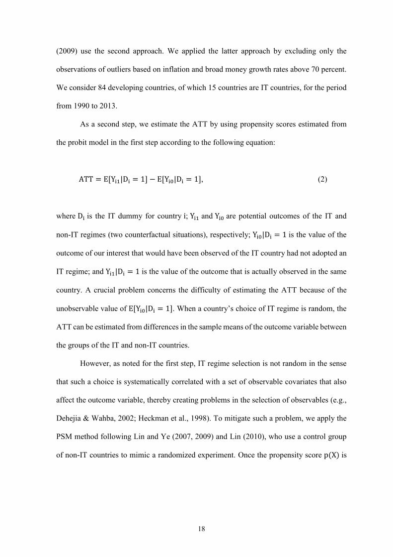
As a second step, we estimate the ATT by using propensity scores estimated from
the probit model in the first step according to the following equation:
ATT = E[Yi1|Di = 1] − E[Yi0|Di = 1], (2)
where Di is the IT dummy for country i; Yi1 and Yi0 are potential outcomes of the IT and
non-IT regimes (two counterfactual situations), respectively; Yi0|Di = 1 is the value of the
outcome of our interest that would have been observed of the IT country had not adopted an
IT regime; and Yi1|Di = 1 is the value of the outcome that is actually observed in the same
country. A crucial problem concerns the difficulty of estimating the ATT because of the
unobservable value of E[Yi0|Di = 1]. When a country’s choice of IT regime is random, the
ATT can be estimated from differences in the sample means of the outcome variable between
the groups of the IT and non-IT countries.
However, as noted for the first step, IT regime selection is not random in the sense
that such a choice is systematically correlated with a set of observable covariates that also
affect the outcome variable, thereby creating problems in the selection of observables (e.g.,
Dehejia & Wahba, 2002; Heckman et al., 1998). To mitigate such a problem, we apply the
PSM method following Lin and Ye (2007, 2009) and Lin (2010), who use a control group
of non-IT countries to mimic a randomized experiment. Once the propensity score p(X) is

19
given, the ATT is estimated under two main assumptions, i.e., conditional independence and
common support assumptions7, as follows:
ATT = E[Yi1|Di = 1, p(Xi)] − E[Yi0|Di = 0, p(Xi)] (3)
By utilizing the propensity scores estimated via the probit model, we apply four PSM
methods that are commonly used in the literature to estimate the ATT. The first matching
method is the nearest-neighbor matching without replacement, which matches each treated
observation to the n control observations that have the closest propensity scores, but each
control observation is used no more than one time as a match for a treated observation. We
use two nearest-neighbor matching estimators: n = 1 and n = 3 . The second method
involves radius matching, where each treated observation is matched with control
observations with estimated propensity scores that fall within a specified radius. We use two
radius matching estimators: r = 0.05 and r = 0.1 . The next method involves kernel
matching method, which matches each treated observation to control observations with
weights inversely proportional to the distance between the treated and control observations.
We use two kernel matching methods: Gaussian and Epanechnikov. The latter matching
7 The PSM method applied in this study is based on the method presented in Lin and Ye (2007, 2009). An initial assumption indicates that the assignment of treatments (IT regime selection) is independent of potential outcomes conditional on the observed covariates X, i.e., Y0, Y1 ⊥ D|X. As suggested by Lin and Ye (2007, 2009) and Rosenbaum and Rubin (1983), under the conditional independence assumption, the average treatment effect (ATE) is equal to the average treatment effect on the treated ( ATT), and ATT = E[Yi1|Di = 1] −
E[Yi0|Di = 1] is rewritten as ATT = E[Yi1|Di = 1, Xi] − E[Yi0|Di = 0, Xi]. Heckman et al. (1998) note that the ATT can be estimated consistently under a weaker independence assumption of E[Yi0|Di = 1, Xi] =
E[Yi0|Di = 0, Xi] , which requires that the outcomes of non-IT countries are independent of IT adoption decisions based on the observed covariates X. Such a weaker assumption generally yields different values of ATE and ATT . However, as the number of observed covariates increases, the ATT = E[Yi1|Di = 1, Xi] −
E[Yi0|Di = 0, Xi] equation becomes more difficult to estimate. To solve this high-dimensional set of observed covariates, Rosenbaum and Rubin (1983) recommend that treatment and control observations be matched based on propensity scores p(Xi), which are estimated from the probit model. The second assumption (0 <
p(Xi) < 1) suggests that every observation comes with a non-zero probability of IT regime adoption, which requires the presence of comparable control observations for each treated observation.
20
method involves applying the regression-adjusted local linear matching approach developed
by Heckman et al. (1998).
2.3.2 Empirical results
Our main interest is to determine how IT adoption affects income velocity variability in
developing countries. By definition, income velocity is composed of price levels, real
outputs, and broad money (or real output and real money balance). Thus, we attempt to
evaluate IT effects by estimating the treatment effect of an IT regime on the volatility of
income velocity as well as on the volatilities of its components to discuss sources of income
velocity variability. Similar to the works of Lin and Ye (2007, 2009), we measure the
volatilities of income velocity, inflation, output growth, broad money growth, and real
money balance growth as the standard deviation of variables over the previous seven years.8
Concerning the timing of IT adoption, we use two different IT adoption years as noted in the
previous subsection. We identify developing countries based on the IMF’s country
classification.9
2.3.2.1 Estimating propensity scores
The distribution of measured baseline covariates should be performed independent of the
treatment assignments conditional on the true propensity score. Thus, we should confirm
that our probit model is adequately specified by examining whether the distribution of
observed covariates is similar between the treated and control observations with the same
estimated propensity score. We conduct balancing tests that generally support the balancing
8 Our volatility measures are calculated by the standard deviation of the gap between the current variable and its seven-year moving average over the past seven years. 9 To ensure that the treatment and control groups are comparable, Lin and Ye (2009) and Lin (2010) exclude some non-IT countries with substantially different features (e.g., real GDP per capita) from IT countries. We also follow their method by constructing a different dataset by excluding some non-IT countries whose real GDP per capita levels are lower than those of the smallest IT country. The estimated results generally coincide with the results of the original dataset (see Table 2.8).
21
properties for our covariates.10 Once the probit model is specified, we first estimate the
propensity scores. As discussed in the previous subsection, we expect to find negative
coefficient signs for the one-year lagged inflation rate, broad money growth, trade openness,
fixed exchange rate regime, and fiscal balance and positive coefficient signs for the real per
capita GDP growth rate and financial openness.
Table 2.3 presents the estimation results of the probit model for the loose IT and strict
IT regimes.11 Most estimates are generally consistent with our expected signs except for the
coefficient on broad money growth, which shows insignificant results. The estimation results
indicate that countries with higher inflation rates for the previous period, sound fiscal
conditions, higher levels of trade openness, and a fixed exchange rate regime are less likely
to adopt an IT regime. In addition, countries with higher GDP per capita growth and more
financial openness are more likely to adopt an IT regime. These results generally coincide
with the findings of previous studies (e.g., de Mendonca & de Guimaraes e Souza, 2012; Lin
& Ye, 2007).
10 Once the balancing condition (D ⊥ X|p(X)) is satisfied, a conclusion can be made as to whether the treatment and control groups with similar propensity scores follow the similar distribution of observed characteristics (covariates) independent of the treatment status. Tables 2.9 and 2.10 present the mean values of the covariates of the treatment and control groups and the p-value of a balancing test for the loose and strict IT regimes, respectively. We report three balancing tests for income velocity volatility (the test results for other outcome variables are available on request). The null hypothesis of the balancing test is that the mean values of the covariates are similar for both the treatment and control groups. For the balancing tests of the strict IT regime, the mean values of all variables of both the IT and non-IT countries after matching become similar with the evidence that the p-values fail to reject the null hypothesis. However, the balancing test results for the loose IT regime are less convincing for some covariates. The null of identical means is rejected at the 1 percent significance level for financial openness under the nearest-neighbor matching condition (p-value of 0.09) as well as under lagged inflation and GDP per capita growth based on radius (p-values of 0.06 and 0.04) and kernel matching (p-values of 0.07 and 0.05). Thus, matching generally helps reduce the bias in distributions of observables for the IT and non-IT country groups. 11 For the robustness checks of our empirical results, we follow the work of Lin and Ye (2009) and examine whether the results are sensitive to alternative specifications of the probit model by adding government debt to GDP ratio and the turnover rate of central bank governors, which are obtained from Ali Abbas et al. (2010) and Cukierman et al. (1992), respectively. The turnover index was supplemented with data from Crowe and Meade (2007) and Dreher et al. (2008). In addition, we also check whether our results are robust to different sample periods by estimating the original probit model over the alternative sample period from 1990 to 2007. These robustness checks do not undermine our results (see the estimated results of the probit models and the ATTs in Tables 2.11 and 2.12, respectively).
22
2.3.2.2 Average treatment effects
Once the propensity scores are estimated, we estimate the ATT by applying matching
methods. We first attempt to ensure the sharing of the same support or to confirm the highly
and reasonably comparability between the treatment and control groups. As in the works of
Lin and Ye (2007, 2009) and Thornton and Vasilakis (2017), we reconstruct the dataset that
satisfies the common support assumption by sorting all observations based on estimated
propensity scores and discarding control units with propensity scores that fall below the
lowest treatment unit value and exceed the highest treatment unit value. Table 4 reports the
matching results for the loose and strict IT regimes based on the modified samples. The first
seven columns of Table 2.4 report the results of the loose IT regime, and the last seven
columns show the results of the strict IT regime. We present the estimated ATTs of the seven
types of matching methods with analytical standard errors and bootstrapped standard errors.
Many studies have generally highlighted the effectiveness of IT regimes in terms of inflation
levels in developing countries, whereas other studies, such as Thornton (2016), doubt their
effectiveness. The first row of Table 4 highlights the important role of an IT regime in
reducing the inflation level, although less clear negative effects are observed under a loose
IT regime. This result is consistent with the findings of Samarina et al. (2014), Lin and Ye
(2009) and de Mendonca and de Guimaraes e Souza (2012) on the IT effects in developing
countries.
The main concern in this study is on the variabilities of income velocity and its
components as the outcome variables, which allows us to discuss the role of stable income
velocities in the monetary policy frameworks of developing countries. The second row of
Table 4 shows the ATT results of the IT regime in terms of income velocity volatility, and
the last four rows present the ATT estimates of the IT regime for volatilities in inflation,
output growth, money growth, and real money balance growth. The estimated results show
23
that income velocity volatility is negatively significant irrespective of the choice of the IT
regime, which indicates that IT adoption helps stabilize income velocity in developing
countries. In addition, the results clearly show that IT adoption reduces volatilities of
inflation and output growth in loose and strict IT regimes. Moreover, IT adoption reduces
volatilities of money growth and real money balance growth in a loose IT regime, whereas
the estimated ATTs are negative, although insignificant for a strict IT regime. The
decomposition analysis generally shows that a reduction in income velocity volatility
originates from all of its components (inflation, real output growth, money growth, and real
money balance growth), although less clear results on money growth and real money balance
growth in the case of a strict IT regime. Our results on the role of IT policies in stabilizing
income velocity variability in developing countries stands in sharp contrast with the findings
of Lin and Ye (2007), who showed an insignificant link between IT adoption and income
velocity volatility in advanced countries.
Historically, as a solution after the collapse of the Bretton Woods system in the mid-
1970s, many countries initiated a monetary targeting framework. Inspired by monetarists’
quantity theory of money, central banks, mainly those in advanced countries, started to apply
monetary aggregates as intermediate targets through their monetary policy conduct (Argy et
al., 1990; Mishkin, 2006; Woodford, 2008). During this period, the success of monetary
targeting required the presence of a strong relationship between targeted monetary
aggregates and inflation and/or nominal income, i.e., income velocity, along with stability
in money demand (Estrella & Mishkin, 1997; Mishkin, 2006). An early study by Ritter
(1959) also stresses that income velocity instability generates ineffective monetary policies.
However, many countries experienced periods of volatile income velocity with the unstable
money demand in the 1980s, thereby inducing the breakdown of monetarism and monetary
targeting (Lin & Ye, 2007). Roger (2009) notes that many advanced countries started to
24
abandon monetary targeting in the 1980s and all advanced countries had abandoned it by the
late 1990s.
However, developing economies adopted monetary targeting in the 1980s and 1990s,
and some are still pursuing this monetary framework. According to historical arguments on
monetary frameworks, stable income velocity is central to successful monetary targeting in
developing economies. Early studies, such as Park (1970) and Melitz and Correa (1970),
show international variations in income velocity, with Park (1970) finding that less-
developed countries are generally characterized by higher levels of income velocity
variability than advanced countries because of their unstable economic, social, and political
systems; volatile inflation patterns; and the large degree of monetization (see, e.g., Driscoll
& Lahiri, 1983; Chowdhury, 1994; Owoye, 1997). Owoye (1997) investigates sources of
income velocity volatility in less-developed countries and shows that income velocity
volatility is mainly a result of money growth in most sampled countries, and fluctuations of
real output and inflation rates are also central in determining income velocity volatility
depending on sampled countries. As the IT regime has recently become more popular, some
developing countries have also adopted it as a monetary policy framework. With the
importance of stable income velocity and the current trend of the adoption of an IT regime,
one crucial question concerns whether an IT regime can help stabilize income velocity in
developing economies. If so, then monetary targeting can serve as a reliable framework. Our
estimation results support the effectiveness of an IT regime in decreasing income velocity
variability and could provide monetary authorities in developing countries with the
justification of the control of monetary aggregates as an effective policy measure applied
under an IT regime.
More importantly, our analysis results can also be linked to Taylor’s (2000) argument
for policy consistency. Recent discussions on IT in emerging economies suggest that an IT
25
regime serves as an alternative to monetary aggregate targeting. However, Taylor (2000)
argues that there is no inconsistency between IT and monetary aggregates as an instrument
of policy rule and suggests that an IT regime does not serve as an alternative to policies that
focus on monetary aggregates. Taylor (2000) also describes a policy rule for achieving
targets under an IT regime. As a policy rule, an instrument can involve a short-term overnight
interest rate, although monetary bases or other monetary aggregates can also be used as
instruments. As noted by Poole (1970), the choice of a policy rule between interest rates and
monetary bases (or other monetary aggregates) as instruments is essential. Monetary
aggregates would be the preferred instrument when considerable uncertainty is involved in
measuring real interest rates or when relatively significant shocks to investment or net
exports occur. Moreover, when income velocity is relatively stable, monetary aggregates
would be the better instrument. Taylor (2000) stresses that the preference for the interest rate
as the instrument primarily reflects income velocity uncertainty, but developing economies
often face the circumstances where real interest rate is difficult to measure and the overnight
nominal interest rate is not a good policy measure. 12 In addition, developing countries
experience several institutional constraints on monetary policy conduct (e.g., the
underdevelopment of money and financial markets with strict financial regulations). Thus,
monetary authorities in developing economies might prefer or rely on monetary policy rules
with monetary aggregates to achieve inflation targets, particularly under conditions of stable
income velocity. Our results showing the IT effects on income velocity provide empirical
support for Taylor’s (2000) suggestion that monetary aggregates will be the appropriate
instrument under an IT regime.
12 Taylor (2000) notes that such circumstances may be present in emerging countries. In a high inflation period, measuring the real interest rate and risk premiums is difficult. In a high growth period, determining and measuring the equilibrium real interest rate is also difficult.
26
Concerning the sources of the IT role in reducing income velocity variability, our
estimation results generally show that IT adoption would reduce volatilities of inflation and
real output growth irrespective of the choice of the loose or strict IT regimes. This finding
implies that an IT regime contributes to price stability as well as macroeconomic stability in
developing countries. In addition, the estimation results suggest that an IT regime also helps
stabilize volatilities of money growth and real money balance growth, i.e., the stability of
money demand, in developing countries, although the results of a strict IT regime show less
clear evidence. Based on our results showing favorable IT effects on income velocity
variability, the findings of the decomposition analysis are generally consistent with the
results of Owoye (1997), who shows that volatility in income velocity is related to money
growth, inflation, and real outputs. In addition, our decomposition analysis supports the
notion that IT adoption offers substantial economic benefits of macroeconomic stabilization
by securing real outputs and inflation stability. Moreover, our results on IT effects suggest
that IT adoption enables developing countries to satisfy crucial conditions necessary to
support the effective role of monetary aggregates, which require the presence of income
velocity stability as well as money demand stability as argued by Estrella and Mishkin
(1997) and Mishkin (2006).
2.3.3 Heterogeneity in treatment effects
Substantial heterogeneity social and economic development is known to occur in developing
countries. Many studies have shown that the causes and consequences of IT adoption can be
associated with various economic and institutional characteristics of developing countries
(e.g., Carare & Stone, 2006; Fraga et al., 2003; Fry et al., 2000; Masson et al., 1997; Minella
et al., 2003; Mishkin, 2004; Mishkin & Savastano, 2001; Svensson, 2002; Lin & Ye, 2009).
Thus, examining the heterogeneous effects of IT adoption on income velocity variability is
critical for conducting policy evaluations of developing countries. Lin and Ye (2009) analyze

27
the crucial heterogeneities of average treatment effects of IT adoption on inflation and its
variability, and our study also evaluates four possible sources of heterogeneity following Lin
and Ye (2009). As a first possible source, IT effects can depend on whether a country
satisfies the precondition of IT adoption, which is captured by the estimated propensity score.
The second source concerns time lagged effects of IT adoption based on the argument that
it often takes some time for monetary policy to be effective. The third and fourth sources
concern the roles of fiscal conditions and exchange rate arrangements in determining the
effects of IT adoption, respectively. Mishkin (2004) and Mishkin and Savastano (2001) note
that the performance of an IT regime would be influenced by government fiscal positions
and levels of exchange rate flexibility.
Table 2.5 presents the estimated results of the four sources of heterogeneous effects
of loose and strict IT regimes on our outcome variable of income velocity volatility. The
first column shows the results of the OLS regression of income velocity volatility on the IT
regime, which presents the consistent finding of the negative coefficient with the matching
analysis of the previous subsection. In the second column, we include the estimated
propensity score and interaction term of the IT regime and the difference between the
estimated propensity score and its sample mean to evaluate how IT effects are dependent on
the precondition of IT adoption. The results show that coefficients on the IT dummy are
negative for the loose and strict IT regimes, whereas those on the interaction term are
negative, although less significant for the strict IT regime. These results imply that the
treatment effect of the IT regime for the mean of the propensity score is significantly
negative with the estimated coefficients of −0.07 and −0.06 for the loose and strict IT
regimes, respectively. More importantly, the coefficient on the interaction term highlights
the presence of heterogeneity. The negative coefficient suggests that the effectiveness of an
IT regime is more apparent for countries with high estimated propensity scores that reflect
28
more favorable preconditions for IT adoption. IT would lead to an additional reduction in
income velocity volatility (standard deviation) of 0.03 points for every 10 percent increase
in the propensity score.
To examine the role of the time length on IT effects, the third column includes the
interaction term of the IT dummy and the time length (year) from IT adoption.13 The results
show that the coefficient on the interaction term is significantly negative for the loose IT
regime, and it is negative but less significant for the strict IT regime. The effectiveness of
the IT regime is dependent on the time length since the IT adoption; therefore, IT is likely
to become effective at reducing income velocity variability over time. In addition, we test
the role of exchange rate arrangements in heterogeneous IT effects by including a fixed
exchange rate dummy and an interaction term for the IT dummy and a fixed exchange rate
dummy in the model. The estimation results shown in the fourth column illustrate that the
coefficient on the interaction term is significantly positive irrespective of whether loose or
strict IT regimes are involved. The treatment effect on income velocity volatility would be
zero when a country adopts a fixed exchange rate regime. IT reduces income velocity
volatility under a flexible exchange rate regime, but it fails to influence volatility under a
fixed exchange rate regime. An IT regime would be effective in reducing income velocity
volatility only under a floating exchange rate regime. Moreover, we examine the role of a
fiscal disciple by incorporating fiscal balance and its interaction term with the IT dummy.
The fifth column shows that the coefficient on the interaction term is insignificant for the
loose and strict IT regimes; thus, no evidence is observed for the heterogeneous effects on
IT regime performance.
13 As in Lin and Ye (2009), this study does not include the time length variable in the regression because the value of the time length variable is the same as the interaction term of the IT dummy and time length.

29
2.3.4 Alternative method
In addition to the PSM method, we also apply the DID method as an alternative approach.
The PSM method can serve as an appropriate method of addressing selection biases in
observed covariates in the adoption of an IT regime. However, as noted in the literature (e.g.,
Pearl, 2000), the PSM method is limited because it controls only for observed covariates and
unobserved covariates or factors may induce hidden bias. In addition, the PSM method
requires the use of large samples with substantial common regions of treatment and control
groups. The DID method can properly address selection biases originating from time-
invariant unobserved characteristics by differentiating between the pre-period and post-
period, and it can also be used to estimate treatment effects by comparing pre- and post-
treatment differences from the outcomes of treatment and control groups.
The main assumption of the DID method is that the outcomes of treatment and
control groups would follow the same time trends in the absence of treatment. When the
parallel trend assumption holds and we can credibly rule out the presence of any other time-
variant changes that may confound the treatment, the DID method is a trustworthy approach
to apply. However, a crucial methodological problem related to the DID method identified
in our study concerns the identification of adoption dates for non-IT countries that have
never adopted an IT regime. Another problem may be related to potential violations of the
parallel time trend condition because the timing of IT adoption varies across IT countries.
Although the DID method can suffer from such issues, we attempt to ascertain the empirical
validity of our baseline results derived from the matching analysis. The DID approach is
widely used in the IT-related literature (e.g., Ball & Sheridan, 2005; Batini & Laxton, 2007;
Goncalves & Salles, 2008; Thornton, 2016; Samarina et al., 2014). Following previous work,
we apply the DID method as follows:
Xi,post − Xi,pre = β0 + β1Xi,pre + β2ITi + εi, (4)
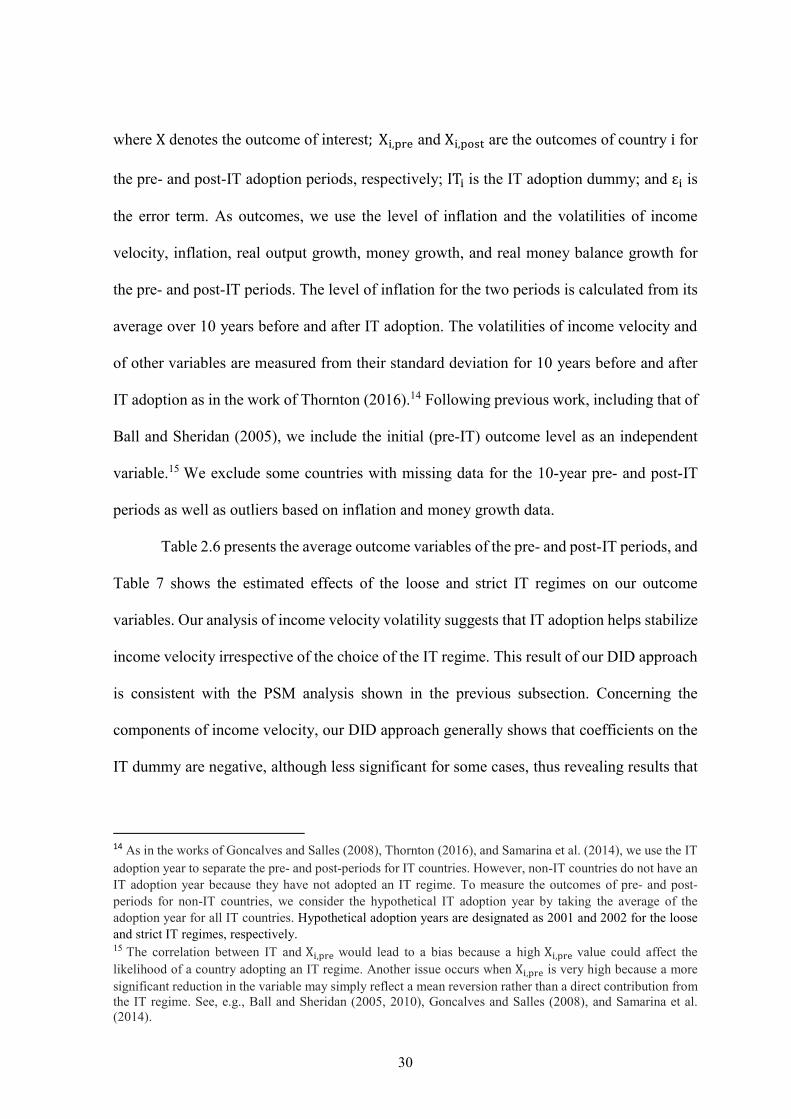
30
where X denotes the outcome of interest; Xi,pre and Xi,post are the outcomes of country i for
the pre- and post-IT adoption periods, respectively; ITi is the IT adoption dummy; and εi is
the error term. As outcomes, we use the level of inflation and the volatilities of income
velocity, inflation, real output growth, money growth, and real money balance growth for
the pre- and post-IT periods. The level of inflation for the two periods is calculated from its
average over 10 years before and after IT adoption. The volatilities of income velocity and
of other variables are measured from their standard deviation for 10 years before and after
IT adoption as in the work of Thornton (2016).14 Following previous work, including that of
Ball and Sheridan (2005), we include the initial (pre-IT) outcome level as an independent
variable.15 We exclude some countries with missing data for the 10-year pre- and post-IT
periods as well as outliers based on inflation and money growth data.
Table 2.6 presents the average outcome variables of the pre- and post-IT periods, and
Table 7 shows the estimated effects of the loose and strict IT regimes on our outcome
variables. Our analysis of income velocity volatility suggests that IT adoption helps stabilize
income velocity irrespective of the choice of the IT regime. This result of our DID approach
is consistent with the PSM analysis shown in the previous subsection. Concerning the
components of income velocity, our DID approach generally shows that coefficients on the
IT dummy are negative, although less significant for some cases, thus revealing results that
14 As in the works of Goncalves and Salles (2008), Thornton (2016), and Samarina et al. (2014), we use the IT adoption year to separate the pre- and post-periods for IT countries. However, non-IT countries do not have an IT adoption year because they have not adopted an IT regime. To measure the outcomes of pre- and post-periods for non-IT countries, we consider the hypothetical IT adoption year by taking the average of the adoption year for all IT countries. Hypothetical adoption years are designated as 2001 and 2002 for the loose and strict IT regimes, respectively. 15 The correlation between IT and Xi,pre would lead to a bias because a high Xi,pre value could affect the likelihood of a country adopting an IT regime. Another issue occurs when Xi,pre is very high because a more significant reduction in the variable may simply reflect a mean reversion rather than a direct contribution from the IT regime. See, e.g., Ball and Sheridan (2005, 2010), Goncalves and Salles (2008), and Samarina et al. (2014).
31
are consistent with the findings of the PSM method. Thus, our PSM results are robust, and
an IT regime would generally reduce the volatilities of each component of income velocity.
2.4 Conclusion
This study has applied the PSM method to examine whether IT helps stabilize income
velocity variability. The PSM method has commonly been used to eliminate self-selection
bias, although it may suffer from issues related to small samples as well as hidden biases
derived from unobserved covariates or factors (Pearl, 2000). Thus, to confirm the empirical
validity of our PSM results, this study has also applied another method widely used in IT-
related studies, the DID method. The empirical results of both methods have indicated that
IT would help stabilize income velocity in developing countries. Thus, our findings have
shown clear support for Taylor’s (2000) argument that monetary authorities in developing
economies would prefer using monetary policy rule with monetary aggregates to achieve
inflation targets under stable income velocity. In addition, our empirical results regarding IT
effects on income velocity have highlighted that monetary authorities can pursue monetary
aggregates as an effective policy measure under an IT regime. Moreover, our decomposition
analysis of income velocity variability has provided evidences that IT lessens volatilities of
inflation, real output growth, and money growth. Furthermore, our analysis of heterogeneous
effects has revealed that an IT regime would be effective in reducing income velocity
volatility under the favorable preconditions of IT adoption and floating exchange rate regime
application. The time length also influences the effectiveness of an IT regime, and IT is
likely to become more effective in lowering income velocity volatility over time.
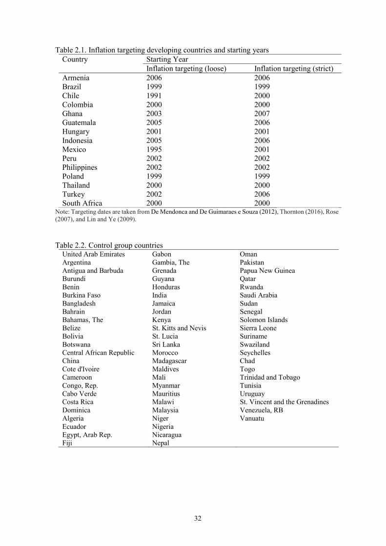
32
Table 2.1. Inflation targeting developing countries and starting years Country Starting Year Inflation targeting (loose) Inflation targeting (strict) Armenia 2006 2006 Brazil 1999 1999 Chile 1991 2000 Colombia 2000 2000 Ghana 2003 2007 Guatemala 2005 2006 Hungary 2001 2001 Indonesia 2005 2006 Mexico 1995 2001 Peru 2002 2002 Philippines 2002 2002 Poland 1999 1999 Thailand 2000 2000 Turkey 2002 2006 South Africa 2000 2000
Note: Targeting dates are taken from De Mendonca and De Guimaraes e Souza (2012), Thornton (2016), Rose (2007), and Lin and Ye (2009). Table 2.2. Control group countries
United Arab Emirates Gabon Oman Argentina Gambia, The Pakistan Antigua and Barbuda Grenada Papua New Guinea Burundi Guyana Qatar Benin Honduras Rwanda Burkina Faso India Saudi Arabia Bangladesh Jamaica Sudan Bahrain Jordan Senegal Bahamas, The Kenya Solomon Islands Belize St. Kitts and Nevis Sierra Leone Bolivia St. Lucia Suriname Botswana Sri Lanka Swaziland Central African Republic Morocco Seychelles China Madagascar Chad Cote d'Ivoire Maldives Togo Cameroon Mali Trinidad and Tobago Congo, Rep. Myanmar Tunisia Cabo Verde Mauritius Uruguay Costa Rica Malawi St. Vincent and the Grenadines Dominica Malaysia Venezuela, RB Algeria Niger Vanuatu Ecuador Nigeria Egypt, Arab Rep. Nicaragua Fiji Nepal
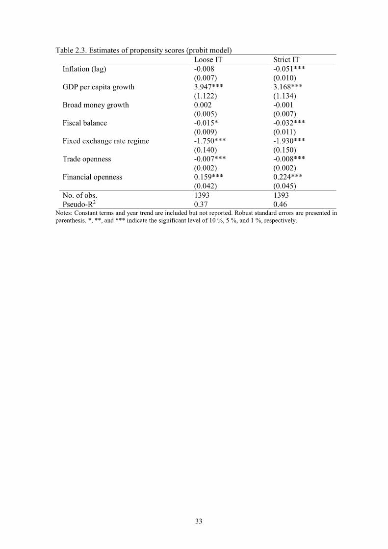
33
Table 2.3. Estimates of propensity scores (probit model) Loose IT Strict IT Inflation (lag) -0.008
(0.007) -0.051*** (0.010)
GDP per capita growth 3.947*** (1.122)
3.168*** (1.134)
Broad money growth 0.002 (0.005)
-0.001 (0.007)
Fiscal balance -0.015* (0.009)
-0.032*** (0.011)
Fixed exchange rate regime -1.750*** (0.140)
-1.930*** (0.150)
Trade openness -0.007*** (0.002)
-0.008*** (0.002)
Financial openness 0.159*** (0.042)
0.224*** (0.045)
No. of obs. 1393 1393 Pseudo-R2 0.37 0.46
Notes: Constant terms and year trend are included but not reported. Robust standard errors are presented in parenthesis. *, **, and *** indicate the significant level of 10 %, 5 %, and 1 %, respectively.
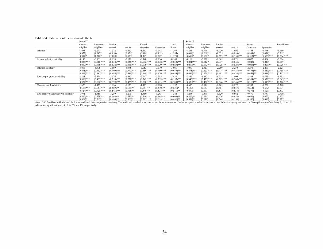
34
Table 2.4. Estimates of the treatment effects
Loose IT Strict IT Nearest-
neighbor 3-nearest-neighbor
Radius Kernel Local linear
Nearest-neighbor
3-nearest-neighbor
Radius Kernel Local linear r=0.05 r=0.10 Gaussian Epanechn r=0.05 r=0.10 Gaussian Epanechn Inflation -1.498
(0.972) [0.907]*
-2.271 (1.282)* [1.316]*
-1.372 (0.950) [1.089]
-1.412 (0.926) [1.053]
-1.392 (0.919) [1.107]
-1.342 (0.952) [1.082]
-1.363 (1.395) [1.125]
-1.283 (0.684)* [0.689]*
-1.996 (1.069)* [0.806]*
-1.720 (1.035)* [0.573]***
-1.692 (0.989)* [0.553]***
-1.745 (0.984)* [0.513]***
-1.748 (1.038)* [0.555]***
-1.650 (0.261) [0.534]***
Income velocity volatility -0.193 (0.034)*** [0.032]***
-0.151 (0.040)*** [0.038]***
-0.135 (0.038)*** [0.028]***
-0.137 (0.036)*** [0.031]***
-0.140 (0.036)*** [0.030]***
-0.136 (0.038)*** [0.029]***
-0.140 (0.053)*** [0.029]***
-0.118 (0.031)*** [0.030]**
-0.070 (0.042)* [0.032]**
-0.065 (0.047) [0.028]**
-0.071 (0.045) [0.027]***
-0.072 (0.045) [0.028]***
-0.064 (0.047) [0.029]**
-0.064 (0.049) [0.025]**
Inflation volatility -3.013 (0.478)*** [0.503]***
-3.396 (0.542)*** [0.585]***
-3.069 (0.400)*** [0.495]***
-3.075 (0.390)*** [0.481]***
-3.053 (0.386)*** [0.449]***
-3.070 (0.400)*** [0.476]***
-3.081 (0.685)*** [0.484]***
-3.050 (0.478)*** [0.485]***
-2.317 (0.623)*** [0.629]***
-2.289 (0.478)*** [0.491]***
-2.250 (0.457)*** [0.438]***
-2.276 (0.455)*** [0.445]***
-2.299 (0.480)*** [0.484]***
-2.221 (0.758)*** [0.452]***
Real output growth volatility -2.228 (0.360)*** [0.374]***
-2.574 (0.403)*** [0.506]***
-2.374 (0.258)*** [0.399]***
-2.452 (0.251)*** [0.425]***
-2.447 (0.249)*** [0.398]***
-2.383 (0.259)*** [0.413]***
-2.430 (0.557)*** [0.388]***
-1.836 (0.346)*** [0.378]***
-1.645 (0.475)*** [0.430]***
-1.758 (0.319)*** [0.346]***
-1.800 (0.305)*** [0.346]***
-1.803 (0.304)*** [0.316]***
-1.753 (0.320)*** [0.343]***
-1.735 (0.645)*** [0.316]***
Money growth volatility -1.626 (0.513)*** [0.524]***
-1.429 (0.547)*** [0.620]***
-1.116 (0.569)** [0.543]***
-1.173 (0.558)** [0.515]**
-1.177 (0.554)** [0.546]**
-1.120 (0.570)** [0.524]**
-1.152 (0.631)* [0.511]**
-0.635 (0.509) [0.499]
-0.114 (0.633) [0.637]
-0.265 (0.681) [0.577]
-0.272 (0.657) [0.534]
-0.293 (0.654) [0.573]
-0.259 (0.682) [0.620]
-0.340 (0.774) [0.573]
Real money balance growth volatility -1.971 (0.527)*** [0.528]***
-1.359 (0.578)** [0.562]**
-1.259 (0.564)** [0.496]**
-1.291 (0.553)** [0.500]***
-1.310 (0.549)** [0.503]***
-1.263 (0.565)** [0.518]**
-1.344 (0.603)** [0.492]***
-1.248 (0.529)** [0.554]**
-0.370 (0.634) [0.638]
-0.620 (0.676) [0.564]
-0.662 (0.653) [0.554]
-0.670 (0.651) [0.540]
-0.587 (0.677) [0.610]
-0.709 (0.773) [0.533]
Notes: 0.06 fixed bandwidth is used for kernel and local linear regression matching. The analytical standard errors are shown in parentheses and the bootstrapped standard errors are shown in brackets (they are based on 500 replications of the data). *, ** and *** indicate the significant level of 10 %, 5% and 1%, respectively.
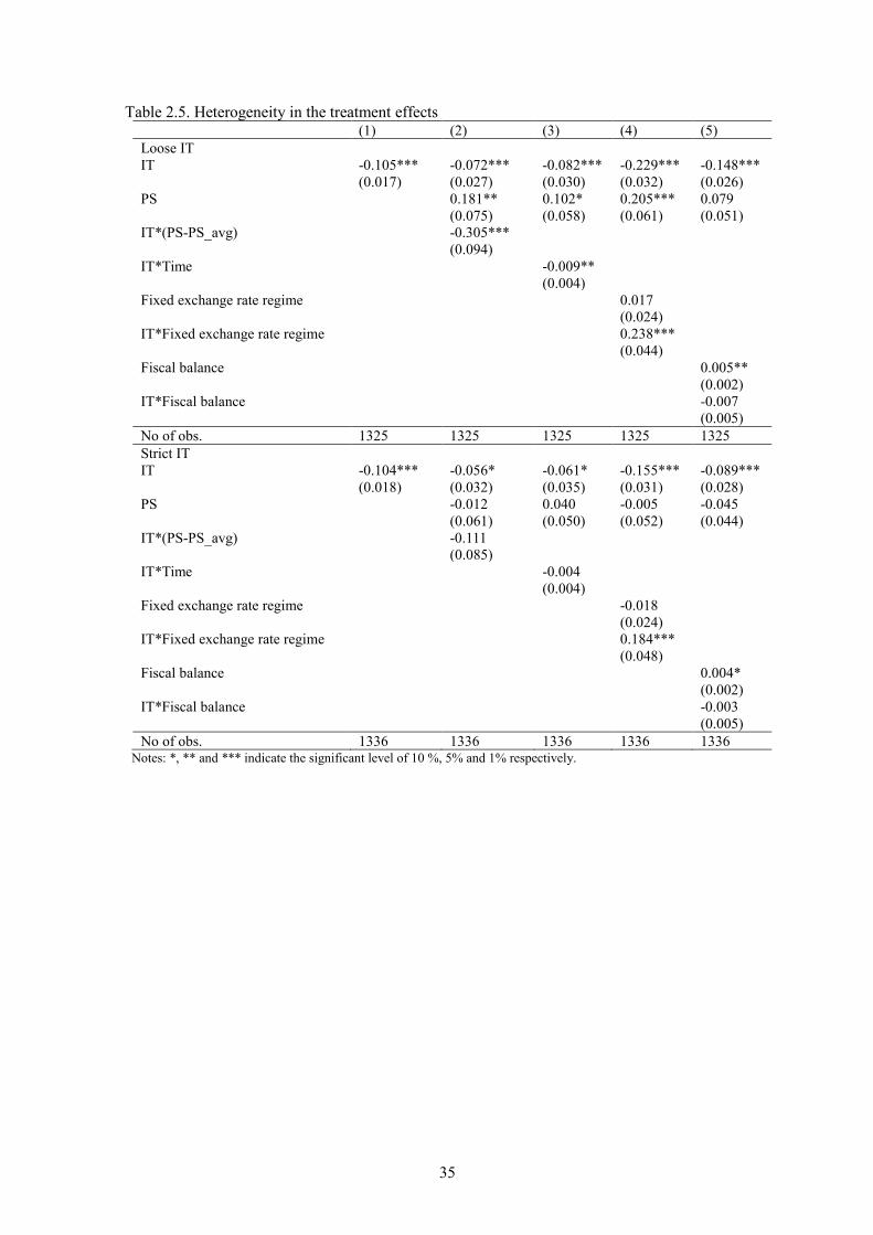
35
Table 2.5. Heterogeneity in the treatment effects (1) (2) (3) (4) (5) Loose IT IT -0.105***
(0.017) -0.072*** (0.027)
-0.082*** (0.030)
-0.229*** (0.032)
-0.148*** (0.026)
PS 0.181** (0.075)
0.102* (0.058)
0.205*** (0.061)
0.079 (0.051)
IT*(PS-PS_avg) -0.305*** (0.094)
IT*Time -0.009** (0.004)
Fixed exchange rate regime 0.017 (0.024)
IT*Fixed exchange rate regime 0.238*** (0.044)
Fiscal balance 0.005** (0.002)
IT*Fiscal balance -0.007 (0.005)
No of obs. 1325 1325 1325 1325 1325 Strict IT IT -0.104***
(0.018) -0.056* (0.032)
-0.061* (0.035)
-0.155*** (0.031)
-0.089*** (0.028)
PS -0.012 (0.061)
0.040 (0.050)
-0.005 (0.052)
-0.045 (0.044)
IT*(PS-PS_avg) -0.111 (0.085)
IT*Time -0.004 (0.004)
Fixed exchange rate regime -0.018 (0.024)
IT*Fixed exchange rate regime 0.184*** (0.048)
Fiscal balance 0.004* (0.002)
IT*Fiscal balance -0.003 (0.005)
No of obs. 1336 1336 1336 1336 1336 Notes: *, ** and *** indicate the significant level of 10 %, 5% and 1% respectively.
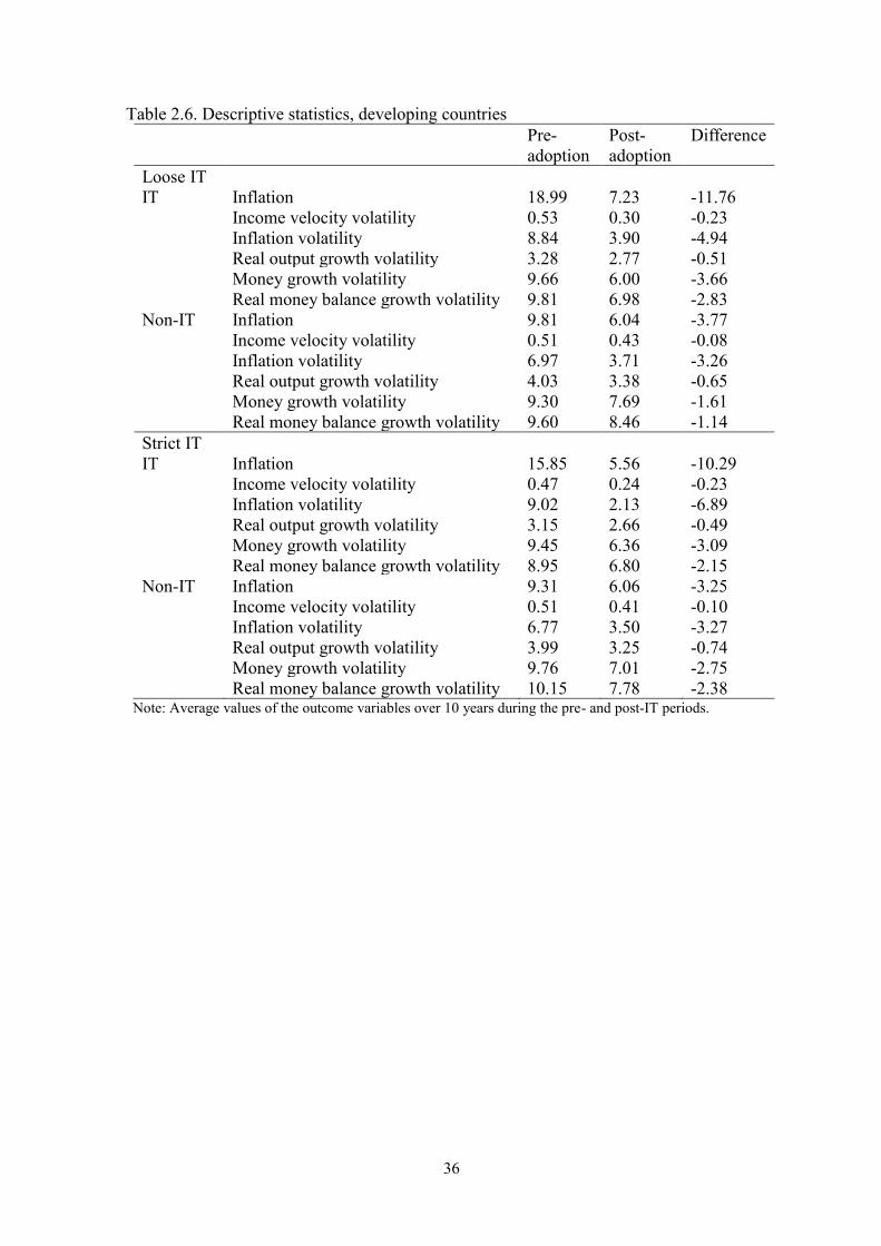
36
Table 2.6. Descriptive statistics, developing countries Pre-
adoption Post-adoption
Difference
Loose IT IT Inflation 18.99 7.23 -11.76 Income velocity volatility 0.53 0.30 -0.23 Inflation volatility 8.84 3.90 -4.94 Real output growth volatility 3.28 2.77 -0.51 Money growth volatility 9.66 6.00 -3.66 Real money balance growth volatility 9.81 6.98 -2.83 Non-IT Inflation 9.81 6.04 -3.77 Income velocity volatility 0.51 0.43 -0.08 Inflation volatility 6.97 3.71 -3.26 Real output growth volatility 4.03 3.38 -0.65 Money growth volatility 9.30 7.69 -1.61 Real money balance growth volatility 9.60 8.46 -1.14 Strict IT IT Inflation 15.85 5.56 -10.29 Income velocity volatility 0.47 0.24 -0.23 Inflation volatility 9.02 2.13 -6.89 Real output growth volatility 3.15 2.66 -0.49 Money growth volatility 9.45 6.36 -3.09 Real money balance growth volatility 8.95 6.80 -2.15 Non-IT Inflation 9.31 6.06 -3.25 Income velocity volatility 0.51 0.41 -0.10 Inflation volatility 6.77 3.50 -3.27 Real output growth volatility 3.99 3.25 -0.74 Money growth volatility 9.76 7.01 -2.75 Real money balance growth volatility 10.15 7.78 -2.38
Note: Average values of the outcome variables over 10 years during the pre- and post-IT periods.
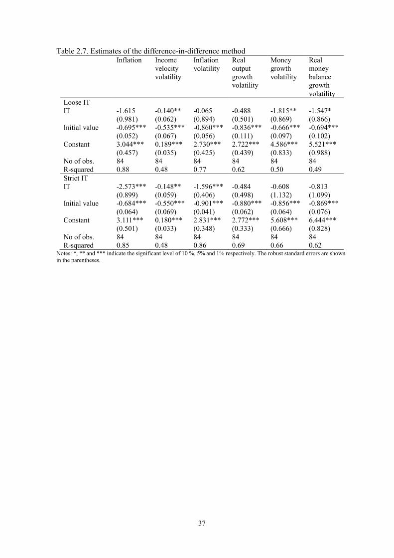
37
Table 2.7. Estimates of the difference-in-difference method Inflation Income
velocity volatility
Inflation volatility
Real output growth volatility
Money growth volatility
Real money balance growth volatility
Loose IT IT -1.615
(0.981) -0.140** (0.062)
-0.065 (0.894)
-0.488 (0.501)
-1.815** (0.869)
-1.547* (0.866)
Initial value -0.695*** (0.052)
-0.535*** (0.067)
-0.860*** (0.056)
-0.836*** (0.111)
-0.666*** (0.097)
-0.694*** (0.102)
Constant 3.044*** (0.457)
0.189*** (0.035)
2.730*** (0.425)
2.722*** (0.439)
4.586*** (0.833)
5.521*** (0.988)
No of obs. 84 84 84 84 84 84 R-squared 0.88 0.48 0.77 0.62 0.50 0.49 Strict IT IT -2.573***
(0.899) -0.148** (0.059)
-1.596*** (0.406)
-0.484 (0.498)
-0.608 (1.132)
-0.813 (1.099)
Initial value -0.684*** (0.064)
-0.550*** (0.069)
-0.901*** (0.041)
-0.880*** (0.062)
-0.856*** (0.064)
-0.869*** (0.076)
Constant 3.111*** (0.501)
0.180*** (0.033)
2.831*** (0.348)
2.772*** (0.333)
5.608*** (0.666)
6.444*** (0.828)
No of obs. 84 84 84 84 84 84 R-squared 0.85 0.48 0.86 0.69 0.66 0.62
Notes: *, ** and *** indicate the significant level of 10 %, 5% and 1% respectively. The robust standard errors are shown in the parentheses.
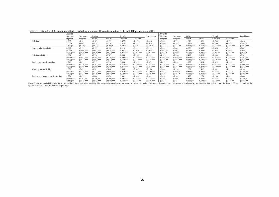
38
Table 2.8: Estimates of the treatment effects (excluding some non-IT countries in terms of real GDP per capita in 2013)
Loose IT Strict IT Nearest-
neighbor 3-nearest-neighbor
Radius Kernel Local linear Nearest-neighbor
3-nearest-neighbor
Radius Kernel Local linear r=0.05 r=0.10 Gaussian Epanechn r=0.05 r=0.10 Gaussian Epanechn Inflation -1.985
(1.002)** [1.137]*
-1.581 (1.607) [1.118]
-1.187 (1.418) [0.822]
-1.533 (1.336) [0.789]*
-1.477 (1.318) [0.803]*
-1.272 (1.413) [0.805]
-1.496 (1.649) [0.796]*
-0.861 (0.660) [0.721]
-1.713 (1.149) [0.772]**
-1.698 (1.446) [0.575]***
-1.621 (1.408) [0.554]***
-1.700 (1.400)** [0.567]***
-1.718 (1.446) [0.597]***
-1.610 (0.948)* [0.567]***
Income velocity volatility -0.092 (0.029)*** [0.030]***
-0.135 (0.046)*** [0.039]***
-0.115 (0.041)*** [0.036]***
-0.116 (0.038)*** [0.031]***
-0.114 (0.037)*** [0.033]***
-0.121 (0.040)*** [0.034]***
-0.118 (0.055)** [0.036]***
-0.061 (0.031)** [0.033]*
-0.043 (0.048) [0.029]
-0.056 (0.044) [0.028]**
-0.057 (0.043) [0.026]**
-0.056 (0.043) [0.025]**
-0.055 (0.044) [0.025]**
-0.047 (0.049) [0.025]*
Inflation volatility -1.634 (0.421)*** [0.472]***
-2.932 (0.687)*** [0.674]***
-2.936 (0.548)*** [0.582]***
-2.907 (0.514)*** [0.577]***
-2.908 (0.506)*** [0.570]***
-2.988 (0.546)*** [0.559]***
-2.921 (0.818)*** [0.587]***
-1.187 (0.401)*** [0.486]**
-2.226 (0.689)*** [0.687]***
-2.417 (0.594)*** [0.648]***
-2.313 (0.577)*** [0.593]***
-2.304 (0.574)*** [0.603]***
-2.406 (0.596)*** [0.614]***
-2.149 (0.847)** [0.627]***
Real output growth volatility -1.248 (0.213)*** [0.233]***
-1.835 (0.326)*** [0.268]***
-1.913 (0.297)*** [0.268]***
-1.956 (0.280)*** [0.249]***
-1.930 (0.276)*** [0.253]***
-1.915 (0.296)*** [0.253]***
-1.872 (0.381)*** [0.252]***
-1.419 (0.219)*** [0.226]***
-1.854 (0.322)*** [0.364]***
-1.855 (0.327)*** [0.289]***
-1.814 (0.318)*** [0.230]***
-1.813 (0.317)*** [0.309]***
-1.856 (0.328)*** [0.307]***
-1.731 (0.406)*** [0.313]***
Money growth volatility -1.058 (0.477)** [0.497]**
-2.021 (0.718)*** [0.731]***
-1.985 (0.727)*** [0.710]***
-2.040 (0.688)*** [0.644]***
-1.985 (0.679)*** [0.629]***
-2.047 (0.724)*** [0.642]***
-2.156 (0.709)*** [0.596]***
-0.464 (0.487) [0.539]
-1.328 (0.686)* [0.784]*
-1.608 (0.853)* [0.718]**
-1.412 (0.831)* [0.718]**
-1.431 (0.828)* [0.654]**
-1.599 (0.855)* [0.698]**
-1.588 (0.749)** [0.705]**
Real money balance growth volatility -1.334 (0.515)*** [0.558]**
-1.879 (0.762)** [0.613]***
-1.806 (0.746)** [0.542]***
-1.824 (0.706)*** [0.549]***
-1.801 (0.697)*** [0.548]***
-1.854 (0.743)** [0.564]**
-1.891 (0.735)*** [0.506]***
-0.430 (0.507) [0.521]
-1.105 (0.694) [0.721]
-1.432 (0.868)* [0.663]**
-1.273 (0.846) [0.594]**
-1.280 (0.843) [0.620]**
-1.431 (0.870) [0.606]**
-1.404 (0.746)* [0.661]**
Notes: 0.06 fixed bandwidth is used for kernel and local linear regression matching. The analytical standard errors are shown in parentheses and the bootstrapped standard errors are shown in brackets (they are based on 500 replications of the data). *, ** and *** indicate the significant level of 10 %, 5% and 1%, respectively.

39
Table 2.9. Balancing property (Loose IT)
Nearest-neighbor matching Radius matching (r=0.10) Kernel matching (Gaussian) Mean Bias P-value Mean Bias P-value Mean Bias P-value Treated Control Reduction Treated Control Reduction Treated Control Reduction Before matching Lagged inflation 6.64 7.25 0.393 6.64 7.25 0.393 6.64 7.25 0.393 GDP per capita growth 0.03 0.02 0.005 0.03 0.02 0.005 0.03 0.02 0.005 Broad money growth 13.47 13.02 0.644 13.47 13.02 0.644 13.47 13.02 0.644 Fixed exchange rate regime 0.25 0.81 0.000 0.25 0.81 0.000 0.25 0.81 0.000 Trade openness 69.17 81.73 0.000 69.17 81.73 0.000 69.17 81.73 0.000 Financial openness 0.42 -0.12 0.000 0.42 -0.12 0.000 0.42 -0.12 0.000 Fiscal balance -2.11 -1.94 0.714 -2.11 -1.94 0.714 -2.11 -1.94 0.714 After matching Lagged inflation 6.72 8.15 -135.6 0.112 6.72 8.22 -145.9 0.063 6.72 8.21 -145.0 0.065 GDP per capita growth 0.03 0.03 63.8 0.454 0.03 0.04 -11.8 0.043 0.03 0.04 -8.4 0.049 Broad money growth 13.38 13.56 60.4 0.885 13.38 14.18 -79.6 0.502 13.38 14.16 -73.7 0.515 Fixed exchange rate regime 0.26 0.26 98.7 0.891 0.26 0.26 98.7 0.889 0.26 0.26 99.5 0.959 Trade openness 69.87 73.44 71.6 0.399 69.87 70.49 95.1 0.877 69.87 70.43 95.6 0.888 Financial openness 0.38 0.09 46.5 0.090 0.38 0.18 63.0 0.236 0.38 0.17 61.5 0.218 Fiscal balance -2.09 -2.40 -84.9 0.490 -2.09 -2.01 55.8 0.863 -2.09 -2.01 55.7 0.864
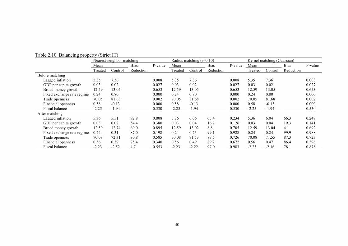
40
Table 2.10. Balancing property (Strict IT)
Nearest-neighbor matching Radius matching (r=0.10) Kernel matching (Gaussian) Mean Bias P-value Mean Bias P-value Mean Bias P-value Treated Control Reduction Treated Control Reduction Treated Control Reduction Before matching Lagged inflation 5.35 7.36 0.008 5.35 7.36 0.008 5.35 7.36 0.008 GDP per capita growth 0.03 0.02 0.027 0.03 0.02 0.027 0.03 0.02 0.027 Broad money growth 12.59 13.05 0.653 12.59 13.05 0.653 12.59 13.05 0.653 Fixed exchange rate regime 0.24 0.80 0.000 0.24 0.80 0.000 0.24 0.80 0.000 Trade openness 70.05 81.68 0.002 70.05 81.68 0.002 70.05 81.68 0.002 Financial openness 0.58 -0.13 0.000 0.58 -0.13 0.000 0.58 -0.13 0.000 Fiscal balance -2.25 -1.94 0.530 -2.25 -1.94 0.530 -2.25 -1.94 0.530 After matching Lagged inflation 5.36 5.51 92.8 0.808 5.36 6.06 65.4 0.234 5.36 6.04 66.3 0.247 GDP per capita growth 0.03 0.02 54.4 0.380 0.03 0.04 16.2 0.126 0.03 0.04 19.3 0.141 Broad money growth 12.59 12.74 69.0 0.895 12.59 13.02 8.8 0.705 12.59 13.04 4.1 0.692 Fixed exchange rate regime 0.24 0.31 87.0 0.198 0.24 0.23 99.1 0.928 0.24 0.24 99.9 0.988 Trade openness 70.08 72.31 80.8 0.585 70.08 71.53 87.5 0.726 70.08 71.55 87.3 0.723 Financial openness 0.56 0.39 75.4 0.340 0.56 0.49 89.2 0.672 0.56 0.47 86.4 0.596 Fiscal balance -2.23 -2.52 4.7 0.553 -2.23 -2.22 97.0 0.983 -2.23 -2.16 78.1 0.878
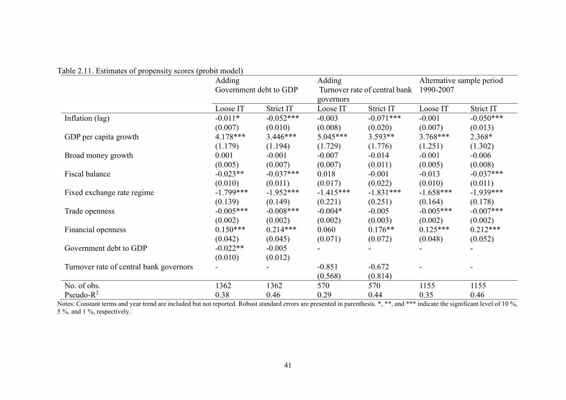
41
Table 2.11. Estimates of propensity scores (probit model)
Adding Government debt to GDP
Adding Turnover rate of central bank governors
Alternative sample period 1990-2007
Loose IT Strict IT Loose IT Strict IT Loose IT Strict IT Inflation (lag) -0.011*
(0.007) -0.052*** (0.010)
-0.003 (0.008)
-0.071*** (0.020)
-0.001 (0.007)
-0.050*** (0.013)
GDP per capita growth 4.178*** (1.179)
3.446*** (1.194)
5.045*** (1.729)
3.593** (1.776)
3.768*** (1.251)
2.368* (1.302)
Broad money growth 0.001 (0.005)
-0.001 (0.007)
-0.007 (0.007)
-0.014 (0.011)
-0.001 (0.005)
-0.006 (0.008)
Fiscal balance -0.023** (0.010)
-0.037*** (0.011)
0.018 (0.017)
-0.001 (0.022)
-0.013 (0.010)
-0.037*** (0.011)
Fixed exchange rate regime -1.799*** (0.139)
-1.952*** (0.149)
-1.415*** (0.221)
-1.831*** (0.251)
-1.658*** (0.164)
-1.939*** (0.178)
Trade openness -0.005*** (0.002)
-0.008*** (0.002)
-0.004* (0.002)
-0.005 (0.003)
-0.005*** (0.002)
-0.007*** (0.002)
Financial openness 0.150*** (0.042)
0.214*** (0.045)
0.060 (0.071)
0.176** (0.072)
0.125*** (0.048)
0.212*** (0.052)
Government debt to GDP -0.022** (0.010)
-0.005 (0.012)
- - -
-
Turnover rate of central bank governors - - -0.851 (0.568)
-0.672 (0.814)
-
-
No. of obs. 1362 1362 570 570 1155 1155 Pseudo-R2 0.38 0.46 0.29 0.44 0.35 0.46
Notes: Constant terms and year trend are included but not reported. Robust standard errors are presented in parenthesis. *, **, and *** indicate the significant level of 10 %, 5 %, and 1 %, respectively.
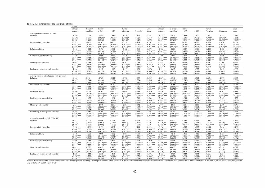
42
Table 2.12. Estimates of the treatment effects Loose IT Strict IT Nearest-
neighbor 3-nearest-neighbor
Radius Kernel Local linear
Nearest-neighbor
3-nearest-neighbor
Radius Kernel Local linear r=0.05 r=0.10 Gaussian Epanechn r=0.05 r=0.10 Gaussian Epanechn
Adding Government debt to GDP Inflation -1.150
(0.820) [0.902]
-2.026 (1.079)* [1.205]*
-1.544 (0.926)* [1.013]
-1.557 (0.897)* [1.054]
-1.518 (0.895)* [0.915]*
-1.522 (0.928) [1.023]
-1.464 (1.168) [1.972]
-1.835 (0.712)*** [0.657]***
-1.820 (0.988)* [0.729]**
-1.835 (1.035)* [0.578]***
-1.699 (0.992)* [0.550]***
-1.781 (0.984)* [0.554]***
-1.853 (1.036)* [0.598]***
-1.689 (1.361) [0.563]***
Income velocity volatility -0.183 (0.033)*** [0.035]***
-0.162 (0.037)*** [0.043]***
-0.163 (0.037)*** [0.034]***
-0.160 (0.035)*** [0.030]***
-0.159 (0.035)*** [0.033]***
-0.164 (0.037)*** [0.036]***
-0.161 (0.047)*** [0.033]***
-0.131 (0.032)*** [0.031]***
-0.069 (0.043) [0.034]**
-0.070 (0.047) [0.028]**
-0.075 (0.045)* [0.028]***
-0.076 (0.045)* [0.029]***
-0.070 (0.047) [0.028]**
-0.069 (0.057) [0.027]***
Inflation volatility -3.443 (0.477)*** [0.507]***
-3.722 (0.553)*** [0.593]***
-3.476 (0.394)*** [0.507]***
-3.471 (0.377)*** [0.500]***
-3.432 (0.377)*** [0.473]***
-3.480 (0.395)*** [0.491]***
-3.475 (0.710)*** [0.481]***
-2.923 (0.481)*** [0.532]***
-2.281 (0.636)*** [0.597]***
-2.527 (0.478)*** [0.544]***
-2.406 (0.459)*** [0.480]***
-2.400 (0.456)*** [0.460]***
-2.482 (0.478)*** [0.497]***
-2.364 (0.739)*** [0.495]***
Real output growth volatility -2.349 (0.371)*** [0.361]***
-2.770 (0.425)*** [0.556]***
-2.596 (0.255)*** [0.441]***
-2.468 (0.244)*** [0.416]***
-2.475 (0.243)*** [0.390]***
-2.590 (0.255)*** [0.459]***
-2.464 (0.493)*** [0.400]***
-2.106 (0.361)*** [0.386]***
-1.801 (0.470)*** [0.419]***
-1.875 (0.314)*** [0.335]***
-1.899 (0.302)*** [0.342]***
-1.890 (0.300)*** [0.342]***
-1.859 (0.315)*** [0.331]***
-1.831 (0.598)*** [0.340]***
Money growth volatility -1.407 (0.483)*** [0.511]***
-1.284 (0.578)** [0.613]**
-1.083 (0.556)* [0.518]**
-1.175 (0.538)** [0.497]**
-1.162 (0.538)** [0.515]**
-1.084 (0.557)* [0.510]**
-1.124 (0.627)* [0.513]**
-0.928 (0.534)* [0.537]*
-0.295 (0.680) [0.663]
-0.275 (0.673) [0.561]
-0.175 (0.652) [0.535]
-0.241 (0.648) [0.550]
-0.300 (0.673) [0.588]
-0.290 (0.834) [0.553]
Real money balance growth volatility -1.856 (0.506)*** [0.498]***
-1.639 (0.596)*** [0.591]***
-1.412 (0.552)** [0.508]***
-1.443 (0.534)*** [0.468]***
-1.419 (0.534)*** [0.510]***
-1.434 (0.553)*** [0.534]***
-1.476 (0.660)** [0.501]***
-1.421 (0.544)*** [0.555]***
-0.657 (0.703) [0.655]
-0.590 (0.669) [0.587]
-0.572 (0.649) [0.559]
-0.611 (0.645) [0.585]
-0.612 (0.669) [0.600]
-0.662 (0.815) [0.497]
Adding Turnover rate of central bank governors Inflation -0.166
(1.367) [1.467]
0.415 (1.344) [1.445]*
-0.769 (1.556) [1.289]
-0.824 (1.509) [1.251]
-0.793 (1.499) [1.226]
-0.655 (1.554) [1.312]
-0.549 (1.536) [1.313]
-2.227 (1.123)** [1.196]*
-1.948 (1.029)* [1.311]
-1.900 (1.542) [1.133]*
-2.764 (1.394)** [0.939]***
-2.631 (1.387)* [0.945]***
-1.879 (1.558) [1.072]*
-2.067 (1.389) [1.007]**
Income velocity volatility -0.231 (0.061)*** [0.061]***
-0.243 (0.055)*** [0.063]***
-0.256 (0.036)*** [0.052]***
-0.260 (0.035)*** [0.048]***
-0.257 (0.034)*** [0.050]***
-0.261 (0.036)*** [0.051]***
-0.265 (0.080)*** [0.052]***
-0.216 (0.056)*** [0.062]**
-0.258 (0.067)*** [0.072]**
-0.253 (0.051)*** [0.065]***
-0.229 (0.046)*** [0.057]***
-0.231 (0.046)*** [0.060]***
-0.259 (0.051)*** [0.063]***
-0.245 (0.071)*** [0.062]***
Inflation volatility -4.140 (0.872)*** [0.888]***
-4.029 (0.798)*** [0.957]***
-4.303 (0.581)*** [0.777]***
-4.120 (0.560)*** [0.738]***
-4.094 (0.557)*** [0.722]***
-4.284 (0.580)*** [0.790]***
-4.420 (1.092)*** [0.738]***
-4.910 (1.013)*** [1.028]***
-4.938 (0.975)*** [1.118]***
-4.746 (0.720)*** [1.025]***
-4.893 (0.657)*** [0.880]***
-4.776 (0.657)*** [0.936]***
-4.765 (0.724)*** [0.887]***
-4.813 (1.183)*** [0.972]***
Real output growth volatility -1.498 (0.458)*** [0.491]***
-1.425 (0.406)*** [0.549]***
-1.542 (0.282)*** [0.464]***
-1.601 (0.272)*** [0.459]***
-1.557 (0.270)*** [0.446]***
-1.543 (0.281)*** [0.474]***
-1.564 (0.646)** [0.457]***
-2.360 (0.639)*** [0.682]***
-2.631 (0.627)*** [0.885]***
-2.899 (0.389)*** [0.861]***
-2.634 (0.359)*** [0.725]***
-2.611 (0.359)*** [0.723]***
-2.942 (0.391)*** [0.852]***
-2.723 (0.852)*** [0.826]***
Money growth volatility -2.734 (0.869)*** [0.813]***
-2.339 (0.836)*** [0.824]***
-2.670 (0.838)*** [0.744]***
-2.560 (0.817)*** [0.722]***
-2.561 (0.813)*** [0.682]***
-2.642 (0.837)*** [0.698]***
-2.694 (0.988)*** [0.753]***
-2.866 (0.962)*** [0.999]***
-2.871 (0.940)*** [0.981]***
-2.511 (1.047)** [0.870]***
-2.511 (0.983)** [0.834]***
-2.529 (0.983)*** [0.816]***
-2.570 (1.052)** [0.818]***
-2.546 (1.083)** [0.807]***
Real money balance growth volatility -3.294 (0.930)*** [0.863]***
-2.981 (0.912)*** [0.969]***
-3.298 (0.853)*** [0.773]***
-3.198 (0.830)*** [0.758]***
-3.182 (0.826)*** [0.759]***
-3.318 (0.852)*** [0.771]***
-3.364 (1.126)*** [0.750]***
-3.595 (1.075)*** [1.079]***
-3.703 (1.052)*** [1.086]***
-3.548 (1.105)*** [1.031]***
-3.242 (1.039)*** [0.926]***
-3.328 (1.039)*** [1.003]***
-3.614 (1.110)*** [1.010]***
-3.491 (1.241)*** [1.047]***
Alternative sample period 1990-2007 Inflation -1.787
(1.275) [1.188]
-1.002 (1.379) [1.305]
-0.996 (1.097) [1.080]
-1.061 (1.067) [1.072]
-1.055 (1.061) [1.141]
-0.924 (1.100) [1.060]
-1.132 (1.794) [1.101]
-1.654 (0.779)** [0.755]**
-1.835 (0.963)* [0.818]**
-1.749 (1.234) [0.699]**
-1.991 (1.118)* [0.611]***
-1.992 (1.115)* [0.619]***
-1.732 (1.239) [0.671]***
-1.822 (1.176) [0.615]***
Income velocity volatility -0.190 (0.040)*** [0.046]***
-0.186 (0.050)*** [0.053]***
-0.195 (0.039)*** [0.037]***
-0.187 (0.037)*** [0.035]***
-0.189 (0.037)*** [0.035]***
-0.194 (0.039)*** [0.037]***
-0.194 (0.050)*** [0.032]***
-0.176 (0.040)*** [0.043]***
-0.133 (0.062)** [0.048]***
-0.095 (0.055)* [0.038]**
-0.107 (0.049)** [0.033]***
-0.104 (0.049)** [0.033]***
-0.096 (0.055)* [0.037]***
-0.108 (0.057)* [0.033]***
Inflation volatility -3.718 (0.608)*** [0.630]***
-4.008 (0.590)*** [0.719]***
-3.960 (0.446)*** [0.609]***
-3.862 (0.431)*** [0.543]***
-3.867 (0.428)*** [0.538]***
-3.988 (0.446)*** [0.550]***
-3.960 (0.782)*** [0.569]***
-3.683 (0.633)*** [0.674]***
-3.570 (0.765)*** [0.842]***
-3.458 (0.586)*** [0.689]***
-3.465 (0.530)*** [0.627]***
-3.420 (0.530)*** [0.557]***
-3.451 (0.588)*** [0.650]***
-3.494 (0.955)*** [0.604]***
Real output growth volatility -2.696 (0.457)*** [0.444]***
-2.685 (0.391)*** [0.557]***
-2.935 (0.270)*** [0.447]***
-2.862 (0.261)*** [0.394]***
-2.882 (0.258)*** [0.429]***
-2.909 (0.270)*** [0.433]***
-2.920 (0.638)*** [0.414]***
-2.717 (0.460)*** [0.523]***
-2.448 (0.554)*** [0.581]***
-2.268 (0.377)*** [0.439]***
-2.452 (0.341)*** [0.433]***
-2.404 (0.340)*** [0.408]***
-2.268 (0.378)*** [0.455]***
-2.448 (0.702)*** [0.436]***
Money growth volatility -1.635 (0.654)** [0.668]**
-1.586 (0.677)** [0.704]**
-1.457 (0.663)** [0.623]**
-1.475 (0.648)** [0.607]**
-1.473 (0.645)** [0.632]**
-1.497 (0.663)** [0.617]**
-1.457 (0.849)* [0.586]**
-0.881 (0.694) [0.729]
-0.459 (0.784) [0.798]
-0.334 (0.874) [0.807]
-0.455 (0.816) [0.753]
-0.465 (0.815) [0.682]
-0.318 (0.876) [0.771]
-0.379 (0.865) [0.732]
Real money balance growth volatility -1.520 (0.670)** [0.670]**
-1.753 (0.700)** [0.736]**
-1.618 (0.658)** [0.598]***
-1.584 (0.644)** [0.570]***
-1.566 (0.641)** [0.589]***
-1.642 (0.659)** [0.584]***
-1.596 (0.880)* [0.646]**
-1.425 (0.729)* [0.736]*
-0.767 (0.832) [0.835]
-0.543 (0.869) [0.900]
-0.674 (0.814) [0.777]
-0.661 (0.813) [0.787]
-0.534 (0.871) [0.869]
-0.637 (0.914) [0.792]
Notes: 0.06 fixed bandwidth is used for kernel and local linear regression matching. The analytical standard errors are shown in parentheses and the bootstrapped standard errors are shown in brackets (they are based on 500 replications of the data). *, ** and *** indicate the significant level of 10 %, 5% and 1%, respectively.
43
Chapter 3
Inflation targeting and exchange market pressure in
developing economies: Some international evidence
3.1 Introduction
Developing countries have frequently experienced foreign exchange market turmoil so that
the policy choice is of particular important for their macroeconomic stability. Fundamental
domestic policies, including monetary policy, may affect a country’s external sector. Since
foreign exchange markets often induce unstable external conditions, sound monetary
arrangement is required for developing economies to absorb pressures from foreign
exchange markets under a globalized world (Weymark, 1997, 1998).16 To capture such
market pressures, Girton and Roper (1977) define exchange market pressure (EMP) as the
sum of the nominal exchange rate depreciation and the percentage change of international
reserves holdings scaled by the base money (see Eichengreen et al., 1994; Bussiere &
Fratzscher, 2006; Klaassen & Jager, 2011).17 Currency depreciation only captures turmoil or
crisis initiated mainly by ‘successful’ speculative attacks that lead to deviation from the fixed
exchange rate with consequent currency depreciation. The concept of EMP incorporates
instances of ‘unsuccessful’ speculative attacks that reflect declines in international reserves
associated with monetary authority’s intervention in the foreign exchange market.
16 Weymark (1997, 1998) examine the effectiveness of exchange rate management to mitigate the EMP through changes in exchange rate or in international reserves, or both. 17 The monetary approach to the balance of payment is based on fixed exchange rate, while that to exchange rate determination is based on perfectly flexible exchange rate. However, most countries have neither a fixed nor a perfectly flexible regime. To overcome limitations of the traditional approaches, Girton and Roper (1977) develop the EMP measure, which can be used in fixed, flexible, and managed floating exchange rate regimes. In a fixed regime, the depreciation rate is zero. In a flexible regime, the change of international reserves is zero. In a managed floating regime, the exchange market pressure is absorbed by either currency depreciation, or reserve losses, or a combination of the two.
44
Inflation targeting (IT) has been adopted across advanced countries since the early
1990s. Some emerging and developing countries have also introduced an IT regime since
the late 1990s, although this regime has not been prevailed yet.18 As an IT regime is not only
a domestically focused policy framework but also related to the exchange rate regime
(Taylor, 2001; Rose, 2007), examining whether an IT adoption has any beneficial effect on
the external economy is a crucial issue for financial regulators. Although several studies
investigate the domestic effects of an IT regime, its international effects are largely
unexplored.19 Exception may include the works of Rose (2007) and Lin (2010), which
present that the IT regime helps stabilize exchange rate and accumulate international
reserves. However, past studies investigate the link of an IT regime with exchange rate and
international reserves independently and do not focus on the relationship between an IT
regime and EMP which reflects both of the two elements. Thus, this study extends the
present IT-related literature by evaluating the role of an IT regime as a monetary framework
in determining EMP in developing countries. In addition, we attempt to verify the IT effects
on the volatilities of exchange rate depreciation and international reserves changes, which
enables us to discuss how the IT adoption relates to policy stances in the foreign exchange
market.
This study applies the propensity score matching (PSM) method to mitigate self-
selection problems, following several works on the IT effects (Lin & Ye, 2007, 2009; Lin,
2010; Vega & Winkelried, 2005; de Mendonca & de Guimaraes e Souza, 2012; Samarina et
al., 2014). The main result shows clear evidence supportive of the IT role in stabilizing EMP
18 The main feature of an IT regime is an explicit quantitative inflation target and strong central bank legal commitments (e.g., Mishkin, 2000; Mishkin & Savastano, 2001). The main argument is that an official announcement of an inflation target improves a central bank’s credibility and helps to lower inflation and the volatilities of inflation and real output (see, e.g., Bernanke et al., 1999; Svensson, 1997; Mishkin, 1999). As of 2013, fifteen non-OECD countries have adopted an IT regime. 19 Recent studies on the IT effects on the domestic economic variables include Ball and Sheridan (2005), Vega and Winkelried (2005), Batini and Laxton (2007), Goncalves and Salles (2008), Lin and Ye (2009), de Mendonca and de Guimaraes e Souza (2012), Samarina et al. (2014), Thornton (2016), Kadria and Aissa (2016), and Balima et al. (2017).
45
in developing countries. In addition, our analysis of the decomposition of EMP reveals that
an IT regime helps stabilize international reserves holdings, while it does not affect exchange
rate volatility significantly. Some studies highlight that an IT regime is often related to a
floating exchange rate regime (Rose, 2007; Lin & Ye, 2009; Taylor, 2001). Hu (2006) and
Brenner and Sokoler (2010) argue that the flexibility of exchange rate motivates monetary
authority to adopt an IT regime, and its rigidity is not suitable for IT policies in the long run.
However, our results show no clear evidence that IT adoption induces exchange rate stability.
At the same time, the policy commitment to an IT regime improves the credibility of
monetary policy conduct, along with less speculative behaviors of market participants. In
this case, a central bank tends not to, or is not required to, intervene in the foreign exchange
market, so that changes in international reserves would become more stable under an IT
regime. The rest of this paper is organized as follows. Section 2 explains methodology and
the empirical results with some policy implications. Section 3 concludes.
3.2 Empirical analysis
3.2.1 Methodology
This study evaluates the IT effects on EMP over 101 developing countries from 1990 to
2014 by applying the PSM method that involves a two-step procedure. Among various
definitions of an IT adoption year, this study uses the ‘loose’ and ‘strict’ types of adoption
years, following Rose (2007), Lin (2010), and Samarina et al. (2014). A loose adoption year
represents the earliest adoption year in which inflation targets are announced without strong
commitments, and a strict adoption year represents the latest year in which credible
commitments are made to achieve inflation targets with a single inflation target via monetary
policies. This study identifies developing countries based on the IMF’s country classification,
and our treatment group includes 16 IT countries and control group contains 85 non-IT
46
countries.20 Table 3.1 shows a list of IT countries with loose and strict adoption years, and
Table 3.2 presents non-IT countries in our sample.
We apply four PSM methods. The first matching method is the nearest-neighbor
matching without replacement, which matches each treated observation to the n control
observations that have the closest propensity scores, but each control observation is used no
more than one time as a match for a treated observation. We use two nearest-neighbor
matching estimators: n = 1 and n = 3. The second method involves radius matching, where
each treated observation is matched with control observations with estimated propensity
scores that fall within a specified radius. We use two radius matching estimators: r = 0.05
and r = 0.1 . The next involves kernel matching method, which matches each treated
observation to control observations with weights inversely proportional to the distance
between the treated and control observations. We use two kernel matching methods:
Gaussian and Epanechnikov. The last matching method involves applying the regression-
adjusted local linear matching approach developed by Heckman et al. (1998).
The PSM method includes a two-step procedure. This study first applies a probit
model to estimate the propensity score, which is the conditional probability that a country
adopts an IT regime based on the country’s characteristics:
P(X) = Prob(D = 1|X) = E(D|X),
where D is a treatment or IT dummy that takes one when a country adopts an IT regime and
zero otherwise, and X is the matrix of the country’s characteristics that are expected to drive
IT regime selection, following de Mendonca and de Guimaraes e Souza (2012), Lin and Ye
20 To ensure that the treatment and control groups are comparable, Lin and Ye (2009) and Lin (2010) exclude some non-IT countries with substantially different features (e.g., real GDP per capita) from IT countries. Following their method, we exclude some non-IT countries whose real GDP per capita levels are lower than those of the smallest IT country.

47
(2007), and Samaria et al. (2014).21 The model includes the one-year lagged inflation rate,
real per capita GDP growth rate, broad money growth, and fiscal balance. To control for
external economic conditions, we also incorporate the measures of exchange rate flexibility,
trade openness, and financial openness.22 Trade openness is calculated from the ratio of the
sum of exports and imports to GDP. The data are taken from World Development Indicators
(WDI), World Economic Outlook (WEO), Reinhart and Rogoff’s (2004) de facto exchange
rate arrangement classification, and Chinn and Ito’s (2008) capital account openness index.
As a second step, we estimate the ATT by using estimated propensity scores:
ATT = E[Yi1|Di = 1] − E[Yi0|Di = 1],
where Di is the IT dummy for country i; Yi1 and Yi0 are potential outcomes of IT and non-IT
regimes (two counterfactual situations), respectively; Yi0|Di = 1 is the value of the outcome
that would have been observed if the IT country had not adopted an IT regime; and Yi1|Di =
1 is the value of the outcome that is actually observed in the same country. A crucial problem
concerns the difficulty of estimating the ATT because of the unobservable value of
E[Yi0|Di = 1]. When a country’s choice of IT regime is random, the ATT can be estimated
from differences in the sample means of the outcome variable between the groups of the IT
and non-IT countries.
21 As noted by Lin and Ye (2007), finding an appropriate statistical model that explains the probability of IT adoption is not the main goal of estimating propensity scores. Under conditional independence assumptions, the exclusion of variables that systematically affect the likelihood of IT adoption but do not affect outcome variables, such as inflation and its volatility, is not problematic in the case of probit regressions (see Persson, 2001). 22 According to Reinhart and Rogoff’s (2004) classification, the fine grid classification includes fourteen categories, and the coarse grid version aggregates these into five categories. By using the coarse grid classification, we construct the classification of the exchange rate flexibility with three categories (fixed, intermediate, and flexible).

48
However, IT regime selection is not random in the sense that such a choice is
systematically correlated with a set of observable covariates that also affect the outcome
variable, thereby creating problems in the selection of observables (e.g., Dehejia & Wahba,
2002; Heckman et al., 1998). To mitigate such a problem, we apply the PSM method, which
uses a control group of non-IT countries to mimic a randomized experiment. As suggested
by Rosenbaum and Rubin (1983), treatment and control observations can be matched based
on propensity scores p(X) to solve high-dimensional set of observed covariates. Once p(X)
is given, the ATT is estimated under two main assumptions, i.e., conditional independence
and common support assumptions, as follows:
ATT = E[Yi1|Di = 1, p(Xi)] − E[Yi0|Di = 0, p(Xi)].
3.2.2 Results
Our main interest is to determine how IT adoption affects variability of EMP in developing
countries. Since EMP is composed of exchange rate depreciation and changes in
international reserves, we attempt to evaluate IT effects by estimating the treatment effect of
an IT regime on the volatilities of each EMP component. Similar to the works of Lin (2010),
we measure the volatilities of EMP, exchange rate depreciation, and changes in international
reserves scaled by base money as the standard deviation of the twelve monthly observations
for each year. The data is obtained from International Financial Statistics (IFS). We first
estimate the propensity scores by using a probit model. Table 3.3 presents the estimation
results for the loose IT and strict IT regimes. Countries with higher inflation rates for the
previous period, sound fiscal conditions, and higher levels of trade openness are less likely
to adopt an IT regime. In addition, countries with the higher degrees of financial openness
and exchange rate flexibility are more likely to adopt an IT regime. These results generally
49
coincide with the findings of previous studies (e.g., de Mendonca & de Guimaraes e Souza,
2012; Lin & Ye, 2007; Lin, 2010).
Once the propensity scores are estimated, we estimate the ATT by applying matching
methods. We first ensure the sharing of the same support or confirm the highly and
reasonably comparability between the treatment and control groups. As in the works of Lin
and Ye (2007, 2009) and Thornton and Vasilakis (2017), we reconstruct the dataset that
satisfies the common support assumption by sorting all observations based on estimated
propensity scores and discarding control units with propensity scores that fall below the
lowest treatment unit value and exceed the highest treatment unit value.
Table 3.4 reports the ATT on the volatilities of EMP and its components for the loose
and strict IT regimes.23 The first seven columns report the results of the loose IT regime, and
the last seven show the results of the strict IT regime. Our results show that EMP volatility
is negatively significant irrespective of the choice of the IT regime, which indicates that IT
adoption helps stabilize EMP in developing countries. In addition, the results clearly show
that IT adoption reduces volatility of changes in international reserves in loose and strict IT
regimes. The average estimated ATTs on the volatilities of EMP and changes in international
reserves are about −4 ~ −2 % and −3 ~ −2 %, respectively. On the other hand, our analysis
presents no clear evidence that IT adoption would affect volatility of exchange rate changes,
although some studies suggest that an IT regime is often related to a floating exchange rate
regime (Hu, 2006; Rose, 2007; Lin & Ye, 2009; Brenner & Sokoler, 2010; Taylor, 2001).
Our analysis of the decomposition of EMP generally shows that a reduction in EMP
volatility originates from the international reserves component under an IT regime. The
policy commitment to an IT regime improves the credibility of monetary policy conduct,
23 For robustness checks, we also estimate the ATT by using an alternative sample including some non-IT countries that were excluded from our baseline analysis to ensure the comparability of treatment and control groups. The results are generally consistent with the baseline findings (see Tables 3.7 and 3.8).
50
which can mitigate speculative behaviors of market participants. Thus, once an IT regime is
adopted, central banks may not necessitate the intervention in the foreign exchange market
so that international reserves holdings become more stable.
For the better understanding, we also evaluate the IT effect for sub-samples of
developing countries by dividing our full sample of developing countries into the groups of
low- and middle-income developing countries. 24 Tables 3.5 and 3.6 report the probit
estimates and the ATTs on the volatilities of EMP and its components for each of the two
groups of low- and middle-income developing countries, respectively. Our results show clear
evidence that the IT adoption has a beneficial impact on the volatilities of EMP and changes
in international reserves in middle-income developing countries. However, our analysis fails
to present clear evidence of the IT effectiveness in low-income developing countries. These
results imply that the IT adoption would enhance the policy credibility mainly in middle-
income developing countries.
3.3 Conclusion
This study has applied the PSM method to examine whether an IT regime helps stabilize
EMP and its two components. The empirical results have indicated that an IT regime would
help stabilize EMP. In addition, our analysis has provided evidences that an IT regime
lessens volatility of changes in international reserves, while our results show no clear
evidence that an IT regime affects exchange rate variability. These findings suggest that the
policy commitment to an IT regime improves the credibility of monetary policy conduct.
Under an IT regime, central banks would not be required to intervene in the foreign exchange
market. More interestingly, our findings have also shown that an IT regime is more beneficial
for middle-income developing countries rather than for low-income developing countries.
24 The developing countries whose real GDP per capita in 2013 is below and above 6, 000 USD are classified into the low- and middle- income developing countries, respectively. For the robustness check, we also estimate our models by using the critical real GDP per capita of 8,000 USD. The results are qualitatively similar.

51
Table 3.1. Inflation targeting developing countries and starting years Country Starting Year Inflation targeting (loose) Inflation targeting (strict) Armenia 2006 2006 Brazil 1999 1999 Chile 1991 2000 Colombia 2000 2000 Ghana 2003 2007 Guatemala 2005 2006 Hungary 2001 2001 Indonesia 2005 2006 Mexico 1995 2001 Peru 2002 2002 Philippines 2002 2002 Poland 1999 1999 Romania 2005 2006 Thailand 2000 2000 Turkey 2002 2006 South Africa 2000 2000
Note: Targeting dates are taken from De Mendonca and De Guimaraes e Souza (2012), Thornton (2016), Rose (2007), and Lin and Ye (2009).
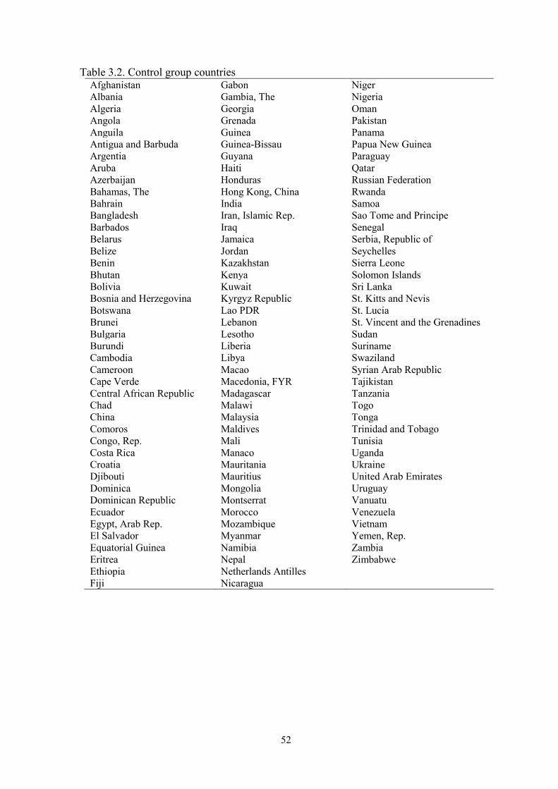
52
Table 3.2. Control group countries Afghanistan Gabon Niger Albania Gambia, The Nigeria Algeria Georgia Oman Angola Grenada Pakistan Anguila Guinea Panama Antigua and Barbuda Guinea-Bissau Papua New Guinea Argentia Guyana Paraguay Aruba Haiti Qatar Azerbaijan Honduras Russian Federation Bahamas, The Hong Kong, China Rwanda Bahrain India Samoa Bangladesh Iran, Islamic Rep. Sao Tome and Principe Barbados Iraq Senegal Belarus Jamaica Serbia, Republic of Belize Jordan Seychelles Benin Kazakhstan Sierra Leone Bhutan Kenya Solomon Islands Bolivia Kuwait Sri Lanka Bosnia and Herzegovina Kyrgyz Republic St. Kitts and Nevis Botswana Lao PDR St. Lucia Brunei Lebanon St. Vincent and the Grenadines Bulgaria Lesotho Sudan Burundi Liberia Suriname Cambodia Libya Swaziland Cameroon Macao Syrian Arab Republic Cape Verde Macedonia, FYR Tajikistan Central African Republic Madagascar Tanzania Chad Malawi Togo China Malaysia Tonga Comoros Maldives Trinidad and Tobago Congo, Rep. Mali Tunisia Costa Rica Manaco Uganda Croatia Mauritania Ukraine Djibouti Mauritius United Arab Emirates Dominica Mongolia Uruguay Dominican Republic Montserrat Vanuatu Ecuador Morocco Venezuela Egypt, Arab Rep. Mozambique Vietnam El Salvador Myanmar Yemen, Rep. Equatorial Guinea Namibia Zambia Eritrea Nepal Zimbabwe Ethiopia Netherlands Antilles Fiji Nicaragua
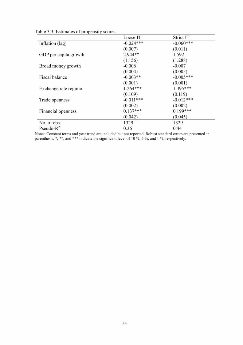
53
Table 3.3. Estimates of propensity scores Loose IT Strict IT Inflation (lag) -0.024***
(0.007) -0.060*** (0.011)
GDP per capita growth 2.944** (1.156)
1.592 (1.288)
Broad money growth -0.006 (0.004)
-0.007 (0.005)
Fiscal balance -0.003** (0.001)
-0.005*** (0.001)
Exchange rate regime 1.264*** (0.109)
1.395*** (0.119)
Trade openness -0.011*** (0.002)
-0.012*** (0.002)
Financial openness 0.137*** (0.042)
0.199*** (0.045)
No. of obs. 1329 1329 Pseudo-R2 0.36 0.44
Notes: Constant terms and year trend are included but not reported. Robust standard errors are presented in parenthesis. *, **, and *** indicate the significant level of 10 %, 5 %, and 1 %, respectively.
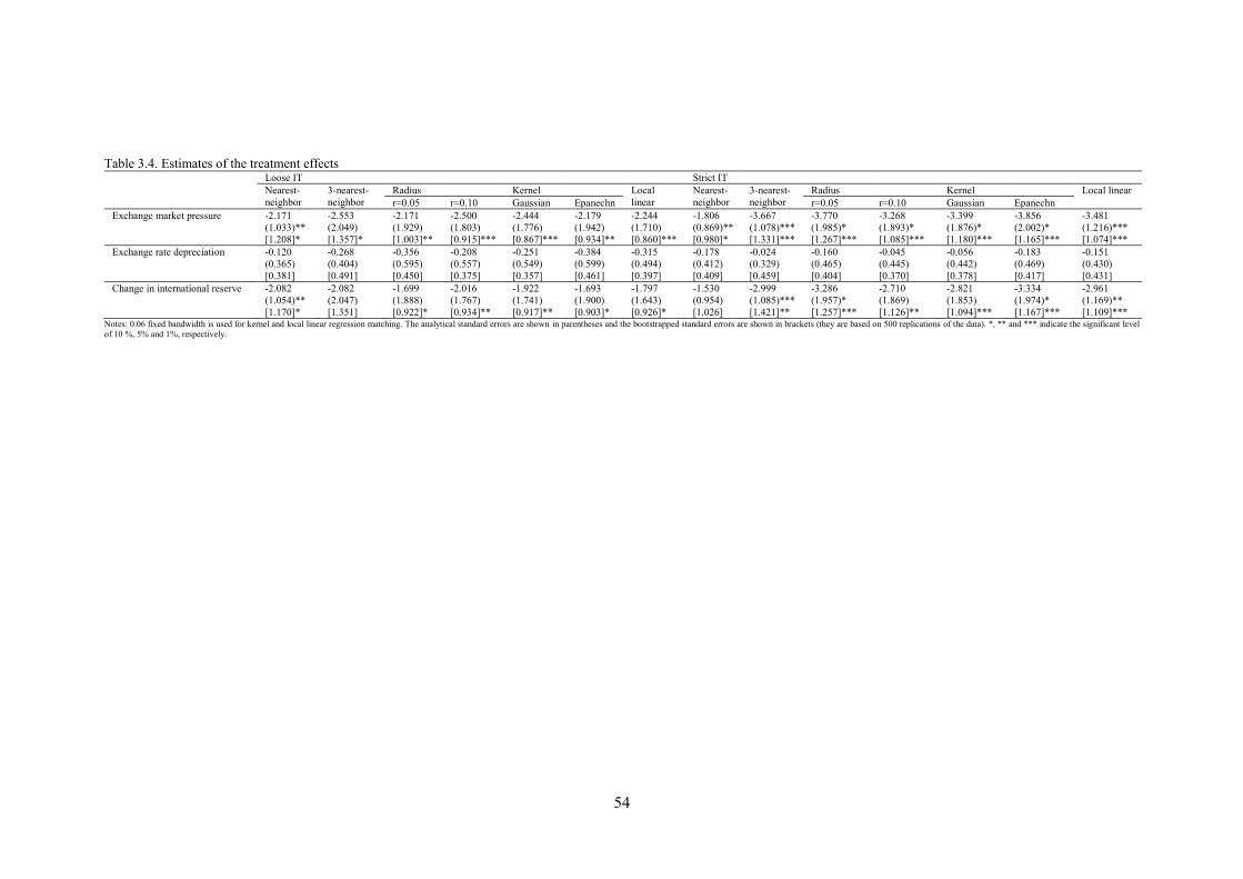
54
Table 3.4. Estimates of the treatment effects
Loose IT Strict IT Nearest-
neighbor 3-nearest-neighbor
Radius Kernel Local linear
Nearest-neighbor
3-nearest-neighbor
Radius Kernel Local linear r=0.05 r=0.10 Gaussian Epanechn r=0.05 r=0.10 Gaussian Epanechn Exchange market pressure -2.171
(1.033)** [1.208]*
-2.553 (2.049) [1.357]*
-2.171 (1.929) [1.003]**
-2.500 (1.803) [0.915]***
-2.444 (1.776) [0.867]***
-2.179 (1.942) [0.934]**
-2.244 (1.710) [0.860]***
-1.806 (0.869)** [0.980]*
-3.667 (1.078)*** [1.331]***
-3.770 (1.985)* [1.267]***
-3.268 (1.893)* [1.085]***
-3.399 (1.876)* [1.180]***
-3.856 (2.002)* [1.165]***
-3.481 (1.216)*** [1.074]***
Exchange rate depreciation -0.120 (0.365) [0.381]
-0.268 (0.404) [0.491]
-0.356 (0.595) [0.450]
-0.208 (0.557) [0.375]
-0.251 (0.549) [0.357]
-0.384 (0.599) [0.461]
-0.315 (0.494) [0.397]
-0.178 (0.412) [0.409]
-0.024 (0.329) [0.459]
-0.160 (0.465) [0.404]
-0.045 (0.445) [0.370]
-0.056 (0.442) [0.378]
-0.183 (0.469) [0.417]
-0.151 (0.430) [0.431]
Change in international reserve -2.082 (1.054)** [1.170]*
-2.082 (2.047) [1.351]
-1.699 (1.888) [0.922]*
-2.016 (1.767) [0.934]**
-1.922 (1.741) [0.917]**
-1.693 (1.900) [0.903]*
-1.797 (1.643) [0.926]*
-1.530 (0.954) [1.026]
-2.999 (1.085)*** [1.421]**
-3.286 (1.957)* [1.257]***
-2.710 (1.869) [1.126]**
-2.821 (1.853) [1.094]***
-3.334 (1.974)* [1.167]***
-2.961 (1.169)** [1.109]***
Notes: 0.06 fixed bandwidth is used for kernel and local linear regression matching. The analytical standard errors are shown in parentheses and the bootstrapped standard errors are shown in brackets (they are based on 500 replications of the data). *, ** and *** indicate the significant level of 10 %, 5% and 1%, respectively.
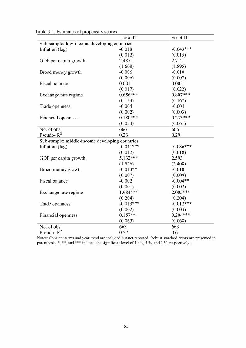
55
Table 3.5. Estimates of propensity scores Loose IT Strict IT Sub-sample: low-income developing countries Inflation (lag)
-0.018 (0.012)
-0.043*** (0.015)
GDP per capita growth 2.487 (1.608)
2.712 (1.895)
Broad money growth -0.006 (0.006)
-0.010 (0.007)
Fiscal balance 0.001 (0.017)
0.005 (0.022)
Exchange rate regime 0.656*** (0.153)
0.807*** (0.167)
Trade openness -0.004 (0.002)
-0.004 (0.003)
Financial openness
0.180*** (0.054)
0.233*** (0.061)
No. of obs. 666 666 Pseudo- R2 0.23 0.29 Sub-sample: middle-income developing countries Inflation (lag)
-0.041*** (0.012)
-0.086*** (0.018)
GDP per capita growth 5.132*** (1.526)
2.593 (2.408)
Broad money growth -0.013** (0.007)
-0.010 (0.009)
Fiscal balance -0.002 (0.001)
-0.004** (0.002)
Exchange rate regime 1.984*** (0.204)
2.005*** (0.204)
Trade openness -0.013*** (0.002)
-0.012*** (0.003)
Financial openness 0.157** (0.065)
0.204*** (0.068)
No. of obs. 663 663 Pseudo- R2 0.57 0.61
Notes: Constant terms and year trend are included but not reported. Robust standard errors are presented in parenthesis. *, **, and *** indicate the significant level of 10 %, 5 %, and 1 %, respectively.
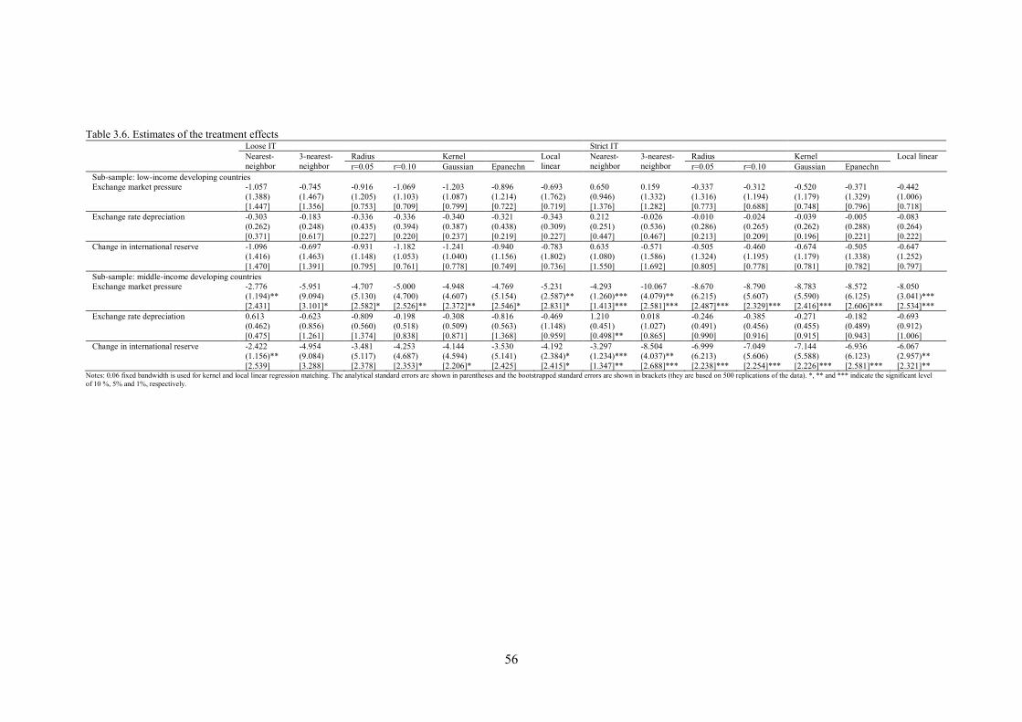
56
Table 3.6. Estimates of the treatment effects
Loose IT Strict IT Nearest-
neighbor 3-nearest-neighbor
Radius Kernel Local linear
Nearest-neighbor
3-nearest-neighbor
Radius Kernel Local linear r=0.05 r=0.10 Gaussian Epanechn r=0.05 r=0.10 Gaussian Epanechn Sub-sample: low-income developing countries Exchange market pressure
-1.057 (1.388) [1.447]
-0.745 (1.467) [1.356]
-0.916 (1.205) [0.753]
-1.069 (1.103) [0.709]
-1.203 (1.087) [0.799]
-0.896 (1.214) [0.722]
-0.693 (1.762) [0.719]
0.650 (0.946) [1.376]
0.159 (1.332) [1.282]
-0.337 (1.316) [0.773]
-0.312 (1.194) [0.688]
-0.520 (1.179) [0.748]
-0.371 (1.329) [0.796]
-0.442 (1.006) [0.718]
Exchange rate depreciation -0.303 (0.262) [0.371]
-0.183 (0.248) [0.617]
-0.336 (0.435) [0.227]
-0.336 (0.394) [0.220]
-0.340 (0.387) [0.237]
-0.321 (0.438) [0.219]
-0.343 (0.309) [0.227]
0.212 (0.251) [0.447]
-0.026 (0.536) [0.467]
-0.010 (0.286) [0.213]
-0.024 (0.265) [0.209]
-0.039 (0.262) [0.196]
-0.005 (0.288) [0.221]
-0.083 (0.264) [0.222]
Change in international reserve -1.096 (1.416) [1.470]
-0.697 (1.463) [1.391]
-0.931 (1.148) [0.795]
-1.182 (1.053) [0.761]
-1.241 (1.040) [0.778]
-0.940 (1.156) [0.749]
-0.783 (1.802) [0.736]
0.635 (1.080) [1.550]
-0.571 (1.586) [1.692]
-0.505 (1.324) [0.805]
-0.460 (1.195) [0.778]
-0.674 (1.179) [0.781]
-0.505 (1.338) [0.782]
-0.647 (1.252) [0.797]
Sub-sample: middle-income developing countries Exchange market pressure -2.776
(1.194)** [2.431]
-5.951 (9.094) [3.101]*
-4.707 (5.130) [2.582]*
-5.000 (4.700) [2.526]**
-4.948 (4.607) [2.372]**
-4.769 (5.154) [2.546]*
-5.231 (2.587)** [2.831]*
-4.293 (1.260)*** [1.413]***
-10.067 (4.079)** [2.581]***
-8.670 (6.215) [2.487]***
-8.790 (5.607) [2.329]***
-8.783 (5.590) [2.416]***
-8.572 (6.125) [2.606]***
-8.050 (3.041)*** [2.534]***
Exchange rate depreciation 0.613 (0.462) [0.475]
-0.623 (0.856) [1.261]
-0.809 (0.560) [1.374]
-0.198 (0.518) [0.838]
-0.308 (0.509) [0.871]
-0.816 (0.563) [1.368]
-0.469 (1.148) [0.959]
1.210 (0.451) [0.498]**
0.018 (1.027) [0.865]
-0.246 (0.491) [0.990]
-0.385 (0.456) [0.916]
-0.271 (0.455) [0.915]
-0.182 (0.489) [0.943]
-0.693 (0.912) [1.006]
Change in international reserve -2.422 (1.156)** [2.539]
-4.954 (9.084) [3.288]
-3.481 (5.117) [2.378]
-4.253 (4.687) [2.353]*
-4.144 (4.594) [2.206]*
-3.530 (5.141) [2.425]
-4.192 (2.384)* [2.415]*
-3.297 (1.234)*** [1.347]**
-8.504 (4.037)** [2.688]***
-6.999 (6.213) [2.238]***
-7.049 (5.606) [2.254]***
-7.144 (5.588) [2.226]***
-6.936 (6.123) [2.581]***
-6.067 (2.957)** [2.321]**
Notes: 0.06 fixed bandwidth is used for kernel and local linear regression matching. The analytical standard errors are shown in parentheses and the bootstrapped standard errors are shown in brackets (they are based on 500 replications of the data). *, ** and *** indicate the significant level of 10 %, 5% and 1%, respectively.
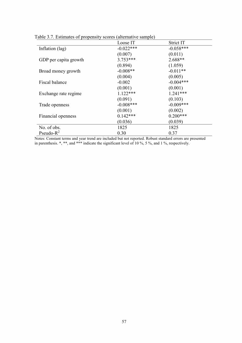
57
Table 3.7. Estimates of propensity scores (alternative sample)
Loose IT Strict IT Inflation (lag) -0.022***
(0.007) -0.058*** (0.011)
GDP per capita growth 3.753*** (0.894)
2.688** (1.059)
Broad money growth -0.008** (0.004)
-0.011** (0.005)
Fiscal balance -0.002 (0.001)
-0.004*** (0.001)
Exchange rate regime 1.122*** (0.091)
1.241*** (0.103)
Trade openness -0.008*** (0.001)
-0.009*** (0.002)
Financial openness 0.142*** (0.036)
0.200*** (0.039)
No. of obs. 1825 1825 Pseudo-R2 0.30 0.37
Notes: Constant terms and year trend are included but not reported. Robust standard errors are presented in parenthesis. *, **, and *** indicate the significant level of 10 %, 5 %, and 1 %, respectively.
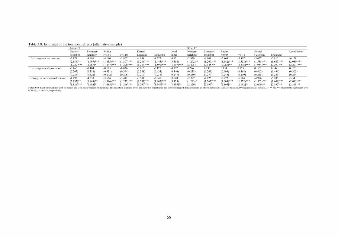
58
Table 3.8. Estimates of the treatment effects (alternative sample)
Loose IT Strict IT Nearest-
neighbor 3-nearest-neighbor
Radius Kernel Local linear
Nearest-neighbor
3-nearest-neighbor
Radius Kernel Local linear r=0.05 r=0.10 Gaussian Epanechn r=0.05 r=0.10 Gaussian Epanechn Exchange market pressure -5.171
(2.184)** [1.729]***
-4.986 (1.907)*** [2.767]*
-4.190 (1.435)*** [1.447]***
-3.967 (1.307)*** [1.290]***
-4.058 (1.286)*** [1.284]***
-4.372 (1.445)*** [1.591]***
-4.121 (3.514) [1.397]***
-2.879 (1.292)** [2.475]
-4.809 (1.269)*** [2.145]**
-5.869 (1.642)*** [2.287]**
-5.807 (1.558)*** [2.235]***
-5.627 (1.538)*** [1.954]***
-5.810 (1.647)*** [2.290]**
-6.179 (2.080)*** [2.293]***
Exchange rate depreciation -0.166 (0.267) [0.284]
-0.104 (0.318) [0.322]
-0.125 (0.431) [0.242]
-0.036 (0.394) [0.206]
-0.013 (0.388) [0.219]
-0.120 (0.434) [0.238]
-0.152 (0.346) [0.247]
0.296 (0.238) [0.239]
0.190 (0.249) [0.279]
0.154 (0.493) [0.245]
0.175 (0.468) [0.239]
0.187 (0.462) [0.235]
0.144 (0.494) [0.243]
0.102 (0.303) [0.244]
Change in international reserve -4.492 (2.133)** [1.821]***
-4.330 (1.863)** [2.484]*
-3.664 (1.396)*** [1.415]***
-3.411 (1.272)*** [1.266]***
-3.504 (1.251)*** [1.260]***
-3.841 (1.405)*** [1.549]***
-3.548 (3.435) [1.395]**
-2.397 (1.293)* [2.229]
-4.126 (1.263)*** [2.199]*
-5.272 (1.603)*** [2.195]**
-5.164 (1.522)*** [2.192]**
-4.976 (1.503)*** [2.000]**
-5.205 (1.608)*** [2.192]**
-5.541 (2.085)*** [2.318]**
Notes: 0.06 fixed bandwidth is used for kernel and local linear regression matching. The analytical standard errors are shown in parentheses and the bootstrapped standard errors are shown in brackets (they are based on 500 replications of the data). *, ** and *** indicate the significant level of 10 %, 5% and 1%, respectively.
59
Chapter 4
Inflation targeting and central bank credibility: Any
difference between advanced and developing economies?
4.1 Introduction
Since monetary policy is a useful tool to quickly, but temporarily, achieve macroeconomic
objectives, central banks influenced by political or governmental authorities tend to
emphasize short-term economic expansions, leading to the inflationary policy bias
(Cukierman, 1994; Walsh, 2005). One possible solution to mitigate such a policy bias is to
allow central banks to be sufficiently independent from political influences in stabilizing
inflation, thereby enhancing their credibility in financial markets. Indeed, many countries,
particularly advanced countries, have granted autonomy to their monetary authorities in the
past few decades. The monetary autonomy issue is more substantial in developing countries
than it is in advanced countries. Fry (1998) suggests that macroeconomic policy including
monetary policy in developing countries is often dominated by government fiscal positions.
According to his fiscal dominance hypothesis of central bank independence, the size of the
government`s deficit and the methods by which it is financed determine the central banks’
independence in developing countries. In line with these arguments, the notion of central
bank independence (CBI) has emerged as an effective means of insulating monetary policy
from political interference to achieve long-term economic stability without the monetization
of public debt and the loss of inflation-fighting credibility (Bernhard, 2002; Garriga, 2016;
Eijffinger & De Haan, 1996).25
25CBI generally refers to the freedom of monetary policymakers from direct political or governmental influence in the conduct of policy. Bernhard (2002) and Garriga (2016) argue that CBI is the central bank’s ability to control the instrument of monetary policy or, in contrast, is the set of restrictions to the influence of the government on the central bank’s arrangement of monetary policy. Eijffinger and De Haan(1996) highlight
60
The conventional theory on central bank independence relates to the inflationary bias
inherent in monetary policy due to the time inconsistency problem (Kydland & Prescott,
1977; Barro & Gordon, 1983). The ‘rules versus discretion’ literature initiated by Barro and
Gordon (1983) and Rogoff (1985) suggests that the credible delegation of monetary control
to an independent central bank can mitigate the time-inconsistency problem and the
inflationary bias.26 From empirical perspectives, most political scientists and economists
generally agree with the theoretical argument that central bank independence lowers
inflation. There have been many empirical studies performed on the role of central bank
independence relating to various aspects, such as monetary policy, financial liberalization,
political institutions, democratization, or responses to crises (Adam et al., 2011; Klomp &
de Haan, 2009; Reenock et al., 2013; Rosas, 2006). Among them, some works, including
Klomp and de Haan (2009) and Lohmann (2006), argue that central bank independence
contributes to achieving price stability as well as financial stability.
In the past, central banks tended to maintain confidentiality with less transparency.
Some were engaged in commercial banking operations and did not release much information
about public finances. However, the recent trend of central bank independence has demanded
accountability, legitimacy considerations and guidance, which call for central bank
transparency (CBT) (Crowe & Meade, 2008; Dincer & Eichengreen, 2014).27 Transparency
three types of independence of the central banks, such as personnel, financial, and policy independence. Personnel independence is the limitation to the influence of the government on the membership or tenure of the central bank board. Financial independence reflects restrictions to the capability of the government to use the central bank’s loans to finance government budget deficits. Policy independence implies the central bank’s ability to formulate and implement the monetary policy, such as setting the goals and/or choosing the monetary policy instrument to achieve its primary objective. 26For the economics literature, see, e.g., Barro and Gordon (1983a, 1983b), Rogoff (1985), Lohmann (1992), Cukierman (1992), and Eijffinger and De Haan (1996). For the political science literature, see, e.g., Hirsch and Goldthorpe (1978), Beck (1984), Woolley (1984), Lindberg and Maier (1985), Mayer (1990), and Goodman (1992). 27Dincer and Eichengreen (2014) highlight that the rise of central bank transparency can be seen as (1) improving the government’s response to the public; (2) a crucial element of accountability or a mechanism allowing the public to assess the consistency of the central bank’s actions with a mandate; (3) a way of making market participants more smoothly responsive to monetary policy decisions; and (4) a method of enhancing the credibility of the central bank’s commitment.
61
is an inverse concept of confidentiality. Transparency can be regarded as a necessary
mechanism, which enables the public to assess the consistency of a central bank’s actions
with its mandate and allows the private sector and financial operators to improve their
expectations and business decisions (Blinder, 1998; Van der Cruijsen & Demertzis, 2007;
Crowe & Meade, 2008). In addition, central bank transparency improves policy credibility
as well as policy flexibility. A credible commitment makes a central bank flexible to deviate
from a policy target when exceptional conditions occur since the public clearly understands
that the deviation is temporary without an inconsistency with long-term targets.
Since the early 1990s, inflation targeting (IT) has been widely adopted as an
alternative monetary policy framework in advanced countries. Since the late 1990s, some
emerging and developing countries have also introduced an IT regime, although this regime
is not yet prevalent in all developing and emerging countries.28 The main feature of an IT
regime is an explicit quantitative inflation target and strong central bank legal commitment
to the transparency, accountability, and credibility of price stability when implementing
monetary policies (Mishkin, 2000; Mishkin & Savastano, 2001). The argument underlying
this feature is that an official announcement of an inflation target improves a central bank’s
credibility and helps to lower inflation and the volatilities of inflation and real output
(Bernanke et al., 1999; Svensson, 1997; Mishkin, 1999).
The conventional view is that the adoption of an IT regime as a reform in the
monetary policy context increases the transparency of monetary policy conduct (Bernanke
et al., 1999; Faust & Henderson, 2004; Mishkin & Schmidt-Hebbel, 2007; Mishkin &
Schmidt-Hebbel, 2002; Svensson, 1999). Crowe (2010) suggests that IT adoption
contributes to the convergence in forecast errors, implying that it improves transparency. In
addition, some studies, including Mishkin (1999) and Freedman and Otker-Robe (2010),
28Indeed, as of 2012, there were 12 advanced economies and 17 emerging and developing countries, according to the IMF classification (De Mendonca & De Guimaraes e Souza, 2012).

62
discuss the relationship between the introduction of IT and the independence of central banks.
Mishkin (1999) argues that an IT regime can eliminate the political pressure on central banks
to implement expansionary policies since it enables central banks to focus on price stability
in the long run. Freedman and Otker-Robe (2010) highlight that IT countries have passed
legislation providing the central bank with the authority to control monetary policy. In spite
of growing debates on institutional reforms of central banks, few empirical studies have
examined how IT adoption affects central banks’ transparency and independence as the
institutional reforms, which are closely related to their credibility. Although several studies
show the favorable macroeconomic effects of an IT regime, its direct impact on central bank
independence and transparency in advanced and developing countries is still unexplored.29
In addition, the central banks’ institutional reform has become more important for
developing countries that often face economic and financial instability as well as political
pressures. Thus, this study attempts to extend the present IT-related literature by addressing
such issues in both advanced and developing countries and to discuss the differences between
them.
This study investigates how IT adoption relates to the transparency and independence
of central banks by applying the entropy balancing method to mitigate self-selection
problems, following several works on the treatment effects (Neuenkirch & Neumeier, 2016;
Huang & Yeh, 2014). Policy debates have been conducted to determine the countries that
have actually adopted the IT regime in an effective manner (Caballero & Krishnamurthy,
29Recent studies on the IT effects on the domestic economic variables include Ball and Sheridan (2005),Vega and Winkelried (2005), Batini and Laxton (2007), Goncalves and Salles (2008), Lin and Ye (2009), de Mendonca and de Guimaraes e Souza (2012), Samarina et al. (2014),and Thornton (2016). Several works have studied the effects of IT regimes on some macroeconomic conditions other than inflation, inflation volatility, and output volatility via the PSM method. For example, Lin (2010) shows that the IT regime reduces levels of real and nominal exchange rate volatility, while increasing international reserves in developing countries, although it intensifies the exchange rate instability and reduces international reserves in advanced economies. Lucotte (2012) indicates that IT regimes have a positive significant effect on tax revenue collection in developing countries. Kadria and Aissa (2016) conclude that an IT regime can help reduce budget deficits in developing economies. Balima et al. (2017) show that IT adoption reduces levels of sovereign debt risk.

63
2005; Mishkin, 2004; Sims, 2005; Svensson, 1997). Among various definitions of an
adoption year, this study uses the ‘loose’ and ‘strict’ types of adoption years, following Rose
(2007), Lin (2010), and Samarina et al. (2014). A loose adoption year represents the earliest
adoption year in which inflation targets are announced without strong commitments, and a
strict adoption year represents the latest year in which credible commitments are made to
achieve inflation targets with a single inflation target via monetary policies. Moreover, this
study attempts to examine heterogeneous features of the performance of an IT regime, as in
the work of Carare and Stone (2006), Mishkin (2004), and Fraga et al. (2003). To check the
validity of the results derived from the entropy balancing method, this study further applies
the standard panel approaches, including the dynamic panel estimation method developed
by Arellano and Bover (1995) and Blundell and Bond (1998), as alternative methods, as in
the works of Neuenkirch and Neumeier (2016).
The empirical analysis shows several important findings. First, the entropy balancing
approach presents clear evidence supportive of the role of IT in improving central bank
transparency in both advanced and developing countries. Second, more importantly, the
results suggest a clear difference between advanced and developing countries in the IT
effects on central bank independence. Advanced countries that have adopted an IT regime
experience higher central bank independence, while developing countries with an IT
adoption experience lower central bank independence. The standard panel approaches as
alternative methods confirm the empirical validity of the results of the entropy balancing
analysis. The negative effect of an IT regime on central bank independence in developing
countries may reflect the argument in the political economy context that central banks are
granted stringent monetary authority in pursuit of price stability at the expense of losing
independence from political authorities that often tend to keep central banks under their
authority.
64
Third, our analysis also presents heterogeneous effects on transparency and the
independence of central banks. Concerning the IT effects on transparency, a more flexible
exchange rate causes an IT regime to be less effective at improving transparency in advanced
countries, while it causes an IT regime to be more effective at improving transparency in
developing countries. Regarding the role of fiscal discipline in the effectiveness of an IT
regime, developing countries with a high fiscal discipline have less motivation to improve
transparency. On the other hand, the heterogeneous effects on independence reveal that the
higher flexibility of the exchange rate causes an IT regime to be less effective at improving
independence in advanced countries. In addition, the negative effect of an IT regime on
independence decreases over time in developing countries.
The rest of this paper is organized as follows. Section 2 presents a literature review
on the adoption of IT, central bank independence and transparency. In section 3, we estimate
the average treatment effects on the treated (ATT) by applying entropy balancing methods.
Then, we present our empirical results of the IT effects on central bank transparency and
independence and discuss their intuitions by identifying their differences between advanced
and developing countries. Section 4 presents our conclusions.
4.2 Literature review
4.2.1 Measures of central bank independence and transparency
Since the 1990s, many central banks in advanced countries have started adopting an IT
regime and the credibility of a central bank has become more important for monetary
authorities because a lower level of central bank credibility leads to less effectiveness of
monetary policy. Central bank independence (CBI) and central bank transparency (CBT)
might play a crucial role in improving the credibility of central banks since they may reduce
time inconsistency problems of monetary policy and enable market participants to assess the
consistency of a central bank’s actions with its mandate. With the increasing importance of

65
credibility in the conduct of monetary policy, we need appropriate measurements of CBI and
CBT to capture the credibility of a central bank’s monetary policy.
Cukierman (1994) highlights that there are four main types of CBI indices, such as
legal indices derived from the charters of central banks, questionnaire-based indices, the
actual turnover of central bank governors, and the political vulnerability of central banks.
Some studies use measures of de facto CBI, which are based on questionnaires (Blinder,
2000; Cukierman et al., 1992; Fry et al., 1996) or in terms of the turnover rate of central bank
governors (Cukierman & Webb, 1995; Cukierman et al., 1992; De Haan & Siermann, 1996).
The measures based on questionnaires may be less reliable partly because of their narrow
coverage, problematic cross-sectional comparability, and little within-country variation
(Garriga, 2016). Cukierman et al. (1992) suggests that the central bank governors’ turnover
rate is an appropriate measure in predicting the impact of CBI in developing countries.
Many empirical studies also apply de jure measures of CBI based on central banks
statutes instead of applying de facto measures (Alesina et al., 1989; Cukierman, 1992;
Cukierman, et al., 1992; Grilli et al., 1991). Alesina et al. (1989) and Grilli et al. (1991) build
de jure measures of CBI based on various factors, such as political, financial, and economic
independence.30 Cukierman et al. (1992) construct the CBI index (the CWN index) based on
30Alesina et al. (1989) construct the CBI index partly based on studies by Masciandaro and Tabellini (1988) that consider two dimensions of independence, such as political independence (the central bank’s ability to formulate and implement the monetary policy, such as setting the goals and/or choosing the monetary policy instrument) and financial independence (the degree of restrictions to the government’s ability to use central bank’s loans to finance government budget deficits).Alesina et al. (1989) emphasizes the criterion related to political aspects and suggest that the degree of CBI is affected by four main criteria: (i) institutional and formal relationships between central banks and the executives (for instance, the identification of the responsibility for (and frequency of) the appointment of a central bank’s governor, the presence of government officials on the board of directors of central banks, and the requirements of the government's approval of specific policies); (ii) informal relationships and contacts between a central bank and executive members; (iii) budgetary and financial relationships between a central bank and the executive; and (iv) macroeconomic relationships, such as the existence of rules forcing a central bank to accommodate fiscal policy.
Grilli et al. (1991) distinguish two types of CBI: political independence (the ability of a central bank to choose the objectives of monetary policy) and economic independence (the ability of a central bank to choose its instruments). They measure political independence based on three aspects of a monetary regime: (i) the procedure for appointing the members of the central bank government bodies; (ii) the relationship between these bodies and the government; and (iii) the formal responsibilities of the central bank. In addition, they measure economic independence based on (i) the influence of the government in determining how much to
66
the legal independence reflecting the independence of the chief executive officer (CEO) of
the central bank, the central banks’ independence in policy formation, its objective or
mandate, and the stringency of limits on its lending to the public sector. Recently, Dincer
and Eichengreen (2014) elaborate de jure measures of CBI by incorporating some legal
aspects, such as limits on the reappointment of the CEO and board members, restrictions on
government representation on the board, and the intervention of the government in exchange
rate policy formulation, into the criteria of the CWN index. In addition, Garriga (2016)
constructs the comprehensive dataset on the de jure CBI measures that identify statutory
reforms affecting the CBI, their direction, and the attributes necessary to build the CWN
index. Garriga (2016) highlights that de jure measures are suitable to explore the
determinants of the independence of monetary institutions, although the indices of legal CBI
have been criticized. 31 Bodea and Hicks (2014) also attempt to code CBI information
annually and directly identify reform years in their coding of the reforms of the past twenty-
five years. They code the texts of approximately 80 countries for the year 1973 to 2008 to
update the CWN index of CBI. CWN’s original data covers 72 countries for four decades
(1950–59, 1960–72, 1973–79, and 1980–89). Recently, Bodea and Hicks (2015) updated
their CBI data for 144 countries, covering the period from 1972 to 2015.
Regarding the measurement of central bank transparency (CBT), Fry et al. (2000) is
the first study to construct comprehensive measures of CBT. The strength of the measures
of Fry et al.(2000) is its wide country coverage based on a survey of 94 central banks, and
its limitation is the relatively restrictive definition of transparency. Fry et al. (2000) measure
borrow from the central bank; and (ii) the nature of the monetary instruments under the control of the central bank. Debelle and Fischer (1994) define political and economic independence as a goal and instrument independence, respectively. Arnone et al. (2009) also construct the CBI indicator based on the methodology proposed by Grilli et al. (1991). 31 De jure measures are often criticized since laws do not consider all possible conditions that might affect the relationships between a central bank and the government. Moreover, the facts described in the laws often deviate from the actual practices, especially in developing countries, and even independent central banks can be influenced by the government’s appointments and threats to the bank (Lohmann, 1998).

67
transparency based on an equally weighted average of three indicators: (i) whether a central
bank provides prompt public-explanations of its policy decisions; (ii) the frequency and form
of forward-looking analysis provided to the public; and (iii) the frequency of bulletins,
speeches, and research papers.32 Eijffinger and Geraats (2006) distinguish more aspects of
transparency and consider more than one point in time. Their indices distinguish political
transparency (openness about policy objectives), economic transparency (openness about
data, models, and forecasts), procedural transparency (openness about the way decisions are
made, achieved mainly through the release of minutes and votes), policy transparency
(openness about the policy implications, achieved through prompt announcement and
explanation of decisions), and operational transparency (openness about the implementation
of those decisions—in other words, about control errors and macroeconomic disturbances
affecting their magnitude). The advantage of this approach is its comprehensiveness,
including multi-dimensional definitions of transparency, but its limitation is that the
transparency index is constructed for only nine central banks.
In general, most studies measure CBT using either a very limited number of central
banks or a single point in time. Following the five elements of Eijffinger and Gerrats (2006),
Crowe and Meade (2008) construct the measures of CBT covering 37 central banks over 2
periods. Dincer and Eichengreen (2007) replicate and extend the indices of Eijffinger and
Geraats (2006), and Dincer and Eichengreen (2014) update their CBT index covering over
100 central banks during 13 periods (1998 to 2010). This study uses the indices of CBI and
CBT constructed by Dincer and Eichengreen (2014) in our baseline analysis. For the
robustness check, we also consider the CBI index of Garriga (2016) and Bodea and Hicks
(2015) as alternative measures of CBI.
32 Chortareas et al. (2002, 2003) adopt a slightly different approach, focusing on two aspects of CBT: (i) the publication of forecasts and (ii) the release of information on the monetary policy decisions; these two aspects correspond broadly to the categories of economic transparency and policy transparency, respectively.
68
4.2.2 Consequences and determinants of central bank independence and
transparency
Achieving macroeconomic and financial stability requires monetary policy credibility,
which is closely related to CBI and CBT. 33 Concerning the consequences of CBI, an
independent central bank can control inflation through the reduction of the risk of time
inconsistency in monetary policy (Kydland & Prescott, 1977; Barro & Gordon, 1983; Haga,
2015). Many studies show a negative effect of CBI on inflation, mainly focusing on
advanced countries (Grilli et al., 1991; Cukierman, 1992; Cukierman et al., 1992; Alesina &
Summers, 1993; Eijffinger et al., 1998; Crowe & Meade, 2008; Dincer & Eichengreen,
2014).34 However, some studies have doubted the negative relationship between CBI and
inflation (Campillo & Miron, 1997; Forder, 1998; King & Ma, 2001; Daunfeldt & de Luna,
2008; Jacome & Vasquez, 2008). Ismihan and Ozkan (2004) provide a theoretical
explanation for the less significant relationship between CBI and inflation, arguing that
although CBI contributes to lower inflation in the short term, the effects on growth make
CBI less likely to achieve lower inflation in the long-term. Thus, the relationship between
CBI and inflation is still controversial particularly in developing countries. Some studies
suggest that CBI is significantly and negatively related to inflation in developing countries
(Cukierman, 1992; Cukierman et al., 1992; De Haan & Kooi, 2000; Brumm, 2006; Garriga,
2016), while others fail to present clear linkages between CBI and inflation in developing
33Both transparency and independence tend to enhance credibility (Eijffinger & Hoeberichts, 2002). Eijffinger et al. (2006) indicate that transparency increases central bank credibility, flexibility and reputation. 34Dreher et al. (2008) suggest the possibility of a reverse relationship between inflation and CBI, often based on turnover rates, since central bankers who have failed to control inflation have often been replaced. In addition, some studies examine how CBI not only relates to inflation but also to other macroeconomic conditions, such as inflation volatility and output, and the credibility of monetary policy (Bodea & Hicks, 2015; Cukierman, 1992; Cukierman et al., 2002; Cukierman et al., 1992; Persson & Tabellini, 1990; Rogoff, 1985; Dincer & Eichengreen, 2014; Garriga, 2016). Moreover, some empirical studies focus on the association between CBI and financial market performance (Klomp & de Haan, 2009; Kuttner & Posen, 2010; Moser & Dreher, 2010; Forch & Sunde, 2012).
69
countries (Cukierman, 1992; Cukierman et al., 1992; Campillo & Miron, 1997; Ismihan &
Ozkan, 2004; Arnone et al., 2009; Sturm & de Haan, 2001).
Regarding the consequences of CBT, many studies explore its effects on
macroeconomic variables, including inflation and variabilities of inflation and output, using
various forms of transparency. 35 By employing the CBT index of Fry et al. (2000),
Chortareas et al. (2002) find that information disclosure reduces inflation, and Cecchetti and
Krause (2002) show that a better macroeconomic performance consisting of inflation and
output variabilities is associated with the transparency of central banks rather than with their
independence. In addition, by using the index of CBT constructed by Demertzis and Hallett
(2007) indicate that CBT helps reduce inflation variability but its impacts on the level of
inflation and output and the variability of output in nine OECD countries are less clear.
Moreover, Dincer and Eichengreen (2007, 2014) construct the index of CBT and find that
transparency lowers inflation and the variabilities of inflation and output.
Although many studies exist on the consequences of CBI and CBT, a relatively small
number of empirical studies explore their determinants. D’Amato et al. (2009) evaluate the
determinants of CBI and present that OECD countries experiencing higher inflation with
lower political instability have more incentive to increase CBI, while non-OECD countries
with more trade openness, higher GDP per capita, higher inflation, and less developed fiscal
systems tend to have greater CBI. Dincer and Eichengreen (2014) also evaluate the
determinants of CBI and suggest that independence is likely to increase in countries with
trade openness under IMF programs, while it tends to decrease in countries with a British
35Studies on the effect of transparency on financial markets also provide favorable results. Fratzscher (2006) suggests that transparency lowers the exchange rate volatility and uncertainty. De Goeij and Marquering (2006) and Ranaldo and Rossi (2010) find that the bond market reacts significantly to central bank communication. Neuenkirch (2012) provides the evidence that transparency lowers the bias in money market expectations and dampens their variation. Reeves and Sawicki (2007) suggest that the publication of the inflation report lowers stock market volatility. Papadamou et al. (2014) provide the empirical evidence that transparency helps stabilize stock market volatility, implying that it is beneficial for maintaining financial stability.
70
legal practice. Dincer and Eichengreen (2007, 2014) generally highlight the determinants of
CBT and confirm that transparency is greater in countries with high-income levels, flexible
exchange rate regimes, developed financial markets, and stable political systems.
4.2.3 Inflation targeting
During the past decades, the IT regime has been widely adopted by several central banks as
a policy measure. On the theoretical front, clear predictions have not been made regarding
the effectiveness of IT adoption. Several studies, including Bernanke and Woodford (2005),
Caballero and Krishnamurthy (2005), Mishkin (2000, 2004), and Sims (2005), suggest that
the current lack of institutional development and inconsistencies among macroeconomic
conditions in developing countries could undermine the success of IT and result in worse
outcomes. However, a number of other studies, such as Svensson (1997), Mishkin (1999),
and Bernanke et al. (1999), argue that as the credibility of central banks is initially low in
emerging economies, the adoption of IT renders monetary policies more credible, thereby
contributing to better macroeconomic outcomes in these economies.
Some empirical studies investigate the driving factors for central banks to adopt the
IT regime as a monetary policy conduct. Hu (2006) suggests that a country’s decision to
adopt an IT regime may be influenced by several economic and institutional factors, such as
fiscal position, financial depth, exchange rate flexibility, and the monetary autonomy of the
central bank. Goncalves and Carvalho (2008, 2009) indicate that countries with lower debts,
higher inflation, and flexible exchange rates are more likely to adopt an IT regime. Ismailov
et al. (2016) find that the desires to keep or enhance anti-inflation credibility and a more
flexible exchange rate without a nominal exchange rate anchor are the main driving forces
to adopt an IT regime in high-income countries, while a high level of debts may hinder the
countries’ desirability of IT adoption in low-income countries. On the other hand, there have
been many empirical studies on how an IT regime affects macroeconomic variables. Among
71
them, Vega and Winkelried (2005), Lin and Ye (2007, 2009), De Mendonca and de
Guimaraes e Souza (2012), and Samarina et al. (2014) indicate that IT adoption lowers
inflation, inflation volatility, and output volatility. 36 The possible reason of the IT
effectiveness is that central banks may improve the credibility of their monetary policy by
the adoption of the IT regime.
In contract to many works on the macroeconomic effects of an IT regime, a relatively
small number of empirical studies have been conducted on its impacts on the central bank’s
institutional structure reforms, particularly on CBI and CBT. Mishkin (1999) and Batini and
Laxton (2007) discuss that an IT adoption would promote greater de facto or de jure
independence of the central bank since its adoption focuses on price stability and is
associated with less political pressure to implement expansionary policies. Mishkin and
Schmidt-Hebbel (2002) suggest that an IT regime is associated with a greater increase in
transparency and accountability. To the best of our knowledge, few comprehensive empirical
studies have been conducted regarding the impacts of an IT regime on transparency and the
independence of central banks (CBT and CBI). In addition, the central banks’ institutional
reform has become more important for developing countries that often face economic and
financial instability as well as political pressures. Thus, this study attempts to extend the
present IT-related literature by addressing such issues in both advanced and developing
countries and to discuss the difference between them.
36Several works have studied the effects of IT regimes on some macroeconomic conditions other than inflation, inflation volatility, and output volatility. For example, Lin (2010) shows that the IT regime reduces levels of real and nominal exchange rate volatility, while increasing international reserves in developing countries, although it intensifies exchange rate instability and reduces international reserves in advanced economies. Lucotte (2012) indicates that IT regimes have a positive significant effect on tax revenue collection in developing countries. Kadria and Aissa (2016) conclude that an IT regime can help reduce budget deficits in developing economies. Balima et al. (2017) show that IT adoption reduces levels of sovereign debt risk.
72
4.3 Empirical analysis
4.3.1 Methodology
Following Ball and Sheridan (2005), previous studies on the effects of IT regimes have
applied the difference-in-differences (DID) method (Goncalves & Salles, 2008; Batini &
Laxon, 2007; Thornton, 2016). However, the DID method can suffer from identification
problems related to the timing of the adoption of IT among non-IT countries as well as from
self-selectivity problems related to policy adoption (Bertrand et al., 2004; Lin & Ye, 2007).
Recently, several studies have employed the propensity score matching (PSM) framework
to mitigate such problems (Vega & Winkelried, 2005; Lin & Ye, 2007, 2009; Lin, 2010; de
Mendonca & de Guimaraes e Souza, 2012; Samarina et al., 2014). The PSM method is a
statistical matching technique that estimates the effect of a treatment by taking into account
observed covariates that predict receiving the treatment, and it attempts to mitigate biases
resulting from the presence of confounding variables in estimates of treatment effects
obtained from simple comparisons of the outcomes between units with treatment versus
those without treatment. A country’s decision to adopt an IT regime can be endogenous since
the policy approach is often influenced by various macroeconomic, financial, and
institutional conditions.
This study evaluates the IT effects on CBI and CBT over 83 advanced and developing
countries during the period from 1998 to 2010, by applying the entropy balancing method.
Entropy balancing is employed to select the best matches for the treated groups and to
estimate the ATT, a method defined by Hainmueller (2012). Entropy balancing can be
applied to observational studies with a binary treatment and works as a reweighting scheme
that incorporates covariate balance at a level specified by a researcher. Since entropy
balancing is a method of combining matching and regression analysis, it has some
advantages compared to other treatment effect estimators (Neuenkirch & Neumeier,
73
2016).37Among them, one crucial advantage is that entropy balancing is non-parametric in
the sense that no empirical model for either the outcome variable or the selection into
treatment needs to be specified to decrease potential types of misspecification. The
advantage of entropy balancing over regression-based analysis is that entropy balancing can
avoid multicollinearity since the reweighting scheme orthogonalizes the covariates subject
to a treatment indicator. Another advantage compared to other matching methods is that
entropy balancing ensures a high balance of covariates between treatment and control groups
even in small samples. Entropy balancing assigns the vector of weights to the control units
and allows the involvement of any non-negative values to create an artificial control group
that represents the perfect image of the treatment group. Thus, the entropy balancing
approach can be seen as a generalization of conventional matching approaches.38
Entropy balancing is a two-step procedure. The first step is to compute the weights,
which are assigned to units not subject to treatment, and the weights are selected to satisfy
prespecified balanced constraints, including the sample moments of pretreatment
characteristics, by remaining at the same time as close as possible to uniform base weights.
In this study, the balanced constraints necessitate equal means (first sample moment) of
covariates across the treatment and control group to ensure that the control units are as
similar as possible to the units of treatment. As the second step, we regress the outcome of
our interest (CBI or CBT) on treatment (IT dummy) to estimate the treatment effect on the
37 Entropy balancing also has several limitations over other matching methods, such as propensity score matching. Among them, one limitation is that there exists no weighting solution if the balancing constraints are not consistent. The second limitation can occur when the balanced constraints are consistent but there are no set of positive weights that satisfy the balanced constraints. The last limitation is that the solution includes an extreme adjustment to the weights of some control units due to a limited overlapping area. Particularly, if only few control units are similar to the treatment units, these control units may obtain more large weights. Moreover, a small number of highly weighted control units increases the value of variance for the subsequent analysis and may be uncomfortable for the user (Hainmueller, 2012). It should be noted that more fundamental problems include the argument that matching approaches are an appropriate method to overcome the selection bias caused by observables and to estimate the average treatment effect in observational studies. However, these matching approaches can control only for observable selection biases and may generate unreliable results if unobservable biases exist, i.e., systematical differences between members and non-members. 38 Hainmueller (2012), using Monte Carlo simulations and empirical applications, argues that entropy balancing outperforms other matching methods in terms of estimation bias and mean square error.
74
treated (ATT) by using a weighted OLS regression after obtaining entropy balancing weights
in the first step. Our interest is to evaluate the ATT as follows:
ATT = E[Y(1)|T = 1] − E[Y(0)|T = 1],
where Y(∙) is the outcome variable (CBI or CBT),T indicates whether a country adopted an
IT regime (T = 1) or not (T = 0), E[Y(1)|T = 1] is the expected value of the outcome after
treatment that is actually observed, and E[Y(0)|T = 1] is the counterfactual outcome, i.e.,
the expected value of the outcome that would have been observed if the IT country had not
adopted an IT regime in the same country. A crucial problem concerns the difficulty of
estimating the ATT because of the unobservable value of E[Y(0)|T = 1] . As the
counterfactual outcome is not observable, we need a proper substitute to estimate the ATT.
When a country’s choice of an IT regime is random, the ATT can be estimated from
differences between the groups of the IT countries (treatment) and non-IT countries (control)
in the sample means of the outcome variable. However, IT regime selection is not random
in the sense that such a choice is systematically correlated with a set of observable covariates
that also affect the outcome variable, thereby creating problems in the selection of
observables (Dehejia & Wahba, 2002; Heckman et al., 1998). To mitigate such a problem,
we apply the entropy balancing to mimic a randomized experiment by balancing the
treatment and control observations based on observed similar characteristics (covariates) as
follows:
ATT = E[Y(1)|T = 1, X = x] − E[Y(0)|T = 0, X = x],
where E[Y(1)|T = 1, X = x] and E[Y(0)|T = 0, X = x] are the potential outcomes of the IT
and non-IT countries given some covariates, and X is the matrix of the country’s
75
characteristics (covariates) that are expected to drive IT regime selection. The covariates
include the one-year lagged inflation rate. Some studies, including Truman (2003), Lin and
Ye (2009), Masson et al. (1997), and Minella et al. (2003), suggest that a country tends to
adopt an IT regime when its inflation rate is at a reasonably low level because announcing a
target rate that is significantly different than the actual inflation rate can cause its central
bank to lose credibility. We also consider real GDP per capita growth to capture a country’s
level of macroeconomic conditions, which is expected to be a precondition for the adoption
of IT (Truman, 2003; Lin & Ye, 2007).
The pretreatment characteristics also incorporate broad money growth. The high
levels of broad money growth are expected to decrease the likelihood of IT adoption because
of the presence of strong inflationary pressures. In addition, fiscal balance is also included
in the model. As noted in Mishkin (2004) and de Mendonca and de Guimaraes e Souza
(2012), under a government’s balanced budget, debt monetization or government budget
financing by a central bank is not needed, particularly for developing countries. Thus, sound
fiscal conditions can be a precondition for the adoption of an IT regime. However, studies
on fiscal theory of price levels initiated by Woodford (2001) suggest that as the
determination of price levels is a fiscal phenomenon, the control of money is not sufficient
for determining paths of inflation. In this case, the presence of sound fiscal conditions
implies less inflationary pressure, which can reduce the motivations for IT adoption.
To control for economic conditions related to external conditions, we incorporate the
flexibility of exchange rates, trade openness, and financial openness as pretreatment
covariates. Some studies, including Hu (2006), find that the flexibility of exchange rates
enhances a country’s motivations for adopting IT regimes. The exchange rate nominal
anchor should be subordinate to IT because the rigidity of exchange rates is not suitable for
IT policies in the long run (Brenner & Sokoler, 2010). In addition, trade openness or
76
integration with international markets reduces the inflation biases of central banks (Romer,
1993; Rogoff, 2003), which might not necessitate the adoption of an IT regime. Moreover,
financial integration can affect the nature of central bank monetary conduct, including
motivations to adopt IT policies in the midst of globalization processes (de Mendonca & de
Guimaraes e Souza, 2012; Mishkin, 2004; Samarina et al., 2014; Truman, 2003). Data on
inflation, real GDP per capita, broad money, imports and exports were obtained from the
World Bank’s World Development Indicators (WDI), while data on fiscal balances are
obtained from the World Economic Outlook (WEO). Trade openness is calculated from the
ratio of the sum of exports and imports to GDP. We use the de facto exchange rate
arrangement classification developed by Reinhart and Rogoff (2004) to define the exchange
rate flexibility.39 To measure the degrees of financial openness, we use the Chinn-Ito capital
account openness index developed by Chinn and Ito (2008).
Concerning the IT dummy used as a dependent variable in the model, a clear
consensus has not been reached on the exact date by which each country has implemented
an IT regime, although the correct identification of adoption years is crucial to evaluate the
effects of an IT regime. Vega and Winkelried (2005) propose two types of IT adoption dates,
namely, soft and full-fledged adoption dates, and they define soft IT as a simple
announcement of numerical inflation targets; they define a transition to a complete IT regime
(i.e., the partial adoption of an IT regime) and full-fledged IT as a complete IT regime (i.e.,
the explicit adoption of an IT regime in the absence of nominal anchors other than inflation
39 In general, two different classifications are used as measures of exchange rate regimes. As a de jure classification, the International Monetary Fund publishes the self-reported exchange rate regime statuses of member countries. However, a country’s actual choice of exchange rate regimes often differs from its self-reported status. Thus, many studies use the de facto classification developed by Reinhart and Rogoff (2004). Although countries, particularly developing countries, facing ‘fear to floating’ conditions (Calvo & Reinhart, 2002) may officially announce the adoption of a floating regime, they often involve foreign market intervention; therefore, in practice, their actual regimes can be viewed as managed exchange rate regimes. Hence, we also use a de facto exchange rate regime classification. According to Reinhart and Rogoff’s (2004) classification, the fine grid classification includes fourteen categories, and the coarse grid version aggregates these into five categories. By using the coarse grid classification, we construct the classification of the exchange rate flexibility with three categories (fixed, intermediate, and flexible).
77
targets). Similarly, Rose (2007) proposes two types of adoption dates (default and
conservative dates) that are nearly consistent with the adoption dates of Vega and Winkelried
(2005). In this study, we use two types of adoption years (‘loose’ and ‘strict’ adoption years)
that correspond to the soft and full-fledged adoption dates, respectively, proposed by Vega
and Winkelried (2005), as in the studies of de Mendonca and de Guimaraes e Souza (2012)
and Samaria et al. (2014).
4.3.2 Central bank independence and transparency
There are many types of methods used to determine the indices of CBI and CBT, as
mentioned in the previous section. Most studies measure CBI based on central bank laws in
place (legal) or the turnover rate of governors. Studies by Bade and Parkin (1978) may be
the first attempt to construct measures of CBI. Cukierman et al. (1992) construct the most
extensive set of measures of CBI (CWN index), covering four decades for 72 developed and
developing countries. Dincer and Eichengreen (2014) update measures of CBI over the
period from 1998 to 2010 by adding some measures of legal aspects, such as limits on the
reappointment of the CEO, provisions affecting the (re)appointment of other board members
similar to those provisions affecting the CEO, restrictions on government representation on
the board, and the intervention of the government in exchange rate policy formulation, into
the original CWN’s criteria.40 By employing CWN’s criteria, Garriga (2016) also constructs
de jure CBI measures, focusing on statutory measures and particularly on reforms affecting
independence and their direction, in over 182 countries between 1970 and 2012.41 Garriga
(2016) mentions that CWN’s criteria have some advantages over other criteria in Alesina et
40 The CWN criteria is based on legal independence, reflecting the independence of the chief executive officer (CEO) of the central bank, its independence in policy formation, its objective or mandate, and the stringency of limits on its lending to the public sector. 41Garriga (2016) also points out that reliance on a legal-based measure is useful for several reasons. First, a measure of statutory CBI allows collecting comparable cross-sectional data across observations. Second, and more importantly, the use of the measure depends on the research question for which it is used. Statutory measures of CBI are useful to assess governments’ institutional choices, that is, when and to what extent governments give independence to their central banks or limit them.
78
al. (1989) and Grilli et al. (1991). First, CWN’s criteria for coding are clear and easily
replicable. Second, CWN’s component variables are exhaustive, which allows for further
recodifications for other purposes and studies on particular components of the index
(Banaian et al., 1998). Moreover, CWN’s criteria have been widely used for the construction
of de jure CBI, and the larger cross-sectional and historical coverage allows for checking the
reliability of the coding (Acemoglu et al., 2008). Bodea and Hick (2015) also update the
CWN index for 78 countries from 1973 to 2008. They code the CBI based on the CWN
original index, and the CBI scores are based on a weighted aggregated calculation of 16
indicators in 4 categories: the CEO, policy formation, objectives, and limitations on lending
to the government. Thus, this study uses the CBI constructed by Dincer and Eichengreen
(2014) in the baseline models. For the robustness checks, we also use the two CBI indexes
of Garriga (2016) and Bodea and Hicks (2015) as alternative measures of independence.
For the measurement of CBT, Eijffinger and Gerrats (2006) use the classification
based on five aspects of transparency: political, economic, procedural, policy, and
operational transparency. Dincer and Eichengreen (2008, 2010) extend the CBT index of
Eijffinger and Gerrats (2006), and Dincer and Eichengreen (2014) update their CBT index
covering over 100 central banks and 13 periods that extend from 1998 to 2010. This study
uses the CBT index of Dincer and Eichengreen (2014). Our sample includes 23 developed
and 60 developing countries (83 countries in total), of which 22 countries are IT countries,
and covers the period from 1998 to 2010. For the advanced countries, there are 12 IT
countries in the treatment group and 11 non-IT countries in the control group. For the
developing countries, there are 10 IT countries and 50 non-IT countries. We identify
developed and developing countries based on the World Bank’s income classification. Table
1 shows a list of IT countries with loose and strict adoption years, and Table 2 presents non-
IT countries in our sample.
79
4.3.3 Results
Our main interest is to identify how IT adoption affects CBI and CBT over 83 developed
and developing countries during the period from 1998 to 2010. We use the indices of CBI
and CBT defined by Dincer and Eichengreen (2014). For the robustness checks of the IT
effects on CBI, we also use the CBI index of Garriga (2016) and Bodea and Hicks (2015).
The higher values of the indices indicate the greater independence and transparency of a
central bank. Concerning the timing of IT adoption, we use two different IT adoption years:
‘loose’ and ‘strict’ adoption years.
4.3.3.1 Descriptive statistics
Table 4.3 shows the descriptive statistics. Columns (1) and (2) present the sample means of
all covariates across the treatment and potential control groups, respectively, and column (3)
shows the difference in means between two groups with t-test statistics and p-values. As the
descriptive statistics reveal that the pretreatment characteristics between treatment group (IT
group) and control group (non-IT group) are different, it is important to choose an
appropriate control group using a matching method before calculating the treatment effects;
otherwise, the treatment effect estimation might be inaccurate. Tables 4.4 and 4.5 present
the sample means of all matching covariates, which are obtained through entropy balancing,
across the treatment group and the synthetic control group, based on the loose and strict IT
treatment indicators, respectively. As the similar average realizations of the pretreatment
characteristics between the two groups confirm the efficacy of entropy balancing, all
matching covariates may be well balanced. It implies that the control group in the subsequent
empirical analysis consists of appropriate counterfactuals for the sample of observations
subject to the IT adoption.
80
4.3.3.2 Average treatment effects
We estimate the ATTs by applying weighted OLS after obtaining entropy balancing weights.
Table 4.6 shows the estimated results for the indices of CBT and CBI. The first six columns
report the results for the loose IT regime, and the last six columns show the results for the
strict IT regime. We present the estimated ATTs for the models without and with control
variables in the second-step regression for the full sample and each of the two sub-samples
of developed and developing countries.42 First, concerning the IT effects on CBT, the
estimated results highlight an important role of an IT regime in improving transparency for
both advanced and developing countries, irrespective of the choice of the loose or strict IT
regimes. Our findings suggest that the adoption of an IT regime enhances the transparency
of central banks in both advanced and developing countries.
The consensus view of policymakers and academicians is that an IT adoption helps
improve the transparency of monetary policymaking, which would increase a central bank’s
credibility and help lower inflation and the volatilities of inflation and real output (Bernanke
et al., 1999; Mishkin, 1999; Mishkin and Schmidt-Hebbel, 2007; Svensson, 1999). By
assessing the direct effect of an IT adoption on the CBT index constructed by Dincer and
Eijeena (2014), our study confirms the arguments of previous literatures relating to the IT
effect on the transparency of monetary policymaking. Crowe (2010) conducts an empirical
test of the IT impact on transparency by defining transparency as ‘the removal of information
asymmetries’ and suggests that the introduction of an IT regime helps improve the private
sector’s ability to forecast inflation and promote convergence in forecast errors. Given the
argument that transparency helps reduce various forms of uncertainties private agents face,
42 In the weighted OLS regression, we additionally control for the covariates applied in the first step (covariate balancing regression) and country-effects, as in the works of Neuenkirch and Neumeier (2016). This is equivalent to incorporating control variables in a randomized experiment and improves the efficiency of estimation. The results are shown in Tables 6-8.
81
our finding is also consistent with the finding of Crowe (2010) on the conventional view of
the beneficial IT impact on transparency.
Second, more interestingly, concerning the IT effects on CBI, the estimated results
in Table 4.6 show a sharp contrast between advanced and developing countries in the IT
effects on the index of CBI. Irrespective of the choice of the loose and strict IT regimes, IT
adoption improves independence in advanced countries, while it reduces independence in
developing countries. Table 4.7 and 4.8 present the ATTs by using the different CBI indices
of Garriga (2016) and Bodea and Hicks (2015), and the results are generally consistent with
the findings based on the baseline estimation with the use of the CBI index of Dincer and
Eichengreen (2014). Our findings of the different effects between developed and developing
countries of an IT regime on CBI are related to different political and administrative relations
between a central bank and government, including perhaps finance, planning ministries and
political institutions, depending on the country’s development stage. Central banks in
developing countries are generally influenced by political or governmental pressures in the
conduct of monetary policy and might set inflation targets either by prior contract or in close
coordination with the government. The negative IT effect on CBI in developing countries
may reflect the argument in the political economy context that a central bank is granted
stringent monetary authority in pursuit of price stability at the expense of losing
independence from central authorities, including the government, the ministry of finance,
and political institutions, which often tend to keep a central bank under the control of their
authorities. Central authorities in developing countries give parts of the power to a central
bank by allowing the central bank to control monetary policy (an IT regime) and to make it
more transparent, but they at the same time attempt to keep the power by reducing the
autonomy or independence of the central bank.
82
Moreover, Eijffinger and De Haan (1996) emphasize that delegating the autonomy
to a central bank leads to greater credibility of monetary policy, but it reduces flexibility in
monetary policymaking from the political perspective; therefore, the optimal level of CBI is
determined by the balance between flexibility and credibility. Our results showing different
IT effects on CBI between advanced and developing countries imply a crucial difference in
the consequences on the credibility and flexibility of monetary policy conduct through
changing the degree of independence of monetary authority. In advanced countries, the IT
adoption increases the degree of monetary autonomy, thus enhancing the credibility of
monetary policy at the expense of the loss of flexibility. In contrast, in developing countries,
the IT adoption decreases the degree of monetary autonomy, thus enhancing flexibility in
monetary policymaking at the expense of the loss of credibility. Politicians are less willing
to subordinate other goals, such as growth and employment, to the fight against inflation
(Goodman, 1991). This issue can be more apparent particularly in developing countries, in
which less independent central banks generally conform to their government agendas.
Political authorities in developing countries tend to emphasize short-term macroeconomic
goals that may require greater flexibility of monetary policy.
4.3.3.3 Heterogeneity in treatment effects
Substantial heterogeneity in social and economic development is known to occur, especially
in developing countries. Many studies have shown that the causes and consequences of IT
adoption are associated with the various economic and institutional characteristics of
developing countries (Carare & Stone, 2006; Fraga et al., 2003; Fry et al., 2000; Masson et
al., 1997; Minella et al., 2003; Mishkin, 2004; Mishkin & Savastano, 2001; Svensson, 2002;
Lin & Ye, 2009; Soe & Kakinaka, 2018). For example, Lin and Ye (2009) analyze the
heterogeneities of the average treatment effects of the IT adoption on inflation and its
variability. Examining the heterogeneous effects of the IT adoption on CBT and CBI is

83
critical for understanding policy evaluations in advanced and developing countries. This
study also evaluates four possible sources of heterogeneities, partly following the work of
Lin and Ye (2009). The first source concerns the time lagged effects of the IT adoption that
is based on the argument that it often takes some time for monetary policy to be effective.
The second and third sources concern the role of fiscal conditions and exchange rate
arrangements, respectively, in determining the effects of the IT adoption.43 Mishkin (2004)
and Mishkin and Savastano (2001) suggest that the performance of an IT regime would be
influenced by government fiscal positions and levels of exchange rate flexibility.
Tables 4.9 and 4.10 present the estimated results of the three sources of the
heterogeneous effects of the loose and strict IT regimes on our outcome variables of CBT
and CBI, respectively. We include country- and time-specific effects in the models. The first
four columns show the results for the full sample, and the second and last four columns
present the estimated results for developed and developing countries, respectively. The first
and second panels correspond to the results for the loose IT regime and the strict IT regime,
respectively. First, to examine the role of the time length on IT effects, we include the
interaction term of the IT dummy and the time length (year) from the IT adoption year.44
43 Lin and Ye (2009) evaluate the heterogeneous features of IT effects by taking into account four sources of heterogeneities: (1) the pre-conditions of an IT adoption (captured by the estimated propensity score from a probit regression), (2) time lagged effects, (3) fiscal conditions, and (4) exchange rate arrangements. Our baseline analysis of heterogeneous features considers three possible sources without the pre-conditions of an IT adoption. For the robustness checks, following the work of Lin and Ye (2009), we estimate propensity scores from a probit regression and include the estimated propensity score and interaction term of the IT regime and the difference between the estimated propensity score and its sample mean to evaluate how IT effects are dependent on the preconditions of the IT adoption. The results are consistent with the findings related to the three sources of heterogeneity in the baseline analysis (see Table A1 for the probit regression results and Tables A2 and A3 for heterogeneity in the treatment effects). The results related to the pre-conditions of an IT adoption are as follows. Concerning the IT effect on CBT, the estimated coefficient on the interaction between the IT dummy and the difference between the estimated propensity score and its sample mean is significantly negative in advanced countries, while it is significantly positive in developing countries. Concerning the IT effect on CBI, the coefficient on that interaction is significantly negative in both developed and developing countries. These results indicate that an IT regime performs less effectively at enhancing transparency and independence in advanced countries with the high preconditions of the IT adoption, while the positive IT effect on transparency and the negative IT effect on independence are more apparent for developing countries with the high estimated propensity scores that reflect more favorable preconditions for the IT adoption. 44As in Lin and Ye (2009), this study does not include the time length variable in the regression because the value of the time length variable is the same as the interaction term of the IT dummy and time length.
84
Second, we test the role of exchange rate arrangements in the heterogeneous IT effects by
including the dummy for a flexibility of exchange rate and an interaction term of the IT
dummy and the exchange rate flexibility in the models. Third, we incorporate fiscal balance
and its interaction term with the IT dummy into the models to examine the role of a fiscal
disciple on the IT effects.
Concerning the IT effects on CBT, the results in Table 4.9 first show that the
coefficients on the interaction terms of the IT dummy and the time length in developing
countries are significantly negative, while those in advanced countries are insignificant,
irrespective of the choice of the IT regime. In developing countries, the effectiveness of the
IT regime on CBT is dependent on the time length since the IT adoption. An IT regime is
likely to become less effective at enhancing transparency over time in developing countries.
Second, the estimation results show that the coefficients on the interaction terms of the IT
dummy and the exchange rate flexibility are negative in advanced countries but are positive
in developing countries, although the results for the loose IT regime are less significant.
Under higher flexibility of the exchange rate, the IT effect on CBT is less effective in
advanced countries, but it is more pronounced in developing countries. Third, the estimated
coefficients on the interaction terms of fiscal balance and the IT dummy are insignificant in
advanced countries, implying that no clear evidence is observed for the heterogeneous IT
effects on CBT in advanced countries in terms of fiscal positions. However, the results
provide clear evidence that the coefficients on the interaction terms are significantly negative
in developing countries. This implies that the IT effect on CBT is less effective in developing
countries with a sound fiscal discipline, while it is more pronounced in developing countries
facing issues related to weak fiscal discipline, such as large fiscal deficits.
Regarding the IT effects on CBI, the results in Table 4.10 first present that the
coefficients on the interaction terms of the IT dummy and the time length in developing
85
countries are significantly positive, while those in advanced countries are insignificant. The
negative IT effects on CBI tend to diminish over time in developing countries. Second, the
coefficients on the interaction terms of the IT dummy and the exchange rate flexibility are
negative in advanced countries but are generally insignificant in developing countries. The
higher flexibility of the exchange rate could cause the IT effect on CBI to be less effective
in advanced countries than in developing countries. Third, the coefficients on the interaction
terms of fiscal balance and the IT dummy are generally insignificant in advanced and
developing countries, implying less clear evidence supporting the heterogeneous IT effects
on CBI in terms of fiscal positions. In summary, our analysis presents some clear evidence
of the heterogeneous features of the IT effects: (i) the positive IT effects on CBT and the
negative IT effects on CBI tend to diminish over time in developing countries; (ii) the IT
effects tend to become less effective at improving CBT and CBI in advanced countries due
to the high flexibility of the exchange rate; (iii) the IT effects tend to become more effective
at improving CBT in developing countries due to the high flexibility of the exchange rate;
and (iv) the IT effects on CBT tend to become more substantial in developing countries with
weak fiscal positions.
4.3.4 Alternative methods
For the robustness check of the empirical validity of the results from the entropy balancing
method, we also conduct the standard panel data analysis as an alternative approach.45
Following previous works, such as studies by Neuenkirch and Neumeier (2016), we estimate
the following empirical model:
Yit = β0 + β1ITit + βj ∑ Xijtj + αi + εit,
45 We also apply the propensity score matching (PSM) method to confirm the findings of the baseline method. The PSM results are generally consistent with the baseline results (see Table A4). In addition, the balancing conditions between treatment and control groups are also satisfied (see figures A1, A2, and A3).
86
where i denotes country and t denotes time (year); Y denotes the outcome of interest (CBT
or CBI); ITit is the IT adoption dummy; X stands for the set of seven control variables; αi
is a country-specific effect; and εit is the error term. In addition, this study estimates the
dynamic panel data model with one lag of the dependent variable as an independent variable
to allow for a partial adjustment mechanism:
Yit = β0 + β1Yit−1 + β2ITit + βj ∑ Xijtj + αi + εit.
One crucial limitation is that our dynamic panel models with some lags of the dependent
variable as covariates and with unobserved panel level fixed or random effects may suffer
from possible endogeneity problems. By construction, the lagged dependent variables are
correlated with the unobserved panel level effects. In addition, as the explanatory variables
are not strictly exogenous, they are correlated with past and possibly current realizations of
the errors. For example, inflation targeting is assumed to be endogenous since causality may
run in both directions between inflation targeting and CBT (CBI); therefore, these regressors
may be correlated with the error term. Thus, the levels of CBT and CBI might influence the
decision to adopt an IT regime. Moreover, the model may contain heteroskedasticity and
autocorrelation within individual units’ errors but not across them. In such cases, standard
estimators could become inconsistent. Arellano and Bond (1991) develop a consistent GMM
estimator for such a model. However, the Arellano-Bond estimator performs poorly if the
autoregressive parameters or the ratio of the variance of the panel level effect to the variance
of idiosyncratic error are relatively large. Poor instruments in the difference GMM estimator
cause the inefficient and biased coefficient estimates (Arellano & Bond, 1991; Bound et al.,
1995; Baltagi, 2008).
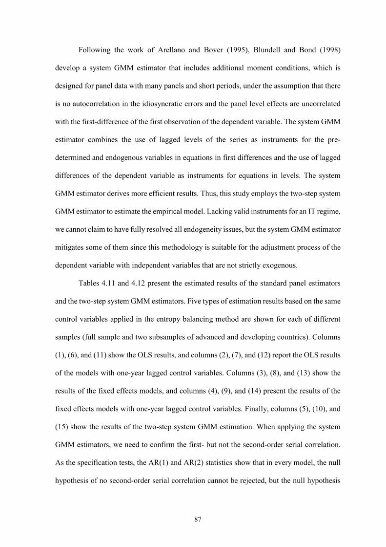
87
Following the work of Arellano and Bover (1995), Blundell and Bond (1998)
develop a system GMM estimator that includes additional moment conditions, which is
designed for panel data with many panels and short periods, under the assumption that there
is no autocorrelation in the idiosyncratic errors and the panel level effects are uncorrelated
with the first-difference of the first observation of the dependent variable. The system GMM
estimator combines the use of lagged levels of the series as instruments for the pre-
determined and endogenous variables in equations in first differences and the use of lagged
differences of the dependent variable as instruments for equations in levels. The system
GMM estimator derives more efficient results. Thus, this study employs the two-step system
GMM estimator to estimate the empirical model. Lacking valid instruments for an IT regime,
we cannot claim to have fully resolved all endogeneity issues, but the system GMM estimator
mitigates some of them since this methodology is suitable for the adjustment process of the
dependent variable with independent variables that are not strictly exogenous.
Tables 4.11 and 4.12 present the estimated results of the standard panel estimators
and the two-step system GMM estimators. Five types of estimation results based on the same
control variables applied in the entropy balancing method are shown for each of different
samples (full sample and two subsamples of advanced and developing countries). Columns
(1), (6), and (11) show the OLS results, and columns (2), (7), and (12) report the OLS results
of the models with one-year lagged control variables. Columns (3), (8), and (13) show the
results of the fixed effects models, and columns (4), (9), and (14) present the results of the
fixed effects models with one-year lagged control variables. Finally, columns (5), (10), and
(15) show the results of the two-step system GMM estimation. When applying the system
GMM estimators, we need to confirm the first- but not the second-order serial correlation.
As the specification tests, the AR(1) and AR(2) statistics show that in every model, the null
hypothesis of no second-order serial correlation cannot be rejected, but the null hypothesis
88
of no first-order serial correlation can be rejected, as required by the specification. In addition,
as the Hansen tests for the exogeneity show that the J-statistic has a p-value greater than 0.10
in all models, we cannot reject the null hypothesis that instruments as a group are exogenous
in the system GMM estimation, as required by the specification.
Our empirical results of the standard panel and system GMM estimation present that
the coefficients on the IT dummy are significantly positive in all models of CBT for the
subsamples of advanced and developing countries, which confirms the empirical results from
the entropy balancing approach that the adoption of IT helps increase the transparency of
central banks in both advanced and developing countries. In addition, our results indicate
that the coefficients on the IT dummy are significantly positive in all models of CBI for
advanced countries, while they are significantly negative in all models of CBI for developing
countries. The IT effects on the independence of central banks are different between
advanced and developing countries: there is a positive IT effect in advanced countries and a
negative IT effect in developing countries. These findings from the standard panel and
system GMM estimation are also consistent with the results of the entropy balancing analysis
in the previous subsection. Thus, our robustness checks confirm the empirical validity of the
estimated results of the entropy balancing method.
4 Conclusion
This study has examined how an IT adoption relates to the credibility of the central bank,
which is captured by its transparency and independence, over 83advanced and developing
countries during the period from 1998 to 2010. This study has applied the entropy balancing
method, which has recently been used to mitigate the self-selection bias although it may
suffer from hidden biases derived from unobserved covariates or factors. Thus, to confirm
the empirical validity of the results of our entropy balancing approach, this study has also
applied the standard panel and dynamic panel methods as alternative methods. Our empirical

89
results have indicated that an IT adoption helps improve central bank transparency in both
advanced and developing countries. Transition of monetary policy frameworks toward the
adoption of an IT regime encourages financial regulators to implement administrative and
institutional reforms such that the central bank provides the general public and financial
markets with relevant information on its policy strategy, decisions, assessments, and their
procedures in an open, clear, and timely manner.
More importantly, our finding has also demonstrated that the IT effects on central
bank independence differ between advanced countries and developing countries, although
central bank independence is generally expected to be granted to central banks to shield them
from short-term political pressures when they fulfill their mandate of ensuring price stability.
In advanced countries, the IT adoption improves central bank independence while it reduces
independence in developing countries. The different IT effects on central bank independence
between advanced and developing countries would be related to different political and
administrative relations between a central bank and government, perhaps including finance
and planning ministries and political institutions, depending on the country’s development
stage. In addition, the negative IT effect on independence in developing countries reflects
the argument in the political economy context that central authorities in developing countries
give parts of the power to a central bank by allowing the central bank to fully control
monetary policy (an IT regime) and to make it more transparent. However, at the same time
central authorities attempt to keep their power by reducing the autonomy or independence
of the central bank.
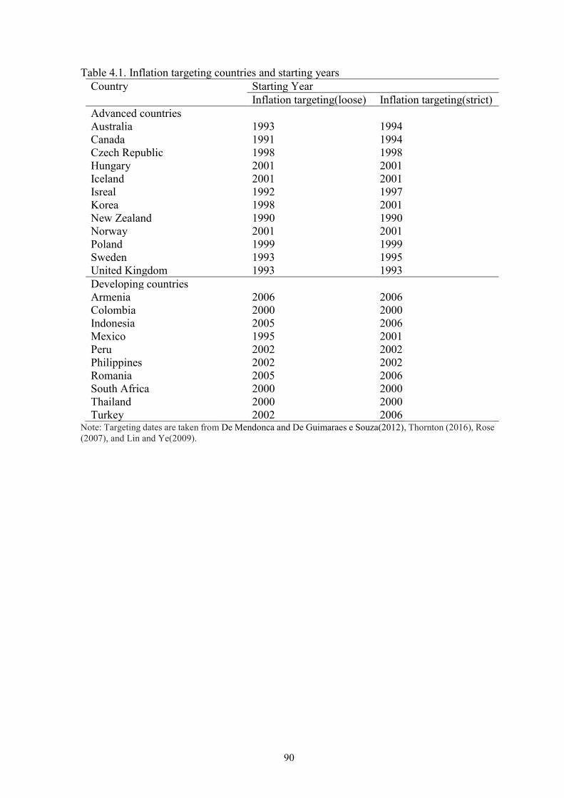
90
Table 4.1. Inflation targeting countries and starting years Country Starting Year Inflation targeting(loose) Inflation targeting(strict) Advanced countries Australia 1993 1994 Canada 1991 1994 Czech Republic 1998 1998 Hungary 2001 2001 Iceland 2001 2001 Isreal 1992 1997 Korea 1998 2001 New Zealand 1990 1990 Norway 2001 2001 Poland 1999 1999 Sweden 1993 1995 United Kingdom 1993 1993 Developing countries Armenia 2006 2006 Colombia 2000 2000 Indonesia 2005 2006 Mexico 1995 2001 Peru 2002 2002 Philippines 2002 2002 Romania 2005 2006 South Africa 2000 2000 Thailand 2000 2000 Turkey 2002 2006
Note: Targeting dates are taken from De Mendonca and De Guimaraes e Souza(2012), Thornton (2016), Rose (2007), and Lin and Ye(2009).

91
Table 4.2. Control group countries Advanced countries Bahama Oman Trinidad and Tobago Barbados Saudi Arbia United Arab Emirates Chile Seychelles United States of America Japan Singapore Developing countries Albania Guyana Nigeria Angola India Papua New Guinca Argentina Iraq Moldova Azerbaijan Jamaica Russia Belarus Jordan Samoa Belize Kenya Sierra Leone Bhutan Kyrgyzstan Solomon Islands Bosnia and Herzegovina Lao PDR Sri Lanka Botswana Lesotho Syria Bulgaria Macedonia Tanzania Cambodia Malawi Tunisia China Malaysia Uganda Croatia Maldives Vanuatu Cuba Mauritius Venezuela El Salvador Mongolia Yamen Fiji Mozambique Zambia Georgia Namibia
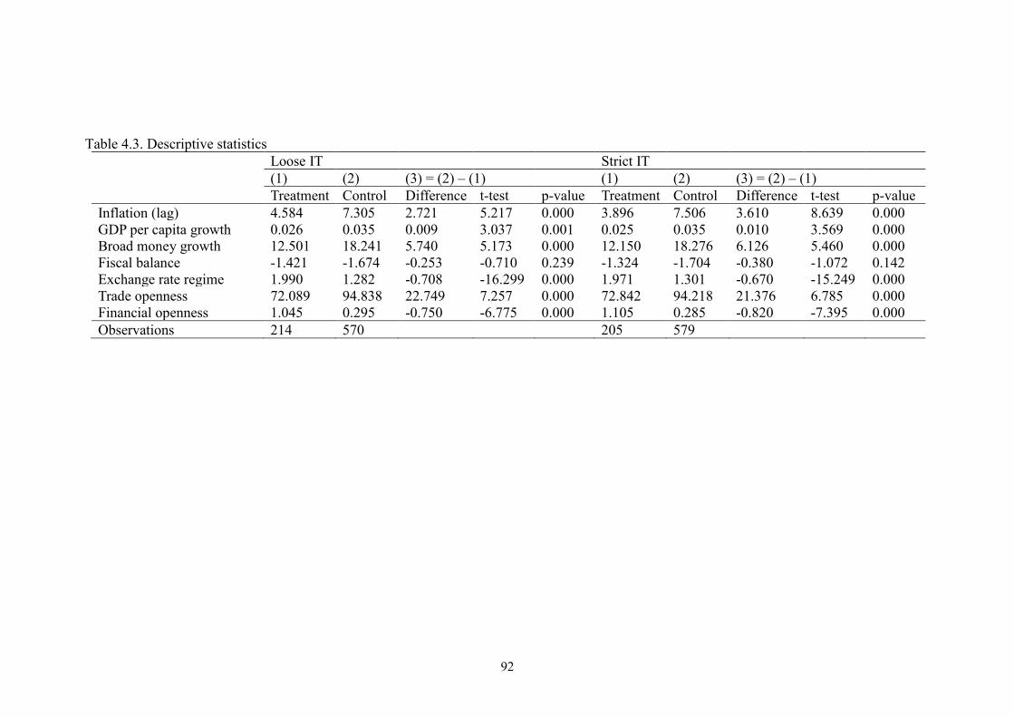
92
Table 4.3. Descriptive statistics
Loose IT Strict IT (1) (2) (3) = (2) – (1) (1) (2) (3) = (2) – (1) Treatment Control Difference t-test p-value Treatment Control Difference t-test p-value Inflation (lag) 4.584 7.305 2.721 5.217 0.000 3.896 7.506 3.610 8.639 0.000 GDP per capita growth 0.026 0.035 0.009 3.037 0.001 0.025 0.035 0.010 3.569 0.000 Broad money growth 12.501 18.241 5.740 5.173 0.000 12.150 18.276 6.126 5.460 0.000 Fiscal balance -1.421 -1.674 -0.253 -0.710 0.239 -1.324 -1.704 -0.380 -1.072 0.142 Exchange rate regime 1.990 1.282 -0.708 -16.299 0.000 1.971 1.301 -0.670 -15.249 0.000 Trade openness 72.089 94.838 22.749 7.257 0.000 72.842 94.218 21.376 6.785 0.000 Financial openness 1.045 0.295 -0.750 -6.775 0.000 1.105 0.285 -0.820 -7.395 0.000 Observations 214 570 205 579
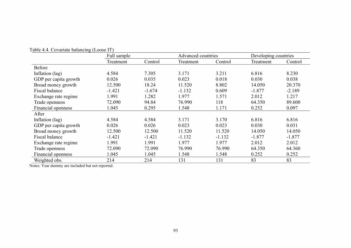
93
Table 4.4. Covariate balancing (Loose IT)
Full sample Advanced countries Developing countries Treatment Control Treatment Control Treatment Control Before Inflation (lag)
4.584
7.305
3.171
3.211
6.816
8.230
GDP per capita growth 0.026 0.035 0.023 0.018 0.030 0.038 Broad money growth 12.500 18.24 11.520 8.802 14.050 20.370 Fiscal balance -1.421 -1.674 -1.132 0.609 -1.877 -2.189 Exchange rate regime 1.991 1.282 1.977 1.571 2.012 1.217 Trade openness 72.090 94.84 76.990 118 64.350 89.600 Financial openness 1.045 0.295 1.548 1.171 0.252 0.097 After Inflation (lag)
4.584
4.584
3.171
3.170
6.816
6.816
GDP per capita growth 0.026 0.026 0.023 0.023 0.030 0.031 Broad money growth 12.500 12.500 11.520 11.520 14.050 14.050 Fiscal balance -1.421 -1.421 -1.132 -1.132 -1.877 -1.877 Exchange rate regime 1.991 1.991 1.977 1.977 2.012 2.012 Trade openness 72.090 72.090 76.990 76.990 64.350 64.360 Financial openness 1.045 1.045 1.548 1.548 0.252 0.252 Weighted obs. 214 214 131 131 83 83
Notes: Year dummy are included but not reported.

94
Table 4.5. Covariate balancing (Strict IT)
Full sample Advanced countries Developing countries Treatment Control Treatment Control Treatment Control Before Inflation (lag)
3.896
7.507
3.155
3.229
5.154
8.477
GDP per capita growth 0.025 0.035 0.022 0.019 0.029 0.039 Broad money growth 12.150 18.280 11.290 9.131 13.610 20.350 Fiscal balance -1.324 -1.704 -1.191 0.648 -1.550 -2.237 Exchange rate regime 1.971 1.301 1.977 1.579 1.961 1.237 Trade openness 72.840 94.220 77.150 117.100 65.530 89.040 Financial openness 1.105 0.285 1.583 1.137 0.294 0.092 After Inflation (lag)
3.896
3.897
3.155
3.155
5.154
5.153
GDP per capita growth 0.025 0.025 0.022 0.022 0.029 0.029 Broad money growth 12.150 12.150 11.290 11.290 13.610 13.610 Fiscal balance -1.324 -1.325 -1.191 -1.190 -1.550 -1.551 Exchange rate regime 1.971 1.971 1.977 1.977 1.961 1.960 Trade openness 72.840 72.840 77.150 77.190 65.530 65.520 Financial openness 1.105 1.105 1.583 1.582 0.294 0.295 Weighted obs. 205 205 129 129 76 76
Notes: Year dummy are included but not reported.
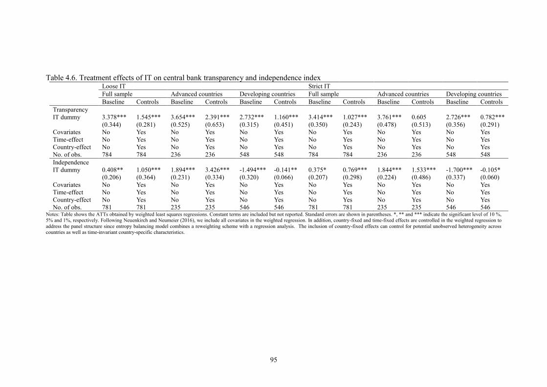
95
Table 4.6. Treatment effects of IT on central bank transparency and independence index
Loose IT Strict IT Full sample Advanced countries Developing countries Full sample Advanced countries Developing countries Baseline Controls Baseline Controls Baseline Controls Baseline Controls Baseline Controls Baseline Controls Transparency IT dummy
3.378*** (0.344)
1.545*** (0.281)
3.654*** (0.525)
2.391*** (0.653)
2.732*** (0.315)
1.160*** (0.451)
3.414*** (0.350)
1.027*** (0.243)
3.761*** (0.478)
0.605 (0.513)
2.726*** (0.356)
0.782*** (0.291)
Covariates No Yes No Yes No Yes No Yes No Yes No Yes Time-effect No Yes No Yes No Yes No Yes No Yes No Yes Country-effect No Yes No Yes No Yes No Yes No Yes No Yes No. of obs. 784 784 236 236 548 548 784 784 236 236 548 548 Independence IT dummy 0.408**
(0.206) 1.050*** (0.364)
1.894*** (0.231)
3.426*** (0.334)
-1.494*** (0.320)
-0.141** (0.066)
0.375* (0.207)
0.769*** (0.298)
1.844*** (0.224)
1.533*** (0.486)
-1.700*** (0.337)
-0.105* (0.060)
Covariates No Yes No Yes No Yes No Yes No Yes No Yes Time-effect No Yes No Yes No Yes No Yes No Yes No Yes Country-effect No Yes No Yes No Yes No Yes No Yes No Yes No. of obs. 781 781 235 235 546 546 781 781 235 235 546 546
Notes: Table shows the ATTs obtained by weighted least squares regressions. Constant terms are included but not reported. Standard errors are shown in parentheses. *, ** and *** indicate the significant level of 10 %, 5% and 1%, respectively. Following Neuenkirch and Neumeier (2016), we include all covariates in the weighted regression. In addition, country-fixed and time-fixed effects are controlled in the weighted regression to address the panel structure since entropy balancing model combines a reweighting scheme with a regression analysis. The inclusion of country-fixed effects can control for potential unobserved heterogeneity across countries as well as time-invariant country-specific characteristics.

96
Table 4.7. Treatment effects of IT on Garriga’s (2016) central bank independence index
Loose IT Strict IT Full Sample Advanced countries Developing countries Full sample Advanced countries Developing
countries Baseline Controls Baseline Controls Baseline Controls Baseline Controls Baseline Controls Baseline Controls Independence IT dummy 0.563***
(0.188) 0.750** (0.345)
1.019*** (0.210)
2.774*** (0.331)
-0.401 (0.339)
-0.560*** (0.158)
0.481** (0.190)
0.498* (0.281)
1.070*** (0.211)
1.181*** (0.422)
-0.725** (0.345)
-0.304** (0.127)
Covariates No Yes No Yes No Yes No Yes No Yes No Yes Time-effect No Yes No Yes No Yes No Yes No Yes No Yes Country-effect No Yes No Yes No Yes No Yes No Yes No Yes No. of obs. 773 773 236 236 537 537 773 773 236 236 537 537
Notes: Table shows the ATTs obtained by weighted least squares regressions. Constant terms are included but not reported. Standard errors are shown in parentheses. *, ** and *** indicate the significant level of 10 %, 5% and 1%, respectively. Following Neuenkirch and Neumeier (2016), we include all covariates in the weighted regression. In addition, country-fixed and time-fixed effects are controlled in the weighted regression to address the panel structure since entropy balancing model combines a reweighting scheme with a regression analysis. The inclusion of country-fixed effects can control for potential unobserved heterogeneity across countries as well as time-invariant country-specific characteristics.
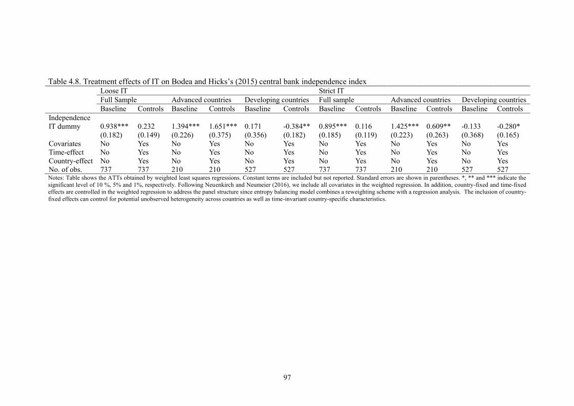
97
Table 4.8. Treatment effects of IT on Bodea and Hicks’s (2015) central bank independence index Loose IT Strict IT Full Sample Advanced countries Developing countries Full sample Advanced countries Developing countries Baseline Controls Baseline Controls Baseline Controls Baseline Controls Baseline Controls Baseline Controls Independence IT dummy 0.938***
(0.182) 0.232 (0.149)
1.394*** (0.226)
1.651*** (0.375)
0.171 (0.356)
-0.384** (0.182)
0.895*** (0.185)
0.116 (0.119)
1.425*** (0.223)
0.609** (0.263)
-0.133 (0.368)
-0.280* (0.165)
Covariates No Yes No Yes No Yes No Yes No Yes No Yes Time-effect No Yes No Yes No Yes No Yes No Yes No Yes Country-effect No Yes No Yes No Yes No Yes No Yes No Yes No. of obs. 737 737 210 210 527 527 737 737 210 210 527 527 Notes: Table shows the ATTs obtained by weighted least squares regressions. Constant terms are included but not reported. Standard errors are shown in parentheses. *, ** and *** indicate the significant level of 10 %, 5% and 1%, respectively. Following Neuenkirch and Neumeier (2016), we include all covariates in the weighted regression. In addition, country-fixed and time-fixed effects are controlled in the weighted regression to address the panel structure since entropy balancing model combines a reweighting scheme with a regression analysis. The inclusion of country-fixed effects can control for potential unobserved heterogeneity across countries as well as time-invariant country-specific characteristics.
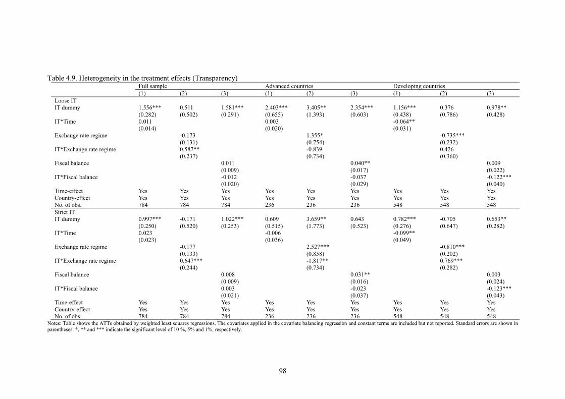
98
Table 4.9. Heterogeneity in the treatment effects (Transparency)
Full sample Advanced countries Developing countries (1) (2) (3) (1) (2) (3) (1) (2) (3) Loose IT IT dummy
1.556*** (0.282)
0.511 (0.502)
1.581*** (0.291)
2.403*** (0.655)
3.405** (1.393)
2.354*** (0.603)
1.156*** (0.438)
0.376 (0.786)
0.978** (0.428)
IT*Time
0.011 (0.014)
0.003 (0.020)
-0.064** (0.031)
Exchange rate regime
-0.173 (0.131)
1.355* (0.754)
-0.735*** (0.232)
IT*Exchange rate regime
0.587** (0.237)
-0.839 (0.734)
0.426 (0.360)
Fiscal balance
0.011 (0.009)
0.040** (0.017)
0.009 (0.022)
IT*Fiscal balance
-0.012 (0.020)
-0.037 (0.029)
-0.122*** (0.040)
Time-effect Yes Yes Yes Yes Yes Yes Yes Yes Yes Country-effect Yes Yes Yes Yes Yes Yes Yes Yes Yes No. of obs. 784 784 784 236 236 236 548 548 548 Strict IT IT dummy
0.997*** (0.250)
-0.171 (0.520)
1.022*** (0.253)
0.609 (0.515)
3.659** (1.773)
0.643 (0.523)
0.782*** (0.276)
-0.705 (0.647)
0.653** (0.282)
IT*Time
0.023 (0.023)
-0.006 (0.036)
-0.099** (0.049)
Exchange rate regime
-0.177 (0.133)
2.527*** (0.858)
-0.810*** (0.202)
IT*Exchange rate regime
0.647*** (0.244)
-1.817** (0.734)
0.769*** (0.282)
Fiscal balance
0.008 (0.009)
0.031** (0.016)
0.003 (0.024)
IT*Fiscal balance
0.003 (0.021)
-0.023 (0.037)
-0.123*** (0.043)
Time-effect Yes Yes Yes Yes Yes Yes Yes Yes Yes Country-effect Yes Yes Yes Yes Yes Yes Yes Yes Yes No. of obs. 784 784 784 236 236 236 548 548 548
Notes: Table shows the ATTs obtained by weighted least squares regressions. The covariates applied in the covariate balancing regression and constant terms are included but not reported. Standard errors are shown in parentheses. *, ** and *** indicate the significant level of 10 %, 5% and 1%, respectively.

99
Table 4.10. Heterogeneity in the treatment effects (Independence) Full sample Advanced countries Developing countries (1) (2) (3) (1) (2) (3) (1) (2) (3) Loose IT IT dummy
1.039*** (0.363)
1.391*** (0.371)
0.938*** (0.309)
3.402*** (0.331)
5.171** (0.768)
3.429*** (0.339)
-0.138** (0.065)
0.203 (0.159)
-0.157** (0.077)
IT*Time
-0.011** (0.005)
-0.006 (0.004)
0.031** (0.014)
Exchange rate regime
0.153** (0.066)
1.592*** (0.229)
0.034 (0.054)
IT*Exchange rate regime
-0.194** (0.097)
-1.442** (0.565)
-0.187* (0.103)
Fiscal balance
-0.005 (0.005)
0.003 (0.005)
0.003 (0.004)
IT*Fiscal balance
0.038** (0.017)
0.004 (0.017)
-0.010 (0.014)
Time-effect Yes Yes Yes Yes Yes Yes Yes Yes Yes Country-effect Yes Yes Yes Yes Yes Yes Yes Yes Yes No. of obs. 781 781 781 235 235 235 546 546 546 Strict IT IT dummy
0.770*** (0.299)
1.229*** (0.343)
0.678*** (0.244)
1.532*** (0.487)
6.751*** (0.802)
1.562*** (0.479)
-0.105* (0.059)
0.204 (0.164)
-0.116* (0.070)
IT*Time
-0.0003 (0.010)
0.002 (0.014)
0.058*** (0.022)
Exchange rate regime
0.183*** (0.069)
3.195*** (0.435)
0.017 (0.050)
IT*Exchange rate regime
-0.248*** (0.095)
-3.106*** (0.420)
-0.160* (0.097)
Fiscal balance
-0.005 (0.005)
0.001 (0.005)
0.002 (0.005)
IT*Fiscal balance
0.041** (0.019)
-0.017 (0.019)
-0.011 (0.019)
Time-effect Yes Yes Yes Yes Yes Yes Yes Yes Yes Country-effect Yes Yes Yes Yes Yes Yes Yes Yes Yes No. of obs. 781 781 781 235 235 235 546 546 546
Notes: Table shows the ATTs obtained by weighted least squares regressions. The covariates applied in the covariate balancing regression and constant terms are included but not reported. Standard errors are shown in parentheses. *, ** and *** indicate the significant level of 10 %, 5% and 1%, respectively.
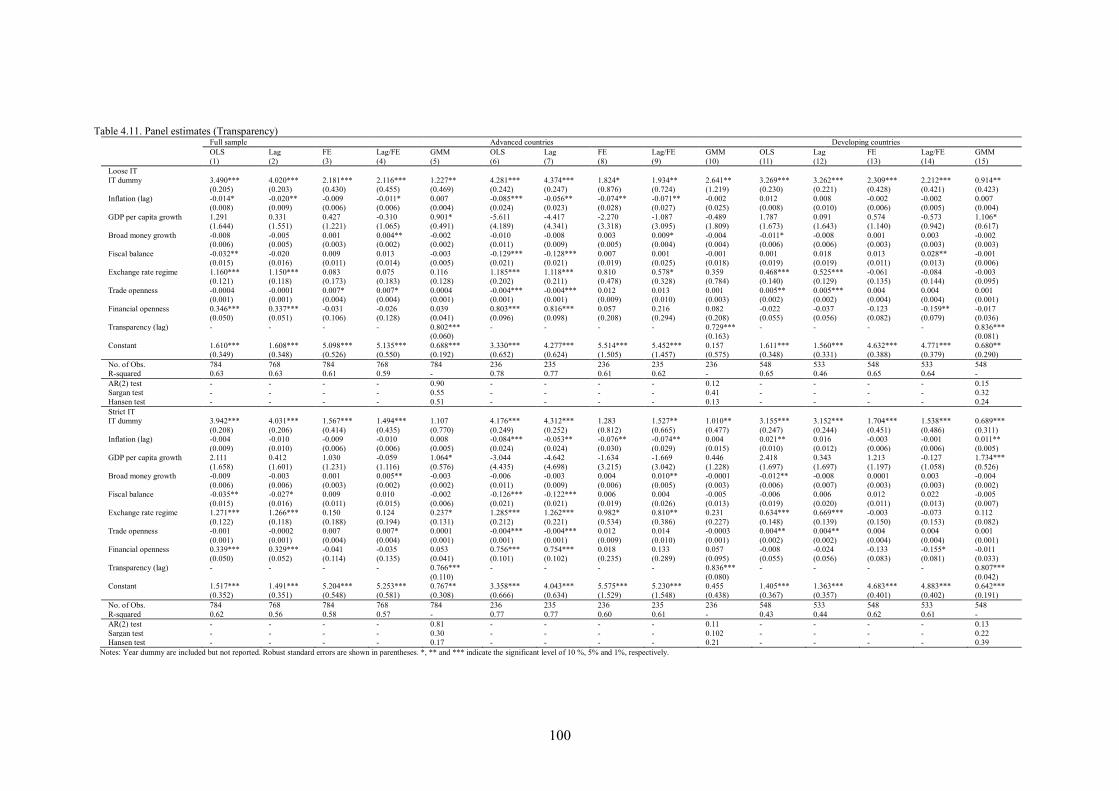
100
Table 4.11. Panel estimates (Transparency)
Full sample Advanced countries Developing countries OLS Lag FE Lag/FE GMM OLS Lag FE Lag/FE GMM OLS Lag FE Lag/FE GMM (1) (2) (3) (4) (5) (6) (7) (8) (9) (10) (11) (12) (13) (14) (15) Loose IT IT dummy
3.490*** (0.205)
4.020*** (0.203)
2.181*** (0.430)
2.116*** (0.455)
1.227** (0.469)
4.281*** (0.242)
4.374*** (0.247)
1.824* (0.876)
1.934** (0.724)
2.641** (1.219)
3.269*** (0.230)
3.262*** (0.221)
2.309*** (0.428)
2.212*** (0.421)
0.914** (0.423)
Inflation (lag)
-0.014* (0.008)
-0.020** (0.009)
-0.009 (0.006)
-0.011* (0.006)
0.007 (0.004)
-0.085*** (0.024)
-0.056** (0.023)
-0.074** (0.028)
-0.071** (0.027)
-0.002 (0.025)
0.012 (0.008)
0.008 (0.010)
-0.002 (0.006)
-0.002 (0.005)
0.007 (0.004)
GDP per capita growth 1.291 (1.644)
0.331 (1.551)
0.427 (1.221)
-0.310 (1.065)
0.901* (0.491)
-5.611 (4.189)
-4.417 (4.341)
-2.270 (3.318)
-1.087 (3.095)
-0.489 (1.809)
1.787 (1.673)
0.091 (1.643)
0.574 (1.140)
-0.573 (0.942)
1.106* (0.617)
Broad money growth -0.008 (0.006)
-0.005 (0.005)
0.001 (0.003)
0.004** (0.002)
-0.002 (0.002)
-0.010 (0.011)
-0.008 (0.009)
0.003 (0.005)
0.009* (0.004)
-0.004 (0.004)
-0.011* (0.006)
-0.008 (0.006)
0.001 (0.003)
0.003 (0.003)
-0.002 (0.003)
Fiscal balance
-0.032** (0.015)
-0.020 (0.016)
0.009 (0.011)
0.013 (0.014)
-0.003 (0.005)
-0.129*** (0.021)
-0.128*** (0.021)
0.007 (0.019)
0.001 (0.025)
-0.001 (0.018)
0.001 (0.019)
0.018 (0.019)
0.013 (0.011)
0.028** (0.013)
-0.001 (0.006)
Exchange rate regime 1.160*** (0.121)
1.150*** (0.118)
0.083 (0.173)
0.075 (0.183)
0.116 (0.128)
1.185*** (0.202)
1.118*** (0.211)
0.810 (0.478)
0.578* (0.328)
0.359 (0.784)
0.468*** (0.140)
0.525*** (0.129)
-0.061 (0.135)
-0.084 (0.144)
-0.003 (0.095)
Trade openness
-0.0004 (0.001)
-0.0001 (0.001)
0.007* (0.004)
0.007* (0.004)
0.0004 (0.001)
-0.004*** (0.001)
-0.004*** (0.001)
0.012 (0.009)
0.013 (0.010)
0.001 (0.003)
0.005** (0.002)
0.005*** (0.002)
0.004 (0.004)
0.004 (0.004)
0.001 (0.001)
Financial openness 0.346*** (0.050)
0.337*** (0.051)
-0.031 (0.106)
-0.026 (0.128)
0.039 (0.041)
0.803*** (0.096)
0.816*** (0.098)
0.057 (0.208)
0.216 (0.294)
0.082 (0.208)
-0.022 (0.055)
-0.037 (0.056)
-0.123 (0.082)
-0.159** (0.079)
-0.017 (0.036)
Transparency (lag) - - - - 0.802*** - - - - 0.729*** - - - - 0.836*** (0.060) (0.163) (0.081) Constant
1.610*** (0.349)
1.608*** (0.348)
5.098*** (0.526)
5.135*** (0.550)
0.688*** (0.192)
3.330*** (0.652)
4.277*** (0.624)
5.514*** (1.505)
5.452*** (1.457)
0.157 (0.575)
1.611*** (0.348)
1.560*** (0.331)
4.632*** (0.388)
4.771*** (0.379)
0.680** (0.290)
No. of Obs. 784 768 784 768 784 236 235 236 235 236 548 533 548 533 548 R-squared 0.63 0.63 0.61 0.59 - 0.78 0.77 0.61 0.62 - 0.65 0.46 0.65 0.64 - AR(2) test - - - - 0.90 - - - - 0.12 - - - - 0.15 Sargan test - - - - 0.55 - - - - 0.41 - - - - 0.32 Hansen test - - - - 0.51 - - - - 0.13 - - - - 0.24 Strict IT IT dummy
3.942*** (0.208)
4.031*** (0.206)
1.567*** (0.414)
1.494*** (0.435)
1.107 (0.770)
4.176*** (0.249)
4.312*** (0.252)
1.283 (0.812)
1.527** (0.665)
1.010** (0.477)
3.155*** (0.247)
3.152*** (0.244)
1.704*** (0.451)
1.538*** (0.486)
0.689*** (0.311)
Inflation (lag)
-0.004 (0.009)
-0.010 (0.010)
-0.009 (0.006)
-0.010 (0.006)
0.008 (0.005)
-0.084*** (0.024)
-0.053** (0.024)
-0.076** (0.030)
-0.074** (0.029)
0.004 (0.015)
0.021** (0.010)
0.016 (0.012)
-0.003 (0.006)
-0.001 (0.006)
0.011** (0.005)
GDP per capita growth 2.111 (1.658)
0.412 (1.601)
1.030 (1.231)
-0.059 (1.116)
1.064* (0.576)
-3.044 (4.435)
-4.642 (4.698)
-1.634 (3.215)
-1.669 (3.042)
0.446 (1.228)
2.418 (1.697)
0.343 (1.697)
1.213 (1.197)
-0.127 (1.058)
1.734*** (0.526)
Broad money growth -0.009 (0.006)
-0.003 (0.006)
0.001 (0.003)
0.005** (0.002)
-0.003 (0.002)
-0.006 (0.011)
-0.003 (0.009)
0.004 (0.006)
0.010** (0.005)
-0.0001 (0.003)
-0.012** (0.006)
-0.008 (0.007)
0.0001 (0.003)
0.003 (0.003)
-0.004 (0.002)
Fiscal balance
-0.035** (0.015)
-0.027* (0.016)
0.009 (0.011)
0.010 (0.015)
-0.002 (0.006)
-0.126*** (0.021)
-0.122*** (0.021)
0.006 (0.019)
0.004 (0.026)
-0.005 (0.013)
-0.006 (0.019)
0.006 (0.020)
0.012 (0.011)
0.022 (0.013)
-0.005 (0.007)
Exchange rate regime 1.271*** (0.122)
1.266*** (0.118)
0.150 (0.188)
0.124 (0.194)
0.237* (0.131)
1.285*** (0.212)
1.262*** (0.221)
0.982* (0.534)
0.810** (0.386)
0.231 (0.227)
0.634*** (0.148)
0.669*** (0.139)
-0.003 (0.150)
-0.073 (0.153)
0.112 (0.082)
Trade openness
-0.001 (0.001)
-0.0002 (0.001)
0.007 (0.004)
0.007* (0.004)
0.0001 (0.001)
-0.004*** (0.001)
-0.004*** (0.001)
0.012 (0.009)
0.014 (0.010)
-0.0003 (0.001)
0.004** (0.002)
0.004** (0.002)
0.004 (0.004)
0.004 (0.004)
0.001 (0.001)
Financial openness 0.339*** (0.050)
0.329*** (0.052)
-0.041 (0.114)
-0.035 (0.135)
0.053 (0.041)
0.756*** (0.101)
0.754*** (0.102)
0.018 (0.235)
0.133 (0.289)
0.057 (0.095)
-0.008 (0.055)
-0.024 (0.056)
-0.133 (0.083)
-0.155* (0.081)
-0.011 (0.033)
Transparency (lag) - - - - 0.766*** (0.110)
- - - - 0.836*** (0.080)
- - - - 0.807*** (0.042)
Constant
1.517*** (0.352)
1.491*** (0.351)
5.204*** (0.548)
5.253*** (0.581)
0.767** (0.308)
3.358*** (0.666)
4.043*** (0.634)
5.575*** (1.529)
5.230*** (1.548)
0.455 (0.438)
1.405*** (0.367)
1.363*** (0.357)
4.683*** (0.401)
4.883*** (0.402)
0.642*** (0.191)
No. of Obs. 784 768 784 768 784 236 235 236 235 236 548 533 548 533 548 R-squared 0.62 0.56 0.58 0.57 - 0.77 0.77 0.60 0.61 - 0.43 0.44 0.62 0.61 - AR(2) test - - - - 0.81 - - - - 0.11 - - - - 0.13 Sargan test - - - - 0.30 - - - - 0.102 - - - - 0.22 Hansen test - - - - 0.17 - - - - 0.21 - - - - 0.39
Notes: Year dummy are included but not reported. Robust standard errors are shown in parentheses. *, ** and *** indicate the significant level of 10 %, 5% and 1%, respectively.
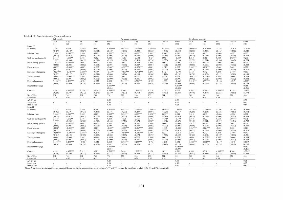
101
Table 4.12. Panel estimates (Independence)
Full sample Advanced countries Developing countries OLS Lag FE Lag/FE GMM OLS Lag FE Lag/FE GMM OLS Lag FE Lag/FE GMM (1) (2) (3) (4) (5) (6) (7) (8) (9) (10) (11) (12) (13) (14) (15) Loose IT IT dummy
0.297 (0.189)
0.295 (0.187)
0.896* (0.527)
0.997 (0.614)
0.501*** (0.189)
2.042*** (0.238)
2.109*** (0.238)
3.347*** (0.565)
3.478*** (0.587)
1.007** (0.358)
-0.859*** (0.255)
-0.803*** (0.256)
-0.156 (0.165)
-0.282* (0.162)
-1.012* (0.545)
Inflation (lag)
0.040*** (0.011)
0.049*** (0.012)
0.003 (0.004)
0.002 (0.006)
0.006** (0.003)
0.095*** (0.025)
0.102*** (0.029)
0.031*** (0.009)
0.340*** (0.011)
0.016 (0.023)
0.014 (0.011)
0.017 (0.013)
-0.003 (0.003)
-0.003 (0.005)
0.003 (0.005)
GDP per capita growth 3.315* (1.997)
4.096** (1.906)
0.345 (0.659)
0.382 (0.633)
0.010 (0.378)
-4.317 (3.472)
-3.504 (3.418)
-0.427 (0.736)
0.095 (0.535)
-0.449 (1.130)
1.210 (2.132)
2.185 (2.084)
0.703 (0.546)
1.038** (0.447)
0.290 (0.774)
Broad money growth 0.017*** (0.005)
0.015*** (0.005)
-0.001 (0.002)
0.002 (0.002)
0.002 (0.001)
0.001 (0.008)
-0.003 (0.007)
0.002 (0.001)
0.002 (0.001)
-0.001 (0.002)
0.012** (0.006)
0.012** (0.006)
-0.002 (0.002)
0.002 (0.002)
0.003 (0.003)
Fiscal balance
-0.033* (0.017)
-0.035** (0.017)
-0.003 (0.006)
-0.002 (0.005)
-0.007* (0.004)
-0.065*** (0.020)
-0.070*** (0.020)
-0.001 (0.003)
-0.010 (0.007)
0.002 (0.008)
0.062*** (0.022)
0.058*** (0.022)
-0.001 (0.009)
0.002 (0.006)
0.021 (0.017)
Exchange rate regime -0.537*** (0.127)
-0.523*** (0.127)
0.220** (0.107)
0.179* (0.099)
-0.159* (0.088)
-0.697*** (0.174)
-0.714*** (0.169)
0.295 (0.200)
0.112 (0.119)
-0.104 (0.192)
0.168 (0.170)
0.172 (0.168)
0.173 (0.112)
0.168* (0.010)
0.189 (0.188)
Trade openness
-0.004*** (0.001)
-0.004*** (0.001)
0.002 (0.002)
0.0004 (0.002)
0.0002 (0.0004)
0.001 (0.001)
0.0002 (0.001)
0.001 (0.002)
-0.001 (0.002)
0.001 (0.001)
-0.005*** (0.002)
-0.005** (0.002)
0.002 (0.002)
0.0004 (0.002)
-0.003 (0.004)
Financial openness 0.146*** (0.049)
0.160*** (0.050)
-0.114 (0.128)
-0.037 (0.127)
0.004 (0.022)
0.319*** (0.074)
0.306*** (0.070)
-0.122 (0.079)
-0.060 (0.061)
-0.002 (0.069)
0.314*** (0.066)
0.331*** (0.066)
-0.148 (0.153)
-0.045 (0.161)
0.180* (0.104)
Independence (lag) - - - - 0.890*** (0.034)
- - - - 0.876** (0.024)
- - - - 0.385 (0.266)
Constant
4.401*** (0.358)
4.446*** (0.395)
3.770*** (0.312)
3.930*** (0.275)
0.518*** (0.180)
2.106*** (0.577)
2.864*** (0.514)
1.119* (0.590)
1.378*** (0.467)
0.009 (0.284)
4.647*** (0.449)
4.708*** (0.497)
4.593*** (0.235)
4.758*** (0.160)
3.117* (1.572)
No. of Obs. 781 765 781 765 776 235 234 235 234 233 546 531 546 531 543 R-squared 0.10 0.10 0.18 0.17 - 0.34 0.35 0.71 0.71 - 0.10 0.11 0.13 0.11 - AR (2) test - - - - 0.18 - - - - 0.40 - - - - 0.38 Sargan test - - - - 0.81 - - - - 0.77 - - - - 0.85 Hansen test - - - - 0.30 - - - - 0.28 - - - - 0.84 Strict IT IT dummy
0.215 (0.193)
0.226 (0.191)
0.650 (0.431)
0.706 (0.485)
0.476*** (0.176)
1.981*** (0.237)
2.049*** (0.237)
2.504*** (0.804)
2.684*** (0.728)
1.116** (0.517)
-1.124*** (0.258)
-1.058*** (0.263)
-0.204 (0.126)
-0.278* (0.157)
-0.999* (0.552)
Inflation (lag)
0.040*** (0.011)
0.049*** (0.012)
0.002 (0.005)
0.003 (0.006)
0.007** (0.003)
0.095*** (0.025)
0.103*** (0.030)
0.028*** (0.009)
0.033** (0.014)
0.011 (0.026)
0.010 (0.011)
0.013 (0.012)
-0.004 (0.004)
-0.004 (0.005)
0.002 (0.005)
GDP per capita growth 3.358* (1.993)
4.092** (1.902)
0.595 (0.588)
0.499 (0.610)
0.154 (0.402)
-3.031 (3.570)
-3.515 (3.674)
0.796 (1.287)
-0.941* (0.481)
-0.570 (1.074)
0.954 (2.142)
2.022 (2.094)
0.653 (0.519)
0.987** (0.424)
0.075 (0.735)
Broad money growth 0.017*** (0.005)
0.015*** (0.005)
-0.001 (0.002)
0.003* (0.002)
0.002 (0.001)
0.001 (0.008)
-0.001 (0.007)
0.005* (0.002)
0.004** (0.002)
-0.003 (0.003)
0.012** (0.006)
0.011* (0.006)
-0.002 (0.002)
0.002 (0.002)
0.004 (0.003)
Fiscal balance
-0.032* (0.017)
-0.035** (0.017)
-0.003 (0.006)
0.001 (0.006)
-0.007* (0.004)
-0.063*** (0.020)
-0.067*** (0.020)
-0.003 (0.003)
-0.005 (0.005)
-0.003 (0.013)
0.067*** (0.022)
0.064*** (0.022)
-0.001 (0.009)
0.003 (0.006)
0.024 (0.018)
Exchange rate regime -0.506*** (0.124)
-0.496*** (0.123)
0.248** (0.117)
0.201* (0.105)
-0.139* (0.082)
-0.648*** (0.175)
-0.641*** (0.174)
0.597 (0.395)
0.531 (0.322)
-0.214 (0.322)
0.208 (0.162)
0.212 (0.161)
0.171 (0.109)
0.169* (0.100)
0.147 (0.201)
Trade openness
-0.004*** (0.001)
-0.004*** (0.001)
0.002 (0.002)
0.0004 (0.002)
0.0001 (0.0004)
0.0003 (0.001)
0.0001 (0.001)
0.0001 (0.002)
0.001 (0.003)
0.001 (0.002)
-0.006*** (0.002)
-0.005** (0.002)
0.002 (0.002)
0.0004 (0.002)
-0.004 (0.004)
Financial openness 0.150*** (0.050)
0.163*** (0.050)
-0.118 (0.128)
-0.041 (0.128)
0.005 (0.022)
0.296*** (0.076)
0.277*** (0.073)
-0.196 (0.127)
-0.207 (0.112)
0.032 (0.116)
0.322*** (0.066)
0.338*** (0.066)
-0.147 (0.153)
-0.046 (0.162)
0.184* (0.106)
Independence (lag) - - - - 0.890*** (0.034)
- - - - 0.786*** (0.093)
- - - - 0.352 (0.261)
Constant
4.392*** (0.359)
4.437*** (0.396)
3.812*** (0.321)
3.985*** (0.277)
0.503*** (0.173)
2.658*** (0.505)
2.902*** (0.523)
1.176 (0.731)
1.015* (0.557)
0.386 (0.552)
4.668*** (0.441)
4.710*** (0.485)
4.613*** (0.235)
4.764*** (0.161)
3.326** (1.583)
No. of Obs. 781 765 781 765 776 235 234 235 234 233 546 531 546 531 543 R-squared 0.10 0.10 0.16 0.15 - 0.33 0.34 0.57 0.58 - 0.10 0.1 0.13 0.11 - AR (2) test - - - - 0.19 - - - - 0.37 - - - - 0.36 Sargan test - - - - 0.81 - - - - 0.19 - - - - 0.87 Hansen test - - - - 0.27 - - - - 0.17 - - - - 0.87
Notes: Year dummy are included but not reported. Robust standard errors are shown in parentheses. *, ** and *** indicate the significant level of 10 %, 5% and 1%, respectively.
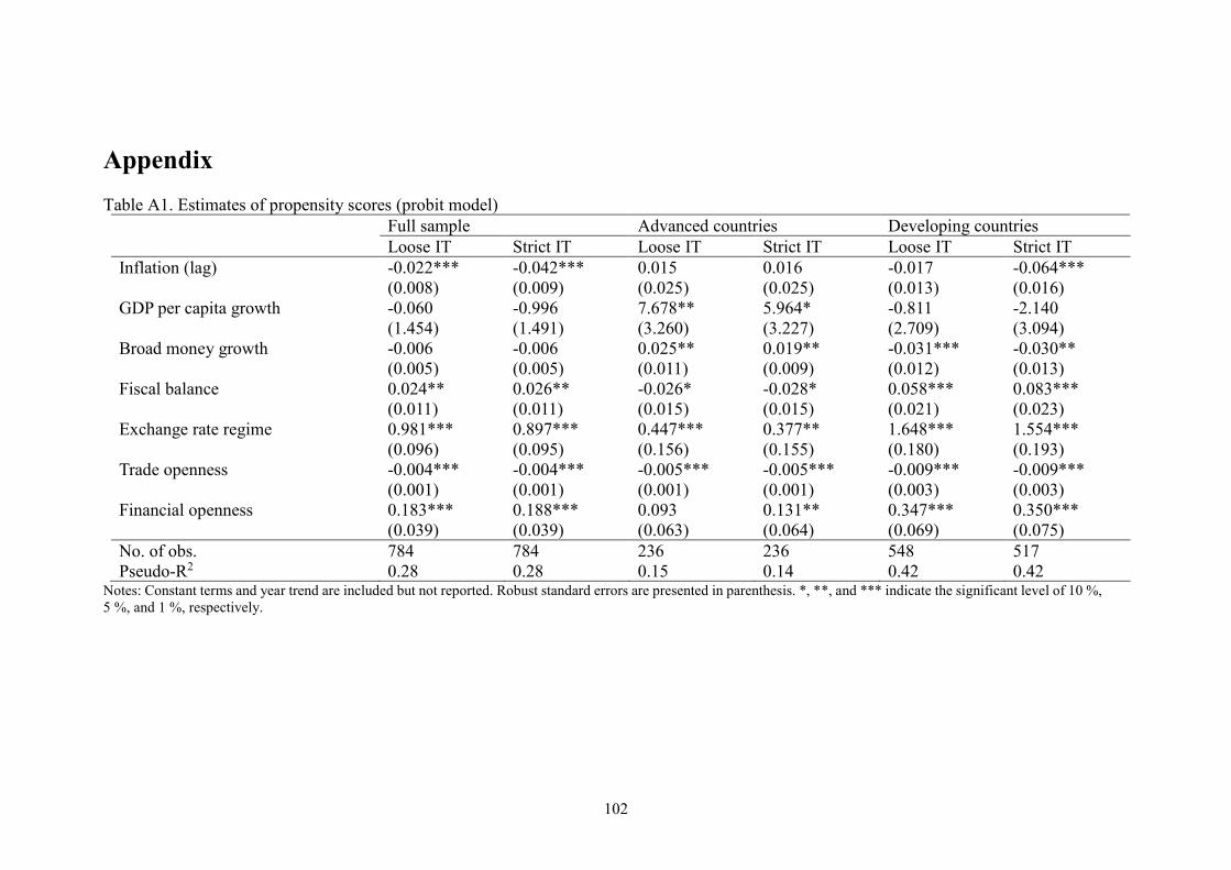
102
Appendix Table A1. Estimates of propensity scores (probit model)
Full sample Advanced countries Developing countries Loose IT Strict IT Loose IT Strict IT Loose IT Strict IT Inflation (lag) -0.022***
(0.008) -0.042*** (0.009)
0.015 (0.025)
0.016 (0.025)
-0.017 (0.013)
-0.064*** (0.016)
GDP per capita growth -0.060 (1.454)
-0.996 (1.491)
7.678** (3.260)
5.964* (3.227)
-0.811 (2.709)
-2.140 (3.094)
Broad money growth -0.006 (0.005)
-0.006 (0.005)
0.025** (0.011)
0.019** (0.009)
-0.031*** (0.012)
-0.030** (0.013)
Fiscal balance 0.024** (0.011)
0.026** (0.011)
-0.026* (0.015)
-0.028* (0.015)
0.058*** (0.021)
0.083*** (0.023)
Exchange rate regime 0.981*** (0.096)
0.897*** (0.095)
0.447*** (0.156)
0.377** (0.155)
1.648*** (0.180)
1.554*** (0.193)
Trade openness -0.004*** (0.001)
-0.004*** (0.001)
-0.005*** (0.001)
-0.005*** (0.001)
-0.009*** (0.003)
-0.009*** (0.003)
Financial openness 0.183*** (0.039)
0.188*** (0.039)
0.093 (0.063)
0.131** (0.064)
0.347*** (0.069)
0.350*** (0.075)
No. of obs. 784 784 236 236 548 517 Pseudo-R2 0.28 0.28 0.15 0.14 0.42 0.42
Notes: Constant terms and year trend are included but not reported. Robust standard errors are presented in parenthesis. *, **, and *** indicate the significant level of 10 %, 5 %, and 1 %, respectively.
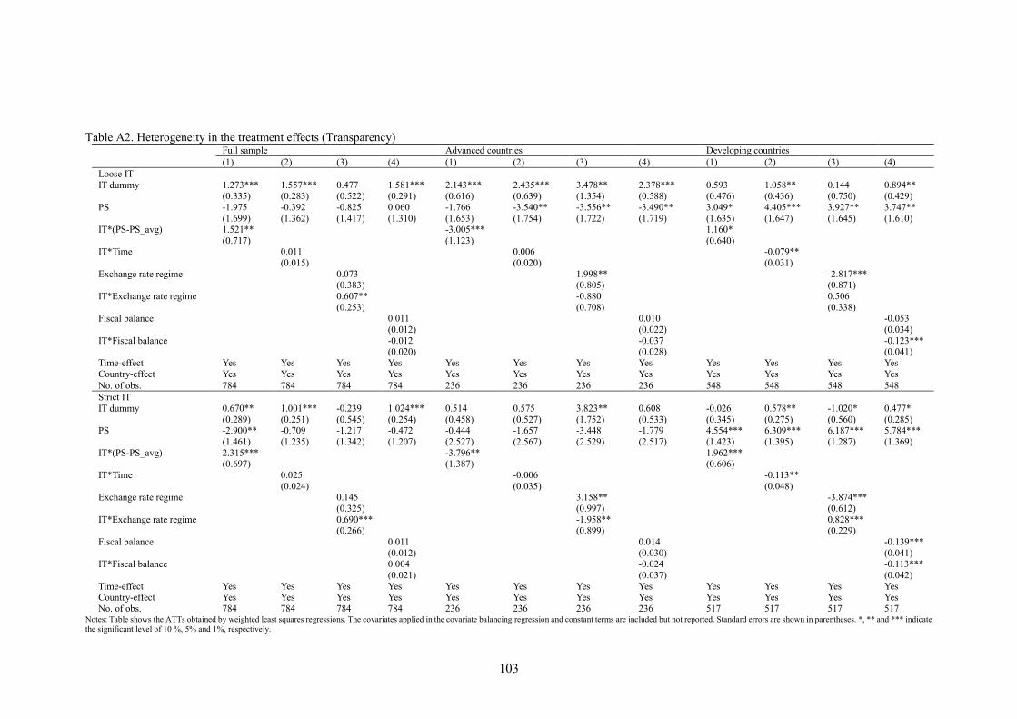
103
Table A2. Heterogeneity in the treatment effects (Transparency)
Full sample Advanced countries Developing countries (1) (2) (3) (4) (1) (2) (3) (4) (1) (2) (3) (4) Loose IT IT dummy
1.273*** (0.335)
1.557*** (0.283)
0.477 (0.522)
1.581*** (0.291)
2.143*** (0.616)
2.435*** (0.639)
3.478** (1.354)
2.378*** (0.588)
0.593 (0.476)
1.058** (0.436)
0.144 (0.750)
0.894** (0.429)
PS -1.975 (1.699)
-0.392 (1.362)
-0.825 (1.417)
0.060 (1.310)
-1.766 (1.653)
-3.540** (1.754)
-3.556** (1.722)
-3.490** (1.719)
3.049* (1.635)
4.405*** (1.647)
3.927** (1.645)
3.747** (1.610)
IT*(PS-PS_avg) 1.521** (0.717)
-3.005*** (1.123)
1.160* (0.640)
IT*Time
0.011 (0.015)
0.006 (0.020)
-0.079** (0.031)
Exchange rate regime
0.073 (0.383)
1.998** (0.805)
-2.817*** (0.871)
IT*Exchange rate regime
0.607** (0.253)
-0.880 (0.708)
0.506 (0.338)
Fiscal balance
0.011 (0.012)
0.010 (0.022)
-0.053 (0.034)
IT*Fiscal balance
-0.012 (0.020)
-0.037 (0.028)
-0.123*** (0.041)
Time-effect Yes Yes Yes Yes Yes Yes Yes Yes Yes Yes Yes Yes Country-effect Yes Yes Yes Yes Yes Yes Yes Yes Yes Yes Yes Yes No. of obs. 784 784 784 784 236 236 236 236 548 548 548 548 Strict IT IT dummy
0.670** (0.289)
1.001*** (0.251)
-0.239 (0.545)
1.024*** (0.254)
0.514 (0.458)
0.575 (0.527)
3.823** (1.752)
0.608 (0.533)
-0.026 (0.345)
0.578** (0.275)
-1.020* (0.560)
0.477* (0.285)
PS -2.900** (1.461)
-0.709 (1.235)
-1.217 (1.342)
-0.472 (1.207)
-0.444 (2.527)
-1.657 (2.567)
-3.448 (2.529)
-1.779 (2.517)
4.554*** (1.423)
6.309*** (1.395)
6.187*** (1.287)
5.784*** (1.369)
IT*(PS-PS_avg) 2.315*** (0.697)
-3.796** (1.387)
1.962*** (0.606)
IT*Time
0.025 (0.024)
-0.006 (0.035)
-0.113** (0.048)
Exchange rate regime
0.145 (0.325)
3.158** (0.997)
-3.874*** (0.612)
IT*Exchange rate regime
0.690*** (0.266)
-1.958** (0.899)
0.828*** (0.229)
Fiscal balance
0.011 (0.012)
0.014 (0.030)
-0.139*** (0.041)
IT*Fiscal balance
0.004 (0.021)
-0.024 (0.037)
-0.113*** (0.042)
Time-effect Yes Yes Yes Yes Yes Yes Yes Yes Yes Yes Yes Yes Country-effect Yes Yes Yes Yes Yes Yes Yes Yes Yes Yes Yes Yes No. of obs. 784 784 784 784 236 236 236 236 517 517 517 517
Notes: Table shows the ATTs obtained by weighted least squares regressions. The covariates applied in the covariate balancing regression and constant terms are included but not reported. Standard errors are shown in parentheses. *, ** and *** indicate the significant level of 10 %, 5% and 1%, respectively.
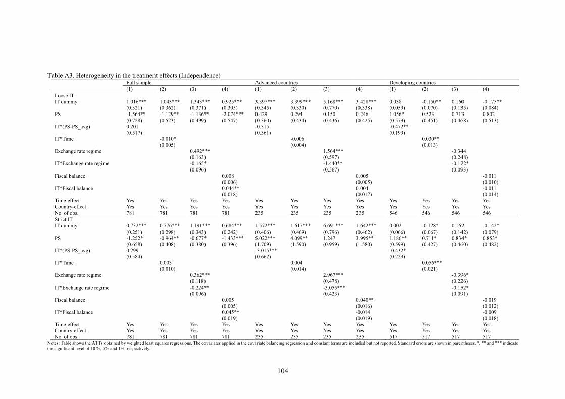
104
Table A3. Heterogeneity in the treatment effects (Independence) Full sample Advanced countries Developing countries (1) (2) (3) (4) (1) (2) (3) (4) (1) (2) (3) (4) Loose IT IT dummy
1.016*** (0.321)
1.043*** (0.362)
1.343*** (0.371)
0.925*** (0.305)
3.397*** (0.345)
3.399*** (0.330)
5.168*** (0.770)
3.428*** (0.338)
0.038 (0.059)
-0.150** (0.070)
0.160 (0.135)
-0.175** (0.084)
PS -1.564** (0.728)
-1.129** (0.523)
-1.136** (0.499)
-2.074*** (0.547)
0.429 (0.360)
0.294 (0.434)
0.150 (0.436)
0.246 (0.425)
1.056* (0.579)
0.523 (0.451)
0.713 (0.468)
0.802 (0.513)
IT*(PS-PS_avg) 0.201 (0.517)
-0.315 (0.361)
-0.472** (0.199)
IT*Time
-0.010* (0.005)
-0.006 (0.004)
0.030** (0.013)
Exchange rate regime
0.492*** (0.163)
1.564*** (0.597)
-0.344 (0.248)
IT*Exchange rate regime
-0.165* (0.096)
-1.440** (0.567)
-0.172* (0.093)
Fiscal balance
0.008 (0.006)
0.005 (0.005)
-0.011 (0.010)
IT*Fiscal balance
0.044** (0.018)
0.004 (0.017)
-0.011 (0.014)
Time-effect Yes Yes Yes Yes Yes Yes Yes Yes Yes Yes Yes Yes Country-effect Yes Yes Yes Yes Yes Yes Yes Yes Yes Yes Yes Yes No. of obs. 781 781 781 781 235 235 235 235 546 546 546 546 Strict IT IT dummy
0.732*** (0.251)
0.776*** (0.298)
1.191*** (0.343)
0.684*** (0.242)
1.572*** (0.406)
1.617*** (0.469)
6.691*** (0.796)
1.642*** (0.462)
0.002 (0.066)
-0.128* (0.067)
0.162 (0.142)
-0.142* (0.079)
PS -1.252* (0.658)
-0.964** (0.408)
-0.677* (0.380)
-1.433*** (0.396)
5.022*** (1.709)
4.099** (1.590)
1.247 (0.959)
3.995** (1.580)
1.186** (0.599)
0.711* (0.427)
0.834* (0.460)
0.853* (0.482)
IT*(PS-PS_avg) 0.299 (0.584)
-3.015*** (0.662)
-0.432* (0.229)
IT*Time
0.003 (0.010)
0.004 (0.014)
0.056*** (0.021)
Exchange rate regime
0.362*** (0.118)
2.967*** (0.478)
-0.396* (0.226)
IT*Exchange rate regime
-0.224** (0.096)
-3.055*** (0.423)
-0.152* (0.091)
Fiscal balance
0.005 (0.005)
0.040** (0.016)
-0.019 (0.012)
IT*Fiscal balance
0.045** (0.019)
-0.014 (0.019)
-0.009 (0.018)
Time-effect Yes Yes Yes Yes Yes Yes Yes Yes Yes Yes Yes Yes Country-effect Yes Yes Yes Yes Yes Yes Yes Yes Yes Yes Yes Yes No. of obs. 781 781 781 781 235 235 235 235 517 517 517 517
Notes: Table shows the ATTs obtained by weighted least squares regressions. The covariates applied in the covariate balancing regression and constant terms are included but not reported. Standard errors are shown in parentheses. *, ** and *** indicate the significant level of 10 %, 5% and 1%, respectively.
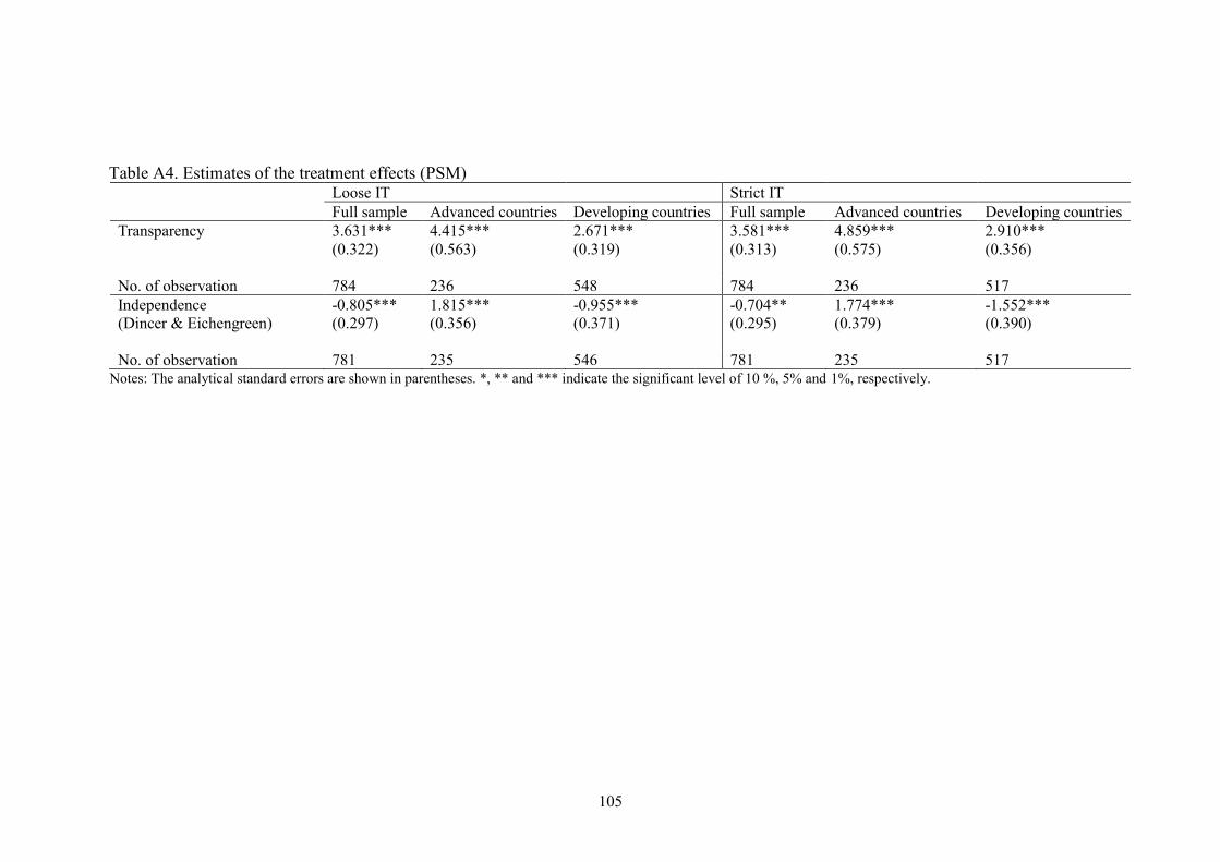
105
Table A4. Estimates of the treatment effects (PSM)
Loose IT Strict IT Full sample Advanced countries Developing countries Full sample Advanced countries Developing countries Transparency 3.631***
(0.322) 4.415*** (0.563)
2.671*** (0.319)
3.581*** (0.313)
4.859*** (0.575)
2.910*** (0.356)
No. of observation 784 236 548 784 236 517 Independence (Dincer & Eichengreen)
-0.805*** (0.297)
1.815*** (0.356)
-0.955*** (0.371)
-0.704** (0.295)
1.774*** (0.379)
-1.552*** (0.390)
No. of observation 781 235 546 781 235 517 Notes: The analytical standard errors are shown in parentheses. *, ** and *** indicate the significant level of 10 %, 5% and 1%, respectively.
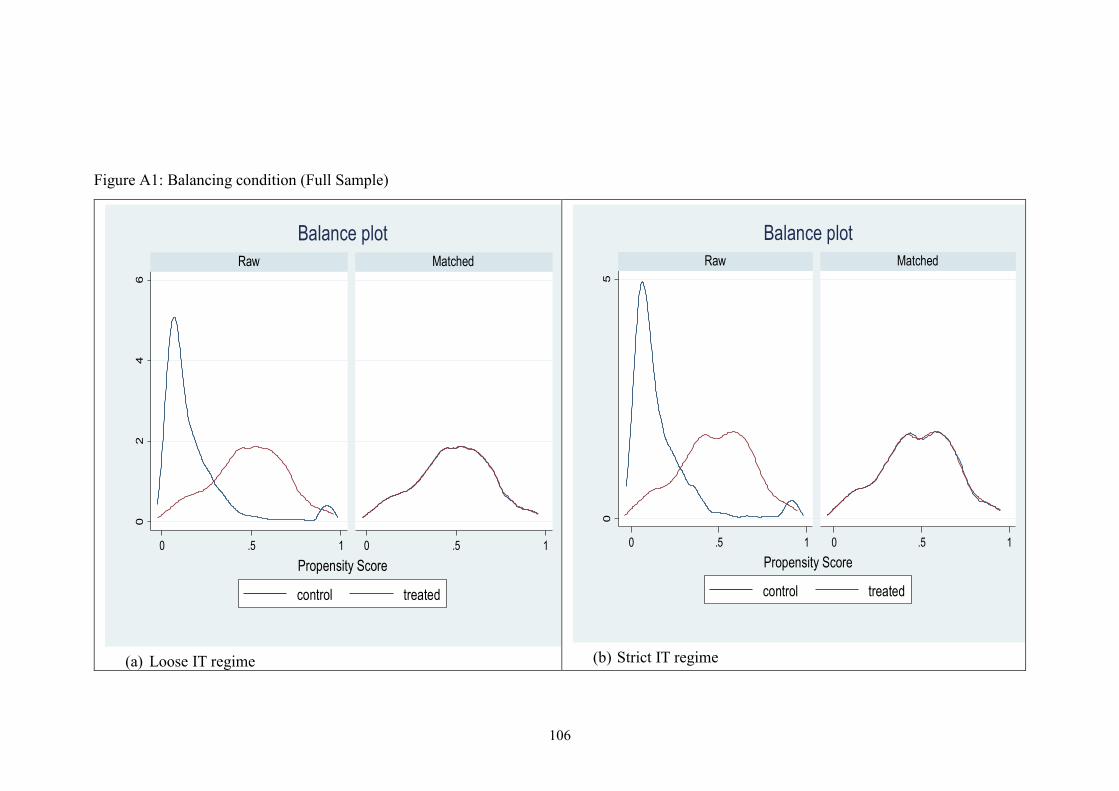
106
Figure A1: Balancing condition (Full Sample)
(a) Loose IT regime
(b) Strict IT regime
02
46
0 .5 1 0 .5 1
Raw Matched
control treated
Den
sity
Propensity Score
Balance plot
05
0 .5 1 0 .5 1
Raw Matched
control treated
Den
sity
Propensity Score
Balance plot
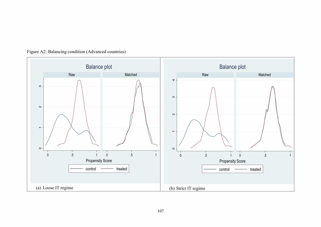
107
Figure A2: Balancing condition (Advanced countries)
(a) Loose IT regime
(b) Strict IT regime
01
23
0 .5 1 0 .5 1
Raw Matched
control treated
Den
sity
Propensity Score
Balance plot
01
23
4
0 .5 1 0 .5 1
Raw Matched
control treated
Den
sity
Propensity Score
Balance plot
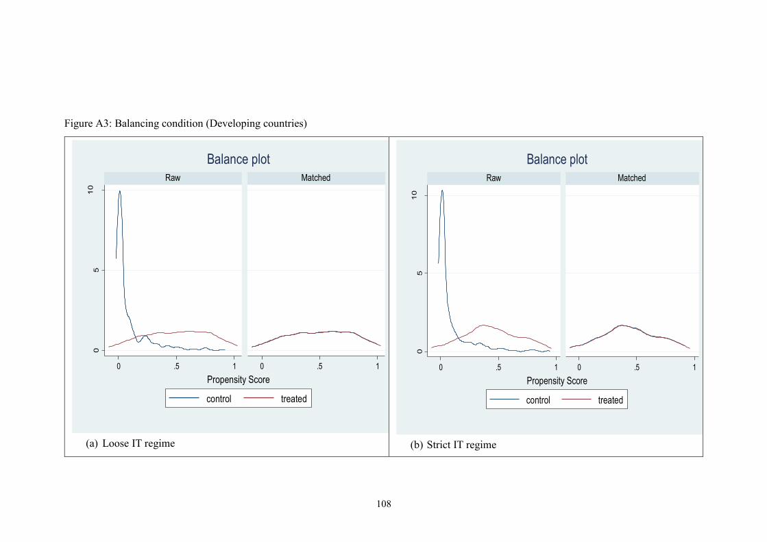
108
Figure A3: Balancing condition (Developing countries)
(a) Loose IT regime
(b) Strict IT regime
05
10
0 .5 1 0 .5 1
Raw Matched
control treated
Den
sity
Propensity Score
Balance plot
05
10
0 .5 1 0 .5 1
Raw Matched
control treated
Den
sity
Propensity Score
Balance plot
109
Chapter 5
Conclusion
Since an IT regime has been widely adopted not only in advanced countries but also in
developing countries as a monetary policy strategy, the policy makers and researches
discusses the beneficial effects of the IT adoption on macroeconomic performance
theoretically and empirically. Many empirical studies mainly examine the impacts of an IT
regime on inflation, inflation volatility, and output volatility applying different
methodologies including the DID and PSM methods. Generally, they suggest that an IT
regime helps improve macroeconomic performance with low inflation, and the stability of
inflation and output in developing countries while there is no clear evidence of a beneficial
IT effect in advanced countries. However, the IT adoption might have several effects in
various contexts. Thus, this dissertation has attempted to examine how an IT regime is
related to domestic economy, external economy, and the institutional structure.
The first study has investigated the IT effects on income velocity which is related to
domestic economy, over 84 developing countries from the period 1990 to 2013. Although
an IT regime has become popular even in developing countries, many developing countries
are still adopting monetary aggregates targeting due to unmatured money and financial
markets. However, monetary aggregates targeting is often ineffective with the frequently
failure of macroeconomic stability. Unstable income velocity is one of the main reasons for
ineffective monetary aggregates targeting (Mishkin, 2006). According to Park (1970),
income velocity is more volatile in developing countries than in advanced countries. Thus,
stability of income velocity is crucial to achieve macroeconomic stability under monetary
aggregates targeting. Taylor (2000) highlights that monetary targeting and inflation targeting
can coexist and monetary aggregates would be an appropriate instrument to achieve inflation
target in developing countries due to real interest rate uncertainty. If an IT regime helps
110
stabilize income velocity, monetary authorities can justify monetary aggregates targeting as
an effective policy measure under an IT regime. Thus, the first study has attempted to
examine the relationship between an IT regime and income velocity in developing countries.
The second study has examined the impacts of an IT regime on exchange market
pressure which is related to external economy, over 101 developing countries from the period
1990 to 2014. Developing countries have often experienced foreign exchange market
instability. Since foreign exchange markets are closely related to external conditions of an
economy, foreign exchange market turmoil often induce the instability of external economy
so that a sound monetary policy arrangement is important to absorb foreign exchange market
pressures for their macroeconomic stability. If IT regime helps stabilize the exchange market
pressures, policy makers will achieve the favorable external conditions and macroeconomic
stability under an IT regime. Thus, the second study has attempted to investigate the
relationship between an IT regime and exchange market pressure in developing countries.
The third study has analyzed the impacts of an IT regime on the credibility of the
central bank which is captured by its transparency and independence, over 83 advanced and
developing countries during the period from 1998 to 2010. Achieving macroeconomic and
financial stability requires monetary policy credibility, which is closely related to
institutional structure and their reforms so that many countries have been implementing the
institutional reforms to achieve credibility. In addition, Eijffinger and Hoeberichts (2002)
and Eijffinger et al. (2006) argue that central banks` monetary policy credibility is closely
related to institutional reforms on (i) independence from the government and (ii)
transparency to the public. At the same time, the IT adoption is one of the crucial monetary
policy frameworks, which is expected to increase the monetary policy credibility. If an IT
regime induces central bank credibility, policy makers will achieve favorable
macroeconomic outcomes under an IT regime. Thus, the third study has attempted to
111
investigate the relationship between an IT regime and credibility of the central banks in
advanced and developing countries.
This dissertation has applied the propensity score matching (PSM) and entropy
balancing methods to discuss three contents: the first content is to examine the impact of an
IT regime on income velocity volatility in developing countries, the second content is to
examine the impact of an IT regime on exchange market pressure in developing countries,
and the third content is to investigate the impact of an IT regime on the credibility of the
central bank in advanced and developing countries. The first study has applied the PSM
method to examine whether IT helps stabilize income velocity variability. The PSM method
has commonly been used to eliminate self-selection bias, although it may suffer from issues
related to small samples as well as hidden biases derived from unobserved covariates or
factors (Pearl, 2000).
To confirm the empirical validity of our PSM results, this study has also applied
another method widely used in IT-related studies, the DID method. The empirical results of
both methods have indicated that IT would help stabilize income velocity in developing
countries. Thus, our findings have shown clear support for Taylor’s (2000) argument that
monetary authorities in developing economies would prefer using monetary policy rule with
monetary aggregates to achieve inflation targets under stable income velocity. In addition,
our empirical results regarding IT effects on income velocity have highlighted that monetary
authorities can pursue monetary aggregates as an effective policy measure under an IT
regime. Moreover, our decomposition analysis of income velocity variability has provided
evidences that IT lessens volatilities of inflation, real output growth, and money growth.
Furthermore, our analysis of heterogeneous effects has revealed that an IT regime would be
effective in reducing income velocity volatility under the favorable preconditions of IT
adoption and floating exchange rate regime application. The time length also influences the
112
effectiveness of an IT regime, and IT is likely to become more effective in lowering income
velocity volatility over time.
The second study has also applied the PSM method to examine whether an IT regime
helps stabilize EMP and its two components. The empirical results have indicated that an IT
regime would help stabilize EMP. In addition, our analysis has provided evidences that an
IT regime lessens volatility of changes in international reserves, while our results show no
clear evidence that an IT regime affects exchange rate variability. These findings suggest
that the policy commitment to an IT regime improves the credibility of monetary policy
conduct. Under an IT regime, central banks would not be required to intervene in the foreign
exchange market. More interestingly, our findings have also shown that an IT regime is more
beneficial for middle-income developing countries rather than for low-income developing
countries.
The PSM method has been applied in the first study and the second study as the
baseline approach. However, the ATT estimated from the PSM method can still suffer from
biased results in the presence of misspecification in the propensity score model (Robins et
al., 2007; Wooldridge, 2007, 2010). Thus, recent empirical studies apply entropy balancing
method to build balanced samples in observational studies where the control group data can
be reweighted to match the covariate moments in the treatment group (Neuenkirch &
Neumeier, 2016). Compared to other matching methods, the entropy balancing has some
advantages such as less misspecification problems, and higher balance of covariates between
treatment and control groups (Neuenkirch & Neumeier, 2016). Therefore, the third study has
used the entropy balancing method as the baseline method. To confirm the validity of the
entropy balancing results, this study also has applied the standard panel and dynamic panel
methods as well as the PSM method.
113
The empirical results have suggested that IT adoption helps improve transparency in
both advanced and developing countries. More interestingly, the IT impacts on independence
are different between advanced countries and developing countries, although central bank
independence is generally expected to be granted to central banks to shield them from short-
term political pressures when they fulfill their mandate of ensuring price stability. An IT
regime increases independence in advanced countries, but lowers independence in
developing countries. The possible reasons for different IT effects on independence between
advanced and developing countries would be related to different political and administrative
connections between a central bank and government, depending on the development stage.
In addition, the negative effect of an IT regime on independence in developing countries
may reflect the argument in the political economy context that central banks are granted
stringent monetary authority in pursuit of price stability at the expense of losing
independence from political authorities that often tend to keep central banks under their
authority. The alternative methods (standard panel estimators, dynamic panel estimator and
the PSM method) have also confirmed the empirical validity of the results of the entropy
balancing results.
The third study have evaluated the heterogenous features of an IT adoption, our
analysis shows (i) the positive IT effects on CBT and the negative IT effects on CBI tend to
diminish over time in developing countries; (ii) the IT effects tend to become less effective
at improving CBT and CBI in advanced countries due to the high flexibility of the exchange
rate; (iii) the IT effects tend to become more effective at improving CBT in developing
countries due to the high flexibility of the exchange rate; and (iv) the IT effects on CBT tend
to become more substantial in developing countries with weak fiscal positions.
114
References
Acemoglu, D., Johnson, S., Querubin, P., Robinson, J. A., 2008. When does policy reform
work? The case of central bank independence. Brookings Papers on Economic Activity,
1, 351-418.
Adam, A., Delis, M.D., Kammas, P., 2011. Are democratic governments more
efficient?. European Journal of Political Economy, 27(1), 75-86.
Alesina, A., James, M., Manfred J., Neumann M., 1989. Politics and business cycles in
industrial democracies. Economic Policy, 4, 55-98.
Alesina, A., Summers, L.H., 1993. Central bank independence and macroeconomic
performance: Some comparative evidence. Journal of Money, Credit and Banking, 25(2),
151-162.
Ali Abbas, S., Belhocine, N., ElGanainy, A., Horton, M., 2010. A historical public debt
database. IMF Working Paper WP/10/245.
Alpanda, S., Honig, A., 2014. The impact of central bank independence on the performance
of inflation targeting regimes. Journal of International Money and Finance, 44, 118-135.
Arellano, M., Bond, S., 1991. Some tests of specification for panel data: Monte Carlo
evidence and an application to employment equations. Review of Economic
Studies, 58(2), 277-297.
Arellano, M., Bover, O., 1995. Another look at the instrumental variable estimation of error-
components models. Journal of econometrics, 68(1), 29-51.
Argy, V., Brennan, A., Stevens, G., 1990. Monetary targeting: the international experience.
Economic Record, 66(1), 37-62.
Arnone, M.M., Laurens, M.B., Sommer, M., Segalotto, J.F., 2009. Central bank autonomy:
lessons from global trends. IMF Staff Papers, 56(2), 263-296.
115
Bade, R., Parkin. M.,1978. Central Bank Laws and Monetary Policy: A Preliminary
Investigation. In: M.G., Porter (Eds.), The Australian Monetary System in the 1970s.
Monash University, Melbourne.
Balima, W.H., Combes, J.-L., Minea, A., 2017. Sovereign debt risk in emerging market
economies: Does inflation targeting adoption make any difference? Journal of
International Money and Finance, 70, 360-377.
Ball, L., 2010. The performance of alternative monetary regimes. In: Friedman, B.,
Woodford, M. (Eds.), Handbook of Monetary Economics, vol. 1. 3. Elsevier, North
Holland.
Ball, L., Sheridan, N., 2005. Does inflation targeting matter? In: Bernanke, B.S., Woodford,
M. (Eds.), The Inflation-Targeting Debate. University of Chicago Press, Chicago.
Baltagi, B., 2008. Econometric Analysis of Panel Data. John Wiley and Sons.
Banaian, K., Burdekin, R.C., Willett, T.D., 1998. Reconsidering the principal components
of central bank independence: The more the merrier?. Public Choice, 97(1-2), 1-12.
Barro, R., Gordon, R., 1983a. Rules, Discretion, and Reputation in a Model of Monetary
Policy. Journal of Monetary Economics, 12, 101-122.
Barro, R., Gordon, R., 1983b. A Positive Theory of Monetary Policy in a Natural Rate Model.
Journal of Political Economy, 91, 589-610.
Barro, R.J., Gordon, D.B., 1983. Rules, discretion, and reputation in a model of monetary
policy. Journal of Monetary Economics, 12, 101-121.
Batini, N., Laxton, D., 2007. Under what conditions can inflation targeting be adopted? The
experience of emerging markets. In: Mishkin, F., Schmidt-Hebbel, K. (Eds.), Monetary
Policy under Inflation Targeting. Central Bank of Chile, Santiago.
Beck, N., 1984. Domestic political sources of American monetary policy. Journal of Politics,
46, 786-814.
116
Bernanke, B.S., Launach, T., Mishkin, F.S., Posen, A.S., 1999. Inflation Targeting: Lessons
from the International Experience. Princeton University Press, Princeton, NJ.
Bernanke, B.S., Woodford, M., 2005. Introduction. In: Bernanke, B.S., Woodford, M. (Eds.),
The Inflation-Targeting Debate. University of Chicago Press, Chicago.
Bernhard, W., 2002. Banking on Reform: Political Parties and Central Bank Independence
in the Industrial Democracies. University of Michigan Press, Ann Arbor.
Bertrand, M., Duflo, E., Mullainathan, S., 2004. How much should we trust differences-in-
difference estimates. Quarterly Journal of Economics, 119(1), 249-275.
Blinder, A.S., 1998. Central Banking in Theory and Practice. MIT Press, Cambridge, MA.
Blinder, Alan S., 2000. Central bank credibility: Why do we care? How do we build it?
American Economic Review, 90, 1421-1431.
Blundell, R., Bond, S., 1998. Initial conditions and moment restrictions in dynamic panel
data models. Journal of Econometrics, 87(1), 115-143.
Bodea, C., Hicks, R., 2014. International finance and central bank independence:
Institutional diffusion and the flow and cost of capital. Journal of Politics, 77(1), 268-
284.
Bodea, C., Hicks, R., 2015. Price stability and central bank independence: Discipline,
credibility, and democratic institutions. International Organization, 69(1), 35-61.
Bound, J., Jaeger, D.A., Baker, R.M., 1995. Problems with instrumental variables estimation
when the correlation between the instruments and the endogenous explanatory variable
is weak. Journal of the American Statistical Association, 90(430), 443-450.
Brenner, M., Sokoler, M., 2010. Inflation targeting and exchange rate regimes: evidence
from the financial markets. Review of Finance, 14(2), 295-311.
Brito, R.D., Bystedt, B., 2010. Inflation targeting in emerging economies: panel evidence.
Journal of Development Economics, 91(2), 198-210.
117
Brumm, H.J., 2006. The effect of central bank independence on inflation in developing
countries. Economics Letters, 90(2), 189-193.
Bussiere, M., Fratzscher, M., 2006. Towards a new early warning system of financial crises.
Journal of International Money and Finance, 25(6), 953-973.
Caballero, R., Krishnamurthy, A., 2005. Inflation targeting and sudden stops. In: Bernanke,
B.S., Woodford, M. (Eds.), The inflation-Targeting Debate. University of Chicago Press,
Chicago.
Caballero, R., Krishnamurthy, A., 2005. Inflation targeting and sudden stops. In: Bernanke,
B.S., Woodford, M. (Eds.), The inflation-Targeting Debate. University of Chicago Press,
Chicago.
Calvo, G.A., Reinhart, C.M, 2002. Fear of floating. Quarterly Journal of Economics, 117(2),
379-408.
Campillo, M., Miron, J.A., 1997. Why does inflation differ across countries?. In: Christina
D. Romer and David H. Romer (Eds.), Reducing Inflation: Motivation and Strategy.
University of Chicago Press, Chicago.
Carare, A., Stone, M.R., 2006. Inflation targeting regimes. European Economic Review,
50(5), 1297-1315.
Cecchetti, S.G., Krause, S., 2002. Central bank structure, policy efficiency, and
macroeconomic performance: exploring empirical relationships. Federal Reserve Bank
of St Louis Review, 84, 47-60.
Chinn, M.D., Ito, H., 2008. A new measure of financial openness. Journal of Comparative
Policy Analysis, 10(3), 309-322.
Chortareas, G., Stasavage, D., Sterne, G., 2002. Does it pay to be transparent? International
evidence from central bank forecasts. Federal Reserve Bank of St. Louis Review, 84 (4),
99–118.
118
Chortareas, G., Stasavage, D., Sterne, G., 2003. Does monetary policy transparency reduce
disinflation costs?. The Manchester School, 71(5), 521-540.
Chowdhury, A.R., 1994. Factors determining the income velocity of money in a developing
economy. Applied Economics Letters, 1(4), 58-62.
Crowe, C., 2010. Testing the transparency benefits of inflation targeting: Evidence from
private sector forecasts. Journal of Monetary Economics, 57(2), 226-232.
Crowe, C., Meade, E.E., 2007. The evolution of central bank governance around the world.
Journal of Economic Perspectives, 21, 69-90.
Crowe, C., Meade, E.E., 2008. Central bank independence and transparency: Evolution and
effectiveness. European Journal of Political Economy, 24(4), 763-777.
Cukierman, A., 1992. Central Bank Strategy, Credibility, and Independence: Theory and
Evidence. MIT Press, Cambridge MA.
Cukierman, A., 1994. Central bank independence and monetary control. The Economic
Journal, 104(427), 1437-1448.
Cukierman, A., Miller, G.P., Neyapti, B., 2002. Central bank reform, liberalization and
inflation in transition economies—an international perspective. Journal of Monetary
Economics, 49(2), 237-264.
Cukierman, A., Webb, S. B., 1995. Political influence on the central bank: International
evidence. World Bank Economic Review, 9(3), 397-423.
Cukierman, A., Webb, S.B., Bilin, N., 1992. Measuring the independence of central banks
and its effect on policy outcomes. World Bank Economic Review, 6(3), 353-398.
Cukierman, A., Webb, S.B., Neyapti, B., 1992. Measuring the independence of central banks
and its effects on policy outcomes. World Bank Economic Review, 6(3), 353-398.
119
D'Amato, M., Pistoresi, B., Salsano, F., 2009. On the determinants of central bank
independence in open economies. International Journal of Finance and Economics, 14(2),
107-119.
Daunfeldt, S.O., de Luna, X., 2008. Central bank independence and price stability: Evidence
from OECD-countries. Oxford Economic Papers, 60(3), 410-422.
De Goeij, P., Marquering, W., 2006. Macroeconomic announcements and asymmetric
volatility in bond returns. Journal of Banking and Finance, 30(10), 2659-2680.
De Haan, J., Kooi, W. J., 2000. Does central bank independence really matter? New evidence
for developing countries using a new indicator. Journal of Banking and Finance, 24(4),
643-664.
De Haan, J., Siermann, C.L., 1996. Central bank independence, inflation and political
instability in developing countries. Journal of Policy Reform, 1(2), 135-147.
De Mendonça, H.F., De Guimarães e Souza, G.J., 2012. Is inflation targeting a good remedy
to control inflation?. Journal of Development Economics, 98(2), 178-191.
Debelle, G. Fischer, S., 1994. How independent should a central bank be? In J. Fuhrer (Eds.).
Goals, Guidelines, and Constraints Facing Monetary Policymakers (195-211). Federal
Reserve Bank of Boston Conference Series No. 138.
Dehejia, R.H., Wahba, S., 2002. Propensity score-matching methods for nonexperimental
causal studies. Review of Economics and Statistics, 84(1), 151-161.
Demertzis, M., Hallett, A.H., 2007. Central bank transparency in theory and practice. Journal
of Macroeconomics, 29(4), 760-789.
Dincer, N., Eichengreen, B., 2007. Central bank transparency: where, why, and with what
effects? Working Paper 13003, National Bureau of Economic Research.
120
Dincer, N., Eichengreen, B., 2008. Central Bank Transparency: Where, Why and with What
Effects?” In: J.-P. Touffut (Eds.), Central Banks as Economic Institutions. Edward Elgar,
United Kingdom.
Dincer, N., Eichengreen. B., 2010. Central bank transparency: Causes, consequences and
updates. Theoretical Inquiries in Law, 11 (1), 75-123.
Dincer, N., Eichengreen. B., 2014. Central bank transparency and independence: Updates
and New Measures. International Journal of Central Banking, 10(1), 189-259.
Dreher, A., Sturm, J. E., De Haan, J., 2008. Does high inflation cause central bankers to lose
their job? Evidence based on a new data set. European Journal of Political
Economy, 24(4), 778-787.
Driscoll, M.J., Lahiri, A.K., 1983. Income-velocity of money in agricultural developing
economies. Review of Economics and Statistics, 65(3), 393-401.
Eichengreen, B., Rose, A.K. & Wyplosz, C., 1994. Speculative attacks on pegged exchange
rates: an empirical exploration with special reference to the European Monetary System.
NBER working paper 4898.
Eijffinger, S., Schaling, E., Hoeberichts, M., 1998. Central bank independence: A sensitivity
analysis. European Journal of Political Economy, 14(1), 73-88.
Eijffinger, S.C., De Haan, J.,1996. The Political Economy of Central Bank Independence.
Princeton Special Papers in International Economics, No. 19, Princeton.
Eijffinger, S.C., Geraats, P.M., 2006. How transparent are central banks? European Journal
of Political Economy, 22(1), 1-21.
Eijffinger, S.C., Geraats, P.M., van der Cruijsen, C., 2006. Does central bank transparency
reduce interest rates? CEPR Discussion Papers No. 5526, Centre for Economic Policy
Research.
121
Eijffinger, S.C., Hoeberichts, M., 2002. Central bank accountability and transparency:
Theory and some evidence. International Finance, 5(1), 73-96.
Estrella, A., Mishkin, F.S., 1997. Is there a role for monetary aggregates in the conduct of
monetary policy?. Journal of Monetary Economics, 40(2), 279-304.
Ezekiel, H., Adekunle, J.O., 1969. The secular behavior of income velocity: An international
cross-section study. IMF Staff Papers, 16(2), 224-239.
Faust, J., Henderson, D., 2004. Is inflation targeting best-practice monetary policy? Federal
Reserve Bank of St. Louis Review, 86(4), 117–144.
Förch, T., Sunde, U., 2012. Central bank independence and stock market returns in emerging
economies. Economics Letters, 115(1), 77-80.
Forder, J., 1998. Central bank independence—conceptual clarifications and interim
assessment. Oxford Economic Papers, 50(3), 307-334.
Fraga, A., Goldfajn, I., Minella, A., 2003. Inflation targeting in emerging market economies.
NBER Macroeconomics Annual 2003, 18, 365-400.
Fratzscher, M., 2006. On the long-term effectiveness of exchange rate communication and
interventions. Journal of International Money and Finance, 25(1), 146-167.
Freedman, C., Ötker-Robe, I., 2010. Important elements for inflation targeting for emerging
economies. IMF Working Papers 113.
Fry, M.J., 1998. Assessing central bank independence in developing countries: do actions
speak louder than words?. Oxford Economic Papers, 50(3), 512-529.
Fry, M.J., Goodhart, C.A.E., Almeida, A., 1996. Central Banking in Developing Countries;
Objectives, Activities and Independence. Routledge Press, London and New York.
Fry, M.J, Julius, D., Mahadeva, L., Roger, S., Sterne, G., 2000. Key issues in the choice of
monetary policy framework. In: Mahadeva, L., Sterne, G. (Eds.), Monetary Policy
Frameworks in a Global Context. Routledge Press, London and New York.
122
Garriga, A.C.,2016. Central bank independence in the world: A new data set. International
Interactions, 42(5), 849-868.
Geraats, P., 2002. Central bank transparency. Economic Journal, 112(483), F532–F565.
Girton, L., Roper, D., 1977. A monetary model of exchange market pressure applied to the
postwar Canadian experience. American Economic Review, 67(4), 537-548.
Goncalves, C. E., Salles, J.M., 2008. Inflation targeting in emerging economies: what do the
data say? Journal of Development Economics, 85(12), 312–318.
Gonçalves, C.E.S., Carvalho, A., 2008. Inflation targeting and the sacrifice ratio. Revista
Brasileira de Economia, 62(2), 177-188.
Gonçalves, C.E.S., Carvalho, A., 2009. Inflation targeting matters: Evidence from OECD
economies' sacrifice ratios. Journal of Money, Credit and Banking, 41(1), 233-243.
Goodman, J.B., 1991. The Politics of Central Bank Independence. Comparative Politics,
23(3), 329-349.
Goodman, J.B., 1992. Monetary Sovereignty: The Politics of Central Banking in Western
Europe. Cornell University Press, Ithaca.
Grilli, V., Masciandaro, D., Tabellini, G., 1991. Political and monetary institutions and
public financial policies in the industrial countries. Economic Policy, 6(13), 341-392.
Haga, M., 2015. On central bank independence and political cycles. Journal of Applied
Economics, 18(2), 267-295.
Hainmueller, J., 2012. Entropy balancing for causal effects: a multivariate reweighting
method to produce balanced samples in observational studies. Political Analysis, 20(1),
25-46.
Heckman, J., 1979. Sample selection bias as a specification error. Econometrica, 47(1), 153-
161.
123
Heckman, J., Ichimura, H., Todd, P., 1998. Matching as an econometric evaluation estimator.
Review of Economic Studies, 65(2), 261-294.
Hirsch, F., Goldthorpe, J.H., 1978. The Political Economy of Inflation. Harvard University
Press, Cambridge.
Hu, Y., 2006. The choice of inflation targeting: an empirical investigation. International
Economics and Economic Policy, 3(1), 27-42.
Huang, H. C., Yeh, C.C., 2014. Inflation targeting on unemployment rates: a quantile
treatment effect approach. Applied Economics Letters, 21(7), 453-458.
Ismailov, S., Kakinaka, M., Miyamoto, H., 2016. Choice of inflation targeting: Some
international evidence. North American Journal of Economics and Finance, 36, 350-369.
Ismihan, M., Ozkan, F.G., 2004. Does central bank independence lower
inflation?. Economics Letters, 84(3), 305-309.
Jácome, L.I., Vázquez, F., 2008. Is there any link between legal central bank independence
and inflation? Evidence from Latin America and the Caribbean. European Journal of
Political Economy, 24(4), 788-801.
Kadria, M., Aissa, M.S., 2016. Inflation targeting and public deficit in emerging countries:
a time varying treatment effect approach. Economic Modelling, 52, 108-114.
Kadria, M., Ben Aissa, M.S., 2015. Adoption of inflation targeting and economic policies
performance in emerging countries: a dynamic treatment effect evaluation. In: Barnett,
W.A., Jawadi, F. (Eds.), Monetary Policy in the Context of the Financial Crisis: New
Challenges and Lessons (International Symposia in Economic Theory and Econometrics,
Volume 24). Emerald Group Publishing Limited.
Kadria, M., Ben Aissa, M.S., 2016. Inflation targeting and public deficit in emerging
countries: a time varying treatment effect approach. Economic Modelling, 52, 108-114.
124
King, D., Ma, Y., 2001. Fiscal decentralization, central bank independence, and
inflation. Economics Letters, 72(1), 95-98.
Klaassen, F. & Jager, H., 2011. Definition-consistent measurement of exchange market
pressure. Journal of International Money and Finance, 30(1), 74-95.
Klomp, J., de Haan, J., 2009. Central bank independence and financial instability. Journal of
Financial Stability, 5(4), 321-338.
Kuttner, K.N., Posen, A.S., 2010. Do markets care who chairs the central bank?. Journal of
Money, Credit and Banking, 42(2‐3), 347-371.
Kydland, F.E., Prescott, E.C., 1977. Rules rather than discretion: the inconsistency of
optimal plans. Journal of Political Economy 85, 473~491.
Lin, S., 2010. On the international effects of inflation targeting. Review of Economics and
Statistics, 92(1), 195-199.
Lin, S., Ye, H., 2007. Does inflation targeting really make a difference? Evaluating the
treatment effect of inflation targeting in seven industrial countries. Journal of Monetary
Economics, 54(8), 2521-2533.
Lin, S., Ye, H., 2009. Does inflation targeting make a difference in developing countries?
Journal of Monetary Economics, 89(1), 118-123.
Lindberg, L.N., Maier, C.S., 1985. The Politics of Inflation and Economic Stagnation.
Brookings Institution Press, Washington.
Lohmann, S., 1992. Optimal Commitment in Monetary Policy: Credibility Versus Flexibility.
American Economic Review, 82, 273-286.
Lohmann, S., 1998. Federalism and central bank independence: the politics of German
monetary policy, 1957-92. World Politics, 50(3), 401-446.
Lohmann, S., 2006. The Non‐Politics of Monetary Policy. In: D.A., Wittman and B.R.,
Weingast (Eds.), The Oxford Handbook of Political Economy. Oxford University Press.
125
Lucotte, Y., 2012. Adoption of inflation targeting and tax revenue performance in emerging
market economies: an empirical investigation. Economic Systems, 387(4), 609-628.
Masciandaro, D., Tabellini, G., 1988. Fiscal Deficits and Monetary Institutions: A
Comparative analysis. In: H. Cheng, (Eds.), Challenges to Monetary Policy in the Pacific
Basin Countries. Kluwar Publishers.
Masson, P.R., Savastano, M.A., Sharma, S., 1997. The scope for inflation targeting in
developing countries. IMF Working Paper, 97/130.
Mayer, T., 1990. The Political Economy of American Monetary Policy. Cambridge
University Press, Cambridge.
Melitz, J., Correa, H., 1970. International differences in income velocity. Review of
Economics and Statistics, 52(1), 12-17.
Minella, A., de Freitas, P.S., Goldfajn, I., Muinhos, M.K., 2003. Inflation targeting in Brazil:
Constructing credibility under exchange rate volatility. Journal of International Money
and Finance, 22(7), 1015-1040.
Mishkin, F., Schmidt-Hebbel, K., 2002. One decade of inflation targeting in the world: what
do we know and what do we need to know? In: Loayza, N., Soto, R. (Eds.), Inflation
Targeting: Design, Performance, Challenges. Central Bank of Chile, Santiago, pp. 171-
219.
Mishkin, F., Schmidt-Hebbel, K., 2007. A decade of inflation targeting in the world: what
do we know and what do we need to know?. In: Mishkin, F. (Eds.), Monetary Policy
Strategy. MIT Press, Cambridge, MA.
Mishkin, F.S., 1999. International experiences with different monetary policy regimes.
Journal of Monetary Economics, 43(3), 579-605.
Mishkin, F.S., 2000. Inflation targeting in emerging-market countries. American Economic
Review, 90(2), 105-109.
126
Mishkin, F.S., 2004. Can inflation targeting work in emerging market countries? NBER
Working Paper No. 10646.
Mishkin, F.S., 2004. Can inflation targeting work in emerging market countries? NBER
Working Paper 10646, Cambridge, MA.
Mishkin, F.S., 2006. Monetary policy strategy: how did we get here? NBER Working Paper
No. 12515.
Mishkin, F.S., Savastano, M.A., 2001. Monetary policy strategies in Latin America. Journal
of Development Economics, 66(2), 415-444.
Mishkin, F.S., Schmidt-Hebbel, K., 2007. Does inflation targeting make a difference? NBER
Working Paper No. 12876.
Moser, C., Dreher, A., 2010. Do markets care about central bank governor changes?
Evidence from emerging markets. Journal of Money, Credit and Banking, 42(8), 1589-
1612.
Neuenkirch, M., 2012. Managing financial market expectations: the role of central bank
transparency and central bank communication. European Journal of Political
Economy, 28(1), 1-13.
Neuenkirch, M., Neumeier, F., 2016. The impact of US sanctions on poverty. Journal of
Development Economics, 121, 110–119.
Neumann, M.J.M., Von HAGEN, J., 2002. Does inflation target matter? Federal Reserve
Bank of St. Louis. Review, 84(4), 127-148.
Owoye, O., 1997. Income velocity and the variability of money growth: evidence from less
developed countries. Applied Economics, 29(4), 485-496.
Papadamou, S., Sidiropoulos, M., Spyromitros, E., 2014. Does central bank transparency
affect stock market volatility?. Journal of International Financial Markets, Institutions
and Money, 31, 362-377.
127
Park, Y.C., 1970. The variability of velocity: an international comparison. IMF Staff Papers,
17(3), 620-637.
Pearl, J., 2000. Causality: Models, Reasoning, and Inference. Cambridge University Press,
New York.
Persson, T., 2001. Currency union and trade: How large is the treatment effect? Economic
Policy, 16(33), 434-448.
Persson, T., Tabellini, G., 1990. Macroeconomic Policy, Credibility and Politics. Harwood
Economic Publishers, London.
Pontines, V., 2013. Inflation targeting and exchange rate volatility: a treatment effect
regression approach. International Economic Journal, 27(1), 25-39.
Poole, W., 1970. Optimal choice of monetary policy instruments in a simple stochastic macro
model. Quarterly Journal of Economics, 84(2), 197-216.
Ranaldo, A., Rossi, E., 2010. The reaction of asset markets to Swiss National Bank
communication. Journal of International Money and Finance, 29(3), 486-503.
Reenock, C., Staton, J.K., Radean, M., 2013. Legal institutions and democratic survival. The
Journal of Politics, 75(2), 491-505.
Reeves, R., Sawicki, M., 2007. Do financial markets react to Bank of England
communication?. European Journal of Political Economy, 23(1), 207-227.
Reinhart, C.M., Rogoff, K.S., 2004. The modern history of exchange rate arrangements: A
reinterpretation. Quarterly Journal of Economics, 119(1), 1-48.
Ritter, L.S., 1959. Income velocity and anti-inflationary monetary policy. American
Economic Review, 49(1), 120-129.
Roger, S., 2009. Inflation targeting at 20: Achievements and challenges. IMF Working Paper
No. 09/236.

128
Rogoff, K., 1985. The optimal degree of commitment to an intermediate monetary target.
Quarterly Journal of Economics 100, 1169 1190.
Rogoff, K., 2003. Globalization and global disinflation. Federal Reserve Bank of Kansas
City Economic Review, 88(4), 45-78.
Romer, D., 1993. Openness and inflation: theory and evidence. Quarterly Journal of
Economics, 108(4), 869-903.
Roodman, D., 2006. How to Do Xtabond2: an Introduction to “Difference” and “System”
GMM in Stata. Working Paper No.103. Center for Global Development, Washington.
Rosas, G., 2006. Bagehot or bailout? An analysis of government responses to banking
crises. American Journal of Political Science, 50(1), 175-191.
Rose, A.K., 2007. A stable international monetary system emerges: Inflation targeting is
Bretton Woods, reversed. Journal of International Money and Finance, 26(5), 663-681.
Rosenbaum, P.R., Rubin, D.B., 1983. The central role of the propensity score in
observational studies for causal effects. Biometrika, 70(1), 41-55.
Samarina, A., Terpstra, M., De Haan, J., 2014. Inflation targeting and inflation performance:
A comparative analysis. Applied Economics, 46(1), 41-56.
Sims, C.A., 2005. Limits to inflation targeting. In: Bernanke, B., Woodford, M. (Eds.), The
Inflation-Targeting Debate. The University of Chicago Press, Chicago.
Soe, T.T., Kakinaka, M., 2017. Inflation targeting and income velocity in developing
economies: Some international evidence. North American Journal of Economics and
Finance, 44, 44-61.
Sturm, J.E., De Haan, J., 2001. Inflation in developing countries: does central bank
independence matter? New Evidence Based on a New Data Set. IFO-Studien, 47(4), 389-
403.
129
Svensson, L., 1999. Inflation targeting as a monetary policy rule. Journal of Monetary
Economics 43, 607–654.
Svensson, L.E.O, 2002. Inflation targeting: should it be modeled as an instrument rule or a
targeting rule? European Economic Review, 46(4-5), 771-780.
Svensson, L.E.O., 1997. Inflation forecast targeting: Implementing and monitoring inflation
targets. European Economic Review, 41(6), 1111-1146.
Taylor, J.B., 2000. Using monetary policy rules in emerging market economies. In 75th
Anniversary Conference, Stabilization and Monetary Policy: The International
Experience, Bank of Mexico.
Taylor, J.B., 2001. The role of the exchange rate in monetary-policy rules. American
Economic Review, 91(2), 263-267.
Thornton, J., 2016. Inflation targeting in developing countries revisited. Finance Research
Letters, 16, 145-153.
Thornton, J., Vasilakis, C., 2017. Inflation targeting and the cyclicality of monetary policy.
Finance Research Letters, 20, 296-302.
Truman, E.M., 2003. Inflation Targeting in the World Economy. Institute for International
Economics, Washington, DC.
Van der Cruijsen, C., Demertzis, M., 2007. The impact of central bank transparency on
inflation expectations. European Journal of Political Economy 23 (1), 51–66.
Vega, M., Winkelried, D., 2005. Inflation targeting and inflation behavior: a successful
story? International Journal of Central Banking, 1(3), 153-175.
Walsh, C., 2005. Central bank independence. Prepared for the New Palgrave Dictionary,
December 2005.
Weymark, D.N., 1997. Measuring the degree of exchange market intervention in a small
open economy. Journal of International Money and Finance, 16(1), 55-79.
130
Weymark, D.N., 1998. A general approach to measuring exchange market pressure. Oxford
Economic Papers, 50(1), 106-121.
Willard, L.B., 2012. Does inflation targeting matter? A reassessment. Applied Economics,
44(17), 2231-2244.
Woodford, M., 2001. Fiscal requirements for price stability. Journal of Money, Credit and
Banking, 33(3), 669-728.
Woodford, M., 2008. How Important is Money in the Conduct of Monetary Policy? Journal
of Money, Credit and Banking, 40(8), 1561-1598.
Woolley, J.T., 1984. Monetary Politics: The Federal Reserve and the Politics of Monetary
Policy. Cambridge University Press, Cambridge.