A Statistical Model of Tropical Cyclone Tracks in the … · · 2013-04-10A Statistical Model of...

A Statistical Model of Tropical Cyclone Tracks in the Western North Pacificwith ENSO-Dependent Cyclogenesis

EMMI YONEKURA

Department of Earth and Environmental Science, Columbia University, New York, New York

TIMOTHY M. HALL

NASA Goddard Institute for Space Studies, New York, New York

(Manuscript received 9 August 2010, in final form 29 November 2010)

ABSTRACT

A new statistical model for western North Pacific Ocean tropical cyclone genesis and tracks is developed

and applied to estimate regionally resolved tropical cyclone landfall rates along the coasts of the Asian

mainland, Japan, and the Philippines. The model is constructed on International Best Track Archive for

Climate Stewardship (IBTrACS) 1945–2007 historical data for the western North Pacific. The model is

evaluated in several ways, including comparing the stochastic spread in simulated landfall rates with historic

landfall rates. Although certain biases have been detected, overall the model performs well on the diagnostic

tests, for example, reproducing well the geographic distribution of landfall rates. Western North Pacific cy-

clogenesis is influenced by El Nino–Southern Oscillation (ENSO). This dependence is incorporated in the

model’s genesis component to project the ENSO-genesis dependence onto landfall rates. There is a pro-

nounced shift southeastward in cyclogenesis and a small but significant reduction in basinwide annual counts

with increasing ENSO index value. On almost all regions of coast, landfall rates are significantly higher in

a negative ENSO state (La Nina).

1. Introduction

Typhoons in the western North Pacific Ocean (WNP)

have potential to cause great damage on populated

coastal areas in China, Taiwan, Japan, and the Philip-

pines. The Pacific’s high sea surface temperatures pro-

vide a fertile environment for tropical cyclogenesis. The

Pacific consequently has the highest annual storm count

of any ocean basin, averaging about 35 storms per year

[from the International Best Track Archive for Climate

Stewardship (IBTrACS) 1945–2007 averaged annual

rates]. The landfall rate of tropical cyclones (TC) is one

convenient diagnostic of the impact of TCs on coastal

regions. Assessing the risk of landfall and assessing its

variation with climate are important for coastal land use

policy, disaster management, and financial decisions for

insurers. Here, we describe a new statistical model for

WNP typhoon genesis and tracks and apply the model to

estimate landfall rates as a function of the state of

El Nino–Southern Oscillation (ENSO).

Our approach is to develop and apply a basinwide

statistical track model that simulates the full life cycle of

a TC, following and expanding on the model of Hall and

Jewson (2007) for the North Atlantic Ocean. The model

is constructed on a basinwide dataset that is at least two

orders of magnitude larger than the landfall data alone. A

dataset of synthetic TCs that is many times as large as the

historical set is generated, and the synthetic TC tracks are

used to determine landfall rates. The major components

of the model are genesis, track propagation, and lysis

(death). The primary application is the effect of ENSO on

cyclogenesis and how this effect influences landfall rates.

Thus, a key feature of the model is the sensitivity of

the genesis component to ENSO state. Previous studies

that have explored the relationship in the WNP between

ENSO and cyclogenesis (Chan 1985, 2000; Saunders

et al. 2000; Chia and Ropelewski 2002; Wang and Chan

2002; Camargo and Sobel 2005; Camargo et al. 2007a,b;

Dong 1988) have found that during an El Nino year

Corresponding author address: Emmi Yonekura, Columbia

University Department of Earth and Environmental Science, 2880

Broadway, New York, NY 10025.

E-mail: [email protected]

AUGUST 2011 Y O N E K U R A A N D H A L L 1725

DOI: 10.1175/2011JAMC2617.1

https://ntrs.nasa.gov/search.jsp?R=20120010529 2018-05-30T06:48:42+00:00Z

more TCs form in the southeastern part of the basin

whereas during a La Nina year more TCs form in the

northwestern part of the basin, concentrating nearer

to the continent. Early studies indicate that this change

is due to the change in the Walker circulation (Dong

1988). Camargo et al. (2007a) more recently used a

genesis potential index to find that El Nino influences on

relative humidity and low-level vorticity are responsible

for the shift.

The shift in genesis location has implications on the

rest of the TC life cycle. Tracks in the WNP tend to

recurve farther north (above 358N) during El Nino

years, resulting in more landfalls on Japan and the Ko-

rean peninsula. La Nina years tend to have more

straight-moving tracks that make landfall on southern

China, the Philippines, and Vietnam (Camargo et al.

2007b; Wang and Chan 2002; Elsner and Liu 2003; Wu

et al. 2004; Fudeyasu et al. 2006; Saunders et al. 2000).

Further, TC lifetime and intensity are also affected by

ENSO state in the WNP. Studies (Camargo et al. 2007a;

Camargo and Sobel 2005; Wang and Chan 2002; Chan

and Liu 2004; Chan 2005, 2006) agree that El Nino years

produce TCs that are more intense and last longer. The

genesis location is partly accountable for this change

because TCs that form in the southeastern part of the

WNP have more time to intensify before making land-

fall and dissipating. Here, local Poisson regression is

applied to model the shift in the geographic distribution

of genesis with ENSO. Basinwide Poisson regression

on ENSO state is used to model the basinwide TC fre-

quency. The track model then allows these ENSO-

genesis features to be projected onto eastern Asian

landfall.

We begin by describing the data employed and follow

with descriptions of the statistical method for each

model component. Then the results are shown for track

simulation and evaluation of the model using several

diagnostics. The changes in regional landfall rates with

ENSO state are then examined.

2. Data

The model is built on data from IBTrACS (Knapp

et al. 2010). All of the WNP data from 1945 to 2007 are

used to incorporate data from the beginning of routine

aircraft reconnaissance. The data are in the form of

6-hourly storm-center position coordinates and maxi-

mum sustained wind speeds. IBTrACS was constructed

as an effort to compile the data from multiple observa-

tional records from institutions across the globe. It is

especially useful for the WNP where there are many da-

tabases with overlapping and sometimes conflicting re-

cords. The advantage of using these ‘‘best tracks’’ is that

they consider the records from all institutions and recon-

cile storm omission and repetition.

The WNP has a high annual TC occurrence rate, to-

taling 2295 storms on which this analysis is based. These

TC tracks are shown in Fig. 1. There is a clear overall

pattern of storm tracks, with westward motion at low

latitudes, recurvature, and eastward motion at mid- and

high latitudes (Harr and Elsberry 1991). It is also clear

that the historical tracks display large deviations from

this mean path, which can be mimicked well stochasti-

cally.

For the genesis model, the Nino-3.4 index averaged

over July–October (JASO) is used to indicate the ENSO

state. These data are derived from the monthly sea

surface temperature anomaly in the 58S–58N, 1708–1208W

region (Barnston et al. 1997) and are obtained from the

National Centers for Environmental Prediction (NCEP)

Climate Prediction Center.

3. Methods

The goal is to estimate TC landfall rates on WNP

Asian coastlines and their sensitivity to ENSO state.

Our approach is to construct a WNP-wide genesis-to-

termination statistical model of TCs. Other approaches

to landfall risk assessment are possible, for example,

models that are based solely on landfall data (Chan and

Shi 2000; Elsner et al. 2006). One advantage to a ba-

sinwide model is the use of the much larger full-basin

dataset. Landfall rates depend on the statistical proper-

ties of TCs, and these can be estimated by using historical

TC data over the entire basin, in addition to the actual

TC segments making landfall. Another advantage to a

basinwide model is the increased physicality: the influence

FIG. 1. Randomly selected 20% of the IBTrACS 2295 historical TC

tracks from 1945 to 2007.

1726 J O U R N A L O F A P P L I E D M E T E O R O L O G Y A N D C L I M A T O L O G Y VOLUME 50

of climate state on different components of TCs (e.g.,

genesis location, track propagation, and intensification)

can be determined independently. A disadvantage is the

increased complexity of the model, and the consequent

increased possibility for model bias. Hall and Jewson

(2007) explored quantitatively for a North Atlantic track

model the trade-offs between increased precision (use of

more data) and the potential loss of accuracy (increased

chances for bias) relative to a model that uses solely

landfall data.

Previous statistical track models include Drayton

(2000) from the private sector and Darling (1991), Chu

and Wang (1998), Vickery et al. (2000), Emanuel et al.

(2006), James and Mason (2005), Rumpf et al. (2007),

and Hall and Jewson (2007) from academic research.

Not all employ a full statistical track model, and most

focus on hurricanes in the North Atlantic. The basic

approach to the model construction is local regression,

closely following the work of Hall and Jewson (2007) for

the North Atlantic. Local regression acknowledges that

data geographically close to a location in question are

most appropriate for estimating TC properties at the

location. The length scale defining ‘‘close’’ is determined

objectively in a manner to maximize the predictive skill

of the model. Many features of our model are identical

to those of Hall and Jewson (2007). These components

are reviewed briefly in the following sections. Two com-

ponents, genesis and the modeling of track errors, are

distinct from those in Hall and Jewson (2007) and are

described in more detail.

a. Genesis

The genesis model component determines how many

TCs form in a year and where these TCs originate. The

genesis model component from Hall and Jewson (2007)

determined the number of storms forming annually in

the North Atlantic by sampling a Poisson distribution

whose mean is the historical average formation rate over

the basin in the time period they analyzed. Where the

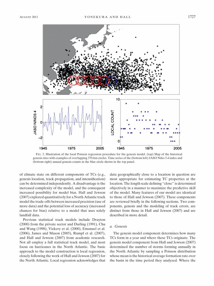
FIG. 2. Illustration of the local Poisson regression procedure for the genesis model. (top) Map of the historical

genesis sites with examples of overlapping 370-km circles. Time series of the (bottom left) JASO Nino-3.4 index and

(bottom right) annual genesis counts in the blue circle shown in the top panel.


TCs originated was determined by random sampling of

an empirical kernel-density function. The Hall and Jewson

(2007) genesis has no climate state sensitivity.

Because ENSO has been shown to influence TC for-

mation in the WNP, it is included in this model. Genesis

is still modeled as a Poisson process, but now the mean

rate is dependent on ENSO state. Poisson regression is

employed, which is the appropriate form of regression

for count data (Sabbatelli and Mann 2007). The de-

pendent variable is the annual formation rate (the mean

Poisson rate) over the full domain, and it is related to the

independent variable, the ENSO index, using a loga-

rithmic link function: lj 5 exp(b0 1 b1 3 ENSOj), where

the b are regression parameters and ENSOj is the value

of the ENSO state index for a specific year j (b1 is

analogous to the slope, and b0 is analogous to the y in-

tercept of linear regression). The regression parameters

are chosen numerically to maximize the likelihood of

the observed annual count time series, given the his-

torical ENSO state index time series. In any particular

year, the Poisson distribution associated with lj is sam-

pled to obtain a simulated TC count for the year.

Next we need to model where in the basin the TCs

form. Local Poisson regression is used to simulate the

local influence of ENSO on genesis. At each point on

a 18 grid the time series of annual TC formation counts

within L 5 370 km (see below for an explanation of the

length scales) of the gridbox center is Poisson regressed

FIG. 3. (a) The x and y displacement values near grid point 348N, 1338E are plotted against each other. The mean

track increment vector is in black as well as the error ellipse defined by the principal axes. (b) As in (a), but now with

the mean x and y increments removed. (c) As in (b), but now rotated to the covariance-ellipse principal axes. (d) As in

(c), but now with the residuals divided by the rms variances along the major (u) and minor (y) covariance-ellipse axes.

In (d) the deviations u and y are now uncorrelated and make up the standardized anomalies to be modeled in-

dependently.


against the time series of ENSO state index. The rates

are divided by the area of the 370-km circle and multi-

plied by the gridbox area to obtain the mean rate on the

grid box. In data-sparse regions regression is omitted,

and the annual mean count is used for the Poisson rate.

(If too few nonzero annual values are available, then the

regression is unstable and is subject to large sampling

error. The threshold value of 5 is somewhat arbitrary,

striking a balance between avoiding local ‘‘hot spots’’

induced by sampling error and avoiding sensitivity to the

threshold of the integrated basinwide rate.) Symboli-

cally, then, in data-rich regions the 18 Poisson rate is

l9j(r) 5 Ag exp[b90(r) 1 b91(r) 3 ENSOj], where r is the

location, Ag is the ratio of the area of the local 18 gridbox

area to the area of the local 370-km circle, and the

primes on l and b indicate that the variables are now

spatially variable.

Figure 2 illustrates the procedure. The IBTrACS

genesis sites are shown on the map, along with several

of the overlapping 370-km data circles. Inset are one

circle’s time series of ENSO values, the independent

variable, and the annual TC formation count in the

circle, the dependent variable. A probability density

function (pdf) is then calculated by dividing the gridded

local Poisson rates by the integrated sum of all local

Poisson rates. Given N total TCs from the basinwide

genesis model, the pdf is sampled N times to obtain the

genesis location of storms in a simulated year with a

given ENSO state.

b. Track propagation

TC propagation occurs by successive simulation of 6-h

track displacements. The model for the 6-h increment is

similar to that of Hall and Jewson (2007). The mean

increment and the variance about the mean are com-

puted locally by a weighted average of nearby historical

increments, with the weighting length scale determined

by out-of-sample minimization of forecast error (the

mean) and maximization of likelihood (the variance).

Also, as in Hall and Jewson (2007), the standardized

errors are modeled as lag-1 autoregression [AR(1)] with

FIG. 4. (a) Historical tracks for 1945–2007 in the IBTrACS archive. (b)–(d) Three independent model realizations

of the historical period. For all panels, a random 20% of the tracks were selected to better see the individual track

shapes.


autocorrelation coefficients computed by distance-

weighted averaging of historical data.

The difference between our analysis and that of Hall

and Jewson (2007) is the procedure to standardize the

errors on which the AR(1) is applied. The AR(1) is

applied independently to the vector components of the

standardized track error, under the assumption that

the components are uncorrelated. The Hall and Jewson

(2007) standardized errors are in a frame of reference

parallel and perpendicular to the local mean track in-

crement, but we have found that this does not always

result in independent error components. Here, the

scatter about the mean increment is allowed to deter-

mine the principal axes of the local error ellipse, and

we standardize the error in this local frame. Using the

data-determined error ellipse frame better ensures

that the components of the 2D standardized errors are

uncorrelated.

The standardizing procedure is illustrated in Fig. 3. In

the scatterplots of Figs. 3a and 3b (with and without

means, respectively) it is clear that the x and y errors

are correlated and, therefore, cannot be modeled in-

dependently. The errors are modeled with a general-

ized two-dimensional normal distribution, in which the

variances in each dimension are allowed to be distinct

and the motions in the two dimensions can covary

(termed a ‘‘bivariate anisotropic correlated normal

distribution’’). The 2D scatter of such a distribution

can be characterized by an error ellipse whose major

axis makes an angle

a 51

2tan21

cxysxsy

s2x 2 s2

y

!

with respect to the x axis (line of constant latitude),

where sx and sy are the rms error variances in the x and

y (longitudinal and latitudinal) directions and cxy is the

x–y error correlation. Rotating the x–y error into the

principal-axes frame of reference (Fig. 3c) results in

transformed errors, u and y, that are independent and

can be modeled as such. In Fig. 3d the errors are divided

by the rms variances in the principal axes to standardize

them. Note that the degree of x–y error correlation

varies spatially and can be as high as 0.8 in some regions,

illustrating the importance of accommodating it.

As in Hall and Jewson (2007) for the North Atlantic,

here for the WNP we have checked for evidence of higher-

order lags and for nonnormality in the errors. Higher

lags are tested by performing multiple-variable regres-

sion of standardized errors against themselves at a

number of lags: i 2 1, i 2 2, i 2 3, and so on. Only lag 1

was found to be significant. Normality was checked with

quantile–quantile analysis. In both the u and y directions

there are deviations from normality beyond 2 standard

deviations. It was a concern that these ‘‘fat tails’’ might

compromise the results, since normality is assumed in

several stages of the analysis—most important, in the

random forcing in the AR(1) model. To test sensitivity,

simulations are performed in which archived historical

errors are randomly sampled rather than using normal

distribution forcing. If fat tails in the errors played a

large role in track propagation, then one would expect

a noticeable difference in simulation behavior between

normal distribution forcing and archived-error sam-

pling. In fact, there was no significant difference in track

behavior according to the diagnostics described below.

c. Lysis

Lysis (the termination of tracks) is identical to that in

Hall and Jewson (2007). The probability P for track lysis

(termination) in a 6-h time step at position r is the ratio

of the weighted sum of all terminal historical track

points to the weighted sum of all track points. Lysis over

ocean and lysis over land are separated using a 0.258

mask to obtain different rates, because the physical pro-

cesses on land and ocean are different.

FIG. 5. Number of TCs crossing longitude lines (1108E–1808

equally spaced left to right) as a function of latitude. Unit in-

crements on x axis are crossings per 58 latitude. (bottom) Westward

crossings; (top) eastward crossings. Dashed lines are historical, and

solid lines are ensemble mean simulation, with shaded gray area

indicating 61 std dev.


d. Optimized averaging scales

In using historical data for each of the model com-

ponents, the weight applied to a datum increases with

geographic proximity to a simulation location in ques-

tion (potential genesis site, current track location, or

potential lysis site). The length scale of the weight de-

termines the balance between the desire to use as many

data as possible (a large scale) and the desire to resolve

geographic structure as well as possible (a small scale).

Hall and Jewson (2007) described year-by-year jack-

knife out-of-sample procedures to determine the length

scales objectively, and we use their procedure here. The

out-of-sample nature of the procedure (use of one data

subset to build the model and use of the remainder

subset to evaluate the model) ensures that the model is

optimized for prediction.

Because we are working here in a different basin with

different data volumes and different geographic distri-

butions of statistical TC properties, the length scales

obtained are not identical to those of Hall and Jewson

(2007). We obtain 370 km for the local Poisson regres-

sion for genesis, 220 km for ocean lysis, 830 km for land

lysis, 220 km for the mean track, and 260 km for the

track variance. As illustrated in Hall and Jewson (2007),

use of scales that are smaller than the optimal scale re-

sults in simulations whose features have unwarranted

fine spatial structure. Use of scales that are larger than

optimal results in excessive smoothing of true geographic

structure. An optimal length scale for the track-error

autocorrelations was not obtained. We used 500 km and

found little sensitivity to varying this value.

e. Simulation

There are four steps to simulate the historical period

(1945–2007):

1) For each of the 63 years, both the basinwide Poisson

rate and a grid of local Poisson rates are calculated

using the historical ENSO state of the respective year.

The associated Poisson distribution for the basinwide

Poisson rate is sampled to give an annual count N for

the basin. The local Poisson rates are used to cal-

culate a normalized pdf that is sampled N times to

give the locations of genesis.

FIG. 6. (a) Historical track density (points per 18 box in the 1945–2007 period), (b) 500-realization ensemble

average track density, and (c) spread of the ensemble, shown by ordering track density values at each grid point and

taking the difference between the 97.5% and 2.5% percentile values. (d) Red regions show where the historical track

point density is above the 97.5% percentile level for that grid point. Blue shows where it is below the 2.5% percentile

level. Green is where the historical values are bounded by the inner 95% of the ensemble.


2) Tracks propagate from the genesis in 6-h time steps. At

each position, the AR(1) model gives the standardized

error ui 5 cuui21 1 s«, where cu is the autocorrelation

coefficient, « is the standard normal random, and

s 5 (1 2 c2u)1/2 is the magnitude of the random term

(Hall and Jewson 2007). A similar expression holds

for the yi, the perpendicular component of the error.

(For the first step cu 5 cy 5 0.) The errors are then

multiplied by the variances in the local principal-

component reference frame and rotated back to the

longitude–latitude frame, and the means are added,

resulting in the next track increment. The simulated

TC position is updated.

3) At each position, lysis is checked by comparing the

local lysis probability P with a uniform random draw

R from 0 to 1. The track is terminated if P . R.

4) The procedure is repeated for all storms produced by

the genesis model for each simulated year, and then

for the desired number of simulations of the 1945–

2007 period.

In the analysis that follows, 500 such simulations were

used. This constitutes the ensemble of simulations of the

1945–2007 period. The model is stochastic, and there-

fore each simulation is distinct.

4. Results

a. Model diagnostics

Figure 4 shows the historical tracks and three re-

alizations of the 63-yr simulations—for example, three

members of the ensemble of simulations. In qualitative

terms, the simulated tracks reproduce the large-scale

features of the historical tracks, propagating westward

in the subtropics and eastward in midlatitudes. We aim

to evaluate the model more quantitatively. The model

performs ‘‘well’’ on a diagnostic to the extent that

the historical value of the diagnostic falls inside some

confidence band of the range of simulated values of

the diagnostic (e.g., the middle 95%). That is, a histor-

ical value should appear to be a typical draw from the

ensemble of simulated values, rather than an outlier.

Where this is not the case, the model is biased with

regard to the diagnostic. Here, the model is evaluated

in this way with respect to three diagnostics: 1) track

crossings of lines of constant longitude, 2) spatial maps

of track density, and 3) landfall rate and its geographic

distribution.

It is important to note that the model is not fit, or

trained, to these diagnostics. The large-scale behavior

of simulated tracks emerges from the point-by-point

stochastic modeling of genesis and the step-by-step

stochastic modeling of 6-hourly track increments.

The model parameters (the averaging length scales)

are chosen objectively to optimize the point and step

processes.

Figure 5 shows eastward and westward track crossings

over lines of constant longitude (counts in 58 latitude

bins) from the historical record and the simulations.

Shown are means across the 500-member simulation

ensemble and the inner 95% range about these means.

This range about the model mean is used as the measure

of significant difference between modeled and historical

track crossings. Where the historical curve falls outside

the spread about the model mean, the model is biased,

FIG. 7. Map of the 47 segments lining the main coast and sig-

nificant other landmasses. Political regions are also marked for

landfall analysis.

FIG. 8. Landfall rates along the eastern Asian coast. The figure

shows the historical (black) and ensemble mean (red), with red

shading for the inner 95% of the simulated landfalls. Units are

counts per 100 kilometers per year.


according to this confidence standard. The behavior of

the mean track is to move westward between 58 and

208N and eastward between 208 and 458N. As can be

seen in the figure, the distribution of east and west track

crossings closely follows that of the historical crossings,

except for a few scattered regions where the historical

curves lie outside the model spread.

Track density (number of 6-h TC points per unit area)

is also used as a diagnostic. Figures 6a and 6b show the

historical and ensemble mean track density, respec-

tively. The overall density distribution is well repro-

duced by the model, but the model overestimates the

maximum in density around the Philippines and un-

derestimates it from Southeast Asia to Japan. Figure 6c

shows the spread of the simulation ensemble—for ex-

ample, the difference between the model’s 2.5% and

97.5% percentile track density value at each grid point.

This range has a maximum where the observed track

density maximum appears. Figure 6d shows a measure

of the significance of the model–observation difference:

regions where the observed track density is above the

97.5% simulation percentile level are red, and regions

where the observed track density is below the 2.5% level

are blue. The regional model disagreements and the

difference in magnitude of the maximum track density

are significant by this standard. We are currently ex-

ploring the reasons for these biases. In other regions the

model shows no coherent bias.

Landfall risk assessment is the ultimate application

of the model, and therefore examining landfall rates

of the simulations is a key diagnostic. The coastline is

divided into segments that are approximately 1000 km

long, covering the Asian mainland; Japan; the Philippines;

Indonesia and Malaysia; and Kamchatka, Russia, as

illustrated in Fig. 7. A landfall occurs on a segment

if a track crosses the segment heading from ocean to

land. The landfalls are accumulated and plotted as

a function of distance along the coastlines in units

of landfalls per year per 100 km of segmented coast-

line. Shown in Fig. 8 are the historical landfall rates,

FIG. 9. Out-of-sample test using landfall data from the 2008–09 period. For each political region, the bars represent

the distribution of landfalls resulting from 1000 model simulations of the out-of-sample period. The asterisk rep-

resents the historical (IBTrACS) values for landfalls in 2008 and 2009.


the model ensemble mean landfall rate, and the mid-

dle 95% range of simulated rates across the ensemble.

There is a high degree of structure in the geographical

distribution of landfall rates, even within regions of

high track density, much of which can be understood in

terms of the relative orientation of coastline segment

and the direction of the mean track. If a coastline seg-

ment is parallel to the local mean track then a landfall is

relatively unlikely, although not impossible, given ran-

dom motions about the mean. If a coastline segment is

perpendicular to the local mean track direction, then

a landfall is relatively likely. Overall, the model cap-

tures the geographical distribution: the local maxima

and minima of the landfall rate are well matched. The

model exhibits low landfall biases in certain regions,

however, consistent with behavior seen in the track den-

sity. Historical landfall counts are above 97.5% of the

model simulations on the coast of China as well as Japan;

that is, the model displays a low landfall bias on these

regions. The model performs well in matching the his-

torical landfalls for the Philippines, and it performs well

on other less-active regions.

Last, 1000 simulations of 2008–09, two out-of-sample

years, are performed using the observed values of the

JASO Nino-3.4 index. The landfall rates are computed

for political regions defined in Fig. 7, and the distributions

are compared with observed landfall rates for 2008–09

(Fig. 9). Results show that the observed rates occur within

the modeled distribution.

b. ENSO dependence

We now turn to the role of ENSO in WNP TC genesis

and, through genesis, its impact on landfall rates. The

results for ENSO’s influence on total genesis and its

geographic distribution confirm those of previous stud-

ies (Chan 1985, 2000; Chia and Ropelewski 2002; Wang

and Chan 2002; Camargo et al. 2007a). The coefficients

from the local Poisson regression are shown in Fig. 10.

Notice that the b1 coefficient that multiplies the ENSO

state variable changes sign from positive in the south-

eastern part of the basin to negative in the northwest.

The implication on genesis rates is further elucidated in

Figs. 11a–c, which show the normalized pdfs produced

using the distribution of annual formation rates from

the Poisson regression for three values of ENSO state

index: 12s, 0, and 22s, where s is 1 standard deviation.

There is a northwestward shift in formation and an in-

crease in the region west of 1408E and south of 308N

from El Nino to La Nina states. The historical genesis

sites at corresponding ENSO states are shown in Figs.

11d–f, and the shifting behavior is evident. This shift is

seen most clearly in Fig. 12, which is a map of the dif-

ference El Nino (12s) minus La Nina (22s).

The dependence of the basinwide annual count on

ENSO (drawn from the Poisson distribution for the

entire basin) is shown in Fig. 13a. The annual count

decreases from 39 to 34 per year with a shift from 22s to

12s in ENSO. Given the indicated 95% range of the

annual counts, this change is barely significant. Figures

13b–d show the annual counts as functions of ENSO

state for subregions of the basin indicated in Fig. 12:

the main development region (MDR; 108–208N, 1108–

1608E), the ‘‘cool’’ region, and the ‘‘warm’’ region. In

the MDR an ENSO change from 22s to 12s decreases

the Poisson rate by five storms per year. In the cool re-

gion, the same 14s ENSO change decreases the

Poisson rate by roughly three storms per year. By

contrast, the warm region has statistically more genesis

activity during El Nino conditions: a 22s to 12s

ENSO shift causes an increase of about three storms

per year. Note that the Poisson regression model is not

linear; genesis sensitivity to a specified change in

ENSO depends on the absolute ENSO value about

which the change occurs.

To determine the significance of these ENSO-genesis

sensitivities, a jackknife test is performed. The counts

are Poisson regressed on ENSO over the basin 10 000

times, in each case randomly dropping 13 (20%) of the

data years used in the regression. In ‘‘delete-d jack-

knife’’ the point is to choose a d . 1 to increase the

number of data subsets across which a statistic can be

computed. For d 5 1 there would be 63 (1945–2007)

subsets of 62 years each, which is not enough to examine

the tails of the distribution—for example, to estimate

FIG. 10. Map of the local beta coefficients (top) b0 and (bottom)

b1 calculated from local Poisson regression of genesis points and

ENSO state.


the 2.5% and 97.5% confidence bounds. For d 5 13

there are 63!/[13!(63 2 13)!] ’ 1012 subsets of 50 years

each. On the other hand, d should not be chosen to be so

large that each subset is too small to allow one to per-

form regression. The value d 5 13 is a compromise.

In Fig. 12, El Nino–minus–La Nina differences are

deemed significantly different than zero at a given lo-

cation if the inner 95% of the differences across the

jackknife set have the same sign. Locations where this is

true are indicated in Fig. 12 with plus symbols. The re-

gions of largest ENSO sensitivity are all significant by

this measure. The same jackknife test is used to put

confidence bounds (middle 95%) on formation rates

as a function of ENSO (Fig. 13). These bounds suggest

that ENSO sensitivity is significant on a regional basis.

The basinwide decline in formation rates with increasing

ENSO state (Fig. 13a) is fractionally smaller than the

regional changes because of cancellation due to oppos-

ing sensitivities in the warm and cool regions. To test the

significance of basinwide sensitivity, the distribution of

b1 coefficients (the coefficient multiplying the ENSO

value) is examined across the set of jackknife basinwide

FIG. 11. (left) Maps of normalized probability distribution function from local Poisson rates, given the JASO Nino-

3.4 index values of (a) 2s, (b) 22s, and (c) 0. (right) The corresponding IBTrACS genesis sites for years with JASO

Nino-3.4 index values of (d) greater than s, (e) less than 2s, and (f) less than s but greater than 2s. The red point

marks the mean genesis location.


regressions. The 2.5% and 97.5% percentile values of

these b1 are roughly 20.06 and 20.01, respectively, in-

dicating that the basinwide formation decline with

ENSO is significant. Thus, although we agree with the

findings of Camargo and Sobel (2005) and Wang and

Chan (2002) that basinwide formation sensitivity to

ENSO is fractionally miniscule in comparison with re-

gional sensitivity, we find the small sensitivity to be

significant.

Both the change in basinwide rates and the shift in

distribution with ENSO have consequences for landfall

rates. During a La Nina event more TCs form in the

basin and they form closer to the Asian coast. The im-

pact of ENSO on landfall rates is shown in Fig. 14. Fifty

model simulations of 1945–2007 are performed, each

with a different fixed value of ENSO. The ensemble

mean landfall profile is computed for each ENSO value.

For most regions La Nina results in higher landfall than

does El Nino. This is illustrated in Table 1, where the

landfall rates of several political regions defined in Fig. 7

are shown for different ENSO states. For example, the

central Pacific (CP) Asian coastline has a landfall rate

increase of 40% for an ENSO change from 22s to 12s.

For the same change, the Philippines show a 9.5%

landfall rate increase.

To highlight better the regional effects of ENSO state

on landfall rates, Fig. 15 shows the fractional change

in landfall rates for regions defined in Fig. 7. All re-

gions show a decrease in fractional change with in-

creasing value of ENSO state index. The change is

most drastic from a strong La Nina event to a neutral

state for Indonesia/Malaysia, the northeastern main-

land coast, and Japan. This result does not agree with

previous work (Wu et al. 2004; Saunders et al. 2000;

Elsner and Liu 2003) that finds increased landfalls on

Japan, the Korean peninsula, and northern China during

El Nino events.

5. Discussion

We have developed a new statistical model for WNP

typhoon tracks and genesis on the basis of IBTrACS

data. The primary application is estimating Asian ty-

phoon landfall rates on a regional scale and their sen-

sitivity to ENSO. Model parameters (length scale in the

local regression) are determined by an out-of-sample

procedure to maximize the model’s ability to forecast.

The model captures well the overall features of WNP

typhoon genesis and propagation, realistically reproduc-

ing both mean structure and pseudorandom variation

FIG. 12. Pdf difference of using ENSO state anomaly of 2 and 22. The crosses mark the

regions where the sign of the difference remains the same for the inner 95% of the bootstrap

reconstructions of the genesis model that dropped out a random 20% of the data. The white box

defines the MDR, the red box denotes the warm region, and the blue box denotes the cool

region.


about the mean. The geographic distribution of landfall

rates is reproduced well in both historically active regions

and in less-active regions. The realistic behavior in less-

active regions (e.g., Indonesia and Malaysia) is encour-

aging: a track model should be most advantageous over

a model that is based solely on historical landfalls in re-

gions where landfalls are rare.

The analysis reveals some model biases whose sources

remain to be isolated and corrected. The discrepancy

in track point density indicates that the model may be

moving the storms too slowly to reach the coastal areas.

This gives storms more chance to suffer lysis before mak-

ing landfall, resulting in the low landfall biases seen for

certain regions. The model also places roughly 58 too far

south the latitude of maximum eastward storm propa-

gation in midlatitudes (Fig. 5a). Many of the historic storms

in this region have undergone extratropical transition,

which may affect their propagation but has not been

explicitly considered here.

The genesis model has been constructed to be sensi-

tive to ENSO. Regions of peak formation shift south-

eastward during El Nino and northwestward during La

Nina, in agreement with results of previous studies. The

combined effects of a marginally significant increase in

overall storms and formation closer to land result in

more landfalls during La Nina. Important ENSO effects

FIG. 13. Annual formation counts for different phases of ENSO for the (a) entire domain, (b) MDR, (c) cool

region, and (d) warm region as defined in Fig. 12. Dashed lines indicate the inner 95% range from the jackknife

method, and the solid line is the mean of 1000 jackknife versions of the genesis model.

FIG. 14. Landfall rates from 50-realization model runs of the

historical period given a stationary value of JASO Nino-3.4 anom-

aly. Positive anomalies are El Nino years, and negative anomalies

are La Nina years.


remain to be included in the model, however, which may

modify these results. Other studies (Wang and Chan

2002; Elsner and Liu 2003; Camargo et al. 2007b) argue

that TC track shapes are sensitive to ENSO. Some of this

effect is included in the sensitivity of the genesis distri-

bution, because TCs forming in different regions will

follow different trajectories according to the model.

There may be additional influence that is currently not

included that could be introduced by explicitly adding

ENSO sensitivity to the track propagation component of

the model. This may help to account for the differences

in landfall sensitivity to ENSO found in this study when

compared with previous studies. One crucial aspect is

that an intensity model has not yet been implemented,

and all landfalls are treated equally. TCs in El Nino

years form farther from the coast and, therefore, have

more time to intensify before making landfall (Wang

and Chan 2002; Chan and Liu 2004; Chan 2005, 2006;

Camargo and Sobel 2005; Camargo et al. 2007a). Thus,

even though La Nina years have more overall landfalls,

El Nino years are more likely to produce the intense

landfalls that dominate risk-assessment considerations.

This idea will be explored further once an intensity

model is implemented.

Acknowledgments. This work was supported in part

by a grant from the NASA Applied Sciences pro-

gram. The authors are grateful to Suzana Camargo

and Anthony Del Genio for helpful comments on this

work.

REFERENCES

Barnston, A. G., M. Chelliah, and S. B. Goldenberg, 1997: Docu-

mentation of a highly ENSO-related SST region in the equa-

torial Pacific. Atmos.–Ocean, 35, 367–383.

Camargo, S. J., and A. H. Sobel, 2005: Western North Pacific

tropical cyclone intensity and ENSO. J. Climate, 18, 2996–

3006.

——, K. A. Emanuel, and A. H. Sobel, 2007a: Use of a genesis

potential index to diagnose ENSO effects on tropical cyclone

genesis. J. Climate, 20, 4819–4834.

——, A. W. Robertson, S. J. Gaffney, P. Smyth, and M. Ghil,

2007b: Cluster analysis of typhoon tracks. Part II: Large-scale

circulation and ENSO. J. Climate, 20, 3654–3676.

Chan, J. C. L., 1985: Tropical cyclone activity in the northwest

Pacific in relation to the El Nino/Southern Oscillation phe-

nomenon. Mon. Wea. Rev., 113, 599–606.

——, 2000: Tropical cyclone activity over the western North Pacific

associated with El Nino and La Nina events. J. Climate, 13,

2960–2972.

——, 2005: Interannual and interdecadal variations of tropical

cyclone activity over the western North Pacific. Meteor. At-

mos. Phys., 89, 143–152.

——, 2006: Comment on ‘‘Changes in tropical cyclone number,

duration, and intensity in a warming environment.’’ Science,

311, 1713.

——, and J. Shi, 2000: Frequency of typhoon landfall over

Guangdong Province of China during the period 1470–1931.

Int. J. Climatol., 20, 183–190.

——, and K. S. Liu, 2004: Global warming and western North

Pacific typhoon activity from an observational perspective.

J. Climate, 17, 4590–4602.

Chia, H.-H., and C. F. Ropelewski, 2002: The interannual vari-

ability in the genesis location of tropical cyclones and the

northwest Pacific. J. Climate, 15, 2934–2944.

Chu, P., and J. Wang, 1998: Modeling return periods of tropical

cyclone intensities in the vicinity of Hawaii. J. Appl. Meteor.,

39, 951–960.

Darling, R., 1991: Estimating probabilities of hurricane wind speeds

using a large-scale empirical model. J. Climate, 4, 1035–1046.

TABLE 1. Landfall rates, in units of landfalls per year per 100 km for specific political regions, given different Nino-3.4 JASO values.

The bottom row shows the change from a 12 to a 22 phase of ENSO. The last column gives the genesis rates, in TC per year, for each

ENSO state.

ENSO state SE Asia CP Asia NE Asia Japan Philippines All Genesis rates

2 0.06 0.08 0.01 0.04 0.12 0.05 34.04

0 0.07 0.10 0.02 0.05 0.14 0.06 36.53

22 0.07 0.11 0.02 0.06 0.13 0.07 39.21

% change* 17.82 40.80 47.58 40.82 9.51 26.26 15.19

* For rate r, % change is [r(ENSO 5 22) 2 r(ENSO 5 12)]/r(ENSO 5 12).

FIG. 15. Fractional change in landfall for political regions given

a stationary value of ENSO anomaly.


Dong, K., 1988: El Nino and tropical cyclone frequency in the

Australian region and the northwest Pacific. Aust. Meteor.

Mag., 36, 219–255.

Drayton, M., 2000: A stochastic ‘‘basin-wide’’ model of Atlantic

hurricanes. Proc. 24th Conf. on Hurricanes and Tropical Me-

teorology, Ft. Lauderdale, FL, Amer. Meteor. Soc., 17A.3.

Elsner, J. B., and K. B. Liu, 2003: Examining the ENSO–typhoon

hypothesis. Climate Res., 25, 43–54.

——, R. J. Murnane, and T. H. Jagger, 2006: Forecasting U.S.

hurricanes 6 months in advance. Geophys. Res. Lett., 33,

L10704, doi:10.1029/2006GL025693.

Emanuel, K., S. Ravela, E. Vivant, and C. Risi, 2006: A statistical

deterministic approach of hurricane risk assessment. Bull.

Amer. Meteor. Soc., 87, 299–314.

Fudeyasu, H., S. Iizuka, and T. Matsuura, 2006: Impact of ENSO

on landfall characteristics of tropical cyclones over the west-

ern North Pacific during the summer monsoon season. Geo-

phys. Res. Lett., 33, L21815, doi:10.1029/2006GL027449.

Hall, T. M., and S. Jewson, 2007: Statistical modeling of North

Atlantic tropical cyclone tracks. Tellus, 59A, 486–498.

Harr, P. A., and R. L. Elsberry, 1991: Tropical cyclone track

characteristics as a function of large-scale circulation anoma-

lies. Mon. Wea. Rev., 119, 1448–1468.

James, M. K., and L. B. Mason, 2005: Synthetic tropical cyclone

database. J. Waterw. Port Ocean Eng., 131 (4), 181–192.

Knapp, K. R., M. C. Kruk, D. H. Levinson, H. J. Diamond, and

C. J. Neumann, 2010: The International Best Track Ar-

chive for Climate Stewardship (IBTrACS): Unifying trop-

ical cyclone best track data. Bull. Amer. Meteor. Soc., 91,363–376.

Rumpf, J., H. Weindl, P. Hoppe, E. Rauch, and V. Schmidt, 2007:

Stochastic modeling of tropical cyclone tracks. Math. Methods

Oper. Res., 66, 475–490.

Sabbatelli, T. A., and M. E. Mann, 2007: The influence of climate

state variables on Atlantic tropical cyclone occurrence rates.

J. Geophys. Res., 112, D17114, doi:10.1029/2007JD008385.

Saunders, M. A., R. E. Chandler, C. J. Merchant, and F. P. Roberts,

2000: Atlantic hurricanes and NW Pacific typhoons: ENSO

spatial impacts on occurrence and landfall. Geophys. Res.

Lett., 27, 1147–1150.

Vickery, P. J., P. F. Skerlj, and L. A. Twisdale, 2000: Simulation

of hurricane risk in the U.S. using an empirical track model.

J. Struct. Eng., 126, 1222–1237.

Wang, B., and J. C. L. Chan, 2002: How strong ENSO events affect

tropical storm activity over the western North Pacific. J. Cli-

mate, 15, 1643–1658.

Wu, M. C., W. L. Chang, and W. M. Leung, 2004: Impacts of

El Nino–Southern Oscillation events on tropical cyclone

landfalling activity in the western North Pacific. J. Climate, 17,

1419–1428.


A Statistical Model of Tropical Cyclone Tracks in the … · · 2013-04-10A Statistical Model of...

Documents

Transcript of A Statistical Model of Tropical Cyclone Tracks in the … · · 2013-04-10A Statistical Model of...