THE RAMANUJAN JOURNAL, 4, 251–265, 2000c© 2000 Kluwer Academic Publishers. Manufactured in The Netherlands.

A q-Analogue of Weber-Schafheitlin Integralof Bessel Functions∗

MIZAN RAHMAN mrahman@math.carleton.caSchool of Mathematics and Statistics, Carleton University, Ottawa, Ont. K1S 5B6

Received May 10, 1999; Accepted May 11, 1999

Abstract. In an attempt to find aq-analogue of Weber and Schafheitlin’s integral∫∞

0 x−ρ Jµ(ax)Jν(bx) dx

which is discontinuous on the diagonala = b the integral∫∞

0 x−ρ J(2)ν (a(1− q)x;q)J(1)µ (b(1− q)x;q) dx is

evaluated whereJ(1)µ (x;q) and J(2)µ (x;q) are two of Jackson’s threeq-Bessel functions. It is found that thequestion of discontinuity becomes irrelevant in this case. Evaluations of this integral are also made in someinteresting special cases. A biorthogonality formula is found as well as a Neumann series expansion forxρ interms ofJ(2)ν+1+2n((1− q)x;q). Finally, aq-Lommel function is introduced.

Key words: Weber-Schafheitlin integral,q-Bessel functions, Ramanujan integral, basic hypergeometric series,q-integrals,q-Lommel function,q-Neumann series

2000 Mathematics Subject Classification: Primary–33D15; Secondary–33D45

1. Introduction

One of the most fascinating formulas in the theory of Bessel functions is the followingintegral of Weber and Schafheitlin [21, §13.4(2)]:∫ ∞

0Jµ(at)Jν(bt)t−ρ dt

= 2−ρaµbρ−µ−1 0( 1−ρ+µ+ν

2

)0(µ+ 1)0

( 1+ρ+ν−µ2

) 2F1

[ 1−ρ+µ+ν2 ,

1−ρ+µ−ν2

µ+ 1; a2

b2

], (1.1)

provided 0< a < b and−1< Reρ < Re(µ+ ν + 1). For 0< b < a the correspondingformula is obtained by interchangingµ andν as well asa andb, so there is a discontinuityon the diagonala = b where the integral has the value∫ ∞

0Jµ(at)Jν(at)t−ρ dt

= 0(ρ)0( 1−ρ+µ+ν

2

)(a/2)ρ−1

20( 1+ρ+µ−ν

2

)0( 1+ρ+ν−µ

2

)0( 1+ρ+µ+ν

2

) . (1.2)

∗This work was supported by NSERC grant #A6197.

252 RAHMAN

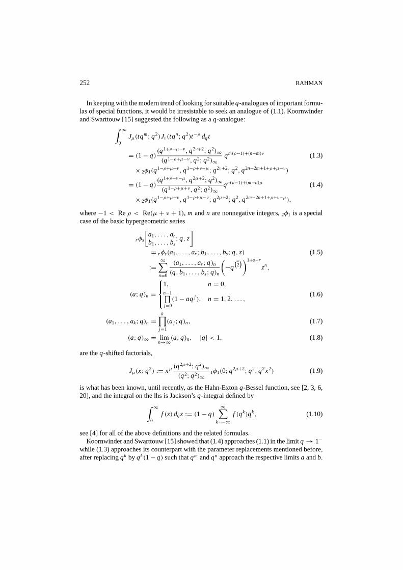
In keeping with the modern trend of looking for suitableq-analogues of important formu-las of special functions, it would be irresistable to seek an analogue of (1.1). Koornwinderand Swarttouw [15] suggested the following as aq-analogue:∫ ∞

0Jµ(tq

m;q2)Jν(tqn;q2)t−ρ dqt

= (1− q)(q1+ρ+µ−ν,q2ν+2;q2)∞(q1−ρ+µ−ν,q2;q2)∞

qm(ρ−1)+(n−m)ν (1.3)

× 2φ1(q1−ρ+µ+ν,q1−ρ+ν−µ;q2ν+2;q2,q2n−2m+1+ρ+µ−ν)

= (1− q)(q1+ρ+ν−µ,q2µ+2;q2)∞(q1−ρ+µ+ν,q2;q2)∞

qn(ρ−1)+(m−n)µ (1.4)

× 2φ1(q1−ρ+µ+ν,q1−ρ+µ−ν;q2µ+2;q2,q2m−2n+1+ρ+ν−µ),

where−1 < Reρ < Re(µ + ν + 1), m andn are nonnegative integers,2φ1 is a specialcase of the basic hypergeometric series

rφs

[a1, . . . ,ar

b1, . . . ,bs;q, z

]= rφs(a1, . . . ,ar ; b1, . . . ,bs;q, z) (1.5)

:=∞∑

n=0

(a1, . . . ,ar ;q)n(q, b1, . . . ,bs;q)n

(−q(n

2))1+s−r

zn,

(a;q)n =

1, n = 0,n−1∏j=0(1− aqj ), n = 1, 2, . . . ,

(1.6)

(a1, . . . ,ak;q)n =k∏

j=1

(aj ;q)n, (1.7)

(a;q)∞ = limn→∞(a;q)n, |q| < 1, (1.8)

are theq-shifted factorials,

Jµ(x;q2) := xµ(q2µ+2;q2)∞(q2;q2)∞

1φ1(0;q2µ+2;q2,q2x2) (1.9)

is what has been known, until recently, as the Hahn-Extonq-Bessel function, see [2, 3, 6,20], and the integral on the lhs is Jackson’sq-integral defined by∫ ∞

0f (z) dqz := (1− q)

∞∑k=−∞

f (qk)qk, (1.10)

see [4] for all of the above definitions and the related formulas.Koornwinder and Swarttouw [15] showed that (1.4) approaches (1.1) in the limitq→ 1−

while (1.3) approaches its counterpart with the parameter replacements mentioned before,after replacingqk by qk(1− q) such thatqm andqn approach the respective limitsa andb.

A q-ANALOGUE 253

For thisq-analogue, however, the continuity question does not arise because of the discretedomains, but the expressions on the right sides of (1.3) and (1.4) are equal which is, ofcourse, not true in the limitq→ 1−. The equality of these expressions is not immediatelyobvious but can be proved by using the 3-term transformation formula [4, III.32] for which,however, it is essential that|m− n| is a nonnegative integer.

The purpose of this paper is to look for anotherq-analogue of (1.1) that is not restricted todiscrete domains. However, in a problem dealing with aq-Bessel function the first questionto settle is which analogue we are talking about. Jackson [12] is known to be the first oneto introduce two analogues of Bessel functions:

J(1)ν (x;q) = (qν+1;q)∞(q;q)∞

∞∑n=0

(−1)n(x/2)ν+2n

(q,qν+1;q)n , (1.11)

0< q < 1, |x| < 2, and

J(2)ν (x;q) = (qν+1;q)∞(q;q)∞

∞∑n=0

(−1)n(x/2)ν+2n

(q,qν+1;q)n qn(ν+n). (1.12)

Hahn [5] showed that

J(2)ν (x;q) = (−x2/4;q)∞ J(1)ν (x;q), |x| < 2. (1.13)

Both these analogues have been studied extensively by Mourad Ismail in [7] and [8]. In arecent article Ismail [9] pointed out that Jackson had even a third analogue:

J(3)ν (x;q) = xν(qν+1;q)∞2ν(q;q)∞ 1φ1(0;qν+1;q,qx2/4), (1.14)

which is essentially the same as (1.9) in baseq instead ofq2. Since Jackson’s work precedesthat of Hahn by about 50 years and of Exton by 74, Ismail suggests that the function in (1.14)and (1.9) be called Jackson’sJ(3)ν q-Bessel function. The superscripted notation for all threeq-Bessel functions of Jackson is due to Ismail. All of them satisfy the limit property:

limq→1−

J(i )ν (x(1− q);q) = Jν(x), i = 1, 2, 3. (1.15)

More recently, first Koelink [14] and then independently Ismail, Masson and Suslov,[10, 11], introduced anotherq-analogue which, following the notation and normalizationof the latter authors, is

Jν(z, r ) :=( r

2

)ν (qν+1,−r 2/4;q)∞(q;q)∞ 2φ1

[zq

ν+12 ,q

ν+12/

zqν+1 ;q,−r 2/4

], (1.16)

where|z| = 1. It can be shown that

limq→1−

Jν(e2i θ , r (1− q)) = Jν(2r sinθ), 0≤ θ < π. (1.17)

254 RAHMAN

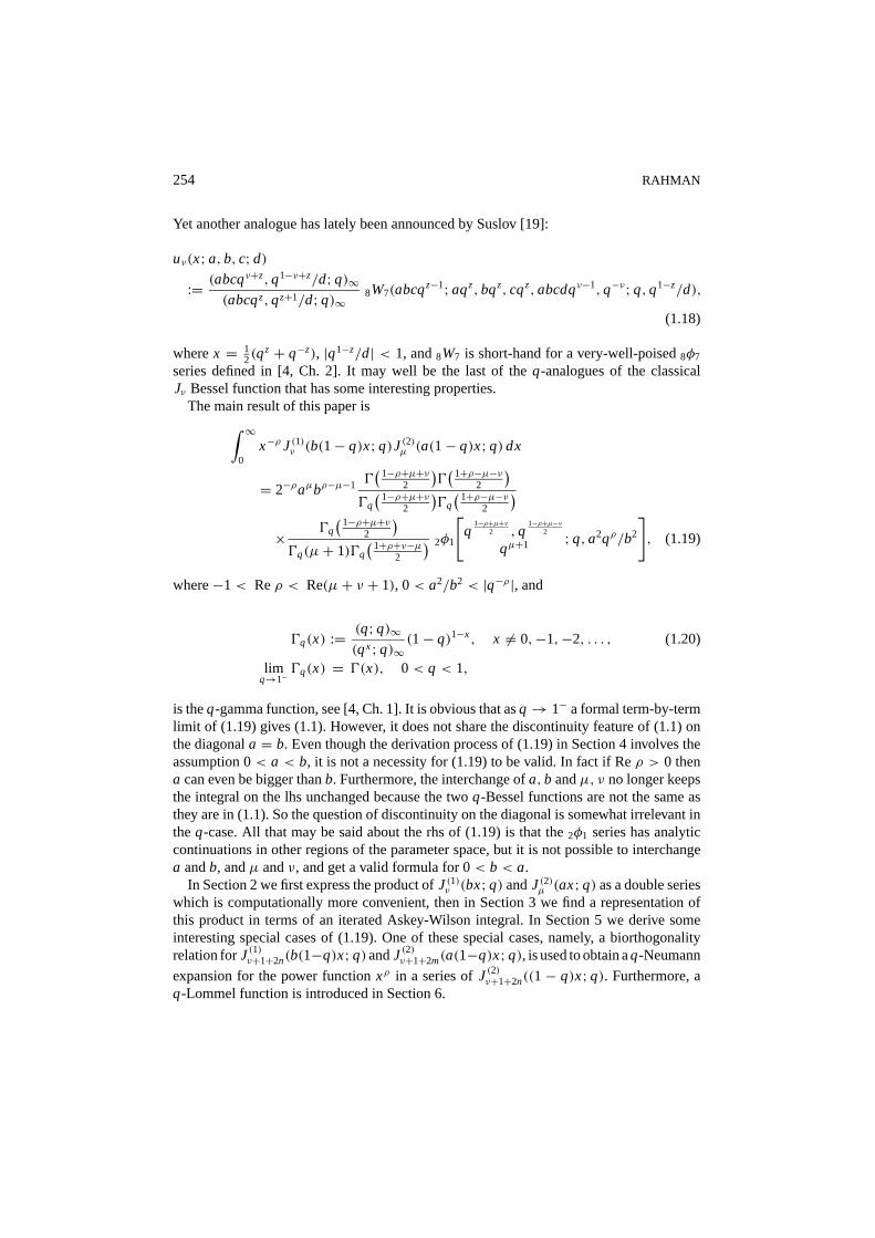
Yet another analogue has lately been announced by Suslov [19]:

uν(x;a, b, c; d):= (abcqν+z,q1−ν+z/d;q)∞

(abcqz,qz+1/d;q)∞ 8W7(abcqz−1;aqz, bqz, cqz,abcdqν−1,q−ν;q,q1−z/d),

(1.18)

wherex = 12(q

z + q−z), |q1−z/d| < 1, and8W7 is short-hand for a very-well-poised8φ7

series defined in [4, Ch. 2]. It may well be the last of theq-analogues of the classicalJν Bessel function that has some interesting properties.

The main result of this paper is∫ ∞0

x−ρ J(1)ν (b(1− q)x;q)J(2)µ (a(1− q)x;q) dx

= 2−ρaµbρ−µ−1 0( 1−ρ+µ+ν

2

)0( 1+ρ−µ−ν

2

)0q( 1−ρ+µ+ν

2

)0q( 1+ρ−µ−ν

2

)× 0q

( 1−ρ+µ+ν2

)0q(µ+ 1)0q

( 1+ρ+ν−µ2

) 2φ1

[q

1−ρ+µ+ν2 ,q

1−ρ+µ−ν2

qµ+1 ;q,a2qρ/b2

], (1.19)

where−1< Reρ < Re(µ+ ν + 1), 0< a2/b2 < |q−ρ |, and

0q(x) := (q;q)∞(qx;q)∞ (1− q)1−x, x 6= 0,−1,−2, . . . , (1.20)

limq→1−

0q(x) = 0(x), 0< q < 1,

is theq-gamma function, see [4, Ch. 1]. It is obvious that asq→ 1− a formal term-by-termlimit of (1.19) gives (1.1). However, it does not share the discontinuity feature of (1.1) onthe diagonala = b. Even though the derivation process of (1.19) in Section 4 involves theassumption 0< a < b, it is not a necessity for (1.19) to be valid. In fact if Reρ > 0 thena can even be bigger thanb. Furthermore, the interchange ofa, b andµ, ν no longer keepsthe integral on the lhs unchanged because the twoq-Bessel functions are not the same asthey are in (1.1). So the question of discontinuity on the diagonal is somewhat irrelevant intheq-case. All that may be said about the rhs of (1.19) is that the2φ1 series has analyticcontinuations in other regions of the parameter space, but it is not possible to interchangea andb, andµ andν, and get a valid formula for 0< b < a.

In Section 2 we first express the product ofJ(1)ν (bx;q) andJ(2)µ (ax;q) as a double serieswhich is computationally more convenient, then in Section 3 we find a representation ofthis product in terms of an iterated Askey-Wilson integral. In Section 5 we derive someinteresting special cases of (1.19). One of these special cases, namely, a biorthogonalityrelation forJ(1)ν+1+2n(b(1−q)x;q)andJ(2)ν+1+2m(a(1−q)x;q), is used to obtain aq-Neumann

expansion for the power functionxρ in a series ofJ(2)ν+1+2n((1− q)x;q). Furthermore, aq-Lommel function is introduced in Section 6.

A q-ANALOGUE 255

2. A product formula

Let us assume thata, b, x are real and 0< a ≤ b, x ≥ 0. Then, for Re(µ, ν) > −1,

J(1)ν (bx;q)J(2)µ (ax;q)

= (qν+1,qµ+1;q)∞(q,q;q)∞

(ax

2

)µ(bx

2

)ν∞∑

n=0

(−b2x2/4)n

(q,qν+1;q)n 2φ1

[q−ν−n,q−n

qµ+1 ;q, a2

b2qµ+ν+1+2n

], (2.1)

by (1.10) and (1.11). Ifa = b then the2φ1 series above can be summed by [4, (II.7)], so thedouble series on the rhs of (2.1) becomes a single4φ3 series, see [17, (1.20)]. Whena 6= bbut ν = µ the2φ1 series is a well-poised series which can be transformed into a balanced4φ3 series that eventually leads to a nice integral representation of the product on the lhsof (2.1). See [17] for details. However, whena 6= b andν 6= µ the 2φ1 series has noneof these properties, so we need to use other transformation formulas in order to producea usable integral representation. By using [4, (1.4.5)] and [4, (1.5.4)] in this order, wefind that

2φ1

[q−ν−n,q−n

qµ+1 ;q, c2qν+µ+1+2n

]= (qµ+1+n, c2qµ+ν+1+n;q)∞

(qµ+1, c2qµ+ν+1+2n;q)∞ 2φ1

[c2,q−n

c2qµ+ν+1+n;q,qµ+1+n

]= (c2qµ+ν+1+n, c2qµ+1+n;q)∞

(qµ+1, c2qµ+ν+1+2n;q)∞ 2φ2

[c2, c2qµ+ν+1+2n

c2qµ+1+n, c2qµ+ν+1+n;q,qµ+1

]= (c2qµ+1;q)∞

(qµ+1;q)∞∞∑

m=0

(c2;q)m(c2qµ+ν+1;q)2n+m

(q;q)m(c2qµ+1, c2qµ+ν+1;q)n+m(−1)mq

(m2)+(µ+1)m

. (2.2)

Use of the identify(a;q)2n = (a1/2,−a1/2, (aq)1/2,−(aq)1/2;q)n then leads to the productformula

J(1)ν (bx;q)J(2)µ (ax;q)

=(qν+1, a2

b2 qµ+1;q)∞(q,q;q)∞

(ax

2

)µ(bx

2

)ν ∞∑m=0

(a2/b2;q)m(−1)mq(m

2)+(µ+1)m

(q,a2qµ+1/b2;q)m

× 4φ3

[abq

µ+ν+m+12 ,− a

bqµ+ν+m+1

2 , abq

µ+ν+m+22 ,− a

bqµ+ν+m+2

2

qν+1, a2

b2 qµ+1+m, a2

b2 qµ+ν+1+m;q,−b2x2/4

]. (2.3)

It may seem a bit strange that of all the other transformation formulas available for theterminating2φ1 series on the lhs of (2.2), see [4, Appendix III], we have chosen to use thetwo that transform it to a much more complicated-looking infinite series. Obviously we

256 RAHMAN

have tried almost every other combination, but each one of them seems to lead to somedivergence problems when one tries to use this product formula in calculating aq-analogueof (1.1). This is the only one that works.

3. An integral representation

Our next step is to find an integral representation of the rhs of (2.3), specifically the4φ3

series. Using the notation of [4, Ch. 6]

h(x;a) :=∞∏

n=0

(1− 2axqn + a2q2n) = (aei θ ,ae−i θ ;q)∞, x = cosθ, (3.1)

h(x;a1, . . . ,am) :=∞∏

k=1

h(x;ak), (3.2)

w(x;a, b, c, d) := (1− x2)−1/2 h(x; 1,−1,q1/2,−q1/2)

h(x;a, b, c, d) , (3.3)

and the well-known Askey-Wilson integral [4, (6.1.1)], we find that

4φ3

[cq

µ+ν+m+12 ,−cq

µ+ν+m+12 , cq

µ+ν+m+22 ,−cq

µ+ν+m+22

qν+1, c2qµ+1+m, c2qµ+ν+1+m ;q,−t2

]

= (q, c2qµ+ν+m;q)∞2π(cq

µ+ν+m2 , cq

µ+ν+m+22 ;q)∞

×∫ 1

−1w(y; c1/2q

µ+ν+m+24 ,−c1/2q

µ+ν+m+24 , c1/2q

µ+ν+m4 ,−c1/2q

µ+ν+m4)

× 3φ2

[cq

µ+ν+m+22 , c1/2q

µ+ν+m+24 eiφ, c1/2q

µ+ν+m+24 e−iφ

qν+1, c2qµ+1+m ;q,−t2

]dy, (3.4)

y = cosφ. The integral on the rhs converges because of our assumption that 0< a < b,Re(µ, ν) > −1. We shall apply [4, (6.1.1)] once again, on the above3φ2 series, but nowwe need to make an interim assumption that Re(µ − ν) ≥ 0. Then the3φ2 series can bewritten as (

q, cqµ+ν+m+2

2 , cqµ−ν+m

2 ;q)∞h(y; c1/2q

µ+ν+m+24 , c3/2q

3µ−ν+3m+24

)2π(c2qµ+1+m;q)∞

×∫ 1

−1w(z;q ν+1

2 , cqµ+1+m

2 , c1/2qµ−ν+m

4 eiφ, c1/2qµ−ν+m

4 e−iφ)

× 2φ1

[qν+1

2 eiψ,qν+1

2 e−iψ

qν+1 ;q,−t2

]dz, (3.5)

A q-ANALOGUE 257

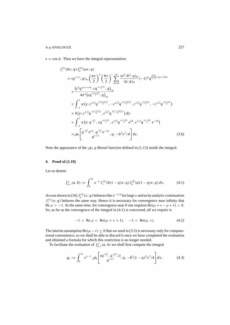
z= cosψ . Thus we have the integral representation:

J(1)ν (bx;q)J(2)µ (ax;q)

= (qν+1;q)∞(

ax

2

)µ(bx

2

)ν ∞∑m=0

(a2/b2;q)m(q;q)m (−1)mq

(m2)+(µ+1)m

×(c2qµ+ν+m, cq

µ−ν+m2 ;q)∞

4π2(cq

µ+ν+m2 ;q)∞

×∫ 1

−1w(y; c1/2q

µ+ν+m+24 ,−c1/2q

µ+ν+m+24 , c1/2q

µ+ν+m4 ,−c1/2q

µ+ν+m4)

× h(y; c1/2q

µ+ν+m+24 , c3/2q

3µ−ν+3m+24

)dy

×∫ 1

−1w(z;q ν+1

2 , cqµ+1+m

2 , c1/2qµ−ν+m

4 eiφ, c1/2qµ−ν+m

4 e−iφ)

×2φ1

[qν+1

2 eiψ,qν+1

2 e−iψ

qν+1 ;q,−b2x2/4

]dz. (3.6)

Note the appearance of the2φ1 q-Bessel function defined in (1.13) inside the integral.

4. Proof of (1.19)

Let us denote

f ρµ,ν(a, b) :=∫ ∞

0x−ρ J(1)ν (b(1− q)x;q)J(2)µ (a(1− q)x;q) dx. (4.1)

As was shown in [16]J(2)µ (x;q)behaves likex−1/2 for largex and so by analytic continuationJ(1)ν (x;q) behaves the same way. Hence it is necessary for convergence near infinity thatReρ > −1. At the same time, for convergence near 0 one requires Re(µ+ ν−ρ+1) > 0.So, as far as the convergence of the integral in (4.1) is concerned, all we require is

−1< Reρ < Re(µ+ ν + 1), −1< Re(µ, ν). (4.2)

The interim assumption Re(µ−ν) ≥ 0 that we used in (3.5) is necessary only for computa-tional convenience, so we shall be able to discard it once we have completed the evaluationand obtained a formula for which this restriction is no longer needed.

To facilitate the evaluation off ρµ,ν(a, b) we shall first compute the integral

gλ :=∫ ∞

0xλ−1

2φ1

[zq

ν+12 ,q

ν+12 /z

qν+1 ;q,−b2(1− q)2x2/4

]dx, (4.3)

258 RAHMAN

|z| = 1, Reλ > 0. Obviously we cannot do the term-by-term integration, so we first usethe transformation formula [4, (III.1)] to get

gλ =(qν+1

2/

z;q)∞(qν+1;q)∞

∞∑r=0

(zq

ν+12 ;q)

r

(q;q)r(qν+1

2/

z)r

×∫ ∞

0xλ−1

(− b2(1−q)2z qr+ ν+12

4 x2;q)∞(− b2(1−q)2

4 qr x2;q)∞ dx. (4.4)

By an obvious transformation the integral on the rhs of (4.4) is

1

2

(2q−r/2

b(1− q)

)λ ∫ ∞0

tλ2−1

(−zqν+1

2 t;q)∞(−t;q)∞ dt

= 1

2

(2q−r/2

b(1− q)

)λ 0( λ2)0(1− λ2

)0q(λ2

)0q(1− λ

2

) (q, zq

ν+12 ;q)∞(

qλ/2, zqν−λ+1

2 ;q)∞ (1− q), (4.5)

by Ramanujan’s [18] well-known integral formula. Thus,

gλ =(

2

1− q

)λ−1

b−λ0(λ2

)0(1− λ

2

)0q(λ2

)0q(1− λ

2

) (q;q)∞h(z;q ν+1

2)(

qν+1,qλ/2, zqν−λ+1

2 ;q)∞×∞∑

r=0

(zq

ν+12 ;q)

r

(q;q)r(qν−λ+1

2/

z)r

=(

2

1− q

)λ−1

b−λ0(λ2

)0(1− λ

2

)0q(λ2

)0q(1− λ

2

) (q,qν+1− λ2 ;q)∞(

qν+1,qλ/2;q)∞h(z;q ν+1

2)

h(z;q ν−λ+1

2) , (4.6)

by use of theq-binomial formula [4, (II.3)]. For application in (4.1) we need to useλ =µ+ ν + 1− ρ, so

gµ+ν+1−ρ =(

2

1− q

)µ+ν−ρbρ−µ−ν−1 0

(µ+ν+1−ρ

2

)0( 1+ρ−µ−ν

2

)0q(µ+ν+1−ρ

2

)0q( 1+ρ−µ−ν

2

)×(q,q

ν−µ+1+ρ2 ;q)∞(

qµ+ν+1−ρ

2 ;q)∞h(z;q ν+1

2)

h(z;q ρ−µ

2) . (4.7)

At this point we need to make another interim assumption: Re(ρ − µ) > 0. From (3.6),

A q-ANALOGUE 259

(4.1) and (4.7) we obtain

f ρµ,ν(a, b)

=(

1− q

2

)ρ(a

b

)µbρ−1 0

(µ+ν+1−ρ

2

)0( 1+ρ−µ−ν

2

)0q(µ+ν+1−ρ

2

)0q( 1+ρ−µ−ν

2

) (q,q ν−µ+1+ρ2 ;q)∞(

qµ+ν+1−ρ

2 ;q)∞×∞∑

m=0

(a2/b2;q)m(q;q)m (−qµ+1)m q

(m2) (c2qµ+ν+m, cq

µ−ν+m2 ;q)∞

4π2(cq

µ+ν+m2 ;q)∞ Am, (4.8)

wherec = a/b and

Am =∫ 1

−1w(y; c1/2q

µ+ν+m+24 ,−c1/2q

µ+ν+m+24 , c1/2q

µ+ν+m4 ,−c1/2q

µ+ν+m4)

× h(y; c1/2q

µ+ν+m+24 , c3/2q

3µ−ν+3m+24

)dy

×∫ 1

−1w(z;q ρ−µ

2 , cqµ+1+m

2 , c1/2qµ−ν+m

4 eiφ, c1/2qµ−ν+m

4 e−iφ)

dz. (4.9)

Using [4, (6.1.1)] we can compute thez-integral and get

Am =2π(c2q

1+ρ+µ−ν2 +m;q)∞(

q, cqρ+1+m

2 , cqµ−ν+m

2 ;q)∞×∫ 1

−1w(y; c1/2q

2ρ−µ−ν+m4 ,−c1/2q

µ+ν+m+24 , c1/2q

µ+ν+m4 ,−c1/2q

µ+ν+m4)

dy. (4.10)

Since Re(2ρ−µ− ν) > 0 because of our assumptions Reρ > Reµ > Reν, the integralin (4.10) can be computed in the same way. This gives

Am =4π2

(c2q

1+ρ+µ−ν2 +m, c2q

1+ρ+µ+ν2 +m, cq

µ+ν+m2 ;q)∞(

q,q, cqµ−ν+m

2 , c2qρ+m, c2qµ+ν+m;q)∞ . (4.11)

Substituting this into (4.8) we get

f ρµ,ν(a, b) =(

1− q

2

)ρ(a

b

)µbρ−1 0

(µ+ν+1−ρ

2

)0( 1+ρ−µ−ν

2

)0q(µ+ν+1−ρ

2

)0q( 1+ρ−µ−ν

2

)×(qν−µ+1+ρ

2 , c2q1+ρ+µ−ν

2 , c2q1+ρ+µ+ν

2 ;q)∞(q,q

µ+ν+1−ρ2 , c2qρ;q)∞

×2φ2

[c2, c2qρ

c2q1+ρ+µ−ν

2 , c2q1+ρ+µ+ν

2;q,qµ+1

]. (4.12)

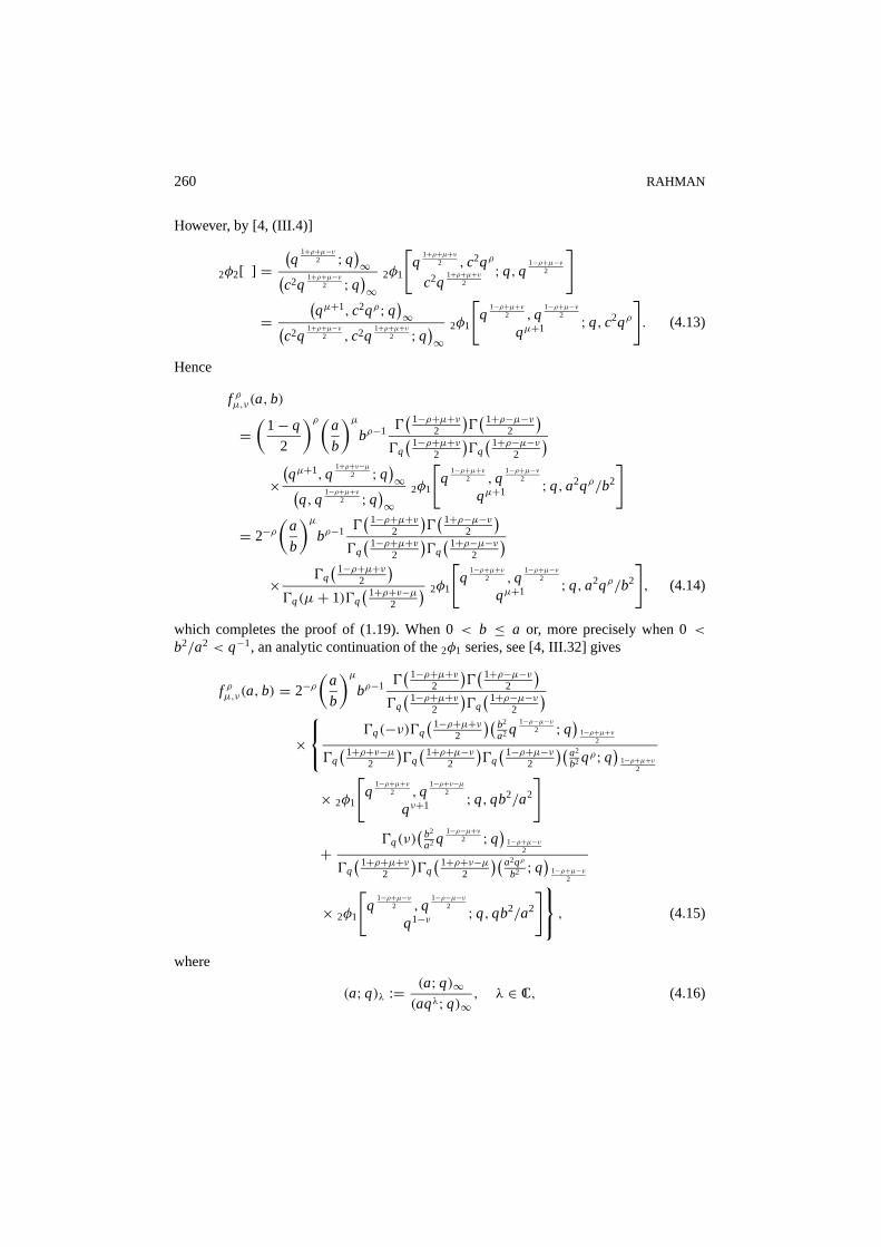
260 RAHMAN

However, by [4, (III.4)]

2φ2[ ] =(q

1+ρ+µ−ν2 ;q)∞(

c2q1+ρ+µ−ν

2 ;q)∞ 2φ1

[q

1+ρ+µ+ν2 , c2qρ

c2q1+ρ+µ+ν

2;q,q 1−ρ+µ−ν

2

]

=(qµ+1, c2qρ;q)∞(

c2q1+ρ+µ−ν

2 , c2q1+ρ+µ+ν

2 ;q)∞ 2φ1

[q

1−ρ+µ+ν2 ,q

1−ρ+µ−ν2

qµ+1 ;q, c2qρ]. (4.13)

Hence

f ρµ,ν(a, b)

=(

1− q

2

)ρ(a

b

)µbρ−1 0

( 1−ρ+µ+ν2

)0( 1+ρ−µ−ν

2

)0q( 1−ρ+µ+ν

2

)0q( 1+ρ−µ−ν

2

)×(qµ+1,q

1+ρ+ν−µ2 ;q)∞(

q,q1−ρ+µ+ν

2 ;q)∞ 2φ1

[q

1−ρ+µ+ν2 ,q

1−ρ+µ−ν2

qµ+1 ;q,a2qρ/b2

]

= 2−ρ(

a

b

)µbρ−1 0

( 1−ρ+µ+ν2

)0( 1+ρ−µ−ν

2

)0q( 1−ρ+µ+ν

2

)0q( 1+ρ−µ−ν

2

)× 0q

( 1−ρ+µ+ν2

)0q(µ+ 1)0q

( 1+ρ+ν−µ2

) 2φ1

[q

1−ρ+µ+ν2 ,q

1−ρ+µ−ν2

qµ+1 ;q,a2qρ/b2

], (4.14)

which completes the proof of (1.19). When 0< b ≤ a or, more precisely when 0<b2/a2 < q−1, an analytic continuation of the2φ1 series, see [4, III.32] gives

f ρµ,ν(a, b) = 2−ρ(

a

b

)µbρ−1 0

( 1−ρ+µ+ν2

)0( 1+ρ−µ−ν

2

)0q( 1−ρ+µ+ν

2

)0q( 1+ρ−µ−ν

2

)× 0q(−ν)0q

( 1−ρ+µ+ν2

)(b2

a2 q1−ρ−µ−ν

2 ;q) 1−ρ+µ+ν2

0q( 1+ρ+ν−µ

2

)0q( 1+ρ+µ−ν

2

)0q( 1−ρ+µ−ν

2

)(a2

b2 qρ;q) 1−ρ+µ+ν2

× 2φ1

[q

1−ρ+µ+ν2 ,q

1−ρ+ν−µ2

qν+1 ;q,qb2/a2

]

+0q(ν)

(b2

a2 q1−ρ−µ+ν

2 ;q) 1−ρ+µ−ν2

0q( 1+ρ+µ+ν

2

)0q( 1+ρ+ν−µ

2

)( a2qρ

b2 ;q)

1−ρ+µ−ν2

× 2φ1

[q

1−ρ+µ−ν2 ,q

1−ρ−µ−ν2

q1−ν ;q,qb2/a2

] , (4.15)

where

(a;q)λ := (a;q)∞(aqλ;q)∞ , λ ∈ C, (4.16)

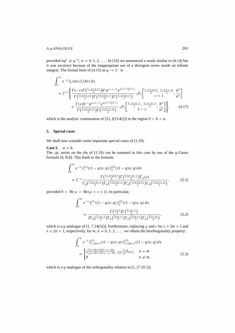
A q-ANALOGUE 261

providedaqλ 6= q−n, n = 0, 1, 2, . . . . In [16] we announced a result similar to (4.14) butit was incorrect because of the inappropriate use of a divergent series inside an infiniteintegral. The formal limit of (4.15) asq→ 1− is∫ ∞

0x−ρ Jµ(ax)Jν(bx) dx

= 2−ρ{0(−ν)0( 1−ρ+µ+ν

2

)bνaρ−ν−1 eπ i ( 1−ρ+µ+ν

2 )

0( 1+ρ+ν−µ

2

)0( 1+ρ+µ−ν

2

)0( 1−ρ+µ−ν

2

) 2F1

[ 1−ρ+µ+ν2 ,

1−ρ+ν−µ2

ν + 1; b2

a2

]

+ 0(ν)b−νaρ+ν−1 eπ i ( 1−ρ+µ−ν

2 )

0( 1+ρ+µ+ν

2

)0( 1+ρ+ν−µ

2

) 2F1

[ 1−ρ+µ−ν2 ,

1−ρ−µ−ν2

1− ν ; b2

a2

]}, (4.17)

which is the analytic continuation of [21, §13.4(2)] in the region 0< b < a.

5. Special cases

We shall now consider some important special cases of (1.19).

Case I. a = b.The 2φ1 series on the rhs of (1.19) can be summed in this case by use of theq-Gaussformula [4, II.8]. This leads to the formula∫ ∞

0x−ρ J(1)ν ((1− q)x;q)J(2)µ ((1− q)x;q) dx

= 2−ρ0( 1−ρ+µ+ν

2

)0( 1+ρ−µ−ν

2

)0q(ρ)

0q( 1+ρ−µ−ν

2

)0q( 1+ρ+µ−ν

2

)0q( 1+ρ+µ+ν

2

)0q( 1+ρ+ν−µ

2

) , (5.1)

provided 0< Reρ < Re(µ+ ν + 1). In particular,∫ ∞0

x−1J(1)ν ((1− q)x;q)J(2)µ ((1− q)x;q) dx

= 0(µ+ν

2

)0( 2−µ−ν

2

)20q

( 2−µ−ν2

)0q( 2+µ−ν

2

)0q( 2+µ−ν

2

)0q( 2+ν−µ

2

) , (5.2)

which is aq-analogue of [1, 7.14(32)]. Furthermore, replacingµ andν by λ+ 2m+ 1 andλ+ 2n+ 1, respectively, form, n = 0, 1, 2, . . . , we obtain the biorthogonality property:∫ ∞

0x−1J(1)λ+2n+1((1− q)x;q)J(2)λ+2m+1((1− q)x;q) dx

={

0(λ+2n+1)0(−λ−2n)0q(λ+2n+1)0q(−λ−2n)

1−q2(1−qλ+2n+1)

, n = m

0 n 6= m,(5.3)

which is aq-analogue of the orthogonality relation in [1, (7.10.1)].

262 RAHMAN

If, instead, we setρ = µ+ ν then we obtain the followingq-analogue of [1, 7.14(33)]:∫ ∞0

x−(µ+ν)J(1)ν ((1− q)x;q)J(2)µ ((1− q)x;q) dx

= 2−µ−νπ1/2 0(

12

)0q(µ+ ν)

0q(

12

)0q(µ+ 1

2

)0q(ν + 1

2

)0q(µ+ ν + 1

2

) , (5.4)

provided 0< Re(µ+ ν).Case II. ρ = ν − µ− 1, Re(ν − µ) > 0.In this case the2φ1 series in (4.14) becomes a1φ0 series with sum(a2/b2;q)ν−µ−1, by[4, II.3]. Thus, for 0< a < b∫ ∞

0xµ+1−ν J(1)ν (b(1− q)x;q)J(2)µ (a(1− q)x;q) dx

= 2µ+1−νaµbν−2µ−2 (a2/b2;q)ν−µ−1

0q(ν − µ)0(µ+ 1)0(−µ)0q(µ+ 1)0q(−µ), (5.5)

which gives aq-analogue of part of [1, 7.14(34)] but not the whole, i.e., it does not providean analogue of∫ ∞

0xµ+1−ν Jν(bx)Jµ(ax) dx = 0 if 0 < b < a, Re(ν − µ) > 0.

Case III. µ = ν.We have from (4.14)∫ ∞

0x−ρ J(1)ν (b(1− q)x;q)J(2)ν (a(1− q)x;q) dx

= 2−ρ(

a

b

)νbρ−1 0

(ν + 1−ρ

2

)0( 1+ρ

2 − ν)

0q(ν + 1−ρ

2

)0q( 1+ρ

2 − ν)

× 0q(ν + 1−ρ

2

)0q(ν + 1)0q

( 1+ρ2

) 2φ1

[qν+

1−ρ2 ,q

1−ρ2

qν+1 ;q, a2qρ

b2

], (5.6)

which is essentially the same as [17, (6.10)] except for a rescaling of the parameters and anapplication of the Heine transformation [4, III.2]. It follows from (5.6) that∫ ∞

0x−1J(1)ν (b(1− q)x;q)J(2)µ (a(1− q)x;q) dx

= 0(ν)0(1− ν)20q(ν + 1)0q(1− ν)

(a

b

)ν. (5.7)

A q-ANALOGUE 263

6. q-Lommel functions

The Lommel functionsµ,ν(x) is defined as a solution of the nonhomogeneous Besselequation

x2y′′ + xy′ + (x2− ν2)y = xµ+1, µ, ν unrestricted, (6.1)

and is represented by the series

sµ,ν(x) := xµ+1

(µ+ ν + 1)(µ− ν + 1)1F2

(1; µ+ ν + 3

2,µ− ν + 3

2;−x2/4

)(6.2)

providedµ± ν is not an odd negative integer, [1, 7.5(69)]. Since

sµ,ν(x) = 2µ+1∞∑

n=0

(µ+ 1+ 2n)0(µ+ 1+ n)

n![(2n+ 1+ µ)2− ν2]Jµ+1+2n(x), (6.3)

by virtue of the orthogonality property [1, (7.10.1)] that provides Neumann series expansionsof f (x) in terms ofJµ+1+2n(x) we are led to consider the series

S(z) :=∞∑

n=0

1− qµ+1+2n

1− qµ+1

(qµ+1,q

µ−ν+12 ,q

µ+ν+12 ;q)

n(a,a

µ+ν+32 ,q

µ−ν+32 ;q)

n

q(n+1

2)

× J(1)µ+1+2n(z;q). (6.4)

For |z| < 2 we find, after an interchange of the order of summation followed by an obvioustransformation, that

S(z) = (qµ+2;q)∞(q;q)∞ (z/2)µ+1

∞∑k=0

(−z2/4)k

(q,qµ+2;q)k× 6W5

(qµ+1;q µ−ν+1

2 ,qµ+ν+1

2 ,q−k;q,qk+1). (6.5)

By [4,II.21] we find the sum of the6W5 series as

(qµ+2,q;q)k(qµ+ν+3

2 ,qµ−ν+3

2 ;q)k ,

S(z) = (qµ+2;q)∞(q;q)∞ (z/2)µ+1

× 3φ2

[q, 0, 0

q,−z2/4qµ+ν+3

2 ,qµ−ν+3

2 ;]. (6.6)

264 RAHMAN

In analogy of (6.2) we now define aq-Lommel function by

sµ,ν(x;q) := (q;q)∞(qµ+2;q)∞ 2µ+1 (1− q)2

4(1− q

µ+ν+12)(

1− qµ−ν+1

2)S(x)

= xµ+1(1− q)2

4(1− q

µ+ν+12)(

1− qµ−ν+1

2)

× 3φ2

[q, 0, 0

q,−x2/4qµ+ν+3

2 ,qµ−ν+3

2 ;]. (6.7)

which is aq-analogue of (6.2) in the sense that

limq→1−

sµ,ν((1− q)x;q) = sµ,ν(x). (6.8)

It can be shown in a straightforward manner thatsµ,ν(x;q) satisfies theq-differenceequation

sµ,ν(qx;q)− (qν/2+ q−ν/2)sµ,ν(q1/2x;q)+ (1+ x2/4)sµ,ν(x;q) =(

1− q

2

)2

xµ+1,

(6.9)

where the corresponding homogeneous equation is satisfied byJ(1)ν (x;q), see [8].Theq-Newmann series for a functionf (x) can be written, formally, in the form

f (x) =∞∑

n=0

an J(2)ν+1+2n((1− q)x;q), (6.10)

where

an = 0q(ν + 1)0q(−ν)0(ν + 1)0(−ν) qn(2ν+1+2n) 2(1− qν+1+2n)

(1− q)

×∫ ∞

0x−1J(1)ν+1+2n((1− q)x;q) dx, (6.11)

by virtue of (5.3).In particular, by integrating∫ ∞

0xρ−1J(1)ν+1+2n((1− q)x;q) dx

with the help of (1.13) and the Ramanujan integral [18] we find, after some simplifications,the following expansion

(x/2)ρ = 0q(ν + 1)0q(−ν)0(ν + 1)0(−ν)

0(ν+ρ+1

2

)0( 1−ν−ρ

2

)0q(ν−ρ+3

2

)0q( 1−ν−ρ

2

)×∞∑

n=0

1− qν+1+2n

1− qν+1

(qν+ρ+1

2 ;q)n(

qν−ρ+3

2 ;q)n

qn(2ν+1+2n) (6.12)

× J(2)ν+1+2n((1− q)x;q).

A q-ANALOGUE 265

References

1. A. Erdelyi, W. Magnus, F. Oberhettinger, and F.G. Tricomi (ed.),Higher Transcendental Functions, Vol II,McGraw-Hill, New York, 1953.

2. H. Exton, “A basic analogue of the Bessel-Clifford equation,”Jnanabha8 (1978) 49–56.3. H. Exton,q-Hypergeometric Functions and Applications, Ellis Horwood, 1983.4. G. Gasper and M. Rahman,Basic Hypergeometric Series, Cambridge University Press, 1990.5. W. Hahn, “Beitrage zur theorie der Heineschen Reichen,”Math. Nachr.2 (1949) 340–379.6. W. Hahn, “Die mechanische Deutung einer geometrischen Differenzgleichung,”Z. Angew. Math. Mech.33

(1953) 270–272.7. M.E.H. Ismail, “The basic Bessel functions and polynomials,”SIAM J. Math. Anal.12 (1981) 454–468.8. M.E.H. Ismail, “The zeros of basic Bessel functions, the functionsJν+ax(x) and the associated orthogonal

polynomials,”J. Math. Anal. Appl.86 (1982) 1–19.9. M.E.H. Ismail, “Some properties of Jackson’s thirdq-Bessel function,” to appear.

10. M.E.H. Ismail, D. Masson, and S.K. Suslov, “Theq-Bessel functions on a quadratic grid,”Algebraic Methodsand q-Special Functions(Montreal, 1996) 183-200, CRM Lecture Notes 22, Amer. Math. Soc., Providence,RI, 1999.

11. M.E.H. Ismail, D. Masson, and S.K. Suslov, “Properties of aq-analogue of Bessel functions,” to appear.12. F.H. Jackson, “On generalized functions of Legendre and Bessel,”Trans. Roy. Soc. Edin.41 (1904) 1–28.13. F.H. Jackson, “Applications of basic numbers to Bessel’s and Legendre’s functions,”Proc. Lond. Math. Soc.

2(2) (1905) 192–220.14. H.T. Koelink, “The quantum group of plane motions and basic Bessel functions,”Indag. Mathem., N.S.6(2)

(1995) 197–211.15. T.H. Koornwinder and R.F. Swarttouw, “Onq-analogues of the Fourier and Hankel transforms,”Trans. Amer.

Math. Soc.333(1992) 445–461.16. M. Rahman, “Some infinite integrals ofq-Bessel functions,”Ramanujan International Symposium on Analysis,

Proceedings of Ramanujan Birth Centenary Year: Pune, India, N. K. Thakore, ed. 1987, pp. 117–138.17. M. Rahman, “An addition theorem and some product formulas forq-Bessel functions,”Can. J. Math.40

(1988) 1203–1221.18. S. Ramanujan, “Some definite integrals,”Mess. Math.44 (1915) 10–18; reprinted in Collected papers of

Srinivasa Ramanujan (G.H. Hardy, P.V. Seshu Aiyer, and B.M. Wilson, eds.), Cambridge University Press,1927; reprinted by Chelsea, New York, 1962.

19. S.K. Suslov, “Some orthogonal very-well-poised8φ7 functions that generalize Askey-Wilson polynomials,”MSRI Preprint#1997-060, Berkeley, California, 1997.

20. R.F. Swarttouw, “The Hahn-Extonq-Bessel Functions,” Ph.D. Thesis, Delft Technical University, 1992.21. G.N. Watson, “Theory of Bessel Functions,” Cambridge University Press, 1944.