A Comprehensive Study on Multiphase Flow through Pipeline ...

A Comprehensive Study on Multiphase Flow through Pipeline and Annuli using CFD

Approach

by

© Rasel A Sultan

A Thesis submitted to the

School of Graduate Studies

in partial fulfilment of the requirements for the degree of

Master of Engineering

Faculty of Engineering and Applied Science

Memorial University of Newfoundland

May 2018

St. John’s Newfoundland

ii

Abstract

The physical phenomenon of more than one state or phase (i.e. gas, liquid or solid) simultaneously

flowing is defined as multiphase flow. The overall performance of multiphase flow is more

complex compared to single phase flow through pipeline or annuli. Calculation accuracy of

pressure drop, and particle concentration is very important to design pipeline or annular geometry

for multiphase flow. The objectives in the present study are to design a CFD model that can be

used to predict multiphase fluid flow properties with more accuracy; to validate proposed CFD

model with experimental data and existing empirical correlations at different orientations of

geometry and combination of fluids; and to investigate the effects of pipe diameter, wall

roughness, fluid velocity, fluid type, particle size, particle concentration, drill pipe rotation speed

and drill pipe eccentricity on pressure losses and settling conditions. Three distinct phases of

working fluids are used to fulfill the project. Simulation process is conducted using ANSYS fluent

version 16.2 platform. Eulerian model with Reynolds Stress Model (RSM) turbulence closure is

selected as optimum to analyze multiphase fluid flow. Pressure gradient and sand concentration

profile are the primary output parameters to analyze. This article combines validation work at all

possible cases to verify the developed model and parametric study to observe the effects of selected

parameters on particle deposition. In parametric analysis, eccentricity of the annular pipe is varied

from 0 – 50% and rotated about its own axis from 0 – 150 rpm. The diameter ratio of the simulated

annuli is 0.56. Results show very good agreement with existing experiments and developed

correlations. Also, the effects of different parameters are briefly analyzed with proper

explanations. Fluid Structure Interaction (FSI) is introduced to observe the fluid flow effect on

pipeline deformation.

iii

Acknowledgement

First and foremost, I am very grateful to my supervisor Dr. Mohammad Azizur Rahman, co-

supervisors Dr. Sohrab Zendehboudi and Dr. Vassilios C. Kelessidis, for the continuous support,

guidance, and encouragement they gave me and also for the financial support provided. I

acknowledge with gratitude the valuable suggestions and feedback in preparation of the

manuscripts given by Dr. Vandad Talimi from C-Core Canada and Dr. M M A Rushd from Texas

A&M University at Qatar. Also, I greatly acknowledge the funding received by Natural Science

and Engineering Research Council (NSERC) of Canada, Research and Development Corporation

Newfoundland and Labrador (RDC, newly called InnovateNL) and School of Graduate Studies

(SGS) of Memorial University.

Furthermore, I highly appreciate the support given by the research and administration staff of the

Faculty of Engineering and Applied Science, Memorial University. Especially Dr. Faisal Khan,

Dr. Leonard Lye, Moya Crocker, Colleen Mahoney, and everyone who helped me in some way.

My heartfelt thanks also go to all my friends and colleagues for their continuous support from the

beginning, specially Mohammad Masum Jujuly who supported me to learn ANSYS software.

Finally, I would like to thank my mother Aleya Begum, my father Mohammed Tipu Sultan and

my sister Rahana Sultana for all the love and support. Thank you.

iv

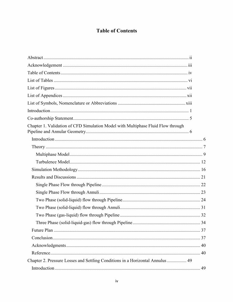
Table of Contents

Abstract ............................................................................................................................... ii

Acknowledgement ............................................................................................................. iii

Table of Contents ............................................................................................................... iv

List of Tables ..................................................................................................................... vi

List of Figures ................................................................................................................... vii

List of Appendices ............................................................................................................ xii

List of Symbols, Nomenclature or Abbreviations ........................................................... xiii

Introduction ......................................................................................................................... 1

Co-authorship Statement ..................................................................................................... 5

Chapter 1. Validation of CFD Simulation Model with Multiphase Fluid Flow through

Pipeline and Annular Geometry .......................................................................................... 6

Introduction ................................................................................................................................. 6

Theory ......................................................................................................................................... 7

Multiphase Model .................................................................................................................... 9

Turbulence Model .................................................................................................................. 12

Simulation Methodology ........................................................................................................... 16

Results and Discussions ............................................................................................................ 21

Single Phase Flow through Pipeline ...................................................................................... 22

Single Phase Flow through Annuli ........................................................................................ 23

Two Phase (solid-liquid) flow through Pipeline .................................................................... 24

Two Phase (solid-liquid) flow through Annuli ...................................................................... 31

Two Phase (gas-liquid) flow through Pipeline ...................................................................... 32

Three Phase (solid-liquid-gas) flow through Pipeline ........................................................... 34

Future Plan ................................................................................................................................ 37

Conclusion ................................................................................................................................. 37

Acknowledgments ..................................................................................................................... 40

Reference ................................................................................................................................... 40

Chapter 2. Pressure Losses and Settling Conditions in a Horizontal Annulus ................. 49

Introduction ............................................................................................................................... 49

v

Literature Review ...................................................................................................................... 50

Methods ..................................................................................................................................... 51

CFD Simulation ..................................................................................................................... 51

Turbulence Model Selection .................................................................................................. 54

Length Independence Study .................................................................................................. 59

Mesh analysis ........................................................................................................................ 60

CFD Model Validation .............................................................................................................. 62

Single Phase Flow through Annuli ........................................................................................ 62

Two Phase (solid-liquid) flow through Annuli ...................................................................... 64

Results and Discussion .............................................................................................................. 65

Effect of Flow Rate ................................................................................................................ 66

Effect of Drill Pipe Rotation and Eccentricity ....................................................................... 71

Effect of Particle Size ............................................................................................................ 72

Conclusions ............................................................................................................................... 73

References ................................................................................................................................. 74

Chapter 3. CFD Simulation of Three Phase Gas-Liquid-Solid Flow in

Horizontal Pipes ................................................................................................................ 80

Introduction ............................................................................................................................... 81

Mathematical Model ................................................................................................................. 82

Simulation Methodology ........................................................................................................... 88

Simulation Validation ............................................................................................................... 89

Parametric Sensitivity Study ..................................................................................................... 92

Conclusion ................................................................................................................................. 98

References ................................................................................................................................. 99

Summary ......................................................................................................................... 106

Appendices ...................................................................................................................... 108

vi

List of Tables

Tables in Chapter 1

Table 1. Variable Parameter Ranges………………………………………………… 21

Tables in Chapter 2

Table 1. Analysis of Turbulence Model Performance………………………………… 55

Tables in Chapter 3

Table 1. Mesh Distribution Statistics…………………………………………………. 88

vii

List of Figures

Figures in Chapter 1

Figure 1. Presentation of the comparative analysis of different turbulence models: (a)

Kelessidis et al., 2011, (b) Skudarnov et al., 2004…………………………………….

14

Figure 2. Presentation of Mesh Independence from Fukuda and Shoji, 1986………… 17

Figure 3. Mesh distribution in (a) pipe geometry, (b) annular geometry……………… 19

Figure 4. Pressure Gradient variation along pipe length……………………………… 20

Figure 5. Optimum convergence rate analysis from Camçi, 2003……………………. 20

Figure 6. Comparison of simulated pressure gradient with Wood (1966) correlation,

experimental data from Kaushal et al. (2005) and Skudarnov et al. (2004) at different

inlet velocity…………………………………………………………………………..

22

Figure 7. Comparison of simulated pressure gradient with Haaland (1983) correlation

and experimental data from Kelessidis et al. (2011) and Camçi (2003) at different inlet

velocity………………………………………………………………………………...

24

Figure 8. Particle size distribution of different particle used in Kaushal et al. (2005)... 26

Figure 9. Comparison of simulated pressure gradient with experimental data from

Skudarnov et al. (2001), Kaushal et al. (2005) and Skudarnov et al. (2004) at different

inlet slurry velocity……………………………………………………………………

27

Figure 10. Comparison of simulated solid local volumetric concentration across

vertical centerline with Gillies and Shook, 1994………………………………………

28

Figure 11. Comparison of simulated and measured solid local volumetric

concentration across vertical centerline with Roco and Shook, 1983………………….

29

viii

Figure 12. Particle size distribution of different particle used in Roco and Shook

(1983)……………………………………………………………………………........

30

Figure 13. Solid concentration distribution in the vertical cross section plane (data

from Roco and Shook, 1983)………………………………………………………….

31

Figure 14. Comparison of simulated two-phase frictional pressure gradient at different

mixture velocity and volume concentration of slurry with Ozbelge and Beyaz,

2001…………………………………………………………………………................

32

Figure 15. Comparison of simulated axial liquid velocity at vertical position with

experimental data from Kocamustafaogullari and Wang, 1991……………………….

33

Figure 16. Comparison of simulated axial liquid velocity at horizontal position with

experimental data from Kocamustafaogullari and Wang, 1991……………………….

34

Figure 17. Comparison of simulated pressure gradient as a function of gas velocity

with experimental data from Fukuda and Shoji, 1986…………………………………

35

Figure 18. Comparison of simulated pressure gradient as a function of gas volume

fraction with Gillies et al., 1997……………………………………………………….

36

Figure 19. Particle size distribution of different particle used in Fukuda and Shoji

(1986)…………………………………………………………………………………..

37

Figure 20. Overall simulation predictions of different experiment data………………. 39


Figure 1. Performance of turbulence models in predicting pressure loss (Data Source:

Kaushal et al., 2005)…………………………………………………………………...

54

ix

Figure 2. Length independence analysis (A) 75% eccentric, 150 RPM inner pipe

rotation speed and 400 kg/min flow rate; (B) Concentric, stationary inner pipe and 200

kg/min flow rate……………………………………………………………………….

59

Figure 3. Mesh distribution…………………………………………………………… 61

Figure 4. Mesh independence analysis…………….………………………………….. 61

Figure 5. An example of optimum convergence rate analysis………………………… 62

Figure 6. Comparison of simulated pressure gradient with Haaland (1983) correlation

and experimental data from Kelessidis et al. (2011) and Camçi (2003) at different inlet

velocity…………………………………………………………………………………

63

Figure 7. Comparison of simulated two-phase frictional pressure gradient at different

mixture velocity and volume concentration of slurry with Ozbelge and Beyaz, 2001…

65

Figure 8. Effect of fluid flow on particle concentration profile (Concentric annuli with

stationary inner pipe)…………………………………………………………………..

66

Figure 9. Effect of fluid flow on particle concentration profile (Concentric annuli with

150 rpm rotating inner pipe)……………………………………………………………

67

Figure 10. Effect of fluid flow on particle concentration profile (50% eccentric annuli

with stationary inner pipe)……………………………………………………………..

67

Figure 11. Effect of fluid flow on particle concentration profile (50% eccentric annuli

with 150 rpm inner pipe)………………………………………………………………

68

Figure 12. Contour distribution of sand concentration profile: (a) Re = 4*104, (b) Re =

7*104, (c) Re = 105 and (d) Re = 2*105……………………………………………….

70

Figure 13. Effect of inner pipe rotation on pressure loss……………………………… 71

x

Figure 14. Effect of inner pipe eccentricity on pressure loss at different rotational

speed……………………………………………………………………………………

72

Figure 15. Effect of sand particle size on bed concentration near wall………………... 73


Figure 1. Optimum turbulence model analysis………………………………………… 85

Figure 2. Mesh distribution in the pipe geometry……………………………………... 88

Figure 3. Optimum convergence rate analysis………………………………………… 89

Figure 4. Comparison of simulation data with correlations (Wood, 1966) and

experimental data of Skudarnov et al. (2004)………………………………………….

90

Figure 5. Comparison of pressure gradient as a function of gas velocity with 24.7%

solid volume concentration in slurry (Cv) and 3 m/s slurry velocity…………………...

91

Figure 6. Pressure Gradient at different gas velocity and solid volume concentration in

slurry with other variables constant……………………………………………….........

92

Figure 7. Sand concentration distribution in vertical plane at outlet with 1.14 m/s air

inlet. (a) Cv = 8.8% and (b) Cv = 13.3%..........................................................................

94

Figure 8. Sand concentration distribution in vertical plane at outlet with Cv = 24.7%.

(a) 0.643 m/s air inlet, (b) 1.36 m/s air inlet and (c) 1.9 m/s air inlet…………………...

95

Figure 9. Pressure Gradient at different gas velocity and pipe diameter with other

variables constant………………………………………………………………………

96

Figure 10. Pressure Gradient at different gas velocity and pipe wall roughness with

other variables constant………………………………………………………………...

96

xi

Figure 11. Pressure Gradient at different gas velocity and water viscosity with other

variables constant………………………………………………………………………

97

Figure 12. Contour of pipeline deformation………………………………………….... 99

xii

List of Appendices

Appendix 1. Sensitivity Analysis of A CFD Model for Simulating Slurry Flow

Through Pipeline……………………………………………………………………...

108

Appendix 2. A Computational Fluid Dynamics Study of Two-Phase Slurry and Slug

Flow in Horizontal Pipelines………………………………………………………….

139

Appendix 3. CFD and Experimental Approach on Three Phase Gas-Liquid-Solid

Newtonian Fluid flow in Horizontal Pipes…………………………………………….

152

Appendix 4. Data Tables……………………………………………………………... 173

xiii

List of Symbols, Nomenclature or Abbreviations

CFD Computational Fluid Dynamics

RSM Reynolds Stress Model

SST Shear Stress Transport

RANS Reynolds Averaged Navier–Stokes

LES Large Eddy Simulation

FSI Fluid Structure Interaction

SIMPLE Semi-Implicit Method for Pressure Linked Equations

ANN Artificial Neural Network

dm Sand Particle Diameter

Cv Sand Volumetric Concentration

D Pipe Diameter

Dh Hydraulic Diameter

da Air Bubble Diameter

Ca Air Volumetric Concentration

v Fluid Velocity

va Air Velocity

vw Water Velocity

vs Sand Velocity

휀 Wall Roughness

𝑅𝑒 Reynolds Number

𝑓 Friction Factor

1

Introduction

The use of multiphase flow like liquid-gas, liquid-solid and even solid-liquid-gaseous three-phase

flow through pipeline or annuli is increasing every day. Flow through pipeline and annular pipe

makes it simpler to transport required materials to destined places. The overall performance of

multiphase flow is more complex compared to single phase flow as this flow must combat various

problems such as corrosion, erosion, slugging etc. to get optimum result. Also, the chemical and

physical interactions between phases, non-linearity of governing equations compared to the single

phase flow, large variations in flow characteristics with respect to process and operating conditions

are the main challenges while studying multiphase flow and designing the corresponding

equipment. This complexity presents a major challenge in the study of multiphase flows and a lot

more extravagant researches are required before even a shallow understanding is achieved.

Applications of this research work with multiphase flow through pipeline or annuli can be listed

as below –

Transportation of Raw Materials, Wastes and Sludge.

Mining Plants.

Coal Processing Plants.

Food and Chemical Plants.

Petroleum Industries (oil and gas transportation & oil and gas or oil and sand production in

pipelines or production wells where the pressure drop and temperature change are not that

much significant.)

Nuclear Plants.

2

Power Plants.

Biomedical Engineering Applications.

Micro-Scale Fluid Dynamics Studies.

The existing empirical correlations become less accurate as those involve many simplifying

assumptions. CFD simulations help to minimize such kind of assumptions. More limitations found

from literature reviews are –

• Developed empirical correlations along with experimental studies of two and three phase flow

in pipeline and annuli are based on limited scopes, data and application ranges (Hernández et

al., 2008 and Rahman et al., 2013).

• CFD approaches are not validated and acceptable in wide range of operating conditions. In

most of the previous CFD studies, the numerical model is validated using a very limited

number of data sets (for example, Dewangan and Sinha, 2016, Chen et al., 2009 and Kumar

and Kaushal, 2016).

In this study a CFD model is developed by using Navier Stokes equations to model the

hydrodynamics of the flow system. Present work is focused on developing a CFD model capable

of taking into consideration the effects of all important multiphase flow parameters, such as fluid

velocity, fluid type, particle size, particle concentration, annular pipe rotational speed and annular

pipe eccentricity. Before conducting parametric study, our model is validated with twelve different

experimental data sets which involve flow conditions significantly different from each other.

Objectives of the present work are:

3

To develop a CFD model which will be highly reliable to researchers and engineers at different

applications and different conditions related to pipeline or annular pipe flow with multiphase

fluids.

To validate the model with wide ranges of experimental and empirical data sets.

To conduct parametric study with developed CFD model to predict frictional pressure loss and

settling conditions through annular pipe.

To analyze the validity of the developed model with three phase gas-liquid-solid flow through

pipeline and introduce Fluid Structure Interaction (FSI) for further research.

This thesis is written in manuscript format and is divided into three main chapters excluding the

introduction and summary. Appendices are added which include related published works and data

tables. The following paragraphs briefly shows outline the chapters.

Chapter 1 is on extensive literature reviews and validation processes of our developed CFD model

at different operating conditions with multiphase fluid flow through pipeline and annuli. Twelve

different data sources are used to validate our developed model. Comprehensive theoretical

analysis is also done to explain the proposed model and its validity. This chapter is submitted in

Particulate Science and Technology journal and received a minor review. The chapter is updated

according to the received reviews.

Chapter 2 is on analyzing frictional pressure loss and settling conditions through annular pipe.

Finding ‘deposition velocity’ is the main goal of this chapter. Effect of fluid velocity, fluid type,

particle size, particle concentration, annular pipe rotational speed and annular pipe eccentricity on

pressure gradient and particle deposition are studied for a wide range of conditions. Few results

are discussed and all findings are shared for further investigation. This chapter is projected to

submit in SPE Drilling & Completion Journal.

4

Chapter 3 is on three phase gas-liquid-solid flow in horizontal pipes using developed CFD model.

Three phase flow analysis is very rare and new in multiphase flow research area. Our model shows

very good agreement with three phase experimental data and thus we approached three phase flow

analysis showing few findings from our model. Fluid Structure Interaction (FSI) is discussed

which eventually will lead to find several hazards (e.g. pipe deformation, leakage, fire explosions,

material losses etc.) due to multiphase fluid flow through pipeline and annuli. This chapter is

accepted and presented at ASME 2017 Fluids Engineering Division Summer Meeting

(FEDSM2017).

In Summary section, the outcomes are presented, and future recommendations are suggested.

Appendix 1, 2 and 3 present published works related to the chapters. Appendix 1 is accepted and

presented at International Conference on Petroleum Engineering 2016 (ICPE-2016) where two

phase slurry flow through pipeline is analyzed. Appendix 2 is accepted and will be presented at 3rd

Workshop and Symposium on Safety and Integrity Management of Operations in Harsh

Environments (C-RISE3) where two phase slug flow is analyzed with FSI concept. Appendix 3 is

accepted in International Journal of Computational Methods and Experimental Measurements (in

press) where experimental approach with our developed model is discussed. Appendix 4 presents

data tables from parametric analysis.

5

Co-authorship Statement

In all the papers presented in the following chapters, myself, Rasel A Sultan, is the principle author.

My supervisor Dr. Mohammad Azizur Rahman, co-supervisors Dr. Sohrab Zendehboudi, and Dr.

Vassilios C. Kelessidis provided theoretical and technical guidance, support with analysis,

reviewing and revising of the manuscripts. I have carried out most of the data collection and

analysis. I have prepared the first drafts of the manuscripts and subsequently revised the

manuscripts based on the co-authors’ feedback and the peer review process. Co-authors and

supervisors assisted in developing the concepts and testing of the models. As co-authors, Dr.

Vandad Talimi, Dr. M M A Rushd, Dr. John Shirokoff, Hassn Hadia and Serag Alfarek contributed

through support in development of model, introducing experimental setup, reviewing and revising

the manuscripts.

6

Chapter 1. Validation of CFD Simulation Model with Multiphase Fluid Flow

through Pipeline and Annular Geometry

Rasel A Sultan1, M. A. Rahman2, Sayeed Rushd2, Sohrab Zendehboudi1, Vassilios C. Kelessidis3

1Faculty of Engineering and Applied Science, Memorial University of Newfoundland, Canada

2Texas A&M University at Qatar, Doha, Qatar

3Petroleum Institute, Abu Dhabi, UAE

Abstract

Accuracy of prediction of pressure losses plays a vital role in the design of multiphase flow

systems. The present study focused on the development of a computational fluid dynamics (CFD)

model to predict these parameters conveniently and accurately. The main objective was to validate

the developed model through comparison of its simulation results with existing experimental data

and empirical correlations. Both pipeline and annular geometries were considered for the

validation. A number of datasets that involved a significant variation in process conditions were

used for the validation. All three phases—liquid (water), gas (air), and solid (sand)—were taken

into account. The simulations were conducted using the workbench platform of ANSYS Fluent

16.2. The Eulerian model of multiphase flow and the Reynolds stress model (RSM) of turbulence

closure available in this version of Fluent were used for the present study. The average velocities

and volumetric concentrations of involved phases were specified as the inlet boundary conditions.

The stationary surfaces of the flow channels were hydrodynamically considered as either smooth

or rough walls, and the outlets were regarded as being open to the atmosphere. The simulation

results of pressure loss showed good agreement with the corresponding measured values as well

as with the predictions of well-established correlations.

7

Introduction

Multiphase flows in pipelines or annuli are of great importance and widely employed in various

industries and applications, such as chemical process and petroleum industries, nuclear plants,

pipeline engineering, power plants, biomedical engineering, microscale fluid dynamics studies,

mining plants, food processing industries, geothermal flows, and extrusion of molten plastics

(Roco and Shook, 1983; Dewangan and Sinha, 2016). In particular, slurry flow or solid–liquid

two-phase flow has become increasingly popular owing to its manifold applications in various

industries. This kind of two-phase flow through a pipeline is being studied since the third decade

of the 20th century with focus on the development of general solutions based on available

experimental data for solid volumetric or mass concentration profiles, pressure drops, and slurry

velocity profiles. Among the initial studies, those of O’Brien and Morrough (1933) and Rouse

(1937) focused on slurry flows in an open channel with low solid concentrations. They used a

diffusion model to predict the concentration distribution. Durand (1951), Durand and Condolios

(1952), and Newitt et al. (1955) are also considered as pioneers in describing the frictional pressure

losses in slurry flow. Correlations established by Thomas (1965) and Krieger (1972) for

homogeneous slurry and the model proposed by Ling et al. (2003) for heterogeneous slurry

provided a new dimension to the study of pressure losses in this kind of multiphase flow. Some

other important works on empirical correlations for slurry pressure losses include those of Govier

and Aziz (1972), Vocadlo and Charles (1972), Aude et al. (1974), Aude et al. (1975), and Seshadri

(1982). It is important to note that most of the studies conducted prior to 2000 had a limited

application range, scope, and data (Lahiri and Ghanta, 2007). Different computational fluid

dynamics (CFD)-based models were proposed later in an effort to address these limitations. A

number of such studies were conducted on slurry flow in a pipeline (Ling et al., 2003; Cornelissen

8

et al., 2007; Hernández et al., 2008; Lin and Ebadian, 2008; Chen et al., 2009; Kaushal et al., 2013;

Gopaliya and Kaushal, 2015; Kumar and Kaushal, 2016). However, the outcomes of studies on

pipeline slurry flows are not necessarily applicable to similar flows in annuli. Annular slurry flows

have not been studied as extensively as the counterpart flows in pipeline. Some remarkable works

on annular slurry flows include those of Özbelge and Köker (1996), Özbelge and Beyaz (2001),

Eraslan and Özbelge (2003), Özbelge and Eraslan (2006), Camçi and Özbelge (2006), Kelessidis

et al. (2007), and Özbelge and Ünal (2008). Furthermore, Escudier et al. (2002) presented a

bibliographic list of works on annular flows.

Govier and Aziz (1972) well presented two-phase flow of liquid and gas in a pipeline. Addition of

solid particles to the two-phase pipeline flow was found to lead to a reduction in the pump size

and an increase in the flow rate (Orell, 2007; Pouranfard et al., 2015). This kind of three-phase

system helps to reduce air pollution, noise, and accidents and also provides energy savings.

Addition or injection of air in a two-phase slurry system was also reported to reduce pumping cost

and enhance bitumen recovery from oil-sand fields (Sanders et al., 2007). Numerous studies were

conducted on three-phase pipeline flow (Scott and Rao, 1971; Toda et al., 1978, Hatate et al., 1986;

Fukuda and Shoji, 1986; Kago et al., 1986; Gillies et al., 1997; Bello et al., 2005; Rahman et al.,

2013; Li et al., 2015; Pouranfard et al., 2015). Most of these studies were experimental works that

focused on measurement of frictional pressure losses, deposition velocity (i.e., the minimum

superficial velocity of a mixture to prevent accumulation of solids or wastes in the pipeline), and

in situ concentration of each phase. Despite being many in number, these experimental works

cover a narrow range of operating conditions (Orell, 2007; Rahman et al., 2013). Research works

based on CFD or numerical simulation are a new addition in this field. A few notable examples of

9

such works include those of Van Sint Annaland et al. (2005), Washino et al. (2011), Baltussen et

al. (2013), and Liu et al. (2015).

In the present study, a CFD model is used to simulate multiphase fluid flows through pipelines and

annuli. The model is validated through comparison of its simulation results with experimental data

of one-, two-, and three-phase flows. In most of the previous CFD studies, the numerical model

was validated using a very limited number of datasets; the number of datasets was typically as low

as one or two (see, for example, Dewangan and Sinha (2016), Chen et al. (2009), and Kumar and

Kaushal (2016)). In contrast, our modeling approach is validated through comparison with 12

different experimental datasets involving flow conditions that are significantly different from each

other. The CFD results are also compared with the predictions of well-established correlations. In

view of the fact that process conditions vary over a wide span in the industry, the objective of the

present study is to verify the suitability of a commercially available CFD model to simulate

multiphase flows in both pipelines and annuli under a wide range of process conditions.

Theory

Multiphase Model

The Eulerian model based on the Euler-Euler approach is used in the present CFD study as the

multiphase model (Fluent, 2009). This is because this investigation includes solid–liquid–gas

three-phase flows, in which both granular (fluid–solid) and non-granular (fluid–fluid) flows are

involved. The Eulerian model is known to be capable of addressing different kinds of couplings

with individual momentum and continuity equations quite effectively (Anderson and Jackson,

1967).

Volume fractions represent the space occupied by each phase, and the laws of conservation of

mass and momentum are satisfied by each phase individually. The conservation equations can be

10

derived by averaging the local instantaneous balance for each of the phases (Anderson and

Jackson, 1967) or by using the mixture theory approach (Bowen, 1976).

The volume of phase 𝑞, 𝑉𝑞, is defined by

𝑉𝑞 = ∫ 𝑎𝑞𝑑𝑉 (1)

where,

𝑎𝑞 = volume fraction

and ∑ 𝑎𝑞 = 1𝑛𝑞=1 (2)

Continuity equation for mixture is as below -

𝜕

𝜕𝑡(𝑎𝑞𝜌𝑞) + ∇. (𝑎𝑞𝜌𝑞𝜗𝑞 ) = 0 (3)

where, 𝜌𝑞 is the phase reference density, or the volume averaged density of the 𝑞𝑡ℎ phase in the

solution domain. 𝜗𝑞 indicates velocity vector.

The conservation of momentum for a fluid phase 𝑞 is –

𝜕

𝜕𝑡(𝑎𝑞𝜌𝑞𝜗𝑞 ) + ∇. (𝑎𝑞𝜌𝑞𝜗𝑞 𝜗𝑞 ) = −𝑎𝑞∇p + ∇. 𝜏 + 𝑎𝑞𝜌𝑞𝑔 + ∑ 𝐾𝑝𝑞(𝜗𝑝 − 𝜗𝑞 ) +

𝑛𝑝=1

𝑝𝑞𝜗𝑝𝑞 − 𝑞𝑝𝜗𝑞𝑝 + (𝐹𝑞 + 𝐹 𝑙𝑖𝑓𝑡,𝑞 + 𝐹 𝑣𝑚,𝑞) (4)

Here 𝑔 is the acceleration due to gravity, 𝜏 is the 𝑞𝑡ℎ phase stress-strain tensor, 𝐹𝑞 is an external

body force, 𝐹 𝑙𝑖𝑓𝑡,𝑞 is a lift force and 𝐹 𝑣𝑚,𝑞 is a virtual mass force.

11

Considering the work of Alder and Wainwrigh (1960), Chapman and Cowling (1970) and Syamlal

et al. (1993), a multi-fluid granular model is used to describe the flow behavior of a fluid-solid

mixture.

The conservation of momentum for the solid phase is -

𝜕

𝜕𝑡(𝑎𝑠𝜌𝑠𝜗𝑠 ) + ∇. (𝑎𝑠𝜌𝑠𝜗𝑠 𝜗𝑠 ) = −𝑎𝑠∇p − ∇𝑝𝑠 + ∇. 𝜏 + 𝑎𝑠𝜌𝑠𝑔 + ∑ 𝐾𝑙𝑠(𝜗𝑙 − 𝜗𝑠 ) +

𝑁𝑙=1

𝑙𝑠𝜗𝑙𝑠 − 𝑠𝑙𝜗𝑠𝑙 + (𝐹𝑠 + 𝐹 𝑙𝑖𝑓𝑡,𝑠 + 𝐹 𝑣𝑚,𝑠) (5)

where, 𝑝𝑠 is the 𝑠𝑡ℎ solids pressure, 𝐾𝑙𝑠 = 𝐾𝑠𝑙 is the momentum exchange coefficient between

fluid or solid phase 𝑙 and solid phase 𝑠, 𝑁 is the total number of phases.

For granular flows, the solids pressure is composed of a kinetic term and a second term due to

particle collisions –

𝑝𝑠 = 𝑎𝑠𝜌𝑠𝛩𝑠 + 2𝜌𝑠(1 + 𝑒𝑠𝑠)𝑎𝑠2𝑔0,𝑠𝑠𝛩𝑠 (6)

where 𝑒𝑠𝑠 is the coefficient of restitution for particle collisions, 𝑔0,𝑠𝑠 is the radial distribution

function and 𝛩𝑠 is the granular temperature. A default value of 0.9 for 𝑒𝑠𝑠 is used but the value can

be adjusted for different particle type. This value is selected based on Fluent (2009) and a trial &

error process during validation. The function 𝑔0,𝑠𝑠 is a distribution function that control the

transition from the compressible condition to incompressible condition. A value of 0.63 is the

default for 𝑎𝑠,𝑚𝑎𝑥.

Equation 7 is showing the form of the coefficient of restitution (Wakeman and Tabakoff, 1982).

𝑒𝑠𝑠 =𝑣2

𝑣1 (7)

where 𝑣2 = particle velocity after collision, and 𝑣1 = particle velocity before collision.

12

The solids stress tensor contains shear and bulk viscosities arising from particle momentum

exchange due to translation and collision. A frictional component of viscosity can also be included

to account for the viscous-plastic transition that occurs when particles of a solid phase reach the

maximum solid volume fraction.

The solids stress viscosity term contains shear viscosity due to collision (𝜇𝑠,𝑐𝑜𝑙), kinetic viscosity

(𝜇𝑠,𝑘𝑖𝑛) and frictional viscosity (𝜇𝑠,𝑓𝑟). It can be written as -

𝜇𝑠 = 𝜇𝑠,𝑐𝑜𝑙 + 𝜇𝑠,𝑘𝑖𝑛 + 𝜇𝑠,𝑓𝑟 (8)

Turbulence Model

The choice of turbulence model for a CFD problem relies on the physics of the flow, the level of

accuracy needed, the availability of computational resources, and the time requirement for the

solution. To make an appropriate selection, it is necessary to understand the capabilities and

limitations of the available options. A few points are discussed below in this regard.

• Comparative studies on the performance of popular Reynolds-averaged Navier–Stokes

(RANS) turbulence models such as the k–ɛ model, k–ω model, and Reynolds stress model

(RSM) and on that of large-eddy simulation (LES) of steady fluid flow through pipelines or

annuli are available in the open literature (e.g., Vijiapurapu and Cui, 2010; Markatos, 1986).

Vijiapurapu and Cui (2010) compared the results obtained using different turbulence models

with the experimental results of Zagarola and Smits (1997) and Nourmohammadi et al. (1985).

The k–ɛ and k–ω models were able to provide acceptable results with low computational cost

and minimal effort. The LES model solved large-scale turbulence eddies by averaging

smaller-scale ones. This model was found to be more acceptable and universal. However, it

required extensively large computational resources and time. In comparison to these

13

turbulence models, the performance of the RSM was optimum for turbulence flow through

pipelines or annuli. The computational cost of the RSM was much lower than that of the LES

model, and the results of the RSM were more accurate than those of the k–ɛ and k–ω models.

• Lien and Leschziner (1994) proposed a value of 0.82 for the adjustable constant 𝜎𝑘 by

applying the gradient-diffusion model to the diffusion term of the RANS equation. This

particular value of 𝜎𝑘 is used in the RSM, and it is different from corresponding values used

in different versions of the k–ɛ and k–ω models.

• In the RSM, the pressure-strain term (∅𝑖𝑗) is designed according to the proposals of Gibson

and Launder (1978) and Fu et al. (1987). Closure coefficients (𝐶1 and 𝐶2) are modified to

make the RSM more acceptable than the k–ω model as well as other RANS models.

(a)

170

180

190

200

210

220

230

240

Experiment Reynolds Stress

Model

Standard K-

Omega Model

SST K-Omega

Model

Pre

ssure

Gra

die

nt

(Pa/

m)

14

(b)

Figure 1. Presentation of the comparative analysis of different turbulence models: (a) Kelessidis

et al., 2011 (Pipe inner diameter 0.04 m, pipe outer diameter 0.07 m, concentric annuli, water as

fluid, water flow velocity 1.12 m/s), (b) Skudarnov et al., 2004 (Pipe diameter 0.023m, water and

glass spheres as fluid, Cv = 15%, dm = 0.14 mm, slurry flow velocity 1.724 m/s) [dm = sand

particle diameter, Cv = sand volumetric concentrations]

• A comparative analysis of the performance of different turbulence models was conducted as

part of the present study. Four different models were used to predict the pressure losses of

multiple data points. Invariably, the RSM provided better results than the other models. The

agreement between the RSM prediction and the measured value of pressure loss was less than

10%. Two examples of the comparison are depicted in Figure 1.

The Reynolds stress model resolves the RANS equations by solving transport equations for the

Reynolds stresses together with an equation for the dissipation rate. Modelling approach of RSM

4450

4500

4550

4600

4650

4700

4750

Experiment Reynolds

Stress

Model

Standard K-

Omega

model

SST K-

Omega

model

k-epsilon

model

Pre

ssure

Gra

die

nt

(Pa/

m)

15

is originated from Launder et al. (1975). The exact transport equation of Reynolds Stress

(𝑅𝑖𝑗 𝑜𝑟 𝑢𝑖′𝑢𝑗′ ) is as follows:

𝐷𝑅𝑖𝑗

𝐷𝑡= 𝑃𝑖𝑗 + 𝐷𝑖𝑗 − 𝜖𝑖𝑗 + ∅𝑖𝑗 + 𝜃𝑖𝑗 (9)

where,

𝐷𝑅𝑖𝑗

𝐷𝑡 is the summation of changing rate of 𝑅𝑖𝑗 and transport of 𝑅𝑖𝑗 by convection,

𝑃𝑖𝑗 is production rate of 𝑅𝑖𝑗,

𝐷𝑖𝑗 is diffusion transport of 𝑅𝑖𝑗,

𝜖𝑖𝑗 is rate of dissipation,

∅𝑖𝑗 is pressure strain correlation term, and

𝜃𝑖𝑗 is rotation term.

𝐷 𝑖𝑗 can be modeled assuming rate of transport of Reynolds stresses by diffusion is proportional to

gradients of Reynolds stresses. Diffusion term used in simulation is presented as:

𝐷𝑇,𝑖𝑗 = 𝜕

𝜕𝑥𝑘(𝜇𝑡

𝜎𝑘

𝜕𝑅𝑖𝑗

𝜕𝑥𝑘) (10)

where 𝜎𝑘 = 0.82, 𝜇𝑡 = 𝐶𝜇𝑘2

𝜖 𝑎𝑛𝑑 𝐶𝜇 = 0.09.

Production rate 𝑃𝑖𝑗 of 𝑅𝑖𝑗 𝑜𝑟 𝑢𝑖′𝑢𝑗′ can be expressed as:

𝑃𝑖𝑗 = − (𝑢𝑖′𝑢𝑚′ 𝜕𝑈𝑗𝜕𝑥𝑚

+ 𝑢𝑗′𝑢𝑚′ 𝜕𝑈𝑖𝜕𝑥𝑚

) (11)

The pressure-strain term, ∅𝑖𝑗 on Reynold stresses consists of three major components and those

are ∅𝑖𝑗,1 = slow pressure-strain term or the return-to-isotropy term, ∅𝑖𝑗,2 = rapid pressure-strain

term and ∅𝑖𝑗,𝑤 = wall-reflection term:

16

∅𝑖𝑗 = ∅𝑖𝑗,1 + ∅𝑖𝑗,2 + ∅𝑖𝑗,𝑤 (12)

∅𝑖𝑗,1 = −𝐶1𝜖

𝑘[𝑢𝑖′𝑢𝑗′ −

2

3𝛿𝑖𝑗𝑘] (13)

∅𝑖𝑗,2 = −𝐶2 [𝑃𝑖𝑗 − 2

3𝛿𝑖𝑗𝑃] (14)

where 𝐶1 = 1.8 and 𝐶2 = 0.6.

The wall-reflection term, ∅𝑖𝑗,𝑤 is responsible for the normal stresses distribution near the wall.

The dissipation rate 𝜖𝑖𝑗 or destruction rate of 𝑅𝑖𝑗 is modeled as:

𝜖𝑖𝑗 = 2

3𝛿𝑖𝑗𝜖 (15)

𝜖 = 2𝑣𝑠𝑖𝑗′ . 𝑠𝑖𝑗′ (16)

where 𝑠𝑖𝑗′ = fluctuating deformation rate

Rotation term is expressed as:

𝜃𝑖𝑗 = −2𝜔𝑘(𝑅𝑗𝑚𝑒𝑖𝑘𝑚 + 𝑅𝑖𝑚𝑒𝑗𝑘𝑚) (17)

where,

𝜔𝑘= rotation vector, and

𝑒𝑖𝑘𝑚=alternating symbol, +1, -1 or 0 depending on i, j and k.

Simulation Methodology

The computational grids for horizontal pipelines and annuli were generated using ANSYS Fluent

16.2. Meshing was finalized after proper checking of the mesh independency of simulation results.

The mesh analysis performed in the present study is illustrated in Figure 2 with an example. Data

for the analysis were collected from Fukuda and Shoji (1986). As shown in the figure, the output

17

pressure drop became almost constant with an increase in the number of nodes to above a certain

value (~150000). Simulation of many other similar data points revealed that the minimum number

of nodes required to ensure mesh independency for pipelines was 135000 and the corresponding

value for annuli was 540000. Inflations near all walls were added for the precise solution of

different parameters. Although the use of unsymmetrical meshes was computationally more

challenging, it was expected to yield better results than symmetrical meshes (Gopaliya and

Kaushal, 2015). Samples of computational grid distributions of the pipelines and annular

geometries are shown in Figure 3. Each cross-section had 10 inflation layers near the wall(s), with

a growth rate of 20%.

Figure 2. Presentation of Mesh Independence from Fukuda and Shoji, 1986 (0.0416 m pipe

diameter, 0.074 mm sand particle diameter, 2 mm air bubble diameter, 3 m/s slurry velocity)

The minimum length from the entrance to a fully developed flow section, i.e., the entrance length,

is around 50Dh, where Dh is the hydraulic diameter (Wasp et al., 1977). The length of the

pipelines/annulus was maintained to be long enough (>50Dh) to achieve length-independent results

of pressure losses at the fully developed flow section. An example of length independence analyses

is shown in Figure 4.

4015402040254030403540404045405040554060

0 1 2 3 4 5

Pre

ssure

Gra

die

nts

(Pa/

m)

Number of Nodes x 100000

18

It should be mentioned that the values of dimensionless wall distance (y+) are defined only in the

wall-adjacent cells in consideration of the convergence requirement of y+ for cells adjacent to the

wall. The value of y+ changes with the wall shear stress, fluid density, hydraulic diameter, and

molecular viscosity:

𝑦+ =𝑦

𝜇√𝜌𝜏𝑤 (18)

or, 𝑦+ ≡ √𝑅𝑒

[𝜏𝑤 = 𝜇𝜕𝑢

𝜕𝑦 and 𝑅𝑒 =

𝜌𝑢𝑦

𝜇]

where 𝑦 is the distance from the wall to the cell center; 𝑢, the fluid velocity; 𝜇, the molecular

viscosity; 𝜌, the fluid density; and 𝜏𝑤, the wall shear stress. Eventually, y+ depends on the mesh

resolution (changing the value of 𝑦) and the flow Reynolds number. Default standard wall

functions are generally applicable if the first cell center adjacent to the wall has a y+ value larger

than 30 (Fluent, 2009). In view of the minimum requirement (y+ > 30), the value of y+ in our study

was maintained above 45.

(a)

19

(b)

Figure 3. Mesh distribution in (a) pipe geometry (number of nodes 135000, wall inflation layers

10), (b) annular geometry (number of nodes 540000, wall inflation layers 10)

A convergence value of 10-5 was used to terminate the iterations for the solution. This is the

optimum value that ensures satisfactory accuracy and computation time. Figure 5 shows an

example of the analyses performed to determine the optimum convergence rate within a range of

10-4 to 10-6. On an average, 30 min of computational time was required for each simulation

(computer specifications: Dell Precision T7810, Intel Xeon 3.00 GHz, 16.0 GB RAM).

The SIMPLE algorithm for single-phase flow and the phase-coupled SIMPLE (PC-SIMPLE)

algorithm for multiphase flow were applied with the first and second order upwind discretization

method to achieve stability and convergence of the governing equations (Vasquez, 2000). Upwind

discretization refers to a method that numerically simulates the direction of the normal velocity in

the flow field. The no-slip boundary condition was adopted to simulate the interaction between the

fluid and the wall.

20

Figure 4. Pressure Gradient variation along pipe length (where arbitrarily boundary conditions

are taken as - length 5 m, inner diameter 0.0635 m, outer diameter 0.1143 m and water as fluid).

[‘v’ indicating flow velocity]

Figure 5. Optimum convergence rate analysis (from Camçi, 2003 experiment data where

inner diameter 0.0432 m, outer diameter 0.123 m, length 5 m, wall material aluminum,

concentric annuli) [‘v’ indicates inlet velocity of fluid]

0

50

100

150

200

250

0 1 2 3 4 5 6

Pre

ssure

Gra

die

nt

(Pa/

m)

Pipe Length (m)

v = 0.4 m/s

v = 0.79 m/s

0

1

2

3

4

5

1.E-07 1.E-06 1.E-05 1.E-04

Pre

ssure

Gra

die

nt

(Pa/

m)

Convergent Rate

v=0.12 m/s

v=0.0707 m/s

v=0.0516 m/s

21

Results and Discussions

As mentioned earlier, the results of the CFD model were compared with the values measured in

different experiments and the predictions of relevant correlations to validate the simulation

methodology. The total analysis covered a wide range of different parameters, including a

Reynolds number range of 104–107. The ranges of the parametric values used for the investigation

are presented in Table 1.

Table 1. Variable Parameter Ranges

Parameters Ranges Unit

Outer Diameter 0.023 – 0.263 m

Inner Diameter 0 – 0.06 m

Length 2.9 – 22 m

Pipe Wall Roughness 0 – 0.2 mm

Sand Concentration 0.8 – 50 %

Sand Particle Diameter 30 – 440 μm

Air Concentration 4.3 – 38.78 %

Air Bubble Diameter 0.1 – 2 mm

Input Water Superficial

Velocity

0.05 – 5 m/s

Input Sand Superficial

Velocity

0.07 – 5 m/s

Input Air Superficial

Velocity

0.2 – 3 m/s

Water Equivalent

Reynolds Number

104 – 107 Unit less

22

Single Phase Flow through Pipeline

The CFD model was verified, at first, using the experimental measurements of pressure losses for

the single-phase water flow through horizontal pipeline. The data were collected from Skudarnov

et al. (2004) and Kaushal et al. (2005). In Skudarnov et al. (2004), pipe length was 17 m, pipe

diameter was 0.023 m, water (density: 998.2 kg/m3, viscosity: 0.001003 kg/m-s) was the working

fluid and stainless steel (roughness 0.032 mm) was the wall material. Similarly, pipe length was

22 m and pipe diameter was 0.0549 m for the data set available in Kaushal et al. (2005). The fluid

and the wall material were same as those of Skudarnov et al. (2004). Simulation results of pressure

gradients, i.e., pressure drops per unit length at different fluid velocities through the pipelines are

compared with the experimental measurements in Figure 6. The figure also includes the

predictions of an empirical correlation proposed by Wood (1966).

Figure 6. Comparison of simulated pressure gradient with Wood (1966) correlation,

experimental data from Kaushal et al. (2005) and Skudarnov et al. (2004) at different inlet

velocity

0

1000

2000

3000

4000

5000

6000

0 1 2 3 4 5 6

Pre

ssure

Gra

die

nt

(Pa/

m)

Velocity (m/s)

CFD Results (Kaushal et al., 2005)CFD Results (Skudarnov et al., 2004)Predictions (Wood, 1966)Data from Kaushal et al., 2005 (0.0549 m Diameter)Data from Skudarnov et al., 2004 (0.023 m Diameter)

23

According to the correlation, the friction factor (f) or the dimensionless expression of pressure loss

is as follows:

𝑓 = 𝑎 + 𝑏. 𝑅𝑒−𝑐 (19)

𝑎 = 0.0026(𝑒

𝐷)0.225 + 0.133(

𝑒

𝐷)

𝑏 = 22(𝑒

𝐷)0.44

𝑐 = 1.62(𝑒

𝐷)0.134

𝑅𝑒 =𝜌𝑣𝐷

𝜇

where 𝑒 is wall roughness, Re is Reynolds Number, D is pipe diameter, 𝜌 is fluid density, 𝜇 is

fluid viscosity, and v is fluid velocity. It is a well-accepted empirical formula in case of any simple

pipe flow with wall roughness.

The results shown in Figure 6 demonstrate an acceptable agreement of the CFD results with the

experimental values and also with the predictions of Wood’s correlation. The average difference

was 2% from Skudarnov et al. (2004) data, 5% from Kaushal et al. (2005) data and 2% from the

predictions of Wood (1966) correlation.

Single Phase Flow through Annuli

Two sets of experimental data from Kelessidis et al. (2011) and Camçi (2003) along with the

predicted values of the correlation proposed by Haaland (1983) are compared to the CFD results

in Figure 7. The geometry was horizontal concentric annuli. Kelessidis et al. (2011) used an inner

diameter (ID) of 0.04 m, an outer diameter (OD) of 0.07 m and an annulus length of 5 m. For the

24

data set of Camçi (2003), the ID was 0.0432 m, the OD was 0.123 m and the length was 5 m. The

flowing fluid was water for both setups. The wall materials were Plexiglas and Aluminum, both

of which were hydrodynamically smooth.

Figure 7. Comparison of simulated pressure gradient with Haaland (1983) correlation and

experimental data from Kelessidis et al. (2011) and Camçi (2003) at different inlet velocity

Correlation of Haaland (1983) is as follows-

1

√𝑓= −3.6 (

∈𝑎

3.7𝑑𝑒)1.1

+ 6.9

𝑅𝑒 (20)

where f = friction factor, de = OD - ID, Re= Reynolds Number, ∈𝑎= absolute roughness.

1

10

100

1000

10000

0.01 0.1 1 10

Pre

ssure

Gra

die

nt

(Pa/

m)

Velocity (m/s)

CFD Results (Camçi, 2003)

CFD Results (Kelessidis et al., 2011)

Predictions (Haaland, 1983)

Data from Camçi, 2003 (0.0432 m Inner Diameter, 0.123 m Outer Diameter)

Data from Kelessidis et al., 2011 (0.04 m Inner Diameter, 0.07 m Outer

Diameter)

25

On an average, the CFD results differ from the measured and predicted values by 10%. It should

be mentioned that the error associated with the experimental data was ±10%.

Two Phase (solid-liquid) flow through Pipeline

The simulation results of pressure gradients for water-sand two phase slurry flow through

horizontal pipeline are compared with the data published by Skudarnov et al. (2001), Skudarnov

et al. (2004) and Kaushal et al. (2005). Experimental details of Skudarnov et al. (2004) was

previously presented with respect to discussing the results shown in Figure 6 for single phase water

flow. They used glass spheres (double-species slurry with densities of 2490 kg/m3 and 4200 kg/m3,

50% volume mixtures, dm = 0.14 mm) as solid particles, stainless steel (roughness 0.032 mm) as

wall material, and 15% solid volumetric concentration (Cv). Similarly, geometry and other

properties of Kaushal et al. (2005) related to single phase water flow (Figure 6) are used for

simulating the corresponding slurry flow conditions. They used spherical glass beads (double-

species slurry with 0.125 mm and 0.44 mm diameter, mean density 2470 kg/m3, 50% volume

mixtures) as the solid phase. Particle Size Distribution (PSD) in Kaushal et al. (2005) is shown in

Figure 8. In the literature, they used two different sized fresh samples in average size of 0.125 mm

and 0.44 mm; mix them up and using laser scattering analyzer determined PSD. For the

experiments reported by Skudarnov et al. (2001), diameter of pipe was 22.1 mm, length was 1.4

m and pipe material was Aluminum (0.05 mm roughness). They used water as liquid phase and

silica (20% concentration, mean particle diameter 0.03 mm and density 2381 kg/m3) as solid phase.

Figure 9 demonstrates the comparative results which show very good compliance between

simulated and measured values. The average difference was less than 10% which can be attributed

to the experimental errors (calculated accuracy of the pressure gradient is ±50 Pa/m in experiment)

and the numerical errors (considering different models and assumptions).

26

Figure 8. Particle size distribution of different particle used in Kaushal et al. (2005)

In addition to pressure losses, local solid concentration profiles of water-sand slurry flows were

also obtained from the CFD solutions to validate with the experimental data published by Gillies

and Shook (1994) and Roco and Shook (1983). The comparative results are presented in Figure 10

and Figure 11, respectively. For Gillies and Shook (1994) data set (Figure 10), length of pipe was

2.7 m (horizontal), diameter was 53.2 mm, water (density 998.2 kg/m3, viscosity 0.001003 kg/m-

s) was the liquid phase, Silica (chemical formula SiO2, density 2650 kg/m3, dm = 0.18 mm) was

the solid phase, slurry (Cv = 14%, 29% and 45%) velocity was 3.1 m/s and wall material was

aluminum (roughness 0.2 mm,). Similarly, pipe length was 13.15 m, and diameter was 263 mm

for Roco and Shook (1983) data set (Figure 11). The fluid (slurry of water and sand) and the wall

material were same as the previous reference. Grain size or mean particle diameter of sand (dm)

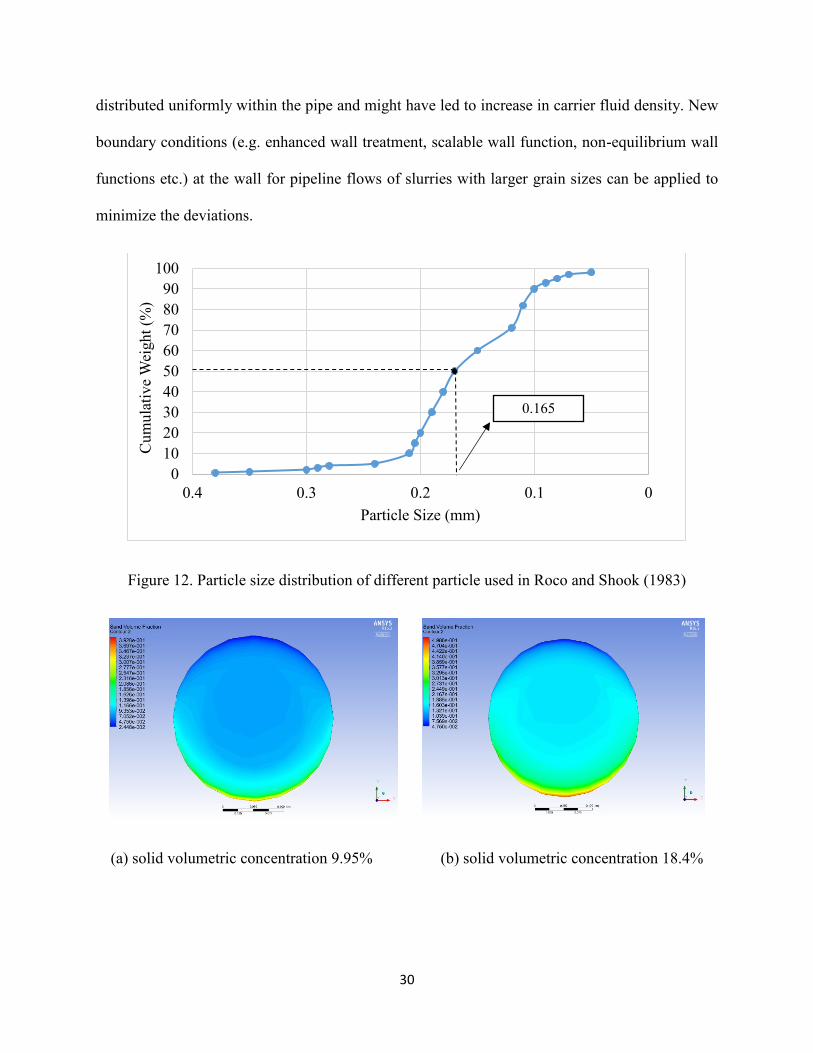
was 0.165 mm. Particle Size Distribution (PSD) from literature is shown in Figure 12 from where

0.165 mm is selected as mean size. Mixture velocity 3.5 m/s and four different solid volumetric

concentrations (Cv) 9.95%, 18.4%, 26.8% and 33.8% respectively were considered for analysis.

0

10

20

30

40

50

60

70

80

90

100

0 0.1 0.2 0.3 0.4 0.5 0.6

Cu

mu

lati

ve

Wei

gh

t (%

)

Particle Size (mm)

0.1250.44

27

The contours of local volumetric concentration distributions of solid particles in the vertical cross

section planes (data from Roco and Shook (1983)) are shown in Figure 13. The contours were

collected from the CFD simulation results. It is understandable by analyzing the contours that the

regions of highest solid concentrations are located near the wall in the lower half of pipe cross

section which is due to the downward gravitational force.

Figure 9. Comparison of simulated pressure gradient with experimental data from Skudarnov et

al. (2001), Kaushal et al. (2005) and Skudarnov et al. (2004) at different inlet slurry velocity [dm

= sand particle diameter, Cv = sand volumetric concentrations]

0

1000

2000

3000

4000

5000

6000

7000

8000

0 1 2 3 4 5 6

Pre

ssure

Gra

die

nt

(Pa/

m)

Slurry Velocity (m/s)

Data from Skudarnov et al., 2004 (0.023 m Diameter, dm = 140 µm and Cv = 15%)

Data from Kaushal et al., 2005 (0.0549 m Diameter dm = 125 µm, 440 µm and Cv =

40%)Data from Skudarnov et al., 2001 (0.0221 cm Diameter, dm = 30 µm and Cv = 20%)

CFD Results (Skudarnov et al., 2004)

CFD Results (Kaushal et al., 2005)

28

Figure 10. Comparison of simulated solid local volumetric concentration across vertical

centerline with Gillies and Shook, 1994 (263 mm pipe diameter, dm = 0.18 mm, slurry velocity

3.1 m/s) [dm = sand particle diameter, Cv = sand volumetric concentrations]

-1.5

-1

-0.5

0

0.5

1

1.5

0 0.2 0.4 0.6

Y/R

Volumetric Concentration of Solid Particles

CFD Results (Cv = 14%)



Data from Gillies and Shook,

1994 (Cv = 14%)


1994 (Cv = 29%)


1994 (Cv = 45%)

29

Figure 11. Comparison of simulated and measured solid local volumetric concentration across

vertical centerline with Roco and Shook, 1983 (53.2 mm pipe diameter, dm = 0.165 mm, slurry

velocity 3.5 m/s) [dm = sand particle diameter, Cv = sand volumetric concentrations]

Although simulated results are in good agreement with experimental values in general, it should

be noted that the deviations are noticeable near the wall in the lower half of the cross-section

(Figure 10). One of the possible reasons could be abrasive rounding of these generous size particles

by repeated passages during experiment. This resulted in significant quantities of fines which were

-1.5

-1

-0.5

0

0.5

1

1.5

0 0.2 0.4 0.6

Y/R

Sand Concentration

CFD Results (Cv = 9.95%)




Data from Roco and Shook,

1983 (Cv = 9.95%)


1983 (Cv = 18.4%)


1983 (Cv = 26.8%)


1983 (Cv = 33.8%)

30

distributed uniformly within the pipe and might have led to increase in carrier fluid density. New

boundary conditions (e.g. enhanced wall treatment, scalable wall function, non-equilibrium wall

functions etc.) at the wall for pipeline flows of slurries with larger grain sizes can be applied to

minimize the deviations.

Figure 12. Particle size distribution of different particle used in Roco and Shook (1983)

(a) solid volumetric concentration 9.95% (b) solid volumetric concentration 18.4%

0

10

20

30

40

50

60

70

80

90

100

00.10.20.30.4

Cum

ula

tive

Wei

ght

(%)

Particle Size (mm)

0.165

31

(c) solid volumetric concentration 26.8% (d) solid volumetric concentration 33.8%

Figure 13. Solid concentration distribution in the vertical cross section plane (data from Roco

and Shook, 1983 where 53.2 mm pipe diameter, dm = 0.165 mm, slurry velocity 3.5 m/s) [dm =

sand particle diameter, Cv = sand volumetric concentrations]

Two Phase (solid-liquid) flow through Annuli

Pressure gradient (Pa/m) profiles of water-sand slurry flows through vertical concentric annuli are

compared with Ozbelge and Beyaz (2001) experimental data in Figure 14. For the CFD simulation,

the liquid phase was considered as water (density 9982 kg/m3, viscosity 0.001003 kg/m-s) and

solid phase was taken as feldspar (symbol K2O.Al2O3.SiO2, mean particle diameter 0.23 mm, mean

density 2500 kg/m3, range of slurry volumetric concentration 0.8%–1.8%). Length, OD and ID of

the annulus were 5 m, 0.125 m, and 0.025 m, respectively. As the inlet boundary conditions,

average velocities were specified in the range of 0.0738–0.197 m/s. In compliance to the

experimental conditions, a smooth pipe of stainless steel (density 8030 kg/m3) was used for the

simulation. The pipe was assumed to be vertical, i.e., gravity effect was included and gravitational

acceleration was directed opposite to outlet. No slip boundary conditions for liquid and solid phase

were used at the walls. Figure 14 shows the comparison among simulated and measured two-phase

32

frictional pressure drops. Very similar to the previous analyses, the simulated results are in good

agreement with the experimental values with an average discrepancy of only 3%.

Figure 14. Comparison of simulated two-phase frictional pressure gradient at different mixture

velocity and volume concentration of slurry with Ozbelge and Beyaz, 2001 (0.125 m outer

diameter, 0.025 m inner diameter, dm = 0.23 mm) [dm = sand particle diameter, Cv = sand

volumetric concentrations]

Two Phase (gas-liquid) flow through Pipeline

Figure 15 and Figure 16 show the comparisons of liquid water velocity profiles in two phase air-

water flow through horizontal pipeline. Axial velocities of vertical and horizontal positions are

presented in Figure 15 and Figure 16, respectively. The data presented by Kocamustafaogullari

0

50

100

150

200

250

300

350

400

0 0.05 0.1 0.15 0.2 0.25

Pre

ssure

Gra

die

nt

(Pa/

m)

Mixture Velocity (m/s)

CFD Results (volume concentration 1.8% v/v)CFD Results (volume concentration 1.5% v/v)CFD Results (volume concentration 1.0% v/v)CFD Results (volume concentration 0.8% v/v)Experiment (volume concentration 1.8% v/v)Experiment (volume concentration 1.5% v/v)Experiment (volume concentration 1.0% v/v)Experiment (volume concentration 0.8% v/v)

33

and Wang (1991) were used for these comparisons. For the experiments, diameter of pipeline was

50.4 mm, pipe length was 9000 mm, water was the liquid phase (mean velocity: 5.1 m/s), air was

gaseous phase (mean velocity: 0.25 m/s, volume fraction: 0.043), bubble size was 2 mm,

temperature was 25°C, and pipe roughness was 0.1 mm.

Figure 15. Comparison of simulated axial liquid velocity at vertical position with experimental

data from Kocamustafaogullari and Wang, 1991 (50.4 mm pipe diameter, da = 2 mm, Ca = 4.3%,

va = 0.25 m/s, vs = 5.1 m/s) [da = air bubble diameter, Ca = air volumetric concentrations, va = air

velocity, vw = water velocity]

From the analysis, simulated local velocity profile is agreeing with experiment having considerable

errors. The velocity profile from experiment has slight degree of asymmetry where velocity in the

pipe top region is lower than pipe bottom region. Due to the presence of gas particles and

gravitational effect on gas, liquid concentration is lower at top region of pipe. This results in

decreasing mixture velocity at upper half of pipe (gas velocity 0.25 m/s and water velocity 5.1

m/s).

0

0.1

0.2

0.3

0.4

0.5

0.6

0.7

0.8

0.9

1

0 1 2 3 4 5 6 7

Ver

tica

l P

osi

tion (

y/D

)

Axial Liquid Velocity (m/s)

Simulation

Experiment

34

Figure 16. Comparison of simulated axial liquid velocity at horizontal position with experimental

data from Kocamustafaogullari and Wang, 1991 (50.4 mm pipe diameter, da = 2 mm, Ca = 4.3%,

va = 0.25 m/s, vs = 5.1 m/s) [da = air bubble diameter, Ca = air volumetric concentrations, va = air

velocity, vw = water velocity]

Three Phase (solid-liquid-gas) flow through Pipeline

The simulation results of pressure gradients for air-water-sand three phase flows through

horizontal pipelines are compared in Figure 17 and Figure 18 with the experimental data available

in Fukuda and Shoji (1986), Kago et al. (1986) and Gillies et al. (1997). In the experiments

conducted by Fukuda and Shoji (1986), length of pipe was 2.9 m, diameter of pipe was 0.0416 m,

water was the liquid phase (density 998.2 kg/m3, viscosity 0.001 kg/m-s), silica sand particle was

the solid phase (density 2650 kg/m3, mean particle diameter 0.074 mm) and air was the gaseous

phase (density 1.225 kg/m3, viscosity 1.789*10-5 kg/m-s). Mean particle diameter of sand particle

was selected from particle size distribution chart (Figure 19). Pipe wall material was Polycarbonate

(transparent, smooth pipe). Fukuda and Shoji (1986) used solid volume concentrations of 8.8%,

0

1

2

3

4

5

6

7

0 0.2 0.4 0.6 0.8 1

Ax

ial

Liq

uid

Vel

oci

ty (

m/s

)

Horizontal Position (x/D)

Experiment Simulation

35

13.3% and 24.7% in slurry and 3 m/s slurry velocity with different velocities of gas. For the

experiments reported in Kago et al. (1986), length of pipe was 5.95 m, diameter of pipe was 51.5

mm and the three phase fluid was comprised of water, air and sand (Silica Alumina catalyst particle

with density 1520 kg/m3, mean particle diameter 0.059 mm and 40% volumetric concentration in

slurry). Wall material was similar to the one used by Fukuda and Shoji (1986). Slurry velocity was

maintained at 0.5 m/s. In case of Gillies et al. (1997), length of pipe was 5 m, diameter of pipe was

Figure 17. Comparison of simulated pressure gradient as a function of gas velocity with

experimental data from Fukuda and Shoji, 1986 (0.0416 m pipe diameter, 0.074 mm sand

particle diameter, 2 mm air bubble diameter, 3 m/s slurry velocity) and Kago et al., 1986 (0.0515

m pipe diameter, 0.059mm sand particle diameter, 2 mm air bubble diameter, 0.5 m/s slurry

velocity)

0

1000

2000

3000

4000

5000

0 0.5 1 1.5 2 2.5 3

Pre

ssure

Dro

p (

Pa/

m)

Superficial Gas Velocity (m/s)





Data from Fukuda and Shoji, 1986 (Cv = 8.8%)



Data from Kago et al., 1986 (Cv = 40%)

36

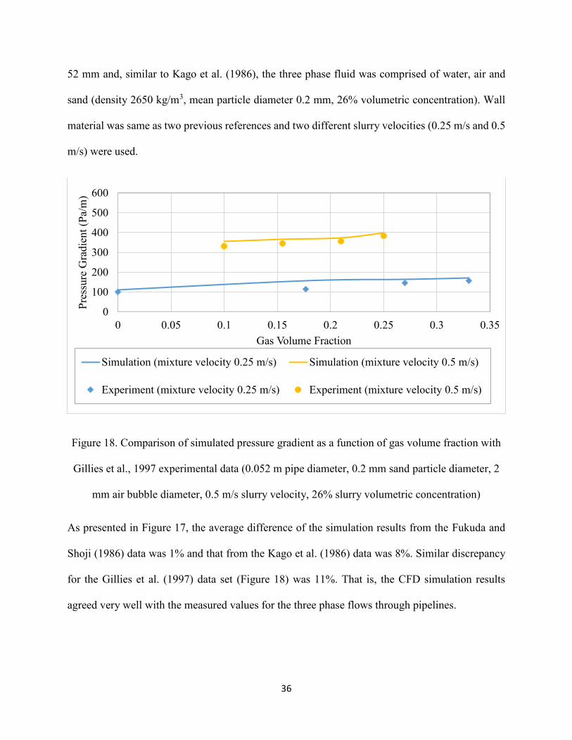
52 mm and, similar to Kago et al. (1986), the three phase fluid was comprised of water, air and

sand (density 2650 kg/m3, mean particle diameter 0.2 mm, 26% volumetric concentration). Wall

material was same as two previous references and two different slurry velocities (0.25 m/s and 0.5

m/s) were used.

Figure 18. Comparison of simulated pressure gradient as a function of gas volume fraction with

Gillies et al., 1997 experimental data (0.052 m pipe diameter, 0.2 mm sand particle diameter, 2

mm air bubble diameter, 0.5 m/s slurry velocity, 26% slurry volumetric concentration)

As presented in Figure 17, the average difference of the simulation results from the Fukuda and

Shoji (1986) data was 1% and that from the Kago et al. (1986) data was 8%. Similar discrepancy

for the Gillies et al. (1997) data set (Figure 18) was 11%. That is, the CFD simulation results

agreed very well with the measured values for the three phase flows through pipelines.

0

100

200

300

400

500

600

0 0.05 0.1 0.15 0.2 0.25 0.3 0.35

Pre

ssure

Gra

die

nt

(Pa/

m)

Gas Volume Fraction

Simulation (mixture velocity 0.25 m/s) Simulation (mixture velocity 0.5 m/s)

Experiment (mixture velocity 0.25 m/s) Experiment (mixture velocity 0.5 m/s)

37

Figure 19. Particle size distribution of different particle used in Fukuda and Shoji (1986)

Future Plan

Continuation of the current work is in progress. It is expected to lead to find out numerical

dependencies of different parameters by conducting parametric studies in details. Also, analyzing

solid concentration profile of slurry will help to find out the deposition velocity, i.e., the minimum

superficial velocity of mixture required to prevent accumulation of solids. Experimental facilities

have already been developed in Texas A&M University at Qatar (TAMUQ) to comprehensively

study the drilling and hole-cleaning process conditions. Applying the current CFD model to predict

various experimentally tested process conditions, the next step is to elaborately study the

parametric effects on the pressure losses and the concentration profiles of multiphase flows

through pipelines and annuli involving both Newtonian and non-Newtonian fluids. Apart from

this, another ongoing research is to analyze Fluid Structure Interaction (FSI). Due to multiphase

flows through pipelines and annuli under different conditions, pressure stresses are formed which

may deform the pipe/annulus. This study is expected to be significant for the process safety of

different multiphase flow systems.

0

10

20

30

40

50

60

70

80

90

100

00.020.040.060.080.10.120.140.16

Cum

ula

tive

Wei

ght

(%)

Particle Size (mm)

0.074

38

Conclusion

The current study helps to validate a CFD model of multiphase flow through pipeline and annuli.

The model can be applied to different applications, especially the ones related to oil and gas

industry. The analysis can give idea of selecting optimum range of particle size, volumetric

concentration of slurry and mixture velocity during operation using this model. It demonstrated an

acceptable agreement with experimental results from single phase to three phase flow, which

eventually validates the developed CFD model for further applications. The present investigation

can be summarized as follows:

• On the basis of related literatures and experimental validations, the Eulerian model as the

multiphase model and the Reynolds stress model (RSM) as the turbulence model were

selected as the optimum models in this study.

• Mesh size and inflation layers near the wall were finalized after proper checking of the mesh

independency of the simulation results and in consideration of the convergence requirement

of the dimensionless wall distance (y+ > 30). The minimum numbers of nodes for the pipeline

and annular geometries were 135000 and 540000, respectively. Furthermore, 10 inflation

layers with a growth rate of 20% were used near the boundaries.

• Length-independent results were ensured through analysis of the output parameter, i.e.,

pressure gradient at different cross-sections of the pipeline and annuli (Figure 3). This was

done to verify the minimum flow development section or entrance length (50Dh) and to

analyze the variation of pressure gradients along the length.

• Good agreement of the simulation results with the corresponding experimental values were

found over a wide range of properties and flow conditions (Table 1). Considering pressure

gradient results from all cases, the average difference was less than 15% with a maximum

39

value of 30% (Figure 20). Also, velocity profile and sand concentration profile along cross

section provided a reasonable discrepancy (< 15%). These indicate the validity of our model

within the given range of process conditions which is wide enough to cover different types of

operating conditions at several industries.

• Future works are underway to ensure that the present CFD model is applicable to the

simulation of industrially important multiphase flow conditions. The following industries are

expected to benefit from the use of this model: chemical process plants, petroleum industries,

food processing industries, and nuclear plants. Further analysis is required to select the values

of different coefficients and constants, such as the coefficient of lift, coefficient of drag,

restitution coefficient, and wall boundary conditions, to minimize errors and widen the

application range of this model.

Figure 20. Overall simulation predictions of different experiment data

0

1000

2000

3000

4000

5000

6000

7000

0 2000 4000 6000

Sim

ula

tion P

redic

tion (

Pa/

m)

Experiment (Pa/m)

Kelessidis et al., 2011

Camçi, 2003

Kaushal et al., 2005 (single

phase)Skudarnov et al., 2004 (single

phase)Skudarnov et al., 2004 (two

phase)Kaushal et al., 2005 (two phase)

Skudarnov et al., 2001

Ozbelge and Beyaz (2001)

Fukuda and Shoji (1986)

Gillies et al. (1997)

Kago et al. (1986)

40

Acknowledgments

The authors are thankful to Faculty of Engineering and Applied Science of Memorial University,

Texas A&M University at Qatar and ANSYS Inc. (License Server Machine:

lmserver2.engr.mun.ca) for helping this project.

Reference

Alder, B. J., and T. E. Wainwright. "Studies in molecular dynamics. II. Behavior of a small number

of elastic spheres." The Journal of Chemical Physics 33, no. 5 (1960): 1439-1451.

Anderson, T. Bo, and Roy Jackson. "Fluid mechanical description of fluidized beds. Equations of

motion." Industrial & Engineering Chemistry Fundamentals 6, no. 4 (1967): 527-539.

Aude, T. C., T. L. Thompson, and E. J. Wasp. "Economics of slurry pipeline systems." Publication

of: Cross (Richard B) Company 15, no. Proc Paper (1974).

Aude, T. C., T. L. Thompson, and E. J. Wasp. "Slurry-pipeline systems for coal; other solids come

of age." Oil Gas J.;(United States) 73, no. 29 (1975).

Baltussen, M. W., L. J. H. Seelen, J. A. M. Kuipers, and N. G. Deen. "Direct Numerical

Simulations of gas–liquid–solid three phase flows." Chemical Engineering Science 100

(2013): 293-299.

Bello, Oladele O., Kurt M. Reinicke, and Catalin Teodoriu. "Particle Holdup Profiles in Horizontal

Gas‐liquid‐solid Multiphase Flow Pipeline." Chemical engineering & technology 28, no. 12

(2005): 1546-1553.

Bowen, R. M. "Theory of Mixtures in Continuum Physics, Vol. Ill, Eringen, A. C, ed." (1976).

Camçı, Gülden. "Application of isokinetic sampling technique for local solid densities in upward

liquid-solid flows through an annulus." PhD diss., METU, 2003.

41

Camçi, Gülden, and Tülay A. Özbelge. "Determination of dilute slurry densities in a vertical

annulus using isokinetic sampling." Chem. Eng. Comm.193, no. 11 (2006): 1482-1501.

Chapman, Sydney, and Thomas George Cowling. The mathematical theory of non-uniform gases:

an account of the kinetic theory of viscosity, thermal conduction and diffusion in gases.

Cambridge university press, 1970.

Chen, Ning Hsing. "An explicit equation for friction factor in pipe." Industrial & Engineering

Chemistry Fundamentals 18, no. 3 (1979): 296-297.

Chen, Liangyong, Yufeng Duan, Wenhao Pu, and Changsui Zhao. "CFD simulation of coal-water

slurry flowing in horizontal pipelines." Korean journal of chemical engineering 26, no. 4

(2009): 1144-1154.

Cornelissen, Jack T., Fariborz Taghipour, Renaud Escudié, Naoko Ellis, and John R. Grace. "CFD

modelling of a liquid–solid fluidized bed." Chemical Engineering Science 62, no. 22 (2007):

6334-6348.

Dewangan, Satish K., and Shobha L. Sinha. "Exploring the hole cleaning parameters of horizontal

wellbore using two-phase Eulerian CFD approach." The Journal of Computational Multiphase

Flows 8, no. 1 (2016): 15-39.

Durand, Robert. "Transport hydraulique de graviers et galets en conduite." La Houille

Blanche (1951): 609-619.

Durand, R., and E. Condolios. "The hydraulic transportation of coal and solid material in pipes."

In Processing of Colloquium on Hransport of Coal, National Coal Board, Nov, vol. 5. 1952.

Eraslan, Ahmet N., and Tülay A. Özbelge. "Assessment of flow and heat transfer characteristics

for proposed solid density distributions in dilute laminar slurry upflows through a concentric

annulus." Chemical engineering science 58, no. 17 (2003): 4055-4069.

42

Escudier, M. P. P. J., P. J. Oliveira, F. Pinho, and S. Smith. "Fully developed laminar flow of non-

Newtonian liquids through annuli: comparison of numerical calculations with

experiments." Experiments in fluids 33, no. 1 (2002): 101-111.

Fluent, A. N. S. Y. S. "12.0/12.1 Documentation." Users Guide Manual, Ansys Inc (2009).

Fu, S., B. E. Launder, and M. A. Leschziner. "Modelling strongly swirling recirculating jet flow

with Reynolds-stress transport closures." In 6th Symposium on Turbulent Shear Flows, pp. 17-

6. 1987.

Fukuda, Tadashi, and Yasuo Shoji. "Pressure Drop and Heat Transfer for Tree Phase Flow: 1st

Report, Flow in Horizontal Pipes." Bulletin of JSME 29, no. 256 (1986): 3421-3426.

Gibson, M. M., and B. E. Launder. "Ground effects on pressure fluctuations in the atmospheric

boundary layer." Journal of Fluid Mechanics 86, no. 3 (1978): 491-511.

Gillies, R. G., M. J. McKibben, and C. A. Shook. "Pipeline flow of gas, liquid and sand mixtures

at low velocities." Journal of Canadian Petroleum Technology 36, no. 09 (1997).

Gillies, R. G., and C. A. Shook. "Concentration distributions of sand slurries in horizontal pipe

flow." Particulate science and technology 12, no. 1 (1994): 45-69.

Gopaliya, Manoj Kumar, and D. R. Kaushal. "Analysis of effect of grain size on various

parameters of slurry flow through pipeline using CFD." Particulate Science and

Technology 33, no. 4 (2015): 369-384.

Govier, George Wheeler, and Khalid Aziz. The flow of complex mixtures in pipes. Vol. 469. New

York: Van Nostrand Reinhold, 1972.

Haaland, Skjalg E. "Simple and explicit formulas for the friction factor in turbulent pipe

flow." Journal of Fluids Engineering 105, no. 1 (1983): 89-90.

43

Hatate, Yasuo, Hiroshi Nomura, Takanori Fujita, Shuichi Tajiri, and Atsushi Ikari. "Gas holdup

and pressure drop in three-phase horizontal flows of gas-liquid-fine solid particles

system." Journal of chemical engineering of Japan 19, no. 4 (1986): 330-335.

Hernández, Franz H., Armando J. Blanco, and Luis Rojas-Solórzano. "CFD modeling of slurry

flows in horizontal pipes." In ASME 2008 Fluids Engineering Division Summer Meeting

collocated with the Heat Transfer, Energy Sustainability, and 3rd Energy Nanotechnology

Conferences, pp. 857-863. American Society of Mechanical Engineers, 2008.

Kago, Tokihiro, Tetsuya Saruwatari, Makoto Kashima, Shigeharu Morooka, and Yasuo Kato.

"Heat transfer in horizontal plug and slug flow for gas-liquid and gas-slurry systems." Journal

of chemical engineering of Japan 19, no. 2 (1986): 125-131.

Kaushal, D. R., A. Kumar, Yuji Tomita, Shigeru Kuchii, and Hiroshi Tsukamoto. "Flow of mono-

dispersed particles through horizontal bend." International Journal of Multiphase Flow 52

(2013): 71-91.

Kaushal, D. R., Kimihiko Sato, Takeshi Toyota, Katsuya Funatsu, and Yuji Tomita. "Effect of

particle size distribution on pressure drop and concentration profile in pipeline flow of highly

concentrated slurry." International Journal of Multiphase Flow 31, no. 7 (2005): 809-823.

Kelessidis, V. C., G. E. Bandelis, and J. Li. "Flow of dilute solid-liquid mixtures in horizontal

concentric and eccentric annuli." Journal of Canadian Petroleum Technology 46, no. 05

(2007).

Kelessidis, Vassilios C., Panagiotis Dalamarinis, and Roberto Maglione. "Experimental study and

predictions of pressure losses of fluids modeled as Herschel–Bulkley in concentric and

eccentric annuli in laminar, transitional and turbulent flows." Journal of Petroleum Science

and Engineering 77, no. 3 (2011): 305-312.

44

Kocamustafaogullari, G., and Z. Wang. "An experimental study on local interfacial parameters in

a horizontal bubbly two-phase flow." International journal of multiphase flow 17, no. 5 (1991):

553-572.

Krieger, Irvin M. "Rheology of monodisperse latices." Advances in Colloid and Interface

Science 3, no. 2 (1972): 111-136.

Kumar Gopaliya, Manoj, and D. R. Kaushal. "Modeling of sand-water slurry flow through

horizontal pipe using CFD." Journal of Hydrology and Hydromechanics 64, no. 3 (2016): 261-

272.

Lahiri, S. K., and K. C. Ghanta. "Computational technique to predict the velocity and concentration

profile for solid-liquid slurry flow in pipelines." In 17th International Conference on

Hydrotransport, pp. 149-175. 2007.

Launder, B. E., G. Jr Reece, and W. Rodi. "Progress in the development of a Reynolds-stress

turbulence closure." Journal of fluid mechanics 68, no. 3 (1975): 537-566.

Li, Li, Hai-liang Xu, and Fang-qiong Yang. "Three-phase flow of submarine gas hydrate pipe

transport." Journal of Central South University 22, no. 9 (2015): 3650-3656.

Lien, Fue-Sang, and M. A. Leschziner. "Assessment of turbulence-transport models including non-

linear RNG eddy-viscosity formulation and second-moment closure for flow over a backward-

facing step." Computers & Fluids23, no. 8 (1994): 983-1004.

Lin, C. X., and M. A. Ebadian. "A numerical study of developing slurry flow in the entrance region

of a horizontal pipe." Computers & Fluids 37, no. 8 (2008): 965-974.

Ling, J., P. V. Skudarnov, C. X. Lin, and M. A. Ebadian. "Numerical investigations of liquid–solid

slurry flows in a fully developed turbulent flow region." International Journal of Heat and

Fluid Flow 24, no. 3 (2003): 389-398.

45

Liu, Xiaoxing, Yuki Aramaki, Liancheng Guo, and Koji Morita. "Numerical simulation of gas–

liquid–solid three-phase flow using particle methods." Journal of Nuclear Science and

Technology 52, no. 12 (2015): 1480-1489.

Markatos, N. C. "The mathematical modelling of turbulent flows." Applied Mathematical

Modelling 10, no. 3 (1986): 190-220.

Newitt, D. D. "Hydraulic conveying of solids in horizontal pipes." Trans. Inst. Chem. Engrs. 33

(1955): 93-103.

Nourmohammadi, Khosrow, P. K. Hopke, and J. J. Stukel. "Turbulent air flow over rough surfaces.

II. Turbulent flow parameters." ASME, Transactions, Journal of Fluids Engineering 107

(1985): 55-60.

O'Brien, Morrough P. "Review of the theory of turbulent flow and its relation to sediment‐

transportation." Eos, Transactions American Geophysical Union 14, no. 1 (1933): 487-491.

Orell, Aluf. "The effect of gas injection on the hydraulic transport of slurries in horizontal

pipes." Chemical Engineering Science 62, no. 23 (2007): 6659-6676.

Özbelge, T. A., and A. Beyaz. "Dilute solid–liquid upward flows through a vertical annulus in a

closed loop system." International journal of multiphase flow 27, no. 4 (2001): 737-752.

Özbelge, Tülay A., and Ahmet N. Eraslan. "A computational hydrodynamic and heat transfer study

in turbulent up-flows of dilute slurries through a concentric annulus." Turkish Journal of

Engineering and Environmental Sciences 30, no. 1 (2006): 1-13.

Özbelge, Tülay A., and Sema H. Köker. "Heat transfer enhancement in water—feldspar upflows

through vertical annuli." International journal of heat and mass transfer 39, no. 1 (1996): 135-

147.

46

Özbelge, Tülay A., and Gülden Camçi Ünal. "A new correlation for two-phase pressure drops in

fully developed dilute slurry up-flows through an annulus." Chemical Engineering

Communications 196, no. 4 (2008): 491-498.

Page, Chester H. "The International System of Units [SI]." The Physics Teacher 9, no. 7 (1971):

379-381.

Pouranfard, A. R., D. Mowla, and F. Esmaeilzadeh. "An experimental study of drag reduction by

nanofluids in slug two-phase flow of air and water through horizontal pipes." Chinese Journal

of Chemical Engineering 23, no. 3 (2015): 471-475.

Rahman, M. A., K. Freeman Adane, and R. Sean Sanders. "An improved method for applying the

lockhart–martinelli correlation to three‐phase gas–liquid–solid horizontal pipeline flows." The

Canadian Journal of Chemical Engineering 91, no. 8 (2013): 1372-1382.

Roco, M. C., and C. A. Shook. "Modeling of slurry flow: the effect of particle size." The Canadian

Journal of Chemical Engineering 61, no. 4 (1983): 494-503.

Roco, M. C., and C. A. Shook. "Computational method for coal slurry pipelines with

heterogeneous size distribution." Powder Technology 39, no. 2 (1984): 159-176.

Rouse, Hunter. "Modern conceptions of the mechanics of turbulence." Trans. ASCE 102 (1937):

463-543.

Rushd, Sayeed, Sultan, Rasel A., Kelessidis, Vassilios C., and Rahman, M. A. "Investigation of

Pressure Losses in Eccentric Inclined Annuli." In 36th International Conference on Ocean,

Offshore & Arctic Engineering. American Society of Mechanical Engineering, 2017.

Sanders, R. Sean, Jason Schaan, and Melissa M. McKibben. "Oil sand slurry conditioning tests in

a 100 mm pipeline loop." The Canadian Journal of Chemical Engineering 85, no. 5 (2007):

756-764.

47

Scott, D. S., and P. K. Rao. "Transport of solids by gas‐liquid mixtures in horizontal pipes." The

Canadian Journal of Chemical Engineering 49, no. 3 (1971): 302-309.

Seshadri, V. "Basic process design for a slurry pipeline." Proc. The Short Term Course on Design

of pipelines for transporting liquid and solid materials, IIT, Delhi (1982).

Seshadri, V. "Concentration and size distribution of solids in a slurry pipeline." In Proc. 11th Nat.

Conference on Fluid Mechanics and Fluid Power, BHEL, Hyderabad, 1982. 1982.

Silva, Moises A., and Subhash N. Shah. "Friction pressure correlations of Newtonian and non-

Newtonian fluids through concentric and eccentric annuli." In SPE/ICoTA Coiled Tubing

Roundtable. Society of Petroleum Engineers, 2000.

Skudarnov, P. V., H. J. Kang, C. X. Lin, M. A. Ebadian, P. W. Gibbons, F. F. Erian, and M. Rinker.

"Experimental investigation of single-and double-species slurry transportation in a horizontal

pipeline." In Proc. ANS 9th International Topical Meeting on Robotics and Remote Systems,

Seattle, WA. 2001.

Skudarnov, P. V., C. X. Lin, and M. A. Ebadian. "Double-species slurry flow in a horizontal

pipeline." Journal of fluids engineering 126, no. 1 (2004): 125-132.

Syamlal, Madhava, William Rogers, and Thomas J. O’Brien. "MFIX documentation: Theory

guide." National Energy Technology Laboratory, Department of Energy, Technical Note

DOE/METC-95/1013 and NTIS/DE95000031 (1993).

Thomas, David G. "Transport characteristics of suspension: VIII. A note on the viscosity of

Newtonian suspensions of uniform spherical particles." Journal of Colloid Science 20, no. 3

(1965): 267-277.

Toda, M., K. Shimazaki, and S. Maeda. "Pressure drop of three-phase flow in horizontal

pipes." Kagaku Kogaku Ronbunshu 4 (1978): 56-62.

48

Van Sint Annaland, M., N. G. Deen, and J. A. M. Kuipers. "Numerical simulation of gas–liquid–

solid flows using a combined front tracking and discrete particle method." Chemical

engineering science 60, no. 22 (2005): 6188-6198.

Vasquez, Sergio. "A Phase Coupled Method for Solving Multiphase Problems on Unstructured

Mesh." In ASME Fluids Engineering Division Summer Meeting. 2000.

Vijiapurapu, Sowjanya, and Jie Cui. "Performance of turbulence models for flows through rough

pipes." Applied Mathematical Modelling 34, no. 6 (2010): 1458-1466.

Vocadlo, J. J., and M. E. Charles. "Transportation of slurries." Canadian Mining and Metallurgical

Bulletin 65, no. 726 (1972).

Wakeman, T., and W. Tabakoff. "Measured particle rebound characteristics useful for erosion

prediction." In ASME 1982 International Gas Turbine Conference and Exhibit, pp.

V003T05A005-V003T05A005. American Society of Mechanical Engineers, 1982.

Washino, K., H. S. Tan, A. D. Salman, and M. J. Hounslow. "Direct numerical simulation of solid–

liquid–gas three-phase flow: Fluid–solid interaction." Powder technology 206, no. 1 (2011):

161-169.

Wasp, Edward J., John P. Kenny, and Ramesh L. Gandhi. "Solid--liquid flow: slurry pipeline

transportation. [Pumps, valves, mechanical equipment, economics]." Ser. Bulk Mater. Handl.;

(United States) 1, no. 4 (1977).

Lin, C. X. "Double-Species Slurry Flow in a Horizontal Pipeline." (2004).

Zagarola, M. V., and A. J. Smits. "Scaling of the mean velocity profile for turbulent pipe flow."

Physical review letters 78, no. 2 (1997): 239.

49

Chapter 2. Pressure Losses and Settling Conditions in a Horizontal Annulus

Rasel A Sultan1, M. A. Rahman2, Sayeed Rushd2, Sohrab Zendehboudi1, Vassilios C. Kelessidis3

1Faculty of Engineering and Applied Science, Memorial University of Newfoundland, Canada

2Texas A&M University at Qatar, Doha, Qatar

3Petroleum Institute, Abu Dhabi, UAE

Abstract

Estimation of pressure losses and settling conditions are vital in the hydraulic design of annular

drill holes in Petroleum Industry. The present study investigates the effects of fluid velocity, fluid

type, particle size, particle concentration, drill pipe rotation speed and drill pipe eccentricity on

pressure losses and settling conditions using computational fluid dynamics (CFD). The

eccentricity of the drill pipe is varied in the range of 0 – 50% and it rotates about its own axis at 0

– 150 rpm. The diameter ratio of the simulated drill hole is 0.56. This study is about the numerical

simulation of turbulent conditions. Experimental data confirmed the validity of current CFD model

developed using ANSYS 16.2 platform. The goal of the current work is to develop a

comprehensive CFD tool that can be used for modeling the hydraulic conditions associated with

hole cleaning in extended reach drilling.

Introduction

In the petroleum industry, predicting frictional pressure losses and settling conditions for the

transportation of drilling fluids in the annuli are important for drilling operations. Inaccurate

predictions can lead to a number of costly drilling problems. A few examples of such problems

are loss of circulation, kicks, blockage, wear, abrasion, and improper rig power selection. The

existing empirical models become less accurate as those involve many simplified assumptions.

CFD simulations help to minimize such assumptions by using the physics based Navier Stokes

50

equations to model the hydrodynamics of the flow system. Current work is focused on developing

a comprehensive CFD model which is capable of considering the effects of all important drilling

parameters, such as fluid velocity, fluid type, particle size, particle concentration, drill pipe rotation

speed and drill pipe eccentricity.

Literature Review

The estimation of pressure loss in an annulus is more difficult compared to pipe flow due to the

complexities in hydraulics resulting from the complex geometry [1, 2]. From an empirical

perspective, the issue is usually addressed by replacing pipe diameter in the pipe flow models with

an “effective diameter” of annulus. A number of definitions of “effective diameter” have been

proposed till date. However, it is difficult to select a definition for a field application as those were

developed and/or applied empirically. A comparison of multiple definitions in predicting pressure

losses is presented by Anifowoshe and Osisanya [3]. Other issues that make the estimation of

pressure losses in drilling holes difficult are the eccentricity and the rotational speed of inner drill

pipe. Many studies have been done on the flow of non-Newtonian fluids in annuli to introduce

empirical/analytical models which allow to take these effects into account [1, 3-10]. The results of

the previous studies show that the annular pressure losses for non-Newtonian (power law) fluids

flowing in a drill hole depend on drill pipe rotation speed, fluid properties, flow regimes

(laminar/transitional/turbulent), diameter ratio, eccentricity and equivalent hydrodynamic

roughness.

Using commercially available CFD packages like ANSYS FLUENT to predict pressure losses for

the annular transportation of drilling fluids is comparatively a new approach. Sorgun and

Ozbayoglu [9] demonstrated the better performance of CFD model compared to the existing

empirical models in predicting frictional pressure losses. Sorgun [8] investigated the effect of pipe

51

eccentricity on pressure loss, tangential velocity, axial velocity and effective viscosity by using

CFD. Erge et al. [6] presented a CFD modeling approach which is applicable to estimate frictional

pressure losses in an eccentric annulus with inner pipe rotation while circulating yield power law

fluids. However, most of these CFD studies were limited to the laminar flow of a single phase in

hydro dynamically smooth annuli.

Annular flow of drilling fluids containing cuttings, i.e., slurry has not been studied in sufficient

details. Examples of works in the field of annular slurry flow are [11-14]. Focus of these studies

were to understand the hydrodynamics of the slurry flow in annulus from real time experiments

and to produce empirical models based on data analysis. Recently, different researchers [15-17]

have used CFD in studying the transportation of slurry in annuli. Ofei [15] examined the effect of

the rheological parameters of the carrying fluids on the velocity of solid. Sorgun and Ulker [16]

compared the predictions of pressure losses obtained using Artificial Neural Network (ANN) and

CFD. Both methods produced comparable results. Sun et al. [17] studied the effects of inclination,

rotational speed and flow rate on the distribution of solid concentration and the frictional pressure

loss. Similar to the single phase annular flow works, most of these CFD studies were limited to

the laminar slurry flow conditions.

Methods

CFD Simulation

In the current work, the CFD simulation model of the annular slurry flow is developed using

ANSYS Fluent 16.2 platform. Following previous works [18-20], a multi-fluid granular model is

used to describe the flow behavior of a fluid-solid mixture. The granular version of Eulerian model

is selected as the multiphase model. This is because high solid volume fraction is expected to be

used for this study and the granular version captures the hydrodynamics of high concentration

52

slurries consisting of varying grain sizes. It allows modeling of multiple separate but interacting

phases. The phases can be liquids, gases, or solids in nearly any combination. The Eulerian

treatment is used for each phase, in contrast to the Eulerian-Lagrangian treatment that is used for

the discrete phase model.

The description of multiphase flow as interpenetrating continua incorporates the concept of phasic

volume fractions, which represent the space occupied by each phase. Each phase satisfies the laws

of conservation of mass and momentum individually. The conservation equations are modified by

averaging the local instantaneous balance for each of the phases [21] or by using the mixture theory

approach [22]. A detailed description is available in Appendix A.

For Eulerian multiphase calculations, the phase coupled SIMPLE (PC-SIMPLE) algorithm is used

for the pressure-velocity coupling. PC-SIMPLE is an extension of the SIMPLE algorithm to

multiphase flows [23, 24]. The velocities coupled by phases are solved in a segregated fashion.

The block algebraic multigrid scheme used by the density-based solver is used to solve a vector

equation formed by the velocity components of all phases simultaneously [25]. Then, a pressure

correction equation is built based on total volume continuity. Pressure and velocities are then

corrected so as to satisfy the continuity constraints.

To ensure stability and convergence of iterative process, a second order upwind discretization was

used for momentum equation and first upwind discretization was employed for volume fraction,

turbulent kinetic energy and its dissipation. Upwinding refers to the face value derived from

quantities in the cell upstream, or "upwind,'' relative to the direction of the normal velocity. When

first-order accuracy is desired, quantities at cell faces are determined by assuming that the cell-

center values of any field variable represent a cell-average value and hold throughout the entire

cell; the face quantities are identical to the cell quantities. Thus, the face value is set equal to the

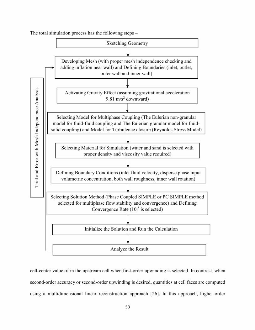
53

The total simulation process has the following steps –

cell-center value of in the upstream cell when first-order upwinding is selected. In contrast, when

second-order accuracy or second-order upwinding is desired, quantities at cell faces are computed

using a multidimensional linear reconstruction approach [26]. In this approach, higher-order

Sketching Geometry

Developing Mesh (with proper mesh independence checking and

adding inflation near wall) and Defining Boundaries (inlet, outlet,

outer wall and inner wall)

Activating Gravity Effect (assuming gravitational acceleration

9.81 m/s2 downward)

Selecting Model for Multiphase Coupling (The Eulerian non-granular

model for fluid-fluid coupling and The Eulerian granular model for fluid-

solid coupling) and Model for Turbulence closure (Reynolds Stress Model)

Selecting Material for Simulation (water and sand is selected with

proper density and viscosity value required)

Defining Boundary Conditions (inlet fluid velocity, disperse phase input

volumetric concentration, both wall roughness, inner wall rotation)

Selecting Solution Method (Phase Coupled SIMPLE or PC SIMPLE method

selected for multiphase flow stability and convergence) and Defining

Convergence Rate (10-5 is selected)

Initialize the Solution and Run the Calculation

Tri

al a

nd E

rro

r w

ith M

esh I

ndep

enden

ce A

nal

ysi

s

Analyze the Result

54

accuracy is achieved at cell faces through a Taylor series expansion of the cell-centered solution

about the cell centroid.

Turbulence Model Selection

Turbulent quantities for fluid flow are computed using Reynolds Stress Model [27-29].

Abandoning the isotropic eddy-viscosity hypothesis, the RSM closes the Reynolds-averaged

Navier-Stokes equations by solving transport equations for the Reynolds stresses, together with an

equation for the dissipation rate [30]. Here five additional transport equations are required in 2D

flows and seven additional transport equations must be solved in 3D (please see Appendix B for

further details). The turbulence model was selected for the current work analyzing the relative

performance of different models. A typical example of the analysis is presented in Figure 1. In this

figure, % Difference refers to the percentile difference between the experimental measurements of

pressure loss and the corresponding CFD predictions. In most cases, the difference was less than

10% when RSM was used. A list of the important results is presented in Table 1.

Figure 1. Performance of turbulence models in predicting pressure loss (Data Source: Kaushal et

al., 2005 [40])

0

10

20

RSM SST K-Omega Standard K-Omega

% D

iffe

ren

ce

55

Table 1. Analysis of Turbulence Model Performance

Reference Experimental Conditions % Difference

[100(Experiment – Simulation)/Experiment]

RSM SST

k-ω

Standard

k-ω

Standard

k-ε

Kaushal et

al. (2005)

[40]

Pipe orientation: Horizontal

Pipe dia.: 0.0549 m

Pipe material of construction:

Stainless Steel (density 8030

kg/m3, smooth wall)

Fluid: Single phase water

(density: 998.2 Kg/m3, viscosity:

0.001003 Kg/m-s)

Fluid velocity: 2 m/s

8 15 17 17.48

Camçi

(2003) [41]

Annulus orientation: Horizontal

and concentric

Annulus dimensions: 0.0432 m

ID, 0.123 m OD

9 17 20 23

56

Material of construction:

Aluminum (smooth wall)


Fluid velocity: 0.2 m/s

Kelessidis

et al.

(2011) [33]

Annulus orientation: Horizontal

and concentric

Annulus dimensions: 0.04 m ID,

0.07 m OD


Plexiglas (smooth wall)



8 13 16 22.2

Skudarnov

et al.

(2004) [42]

Pipe orientation: Horizontal

Pipe diameter: 0.023 m

Pipe material of construction:

Stainless Steel (Wall roughness:

32 µm)

-2 -2.8 -3 -3.2

57

Fluid: Two phase solid – liquid

slurry

Liquid: Water (density: 998.2

Kg/m3, viscosity: 0.001003

Kg/m-s)

Solid: Glass spheres (double-

species with densities of 2490

kg/m3 and 4200 kg/m3, 50% by

50% volume mixture, particle

diameter (dm): 140 µm,

volumetric concentration (Cv):

15%)


Ozbelge

and Beyaz

(2001) [35]

Annulus orientation: Vertical

and concentric


OD, 0.025 m ID



kg/m3, smooth wall)

-6 14 15 -15.1

58


slurry

Liquid: Water (density 998.2

Kg/m3, viscosity 0.001003

Kg/m-s)

Solid: Feldspar (mean particle

diameter 0.23 mm, mean density

2500 kg/m3, volumetric

concentration, Cv = 1.80%)


Ozbelge

and Beyaz

(2001) [35]

Annulus orientation: Vertical

and concentric


OD, 0.025 m ID



kg/m3, smooth wall)


slurry

-4 8 13 16

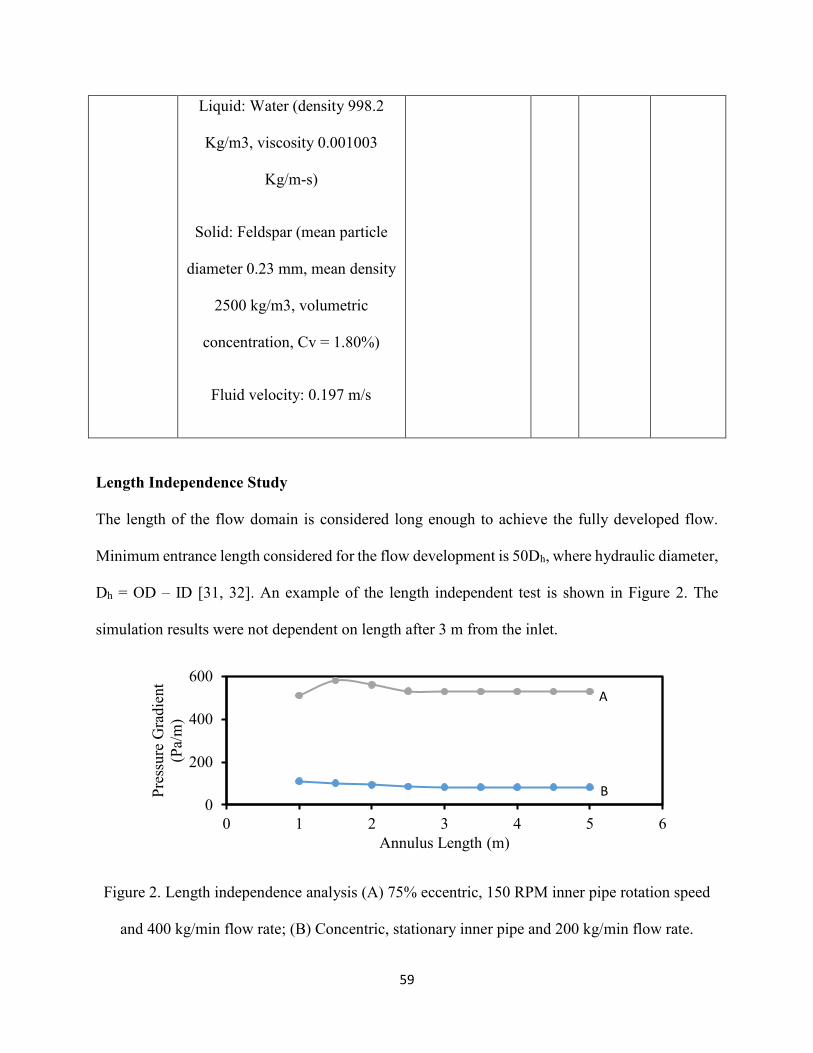
59

Liquid: Water (density 998.2

Kg/m3, viscosity 0.001003

Kg/m-s)

Solid: Feldspar (mean particle

diameter 0.23 mm, mean density

2500 kg/m3, volumetric

concentration, Cv = 1.80%)


Length Independence Study

The length of the flow domain is considered long enough to achieve the fully developed flow.

Minimum entrance length considered for the flow development is 50Dh, where hydraulic diameter,

Dh = OD – ID [31, 32]. An example of the length independent test is shown in Figure 2. The

simulation results were not dependent on length after 3 m from the inlet.

Figure 2. Length independence analysis (A) 75% eccentric, 150 RPM inner pipe rotation speed

and 400 kg/min flow rate; (B) Concentric, stationary inner pipe and 200 kg/min flow rate.

0

200

400

600

0 1 2 3 4 5 6

Pre

ssure

Gra

die

nt

(Pa/

m)

Annulus Length (m)

A

B

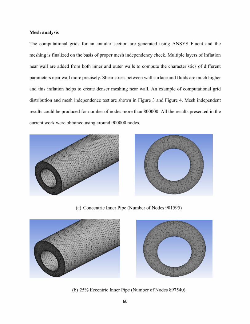
60

Mesh analysis

The computational grids for an annular section are generated using ANSYS Fluent and the

meshing is finalized on the basis of proper mesh independency check. Multiple layers of Inflation

near wall are added from both inner and outer walls to compute the characteristics of different

parameters near wall more precisely. Shear stress between wall surface and fluids are much higher

and this inflation helps to create denser meshing near wall. An example of computational grid

distribution and mesh independence test are shown in Figure 3 and Figure 4. Mesh independent

results could be produced for number of nodes more than 800000. All the results presented in the

current work were obtained using around 900000 nodes.

(a) Concentric Inner Pipe (Number of Nodes 901595)

(b) 25% Eccentric Inner Pipe (Number of Nodes 897540)

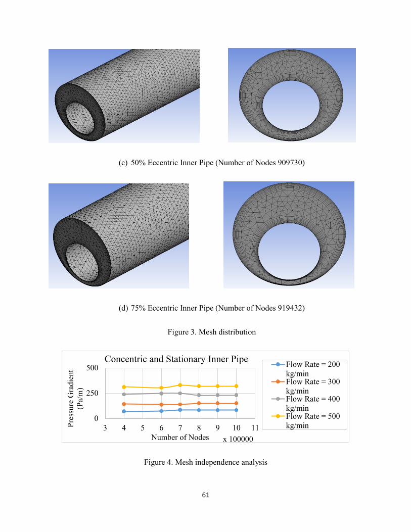
61

(c) 50% Eccentric Inner Pipe (Number of Nodes 909730)

(d) 75% Eccentric Inner Pipe (Number of Nodes 919432)

Figure 3. Mesh distribution

Figure 4. Mesh independence analysis

0

250

500

3 4 5 6 7 8 9 10 11Pre

ssure

Gra

die

nt

(Pa/

m)

Number of Nodes x 100000

Concentric and Stationary Inner PipeFlow Rate = 200

kg/minFlow Rate = 300



kg/min

62

Convergence rate analysis:

An optimum convergence rate of 10-5 was selected for the termination of iteration. Figure 5 shows

an example of the analysis used to find out optimum convergence rate within 10-6 – 10-4. The

simulation results varied when the convergence value was greater than 10-5. However, the results

did not change at all for the values less than 10-5.

Figure 5. An example of optimum convergence rate analysis

CFD Model Validation

As the preliminary step, the CFD modeling approach is validated with respect to the data available

in open literature. Few examples of the validation are presented as follows –

Single Phase Flow through Annuli

Sets of experimental data from Kelessidis et al. (2011) [33] and Camçi (2003) [41] are compared

in Figure 6 with the proposed CFD model. The geometry is taken from Kelessidis et al. (2011)

where inner diameter (ID) 0.04 m, outer diameter (OD) 0.07 m and length 5 m (horizontal

concentric annuli). Fluid is taken as water and wall material is Plexiglas (hydro dynamically

0

50

100

150

200

250

300

350

1.00E-06 1.00E-05 1.00E-04

Pre

ssure

Gra

die

nt

(Pa/

m)

Convergent Rate

Flow Rate = 200 kg/min




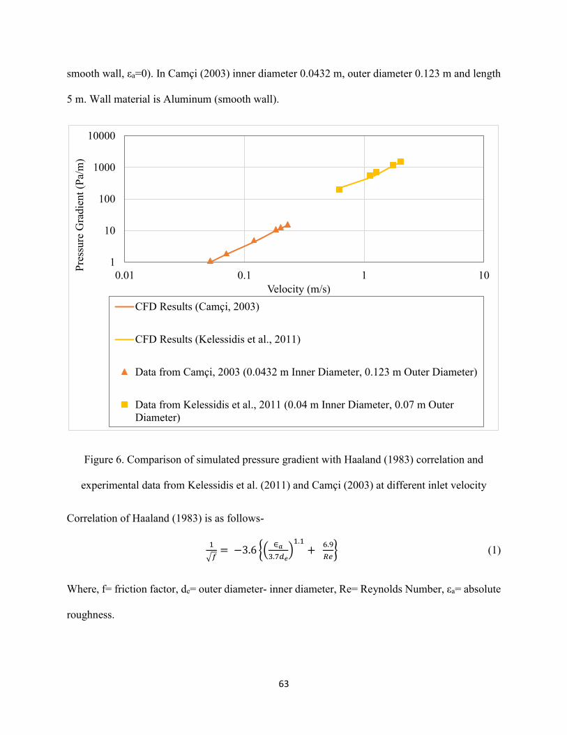
63

smooth wall, εa=0). In Camçi (2003) inner diameter 0.0432 m, outer diameter 0.123 m and length

5 m. Wall material is Aluminum (smooth wall).

Figure 6. Comparison of simulated pressure gradient with Haaland (1983) correlation and

experimental data from Kelessidis et al. (2011) and Camçi (2003) at different inlet velocity

Correlation of Haaland (1983) is as follows-

1

√𝑓= −3.6 (

∈𝑎

3.7𝑑𝑒)1.1

+ 6.9

𝑅𝑒 (1)

Where, f= friction factor, de= outer diameter- inner diameter, Re= Reynolds Number, εa= absolute

roughness.

1

10

100

1000

10000

0.01 0.1 1 10

Pre

ssure

Gra

die

nt

(Pa/

m)

Velocity (m/s)

CFD Results (Camçi, 2003)

CFD Results (Kelessidis et al., 2011)

Data from Camçi, 2003 (0.0432 m Inner Diameter, 0.123 m Outer Diameter)

Data from Kelessidis et al., 2011 (0.04 m Inner Diameter, 0.07 m Outer

Diameter)

64

In Figure 6, the graph represents log-log scale. Pressure gradient increasing rate in log-log scale is

almost linear for both cases. The average percentage error of simulation results from Kelessidis et

al. (2011) and Camçi (2003) are 9.88% and 8.46% respectively which indicates very good

agreement (it was estimated that the error of the experimental data is approximately ±10% in

Kelessidis et al. 2011).

Two Phase (solid-liquid) flow through Annuli

Pressure gradient (Pa/m) profile of water-sand slurry flow through vertical concentric annuli is

compared with Ozbelge and Beyaz (2001) [35] experimental data in Figure 7. For the CFD

simulation, the liquid phase is considered as water (density 9982 kg/m3, viscosity 0.001003 kg/m-

s) and solid phase is taken as feldspar (symbol K2O.Al2O3.SiO2, mean particle diameter 0.23 mm,

mean density 2500 kg/m3). Length 5 m, outer diameter 0.125 m, inner diameter 0.025 m, inlet

velocity range of 0.0738–0.197 m/s and overall slurry volumetric concentration range of 0.8%–

1.8% with 0.23 mm grain size (dp) are considered as boundary conditions. A smooth pipe of

stainless steel (density 8030 kg/m3) is used for the simulation. The pipe is assumed to be vertical,

i.e., gravity effect is included and gravity acceleration is directed opposite to outlet. No slip

condition for liquid and solid phase is used at the walls. Figure 14 shows the comparison of

simulated and experimental two-phase frictional pressure drop through vertical annuli at different

mixture velocity and at different volume concentration of slurry for 0.23 mm mean sand particle

diameter (dp). Simulated results are in good agreement with experimental values with 2.62%

average error.

65

Figure 7. Comparison of simulated two-phase frictional pressure gradient at different mixture

velocity and volume concentration of slurry with Ozbelge and Beyaz, 2001 (0.125 m outer

diameter, 0.025 m inner diameter, dm = 0.23 mm) [dm = sand particle diameter, Cv = sand

volumetric concentrations]

Results and Discussion

After achieving good validation of proposed model with experimental data, parametric analysis

is done to observe the effect of changing flow rate, drill pipe rotation, eccentricity and particle

size. (data tables are presented in Appendix 4).

0

50

100

150

200

250

300

350

400

0 0.05 0.1 0.15 0.2 0.25

Pre

ssure

Gra

die

nt

(Pa/

m)

Mixture Velocity (m/s)

CFD Results (volume concentration 1.8% v/v)CFD Results (volume concentration 1.5% v/v)CFD Results (volume concentration 1.0% v/v)CFD Results (volume concentration 0.8% v/v)Experiment (volume concentration 1.8% v/v)Experiment (volume concentration 1.5% v/v)Experiment (volume concentration 1.0% v/v)Experiment (volume concentration 0.8% v/v)

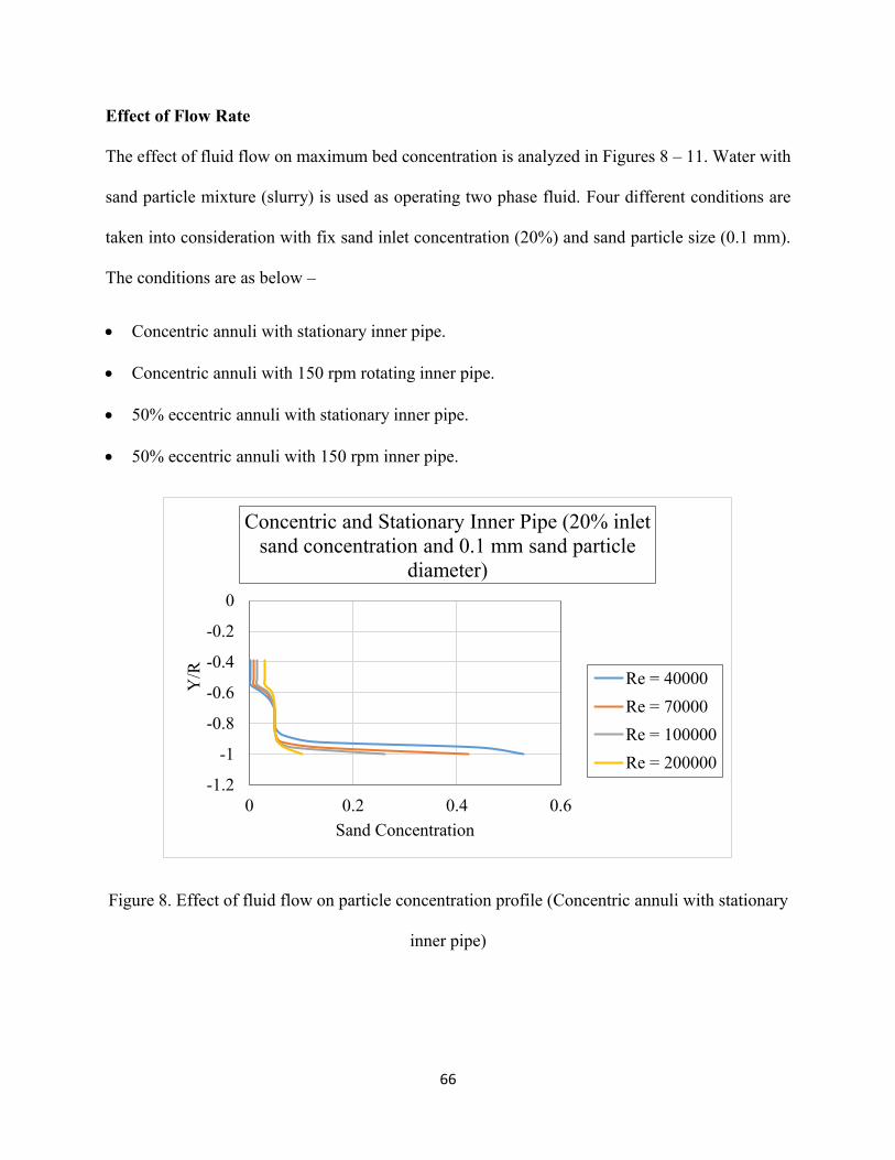
66

Effect of Flow Rate

The effect of fluid flow on maximum bed concentration is analyzed in Figures 8 – 11. Water with

sand particle mixture (slurry) is used as operating two phase fluid. Four different conditions are

taken into consideration with fix sand inlet concentration (20%) and sand particle size (0.1 mm).

The conditions are as below –

• Concentric annuli with stationary inner pipe.

• Concentric annuli with 150 rpm rotating inner pipe.

• 50% eccentric annuli with stationary inner pipe.

• 50% eccentric annuli with 150 rpm inner pipe.

Figure 8. Effect of fluid flow on particle concentration profile (Concentric annuli with stationary

inner pipe)

-1.2

-1

-0.8

-0.6

-0.4

-0.2

0

0 0.2 0.4 0.6

Y/R

Sand Concentration

Concentric and Stationary Inner Pipe (20% inlet

sand concentration and 0.1 mm sand particle

diameter)

Re = 40000

Re = 70000

Re = 100000

Re = 200000

67

Figure 9. Effect of fluid flow on particle concentration profile (Concentric annuli with 150 rpm

rotating inner pipe)

Figure 10. Effect of fluid flow on particle concentration profile (50% eccentric annuli with

stationary inner pipe)

-1.2

-1

-0.8

-0.6

-0.4

-0.2

0

0 0.2 0.4 0.6

Y/R

Sand Concentration

Concentric and 150 rpm Rotating Inner Pipe (20%

inlet sand concentration and 0.1 mm sand particle

diameter)

Re = 40000

Re = 70000

Re = 100000

Re = 200000

-1.2

-1

-0.8

-0.6

-0.4

-0.2

0

0 0.1 0.2 0.3 0.4

Y/R

Sand Concentration

50% Eccentric and Stationary Inner Pipe (20% inlet

sand concentration and 0.1 mm sand particle

diameter)

Re = 85000

Re = 100000

Re = 200000

Re = 300000

68

Figure 11. Effect of fluid flow on particle concentration profile (50% eccentric annuli with 150

rpm inner pipe)

The analysis is done near bottom wall. In each case, with the increase of flow rate bed

concentration near wall decrease. Due to gravitational force and horizontal orientation sand

particles have the tendency to gather near bottom wall and create a flow blockage. Decreasing flow

enhance the process. From the analysis it is found that below 9*104 Reynolds number bed

concentration near bottom wall is more than 25% in all cases and when it goes down 4*104 the

percentage is above 50%. In Figure 12, sample contour distribution of sand particles is shown at

different flow rate. Operating conditions are taken from Figure 8. Contour distribution of annuli

cross section at 3 m distance from inlet, displays the effect of fluid flow and gravitational force on

concentration distribution clearly.

-1.2

-1

-0.8

-0.6

-0.4

-0.2

0

0 0.1 0.2 0.3

Y/R

Sand Concentration

50% Eccentric and 150 rpm Rotating Inner Pipe

(20% inlet sand concentration and 0.1 mm sand

particle diameter)

Re = 85000

Re = 100000

Re = 200000

Re = 300000

69

(a)

(b)

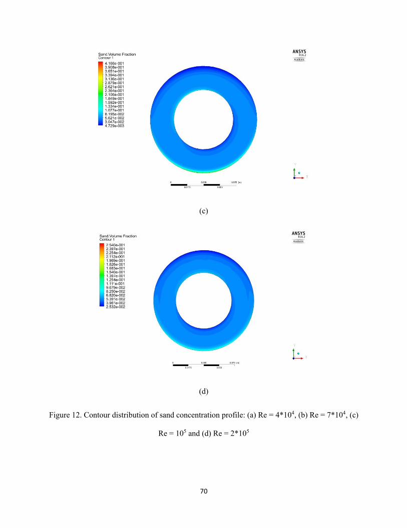
70

(c)

(d)

Figure 12. Contour distribution of sand concentration profile: (a) Re = 4*104, (b) Re = 7*104, (c)

Re = 105 and (d) Re = 2*105

71

Effect of Drill Pipe Rotation and Eccentricity

Inner pipe of annuli can affect pressure loss by changing its eccentricity and rotation. The effect

of inner pipe rotation and eccentricity are presented in Figure 13 and 14. Single phase water is

used as fluid in this analysis. From Figure 13, it can be visualized that pressure loss increases with

the increase of rotational speed and this trend is same at different flow rates. Stationary, 50 rpm,

100 rpm and 150 rpm rotation of inner pipe is taken into consideration. Increasing trend is higher

at high flow rates. Due to rotational speed particle – particle and particle – wall collision and

rebound increases which results in higher pressure loss.

Figure 13. Effect of inner pipe rotation on pressure loss

Figure 14 shows the effect of inner pipe eccentricity on pressure loss. Concentric, 25%

eccentricity, 50% eccentricity and 75% eccentricity are analyzed in this figure. At a fixed flow rate

(Re = 50000), with the increase of inner pipe eccentricity pressure loss decreases. This trend is

applicable during inner pipe stationary condition. With inner pipe rotation, the trend is opposite.

Due to extra collision added by pipe rotation this change occurs.

0

200

400

600

800

1000

1200

0 50 100 150 200

Pre

ssure

loss

(P

a/m

)

Rotational speed (rpm)

Re = 20000

Re = 40000

Re = 50000

Re = 60000

Re = 80000

Re = 100000

72

Figure 14. Effect of inner pipe eccentricity on pressure loss at different rotational speed

Effect of Particle Size

In slurry flow, sand particle size has effective role on particle blockage near bottom wall of

horizontal annular pipe. Figure 15 analyzes the effect of sand particle size at concentric and

stationary inner pipe with 5% inlet sand concentration. With the increase of sand particle size,

particle deposition near bottom wall increases. With the increase of size, individual particle weight

increases which eventually results this blockage. From previous analysis we have found maximum

bed concentration decreases with the increase of flow rate (Figures 7 – 11) but for particle size

0.005 mm, maximum bed concentration near bottom wall is almost constant at different flow rates.

That means, for smaller particle size (< 0.01 mm) the effect of flow rate on particle deposition has

been reduced to a negligible level.

0

100

200

300

400

500

600

0 50 100 150 200

Pre

ssure

loss

(P

a/m

)

Rotational speed (rpm)

Re = 50000

ecc = 0%

ecc = 25%

ecc = 50%

ecc = 75%

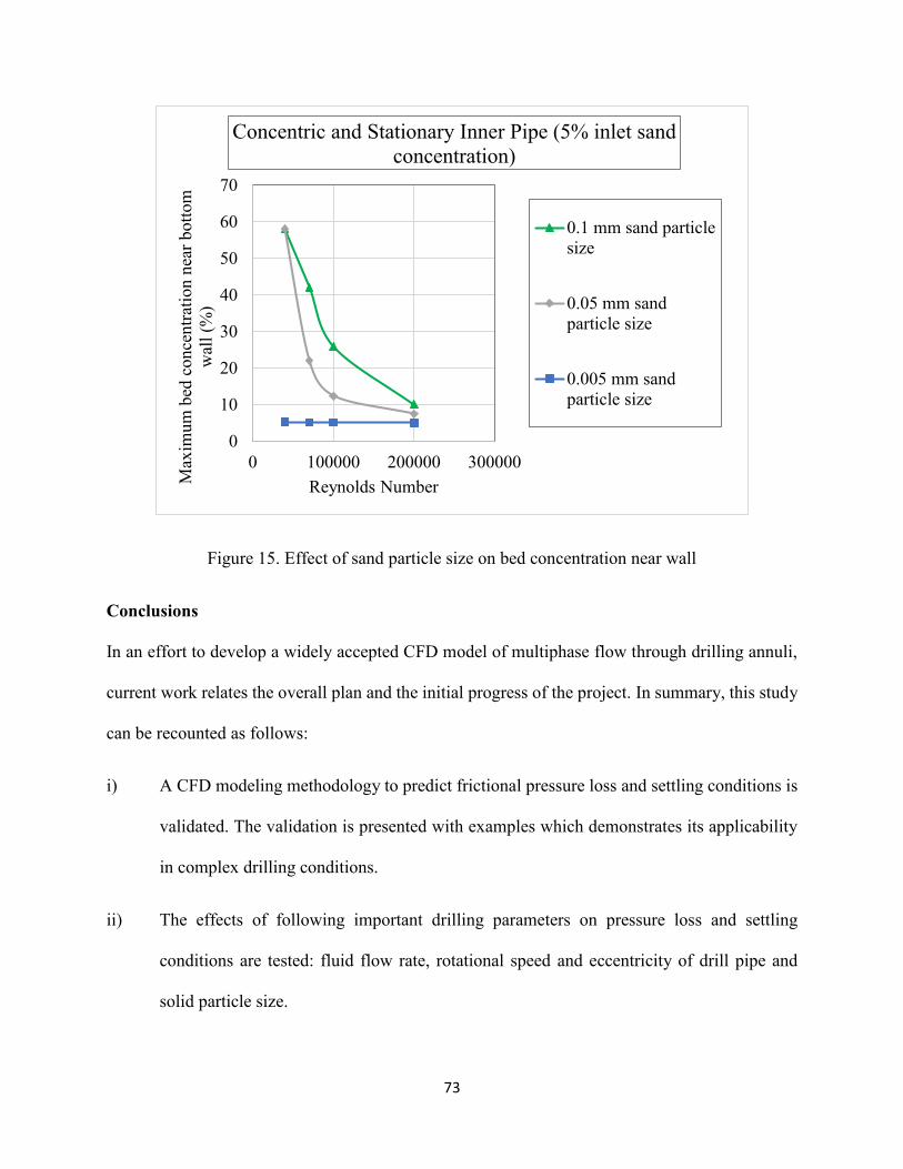
73

Figure 15. Effect of sand particle size on bed concentration near wall

Conclusions

In an effort to develop a widely accepted CFD model of multiphase flow through drilling annuli,

current work relates the overall plan and the initial progress of the project. In summary, this study

can be recounted as follows:

i) A CFD modeling methodology to predict frictional pressure loss and settling conditions is

validated. The validation is presented with examples which demonstrates its applicability

in complex drilling conditions.

ii) The effects of following important drilling parameters on pressure loss and settling

conditions are tested: fluid flow rate, rotational speed and eccentricity of drill pipe and

solid particle size.

0

10

20

30

40

50

60

70

0 100000 200000 300000

Max

imum

bed

conce

ntr

atio

n n

ear

bott

om

wal

l (%

)

Reynolds Number

Concentric and Stationary Inner Pipe (5% inlet sand

concentration)

0.1 mm sand particle

size

0.05 mm sand

particle size

0.005 mm sand

particle size

74

iii) Preliminary results of current research program are presented. The project is expected to

produce a comprehensive CFD model capable of considering all important drilling

parameters.

References

[1]. Pilehvari, A. and R. Serth, Generalized hydraulic calculation method for axial flow of non-

Newtonian fluids in eccentric annuli. SPE drilling & completion, 24(04), (2009). 553-563.

[2]. Reed, T. and A. Pilehvari, 1993. "A new model for laminar, transitional, and turbulent flow

of drilling muds". In Proceedings of SPE Production Operations Symposium, Society of

Petroleum Engineers.

[3]. Anifowoshe, O.L. and S.O. Osisanya, 2012. "The Effect of Equivalent Diameter Definitions

on Frictional Pressure Loss Estimation in an Annulus with Pipe Rotation". In Proceedings of

SPE Deepwater Drilling and Completions Conference, Society of Petroleum Engineers.

[4]. Ahmed, R.M., M.S. Enfis, H.M. El Kheir, M. Laget, and A. Saasen, 2010. "The Effect of

Drillstring Rotation on Equivalent Circulation Density: Modeling and Analysis of Field

Measurements". In Proceedings of SPE Annual Technical Conference and Exhibition,

Society of Petroleum Engineers.

[5]. Dosunmu, I.T. and S.N. Shah, Evaluation of friction factor correlations and equivalent

diameter definitions for pipe and annular flow of non-Newtonian fluids. Journal of Petroleum

Science and Engineering, 109, (2013). 80-86.

[6]. Erge, O., E.M. Ozbayoglu, S.Z. Miska, M. Yu, N. Takach, A. Saasen, and R. May, Equivalent

circulating density modeling of Yield Power Law fluids validated with CFD approach.

Journal of Petroleum Science and Engineering, 140, (2016). 16-27.

75

[7]. Hansen, S.A. and N. Sterri, 1995. "Drill Pipe Rotation Effects on Frictional Pressure Losses

in Slim Annuli". In Proceedings of SPE Annual Technical Conference and Exhibition,

Society of Petroleum Engineers.

[8]. Sorgun, M., Computational Fluid Dynamics Modeling of Pipe Eccentricity Effect on Flow

Characteristics of Newtonian and Non-Newtonian Fluids. Energy Sources, Part A: Recovery,

Utilization, and Environmental Effects, 33(12), (2011). 1196-1208.

[9]. Sorgun, M. and M. Ozbayoglu, Predicting Frictional Pressure Loss During Horizontal

Drilling for Non-Newtonian Fluids (vol 33, pg 631, 2011). Energy Sources Part A-recovery

Utilization and Environmental Effects, 33(11), (2011). 1104-1106.

[10]. Subramanian, R. and J. Azar, 2000. "Experimental study on friction pressure drop for

nonnewtonian drilling fluids in pipe and annular flow". In Proceedings of International Oil

and Gas Conference and Exhibition in China, Society of Petroleum Engineers.

[11]. Camçi, G. and T.A. Özbelge, Determination of dilute slurry densities in a vertical annulus

using isokinetic sampling. Chem. Eng. Comm., 193(11), (2006). 1482-1501.

[12]. Dewangan, S.K. and S.L. Sinha, Exploring the hole cleaning parameters of horizontal

wellbore using two-phase Eulerian CFD approach. The Journal of Computational Multiphase

Flows, 8(1), (2016). 15-39.

[13]. Özbelge, T.A. and A.N. Eraslan, A computational hydrodynamic and heat transfer study in

turbulent up-flows of dilute slurries through a concentric annulus. Turkish Journal of

Engineering and Environmental Sciences, 30(1), (2006). 1-13.

[14]. Özbelge, T.A. and G.C. Ünal, A new correlation for two-phase pressure drops in fully

developed dilute slurry up-flows through an annulus. Chemical Engineering

Communications, 196(4), (2008). 491-498.

76

[15]. Ofei, T.N., Effect of Yield Power Law Fluid Rheological Properties on Cuttings Transport

in Eccentric Horizontal Narrow Annulus. Journal of Fluids, 2016, (2016).

[16]. Sorgun, M. and E. Ulker, Modeling and Experimental Study of Solid-Liquid Two-Phase

Pressure Drop in Horizontal Wellbores with Pipe Rotation. Journal of Energy Resources

Technology-Transactions of the Asme, 138(2), (2016).

[17]. Sun, X., K. Wang, T. Yan, S. Shao, and J. Jiao, Effect of drillpipe rotation on cuttings

transport using computational fluid dynamics (CFD) in complex structure wells. Journal of

Petroleum Exploration and Production Technology, 4(3), (2014). 255-261.

[18]. Alder, B. and T. Wainwright, Studies in molecular dynamics. II. Behavior of a small number

of elastic spheres. The Journal of Chemical Physics, 33(5), (1960). 1439-1451.

[19]. Chapman, S. and T.G. Cowling, The mathematical theory of non-uniform gases: an account

of the kinetic theory of viscosity, thermal conduction and diffusion in gases: Cambridge

university press, 1970.

[20]. Syamlal, M., W. Rogers, and T.J. O’Brien, MFIX documentation: Theory guide. National

Energy Technology Laboratory, Department of Energy, Technical Note DOE/METC-

95/1013 and NTIS/DE95000031, (1993).

[21]. Anderson, T.B. and R. Jackson, Fluid mechanical description of fluidized beds. Equations of

motion. Industrial & Engineering Chemistry Fundamentals, 6(4), (1967). 527-539.

[22]. Bowen, R.M., Theory of mixtures. Continuum physics, 3(Part I), (1976).

[23]. Patankar, S., Numerical heat transfer and fluid flow: CRC press, 1980.

[24]. Vasquez, S. and V. Ivanov, 2000. "A phase coupled method for solving multiphase problems

on unstructured meshes". In Proceedings of ASME 2000 Fluids Engineering Division

Summer Meeting (ASME FEDSM’00), paper FEDSM2000-11281, pp. 1-6.

77

[25]. Weiss, J.M., J.P. Maruszewski, and W.A. Smith, Implicit solution of preconditioned Navier-

Stokes equations using algebraic multigrid. AIAA journal, 37(1), (1999). 29-36.

[26]. Barth, T. and D. Jespersen, The design and application of upwind schemes on unstructured

meshes, 27th Aerospace Sciences MeetingAmerican Institute of Aeronautics and

Astronautics 1989.

[27]. Gibson, M. and B. Launder, Ground effects on pressure fluctuations in the atmospheric

boundary layer. Journal of fluid mechanics, 86(03), (1978). 491-511.

[28]. Launder, B., G.J. Reece, and W. Rodi, Progress in the development of a Reynolds-stress

turbulence closure. Journal of fluid mechanics, 68(03), (1975). 537-566.

[29]. Launder, B.E., Second‐moment closure and its use in modelling turbulent industrial flows.

International Journal for Numerical Methods in Fluids, 9(8), (1989). 963-985.

[30]. Chorin, A.J., Numerical solution of the Navier-Stokes equations. Mathematics of

computation, 22(104), (1968). 745-762.

[31]. Brown, N.P. and N.I. Heywood, Slurry Handling: Design of solid-liquid systems: Springer

Science & Business Media, 1991.

[32]. Wasp, E.J., J.P. Kenny, and R.L. Gandhi, Solid--liquid flow: slurry pipeline transportation.

[Pumps, valves, mechanical equipment, economics]. Ser. Bulk Mater. Handl.;(United States),

1(4), (1977).

[33]. Kelessidis, V.C., P. Dalamarinis, and R. Maglione, Experimental study and predictions of

pressure losses of fluids modeled as Herschel–Bulkley in concentric and eccentric annuli in

laminar, transitional and turbulent flows. Journal of Petroleum Science and Engineering,

77(3), (2011). 305-312.

78

[34]. Haaland, S.E., Simple and explicit formulas for the friction factor in turbulent pipe flow.

Journal of Fluids Engineering, 105(1), (1983). 89-90.

[35]. Özbelge, T. and A. Beyaz, Dilute solid–liquid upward flows through a vertical annulus in a

closed loop system. International Journal of Multiphase Flow, 27(4), (2001). 737-752.

[36]. Dyakowski, T., L.F.C. Jeanmeure, and A.J. Jaworski, Applications of electrical tomography

for gas–solids and liquid–solids flows — a review. Powder Technology, 112(3), (2000). 174-

192.

[37]. Lucas, G., J. Cory, R. Waterfall, W. Loh, and F. Dickin, Measurement of the solids volume

fraction and velocity distributions in solids–liquid flows using dual-plane electrical resistance

tomography. Flow Measurement and Instrumentation, 10(4), (1999). 249-258.

[38]. Na, W., J.B. Jia, X. Yu, Y. Faraj, Q. Wang, Y.F. Meng, M. Wang, and W.T. Sun, Imaging of

gas-liquid annular flows for underbalanced drilling using electrical resistance tomography.

Flow Measurement and Instrumentation, 46, (2015). 319-326.

[39]. Tan, C., S.-J. Ren, and F. Dong, Reconstructing the phase distribution within an annular

channel by electrical resistance tomography. Heat Transfer Engineering, 36(12), (2015).

1053-1064.

[40]. Kaushal, D. R., Kimihiko Sato, Takeshi Toyota, Katsuya Funatsu, and Yuji Tomita. "Effect

of particle size distribution on pressure drop and concentration profile in pipeline flow of

highly concentrated slurry." International Journal of Multiphase Flow 31, no. 7 (2005): 809-

823.

[41]. Camçı, Gülden. "Application of isokinetic sampling technique for local solid densities in

upward liquid-solid flows through an annulus." PhD diss., METU, 2003.

79

[42]. Skudarnov, P. V., C. X. Lin, and M. A. Ebadian. "Double-species slurry flow in a horizontal

pipeline." Journal of fluids engineering 126, no. 1 (2004): 125-132.

80

Chapter 3. CFD Simulation of Three Phase Gas-Liquid-Solid Flow in

Horizontal Pipes

Rasel A Sultan



St. John’s, NL, Canada

[email protected]

M. A. Rahman




[email protected]

Sohrab Zendehboudi




[email protected]

Vassilios C. Kelessidis

Petroleum Institute

Department of Petroleum Engineering

Abu Dhabi, UAE

[email protected]

Abstract

The objective of this work is to analyze fluid flow in horizontal pipes with three phase gas-liquid-

solid Newtonian fluid by our developed CFD simulation model and validate the simulation with

experimental works. Air as gas, water as liquid and silica sand as solid particle is used for this

work. ANSYS fluent version 16.2 is used to do the simulation. Eulerian model with Reynolds

Stress Model (RSM) turbulence closure is adopted to analyze multiphase fluid flow. Length of

pipe is 2.9 m and diameter is 0.0416 m, which are selected from experimental works to validate

the simulation and after a good agreement with experimental data, sensitivity analysis is conducted

to observe the three phase fluid flow characteristics through horizontal flow. Pressure gradient

(pressure drop per unit length) is used as primary parameter to analyze. Effect of in situ

concentration of solid in slurry, diameter of pipeline, roughness of wall material and viscosity of

water in slurry are analyzed throughout this paper. This article provides validity of our proposed

model. After that we tried to perform some parametric studies, changing variables of three phase

mailto:[email protected]




81

fluid flow through horizontal pipeline with ours validated model. The main approach here is to

demonstrate our CFD model in different ways to researchers and industries related to multiphase

pipeline flow fields and make it acceptable to them. Also, Fluid Structure Interaction (FSI) is

introduced at the end of this study to explain the goal of this project.

Introduction

Gas-liquid-solid three phase flow in pipeline or annuli has great interest in oil and gas industries

to recover produced formation fluid [1], mining [2, 3], biomass transportation [4], horizontal

petroleum production and transport [5], nuclear waste deposition [6]. The addition of solid

particles to two phase air-water flow can reduce drag in pipe flow which can lead to decreasing

pressure drop and pumping power [7], and also decreasing the size of pump [8]. The three phase

slurry transportation with air and water helps to reduce air pollution, noise, accidents and energy

demand. Also adding air or air injection in two phase slurry system reduce pumping cost and

enhance bitumen recovery from oil field [9].

There are extensive experimental studies in this field [5-6, 8, 10-29], focusing on pressure gradient,

deposition velocity (i.e. minimum superficial velocity of mixture to restrain gathering of solids or

wastes in the pipeline), and the in-situ concentration of different phases. But these works are

representing with narrow range of operating conditions and incomplete due to having minimum

number of measurements. [27]. For example, Gillies et al. only focused on pressure gradients and

in situ concentration of fluids [19]; Fukuda and Shoji elaborated pressure gradient only [14].

The CFD simulation of solid-liquid-gas three phase flow are limited to a few [29-33]. Also those

studies are limited to small ranges of analysis. For example, Li et al. studied CFD simulation of

solid-liquid-gas three phase flow to analyze hydraulic transport process through pipeline but with

limited ranges [29].

82

CFD approach with three phase pipeline flow can be used to find more effective outputs and so it

is considered appropriate to use for this study. Eulerian multiphase model for phase mixture

behavior along with Reynolds Stress Model (RSM) for turbulence behavior are deliberated in our

proposed model. These combination shows optimum and more accurate results. There is few

acceptable commercial software available to perform multiphase fluid flow. ANSYS fluid is used

to perform the analysis.

In this study, we compare the CFD simulation with experimental studies at different conditions

and ranges with horizontal pipe. After verifying our simulation model, parametric study is

conducted with a good range of variable. These parametric studies are also verified with available

correlations to demonstrate high reliance on this proposed model at different applications and

different conditions in present and future works related to pipe flow with multiphase fluids.

Mathematical Model

The Euler-Euler approach is considered for each phase, in contrast to the Eulerian-Lagrangian

model that calculate solid phase with individual discrete calculations. The Eulerian model from

Euler-Euler approach is used here as multiphase model. In our work, we have solid-liquid-gas

fluids where granular (solid-liquid) flow is expected to be in a high range. Due to this high range

of solid phase the Eulerian model is selected as optimum and effective in our case.

The volume of phase 𝑞, is defined by


where,

83

∑ 𝑎𝑞 = 1𝑛𝑞=1 (2)

Continuity equation for mixture is as below -

𝜕

𝜕𝑡(𝑎𝑞𝜌𝑞) + ∇. (𝑎𝑞𝜌𝑞𝜗𝑞 ) = 0 (3)

where, 𝜌𝑞 is the phase reference density, or the volume averaged density of the 𝑞𝑡ℎ phase in the

solution domain. 𝜗𝑞 indicates velocity vector.

The momentum equation for a fluid phase 𝑞 is -

𝜕


𝑛𝑝=1


Here, 𝑔 is the acceleration due to gravity, 𝜏 is the 𝑞𝑡ℎ phase stress-strain tensor, 𝐹𝑞 is an external


Following the work of Alder and Wainwrigh (1960) [34], Chapman and Cowling (1970) [35] and

Syamlal et al. (1993) [36], a multi-fluid granular model is used to describe the flow behavior of a

fluid-solid mixture.

The conservation of momentum for the solid phase is -

𝜕


𝑁𝑙=1


where, 𝑝𝑠 is the 𝑠𝑡ℎ solids pressure, 𝐾𝑙𝑠 = 𝐾𝑠𝑙 is the momentum exchange coefficient between


84

The solids pressure term consists of a kinetic term and a second particle collisions term -


where, 𝑒𝑠𝑠 is the coefficient of restitution for particle collisions, 𝑔0,𝑠𝑠 is the radial distribution

function, and 𝛩𝑠 is the granular temperature. The solids stress viscosity term contains or shear

viscosity due to collision (𝜇𝑠,𝑐𝑜𝑙), kinetic viscosity (𝜇𝑠,𝑘𝑖𝑛) and frictional viscosity (𝜇𝑠,𝑓𝑟). So, it

can be written as -


where, 𝜇𝑠,𝑐𝑜𝑙 is shear viscosity due to collision, 𝜇𝑠,𝑘𝑖𝑛 is kinetic viscosity and 𝜇𝑠,𝑓𝑟 frictional

viscosity.

Previous studies and literatures indicate few comparisons between all the turbulence models like

Reynolds-averaged Navier–Stokes (RANS) models: k–ɛ, k–ω and Reynolds stress model, and

Large Eddy Simulation (LES) for steady fluid flow through pipeline or annuli [37]. In Vijiapurapu

and Cui [37] results obtained with different turbulence models were compared with experimental

results from Zagarola and Smits [38] and Nourmohammadi et al. [39]. The k–ɛ and k–ω models

can provide acceptable accurate result with low computational cost and least effort. On the other

hand, LES model solves large scales of turbulence with smallest scales and so it is more universal

and acceptable model, but it takes higher computational cost with higher computational time [37].

Among all these turbulence model Reynolds Stress Model (RSM) is optimum to use for turbulence

flow through simple pipe or annuli. RSM needs less computational time or computational cost than

LES model and gives more accurate result than k–ɛ and k–ω models [37]. For example, RSM can

calculate directional effects of the Reynolds stress field that can not be done by other Reynolds-

averaged Navier–Stokes (RANS) models.

85

An analysis with different turbulence model is conducted using data from Kaushal et al. (2005)

[40] to find out optimum model for further investigations. In Fig. 1, single phase water velocity 1

m/s is maintained through horizontal pipeline. The analysis shows RSM as the most optimum

model with least error.

Considering above comparisons RSM is considered here as turbulence model for multiphase fluid

flow. RSM solves the Reynolds-averaged Navier-Stokes equation by solving transport equations

for the Reynolds stresses, together with an equation for the dissipation rate.

Figure 1. Optimum turbulence model analysis

Modelling approach of RSM is originated in 1975 by Launder et al. [41]. The exact transport

equation of Reynolds Stress (𝑅𝑖𝑗 𝑜𝑟 𝑢𝑖′𝑢𝑗′ ) is as below -

𝐷𝑅𝑖𝑗

𝐷𝑡= 𝑃𝑖𝑗 + 𝐷𝑖𝑗 − 휀𝑖𝑗 + ∅𝑖𝑗 + 𝜃𝑖𝑗 (8)

Here,

𝐷𝑅𝑖𝑗

𝐷𝑡 is the summation of changing rate of 𝑅𝑖𝑗 and transport of 𝑅𝑖𝑗 by convection.

180

200

220

240

Experiment Reynolds

Stress

Model

Standard K-

Omega

Model

SST K-

Omega

Model

Pre

ssure

Gra

die

nt

(Pa/

m)

86

𝑃𝑖𝑗 is production rate of 𝑅𝑖𝑗.

𝐷𝑖𝑗 is diffusion transport of 𝑅𝑖𝑗.

휀𝑖𝑗 is rate of dissipation.

∅𝑖𝑗 is pressure strain correlation term.

𝜃𝑖𝑗 is rotation term.

𝐷 𝑖𝑗 can be modeled assuming rate of transport of Reynolds stresses by diffusion is proportional

to gradients of Reynolds stresses. Diffusion term used in simulation is as below -



𝜎𝑘

𝜕𝑅𝑖𝑗

𝜕𝑥𝑘) (9)

where, 𝜎𝑘 = 0.82 [42], 𝜇𝑡 = 𝐶𝜇𝑘2

𝜖 𝑎𝑛𝑑 𝐶𝜇 = 0.09.

Production rate 𝑃𝑖𝑗 of 𝑅𝑖𝑗 𝑜𝑟 𝑢𝑖′𝑢𝑗′ can be expressed as -

𝑃𝑖𝑗 = − (𝑢𝑖′𝑢𝑚′ 𝜕𝑈𝑗𝜕𝑥𝑚

+ 𝑢𝑗′𝑢𝑚′ 𝜕𝑈𝑖𝜕𝑥𝑚

) (10)

The pressure-strain term, ∅𝑖𝑗 on Reynold stresses consists of three major components [43, 44] and

those are ∅𝑖𝑗,1 or slow pressure-strain term also known as the return-to-isotropy term, ∅𝑖𝑗,2 or

rapid pressure-strain term and ∅𝑖𝑗,𝑤 as wall-reflection term. So, it can be presented as –

∅𝑖𝑗 = ∅𝑖𝑗,1 + ∅𝑖𝑗,2 + ∅𝑖𝑗,𝑤 (11)

where,

∅𝑖𝑗,1 = −𝐶1𝜖


2

3𝛿𝑖𝑗𝑘] (12)

∅𝑖𝑗,2 = −𝐶2 [𝑃𝑖𝑗 − 2

3𝛿𝑖𝑗𝑃] (13)

87

With, 𝐶1 = 1.8 and 𝐶2 = 0.6

The wall-reflection term, ∅𝑖𝑗,𝑤 is responsible for the normal stresses distribution near the wall.

This term is modeled as -

∅𝑖𝑗,𝑤 ≡ 𝐶1′𝜖

𝑘(𝑢𝑘′ 𝑢𝑚′ 𝑛𝑘𝑛𝑚𝛿𝑖𝑗 −

3

2𝑢𝑖′𝑢𝑘

′ 𝑛𝑗𝑛𝑘 − 3

2𝑢𝑗′𝑢𝑘

′ 𝑛𝑖𝑛𝑘)𝐶𝑙𝑘

32

𝜖𝑑+ 𝐶2

′(∅𝑘𝑚,2𝑛𝑘𝑛𝑚𝛿𝑖𝑗

− 3

2∅𝑖𝑘,2𝑛𝑗𝑛𝑘 −

3

2∅𝑗𝑘,2𝑛𝑖𝑛𝑘)

𝐶𝑙𝑘32

𝜖𝑑 (14)

where, 𝐶1′ = 0.5, 𝐶2

′ = 0.3, 𝑛𝑘 is the horizontal component of the component normal to the wall,

𝑑 is the shortest distance to the wall, and 𝐶𝑙 = 𝐶𝜇

34

𝑘, where 𝐶𝜇 = 0.09 and 𝑘 is the von Kármán

constant (=0.4187).

The dissipation rate 𝜖𝑖𝑗 or destruction rate of 𝑅𝑖𝑗, is modeled as -

𝜖𝑖𝑗 = 2

3𝛿𝑖𝑗𝜖 (15)

where,

𝜖 = 2𝑣𝑠𝑖𝑗′ . 𝑠𝑖𝑗′ (16)

and 𝑠𝑖𝑗′ = fluctuating deformation rate

Rotation term is expressed as –

𝜃𝑖𝑗 = −2𝜔𝑘(𝑅𝑗𝑚𝑒𝑖𝑘𝑚 + 𝑅𝑖𝑚𝑒𝑗𝑘𝑚) (17)

Here,

𝜔𝑘= rotation vector.

𝑒𝑖𝑘𝑚=alternating symbol, +1, -1 or 0 depending on i, j and k.

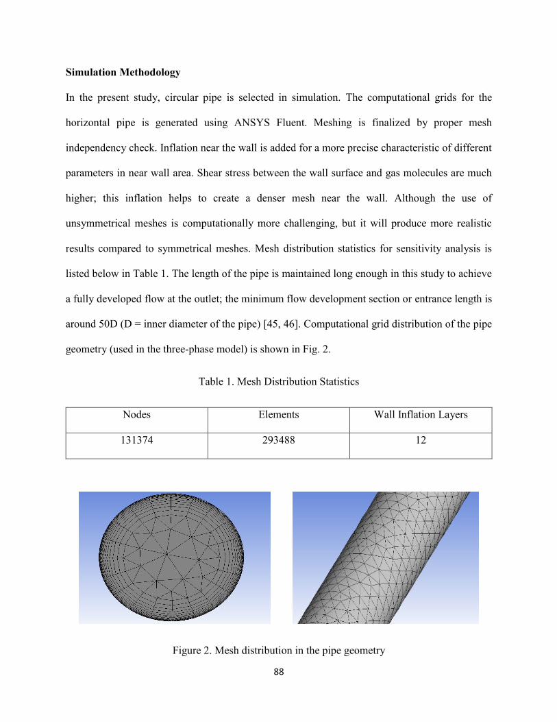
88


In the present study, circular pipe is selected in simulation. The computational grids for the

horizontal pipe is generated using ANSYS Fluent. Meshing is finalized by proper mesh

independency check. Inflation near the wall is added for a more precise characteristic of different

parameters in near wall area. Shear stress between the wall surface and gas molecules are much

higher; this inflation helps to create a denser mesh near the wall. Although the use of

unsymmetrical meshes is computationally more challenging, but it will produce more realistic

results compared to symmetrical meshes. Mesh distribution statistics for sensitivity analysis is

listed below in Table 1. The length of the pipe is maintained long enough in this study to achieve

a fully developed flow at the outlet; the minimum flow development section or entrance length is

around 50D (D = inner diameter of the pipe) [45, 46]. Computational grid distribution of the pipe

geometry (used in the three-phase model) is shown in Fig. 2.

Table 1. Mesh Distribution Statistics

Nodes Elements Wall Inflation Layers

131374 293488 12

Figure 2. Mesh distribution in the pipe geometry

89

Fluent, ver. 16.2, ANSYS Inc. is used to build a CFD simulation model of the pipeline flow of air-

water-sand slurry. In solution, a convergence value of 10-5 is used to terminate the iterations, this

threshold value is selected after optimization to ensure a satisfactory accuracy at the lowest

computation time. Figure 3. shows an analysis to find out optimum convergence rate (between a

range of 10-4 to 10-6) using parameters (inlet velocity) from experiment. In average, 20 minutes’

computational time was counted for each simulation of this project. SIMPLE algorithm is applied

with first and second order upwind discretization method to have stability and confirm

convergence in governing equations. Upwind discretization is such a method that simulate

numerically the direction of the normal velocity in the flow field. No-slip boundary condition is

adopted for interaction between solid or liquid phase and wall.

Figure 3. Optimum convergence rate analysis

Simulation Validation

The CFD simulation is first verified using single phase flow of water with experimental data from

Skudarnov et al. [47], and the empirical correlation of Wood’s [48]. Here, the geometry of pipe,

fluid and wall material is taken similar to Skudarnov et al.; we use the pipe length of 17 m, and

0

1

2

3

4

5

1.E-07 1.E-06 1.E-05 1.E-04

Pre

ssure

Gra

die

nt

(Pa/

m)

Convergent Rate

v=0.12 m/s

v=0.0707 m/s

v=0.0516 m/s

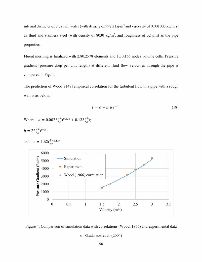
90

internal diameter of 0.023 m, water (with density of 998.2 kg/m3 and viscosity of 0.001003 kg/m.s)

as fluid and stainless steel (with density of 8030 kg/m3, and roughness of 32 µm) as the pipe

properties.

Fluent meshing is finalized with 2,80,2578 elements and 1,30,165 nodes volume cells. Pressure

gradient (pressure drop per unit length) at different fluid flow velocities through the pipe is

compared in Fig. 4.

The prediction of Wood’s [48] empirical correlation for the turbulent flow in a pipe with a rough

wall is as below:

𝑓 = 𝑎 + 𝑏. 𝑅𝑒−𝑐 (18)

Where 𝑎 = 0.0026(𝜀

𝐷)0.225 + 0.133(

𝜀

𝐷);

𝑏 = 22(𝜀

𝐷)0.44;

and 𝑐 = 1.62(𝜀

𝐷)0.134

Figure 4. Comparison of simulation data with correlations (Wood, 1966) and experimental data

of Skudarnov et al. (2004)

0

1000

2000

3000

4000

5000

6000

0 0.5 1 1.5 2 2.5 3 3.5

Pre

ssure

Gra

die

nt

(Pa/

m)

Velocity (m/s)

Simulation

Experiment

Wood (1966) correlation

91

The results shown in Fig. 4 demonstrate an excellent agreement between simulation results, the

experimental results and those of the Wood’s correlation. Less than 5% error with 1.5% average

error with respect to experimental data and 2.34% average difference from the empirical

correlation was obtained.

Figure 5. Comparison of pressure gradient as a function of gas velocity with 24.7% solid volume

concentration in slurry (Cv) and 3 m/s slurry velocity

Pressure gradient for air-water-sand three phase flow obtained from simulation is compared to the

experimental data of Fukuda and Shoji [14]. In their experiment, the length of pipe is 2.9 m, with

a diameter of 0.0416 m; water is used as liquid phase (density of 998.2 kg/m3, and viscosity of

0.001 kg/m.s); silica sand particles resemble the solid (density of 2650 kg/m3, mean particle

diameter of 74 µm), and air is used for the gas phase (density 1.225 kg/m3, viscosity 1.78910-5

kg/m.s); and the pipe wall material is smooth polycarbonate [49]. Fig. 5. shows the pressure

gradients with solid volume concentration of 24.7% in the slurry and a slurry velocity of 3 m/s at

different gas velocity, from simulation and experimental results.

2000

2500

3000

3500

4000

4500

5000

0 0.5 1 1.5 2

Pre

ssure

Gra

die

nt

(Pa/

m)

Gas Velocity (m/s)

Experiment (Cv = 24.7%)

Simulation (Cv = 24.7%)

92

From Fig. 5., the average error in the simulation data is 2.1%, with a maximum error of 4.26% (at

gas velocity of 1.36 m/s). This shows very good agreement between experiment and simulation

data. One of the parameters that should be fine-tuned in the simulation is the static settlement

concentration (or, packing limit) which was chosen 0.63 in this study. The effect of size

distribution of solid on this parameter is important.

Parametric Sensitivity Study

After validating the simulation results, we will study the flow behavior at different conditions. The

in-situ concentration of solid (in slurry), the pipe inner diameter, pipe surface roughness, and the

viscosity of water in the slurry are studied. Geometry is similar to the work by Fukuda and Shoji

[14].

Figure 6. Pressure Gradient at different gas velocity and solid volume concentration in slurry

with other variables constant

Figure 6. shows the pressure gradient of three phase flow in pipeline at different gas velocity and

solid volume concentration in slurry (Cv), having other parameters fixed. The pressure gradient in

the pipe increases with the of gas velocity, and with the in-situ concentration of sand in slurry.

According to Darcy-Weisbach equation [50]:

2000

2500

3000

3500

4000

4500

5000

0 0.5 1 1.5 2 2.5 3

Pre

ssure

Dro

p (

Pa/

m)

Gas Velocity (m/s)




93

∆𝑃 = 𝑓𝐿

𝐷

𝜌𝑣2

2 (19)

where, ∆𝑃 is pressure drop, 𝑓 is friction factor, 𝐿 is the pipe length, 𝐷 is the inner pipe diameter,

𝜌 is fluid density and 𝑣 is the fluid velocity.

From Eq. (19), the pressure gradient is directly proportional to the square of fluid velocity if other

parameters are kept constant. Considering three phase flow and slurry mixture velocity to be

constant, the change in fluid velocity can be represented by that of the gas velocity. The three-

phase fluid mixture density increases with sand volumetric concentration in slurry and that causes

the pressure gradient to increase. The sand concentration and the gas velocity should be kept at a

minimum level (minimum requirement in a specific work) to maintain a low pressure drop in

pipeline.

Figure 7. shows concentration distribution of sand in vertical plane at outlet for two different in-

situ volumetric concentration of sand in slurry. Air volumetric concentration is maintained constant

(27.54%) with constant air inlet velocity (1.14 m/s). Here, sand concentration distribution at outlet

vertical plane has noticeable difference for two different sand concentration input. Figure 8.

demonstrate sand concentration distribution by changing air input velocity and air injection with

same sand in-situ concentration (24.7%). This comparison shows the effect of air injection with

slurry flow. Here, increasing of air injection with same sand concentration in slurry decreases sand

volumetric concentration in total volume of fluid flow through pipeline. From Fig. 7 and 8 it can

be seen that sand concentration is much higher in lower part of horizontal pipeline which is the

effect of gravitational force that works downward in horizontal orientation. Also this analysis

shows usage of appropriate air injection in slurry flow to reduce pipeline blockage by stationary

slurry near bottom wall. Analysis of sand concentration distribution can also lead to find out

‘deposition velocity’.

94

(a)

(b)

Figure 7. Sand concentration distribution in vertical plane at outlet with 1.14 m/s air inlet. (a) Cv

= 8.8% and (b) Cv = 13.3%

95

(a)

(b)

(c)

Figure 8. Sand concentration distribution in vertical plane at outlet with Cv = 24.7%. (a) 0.643

m/s air inlet, (b) 1.36 m/s air inlet and (c) 1.9 m/s air inlet

96

Keeping the sand in-situ concentration in slurry, fluid viscosity and pipe wall roughness constant,

Fig. 9. describes the change in pressure gradient with the pipe inner diameter (D) and by the gas

velocity. According to Eq. (19), the pressure gradient decreases with the increase in the pipe

internal diameter and decreases with the increase in gas velocity. The rate of change in the pressure

gradient with gas velocity is lower for smaller pipes. This higher-pressure gradient condition

controls the lower limit of pipes to be used for three phase flow.

Figure 9. Pressure Gradient at different gas velocity and pipe diameter with other variables

constant

Figure 10. Pressure Gradient at different gas velocity and pipe wall roughness with other

variables constant

0

1000

2000

3000

4000

5000

6000

0 0.5 1 1.5 2 2.5 3

Pre

ssure

Dro

p (

Pa/

m)

Gas Velocity (m/s)

Simulation (D = 30 mm)Simulation (D = 41.5 mm)Simulation (D = 50 mm)

0

1000

2000

3000

4000

5000

6000

7000

0 0.5 1 1.5 2

Pre

ssure

Dro

p (

Pa/

m)

Gas Velocity (m/s)

Simulation (smooth pipe)

Simulation (roughness 200 µm)

Simulation (roughness 1000 µm)

97

Changing the pipe roughness effect on gas-liquid-solid three phase flow pressure drop is shown in

Fig. 10. According to the correlation by Colebrook [51], the pipe wall roughness is proportional to

the square root of friction factor which is proportional to the pressure drop. So, the pressure drop

increases with surface roughness. The implicit correlation of Colebrook is as below:

1

𝑓= −0.869𝑙𝑛 (

𝜀𝐷⁄

3.7+2.523

𝑅𝑒√𝑓) (20)

where, 휀 wall roughness, 𝑅𝑒 Reynolds Number.

Figure 11. Pressure Gradient at different gas velocity and water viscosity with other variables

constant

Also, increasing wall roughness increases friction near wall that creates more turbulence in flow

and thus increases pressure drop. With time wall roughness increases due to sand particle

deposition, moisture and wall material damage.

Due to temperature effects, the water viscosity can change. We show the effect of viscosity of

water on the pressure gradient in gas-liquid-solid three phase flow in Fig. 11. The water viscosity

at room temperature (20° C) is about 0.001 Pa.s but it decreases with temperature [52]. From Fig.

11, it is seen that pressure gradient increase with the increase of water viscosity, at the same gas

0

500

1000

1500

2000

2500

3000

3500

4000

4500

0 0.5 1 1.5 2

Pre

ssure

Dro

p (

Pa/

m)

Gas Velocity (m/s)

Simulation (water viscosity = 0.00167 pa.s)



98

velocity. The viscosity value of 0.00065 Pa.s corresponds to water temperature of about 40° C. In

Eq. (20), the friction factor is inversely proportional to the square of Reynolds number. The

Reynolds number itself decreases with the increase in fluid viscosity; that means, the fluid

viscosity has proportional relation with friction factor and eventually with pressure drop. Figure

11. also shows parallel pressure gradient trends with change in water viscosity.

Conclusion

The above analysis on three phase fluid flow through horizontal pipeline helps to understand a

number of important points. Our selected Eulerian multiphase model with RSM turbulence closure

is verified with other model combinations numerically and analytically. After finalizing this model

combination, we verified our model with available experimental data. The combinations show

acceptable errors with explainable reasons. Simulation process is conducted with optimum and

acceptable conditions with numerical explanations. To establish this model, in next approach we

perform some parametric sensitivity analysis changing major parameters that effects multiphase

fluid flow. The results are compared with some available correlations and indicate its acceptancy.

From sensitivity analysis some points are drawn as below -

• Sand concentration has proportional relation with pressure gradient.

• Pipeline diameter is inversely proportional to pressure gradient i.e. with the increase of pipe

inner diameter pressure gradient decreases and vice versa.

• Pipe material should be inspected and reinstalled by routine to maintain a minimum wall

roughness as with the increase of wall roughness pressure gradient or energy loss increases.

• Surrounding temperature of pipe should be kept in a minimum limit to maintain a minimum

pressure loss and also for safety issue.

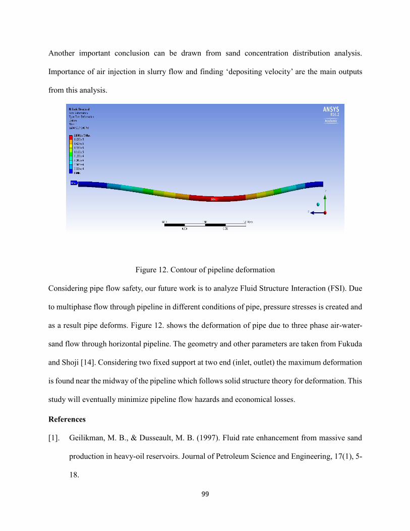
99

Another important conclusion can be drawn from sand concentration distribution analysis.

Importance of air injection in slurry flow and finding ‘depositing velocity’ are the main outputs

from this analysis.

Figure 12. Contour of pipeline deformation

Considering pipe flow safety, our future work is to analyze Fluid Structure Interaction (FSI). Due

to multiphase flow through pipeline in different conditions of pipe, pressure stresses is created and

as a result pipe deforms. Figure 12. shows the deformation of pipe due to three phase air-water-

sand flow through horizontal pipeline. The geometry and other parameters are taken from Fukuda

and Shoji [14]. Considering two fixed support at two end (inlet, outlet) the maximum deformation

is found near the midway of the pipeline which follows solid structure theory for deformation. This

study will eventually minimize pipeline flow hazards and economical losses.

References

[1]. Geilikman, M. B., & Dusseault, M. B. (1997). Fluid rate enhancement from massive sand

production in heavy-oil reservoirs. Journal of Petroleum Science and Engineering, 17(1), 5-

18.

100

[2]. Rajnauth, J., & Barrufet, M. (2012). Monetizing Gas: Focusing on Developments in Gas

Hydrate as a Mode of Transportation. Energy Science and Technology, 4(2), 61-68.

[3]. Xu, H. L., Zhou, G., Wu, B., & Wu, W. R. (2012). Influence of wave and current on deep-

sea mining transporting system. Journal of Central South University, 19, 144-149.

[4]. Miao, Z., Shastri, Y., Grift, T., Hansen, A., & Ting, K. (2012). Lignocellulosic biomass

feedstock transportation alternatives, logistics, equipment configurations, and modeling.

Biofuels, Bioproducts and Biorefining, 6(3), 351-362.

[5]. Bello, O., Reinicke, K., & Teodoriu, C. (2005). Particle Holdup Profiles in Horizontal Gas‐

liquid‐solid Multiphase Flow Pipeline. Chemical Engineering & Technology, 28(12), 1546-

1553.

[6]. Mao, F., Desir, F. K., & Ebadian, M. A. (1997). Pressure drop measurement and correlation

for three-phase flow of simulated nuclear waste in a horizontal pipe. International journal

of multiphase flow, 23(2), 397-402.

[7]. Orell, A. (2007). The effect of gas injection on the hydraulic transport of slurries in

horizontal pipes. Chemical Engineering Science, 62(23), 6659-6676.

[8]. Pouranfard, A. R., Mowla, D., & Esmaeilzadeh, F. (2015). An experimental study of drag

reduction by nanofluids in slug two-phase flow of air and water through horizontal pipes.

Chinese Journal of Chemical Engineering, 23(3), 471-475.

[9]. Sanders, R., Schaan, J., & McKibben, M. (2007). Oil Sand Slurry Conditioning Tests in a

100 mm Pipeline Loop. Canadian Journal of Chemical Engineering, 85(5), 756-764.

[10]. Scott, D. S., & Rao, P. K. (1971). Transport of solids by gas‐liquid mixtures in horizontal

pipes. The Canadian Journal of Chemical Engineering, 49(3), 302-309.

101

[11]. Toda, M., Shimazaki, K., & Maeda, S. (1978). Pressure drop of three-phase flow in

horizontal pipes. Kagaku Kogaku Ronbunshu, 4, 56-62.

[12]. Barnea, D., Shoham, O., Taitel, Y., & Dukler, A. E. (1985). Gas-liquid flow in inclined

tubes: flow pattern transitions for upward flow. Chemical Engineering Science, 40(1), 131-

136.

[13]. Hatate, Y., Nomura, H., Fujita, T., Tajiri, S., & Ikari, A. (1986). Gas holdup and pressure

drop in three-phase horizontal flows of gas-liquid-fine solid particles system. Journal of

chemical engineering of Japan, 19(4), 330-335.

[14]. Fukuda, T., & Shoji, Y. (1986). Pressure Drop and Heat Transfer for Tree Phase Flow: 1st

Report, Flow in Horizontal Pipes. Bulletin of JSME, 29(256), 3421-3426.

[15]. Kago, T., Saruwatari, T., Kashima, M., Morooka, S., & Kato, Y. (1986). Heat transfer in

horizontal plug and slug flow for gas-liquid and gas-slurry systems. Journal of chemical

engineering of Japan, 19(2), 125-131.

[16]. Toda, M., & Konno, H. (1987). Fundamentals of Gas-Liquid-Solid Three Phase Flow.

JAPANESE JOURNAL OF MULTIPHASE FLOW, 1(2), 139-156.

[17]. Angelsen, S., Kvernvold, O., Lingelem, M., & Olsen, S. (1989). Long-Distance Transport

of Unprocess HC Sand Settling in Multiphase Pipelines. In The Fourth International

Conference on Multiphase Flow, Nice, France (pp. 19-21).

[18]. Pieter Oudeman, S. P. E. (1994). Sand Transport and Deposition in Horizontal Multiphase

Trunklines off Subsea Satellite Developments. Transactions, 295, 34.

[19]. Gillies, R. G., McKibben, M. J., & Shook, C. A. (1997). Pipeline flow of gas, liquid and

sand mixtures at low velocities. Journal of Canadian Petroleum Technology, 36(09).

102

[20]. Pironti, F., Pellegrino, G., Meza, G., & Ramírez, N. (1997). Pressure drop of three-phase

suspension flows (water-air-sand) in horizontal pipelines. Revista Técnica de la Facultad de

Ingeniería. Universidad del Zulia, 20(2).

[21]. Salama, M. M. (2000). Sand production management. Journal of energy resources

technology, 122(1), 29-33.

[22]. Stevenson, P., Thorpe, R. B., Kennedy, J. E., & McDermott, C. (2001). The transport of

particles at low loading in near-horizontal pipes by intermittent flow. Chemical Engineering

Science, 56(6), 2149-2159.

[23]. King, M. J., Fairhurst, C. P., & Hill, T. J. (2001). Solids Transport in Multiphase Flows—

Application to High-Viscosity Systems. Journal of energy resources technology, 123(3),

200-204.

[24]. Danielson, T. J. (2007, January). Sand transport modeling in multiphase pipelines. In

Offshore Technology Conference. Offshore Technology Conference.

[25]. Bello, O. O., Udong, I. N., Falcone, G., & Teodoriu, C. (2010, January). Hydraulic analysis

of gas/oil/sand flow in horizontal wells. In SPE Latin American and Caribbean Petroleum

Engineering Conference. Society of Petroleum Engineers.

[26]. Goharzadeh, A., Rodgers, P., & Touati, C. (2010). Influence of Gas-Liquid Two-Phase

Intermittent Flow on Hydraulic Sand Dune Migration in Horizontal Pipelines. Journal of

Fluids Engineering, 132(7), 071301.

[27]. Rahman, M. A., Adane, K. F., & Sanders, R. S. (2013). An improved method for applying

the lockhart–martinelli correlation to three‐phase gas–liquid–solid horizontal pipeline

flows. The Canadian Journal of Chemical Engineering, 91(8), 1372-1382.

103

[28]. Al-Hadhrami, L. M., Shaahid, S. M., Tunde, L. O., & Al-Sarkhi, A. (2014). Experimental

study on the flow regimes and pressure gradients of air-oil-water three-phase flow in

horizontal pipes. The Scientific World Journal,2014.

[29]. Li, L., Xu, H. L., & Yang, F. Q. (2015). Three-phase flow of submarine gas hydrate pipe

transport. Journal of Central South University, 22, 3650-3656.

[30]. Annaland, M., Deen, N. G., & Kuipers, J. A. M. (2005). Numerical simulation of gas–

liquid–solid flows using a combined front tracking and discrete particle method. Chemical

engineering science, 60(22), 6188-6198.

[31]. Washino, Tan, Salman, & Hounslow. (2011). Direct numerical simulation of solid–liquid–

gas three-phase flow: Fluid–solid interaction. Powder Technology, 206(1), 161-169.

[32]. Baltussen, M. W., Seelen, L. J. H., Kuipers, J. A. M., & Deen, N. G. (2013). Direct

Numerical Simulations of gas–liquid–solid three phase flows. Chemical Engineering

Science, 100, 293-299.

[33]. Liu, X., Aramaki, Y., Guo, L., & Morita, K. (2015). Numerical simulation of gas–liquid–

solid three-phase flow using particle methods. Journal of Nuclear Science and Technology,

52(12), 1480-1489.

[34]. Alder, B. J., & Wainwright, T. E. (1960). Studies in molecular dynamics. II. Behavior of a

small number of elastic spheres. The Journal of Chemical Physics, 33(5), 1439-1451.

[35]. Chapman, S., & Cowling, T. G. (1970). The mathematical theory of non-uniform gases: an

account of the kinetic theory of viscosity, thermal conduction and diffusion in gases.

Cambridge university press.

104

[36]. Syamlal, M., Rogers, W., & O’Brien, T. J. (1993). MFIX documentation: Theory guide.

National Energy Technology Laboratory, Department of Energy, Technical Note

DOE/METC-95/1013 and NTIS/DE95000031.

[37]. Vijiapurapu, S., & Cui, J. (2010). Performance of turbulence models for flows through

rough pipes. Applied Mathematical Modelling, 34(6), 1458-1466.

[38]. Zagarola, M. V., & Smits, A. J. (1997). Scaling of the mean velocity profile for turbulent

pipe flow. Physical review letters, 78(2), 239.

[39]. Nourmohammadi, K., Hopke, P. K., & Stukel, J. J. (1985). Turbulent air flow over rough

surfaces: II. turbulent flow parameters. Journal of Fluids Engineering, 107(1), 55-60.

[40]. Kaushal, D. R., Sato, K., Toyota, T., Funatsu, K., & Tomita, Y. (2005). Effect of particle

size distribution on pressure drop and concentration profile in pipeline flow of highly

concentrated slurry. International Journal of Multiphase Flow, 31(7), 809-823.

[41]. Launder, B. E., Reece, G. J., & Rodi, W. (1975). Progress in the development of a Reynolds-

stress turbulence closure. Journal of fluid mechanics, 68(03), 537-566.

[42]. Lien, F. S., & Leschziner, M. A. (1994). Assessment of turbulence-transport models

including non-linear RNG eddy-viscosity formulation and second-moment closure for flow

over a backward-facing step. Computers & Fluids,23(8), 983-1004.

[43]. Daly, B. J., & Harlow, F. H. (1970). Transport equations in turbulence. Physics of Fluids

(1958-1988), 13(11), 2634-2649.

[44]. Launder, B. E. (1989). Second-moment closure: present… and future?. International Journal

of Heat and Fluid Flow, 10(4), 282-300.

105

[45]. Wasp, E. J., Kenny, J. P., & Gandhi, R. L. (1977). Solid--liquid flow: slurry pipeline

transportation. [Pumps, valves, mechanical equipment, economics]. Ser. Bulk Mater. Handl;

(United States), 1(4).

[46]. Brown, N. P., & Heywood, N. I. (Eds.). (1991). Slurry Handling: Design of solid-liquid

systems. Springer Science & Business Media.

[47]. Skudarnov, P., Lin, C., & Ebadian, M. (2004). Double-species slurry flow in a horizontal

pipeline. Journal of Fluids Engineering, Transactions of the ASME, 126(1), 125-132.

[48]. Wood, D. J., 1966, Civil Eng.-A.S.C.E. 36 (12), 60. Cited in Govier, G. W., & Aziz, K.

(1977). The flow of complex mixtures in pipes. Krieger Pub Co.

[49]. Bhagwat, S. M., & Ghajar, A. J. (2016). Experimental investigation of non-boiling gas-

liquid two phase flow in upward inclined pipes. Experimental Thermal and Fluid Science,

79, 301-318.

[50]. Brown, G. O. (2003). The history of the Darcy-Weisbach equation for pipe flow resistance.

In Environmental and Water Resources History (pp. 34-43).

[51]. Colebrook, C. F., Blench, T., Chatley, H., Essex, E., Finniecome, J., Lacey, G., ... &

Macdonald, G. (1939). Correspondence. Turbulent Flow in Pipes, with Particular Reference

to The Transition Region Between the Smooth and Rough Pipe Laws. (Includes Plates).

Journal of the Institution of Civil engineers, 12(8), 393-422.

[52]. Wagner, W., & Kretzschmar, H. J. (2008). IAPWS industrial formulation 1997 for the

thermodynamic properties of water and steam. International Steam Tables: Properties of

Water and Steam Based on the Industrial Formulation IAPWS-IF97, 7-150.

106

Summary

This analysis proposed a multiphase fluid flow model which can be applicable for different

applications specially related to petroleum industry. Our selected model is verified with other

empirical models and available experimental data. It demonstrated very good and acceptable

agreement from single phase to three phase flow. Parametric analysis with two phase and three

phase flow provide some important information about the effects of hydrodynamic parameters on

pressure loss and settling conditions.

Chapter 1 proposed a CFD model with detailed literature analysis and validation of the model with

twelve different experimental sources. Mesh analysis, length independent analysis and turbulent

model selection are done elaborately with several comparisons. As a result, proposed CFD model

showed good agreement with experimental data (maximum error < 30% and average error < 15%).

These indicate validity of our model inside the given ranges.

Chapter 2 tested the effects of fluid flow rate, rotational speed and eccentricity of drill pipe and

solid particle size on pressure loss and settling conditions inside annular pipe using the proposed

CFD model. Preliminary results are presented with proper explanations. Two phase slurry (water

and sand) flow is used to run the parametric analysis changing parameters (fluid velocity, fluid

type, particle size, particle concentration, drill pipe rotation speed and drill pipe eccentricity) inside

annuli. Related two phase flow parametric analysis is represented in Appendix 1 and Appendix 2

using slurry and slug (water and air) flow through pipeline.

Chapter 3 analyzed three phase fluid flow through horizontal pipeline. Air-water-sand flow

through pipeline is used to conduct the analysis changing few major parameters (pipe diameter,

pipe wall roughness, fluid viscosity and sand concentration). Three phase flow analysis is very

107

rare and this preliminary approach in chapter 3 provided the proper guidance for further research.

Related experimental approach with our proposed model is discussed in Appendix 3. Considering

pipe flow safety, Fluid Structure Interaction (FSI) is introduced in this chapter. Because of fluid

flow pressure on wall surface, deformation occurs. This can cause unexpected hazard. FSI analysis

can detect the proper reason of pipe deformations and reduce the risk at work place.

Recommendations for future work:

• Further analysis is required with more accuracy which can include choosing different

coefficients and constants such as coefficient of lift, coefficient of drag, restitution coefficient

and wall boundary conditions to minimize small errors and increase acceptance of this model

at versatile conditions of operation.

• It is expected to find out numerical correlations between different parameters by conducting

further parametric study at distinct phases of fluid flow through pipeline and annuli.

• Complex geometry of pipeline and annuli can be introduced (e.g. bending, inclination etc.).

• Experimental study along with the proposed CFD model will add better scope to study

comprehensively the multiphase flow system through pipeline and annuli. Experimental

facilities are developed in Memorial University of Newfoundland (MUN) and Texas A&M

University at Qatar (TAMUQ) which can be used for further analysis with our findings.

• Elaborate work on Fluid Structure Interaction (FSI) is required focusing the safety and risk of

multiphase flow through pipeline and annuli at different conditions.

108

Appendix 1. Sensitivity Analysis of A CFD Model for Simulating Slurry

Flow Through Pipeline

Rasel A Sultan*, a, M. A. Rahmana, Sohrab Zendehboudia, Vandad Talimib, Vassilios C.

Kelessidisc

aFaculty of Engineering and Applied Science, Memorial University of Newfoundland, St. John’s,

NL, Canada b C-CORE, St. John's, NL, Canada

cFaculty of Petroleum Engineering, Texas A&M University at Qatar, Doha, Qatar

Abstract

Three-dimensional CFD modeling of two-phase slurry flows is shown in this paper through 26mm

diameter horizontal pipe for mixture velocity range of 3.5–4.7m/s and overall volumetric

concentration range of 9.95%–34% with three grain sizes viz. 0.165, 0.29 and 0.55 mm. Eulerian

model with Reynolds Stress Model (RSM) turbulence closure is adopted to analyze the

monodispersed sand particles of varying granular diameters and density 2650 kg/m3. The objective

of this work is to analyze the sensitivity slurry flow using CFD simulation and validating the

simulation with experimental studies available in the literature. The simulated local solid

concentration values and pressure gradients are found to be in good agreement with experimental

results at different conditions. Pressure drop per meter or pressure gradient increases with flow

velocity of mixture. Effects of grain size on various slurry flow parameters especially on local

solid concentration distribution is also studied.

Keywords: CFD; Slurry flow; Pressure gradient; Solid concentration; Pipeline.

Introduction

Liquid-solid and liquid-gas two-phase flow in pipeline or annuli are of great importance in

different industries with transport requirement. In recent years, solid transportation in liquid

109

through pipelines or annuli has become increasingly popular due to its numerous application in

different industries and enormous focus of society on reduction in environmental pollution.

Usually slurry flow has been applied to transport raw materials, wastes and sludges which are in

solid form (Soliman and Collier, 1990), beneficiation in extractive metallurgy and mining plants

(Roco and Shook, 1983), coal processing plants (Choi et al., 2001), fluidized beds (Huilin et al.,

2002), food and chemical plants, petroleum industries and many more. Slurry transportation

system helps to reduce traffic, air pollution, noise, accidents along with saving on energy

consumption and lesser ecological disturbance.

Two-phase slurry flow through pipeline is researched from the beginning of third decade of 20th

century, aiming towards developing general solutions based on available experimental data for

solid volumetric or mass concentration profiles, pressure gradient and slurry velocity profile,

which are primarily required for better understanding of whole slurry flow process. Among the

initial researches, O’Brien (1933) and Rouse (1937) contributed their work of slurry flow in open

channel with low solid concentration, they use diffusion model to predicted the concentration

distribution. Also Durand (1951), Durand and Condolios (1952), Newitt et al. (1955) are

considered as the pioneers to describe friction pressure losses in slurry flow. Correlations

established by Einstein (1906), Thomas (1965) and Krieger (1972) for homogeneous distribution

of slurry and model by Ling et al. (2003) for heterogeneous slurry distribution gave a new

dimension in the study of predicting pressure gradient of slurry flow. Some other works on

empirical correlations for slurry pressure gradient are Govier and Aziz (1972), Vocadlo and

Charles (1972). Aude et al. (1974), Aude et al. (1975), Seshadri (1982) and Seshadri et al. (1982)

studied on long distance slurry flow in pipeline and showed this can be used as a reliable mode of

transportation of solid. Many researches took place aiming at predicting concentration distribution

110

for slurry flow in pipelines. A few notables of them are Shook and Daniel (1965), Shook et al.

(1968), Karabelas (1977), Seshadri et al. (1982), Roco and Shook (1983), Roco and Shook (1984),

Gillies et al. (1991), Gillies and Shook (1994), Gillies et al. (1999), Kaushal and Tomita (2002),

Kaushal and Tomita (2003), Kumar et al. (2003), Kaushal et al. (2005). Apart from this, several

studies for predicting pressure drop over the length also took place for slurry flows. A few notables

of them are Wasp et al. (1970), Wilson (1976), Wasp et al. (1977), Doron et al. (1987), Gillies et

al. (1991), Sundqvist et al. (1996), Mishra et al. (1998), Ghanta and Purohit (1999), Wilson et al.

(2002), Kaushal and Tomita (2002), Kumar (2002), Kaushal and Tomita (2003), Skudarnov et al.

(2004), Kaushal et al. (2005), Kumar et al. (2008), Vlasak et al. (2012), Pouranfard (2014). These

empirical correlations and experimental studies are based on limited scope, data and application

range (Lahiri and Ghanta, 2007). CFD simulation models have been utilized to minimize these

limitations. CFD studies by Hernández et al. (2008), Chen et al. (2009), Kumar and Kaushal

(2015), Kumar and Kaushal (2016) on slurry flow in pipeline have provided a new dimension in

this field.

The approach of this study is to perform several comparisons of CFD simulation with experimental

and empirical studies at different conditions and ranges for different industrial purposes. A

parametric study is conducted using CFD simulation with versatile range of variables to minimize

limitation in applications. Furthermore, different variables like modelling pressure loss,

measuring/modeling concentration profile, analyzing the physics that control the hydrodynamics

of fluid flow in annuli or pipeline is studied.

Mathematical Models

The Eulerian model of granular version has been adopted as multiphase model for present study.

The selection of appropriate multiphase model depends mainly on the range of volume fraction

111

(α) of solid phase under consideration. Since high value of volume fraction is used in this study

this model is taken into account. Granular version helps in capturing the effects of friction and

collusions between particles which is especially important in higher concentration slurries having

varying grain sizes.

Multiphase Model

The Eulerian multiphase model allows for the modeling of multiple separate, yet interacting

phases. The phases can be liquids, gases, or solids in nearly any combination. The Eulerian

treatment is used for each phase, in contrast to the Eulerian-Lagrangian treatment that is used for

the discrete phase model.

Volume Fractions


volume fractions, denoted here by 𝑎𝑞. Volume fractions represent the space occupied by each

phase, and the laws of conservation of mass and momentum are satisfied by each phase

individually. The derivation of the conservation equations can be done by ensemble averaging the

local instantaneous balance for each of the phases (Anderson and Jackson, 1967) or by using the

mixture theory approach (Bowen, 1976).

The volume of phase 𝑞, 𝑉𝑞, is defined by


where,

∑ 𝑎𝑞 = 1𝑛𝑞=1 (2)

112

The effective density of phase 𝑞 is,

𝑞 = 𝑎𝑞𝜌𝑞 (3)

where 𝜌𝑞 is the physical density of phase 𝑞.

Conservation Equations

The equations for fluid-fluid and granular multiphase flows, are presented here for the general case

of an 𝑛 -phase flow.

Continuity Equation

The volume fraction of each phase is calculated from a continuity equation as below –

1

𝜌𝑟𝑞𝜕

𝜕𝑡(𝑎𝑞𝜌𝑞) + ∇. (𝑎𝑞𝜌𝑞𝜗𝑞 ) = ∑ (𝑝𝑞 − 𝑞𝑝)

𝑛𝑝=1 (4)

where 𝜌𝑟𝑞 is the phase reference density, or the volume averaged density of the 𝑞𝑡ℎ phase in the

solution domain, 𝑝𝑞 characterizes the mass transfer from the 𝑝𝑡ℎ to 𝑞𝑡ℎ phase and

𝑞𝑝 characterizes the mass transfer from the 𝑞𝑡ℎ to 𝑝𝑡ℎ phase.

Fluid-Fluid Momentum Equations

The conservation of momentum for a fluid phase 𝑞 is –

𝜕


𝑛𝑝=1


Here 𝑔 is the acceleration due to gravity, 𝜏 is the 𝑞𝑡ℎ phase stress-strain tensor, 𝐹𝑞 is an external


113

Fluid-Solid Momentum Equations

Following the work of Alder and Wainwrigh (1960), Chapman and Cowling (1970) and Syamlal

et al. (1993), a multi-fluid granular model is used to describe the flow behavior of a fluid-solid

mixture.

The conservation of momentum for the fluid phases is similar to Equation (5), and that for the 𝑠𝑡ℎ

solid phase is –

𝜕


𝑁𝑙=1


where 𝑝𝑠 is the 𝑠𝑡ℎ solids pressure, 𝐾𝑙𝑠 = 𝐾𝑠𝑙 is the momentum exchange coefficient between


Solids Pressure

For granular flows in the compressible regime (i.e., where the solids volume fraction is less than

its maximum allowed value), a solids pressure is calculated independently and used for the

pressure gradient term, ∇𝑝𝑠 in the granular-phase momentum equation. Because a Maxwellian

velocity distribution is used for the particles, a granular temperature is introduced into the model,

and appears in the expression for the solids pressure and viscosities. The solids pressure is

composed of a kinetic term and a second term due to particle collisions –


where, 𝑒𝑠𝑠 is the coefficient of restitution for particle collisions, 𝑔0,𝑠𝑠 is the radial distribution

function, and 𝛩𝑠 is the granular temperature. Here a default value of 0.9 for 𝑒𝑠𝑠 is used, but the

114

value can be adjusted to suit the particle type. The granular temperature 𝛩𝑠 is proportional to the

kinetic energy of the fluctuating particle motion. The function 𝑔0,𝑠𝑠 is a distribution function that

governs the transition from the "compressible'' condition with 𝑎 < 𝑎𝑠,𝑚𝑎𝑥, where the spacing

between the solid particles can continue to decrease, to the "incompressible'' condition with 𝑎 =

𝑎𝑠,𝑚𝑎𝑥, where no further decrease in the spacing can occur. A value of 0.63 is the default

for 𝑎𝑠,𝑚𝑎𝑥, but it can be modify during the problem setup.

Solids Shear Stresses

The solids stress tensor contains shear and bulk viscosities arising from particle momentum

exchange due to translation and collision. A frictional component of viscosity can also be included

to account for the viscous-plastic transition that occurs when particles of a solid phase reach the

maximum solid volume fraction.

The collisional and kinetic parts, and the optional frictional part, are added to give the solids shear

viscosity-


where, 𝜇𝑠,𝑐𝑜𝑙 is shear viscosity due to collision, 𝜇𝑠,𝑘𝑖𝑛 is kinetic viscosity and 𝜇𝑠,𝑓𝑟 frictional

viscosity.

The collisional part of the shear viscosity is modeled as Gidaspow et al. (1991) and Syamlal et al.

(1993) –

𝜇𝑠,𝑐𝑜𝑙 = 4

5𝑎𝑠𝜌𝑠𝑑𝑠𝑔0,𝑠𝑠(1 + 𝑒𝑠𝑠) (

𝛩𝑠

𝜋)1/2

(9)

The default expression of kinetic viscosity is from Syamlal et al. (1993):

115

𝜇𝑠,𝑘𝑖𝑛 = 𝑎𝑠𝑑𝑠𝜌𝑠√𝛩𝑠𝜋

6(3− 𝑒𝑠𝑠)[1 +

2

5(1 + 𝑒𝑠𝑠)(3𝑒𝑠𝑠 − 1)𝑎𝑠𝑔0,𝑠𝑠] (10)

The frictional viscosity is included using Schaeffer’s (1987) expression –

𝜇𝑠,𝑓𝑟 = 𝑝𝑠 sin∅

2√𝐼2𝐷 (11)

Turbulence Model

Turbulent quantity for fluid flow are assumed using Reynolds Stress Model (RSM) (Launder et

al., 1975, Gibson and Launder, 1978 and Launder, 1989). This is the most elaborate turbulence

model. Abandoning the isotropic eddy-viscosity hypothesis, the RSM closes the Reynolds-

averaged Navier-Stokes equations (Chorin, 1968) by solving transport equations for the Reynolds

stresses, together with an equation for the dissipation rate. Here five additional transport equations

are required in 2D flows and seven additional transport equations must be solved in 3D.

The exact transport equation for the Reynolds Stress Model (RSM) is as below –

𝜕

𝜕𝑡(𝜌𝑢𝑖′𝑢𝑗′ )

⏟ 𝐿𝑜𝑐𝑎𝑙 𝑇𝑖𝑚𝑒 𝐷𝑒𝑟𝑖𝑣𝑎𝑡𝑖𝑣𝑒

+ 𝜕

𝜕𝑥𝑘(𝜌𝑢𝑘𝑢𝑖′𝑢𝑗′ )

⏟ 𝐶𝑜𝑛𝑣𝑒𝑐𝑡𝑖𝑜𝑛 (𝐶𝑖𝑗)

= −𝜕

𝜕𝑥𝑘[𝜌𝑢𝑖′𝑢𝑗′𝑢𝑘

′ + 𝑝 (𝛿𝑘𝑗𝑢𝑖′ + 𝛿𝑖𝑘𝑢𝑗′) ]

⏟ 𝑇𝑢𝑟𝑏𝑢𝑙𝑒𝑛𝑡 𝐷𝑖𝑓𝑓𝑢𝑠𝑖𝑜𝑛 (𝐷𝑇,𝑖𝑗)

+ 𝜕

𝜕𝑥𝑘[𝑢𝜕𝑦

𝜕𝑥𝑘(𝑢𝑖′𝑢𝑗′ )]

⏟ 𝑀𝑜𝑙𝑒𝑐𝑢𝑙𝑎𝑟 𝐷𝑖𝑓𝑓𝑢𝑠𝑖𝑜𝑛 (𝐷𝐿,𝑖𝑗)

− 𝜌 (𝑢𝑖′𝑢𝑘′ 𝜕𝑢𝑗

𝜕𝑥𝑘+ 𝑢𝑗′𝑢𝑘

′ 𝜕𝑢𝑗

𝜕𝑥𝑘)

⏟ 𝑆𝑡𝑟𝑒𝑠𝑠 𝑃𝑟𝑜𝑢𝑐𝑡𝑖𝑜𝑛 (𝑃𝑖𝑗)

− 𝜌𝛽(𝑔𝑖𝑢𝑗′𝜃 + 𝑔𝑖𝑢𝑖′𝜃)⏟ 𝐵𝑢𝑜𝑦𝑎𝑛𝑐𝑦 𝑃𝑟𝑜𝑑𝑢𝑐𝑡𝑖𝑜𝑛 (𝐺𝑖𝑗)

+ 𝑝 (𝜕𝑢𝑖

′

𝜕𝑥𝑗+𝜕𝑢𝑗

′

𝜕𝑥𝑖)

⏟ 𝑃𝑟𝑒𝑠𝑠𝑢𝑟𝑒 𝑆𝑡𝑟𝑎𝑖𝑛 (∅𝑖𝑗)

− 2𝜇

𝜕𝑢𝑖′

𝜕𝑥𝑘

𝜕𝑢𝑗′

𝜕𝑥𝑘

⏟ 𝐷𝑖𝑠𝑠𝑖𝑝𝑎𝑡𝑖𝑜𝑛 (𝜖𝑖𝑗)

(12)

−2𝜌𝛺𝑘(𝑢𝑗′𝑢𝑚′ 𝜖𝑖𝑘𝑚 + 𝑢𝑖′𝑢𝑚′ 𝜖𝑗𝑘𝑚)⏟ 𝑃𝑟𝑜𝑑𝑢𝑐𝑡𝑖𝑜𝑛 𝑏𝑦 𝑠𝑦𝑠𝑡𝑒𝑚 𝑅𝑜𝑡𝑎𝑡𝑖𝑜𝑛 (𝐹𝑖𝑗)

+ 𝑆𝑢𝑠𝑒𝑟⏟𝑈𝑠𝑒𝑟−𝐷𝑒𝑓𝑖𝑛𝑒𝑑 𝑆𝑜𝑢𝑟𝑐𝑒

116

Of the various terms in these exact equations, 𝐶𝑖𝑗, 𝐷𝐿,𝑖𝑗, 𝑃𝑖𝑗 and 𝐹𝑖𝑗 do not require any modeling.

However, 𝐷𝑇,𝑖𝑗, 𝐺𝑖𝑗, ∅𝑖𝑗 and 𝜖𝑖𝑗 need to be modeled to close the equations 𝐷𝑇,𝑖𝑗 can be modeled

by the generalized gradient-diffusion model of Daly and Harlow (1970), which is –

𝐷𝑇,𝑖𝑗 = 𝐶𝑠𝜕

𝜕𝑥𝑘(𝜌

𝑘𝑢𝑘′ 𝑢𝑖

′

𝜖

𝜕𝑢𝑖′𝑢𝑗′

𝜕𝑥𝑙) (13)

However, this equation can result in numerical instabilities (Launder, 1989), so it has been

simplified in this study to use a scalar turbulent diffusivity as follows (Launder, 1989) –



𝜎𝑘


𝜕𝑥𝑘) (14)

Lien and Leschziner (Lien and Leschziner, 1987) derived a value of adjustable constant 𝜎𝑘 = 0.82.

where, turbulent viscosity (𝜇𝑡) is computed as –

𝜇𝑡 = 𝜌𝐶𝜇𝑘2

𝜖 𝑎𝑛𝑑 𝐶𝜇 = 0.09 (15)

where, 𝐶𝜇 is an adjustable constant.

Expression for 𝐺𝑖𝑗 for ideal gases is as follows –

𝐺𝑖𝑗 = −𝜇𝑡

𝜌𝑃𝑟𝑡(𝑔𝑖

𝜕𝜌

𝜕𝑥𝑗+ 𝑔𝑗

𝜕𝜌

𝜕𝑥𝑖) (16)

where 𝑃𝑟𝑡 is the turbulent Prandtl number for energy, with a default value of 0.85 used in

simulation.

The pressure-strain term, ∅𝑖𝑗 is modeled according to the proposal by Gibson and Launder (1978),

Fu et al. (1987), and Launder (1989).

The classical approach to modeling ∅𝑖𝑗 uses the following decomposition –

117

∅𝑖𝑗 = ∅𝑖𝑗,1 + ∅𝑖𝑗,2 + ∅𝑖𝑗,𝑤 (17)

where, ∅𝑖𝑗,1is the slow pressure-strain term, also known as the return-to-isotropy term, ∅𝑖𝑗,2 is

called the rapid pressure-strain term, and ∅𝑖𝑗,𝑤 is the wall-reflection term.

The slow pressure-strain term, ∅𝑖𝑗,1, is modeled as -

∅𝑖𝑗,1 ≡ −𝐶1𝜌𝜖


2

3𝛿𝑖𝑗𝑘] (18)

with, 𝐶1 = 1.8.

The rapid pressure-strain term, ∅𝑖𝑗,2, is modeled as –

∅𝑖𝑗,2 ≡ 𝐶2 [(𝑃𝑖𝑗 + 𝐹𝑖𝑗 + 𝐺𝑖𝑗 − 𝐶𝑖𝑗) − 2

3𝛿𝑖𝑗(𝑃 + 𝐺 − 𝐶)] (19)

where 𝐶2 = 0.60, 𝑃𝑖𝑗, 𝐹𝑖𝑗, 𝐺𝑖𝑗 and 𝐶𝑖𝑗 are defined as in Equation (12), 𝑃 = 1

2𝑃𝑘𝑘, 𝐺 =

1

2𝐺𝑘𝑘, 𝐶 =

1

2𝐶𝑘𝑘.

The wall-reflection term, ∅𝑖𝑗,𝑤 is responsible for the redistribution of normal stresses near the wall.

It tends to damp the normal stress perpendicular to the wall, while enhancing the stresses parallel

to the wall. This term is modeled as –

∅𝑖𝑗,𝑤 ≡ 𝐶1′𝜖

𝑘(𝑢𝑘

′ 𝑢𝑚′ 𝑛𝑘𝑛𝑚𝛿𝑖𝑗 − 3

2𝑢𝑖′𝑢𝑘

′ 𝑛𝑗𝑛𝑘 − 3

2𝑢𝑗′𝑢𝑘

′ 𝑛𝑖𝑛𝑘)𝐶𝑙𝑘

32

𝜖𝑑

+ 𝐶2′ (∅𝑘𝑚,2𝑛𝑘𝑛𝑚𝛿𝑖𝑗 −

3

2∅𝑖𝑘,2𝑛𝑗𝑛𝑘 −

3

2∅𝑗𝑘,2𝑛𝑖𝑛𝑘)

𝐶𝑙𝑘32

𝜖𝑑 (20)

118

where 𝐶1′ = 0.5, 𝐶2

′ = 0.3, 𝑛𝑘 is the 𝑥𝑘 component of the unit normal to the wall, 𝑑 is the normal

distance to the wall, and 𝐶𝑙 = 𝐶𝜇

34

𝑘, where 𝐶𝜇 = 0.09 and 𝑘 is the von Kármán constant (= 0.4187)

(Karman, 1937).

The dissipation tensor, 𝜖𝑖𝑗, is modeled as –

𝜖𝑖𝑗 = 2

3𝛿𝑖𝑗(𝜌𝜖 + 𝑌𝑀) (21)

where 𝑌𝑀 = 2𝜌𝜖𝑀𝑡2 is an additional "dilatation dissipation'' term according to the model by Sarkar

(1991). The turbulent Mach number in this term is defined as –

𝑀𝑡 = √𝑘

𝑎2 (22)

Solution Method

For Eulerian multiphase calculations, the phase coupled SIMPLE (PC-SIMPLE) algorithm

(Vasquez and Ivanov, 2000) is used for the pressure-velocity coupling. PC-SIMPLE is an

extension of the SIMPLE algorithm (Patankar, 1980) to multiphase flows. The velocities are

solved coupled by phases, but in a segregated fashion. The block algebraic multigrid scheme used

by the density-based solver described in (Weiss et al., 1999) is used to solve a vector equation

formed by the velocity components of all phases simultaneously. Then, a pressure correction

equation is built based on total volume continuity rather than mass continuity. Pressure and

velocities are then corrected so as to satisfy the continuity constraint.

Pressure-Correction Equation

For incompressible multiphase flow, the pressure-correction equation takes the form of –

119

∑1

𝜌𝑟𝑘

𝑛𝑘=1

𝜕

𝜕𝑡𝑎𝑘𝜌𝑘 + ∇. 𝑎𝑘𝜌𝑘𝑣 𝑘

′ + ∇. 𝑎𝑘𝜌𝑘𝑣 𝑘∗ − (∑ (𝑙𝑘 − 𝑘𝑙)

𝑛𝑙=1 ) = 0 (23)

where 𝜌𝑟𝑘 is the phase reference density for the 𝑘𝑡ℎ phase (defined as the total volume average

density of phase 𝑘), 𝑣 𝑘′ is the velocity correction for the 𝑘𝑡ℎ phase, and 𝑣 𝑘

∗ is the value of 𝑣 𝑘 at the

current iteration.

Volume Fractions

The volume fractions are obtained from the phase continuity equations. In discretized form, the

equation of the 𝑘𝑡ℎ volume fraction is –

𝑎𝑝,𝑘𝑎𝑘 = ∑ (𝑎𝑛𝑏,𝑘𝑎𝑛𝑏,𝑘) + 𝑏𝑘 = 𝑅𝑘𝑛𝑏 (24)

In order to satisfy the condition that all the volume fractions sum to one,

∑ 𝑎𝑘 = 1𝑛𝑘=1 (25)


Geometry and mesh generation

In the present study, a 13.15m long and 26.0mm internal diameter pipe is selected for the

sensitivity analysis. The computational grids for this horizontal pipe is generated using ANSYS

Fluent meshing with 1,86,767 elements with 82,827 nodes volume cells finalized conducting

proper mesh independency check. Ten layers of Inflation near wall is added to observe more

preciously the characteristics of different parameters near wall. Shear stress between wall surface

and gas molecules are much higher and this inflation helps to create denser meshing near wall.

Also it is more time consuming and reliable to use unsymmetrical meshing rather symmetrical

meshing. The length of the pipe is sufficient enough to achieve a fully developed

120

Fig.1. Mesh distribution in the pipe geometry

flow at the outlet as minimum flow development section should be at least 50D (D = internal

diameter of pipe) (Wasp et al., 1977, Brown and Heywood, 1991) and here this length is

maintained. Comutational grid distribution of geometry is shown in Figure 1.

Boundary conditions

There are three boundaries available in the given flow domain namely the inlet boundary, the wall

boundary and the outlet boundary. Here, inlet velocity range of 3.5–4.7m/s and overall volumetric

concentration range of 9%–34% with three grain sizes viz. 0.165, 0.29 and 0.55 mm have been

considered as boundary input. A 0.2 mm of pipe wall roughness is adopted during simulation. As

the nature of wall-particle collisions influences the shear stress and turbulent energy flux at the

walls, a specularity coefficient is defined for solid phase at the walls. a value of 0.5 is selected

which corresponds to wall quality between smooth frictionless walls and very rough walls. No slip

for liquid phase has been adopted at walls. Inlet and outlet pressure are assumed same.

121

Solution process and convergence criteria

Fluent, ver. 16.2, ANSYS Inc. is used to build a CFD simulation model of pipeline flow of water-

sand slurry. A convergence value of 10-5 has been adopted for termination of iteration, this value

is slelected with optimizing analysis to have most satisfactory accuracy with less time. A second

order upwind discretization for momentum equation and first upwind discretization for volume

fraction, turbulent kinetic energy and its dissipation are adopted to ensure stability and

convergence of iterative process.

Validation of Simulation

Comparison of pressure gradient

Pressure gradient of water-sand slurry flow from simulation is compared with Skudarnov et al.

(2004) experimental data. In the experiment, length of pipe is 17m, diameter of pipe is 0.023m,

fluid taken water (density 9982 Kg/m3, viscosity 0.001003 Kg/m-s) and slurry taken glass spheres

slurry (double-species slurry with densities of 2490 kg/m3 and 4200 kg/m3, 50% by 50% by

volume mixtures), wall material is stainless steel (density 8030 kg/m3, roughness 32 µm). Figure

2 shows the comparison of pressure gradient with dm = 140 µm and Cv = 15%. Where, dm = mean

particle diameter (µm) Cv = volume concentration (%).

122

Fig.2. Comparison of pressure gradient from simulation with experimental data of Skudarnov

et al. (2004) for double-species slurry with dm = 140 µm and Cv = 15%.

The result shows very good aggrement with experiemntal values with less than 10% error at each

point. The small errors that are arising may be due to experimental errors (it was estimated in the

reference paper that the accuracy of the pressure gradient is ±50 Pa/m.) and numerical error of

mathematical equations while applying simulation.

Comparison of local solid concentration profile

Local solid concentration profile of water-sand slurry flow from simulation is compared with

Gillies and Shook, (1994) experimental data. In the experiment, length of pipe is 2.7m, diameter

of pipe is 53.2mm, fluid taken water (density 9982 Kg/m3, viscosity 0.001003 Kg/m-s) and slurry

taken Silica (chemical formula SiO2, density 2650 Kg/m3, wall material is aluminum (density 2800

kg/m3, roughness 0.2mm). Here, grain size or mean partical diameter is 0.18 mm, mixture velocity

3.1 m/s and three different solid volumetric concentration 14%, 29% and 45% is considered from

experiment. Figure 3 shows the comparison of volumetric concentration of solid particles with

particle sizes 0.18 mm.

0

2000

4000

6000

8000

1 1.2 1.4 1.6 1.8 2 2.2 2.4Pre

ssure

Gra

die

nt

(Pa/

m)

Flow Velocity (m/s)

Experiment (Skudarnov

et al., 2004)

Simulation

123

Fig. 3. Comparison of simulated and measured values of local volumetric concentration of solid

across vertical centerline for particle sizes 0.18 mm.

Simulated results are in good agreement with experimental values for grain sizes 0.18mm.

However, simulated values deviate from experimental values near the wall especially in the lower

half of the cross-section. One of the possible reasons could be abrasive rounding of these large size

particles by repeated passages during experiment, resulting significant quantities of fines were

generated which were distributed uniformly within the pipe. This would have led to possible

increase in carrier density. Since information of this aspect was not available in the reference

research, the same is not incorporated while doing simulations.

-1

-0.5

0

0.5

1

0 0.2 0.4 0.6

Y/R


Simulation (14% Vol

Concentration)

Simulation (29% Vol

Concentration)

Simulation (45% Vol

Concentration)

Experiment (14% Vol

Concentration)

Experiment (29% Vol

Concentration)

Experiment (45% Vol

Concentration)

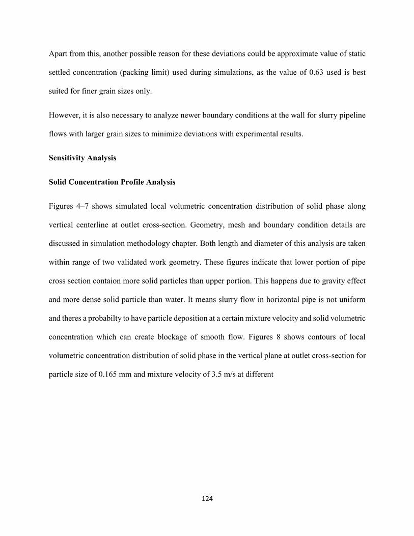
124

Apart from this, another possible reason for these deviations could be approximate value of static

settled concentration (packing limit) used during simulations, as the value of 0.63 used is best

suited for finer grain sizes only.

However, it is also necessary to analyze newer boundary conditions at the wall for slurry pipeline

flows with larger grain sizes to minimize deviations with experimental results.

Sensitivity Analysis

Solid Concentration Profile Analysis

Figures 4–7 shows simulated local volumetric concentration distribution of solid phase along

vertical centerline at outlet cross-section. Geometry, mesh and boundary condition details are

discussed in simulation methodology chapter. Both length and diameter of this analysis are taken

within range of two validated work geometry. These figures indicate that lower portion of pipe

cross section contaion more solid particles than upper portion. This happens due to gravity effect

and more dense solid particle than water. It means slurry flow in horizontal pipe is not uniform

and theres a probabilty to have particle deposition at a certain mixture velocity and solid volumetric

concentration which can create blockage of smooth flow. Figures 8 shows contours of local

volumetric concentration distribution of solid phase in the vertical plane at outlet cross-section for

particle size of 0.165 mm and mixture velocity of 3.5 m/s at different

125

Fig.4. Simulated local volumetric sand concentration across vertical centre line of pipe outlet for

particle size of 0.165 mm and mixture velocity of 3.5 m/s at different efflux concentrations.

-1.5

-1

-0.5

0

0.5

1

1.5

0 0.2 0.4 0.6

Y/R

Sand Concentration

Pipe Diameter = 26 mm & Particle Size = 0.165 mm

Mixture Velocity = 3.5 m/s

Simulation (9.95% vol

concentration)


concentration)


concentration)


concentration)

126



-1.5

-1

-0.5

0

0.5

1

1.5

0 0.2 0.4 0.6 0.8

Y/R

Sand Concentration




concentration)


concentration)


concentration)

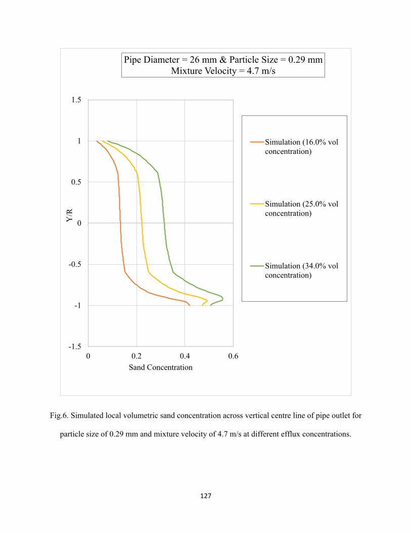
127



-1.5

-1

-0.5

0

0.5

1

1.5

0 0.2 0.4 0.6

Y/R

Sand Concentration




concentration)


concentration)


concentration)

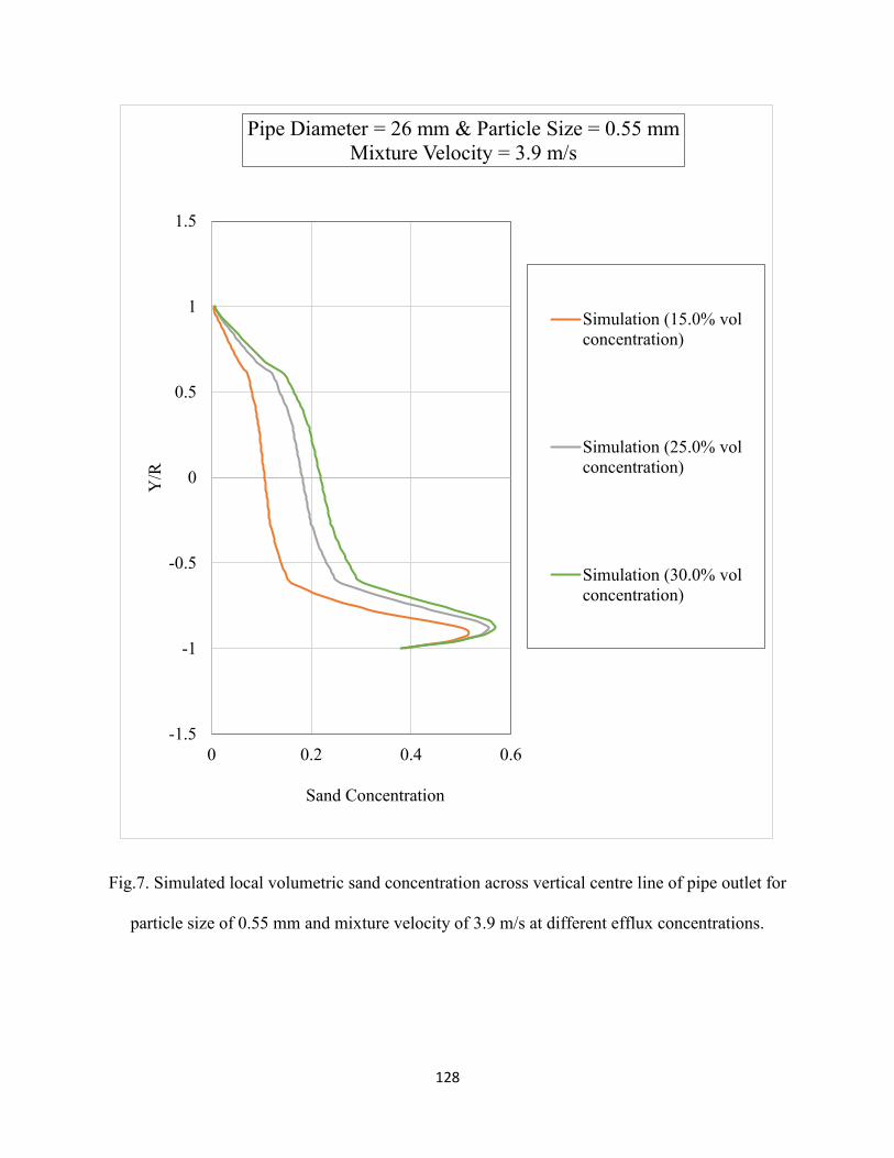
128



-1.5

-1

-0.5

0

0.5

1

1.5

0 0.2 0.4 0.6

Y/R

Sand Concentration




concentration)


concentration)


concentration)

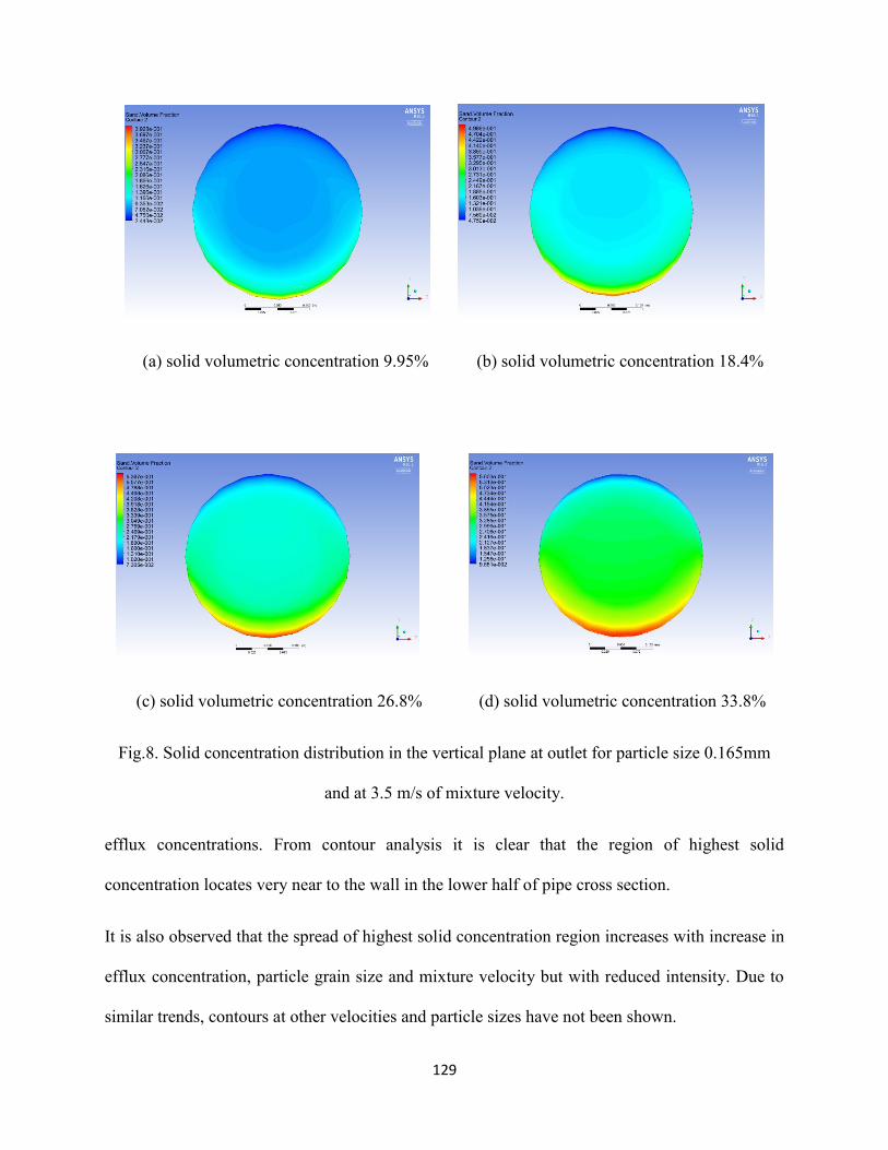
129

(a) solid volumetric concentration 9.95% (b) solid volumetric concentration 18.4%

(c) solid volumetric concentration 26.8% (d) solid volumetric concentration 33.8%

Fig.8. Solid concentration distribution in the vertical plane at outlet for particle size 0.165mm

and at 3.5 m/s of mixture velocity.

efflux concentrations. From contour analysis it is clear that the region of highest solid

concentration locates very near to the wall in the lower half of pipe cross section.

It is also observed that the spread of highest solid concentration region increases with increase in

efflux concentration, particle grain size and mixture velocity but with reduced intensity. Due to

similar trends, contours at other velocities and particle sizes have not been shown.

130

Conclusion

Keeping in mind to develope a widely accepted, reliable, efficient CFD model this paper analyze

CFD simulation of two phase (sand-water) slurry flows through 26 mm diameter pipe in horizontal

orientation for flow velocity range of 3.5-4.7 m/s and efflux concentration range of 9.95-34% with

three particle sizes viz. 0.165 mm, 0.29 mm and 0.55 mm with density 2650 kg/m3. Local

volumetric concentration of solid particle at pipe outlet is very well simulated for different

combinations of particle size, mixture velocity and efflux concentrations under consideration.

Before these analysis, this simulation model is validated with two different experimental results

having different boundary conditions from available literatures. This comparison process shows

very good aggrement with experimental result and validate our model over certain range of

operating condition. Mathematical equations of multiphase flow and turbulence models is also

added to explain our simulation process with its acceptancy at certain operating conditions.

This study helps to understand two phase slurry flows for different applications. The analysis of

local solid concentration can give idea of selecting optimizing range of particle size, volumetric

concentration of slurry and mixture velocity during operation. This study can lead to find out

‘deposition velocity’ in slurry flow. However, scatter in simulation data of various flow parameters

especially with bigger particle sizes of slurry indicates that the model used in the present study

needs further development. Also it can be seen from figures 3, 6 and 7 that sudden reduction of

solid concentration is occuring near wall with higher efflux concentration and particle size, which

is not expected practically. This indicates simulation instability near lower wall over a range of

efflux concentration and particle size, this needs to be solved. The choice of different coefficients

and constants such as coefficient of lift, coefficient of drag, restitution coefficient and wall

131

boundary conditions needs to be further researched. Also introducing three phase flow adding gas

can lead to new findings and benifits with this two phase slurry flow.

References

Alder, B. J., & Wainwright, T. E. (1960). Studies in molecular dynamics. II. Behavior of a small

number of elastic spheres. The Journal of Chemical Physics, 33(5), 1439-1451.

Anderson, T. B., & Jackson, R. (1967). Fluid mechanical description of fluidized beds. Equations

of motion. Industrial & Engineering Chemistry Fundamentals, 6(4), 527-539.

Aude, T. C., Thompson, T. L., & Wasp, E. J. (1974). Economics of slurry pipeline

systems. Publication of: Cross (Richard B) Company, 15(Proc Paper).

Aude, T. C., Thompson, T. L., & Wasp, E. J. (1975). Slurry-pipeline systems for coal; other solids

come of age. Oil Gas J.; (United States), 73(29).

Bowen, R. M. (1976). Theory of mixtures. Continuum physics, 3(Pt I).

Brown, N. P., & Heywood, N. I. (Eds.). (1991). Slurry Handling: Design of solid-liquid systems.

Springer Science & Business Media.

Chapman, S., & Cowling, T. G. (1970). The mathematical theory of non-uniform gases: an

account of the kinetic theory of viscosity, thermal conduction and diffusion in gases.

Cambridge university press.

Chen, L., Duan, Y., Pu, W., & Zhao, C. (2009). CFD simulation of coal-water slurry flowing in

horizontal pipelines. Korean journal of chemical engineering, 26(4), 1144-1154.

Choi, Young-Chan, Park, Tae-Jun, Kim, Jae-Ho, Lee, Jae-Goo, Hong, Jae-Chang, & Kim, Yong-

Goo. (2001). Experimental studies of 1 ton/day coal slurry feed type oxygen blown, entrained

flow gasifier. Korean Journal of Chemical Engineering, 18(4), 493-498.

132

Chorin, A. J. (1968). Numerical solution of the Navier-Stokes equations. Mathematics of

computation, 22(104), 745-762.

Daly, B. J., & Harlow, F. H. (1970). Transport equations in turbulence. Physics of Fluids (1958-

1988), 13(11), 2634-2649.

Doron, P., Granica, D., & Barnea, D. (1987). Slurry flow in horizontal pipes—experimental and

modeling. International Journal of Multiphase Flow, 13(4), 535-547.

Durand, R. (1951). Transport hydraulique de graviers et galets en conduite. La Houille Blanche,

609-619.

Durand, R., & Condolios, E. (1952, November). The hydraulic transport of coal and solid material

in pipes. In Proceedings of Colloquium on Hydraulic Transportation, France.

Durand, R., & Condolios, E. (1952). Experimental study on conveying solids in pipes, 2 emes

journees de l'hydraaulique. Soc. Hydrotech. Fr, 29.

Einstein, A. (1906). Zur theorie der brownschen bewegung. Annalen der physik, 324(2), 371-381.

Fu, S., Launder, B. E., & Leschziner, M. A. (1987). Modelling strongly swirling recirculating jet

flow with Reynolds-stress transport closures. In 6th Symposium on Turbulent Shear Flows (pp.

17-6).

Ghanta, K. C., & Purohit, N. K. (1999). Pressure drop prediction in hydraulic transport of bi-

dispersed particles of coal and copper ore in pipeline. The Canadian Journal of Chemical

Engineering, 77(1), 127-131.

Gibson, M. M., & Launder, B. E. (1978). Ground effects on pressure fluctuations in the

atmospheric boundary layer. Journal of Fluid Mechanics,86(03), 491-511.

133

Gidaspow, D., Bezburuah, R., & Ding, J. (1991). Hydrodynamics of circulating fluidized beds:

kinetic theory approach (No. CONF-920502-1). Illinois Inst. of Tech., Chicago, IL (United

States). Dept. of Chemical Engineering.

Gillies, R. G., Shook, C. A., & Wilson, K. C. (1991). An improved two layer model for horizontal

slurry pipeline flow. The Canadian Journal of Chemical Engineering, 69(1), 173-178.

Gillies, R. G., & Shook, C. A. (1994). Concentration distributions of sand slurries in horizontal

pipe flow. Particulate science and technology, 12(1), 45-69.

Gillies, R. G., Hill, K. B., Mckibben, M. J., & Shook, C. A. (1999). Solids transport by laminar

Newtonian flows. Powder Technology, 104(3), 269-277.

Gopaliya, M. K., & Kaushal, D. R. (2015). Analysis of Effect of Grain Size on Various Parameters

of Slurry Flow through Pipeline Using CFD.Particulate Science and Technology, 33(4), 369-

384.

Govier, G., & Aziz, K. (1972). The flow of complex mixtures in pipes. New York: Van Nostrand

Reinhold.

Hernández, F. H., Blanco, A. J., & Rojas-Solórzano, L. (2008, January). CFD modeling of slurry

flows in horizontal pipes. In ASME 2008 Fluids Engineering Division Summer Meeting

collocated with the Heat Transfer, Energy Sustainability, and 3rd Energy Nanotechnology

Conferences (pp. 857-863). American Society of Mechanical Engineers.

Huilin, Gidaspow, & Bouillard. (2002). Chaotic behavior of local temperature fluctuations in a

laboratory-scale circulating fluidized bed. Powder Technology, 123(1), 59-68.

Karabelas, A. J. (1977). Vertical distribution of dilute suspensions in turbulent pipe flow. AIChE

Journal, 23(4), 426-434.

134

Karman, T. V. (1937). The fundamentals of the statistical theory of turbulence. Journal of the

Aeronautical Sciences, 4(4), 131-138.

Kaushal, D. R., & Tomita, Y. (2002). Solids concentration profiles and pressure drop in pipeline

flow of multisized particulate slurries. International journal of multiphase flow, 28(10), 1697-

1717.

Kaushal, D. R., & Tomita, Y. (2003). Comparative study of pressure drop in multisized particulate

slurry flow through pipe and rectangular duct. International Journal of Multiphase

Flow, 29(9), 1473-1487.

Kaushal, D. R., Sato, K., Toyota, T., Funatsu, K., & Tomita, Y. (2005). Effect of particle size

distribution on pressure drop and concentration profile in pipeline flow of highly concentrated

slurry. International Journal of Multiphase Flow, 31(7), 809-823.Krieger, I. M. (1972).

Rheology of monodisperse latices. Advances in Colloid and Interface Science, 3(2), 111-136.

Kumar, U. (2002). Studies on the flow of non-uniform particulate slurries through straight pipes

and bends (Doctoral dissertation).

Kumar, U., Mishra, R., Singh, S. N., & Seshadri, V. (2003). Effect of particle gradation on flow

characteristics of ash disposal pipelines. Powder technology, 132(1), 39-51.

Kumar, U., Singh, S. N., & Seshadri, V. (2008). Prediction of flow characteristics of bimodal

slurry in horizontal pipe flow. Particulate Science and Technology, 26(4), 361-379.

Kumar Gopaliya, M., & Kaushal, D. R. (2016). Modeling of sand-water slurry flow through

horizontal pipe using CFD. Journal of Hydrology and Hydromechanics, 64(3), 261-272.

Lahiri, S. K., & Ghanta, K. C. (2007). Computational technique to predict the velocity and

concentration profile for solid-liquid slurry flow in pipelines. InThe 17th International

Conference on the Hydraulic Transport of Solids, Capetown, Southern African.

135

Launder, B. E., Reece, G. J., & Rodi, W. (1975). Progress in the development of a Reynolds-stress

turbulence closure. Journal of fluid mechanics, 68(03), 537-566.

Launder, B. E. (1989). Second-moment closure: present… and future?. International Journal of

Heat and Fluid Flow, 10(4), 282-300.

Launder, B. E. (1989). Second‐moment closure and its use in modelling turbulent industrial

flows. International Journal for Numerical Methods in Fluids, 9(8), 963-985.

Lien, F. S., & Leschziner, M. A. (1994). Assessment of turbulence-transport models including

non-linear RNG eddy-viscosity formulation and second-moment closure for flow over a

backward-facing step. Computers & Fluids,23(8), 983-1004.

Ling, J., Skudarnov, P. V., Lin, C. X., & Ebadian, M. A. (2003). Numerical investigations of

liquid–solid slurry flows in a fully developed turbulent flow region. International Journal of

Heat and Fluid Flow, 24(3), 389-398.

Mishra, R., Singh, S. N., & Seshadri, V. (1998). Hydraulic Conveying-Improved Model for the

Prediction of Pressure Drop and Velocity Field in Multi-Sized Particulate Slurry Flow through

Horizontal Pipes. Powder Handling and Processing, 10(3), 279-288.

Newitt, D. M., Richardson, J. F., Abbott, M., & Turtle, R. B. (1955). Hydraulic conveying of solids

in horizontal pipes. Transactions of the institution of Chemical Engineers, 33, 93-110.

O'Brien, M. P. (1933). Review of the theory of turbulent flow and its relation to sediment-

transportation. Eos, Transactions American Geophysical Union, 14(1), 487-491.

Patankar, S. (1980). Numerical heat transfer and fluid flow. CRC press.

136

Pouranfard, A. R., Mowla, D., & Esmaeilzadeh, F. (2014). An experimental study of drag

reduction by nanofluids through horizontal pipe turbulent flow of a Newtonian liquid. Journal

of Industrial and Engineering Chemistry, 20(2), 633-637.

Roco, M. C., & Shook, C. A. (1983). Modeling of slurry flow: the effect of particle size. The

Canadian Journal of Chemical Engineering, 61(4), 494-503.

Roco, M. C., & Shook, C. A. (1984). Computational method for coal slurry pipelines with

heterogeneous size distribution. Powder Technology, 39(2), 159-176.

Rouse, H. (1937). Modern conceptions of the mechanics or fluid turbulence. Transactions of the

American Society of Civil Engineers, 102(1), 463-505.

Sarkar, S., & Lakshmanan, B. (1991). Application of a Reynolds stress turbulence model to the

compressible shear layer. AIAA journal, 29(5), 743-749.

Schaeffer, D. G. (1987). Instability in the evolution equations describing incompressible granular

flow. Journal of differential equations, 66(1), 19-50.

Seshadri, V. (1982). Basic process design for a slurry pipeline. Proceedings of The Short Term

Course on Design of Pipelines for Transporting Liquid and Solid Materials.

Seshadri, V., Malhotra, R. C., & Sundar, K. S. (1982). Concentration and size distribution of solids

in a slurry pipeline. In Proc. 11th Natl. Conf. on FMFP, BHEL Hyderabad, India.

Shook, C. A., & Daniel, S. M. (1965). Flow of suspensions of solids in pipelines: Part I. Flow with

a stable stationary deposit. The Canadian Journal of Chemical Engineering, 43(2), 56-61.

Shook, C. A., & Daniel, S. M. (1965). Flow of suspensions of solids in pipelines: Part I. Flow with

a stable stationary deposit. The Canadian Journal of Chemical Engineering, 43(2), 56-61.

137

Skudarnov, P. V., Lin, C. X., & Ebadian, M. A. (2004). Double-species slurry flow in a horizontal

pipeline. Journal of fluids engineering, 126(1), 125-132.

Soliman, R., & Collier, P. (1990). Pressure drop in slurry lines. Hydrocarbon Processing, 69(11),

Hydrocarbon Processing, 1990, Vol.69 (11).

Sundqvist, Å., Sellgren, A., & Addie, G. (1996). Slurry pipeline friction losses for coarse and high

density industrial products. Powder technology, 89(1), 19-28.

Syamlal, M., Rogers, W., & O’Brien, T. J. (1993). MFIX documentation: Theory guide. National

Energy Technology Laboratory, Department of Energy, Technical Note DOE/METC-95/1013

and NTIS/DE95000031.

Thomas, D. G. (1965). Transport characteristics of suspension: VIII. A note on the viscosity of

Newtonian suspensions of uniform spherical particles. Journal of Colloid Science, 20(3), 267-

277.

Vasquez, S. A., & Ivanov, V. A. (2000, June). A phase coupled method for solving multiphase

problems on unstructured meshes. In Proceedings of ASME FEDSM’00: ASME 2000 fluids

engineering division summer meeting, Boston (pp. 1-6).

Vlasak, P., Kysela, B., & Chara, Z. (2012). Flow structure of coarse-grained slurry in a horizontal

pipe. Journal of Hydrology and Hydromechanics, 60(2), 115-124.

Vocaldo, J. J., & Charles, M. E. (1972, September). Prediction of pressure gradient for the

horizontal turbulent flow of slurries. In 2nd International Conference on the Hydraulic

Transport of Solids in Pipes, Coventry, UK, Paper (No. C1, pp. 1-12).

Wasp, E. J., & Aude, T. C. (1970). Deposition velocities, transition velocities, and spatial

distribution of solids in slurry pipelines. In Presented at the 1st International British

138

Hydromechanics Research Association Hydraulic Transport of Solids in Pipes Conference,

War Wickshire Univ, Conventry, England, Sept. 1-4, 1970. (No. H4 Proceeding).

Wasp, E. J., Kenny, J. P., & Gandhi, R. L. (1977). Solid--liquid flow: slurry pipeline transportation.

[Pumps, valves, mechanical equipment, economics]. Ser. Bulk Mater. Handl; (United

States), 1(4).

Weiss, J. M., Maruszewski, J. P., & Smith, W. A. (1999). Implicit solution of preconditioned

Navier-Stokes equations using algebraic multigrid. AIAA journal, 37(1), 29-36.

Wilson, K. C. (1976, May). A unified physically-based analysis of solid-liquid pipeline flow.

In Proc. Hydrotransport (Vol. 4, pp. A1-1).

Wilson, K. C., Clift, R., & Sellgren, A. (2002). Operating points for pipelines carrying

concentrated heterogeneous slurries. Powder technology, 123(1), 19-24.

139

Appendix 2. A Computational Fluid Dynamics Study of Two-Phase

Slurry and Slug Flow in Horizontal Pipelines

Hassn Hadia1

Rasel A. Sultan1, M. A. Rahman2, John Shirokoff1, Sohrab Zendehboudi1

Abstract

This paper presents a Computational Fluid Dynamics (CFD) model to simulate two-phase slurry

(water/sand) and slug (water/air) flow systems through utilizing the ANSYS Fluent simulation

package. The CFD model is used to forecast the start and growth of the slug phase as well as its

effect on horizontal vibrations. Eulerian model with Reynolds Stress Model (RSM) turbulence

closure is considered to numerically analyze the slug and slurry flow of mono-dispersed fine

particles at high concentrations. The Eulerian model provides fairly acceptable predictions while

determining the pressure drop and concentration profile for various effluent concentrations and

flow velocities. Furthermore, the optical observations made at the horizontal pipeline flow are used

for validation of 3D simulation results for both air/water and water/sand horizontal flow systems

where the slug and slurry flow conditions are established. The vibration characteristics of gas/

liquid/ solid particles flow patterns in pipelines are also investigated in this work. The outcome of

this study can assist engineers and researchers in making better decisions in terms of operation,

design, and sizing of two-phase flow systems which have broad applications in subsea oil and gas

pipelines.

Keywords: CFD, FLUENT, Pipeline, Slug, Slurry, Vibrations.

INTRODUCTION

The flow in pipeline or annuli are of great importance and widely applied in different industries,

such as chemical process and petroleum industries, pipe line engineering, power plants, biomedical

140

engineering applications, micro-scale fluid dynamics studies, food processing industries,

geothermal flows and extrusion of molten plastics [1]. Among all other types of flow, water-solid

slurry flow and water-air slug flow have become increasingly popular due to its numerous

applications in different industries and enormous focus of society on reduction in environmental

pollution. This type of multiphase flow frequently occurs in horizontal pipelines and channels [1].

Liquid-Solid two phase slurry flow has been applied to transport raw materials, waste and sludge

which are in solid form [2], beneficiation in extractive metallurgy and mining plants [3], coal

processing plants [4], fluidized beds [5], food and chemical plants, petroleum industries and many

more. Slurry transportation system helps to reduce traffic, air pollution, noise, accidents along with

saving on energy consumption and lesser ecological disturbance. On the other hand, slug flow is

caused by aerated slugs of liquid that flow down a pipeline at the same velocity as the gas. Many

different operations in an oil field can be at the root of slugging, such as pigging, start-up, blow-

down and general transient effects [6]. These problems can occur in the chemical and process

industries or in thermo-hydraulic engineering for nuclear power plants [7], but our focus here is

on oil and gas production. In these pipelines, multiphase slug flows can develop across a broad

range of gas and liquid flow rates and pipe inclinations. Slug initiation, including slug initiation

prediction, has been studied by several researchers. In one study, slug initiation prediction is

determined by analyzing the stability of a stratified flow in a pipeline [8]. At the same time,

computational fluid dynamics (CFD), which is a programming and computation method, is also

being applied to investigate the behavior of two-phase flows [9]. Another study looked into slug

initiation and growth using a turbulence K-å model [10]. Unfortunately, however, the modeling

of two-phase flows for studying liquid and gas phases is not only time- and labor-intensive, but

also intensely difficult due to the involvement of advanced physics and mathematics computations.

141

Typical issues related to slugging are equipment damage, reduced production, facilities damage,

and operational problems with equipment such as pipelines and separator vessels. Given the wide

array of these and other potential problems, it is crucial to have a firm grasp not only of the slugging

operation itself but also of the mechanisms underlying it.

Phase distribution is a key component when designing engineering structures, mainly due to its

impact on the values of parameters like thermal load and pressure drop. It is thus important to

know both the system’s distribution and flow regime. To that end, dual-phase flow maps can aid

in the defining of flow patterns that may occur under different boundary conditions [11]. The main

benefit of these mapping tools is that they do not require the user to carry out extensive and

complex numerical calculations. Instead, slug movement can be determined by alterations in the

liquid slugs and gas bubbles flowing at the top of the liquid films, which combine to form slug

units. Slugs moving at a greater velocity than that of average liquid can initiate strong vibrations,

causing damage to equipment in the direction and assemblage centers [12]. Slug frequency, which

is defined as the number of slugs flowing past a certain point in a pipeline within a certain period

of time, is an important factor in determining potential operational difficulties such as pipe

vibration and instability, fluctuations in wellhead pressure, and flooding of downstream facilities.

Moreover, high slug frequency can cause pipe corrosion [13].

Our study will focus on pipeline vibration caused by unsteady flow, flow directional changes, pipe

diameter, etc., in the petroleum, natural gas and chemical industries. Severe pipeline vibrations

can impact the operation of pipelines and lead to unsafe and even hazardous conditions. Although

pipe vibration is catching the attention of increased numbers of people in the industry, the majority

of investigations into the phenomenon thus far have been on pipe vibration due to mechanical

vibration sources. The cause of fluid vibration in pipelines has been studied with the help of various

142

theoretical methods. For the sake of simplification and assumption, some results from some these

approaches will be used here as references. Fluid vibration may present in several different forms,

such as gas-liquid flow vibration, high-speed flow vibration, fluid pulsation, and flow vibration

outside the pipeline [14]. Most existing studies focus on flow-induced vibrations (FIV) (impacts

on internal flow from external current), whereas less attention has been allotted to internal flow,

slug surge, and external current.

The main aim of the current investigation into issues related to fluid structure interaction (FSI) is

to develop a methodology that explains the basic physics of (FSI), along with the impact of the

phenomenon on subsea piping parts. The accumulated data from this study (as well as studies in

the future) will help to reformulate and revise the FSI model and its capabilities. Potential areas of

improvement are to include Reynolds numbers and to show how free stream turbulent intensity

levels impact subsea piping [15].

Numerical Method

Conservation Equations in Solid Mechanics

Solid mechanics is a field of physics that investigates how solids react when impacted by external

loads.

Elasticity Equations

Fluid structure interactions typically lead to elastic or plastic deformations of solid structures,

which is caused by flow-induced forces. Ideally, the material should have an elastic behavior that

enables it to regain its original shape (or arrangement) following the application of the load.

Although stress can vary linearly, according to strain amount, an elastic deformable solid must

143

adhere to continuum mechanics. In other words, it must abide by the conservation law that states:

the sum of the forces must equal zero [16].

The forces cause a distribution of stress throughout the surface area. So, when a large force is

applied, the material might surpass the limitations of the elastic region and thus could fail through

fracturing or assuming plastic behavior. The type of stress to which a material is subjected can

change according to the location where the force is applied. To resolve the issue of stress

components, the most common approach is to apportion the elastic material into smaller elements

[16]. The following calculations are intended for normal and shear stresses:

𝜕𝜎𝑥

𝜕𝑥 + 𝜕𝜏𝑥𝑦

𝜕𝑦 +

𝜕𝜏𝑥𝑧

𝜕𝑧 +𝑥𝑏= 0 (1)

where 𝜕 denotes normal stress, 𝜏 indicates shear stress, and 𝑥𝑏 represents body forces per unit of

volume.

Fluid Structure Interaction

Fluid Structure Interaction (FSI) is a multi-physics area that studies the impacts of a flow’s

pressure fluctuations on a structure in terms of deformation and stress. It also investigates whether

a solid structure deformation is too big to change the flow’s behavior [16].

Flow-Induced Vibration

If pressure fluctuations against the pipe wall are sufficiently large, fluids being transported through

subsea pipes can lead to a phenomenon known as flow-induced vibration (FIV). When dealing

with FIV, the pipe’s instability is heavily dependent on the pipe’s end condition. The type of pipe

most susceptible to FIV damage and failure is a straight pipe with fixed ends. If there is breaching

of the critical velocity, FIV can cause the pipe to buckle, as shown in the following equation:

144

𝑉𝑐 =𝜋

𝐿(𝐸𝐼

𝜌𝐴)

1

2 (2)

where, 𝐸𝐼 denotes constant flexural rigidity, 𝜌 indicates fluid density, 𝐴 represents the pipe’s

internal area, and 𝐿 and is pipe length [16].

Methodology

Geometry and Mesh.

In this study, numerical simulations were done using a horizontal pipe (3m in length and 0.05m in

diameter). Given the importance of the mesh to the numerical solution, the material required

specific and exacting characteristics in order to provide a solution that was both feasible and

accurate. The Directed Mesh technique in Star-CCM+ was used to develop the material and

demonstrated appropriateness for simulating a two-phase flow in the horizontal pipe. More

specifically, the Directed Mesh technique was chosen because of its ability to decrease both the

computational time and the number of cells in comparison to alternative meshing techniques, as

well as its ability to form grids parametrically in a multi-block structure. By employing the path

mesh, the user can control and specify the number of divisions in the inlet cross-section, enabling

the creation of quadrilateral faces. Furthermore, by applying a novel type of volume distribution,

users can specify how many layers they want to have on the pipe. To generate volume mesh,

hexahedral grid cells were created through the extrusion of quadrilateral faces along the length of

the pipe at each layer as shown in Figure 1. It was determined that a structured hexahedral grid

was most appropriate in the present case, as such a grid enabled a fine cross-sectional mesh to be

created without also requiring an equivalent longitudinal one. This approach was considered

superior, as it offered a faster process convergence. Additionally, as the fluid domains were

asymmetrical, a grid independency study was carried out based on the water’s superficial velocity

145

at the outlet. In a multiphase flow, superficial velocity is the ratio of the velocity and the volume

fraction of the considered phase. Hence, actual velocity of phase = (Superficial velocity of phase)/

(volume fraction of phase).

Fig 1. Computational mesh used for simulation

Boundary Conditions

At the gas and liquid inlets, uniform velocity inlets were used as boundary conditions. As well, an

atmospheric pressure outlet condition was determined for the outlet to prevent any issues related

to backflow at the tube’s outlet, and a no-slip boundary condition was applied at the tube walls.

The effect of the gravitational force on the flow was also taken into consideration. Overall, the

initial volume fraction of gas was altered according to changes in the pipeline's gas velocity.

Convergence criteria

FLUENT is software for simulating flow utilizing pre-stated boundary conditions and a turbulence

model. In order to terminate the A iteration, we use a convergence criterion of 10-6. Furthermore,

to guarantee the desired degree of accuracy as well as stability and convergence of the iterative

146

process, we use second-order upwind discretization for the momentum equation, along with a first

upwind discretization for volume fraction, turbulent kinetic energy and dissipation.

Results and Simulation

Profiles of Local Solid Concentration

Experimental data from Gillies and Shook (1994) [17] are compared with a local solid

concentration profile of water-sand slurry flow from a simulation. The length of the pipe used in

the experiment is 2.7 m and the diameter is 53.2 mm. The fluid (water) density is 9982 kg/m3,

viscosity 0.001003 kg/m-s, while the slurry of Silica has a chemical formula of SiO2 and a density

of 2650 Kg/m3. The wall material is aluminum and features a density of 2800 kg/m3 and a

roughness of 0.2 mm. Furthermore, the grain size or mean particle diameter is 0.18 mm, the

mixture velocity is 3.1 m/s, and there are three distinct solid volumetric concentrations of 14%,

29% and 45%.

Fig 2. Comparison of simulated and measured values of local volumetric concentration of

solid across vertical centerline for particle sizes 0.18 mm.

-1

-0.5

0

0.5

1

0 0.2 0.4 0.6

Y/R


Simulation (14% Vol

Concentration)

Simulation (29% Vol

Concentration)

Simulation (45% Vol

Concentration)

Experiment (14% Vol

Concentration)

Experiment (29% Vol

Concentration)

Experiment (45% Vol

Concentration)

147

Figure 2, illustrates a comparison of particle sizes and volumetric concentrations of solid particles.

As can be seen, the simulated results show good agreement with the experimental values of grain

sizes measuring 0.18 mm, but the simulated values differ somewhat from the experimental values

when in close proximity to the wall, particularly in the bottom portion of the cross-section. A

potential explanation for this occurrence is abrasive rounding of the large particles due to repeated

passages. This could cause fines to be created and uniformly distributed within the pipe, leading

to an increase in carrier density. However, because data related to this aspect of the experiment

were not available in the reference research, the appropriate adjustments to reflect these data were

not made during the simulations.

The deviations might also have resulted from the value of the static settled concentration (packing

limit) applied in the simulations. Specifically, the 0.63 value used is most suited to calculations

pertaining to very fine grain sizes. To minimize deviations with experimental results, analysis of

newer boundary conditions at the wall for slurry pipeline flows should therefore consider larger

grain sizes.

Stresses and Deformations

Based on the structural analysis, the horizontal pipe’s stresses and deformations were entered into

ANSYS. Figure 3 and Figure 4 are showing before and after how the two-phase flow led to a metal

pipe displacement of 0.05 m (in diameter) and 3 m (in length).

148

Fig 3. Contour before displacements of the pipe model all view

Fig 4. Contour after displacement of the pipe model all view

Conclusion

This work presented a numerical model aimed at achieving the qualitative study of a horizontal

pipe’s two-phase slug and slurry flows. FLUENT software (computational fluid dynamics [CFD]

package) was used in the investigation. Given the large amount of computational operations that

would have been required, three-dimensional simulation was simply too costly, so a model

simulation was developed based on a Eulerian model and Reynolds stress model (RSM)

turbulence. The results demonstrated all of the phenomena related to slug flow in a 3-D model.

Overall, the comparison of pressure drops in pressure gradient measurements for both single-and

149

two-phase flows in horizontal pipes indicate good agreement with the experimental data. Hence,

this work adds to the knowledge base around two-phase slurry flows that feature various sized

particles.

However, due to some data scatter related to flow parameters (particularly in slurry flows with

larger particle sizes), the model applied here requires some revisions. High levels of vibration can

be caused by instability arising from two-phase flows (i.e., slug flow), which can then shorten the

pipe’s fatigue life. Because of the complexity of slug flow behavior, engineers have had difficulty

over the years trying to develop a methodology that can anticipate the impact of slugs.

Furthermore, the present work demonstrated that the approach has application in problems related

to fluid structure interaction in the oil and gas industry. Flow-induced vibration (FIV) is a common

occurrence in this industry as a result of the strong coupling of structure and flow. However,

assessing hydraulic characteristics and quantitatively investigating pipeline slug flow can benefit

from more accurate simulations.

References

[1]. Dewangan, S. K., & Sinha, S. L. (2016). Exploring the hole cleaning parameters of horizontal

wellbore using two-phase Eulerian CFD approach. The Journal of Computational Multiphase

Flows, 8(1), 15-39.

[2]. Soliman, R., & Collier, P. (1990). Pressure drop in slurry lines. Hydrocarbon Processing,

69(11), Hydrocarbon Processing, 1990, Vol.69 (11).

[3]. Roco, M. C., & Shook, C. A. (1983). Modeling of slurry flow: the effect of particle size. The


150

[4]. Choi, Young-Chan, Park, Tae-Jun, Kim, Jae-Ho, Lee, Jae-Goo, Hong, Jae-Chang, & Kim,

Yong-Goo. (2001). Experimental studies of 1 ton/day coal slurry feed type oxygen blown,

entrained flow gasifier. Korean Journal of Chemical Engineering, 18(4), 493-498.

[5]. Huilin, Gidaspow, & Bouillard. (2002). Chaotic behavior of local temperature fluctuations

in a laboratory-scale circulating fluidized bed. Powder Technology, 123(1), 59-68. Gjgvjgvj

[6]. Brandstaetter, W., Ragab, A., & Shalaby, S. (2007). Modeling of Two-Phase Flow, and Slug

Flow Characteristics in Horizontal/Inclined Pipelines using CFD.Vk

[7]. Frank, T. (2005, October). Numerical simulation of slug flow regime for an air-water two-

phase flow in horizontal pipes. In Proceedings of the 11th International Topical Meeting on

Nuclear Reactor Thermal-Hydraulics (NURETH-11), Avignon, France, October (pp. 2-6).

[8]. Al-Lababidi, S., Addali, A., Yeung, H., Mba, D., & Khan, F. (2009). Gas void fraction

measurement in two-phase gas/liquid slug flow using acoustic emission technology. Journal

of Vibration and Acoustics, 131(6), 064501.

[9]. Czapp, M., Utschick, M., Rutzmoser, J., & Sattelmayer, T. (2012, July). Investigations on

slug flow in a horizontal pipe using stereoscopic particle image velocimetry and CFD

simulation with volume of fluid method. In 2012 20th International Conference on Nuclear

Engineering and the ASME 2012 Power Conference (pp. 477-486). American Society of

Mechanical Engineers.

[10]. Razavi, S. Y., & Namin, M. M. (2011). Numerical model of slug development on horizontal

two-phase flow. In Proceedings of the International Conference on Recent Trends in

Transportation, Environmental and Civil Engineering (pp. 14-15).

151

[11]. Al-Hashimy, Z. I., Al-Kayiem, H. H., Time, R. W., & Kadhim, Z. K. (2016). Numerical

Characterisation of Slug Flow in Horizontal Air/water Pipe Flow. International Journal of

Computational Methods and Experimental Measurements, 4(2), 114-130.

[12]. Taitel, Y., & Dukler, A. E. (1976). A model for predicting flow regime transitions in

horizontal and near horizontal gas-liquid flow. AIChE Journal, 22(1), 47-55.

[13]. Ghorai, S., & Nigam, K. D. P. (2006). CFD modeling of flow profiles and interfacial

phenomena in two-phase flow in pipes. Chemical Engineering and Processing: Process

Intensification, 45(1), 55-65.

[14]. Tan ping, Fu Xingjun et al. Study on Vibration of Conveying Water Piping System in Power

Plant, Turbine technology, Vol .46, No.2, 2004.

[15]. Chica, L., Pascali, R., Jukes, P., Ozturk, B., Gamino, M., & Smith, K. (2012, July). Detailed

FSI Analysis Methodology for Subsea Piping Components. In ASME 2012 31st International

Conference on Ocean, Offshore and Arctic Engineering (pp. 829-839). American Society of


[16]. Chica, L. (2014). FSI study of internal multiphase flow in subsea piping

components (Doctoral dissertation, University of Houston).

152

Appendix 3. CFD and Experimental Approach on Three Phase Gas-

Liquid-Solid Newtonian Fluid flow in Horizontal Pipes

Rasel A Sultan 1, Serag Alfarek 1, M. A. Rahman 2, Sohrab Zendehboudi 1

1 Faculty of Engineering and Applied Science, Memorial University of Newfoundland, Canada 2 Petroleum Engineering Program, Texas A&M University at Qatar, Qatar

Abstract

This study analyses three-dimensional fluid flow through horizontal pipelines with three-phase

gas-liquid-solid Newtonian fluids by Computational Fluid Dynamics (CFD) simulation.

Validating the simulation with experimental data, the study aims to develop a versatile acceptable

simulation model that can be used further for different applied cases. An experimental setup is

developed in our laboratory to determine slug flow (air-water) through a horizontal pipeline. Air

as gas, water as liquid and silica as solid particle is used in this work. ANSYS Fluent version 16.2

is employed to perform the simulation. The Eulerian multiphase model with the Reynolds Stress

Model (RSM) turbulence closure is adopted to analyse multiphase fluid flow. Parameters are

selected from experimental works to validate the simulation. After a good agreement with

experimental data, sensitivity analysis is conducted to observe the three phase fluid flow

characteristics through horizontal flow. Pressure gradient (pressure drop per unit length) and in

situ concentration profile are used as primary parameters. This article provides a clear relationship

between the different parameters of three-phase fluid flow through a horizontal pipeline.

Keywords: CFD; Three Phase Flow; Slurry Flow; Slug Flow; Experimental Setup; Pressure

Gradient; Pipeline.

153

Introduction

Flow through pipelines or annuli has a great impact and is widely applied in the oil and gas industry

to recover produced formation from deep water or core [1]. Multiphase phase gas-liquid-solid flow

has been applied from the beginning.

Liquid-solid two-phase slurry flow has been applied to the transport of raw materials, waste and

sludge which are in solid form, coal processing plants, fluidized beds, food and chemical plants,

the petroleum industry and many more. The slurry transportation system helps to reduce traffic,

air pollution, noise and accidents along with providing savings on energy consumption and lesser

ecological disturbance.

On the other hand, slug flow is caused by aerated slugs of liquid that flow down a pipeline at the

same velocity as the gas. Many different operations in an oil field can be at the root of slugging,

such as pigging, start-up, blow-down and general transient effects. These problems can occur in

the chemical and process industries or in thermo-hydraulic engineering for nuclear power plants,

but our focus here is on oil and gas production. Slug initiation, including slug initiation prediction,

has been studied by several researchers. In one study, slug initiation prediction is determined by

analysing the stability of a stratified flow in a pipeline [3]. At the same time, the computational

fluid dynamics (CFD) method, is also being applied to investigate the behaviour of two-phase

flows [4].

Adding solid particles in the two-phase air-water flow reduces drag, that helps the pipeline system

by saving pumping power, increasing flow rate or decreasing size of the pump and has a cost-

saving effect [5]. Adding air or air injection in the two-phase slurry system also reduces the

pumping cost in oil-fields [6]. There are very few studies and limited research in this field with

154

three phase air-water-gas flow. Some of those studies are by Scott and Rao (1971) [7], Toda et al.

(1978) [8], Fukuda and Shoji (1986) [9], Kago et al. (1986) [10], Toda and Konno (1987) [11]

Gillies et al. (1997) [12], Mao et al. (1997) [2], Bello et al. (2010) [13], Rahman et al. (2013) [14]

and Pouranfard et al. (2015) [5]. These are all experimental studies, mainly focused on measuring

pressure gradient, deposition velocity, in situ concentration of each phase for a wide range of

operating conditions. CFD simulation related works are very rare and constitute a new addition in

this field. For numerical simulation studies with solid-liquid-gas three phase flow, see Annaland

et al. (2005) [15], Washino et al. (2011) [16] and Liu et al. (2015) [17].

The literature of three-phase flow in pipeline or annuli shows meager interest among researchers.

Very few experimental and empirical studies of three-phase flow are available [18]. Those few

works represent a narrow range of operating conditions and are incomplete due to having the

minimum number of measurements. In some studies, pressure drop and velocity profile are

measured but there is no flow regime information, while other studies have an in situ gas solid

concentration profile but no pressure loss information.

In this study, comparisons of CFD simulation with experimental studies are performed in different

conditions and ranges with horizontal pipes. A few experiments are conducted in a flow loop

installed in the fluid mechanics facility at Memorial University. Pressure readings at the inlet and

outlet of certain geometry are obtained via a sensor, which transmits the signal to software capable

of monitoring pressure as well as other parameters like temperature and flow rate. After verifying

our simulation model, sensitivity analysis is conducted with a wide range of variables to minimize

the limitation of applications in real life.

155

The Eulerian granular model has been adopted as a multiphase model for the present study. The

selection of an appropriate multiphase model depends mainly on the range of the volume fraction

(α) of the solid phase under consideration. Since high value of volume fractions is used in this

study this model is considered.


volume fractions, denoted here by 𝑎𝑞.

The volume of phase 𝑞, 𝑉𝑞, is defined by:

𝑉𝑞 = ∫𝑎𝑞𝑑𝑉 (1)

Where,

∑ 𝑎𝑞 = 1𝑛𝑞=1 (2)

The effective density of phase 𝑞 is:

𝑞 = 𝑎𝑞𝜌𝑞 (3)

Where, 𝜌𝑞 is the physical density of phase 𝑞.

The equations for fluid-fluid and granular multiphase flows, are presented here for the general case

of an n -phase flow.

The volume fraction of each phase is calculated from a continuity equation as below:

1

𝜌𝑟𝑞𝜕

𝜕𝑡(𝑎𝑞𝜌𝑞) + ∇. (𝑎𝑞𝜌𝑞𝜗𝑞 ) = ∑ (𝑝𝑞 − 𝑞𝑝)

𝑛𝑝=1 (4)

156

Where, 𝜌𝑟𝑞 is the phase reference density, or the volume averaged density of the 𝑞𝑡ℎ phase in the

solution domain, 𝑝𝑞 characterizes the mass transfer from the 𝑝𝑡ℎ to 𝑞𝑡ℎ phase and

𝑞𝑝 characterizes the mass transfer from the 𝑞𝑡ℎ to 𝑝𝑡ℎ phase.

The conservation of momentum for a fluid phase 𝑞 is:

𝜕

𝜕𝑡(𝑎𝑞𝜌𝑞𝜗𝑞 ) + ∇. (𝑎𝑞𝜌𝑞𝜗𝑞 𝜗𝑞 ) = −𝑎𝑞∇p + ∇. 𝜏 + 𝑎𝑞𝜌𝑞𝑔

+ ∑𝐾𝑝𝑞(𝜗𝑝 − 𝜗𝑞 ) + 𝑝𝑞𝜗𝑝𝑞 − 𝑞𝑝𝜗𝑞𝑝

𝑛

𝑝=1

+ (𝐹𝑞 + 𝐹 𝑙𝑖𝑓𝑡,𝑞 + 𝐹 𝑣𝑚,𝑞) (5)

Here, 𝑔 is the acceleration due to gravity, 𝜏 is the 𝑞𝑡ℎ phase stress-strain tensor, 𝐹𝑞 is an external

body force, 𝐹 𝑙𝑖𝑓𝑡,𝑞 is a lift force, and 𝐹 𝑣𝑚,𝑞 is a virtual mass force.

Following the work of Alder and Wainwright (1960) [22] and Syamlal et al. (1993) [23], a multi-

fluid granular model is used to describe the flow behaviour of a fluid-solid mixture.

The conservation of momentum for the solid phases is:

𝜕

𝜕𝑡(𝑎𝑠𝜌𝑠𝜗𝑠 ) + ∇. (𝑎𝑠𝜌𝑠𝜗𝑠 𝜗𝑠 ) = −𝑎𝑠∇p − ∇𝑝𝑠 + ∇. 𝜏

∑𝐾𝑙𝑠(𝜗𝑙 − 𝜗𝑠 ) + 𝑙𝑠𝜗𝑙𝑠 − 𝑠𝑙𝜗𝑠𝑙 + (𝐹𝑠 + 𝐹 𝑙𝑖𝑓𝑡,𝑠 + 𝐹 𝑣𝑚,𝑠)

𝑁

𝑙=1

+ (𝐹𝑠 + 𝐹 𝑙𝑖𝑓𝑡,𝑠 + 𝐹 𝑣𝑚,𝑠) (6)

157

Where, 𝑝𝑠 is the 𝑠𝑡ℎ solids pressure, 𝐾𝑙𝑠 = 𝐾𝑠𝑙 is the momentum exchange coefficient between

fluid or solid phase 𝑙 and solid phase 𝑠, and 𝑁 is the total number of phases.

Figure 1. Optimum turbulence model analysis

Previous studies and literature indicate few comparisons between all the turbulence models like

Reynolds-averaged Navier–Stokes (RANS) models: k–Ω, k–ε and Reynolds stress model (RSM)

and Large eddy simulation (LES) for steady fluid flow through pipelines or annuli [24, 25]. Among

all these turbulence models, the Reynolds stress model (RSM) is optimum to use for turbulence

flow through a simple pipe. An analysis of different turbulence models is conducted using data

from Kaushal et al. (2005) [26] to find the optimum model for further investigations. In Figure 1,

single phase water velocity of 1 m/s is maintained through horizontal pipeline. The analysis shows

the RSM as the most optimum model with least error. Considering the above points turbulent

quantities for fluid flow are assumed using RSM. Abandoning the isotropic eddy-viscosity

hypothesis, the RSM closes the Reynolds-averaged Navier-Stokes equation by solving the

transport equations for the Reynolds stresses, together with an equation for the dissipation rate.

The exact transport equation for the Reynolds stress model (RSM) is as below:

180

200

220

240

Experiment Reynolds Stress

Model

Standard K-

Omega Model

SST K-Omega

Model

Pre

ssure

Gra

die

nt

(Pa/

m)

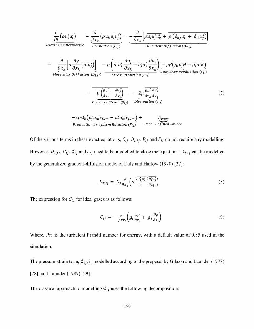
158

𝜕

𝜕𝑡(𝜌𝑢𝑖′𝑢𝑗′ )

⏟ 𝐿𝑜𝑐𝑎𝑙 𝑇𝑖𝑚𝑒 𝐷𝑒𝑟𝑖𝑣𝑎𝑡𝑖𝑣𝑒

+ 𝜕

𝜕𝑥𝑘(𝜌𝑢𝑘𝑢𝑖′𝑢𝑗′ )

⏟ 𝐶𝑜𝑛𝑣𝑒𝑐𝑡𝑖𝑜𝑛 (𝐶𝑖𝑗)

= −𝜕

𝜕𝑥𝑘[𝜌𝑢𝑖′𝑢𝑗′𝑢𝑘

′ + 𝑝 (𝛿𝑘𝑗𝑢𝑖′ + 𝛿𝑖𝑘𝑢𝑗′) ]

⏟ 𝑇𝑢𝑟𝑏𝑢𝑙𝑒𝑛𝑡 𝐷𝑖𝑓𝑓𝑢𝑠𝑖𝑜𝑛 (𝐷𝑇,𝑖𝑗)

+ 𝜕

𝜕𝑥𝑘[𝑢𝜕𝑦

𝜕𝑥𝑘(𝑢𝑖′𝑢𝑗′ )]

⏟ 𝑀𝑜𝑙𝑒𝑐𝑢𝑙𝑎𝑟 𝐷𝑖𝑓𝑓𝑢𝑠𝑖𝑜𝑛 (𝐷𝐿,𝑖𝑗)

− 𝜌 (𝑢𝑖′𝑢𝑘′ 𝜕𝑢𝑗

𝜕𝑥𝑘+ 𝑢𝑗′𝑢𝑘

′ 𝜕𝑢𝑗

𝜕𝑥𝑘)

⏟ 𝑆𝑡𝑟𝑒𝑠𝑠 𝑃𝑟𝑜𝑢𝑐𝑡𝑖𝑜𝑛 (𝑃𝑖𝑗)

− 𝜌𝛽(𝑔𝑖𝑢𝑗′𝜃 + 𝑔𝑖𝑢𝑖′𝜃)⏟ 𝐵𝑢𝑜𝑦𝑎𝑛𝑐𝑦 𝑃𝑟𝑜𝑑𝑢𝑐𝑡𝑖𝑜𝑛 (𝐺𝑖𝑗)

+ 𝑝 (𝜕𝑢𝑖

′

𝜕𝑥𝑗+𝜕𝑢𝑗

′

𝜕𝑥𝑖)

⏟ 𝑃𝑟𝑒𝑠𝑠𝑢𝑟𝑒 𝑆𝑡𝑟𝑎𝑖𝑛 (∅𝑖𝑗)

− 2𝜇

𝜕𝑢𝑖′

𝜕𝑥𝑘

𝜕𝑢𝑗′

𝜕𝑥𝑘

⏟ 𝐷𝑖𝑠𝑠𝑖𝑝𝑎𝑡𝑖𝑜𝑛 (𝜖𝑖𝑗)

(7)

−2𝜌𝛺𝑘(𝑢𝑗′𝑢𝑚′ 𝜖𝑖𝑘𝑚 + 𝑢𝑖′𝑢𝑚′ 𝜖𝑗𝑘𝑚)⏟ 𝑃𝑟𝑜𝑑𝑢𝑐𝑡𝑖𝑜𝑛 𝑏𝑦 𝑠𝑦𝑠𝑡𝑒𝑚 𝑅𝑜𝑡𝑎𝑡𝑖𝑜𝑛 (𝐹𝑖𝑗)

+ 𝑆𝑢𝑠𝑒𝑟⏟𝑈𝑠𝑒𝑟−𝐷𝑒𝑓𝑖𝑛𝑒𝑑 𝑆𝑜𝑢𝑟𝑐𝑒

Of the various terms in these exact equations, 𝐶𝑖𝑗, 𝐷𝐿,𝑖𝑗, 𝑃𝑖𝑗 and 𝐹𝑖𝑗 do not require any modelling.

However, 𝐷𝑇,𝑖𝑗, 𝐺𝑖𝑗, ∅𝑖𝑗 and 𝜖𝑖𝑗 need to be modelled to close the equations. 𝐷𝑇,𝑖𝑗 can be modelled

by the generalized gradient-diffusion model of Daly and Harlow (1970) [27]:

𝐷𝑇,𝑖𝑗 = 𝐶𝑠𝜕

𝜕𝑥𝑘(𝜌

𝑘𝑢𝑘′ 𝑢𝑖

′

𝜖


𝜕𝑥𝑙) (8)

The expression for 𝐺𝑖𝑗 for ideal gases is as follows:

𝐺𝑖𝑗 = −𝜇𝑡

𝜌𝑃𝑟𝑡(𝑔𝑖

𝜕𝜌

𝜕𝑥𝑗+ 𝑔𝑗

𝜕𝜌

𝜕𝑥𝑖) (9)

Where, 𝑃𝑟𝑡 is the turbulent Prandtl number for energy, with a default value of 0.85 used in the

simulation.

The pressure-strain term, ∅𝑖𝑗, is modelled according to the proposal by Gibson and Launder (1978)

[28], and Launder (1989) [29].

The classical approach to modelling ∅𝑖𝑗 uses the following decomposition:

159

∅𝑖𝑗 = ∅𝑖𝑗,1 + ∅𝑖𝑗,2 + ∅𝑖𝑗,𝑤 (10)

Where, ∅𝑖𝑗,1is the slow pressure-strain term, also known as the return-to-isotropy term, ∅𝑖𝑗,2 is the

rapid pressure-strain term, and ∅𝑖𝑗,𝑤 is the wall-reflection term.

The dissipation tensor, 𝜖𝑖𝑗, is modelled as:

𝜖𝑖𝑗 = 2

3𝛿𝑖𝑗(𝜌𝜖 + 𝑌𝑀) (11)

Where, 𝑌𝑀 = 2𝜌𝜖𝑀𝑡2 is an additional "dilatation dissipation'' term according to the model by

Sarkar and Lakshmanan (1991) [30].

Experimental Procedure

The existing flow loop at Memorial University is a 65-meter pipe open-cycle system. The liquid

can be pumped from the tank through the DN 80 (3-inch pipe). The experimental flow loop set-up

starts with an approximately 5-m-long clear horizontal test section, followed by 5-m-vertical clear

section and a consecutive variable inclination of a 3-m test section. These horizontal, vertical and

inclined pipe sections are installed in transparent PVC pipe for visualization. Instrumentation

includes several pressure and temperature sensors and flow meters for the gas and pipe line to

measure the individual gas and liquid flow rates. The air injection pipe is split into two different

sizes, DN 15 (0.5 inch) and DN 25 (1 inch), for different volumes of air flow. Electro-pneumatic

control valves are installed in the liquid and airline to facilitate control of the flow conditions and

to generate different flow regimes. The control of a flow loop is implemented through a fully

integrated online computer system, which also handles the data acquisition. Here in this work, data

for air-water two phase slug flow through a horizontal test section will be used. Figure 2 shows

the experimental setup.

160

(a)

(b)

Figure 2. Experimental set-up of the multiphase flow loop. (a) Simplified diagram; (b) Schematic

diagram

161

Table 1 lists the symbols used to outline the experimental set-up.

Table 1. Symbols used in flow loop (P&ID legend)

Simulation methodology

The computational grids for horizontal pipe are generated using ANSYS Fluent. Meshing is

finalized after conducting proper mesh independency check. Inflation is added near the wall to

observe more preciously the characteristics of different parameters near the wall. Shear stress

between wall surface and gas molecules is much higher and this inflation helps to create denser

meshing near wall. The length of the pipe is sufficient enough in this study to achieve a fully

developed flow at the outlet as minimum flow development section should be at least 50D (D =

internal diameter of pipe) [31]. One of the computational grid distributions of the pipe geometry

is shown in Figure 4.

ANSYS Inc. Fluent, ver. 16.2, ANSYS Inc. is used to build a CFD simulation model of pipeline

flow. A convergence value of 10-5 has been adopted for termination of iteration, this value is

selected by optimizing analysis to have the most satisfactory accuracy with less time. Figure 3

shows an analysis to discover the optimum convergence rate (between a range of 10-4 to 10-6) using

162

parameters (inlet velocity) from the experiment. SIMPLE algorithm is applied with the first and

second order upwind discretization method to have stability and confirm convergence in the

governing equations. Upwind discretization is a method that simulates numerically the direction

of the normal velocity in the flow field.

Figure 3. Optimum convergence rate analysis

Figure 4. Mesh distribution (cross section)

0

0.5

1

1.5

2

2.5

3

3.5

4

4.5

5

1.E-07 1.E-06 1.E-05 1.E-04

Pre

ssure

Gra

die

nt

(Pa/

m)

Convergent Rate

v=0.12 m/s

v=0.0707 m/s

v=0.0516 m/s

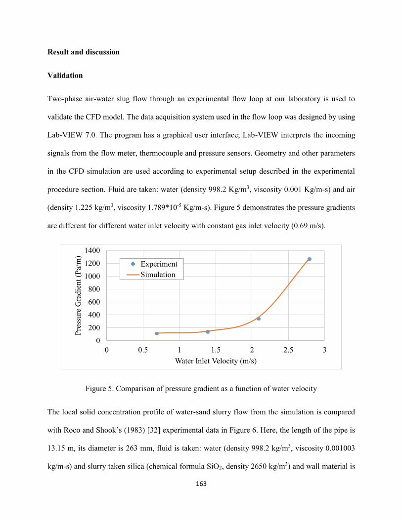
163

Result and discussion

Validation

Two-phase air-water slug flow through an experimental flow loop at our laboratory is used to

validate the CFD model. The data acquisition system used in the flow loop was designed by using

Lab-VIEW 7.0. The program has a graphical user interface; Lab-VIEW interprets the incoming

signals from the flow meter, thermocouple and pressure sensors. Geometry and other parameters

in the CFD simulation are used according to experimental setup described in the experimental

procedure section. Fluid are taken: water (density 998.2 Kg/m3, viscosity 0.001 Kg/m-s) and air

(density 1.225 kg/m3, viscosity 1.789*10-5 Kg/m-s). Figure 5 demonstrates the pressure gradients

are different for different water inlet velocity with constant gas inlet velocity (0.69 m/s).

Figure 5. Comparison of pressure gradient as a function of water velocity

The local solid concentration profile of water-sand slurry flow from the simulation is compared

with Roco and Shook’s (1983) [32] experimental data in Figure 6. Here, the length of the pipe is

13.15 m, its diameter is 263 mm, fluid is taken: water (density 998.2 kg/m3, viscosity 0.001003

kg/m-s) and slurry taken silica (chemical formula SiO2, density 2650 kg/m3) and wall material is

0

200

400

600

800

1000

1200

1400

0 0.5 1 1.5 2 2.5 3

Pre

ssure

Gra

die

nt

(Pa/

m)

Water Inlet Velocity (m/s)

Experiment

Simulation

164

aluminium (density 2800 kg/m3, roughness 0.2 mm). Grain size or mean particle diameter is 0.165

mm with mixture velocity 3.5 m/s and four different solid volumetric concentrations: 9.95%,

18.4%, 26.8% and 33.8% respectively.

Figure 6. Comparison of simulated and measured values of local volumetric concentration of

solid across vertical centreline

The simulated results are in good agreement with the experimental values. However, the simulated

values deviate from the experimental values. One probable reason for these deviations could be

the approximate value of the static settled concentration (packing limit) used during simulations,

as the value of 0.63 used is best suited to finer grain sizes only.

The pressure gradient of air-water-sand three-phase flow from the simulation is compared with

Fukuda and Shoji’s (1986) [12] experimental data. In the experiment length of the pipe is 2.9 m,

its diameter is 0.0416 m, fluids are taken: water (density 998.2 kg/m3, viscosity 0.001 kg/m-s),

silica sand particle (density 2650 kg/m3, mean particle diameter 74 µm) and air (density 1.225

-1.5

-1

-0.5

0

0.5

1

1.5

0 0.2 0.4 0.6

Ver

tica

l P

osi

tion (

Y/R

)



concentration)


concentration)


concentration)


concentration)

Experiment (9.95% vol

concentration)


concentration)


concentration)


concentration)

165

kg/m3, viscosity 1.789*10-5 kg/m-s). The pipe wall material is polycarbonate pipe (transparent,

smooth pipe). Figure 7 shows a comparison of the pressure gradient with the solid volume

concentration (Cv): 24.7% in slurry and 3 m/s slurry velocity at different gas velocities. In Figure

7, the average deviation of simulation data from experimental data is 2.1%, considering each point

with maximum 4.26% error at 1.36 m/s gas velocity in the pipeline. This shows very good

agreement (comparable error) with experiment.

Figure 7. Comparison of pressure gradient as a function of gas velocity

Parametric Analysis

After demonstrating very good and acceptable agreement of simulation with reference

experimental results, the approach is to analyse the flow behaviour at different condition of

independent parameters that affect multiphase flow through pipelines. In situ concentrations of

solid and diameter of pipeline are considered here as independent variables that can affect flow

behaviour.

2000

2500

3000

3500

4000

4500

5000

0 0.5 1 1.5 2

Pre

ssure

Gra

die

nt

(Pa/

m)

Gas Velocity (m/s)

Experiment (Cv = 24.7%)


166

Figure 8 shows the two-phase water-slurry flow contours of the local volumetric concentration

distribution of the solid phase in the vertical plane at the outlet cross-section for particle size of

slurry 0.165 mm and mixture velocity of 3.5 m/s at different efflux concentrations of solid slurry.

From contour analysis the region of highest solid concentration is located very near to the wall in

the lower half of the pipe cross section. This happened because of gravity in horizontal pipeline

which can lead to finding out the deposition velocity (i.e. minimum superficial velocity of mixture

to prevent accumulation of solids or waste in the pipeline).

(a) Solid volumetric concentration 9.95% (b) Solid volumetric concentration 18.4%

(c) Solid volumetric concentration 26.8% (d) Solid volumetric concentration 33.8%

Figure 8. Solid concentration distribution in the vertical plane at the outlet

167

Figure 9. Pressure gradient at different gas velocity and pipe diameter

Keeping sand in situ concentration in slurry, fluid viscosity and pipe wall roughness constant in

three phase air-water-slurry flow, Figure 9 graphically describes the change of pressure gradient

with the change in internal pipe diameter (D) and gas velocity.

The Darcy-Weisbach equation is as follows –

∆𝑃 = 𝑓𝐿

𝐷

𝜌𝑣2

2 (12)

where, ∆𝑃 is pressure drop, 𝑓 is friction factor, 𝐿 is pipe length, 𝐷 is internal diameter of the

pipeline, 𝜌 is fluid density and 𝑣 is fluid velocity.

According to Equation (12), the pressure gradient decreases with the increase in internal pipe

diameter, with the other parameters constant and the relation is inversely proportional. The

increasing rate of pressure gradient is lower for smaller pipe diameters, but the trend of the

increasing rate is almost the same. The pipeline should not be manufactured with a diameter size

lower than a specific limit, which produces a maximum level of pressure drop required by industry.

0

1000

2000

3000

4000

5000

6000

0 0.5 1 1.5 2 2.5 3

Pre

ssure

Gra

die

nt

(Pa/

m)

Gas Velocity (m/s)

Simulation (D = 41.5 mm)

Simulation (D = 30 mm)

Simulation (D = 50 mm)

168

Conclusion

This CFD simulation approach to multiphase flow through a horizontal pipeline demonstrates

some good agreements and outcomes, with reference to experimental works. With the aim of

building a model that can be applied in practical problems with fewer parameter boundary

limitations, some analysis is performed under different conditions, after validating the developed

model. A few of the approaches are listed below:

• Building a CFD model with Eulerian multiphase and RSM turbulence closure to simulate

multiphase flow through a horizontal pipeline.

• Discussing the numerical explanation of CFD modelling and its assumptions with valid

references.

• Demonstrating, with a diagram, an experimental flow loop which is sited in our laboratory.

• Simulating two-phase water-air slug flow and comparing with our own experiment.

• Validating two-phase water-sand slurry flow with reference to the experimental data.

• Validating three-phase air-water-sand flow with reference the experimental data; this also

demonstrates the effect of adding air into two-phase slurry flow.

• Conducting a few parametric studies with two-phase and three-phase flow. Contour

distribution of the in-situ concentration of sand and pressure gradient are used as output

parameters to analyze the effects of changing parameters. The output shows similarity with

developed theories and empirical correlations.

The study is ongoing with parametric analysis. CFD errors need to be reduced by focusing more

on the choice of different coefficients and constants such as the coefficient of lift, coefficient of

169

drag, restitution coefficient and wall boundary conditions. The effect of vibration due to fluid flow

will be a future task for this project.

Acknowledgements

The authors wish to acknowledge the Faculty of Engineering and Applied Science of Memorial

University and ANSYS Inc. for help during this project.

References

[1]. Geilikman, M. B., & Dusseault, M. B. (1997). Fluid rate enhancement from massive sand

production in heavy-oil reservoirs. Journal of Petroleum Science and Engineering, 17(1), 5-

18.

[2]. Rajnauth, J., & Barrufet, M. (2012). Monetizing gas: Focusing on developments in gas

hydrate as a mode of transportation. Energy Science and Technology, 4(2), 61-68.

[3]. Miao, Z., Shastri, Y., Grift, T., Hansen, A., & Ting, K. (2012). Lignocellulosic biomass

feedstock transportation alternatives, logistics, equipment configurations, and

modeling. Biofuels, Bioproducts and Biorefining, 6(3), 351-362.

[4]. Bello, O., Reinicke, K., & Teodoriu, C. (2005). Particle holdup profiles in horizontal gas‐

liquid‐solid multiphase flow pipeline. Chemical Engineering & Technology, 28(12), 1546-

1553.

[5]. Mao, F., Desir, F. K., & Ebadian, M. A. (1997). Pressure drop measurement and correlation

for three-phase flow of simulated nuclear waste in a horizontal pipe. International journal of

multiphase flow, 23(2), 397-402.

170

[6]. Al-Lababidi, S., Addali, A., Yeung, H., Mba, D., & Khan, F. (2009). Gas void fraction

measurement in two-phase gas/liquid slug flow using acoustic emission technology. Journal

of Vibration and Acoustics, 131(6), 064501.

[7]. Czapp, M., Utschick, M., Rutzmoser, J., & Sattelmayer, T. (2012, July). Investigations on

slug flow in a horizontal pipe using stereoscopic particle image velocimetry and CFD

simulation with volume of fluid method. In 2012 20th International Conference on Nuclear

Engineering and the ASME 2012 Power Conference (pp. 477-486). American Society of


[8]. Pouranfard, A. R., Mowla, D., & Esmaeilzadeh, F. (2015). An experimental study of drag

reduction by nanofluids in slug two-phase flow of air and water through horizontal

pipes. Chinese Journal of Chemical Engineering, 23(3), 471-475.

[9]. Sanders, R., Schaan, J., & McKibben, M. (2007). Oil sand slurry conditioning tests in a

100 mm pipeline loop. Canadian Journal of Chemical Engineering, 85(5), 756-764.

[10]. Scott, D. S., & Rao, P. K. (1971). Transport of solids by gas‐liquid mixtures in horizontal

pipes. The Canadian Journal of Chemical Engineering, 49(3), 302-309.

[11]. Toda, M., Shimazaki, K., & Maeda, S. (1978). Pressure drop of three-phase flow in horizontal

pipes. Kagaku Kogaku Ronbunshu, 4, 56-62.

[12]. Fukuda, T., & Shoji, Y. (1986). Pressure drop and heat transfer for tree phase flow: 1st report,

flow in horizontal pipes. Bulletin of JSME, 29(256), 3421-3426.

[13]. Kago, T., Saruwatari, T., Kashima, M., Morooka, S., & Kato, Y. (1986). Heat transfer in

horizontal plug and slug flow for gas-liquid and gas-slurry systems. Journal of Chemical

Engineering of Japan, 19(2), 125-131.

171

[14]. Toda, M., & Konno, H. (1987). Fundamentals of gas-liquid-solid three phase flow. Japanese

Journal of Multiphase Flow, 1(2), 139-156.

[15]. Gillies, R. G., McKibben, M. J., & Shook, C. A. (1997). Pipeline flow of gas, liquid and sand

mixtures at low velocities. Journal of Canadian Petroleum Technology, 36(09).

[16]. Bello, O. O., Udong, I. N., Falcone, G., & Teodoriu, C. (2010, January). Hydraulic analysis

of gas/oil/sand flow in horizontal wells. In SPE Latin American and Caribbean Petroleum

Engineering Conference. Society of Petroleum Engineers.

[17]. Rahman, M. A., Adane, K. F., & Sanders, R. S. (2013). An improved method for applying

the Lockhart–Martinelli correlation to three‐phase gas–liquid–solid horizontal pipeline

flows. The Canadian Journal of Chemical Engineering, 91(8), 1372-1382.

[18]. Annaland, M., Deen, N. G., & Kuipers, J. A. M. (2005). Numerical simulation of gas–liquid–

solid flows using a combined front tracking and discrete particle method. Chemical

Engineering Science, 60(22), 6188-6198.

[19]. Washino, Tan, Salman, & Hounslow. (2011). Direct numerical simulation of solid–liquid–

gas three-phase flow: Fluid–solid interaction. Powder Technology, 206(1), 161-169.

[20]. Liu, X., Aramaki, Y., Guo, L., & Morita, K. (2015). Numerical simulation of gas–liquid–

solid three-phase flow using particle methods. Journal of Nuclear Science and

Technology, 52(12), 1480-1489.

[21]. Orell, A. (2007). The effect of gas injection on the hydraulic transport of slurries in horizontal

pipes. Chemical Engineering Science, 62(23), 6659-6676.

[22]. Alder, B. J., & Wainwright, T. E. (1960). Studies in molecular dynamics. II. Behavior of a

small number of elastic spheres. The Journal of Chemical Physics, 33(5), 1439-1451.

172

[23]. Syamlal, M., Rogers, W., & O’Brien, T. J. (1993). MFIX documentation: Theory

guide. National Energy Technology Laboratory, Department of Energy, Technical Note

DOE/METC-95/1013 and NTIS/DE95000031.

[24]. Vijiapurapu, S., & Cui, J. (2010). Performance of turbulence models for flows through rough

pipes. Applied Mathematical Modelling, 34(6), 1458-1466.

[25]. Markatos, N. C. (1986). The mathematical modelling of turbulent flows. Applied

Mathematical Modelling, 10(3), 190-220.

[26]. Kaushal, D. R., Sato, K., Toyota, T., Funatsu, K., & Tomita, Y. (2005). Effect of particle size

distribution on pressure drop and concentration profile in pipeline flow of highly

concentrated slurry. International Journal of Multiphase Flow, 31(7), 809-823.

[27]. Daly, B. J., & Harlow, F. H. (1970). Transport equations in turbulence. Physics of Fluids

(1958-1988), 13(11), 2634-2649.

[28]. Gibson, M. M., & Launder, B. E. (1978). Ground effects on pressure fluctuations in the

atmospheric boundary layer. Journal of Fluid Mechanics,86(03), 491-511.

[29]. Launder, B. E. (1989). Second-moment closure: present… and future?- International Journal

of Heat and Fluid Flow, 10(4), 282-300.

[30]. Sarkar, S., & Lakshmanan, B. (1991). Application of a Reynolds stress turbulence model to

the compressible shear layer. AIAA Journal, 29(5), 743-749.

[31]. Brown, N. P., & Heywood, N. I. (Eds.). (1991). Slurry Handling: Design of solid-liquid

systems. Springer Science & Business Media.

[32]. Roco, M. C., & Shook, C. A. (1983). Modeling of slurry flow: the effect of particle size. The


173

Appendix 4. Data Tables

Table 1. Parametric Study Chart with Single Phase Fluid (Chapter 2)

Controlled Variables CFD Results

Reynolds

number

(Re=dHVρ/μ)

Rotational speed

(rpm)

Eccentricity (%) Pressure gradient

(Pa/m)

20000 0 0 82

40000 0 0 150

50000 0 0 230

60000 0 0 320

80000 0 0 557.575

100000 0 0 920.161

20000 50 0 103

40000 50 0 158

50000 50 0 234

60000 50 0 324

80000 50 0 562.112

100000 50 0 923.5

20000 100 0 165

40000 100 0 209

50000 100 0 269

60000 100 0 345

174

80000 100 0 595.795

100000 100 0 933.455

20000 150 0 275

40000 150 0 293

50000 150 0 343

60000 150 0 407

80000 150 0 645.529

100000 150 0 966.1

20000 0 25 77

40000 0 25 140

50000 0 25 214

60000 0 25 299

80000 0 25 555.578

100000 0 25 902.474

20000 50 25 97

40000 50 25 150

50000 50 25 221

60000 50 25 304

80000 50 25 559.412

100000 50 25 906.422

20000 100 25 169

40000 100 25 206

50000 100 25 259

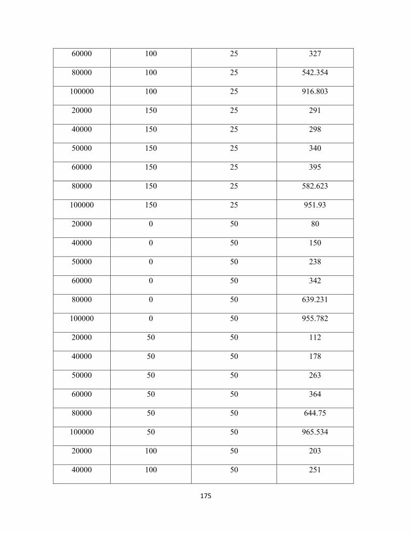
175

60000 100 25 327

80000 100 25 542.354

100000 100 25 916.803

20000 150 25 291

40000 150 25 298

50000 150 25 340

60000 150 25 395

80000 150 25 582.623

100000 150 25 951.93

20000 0 50 80

40000 0 50 150

50000 0 50 238

60000 0 50 342

80000 0 50 639.231

100000 0 50 955.782

20000 50 50 112

40000 50 50 178

50000 50 50 263

60000 50 50 364

80000 50 50 644.75

100000 50 50 965.534

20000 100 50 203

40000 100 50 251

176

50000 100 50 323

60000 100 50 416

80000 100 50 689.054

100000 100 50 1003.29

20000 150 50 355

40000 150 50 373

50000 150 50 428

60000 150 50 505

80000 150 50 750.208

100000 150 50 1056.07

20000 0 75 71

40000 0 75 135

50000 0 75 215

60000 0 75 310

80000 0 75 574.076

100000 0 75 907.722

20000 50 75 123

40000 50 75 197

50000 50 75 288

60000 50 75 395

80000 50 75 680.247

100000 50 75 1013.64

20000 100 75 231

177

40000 100 75 296

50000 100 75 388

60000 100 75 501

80000 100 75 810.132

100000 100 75 1166.54

20000 150 75 401

40000 150 75 449

50000 150 75 528

60000 150 75 631

80000 150 75 948.062

100000 150 75 1313.03

178

Table 2. Parametric Study Chart with Two Phase Fluid (Chapter 2)

Controlled Variables CFD Results

Reynolds

number

(Re=dHVρ/μ)

Rotational

speed

(rpm)

Eccentricity

(%)

Particle Input

Concentration

(%)

Particle

Size

(mm)

Pressure

gradient

(Pa/m)

Maximum Bed

Concentration

near bottom

wall (%)

40000 stationary Concentric 5 0.05 766.966 58.12








40000 stationary Concentric 5 0.1 767.674 58








179









40000 150 Concentric 5 0.05 812.232 57.79

70000 150 Concentric 5 0.05 888.334 21.84

100000 150 Concentric 5 0.05 1162.98 12.33

200000 150 Concentric 5 0.05 3151.97 7.48

40000 150 Concentric 20 0.05 812.265 57.74

70000 150 Concentric 20 0.05 888.189 21.65

100000 150 Concentric 20 0.05 1162.52 12.32

200000 150 Concentric 20 0.05 3151.46 7.47

40000 150 Concentric 5 0.1 808.946 53.66

70000 150 Concentric 5 0.1 886.414 41.42

100000 150 Concentric 5 0.1 1155.53 25.81

200000 150 Concentric 5 0.1 3160.58 10.17

40000 150 Concentric 20 0.1 810.85 51.43

70000 150 Concentric 20 0.1 886.051 41.47

100000 150 Concentric 20 0.1 1156.06 25.85

180

200000 150 Concentric 20 0.1 3149.8 10.16

40000 150 Concentric 5 0.005 799.978 5.27

70000 150 Concentric 5 0.005 882.585 5.14

100000 150 Concentric 5 0.005 1162.34 5.1

200000 150 Concentric 5 0.005 3166.04 5.06

40000 150 Concentric 20 0.005 799.909 5.27

70000 150 Concentric 20 0.005 882.953 5.14

100000 150 Concentric 20 0.005 1162.38 5.1

200000 150 Concentric 20 0.005 3146.69 5.06

85000 stationary 50 5 0.05 1042.12 33.71

100000 stationary 50 5 0.05 1198.23 26.03

200000 stationary 50 5 0.05 3255.59 9.96

300000 stationary 50 5 0.05 6848.14 7.76

85000 stationary 50 20 0.05 1055.6 33.46

100000 stationary 50 20 0.05 1206.28 24.9

200000 stationary 50 20 0.05 3278.31 9.9

300000 stationary 50 20 0.05 6693.65 7.78

85000 stationary 50 5 0.1 1011.03 26.39

100000 stationary 50 5 0.1 1263.45 23.56

200000 stationary 50 5 0.1 3170.89 9.91

300000 stationary 50 5 0.1 6479.87 6.83

85000 stationary 50 20 0.1 1016.64 30.3

100000 stationary 50 20 0.1 1179.16 23.6

181

200000 stationary 50 20 0.1 3180.33 10.62

300000 stationary 50 20 0.1 6636.22 7.2

85000 stationary 50 5 0.005 1036.05 5.35

100000 stationary 50 5 0.005 1192.55 5.3

200000 stationary 50 5 0.005 3184.09 5.15

300000 stationary 50 5 0.005 6544.09 5.1

85000 stationary 50 20 0.005 1035.73 5.36

100000 stationary 50 20 0.005 1195.77 5.3

200000 stationary 50 20 0.005 3186.63 5.15

300000 stationary 50 20 0.005 6519.47 5.1

85000 150 50 5 0.05 1095.77 32.5

100000 150 50 5 0.05 1259.55 24.06

200000 150 50 5 0.05 3342.23 10.21

300000 150 50 5 0.05 6794.4 7.72

85000 150 50 20 0.05 1096.93 29.37

100000 150 50 20 0.05 1277.49 22.62

200000 150 50 20 0.05 3352.92 9.85

300000 150 50 20 0.05 6849.01 7.55

85000 150 50 5 0.1 1075.24 25.28

100000 150 50 5 0.1 1226.04 24.57

200000 150 50 5 0.1 3196.13 9.8

300000 150 50 5 0.1 6533.21 6.94

85000 150 50 20 0.1 1071.57 25.25

182

100000 150 50 20 0.1 1244.69 22.86

200000 150 50 20 0.1 3216.8 10.19

300000 150 50 20 0.1 6656.04 7.32

85000 150 50 5 0.005 1092.88 5.35

100000 150 50 5 0.005 1257.26 5.29

200000 150 50 5 0.005 3246.63 5.15

300000 150 50 5 0.005 6567.77 5.1

85000 150 50 20 0.005 1091.97 5.35

100000 150 50 20 0.005 1261.21 5.29

200000 150 50 20 0.005 3243.02 5.15

300000 150 50 20 0.005 6561.63 5.1

A Comprehensive Study on Multiphase Flow through Pipeline ...

Documents

Transcript of A Comprehensive Study on Multiphase Flow through Pipeline ...