Multicomponent Multiphase LB Models

Multi- Component Multiphase

Miscible Fluids/Diffusion (No Interaction)

Immiscible Fluids

Single Component Multiphase

Single Phase

(No Interaction)

Num

ber

of

Com

pone

ntsInteraction Strength

Nat

ure

of

Inte

ract

ion

Attractive

Repulsive

LowHigh

Inherent Parallelism

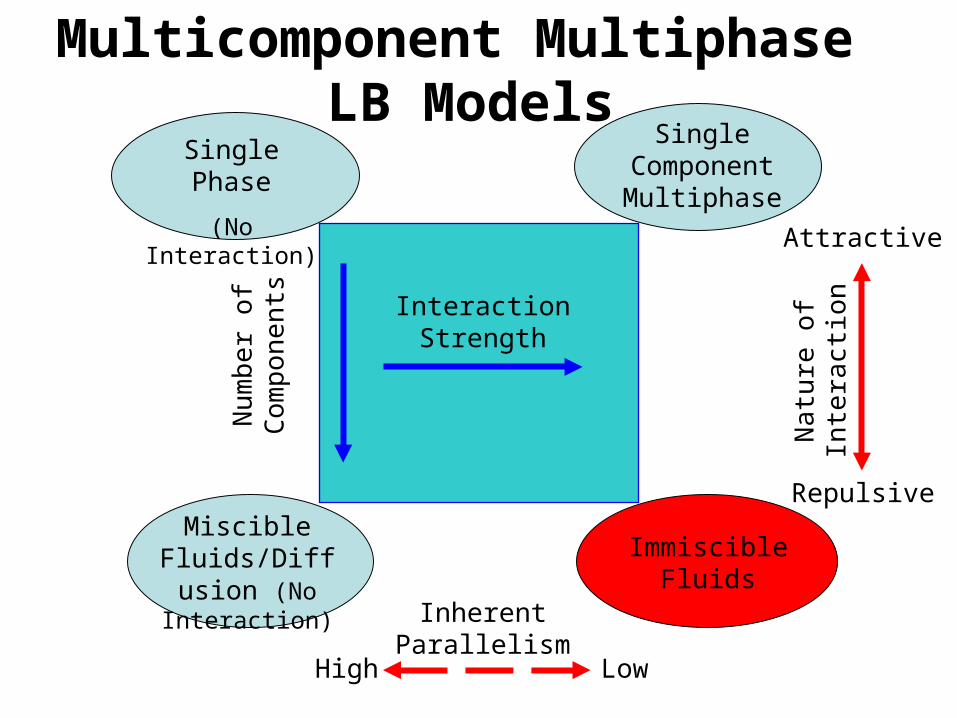
Adding a component/substance

Often just need another loop:

• for( subs=0; subs<NUM_FLUID_COMPONENTS; subs++)• for( j=0; j<LY; j++)• for( i=0; i<LX; i++)• {

…

• }

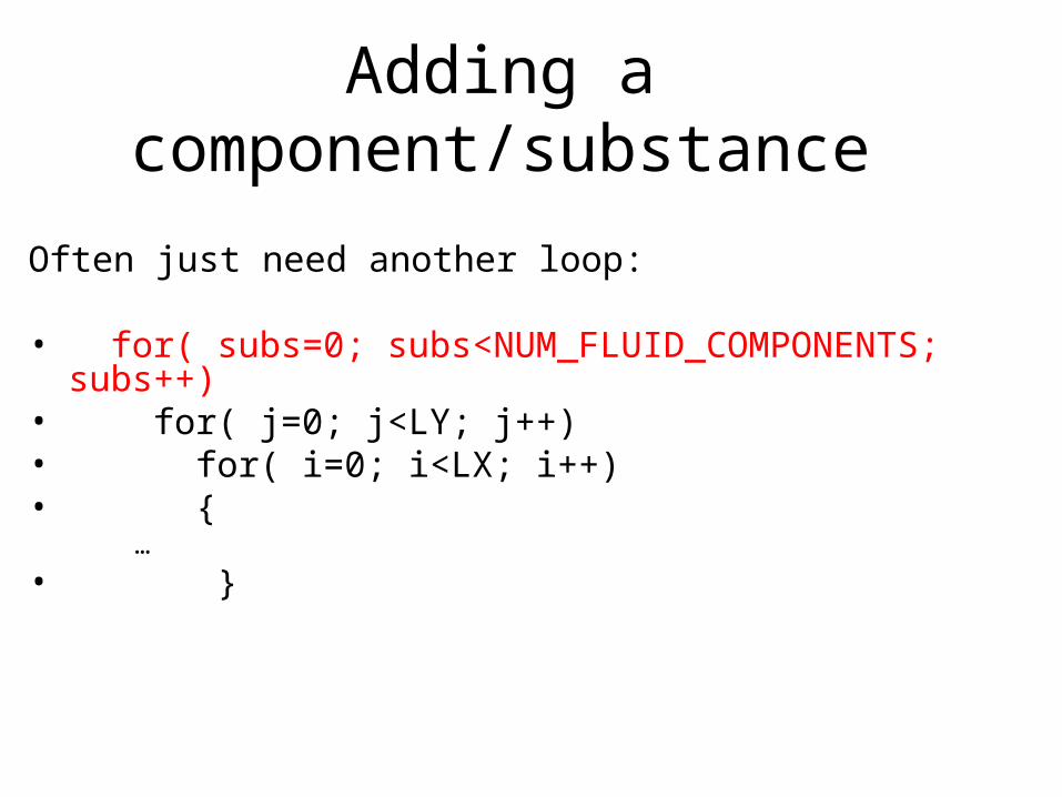
One composite u for feq calculation

(Eqn. 95 in Sukop and Thorne; note error in 2006 printing)

• // Compute density, Eq. (97), and the sums used (below) • // in the velocities.• for( subs=0; subs<NUM_FLUID_COMPONENTS; subs++)• for( j=0; j<LY; j++)• for( i=0; i<LX; i++)• {• rhoij[subs] = 0.;• u_xij[subs] = 0.;• u_yij[subs] = 0.;• • if( !is_solid_node[j][i]) {• for( a=0; a<9; a++) {• rhoij[subs] += ftemp_ij[a];• u_xij[subs] += ex[a]*ftemp_ij[a];• u_yij[subs] += ey[a]*ftemp_ij[a]; } }• }

1

1

' aaaf e

u

8

0

1

aaaf eu

8

0aaf

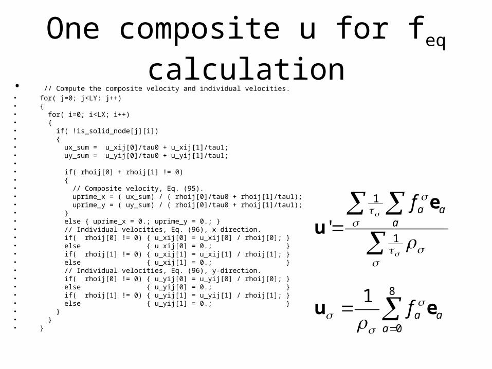
One composite u for feq calculation• // Compute the composite velocity and individual velocities.• for( j=0; j<LY; j++)• {• for( i=0; i<LX; i++)• {• if( !is_solid_node[j][i])• {• ux_sum = u_xij[0]/tau0 + u_xij[1]/tau1;• uy_sum = u_yij[0]/tau0 + u_yij[1]/tau1;• • if( rhoij[0] + rhoij[1] != 0)• {• // Composite velocity, Eq. (95).• uprime_x = ( ux_sum) / ( rhoij[0]/tau0 + rhoij[1]/tau1);• uprime_y = ( uy_sum) / ( rhoij[0]/tau0 + rhoij[1]/tau1);• }• else { uprime_x = 0.; uprime_y = 0.; }• // Individual velocities, Eq. (96), x-direction.• if( rhoij[0] != 0) { u_xij[0] = u_xij[0] / rhoij[0]; }• else { u_xij[0] = 0.; }• if( rhoij[1] != 0) { u_xij[1] = u_xij[1] / rhoij[1]; }• else { u_xij[1] = 0.; }• // Individual velocities, Eq. (96), y-direction.• if( rhoij[0] != 0) { u_yij[0] = u_yij[0] / rhoij[0]; }• else { u_yij[0] = 0.; }• if( rhoij[1] != 0) { u_yij[1] = u_yij[1] / rhoij[1]; }• else { u_yij[1] = 0.; }• }• }• }

1

1

' aaaf e

u

8

0

1

aaaf eu

Interparticle Forces

• // Compute fluid-fluid interaction force, equation (98), • // (assuming periodic domain).• //• // We begin by computing psi even though in this implementation• // it is the same as rho. A different function of rho could• // be substituted here.• for( subs=0; subs<NUM_FLUID_COMPONENTS; subs++)• for( j=0; j<LY; j++)• for( i=0; i<LX; i++)• if( !is_solid_node[j][i])• {• psi[subs][j][i] = rho[subs][j][i];• }•

a

aaa ttwtG eexxxF ),(),()(

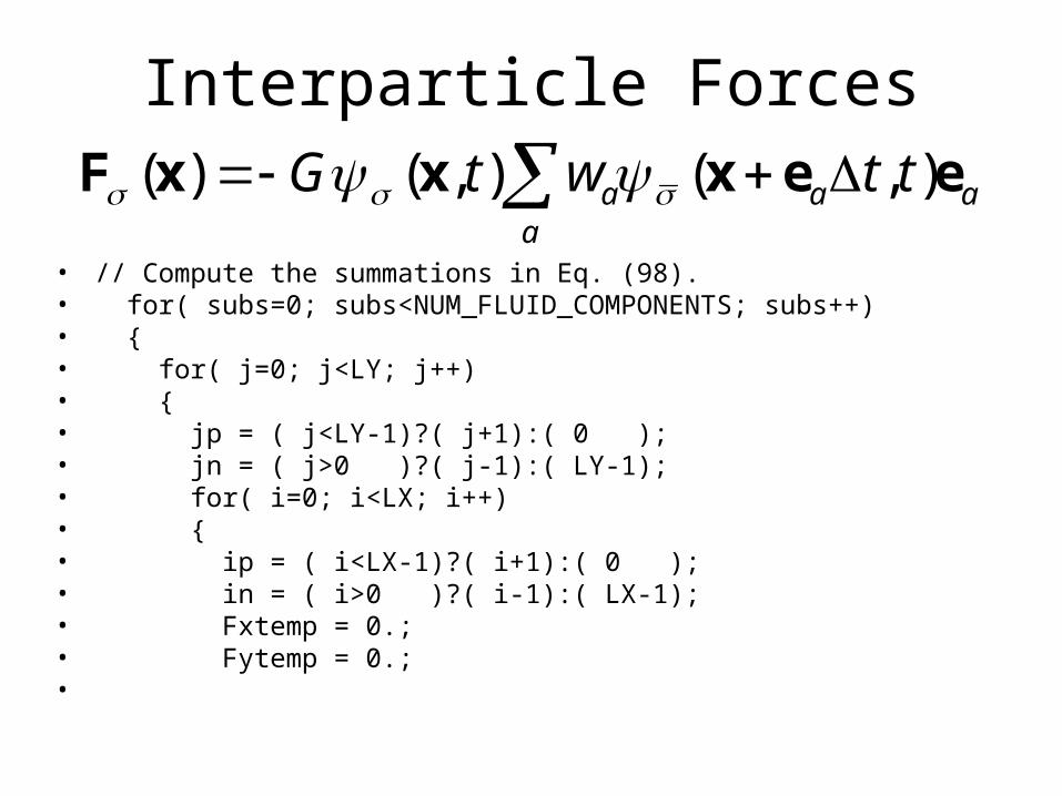
Interparticle Forces

• // Compute the summations in Eq. (98).• for( subs=0; subs<NUM_FLUID_COMPONENTS; subs++)• {• for( j=0; j<LY; j++)• {• jp = ( j<LY-1)?( j+1):( 0 );• jn = ( j>0 )?( j-1):( LY-1);• for( i=0; i<LX; i++)• {• ip = ( i<LX-1)?( i+1):( 0 );• in = ( i>0 )?( i-1):( LX-1);• Fxtemp = 0.;• Fytemp = 0.;•

a

aaa ttwtG eexxxF ),(),()(

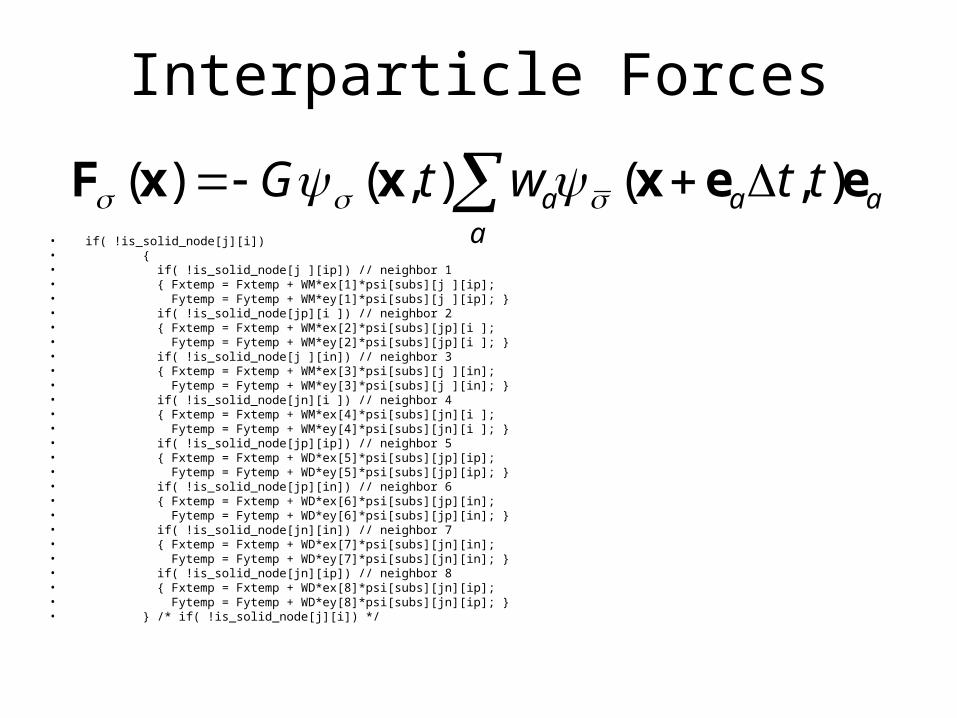
Interparticle Forces

• if( !is_solid_node[j][i])• {• if( !is_solid_node[j ][ip]) // neighbor 1• { Fxtemp = Fxtemp + WM*ex[1]*psi[subs][j ][ip];• Fytemp = Fytemp + WM*ey[1]*psi[subs][j ][ip]; }• if( !is_solid_node[jp][i ]) // neighbor 2• { Fxtemp = Fxtemp + WM*ex[2]*psi[subs][jp][i ];• Fytemp = Fytemp + WM*ey[2]*psi[subs][jp][i ]; }• if( !is_solid_node[j ][in]) // neighbor 3• { Fxtemp = Fxtemp + WM*ex[3]*psi[subs][j ][in];• Fytemp = Fytemp + WM*ey[3]*psi[subs][j ][in]; }• if( !is_solid_node[jn][i ]) // neighbor 4• { Fxtemp = Fxtemp + WM*ex[4]*psi[subs][jn][i ];• Fytemp = Fytemp + WM*ey[4]*psi[subs][jn][i ]; }• if( !is_solid_node[jp][ip]) // neighbor 5• { Fxtemp = Fxtemp + WD*ex[5]*psi[subs][jp][ip];• Fytemp = Fytemp + WD*ey[5]*psi[subs][jp][ip]; }• if( !is_solid_node[jp][in]) // neighbor 6• { Fxtemp = Fxtemp + WD*ex[6]*psi[subs][jp][in];• Fytemp = Fytemp + WD*ey[6]*psi[subs][jp][in]; }• if( !is_solid_node[jn][in]) // neighbor 7• { Fxtemp = Fxtemp + WD*ex[7]*psi[subs][jn][in];• Fytemp = Fytemp + WD*ey[7]*psi[subs][jn][in]; }• if( !is_solid_node[jn][ip]) // neighbor 8• { Fxtemp = Fxtemp + WD*ex[8]*psi[subs][jn][ip];• Fytemp = Fytemp + WD*ey[8]*psi[subs][jn][ip]; }• } /* if( !is_solid_node[j][i]) */

a

aaa ttwtG eexxxF ),(),()(

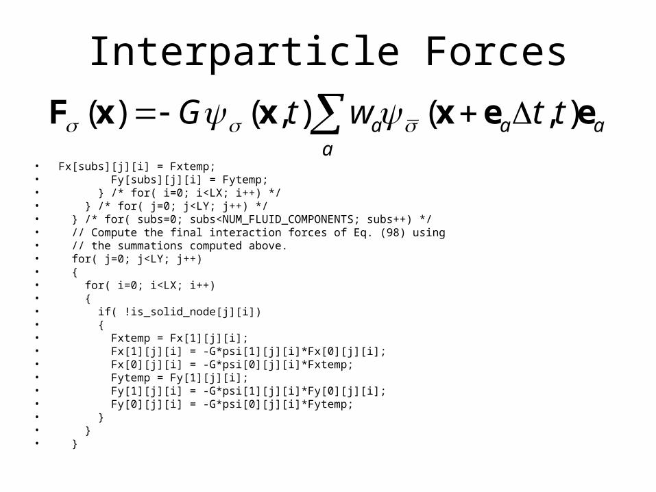
Interparticle Forces

• Fx[subs][j][i] = Fxtemp;• Fy[subs][j][i] = Fytemp;• } /* for( i=0; i<LX; i++) */• } /* for( j=0; j<LY; j++) */• } /* for( subs=0; subs<NUM_FLUID_COMPONENTS; subs++) */• // Compute the final interaction forces of Eq. (98) using• // the summations computed above.• for( j=0; j<LY; j++)• {• for( i=0; i<LX; i++)• {• if( !is_solid_node[j][i])• {• Fxtemp = Fx[1][j][i];• Fx[1][j][i] = -G*psi[1][j][i]*Fx[0][j][i];• Fx[0][j][i] = -G*psi[0][j][i]*Fxtemp;• Fytemp = Fy[1][j][i];• Fy[1][j][i] = -G*psi[1][j][i]*Fy[0][j][i];• Fy[0][j][i] = -G*psi[0][j][i]*Fytemp;• }• }• }

a

aaa ttwtG eexxxF ),(),()(

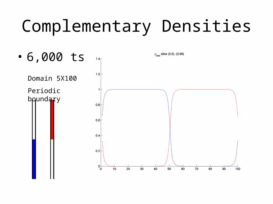
Complementary Densities

• 6,000 ts

Domain 5X100

Periodic boundary

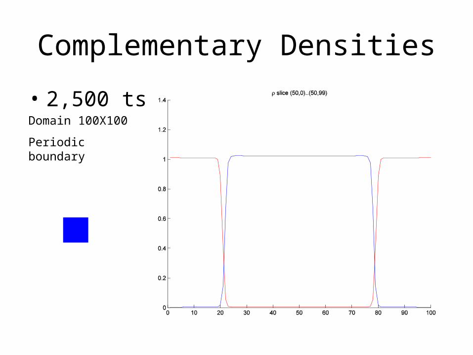
Complementary Densities

• 2,500 tsDomain 100X100

Periodic boundary

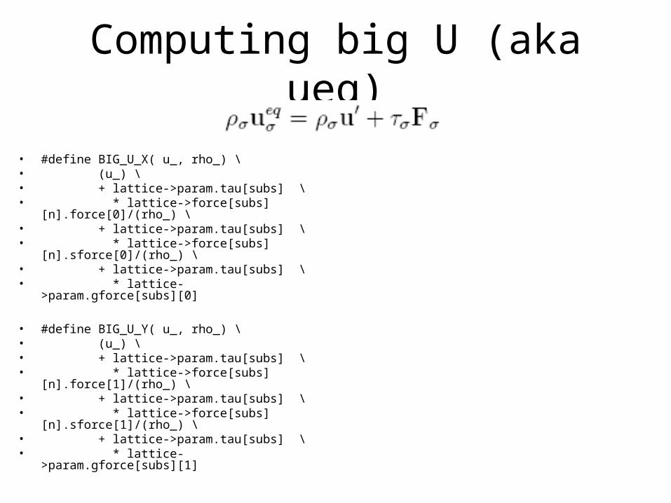
Computing big U (aka ueq)

• #define BIG_U_X( u_, rho_) \• (u_) \• + lattice->param.tau[subs] \• *

lattice->force[subs][n].force[0]/(rho_) \• + lattice->param.tau[subs] \• *

lattice->force[subs][n].sforce[0]/(rho_) \• + lattice->param.tau[subs] \• * lattice->param.gforce[subs][0]

• #define BIG_U_Y( u_, rho_) \• (u_) \• + lattice->param.tau[subs] \• *

lattice->force[subs][n].force[1]/(rho_) \• + lattice->param.tau[subs] \• *

lattice->force[subs][n].sforce[1]/(rho_) \• + lattice->param.tau[subs] \• * lattice->param.gforce[subs][1]

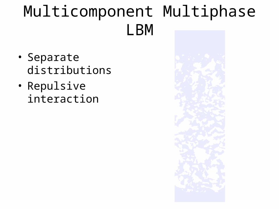
Multicomponent Multiphase LBM

• Separate distributions• Repulsive interaction

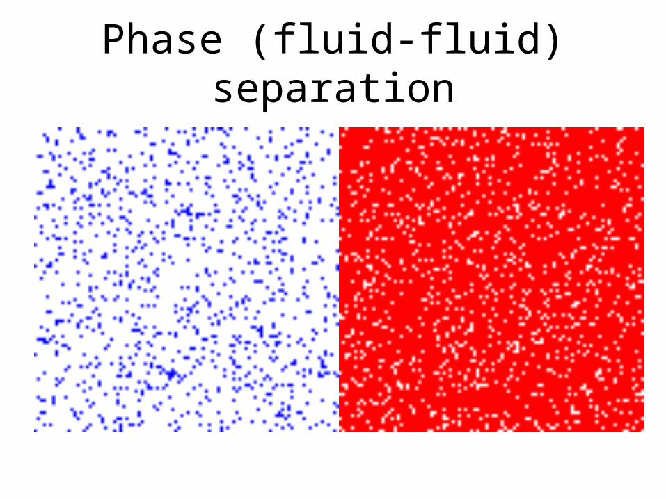
Phase (fluid-fluid) separation

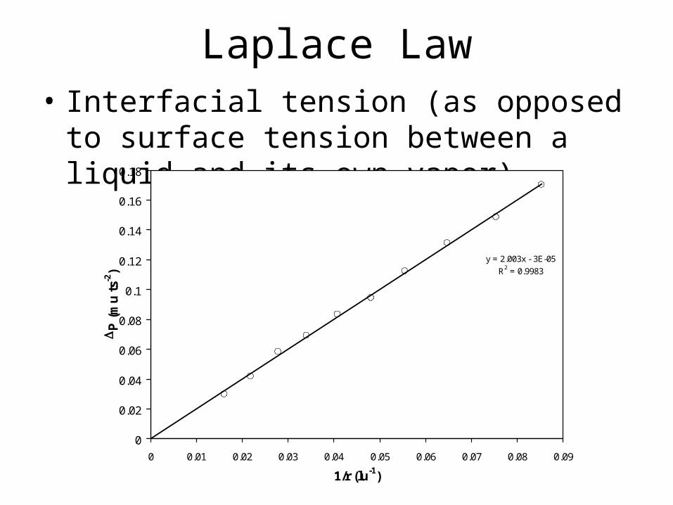
Laplace Law• Interfacial tension (as opposed to surface

tension between a liquid and its own vapor)

y = 2.003x - 3E-05

R2 = 0.9983

0

0.02

0.04

0.06

0.08

0.1

0.12

0.14

0.16

0.18

0 0.01 0.02 0.03 0.04 0.05 0.06 0.07 0.08 0.09

1/r (lu-1)

P

(m

u t

s-2)

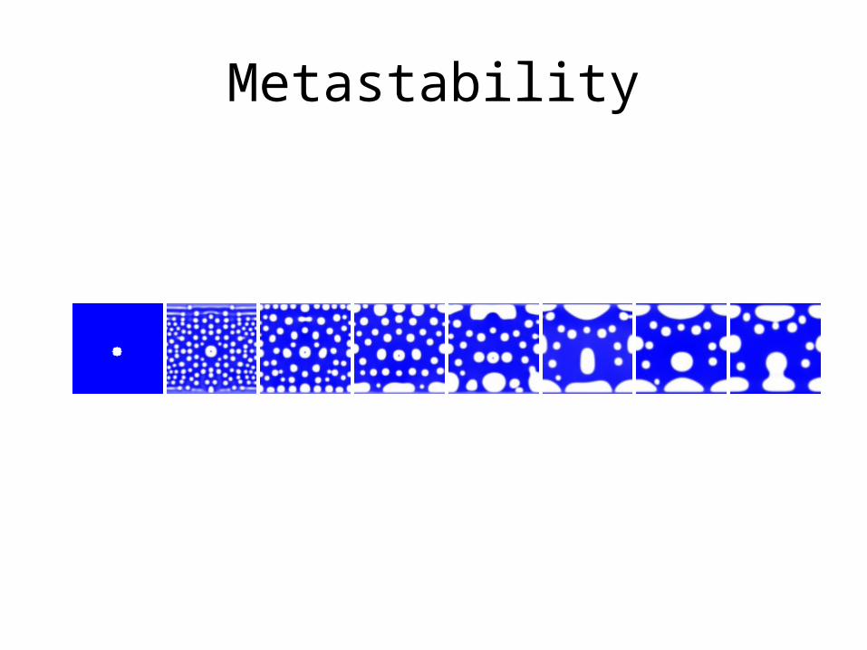
Metastability

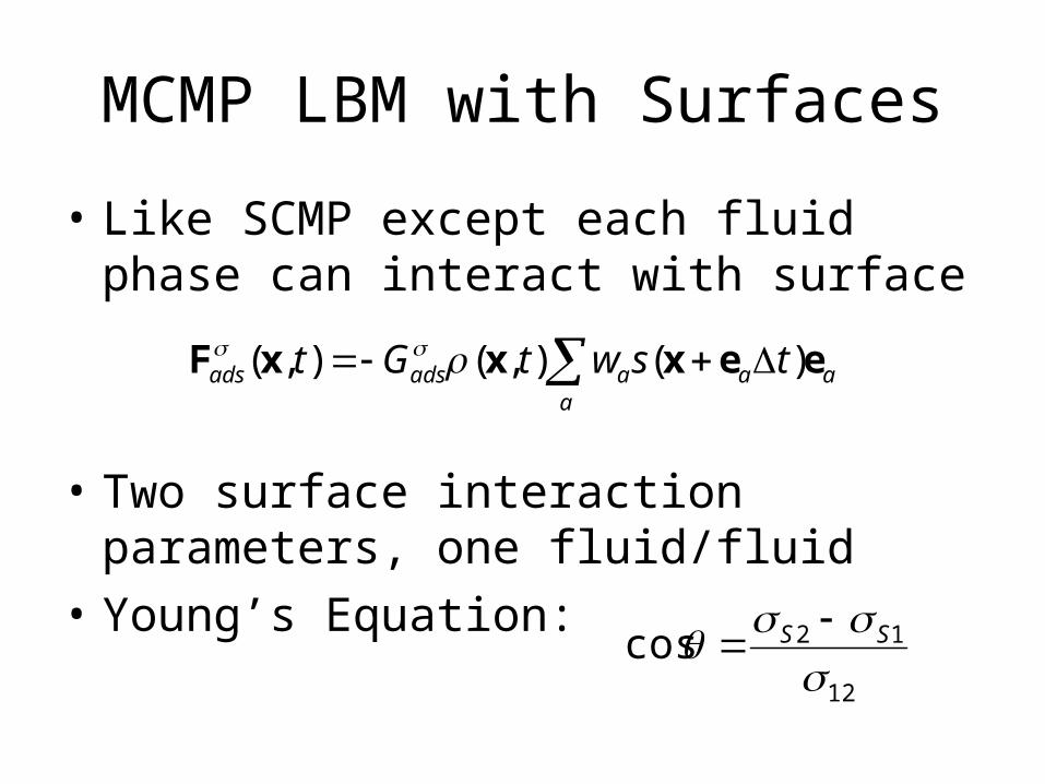
MCMP LBM with Surfaces

• Like SCMP except each fluid phase can interact with surface

• Two surface interaction parameters, one fluid/fluid

• Young’s Equation:

12

12cos

SS

a

aaaadsads tswtGt eexxxF )(),(),(

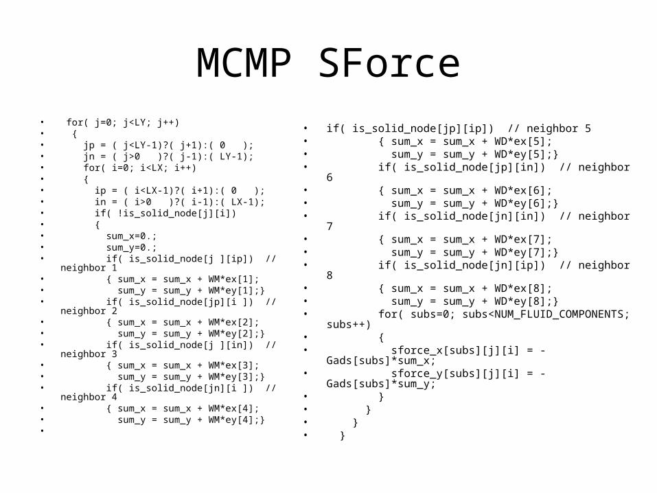
MCMP SForce• for( j=0; j<LY; j++)• {• jp = ( j<LY-1)?( j+1):( 0 );• jn = ( j>0 )?( j-1):( LY-1);• for( i=0; i<LX; i++)• {• ip = ( i<LX-1)?( i+1):( 0 );• in = ( i>0 )?( i-1):( LX-1);• if( !is_solid_node[j][i]) • {• sum_x=0.;• sum_y=0.;• if( is_solid_node[j ][ip]) // neighbor 1• { sum_x = sum_x + WM*ex[1];• sum_y = sum_y + WM*ey[1];}• if( is_solid_node[jp][i ]) // neighbor 2• { sum_x = sum_x + WM*ex[2];• sum_y = sum_y + WM*ey[2];}• if( is_solid_node[j ][in]) // neighbor 3• { sum_x = sum_x + WM*ex[3];• sum_y = sum_y + WM*ey[3];}• if( is_solid_node[jn][i ]) // neighbor 4• { sum_x = sum_x + WM*ex[4];• sum_y = sum_y + WM*ey[4];}•

• if( is_solid_node[jp][ip]) // neighbor 5• { sum_x = sum_x + WD*ex[5];• sum_y = sum_y + WD*ey[5];}• if( is_solid_node[jp][in]) // neighbor 6• { sum_x = sum_x + WD*ex[6];• sum_y = sum_y + WD*ey[6];}• if( is_solid_node[jn][in]) // neighbor 7• { sum_x = sum_x + WD*ex[7];• sum_y = sum_y + WD*ey[7];}• if( is_solid_node[jn][ip]) // neighbor 8• { sum_x = sum_x + WD*ex[8];• sum_y = sum_y + WD*ey[8];}• for( subs=0; subs<NUM_FLUID_COMPONENTS; subs++)• {• sforce_x[subs][j][i] = -Gads[subs]*sum_x;• sforce_y[subs][j][i] = -Gads[subs]*sum_y;• }• }• }• }

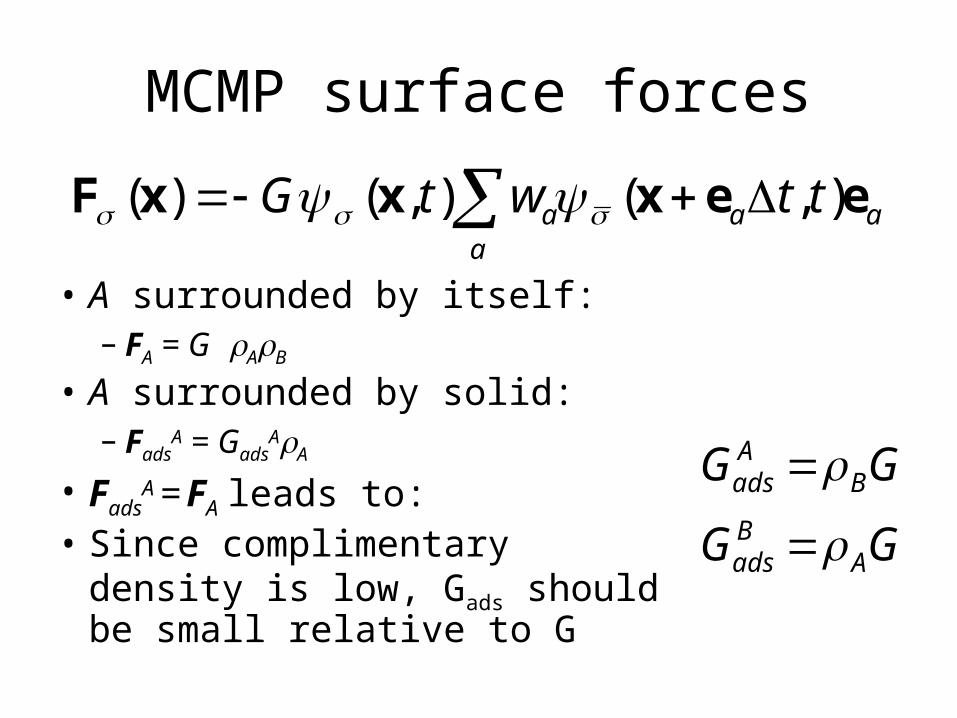
MCMP surface forces

• A surrounded by itself:– FA = G AB

• A surrounded by solid:– Fads

A = GadsAA

• FadsA = FA leads to:

• Since complimentary density is low, Gads should be small relative to G

a

aaa ttwtG eexxxF ),(),()(

GG BAads

GG ABads

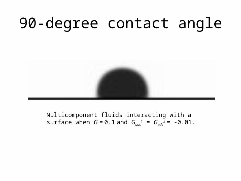
90-degree contact angle

Multicomponent fluids interacting with a surface when G = 0.1 and Gads

1 = Gads2 = -0.01.

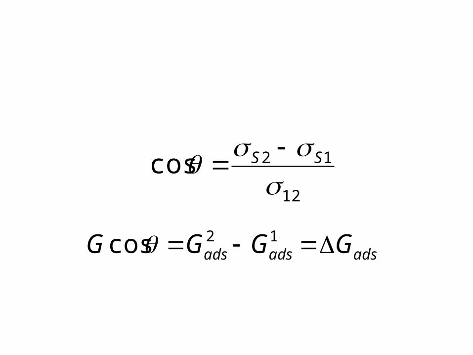
adsadsads GGGG 12cos

12

12cos

SS

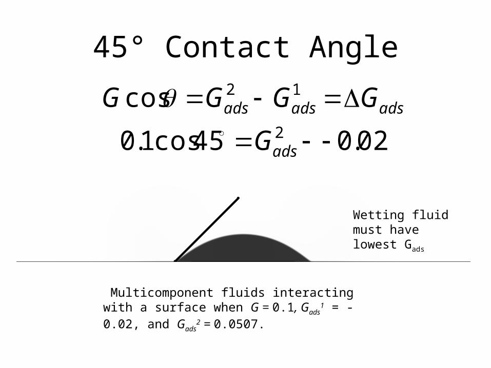
45° Contact Angle

Multicomponent fluids interacting with a surface when G = 0.1, Gads

1 = -0.02, and Gads2 = 0.0507.

adsadsads GGGG 12cos02.045cos1.0 2 adsG

Wetting fluid must have lowest Gads

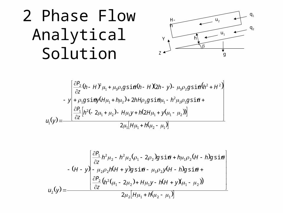
2 Phase Flow Analytical Solution

1211

21112121

122

12211

2221111

22

1 2

22

sinsin2sin

sin2sin

hH

yHhyHhzP

ghghHhHyg

HhgyhHhgHhzP

y

yu

1212

2112122

2122

212122

221

2 2

2

sinsin

sinsin2

hH

yHhyHhz

P

ghHygyHh

ghHhghhz

P

yH

yu

g

q2

q1

u2

u1

h

H-h

Y

Z

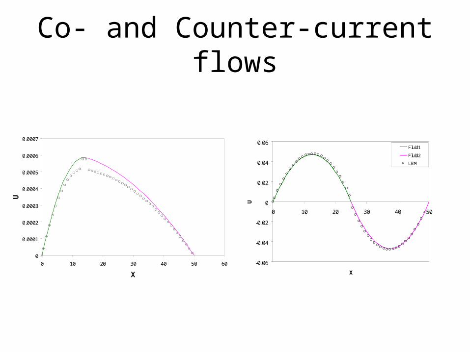
Co- and Counter-current flows

0

0.0001

0.0002

0.0003

0.0004

0.0005

0.0006

0.0007

0 10 20 30 40 50 60

X

U

-0.06

-0.04

-0.02

0

0.02

0.04

0.06

0 10 20 30 40 50

X

U

Fluid1

Fluid2

LBM

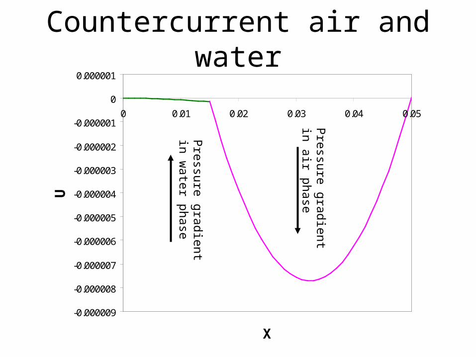
Countercurrent air and water

-0.000009

-0.000008

-0.000007

-0.000006

-0.000005

-0.000004

-0.000003

-0.000002

-0.000001

0

0.000001

0 0.01 0.02 0.03 0.04 0.05

X

U

Pressure gradient in air

phase

Pressure gradient in

water phase

Density and Viscosity Contrasts

• Large density and viscosity contrasts are a major challenge of LBM research.

• McCracken and Abraham (2005): pressure in standard multicomponent LB models is p = (1 + 2)cs

2, where cs is the speed of sound • Significance is that for total pressure to be

constant, the sum of the densities of the 2 species must be constant

• Not the case in real gasses, where differing molecular weights lead to constant pressures despite different densities