MORE FISCAL RESOURCES FOR INFRASTRUCTURE?

EVIDENCE FROM EAST AFRICA1

Cecilia Briceño-Garmendia and Vivien Foster Sustainable Development Department

Africa Region The World Bank

June 28th, 2007

1 We deeply thank peer-reviewers Anand Rajaram, Praveen Kumar, Mohua Mukherjee and Supee Teravaninthorn who kindly provided very valuable comments. We are also grateful to Vishal Agarwal, Sudeshna Banerjee, Daniel Benitez, Mustapha Benmaamar, William Butterfield, Malcolm Cosgrove-Davies, Arnaud Desmarchelier, Antonio Estache, Kene Ezemenari, Katharina Gassner, Paivi Koljonen, Praveen Kumar, Astrid Manroth, Anand Rajaram, Sudhir Shetty, Lars Sondergaard, Maria Vagliasindi, and Stephan Von Klaudy for useful discussions and sharing with us key material that made this paper possible.

1

48086P

ublic

Dis

clos

ure

Aut

horiz

edP

ublic

Dis

clos

ure

Aut

horiz

edP

ublic

Dis

clos

ure

Aut

horiz

edP

ublic

Dis

clos

ure

Aut

horiz

ed

EXECUTIVE SUMMARY Motivation In recent years, there has been a lively debate over the tension between fiscal stabilization and productive public investments in infrastructure. Some economists have argued that the compression of public investment to achieve fiscal stabilization in the late twentieth century was misguided, insofar as infrastructure investments can be growth-enhancing and hence make a positive contribution to the public finances in the longer term. The IMF, however, has questioned whether public investment in infrastructure is really so productive, given endemic inefficiencies as well as the potential for “white elephants”. The debate on allocation and availability of fiscal resources has particular relevance for Sub-Saharan Africa (SSA) facing burgeoning infrastructure needs and meager public budgets. This paper evaluates the extent of fiscal resource availability for infrastructure in four East African countries and explores the main options for its expansion. A number of major channels will be examined. The first is the extent to which expenditure is well allocated across sectors, sub-sectors, expense categories, jurisdictions and geographic areas. The second is the extent to which there is scope for improving efficiency by enhancing the operational performance of SOEs, restoring adequate levels of maintenance, or improving the selection and implementation of investment projects. The third is the extent to which user charges are applied and set at levels consistent with cost recovery. The fourth is the extent to which private sector participation has been fully exploited as a vehicle for raising investment finance. While it is difficult to evaluate these things very precisely, a number of proxy indicators (identified in the table below) are used to shed light on the matter.

Framework for fiscal resource availability Potential channel Basis for evaluation 1) Reallocation of spending Distribution of spending within and outside the budget

Distribution of spending across sectors relative to benchmarks Balance between capital and current spending Distribution of spending across jurisdictions Spatial distribution of spending

2) Higher levels of efficiency a) Operational efficiency Distribution losses (utilities) b) Commercial efficiency Collection losses (utilities) c) Capital efficiency Existence of adequate project screening process

Capital budget execution ratios Average duration of investment projects Maintenance spending relative to technical norms

3) Higher levels of cost recovery Current levels of cost recovery Affordability of subsistence services

4) Greater private finance Current level of private finance relative to benchmarks Availability of public infrastructure with private finance potential Source: Own elaboration

2

Methodology The analysis forms part of the Africa Infrastructure Country Diagnostic, and will eventually be extended to cover an additional 20 countries in Sub-Saharan Africa. It builds on earlier country-specific work on each of the four East African countries (Kenya, Rwanda, Tanzania and Uganda). By pooling together consistently defined fiscal indicators across a number of countries, benchmarking is made possible, and interpretation of the findings is thereby greatly facilitated. The Africa Infrastructure Country Diagnostic is a major knowledge program on the infrastructure sectors in Sub-Saharan Africa that will allow this analysis to be replicated for many other countries on the continent. Given the limitations of IMF data, the paper draws upon an entirely new and customized data collection effort. The IMF Government Finance Statistics are not comprehensive or disaggregated enough to support any analysis of the fiscal costs of infrastructure. Hence, this paper is based on a new standardized cross-country dataset of fiscal indicators that cover both within and beyond the central government budget spending. Private operators are also included to the extent that their assets continue to belong to the state, and/or they continue to be reliant on public subsidies. Data is collected in such a way as to permit both classification and cross-classification by economic and functional categories following the IMF Government Finance Statistics Manual, 2001. Functional categories include the major infrastructure sub-sectors (ICT, irrigation, power, railways, roads, water and sanitation). Economic categories include capital spending, wages and other current expenditures. As far as possible, both budgeted and actual expenditures are recorded for the last three to five years.

The data collection process raised a number of difficult methodological issues, that were dealt with as carefully as possible. First, in many countries it was necessary to recode budget lines so that they are in line with the standardized Government Finance Statistics Manual 2001 functional categories. Second, special care was paid to ensure expenses are analyzed and classified according to their economic use either as capital or current expenditure. Third, it was important to avoid double-counting of transfers from central government to parastatals, special funds and sub-nationals by careful matching-up of the accounts. Notwithstanding these efforts, it is important to be cognizant of the inevitable data limitations in an exercise of this kind. These limitations should be borne in mind when interpreting the results of the analysis. First, since it was not feasible to visit all sub-national entities there is likely under-coverage of decentralized infrastructure expenditures, with particular implications for the water sector. Second, it is not always possible to fully identify which items of the budget are financed by donors, while NGO contributions to rural infrastructure projects are likely to be missed completely. Third, it was not always possible to obtain full financial statements for all the infrastructure special funds that had been identified.

3

Infrastructure Performance East Africa’s infrastructure performance is generally lack-luster when compared against the relevant peer groups. As a result both households and enterprises are seriously under-served. Households have relatively good access to improved water and sanitation, but coverage of electricity is extremely low. Electricity coverage (of little more than 10% on average) lags substantially behind even the already low benchmarks of around 30% for Sub-Saharan Africa and Low Income Countries as a whole. Moreover, the rate of coverage expansion (at 0.6% per year) is also well behind the benchmarks (of around 1.2% per year), suggesting that this gap will only get larger over time. The coverage situation with respect to water (60-70%) and sanitation (40-50%) is much better, with most countries outperforming their peer group. East Africa is also making brisk progress in expanding coverage to improved water sources over time suggesting that this lead will continue, although unfortunately the same cannot be said for sanitation. Enterprise surveys confirm that reliability of power supply is the most severe infrastructure problem from a business perspective. Some 50-80% of manufacturing firms identify it as such, which is well above the average for Low Income Countries as a whole. They report 70-80 days of power outages each year, leading to losses valued at 10-20% of total sales. Transport infrastructure is the next most pressing constraint from a business perspective. Indeed, East African manufacturers report that 2-3% of their cargo is lost in transit, which is about double the average for the Low Income Country peer group. Business dissatisfaction with telecommunications infrastructure is substantially lower than for the other services (5-25%), with the important exception of Kenya (44%). Are Countries Spending Enough on Infrastructure? Current levels of infrastructure spending are high as a percentage of GDP, but remain low in absolute terms. Average annual public spending on infrastructure in East Africa ranges between 5% (Rwanda) and around 10% (Kenya) of GDP, but in general has been converging towards the 6-8% of GDP range. In absolute terms, this amounts to little more than US$20 per capita per year on average. Given both its higher GDP and its larger GDP share devoted to infrastructure, Kenya has by far the largest infrastructure budget in the region. At over US$40 per capita per year this is more than four times the equivalent expenditure in Rwanda. The share of central government spending that is allocated to infrastructure has been rising in recent years, and is now in the 10-20% range. Comparable expenditure figures for middle income countries are at least ten times higher in absolute terms. Relative to middle income countries in Latin America and the Middle East for which comparable data is available, East African countries dedicate on average a slightly higher share of GDP to public spending on infrastructure (7%

4

versus 6%). Nevertheless, given the much higher GDP of the middle income countries, this translates into an absolute level of expenditure that is 10 to 15 times higher. In absolute terms, the level of public infrastructure investment in East Africa amounts to no more than US$7 per capita per year. Within overall public spending on infrastructure, the share devoted to public investment varies enormously across countries. Average annual public investment on infrastructure in East Africa ranges between 2% and 3.5% of GDP. It is striking that although Tanzania and Kenya have by far the highest level of infrastructure spending they also have in comparison the lowest level of public investment in infrastructure. Kenya and Tanzania allocate only about 20% of infrastructure spending on investment. This can be compared with Rwanda and Uganda, which allocate just over half of their infrastructure spending on public investment. This aggregates to a total annual infrastructure investment budget of between US$50 million (Rwanda) and US$220 million (Uganda). Is Infrastructure Spending Well Allocated? It is relevant to ask whether the infrastructure spending envelope is appropriately allocated: across the budget frontier, and between sub-sectors, expense categories, jurisdictions and geographic areas. SOEs account for a high share of total infrastructure spending outside of the budget framework, but fail to meet criteria for sound commercial management. The scope of budget coverage of infrastructure spending follows a broadly similar pattern across East Africa. In most countries, spending by line ministries is on-budget and SOEs are off-budget, while spending by local governments and special funds may be on or off budget depending on the country. At least 50% of total infrastructure spending is channeled through infrastructure SOEs, which control as much as 4-6% of GDP. The majority of capital spending goes through the budget, ranging from around 50% (Kenya, Tanzania) to 90% (Uganda). By contrast, only a minority share of recurrent spending goes through the budget, between 20-30% in most cases. The IMF has developed a number of criteria for determining whether SOEs are run on sufficiently commercial principles to warrant exclusion from the budget. These relate to managerial autonomy, arms length government relations, a level financial playing field and good corporate governance. An evaluation of East African SOEs against these criteria suggest that many of them fall far short; except in cases where extensive forms of private sector participation have been contracted. Sectoral spending allocations appear to be heavily skewed towards the power sector. East African countries are typically allocating 2-4% of GDP on energy, 1.5-2.5% of GDP on transport, and little more than 1% of GDP on water and sanitation. The concentration of expenditure in the power sector (40-60% of the total) is striking given that electricity only reaches 5-20% of the population in these countries, but is likely explained by high oil prices and emergency expenditures associated with the recent power crisis. However, such an arrangement is not sustainable in the long term,

5

nor would it be financially feasible for these countries to substantially scale-up electricity access at such high unit costs of provision. The share of infrastructure spending allocated to investment appears to be too low in most countries, and particularly in the power sector. It is important to preserve an appropriate balance between investment versus operating and maintenance expenditure for infrastructure. Estache 2005 estimates that countries should allocate just over half of their infrastructure spending to investment. Overall, Rwanda is the only country with investment shares high enough to meet this norm. In general, all countries show signs of serious under-investment in the power sector, and potential over-investment in the water sector. The picture for the transport sector is mixed. The share of spending going to capital differs even more dramatically across institutional category than it does across sector. In most cases, Central Government agencies allocate 75-95% of their infrastructure spend to capital, compared with 15-20% of the spending for SOEs. While shares of wage spending do not appear to be unreasonable, many countries and sectors show abnormally high shares of non-wage current spending. Across East Africa there is a recent tendency to decentralize public service responsibilities and associated government spending towards local jurisdictions. Kenya and Tanzania are the two countries that have gone furthest in fiscal decentralization to date, and in both countries local governments rely predominantly on untied fiscal transfers. Estimated infrastructure spending by local governments in these countries have been growing exponentially (at around 50% per annum) but from very different baselines. Thus, at present, local government spending on infrastructure in Kenya at around 1.5% of GDP is higher than the equivalent share in Tanzania (at 1% of GDP) (Figure 9). In Rwanda and Uganda, transfer of resources to local jurisdictions is predominantly through tied funds such as the Community Development Fund (Rwanda) or the Poverty Action Fund (Uganda). These transfers amount to 0.4% of GDP for Rwanda and about 1.3% of GDP in Uganda. It is estimated that rural areas benefit from 20-30% of infrastructure spending, whereas they account for 75-85% of the population. While no precise information is available, a very rough estimate of the share of public spending on infrastructure that benefits rural areas can be made. The estimate suggests that rural infrastructure spending typically amounts to 1-2% of GDP, equivalent to US$3-9 per capita per year. The share of infrastructure spending going to rural areas is thus much lower than their share of total population. While certainly inequitable at the first sight, this likely reflects the fact that urban areas tend to account for the bulk of the economic activity, and in that sense have a stronger demand for infrastructure services, as well as the resource base to support them. Furthermore, a deeper equity analysis should take into account unit cost and population density variables. Nevertheless, to the extent that rural infrastructure is a key platform for growth in agricultural productivity, this is potentially a concern.

6

How Efficient is Infrastructure Spending? The next question relates to the efficiency with which the different institutions use the infrastructure resources allocated to them. Central government, SOEs and special funds are considered in turn. Central government appears to suffer from serious inefficiencies in the implementation of capital projects. The key finding is that only 50-60% of capital budgets can be executed within the one year budgetary cycle. This is ratio is fairly consistent across countries and sectors; although Kenya is the worst offender with a capital budget execution ratio of only 33%. The under-spend on capital investment can be contrasted with a tendency to over-run budget allocations with regard to current expenditure, and there may be a connection between the two. Since investment projects are rarely completed in a single year, it is relevant to look at the track record on project implementation. The only available evidence, from Kenya, suggests that domestically finance investment projects take more than four years on average to complete. Together, these findings suggest that the central government faces real difficulties in converting public investment into productive infrastructure assets. SOE inefficiency is also a material problem at the macro-economic level, particularly in the energy sector and particularly in Tanzania. Inefficient SOEs impose a variety of hidden costs on the economy as a result of under-pricing, inefficient revenue collection and distribution losses. There are a number of ways in which these can be quantified. The evidence suggests that these costs are large relative to the economic scale of the SOEs themselves, accounting for 30-80% of their total revenues. In GDP terms, the hidden financial costs of water utilities look relatively small (less than 0.1% of GDP). However the hidden costs of power utilities can be much larger (0.2-0.4% of GDP), and in the exceptional case of TANESCO can be as high as 1.5% of GDP. The main source of the inefficiency differs substantially from one case to another, and the level of hidden costs can also move quite quickly in response to policy and management changes. Leaving aside the more political issue of under-pricing, the potential dividend from simply improving the operational efficiency of SOEs, ranges between 0.5-0.8% of GDP. The problem of under-pricing by TANESCO is itself worth 1.3% of Tanzania’s GDP. Road funds functioning in most countries have the potential to adequately fund road maintenance, but face difficulties with revenue collection. In recent years, East African countries have created a variety of special funds to support infrastructure development. These include road maintenance funds, sub-national funds, and rural infrastructure funds. Together they absorb no more than 0.5% of GDP, almost all of it current expenditure. Most countries have established road funds aimed at safeguarding revenues for maintenance by capturing a variety of road user charges, such as petroleum levies. In most cases, the revenue base of the road funds is potentially large enough to provide adequate levels of funding for road maintenance. The situation in Kenya is relatively good. However, both in Rwanda and Tanzania road funds face major difficulties with revenue collection. The situation is particularly serious in

7

Rwanda where the road fund is only capturing resources adequate to maintain 20% of the network in good condition, and where in any case 80% of the network is in need of rehabilitation. There is urgent need for greater transparency and predictability of project selection and prioritization of investment. The lack of (i) clear criteria for evaluation of projects and (ii) clear attribution of responsibilities for carrying out economic project evaluation and portfolio gate-keeping; is hampering the impact that investment of admittedly scarce resources could have. Furthermore, systematic investment planning is a pre-requisite for engaging the private sector in a more permanent and onerous manner. Is There Additional Scope for Cost Recovery? Most SOEs comfortably cover their operating costs, but nearly all of them fall well short of covering likely capital costs. Operating cost recovery ratios range from 80% to over 300%, although in the majority of cases they are close to 100%. Given unreliable depreciation charges and virtually non-existent investment programs, it is not possible to get reliable estimates of total capital costs from the company accounts. As a simple benchmark, it is assumed that SOEs would need to recover twice their operating costs in order to be self-sufficient in capital expenditure. Only one or two of them meet this goal; the vast majority would need to double their operating revenues in order to do so. SOE customers are overwhelmingly drawn from the upper end of the wealth distribution, but nonetheless cannot be considered wealthy. In order to assess the social and political feasibility of such a large increase in cost recovery, the distributional incidence of household connections is examined together with information about the purchasing power of the households. The analysis shows that between 70-95% of water and electricity connections belong to households in the top quintile of the wealth distribution, and that virtually no households in the bottom half of the distribution have access. This suggests that existing subsidies to the utility sector are extremely regressive in their incidence; with a very high concentration coefficient of around 0.75. Nevertheless, on closer examination even these wealthier households live on family budgets of no more than US$240 per month. If a standard affordability threshold of 5% of income is considered, this means that they have no more than US$12 per month to spend on any particular utility service. Thus, while distributionally progressive, major tariff increases may nonetheless be socially difficult to implement. Are External Resources Adequately Mobilized? On average, East African countries raised 3.2% of GDP in external finance for infrastructure. The total ranges from 2.4% of GDP (Rwanda) to 3.8% of GDP (Tanzania). With the exception of Kenya that relies predominantly on private finance, donors accounted for 70-80% of the external finance raised for infrastructure. In the case of telecommunications, more than 90% of external finance is provided by the

8

private sector. In the case of transport and water and sanitation, more than 95% of the external finance is provided by donors. In the case of energy, the balance between private and donor finance varies substantially across countries. Most countries in East Africa have raised significantly more private finance for infrastructure than their peers. Whereas the benchmarks for LIC and SSA countries are less than 1% of GDP in private finance for infrastructure, all of the East African countries (with the exception of Rwanda) raised between 1-2% of GDP. Most countries in the region have made major strides in divesting telecom incumbents, licensing entry of new mobile operators, awarding concessions for railways, as well as some ports and airports, using management contracts for the major power and water utilities, and allowing Independent Power Producers. Nevertheless, private participation has not come without substantial mobilization of fiscal resources of its own. In particular, payments to Independent Power Producers under Power Purchase Agreements in Kenya and Tanzania absorb around 1% of GDP and account for 40% of power spending, even though the associated plant represents only 20% (Kenya) to 40% (Tanzania) of the national generation portfolio. Potential for freeing fiscal resources by attracting additional private finance appears limited, except in the case of Kenya. Kenya still has to divest its telecom incumbent and has a significant pipeline of projects suitable for concession or BOT such as a number of new thermal power projects, the Eldoret-Kampala oil pipeline, the electricity interconnection Tanzania-Kenya, the Nairobi urban toll road, the remainder of the Mombasa port, the passenger terminal at Nairobi airport and the Kenya-Sudan railway project. To a lesser degree opportunities for concessions or BOTs are present in Rwanda (Lake Kivu Gas Development and power project) and Tanzania (electricity interconnection with Zambia, management of cargo port terminal and the development of the central transport corridor). Most countries in East Africa have also raised significantly more donor finance for infrastructure than their peers. Whereas the benchmarks for LIC and SSA countries are around 1% of GDP in private finance for infrastructure, all of the East African countries (with the exception of Kenya) raised between 2-3% of GDP. Estimates suggest that donor finance contributed approximately 50% to public investment on average, the residual being domestically financed. Across all countries, the transport sector is consistently the most reliant on donor finance for investment (with the reliance ranging from 40-80%), and moreover absorbs the largest share of overall donor finance (between a half and two thirds of the total). However, these figures are likely to be under-estimates given that the specific components of public investment that are funded by donors are not always clearly identified in the budget. As a result, it is difficult to make very precise estimates of the residual, which is the domestically financed share of public investment. Nevertheless, the limited evidence available suggests that domestic resources appear to be making a substantial contribution.

9

Country Specific Issues. Kenya spends a large share of GDP on infrastructure but converts barely 20% of it into public investment due to budget execution problems. Not only does the country present the highest level of infrastructure spending (even excluding all expenditure by water utilities that could not be captured in this study), but is also has the one the lowest level of public investment at about 2% of GDP (managing to invest less in per capita terms than Rwanda that devotes only half as much of its national resources to infrastructure spending). High spending by Kenyan SOEs merits closer scrutiny, particularly in the energy sector. The SOEs control a particularly large share of public expenditure in Kenya, amounting to 4-6% of GDP (even excluding the water utilities) and likely deserve closer budgetary scrutiny. Spending on energy up to 2005 was very high at 3.7% of GDP. Recent efficiency improvements in KPLC have brought about gains of around 0.8% of GDP, although there is still further scope for improvement under new private management. Rwanda’s main problem is the low level of infrastructure spending, given its weak infrastructure endowment, particularly with respect to roads. Rwanda presents some of the weakest infrastructure performance indicators in the region, particularly with regard to power (with coverage of only 6%) and roads (with only 20% of the network in reasonable condition). In spite of this Rwanda spends less than 5% of GDP on infrastructure, or little more than half the benchmark level of 9%. Furthermore, there is some evidence that Rwanda allocates a relatively low share of its overall budget to infrastructure and that it spends its current resource envelope relatively well. While there is always room for improvement, Electrogaz (the main SOE providing both energy and water services) looks relatively efficient alongside other utilities in the region. At the same time, Rwanda manages to invest a much higher proportion of its infrastructure resources (around 50%) than the other East African states (around 30% on average) tough mostly through the budget. Finally, the lack of funds available for road maintenance due to delayed payment of revenues owing to the Road Fund is a particularly major cause for concern, as it will lead to further deterioration of a network that is already in critical condition. In Tanzania, the power sector gives the greatest cause for concern. The large quasi-fiscal deficit associated with TANESCO (amounting to an estimated 1.8% of GDP) is probably the single most salient feature of the fiscal analysis for Tanzania. Since the bulk of the deficit is related to under-pricing the solution may not be politically straightforward. A second major concern is that – similar to Kenya – Tanzania only converts a small proportion of its infrastructure spending to investment (20%), and presents a low capital budget execution ratio (60%). On the other hand, the roads sector stands out as one where Tanzania is performing comparatively well with 84% of the network in reasonable condition. However, the evasion of the fuel levy is a serious problem that needs to be addressed in order to safeguard an adequate revenue flow to the Road Fund.

10

A similar story can be told about Uganda. While the quasi-fiscal deficit of Uganda’s power utilities is very much lower than in Tanzania due to better pricing practices, their operational performance is actually worse: distribution and collection losses absorb 0.7% of GDP. The fact that the power sector absorbs 60% of public infrastructure spending in Uganda is evidently a major concern, particularly given the very limited levels of investment to date. Uganda presents a good balance between investment and operating and maintenance expenditure, in spite of a low capital budget execution ratio. However, its overall level of spending may be on the low side, particularly in what concerns electricity distribution network and the recently privatized railways company.

11

TABLE OF CONTENTS 1. Motivation 2. Methodology 3. Infrastructure Performance 4. Are Countries Spending Enough on Infrastructure? 5. Is Infrastructure Spending Well Allocated? (a) Allocation across budget categories (b) Allocation across infrastructure sub-sectors (c) Allocation across expense categories (d) Sub-national allocation (e) Spatial allocation 6. How Efficient is Infrastructure Spending? (a) Central Government (b) State Owned Enterprises (c) Special Funds 7. Is There Additional Scope for Cost Recovery? 8. Are External Resources Adequately Mobilized? (a) Private finance (b) Donor finance 9. Conclusions on Availability of Additional Fiscal Resources for Infrastructure Annexes Data Annexes

12

1. MOTIVATION Since the early 2000s, there has been a lively debate over the tension between fiscal stabilization and productive public investments in infrastructure. Easterly and Serven (2003) first drew attention to the fact that fiscal stabilization programs supported by the International Monetary Fund (IMF) during the 1980s and 1990s in Latin America had to a large extent been accommodated through a compression of productive public investments, notably in infrastructure. They argued that this approach was misguided, insofar as infrastructure investments can be growth-enhancing and hence make a positive contribution to the public finances in the longer term. The authors therefore proposed a shift away from the short-term preoccupation with fiscal deficits, towards a longer term focus on fiscal solvency. At around the same time, Blanchard and Giavazzi (2003) advanced a similar argument with respect to the European Union’s Stability and Growth Pact, which limited budget deficits to 3% of GDP and formed the macro-economic underpinning of European Monetary Union. The IMF questioned the assumption that public infrastructure spending in developing countries was necessarily growth-enhancing. In its 2004 review of the issue, the IMF raised concerns about screening procedures for capital projects (and hence the potential for “white elephants”) and more generally about the limited efficiency of public spending on infrastructure (IMF, 2004a). The IMF also highlighted the potential for abuse of Public Private Partnerships as a means of freeing fiscal resources in the short term, at the cost of locking them in the longer term while creating contingent liabilities for the state (IMF, 2004b). Overall, the IMF concluded that efforts to make more fiscal resources available for infrastructure should focus on reprioritization of spending within the current fiscal envelope, and possible exclusion of commercially-run state-owned enterprises from the budget envelope in some countries. The debate on allocation and availability of fiscal resources has particular relevance for Sub-Saharan Africa (SSA) facing burgeoning infrastructure needs and meager public budgets. Estache 2005 estimates that SSA’s infrastructure investment needs amount to US$22 billion per year, which is around double what has historically been provided by a combination of public expenditure, overseas development assistance and private sector finance. In addition, a further US$17 billion per year would be needed to operate and maintain SSA’s infrastructure, which again is more than twice what has historically been provided through cost recovery, public expenditure and overseas development assistance combined. At the same time, based on limited historical data, Estache estimates that central government spending on infrastructure declined from 4.2% of GDP in the early 1980s to 1.6% by the late 1990s. Over the same period, central government allocations to health (around 2% of GDP) and education (4-5% of GDP) remained relatively constant. Estache infers from this finding that infrastructure spending may have borne the brunt of fiscal compression during the 1990s. Nevertheless, recent evidence suggests that the case for additional infrastructure investment is not always clear even in a dynamic framework. In a recent paper,

13

Estache and Muñoz (2007) modify the IMF’s financial programming framework to incorporate the potential dynamic growth-enhancing effects of public investment. They calibrate the model using macro-data for Uganda and Senegal. In the case of Uganda, they find that new infrastructure investment is output-enhancing but due to low productivity worsens the debt to GDP ratio. In the case of Senegal there is no evidence that new infrastructure investment is output-enhancing. Nevertheless, in both cases, increasing resources to infrastructure maintenance or to new investments in health and education are found to have better dynamic effects than increasing investment in new infrastructure. There is not a clear cut criterion to judge the quality of public spending across sectors and empirical assessments are severely limited due to data availability. A recent paper by Estache et al. (2006) weakly suggests that when compared with health and education, infrastructure sectors -- particularly transport— have the largest potential for increasing returns on investment within the existing resource envelope. Some efficiency gains would naturally materialize when long-life assets –designed at construction based on 20-30 year demand projections and with low-returns early in project life— start ageing and reaching higher marginal returns. Other efficiency gains would depend on the successful implementation of policy decisions aiming at (i) a more efficient execution of multiyear projects to ensure cost are kept to the minimum and countries seize soonest the benefits of large-multiyear investments, and (ii) making sure than periodic maintenance of relatively under utilized assets (such as new roads) are not postponed. Estache et al. are, however, severely limited by the availability and quality of data, particularly of that on public expenditure admittedly sparse and of poor sector-level coverage. Infrastructure presents a number of characteristics that complicate its treatment in the public finances. On the one hand, infrastructure investments are large, lumpy and infrequent, and often take more than one budget cycle to complete. This makes infrastructure investments hard to accommodate within a single budgetary cycle, and much better suited to a medium-term expenditure framework. It also raises the risk that budget allocations for multi-year investment projects are not sustained over time. At best, this can severely delay the implementation of projects reducing their eventual rate of return. At worst, it may leave a country with a graveyard of incomplete public works that never materialize into a productive infrastructure asset. On the other hand, infrastructure assets require a sustained preventive maintenance program. Failure to maintain eventually leads to total asset deterioration necessitating major rehabilitation investments that cost considerably more in present value terms than the maintenance spending that would have prevented them. Nevertheless, deterioration is a gradual process, and maintenance has low visibility, creating a permanent temptation to defer such spending to accommodate more politically-rewarding expenditures. There are a number of different ways in which additional fiscal resources can be made available for infrastructure financing. Subsequently, the World Bank has developed its own framework for evaluating the extent of the availability of fiscal resources in particular country contexts (World Bank, 2006, 2007). The four options

14

identified are raising additional tax revenues, increasing public sector borrowing, capturing more international aid, and improving the efficiency of current expenditure. Ultimately, these boil down to three strategies: securing more resources whether from local tax payers or foreign tax payers (in the form of grant aid), bringing forward future resources by borrowing either from the markets or from development institutions, and using current resources more efficiently. It is important to mention that efficiency relates both to the way in which current resources are allocated, which should be to their highest value use, and to the way in which they are spent, which should be as cost-effectively as possible. The same general framework can be readily applied to the infrastructure sectors. It points to a particular approach for evaluating the extent of the availability of fiscal resources and identifying options for its expansion. First, there is always the possibility of reallocating expenditure across sectors and sub-sectors. Such reallocation can take place either across infrastructure and non-infrastructure sectors, or between different sub-sectors within infrastructure. It is not straightforward to assess the scope for reallocation across sectors. Cross-country benchmarking can sometimes help to identify outliers with expenditure patterns that seem overly skewed in one direction or another. However, otherwise a great deal of subjective judgment is in assessing the suitability of spending allocations across sectors. Assessing allocations across infrastructure sub-sectors may be a little more tractable. By benchmarking the relationship between spending levels and sector outcomes across countries, it may be possible to identify evident cases of over or under-spending. Nevertheless, the long-lived nature of infrastructure assets, make it difficult to make reliable connections between spending and outcomes over relatively short periods of time. Second, there are various ways in which the efficiency of infrastructure spending can be improved. Infrastructure parastatals tend to suffer from various endemic forms of operational inefficiency including high distribution losses (in power and water), and low collection of revenues from user charges. These can be quite readily assessed by benchmarking standard utility performance parameters. When it comes to capital expenditure, a more complex series of issues arise. First, inefficiencies may arise in the project selection process, if white elephants are allowed to be built. Second, inefficiencies may arise in the implementation process if construction costs escalate due to limited competition, weak governance, or inadequate budget allocations that impede the timely completion of investment projects sometimes leaving them in a state of limbo for many years. Third, inefficiencies may arise over the life of the capital asset. Maintenance of infrastructure is often under-funded, leading to rapid deterioration and necessitating frequent rehabilitation of assets that is much more costly in present value terms than a sound preventive maintenance program. An in-depth assessment of the efficiency of infrastructure spending would demand a level of detailed data collection and analysis that lies beyond the scope of this report. However, some simple diagnostic tests can be undertaken that help to identify where the largest problems may exist. These include a qualitative assessment of project screening procedures, an examination

15

of capital budget execution ratios, and a comparison of maintenance expenditures against technical norms. Occasionally, it is also possible to analyze the portfolio of active investment projects in order to detect whether budget allocations over time are allowing projects to be completed in a timely fashion. Third, many infrastructure services operate with some degree of cost recovery. Therefore, increasing user charges is one clear policy option for increasing the availability of fiscal resources. Nevertheless, there may be political barriers or affordability constraints that in practice limit the feasibility of doing this. In evaluating the scope for increasing the availability of fiscal resources through this route, it is therefore of interest to evaluate both the existing extent of cost recovery, and the scope for further increases in cost recovery given local political and social sensitivities. Last but not least, there is scope for private sector finance in some areas of infrastructure. Since the late 1990s, a number of Sub-Saharan African countries have had some success in raising private finance for traditionally state-funded infrastructures, amounting to 0.8% of GDP per year on average in recent years. The scale of private finance has not been as large as originally anticipated, and it has tended to focus on more lucrative areas of infrastructure (such as telecommunications, power generation, railways and ports) as well as in the larger and wealthier economies (such as South Africa, Nigeria and Kenya). Nevertheless, within these limited areas it can make a very significant contribution if for nothing else to relieve the fiscal burden. In terms of freeing fiscal resources in the short run, it is important to understand the effect of private finance, which is merely to provide access to an alternative source of capital. Private financiers must ultimately be repaid, either through user charges (in which case their participation is premised on prior achievement of cost recovery) or through government subsidies. What perhaps is fundamental is that private finance may make fiscal resources available by introducing a higher level of efficiency in the use of resources through better management, although this may come at the expense of a relatively high cost of capital. The extent of fiscal resources that can be freed for other uses by increased private sector finance can be roughly gauged by benchmarking the extent of private participation to date, and identifying potentially lucrative components of infrastructure that may remain in public hands.

16

Table 1: Framework for evaluating fiscal resource availability Potential channel Basis for evaluation 1) Reallocation of spending Distribution of spending within and outside the budget

Distribution of spending across sectors relative to benchmarks Balance between capital and current spending Distribution of spending across jurisdictions Spatial distribution of spending

2) Higher levels of efficiency a) Operational efficiency Distribution losses (utilities) b) Commercial efficiency Collection losses (utilities) c) Capital efficiency Existence of adequate project screening process

Capital budget execution ratios Average duration of investment projects Maintenance spending relative to technical norms

3) Higher levels of cost recovery Current levels of cost recovery Affordability of subsistence services

4) Greater private finance Current level of private finance relative to benchmarks Availability of public infrastructure with private finance potential Source: Own elaboration

The objective of this study is to evaluate the extent of fiscal resource availability for infrastructure in four East African countries: Kenya, Tanzania, Rwanda and Uganda. All four countries face major infrastructure needs and limited financial resources, making the question of availability of fiscal resources for infrastructure a particularly pressing one. Following introductory sections that motivate the analysis, explain the methodology and provide the general infrastructure context for the region, the remainder of the report is structured around a series of questions related to the evaluation of fiscal resource availability described above. Thus, Section 4 asks whether countries are spending enough on infrastructure. Section 5 questions whether infrastructure spending is appropriately allocated across budgetary categories, infrastructure sub-sectors, expense categories, jurisdictions and geographical areas. Section 6 asks whether infrastructure spending is efficient. Section 7 takes-up the question of cost recovery. Section 8 examines whether countries are raising adequate levels of external finance. The final section returns to the conceptual framework outlined above and tries to reach some conclusions on the extent of additional fiscal resource availability.

17

2. METHODOLOGY The International Monetary Fund’s (IMF) Government Finance Statistics (GFS) do not provide a detailed or comprehensive picture of infrastructure spending. At present, the GFS constitutes the main source of cross-country data on public finance. However, it presents a number of problems from an infrastructure perspective particularly for Africa, where data availability is by comparison to other regions more limited. On the one hand, the GFS focuses on tracking general government expenditure, whereas a large share of infrastructure spending is through non-financial public corporations (parastatals). Moreover, even within the expenditure tracking of the general government, GFS is greatly limited in practice to central government expenditure, scarcely reporting sub-national and special funds, two other important channels of infrastructure spending.2 On the other hand, the GFS does not provide for a very detailed breakdown by specific infrastructure sectors, and expense categories within each sector. In response to the gap, this study builds-up a novel database of standardized cross-country data that gives a comprehensive picture of infrastructure spending. The analysis presented in this report is based on a systematic cross-country data collection process that aims to capture as comprehensive a picture as possible of public expenditure on the infrastructure sectors both within and beyond the central government budget. The data collection process is based on a standardized methodology that is developed and explained in some detail by Briceño-Garmendia (2007). In order to ensure a consistent methodological approach that supports cross-country comparability of the data, the methodology includes detailed templates that guide the data collection process in the field. The data collection and fiscal analysis in East Africa was undertaken as an initial pilot phase for the AICD study, to be extended to other parts of Africa. The Africa Infrastructure Country Diagnostic is a much broader knowledge program aimed at achieving a substantial improvement of our knowledge base for the infrastructure sectors in Sub-Saharan Africa. The AICD focuses on documenting public expenditure, investment needs and sector performance across five major infrastructure sectors (energy, ICT, irrigation, power, transport) in 24 focus countries. The analysis presented here develops the public expenditure analysis for the four pilot countries in East Africa, and will shortly be extended to cover the additional 20 Sub-Saharan African countries covered under the AICD. This paper pools the results of more detailed work in each of the four countries, benchmarks them against each other, and performs additional analysis. The four

2 Based on the IMF (2001), the public sector can be roughly divided into general government and public corporations. General government comprises central, state and local governments. Public corporations can be grouped, according to the nature of their activities, into financial corporations (engaged in providing financial services for the market) and non-financial corporations, (engaged in producing goods and non-financial services).

18

East African countries were chosen as pilots because of country level demand for the analysis to support on-going economic and sector work. In the case of Kenya, Rwanda and Uganda, this work fed into the respective 2006/07 Country Economic Memorandums. In the case of Tanzania, the work formed part of the 2006/7 Public Expenditure Reviews. This report therefore draws extensively on the set of four original country-specific fiscal analysis reports (Briceño-Garmendia, 2006; Briceño-Garmendia and Butterfield, 2006; Gassner, 2006; and von Klaudy and Benitez, 2006). By standardizing and pooling together the results of each of the country studies, this paper provides a more informative overview of the East African fiscal situation for infrastructure and permits benchmarking to facilitate the interpretation of the findings. The methodology aims to be comprehensive in the sense of covering all relevant budgetary and non-budgetary areas of infrastructure spending. The collection of data on fiscal spending was grounded in an overview of the institutional framework for delivering infrastructure services in each of the countries. This aimed to identify all the different channels through which public expenditure on infrastructure takes place. The work began with a detailed review of the central government budget. Thereafter, financial statements were collected from all the parastatals and special funds that had been identified in the institutional review. In countries where infrastructure service providers are highly decentralized (e.g. municipal water utilities), it was only possible to collect financial statements from the three largest service providers. Privatized infrastructure service providers were included to the extent that they remain majority government owned, or they continue to depend on the state for capital or operating subsidies. Thus, telecommunications incumbents are typically included, whereas mobile operators are not. In some countries, local governments have begun to play an increasing role in infrastructure service provision. It was not possible to collect comprehensive expenditure data at the local government level. However, in some cases the central government produces consolidated local government accounts. Where these do not exist, an alternative source of information are the fiscal transfers from central to local governments, which are reported in the budget and on which local governments rely heavily given limited alternative sources of revenue. In some cases, transfers are earmarked for infrastructure-related spending, whereas in others the share allocated to infrastructure could only be estimated. Data is collected in such a way as to permit both classification and cross-classification by economic and functional categories. That is to say that a matrix is established so that spending on each functional category can be decomposed according to the economic nature of the expense and vice versa. Functional classification follows as closely as possible the four-digit category of the IMF’s Government Financial Statistics Manual 2001 (IMF, 2001) and allows the identification of all the major infrastructure sub-sectors.3 The economic classification of expenses also follows the IMF’s Government Finance Statistics Manual 2001 framework. This permits a

3 Based on the IMF Classification of Functions of Government, the main categories covered in the study are Electricity (0435), Road Transport (0451), Water Transport (0452), Railway Transport (0453), Air Transport (0454), Pipeline & Other Transport (0455), Communication (0460), Waste Water Management (0520) and Water Supply (0630). Irrigation spending is estimated as a share of Agriculture (0421).

19

distinction between current expenditures and capital expenditures, and various sub-categories thereof.4

As far as possible, both budget estimates and actual expenditures are recorded for the last three to five years. There are commonly three different stages in the public expenditure process. First, resources are budgeted for particular purposes, then funds are released from the Ministry of Finance to the responsible institutions, and finally resources are actually spent by the recipient institutions. Expenditure patterns can differ substantially across these three different stages. While actual spending is the ultimate variable of interest, and the main focus of the results presented in this report, it is also important to understand how infrastructure spending is affected by the budget execution process. To this end, both budgeted and actual expenditures are recorded wherever possible. Attempts were also made to capture release figures, however with only very limited success.

The data collection effort raised a number of difficult methodological issues. First, in many countries it is necessary to recode budget lines so that they are in line with the standardized GFSM 2001 functional classification. Having expenses coded according to the same functional classification is a pre-requisite not only for analyzing spending trends over time but also for allowing meaningful comparison of spending patterns across countries. Many countries have not yet adopted the GFSM2001 standards and hence do not necessarily use the functional codes described above. Hence, in some cases it was necessary to do a line by line recoding of the budget in consultation with the corresponding line ministries. Functional areas can be spread across many institutions and are subject to reallocation from one institution to another contingent to changes in institutional responsibilities and institutional frameworks over time. As a way of example, it is not unusual that expenses on the GFSM 4-digit function water supply (0630) can be carried out simultaneously by the Ministry of Works, the Ministry of Water and Sanitation, and/or the Ministry of Local Governments, at one specific year, while at the following year a public sector restructuring brings all these ministries together under the same umbrella with different institutional codes. If budget lines are coded exclusively according to institutions, monitoring of functional expenses over time would be only possible if departments and institutions remain static over the period under analysis. Furthermore, as there are no two single countries sharing exactly the same institutional layout, recoding expenses as to match a common functional classification is the only way of producing meaningful cross-country comparison.

4 Current expenditures to be broken down into compensation of employees, use of goods and services, consumption of fixed capital, interest, subsidies, grants and transfers, social benefits, and other current expenditure. Capital expenditures can be broken down into “buildings, structures, machinery and equipment”, other fixed assets, other capital expenditure, and transfers of capital expenditures to lower levels of government.

20

Second, there is great difficulty of ensuring that expenses are analyzed and classified according to their economic use. On the one hand, there is not a clear cut separation between what should be considered capital as supposed to rehabilitation or even maintenance expense. As much as possible, the data collection was framed by a clear remapping between the economic classification used in the country and the GFSM2001 economic classification to develop a common understanding across countries. On the other hand, capital and current expenditures can be buried ambiguously under budget categories simply by mistake due to ambiguities in the nature of the expenditure but also there may be budgetary incentives for deliberate misclassification in order to increase the chances of budgetary approval.5

Great care was taken during the data collection process not to take budget lines within the development and recurrent budgets at face value. Dual budgeting is not uncommon in Africa. During the first years of independence, many African countries split their budgets into development and recurrent budgets under the premise that capital spending (to be primarily accounted under development budgets) is more productive than current spending (primarily accounted under recurrent budgets). In practice, development budget items started to have higher priority and less restrictive requirements to entry. By contrast, discretionary components of current spending faced more severe controls. Further on the road, stand-alone development budgets were supported by Donors, who saw in them a means for ring-fencing resources to specific projects. Agencies started to disguise current expenses as capital in order to secure resources and have access to external funding. In any case, the misclassification may happen regardless of these incentives. Inevitably, Donor funded-projects have current spending elements and increasingly include provisions for allocating funds to maintenance. Each vote was individually examined and assigned to the correct capital or current expenditure category. As a result, it is possible, among other things, to quantify the extent to which misclassification of spending across budget categories has been taking place in the East African countries under study (see Box 1 below). It becomes evident that nowadays, development budgets are a lousy proxy for investment and the functional separation between the two is increasingly fuzzy. For infrastructure sectors, the separation of budgets is creating coordination problems between investments and the planning and programming of maintenance streams generated by them. This reinforces the temptation for postponing (or not even executing) maintenance of existing assets and delaying allocation of resource of ongoing projects. This situation per se makes monitoring of the quality of spending an uphill task.

5 Unfortunately the GFMS2001 leaves many of economic categorizations open to interpretation, particularly in what concerns the uses of expenses most relevant to infrastructure services (eg rehabilitation, operations, and maintenance). In this first report, the analysis will be constrained to establishing the broad distinctions between current and capital

21

Box 1: Evidence of misclassification of expenditures across budget types The four countries in study have dual budgets aiming at separating capital expenses –in principle recorded in the development budget— and current expenses –in principle recorded in the recurrent budget. The data collection process took great care to examine whether individual budget lines were correctly classified according to their economic nature into capital versus current spending; regardless of whether the budget line belonged originally to either budget. The exercise showed that between 6% and 12% of expenditure was misclassified (see chart below). There was a very clear systematic bias towards one or other direction of misclassification in each country. This finding suggests that misclassification reflects behavioral incentives, rather than random errors. The direction of the misclassification differed substantially across countries. For Kenya and Uganda, it is a case of current spending masked in the development budget likely responding to incentives created by less flexible criteria for allocating discretionary shares of the recurrent budget than for shares of the development budget. For Rwanda and Tanzania, it is a case of misclassifying capital spending within the recurrent budget. This situation might be explained by the observed characterization of rehabilitation spending as maintenance rather than as investment.

0%

2%

4%

6%

8%

10%

12%

14%

Kenya

Rwanda

Tanza

nia

Uganda

Per

cent

age

of to

tal i

nfra

stru

ctur

e sp

endi

ng

Capitalmisclassified asRecurrentBudget

Currentmisclassified asDevelopmentBudget

Source: Africa Infrastructure Country Diagnostic, 2007

Third, care must be taken to avoid double counting of transfers between different parts of the government. Transfers from central government to parastatals, special funds and sub-national governments are potentially reported twice: once as a central government transfer, and once as expenditure by the recipient institution. Great care was taken to match-up these line items across institutions and ensure that they were counted only once, as expenditure by the recipient institution. Notwithstanding these efforts, it is important to be cognizant of the inevitable data limitations in an exercise of this kind. These limitations should be borne in mind when interpreting the results of the analysis. First, there is likely under-coverage of decentralized infrastructure expenditures, with particular implications for the water sector. The study does not adequately capture spending by small decentralized service providers (e.g. municipal water

22

utilities), or spending by local governments that is not funded through fiscal transfers. This concern does not affect countries with highly centralized administrations and/or national water utilities (e.g. Rwanda, Uganda). Even in more decentralized countries, it is known that locally generated revenues are small, and that the share of total utility customers served by providers in small municipalities is relatively low. In the case of Tanzania, only data for the three largest water utilities were captures. Unfortunately, in the case of Kenya, due to recent sector reforms it was not possible to obtain financial statements from any water utilities. Hence, the Kenya data substantially understates the extent of water expenditure. Second, there are some difficulties in fully identifying external finance through the budget. Expenditure items that depend on external funding from donors are not routinely identified as such in the budget, making it difficult to reliably estimate the relative contribution of Overseas Development Assistance. One reason for this may be the fact funding for budget items relating to donor projects is often a blend of domestic and external resources. Beyond official overseas development assistance, resources channeled through Non-Governmental Organizations to support small-scale infrastructure projects in rural communities are also very difficult to capture through central government channels. Third, it was not always possible to obtain full financial statements for infrastructure special funds. The level of transparency and accountability for the spending of infrastructure special funds was found to be highly variable across countries and sectors. In a significant number of cases, it was not possible to obtain financial statements for these funds. This was a particular problem in the case of Uganda. However, it should be noted that this problem did not apply to roads funds in any of the countries considered.

23

3. INFRASTRUCTURE PERFORMANCE A brief review of infrastructure performance in East Africa provides the backdrop for interpreting public expenditure trends. It is not the central purpose of this report to provide a detailed analysis of the state of the infrastructure sectors in East Africa, an exercise which has been undertaken many times before. It is, however, helpful to briefly recap some of the headline issues on infrastructure sector performance in the four countries of interest. This information provides an important context that will help to inform the interpretation of the public expenditure trends.

Table 2: Comparative overview of infrastructure performance in East Africa Kenya Rwanda Tanzania Uganda SSA

Average LIC

Average Electricity • Households with access to electricity (%) 16.0 6.2 11.4 8.6 27.2 34.7

Water and sanitation • Households with improved water source (%) 62.0 73.0 73.0 56.0 64.1 63.8 • Households with improved sanitation (%) 48.0 41.0 46.0 41.0 36.5 37.5 Telecommunications • Households with own telephone (%) 12.8 1.1 9.7 2.7 5.7 8.8 • Total teledensity (subscribers per ‘000 popn) 142.9 18.2 55.6 56.4 144.5 82.0 • Internet density (subscribers per ‘000 popn) 9.5 4.0 7.4 8.7 29.4 19.0 Transport • Road density (km per km2 of arable land) 1.4 0.5 1.7 0.2 0.8 Na. • National network in good/fair condition (%) 67.0 16.4 84.0 75.0 Na. Na. • Total network in good/fair condition (%) 26.7 8.1 46.0 40.1 Na. Na. • Rural access indicator (%)* 44.0 Na. 38.0 67.0 26.9 34.7 • Average time to ship 20ft TEU container

from port to final destination (days) Na. Na. 12.7 Na. 10.4

Irrigation • Agricultural area equipped for irrigation

(% arable land) Na. Na. Na. Na. Na. Na.

Source: Africa Infrastructure Country Diagnostic, 2007

*Percentage of rural population living within 2kms of an all weather road East Africa’s infrastructure performance is generally lack-luster when compared against the relevant peer groups. In terms of infrastructure for households, the East African countries perform comparatively well with respect to coverage of improved water sources and improved sanitation. However, with respect to electricity, they lag very substantially behind even the already low averages for Sub-Saharan Africa and Low Income Countries as a whole. With the exception of Kenya, teledensity and household telephone coverage is very low; and even in Kenya internet density is barely a third of the Sub-Saharan average. Indicators of rural access and national road network condition are generally somewhat better. However, the situation of Rwanda is

24

particularly acute, with less than 20% of the national road network in good or fair condition. Examining historic trends makes it possible to see to what extent the household coverage gaps identified above are being closed over time. Table 3 presents the average annual increase in household coverage for each service. Comparing this statistic against the corresponding benchmark makes it possible to see to what extent East Africa is out-pacing or lagging-behind the relevant peer group over time. Among the East African countries, Kenya presents the most consistent set of relatively fast growing coverage indicators across all the infrastructure sectors. In addition, Tanzania stands out as having made exceptionally rapid progress in expanding access to improved water sources in recent years. If recent coverage trends continue, East Africa is set to lag even further behind in electricity access. The results show that electricity, where East Africa presents the largest access deficit, is moreover an area where it has made only limited progress in coverage expansion relative to its peer groups. The implication is that – if current trends continue – the gap between East Africa and the broader peer group in electricity coverage will grow even further over time, unless major efforts are made to accelerate the expansion of electricity services. East Africa looks set to further outperform its peer group in improved water access, but may be losing its edge with regard to improved sanitation. Improved water and sanitation access is an area where East Africa is doing relatively well. In the case of improved water, the recent rate of expansion of coverage is well above that of the relevant peer groups, suggesting that the region will continue to be a strong performer. In the case of improved sanitation, the pace of improvement has been slow and even negative in some countries, suggesting that the region may start to lose its current advantage.

Table 3: Comparative overview of household coverage expansion in East Africa Kenya Rwanda Tanzania Uganda SSA

Average LIC

Average Households with access to electricity 0.5 0.5 0.4 0.3 1.1 1.3 Households with access to improved water 1.4 1.3 2.9 1.0 0.9 0.7 Households with access to improved sanitation 0.5 0.3 -0.1 -0.2 0.4 0.7 Households with access to telephone 1.0 0.2 Na. 0.4 0.7 0.7

Source: Africa Infrastructure Country Diagnostic, 2007 Enterprise surveys confirm that reliability of power supply is the most severe infrastructure problem from a business perspective. Some 50-80% of manufacturing firms identify unreliable power supplies as a major or severe business obstacle and 55-75% of them report owning their own generators as a result. While these figures are well above the corresponding averages for Low Income Countries as a whole, reported frequency of power outages (70-80 per year) and resulting production losses (valued at 10-20% of total sales) are actually quite close to the averages for the peer group.

25

Transport infrastructure is the next most pressing constraint from a business perspective. While the level of concern about transport infrastructure is significantly lower than that surrounding power services, the percentage of firms reporting this as a constraint remains high relative to the Low Income Country peer group. Indeed, East African manufacturers report that 2-3% of their cargo is lost in transit, which is about double the average for the Low Income Country peer group. Business satisfaction with telecommunications infrastructure is substantially higher, with the important exception of Kenya. Only 5-25% of businesses report concerns about telecommunication infrastructure, and the number of days of outages is correspondingly much lower than for the power sector. Nevertheless, in Kenya, the percentage of firms reporting dissatisfaction with telecommunications services is almost as high as that reporting dissatisfaction with power supply.

Table 4: Comparative overview of private sector infrastructure constraints Kenya Rwanda Tanzania Uganda SSA

Average LIC

Average Electricity • Firms claim major business obstacle (%) 48.1 81.0 58.9 44.5 50.0 34.8 • Sales lost to power surges/outages (%) 21.0 10.0 23.5 17.8 19.2 23.1 • Average power outages per year (#) 83.6 23.0 67.2 70.8 82.1 60.4 • Firms owning their own generator (%) 70.9 75.0 55.4 36.0 49.2 38.3 • Average days delay for new connection (#) 48.9 Na. 42.7 38.7 71.6 48.2 Telecommunications • Firms claim major business obstacle (%) 44.1 23.0 11.8 5.2 24.6 15.2 • Average phone outages per year (#) 35.8 Na. 49.6 17.8 17.3 24.2 • Average days delay for new connection (#) 98.8 Na. 23.1 33.4 86.7 67.2 • Firms using electronic mail (%) 78.4 Na. 58.4 38.7 57.9 48.2 Transport • Firms claim major business obstacle (%) 37.4 Na. 22.9 22.9 24.7 16.8 • Average cargo lost in transit (%) 3.0 Na. 1.8 2.9 1.9 1.4

Source: Africa Infrastructure Country Diagnostic, 2007

26

4. ARE COUNTRIES SPENDING ENOUGH ON INFRASTRUCTURE? Given this highly deficient performance, the first question that arises is whether countries are spending enough on infrastructure. This is not an easy question to answer. However, some insights can be obtained from cross-country benchmarking of expenditure levels, and from examining trends in the share of total government spending allocated to infrastructure. For the purpose of this section total spending to infrastructure brings together all monetary resources (flows) channeled through an entity of the general government or a non-financial public corporation in support of infrastructure provision. Annual spending flows are considered part of the grand total regardless of how they are financed (taxes, user fee, etc). An aggregate spending of this sort provides insights of the actual capacity of the country for allocating and locking in resources to infrastructure within the existing institutional setting and country overall wealth. Current levels of infrastructure spending are high as a percentage of GDP, but remain low in absolute terms. Average annual public spending on infrastructure in East Africa ranges between 5% (Rwanda) and nearly 10% (Kenya) of GDP. Given that the Kenya figures exclude spending by the water utilities that is included for the other countries, the real total is likely to be even higher. However, in absolute terms, this amounts to little than US$20 per capita per year on average. Given both its higher GDP and its larger GDP share devoted to infrastructure, Kenya has by far the largest infrastructure budget in the region. At over US$40 per capita per year this is more than four times the equivalent expenditure in Rwanda. Comparable expenditure figures for middle income countries are at least ten times higher in absolute terms. Relative to middle income countries in Latin America and the Middle East for which comparable data is available, East African countries dedicate on average a slightly higher share of GDP to public spending on infrastructure (7% versus 6%). Nevertheless, given the much higher GDP of the middle income countries, this translates into an absolute level of expenditure that is 10 to 15 times higher.

Table 5: Average annual public spending on infrastructure in the early 2000s Kenya Rwanda* Tanzania Uganda Chile Turkey Indonesia Public spending • Percentage of GDP 9.60 4.80 9.61 6.20 6.40 5.70 7.60 • US$ per person 42.40 10.10 27.04 14.40 317.30 240.10 84.55 Of which, public investment:

• Percentage of GDP 2.28 2.90 1.84 3.30 2.00 2.08 2.50 • US$ per person 9.81 6.17 5.14 8.12 99.16 87.62 27.81

Source: Africa Infrastructure Country Diagnostic, 2007 Note: *Based on budget estimates

27

Within overall public spending on infrastructure, the share devoted to public investment varies across countries. Average annual public investment on infrastructure in East Africa ranges between 2% and 3.5% of GDP. It is striking that although Tanzania and Kenya have by far the highest level of infrastructure spending, they also have in comparison the lowest level of public investment in infrastructure. Kenya and Tanzania allocate only about 20% of infrastructure spending on investment. This can be compared with Rwanda and Uganda, which allocate just over half of their infrastructure spending on public investment. In absolute terms, the average level of public infrastructure investment in East Africa amounts to no more than US$7 per capita per year. This aggregates up to a total public investment on infrastructure of around US$50 million in Rwanda, US$150 million in Kenya and Tanzania, and US$220 million per year in Uganda. In order to put these figures into perspective, it is helpful to observe that an investment budget of US$100 million could purchase around 100 MW of electricity generation, or 100,000 new household connections to water and sewerage, or 300 kilometers of two lane paved road. Investment figures for middle income countries, while slightly lower in terms of GDP share, amount to at least ten times higher in absolute terms. East African countries invest on average about 2.5% of GDP slightly higher than the 2% GDP for middle income countries. But again given the much higher GDP of the middle income countries, this translates into an absolute level of expenditure that is 10 to 18 times higher. Total public spending on infrastructure in East African countries has been converging towards the range 6% to 8% of GDP. Kenya, which is the highest spending country, has witnessed a gradual decline in infrastructure expenditure from 10% to 8% of GDP. Rwanda, which has the lowest level of public spending on infrastructure of the entire East African group, has nevertheless seen its spending levels increase in recent years from around 4% to about 7% of GDP. Tanzania and Uganda have seen their spending levels oscillate in the range 6% to 8% of GDP. Thus, overall, there has been a process of convergence in the amounts that the different East African countries allocate to infrastructure towards the 6% to 8% of GDP range.

28

Figure 1: Recent trends in public infrastructure spending

0

2

4

6

8

10

12

2001 2002 2003 2004 2005

Pub

lic s

pend

ing

on in

frast

ruct

ure

(% G

DP)

Kenya

Rwanda

Tanzania

Uganda

0

2

4

6

8

2001 2002 2003 2004 2005Pub

lic in

vesm

ent i

n in

frast

ruct

ure

(% G

DP

)

KenyaRwandaTanzaniaUganda

Source: Africa Infrastructure Country Diagnostic, 2007

(a) Total public spending (b) Public investment only At the same time, public infrastructure investment seems to be on the rise but starting from a very low base. All of the East African countries –except Kenya-- have been increasing public investment in infrastructure in recent years. In Uganda and Rwanda, the increase has been substantial, of the order of 1% and 2%of GDP. In Tanzania, the movement has been much more modest, no more than 0.2% of GDP. As a result, most of the countries are now devoting 2-4% of GDP to public infrastructure investment, except for the case of Kenya that with a downwards investment trend investment less than 2% of GDP in 2003. The share of central government spending devoted to infrastructure has been increasing somewhat in most countries. In addition to examining absolute trends, it is of interest to see to what extent the share of infrastructure in the budget has been changing over time. Given that a substantial part of infrastructure spending is non-budgetary, this does not tell the whole story. However, it does shed some light about shifts in relative priorities in central government spending. In general, most countries devote 25-40% of the central government budget to the social sectors, and 10-20% of the budget to infrastructure. All of the countries have experienced a slight increase in the share of central government spending devoted to infrastructure in recent years. Although Uganda looks like an exception, the increase there started earlier than the reported period, with the share rising from 5% in 1997 up to a peak of 19% in 2000, with some decline thereafter.

29

Table 6: Percentage shares of infrastructure and social spending in central government budget over time

Kenya Rwanda Tanzania Uganda INF SOC TOT INF SOC TOT INF SOC TOT INF SOC TOT

2001 11.7 40.6 100 11.7 35.3 100 16.4 30.7 100 2002 11.8 38.8 100 9.8 31.7 100 12.8 33.0 100 2003 14.9 38.6 100 10.5 27.5 100 12.0 31.0 100 2004 13.6 39.2 100 7.7 20.4 100 13.1 34.8 100 2005 17.1 37.5 100 11.7 25.0 100

Source: Africa Infrastructure Country Diagnostic, 2007 Notes: INF – infrastructure; SOC – health and education; TOT - Total

There is some evidence to sustain the view that Rwanda (unlike Kenya) is spending too little on infrastructure but it has clearly made efforts in recent years to change that trend. Whether viewed in absolute terms or relative to income, the level of infrastructure spending in Rwanda is low even compared with its low-spending East African peers; particularly when the county’s very weak infrastructure performance is taken into account. Arguably, on the one hand, Rwanda infrastructure spending might be lower than reported as only budget releases where available at the time of the present review and execution ratios below 100% are the norm rather than the exception in East Africa. On the other hand, it is difficult to overlook the political economy issues framing Rwanda’s resource allocation after overcoming a devastating civil and genocide. While infrastructure certainly constituted a major barrier for the country’s economic growth, urgent post-conflict humanitarian interventions absorbed most resources. The country is now entering into a new development stage with greater focus on attaining rapid economic growth which would likely translate into increased priority given to infrastructure development. Yet, the share of central government spending that Rwanda devotes to infrastructure is the lowest within the East Africa group, suggesting that there may be some scope for reallocation across sectors at the margin. This seems to be confirmed by recent changes in the inter-sectoral allocation of the Rwanda budget in 2004 and 2005. The country’s relatively good performance in turning infrastructure spending into capital investment further strengthens the case. In the case of Kenya, it is equally clear that the country is not under-spending on infrastructure relative to its means. However, Kenya does appear to have a serious problem in converting its infrastructure expenditure into capital formation. The same could be said of Tanzania, which also presents a low share of spending going to public investment. With regard to Uganda, a case could be made for higher spending given its poor infrastructure performance and the fact that it is spending below the 9% of GDP that Estache 2005 estimates as necessary for growth rates of around 7%. However, the case is by no means so clear cut, and judgment should be reserved until a fuller picture of expenditure efficiency starts to emerge below.

30

5. IS INFRASTRUCTURE SPENDING WELL ALLOCATED? This section explores the extent to which infrastructure spending is internally well allocated. A number of different dimensions of expenditure allocation are relevant. First, whether the allocation of infrastructure spending across budget and non-budget categories is appropriate and can be economically justified. Second, whether the allocation of funds across infrastructure sub-sectors is appropriate given the kinds of needs that the country faces in each of the sectors. Third, whether the allocation of resources across capital and operating expenditure categories is appropriate to ensure effective asset management. Fourth, whether resource allocations to sub-national jurisdictions are commensurate with their responsibilities for service provision. Fifth, whether there is a defensible spatial allocation of resources across rural and urban areas. (a) Allocation across budget categories The scope of budget coverage of infrastructure spending follows a broadly similar pattern across East Africa. Within the budget is included direct spending from government line ministries with responsibility for infrastructure. This spending typically includes road construction, irrigation infrastructure, and rural electrification. In addition, Kenya is the only country to have its Roads Board integrated into the budget, while Uganda has a donor financed on-budget Poverty Action Fund that provides funding for rural water and roads projects. Local government spending is sometimes included within the general government budget (Tanzania) and sometimes not (Kenya). In general, all countries exclude from the budget their power and water utilities, as well as rail, port and airport operators. A number of special funds can also be found outside the budget, such as road funds (Rwanda and Tanzania), and a number of rural infrastructure funds (Kenya, Rwanda, and Uganda). Local government spending is sometimes recorded in the budget (as in Tanzania) and sometimes not (as in Kenya).

Table 7: Scope of budget coverage for infrastructure Kenya Rwanda Tanzania Uganda Budget Ministry of Roads

Ministry of Irrigation Roads Board Regional Water Boards

Ministry of Infrastructure Ministry of Lands/Water

Ministry of Works Ministry of Energy Ministry of Water Ministry of Infrastructure Local governments

Ministry of Works Ministry of Water Poverty Action Fund

Non-budget Power utilities Rail SOE Port SOE Airport SOE Telecom SOE Municipal Water Boards Local governments Rural electrification fund

Power/water utility Airport SOE Telecom operator Roads Maintenance Fund Common Dev. Fund Public Works Fund Public Transport Office

Power utilities Rail SOE Port Concession Airport SOE Telecom operator Municipal Water Boards Roads Fund

Power utilities Rail SOE Airport SOE Telecom SOE Local governments National Water Utility Rural electrification fund Rural communication fund Tariff stabilization fund

Source: Africa Infrastructure Country Diagnostic, 2007 Note: Country-specific differences to the general pattern are highlighted in bold.

31

At least 50% of total infrastructure spending is channeled through infrastructure SOEs, which account for as much as 4-6% of GDP. In order to show the relative weight of the different types of institutions reported in the table above, Figure 3 illustrates the share of total infrastructure spending controlled by each category of institution. In Rwanda and Uganda, Central Government accounts for around half of infrastructure spending and the balance goes mainly to SOEs. In Kenya and Tanzania, the share of infrastructure spending controlled by Central Government is very much lower (12-24%). The difference is made-up of Local Governments (just over 10% of the total), Special Funds (just under 10% of the total), and SOEs (which in the case of Kenya control as much as 70% of public spending on infrastructure). In absolute terms, the volume of resources controlled by SOEs is very high; 2% of GDP in Rwanda, 4% of GDP in Tanzania and Uganda, and 6% of GDP in Kenya.

Figure 3: Institutional shares of public spending

0%

10%

20%

30%

40%

50%

60%

70%

80%

90%

100%

Kenya Rwanda Tanzania Uganda

Per

cent

age

of to

tal s

pend

ing

Special FundsSOEsLocal GovtCentral Govt

Source: Africa Infrastructure Country Diagnostic, 2007

The IMF has developed a number of criteria for determining whether SOEs are run on sufficiently commercial principles. According to the IMF, the exclusion of SOEs from the primary balance estimation and therefore loosening up fiscal constraints for borrowing is justified to the extent that they are run on commercial principles (IMF, 2004a). The IMF has developed a number of empirical tests for ascertaining the extent to which SOEs meet this criterion. These review various dimensions of SOE management including managerial autonomy, governmental relations, financial conditions of operation, and corporate governance. An overall assessment of these issues can be made based on the full checklist of nine criteria listed in Table 8 below. A slightly less demanding version of the test requires meeting an abbreviated checklist containing six of the nine criteria also identified in the table.

32

Table 8: IMF criteria for evaluating commercial management of SOEs Category Criterion Full

checklist Abbreviated

checklist SOE charges market prices (or full cost recovery prices in the case of a monopoly)

Yes Yes Management autonomy

SOE free to hire, fire and set wages for workers without government interference

Yes Yes

SOE does not routinely receive government transfers or subsidies

Yes Yes Governmental relations

SOE faces same regulatory and tax regime as a private sector enterprise

Yes Yes

SOE is as profitable as an equivalent private sector firm Yes Financial conditions SOE has access to debt on the same financial terms as

the private sector Yes

One out of the two

SOE listed on the international Stock Exchange Yes SOE publishes externally audited annual reports Yes

Corporate governance

SOE has protection of minority shareholder rights Yes

One out of the three

Source: Adapted from IMF 2004a Only those SOEs with substantial private sector participation come close to meeting the IMF criteria. Table A1 of the Data Annex presents a summary of the analysis applied to the 13 of the major SOEs active in infrastructure in East Africa. Their scores against the various IMF criteria are portrayed graphically in Figure 4. The results show that the only SOEs that meet or come close to meeting the IMF criteria are (most of) those that have undergone some form of private sector participation; notably KENGEN and the rail concessions, including the Tanzania rail company where the concession agreement is soon to be signed with shareholder agreements and credit line due diligence well advanced. Otherwise, the other SOEs meet no more than three criteria from the abbreviated checklist. Figure 4: Scores on IMF criteria for evaluating commercial management of SOEs

0

1

2

3

4

5

6

One Two Three Four Five Six Seven Eight Nine

Score on IMF Criteria

Num

ber o

f SO

Es

Full score Abbreviated score

Source: Africa Infrastructure Country Diagnostic, 2007

33

It was not always possible to collect full expenditure data for the special funds. However, based on the cases for which such data were available, it does not look as though special fund expenditure would account for much more than 10% of total spending. Overall, the percentage of infrastructure spending that is captured on-budget averages 40% of the total. This ranges from a low of around 30% (Kenya) to a high of around 50% (Uganda). The situation is very different across the infrastructure sectors. In the case of power, only a relatively small share of spending goes through the budget, ranging from 5-25%. This includes spending on rural electrification, and in some cases investments that are undertaken on behalf of the utilities (Rwanda Electrogaz), as well as some expenditures relating to emergency fuel purchases linked to the on-going power supply crisis (Kenya, Tanzania and Uganda). In the case of water and sanitation, the bulk of the spending is captured on-budget, ranging between 60-70% across countries. The analysis does not include data of Kenya water utilities. This explains chart shows a 100% of water spending on-budget. This includes expenditure on rural water systems, and in some cases investments that are undertaken on behalf of the utilities. The situation for transport is somewhere in between and is more variable across countries, with the share captured by the budget ranging from 45-90%. In the case of Kenya, roads are captured on-budget while railways are non-budgetary. In the case of Rwanda and Tanzania, road construction is on-budget while road maintenance is non-budgetary.

Figure 5: Percentage of infrastructure spending that is captured on-budget

Ken

ya

Rw

anda

Tanz

ania

Uga

nda

EnergyTotal

TransportWater

0%10%20%30%40%50%60%70%80%90%

100%

Per

cent

age

of s

pend

ing

on b

udge

t

Ken

ya

Rw

anda

Tanz

ania

Uga

nda

CurrentTotal

Capital0%

10%20%30%40%50%60%70%80%90%

100%

Per

cent

age

of s

pend

ing

on b

udge

t

Source: Africa Infrastructure Country Diagnostic, 2007

(a) By sector (b) By spending type A much higher share of capital costs go through the budget compared with that for recurrent costs. The majority of capital spending goes through the budget, ranging from around 50% (Kenya, Tanzania) to 90% (Uganda). By contrast, only a minority share of recurrent spending goes through the budget, between 20-30% in most cases. The implication of this is that there appears to be an institutional separation between

34

investment – which is carried out predominantly by Central Government line ministries – and operation – which is carried out predominantly by SOEs. Furthermore, governments do not seem to expect SOEs to pick up the investment tab, period. Institutional and regulatory frameworks do not fully allocate investment responsibilities to these operators and support by regulation tariff structures that do not provision for capital investment (Uganda, Kenya, Tanzania). A separation of this kind could also be expected to create problems in terms of coordinating investment requirements with business needs, and internalizing trade-offs between investment and maintenance. In conclusion, a number of significant deficiencies have been identified in the allocation of spending and responsibilities across the boundaries of the budget. For one thing, a considerable number of the SOEs that operate beyond the frontiers of the budget do not meet many of the criteria for a commercially-run enterprise that would justify this level of autonomy with regard to expenditure. In addition, the finding that such a high share of capital spending goes through the budget suggests that SOEs may be relying on central government to execute capital works, raising coordination problems and reducing incentives for appropriate optimization of investment and maintenance expenditure. (b) Allocation across infrastructure sub-sectors Differences in the policy framework across countries are clearly reflected in the structure of spending across sectors and institutions (Table 9). East African countries are spending 2-4% of GDP on energy. With the exception of Rwanda, the bulk of this expenditure goes through the power utilities. Full divestiture of national telephone incumbents has essentially eliminated public telecommunications spending in Rwanda and Uganda. However, spending remains substantial 1-2% of GDP in Kenya and Tanzania. Countries spend between 1.5-3% of GDP on transport. In countries with significant rail systems (Kenya and Tanzania), the railway operator spends close to 0.5% of GDP. In the case of Tanzania, the resources absorbed by the railway operator are almost exactly the same as those controlled by the Roads Fund. With the exception of Kenya, the resources controlled by the Roads Funds remain significantly less than the resources spent by Central Government on the roads sector. In the water sector, spending amounts to little more than 1% of GDP, with Central Government playing a dominant role in expenditure relative to the utilities.

35

Table 9: Overview of sectoral and institutional allocation of spending (% GDP) Kenya Rwanda Tanzania Uganda

Energy Central Government 0.27 1.56 0.53 0.46 Generation utility 0.69 Na. 2.42 0.36 Transmission utility Na. Na. Na. 0.35 Distribution/integrated utility 2.73 0.46* Na. 1.26 Telecom Central Government 0.00 0.06 0.01 0.00 Telephone operator 2.42 0.00 1.05 0.00 Transport Central Government 0.32 0.94 1.29 2.39 Roads Fund 0.78 0.31 0.58 Na. Railway operator 0.50 Na. 0.62 0.17 Water Central Government 0.29 0.60 0.42 0.83 Water Utilities Na. 0.43* 0.22 0.34

*Based on estimated allocation of spending of Electrogaz between its power and water operations. Source: Africa Infrastructure Country Diagnostic, 2007

East African countries show a striking concentration of public infrastructure spending on the energy sector. Most countries allocate just over 40% of public spending on infrastructure to the energy sector, but in the case of Uganda the amount is even in excess of 60% of total spending. The level of spending on energy is striking in the sense that access to electricity in these countries amounts to only 5-20% of the population. However, it is partly explained by high oil prices, as well as the recent energy crisis in East Africa additional reliance on expensive emergency generators. The next most important sector in terms of spending allocations is transport, which consistently captures 25-35% of the resources. Kenya (and to a lesser extent Tanzania) stand out as having a relatively high share of public spending allocated to their telecommunications sectors, compared with almost nothing elsewhere. Rwanda has relatively high spending share on water. However, this finding may be distorted by under-reporting of water utility expenditure in Kenya and Tanzania.

Figure 6: Sectoral shares of public spending on infrastructure

0%10%20%30%40%50%60%70%80%90%

100%

Kenya Rwanda Tanzania Uganda

Per

cent

age

of to

tal p

ublic

spe

ndin

g

WaterTelecomTransportEnergy

Source: Africa Infrastructure Country Diagnostic, 2007

36

It is interesting to explore to what extent spending allocations match sector priorities internally decided by each country. Rwanda and Uganda stand out as having relatively low allocation to water and transport given their condition of landlocked countries and their increased focus on achieving MDG targets. The energy crisis of the region is obviously setting their spending pace. Kenya seems to have allocations aligned with development plans aiming at speeded-up economic growth. However, it is striking that telecom –a service increasingly and predominantly provided by the private sector nowadays— still takes 30% of Kenyan public resources in infrastructure. In any case, while the precise interpretation of sectoral shares is not always clear, the results nonetheless provide pointers as to where further analysis may be warranted. Matching spending allocations to infrastructure inefficiencies is certainly a venue that it is worthwhile exploring. In order t do that, it is necessary to develop in-depth country-specific studies where initial infrastructure conditions, institutional layout and historical context are paired to infrastructure deficiencies and sector specific development targets. In conclusion, power sector spending appears high relative to other sectors (in particular transport) and to the size of the population served. East African countries are spending 2-4% of GDP (or 40-60% of total infrastructure spending) on the power sector that serves 5-20% of the population. While present levels of power spending in East Africa are clearly inflated by high oil prices and the energy crisis, what becomes increasingly clear is that such an arrangement is not sustainable in the long term, nor would it be financially feasible for these countries to substantially scale-up electricity access at such high unit costs of provision. (c) Allocation across expense categories It is interesting to examine the balance between current and capital spending across countries and sectors in East Africa. Estache 2005 estimates that countries in Sub-Saharan Africa need to allocate just over half of their infrastructure spending to investment. On the one hand, very high levels of investment can be a problem if they displace essential maintenance of existing assets, since it is much more costly over time to rehabilitate or replace poorly maintained assets than to keep-up a sound preventive maintenance regime. On the other hand, very high levels of recurrent expenditure may indicate that operational inefficiencies are diverting resources away from investment. Nevertheless, given the long-lived nature of infrastructure assets, interpretation is not always so straightforward. A country experiencing a very rapid scale-up of infrastructure might legitimately have higher capital cost shares over a particular period of time. Similarly, a country experiencing abnormally high operating costs (for example due to a fuel price spike), might also have good reason to record higher recurrent costs over a period of time. The share of spending going to investment is very low for power, and very high for water, and in the case of roads varies enormously across countries (Figure 7a). The energy sector presents the lowest share of capital spending, between 15-25% of the total in all cases except for Rwanda, and substantially below the norm of around 50%.

37

In transport, the picture is bimodal: Kenya and Tanzania invest only 10-20% of total spending, while Rwanda and Uganda invest 60-80% of the total. The water sector is the one showing the highest investment shares consistently across all countries, amounting to between 44-68% of total spending. Looking across countries, Rwanda is the one that systematically allocates the highest share of infrastructure spending to investment (Figure 7a). Overall, Rwanda allocates just over half of its infrastructure spending to investment, by far the highest of any of the East African countries. Indeed, it is the only country that comes close to the recommended balance between capital and recurrent expenditure. Central government agencies do far more investment than do SOEs, as a share of their total infrastructure spending. The share of spending going to capital differs even more dramatically across institutional category than it does across sector. In most cases, Central Government agencies allocate 75-95% of their infrastructure spend to capital, compared with 15-20% of the spending for SOEs. Once again, Rwanda is somewhat exceptional with the highest capital allocations within both institutional categories. Special Funds do not typically report any capital spending, given that they are either designed to fund road maintenance or to provide subsidies for rural infrastructure.

Figure 8: Percentage of spending that goes to capital

Kenya RwandaTanzania Uganda

Energy

Transport Water

Total

0%

10%

20%

30%

40%

50%

60%

70%

80%

90%

100%

Perc

enta

ge o

f spe

ndin

g in

cap

ital

Kenya Rwanda Tanzania Uganda

Special FundsSOEs

Central Govt0%

10%20%30%40%50%60%70%80%90%

100%

Per

cent

age

of to

tal

spen

ding

Source: Africa Infrastructure Country Diagnostic, 2007

(a) By sector (b) By institutional category A more detailed analysis of central government infrastructure spending confirms that its main focus is on public investment (Table 10). Across most countries and sectors, between 70-90% of central government infrastructure spending takes the form of public investment. With the exception of central government roads spending in Kenya, wages and salaries rarely absorb more than 10% of central government infrastructure expenditure. While, arguably, some fine tuning of the spending des-

38

aggregation by economic use may change allocation patterns shown in Table 10, overall conclusions might not change significantly even after that revision. There are consistent institutional reasons behind the resulting allocation patterns. Rwanda stands out with most of the central government spending going to capital for energy and water reflecting the fact that the central government delegated to the parastatal (Electrogaz) the operation of the network but still retains the main responsibilities for investment. For roads, Kenya stands out with the highest share on wages and salaries (25%) but these figures exclude the bulk of current spending in roads that is channeled to maintenance through the Roads Fund accounted separately on its own (Table 11). In Rwanda, the large share of central government resources going to road investment echoes the heavy emphasis on road rehabilitation, expenses admittedly classified as new investment. Nevertheless, in the power sector, around half of central government spending in Kenya and Tanzania is associated with non-wage current expenditure that includes spending on petroleum and gas natural aiming at reducing the impact of energy crisis (subsidies and leasing of emergency thermal generation plans). The relative high share of energy investment in the budget responds to the fact that electricity SOEs have invested very little in recent years.

Table 10: Composition of infrastructure expenditure by central government

Sector Country Wages and

salaries Other

current Capital Total Kenya 1% 50% 49% 100% Rwanda 0% 1% 99% 100% Tanzania 9% 55% 36% 100%

Energy Uganda 2% 20% 78% 100%

Kenya 2% 96% 2% 100% Tanzania 0% 0% 100% 100%

Railways Uganda 0% 0% 100% 100%

Kenya 25% 2% 72% 100% Rwanda 1% 4% 96% 100% Tanzania 1% 44% 68% 100%

Roads Uganda 1% 20% 79% 100%

Kenya 15% 12% 72% 100% Rwanda 0% 4% 97% 100% Tanzania 11% 12% 77% 100%

Water Uganda 3% 21% 76% 100%

Source: Africa Infrastructure Country Diagnostic, 2007 Similarly, a more detailed analysis of parastatal accounts confirms that the bulk of their resources are absorbed by non-wage current expenditure. Although wage spending is higher for the parastatals than for the central government, it nonetheless represents only a small share of their spending, rarely accounting for more than 25% of the total. Across the roads, railways and water sectors, public investment by parastatals is extremely low. The energy sector presents something of an exception to this pattern. Power generation utilities devote a significant share of their resources to investment (for which the share is 60-90%), vertically integrated utilities (for which the share is around 30%) and purely public utilities (UETCL). However, investment levels are minimal for utilities devoted exclusively to distribution activities. Across the board, by

39

far the largest share of parastatal spending goes on non-wage current expenses. This includes purchases of key production inputs (such as fuel for generation), and payment of service contracts for road maintenance and other activities. In the case of KPLC and TANESCO, the particularly high share of non-wage current spending appears to be linked to payments under Power Purchase Agreements with Independent Power Producers. Given that take-or-pay arrangements under Power Purchase Agreements are a way of repaying the capital expenditure of the Independent Power Producers over time, there is a sense in which capital expenditure is being under-recorded in these cases.

Table 11: Composition of infrastructure expenditure by parastatals

Sector Country Parastatals Wages and

salaries Other

current Capital Total KENGEN 17% 20% 63% 100% Kenya

KPLC 14% 79% 7% 100% Rwanda Electrogaz 12% 74% 28% 100% Tanzania TANESCO 4% 66% 30% 100%

UEGCL 1% 10% 90% 100% UETCL 6% 59% 35% 100%

Energy

Uganda UEDCL 14% 80% 6% 100% Kenya Kenya Rail 27% 73% 0% 100% Tanzania TRC 0% 100% 0% 100%

Railways Uganda URC 23% 75% 2% 100%

Kenya KRB 1% 99% 0% 100% Rwanda FER 1% 99% 0% 100%

Roads Tanzania RFB 4% 96% 0% 100%

Rwanda Electrogaz 11% 68% 34% 100% DUWASA 17% 83% 0% 100% Tanzania

SUWASA 3% 97% 0% 100%

Water Uganda NWSC 27% 77% 15% 100%

Source: Africa Infrastructure Country Diagnostic, 2007 The minor role of some SOEs in capital investment might be partially explained by ambiguous asset ownership settings. It is striking the very low level of investment by electricity utilities under concessions (Electrogaz, KPLC, UEDCL) suggesting a kind of investment obligations limbo. In some cases, concessions have been signed without including provisions for expanding the network (Uganda). In others, operators are asked to cover only very partially future investment needs (eg KPLC, expected to cover only up to 25% of new investment). This translates in practice that it is the central government –mostly through donor funding—who takes the lead in financing new investments, creating time, and likely scope, mismatches between the needs of the business and investment plans and their execution. Add to this, the not uncommon delays caused by hefty procurement processes. Rwanda does not have a clear legal ownership separation of electricity assets between the government and Electrogaz. As a consequence, responsibilities to invest and honor the debt related to assets are assumed by the central government in practice. In other words, the government assumes most of the investments on behalf of Electrogaz while Electrogaz undertakes daily operations and maintenance of the integrated network. Similar situation, tough to a lesser degree, is observed in water capital spending. For the water sector, though, the situation is

40

changing rapidly, having the government focused on an aggressive plan for access expansion to rural areas. For railways, neither central government nor concessionaires have carried out development schedules in recent years, likely devoting most of the resources to rolling stock and essential rehabilitation of the network. In conclusion, there is systematic under-allocation of resources to investment, and surprisingly high levels of other current expenditure. The only country that comes close to the norm of devoting just over half of infrastructure spending to investment is Rwanda (at 55% of the total). In the case of Kenya and Tanzania the share is only around 15%. Looking across the sectors, all of the countries without exception allocate very little of their energy spending to investment (14-44% of the total). There is no evidence to suggest that wages are absorbing an excessive share of spending either for central government or for parastatals. However, the category of other current expenditure is surprisingly high in many cases. (a) Sub-national allocation Across East Africa there is a recent tendency to decentralize public service responsibilities and associated government spending towards local jurisdictions. Local government responsibilities include health, education rural roads, and in some countries water and sanitation. Since the local revenue base in East Africa is very slim, local governments rely predominantly on fiscal transfers from the central government. Kenya and Tanzania are the two countries that have gone furthest in fiscal decentralization to date. In Kenya and Tanzania, a system of fiscal transfers to local jurisdictions was established in the early 2000s. Local governments are free to allocate part of these budgetary resources towards their infrastructure requirements. The chosen levels of expenditure on infrastructure can be traced (to a certain extent) through reported local government budgets. The level and composition of local infrastructure spending differs substantially across these two countries, but in both cases has been growing at around 50% pa. Recent local government spending on infrastructure in Kenya at around 1.4% of GDP is seven times higher than the equivalent share in Tanzania (at 0.2% of GDP) (Figure 9). In both cases, there has been very rapid growth in spending since the early 2000s from a low base. In Tanzania, just over half of local infrastructure spending goes to roads, and the remainder to water. In Kenya, detailed sectoral disaggregations of local infrastructure spending are not available. The functional composition of local infrastructure spending differs substantially across the two countries, with Kenya allocating resources primarily to current spending, and Tanzania primarily to capital spending.

41

Figure 9: Trends in local government finance for infrastructure

0.0

0.2

0.4

0.6

0.8

1.0

1.2

1.4

1.6

2001 2002 2003 2004

Per

cent

age

of G

DP

Kenya Tanzania

0%10%20%30%40%50%60%70%80%90%

100%

Kenya Tanzania

Loca

l inf

rast

ruct

ure

spen

ding

(%)

CapitalCurrent

Source: Africa Infrastructure Country Diagnostic, 2007

(a) Trends in levels (b) Shares by function In Rwanda and Uganda, fiscal transfers derive largely from special funds with strong donor support that are partially tied to particular uses. In Rwanda, the Community Development Fund was established in 2002 as a source of financing for community development projects. The fund captures 10% of overall government revenues, plus additional donor contributions. Although detailed expenditure figures are not available, the fund has not been very active on infrastructure to date. Thus, in order to support the road maintenance obligations of local governments, the national roads fund (FER) has begun to distribute 10% of its resources to local jurisdictions. In Uganda, the Poverty Action Fund created by donors in 1998 ring-fences funds for “priority sectors” (such as water, sanitation and rural feeder roads), and thereby facilitates channeling of external resources, particularly those resulting from the Highly Indebted Poor Countries initiative. In contrast to the other Special Fund, the PAF is not an autonomous entity but just a set of earmarked code within the budget. Data limitations make it difficult to reach firm conclusions on the adequacy of local government allocations. Without more precise data on local government allocations to different sectors, and the specific scale of local government responsibilities, it is hard to reach any firm conclusions from this analysis. Nevertheless, the large discrepancy in allocations between Kenya and Tanzania compared with the relatively broad responsibilities of local authorities in Tanzania, does suggest that allocations may not be adequate. (b) Spatial allocation While no precise information is available, a very rough estimate of the share of public spending on infrastructure that benefits rural areas can be made. The data collection methodology was not explicitly designed to permit a rigorous classification of infrastructure spending according to an urban versus rural destination, nor was such a classification found to be readily available within the budget documentation of the countries reviewed. Nevertheless, the mapping of institutional responsibilities and dis-

42

aggregation of corresponding expenditures, undertaken as part of this study, does permit a very crude estimation of the possible extent of public infrastructure spending in rural areas. The estimate of rural infrastructure expenditure was built-up from a number of components; and likely represents an upper bound. First, a number of countries have explicit rural infrastructure funds that clearly need to be included. Second, a number of countries have significant local government expenditure. Since many local governments serve urban areas, it was necessary to assume that the share of these going to rural populations was equal to the overall share of rural population in the country as a whole. Local government responsibilities typically divide between infrastructure (mainly water and rural roads) and non-infrastructure responsibilities (health, education). Since the exact shares are unknown, an arbitrary assumption was made that half of this expenditure goes to infrastructure. Third, in many countries an (often known) portion of national road funds and central government road expenditure are allocated to rural roads. Where this share was unknown it was estimated based on the relative length of the rural versus national network, and on the relative cost of providing unpaved versus paved roads. Fourth, depending on the institutional structure of the country, national utilities may sometimes be responsible for serving rural areas. Where this was the case, the percentage of expenditure on rural areas was estimated based on the percentage of total connections that fall in rural areas. By basing allocations on relative shares of urban-rural population and urban-rural connections, the estimate likely represents an upper bound on the actual spending that goes into rural areas. The reason is that this assumes equal per capita spending in urban and rural areas, whereas in fact per capita spending is typically much higher in urban areas. The overall estimates of rural infrastructure spending come in at around 1% of GDP, equivalent to around US$2-6 per capita per year (Table 13). Table 12 provides a detailed breakdown of the various components that go into this estimate. The relative importance of specific components differs across countries, but typically local government spending, roads spending, and rural operations of national power utilities are the main channels through which infrastructure resources reach the rural areas. Rural infrastructure funds make a comparatively small contribution. The 1% of GDP allocates to rural areas represents between 10-20% of overall infrastructure spending reported in this paper. Given that in East Africa rural areas hold between 75-85% of the population, this hints at a lack of geographical equity in expenditure allocations. However, it is difficult to reach firm conclusions on geographical equity without factoring in variables like (i) gaps between rural and urban unit cost for maintenance and investment, and (i) ratios of population served against population density.

43

Table 12: Estimation of infrastructure expenditure accruing to rural areas Country Institution Total resources

(% of GDP) Estimated

rural share (%) Rural spending

(% of GDP) Kenya Central Government Roads 0.26 0.20 0.05 Kenya Roads Board 0.80 0.20 0.16 Rural Electrification Fund 2.23 0.05 0.11 Local Governments (uncoded inf.) 1.40 0.80 1.12 Rwanda Central Government Roads 0.75 0.10 0.08 FER 0.29 0.10 0.03 Electrogaz (electricity ) 1.25 0.23 0.29 Electrogaz (water) 0.35 0.17 0.06 Community Development Fund 0.30 0.10 0.03 Tanzania Central Government Roads 0.88 0.30 0.26 Roads Fund Board 0.52 0.30 0.16 TANESCO 3.20 0.13 0.42 Local Governments (water and

roads) 0.24 0.76 0.18 Uganda Central Government Roads 2.39 0.20 0.48 Rural Electrification Fund 0.50 0.05 0.03 NWSC 0.25 0.07 0.02 Poverty Action Fund (water and

roads) 0.75 1.00 0.75 Rural Communication 0.00 1.00 0.00

Source: Africa Infrastructure Country Diagnostic, 2007

Table 13: Overall estimate of rural infrastructure spending As percentage

of GDP In terms of US$

per capita As percentage total

infrastructure spending Kenya 1.44 6.36 15.0 Rwanda 0.48 1.01 10.7 Tanzania 1.02 2.88 12.0 Uganda 1.27 2.15 20.5

Source: Africa Infrastructure Country Diagnostic, 2007 Admittedly, this type of estimation may be an under-estimate of the extent that the rural population also benefits greatly from the national road network. The above analysis assumes that the rural population only benefit from rural roads as such. However, the inter-urban primary and secondary road network spreads across the rural space and (it may be argued) brings benefits to rural and urban citizens alike. If one assumes that the benefits of these roads can be allocated across the rural-urban space in proportion to population shares, the total volume of resources benefiting the rural population essentially doubles to around 2% of GDP, equivalent to US$3-9 per capita per year, and accounting for 20-30% of total infrastructure spending. Though much higher than before, this is still much lower than the rural population share. Although it is impossible to say what share of rural infrastructure spending takes the form of public investment, it seems certain to be very low. The reason is that the bulk of rural expenditure is made-up of spending by local governments, SOEs and road maintenance funds. From preceding analysis, all of these spending categories are known to have a very low capital investment share. Thus, the main conduits for infrastructure investment in rural areas would appear to be central government road

44

investments, plus resources from a variety of rural development funds. On this basis no more than a quarter (Kenya, Tanzania) to a half (Rwanda, Uganda) of estimated rural infrastructure spending seems likely to take the form of public investment. The strong urban bias in the allocation of infrastructure spending is not enough to reach firm conclusions on pure geographical equity grounds. Although, at 0.5-2% of GDP, estimated rural infrastructure spending is not insignificant it still accounts for only 10-20% of the total infrastructure spending, even though 75-85% of the population live in rural areas. While certainly inequitable at the first sight, this likely reflects the fact that urban areas tend to account for the bulk of the economic activity, and in that sense have a stronger demand for infrastructure services, as well as the resource base to support them. Furthermore, a deeper equity analysis should take into account unit cost and population density variables. Nevertheless, to the extent that rural infrastructure is a key platform for growth in agricultural productivity, this is potentially a concern.

45

6. HOW EFFICIENT IS INFRASTRUCTURE SPENDING? This section attempts to evaluate the efficiency of infrastructure spending. Accurate efficiency measurement is extremely data intensive, requiring detailed dis-aggregation and precise measurement of both inputs and their associated outputs. Such measurement is beyond the scope of this exercise. Therefore analysis is limited to examining a number of proxy indicators that can provide a preliminary diagnosis of the level of efficiency and identify areas for improvement. The type of diagnosis that can be done varies significantly across different institutional channels. For the case of Central Government, where the bulk of public investment is concentrated, the analysis will focus on analyzing the efficiency of capital expenditure. For the case of SOEs, whose primary focus is on network operation, the analysis will focus on indicators of enterprise efficiency. For the case of Special Funds, where resources are primarily devoted to road maintenance, the analysis will focus on indicators of maintenance adequacy. (a) Central Government The efficiency of Central Government infrastructure investment can be assessed at various stages in the project cycle. First, an adequate project screening process is needed in order to ensure that selected investment projects are economically viable and ‘white elephants’ are avoided. The efficiency of project selection can be assessed qualitatively by examining the administrative procedures used to screen projects. Second, an efficient public administration is required to ensure that capital works are procured and implemented in a timely fashion. Some insights into the efficiency of project implementation can be obtained from examining capital execution ratios and delays in the project investment portfolio. Third, the final efficiency of capital investment projects can be assessed by comparing the outturn unit costs of investment projects against efficient benchmarks. Unfortunately, it is very difficult to find data both on outturn unit costs of investment projects and the associated efficient benchmarks. Hence, it was not possible to make such an assessment within the current study. With regard to project selection, the analysis shows that current procedures give very little relevance to systematic economic evaluation and prioritization. East Africa countries do not seem to have institutional mechanisms to guarantee quality of investment; there is very little chance that projects that make the budget are selected on the premise of their (high) economic returns or any other economic rationale. Worse than that is the fact that it is unclear (i) who should be doing the analysis and prioritization itself, and (ii) who should be overseeing the quality of the analysis. Gate-keeping functions –in the form of an independent peer/agency reviewer— are not even in the radar screen. Final decisions on what gets funded ultimately are left to the Ministry of Finance in many cases at arm-length of the business realities of the infrastructure sectors.

46

Table 14: Comparison of project screening procedures Kenya Rwanda Tanzania Uganda Who proposes specific projects in the sector?

Line Ministry, Regulators, and/or

District Development Committees

Line Ministry, or districts for local

projects

Line Ministry, Regional

Governments, Municipalities

n.a.

Who is responsible for project appraisal of fully government funded projects?

Unclear Sometimes Line

Ministry or DDCs

Line Ministry Line Ministry (particularly the newly created

Min.Infrastructure)

n.a.

Which appraisal method is used for fully government funded projects?

Least-Cost Ranking (Energy) and Quasi-

Economic Rules of the Thumb (Transport)

Economic and financial analysis

(CBA)

Ad-Hoc Analysis Ad-Hoc Analysis

Who is responsible for project appraisal of

donor -funded projects?

Line Ministry together with donor

Line Ministry together with

donor

Line Ministry together with

donor

Line Ministry together with

donor

Which appraisal method is used for

donor-funded projects?

Varies, includes basic CBA and multi-criteria

analysis

Varies, includes CBA and multi-criteria analysis

Varies, includes basic CBA and multi-criteria

analysis

Varies, includes basic CBA and multi-criteria

analysis Is there an intra-

sectoral prioritization process?

No Yes No n.a.

Who is responsible for intra-sectoral prioritization?

Line Ministry Ministry of Finance, or

districts for local projects

Ministry of Infrastructure, Line Ministry

n.a

Source: Africa Infrastructure Country Diagnostic, 2007 With regard to project implementation, budget execution ratios are calculated to shed light on the efficiency of public administration in undertaking capital works. The expenditure figures presented throughout this paper are based on actual budget spending. However, for most of the countries, it was also possible to collect data on the original budget allocations that were made at the beginning of the cycle. It is thus possible to calculate budget execution ratios, which illustrate the extent and direction of divergence between budgeted and actual expenditure. Execution ratios below 100% indicate that the resources spent were lower than those originally budgeted. This could be either be due to inefficiencies in implementation that prevented the money being spent on time, or due to competing pressures for the original allocation that arose during the course of the fiscal year. Execution ratios above 100% indicate that the resources spent were higher than those originally budgeted, which most likely indicates some sort of cost over-run.

47

Figure 10: Overview of budget execution ratios by expenditure category

Kenya Tanzania UgandaAverage

Capital

TotalCurrent

0%20%40%60%80%

100%120%140%160%180%200%

Bud

get e

xecu

tion

ratio

Energy TransportWater Average

Capital

TotalCurrent

0%20%40%60%80%

100%120%140%160%180%200%

Bud

get e

xecu

tion

ratio

Source: Africa Infrastructure Country Diagnostic, 2007

(a) By country (b) By sector The results show that only around 50-60% of capital expenditure is executed. This ratio is relatively constant across countries and sectors; although Kenya is the worst case with a capital budget execution ratio of only 33%. This result likely indicates delays in the implementation of investment projects, often associated with procurement difficulties that prevent the resources being used within the anticipated budgetary year. Delays in within-the-year fund releases are also associated to poor project preparation (leading to the so-called variation orders with contractors, ie changes in time, technical specifications, budget, cost, type of intervention stipulated in the original contract). Project preparation frequently starts after the project has entered the budget. The relatively low rates of capital budget execution in part explain the relatively low levels of realized public investment reported above (recall Figure 1b). By contrast, more than 100% of current expenditure is executed. Here much wider variations can be observed. The highest budget execution ratio is found in the transport sector, at over 180%, indicating that actual spending is almost twice that originally budgeted, suggesting that there are substantial cost over-runs. There are some exceptions however. In Uganda, execution ratios for current expenditure at 66% are about half of that observed in neighboring countries. The water sector also presents a very low execution ratio of 70% for current expenditures, again around half of what is observed in the other sectors. Overall, East African countries manage to execute around 75% of total budgetary resources allocated to infrastructure. There is very little systematic variation in total budget execution ratios either by country (Figure 9a) or by infrastructure sector (Figure 9b). The only major differences in execution ratios are those observed between capital and current expenditure and reported above (Figure 9a,b).

48

Since major infrastructure investment projects are rarely completed in a single year, the full story on project implementation cannot be found in the annual budget alone. Ideally, one should also analyze the Central Government’s Project Investment Portfolio that includes details of the age and status of active public investment projects and their remaining balance to completion. It was only possible to collect the Project Investment Portfolio for the case of Kenya. On this basis, the duration of infrastructure projects financed from external versus domestic sources could be analyzed and compared. The results reported in Table 14 indicate that externally financed projects seem to be executed more rapidly than those that are fully financed by domestic resources, with the average remaining years to completion being 4.71 versus 1.27. This is also reflected in higher annual budgetary allocations to externally versus domestically financed projects. A recent review of the Kenya road portfolio reports that at the current execution pace it would take close to 8 years and an equivalent of more than 4% of GDP in capital to complete all the on-going investment road projects. Depending on the type of intervention, between 20% and 33% of the projects show cost overrun, 57% of the on-going portfolio exceeded the original construction completion time.

Table 15: Completion record of infrastructure projects in Kenya central govern. Average

remaining years to completion

Energy 1.00 Transport 2.39 Water Resources 0.86

Externally Financed

Total 1.28 Energy Transport 4.53 Water Resources 4.84

Domestically Financed

Total 4.71 Grand Total 4.24

Source: Kenya Public Expenditure Review, 2007 Notes: Average remaining years to completion is defined as remaining balance to project completion

divided by FY2004 Budget Allocation In conclusion, there is some evidence of serious inefficiency in the implementation of capital projects. The finding that only 50% of capital budgets can be executed within the budgetary cycle is a worrisome one. Together with the partial evidence from Kenya on slow execution of domestically financed investment projects (more than four years), it suggests that there are real difficulties in converting public investment into productive infrastructure assets. (b) State Owned Enterprises The inefficiency of SOEs cannot fully be captured through standard financial analysis. The analysis of SOEs focuses on the power and (major) water utilities. The potential inefficiencies of SOEs take a wide variety of forms, many of which are not immediately visible in standard financial analysis. On the one hand, it is possible to measure the financial burden that SOE inefficiency places on the public purse, by

49

analyzing direct government transfers (as well as tax exemptions and debt write-offs) in any particular year. On the other hand, government bailouts do not always take place in a consistent manner year on year. When resources are scarce, SOEs may be left to make ends meet on their own covering their own inefficiencies by defaulting on payment obligations, skimping on asset maintenance, or simply allowing service quality to deteriorate. For these reasons, in addition to measuring the extent of financial dependency, it is also valuable to have an economic measure that provides a steady-state picture of the extent of SOE inefficiency. The quasi-fiscal deficit provides a more stable economic measure of SOE inefficiency. In order to address these concerns, the quasi-fiscal deficit measure has recently been developed (Ebinger, 2006). The quasi-fiscal deficit is calculated by comparing the revenues collected by an “ideal utility” with full cost recovery prices and minimal distribution and technical losses, against the revenues collected by the actual utility under study. The main inputs to the calculation are current prices, distribution losses, and revenue collection rates, together with the corresponding normative benchmarks. Annex 1 presents a succinct description of the methodology underlying the quasi-fiscal estimates. Financial losses of SOEs typically amount to no more than 0.1% of GDP, with the notable exception of TANESCO. As a first step, standard financial analysis is performed to estimate the extent to which SOEs represent an immediate drain on the public finances. This is done by adding-up fiscal transfers and tax exemptions to any operating losses that continue to be made even after these financial transfers are taken into account. The results indicate that just about all the SOEs considered present some degree of financial losses, but that in most cases these are small in absolute terms, rarely more than 0.1% of GDP. TANESCO – the Tanzanian power utility, however, presents itself as a major outlier, with operating losses equivalent to 1.2% of GDP and government transfers that absorb a further 0.3% of GDP.

Figure 11: Hidden financial costs of parastatals

0.0

0.2

0.4

0.6

0.8

1.0

1.2

1.4

1.6

NWSC

Electro

gaz (

water)

UTCL

UEGCLKPLC

UEDCL

Electro

gaz (

elec.)

UETCL

TANESCO

Per

cent

age

of G

DP

Operating losses Transfers

Source: Africa Infrastructure Country Diagnostic, 2007

50

Quasi-fiscal deficits average around 50% of SOE revenues. The same issue is reanalyzed through the lens of the quasi-fiscal deficit framework described above. Table 16 summarizes the actual and normative values of the three key performance parameters that are used to calculate the quasi-fiscal deficit. Table 17 then reports the value of the average quasi-fiscal deficit over the last few years as a percentage of the operating revenues of each of the respective SOEs. The value of the quasi-fiscal deficit is large ranging from 33% (KPLC – electricity) to 84% (TANESCO) of the operating revenues of the respective SOEs. While actual and normative values for performance parameters come from published utilities’ annual reports, estimation of actual and normative prices is done using accounting costs and revenues as published in financial accounts; therefore they might internalize both financial accounting (eg ad-hoc depreciation criteria and deficient book keeping) and operating inefficiencies (eg labor redundancies and conspicuous consumption). Average annual tariffs are proxy for actual prices (revenue/consumption) while average operating cost recovery tariffs -- including current spending plus financial costs and recorded depreciation— are proxy for normative prices. Collection inefficiencies is a within the year value and does not account for pending (but recovered) bills and delayed payments.

Table 16: Parameters used for estimating quasi-fiscal deficit Prices

($cts/kWh or m3) Distribution losses

(%) Collection efficiency

(%) Actual Norm Actual Norm Actual Norm Electricity • KPLC 8.7 9.0 20 10 80 100 • Electrogaz 12.7 14.9 25 10 83 100 • TANESCO 8.7 16.2 25 10 95 100 • UEDCL 8.9 8.8 33 10 81 100 Water • Electrogaz 58.1 93.6 38 20 78 100 • DUWASA 68.6 71.8 62 20 86 100 • NWSC 114.7 137.0 44 20 106 100

Source: Africa Infrastructure Country Diagnostic, 2007 The main source of inefficiency underlying the quasi-fiscal deficit varies a great deal from one SOE to another. Table 17 also reports the decomposition of the quasi-fiscal deficit into its constituent parts, namely under-pricing, and excessive distribution and collection losses over and above the corresponding technical norms. The decomposition illustrates that the source of the quasi-fiscal deficit varies substantially across SOEs. For example, the quasi-fiscal deficit for TANESCO is largely driven by under-pricing, whereas that of DUWASA is largely driven by distribution losses, while for Electrogaz collection losses seem to be the dominant source of inefficiency.

51

Table 17: Decomposition of quasi-fiscal deficit as percentage revenues Under-

pricing Distribution

losses Collection

losses Overall quasi-fiscal deficit

Electricity • KPLC 3.3 10.5 19.3 33.1 • Electrogaz 15.6 16.9 14.4 46.9 • TANESCO 59.2 20.2 4.3 83.7 • UEDCL 0.0 21.9 19.3 41.2 Water • Electrogaz 37.1 21.9 13.8 72.8 • DUWASA 0.0 60.0 5.0 65.0 • NWSC 19.1 35.1 0.0 54.3

Source: Africa Infrastructure Country Diagnostic, 2007 Relative to GDP the quasi-fiscal deficits on the power utilities are very much more substantial than those of the water utilities. While both power and water utilities present quasi-fiscal deficits that are large relative to the scale of their respective operating revenues, the smaller economic size of water utilities means that the associated losses are much less substantial when expressed as a percentage of GDP. Thus, quasi-fiscal deficits for the power sector range from 0.5-1.8% of GDP, while for the water sector they amount to little more than 0.2% of GDP for the two national utilities (NWSC and Electrogaz). It is noteworthy that TANESCO, which was the greatest outlier on financial losses with hidden costs of the order of 1.5% of GDP, is also the greatest outlier on quasi-fiscal deficits with a reasonably similar value of 1.8% of GDP. Given that TANESCO only provides power to 11% of the Tanzanian population, the existence of a fiscal deficit of the order of 1.5% of GDP is a serious concern and illustrates that it would be financially prohibitive to further expand power access in Tanzania until this situation can be improved.

Figure 12: Recent trends in quasi-fiscal deficits as percentage of GDP

0.00.20.40.60.81.01.21.41.61.82.0

2002 2003 2004

Per

cent

age

of G

DP

KPLCElectrogazTANESCOUEDCL

0.00.20.40.60.81.01.21.41.61.82.0

2002 2003 2004

Per

cent

age

of G

DP

ElectrogazDUWASANWSC

Source: Africa Infrastructure Country Diagnostic, 2007

(a) Power utilities (b) Water utilities Recent trends show that substantial changes in the quasi-fiscal deficit can take place over a relatively short period of time. Figure 12 also illustrates the recent historic trend in quasi-fiscal deficits for the various utilities. The results show that the

52

quasi-fiscal deficit for KPLC has fallen substantially in the last few years (by 0.8% of GDP), probably as a result of reforms undertaken in preparation for the recent management contract, while those for the other power utilities have been on the rise. Closer examination of the KPLC case shows that the improvement has largely been due to tariff increases, and some improvements in distribution losses. In the case of TANESCO, some improvements in distribution and collection losses have been eclipsed by an increase in under-pricing. There has also been a modest decline in the quasi-fiscal deficit of the three water utilities. In conclusion, elimination of the inefficiencies presented by power and water utilities could significantly increase availability of fiscal resources for infrastructure. Summing together the quasi-fiscal deficit and its various components across the various utilities in a given country, gives a sense of the overall size of fiscal resources that could be made available by eliminating current inefficiencies (Table 18). The size of the dividend varies from 0.7% of GDP (Kenya) to 1.8% of GDP (Tanzania). With the exception of Tanzania, where most of the gain would come from improving TANESCO’s cost recovery record, in general the bulk of the gains would come from improvements in distribution and collection losses. These efficiency related gains range from 0.5% of GDP (Tanzania) to 0.8% of GDP (Uganda). The feasibility of raising tariffs towards cost recovery levels is of course contingent on political and social considerations that are taken-up in the following section that looks more closely at the issue of cost recovery.

Table 18: Total potential efficiency dividend from power and water utilities % GDP Under-

pricing Distribution

losses Collection

losses Total quasi-fiscal deficit

Kenya 0.03 0.22 0.44 0.69 Rwanda 0.38 0.38 0.26 1.02 Tanzania 1.31 0.42 0.08 1.81 Uganda 0.43 0.55 0.21 1.19

Source: Africa Infrastructure Country Diagnostic, 2007 (c) Special Funds In recent years, East African countries have created a variety of special funds to support infrastructure development (Table 18). These funds can be roughly grouped according to their overall objectives into three main categories. First, there are those funds aimed at providing a secure and stable source of funding for road maintenance. These funds aim to insulate vital but vulnerable road maintenance spending from the vagaries of the budget process. They typically function by earmarking certain tax revenues related to road use (such as fuel levies, vehicle licenses and fines), which can conceptually be regarded as Road User Charges (or implicit prices for road use). Road Funds have been established in all of the East African countries under study, with the exception of Uganda that is in the process of creating one.

53

Table 19: Overview of Special Funds in infrastructure Country Name of Fund Administrating

authority Funding sources Budget (% GDP) Objectives

Kenya Roads Fund

Kenya Roads Board

KShs. 9.00 per liter fuel 0.16 Rehabilitate/maintain classified/unclassified network

Rural Electricity Fund

KPLC 5% Levy on Retail Electricity Sales

0.11 Provide capital/tariff subsidies to rural electrification

Local Authorities Transfer Fund

Ministry of Local Government

5% of Pay as You Earn income tax

n.a. Improve service delivery by local authorities

Kenya

Petroleum Development Fund

Ministry of Energy

KShs 400 per 1000 l/kg of LPG/Bitumen

na. Support upstream exploration activities

Common Development Fund (CDF)

Ministry of Local Government (MINALOC)

10% government revenue plus donors

0.3 Finance district development projects on equitable basis

Rwanda

Fond d’Entretien Routier (FER)

Ministry of Infrastructure (MININFRA)

Vehicle registration fees, fuel tax levies, axle load fines, plus ad hoc transfers to cover arrears

0.29 Provide sustainable finance for maintenance of inter-provincial/city roads

Tanzania Tanzania Road Fund

Road Fund Board

Fuel levies (95.2%) transit charges (2.1%), overloading fees (2.4%), heavy vehicle licence fees (0.3%)

0.52 Collect/disburse road maintenance funds and monitor their utilization by sector agencies

Rural Electrification Fund

Rural Electrification Agency

5% levy of transmission bulk purchases by generation companies; plus World Bank/ Government contributions

0.03 Provide capital/tariff subsidies to private rural generation/ distribution companies

Credit Support Facility

Independent Board of Directors

World Bank/Donors/Government contributions - Proportions tbd

Legally incepted. Pending

implementaiton

Refinance long-term private lenders to rural electrification projects; provide partial risk guarantees

Tariff Stabilization Fund

UETCL Tariff levy on cost of generation 0.0 (Unknown prospects)

Smooth electricity tariff increase until Bujagali comes on stream

Poverty Action Fund

This is a functional ring-fencing ie earmarked funds within the bufget

Donor contributions 0.75 (PAF share for rds and water)

Accelerate investments in rural roads and water

Uganda

Rural Communications Fund

Uganda Communications Commission

1% Universal Service Levy on gross revenue from telecom and postal services providers

0.0001 Subsidize provision of rural public telephones and District internet access

Source: Africa Infrastructure Country Diagnostic, 2007 Second, there are those funds aimed at channeling resources to local authorities. As an alternative to untied fiscal transfers, these funds provide tied resources in support of particular types of investments by local authorities. They are typically funded by a

54

combination of earmarked taxes and donor contributions. Key examples include the Community Development Fund in Rwanda and the Poverty Action Fund in Uganda. Resources are often allocated across local authorities based on equity or equalization criteria. Third, there are those funds aimed at providing capital (and sometimes) tariff subsidies to (often private) providers of rural infrastructure services. These funds typically support rural electrification, and sometimes rural telecommunications. They are often funded from universal service levies on sector revenues. In some cases, subsidies are allocated on a competitive basis to private operators willing to provide loss-making services in rural areas. The resources may be administered by national operators (e.g. KPLC), regulatory agencies (e.g. Uganda Communications Commission), or specialized agencies (e.g. Uganda Rural Electrification Agency). Overall, resources controlled by such funds (with very little transparency) are of the order of 0.5% of GDP. It proved difficult to obtain financial accounts for the various Special Funds described above raising concerns about the transparency with which these predominantly off-budget vehicles are managed. Nevertheless, such information as could be gathered suggests that the overall weight of the Special Funds is relatively low, accounting for not much more than 0.5% of GDP. As already noted above, the Special Funds are almost exclusively concerned with current (rather than capital) expenditure. From an infrastructure standpoint, the Road Funds undoubtedly constitute the most important category of special funds, and warrant more detailed analysis. Inadequate maintenance of roads is one the most conspicuous problems in infrastructure in Africa. Roads Funds have been increasingly seen as a central plank of institutional models aiming at guaranteeing the availability of enough road maintenance funds, and what is perhaps more important, their efficient and effective execution. However, Roads Funds are not exempt of controversy. Even second-generation Roads Funds, that have achieved greater financial sustainability and better governance, face strong criticism by macroeconomists particularly for their potential undermining on fiscal flexibility. In summary, Roads Funds are a very important option for alleviating the perennial problem of under-maintenance but they are by no means the only one. The three Road Funds currently functioning in East Africa have similar funding sources but differ significantly according to how resources are collected. In all cases, the Roads Funds are considered second generation and the main source of funding is fuel levies, complemented by vehicle registration fees, and fines for transit offences. However, revenue collection arrangements differ substantially. In the case of Kenya, fuel levies are collected directly by the Treasury and only later transferred to the Roads Fund passing through the budgetary process on an earmarked basis. In the case of Rwanda, revenues are collected both by the Revenue Authority and the transit policy on an off-budgetary basis. However, in practice, these agencies have been tardy in transferring collected resources to the Roads Fund, resulting in serious arrears that have sometimes had to be covered by direct transfers from the general budget (thereby

55

undermining the principle of an autonomous revenue base for road maintenance). In the case of Tanzania, the Tanzania Revenue Authority is responsible for collecting the fuel levies that provide 95% of the Roads Fund revenue base. Money is deposited into a road toll account maintained by Bank of Tanzania and monthly transfers are made to the Road Fund Account. Unfortunately, evasion is rampant, and as a result it is estimated that the Roads Fund only captures about half of the resources to which it is theoretically entitled. Institutional arrangements also differ across countries with regard to the execution of the funds. In the case of Kenya, the resources collected by the Roads Fund are used by the independent Kenya Roads Board to implement rehabilitation and maintenance activities on both the classified and unclassified networks. In the case of Tanzania, as in Kenya, there is an independent Roads Fund Board. However, these Boards do not have implementation responsibilities. It simply allocates road maintenance resources to other agencies, but retains responsibility for monitoring utilization. Allocation is according to a predetermined formula as follows: 63% to the national roads agency, TANROAD, for maintenance of trunk and regional roads; 30% to the Presidents Office for Regional Administration and Local Government, PORALF, for maintenance or rural roads; and 7% to the Ministry of Works for development projects. In the case of Rwanda, the resources collected by the FER are executed directly by the Ministry of Infrastructure (Ministere de Travaux Public) on maintenance activities covering the inter-provincial and urban road networks. The Road Funds potentially collect sufficient revenues to secure the maintenance of the road network, except in the case of Rwanda. In order to see whether the resources secured by the Roads Funds are adequate to meet the maintenance requirements of the associated networks, fund revenues are divided by the estimated total maintenance requirement for a network with the corresponding pavement profile that is in a reasonable initial condition (Figure 12). In Kenya, Road Fund revenues exceed such maintenance norms by around 40%. In Tanzania, they are currently only at 60% of maintenance norms. However, this would increase to 120% if the current problem with fuel levy evasion could be solved, so that at least in principle the fund has access to an adequate resource base. In the case of Rwanda, however, current resources cover less than 20% of the maintenance requirements. Although revenues have been depressed by arrears of unknown magnitude, it seems reasonable to conclude that even in the absence of such arrears a funding shortfall would exist with the current revenue base. Nevertheless, implementation problems have meant that FER only disburses 70% of even the limited resources it has available. However, rehabilitation requirements tend to escalate over time due to slow execution of capital works by line Ministries. The above assessment of revenue adequacy relative to maintenance norms is based on a network that is entirely in a good or fair condition. The networks in question fall short of this benchmark to varying degrees. As reported above, the percentage of the network in good or fair condition ranges from 16% in Rwanda, to 67% in Kenya and 84% in Tanzania. In the case of Rwanda, this makes the current situation look even starker. Not only do resources fall

56

80% short of what is needed to maintain a good quality network, but in fact more than 80% of the network is itself in need of rehabilitation. In the case of Kenya and Tanzania, rehabilitation needs are more limited. Nevertheless, low capital execution ratios by the corresponding line Ministry and Roads Agency respectively tend to increase the rehabilitation backlog over time, putting more pressure on the resources available through the Road Fund. In the case of Kenya, the Roads Fund Board has therefore become increasingly involved in executing much more costly rehabilitation works, reducing the resources available for routine and periodic maintenance.

Figure 13: Comparison of Roads Funds expenditures to maintenance norms

-

20

40

60

80

100

120

140

160

Kenya Tanzania Uganda Rwanda

Per

cent

age

of m

aint

enan

ce n

orm

s

Source: Africa Infrastructure Country Diagnostic, 2007

Note: Uganda does not have yet a roads fund. Therefore, Uganda maintenance ratio is estimated using Central Government.

In conclusion, the road maintenance funding framework has the potential to be successful at least in Kenya and Tanzania. The analysis presented here provides only a first order approximation on the efficiency of road maintenance expenditure. By evaluating whether available resources are adequate to finance an efficient level of road maintenance, it gives an indication of whether there is at least the potential to manage road assets efficiently over time. However, even if resource levels are adequate, there is still no guarantee that they are being efficiently used. If, for example, there is inadequate competition for road maintenance contracts the roads agency may be paying too much per kilometer of road maintained preventing it from covering the full road network even when theoretically it has the necessary resources to do so. Unfortunately, there is no way of capturing this problem within the limitations of the current data. Thus, all that is being captured is a necessary but not sufficient condition for road maintenance activities to be efficient. Furthermore, means for achieving more conclusive evaluations on effectiveness and efficiency of Roads Funds are, among experts, still an open debate.

57

7. IS THERE ADDITIONAL SCOPE FOR COST RECOVERY? This section aims to evaluate the extent to which additional resources could be made available through increases in cost recovery. A large share of infrastructure services are provided through utilities that operate on a quasi-commercial basis, charging user fees for services rendered. In the roads sector, as noted above, there has also been a movement towards charging quasi-user fees by using gasoline taxes and vehicle duties as a fund-raising mechanism for road maintenance that provides some proxy for road usage. However, user fees for infrastructure services seldom cover the full cost of service provision, creating deficits that must ultimately be met by fiscal transfers. A potential avenue for increasing availability of fiscal resources is therefore to raise user charges closer towards cost recovery levels. In practice, there may be significant social and political obstacles to doing so that need to be carefully evaluated in any assessment of fiscal resource availability. The current analysis of cost recovery is based on recovery of actual costs as opposed to efficient benchmark costs. It should be noted that there is a fundamental methodological difference between the analysis of cost recovery presented in the current section, and the analysis of under-pricing presented in the preceding section as part of the discussion of the quasi-fiscal deficit. The latter was based on a normative benchmark cost recovery price, which represents a standardized efficient level of costs. The former is based on a comparison of costs and revenues derived directly from the financial statements of the corresponding SOEs, which includes potential inefficiencies in the SOEs current cost structure. Most utilities comfortably cover operating costs, but there are a significant number that do not cover total capital costs as reported in their accounts. Two cost recovery ratios are reported. The first is the ratio of sales revenues to operating costs. With the exceptions of KPLC and URC, the vast majority of SOEs are able to cover their operating costs often with a sizeable margin (see for example KENGEN or TANESCO). The second is the ratio of sales revenues to total costs. More than half of the SOEs considered are just about able to cover their total costs. However, a sizeable minority (including UEGCL, SUWASA, TANESCO, URC, KPLC, TRC) fall well short of total cost recovery. However, accounting measures of total cost are likely to be highly inaccurate, so it is relevant to find an alternative benchmark. There are two reasons to doubt the validity of the total cost measures reported in the SOE accounts. First, they are based on depreciation charges that reflect historic rather than replacement cost of assets, and as such tend to be grossly under-values. Second, East African SOEs report only minimal levels of investment. This suggests that either they are not investing at the level they should, or that their investments are being funded elsewhere (for example, through the central government budget). As a result, full operating and capital costs are likely to be substantially higher than the total costs reported in the accounts, and hence the situation with regard to cost recovery much bleaker than that conveyed in Figure 14. Since detailed capital cost estimates are not available, a crude benchmark is to say that a firm

58

would need to cover 200% of its operating costs in order to have an adequate margin for depreciation and net new investment. The implication is that only SOEs with operating cost recovery ratios about the horizontal black line in Figure 14 would truly be capable of funding full capital costs. As can be seen, the vast majority fall short of this benchmark.

Figure 14: Cost recovery ratios for State Owned Enterprises

0%

50%

100%

150%

200%

250%

300%

350%

400%

UEGCL

SUWASA

TANESCOURC

KPLCTRC

Kenya

Rail

ways

NWSC

UEDCL

DUWASA

UETCL

KENGEN

Cos

t rec

over

y ra

tio

Operating cost recovery ratio Total cost recovery ratio

Source: Africa Infrastructure Country Diagnostic, 2007 On average revenues for the under-recovering utilities would need to increase by 60% to recover total accounting costs or 100% to cover estimated full costs. The associated tariff increase could be higher or lower than this depending on the price elasticity of the associated utility service. Nevertheless, the magnitude of tariff increases required would likely be substantial raising questions about the affordability for those households concerned. The vast majority of those with household power and water connections in East Africa belong to the top 20% of the wealth distribution. As mentioned above, raising tariffs for politically sensitive services such as water and power can have important social ramifications that need to be carefully understood. An analysis of the distributional incidence of current household access to power and water services helps to shed some light on this issue. The analysis shows that access to private piped water and electricity connections is close to zero in the bottom three quintiles of the wealth distribution, typically less than 10% in the fourth quintile and rarely more than 50% even in the top quintile (Figure 15). The implication is that 70-98% of households with private water connections and 90-95% of households with electricity connections belong to the top 20% of the wealth distribution.

59

Figure 15: Household coverage rates by asset quintiles

0%

10%

20%

30%

40%

50%

60%

70%

80%

90%

100%

1 2 3 4 5Asset quintile

Hou

seho

ld c

over

age

rate

KenyaRwandaTanzaniaUganda

0%

10%

20%

30%

40%

50%

60%

70%

80%

90%

100%

1 2 3 4 5Asset quintile

Hou

seho

ld c

over

age

rate

(%)

KenyaRwandaTanzaniaUganda

Source: Africa Infrastructure Country Diagnostic, 2007

(a) Piped water (b) Electricity

Table 20: Average monthly household budgets per budget quintile National

average Rural

average Urban

average First

quintile Second quintile

Third quintile

Fourth quintile

Fifth quintile

Kenya 139.6 116.1 231.0 54.6 81.1 103.5 137.4 230.8 Rwanda 101.0 75.8 331.0 30.2 50.0 65.9 91.5 241.3 Tanzania 59.8 52.8 85.6 28.0 40.4 50.1 61.7 92.2 Uganda 80.0 68.2 137.5 26.1 47.3 67.3 98.6 231.6

Source: Africa Infrastructure Country Diagnostic, 2007 This pattern ensures that the impact of tariff increases is necessarily progressive, however even the more affluent households face low absolute budgets. The distributional pattern described above substantially lessens concerns about the social impact of any potential increase in utility tariffs, since these would almost entirely confined to the relatively well-off segments of society. Nevertheless, the budgets of such households remain low in absolute terms (Table 20). According to analysis of recent budget surveys, the average household in the top budget quintile has a monthly expenditure of no more than US$240. Even if it is considered reasonable for such a household to spend as much as 5% of income on power or water, this still amounts to no more than US$12 per month. While it is true that a further 10-25% of the population in East Africa depends on utility water from public stand posts, covering less affluent groups of the population, any tariff increase could potentially be confined to private water connections. One remaining problem would be the significant, but unknown proportion of the population that do not have access either to stand posts or to private connections, but who purchase utility water from neighbors with private connections. Nevertheless, the absence of any serious social impact does not necessarily imply that the issue is not politically sensitive. The most affluent segment of the population may

60

indeed be the best organized in terms of being able to raise opposition to any proposed tariff increase. It also implies that the distributional incidence of current subsidies to the power and water utilities is extremely regressive. Another alarming implication of the distributional analysis presented above is that the current hidden subsidies that are being directed to the power and water utilities have a highly regressive pattern of incidence. Assuming that the incidence of subsidies broadly follows the incidence of access, it is possible to come-up with a crude estimate for the regressivity of subsidies. The implicit assumption is that all households consume the same volume of service and hence benefit from the implicit subsidy to a similar degree. However, in practice wealthier households also tend to consumer higher volumes of the service in practice, making this a lower bound estimate on the true degree of regressivity. Even the lower bound concentration measure reported here is extremely high ranging between 0.7 and 0.8 and indicating extreme regressivity. The concentration coefficient is used to measure regressivity from survey-based evidence on access rates. The concentration coefficient ranges over a a scale from minus one (perfectly progressive) through zero (perfectly equitable) to plus one (perfectly regressive). The concentration coefficient is closely related to the Gini coefficient that is used to measure the regressivity of income distribution. There is little systematic variation in the concentration coefficient across countries or sectors. To put this in perspective, concentration coefficients for utility services in other parts of the world are more typically of the order of 0.4. At the same time, the Gini coefficient for income distribution in East Africa is of the order of 0.3-0.4, indicating that access to utility services is much more regressive than income in these countries.

Table 21: Estimate of distributional incidence of utility subsidies First

quintile share (%)

Second quintile

share (%)

Third quintile

share (%)

Fourth quintile

share (%)

Fifth quintile

share (%)

Total (%)

Concentration coefficient

Piped water • Kenya 0.0 1.3 4.8 24.4 69.4 100.0 0.65 • Rwanda 0.0 0.0 0.0 1.1 98.9 100.0 0.80 • Tanzania 0.0 0.0 0.5 18.8 80.7 100.0 0.72 • Uganda 0.0 0.0 1.3 0.4 98.3 100.0 0.79 Electricity • Kenya 0.0 0.1 2.1 10.2 87.6 100.0 0.74 • Rwanda 0.0 0.1 0.5 4.8 94.6 100.0 0.78 • Tanzania 0.0 0.3 0.1 4.9 94.7 100.0 0.78 • Uganda 1.0 0.7 4.4 4.0 89.9 100.0 0.72

Source: Africa Infrastructure Country Diagnostic, 2007 In conclusion, achieving cost recovery would require substantial increases in revenue, which though progressive in incidence would remain problematic. About half of the SOEs considered here are able to cover full operating costs, but the vast majority would need to raise revenues by between 60-100% to cover full capital costs, depending on the cost benchmark used. This suggests that significant tariff increases

61

would be needed to promote cost recovery. Given the extreme regressivity of current access levels, the impact of tariff increases would by definition be confined to the more affluent segments of the population. Nevertheless, the purchasing power of the more affluent groups remains limited in absolute terms suggesting that political opposition to such a measure would be likely.

62

8. ARE EXTERNAL RESOURCES ADEQUATELY MOBILIZED? Developing countries can draw on two important sources of external finance for infrastructure investment: donors and the private sector. These serve to supplement the typically limited investment finance that can be raised from domestic sources; notably tax revenues and user charges. However, external finance only really increases the availability of fiscal resources to the extent that it is either grant-based or associated with cost recovery measures. Only 100% grant finance, which is comparatively rare for infrastructure, constitutes a genuine addition to the fiscal resource envelop without any additional cost for revenue collection. Otherwise, private finance or overseas development credits simply provide countries with a way of bringing forward costs for increasing current fiscal resource availability through borrowing. In some cases, private finance and overseas development assistance are associated with reform packages that aim to achieve a higher degree of cost recovery. In these cases, additional fiscal resource may result, however the space derives from the cost recovery rather than from the external finance per se. There are two (inconsistent) sources of data available on the extent of donor finance, each with its own deficiencies. Capturing the contribution of external finance from donors presents a number of methodological difficulties. The first source of data is the OECD Development Assistance Committee publishes statistics on donor commitments to Overseas Development Assistance (ODA) by country and sector. Due to a voluntary reporting system, these statistics are widely believed to under-record the extent of ODA. At the same time, they capture (typically multi-year) commitments rather than actual money disbursed in any given year, and as a result can be quite volatile reflecting agreements signed in specific years. The second source of data is the country’s budget. In this case there are concerns that official ODA may not always be clearly identified within the budget. Furthermore, contributions from NGOs that are typically made for rural infrastructure at the local level may go completely unrecorded. Given the methodological differences between the two, it is hard to reconcile the OECD ODA commitments documented above, with the external development figures extracted from the budget. In general, ODA commitments tend to be significantly larger than external development figures. On the one hand, this is consistent with the recent upward trend in ODA. On the other hand, it is also consistent with potential under-recording of external development in the budget. The only systematic source of data on private infrastructure finance is the World Bank’s PPI Database. However, as with ODA, data on private finance for infrastructure is limited to (typically multi-year) investment commitments announced at the time of privatization deals, rater than actual disbursements. As a result, they can also be extremely volatile on a year-by-year basis.

63

Since both ODA and PPI data are based on commitments, they can be compared with each other but not readily with actual realized budget spending. In the case of ODA, reported annual commitments by country and sector are taken directly from the OECD Development Assistance Committee database. In the case of PPI, to get around the high volatility of flows associated with specific large transactions, commitments reported in the PPI database were annualized over the ten year period following the reported transaction. East African countries raised on average 3.2% of GDP in external finance for infrastructure, well above the average for their peer groups. The total ranges from 2.4% of GDP (Rwanda) to 3.8% of GDP (Tanzania), compared to averages of 1.5% of GDP for Sub-Saharan countries and 1.5% of GDP for Low Income Countries more generally. With the exception of Kenya that relies predominantly on private finance, donors accounted for 70-80% of the external finance raised for infrastructure. The pattern of private versus donor finance commitments differs completely across infrastructure sectors. In the case of telecommunications, more than 90% of external finance is provided by the private sector. In the case of transport and water and sanitation, more than 95% of the external finance is provided by donors. In the case of energy, the private sector makes a significant (but nonetheless minority) financing contribution in Kenya and Tanzania, whereas in Rwanda and Uganda external finance for energy comes almost exclusively from the donors. Within individual countries, donor support is spread relatively evenly across the infrastructure sectors Table 22: Analysis of external finance commitments for infrastructure investment Percentage of GDP Kenya Rwanda Tanzania Uganda SSA LIC Energy 0.53 0.39 1.17 1.24 0.24 0.53 • External private finance 0.13 0.00 0.48 0.04 0.09 0.23 • External donor finance 0.40 0.39 0.69 1.20 0.15 0.30 Telecommunications 1.61 0.52 0.75 1.01 0.66 0.64 • External private finance 1.60 0.48 0.69 0.98 0.64 0.61 • External donor finance 0.01 0.04 0.06 0.03 0.02 0.03 Transport 0.64 0.64 1.11 0.91 0.38 0.64 • External private finance 0.04 0.00 0.02 0.00 0.05 0.00 • External donor finance 0.60 0.64 1.09 0.91 0.33 0.64 Water 0.26 0.84 0.77 0.44 0.20 0.23 • External private finance 0.00 0.00 0.00 0.00 0.00 0.00 • External donor finance 0.26 0.84 0.77 0.44 0.20 0.23 Total infrastructure 3.03 2.39 3.80 3.61 1.54 2.13 • External private finance 1.77 0.48 1.19 1.02 0.81 0.93 • External donor finance 1.26 1.91 2.61 2.59 0.73 1.20

Source: Africa Infrastructure Country Diagnostic, 2007

64

(a) Private finance Most countries in East Africa have raised significantly more private finance for infrastructure than their peers. Whereas the benchmarks for LIC and SSA countries are less than 1% of GDP in private finance for infrastructure, all of the East African countries (with the exception of Rwanda) raised between 1-2% of GDP. Nevertheless, private finance for the energy sector in East Africa has been somewhat lower than the benchmarks, while private finance for the telecom sector has been somewhat higher. Table 22 documents the wide-ranging efforts that have been made across the infrastructure sectors. Most countries in the region have made major strides in divesting telecom incumbents, licensing entry of new mobile operators, awarding concessions for railways, as well as some ports and airports, using management contracts for the major power and water utilities, and allowing Independent Power Producers.

Table 23: Summary overview of private participation in infrastructure Kenya Rwanda Tanzania Uganda Power 3 BOT projects for

thermal generation capacity in late 1990s,

divestiture of KENGEN and

management contract for KPLC in 2006

5 year management and lease contract for Electrogaz in

2003

4 year management and lease contract for TANESCO in 2002, plus 3 gas-fired IPPs

20 year concession for UEGCL in 2003,

plus 3 RE concessions and an IPP in early 2000s

Airports BOO for new cargo terminal at Nairobi

airport in 1998

None 25 year concession for Kilimanjaro Int’l

Airport in 1998

None

Ports BOO for new grain & container terminals at

Mombasa in late 1990s

Na. 10 year concession for Dar Es Salaam

container terminal in 2000

Na.

Railways Concession contract for Kenya-Uganda

railway in 2006

Na. 24 year concession for TRC in 2007, plus

prior BOO for rail trans-shipment facility in 2003

Concession contract for Kenya-Uganda

railway in 2006

Telecom 3 BOOs for cellular networks

Full divestiture if Rwandatel in 2005,

prior BOO for cellular network in

2001

Divestiture of TTCL in 2001, plus 3 BOOs for cellular networks,

plus 3 BOOs for fixed networks

Divestiture of UTL in 1999, prior award of BOO for second national operator, BOO for cellular

network Water None 5 year management

and lease contract for Electrogaz in

2003

Cancelled management and

lease contract in Dar Es Salaam in 2003

Two sequential management and lease contracts for

Kampala (1998) and Uganda (2003)

Source: World Bank PPI Database, 2006 Potential for freeing fiscal resources by attracting additional private finance appears limited, except in the case of Kenya. A remaining question is whether there are any other major areas of infrastructure with unexploited potential for private participation in East Africa that could be used to free fiscal resources making them

65

available for other less self-sustained activities. The most obvious potential lies in Kenya, which is the only country in the region that has yet to divest of its telecom incumbent that currently adds 2.4% of GDP to the fiscal cost of infrastructure. Kenya also has a significant pipeline of projects suitable for concession or BOT such as a number of new thermal power projects, the Eldoret-Kampala oil pipeline, the electricity interconnection Tanzania-Kenya, the Nairobi urban toll road, the remainder of the Mombasa port, the passenger terminal at Nairobi airport and the Kenya-Sudan railway project. Similar opportunities for concessions or BOTs are present in Rwanda (Lake Kivu Gas Development and power project) and Tanzania (electricity interconnection with Zambia, management of cargo port terminal and the development of the central transport corridor). The total investments associated with these projects are significant and it is likely that a significant contribution could be leveraged from the private sector. In the remaining countries, most of the obvious opportunities for private participation have already been identified. Moreover, private participation to date in East Africa has in fact come with substantial mobilization of fiscal resources; both in power and rail. The power sector provides a clear example. Power Purchase Agreements signed with Independent Power Producers in Kenya and Tanzania involve take-or-pay contracts designed to ensure that the capital costs of the new generation capacity are fully covered, which have weighed heavily on the budgets of the downstream publicly owned utilities. Both in Kenya and Tanzania payments under Power Purchase Agreements have recently converged at around 1% of GDP, or around 40% of the total costs of the utility (Figure 15). These levels are very high particularly when one considers that the associated generation capacity represents only 20% (Kenya) to 40% (Tanzania) of the national generation portfolio. In the case of Uganda, significant power sector reforms were undertaken unbundling the power utility and awarding concessions for generation and distribution. Nevertheless, these measures typically left the control of the assets and responsibility for investment finance in the public domain, and increasingly dependent on donor contributions. In the rail sector also, it has not always been possible to fully fund new investments from the revenue streams of the concessions, such that investments have had to be financed by soft loans via ODA that is on-lent to the concessionaire. This has been the case, for example, in Tanzania where the concessionaire at the moment of signing will make up-front capital contribution of US$10 million but the bulk of the investment finance is coming from a US$25 million loan with the World Bank. By contrast, the recent Kenya-Uganda rail concession is based on non-recourse long term debt finance from IFC and KfW. Limited government support is provided in the form of a partial risk guarantee ($15 million) to lenders against political risk and specified government payment obligations. Over and above investment finance, one of the greatest potential contributions of the private sector would be to reduce the costs of SOE inefficiency. As discussed in Section 6(b) above, the costs of inefficiency of SOE are substantial in East Africa. For example, the distribution and collection losses of the power utilities alone amount to around 0.5% of the GDP of the countries on average. Hence, the potential contribution of the private sector to efficiency improvement is substantial and not to be overlooked.

66

Nevertheless, the analysis of the evolution of quasi-fiscal costs over time presented above in Figure 12 does not provide very supportive evidence. The largest improvement in hidden costs reported is that for KPLC (Kenya) and took place prior to the management contract awarded in 2006. In the year following the award of the management contract for Electrogaz (Rwanda) in 2003, there was a modest improvement in the efficiency of the water service, but this was more than offset by deterioration in efficiency for the electricity service. Following the award of the management contract for TANESCO (Tanzania) in 2002 there was an improvement in revenue collection efficiency amounting to 0.3% of GDP. However, the beneficial impact of this was more than offset by a substantial increase in under-pricing.

Figure 16: Weight of Power Purchase Agreements in power sector expenditure

0.0

0.2

0.4

0.6

0.8

1.0

1.2

1.4

1.6

2002 2003 2004

PP

A c

osts

as

% G

DP

0%

10%

20%

30%

40%

50%

60%

PP

A c

osts

as

% to

tal c

osts

KPLC (% GDP)

TANESCO(% GDP)

KPLC (% totalcost)

TANESCO(% totalcost)

Source: Africa Infrastructure Country Diagnostic, 2007

(b) Donor finance Most countries in East Africa have raised significantly more donor finance for infrastructure than their peers. Whereas the benchmarks for LIC and SSA countries are around 1% of GDP in private finance for infrastructure, all of the East African countries (with the exception of Kenya) raised between 2-3% of GDP. Across the energy, transport and water sectors, donor finance is well above the benchmark levels in many cases. In most countries, the largest donor contributions are to the transport sector. The only exception is Uganda where donor contributions to the energy sector exceed those of the transport sector. The discrepancy between new ODA commitments and actual external development spending in any give year exceeds 1% of GDP in most cases. It is noteworthy that the external development finance actually reported as executed through the budget is substantially lower than the ODA commitments reported in the table for the same year. The exact difference ranges between 0.4% of GDP for Rwanda and 2.2% of GDP for Tanzania. There are two possible explanations for this. The first

67

possible explanation is the significant lag between commitments and disbursements of ODA, such that there is no reason to expect actual disbursements in one year to reflect new resources committed in that same year. A higher level of ODA commitments than external development disbursements through the budget is suggestive of a rising ODA trend over time. The second possible explanation is the lack of any systematic recording of external development within Central Government budgets in most countries, making it very difficult to identify how much public investment is being financed from external sources. One reason for this may be the fact funding for budget items relating to donor projects is often a blend of domestic and external resources. However, in the cases of Kenya and Uganda it was possible to perform some analysis of this issue albeit at different levels of detail (see box).

Box 2: Estimating donor finance from budget data in Kenya and Uganda

Kenya and Uganda have dual budget systems. In the case of Uganda, the Ministry of Finance keeps a separate quasi-budget called “external development” with the same budget coding that the rest of the items, making it easy to identify the contribution of donors to public investment by infrastructure sub-sector. In the case of Kenya, the same record is kept but only at the level of executing institutions rather than specific budget items. This still makes it possible to get an overall sense of the contribution of external finance, although without the same detailed sense of sub-sectoral allocation. The table below provides the most detailed breakdown possible of public investment by financing source for Kenya and Uganda. Donors are found to contribute 60% of public investment finance in Kenya and 50% in Uganda. The roads sector consistently seems to be the most reliant on donor finance (almost two thirds of total public investment in each country), and take the highest share of donor resources (between 50-70% of total donor support in each country). In the case of Kenya, the total value of donor funded public investment at 1.45% of GDP is actually slightly above the value of recently recorded ODA commitments of 1.26% of GDP (recall Table 21 above). In the case of Uganda, the total value of donor funded public investment at 1.76% of GDP is significantly below the value of recently recorded ODA commitments of 2.59% of GDP (recall Table 21 above).

Government

funded (%GDP)

Donor funded

(%GDP)

Percentage total which is donor funded

Kenya Ministry of Energy 0.23 0.34 59.5 Ministry of Roads and Public Works 0.34 0.67 66.4 Ministry of Transport 0.12 0.10 45.4 Ministry of Water and Irrigation 0.14 0.26 64.0 Ministry of Local Government 0.08 0.10 55.5 All infrastructure 0.91 1.45 59.5 Uganda Electricity 0.50 0.24 32.4 Roads 0.78 1.28 62.1 Railways 0.03 0.04 57.1 Water supply 0.40 0.20 33.3 Other infrastructure 0.11 0.00 0.0 All infrastructure 1.82 1.76 49.2

68

Source: Africa Infrastructure Country Diagnostic, 2007 Estimates suggest that donor finance contributed approximately 50% to public investment on average, and that domestic finance is hence also substantial. Subject to the inaccuracies (and likely downward bias) noted above, an estimate of the contribution of donor finance can be calculated by comparing reported values for external development assistance against total values of public investment. This calculation suggests that donors typically contributed around 50% of public investment on average for the East African countries considered, ranging from a low of 20% in Tanzania to a high of 60% in Kenya (Figure 17). Across all countries, the transport sector is consistently the most reliant on donor finance for investment (with the reliance ranging from 40-80%), and moreover absorbs the largest share of overall donor finance (between a half and two thirds of the total). The other interesting implication of this analysis is that it seems likely that quite a substantial share of public investment is funded purely from domestic sources. It is hard to produce accurate estimates given that domestic finance can only be inferred as the residual between total public investment and external development finance, and that the latter is likely under-estimated. Nevertheless, the picture that emerges from the limited data available suggests that public investment is by no means completely dominated by donor contributions, and that domestically-raised resources appear to be making a significant contribution.

Figure 17: Estimated contribution of donor finance to public investment

Ene

rgy

Tran

spor

t

Wat

er

Tota

l

TanzaniaUganda

RwandaKenya

0%

10%

20%

30%

40%

50%

60%

70%

80%

Source: Africa Infrastructure Country Diagnostic, 2007

While donor resources increase the infrastructure financing envelope available to the country, they may also affect the way in which resources are allocated. Donor support does not come without pressure to reflect donor expenditure priorities. The story of Uganda’s Poverty Action Fund provides a good illustration of the dynamics

69

that arise between donors and the Ministry of Finance in determining expenditure priorities (see Box).

70

Box 3: Donor impact on allocation of budgetary resources in Uganda

Between 1997 and 2001 the share of budgetary resources allocated to infrastructure in Uganda tripled from 5% to 16%. This increase was to a large extent driven by donors, and in particular by the creation of the Poverty Action Plan Fund (PAF) in 1998. The PAF ring-fences funds for ‘priority sectors’ and thereby facilitates the channeling of external resources particularly those resulting from the Highly Indebted Poor Countries (HIPC) initiative. As well as increasing the level of budget spending on infrastructure, the PAF also had the effect of altering its composition. The PAF favored the allocation of resources to the water sector and to rural feeder roads in line with donor priorities, protecting them from budgetary oversight. Initially, this mechanism worked and led to substantial real increases in the funds allocated to these two sectors (see figure below). However, within three years, the Ministry of Finance began to make off-setting reductions to existing budgetary allocations to these sectors so as to ultimately undermine the purpose of the fund.

Source: Uganda Country Economic Memorandum, 2006

Uganda Budgetary Spending on Water and Roads Index based on Real Prices

Water and Roads Contribution to GDP Growth

0

200

400

600

800

1,000

1,200

1994/95 1995/96 1996/97 1997/98 1998/99 1999/00 2000/01 2001/02 2002/03 2003/04 2004/05

Inde

x

0%

2%

4%

6%

8%

10%

12%

Con

tribu

tion

to G

DP

Gro

wth

(%)

Roads GDP Growth Contribution Water and Elec. Growth Contribution Water & Sanitation (PAF)Rural Roads (PAF) Roads and Works (MEF) Water (MEF)

71

9. CONCLUSIONS ON AVAILABILITY OF ADDITIONAL FISCAL

RESOURCES FOR INFRASTRUCTURE This paper has reviewed the issue of increased fiscal resource availability for infrastructure in the four East African countries from a number of standpoints. In order to draw out the main conclusions of the study, this concluding section returns to the conceptual framework outlined in the introductory section (Table 25).

Table 25: Overview of potential for additional fiscal resources by country Kenya Rwanda Tanzania Uganda 1) Reallocation of spending

From O&M to investment

Towards rural,

transport

Greater budgetary control of SOEs

Towards rural, transport

Greater

budgetary control of SOEs

From O&M to investment

Towards rural,

transport

Greater budgetary

control of SOEs

Towards rural, transport

Greater

budgetary control of SOEs

2) Higher levels of efficiency

a) SOE hidden costs Some potential in power

(≈0.6% GDP)

Some potential in power/water (≈0.6% GDP)

Some potential in power

(≈0.5% GDP)

Some potential in power

(≈0.7% GDP) b) Special Funds for road maintenance

Limited Severely under-funded leading

to asset deterioration

Limited Limited

c) Central Government capital efficiency

Very low capital execution ratios

(30%)

Na. Low capital execution ratios

(60%)

Low capital execution ratios

(60%) 3) Higher levels of cost recovery

Limited Limited High potential in power

(>1% GDP)

Some potential in power

(≈0.4% GDP) 4) Greater private finance

High potential in energy, ICT,

transport (≈2% GDP)

Some potential Some potential Some potential

The first issue considered was whether countries were spending enough on infrastructure. An initial review highlighted the major deficiencies in East Africa’s infrastructure services, even relative to other Low Income Countries and other countries in Sub-Saharan Africa. Power, in particular, was identified as the most problematic sector, with coverage no higher than 16% and frequent interruptions to supply. When compared with middle income countries, East African states generally have slightly higher public expenditure as a percentage of GDP (which is appropriate), however the absolute amount spent – ranging between US$10-40 per capita per year – is barely a tenth of that spent in middle income comparators. The economic literature cites benchmark levels of around 9% of GDP for infrastructure spending in Sub-Saharan African conditions, including both public and private sources. The study finds that

72

spending on infrastructure is close to this benchmark in Tanzania, and may even be higher in Kenya, but looks to be significantly below this level in Uganda, and to a much greater extent in Rwanda. The second area examined was the scope for creating space through reallocation of resources across expenditure categories: be it across budgetary boundaries, across infrastructure sectors, across expense categories, or across spatial boundaries. Between 40-70% of public infrastructure spending is executed by state-owned enterprises, much of it without commercial management principles. The share of public infrastructure spending controlled by SOEs exceeds that controlled by central government in all countries except Rwanda. The volume of resources they control ranges from 2% of GDP in Rwanda to 6% in Kenya. Notwithstanding the large resource base of the SOEs, they do comparatively little investment with 50-90% of capital spending executed by Central Government line ministries. Across East Africa, SOEs are not included within the budgetary process and thus their spending does not appear to undergo the same level of scrutiny. The IMF argues that the case for softening fiscal constraints to borrowing to some SOEs rests on the argument that they are run on commercial principles. However, most East African SOEs meet very few of the commercial management criteria identified by the IMF. The analysis suggests a need to improve the governance of SOEs to move closer to commercial management principles, and to make them more accountable for the resources they absorb. The power sector absorbs a higher share of public spending than any other aspect of infrastructure (even roads). East Africa stands allocates between 40-60% of public infrastructure spending to the power sector, or around 3% of GDP. This is particularly striking given that the service reaches only 6-16% of the population and that the quality of service is so poor. It is even more striking when one considers that barely 20% of this spending goes on investment. In fact, the bulk of it is absorbed by non-wage current expenditures, including fuel purchases and payments under Power Purchase Agreements with Independent Power Producers that amount to around 1% of GDP in Kenya and Tanzania. Much of this pattern is explained by the recent power crisis induced by droughts that have severely reduced the availability of hydro-power and obliged the government to contract high cost emergency thermal capacity and purchase significant quantities of fuel during a period of high oil prices. However, the current situation is unsustainable, and moreover does not make it financially feasible to contemplate much needed expansion of service coverage. Countries are often failing to allocate a high enough share of their infrastructure budgets to investment. An overall (public plus private) investment level of around 5% of GDP for infrastructure has been suggested as a suitable benchmark for Africa. At present, none of the East African countries comes near to this benchmark, the closest case being Uganda with 4.2% of GDP (public plus likely private). Moreover, in order to ensure an adequate balance between asset creation and maintenance, it is also recommended that countries allocate not much more than half of their infrastructure budget to public investment. Spending patterns in Rwanda and Uganda are consistent

73

with this principle, but in Kenya and Tanzania no more than 10-20% of infrastructure spending goes to investment. As noted above, under-investment is also conspicuous in the power sector across almost all of the countries. The share of public infrastructure spending benefiting rural areas is substantially smaller than the overall share of the rural population. It is estimated that approximately 20-30% of total infrastructure spending – amounting to around 1-2% of GDP – is allocated to services that bring direct benefits to the 80% of the population living in rural areas. While certainly inequitable at the first sight, this likely reflects the fact that urban areas tend to account for the bulk of the economic activity, and in that sense have a stronger demand for infrastructure services, as well as the resource base to support them. Furthermore, a deeper equity analysis should take into account unit cost and population density variables. Nevertheless, to the extent that rural infrastructure is a key platform for growth in agricultural productivity, this is potentially a concern. The third area examined was the scope for making more fiscal resources available by improving the efficiency of current infrastructure spending. The analysis looked at investment spending by central government, operational efficiency of SOEs, and maintenance adequacy of road funds. Very low capital budget execution ratios by Central Government partly account for the problem of low public investment. Capital budget execution ratios range from a low of 30% in Kenya up to 60% in Tanzania and Uganda. Such low ratios suggest major problems and delays in the implementation of investment projects. If countries were able to execute 100% of the resources they allocate, their public investment levels would improve significantly beyond those stated above. Table 26 simulates the effect of achieving 100% capital budget execution and shows the effect that this would have both on the absolute level of public investment, and on its share in overall public infrastructure spending. The results show that even if Kenya and Tanzania were to solve their capital budget execution problem they would still be allocating a relatively low share of their public infrastructure spending on investment (between 30% and 40%). In the case of Uganda, public investment levels would higher than the Estache benchmark (close to 60%) of infrastructure spending. This would leave the country under-resourced for operations and maintenance, suggesting that the best policy would be to improve capital budget execution but to allocate the resources saved to operation and maintenance.

Table 26: Adequacy of capital expenditure Kenya Rwanda Tanzania Uganda Percentage of GDP • Actual public investment 2.28 2.90 1.84 3.30 • Budgeted public investment 3.08 Na. 3.55 4.25 Percentage of infrastructure spending • Actual public investment 24% 60% 19% 53% • Budgeted public investment 28% n.a 38% 57%

Source: Africa Infrastructure Country Diagnostic, 2007

74

Improving the operational efficiency of the SOEs (particularly in the power sector) would liberate a significant amount of fiscal resources. Infrastructure SOEs exhibit major inefficiencies in the form of under-pricing, as well as collection and distribution losses. Summing together the quasi-fiscal deficit and its various components across the various utilities in a given country, gives a sense of the overall size of the fiscal resources that could be made available by eliminating current inefficiencies. The size of the dividend varies from 0.7% of GDP (Kenya) to 1.8% of GDP (Tanzania). While tariff increases can be politically controversial, at least 0.5% of GDP could be saved by tackling collection and distribution losses alone. The largest gains are to be made in the power sector. The Roads Fund framework has the potential to adequately fund road maintenance at least in Kenya and Tanzania. Under-funding of road maintenance is a major source of inefficiency because it leads to premature asset deterioration necessitating costly rehabilitation expenditures. It is therefore critical to ensure that an adequate volume of resources has been secured to allow for a sound preventive maintenance regime. The findings suggest that road funds established in Kenya and Tanzania have secured a resource base of adequate magnitude; although in Tanzania fuel levy evasion is preventing the resources from being captured by the road funds. In Rwanda, on the other hand, there have been major problems with the collection of fiscal resources owing to the road fund. Even if this could be remedied, it does not look as though funding would be adequate. This leads to a major inefficiency in the sense that Rwanda is running down its already dilapidated road network and incurring ever larger liabilities for maintenance. There is urgent need for greater transparency and predictability of project selection and prioritization of investment. The lack of (i) clear criteria for evaluation of projects and (ii) clear attribution of responsibilities for carrying out economic project evaluation and portfolio gate-keeping; is hampering the impact that investment of admittedly scarce resources could have. Furthermore, systematic investment planning is a pre-requisite for engaging the private sector in a more permanent and onerous manner. The fourth area examined was the potential for increased cost recovery, which would require revenue increases of the order of 60-100%. About half of the SOEs considered here are able to cover full operating costs, but the vast majority would need to raise revenues by between 60-100% to cover full capital costs (depending on the cost benchmark used). This suggests that significant tariff increases would be needed to promote cost recovery. Given the extreme regressivity of current access levels, the impact of tariff increases would be confined (by definition) to the more affluent segments of the population. Nevertheless, the purchasing power of the more affluent groups remains limited in absolute terms suggesting that political opposition to such a measure would be likely. The final area examined was the scope for raising additional external finance, where East African countries are already doing comparatively well. The external

75

financing available to East African countries for infrastructure takes the form of concessional loans from donors, or some combination of debt and equity from private capital markets. Grants for infrastructure development are virtually non-existent. In the case of donor finance, most countries are now raising commitments of 2-3% of GDP as against around 1% of GDP for the peer group. In the case of private finance, most countries are now raising commitments of 1-2% of GDP as against around 1% of GDP for the peer group. Although there has been substantial private participation in infrastructure across sectors and countries, its contribution to free fiscal resources has been more limited. There are a number of reasons for this. First, in water and power distribution, private participation has typically been limited to management and lease contracts without any investment obligations. Second, in some concessions, investment finance has taken the form of government on-lending of donor credits to the concessionaire, without bringing in new resources. Third, even under BOT structures for power generation, onerous Power Purchase Agreements with downstream public utilities have been required to support private finance. Nevertheless, even without contributing investment finance, private participation could potentially make a significant contribution to making more fiscal resources available by reducing the inefficiencies of infrastructure operators and associated hidden costs (or quasi-fiscal deficit). The available evidence on this point to date has been mixed. Potential for freeing fiscal resources by attracting additional private finance appears limited, except in the case of Kenya. Kenya still has to divest its telecom incumbent and has a significant pipeline of projects suitable for concession or BOT such as a number of new thermal power projects, the Eldoret-Kampala oil pipeline, the electricity interconnection Tanzania-Kenya, the Nairobi urban toll road, the remainder of the Mombasa port, the passenger terminal at Nairobi airport and the Kenya-Sudan railway project. To a lesser degree opportunities for concessions or BOTs are present in Rwanda (Lake Kivu Gas Development and power project) and Tanzania (electricity interconnection with Zambia, management of cargo port terminal and the development of the central transport corridor). Beyond these general considerations, a number of points can be highlighted from the perspective of the individual countries. Kenya spends a large share of GDP on infrastructure but converts barely 20% of it into public investment due to budget execution problems. Not only does the country present the highest level of infrastructure spending (even excluding all expenditure by water utilities that could not be captured in this study), but is also has the one the lowest level of public investment at about 2% of GDP (managing to invest less in per capita terms than Rwanda that devotes only half as much of its national resources to infrastructure spending). Raising the country’s extraordinarily low capital budget execution ratio of 30% should be quickly made Kenya’s priority.

76

Rwanda’s main problem is the low level of infrastructure spending, given its weak infrastructure endowment, particularly with respect to roads. Rwanda presents some of the weakest infrastructure performance indicators in the region, particularly with regard to power (with coverage of only 6%) and roads (with only 20% of the network in reasonable condition). In spite of this Rwanda spends less than 5% of GDP on infrastructure, or little more than half the benchmark level of 9%. Furthermore, there is some evidence that Rwanda allocates a relatively low share of its overall budget to infrastructure and that it spends its current resource envelope relatively well. While there is always room for improvement, Electrogaz (the main SOE providing both energy and water services) looks relatively efficient alongside other utilities in the region. At the same time, Rwanda manages to invest a much higher proportion of its infrastructure resources (around 50%) than the other East African states (around 30% on average) tough mostly through the budget. Finally, the lack of funds available for road maintenance due to delayed payment of revenues owing to the Road Fund is a particularly major cause for concern, as it will lead to further deterioration of a network that is already in critical condition. In Tanzania, the power sector gives the greatest cause for concern. The large quasi-fiscal deficit associated with TANESCO (amounting to an estimated 1.8% of GDP) is probably the single most salient feature of the fiscal analysis for Tanzania. Since the bulk of the deficit is related to under-pricing the solution may not be politically straightforward. A second major concern is that – similar to Kenya – Tanzania only converts a small proportion of its infrastructure spending to investment (20%), and presents a low capital budget execution ratio (60%). On the other hand, the roads sector stands out as one where Tanzania is performing comparatively well with 84% of the network in reasonable condition. However, the evasion of the fuel levy is a serious problem that needs to be addressed in order to safeguard an adequate revenue flow to the Road Fund. A similar story can be told about Uganda. While the quasi-fiscal deficit of Uganda’s power utilities is very much lower than in Tanzania due to better pricing practices, their operational performance is actually worse: distribution and collection losses absorb 0.7% of GDP. The fact that the power sector absorbs 60% of public infrastructure spending in Uganda is evidently a major concern, particularly given the very limited levels of investment to date. Uganda presents a good balance between investment and operating and maintenance expenditure, in spite of a low capital budget execution ratio. However, its overall level of spending may be on the low side, particularly in what concerns electricity distribution network and the recently privatized railways company.

77

78

Bibliography Blanchard, O. and Giavazzi, F. (2003), Improving the Stability and Growth Pact through a Proper Accounting of Public Investment, Mimeo. Briceño-Garmendia, C. (2006), Kenya – A Pilot Study on Infrastructure Public Expenditure Efficiency, Mimeo, Africa Region, World Bank, Washington DC Briceño-Garmendia, C. (2007), Fiscal Costs of Infrastructure Provision: A Practitioner’s Guide, Mimeo, Africa Region, World Bank, Washington DC. Briceño-Garmendia, C. and Butterfield, W. (2006), Uganda – A Pilot Study on Infrastructure Public Expenditure Efficiency, Mimeo, Africa Region, World Bank, Washington DC Ebinger, J. (2006), Measuring Financial Performance in Infrastructure: An Application to Europe and Central Asia, Policy Research Working Paper No. 3992, World Bank, Washington DC. Easterly, W. and Serven, L. (2003), The Limits to Stabilization: Infrastructure, Public Deficits and Growth in Latin America, World Bank, Stanford University Press

Estache, A. (2005), How Much Do We Know About Sub-Saharan Africa’s Infrastructure and the Impact of its 1990 Reforms?, Mimeo, World Bank. Estache, A., Gonzalez, M. and Trujillo, L. (2006), Government Expenditures on Health, Education and Infrastructure: A Naïve Look at Levels, Outcomes and Efficiency, Mimeo, Poverty Reduction and Economic Management Vice-Presidency, World Bank, Washington DC. Estache, A. and Muñoz, R. (2007), IMF Financial Programming versus the Growth-Enhancing Power of Education, Health and Infrastructure Investment: Lessons from Senegal and Uganda, Mimeo, Poverty Reduction and Economic Management Vice-Presidency, World Bank, Washington DC. Gassner, K. (2006), Tanzania – Standardized Infrastructure Public Expenditure Work, Mimeo, Africa Region, World Bank, Washington DC. IMF (2001), Government Finance Statistics Manual 2001, International Monetary Fund, Washington DC (http://www.imf.org/external/pubs/ft/gfs/manual/). IMF (2004a), Public Investment and Fiscal Policy, Board Paper, Prepared by Fiscal Affairs Department, International Monetary Fund, Washington DC

79

IMF (2004b), Public Private Partnerships, Board Paper, Prepared by Fiscal Affairs Department, International Monetary Fund, Washington DC von Klaudy, S. and Benitez, D. (2006), Rwanda – Infrastructure Public Expenditure Efficiency, Mimeo, Africa Region, World Bank, Washington DC. World Bank (2006), Fiscal Policy for Growth and Development: An Interim Report, Board Paper, World Bank, Washington DC. World Bank (2007), Fiscal Policy for Growth and Development: Further Analysis and Lessons from Country Case Studies, Board Paper, World Bank, Washington DC.

80

Annex 1: Quasi Fiscal Deficit Methodology A. Model -- Calculating Hidden Costs in the Energy and Water Sectors6

The model to calculate “hidden costs” in the infrastructure sector is described below. While there are more detailed and complex ways in which a model could be developed to reflect a loss in specific countries and sectors, this model has been formulated specifically to provide an insight into three key components of hidden costs: poor collections, tariffs set below cost-recovery levels and losses above normative levels. The intention in developing this model was to devise a simple-to-use methodology with which to monitor trends and to benchmark across sectors and countries without the need for intensive data collection efforts. Let H be the “hidden costs” in the (electricity, gas or water) sector, defined as: H = R* - R ……………………………. (1) Where, R* is the expected revenue in a system operating with tariffs that cover costs, where

bills are paid and where losses are within normal levels expected for a system of that age and design.

R is the actual revenue. If, Qs, is the volume (electricity, gas or water) supplied to the transmission network. Qe, is the end-user consumption (of electricity, gas or water) Lm, are the losses in transmission and distribution (of electricity, gas or water). Lm

includes normative losses, Ln where Ln are those losses that are expected in a system of that design and age as well as losses due to system inefficiencies outside norms and theft.

Then, Qs = Qe + Lm …………………………… (2) And, R* = (Qs – Ln) Tc ……………………….. (3) Where Tc defined as the cost-recovery tariff, is the long run cost of operation and maintenance and includes a reasonable allowance for investment and normative losses. And, R = (Qs – Lm) Te Rct ................................ (4) Where Te is defined as the weighted average end-user tariff, and Rct is the rate of collection of billed amounts. Substituting for R* and R in (1), using (3) and (4), then H = (Qs – Ln) Tc – (Qs – Lm) Te Rct H = (Qe + Lm – Ln) Tc – Qe Te Rct

6 Quoted from Ebinger, J. (2006), Measuring Financial Performance in Infrastructure, World Bank Working Paper

81

82

H = Qe (Tc – Te) + (Lm – Ln) Tc - Qe Te (Rct - 1) H = Qe (Tc – Te) + Tc (Lm – Ln) + Qe Te (1 – Rct) ………………….. (5) Total losses, Lm, can also be defined as lm Qs, or the rate of total losses multiplied by the volume (of electricity, gas or water) supplied to the system. Normative losses, Ln, can in turn be defined as ln Qs, or the rate of normative losses multiplies by the volume (of electricity, gas or water) supplied to the system. Therefore, Lm – Ln = (lm – ln) Qs ………………….. (6) Where Qs is defined in (2) as: Qs = Qe + Lm Substituting for Lm, we have, Qs = Qe + lm Qs Qs (1 – lm) = Qe Qs = Qe / (1 – lm) .…………………………. (7) Substituting for Qs in (6) using (7) gives: Lm – Ln = (lm – ln) Qe / (1 – lm) ………………………….(7) Hidden costs defined in (5) can therefore be expressed as: H = Qe (Tc – Te) + Qe Tc (lm – ln) / (1 – lm) + Qe Te (1 – Rct) ………………………..(8) In performing the calculation if any of the three components of hidden costs defined above has a value of less than or equal to zero, it is set to zero. Please note that tariffs set below cost-recovery levels as a matter of policy are considered an explicit subsidy and should be deducted from the overall calculation. In this case the correct measure of hidden costs would be H = R* - R – T Where, T is the amount of capital or other transfer.

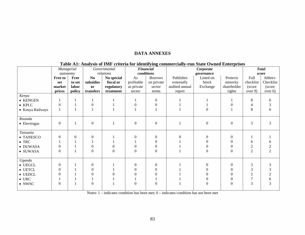
DATA ANNEXES

Table A1: Analysis of IMF criteria for identifying commercially-run State Owned Enterprises Managerial

autonomy Governmental

relations Financial conditions

Corporate governance

Total score

Free to set

market prices

Free to set labor policy

No subsidies

or transfers

No special fiscal or

regulatory treatment

As profitable as private

sector

Borrows on private

sector terms

Publishes externally

audited annual report

Listed on Stock

Exchange

Protects minority

shareholder rights

Full checklist

(score over 9)

Abbrev. Checklist

(score over 6)

Kenya • KENGEN 1 1 1 1 1 0 1 1 1 8 6 • KPLC 0 1 0 1 0 0 1 1 0 4 3 • Kenya Railways 1 1 1 1 1 1 1 0 1 8 6 Rwanda • Electrogaz 0 1 0 1 0 0 1 0 0 3 3 Tanzania • TANESCO 0 0 0 1 0 0 0 0 0 1 1 • TRC 1 1 1 1 1 0 1 0 0 6 6 • DUWASA 0 1 0 0 0 0 1 0 0 2 2 • SUWASA 0 1 0 0 0 0 1 0 0 2 2 Uganda • UEGCL 0 1 0 1 0 0 1 0 0 3 3 • UETCL 0 1 0 1 0 0 1 0 0 3 3 • UEDCL 0 1 0 0 0 0 1 0 0 2 2 • URC 1 1 1 1 1 1 1 0 0 7 6 • NWSC 0 1 0 1 0 0 1 0 0 3 3

Notes: 1 – indicates condition has been met; 0 – indicates condition has not been met

83

Table A2.1: Kenya – Detailed fiscal cost data (% GDP) Year Budget

type Sector Institution Expenditure

category 2000 2001 2002 2003 2004 2005 Average Wages and salaries 0.0029 0.0033 0.0048 0.0041 0.0037 Other current 0.7852 0.0062 0.0065 0.0056 0.2009 Capital 0.0035 0.4375 0.1283 0.2054 0.1937

Electricity

Central Gov’t Total 0.7916 0.4470 0.1396 0.2150 0.3983

Wages and salaries 0.0000 0.0000 0.0000 Other current 0.0400 0.0500 0.0450 Capital 0.0000 0.0000 0.0000

Railway

Central Gov’t Total 0.0424 0.0515 0.0469

Wages and salaries 0.0008 0.0945 0.0935 0.0804 0.0673 Other current 0.0065 0.0070 0.0046 0.0078 0.0065 Capital 0.1886 0.0992 0.2243 0.2492 0.1903

Central Gov’t Total 0.1959 0.2007 0.3225 0.3374 0.2641

Wages and salaries 0.0026 0.0069 0.0055 0.0065 0.0054 Other current 0.7670 0.7469 0.7993 0.7978 0.7778 Capital 0.0000 0.0000 0.0000 0.0000 0.0000

Road

KRB Total 0.7697 0.7538 0.8049 0.8043 0.7832

Wages and salaries 0.0000 0.0873 0.0437 Other current 0.0031 0.0669 0.0350 Capital 0.1421 0.2720 0.2071

Budget

Water

Central Gov’t Total 0.1453 0.4262 0.2857

Wages and salaries 0.1109 0.1163 0.1118 0.1101 0.1123 Other current 0.1567 0.1317 0.1081 0.1299 0.1316 Capital 0.5789 0.4713 0.2862 0.2983 0.4087

KENGEN Total 0.8465 0.7193 0.5061 0.5383 0.6526

Wages and salaries 0.4005 0.4287 0.3337 0.3275 0.3726 Other current 2.5141 2.2635 1.6816 1.8056 2.0662 Capital 0.1910 0.1186 0.2725 0.1450 0.1818

Electricity

KPLC Total 3.1057 2.8107 2.2878 2.2781 2.6206

Wages and salaries 0.1404 0.1354 0.1237 0.1043 0.1259 Other current 0.4167 0.3732 0.3143 0.2658 0.3425 Capital 0.0000 0.0000 0.0000 0.0000 0.0000

Non- Budget

Railway

Kenya Rail Total 0.5571 0.5086 0.4380 0.3701 0.4684

84

Table A2.2: Rwanda – Detailed fiscal cost data (% GDP) Year Budget

type Sector Institution Expenditure category

2000 2001 2002 2003 2004 2005 Average Wages and salaries 0.0000 0.0018 0.0020 0.0016 0.0010 0.0013 Other current 0.0000 0.0009 0.0006 0.0073 0.0022 Capital 0.0000 0.1005 0.2715 0.3513 1.1204 0.3687

Electricity

Central Gov’t Total 0.0000 0.1023 0.2743 0.3535 1.1287 0.3718

Wages and salaries 0.0000 0.0000 0.0000 0.0000 0.0000 0.0000 Other current 0.0000 0.0000 0.0000 0.0000 0.0000 0.0000 Capital 0.0000 0.0000 0.0000 0.0000 0.0034 0.0007

Railway

Central Gov’t Total 0.0000 0.0000 0.0000 0.0000 0.0034 0.0007

Wages and salaries 0.0000 0.0030 0.0151 0.0026 0.0016 0.0045 Other current 0.0296 0.0144 0.0328 0.0464 0.0308 Capital 0.0000 0.9587 0.2982 1.1511 1.1853 0.7187

Road

Central Gov’t Total 0.0000 0.9913 0.3277 1.1865 1.2332 0.7477

Wages and salaries 0.0000 0.0000 0.0043 0.0036 0.0026 0.0021 Other current 0.0016 0.0072 0.0091 0.0498 0.0169 Capital 0.0000 0.7235 0.4727 0.4901 0.6442 0.4661

Budget

Water

Central Gov’t Total 0.0000 0.7252 0.4842 0.5027 0.6967 0.4818

Wages and salaries 0.0000 0.1966 0.1781 0.1883 0.2143 0.1555 Other current 0.6560 0.6848 1.0658 1.2855 0.9230 Capital 0.0000 0.2394 0.1670 1.1868 0.1846 0.3556

Electricity

Electrogaz* Total 0.0000 1.0920 1.0300 2.4409 1.6845 1.2495

Wages and salaries 0.0000 0.0037 0.0043 0.0037 0.0040 0.0032 Other current 0.2011 0.3610 0.2558 0.2186 0.4157 0.2905 Capital 0.0000 0.0000 0.0000 0.0000 0.0000 0.0000

Road

FER Total 0.2011 0.3610 0.2558 0.2186 0.4157 0.2905

Wages and salaries 0.0000 0.0655 0.0594 0.0628 0.0071 0.0390 Other current 0.2187 0.2283 0.2023 0.2933 0.2356 Capital 0.0000 0.0822 0.0557 0.3956 0.0615 0.1190

Non- Budget

Water

Electrogaz* Total 0.0000 0.3664 0.3433 0.6607 0.3620 0.3465

85

Table A2.3: Tanzania – Detailed fiscal cost data (% GDP) Year Budget

type Sector Institution Expenditure category

2000 2001 2002 2003 2004 2005 Average Wages and salaries 0.0024 0.0031 0.0018 0.0020 0.1777 0.0374 Other current 0.0031 0.0559 0.1463 0.0394 0.8568 0.2203 Capital 0.3644 0.0000 0.0103 0.3534 0.0009 0.1458

Electricity

Central Gov’t Total 0.3700 0.0590 0.1584 0.3948 1.0354 0.4035

Wages and salaries 0.0000 0.0000 0.0000 0.0000 0.0000 0.0000 Other current 0.0000 0.0000 0.0000 0.0000 0.0000 0.0000 Capital 0.0000 0.0000 0.0093 0.0115 0.0000 0.0041

Railway

Central Gov’t Total 0.0000 0.0000 0.0093 0.0115 0.0000 0.0041

Wages and salaries 0.0194 0.0211 0.0092 0.0127 0.0000 0.0125 Other current 0.0086 0.5075 0.7224 0.7070 0.0000 0.3891 Capital 1.0735 0.0102 0.6037 0.6904 0.5945

Central Gov’t Total 1.1016 0.5388 1.3352 1.4102 0.0000 0.8772

Wages and salaries 0.0000 0.0216 0.0426 0.0152 0.0199 Other current 0.0061 0.0061 0.0280 0.0134 Capital 0.0000 0.0282 0.0265 0.0938 0.0371

Road

Local Gov’t Total 0.0000 0.0558 0.0753 0.1370 0.0670

Wages and salaries 0.0320 0.0312 0.0294 0.0260 0.0324 0.0302 Other current 0.0000 0.0308 0.0623 0.0317 0.0445 0.0339 Capital 0.0141 0.0030 0.0153 0.2868 0.7370 0.2113

Central Gov’t Total 0.0461 0.0650 0.1071 0.3445 0.8140 0.2754

Wages and salaries 0.0000 0.0043 0.0034 0.0125 0.0051 Other current 0.0162 0.0179 0.0366 0.0236 Capital 0.0000 0.0133 0.0287 0.0462 0.0220

Budget

Water

Local Gov’t Total 0.0000 0.0338 0.0500 0.0953 0.0448

86

Year Budget

type Sector Institution Expenditure category

2000 2001 2002 2003 2004 2005 Average Wages and salaries 0.1436 0.1054 0.0970 0.1364 0.1206 Other current 2.0826 1.7170 2.3693 2.3683 2.1343 Capital 1.5600 0.8000 0.7600 0.8200 0.9850

Electricity

TANESCO Total 3.7862 2.6224 3.2264 3.3247 3.2399

Wages and salaries 0.0006 0.0018 0.0035 0.0034 0.0023 Other current 0.6042 0.5677 0.5673 0.5503 0.5724 Capital 0.0000 0.0000 0.0000 0.0000 0.0000

Railway

TRC Total 0.6042 0.5677 0.5673 0.5503 0.5724

Wages and salaries 0.0000 0.0000 0.0460 0.0499 0.0240 Other current 0.5636 0.6453 0.5255 0.4703 0.5512 Capital 0.0000 0.0000 0.0000 0.0000 0.0000

Road

RFB Total 0.5636 0.6453 0.5715 0.5202 0.5752

Wages and salaries 0.0038 0.0032 0.0018 Other current 0.0137 0.0207 0.0172 Capital 0.0000 0.0000 0.0000

DUWASA Total 0.0137 0.0207 0.0086

Wages and salaries 0.0000 0.0000 0.0000 Other current 0.0800 0.0000 0.0400 Capital 0.0000 0.0000 0.0000

Non- Budget

Water

SUWASU Total 0.0800 0.0023 0.0412

87

Table A2.4: Uganda – Detailed fiscal cost data (% GDP) Year Budget

type Sector Institution Expenditure category

2000 2001 2002 2003 2004 2005 Average Wages and salaries 0.0102 0.0089 0.0095 Other current 0.1073 0.0788 0.0930 Capital 0.3339 0.3845 0.3592

Electricity

Central Gov’t Total 0.4514 0.4721 0.4618

Wages and salaries 0.0000 0.0000 0.0000 Other cu rrent Capital 0.0303 0.0679 0.0491

Railway

Central Gov’t Total 0.0303 0.0679 0.0491

Wages and salaries 0.0155 0.0262 0.0208 Other current 0.4918 0.4600 0.4759 Capital 1.4005 2.2794 1.8400

Road

Central Gov’t Total 1.9078 2.7657 2.3368

Wages and salaries 0.0229 0.0232 0.0230 Other current 0.1995 0.1521 0.1758 Capital 0.6519 0.6023 0.6271

Budget

Water

Central Gov’t Total 0.8743 0.7775 0.8259

88

Year Budget

type Sector Institution Expenditure category

2000 2001 2002 2003 2004 2005 Average Wages and salaries 0.0046 0.0072 0.0000 0.0000 0.0030 Other current 0.5435 0.0716 0.0000 0.0000 0.1538 Capital 0.0598 0.0022 0.0310

UEB Total 0.6080 0.0810 0.0000 0.0000 0.1723

Wages and salaries 0.0000 0.1199 0.1795 0.2079 0.1268 Other current 1.1076 0.7730 1.1275 1.0027 Capital 0.0000 0.0157 0.1057 0.1164 0.0594

UEDCL Total 0.0000 1.2432 1.0582 1.4518 0.9383

Wages and salaries 0.0182 0.0312 0.0100 0.0060 0.0163 Other current 0.1674 0.2301 0.1818 0.1619 0.1853 Capital 6.2830 0.3216 0.0617 0.3064 1.7432

UEGCL Total 6.4686 0.5829 0.2535 0.4743 1.9448

Wages and salaries 0.0167 0.0674 0.0390 0.0412 0.0411 Other current 0.4101 0.5373 0.3524 0.2515 0.3878 Capital 0.8836 0.0258 0.0175 0.0082 0.2338

Electricity

UETCL Total 1.3105 0.6305 0.4089 0.3010 0.6627

Wages and salaries 0.0944 0.0983 0.0856 0.0000 0.0696 Other current 0.3275 0.3017 0.2628 0.0000 0.2230 Capital 0.0124 0.0083 0.0000 0.0069

Railway

URC Total 0.4343 0.4083 0.3484 0.0000 0.2978

Wages and salaries 0.0000 0.0777 0.0849 0.1119 0.0686 Other current 0.2053 0.1833 0.1937 0.1941 Capital 0.0000 0.0379 0.0527 0.0596 0.0376

Non -Budget

Water

NWSC Total 0.0000 0.3209 0.3209 0.3651 0.2517

89