The BRAVO Effect in Queues(and more stuff about variance of output counts)

Yoni NazarathyThe University of Queensland

Presented in the Statistical Laboratory,Cambridge, May 20, 2014

1

Variance Collaborators

Daryl Daley Johan van Leeuwaarden

Ahmad Al-Hanbali Michel Mandjes Ward Whitt

Sophie Hautphenne Yoav Kerner Peter Taylor

Werner Scheinhardt Brendan Patch Thomas Taimre Gideon Weiss

2

Queueing Models

M/M/1, M/M/1/K , M/M/s/K , M/M/s/K+M ,

GI/G/1, GI/G/1/K , . . .

Basic conservation equation for a single queue

Q(t) = Q(0) +(A(t)− L(t)

)−(R(t) + D(t)

)

3

The Output Process D(·)

D(t) = Q(0) +(A(t)− L(t)− R(t)

)− Q(t)

Why analyse {D(t), t ≥ 0}?Orders

Production

Arrival process to a downstream queueing system

Some performance measures of interest

The law of {D(t), t ≥ 0}

E[D(t)], Var(D(t)

)λ∗ := limt→∞

E[D(t)]t , V := limt→∞

Var(

D(t))

t , D := Vλ∗

Asymptotic normality: D(t) ∼ N(λ∗t, V t

), large t

Second order approximations, e.g.,

Var(D(t)

)= V t + b + o(1)

Asymptotic covariances, etc...

4

The Output Process D(·)

D(t) = Q(0) +(A(t)− L(t)− R(t)

)− Q(t)

Why analyse {D(t), t ≥ 0}?Orders

Production

Arrival process to a downstream queueing system

Some performance measures of interest

The law of {D(t), t ≥ 0}

E[D(t)], Var(D(t)

)λ∗ := limt→∞

E[D(t)]t , V := limt→∞

Var(

D(t))

t , D := Vλ∗

Asymptotic normality: D(t) ∼ N(λ∗t, V t

), large t

Second order approximations, e.g.,

Var(D(t)

)= V t + b + o(1)

Asymptotic covariances, etc...

4

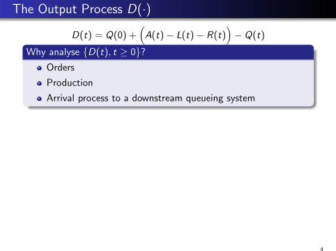
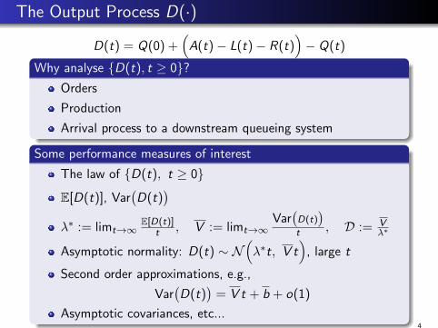
The Output Process D(·)

D(t) = Q(0) +(A(t)− L(t)− R(t)

)− Q(t)

Why analyse {D(t), t ≥ 0}?Orders

Production

Arrival process to a downstream queueing system

Some performance measures of interest

The law of {D(t), t ≥ 0}

E[D(t)], Var(D(t)

)λ∗ := limt→∞

E[D(t)]t , V := limt→∞

Var(

D(t))

t , D := Vλ∗

Asymptotic normality: D(t) ∼ N(λ∗t, V t

), large t

Second order approximations, e.g.,

Var(D(t)

)= V t + b + o(1)

Asymptotic covariances, etc...

4

The Output Process D(·)

D(t) = Q(0) +(A(t)− L(t)− R(t)

)− Q(t)

Why analyse {D(t), t ≥ 0}?Orders

Production

Arrival process to a downstream queueing system

Some performance measures of interest

The law of {D(t), t ≥ 0}

E[D(t)], Var(D(t)

)λ∗ := limt→∞

E[D(t)]t , V := limt→∞

Var(

D(t))

t , D := Vλ∗

Asymptotic normality: D(t) ∼ N(λ∗t, V t

), large t

Second order approximations, e.g.,

Var(D(t)

)= V t + b + o(1)

Asymptotic covariances, etc...4

Our Focus: Asymptotic Variance

Reminder: Poisson processes:

E[D(t)] = Var(D(t)

)= λt

Reminder: Renewal processes:

E[D(t)] ∼ λt Var(D(t)

)∼ λc2t

What is D = limt→∞Var(

D(t))

E[D(t)] for queues?

E.g. in stationary (and thus stable M/M/1): D = 1

5

Our Focus: Asymptotic Variance

Reminder: Poisson processes:

E[D(t)] = Var(D(t)

)= λt

Reminder: Renewal processes:

E[D(t)] ∼ λt Var(D(t)

)∼ λc2t

What is D = limt→∞Var(

D(t))

E[D(t)] for queues?

E.g. in stationary (and thus stable M/M/1): D = 1

5

Our Focus: Asymptotic Variance

Reminder: Poisson processes:

E[D(t)] = Var(D(t)

)= λt

Reminder: Renewal processes:

E[D(t)] ∼ λt Var(D(t)

)∼ λc2t

What is D = limt→∞Var(

D(t))

E[D(t)] for queues?

E.g. in stationary (and thus stable M/M/1): D = 1

5

Our Focus: Asymptotic Variance

Reminder: Poisson processes:

E[D(t)] = Var(D(t)

)= λt

Reminder: Renewal processes:

E[D(t)] ∼ λt Var(D(t)

)∼ λc2t

What is D = limt→∞Var(

D(t))

E[D(t)] for queues?

E.g. in stationary (and thus stable M/M/1): D = 1

5

Our Focus: Asymptotic Variance

Reminder: Poisson processes:

E[D(t)] = Var(D(t)

)= λt

Reminder: Renewal processes:

E[D(t)] ∼ λt Var(D(t)

)∼ λc2t

What is D = limt→∞Var(

D(t))

E[D(t)] for queues?

E.g. in stationary (and thus stable M/M/1): D = 1

5

For illustration, consider M/M/1/K

Let K be not so small, e.g. K = 40

Consider now λ� µ, e.g. λ = 0.5, µ = 1. What is D?

Consider now λ� µ e.g. λ = 2.0, µ = 1. What is D?

So how about D when λ = µ (e.g. = 1)?

Out[107]=

0.0 0.5 1.0 1.5 2.0Λ

2�3

1

Λ*,V D

0.0 0.5 1.0 1.5 2.0Λ

2�3

1

D = V D�Λ*

We call this BRAVO:

Balancing Reduces Asymptotic Variance of Outputs

6

For illustration, consider M/M/1/K

Let K be not so small, e.g. K = 40

Consider now λ� µ, e.g. λ = 0.5, µ = 1. What is D?

Consider now λ� µ e.g. λ = 2.0, µ = 1. What is D?

So how about D when λ = µ (e.g. = 1)?

Out[107]=

0.0 0.5 1.0 1.5 2.0Λ

2�3

1

Λ*,V D

0.0 0.5 1.0 1.5 2.0Λ

2�3

1

D = V D�Λ*

We call this BRAVO:

Balancing Reduces Asymptotic Variance of Outputs

6

For illustration, consider M/M/1/K

Let K be not so small, e.g. K = 40

Consider now λ� µ, e.g. λ = 0.5, µ = 1. What is D?

Consider now λ� µ e.g. λ = 2.0, µ = 1. What is D?

So how about D when λ = µ (e.g. = 1)?

Out[107]=

0.0 0.5 1.0 1.5 2.0Λ

2�3

1

Λ*,V D

0.0 0.5 1.0 1.5 2.0Λ

2�3

1

D = V D�Λ*

We call this BRAVO:

Balancing Reduces Asymptotic Variance of Outputs

6

For illustration, consider M/M/1/K

Let K be not so small, e.g. K = 40

Consider now λ� µ, e.g. λ = 0.5, µ = 1. What is D?

Consider now λ� µ e.g. λ = 2.0, µ = 1. What is D?

So how about D when λ = µ (e.g. = 1)?

Out[107]=

0.0 0.5 1.0 1.5 2.0Λ

2�3

1

Λ*,V D

0.0 0.5 1.0 1.5 2.0Λ

2�3

1

D = V D�Λ*

We call this BRAVO:

Balancing Reduces Asymptotic Variance of Outputs

6

For illustration, consider M/M/1/K

Let K be not so small, e.g. K = 40

Consider now λ� µ, e.g. λ = 0.5, µ = 1. What is D?

Consider now λ� µ e.g. λ = 2.0, µ = 1. What is D?

So how about D when λ = µ (e.g. = 1)?

Out[107]=

0.0 0.5 1.0 1.5 2.0Λ

2�3

1

Λ*,V D

0.0 0.5 1.0 1.5 2.0Λ

2�3

1

D = V D�Λ*

We call this BRAVO:

Balancing Reduces Asymptotic Variance of Outputs

6

For illustration, consider M/M/1/K

Let K be not so small, e.g. K = 40

Consider now λ� µ, e.g. λ = 0.5, µ = 1. What is D?

Consider now λ� µ e.g. λ = 2.0, µ = 1. What is D?

So how about D when λ = µ (e.g. = 1)?

Out[107]=

0.0 0.5 1.0 1.5 2.0Λ

2�3

1

Λ*,V D

0.0 0.5 1.0 1.5 2.0Λ

2�3

1

D = V D�Λ*

We call this BRAVO:

Balancing Reduces Asymptotic Variance of Outputs6

Finite Birth-Death Asymptotic Variance (and BRAVO)

7

Finite Birth-Death Setting

Irreducible birth-death process on finite state space

Birth rates: λ0, . . . , λJ−1

Death rates: µ1, . . . , µJ

Stationary distribution: π0, . . . , πJ

D(t) is number of downward transitions (deaths) during [0, t],each “filtered” independently with state-dependentprobabilities, q1, . . . , qJ .

e.g. The output process (served customers) in M/M/s/K+M :

λi = λ, µi = µ (i∧s)+γ (i−s)+, qi =µ (i ∧ s)

µ (i ∧ s) + γ (i − s)+, i = 0, 1, . . . , s+K

Of interest:

D =V

λ∗= lim

t→∞

Var(D(t)

)E[D(t)]

8

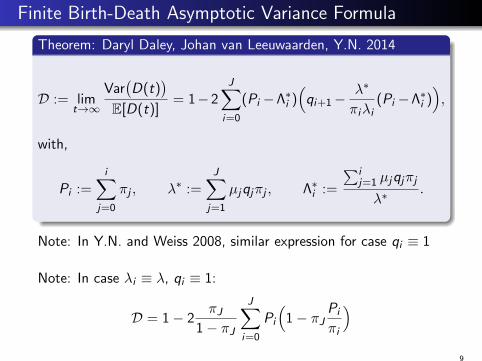
Finite Birth-Death Asymptotic Variance Formula

Theorem: Daryl Daley, Johan van Leeuwaarden, Y.N. 2014

D := limt→∞

Var(D(t)

)E[D(t)]

= 1−2J∑

i=0

(Pi −Λ∗i )(qi+1−

λ∗

πiλi(Pi −Λ∗i )

),

with,

Pi :=i∑

j=0

πj , λ∗ :=J∑

j=1

µjqjπj , Λ∗i :=

∑ij=1 µjqjπj

λ∗.

Note: In Y.N. and Weiss 2008, similar expression for case qi ≡ 1

Note: In case λi ≡ λ, qi ≡ 1:

D = 1− 2πJ

1− πJ

J∑i=0

Pi

(1− πJ

Pi

πi

)9

Idea of Renewal Reward Derivation

”Embed” D(t) in a Renewal-Reward Process, C (t)

1 (Xn,Yn) ≡ (busy cycle, number served) in cycle n

2 N(t) = sup{n :∑n

i=1 Xi ≤ t}, C (t) =∑N(t)

i=1 Yi

3 Asymptotic variance rates of C (t) and D(t) are equal

4 Known:– Asymptotic variance rate of C (t) is 1

E[X ] Var(Y − E[Y ]

E[X ]X)

– Systems of equations for1’st, 2’nd and cross moments of X and Y

X1

X2

X3

Y1

Y2

Y3

DHtLCHtL

t

10

Back to the M/M/1/K Queue

Here πi is truncated geometric distribution when λ 6= µ and auniform distribution when λ = µ

Using D = 1− 2 πJ1−πJ

∑Ji=0 Pi

(1− πJ

Piπi

):

D =

{1 + oK (1), λ 6= µ,23 + oK (1), λ = µ.

0.0 0.5 1.0 1.5 2.0Λ

2�3

1

Λ*, V

M�M�1�K=10

0.0 0.5 1.0 1.5 2.0Λ

2�3

1

Λ*, V

M�M�1�K=40

0.0 0.5 1.0 1.5 2.0Λ

2�3

1

Λ*, V

M�M�1�K=100

In fact, for any λ, µ, we have an explicit expression for D (alt. V , λ∗)and even for b in,

Var(D(t)

)= V t + b + o(1)

11

Back to the M/M/1/K Queue

Here πi is truncated geometric distribution when λ 6= µ and auniform distribution when λ = µ

Using D = 1− 2 πJ1−πJ

∑Ji=0 Pi

(1− πJ

Piπi

):

D =

{1 + oK (1), λ 6= µ,23 + oK (1), λ = µ.

0.0 0.5 1.0 1.5 2.0Λ

2�3

1

Λ*, V

M�M�1�K=10

0.0 0.5 1.0 1.5 2.0Λ

2�3

1

Λ*, V

M�M�1�K=40

0.0 0.5 1.0 1.5 2.0Λ

2�3

1

Λ*, V

M�M�1�K=100

In fact, for any λ, µ, we have an explicit expression for D (alt. V , λ∗)and even for b in,

Var(D(t)

)= V t + b + o(1)

11

Back to the M/M/1/K Queue

Here πi is truncated geometric distribution when λ 6= µ and auniform distribution when λ = µ

Using D = 1− 2 πJ1−πJ

∑Ji=0 Pi

(1− πJ

Piπi

):

D =

{1 + oK (1), λ 6= µ,23 + oK (1), λ = µ.

0.0 0.5 1.0 1.5 2.0Λ

2�3

1

Λ*, V

M�M�1�K=10

0.0 0.5 1.0 1.5 2.0Λ

2�3

1

Λ*, V

M�M�1�K=40

0.0 0.5 1.0 1.5 2.0Λ

2�3

1

Λ*, V

M�M�1�K=100

In fact, for any λ, µ, we have an explicit expression for D (alt. V , λ∗)and even for b in,

Var(D(t)

)= V t + b + o(1)

11

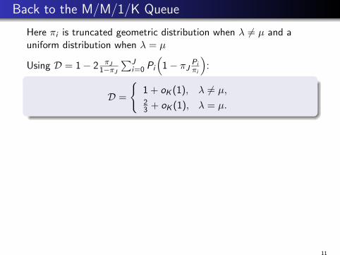
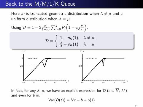
Back to the M/M/1/K Queue

Here πi is truncated geometric distribution when λ 6= µ and auniform distribution when λ = µ

Using D = 1− 2 πJ1−πJ

∑Ji=0 Pi

(1− πJ

Piπi

):

D =

{1 + oK (1), λ 6= µ,23 + oK (1), λ = µ.

0.0 0.5 1.0 1.5 2.0Λ

2�3

1

Λ*, V

M�M�1�K=10

0.0 0.5 1.0 1.5 2.0Λ

2�3

1

Λ*, V

M�M�1�K=40

0.0 0.5 1.0 1.5 2.0Λ

2�3

1

Λ*, V

M�M�1�K=100

In fact, for any λ, µ, we have an explicit expression for D (alt. V , λ∗)and even for b in,

Var(D(t)

)= V t + b + o(1)

11

Multi-Server Systems in the Halfin-Whitt (QED) Regime

12

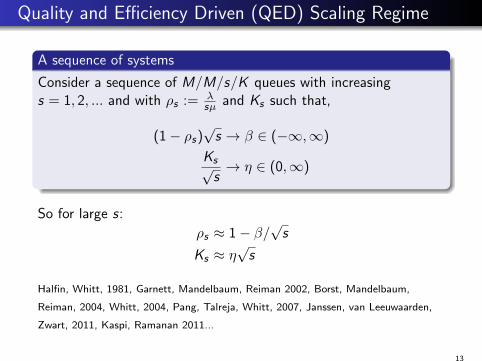
Quality and Efficiency Driven (QED) Scaling Regime

A sequence of systems

Consider a sequence of M/M/s/K queues with increasings = 1, 2, ... and with ρs := λ

sµ and Ks such that,

(1− ρs)√s → β ∈ (−∞,∞)

Ks√s→ η ∈ (0,∞)

So for large s:

ρs ≈ 1− β/√s

Ks ≈ η√s

Halfin, Whitt, 1981, Garnett, Mandelbaum, Reiman 2002, Borst, Mandelbaum,

Reiman, 2004, Whitt, 2004, Pang, Talreja, Whitt, 2007, Janssen, van Leeuwaarden,

Zwart, 2011, Kaspi, Ramanan 2011...

13

Favorable QED Properties

Probability of delay converges to a value ∈ (0, 1)

Mean waiting times are typically O(s−1/2)

Large queue lengths almost never occur

Quick mixing times

In applications: Call-centers (etc...) describes behavior welland allows for asymptotic approximate optimization of staffingetc...

How about BRAVO?

14

M/M/s/b√sc

0.6 0.8 1.0 1.2 1.4 r

0.2

0.4

0.6

0.8

1.0Dp

s=9

s=100

s=900s=104

D0,1

15

M/M/s/K QED BRAVO

Theorem: Daryl Daley, Johan van Leeuwaarden, Y.N. 2013

Consider QED scaling with β 6= 0:

Dβ,η := lims,K→∞

limt→∞

Var(D(t)

)E(D(t)

) ,Dβ,η = 1− 2β2e−βηh2

φ(β)

∫ ∞−β

(1− βe−βηhΦ(−u)

φ(u)

)Φ(−u) du

+ 2e−βηh(1 + e−βηh)(

1− βη − e−βη + (1− 2βηe−βη − e−2βη)h)

where

h = lims→∞

P(Qs ≥ s)

1− e−βη=

1

1− e−βη + βΦ(β)φ(β)

16

BRAVO Viewed Through the QED Lens

-4 -2 0 2 4Β

0.6

0.7

0.8

0.9

1.0

DΒ,Η

Η=0.232

Η=1

Η=2

17

0.6 0.8 1.0 1.2 1.4 r

0.2

0.4

0.6

0.8

1.0Dp

s=9

s=100

s=900s=104

D0,1

18

M/M/s/K QED BRAVO with ρ ≡ 1 (β = 0)

Theorem: Daryl Daley, Johan van Leeuwaarden, Y.N. 2013

Assume ρ ≡ 1 and Ks√s→ η ∈ (0,∞). Then

D0,η := lims,K→∞

limt→∞

Var(D(t)

)E(D(t)

) ,D0,η =

2

3−(6− 3π

2

)η − 1

2π√

π2 + 3

√2π(1− log 2)

3(η +

√π2

)3.

19

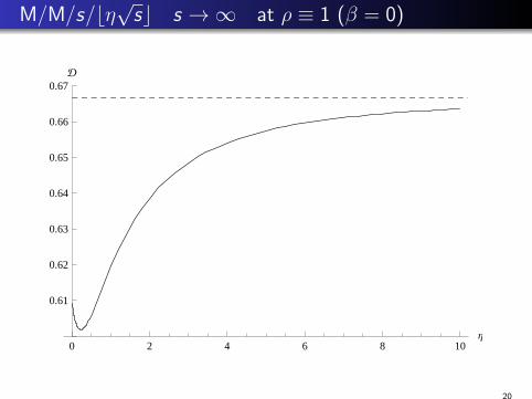
M/M/s/bη√sc s →∞ at ρ ≡ 1 (β = 0)

0 2 4 6 8 10Η

0.61

0.62

0.63

0.64

0.65

0.66

0.67D

20

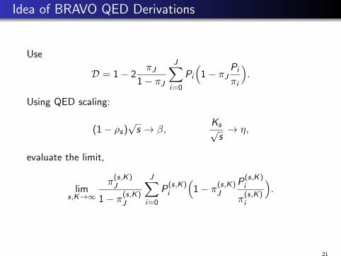
Idea of BRAVO QED Derivations

Use

D = 1− 2πJ

1− πJ

J∑i=0

Pi

(1− πJ

Pi

πi

).

Using QED scaling:

(1− ρs)√s → β,

Ks√s→ η,

evaluate the limit,

lims,K→∞

π(s,K)J

1− π(s,K)J

J∑i=0

P(s,K)i

(1− π(s,K)

J

P(s,K)i

π(s,K)i

).

21

Beyond Finite Birth-Death Queues

22

M/M/1 Queue

When K =∞, the birth-death D formula, generally does not hold.In this case,

D =

{1, λ 6= µ,

?, λ = µ.

A guess is 23 , since for K <∞, D = 2

3 + oK (1) . . .

Theorem:Ahmad Al-Hanbali, Michel Mandjes, Y. N., Ward Whitt, 2011

For the M/M/1 queue with λ = µ and arbitrary initial conditionsof Q(0) (with finite second moments),

D = 2(

1− 2

π

)≈ 0.727.

Proof based on analysis of classic Laplace transform of thegenerating function of D(·)

23

M/M/1 Queue

When K =∞, the birth-death D formula, generally does not hold.In this case,

D =

{1, λ 6= µ,

?, λ = µ.

A guess is 23 , since for K <∞, D = 2

3 + oK (1) . . .

Theorem:Ahmad Al-Hanbali, Michel Mandjes, Y. N., Ward Whitt, 2011

For the M/M/1 queue with λ = µ and arbitrary initial conditionsof Q(0) (with finite second moments),

D = 2(

1− 2

π

)≈ 0.727.

Proof based on analysis of classic Laplace transform of thegenerating function of D(·)

23

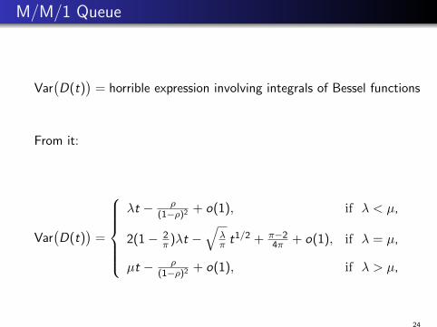
M/M/1 Queue

Var(D(t)

)= horrible expression involving integrals of Bessel functions

From it:

Var(D(t)

)=

λt − ρ

(1−ρ)2 + o(1), if λ < µ,

2(1− 2π )λt −

√λπ t

1/2 + π−24π + o(1), if λ = µ,

µt − ρ(1−ρ)2 + o(1), if λ > µ,

24

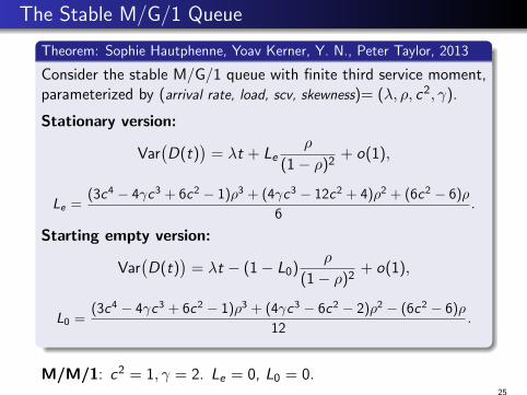
The Stable M/G/1 Queue

Theorem: Sophie Hautphenne, Yoav Kerner, Y. N., Peter Taylor, 2013

Consider the stable M/G/1 queue with finite third service moment,parameterized by (arrival rate, load, scv, skewness)= (λ, ρ, c2, γ).

Stationary version:

Var(D(t)

)= λt + Le

ρ

(1− ρ)2+ o(1),

Le =(3c4 − 4γc3 + 6c2 − 1)ρ3 + (4γc3 − 12c2 + 4)ρ2 + (6c2 − 6)ρ

6.

Starting empty version:

Var(D(t)

)= λt − (1− L0)

ρ

(1− ρ)2+ o(1),

L0 =(3c4 − 4γc3 + 6c2 − 1)ρ3 + (4γc3 − 6c2 − 2)ρ2 − (6c2 − 6)ρ

12.

M/M/1: c2 = 1, γ = 2. Le = 0, L0 = 0.25

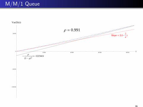
M/M/1 Queue

20 000 40 000 60 000 80 000t

-100 000

-50 000

0

50 000

VarHDHtLL

-Ρ

H1 - ΡL2=-12234.6

Slope = 2H1-2Π

LΡ = 0.991

26

M/M/1 Queue

20 000 40 000 60 000 80 000t

-100 000

-50 000

0

50 000

VarHDHtLL

-Ρ

H1 - ΡL2=-20265.3

Slope = 2H1-2Π

LΡ = 0.993

27

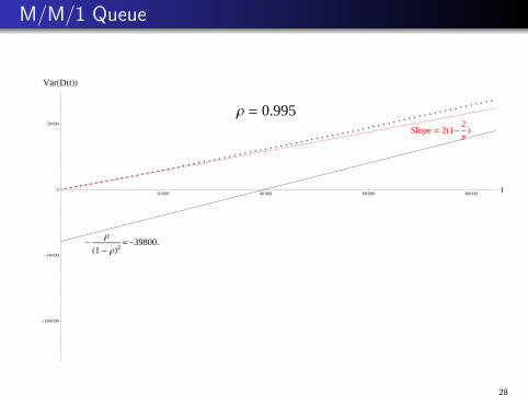
M/M/1 Queue

20 000 40 000 60 000 80 000t

-100 000

-50 000

0

50 000

VarHDHtLL

-Ρ

H1 - ΡL2=-39800.

Slope = 2H1-2Π

LΡ = 0.995

28

M/M/1 Queue

20 000 40 000 60 000 80 000t

-100 000

-50 000

0

50 000

VarHDHtLL

-Ρ

H1 - ΡL2=-110778.

Slope = 2H1-2Π

LΡ = 0.997

29

GI/G/1 Queue

Moving away from the memory-less assumptions,

D =

c2

a , λ < µ,

?, λ = µ,

c2s , λ > µ.

For M/M/1 it was 2(1− 2π )...

Theorem:Ahmad Al-Hanbali, Michel Mandjes, Y.N., Ward Whitt, 2011

For the GI/G/1 queue with λ = µ, arbitrary finite second momentinitial conditions

(Q(0),V (0),U(0)

), finite fourth moments of the

inter-arrival and service times, and P(B > x) ∼ L(x)x−1/2, whereB denotes the busy period and L(·) is a slowly varying function,

D = (c2a + c2

s )(

1− 2

π

).

Proof using diffusion limit of (D(n·)− λn·)/√λn· as n→∞ (Iglehart and Whitt 1971).

30

GI/G/1 Queue

Moving away from the memory-less assumptions,

D =

c2

a , λ < µ,

?, λ = µ,

c2s , λ > µ.

For M/M/1 it was 2(1− 2π )...

Theorem:Ahmad Al-Hanbali, Michel Mandjes, Y.N., Ward Whitt, 2011

For the GI/G/1 queue with λ = µ, arbitrary finite second momentinitial conditions

(Q(0),V (0),U(0)

), finite fourth moments of the

inter-arrival and service times, and P(B > x) ∼ L(x)x−1/2, whereB denotes the busy period and L(·) is a slowly varying function,

D = (c2a + c2

s )(

1− 2

π

).

Proof using diffusion limit of (D(n·)− λn·)/√λn· as n→∞ (Iglehart and Whitt 1971).

30

GI/G/1/K Queue

D =

c2

a + oK (1), λ < µ,

?, λ = µ,

c2s + oK (1), λ > µ.

For M/M/1/K it was 23 + oK (1), for GI/G/1 it was

(c2a + c2

s )(1− 2π )...

Conjecture (numerically tested): Y.N., 2011

For the GI/G/1/K queue with λ = µ and arbitrary initialconditions and light-tailed service and inter-arrival times,

D = (c2a + c2

s )1

3+ O

( 1

K

).

Numerical verification done by representing the system asPH/PH/1/K MAPs

31

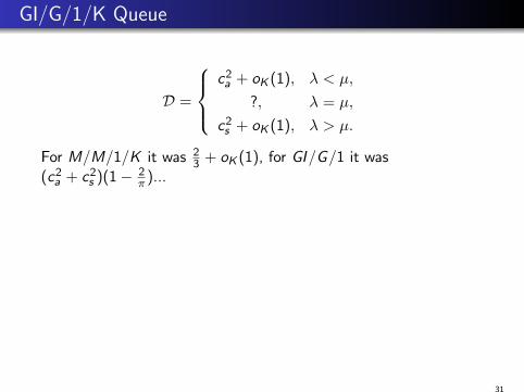
GI/G/1/K Queue

D =

c2

a + oK (1), λ < µ,

?, λ = µ,

c2s + oK (1), λ > µ.

For M/M/1/K it was 23 + oK (1), for GI/G/1 it was

(c2a + c2

s )(1− 2π )...

Conjecture (numerically tested): Y.N., 2011

For the GI/G/1/K queue with λ = µ and arbitrary initialconditions and light-tailed service and inter-arrival times,

D = (c2a + c2

s )1

3+ O

( 1

K

).

Numerical verification done by representing the system asPH/PH/1/K MAPs

31

Wrap Up

32

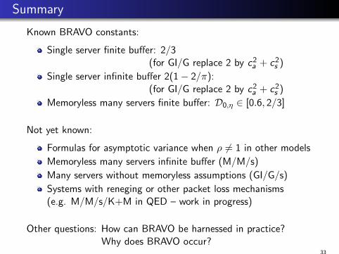
Summary

Known BRAVO constants:

Single server finite buffer: 2/3(for GI/G replace 2 by c2

a + c2s )

Single server infinite buffer 2(1− 2/π):(for GI/G replace 2 by c2

a + c2s )

Memoryless many servers finite buffer: D0,η ∈ [0.6, 2/3]

Not yet known:

Formulas for asymptotic variance when ρ 6= 1 in other models

Memoryless many servers infinite buffer (M/M/s)

Many servers without memoryless assumptions (GI/G/s)

Systems with reneging or other packet loss mechanisms(e.g. M/M/s/K+M in QED – work in progress)

Other questions: How can BRAVO be harnessed in practice?Why does BRAVO occur?

33

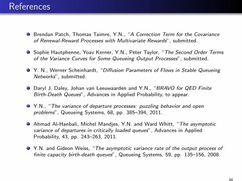
References

Brendan Patch, Thomas Taimre, Y.N., “A Correction Term for the Covarianceof Renewal-Reward Processes with Multivariate Rewards”, submitted.

Sophie Hautphenne, Yoav Kerner, Y.N., Peter Taylor, “The Second Order Termsof the Variance Curves for Some Queueing Output Processes”, submitted.

Y. N., Werner Scheinhardt, “Diffusion Parameters of Flows in Stable QueueingNetworks”, submitted.

Daryl J. Daley, Johan van Leeuwaarden and Y.N., “BRAVO for QED FiniteBirth-Death Queues”, Advances in Applied Probability, to appear.

Y.N., “The variance of departure processes: puzzling behavior and openproblems”, Queueing Systems, 68, pp. 385–394, 2011.

Ahmad Al-Hanbali, Michel Mandjes, Y.N. and Ward Whitt, “The asymptoticvariance of departures in critically loaded queues”, Advances in AppliedProbability, 43, pp. 243–263, 2011.

Y.N. and Gideon Weiss, “The asymptotic variance rate of the output process offinite capacity birth-death queues”, Queueing Systems, 59, pp. 135–156, 2008.

34