Week 5: The Hardy-Weinberg equilibrium, population ... · Lauren Phillips Introduction to Genetics...

Lauren Phillips Introduction to Genetics and Evolution, Winter 2014

Mohamed A.F. Noor, Duke University

Week 5: The Hardy-Weinberg equilibrium, population differences and inbreeding

5.1: Allele and genotype frequencies Two questions we’ll answer by looking at variation, one gene at a time:

Can we predict genotype frequencies from allele frequencies? If “sometimes,” when? Do genotype frequencies intrinsically change over time, or do they remain constant?

A hypothetical scenario:

Two alleles A and a and three possible genotypes AA, Aa and aa Each has a frequency, totaling 100%

Example: If 78% of alleles are A, 22% are a 25% of individuals are AA and 50% are Aa, so 25% are aa.

Calculating genotype frequencies: Assuming every individual is diploid (2N), we can get them by counting

(population info from a box shown in slide) Total number of individuals = 10 Frequency AA = 1/10 = 0.1 Frequency Aa = 6/10 = 0.6 Frequency aa = 3/10 = 0.3 The total ALWAYS adds up to 1.

Calculating allele frequencies Assuming every individual is diploid (also, this is same population as above) We could count the A’s and a’s:

20 total alleles (10 genotypes) freq(A) = 8/20 = 0.4 freq(a) = 12/20 = 0.6

But here’s a better way: freq(A) = freq_AA + ½ freq_Aa = 0.1 + ½(0.6)= 0.4 freq(a) = freq_aa + ½ freq_Aa = 0.3 + ½(0.6) = 0.6

One could think of the world as a pool of gametes (or not, because that’s kind of icky) All individuals of sexual species start as 2 gametes

Gametes are 1N Many marine invertebrates “spew” gametes into the water that make

individuals We can use joint probability multiplication to determine genotype frequencies in

offspring 60% of sperm are A and 60% of eggs are A

40% of sperm are a and 40% of eggs are a What’s the probability of an AA individual?



The joint probability that fertilization involves an A sperm and an A egg.

So, 0.6 x 0.6 = 36% The probability of aa is calculated the same way: 0.4 x 0.4 = 0.16 But there are TWO ways to make an Aa zygote.

A sperm + a egg → 0.6 x 0.4 = 0.24 a sperm + A egg → 0.4 x 0.6 = 0.24 add those together and you get 0.48

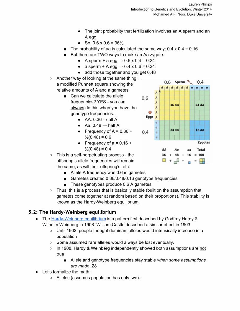
Another way of looking at the same thing: a modified Punnett square showing the relative amounts of A and a gametes

Can we calculate the allele frequencies? YES you can always do this when you have the genotype frequencies.

AA: 0.36 → all A Aa: 0.48 → half A Frequency of A = 0.36 +

½(0.48) = 0.6 Frequency of a = 0.16 +

½(0.48) = 0.4 This is a selfperpetuating process the

offspring’s allele frequencies will remain the same, as will their offspring’s, etc.

Allele A frequency was 0.6 in gametes Gametes created 0.36/0.48/0.16 genotype frequencies These genotypes produce 0.6 A gametes

Thus, this is a process that is basically stable (built on the assumption that gametes come together at random based on their proportions). This stability is known as the HardyWeinberg equilibrium.

5.2: The Hardy-Weinberg equilibrium The HardyWeinberg equilibrium is a pattern first described by Godfrey Hardy &

Wilhelm Weinberg in 1908. William Castle described a similar effect in 1903. Until 1902, people thought dominant alleles would intrinsically increase in a

population Some assumed rare alleles would always be lost eventually. In 1908, Hardy & Weinberg independently showed both assumptions are not

true Allele and genotype frequencies stay stable when some assumptions

are made..28 Let’s formalize the math:

Alleles (assumes population has only two):

http://en.wikipedia.org/wiki/Hardy%E2%80%93Weinberg_principle



Frequency of A = p Frequency of a = q p + q = 1

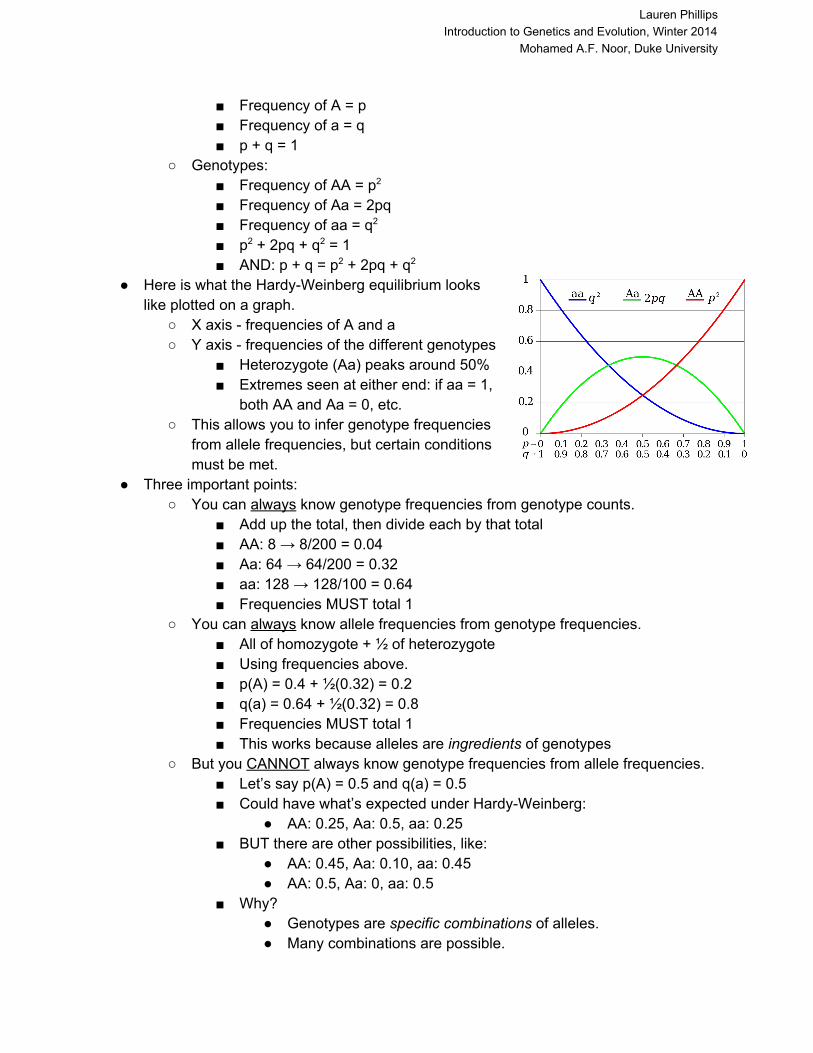
Genotypes: Frequency of AA = p2 Frequency of Aa = 2pq Frequency of aa = q2 p2 + 2pq + q2 = 1 AND: p + q = p2 + 2pq + q2

Here is what the HardyWeinberg equilibrium looks like plotted on a graph.

X axis frequencies of A and a Y axis frequencies of the different genotypes

Heterozygote (Aa) peaks around 50% Extremes seen at either end: if aa = 1,

both AA and Aa = 0, etc. This allows you to infer genotype frequencies

from allele frequencies, but certain conditions must be met.

Three important points: You can always know genotype frequencies from genotype counts.

Add up the total, then divide each by that total AA: 8 → 8/200 = 0.04 Aa: 64 → 64/200 = 0.32 aa: 128 → 128/100 = 0.64 Frequencies MUST total 1

You can always know allele frequencies from genotype frequencies. All of homozygote + ½ of heterozygote Using frequencies above. p(A) = 0.4 + ½(0.32) = 0.2 q(a) = 0.64 + ½(0.32) = 0.8 Frequencies MUST total 1 This works because alleles are ingredients of genotypes

But you CANNOT always know genotype frequencies from allele frequencies. Let’s say p(A) = 0.5 and q(a) = 0.5 Could have what’s expected under HardyWeinberg:

AA: 0.25, Aa: 0.5, aa: 0.25 BUT there are other possibilities, like:

AA: 0.45, Aa: 0.10, aa: 0.45 AA: 0.5, Aa: 0, aa: 0.5

Why? Genotypes are specific combinations of alleles. Many combinations are possible.



So, back to HardyWeinberg: It allows the prediction of genotype frequencies from allele frequencies under

certain conditions: Random mating (multiplying probabilities rule) No selection, migration or mutation at that locus Infinite population size no “genetic drift” In short, it predicts a completely boring population that probably could

never exist. So why bother? It provides a null hypothesis.

By seeing how natural populations deviate from the HW expected genotype frequencies, we infer what interesting evolutionary forces are operating.

Testing for HardyWeinberg Is this at HW? → AA: 245, Aa: 210, aa: 45

Figure out true genotype frequencies total = 500 AA: 245/500 = 0.49 Aa: 210/500 = 0.42 aa: 45/500 = 0.09

Figure out true allele frequencies p(A) = 0.49 + 0.21 = 0.7 q(a) = 0.09 + 0.21 = 0.3

Figure out HW “expected” genotype frequencies p + q = p2 + 2pq + q2 p2 = 0.72 = 0.49 2pq = 2(0.7)(0.3) = 0.42 q2 = 0.32 = 0.09

Do true frequencies = expected frequencies? YES!

One for you to try on your own: AA: 400, Aa: 200, aa: 400 Figure out true genotype frequencies

total = 1000 AA: 400/1000 = 0.4 Aa: 200/1000 = 0.2 aa: 400/1000 = 0.4

Figure out true allele frequencies p(A) = 0.4 + 0.1 = 0.5 q(a) = 0.4 + 0.2 = 0.5

Figure out HW “expected” genotype frequencies p + q = p2 + 2pq + q2 p2 = 0.25 2pq = 0.5 q2 = 0.25



Do true frequencies = expected frequencies? Not this time.

5.3: Deviation from Hardy-Weinberg equilibrium - the Wahlund effect Real data:

Navajo populations MN blood type:

MM: 305 → 0.845 p(M) = 0.917 MN: 52 → 0.144 q(N) = 0.083 NN: 4 → 0.011 Total: 361

HW predicted (very close): MM: 0.841 MN: 0.152 NN: 0.007

Aborigine populations MN blood type:


HW predicted (again, very close): MM: 0.031 MN: 0.293 NN: 0.676

Mixed population of both of the above MN blood type:


HW predicted (NOT close this time) MM: 0.179 MN: 0.488 NN: 0.333 Dramatically different from the two individual groups

predicts nearly half MN, when we actually get ¼ Why might we see this deviation the combination of two HW groups being nonHW?

We cannot assume random mating that any two individuals as likely to breed as any other two individuals

A Navajo lady isn’t as likely to breed with an Aborigine as she is with another Navajo.

The result is too few heterozygotes 0.246 observed, rather than expected 0.488



This is called the Wahlund effect: sampling across populations gives an underrepresentation of heterozygotes relative to HW.

Why does it matter if something is HW or not? The first step in genomewide association studies of genetic diseases is usually

to test for HW. Why? Because GWAS assumes HW (or nearly so)

Assumes linkage disequilibrium detected between marker alleles and disease alleles is caused by close proximity/lack of recombination.

20% of those with AA genotype have disease 5% of those with aa genotype have disease Thus, association between A marker genotype and disease

Being in different populations (ie, nonrandom mating) also creates LD. An extreme example:

Population 1 is all AA and Population 2 is all aa If disease is more abundant in P1 than P2 …

Would you say AA is more likely to have the disease than aa? Yes.

This is actually a fake LD between disease and gene A. The disease gene may be on a different chromosome, or

the disease may not even be influenced by genetics at all.

If there are allele frequency differences between populations at a SNP, and there are disease incidence differences between those populations, it’ll erroneously look like a gene near the SNP causes or contributes to the disease.

Testing for HW helps you avoid this error it identifies if you’re looking at one interbreeding population or more.

Although it’s very important to test for HW, it’s often not done … 2006 study: Exclusion of studies in which HW was violated changed

conclusions and statistical significance of genedisease associations 2005 study: testing/reporting for HW is often neglected; published

reports rarely admit the deviations. A real example where an HW test WAS done but misinterpreted:

2000 study of BRCA2 variants (newborn males from UK hospital) AA: 644 → 0.539 p(A) = 0.721 Aa: 435 → 0.364 q(a) = 0.279 aa: 116 → 0.097 Total: 1195

p2 = 0.520 2pq = 0.402 q2 = 0.078 A statistically significant deviation from HW too few Aa (heterozygotes)

observed.



The authors inferred that Aa are less healthy than AA or aa. A much more likely conclusion: A place like London has lots of subsets

of the population. People of Indian descent, for example, are more likely to have kids with others from their group.

An ironic tidbit to end on: At age 62, lamenting the waning of his math ability, Hardy wrote that he’d “never done anything ‘useful’” never made a discovery that made “the least difference in the amenity of the world.” He was very wrong on this.

5.4: Differences between populations - origins and quantifying Recap: Navajo and Aborigine populations each showed HW equilibrium in blood type

genotype frequencies, but the combination of the two populations did not there was a deficiency of heterozygotes from what would be expected under HW. This is what’s called the Wahlund effect.

Populations differ: May have different allele and genotype frequencies But they may also have alleles at some genes not found in other populations if

it’s a very recent new mutation, or populations are in complete isolation

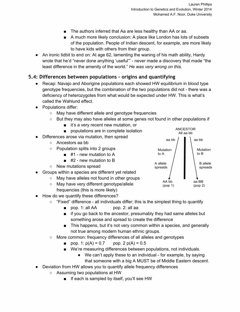
Differences arose via mutation, then spread Ancestors aa bb Population splits into 2 groups

#1 new mutation to A #2 new mutation to B

New mutations spread Groups within a species are different yet related

May have alleles not found in other groups May have very different genotype/allele

frequencies (this is more likely) How do we quantify these differences?

“Fixed” difference all individuals differ; this is the simplest thing to quantify pop. 1: all AA pop. 2: all aa if you go back to the ancestor, presumably they had same alleles but

something arose and spread to create the difference This happens, but it’s not very common within a species, and generally

not true among modern human ethnic groups. More common: frequency differences of all alleles and genotypes

pop. 1: p(A) = 0.7 pop. 2 p(A) = 0.5 We’re measuring differences between populations, not individuals.

We can’t apply these to an individual for example, by saying that someone with a big A MUST be of Middle Eastern descent.

Deviation from HW allows you to quantify allele frequency differences Assuming two populations at HW

If each is sampled by itself, you’ll see HW



If both are sampled together, you’ll see deviation from HW (Wahlund effect)

How large the deviation is from HW when both are sampled together quantifies the difference in allele frequencies.

The measure we’ll use is FST Ranges from 0 to 1

0: no allele frequency differences 0 < FST < 1: allele frequencies differ somewhat 1: “fixed” difference between populations

FST = HW predicted 2pq % observed heterozygotes HW predicted 2pq

Example: Pop. 1: Pop. 2

AA: 100 AA: 0 Aa: 0 Aa: 0 aa: 0 aa: 100

Total: AA: 100, Aa: 0, aa: 100 (total genotype count = 200) AA = .37+.24 = 0.5 p(A) and q(a) = 0.5

Aa = 0 HW 2pq = 0.5 (observed = 0) aa = 0.5

FST = (0.50)/0.5 = 1 fixed difference Another, less extreme, example:

Pop. 1: Pop. 2 AA: 250 AA: 490 Aa: 500 Aa: 420 aa: 250 aa: 90

Total: AA: 740, Aa: 920, aa: 340 (total genotype count = 2000) AA = 740/2000 = 0.37 p(A) = 0.6

Aa = 920/2000 = 0.46 q(a) = 0.4 aa = 340/2000 = 0.17 HW 2pq = 0.48 (observed = 0.46)

FST = (0.48 0.46)/0.48 = 0.042 Now try using the real data from the NavajoAborigine mix:

MN blood type totals: MM: 327 MN: 268 NN: 496 Total: 1091

Observed: MM: 0.30 p(M) = 0.423 MN = 0.246 q(N) = 0.577 NN = 0.454 HW 2MN = 0.488

FST = (0.4880.246)/0.488 = 0.496 a fairly large FST consistent with the idea of no gene flow between the two populations.



Recap: FST is larger when comparing populations that are more different in allele

frequencies. If allele frequencies are identical, FST = 0. If a fixed difference, FST = 1

FST measures among human populations (data from 1,110,338 SNPs in a 2010 study) AfricanAmericans/Europeans: FST = 0.11 AfricanAmericans/Chinese: FST = 0.15 Europeans/Chinese: FST = 0.11 FSTs among European populations <0.01

What is FST , in words? The % heterozygous of randomly chosen alleles within populations (observed)

relative to that expected in the entire species (2pq) Measures difference in allele frequencies But why don’t we see higher FST among human populations?

Some FST assumptions are violated in humans Supposed to be applied to genes experiencing little/no natural

selection Susceptible to differences (and historic changes) in population

size among groups The biggest reason: we actually do have a fair amount, or closer to

random mating, across populations. We’ll discuss this in the next video.

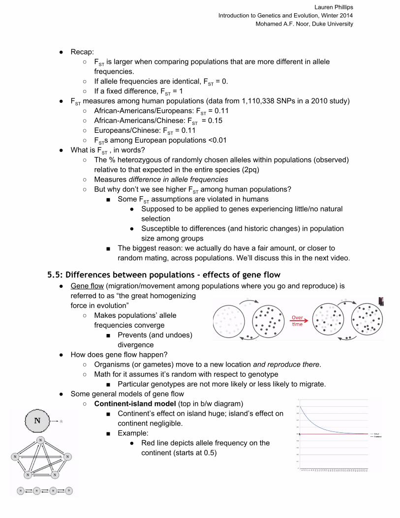
5.5: Differences between populations - effects of gene flow Gene flow (migration/movement among populations where you go and reproduce) is

referred to as “the great homogenizing force in evolution”

Makes populations’ allele frequencies converge

Prevents (and undoes) divergence

How does gene flow happen? Organisms (or gametes) move to a new location and reproduce there. Math for it assumes it’s random with respect to genotype

Particular genotypes are not more likely or less likely to migrate. Some general models of gene flow

Continentisland model (top in b/w diagram) Continent’s effect on island huge; island’s effect on

continent negligible. Example:

Red line depicts allele frequency on the continent (starts at 0.5)



Blue line depicts allele frequency (starts at 0.5) Migration rate = 1% 500 generations Island allele frequency converges onto the continent value.

Island model Multiple populations affecting each other’s

allele frequencies (middle in b/w diagram) Example:

4 islands exchange genes with each other:

p = 0.9 p = 0.65 p = 0.35 p = 0.1

Again, migration rate = 1% and this is modeled over 500 generations.

All four converge on the mean value of the islands. There is also the steppingstone model (bottom in b/w diagram we

won’t really discuss this one much) Relevant variables: What affects the speed of convergence how fast the allele

frequencies become similar? Migration rate how many migrants move

More migration leads to bigger changes How different the allele frequencies are

More different allele frequencies causes bigger change. Number of generations is obviously important too even low levels of migration

over long period could erase all divergence. There are assumptions here, including

Migration rates are symmetric Migration rates are independent of genotype Migration rates involve no difference in fitness

An example of application: Glass & Li estimated European gene flow into AfricanAmericans

Study done in 1950s, estimated 10 generations Got PTC allele frequencies of:

Europeans p(T) = 0.455 West Africans p(T) = 0.835 African Americans p(T) = 0.697

Did some very simple math (which we won’t get into here) and were able to give a pergeneration estimate of 0.0358 (3.58%)

Total contribution: ~31%



PTC = something particular individuals can taste very strongly, while other individuals cannot. Has a very simple genetic basis; given to subjects using test papers.

5.6: Inbreeding Differences in allele frequencies are often driven by patterns of gene flow and

interbreeding True when looking at different populations BUT it doesn’t have to be “between

populations” Related concept: inbreeding

Breeding between closely related individuals Capacity for dispersal often limited individuals can’t go somewhere

else to breed, so, to quote the song, they “love the one they’re with.” Changes distribution of genotypes.

An extreme form of inbreeding: selffertilization (found in some plants) Imagine this population started at 25% AA, 50% Aa, 25% aa What happens if this plant selffertilizes? (Gen 0)

AAs produce more AAs Aas produce ¼ AA, ½ Aa, ¼ aa aas produce more aas

Gen 1: After 1 generation, genotype frequencies become 37.5% AA, 25% Aa, 37.5% aa

Again, a reduction in heterozygotes relative to what we saw previously Gen 2: 43.75% AA, 12.5% Aa, 43.75% aa And so on … Eventually you’ll reach 50% AA / 50% aa / no heterozygotes Every generation, the heterozygote fraction goes down and feeds alleles into

homozygotes creates “pure breeding” lines How do we quantify inbreeding?

Inbreeding (even if not selffertilizing) reduces the percentage of heterozygotes Feeds alleles into homozygotes

Reduction in % heterozygotes from HW expected quantifies inbreeding We’ll use something called Wright’s inbreeding coefficient (F)

Very similar to FST F ranges from 0 to 1

0 = at HW expectation for % heterozygotes 0 < F < 1 = somewhat fewer heterozygotes than predicted 1 = no heterozygotes

F = HW predicted 2pq % observed heterozygotes HW predicted 2pq

Example: You’re studying a population with the genotypes: AA (553), Aa (294), aa (153) → total 1000

AA = 0.553 p(A) = 0.7



Aa = 0.294 q(a) = 0.3 aa = 0.153

HW expectation: AA (0.49), Aa (0.42), aa (0.09) F = (0.42 0.294)/0.42 = 0.30 → pretty severe inbreeding

Another example to try, involving real genotypes on Croatian islands (and skipping the genotypecount step):

AA: 0.8136 p(A) = 0.9 Aa: 0.1728 q(a) = 0.1 aa: 0.0136

HW: p2 + 2pq + q2 0.81 + 0.18 + 0.01

F = (0.180.1728)/0.18 = 0.04 estimated inbreeding coefficient So what is the difference between inbreeding F and FST?

Both based on same principle Seeing fewer heterozygotes than HW prediction Indicates nonrandom mating Symptom of Wahlund effect

Apply inbreeding F when looking at individuals within one population

Apply FST when quantifying the difference between populations How is this calculation used?

Association between inbreeding and health/disease example: effects on fetal growth in Beirut

Patterns of gene flow between social classes example: consanguineous marriage between

social/occupational class boundaries in Pakistan Other cultural effects on patterns of breeding

example: consanguinity in Spain and its socioeconomic, demographic and geographic influences

But isn’t inbreeding bad? By itself, inbreeding only changes the distribution of alleles among genotypes

it does not make any alleles “go away.” Nonetheless, many know of inbreeding depression this requires natural

selection as well as inbreeding. Populations often harbor many individually rare recessive mutations

A few new detrimental mutations each generation Because they’re both rare and recessive, their effects are often not

seen. But if two relatives mate:

They’re likely to have the same recessive mutation. They’re more likely to produce homozygous offspring.

Effects of this are often seen in dog breeds:



Breeding of relatives has created many dog breeds that have maintained “desirable” qualities such as behavior, appearance, etc.

The inbreeding F in some dogs > 0.5 (which is unusual) F = 0.7 in some poodle varieties A UPenn study showed 75% of puppies with inbreeding F > 0.67

die within 10 days King Charles spaniels get syringomyelia (skull too small for

brain) Other dogs connected to problems:

Boxers high epilepsy Pugs breathing problems Bulldogs often cannot mate or give birth unassisted Mastiffs, St. Bernards, Great Danes hip dysplasia Again, what’s happening is you’re eliminating

heterozygotes and by making dogs homozygous, the recessive bad effect becomes visible.

Week 6: Natural selection and genetic drift

6.1: Natural selection fundamentals What is natural selection?

“preservation of favourable variations and the rejection of injurious variations” Darwin (1859)

He presented his idea simultaneously with A.R. Wallace. Their emphases differed, but both are correct:

Darwin: emphasized competition within species Wallace: emphasized environmental pressures

Requirements for evolution by natural selection Variation in traits Heritability of traits Trait variants affect survival or reproduction

Quantitative traits vs. single locus We already discussed selection in the context of heritability: H = R/S

How much genetic component of variation there is dictates amount of selection’s response

Response often from change in allele frequencies at multiple loci Can also be studied at a single locus or gene

What does selection do to alleles at individual loci Affects abundance of particular genotypes

Example: AA: good, Aa: good, aa: “less good” (dead?) Affects frequency of alleles in population

The result of the scenario above is fewer a alleles remaining in the population



Dominance of alleles matters for selection. If a were dominant, Aa would ALSO be dead.

So, how often does natural selection happen in humans? Strong selection in humans single loci

Spontaneous bad mutations are common Half of pregnancies are never detected because they spontaneously

abort very early. Half of spontaneous abortions result from genetic problems

thus, ¼ of all human fertilizations are immediately eliminated by natural selection.

Weaker selection in humans single loci Historically, all humans were lactoseintolerant as adults. Estimates suggest the lactoseintolerant have about 5% fewer kids than

lactosetolerant. After a new mutation arose, most people are now “lactase persistent”

(lactosetolerant) as adults What is the effect of 5% more kids? Effect can be simulated with

AlleleA1 software fitness of AA (intolerant) = 0.95 fitness of Aa and aa (tolerant) = 1.00 Time: 5000 years All were AA and then new mutation a arose in Africa

5,000 years ago. The simulator finds only 20% of adults are

lactoseintolerant today not far from what we actually see in human populations.

Weak selection over long periods of time can lead to very big changes in allele frequencies.

Darwin actually suggested this. Selection uses “relative fitness” of genotypes

In lactase example: AA: 0.95, AA: 1.00, aa: 1.00 AA has 5% fewer kids successfully on average than aa or Aa

Being “selected against” doesn’t mean something is bad by itself just not as good as the alternative.

Humans survived for a long time as AA (lactose intolerant) A silly music analogy: A new mutation is like a newly released cover of a

previously released song. The original cover was popular/successful

“I Love Rock & Roll” originally by the Arrows, 1975 The cover may be more successful spreads (via sales) and causes

everyone to forget the original.

http://faculty.washington.edu/herronjc/SoftwareFolder/AlleleA1.html



People are more likely to know “I Love Rock & Roll” from Joan Jett and the Blackhearts’ 1982 cover.

Or the cover may be less successful around briefly, then it dies off. Let us never speak of Britney Spears’ 2002 cover again.

An example: Let’s say BB produces average 3.2 surviving offspring; Bb produces 3.0; and bb produces 2.4.

The most fit genotype is BB it does the best job of replacing itself Call it 100% of maximum fitness = w(BB) = 1.00 Others are a percentage of this maximum:

w(Bb) = 3/3.2 = 0.94 (6% less fit than BB) w(bb) = 2.4/3.2 = 0.75 (25% less fit than BB)

What are the effects on HardyWeinberg? Assume all aa individuals die at age 10. At age 8: AA: 490, Aa: 420, aa: 90. Is this population at HW? Yes.

p(A) = 0.70 At age 25: AA: 490, Aa: 420, aa: dead.

Selection altered genotype frequencies, resulting in deviation from HW. It also altered allele frequencies: p(A) = 0.769

Is aa gone for good? NO. Assuming random mating, we use the new allele frequencies to predict

0.054 aa offspring

6.2: Types at single loci Selection and dominance

In previous example, all adult aa die. We’re changing the allele names from A and a to M and N (to avoid lowercase

letters implying recessiveness) Example 1: Which allele is dominant/recessive here?

w(MM) = 1.00; w(MN) = 1.0; w(NN) = 0 MM and MN have same relative fitness, so it must be N that’s recessive The recessive form is detrimental (“bad”) in this case but it isn’t

always. Example 2: w(MM) = 1.00; w(MN) = 0; w(NN) = 0

What allele is dominant? N. What will this selection do differently?

Selection likely to be much quicker, since you’re eliminating ALL N from the population at once not just a subset of N.

With a dominant detrimental, the heterozygotes also respond to select.

Example 3: ww(MM) = 1.00; w(MN) = 0.5; w(NN) = 0 Which one is dominant? Neither no homozygous has the same relative

fitness as this heterozygous. This is a case of “no dominance.”



In all three cases, we assume NN is the worse one this is called directional selection.

In this case, selection pushes toward elimination of the N allele over time, while MM remains perfectly healthy.

Example 1 is slow to eliminate Ns; example 2 is fast to eliminate them, and example 3 it would be intermediate.

Effect of dominance with directional selection (simulated in AlleleA1): Dominant detrimental

w(MM) = 1.0, w(MN) = 0.5; w(NN) = 0.5 Since no Ns can hide, they go away pretty quickly this results in a

sharp curve. Recessive detrimental

w(MM) = 1.0, w(MN) = 1.0, w(NN) = 0.5 NNs are removed pretty readily, but MNs survive this results in a more

gradual curve, especially near the end. Some Ns remain in the population for a fairly long period of time. This is the case for most “bad” mutations, and many known genetic

diseases, such as TaySachs and cystic fibrosis they’re maintained by carriers, and selection is inefficient for getting rid of them.

This is also the case in the lactoseintolerance example we discussed earlier.

Types of direction on a single locus: Directional selection one allele eventually replaces the other, eliminating variation.

w(AA) ≤ w(Aa) ≤ w(aa) OR w(AA) ≥ w(Aa) ≥ w(aa) Recessive detrimental: w(AA) = 1.00; w(Aa) = 1.00; w(aa) = 0 → all AA No dominance (intermediate dominance): w(AA) = 1.00; w(Aa) = 0.5; w(aa) = 0

→ all AA w(AA) = 0.1; w(Aa) = 0.2; w(aa) = 1.00 → all aa Lactase persistence: w(AA) = 0.95; w(Aa) = 1.00; w(aa) = 1.00 → aa

(lactosetolerant) May not happen in real life because lactase is available

overthecounter. Heterozygote advantage (or overdominance)

The most fit genotype is the heterozygote (Aa) w(AA) = 10.85; w(Aa) = 1.00; w(aa) = 0.05

One allele does NOT replace the other variation is maintained Leads to a stable equilibrium

Both alleles are retained in the population Alleles go to equilibrium frequencies. If they’re not at that equilibrium frequency, they go back to it (oscillate

around that point). Example: Sicklecell anemia and malaria resistance.

Malaria a big threat for much of the developing world



~4% chance of dying from malaria in subSaharan Africa. Mosquito bites transmit Plasmodium protozoa, which causes

malaria Sicklecell anemia is a recessive genetic disease (aa)

Sickle cells die faster than normal red blood cells They deliver less oxygen to cells Symptoms include chronic pain and fatigue.

If heterozygote (Aa), it’s called sicklecell trait These people are usually healthy but cells may sickle during

intense physical exertion. They’re also more resistant to malaria!

Previously thought that the invasion, growth, development of Plasmodium may be reduced in Aa blood cells

1 recent study suggests Aas are more tolerant to sicklecell symptoms but retain the same infection load.

Another recent study suggests infected Aa cells are more likely to be eliminated by the spleen, since being Aa eliminates one defense of Plasmodium.

Thus, sickle cell exhibits a heterozygote advantage in some populations.

SubSaharan Africa Sample fitness

AA susceptible to malaria w(AA) = 0.85

Aa generally fine w(Aa) = 1.00

aa sicklecell anemia disease w(aa) = 0.05

What would be the fate of the a allele if it arose as a mutation in the AA population?

AlleleA1 simulation shows it would rise slightly and come to an equilibrium, stabilizing around a frequency of 0.136.

Let’s try the math ourselves: q(a) = 1w(AA)

(1w(aa)) + (1(w(AA)) q(a) = 0.15/(0.95 + 0.15) = 0.15/1.1 = 0.136

Heterozygote disadvantage (or underdominance) there aren’t many good examples of this. It’s unstable could be argued to maintain variation, but only under unrealistic circumstances.

The least fit genotype is the heterozygote w(AA) = 1.00; w(Aa) = 0.2; w(aa) = 0.5

This leads to an unstable equilibrium (0.27272727) If starting below equilibrium, you go to a loss.



If starting above equilibrium, you go to a fixation and lose the other allele entirely

If starting (and staying) at equilibrium, alleles persist but this is very unlikely in a real population.

Frequencydependent selection (specifically, the negative variety) maintains variation.

Previous examples assumed fitness was independent of the rest of the population.

Sometimes it’s better to be “rare” fitness may depend on your relative abundance.

But being “better” makes you become more common. This eventually leads to equilibrium. Example: sex ratio

Sex (male vs. female) is determined genetically in many species. In mammals, XXXY means they’re mostly locked in to 5050

ratio by transmission. In other species, alleles at a gene cause an individual to become

male vs. female. If females are rare, is it better to produce male or female offspring?

The rare type, because you’re more likely to mate. Would selection favor male or female allele?

Outcome of negative frequencydependent selection When rare, allele has advantage When common, allele has disadvantage Genetic variation is maintained in the population If you have 2 alleles, what do you predict the equilibrium allele

frequency to be? Assuming it’s symmetric, 50% (1/number of alleles) What if a third allele is introduced into the population?

⅓ All of these singlelocus selection types affect genotype and allele frequencies, but act

on phenotype.

6.3: Types acting on traits Natural selection can be studied in the context of either quantitative traits or a single

loci Darwin thought of natural selection in the context of variation of traits (as many

breeders do). It can also be studied in the context of phenotypes, as in our discussions of

heritability Don’t necessarily need to know the underlying genes to infer the type of

selection operating. We’ll look at three types of selection,

inferred from phenotypes:



directional selection favors individuals at one end of the distribution This causes a change in the mean of the population over time. Example: pink salmon weight over time, smaller and smaller salmon

(more likely to be thrown back by fishermen) were caught. not the same as the previous “directional selection” we discussed.

stabilizing selection favors individuals with intermediate values No change in mean, but you lose some of the extremes Not the same as overdominance that involves looking at a single gene;

here, we’re looking for a pattern in phenotypes In 1898, a New Englander named Bumpus was interested in sparrows.

When a huge ice storm killed a bunch of birds, he brought in 136 that weren’t doing too well 64 died, 72 lived.

He found the mean weight of the survivors was the same as the mean of the dead.

But all birds weighing more than 28g or less than 23g died. An example in humans: birth weight

disruptive selection favors individuals with extreme values (at both ends of the distribution)

No change in the mean, but loss of intermediate phenotypes greater variance over times

The exact opposite of stabilizing selection Example: female African finches peaks in beaksize chart corresponds

with specialization to eat two types of sedge seeds. Intermediate birds aren’t as good at either, and aren’t as fit.

Final thoughts: Is selection “good” or “bad” for a population? Natural selection preferentially reduces/eliminates “bad” genotypes. The average fitness of all individuals remaining in the population after selection

goes up. Since bad alleles are removed, simple directional selection gives

longterm improvement to the population. Fisher’s fundamental theorem of natural selection the rate of increase in

fitness is equal to the genetic variance in fitness. If there’s a lot of variance in fitness, you’ll see large step changes.

6.4: Case studies and examples Case studies of mimicry

Mimicry: organisms evolving to resemble another. It’s presumed to be adaptive when the “model” species has a warning

coloration that causes predators to fear or avoid it this makes the other organism less likely to be harassed or eaten.

Two general types: Batesian mimicry the mimic isn’t dangerous, but the model is derives

advantage only for the mimic



example: nonvenomous king snake resembles venomous coral snake

Müllerian mimicry a lot of dangerous species evolving to look like one another, thus deriving a mutual advantage.

example: tropical butterflies evolving to look like another type in their specific local population.

Variation across space and time Ecogeographic rules patterns of variation within or among species that

correlate with geography. Bergmann’s rule animals tend to be bigger in cold environments or

high latitudes. Why might this be? Perhaps it increases volume but not surface

area, which might help hold in heat. Allen’s rule animals tend to have shorter appendages in cold

environments. Again, could be attributed to heat loss Example: polar bears’ shorter ears; house sparrow bill size

Gloger’s rule animals tend to be more heavily pigmented in high humidity

typically true near the Equator may be related to bacterial activity may also be true in humans, but the evidence to suggest is far

from perfect. Here we’ve been looking at genotypes, but the same types of geographic

patterns can be seen in alleles, too Drosophila pseudoobscura alleles on third chromosome we’ll focus on

one called Arrowhead (AR) Dobzhansky found a correlation between AR frequency and

altitude (increased as the altitude of populations’ homes increased).

Also patterns based on humidity and latitude There are also temporal patterns with alleles:

D. pseudoobscura’s AR becomes less abundant as it gets hotter over the year.

Sacrifice for family members Why do some animals sacrifice their ability to reproduce to help others, often relatives?

Darwin: “Selection may be applied to the family, as well as the individual, and may thus gain the desired end.”

An example: If you’re selfish and just have your two kids, you pass on half of your

genetic information to each offspring and your alleles live on.



If you have no kids, nothing gets passed on and your alleles die with you.

If you have four sisters each of whom shares half your genetic information and they have two kids each, your nieces each share a quarter of your genetic information.

Counterintuitively, it’s actually more beneficial for you to die in the process of helping your sisters have offspring that survive than it is for you to just have your two kids. Your alleles live on twice as well.

Kin selection evolutionary strategy that favors the reproductive success of an organism’s relatives, even when at a cost to the organism’s own reproduction.

Evolutionary biologist J.B.S. Haldane asked if he’d give his life to save a drowning brother, said “No, but I would to save two brothers or eight cousins.”

A possible example: the Belding’s ground squirrel and the alarm calls it uses in the event of imminent threat.

Dangerous for the caller, which stands up and thus becomes more conspicuous

Possibly evolved/spread to help relatives Females do alarm call more frequently when relatives are

around.

6.5: Genetic drift and sampling error One of HardyWeinberg’s assumptions is an infinite or near infinite population size. Since that’s generally not going to happen, there’s bound to be some sampling error this is called genetic drift.

Contrasting natural selection and genetic drift: Natural selection is predictable

Some genotypes have a higher fitness Higher fitness leads to more offspring Genotypes become overrepresented

If the fitness is known, then change by natural selection is predictable. But not all evolutionary change is …

Because species have a finite number of individuals, random chance matters. Say you’ve got a bag of marbles, half brown and half blue.

If you picked out exactly four marbles to start a new bag, how many of each color would you get?

Only about a 12% chance of getting the same color on all four What if you picked out two?

There’s now a 50% chance of getting all the same color. That last example illustrates sampling error:

Picking 4 marbles is likely to get you roughly “right” proportions (the proportions of the original pool).



Picking 2 is NOT likely to get you roughly right proportions. By picking more, you get a more representative sample of the original

pool The same principle applies in nature:

Populations are not infinite Frequently, a small (not perfectly representative) sample of gametes

form the next generation. Allele and genotype frequencies change

The effect compounds over time. Sampling error is random in direction over one generation

Assuming there is more than one allele, any allele is about equally likely to increase or decrease in frequency in one generation by sampling error.

If p=0.6, it’s about equally likely to be less than or greater than 0.6 (but very unlikely to be exactly p=0.6 again)

Allele frequency “drifts” due to sampling error thus, genetic drift. Small changes are likely; big changes are possible but unlikely

If you tossed a coin 10 times (similar to p=0.5) you might get heads on 5 tosses.

Getting more or less than 5 is equally likely It’s very unlikely you’ll get 01 heads, or 910

(Chance of hitting heads all 10 times is 1/1000) Same concept applies to populations.

Original population has p(A)= 0.6 At right is the probability of p(A) after

1 generation (assuming 10 diploid offspring)

The magnitude of the change compounds and relates to the population size.

Greater changes occur in the allele frequency if the sample (population) is smaller.

Here, we have a population size of about 400, A1 starts at 0.5, and we’re seeing random changes over eight populations.

The little green tuning fork thing on the left side is the approximate average size of a change in one generation.

When we reduce population size to 40, the step size of changes is much bigger.



And at a population size of 4? All variation is lost and the step size is very large.

How big are the individual steps (on average)? Variance in allele frequency due to one generation of drift

= (pq)/(2N) p and q are allele frequencies; N is population

size. 2N used because these are diploid organisms

Standard deviation is (slight over)estimate of average allele frequency change in one generation: √ (pq)/(2N)

in other words, the square root of the variance. For N = 4, p = 0.5, q = 0.5, average change estimate

~0.18 Likely to go to p=0.68 or p=0.32 average; could

be more or less For N=40, p=0.5, q=0.5, average change estimate ~0.06 For N=400, p=0.5, q=0.5, average change estimate ~0.02

Takeaways from this lecture: Drift is strongest in small populations Drift is neither predictable in direction in one generation nor exactly replicable in

degree You can get different results under the exact same conditions

Drift can cause big changes in allele frequency over time.

6.6: Sampling error over many generations Longterm effects of drift

Start with variable population, 2 alleles (example: p(A) and q(a) are both 0.5) After many, many generations, p(A) = 0 or 1 Why? Once you get to 0 or 1, there’s no variation because one allele is

completely gone so you can’t “drift” back What if you start with a variable population, 2 alleles (p(A) = 0.6, q(a) = 0.4)?

Is population likely to be fixed for A or a over time? Analogy: If a blindfolded man starts walking aimlessly from dead center

between 0 and 1, he’s about equally likely to hit one as the other. But if he starts closer to 1 than 0, he’s more likely to reach 1.

Probability of a longterm outcome is predictable In one generation, it’s roughly equally likely for an allele’s frequency (p(A)) to

go up and down But longterm “loss” or “fixation” of an allele is more predictable

If p(A) = 0.5, equally likely if p(A) < 0.5, more likely that allele will be lost if p(A) > 0.5, more likely that allele will be fixed

Probability of eventual fixation of A = p(A).



If we do 4 sample runs in AlleleA1 with p(A) = 0.75 and a population size of 100, it hits 1 three out of the four times.

Still some chance for an allele to get lost despite starting out abundant (that’s what happened in the other sample run).

So far, we’ve just looked at what happened in one population. What happens if we look at whole species, including some isolated populations?

If all 4 populations of Galapagos land snail started with p(A) = 0.75: What would the allele frequencies be in the populations many years

later? We’d expect, on average, three of the populations to be fixed

and one to be lost. What would the average p(A) across all populations be many years

later? It’s still 0.75 across the species the allele still exists in some

populations despite dying out in others. Points to remember

Drift eventually leads to allele fixation or loss in every population Starting allele frequency p(A) is a longterm probability of the allele’s fixation

(1p(A)) is a longterm probability of allele’s loss In a species with many isolated populations, the overall species retains

variation with the same p(A), despite individual populations’ fixation/loss. Interaction of genetic drift and natural selection: Can genetic drift make “bad” alleles

spread (or even be fixed)? If the population size is small (i.e. drift is strong), genetic drift can sometimes

counteract weak selection to spread or fix a “bad” allele. Won’t always counteract selection, because drift is random in direction

in each generation. May push in the same direction, too.

6 simulations of strong drift and weak selection p(A) = 0.5, w(AA) = 0.98, w(Aa & aa) = 0.0, N = 100

AA is a recessive detrimental only 0.02 from other genotypes 1 of the 6 actually loses little a the better allele! This is a case

when genetic drift overpowers selection. What happens if the population size is larger (1,000), resulting in weaker drift?

6 simulations (all numbers but population size are same as above) Consistent trajectory of decrease that, if we followed it out

enough, would eventually end in loss of A. More noise than the previous example.

An extreme case of genetic drift: founder effects strong genetic drift when a new population is established by a very small number of individuals from a larger population.

Often associated with colonizing islands



Sometimes causes spread (or fixation) of even detrimental alleles, since drift is strong.

Cause diseases or traits to be common in certain human populations. Polydactyly in the Amish TaySachs disease in Ashkenazi Jewish

Half the Ashkenazis trace their ancestry to four women. Huntington’s disease in Mauritius Red hair among the Irish

6.7: Rate of neutral molecular evolution Are longterm effects of mutations and genetic drift predictable?

New mutations arise at some rate Mutations in some parts of genome are “neutral” have no effect on fitness

Might spread or be lost by drift Can we predict the rate at which they arise and spread to fixation?

Ancient population sizes unknown Let’s try breaking the problem up into pieces:

Mutations arise (we’ll call the rate μ) Could be mutations per year or per generation we’ll use “per year”

here. Example: μ = 1 x 109 mutations per year per base pair studied

In bigger populations, you’re more likely to get a mutation (just because there are more alleles present)

Rate of getting new mutations = 2Nμ 2N is because these are pairs (diploid)

The mutation must then also fix by drift What’s the probability of fixation of a new mutation in diploids?

Probability of new mutation arising x probability of new mutation fixing = 2Nμ + 1/(2N) → μ

Large populations have more chance of a mutation arising, but a smaller chance it will fix

The rate of neutral molecular evolution does not depend on population size.

How do we apply this calculation? Mutation rate for human pseudogenes is roughly 1 x 109 mutations per

year per base pair pseudogene = a gene that is no longer functional, so any

mutations within it are going to be neutral. Let’s say we want to know the divergence time between humans and

mouse lemurs Sequence a pseudogene and see 150 base differences in 1,000

base pairs between the two. Not unusual.



We can use this to determine how far back the two shared a common ancestor

1 x 109 mutations per year per base pair 1 x 106 mutations in 1,000 bp/year (1,000 times greater) invert numbers: so 106 years/1 mutation in 1,000 bp

see 150 mutations: 150 mutations x 106 years/mutation = 1.5 x 108 years total divergence

BUT, two branches, so we divide by two: 7.5 x 107 years to ancestor (75 million years)

Here’s another one to try: time to ancestor for humans and tamarin 1 x 109 mutations per year per base pair Screened 10,000 bp of sequence Found 860 mutations (1 x 109) x 10,000 = (1 x 105) mutations in 10,000 bp/year

invert numbers: 105 years/1 mutation in 10,000 bp 860 mutations x 105 years/1 mutation = 8.6 x 107 years

total divergence two branches → 4.3 x 107 to ancestor (43 million years)

If you’re interested, http://timetree.org allows you to look up more molecular estimates of divergence times between species.

NEXT WEEK … Nucleotide variation within and between species. Some mutations are advantageous; many mutations are bad How much of the genome actually evolves solely via mutation and genetic drift

(“neutrally”)? Two schools of thought since the 1960s:

Neutralists most nucleotide variation within and between species is neutral

Selectionists very little nucleotide variation is neutral

http://timetree.org/

Week 5: The Hardy-Weinberg equilibrium, population ... · Lauren Phillips Introduction to Genetics...

Documents

Transcript of Week 5: The Hardy-Weinberg equilibrium, population ... · Lauren Phillips Introduction to Genetics...