Abstraction Layers for

Scalable Microfluidic Biocomputers

William Thies1, John Paul Urbanski2,Todd Thorsen2, and Saman Amarasinghe1

1 Computer Science and Artificial Intelligence Laboratory2 Hatsopoulos Microfluids LaboratoryMassachusetts Institute of Technology

{thies, urbanski, thorsen, saman}@mit.edu

Abstract. Microfluidic devices are emerging as an attractive technol-ogy for automatically orchestrating the reactions needed in a biologicalcomputer. Thousands of microfluidic primitives have already been inte-grated on a single chip, and recent trends indicate that the hardwarecomplexity is increasing at rates comparable to Moore’s Law. As in thecase of silicon, it will be critical to develop abstraction layers—such asprogramming languages and Instruction Set Architectures (ISAs)—thatdecouple software development from changes in the underlying devicetechnology.Towards this end, this paper presents BioStream, a portable languagefor describing biology protocols, and the Fluidic ISA, a stable interfacefor microfluidic chip designers. A novel algorithm translates microflu-idic mixing operations from the BioStream layer to the Fluidic ISA. Todemonstrate the benefits of these abstraction layers, we build two mi-crofluidic chips that can both execute BioStream code despite significantdifferences at the device level. We consider this to be an important steptowards building scalable biological computers.

1 Introduction

One of the challenges in biological computing is that the laboratory protocolsneeded to carry out a computation can be very time consuming. For example, a20-variable 3-SAT problem required 96 hours to complete [1], not counting theconsiderable time needed for setup and evaluation. To automate and optimizethis process, researchers have turned to microfluidic devices [2–10]. Microfluidicsoffers the promise of a “lab on a chip” system that can individually controlpicoliter-scale quantities of fluids, with integrated support for operations such asmixing, storage, PCR, heating/cooling, cell lysis, electrophoresis, and others [11–13]. Apart from being amenable to computer control, microfluidics drasticallyreduces the volumes of samples, thereby reducing costs and improving capturekinetics. Using microfluidics, DNA hybridization times can be reduced from 24hours to 4 minutes [10] and the number of bases needed to encode informationcan be decreased from 15 bases per bit to 1 base per bit [1, 8].

Computational problem

Biology expert

Microfluidics expert

������� �� �� �Max-clique graph

Biology protocol����� � ����� �

, oligo generation

Concentrations of DNA, buffer, etc.

Selection and isolation steps

Microfluidic chip operations

Connectivity and control logic

Locations of inputs, fluids, beads, etc.

Calibration and timing

chip 12

3

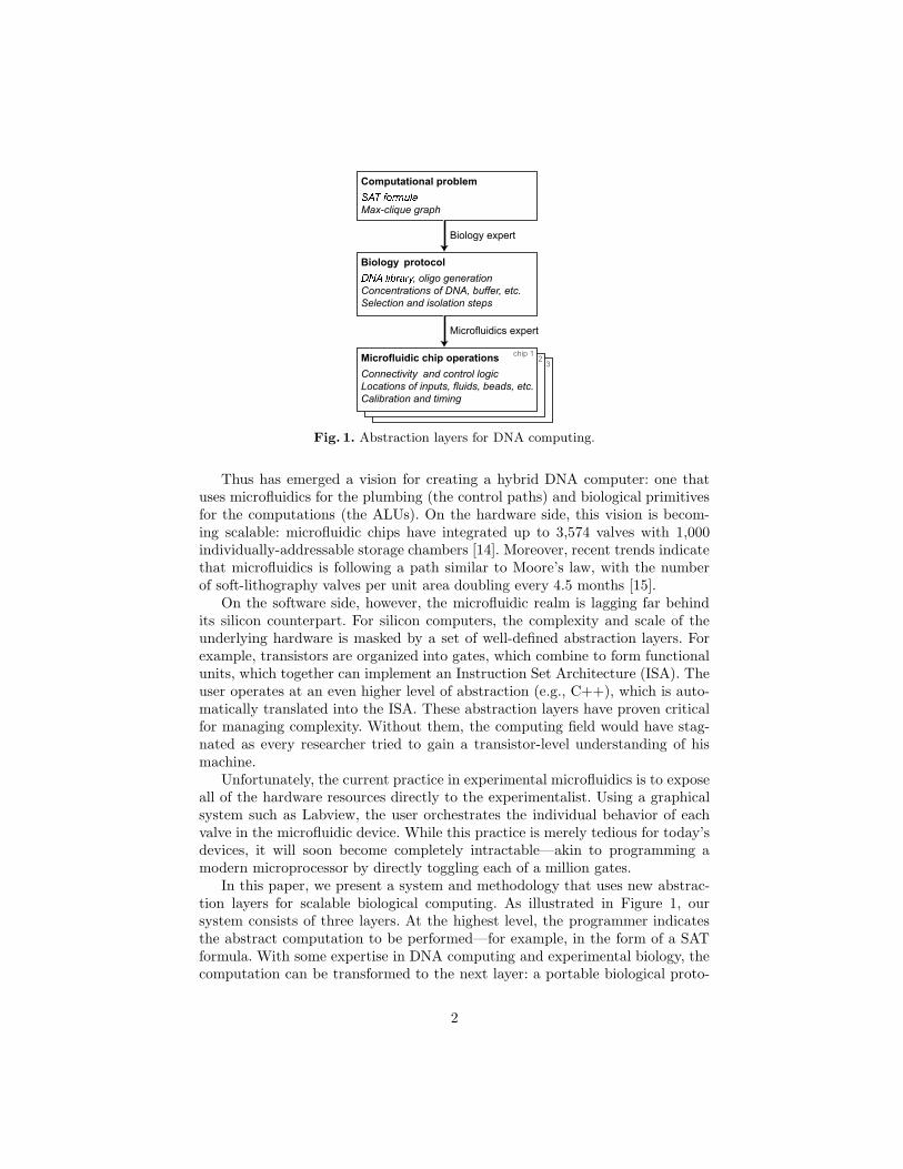
Fig. 1. Abstraction layers for DNA computing.

Thus has emerged a vision for creating a hybrid DNA computer: one thatuses microfluidics for the plumbing (the control paths) and biological primitivesfor the computations (the ALUs). On the hardware side, this vision is becom-ing scalable: microfluidic chips have integrated up to 3,574 valves with 1,000individually-addressable storage chambers [14]. Moreover, recent trends indicatethat microfluidics is following a path similar to Moore’s law, with the numberof soft-lithography valves per unit area doubling every 4.5 months [15].

On the software side, however, the microfluidic realm is lagging far behindits silicon counterpart. For silicon computers, the complexity and scale of theunderlying hardware is masked by a set of well-defined abstraction layers. Forexample, transistors are organized into gates, which combine to form functionalunits, which together can implement an Instruction Set Architecture (ISA). Theuser operates at an even higher level of abstraction (e.g., C++), which is auto-matically translated into the ISA. These abstraction layers have proven criticalfor managing complexity. Without them, the computing field would have stag-nated as every researcher tried to gain a transistor-level understanding of hismachine.

Unfortunately, the current practice in experimental microfluidics is to exposeall of the hardware resources directly to the experimentalist. Using a graphicalsystem such as Labview, the user orchestrates the individual behavior of eachvalve in the microfluidic device. While this practice is merely tedious for today’sdevices, it will soon become completely intractable—akin to programming amodern microprocessor by directly toggling each of a million gates.

In this paper, we present a system and methodology that uses new abstrac-tion layers for scalable biological computing. As illustrated in Figure 1, oursystem consists of three layers. At the highest level, the programmer indicatesthe abstract computation to be performed—for example, in the form of a SATformula. With some expertise in DNA computing and experimental biology, thecomputation can be transformed to the next layer: a portable biological proto-

2

col for performing the computation. The protocol is portable in that it does notdepend on the physical implementation of the protocol; for example, it specifiesfluid concentrations but not fluid volumes. Finally, the bottom layer specifies theoperations needed to execute the protocol on a specific microfluidic chip. Eachmicrofluidic chip designer provides a library that translates an abstract protocolinto the specific sequence of valve actuations needed to execute that protocol ona specific chip.

These abstraction layers provide many benefits. Primarily, by using an ar-chitecture-independent description of the biological protocol (the middle layer),the application development can be decoupled from advances in the underlyingdevice technology. Thus, as microfluidic devices come to support additional in-puts, mixers, storage cells, etc., the existing suite of protocols can run withoutmodification (much as C programs run without modification on successive gener-ations of microprocessors). In addition, the protocol layer serves as a division oflabor. Rather than requiring a heroic and brittle translation from a SAT formuladirectly to a microfluidic chip, a biologist provides a mapping to the abstractprotocol while a microfluidics expert maps the protocol to the underlying device.The abstract protocol is also perfectly suited to simulation, thereby allowing thelogical operations to be verified without relying on any physical implementation.Further, a portable protocol description could serve the role of pseudocode intechnical publications, providing a precise account of the experimental meth-ods used. Third-party protocols could be downloaded and executed (or called assub-routines) on one’s own microfluidic device.

In the long term, the protocol description language will support all of the op-erations needed for biological computing. However, as there does not yet exist asingle microfluidic device that can encompass all the functionality (preparationof DNA libraries, selection, readout, etc.), this paper focuses on three funda-mental primitives: fluid mixing, fluid transport, and fluid storage. We describe aprogramming system called BioStream (Section 2) that provides an architecture-independent interface for these operations. To show that BioStream is portable,we execute BioStream code on two fundamentally different microfluidic archi-tectures (Section 3). We also present a novel algorithm for mixing fluids to agiven concentration using the minimal number of simple on-chip mixing steps(Section 4). Our system represents a fully-functional, end-to-end demonstrationof portable software on microfluidic hardware.

2 BioStream Protocol Language

We have developed a software system called BioStream for portable microflu-idics protocols. BioStream is a Java library that virtualizes many aspects of theunderlying hardware resources. While BioStream can be targeted by a compiler(for example, a DNA computing compiler that converts a mathematical prob-lem into a biological protocol), it is also suitable for direct programming andexperimentation by biologists. As such, the language provides several high-levelabstractions to improve readability and programmer productivity.

3

�������������� �������ary

// mix fluids in arbitrary proportions

Fluid mix(Fluid[] f, double[] c);

// set precision of mixing ope ����� ions

void setPrecision(double precision);

// wait for a period before ����� ceeding

void waitFor(long seconds);

[native functions with Fluid arguments]

Microfluidic Device Microfluidic Simulator

Library

Generator

G enerate a

B ioS tream

L ibrary for an

architecture.

Simulator

Generator

G enerate a

simulated

backend for an

architecture.

Fluidic Instruction

Set Architectu�

(ISA)

// mix two fluids in eq ����������� ����� tions

void mixAndS tore(L ocation src1,

L ocation src2,

L ocation dst)

[native functions with L ocation arguments]

P����

ocol Code

Portable between microfluidic chips

supporting architecture requirements.

Declares native functions such as

I/O, sensors, agitators. �! r "$# ample:

Fluid input(Integer i);

Double camera(Fluid i);

Architectu�

Requ���� %

nts

Implemented by

H ardw &('*)Developers

Implemented by+%,�-/.�0'1)�&(2

Implemented by

P'-(0

ocol

Developers

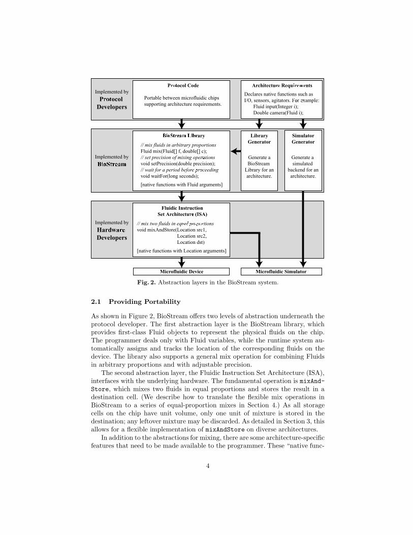
Fig. 2. Abstraction layers in the BioStream system.

2.1 Providing Portability

As shown in Figure 2, BioStream offers two levels of abstraction underneath theprotocol developer. The first abstraction layer is the BioStream library, whichprovides first-class Fluid objects to represent the physical fluids on the chip.The programmer deals only with Fluid variables, while the runtime system au-tomatically assigns and tracks the location of the corresponding fluids on thedevice. The library also supports a general mix operation for combining Fluidsin arbitrary proportions and with adjustable precision.

The second abstraction layer, the Fluidic Instruction Set Architecture (ISA),interfaces with the underlying hardware. The fundamental operation is mixAnd-Store, which mixes two fluids in equal proportions and stores the result in adestination cell. (We describe how to translate the flexible mix operations inBioStream to a series of equal-proportion mixes in Section 4.) As all storagecells on the chip have unit volume, only one unit of mixture is stored in thedestination; any leftover mixture may be discarded. As detailed in Section 3, thisallows for a flexible implementation of mixAndStore on diverse architectures.

In addition to the abstractions for mixing, there are some architecture-specificfeatures that need to be made available to the programmer. These “native func-

4

tions” include I/O devices, sensors, and agitators that might not be supportedby every chip, but are needed to execute the program; for example, special inputlines, cameras, or heaters. As shown in Figure 2, BioStream supports this func-tionality by having the programmer declare a set of architecture requirements.BioStream uses the requirements to generate a library which contains the samefunctionality; it also checks that the architecture target supports all of the re-quired functions. Finally, BioStream includes a generic simulator that inputs aset of architecture requirements and outputs a virtual machine that emulates thearchitecture. This allows full protocol development and validation even withouthardware resources.

The BioStream system is fully implemented. The reflection capabilities ofJava are utilized to automatically generate the library and the simulator fromthe architecture requirements. As described in Section 3, we also execute theFluidic ISA on two real microfluidic chips.

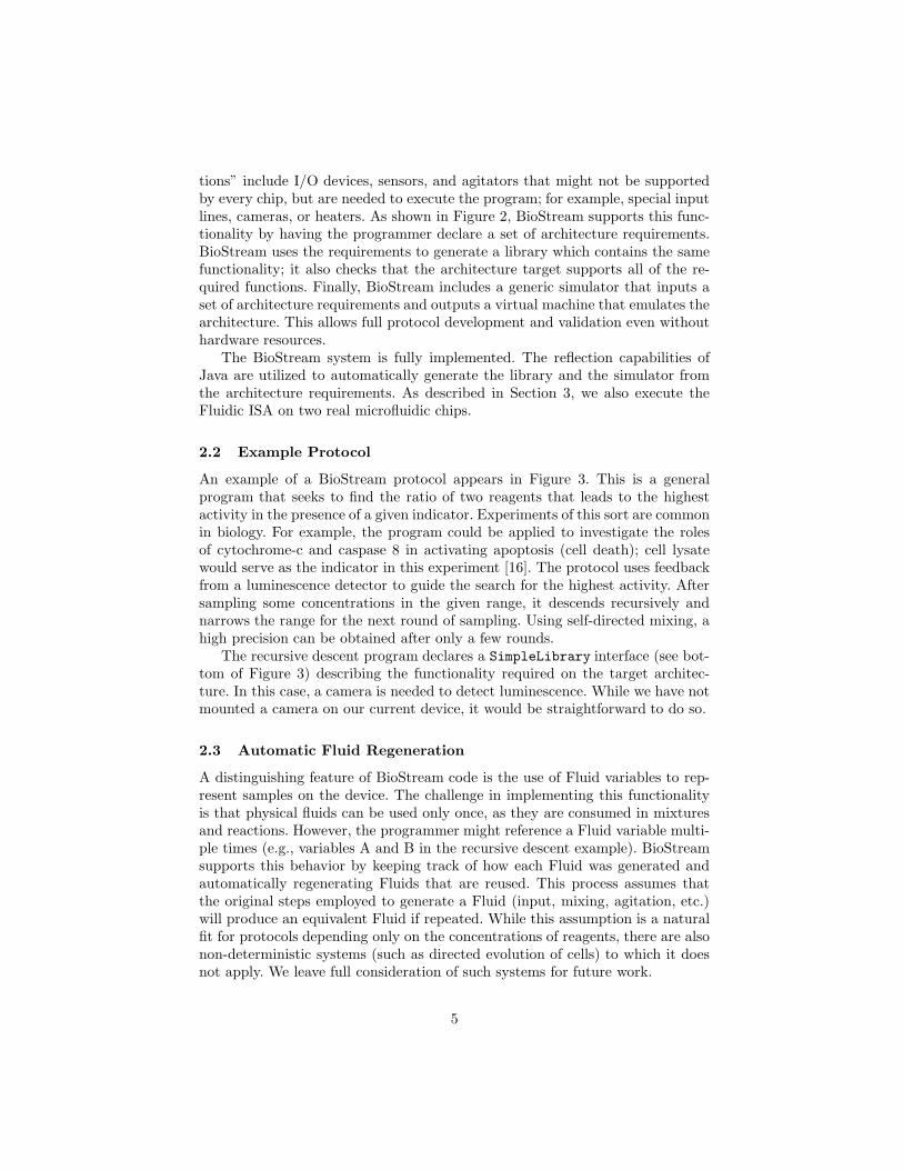
2.2 Example Protocol

An example of a BioStream protocol appears in Figure 3. This is a generalprogram that seeks to find the ratio of two reagents that leads to the highestactivity in the presence of a given indicator. Experiments of this sort are commonin biology. For example, the program could be applied to investigate the rolesof cytochrome-c and caspase 8 in activating apoptosis (cell death); cell lysatewould serve as the indicator in this experiment [16]. The protocol uses feedbackfrom a luminescence detector to guide the search for the highest activity. Aftersampling some concentrations in the given range, it descends recursively andnarrows the range for the next round of sampling. Using self-directed mixing, ahigh precision can be obtained after only a few rounds.

The recursive descent program declares a SimpleLibrary interface (see bot-tom of Figure 3) describing the functionality required on the target architec-ture. In this case, a camera is needed to detect luminescence. While we have notmounted a camera on our current device, it would be straightforward to do so.

2.3 Automatic Fluid Regeneration

A distinguishing feature of BioStream code is the use of Fluid variables to rep-resent samples on the device. The challenge in implementing this functionalityis that physical fluids can be used only once, as they are consumed in mixturesand reactions. However, the programmer might reference a Fluid variable multi-ple times (e.g., variables A and B in the recursive descent example). BioStreamsupports this behavior by keeping track of how each Fluid was generated andautomatically regenerating Fluids that are reused. This process assumes thatthe original steps employed to generate a Fluid (input, mixing, agitation, etc.)will produce an equivalent Fluid if repeated. While this assumption is a naturalfit for protocols depending only on the concentrations of reagents, there are alsonon-deterministic systems (such as directed evolution of cells) to which it doesnot apply. We leave full consideration of such systems for future work.

5

// The Recursive Descent protocol recursively // zooms in on the ratio of fluids A and B that // has the highest activity. It requires the // following setup in the laboratory:

import biostream.library.*; // - input(0) -- fluid A // - input(1) -- fluid B

public class RecursiveDescent { // - input(2) -- luminescent activity indicator

public static void main(String[] args) { // Initialize the backend to use (for example, String backend = args[0]; // an actual chip or a microfluidic simulator) // based on command-line input. SimpleLibrary lib = (SimpleLibrary)LibraryFactory. // Create an interface to the backend using the buildLibrary("SimpleLibrary", args[0]); // native functions declared in SimpleLibrary. run(lib);

}

private static void run(SimpleLibrary lib) { // Perform the protocol: int ROUNDS = 10; int SAMPLES = 5; // Set number of rounds and samples per round.

Fluid A = lib.input(new Integer(0)); // Assign names to the input fluids. Fluid B = lib.input(new Integer(1)); Fluid indicator = lib.input(new Integer(2));

double center = 0.5, radius = 0.5; // Initialize center, radius of concentration range.

for (int i=0; i<ROUNDS; i++) { // Repeat for a number of rounds: lib.setPrecision(0.1*(2*radius)/ SAMPLES); // Set absolute mixing precision to 10X // more than the granularity of sampling. double bestActivity = -1; int bestJ = -1; for (int j=1; j<SAMPLES; j++) { // Repeat across concentrations in range:

double target = center+radius* // Obtain sample of the (1-2*(double)j/SAMPLES); // target concentration. Fluid sample = lib.mix(A, target, B, 1-target);

Fluid test = lib.mix(indicator, 0.9, sample, 0.1); // Mix sample with indicator, lib.wait(30); // wait, and measure activity. double act = lib.luminescence(test).doubleValue();

if (act > bestActivity) // Remember highest activity. bestActivity = act; bestJ = j; }

center = center+radius*(1-2*(double)bestJ/SAMPLES); // Zoom in by factor of 2 around best activity. radius = radius / 2;

if (center < radius) center = radius; // If needed, move center away from boundary. if (center > 1-radius) center = 1-radius; } } System.out.println("Best activity: “ + center); // Print concentration yielding highest activity.}

interface SimpleLibrary extends FluidLibrary { // Declare devices needed by RecursiveDescent:Fluid input(Integer i); // Require array of fluid inputs.Double luminescence(Fluid f); // Require luminescence camera.

}

Fig. 3. Recursive descent search in BioStream.

6

Driving Wash Mixing Sample Inputs Storage Valves Control

fluid fluid size cells lines

Chip 1 oil N/A rotary mixer half of mixer 2 8 46 26Chip 2 air water during transport full mixer 4 32 140 21

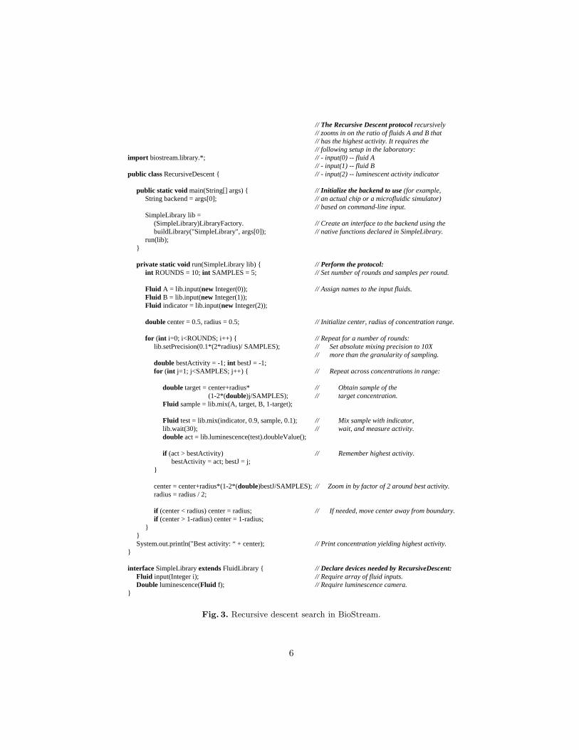
Table 1. Key properties of the microfluidic chips developed. Chip 1 provides betterisolation and retention of samples, while Chip 2 offers faster and simpler operation.

The regeneration mechanism works by associating each Fluid object with thename and arguments of the function that created it. The creating function mustbe a mix operation or a native function, both of which are visible to BioStream(the Fluid constructor is not exposed). BioStream maintains a valid bit for eachFluid, which indicates whether or not the Fluid is stored in a storage chamberon the chip. By default, the bit is true when the Fluid is first created, and it isinvalidated when the Fluid is used as an argument to a BioStream function. Ifa BioStream function is called with an invalid Fluid, that Fluid is regeneratedusing its history. Note that this regeneration mechanism is fully dynamic (noanalysis of the source code is needed) and is accurate even in the presence ofpointers and aliasing.

The computation history created for Fluids can be viewed as a dependencetree with several interesting applications. For example, the library can execute aprogram in a demand-driven fashion by initializing each Fluid to an invalid stateand only generating it when it is used by a native function. Dynamic optimiza-tions such as these are especially promising for microfluidics, as the silicon-basedcontrol processors operate much faster than their microfluidic counterparts.

3 Microfluidic Implementation

To demonstrate an end-to-end system, we have designed and fabricated two mi-crofluidic chips using a standard multi-layer soft lithography process [13]. Whilethere are fundamental differences between the chips (see Table 1), both providesupport for programmable mixing, storage, and transport of fluid samples. Morespecifically, both chips implement the mixAndStore operation in the Fluidic ISA:they can load two samples from storage, mix them together, and store the re-sult. Thus, despite their differences, code written in BioStream will be portablebetween the chips.

The first chip (see Figure 4) isolates fluid samples by suspending them inoil [17]. To implement mixAndStore, each input sample is transported from astorage bin to one side of the mixer. The mixer uses rotary flow, driven byperistaltic pumps, to mix the samples to uniformity [18]. Following mixing, onehalf of the mixer is drained and stored in the target location. While the secondhalf could also be stored, it is currently discarded, as the basic mixAndStore

abstraction produces only one unit of output.The second chip (see Figure 5) isolates fluid samples using air instead of oil.

Because fluid transport is very rapid in the absence of oil, a dedicated mixingelement is not needed. Instead, the input samples are loaded from storage and

7

��������� ������ er

� ������� 1

� ������� 2

Oil

��� �er

� ���te

� ���te

� ������� ����5 mm

�� ��� ��!e Cells

" #�$�%�&s

'�( )er

*�+�,te

*�+�,te

- & .�/ +�0e C ells

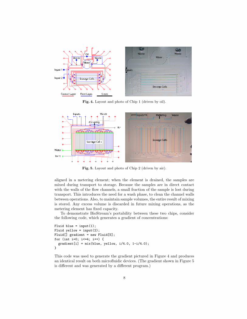
Fig. 4. Layout and photo of Chip 1 (driven by oil).

132�4te

576 8

9 :�;=<�> 4

132�>er

?A@B:t

C > D�8 2�Ee C

@GF Fs

HI@J> @B8 6ng

Inputs KML�N LGO P ng Q�R�S te

T N U�O R�V e CLGW W s

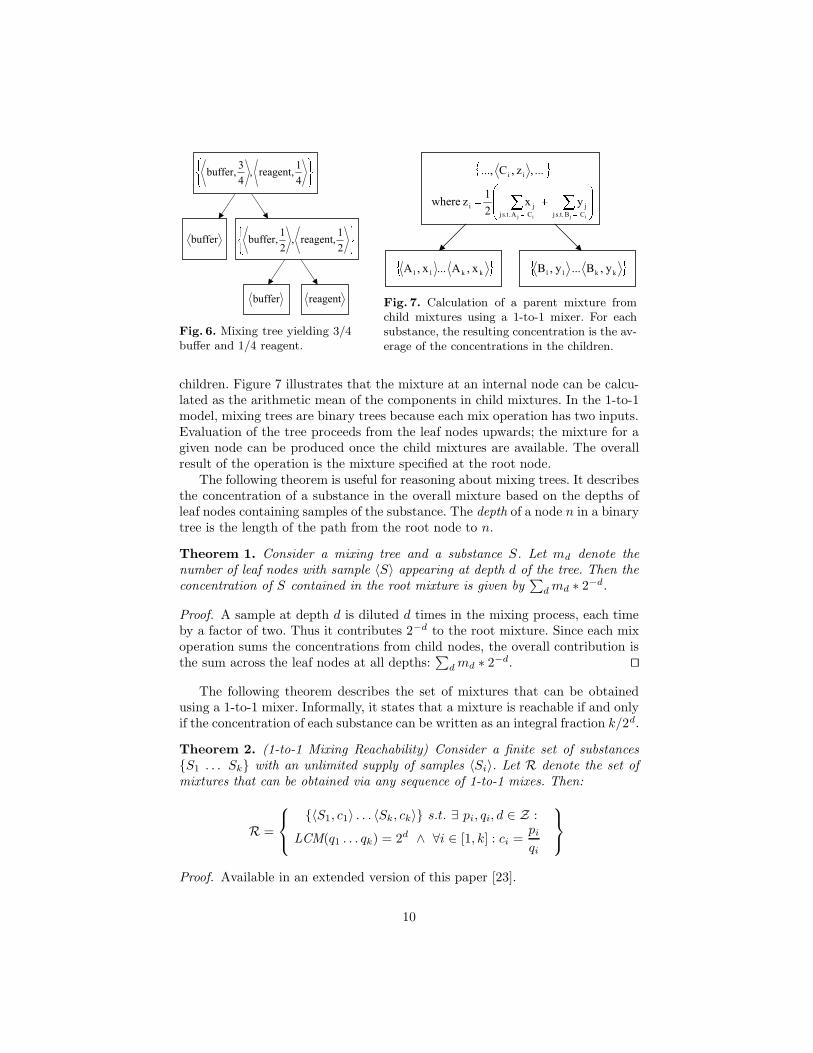
Fig. 5. Layout and photo of Chip 2 (driven by air).

aligned in a metering element; when the element is drained, the samples aremixed during transport to storage. Because the samples are in direct contactwith the walls of the flow channels, a small fraction of the sample is lost duringtransport. This introduces the need for a wash phase, to clean the channel wallsbetween operations. Also, to maintain sample volumes, the entire result of mixingis stored. Any excess volume is discarded in future mixing operations, as themetering element has fixed capacity.

To demonstrate BioStream’s portability between these two chips, considerthe following code, which generates a gradient of concentrations:

Fluid blue = input(1);

Fluid yellow = input(2);

Fluid[] gradient = new Fluid[5];

for (int i=0; i<=4; i++) {

gradient[i] = mix(blue, yellow, i/4.0, 1-i/4.0);

}

This code was used to generate the gradient pictured in Figure 4 and producesan identical result on both microfluidic devices. (The gradient shown in Figure 5is different and was generated by a different program.)

8

4 Mixing Algorithms

The mixing and dilution of fluids plays a fundamental role in almost all bio-analytical procedures. Mixing is used to prepare input samples for analysis, todilute concentrated substances, and to control reagent volumes. In DNA comput-ing, mixing is needed for reagent preparation (e.g., DNA libraries, PCR buffers,detection assays) and, in some techniques, for restriction digests [19, 20] or fine-grained concentration control [21]. It is critical to provide integrated support formixing on microfluidic devices, as otherwise the samples would have to leave thesystem every time a mixture is needed.

As described in the previous sections, our microfluidic chips support themixAndStore instruction from the Fluidic ISA. This operation simply mixes twofluids in equal proportions. However, the mix command in BioStream allowsthe programmer to specify complex mixtures involving multiple fluids in vari-ous concentrations. To bridge the gap between these abstractions, this sectiondescribes how to obtain a complex mixture using a series of simple steps. Wedescribe an abstract model for mixing, an algorithm for minimizing the numberof steps required, and how to deal with error tolerances.

4.1 A Model of Mixing

The following definition gives our notation for mixtures.

Definition 1. A mixture M is a set of substances Si at given concentrationsci:

M = {〈S1, c1〉 . . . 〈Sk, ck〉}∑k

i=1 ci = 1

For example, a mixture of 3/4 buffer and 1/4 reagent is denoted as {〈buffer, 3/4〉,〈reagent, 1/4〉}. We further define a sample to be a mixture with only onesubstance (|M| = 1). For example, a sample of buffer is denoted {〈buffer, 1〉},or just 〈buffer〉.

To obtain a given mixture on a microfluidic chip, one performs a series ofmixes using an on-chip mixing primitive. While the capabilities of this mixermight vary from one chip to another, a simple 1-to-1 mixing model can beimplemented on both continuous flow and droplet-based architectures [18, 22].In this model, all fluids are stored in uniform chambers of unit volume. Themix operation combines two fluids in equal proportions, producing two units ofthe mixture. However, since there may be some amount of fluid loss with everyoperation, the result of the mixture might not be able to completely fill thecontents of two storage cells. Thus, the result is stored in only one storage cell,and the extra mixture is discarded.

The 1-to-1 mixing process can be visualized using a “mixing tree”. As de-picted in Figure 6, each leaf node of a mixing tree represents a sample, whileeach internal node represents the mixture resulting from the combination of its

9

reagentbuffer

2

1reagent,,

2

1buffer,buffer

4

1reagent,,

4

3buffer,

� ���� �

� ���� �

Fig. 6. Mixing tree yielding 3/4buffer and 1/4 reagent.

� �

� � � �y,B...y,B x,A... x,A

yx2

1zwhere

...,z,C...,

kk11kk11

CBs.t.j

j

CAs.t.j

ji

ii

ijij ����� �� �� ��

Fig. 7. Calculation of a parent mixture fromchild mixtures using a 1-to-1 mixer. For eachsubstance, the resulting concentration is the av-erage of the concentrations in the children.

children. Figure 7 illustrates that the mixture at an internal node can be calcu-lated as the arithmetic mean of the components in child mixtures. In the 1-to-1model, mixing trees are binary trees because each mix operation has two inputs.Evaluation of the tree proceeds from the leaf nodes upwards; the mixture for agiven node can be produced once the child mixtures are available. The overallresult of the operation is the mixture specified at the root node.

The following theorem is useful for reasoning about mixing trees. It describesthe concentration of a substance in the overall mixture based on the depths ofleaf nodes containing samples of the substance. The depth of a node n in a binarytree is the length of the path from the root node to n.

Theorem 1. Consider a mixing tree and a substance S. Let md denote thenumber of leaf nodes with sample 〈S〉 appearing at depth d of the tree. Then theconcentration of S contained in the root mixture is given by

∑

d md ∗ 2−d.

Proof. A sample at depth d is diluted d times in the mixing process, each timeby a factor of two. Thus it contributes 2−d to the root mixture. Since each mixoperation sums the concentrations from child nodes, the overall contribution isthe sum across the leaf nodes at all depths:

∑

d md ∗ 2−d. ut

The following theorem describes the set of mixtures that can be obtainedusing a 1-to-1 mixer. Informally, it states that a mixture is reachable if and onlyif the concentration of each substance can be written as an integral fraction k/2d.

Theorem 2. (1-to-1 Mixing Reachability) Consider a finite set of substances{S1 . . . Sk} with an unlimited supply of samples 〈Si〉. Let R denote the set ofmixtures that can be obtained via any sequence of 1-to-1 mixes. Then:

R =

{〈S1, c1〉 . . . 〈Sk, ck〉} s.t. ∃ pi, qi, d ∈ Z :

LCM(q1 . . . qk) = 2d ∧ ∀i ∈ [1, k] : ci =pi

qi

Proof. Available in an extended version of this paper [23].

10

It is natural to suggest a number of optimization problems for mixing. Ofparticular interest are the number of mixes and the number of samples con-sumed, as these directly impact the running time and resource requirements ofa laboratory experiment. The following theorem shows that (under the 1-to-1model) these two optimization problems are equivalent.

Theorem 3. In any 1-to-1 mixing sequence, the number of samples consumedis exactly one greater than the number of mixes.

Proof. By induction on the number of nodes, there is always exactly one moreleaf node than internal node in a binary tree. The mixing tree is a binary treein which each internal node represents a mix and each leaf node represents asample. Thus there is always exactly one more sample consumed than there aremixes. ut

Note that this theorem only holds under the 1-to-1 mixing model, in whichtwo units of volume are mixed but only one unit of the mixture is retained. Formicrofluidic chips that attempt to retain both units of mixture (such as droplet-based architectures or our oil-driven chip), it might be possible to decrease thenumber of samples consumed by increasing the number of mix operations.

4.2 Algorithm for Optimal Mixing

In this section, we give an efficient algorithm for finding a mixing tree thatrequires the minimal number of mixes to obtain a given concentration. For clarity,we frame the problem as follows:

Problem 1. (Minimal Mixing) Consider a finite set of substances {S1 . . . Sk}with an unlimited supply of samples 〈Si〉. Given a reachable mixture {〈S1, p1/n〉. . . 〈Sk, pk/n〉}, what is the mixing tree with the minimal number of leaves?

Our algorithm runs in O(k lg n) time3 and produces an optimal mixing tree (withrespect to this metric). The tree produced has no more than k lg n internal nodes.

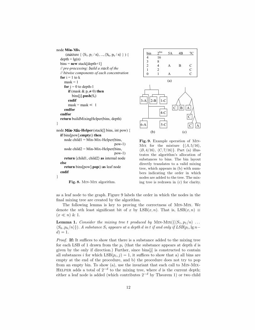
The idea behind the algorithm, which we refer to as Min-Mix, is to placea leaf node with sample 〈S〉 at depth d in the mixing tree if and only if thetarget concentration for S has a 1 in bit lg n − d of its binary representation.Theorem 1 then ensures that all substances have the desired concentrations,while fewer than lg n samples are used for each one.

Psuedocode for Min-Mix appears in Figure 8. We illustrate its operation forthe example mixture of {〈A, 5/16〉, 〈B, 4/16〉, 〈C, 7/16〉}. As shown in Figure 9,the algorithm begins with a pre-processing stage that allocates substances tobins according to the binary representation of the target concentrations. It thenbuilds the mixing tree via calls to Min-Mix-Helper, which descends throughthe bins. When a bin is empty, an internal node is created in the graph and theprocedure recurses into the next bin. When a bin has a substance identifier init, the substance is removed from the bin and a corresponding sample is added

3 lg n denotes log2n.

11

node �������������( � � ture { ⟨S1, p1 / n⟩, ..., ⟨Sk, pk / n⟩ } ) {

depth = lg(n)

bins = new stack[depth+1]

// pre-pr����� ssing: ����� ld a st����� of the

// bitwise components of each concentration

for i = 1 to k

mask = 1

for j = 0 to depth-1

if (mask & pi ≠ 0) then

bins[j].push(Si)

endif

mask = mask << 1

endfor

endfor

return buildMixingHelper(bins, depth)

}

node ��������������� Helper (stack[] bins, int pow) {

if bins[pow].empty() then

node child1 = Min-Mix-Helper(bins,

node child2 = Min-Mix-Helper(bins,

return ⟨child1, child2⟩ as internal node

else return bins[pow].pop() as leaf node

endif

}

pow-1)

pow-1)

Fig. 8. Min-Mix algorithm.

bin 2bin

5A 4B 7C

4 16

3 8

2 4 A B C

1 2 C

0 1 A C

C

C B A

C A

4-C

3-A 2-B 1-C

5-C 6-A

(a)

(b) (c)

Fig. 9. Example operation of Min-

Mix for the mixture {〈A, 5/16〉,〈B, 4/16〉, 〈C, 7/16〉}. Part (a) illus-trates the algorithm’s allocation ofsubstances to bins. The bin layoutdirectly translates to a valid mixingtree, which appears in (b) with num-bers indicating the order in whichnodes are added to the tree. The mix-ing tree is redrawn in (c) for clarity.

as a leaf node to the graph. Figure 9 labels the order in which the nodes in thefinal mixing tree are created by the algorithm.

The following lemma is key to proving the correctness of Min-Mix. Wedenote the nth least significant bit of x by LSB(x, n). That is, LSB(x, n) ≡(x � n) & 1.

Lemma 1. Consider the mixing tree t produced by Min-Mix({〈S1, p1/n〉 . . .〈Sk, pk/n〉}). A substance Si appears at a depth d in t if and only if LSB(pi, lg n−d) = 1.

Proof. If: It suffices to show that there is a substance added to the mixing treefor each LSB of 1 drawn from the pi (that the substance appears at depth d isgiven by the only if direction.) Further, since bins[j] is constructed to containall substances i for which LSB(pi, j) = 1, it suffices to show that a) all bins areempty at the end of the procedure, and b) the procedure does not try to popfrom an empty bin. To show (a), use the invariant that each call to Min-Mix-

Helper adds a total of 2−d to the mixing tree, where d is the current depth;either a leaf node is added (which contributes 2−d by Theorem 1) or two child

12

nodes are added, contributing 2∗2−(d+1) = 2−d. But since the initial depth is 0,the external call results in 20 = 1 unit of mixture being generated. Since the binsrepresent exactly one unit of mixture (i.e.,

∑

j bins[j] ∗ 2−j = 1), all bins will beused. To show (b), observe that Min-Mix references the bins in order, testing ifeach is empty before proceeding. Thus no empty bin will ever be dereferenced.

Only if: When a substance is added to the tree from bins[j], it appearsat depth lg n − j in the tree. This is evident from the recursive call in Min-

Mix-Helper: it initially draws from bins[lg n] and then works down when theupper bins are empty. By construction, bins[j] contains only substances Si withLSB(pi, j) = 1. Thus, if Si appears at depth d in the mixing tree, it was addedfrom bins[lg n − d] which has LSB(pi, lg n − d) = 1. ut

The following theorem asserts the correctness of Min-Mix.

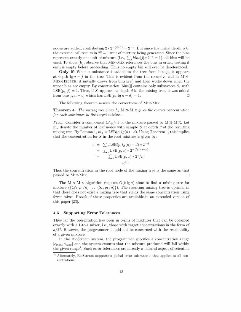
Theorem 4. The mixing tree given by Min-Mix gives the correct concentrationfor each substance in the target mixture.

Proof. Consider a component 〈S, p/n〉 of the mixture passed to Min-Mix. Letmd denote the number of leaf nodes with sample S at depth d of the resultingmixing tree. By Lemma 1, md = LSB(p, lg(n)−d). Using Theorem 1, this impliesthat the concentration for S in the root mixture is given by:

c =∑

d LSB(p, lg(n) − d) ∗ 2−d

=∑

x LSB(p, x) ∗ 2−(lg(n)−x)

=∑

x LSB(p, x) ∗ 2x/n

= p/n

Thus the concentration in the root node of the mixing tree is the same as thatpassed to Min-Mix. ut

The Min-Mix algorithm requires O(k lg n) time to find a mixing tree formixture ({〈S1, p1/n〉 . . . 〈Sk, pk/n〉}). The resulting mixing tree is optimal inthat there does not exist a mixing tree that yields the same concentration usingfewer mixes. Proofs of these properties are available in an extended version ofthis paper [23].

4.3 Supporting Error Tolerances

Thus far the presentation has been in terms of mixtures that can be obtainedexactly with a 1-to-1 mixer, i.e., those with target concentrations in the form ofk/2d. However, the programmer should not be concerned with the reachabilityof a given mixture.

In the BioStream system, the programmer specifies a concentration range[cmin, cmax] and the system ensures that the mixture produced will fall withinthe given range4. Such error tolerances are already a natural aspect of scientific

4 Alternately, BioStream supports a global error tolerance ε that applies to all con-centrations.

13

experiments, as all measuring equipment has a finite precision that is carefullynoted as part of the procedure. Given a concentration range, the system increasesthe internal precision d until some concentration k/2d (which can be obtainedexactly) falls within the range.

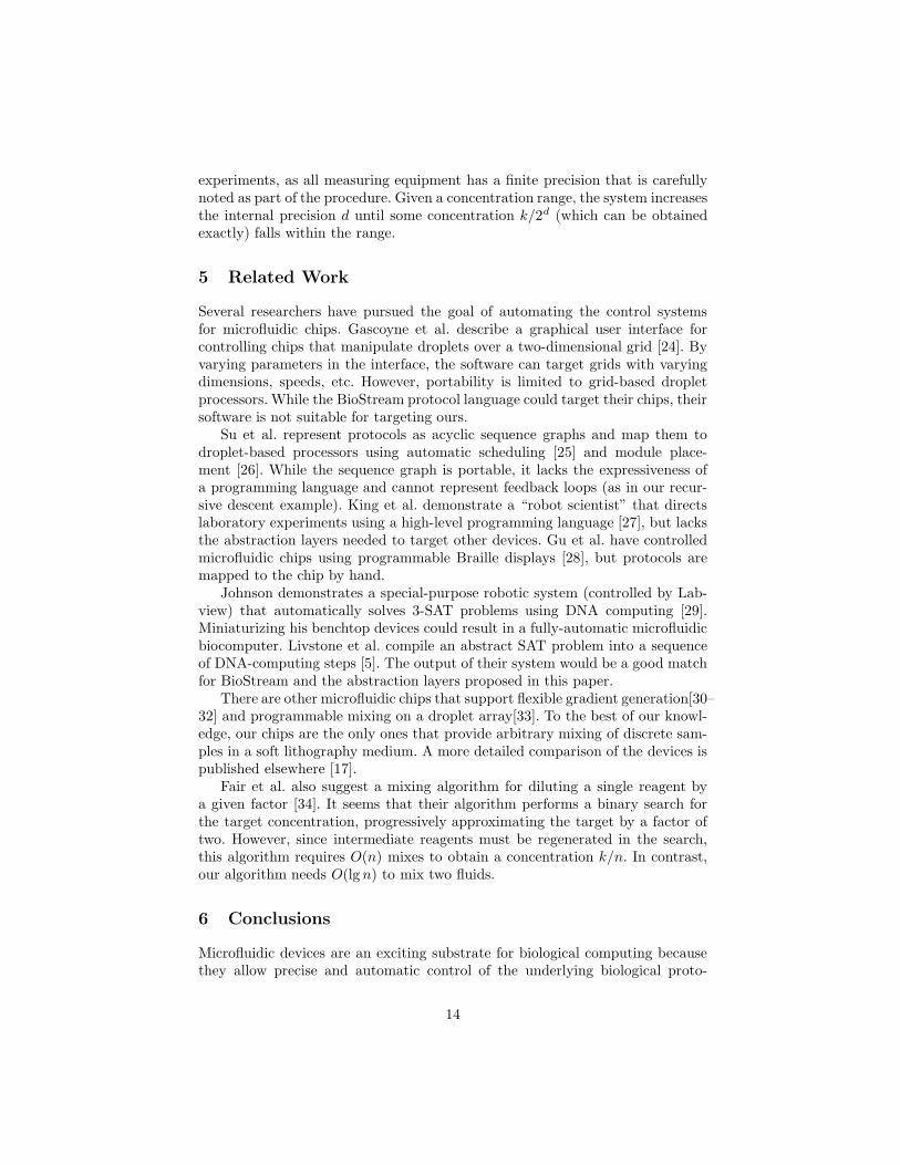
5 Related Work

Several researchers have pursued the goal of automating the control systemsfor microfluidic chips. Gascoyne et al. describe a graphical user interface forcontrolling chips that manipulate droplets over a two-dimensional grid [24]. Byvarying parameters in the interface, the software can target grids with varyingdimensions, speeds, etc. However, portability is limited to grid-based dropletprocessors. While the BioStream protocol language could target their chips, theirsoftware is not suitable for targeting ours.

Su et al. represent protocols as acyclic sequence graphs and map them todroplet-based processors using automatic scheduling [25] and module place-ment [26]. While the sequence graph is portable, it lacks the expressiveness ofa programming language and cannot represent feedback loops (as in our recur-sive descent example). King et al. demonstrate a “robot scientist” that directslaboratory experiments using a high-level programming language [27], but lacksthe abstraction layers needed to target other devices. Gu et al. have controlledmicrofluidic chips using programmable Braille displays [28], but protocols aremapped to the chip by hand.

Johnson demonstrates a special-purpose robotic system (controlled by Lab-view) that automatically solves 3-SAT problems using DNA computing [29].Miniaturizing his benchtop devices could result in a fully-automatic microfluidicbiocomputer. Livstone et al. compile an abstract SAT problem into a sequenceof DNA-computing steps [5]. The output of their system would be a good matchfor BioStream and the abstraction layers proposed in this paper.

There are other microfluidic chips that support flexible gradient generation[30–32] and programmable mixing on a droplet array[33]. To the best of our knowl-edge, our chips are the only ones that provide arbitrary mixing of discrete sam-ples in a soft lithography medium. A more detailed comparison of the devices ispublished elsewhere [17].

Fair et al. also suggest a mixing algorithm for diluting a single reagent bya given factor [34]. It seems that their algorithm performs a binary search forthe target concentration, progressively approximating the target by a factor oftwo. However, since intermediate reagents must be regenerated in the search,this algorithm requires O(n) mixes to obtain a concentration k/n. In contrast,our algorithm needs O(lg n) to mix two fluids.

6 Conclusions

Microfluidic devices are an exciting substrate for biological computing becausethey allow precise and automatic control of the underlying biological proto-

14

cols. However, as the complexity of microfluidic hardware comes to rival that ofsilicon-based computers, it will be critical to develop effective abstraction layersthat decouple application development from low-level hardware details.

This paper presents two new abstraction layers for microfluidic biocomputers:the BioStream protocol language and the Fluidic ISA. Protocols expressed inBioStream are portable across all devices implementing a given Fluidic ISA. Wedemonstrate this portability by building two fundamentally different microfluidicdevices that support execution of the same BioStream code. We also present anew and optimal algorithm for obtaining a given concentration of fluids using asimple on-chip mixing device. This algorithm is essential for efficiently supportingthe mix abstraction in the BioStream language.

It remains an interesting area of future work to leverage DNA computingtechnology to target the BioStream language from a high-level description of thecomputation. This will create an end-to-end platform for biological computingthat is seamlessly portable across future generations of microfluidic chips.

7 Acknowledgements

We are grateful to David Wentzlaff and Mats Cooper for early contributionsto this research. We also thank John Albeck for helpful discussions about ex-perimental protocols. This work was supported by National Science Foundationgrant #CCF-0541319. J.P.U. was funded in part by the National Science andEngineering Research Council of Canada (PGSM Scholarship).

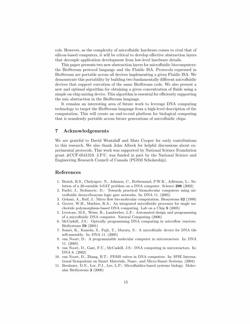
References

1. Braich, R.S., Chelyapov, N., Johnson, C., Rothemund, P.W.K., Adleman, L.: So-lution of a 20-variable 3-SAT problem on a DNA computer. Science 296 (2002)

2. Farfel, J., Stefanovic, D.: Towards practical biomolecular computers using mi-crofluidic deoxyribozyme logic gate networks. In: DNA 11. (2005)

3. Gehani, A., Reif, J.: Micro flow bio-molecular computation. Biosystems 52 (1999)4. Grover, W.H., Mathies, R.A.: An integrated microfluidic processor for single nu-

cleotide polymorphism-based DNA computing. Lab on a Chip 5 (2005)5. Livstone, M.S., Weiss, R., Landweber, L.F.: Automated design and programming

of a microfluidic DNA computer. Natural Computing (2006)6. McCaskill, J.S.: Optically programming DNA computing in microflow reactors.

BioSystems 59 (2001)7. Somei, K., Kaneda, S., Fujii, T., Murata, S.: A microfluidic device for DNA tile

self-assembly. In: DNA 11. (2005)8. van Noort, D.: A programmable molecular computer in microreactors. In: DNA

11. (2005)9. van Noort, D., Gast, F.U., McCaskill, J.S.: DNA computing in microreactors. In:

DNA 8. (2002)10. van Noort, D., Zhang, B.T.: PDMS valves in DNA computers. In: SPIE Interna-

tional Symposium on Smart Materials, Nano-, and Micro-Smart Systems. (2004)11. Breslauer, D.N., Lee, P.J., Lee, L.P.: Microfluidics-based systems biology. Molec-

ular BioSystems 2 (2006)

15

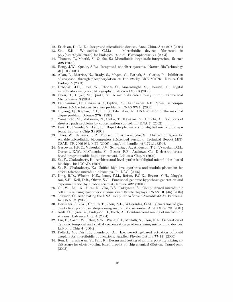
12. Erickson, D., Li, D.: Integrated microfluidic devices. Anal. Chim. Acta 507 (2004)13. Sia, S.K., Whitesides, G.M.: Microfluidic devices fabricated in

poly(dimethylsiloxane) for biological studies. Electrophoresis 24 (2003)14. Thorsen, T., Maerkl, S., Quake, S.: Microfluidic large scale integration. Science

298 (2002)15. Hong, J.W., Quake, S.R.: Integrated nanoliter systems. Nature BioTechnology

21(10) (2003)16. Allan, L., Morrice, N., Brady, S., Magee, G., Pathak, S., Clarke, P.: Inhibition

of caspase-9 through phosphorylation at Thr 125 by ERK MAPK. Nature CellBiology 5 (2003)

17. Urbanski, J.P., Thies, W., Rhodes, C., Amarasinghe, S., Thorsen, T.: Digitalmicrofluidics using soft lithography. Lab on a Chip 6 (2006)

18. Chou, H., Unger, M., Quake, S.: A microfabricated rotary pump. BiomedicalMicrodevices 3 (2001)

19. Faulhammer, D., Cukras, A.R., Lipton, R.J., Landweber, L.F.: Molecular compu-tation: RNA solutions to chess problems. PNAS 97(4) (2000)

20. Ouyang, Q., Kaplan, P.D., Liu, S., Libchaber, A.: DNA solution of the maximalclique problem. Science 278 (1997)

21. Yamamoto, M., Matsuura, N., Shiba, T., Kawazoe, Y., Ohuchi, A.: Solutions ofshortest path problems by concentration control. In: DNA 7. (2002)

22. Paik, P., Pamula, V., Fair, R.: Rapid droplet mixers for digitial microfluidic sys-tems. Lab on a Chip 3 (2003)

23. Thies, W., Urbanski, J.P., Thorsen, T., Amarasinghe, S.: Abstraction layers forscalable microfluidic biocomputers (Extended version). Technical Report MIT-CSAIL-TR-2006-034, MIT (2006) http://hdl.handle.net/1721.1/32543.

24. Gascoyne, P.R.C., Vykoukal, J.V., Schwartz, J.A., Anderson, T.J., Vykoukal, D.M.,Current, K.W., McConaghy, C., Becker, F.F., Andrews, C.: Dielectrophoresis-based programmable fluidic processors. Lab on a Chip 4 (2004)

25. Su, F., Chakrabarty, K.: Architectural-level synthesis of digital microfluidics-basedbiochips. In: ICCAD. (2004)

26. Su, F., Chakrabarty, K.: Unified high-level synthesis and module placement fordefect-tolerant microfluidic biochips. In: DAC. (2005)

27. King, R.D., Whelan, K.E., Jones, F.M., Reiser, P.G.K., Bryant, C.H., Muggle-ton, S.H., Kell, D.B., Oliver, S.G.: Functional genomic hypothesis generation andexperimentation by a robot scientist. Nature 427 (2004)

28. Gu, W., Zhu, X., Futai, N., Cho, B.S., Takayama, S.: Computerized microfluidiccell culture using elastomeric channels and Braille displays. PNAS 101(45) (2004)

29. Johnson, C.: Automating the DNA Computer to Solve n-Variable 3-SAT Problems.In: DNA 12. (2006)

30. Dertinger, S.K.W., Chiu, D.T., Jeon, N.L., Whitesides, G.M.: Generation of gra-dients having complex shapes using microfluidic networks. Anal. Chem. 73 (2001)

31. Neils, C., Tyree, Z., Finlayson, B., Folch, A.: Combinatorial mixing of microfluidicstreams. Lab on a Chip 4 (2004)

32. Lin, F., Saadi, W., Rhee, S.W., Wang, S.J., Mittalb, S., Jeon, N.L.: Generation ofdynamic temporal and spatial concentration gradients using microfluidic devices.Lab on a Chip 4 (2004)

33. Pollack, M., Fair, R., Shenderov, A.: Electrowetting-based actuation of liquiddroplets for microfluidic applications. Applied Physics Letters 77(11) (2000)

34. Ren, H., Srinivasan, V., Fair, R.: Design and testing of an interpolating mixing ar-chitecture for electrowetting-based droplet-on-chip chemical dilution. Transducers(2003)

16