WCAE 2009 Workshop on Computer Architecture Education

WCAE 2009

Proceedings of the

Workshop on Computer Architecture Education

in conjunction with

The 42nd International Symposium on Microarchitecture

Westin New York at Times Square New York City

December 13, 2009

Workshop on Computer Architecture Education Sunday, December 13, 2009

Program Chair: Michael Manzke, Trinity College, Dublin

General Chair: Ed Gehringer, North Carolina State U.

Program Committee: João Cardoso, FEUP/University of Porto, Portugal Dan Connors, University of Colorado James Conrad, University of North Carolina at

Charlotte Daniel Ernst, University of Wisconsin, Eau Claire Richard Enbody, Michigan State University Mark Fienup, University of Northern Iowa Diana Franklin, University of California, Santa

Barbara Subramanian Ganesan, Oakland University Ed Gehringer, NC State Zhiming Gu, Beijing Institute of Technology

David Kaeli, Northeastern University Nirav Kapadia, Unisys Corporation Jörg Keller, Fernuniversität Hagen Xiang Long, Beihang University Michael Manzke, Trinity College, Dublin Aleksandr Milenkovic, University of Alabama at

Huntsville Yale Patt, University of Texas at Austin Antonio Prete, Università di Pisa Mitch Thornton, Southern Methodist University Manish Vachhajarani, University of Colorado Anujan Varma, University of California at Santa

Cruz Chris Vickery, City University of New York Wang Dongsheng, Tsinghua University Xue Wei, Tsinghua University Craig Zilles, University of Illinois

Paper Session 1. 1:30–2:45

“Processor energy and temperature in computer architecture courses: a hands-on approach,” Sergio Gutierrez-Verde, , Octavio Benedi-Sanchez, Dario Suarez-Gracia, Jose Maria Marin-Herrero, and Victor Vinals-Yufera, Universidad de Zaragoza ........................................................................................... 1

“Examples from integrating systems research into undergraduate curriculum,” John H. Kelm, Steven S. Lumetta, University of Illinois......................................................................................................................... 9

“Circuit modeling in DLSim 3,” Richard M. Salter, John L. Donaldson, Serguei Egorov, and Kiron Roy, Oberlin College........................................................................................................................................ 17

Demo Session 1. 2:45–3:00

The MARS simulator for MIPS assembly in CS education, Pete Sanderson, Otterbein College

Break 3:00–3:30

Session 2. 3:30–4:15

“A two-tiered modeling framework for undergraduate computer architecture courses,” Jason Loew and Dmitry Ponomarev, State University of New York at Binghamton ............................................................. 24

“SimMips A MIPS system simulator,” Naoki Fujieda, Tokyo Institute of Technology, and Takefumi Miyoshi and Kenji Kise, Tokyo Institute of Technology and Japan Science and Technology Agency .... 32

Panel. 4:15–5:15

“Teaching multi-core architectures and compilers, from general purpose machines to GPUs”, Sam Midkiff, University of Illinois; Bruce Shriver, Genesis 2, Inc.; Tor M. Aamodt, University of British Columbia

Conclusion and Discussion. 5:15–5:30

Processor Energy and Temperature in Computer Architecture Courses: ahands-on approach

Sergio Gutierrez-Verde Octavio Benedı-SanchezDarıo Suarez-Gracia Jose Marıa Marın-Herrero† Vıctor Vinals-Yufera

gaZ. Dpto. de Informatica e Ingenierıa de Sistemas† Gitse. Dpto. de Ingenierıa Mecanica

I3A–Universidad de ZaragozaC\Marıa de Luna 1. E-50018 Zaragoza, Spainhttp://webdiis.unizar.es/gaz/

Abstract

Performance has driven the microprocessor industry formore than thirty years. Its effort has enabled to multiply byseveral orders of magnitude the computational power; e.g.,the Intel 8080 was able to execute 0.64 MIPS and the newestCore i7 can execute 6400 MIPS. The cost of this fabulousimprovement has been a large rise in energy consumption.Nowadays, we have reached a point where one of the mostlimiting factor for improving performance is energy dissi-pation.

In order to keep the performance improvement duringthe next years, it is necessary to study energy and tempera-ture in deep. Nevertheless, most current computer architec-ture curricula include neither energy nor temperature.

The lack of adequate experimental platforms contributesto the difficulty in teaching these topics. In this paper wepropose a possible solution: to instrument a commodity PCfor measuring the processor power and temperature duringthe execution of real programs. The platform is devised forteaching, but it can be used to support research experimentsas well. For example, we describe an interesting under-graduate laboratory that analyzes the interaction betweencompiler optimizations and energy. With this laboratory,students can learn that performance optimizations usuallyreduce energy but may increase power.

1 Introduction

Recently, designing energy-efficient computers or reduc-ing energy consumption is going beyond marketing strate-gies or personal experiences to turn into a collective goal forgovernments, societies, or companies. For instance, GreenComputing advocates for an environmentally sustainable

computing and communication, with minimal or no impacton the environment. Together with the concepts of total costof ownership, including the cost of disposal and recycling,the economics of energy efficiency is a key point of GreenComputing. So we think that computer engineers should beaware of these issues.

Energy-efficient computers are not only important froma Green Computing perspective, but also from a pure per-formance point of view. On one hand, in the embeddeddomain, lowering the energy consumed by the processor in-crements the device uptime. On the other hand, in the com-modity segment, the cooling system affects performancewhen it is not able to dissipate all the generated heat andforces a processor frequency/voltage reduction.

While the study of many design constrains, such as per-formance or programmability, may be done by means ofwhite boards or simulators, evaluation of energy and tem-perature appeals for hands-on laboratories—where studentsdeal with real—for many reasons such as: 1) This approachreinforces their physics background and establish a clearconnection between computer architecture and its imple-mentation; 2) They will quickly learn the importance of en-ergy dissipation and temperature by watching for examplehow fast a processor shutdowns when its fan stops; 3) En-ergy and temperature simulations require sophisticated en-vironments for being accurate, and since energy depends onboth the instructions and their data, the simulation time canbe very high and unfordable in two/three hour lab sessions.

The main barrier this hands-on approach faces is thelack of well established platforms for carry on the mea-surements. Many authors have performed processor powermeasurements either research oriented such Isci et al. oracademic oriented like Asın et al. [3]. Others such us Mesa-Martınez et al. have measured temperature in commodityPCs [17]. But up to our knowledge there is not an ade-

Page 1 Workshop on Computer Architecture Education (WCAE '09) December 13, 2009

quate platform able to simultaneously measure both magni-tudes. The present work extends the Asın et al. platformadding temperature monitoring support and automatic syn-chronization of the sampling process. The resulting plat-form improves measurement accuracy and data logging ca-pabilities, and at the same time its academic capabilitiessuch ease of use or cost are reinforced.

Platform features are presented by means of a labora-tory intended use case for last year undergraduate or mas-ter courses. Our final goal is to use this platform with stu-dents from both Computer Engineering (Computer Archi-tecture courses) and Mechanical Engineering (Heat Trans-fer courses) degrees in our institution to make them work-ing together in a common problem. As a session suitablefor both kind of students we present a lab dealing with theinteraction between compiler optimizations and energy.

Summarizing, the contributions of this work are the fol-lowing: we improve an existing platform for measuring en-ergy and temperature in commercial processors extendingits logging capabilities and improving the sampling accu-racy. We present the potential of the platform with a inter-esting laboratory in which the relation of power and tem-perature and the impact of compiler optimization in energyand power are analyzed.

This paper is organized as follows. Section 2 commentson the related work. Section 3 describes the measurementplatform in detail. Section 4 explains some test for validat-ing the platform. Section 5 describes the example labora-tory. Section 6 concludes and present some possible futurework lines.

2 Related Work

Energy and temperature have aroused the interest in bothindustry and academia. In the industrial side, SPEC has in-troduced SPECpower ssj2008 focusing on server computerconsumption [6], and EEMBC has defined EnergyBench es-tablishing a framework for adding energy to the metrics ofthe EEMBC’s performance benchmarks [5].

Many studies have been conducted in the academic side.Regarding energy, Isci and Martonosi describes a metho-dology for obtaining per-unit power estimations combiningreal power measurements with performance counters [14].Other authors have proposed infrastructures based on an In-tel Pentium 4 for characterizing program phases, evaluatingcompiler optimizations, or studying energy [9, 21, 3].

Temperature measurements have been performed withmore sophisticated setups; e.g., Mesa-Martınez et al. havepresented some power and temperature estimations using anexpensive IR thermal imaging equipment [16].

While most previous work focuses on energy and tem-perature from a research perspective, our work also takes

into consideration academia requirements such as simplic-ity or affordable cost.

3 Platform description

The measurement platform is based in our previous workand consists of two commodity PCs [3]. One, named com-puter under test (CUT), is monitored, and another, nameddata acquisition and storage computer (DASC), acquiresand saves all the power and temperature samples gatheredfrom the CUT. Both computers are shown in Figure 1a, theCUT in the left and the DASC in the right.

The CUT runs a GNU/Linux system with a 2.6.25 ker-nel in which all non-required modules and services (X-Windows, printing, USB, ...) have been removed to min-imize the energy consumed by the operating system tasks.The processor and the motherboard are a 2.8 Ghz Intel Pen-tium 4 Northwood and an ASUS P4 P8000, respectively.This motherboard employs a dedicated power line betweenthe power supply and the processor voltage regulator man-ager; thus, it removes the need of hacking the motherboardand simplifies the monitoring of the processor consump-tion because the product of the voltage of the VRM powerline times its current is the power drawn by the processor—assuming negligible the VRM consumption [2]. The abovedescribed power line is present on most current PCs, so thistechnique can be used with other hardware configurations.

The current is measured with a Tektronix TPC-312clamp ammeter [23]. The output of the clamp ammeteralong with the voltage are logged with an Adlink PCI-9112 [10] data acquisition card sampling at 2 Kilosam-ples/second per channel, 1000×more than the previous ver-sion of the platform. At this sampling rate, we are ableto observe the main program execution phases, and powertraces remain in reasonable sizes, lower than 1 GiByte.All samples are stored in the DASC in order to allow off-line analysis . The DASC system also runs GNU/Linuxand the previous LabView software has been replaced byC based code and some perl scripts because they allowedmuch higher sampling rates and we observed that the real-time visualization of LabView was seldom used. In fact,real-time visualization is useful for debugging the platform,but for that purpose an oscilloscope is preferable. The useof the new programs is straightforward with a small learn-ing time as it was with the LabView based software.

Current processors require large heat sinks with power-ful fans for cooling. Cold air flows towards the processorpushed by the fan and gets warmer. The hot air is expelledthrough the sides of the head sink as shown in Figure 1b.Since the air (a fluid) flows through a solid (each of the nar-row channels in between the parallel fins), the whole pro-cessor cooling package could be modeled according to aforced-convection thermal model. If some conditions are


Powersupply CPUVRM

Motherboard

12 v 1.6 v

Clamp ammeter

data adquisition andstorage computer (DASC)

.

computer under test (CUT)

.

Cooling system

thermo-couples

ethernet

(a) Component diagram.

1

6

5

2

3 4

(b) Thermocouple localization in the processor–cooling package. . Thecold air, pushed by the fan, flows through the narrow channels in betweenthe fins : it enters top-down and exits horizontally, either by the left and theright sides

Figure 1: Overview of the platform with its main components

meet, and forced convection holds, heat transfer, q, becomesproportional to dissipation area, A, and gradient tempera-ture, ∆T :

q = h×A×∆T

Being the constant h an (experimental) number dependingmainly on thermal conductivity, speed of the flow, and chan-nel geometry [11]. Acquiring temperature at multiple pointswill help us to determine the model goodness. Measure-ments are carried with K-type thermocouples optimized forthe temperature range of 0-100 °C that are located at 6 po-sitions: 1) drilled in middle of the heat sink contacting withthe processor, 2) drilled in the border of the heat sink—Intel provides some guidelines for the placement at theselocations [13], 3) in the lateral edge of a fink placed in themiddle of the heat sink, 4) in the lateral edge of a fink placedin a corner of the heat sink, 5) in the free path of the outputhot air flow without touching the heat sink, and 6) in thefree path of the input cold air flow.

The six measurement points ease the verification of theforced convection model because from this model we knowthat the temperature of the hot air flow should be muchbigger than that of the cold air flow. Also, the temper-ature should rise as we approach close to the processor;therefore, in the real measures we have to observe thatTemp(5) >> Temp(6) and Temp(T1) > Temp(T2).

The acquisition of temperature samples is done with a Pi-cotech TC-08 converter that is connected to a USB port ofthe DASC [22]. The conversion frequency depends on thenumber of attached thermocouples. In our case, 6 thermo-couples, the data acquisition rate is 0.73 samples/second, sothat any individual thermocouple gets sampled every 4,4 s.This rate is much smaller than that of power, but it is enoughbecause the change rate of temperature is much lower thanthat of power as we will see in Section 4.

Since the platform uses two computers, it is required tosynchronize the beginning and the end of the sampling pro-

cess. The synchronization is acomplished by sending twolow-latency Ethernet packets, one just at the beginning ofthe execution of the program under test and the other justafter its end. This synchronization schema is done by awrapper on the executables that avoids any complexity tothe students, even for those without a good shell knowledge.The platform is able to monitor any program independentlyof its execution time as long as the hard disk drive has spaceleft.

Summarizing, the platform is able to measure the tem-perature and the energy drawn by the execution of any pro-gram in an Intel Pentium 4 processor with high precisionand without interfering the computer under test. All theplatform software is freely available upon request.

4. Platform Validation

Most changes in the hardware of the platform with re-gards to the previous version were motivated for increasingthe sampling accuracy and for logging power and temper-ature simultaneously. The objective was to detect powerphases during program execution, and to see how changesin energy consumption affected temperature.

As a prove of the accuracy of the platform, Figure 2shows the temporal evolution of power and temperature forthe complete run of 473.astar (SPEC CFP2006) com-piled at the maximum level of optimizations with Intel Ccompiler1.

The left Figure, 2a, shows the instant power and temper-ature at the center of the heat sink (thermocouple 1 in Fig-ure 1b). Note that with this easy experiment students cansee how changes in the phases of programs also affects toits energy consumption, and how temperature reacts slowlyto the changes in power—justifying the choice of a muchlower sample rate for temperature than for power. Besides,

1For more methodology details please read Section 5.


this plot also shows how the processor–heatsink–fan sys-tem tends towards their thermodynamic equilibrium whenpower is almost constant after roughly 130 s (this can be no-ticed in both the 150-300 and 600-800 time windows). Oursoftware package includes a PID controller able to stabilizethe processor consumption, or alternatively the temperature,at a given value for performing these kind of experiments ina controlled way.

In order to employ the forced convection model of theprocessor—cooling package we have to take several steps.The first one is to verify relations among the measured tem-peratures. As shown in the right Figure, 2b, the output airtemperature (T5) is warmer that the input one (T6), and thedifference in temperature increases as the processor activityrises. Once the initiation phase is completed, the temper-ature difference between the processor– headsink packageand the input air (T2 - T6) is large (a maximum of almost30 °C) while the difference between the processor-headsinkpackage and the output air (T2 - T5) is small (less than 5°C). These differences between both values indicate that theair is absorbing heat from the headsink and spreads it out ofthe processor–headsink package. Also the temperature inthe middle of the heat sink (T1) is bigger than that of theborder of the heat sink (T2). All these relations match withthe model expectations.

The second step involves considering also the fin tem-peratures (T3 and T4), determine which gradient tempera-ture has to be computed (∆T ), and tune the experimentalconstant h. We have some preliminary numbers, allowingus to approximate the package temperature from the powerdrawn by the processor, but we do not show the numbersbecause the model is not accurate enought; the h constantdoes not completely match with the handbook data nor-mally used in thermal engineering.

5 Example Laboratory

This section describes a laboratory to get some insightsbetween compiler optimizations and energy/power and thencomments some other challenging experiments using thethermal measurement abilities of the platform.

5.1 Interaction between Compiler Opti-mization and Energy/Power

One possible application of the platform in academia isits use in computer architecture laboratories. For example,it easily allows to study the interaction between compileroptimizations and energy/power.

The lab would be introduced by explaining the basic re-lationships among time, energy, and power paying attentionto what changes should be expected when the optimizationlevel rises. An outline of such introduction follows.

In a processor without Dynamic Voltage Frequency Scal-ing (DVFS), the execution time Tex of a program can beexpressed as

Tex = Ninst × CPI × Tcycle (1)

where Ninst, CPI , and Tcycle represents the total num-ber of instructions, the average number of cycles per in-struction, and the cycle time, respectively. For minimizingTex, compilers focus on reducing the total number of cycles,Ninst × CPI . But which are the effects of this reductionon power and energy?

Assuming the simplifying assumption that static biascurrent does not flow in a microprocessor [20], its totalpower consumption is given by

Ptot = Pdyn + Psta = CLV 2ddf + VddIleak (2)

where Ptot is the total sum of the dynamic and static power.The dynamic power, Pdyn, is the product of the average ca-pacitance switched per cycle (processor activity), CL, timesthe square of the supply voltage, Vdd, times the frequency,f . The static power is the product of the supply voltagetimes leakage current, Ileak [19].

From equations (1) and (2) we observe that compileroptimizations only affect power indirectly. Regarding dy-namic power, Pdyn, on one hand, it is difficult to estab-lish a relationship between Ninst and CL because execut-ing more, less, or different instructions may or may notchange the performed activity per cycle. On the other hand,CPI seems to impact more the dynamic power (CL) be-cause optimizations that rise/reduce Instruction Level Par-allelism (ILP), such as instruction scheduling or dead-codeelimination, can increase/decrease activity per cycle, CL.

Static power is less affected by compiler optimizationssince it depends mostly on technological parameters; how-ever, they can affect static power when the optimizationsincrease/decrease the processor activity and this results ina variation of processor temperature because leakage cur-rent depends on temperature [4]. The most straightforwardpath for reducing static power from compilation is to addspecial instructions in the code for switching off processorparts as suggested by Zhang et al. [26]. These proposalswill become more and more important in the future becauseas technology scales, the percentage of static power is ris-ing [15].

The product of Ptot times Tex is the energy consumedby a program

Etot = Ptot × Tex = Edyn + Esta

= CtotV2dd + VddIleak × Tex (3)

where Ctot is the total capacitance that has been switchedacross all execution cycles.


40

45

50

55

60

65

0 100 200 300 400 500 600 700 800 900 35

43

51

59

67

75

Pow

er (W

)

Tem

pera

ture

(o C)

Time (s)

Power Temperature

(a) Temperature in thermocouple 1 and Power

25

35

45

55

65

75

0 100 200 300 400 500 600 700 800 900

Tem

pera

ture

(o C)

Time (s)

∆T Air

∆T Air

T1

T6

T5T2

center heat sink T1border heat sink T2

output air T5input air T6

(b) Temperature at thermocouples

Figure 2: Temperature and Power temporal evolution during the full execution of 473.astar compiled with iO3prf options.

Recalling equations (1) and (3), Edyn is independent ofthe frequency and

Ctot = CL ×Ninst × CPI (4)

Thus, execution-time optimization saves energy whenthey reduce the total number of cycles, Ninst × CPI , be-cause we do not expect that compiler optimizations increasesignificantly CL. In deep-pipelined processors with com-plex decoding such as the Intel Pentium 4, this is speciallytrue because the energy consumed in the execution stage issmaller that the energy consumed in the rest.

Table 1: Compiler optimization impact summary. ↓, ?, and↑ means decrement, undetermined, and increment, respec-tively.

Power Ninst ↓ CPI ↓dynamic (Pdyn) ? ↑static (Psta) ? ?

Energy Ninst ↓ CPI ↓dynamic (Edyn) ↓ ↓static (Esta) ↓ ?

Table 1 summarizes all previous relations and de-rives the effect of decreasing either Ninst or CPI , as-suming constant the other factor. As it can be seen,performance-oriented compiler optimizations (focused onreducing Ninst × CPI) are beneficial for energy, and maynot be power-efficient when their target is to reduce onlythe CPI because dynamic power can increase. Asking thestudents to complete this table before the laboratory sessionis a good assignment for ensuring that students understandthe underneath theory.

5.1.1 Experimental Results

0.4

0.5

0.6

0.7

0.8

0.9

1

0.4 0.5 0.6 0.7 0.8 0.9 1

Ene

rgy

rela

tive

to g

O0

Execution Time relative to gO0

gO0

gO2

gO3

gO3prf

iO3prf

(a) Integer

0.4

0.5

0.6

0.7

0.8

0.9

1

0.4 0.5 0.6 0.7 0.8 0.9 1

Ene

rgy

rela

tive

to g

O0

Execution Time relative to gO0

gO0

gO2

gO3

gO3prf

iO3prf

(b) Floating Point

Figure 3: Average Energy and Execution time relative togO0.


Table 2: Tested SPEC CPU2006 benchmarks.

Integer Input Floating Point Input400.perlbench -I./lib checkspam.pl 2500 5 25

11 150 1 1 1 1436.cactusADM benchADM.par

462.libquantum 1397 8 437.leslie3d -i leslie3d.in473.astar rivers.cfg 447.dealII 23483.xalancbmk -v t5.xml xalanc.xsl 453.povray SPEC-benchmark-ref.ini

454.calculix -i hyperviscoplastic470.lbm 3000 reference.dat 0 0

100 100 130 ldc.of

Table 3: Compiler configurations with their respective optimization flags

Compiler FlagsgO0 gcc -O0gO2 gcc -O2 -mtune=pentium4 -march=pentium4gO3 gcc -O3 -mtune=pentium4 -march=pentium4 -mfpmath=sse,387 -msse2gO3prf gcc -O3 -mtune=pentium4 -march=pentium4 -mfpmath=sse,387 -msse2 -fprofile-generate/useiO3prf icc -O3 -xN -ipo -no-prec-div -prof-gen/use

The previous relations can be verified with the pro-posed platform by executing multiple programs with dif-ferent compiler optimizations and acquiring the energy andpower measurements. For the sake of brevity, we only showthe results for the relation between energy and executiontime.

As a benchmark we can choose any program not spend-ing most of the time in I/O to ensure that the impact ofcompiler optimization is significant in energy and power.Due to its widespread use in industry and academia SPECCPU2006 has been our choice [8]. In order to reduce themeasurement time we select the representative subset pro-posed by Phansalkar et al. [18]. The input sets for eachprogram used in this paper are shown in Table 2. Otherevents of interest such as fetch stalls or instruction count canbe measured with Intel Performance Tuning Utility (PTU);e.g., to compute the energy per instruction value [1].

To check the impact of compiler optimizations in en-ergy and power we suggest to test multiple configurationsof the GNU C compiler 4.1.2 (gcc) [7] and one config-uration of the Intel C compiler 10.1 (icc) [12], all listedin Table 3. As a baseline, we use a configuration withoutoptimizations, gO0. We also checked a production-levelconfiguration tuned for our processor, gO2. Finally, we en-courage using more aggressive gcc configurations: -O3without and with profiling, and icc at its maximum levelof optimizations with profiling (iO3prf).

In integer, the more optimizations are applied, the betterthe results are. The best gcc configuration, gO3prf saves34.7% of execution time and 38% of energy. IO3prf in-creases the gains saving 46% and 48.4% of execution timeand energy, respectively. In floating point, optimizationsare more effective; i.e., gO2 (the best gcc configuration)saves 41.3% and 45.6% of execution time and energy, re-spectively. Again, iO3prf performs better with 59.6%and 62.8% reductions in execution time and energy.

Gains in execution time and energy are very close sug-gesting a strong correlation. To support this claim, Figure 4plots execution time and energy for each benchmark. Ascan be seen the correlation is strong, which is in line withprevious work [24, 21]. We believe that the correlation isdue to the fact that the clock net, static consumption, andfetch, decoding, and control parts of the processor consumemore than functional units [25]; hence, it seems than reduc-ing the number of executed instructions is more importantthan its kind for improving energy consumption.

Regarding execution time, icc beats gcc in all but onebenchmark, 447.dealII. Besides, icc consumes lessenergy in all programs but 470.lbm. To conclude, bothgcc and icc reduce notably the number of executed in-structions (50% and 75% on average for integer and float-ing point, respectively) and increase the CPI (rising also theEnergy per instruction) but icc does it in a lower quantity.

Summarizing, the main assignments for this lab can be:to perform the measurements for the program, to verify thatthe table they have completed before the lab is correct, andto finish extracting the conclusions of the previous para-graphs.

5.2 Other Experiments

The platform can be used with a more research-orientedfocus such as master dissertations. For example, an out-going work in our lab wants to obtain a power/temperatureprofile of individual instructions.

Since the processors’ manual does not document theconsumption of the instructions, we can get an estimationwith the platform . For example, we have observed thatstack operations rise power consumption and heat more theprocessor, which makes sense because stack instructions re-quire a read/write in the cache and one increment/decrementin the stack pointer register in the same cycle.


0

500

1000

1500

2000

2500

3000

3500

4000

gO0gO2

gO3gO3prf

iO3prf

gO0gO2

gO3gO3prf

iO3prf

gO0gO2

gO3gO3prf

iO3prf

gO0gO2

gO3gO3prf

iO3prf

20

45

70

95

120

145

170

195

220

Exe

cutio

n T

ime

(Sec

onds

)

Ene

rgy

(Kilo

Joul

es)

Execution Time Energy

483.xalancbmk473.astar462.libquantum400.perlbench

(a) Integer

0

1000

2000

3000

4000

5000

6000

7000

8000

gO0gO2

gO3gO3prf

iO3prf

gO0gO2

gO3gO3prf

iO3prf

gO0gO2

gO3gO3prf

iO3prf

gO0gO2

gO3gO3prf

iO3prf

gO0gO2

gO3gO3prf

iO3prf

gO0gO2

gO3gO3prf

iO3prf

0

62.5

125

187.5

250

312.5

375

437.5

500

Exe

cutio

n T

ime

(Sec

onds

)

Ene

rgy

(Kilo

Joul

es)

Execution Time Energy

470.lbm454.calculix453.povray447.dealII437.leslie3d436.cactusADM

(b) Floating Point

Figure 4: Execution time and Energy per benchmark.

6. Conclusions and Future Work

This paper presents a platform for measuring en-ergy/power and temperature in commodity PCs with an aca-demic focus. In this work, measures are carried out in anIntel Pentium 4, but the platform can be easily ported toany commodity PCs. The acquired data can be stored toperform off-line analysis, and its accuracy enables to detectpower and temperature phases.

With the platform students can, for example, studythe interaction between compiler optimizations and en-ergy/power. This laboratory enables the student to learn thaton average performance optimizations are energy-efficient.

Nowadays,the platform is used and extended by a smallgroup of students. Our next main step is to set up a wholelaboratory for using it as a regular laboratory session in ourComputer Architecture and Heat Transfer courses. Our on-going work is to obtain a simple linear equation relatingmeasured power, fan speed, and dissipating surface to com-pute output air temperature for using it during the introduc-tion of the laboratories.

Our future work will try to extend the platform reduc-ing the granularity of the sampling process. Now, the plat-form does not know at which code fragment or functioneach sample belongs. We believe that this ability will helpus finding the most heat-producing instruction sequences tocontinue our studies on per instruction energy estimations.

Acknoledgements

The authors would like to thank the anonymous review-ers for their suggestions on this paper. Darıo Suarez Gra-cia and Vıctor Vinals Yufera were supported in part by theGobierno de Aragon grant gaZ: Grupo Consolidado de In-vestigacion, the Spanish Ministry of Education and Scienceunder contracts TIN2007- 66423, TIN2007-68023-C02-01,and Consolider CSD2007- 00050, and the European UnionNetwork of Excellence HiPEAC-2 (FP7/ICT 217068).

References

[1] Intel Performance Tuning Utility 3.1 Update 3. http://software.intel.com/en-us/articles/intel-performance-tuning-utility-31-update-3,2007 edition.

[2] Analog Devices. ADP3180, 6-Bit Programmable 2-, 3-, 4-Phase Synchronous Buck Controller. Analog Devices, 2003.

[3] A. Asın Perez, D. Suarez Gracia, and V. Vinals Yufera. Aproposal to introduce power and energy notions in computerarchitecture laboratories. In WCAE ’07: Proceedings of the2007 workshop on Computer architecture education, pages52–57, New York, NY, USA, 2007. ACM.

[4] D. Brooks, R. P. Dick, R. Josepth, and L. Shang. Power,thermal, and reliability modeling in nanometer-scale micro-processors. IEEE Micro, 27(3):49–62, May-June 2007.


[5] E. T. E. M. B. Consortium. EnergyBench ™ version 1.0power/energy benchmarks. http://www.eembc.org/benchmark/power_sl.php, 2008.

[6] S. P. E. Corporation. SPECpower ssj2008 benchmark suite.http://www.spec.org/power_ssj2008/, 2008.

[7] Gcc team. GCC 4.1.2 Manual. http://gcc.gnu.org/onlinedocs/gcc-4.1.2/gcc/. Free Software Foun-dation, February 2008.

[8] J. L. Henning. Spec cpu2006 benchmark descriptions.SIGARCH Comput. Archit. News, 34(4):1–17, 2006.

[9] C. Hu, J. McCabe, D. A. Jimenez, and U. Kremer. Infre-quent basic block-based program phase classification andpower behavior characterization. In Proceedings of The 10th

IEEE Annual Workshop on Interaction between Compilersand Computer Architectures. ACM Press, 2006.

[10] A. T. Inc. Adlink pci-9112 data acquisition card.http://www.adlinktech.com/PD/web/PD_detail.php?cKind=&pid=29&seq=&id=&sid=,2008.

[11] F. P. Incropera, D. P. DeWitt, T. L. Bergman, and A. S.Lavine. Fundamentals of Heat and Mass Transfer. Wiley,6th edition, 2007.

[12] Intel. Intel C++ Compiler 10.1 Profesional edi-tion. http://www.intel.com/cd/software/products/asmo-na/eng/277618.htm, 2007edition.

[13] Intel. Intel® Pentium® 4 Processor in the 478-Pin PackageThermal Design Guidelines. Intel Corporation, 1st edition,May 2002.

[14] C. Isci and M. Martonosi. Runtime power monitoring inhigh-end processors: Methodology and empirical data. InMICRO 36: Proceedings of the 36th annual IEEE/ACMInternational Symposium on Microarchitecture, page 93,Washington, DC, USA, 2003. IEEE Computer Society.

[15] S. Kaxiras and M. Martonosi. Computer Architecture Tech-niques for Power-Efficiency. Number 4 in Synthesis Lec-tures on Computer Architecture. Morgan & Claypool Pub-lishers, 2008.

[16] F. J. Mesa-Martinez, M. Brown, J. Nayfach-Battilana, andJ. Renau. Measuring performance, power, and temperaturefrom real processors. In ExpCS ’07: Proceedings of the 2007workshop on Experimental computer science, page 16, NewYork, NY, USA, 2007. ACM.

[17] F. J. Mesa-Martinez, J. Nayfach-Battilana, and J. Renau.Power model validation through thermal measurements. InISCA ’07: Proceedings of the 34th annual internationalsymposium on Computer architecture, pages 302–311, NewYork, NY, USA, 2007. ACM.

[18] A. Phansalkar, A. Joshi, and L. K. John. Analysis of redun-dancy and application balance in the spec cpu2006 bench-mark suite. In ISCA ’07: Proceedings of the 34th annualinternational symposium on Computer architecture, pages412–423, New York, NY, USA, 2007. ACM.

[19] J. Rabaey. Low Power Design Essentials. Springer, 2009.[20] J. M. Rabaey, A. Chandrakasan, and B. Nikolic. Digital In-

tegrated Circuits. A design perspective. Prentice Hall Elec-tronics and VLSI series. Prentice Hall, second edition, 2003.

[21] J. S. Seng and D. M. Tullsen. The effect of compiler opti-mizations on pentium 4 power consumption. In Seventh An-nual Workshop on Interaction between Compilers and Com-puter Architectures (INTERACT’03, page 51, 2003.

[22] P. Technologies. USB TC-08 Temperature Logger User’sGuide. Pico Technologies Limited, 2007.

[23] Tektronix. Tektronix tpc-312 current probe.http://www2.tek.com/cmswpt/psdetails.lotr?ct=PS&ci=13540&cs=psu&lc=EN, 2008.

[24] M. Valluri and L. John. Is compiling for performance ==compiling for power? In Fifth Annual Workshop on Inter-action between Compilers and Computer Architectures (IN-TERACT’00), page 51, 2001.

[25] W. Wu, L. Jin, J. Yang, P. Liu, and S. X.-D. Tan. A system-atic method for functional unit power estimation in micro-processors. In DAC ’06: Proceedings of the 43rd annualconference on Design automation, pages 554–557, NewYork, NY, USA, 2006. ACM.

[26] W. Zhang, J. S. Hu, V. Degalahal, M. Kandemir, N. Vijaykr-ishnan, and M. J. Irwin. Compiler-directed instruction cacheleakage optimization. In Proceedings of the 35th AnnualIEEE/ACM International Symposium on Microarchitecture,page 208. IEEE Computer Society, 2002.


Examples from Integrating Systems Research into Undergraduate Curriculum

John H. Kelm and Steven S. LumettaUniversity of Illinois at Urbana-Champaign

{jkelm2, lumetta}@illinois.edu

Abstract

In this paper we motivate and discuss the use of examplesdrawn from computer systems research for use in the class-room. We describe three case studies used in an advancedundergraduate course covering large software system de-sign. The case studies document situations we have encoun-tered while designing and implementing performance mod-eling infrastructure and benchmark applications for use inour research on parallel processor design. Two of the casestudies cover debugging techniques and are available pub-licly. The third case study covers performance analysis us-ing freely available tools. The goals of this work are toillustrate how classroom concepts are realized in computersystems, to provide examples of how performance analysisand tuning can be applied to complex real-world applica-tions such as our C++ architectural simulator, to motivatethe use of profiling tools in instruction, and to expose stu-dents to research topics and methodology.

1 Introduction

This paper contains the summary and discussion of threecase studies that are intended for use in advanced under-graduate instruction. The case studies describe debuggingand optimization experiences from RigelSim, a C++ simu-lator for the Rigel architecture [11], and its correspondingruntime system. Two of the case studies involved remov-ing correctness bugs from RigelSim. The third case studydiscusses the application of performance analysis and opti-mization techniques to our simulator infrastructure. Thesecase studies were used in a senior undergraduate-level soft-ware systems class and serve as models that other instruc-tors could adopt. The goal of using case studies is to high-light the difficulty and subtlety involved in addressing cor-rectness and performance bugs in large systems that are oth-erwise difficult for students to see firsthand in class projects.

The first case study documents the experience of remov-ing a correctness bug in RigelSim that was hard to exposeand required long running simulations to activate. The casestudy highlights the need for innovative and methodical ap-proaches to debugging large computer systems. The casestudy discusses the need for regression testing and self-

checking mechanisms when working with evolving soft-ware systems that have multiple contributors. We discussthe utility of determinism and robustness in the debuggingprocess for large-scale applications. The goal of the study isto introduce students to one component of a large softwaresystem, describe a software error, and show them how onewould go about removing that error. Using an example fromour research allows us to provide a more in-depth perspec-tive and exposes students to the tools that researchers in thearea of computer architecture frequently use. An extendedversion of the case study is available online [9].

The second case study describes the process of isolat-ing and removing a livelock from the runtime system usedwithin RigelSim. The case study highlights three topicsrelevant to students. It describes the nature of a common,but difficult to diagnose condition in parallel systems. Sec-ondly, we motivate methodical and structured approachesto software system performance analysis. Lastly, the casestudy illustrates how latent performance bugs can remainundetected for long periods of time while sapping perfor-mance unbeknownst to the developers. A greater emphasisis being placed on developing parallel software. However,there is a lack of widespread experience with such systemsmaking case studies such as this a valuable resource forcomputer engineering students. An extended version of thecase study is available online [10].

The third case study discusses a number of experiencesusing sample-based profiling of our simulator tools to diag-nose performance pathologies in our code. We also discusshow students can benefit from these experiences and howother instructors could develop similar examples. We applywidely deployed and freely available tools to our simulatorinfrastructure, and in doing so, bring computer architectureresources into the classroom while providing students withtools they can apply more broadly.

The rest of the paper is as follows: Section 2 providesan overview of the course where these materials were firstused. Section 3 summarizes the debugging case studies.Section 4 discusses the performance analysis experiences.Section 5 provides discussion of the use of research experi-ences in the classroom. Section 6 concludes the paper.


Target Memory(Rigel Benchmark)

Host Memory(RigelSim/x86 Heap)

… …

Benchmark Code (.text segment)

Rigel Heap Rigel Stacks

Allocation from within RigelSim using new to return host address

Target Address: 0x40001bc4

Other RigelSim Data

Figure 1. Target-to-host memory mapping for RigelSim.

2 Course and Research Overview

The materials presented in this paper were used in anelective course offered in Spring 2009 at the University ofIllinois. The course focused on large software system de-sign. The course targeted advanced undergraduates andgraduate students. Professor Steven S. Lumetta designedand instructed the course.

The goal of the course was to provide students with anunderstanding of the relationship between application soft-ware, compilers, runtimes, and computer architecture. Thefirst half of the course focused on abstraction used in mod-ern programming languages. The course used C++ as an ex-ample language and used Stroustrup [17] as a text. The sec-ond half of the course covered parallel runtimes, commonparallel idioms, and the interplay between parallel softwaredevelopment and parallel architectures. Interwoven with thetwo major thrusts of the class were perspectives on debug-ging and performance analysis—the two topics consideredin this paper.

Additional materials, including lecture notes, laboratoryassignments, and supplemental material, are available onthe course website [14].

3 Correctness Case Studies

In this section we provide an overview of two case stud-ies used in the class. The first study discusses the isolationand removal of a software error from an architectural simu-lator used in our research. The second study concerns a live-lock condition found in the simulated parallel runtime forour design. Both case studies are available online [9, 10].

3.1 Memory Model Bug

Motivation The motivation for this case study is to givestudents a perspective on debugging large-scale softwaresystems. Developing tools and techniques to remove soft-ware errors from large systems requires ingenuity and ex-perience. Many students learn the technique of debugging

Target Memory(Rigel Benchmark)

Host Memory(RigelSim/x86 Heap)

… …

Two target addresses aliasing to the same host address

Target Address 1: 0x40001bc4 Target Address 2: 0x80001bc4

Figure 3. Target-to-host aliasing that caused the observedtarget memory corruption.

from class projects. Bottom-up approaches to introductorycomputer systems instruction [4, 15] exposes students to thedesign and implementation of computer systems. However,class projects rarely exceed a semester in length, thus lim-iting the size of the system with which students interact.Furthermore, when a large software system is used, suchas the Linux kernel, debugging tools and vetted infrastruc-ture already exists to aid in the isolation of software errors.The existence of debugging infrastructure and methodolo-gies lessens the need for holistic and innovative approachesto debugging, thus leaving students ill prepared for debug-ging large computer systems that lack widely accepted toolsand practices.

To help bridge the gap between the classroom and realworld large system design, we use case studies based onour own experience developing the simulation infrastruc-ture for the Rigel architecture. Using software errors foundin the development of our research infrastructure as exam-ples, we demonstrate how bugs can cross abstraction levelboundaries from the application down to the microarchitec-ture and how to isolate bugs in such an environment.

Description and Debugging Process Throughout thispaper, host refers to the x86 workstations that execute in-stances of RigelSim, while target refers to the simulatedRigel system. The case study concerns a bug in RigelSimthat caused two addresses in the target address space to mapto the same host address causing intermittent pointer cor-ruption. The component responsible for the error was thememory model for the simulator.

The bug discussed in the case study was found duringa nightly batch run of simulations. Of the 200+ jobs thatwere run, only four failed. Furthermore, the four failuresoccurred only after many hours of simulation. Due to thelong time to activation, we were constrained by the rate atwhich we could make a change to the system and observewhether the bug was corrected. The case study discusses theuse of information gathering techniques and testing philos-ophy that were employed to keep the test process tractable.


BYTE COL CONTROLLER BANK CHIP ROW

Ctrls[]

00 31

Target Address Bits

Chips[] Banks[] Rows[]

ctrl

chip

bank

row

MemModel data structures representing DRAM in RigelSim

Allocation Size: One Row Object

COL Target Data

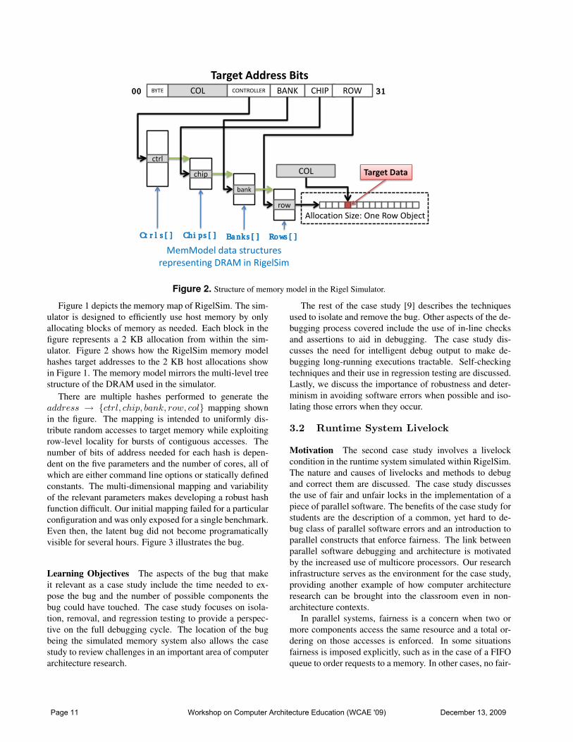
Figure 2. Structure of memory model in the Rigel Simulator.

Figure 1 depicts the memory map of RigelSim. The sim-ulator is designed to efficiently use host memory by onlyallocating blocks of memory as needed. Each block in thefigure represents a 2 KB allocation from within the sim-ulator. Figure 2 shows how the RigelSim memory modelhashes target addresses to the 2 KB host allocations showin Figure 1. The memory model mirrors the multi-level treestructure of the DRAM used in the simulator.

There are multiple hashes performed to generate theaddress → {ctrl, chip, bank, row, col} mapping shownin the figure. The mapping is intended to uniformly dis-tribute random accesses to target memory while exploitingrow-level locality for bursts of contiguous accesses. Thenumber of bits of address needed for each hash is depen-dent on the five parameters and the number of cores, all ofwhich are either command line options or statically definedconstants. The multi-dimensional mapping and variabilityof the relevant parameters makes developing a robust hashfunction difficult. Our initial mapping failed for a particularconfiguration and was only exposed for a single benchmark.Even then, the latent bug did not become programaticallyvisible for several hours. Figure 3 illustrates the bug.

Learning Objectives The aspects of the bug that makeit relevant as a case study include the time needed to ex-pose the bug and the number of possible components thebug could have touched. The case study focuses on isola-tion, removal, and regression testing to provide a perspec-tive on the full debugging cycle. The location of the bugbeing the simulated memory system also allows the casestudy to review challenges in an important area of computerarchitecture research.

The rest of the case study [9] describes the techniquesused to isolate and remove the bug. Other aspects of the de-bugging process covered include the use of in-line checksand assertions to aid in debugging. The case study dis-cusses the need for intelligent debug output to make de-bugging long-running executions tractable. Self-checkingtechniques and their use in regression testing are discussed.Lastly, we discuss the importance of robustness and deter-minism in avoiding software errors when possible and iso-lating those errors when they occur.

3.2 Runtime System Livelock

Motivation The second case study involves a livelockcondition in the runtime system simulated within RigelSim.The nature and causes of livelocks and methods to debugand correct them are discussed. The case study discussesthe use of fair and unfair locks in the implementation of apiece of parallel software. The benefits of the case study forstudents are the description of a common, yet hard to de-bug class of parallel software errors and an introduction toparallel constructs that enforce fairness. The link betweenparallel software debugging and architecture is motivatedby the increased use of multicore processors. Our researchinfrastructure serves as the environment for the case study,providing another example of how computer architectureresearch can be brought into the classroom even in non-architecture contexts.

In parallel systems, fairness is a concern when two ormore components access the same resource and a total or-dering on those accesses is enforced. In some situationsfairness is imposed explicitly, such as in the case of a FIFOqueue to order requests to a memory. In other cases, no fair-


Core A

Core B

Core C

spin_lock(LOCKlocal) Find Local Queue Empty spin_unlock(LOCKlocal)

spinning...spinning...

spinning... spinning...

HAS TASKS! Starving waiting for LOCKlocal

Figure 4. Timeline of cores participating in the livelock.Note that core A can never enqueue tasks because it is con-tinually starved for locklocal by B and C.

ness guarantees are given, such as the use of a simple spinlock for protecting a critical section in a parallel application.In the initial implementation of the runtime presented in thecase study, the lack of fairness led to two threads starvinga third, resulting in livelock. The case study examines howsuch a situation can occur and how to correct it by enforcingfairness explicitly.

Description and Debugging Process The runtime usedin the case study is a multi-level hierarchical work queuestructure. Tasks are inserted in the top level queue and areremoved from the low level queues. Here we will assumetwo levels of queue, a local and a global level. When alocal queue runs out of tasks, the core attempting to de-queue requests more tasks from the global queue. All queuemanagement is performed in software by the runtime us-ing atomic load-linked and store-conditional primitives pro-vided by the architecture.

Figure 4 shows the timeline of events that leads to live-lock when unfair locks are used. There are two locks in-volved. One lock must be held to access the local queue.The other lock must be held to access the global queue whenthe local queue runs out of work. To allow simultaneousenqueue and dequeue operations the local lock, locklocal, isdropped while attempting to access the global queue. Thelivelock occurs when two cores, B and C in the diagram,continually attempt to obtain tasks from an empty localqueue and thus starve A that is trying to obtain the locklocal

so that it can insert more tasks.

Learning Objectives The value of the case study for stu-dents is that they can see how a transient parallel softwareerror can be removed from a large system under simulation.The case study also discusses locking mechanisms and thetradeoffs inherent to fair versus unfair mechanisms. An-other valuable insight is that not all software errors resultin crashes or deadlocks that hang. Some software errors,such as livelocks, can reduce the system’s performance un-beknownst to the developer resulting in disappointing per-formance and misplaced optimization efforts.

4 Performance Analysis Case Study

In large-scale hardware and software systems correct-ness is often the primary concern for the developer. How-ever, for commercial applications and high-performancecomputing systems performance is a critical concern forcompetitive, economic, and tractability reasons. Introduc-tory programming and software engineering classes stresscorrectness while more advanced computer science coursesfocus on algorithmic complexity. However, optimizationis introduced to students late in their careers or not at all.Therefore, a disparity exists between the set of skills stu-dents have and the requirements of potential employers.

As multicore processors have become prevalent, parallelprogramming has been cited as a way to achieve higher per-formance for parallelizable applications [7]. While teachingparallel programming is one approach to training student todevelop faster code, there is still substantial performanceto be gained from sequential optimizations, which apply toboth sequential and parallel applications alike. As an ex-ample, one case study shows orders of magnitude speedupfor dense matrix multiply by applying algorithmic and se-quential optimizations [2]. Moreover, Moore’s Law aloneis unlikely to reduce single-threaded runtime, thus placingmore emphasis on sequential performance tuning [12] as ameans to increase performance for sequential applications.In light of this, we present experiences optimizing a largesequential application, a C++ based simulator we use in ourresearch, and discuss the use of these examples in under-graduate instruction.

4.1 Sample-based Profiling

A naıve approach to achieving higher performance isto develop many variants of an application and benchmarkeach to select the optimal design. Optimization by bench-marking alone is a time consuming process and achievessuboptimal results. Moreover, the N-version programmingapproach lacks directed feedback mechanisms to isolatewhere performance is being lost and masks performancedegradation located in code and libraries common acrossbenchmark versions.

A more methodical approach is to use sample-basedprofiling tools to target pathologies in large software sys-tems. Sample-based profiling allows the developer to iso-late performance problems and perform targeted optimiza-tions. This section describes how we used performance re-gressions from our architectural simulator. We use sample-based profiling to diagnose such regressions and to performtargeted optimizations.

Many profiling, instrumentation, and analysis tools arefreely available. Examples include the GNU profiler [8](gprof), Oprofile [1], and Intel’s PIN [13]. Each of these


tools was used at some point in the class; however this sec-tion focuses on our use of Oprofile. Oprofile is a suite oftools available on Linux systems that utilize the hardwareperformance counters on x86 hardware to perform low-overhead sample-based profiling.

4.2 Strength Reduction

Motivation Optimizing compilers have evolved to a pointwhere developers now rely almost exclusively on automa-tion to perform code generation. In most cases, hand-optimized assembly provides marginal performance gainsand large productivity and portability losses compared to astate-of-the-art compiler. Many computer science programsespouse this viewpoint and teach students high-level lan-guages. However, in doing so students may be unaware ofthe connection between statements in high-level languagesand the instructions that they generate and memory alloca-tion patterns [5, 6].

One approach to demonstrating the performance charac-teristics of high-level constructs in low-level or high-levellanguages is through performance analysis. As an exam-ple, a compiler for a high-level language, such as the GNUC++ compiler, can fail to optimize obvious cases. However,these cases may contribute little to overall runtime com-pared to caching effects and algorithm choices and thus notresult in observable performance degradation. However, ifsuch a case falls into a common code path, performance cansuffer greatly. The performance analysis applied to our sim-ulator provides a concrete illustration.

Description and Debugging Process Oprofile provides autility to annotate source code with relative frequency of ex-ecution for each line. While analyzing the annotated sourcefor RigelSim, we found that in many places 1-2% of runtimewas spent doing integer divides. The sum of these over-heads resulted in 5-8% slowdown across our benchmarks.Note that integer divide latencies on modern microproces-sors can be as as high as 79 cycles [3].

In RigelSim, many common operations such as addresshash functions involve integer multiplication, division, andmodulus operations with operands known at compile-timeto be powers of two. This enables a well-known opti-mization called strength reduction whereby expensive op-erations can be converted statically to logical shifts and bit-wise masks, thus saving dozens of cycles of latency. Thecompiler was not performing this optimization. However,we were able to remove most of the overhead by perform-ing the strength reduction at the C++ source level.

Learning Objectives The compiler example illustratesfour points that are valuable for students. The first is thatwhile compilers are quite good at generating high-quality

code, they are not infallible and choices at the source levelcan impact code generation in measurable ways. The sec-ond is that benchmarking alone cannot easily detect all per-formance pathologies. In this case we did not even realizethat there was a performance issue until we looked at theannotated source code. The example also illustrates thatmethodical approaches to performance debugging can leadthe developer, working at the source level, to the underly-ing cause of a performance pathology, which happen to beat the instruction level in this example. Lastly, a naıve ap-proach may have been to remove all modulus and divideoperations. Doing so would have reduced code readability,possibly introduced bugs, and would have been unnecessaryin almost all cases since most static divide instructions areexecuted few times dynamically in RigelSim.

4.3 Cache Blowout

Motivation The previous example used the number ofcommitted instructions and halted clock cycles to determinewhen to take samples. While this works well in most cases,some performance pathologies are not localized and are noteasily detected using instruction frequency-based sampling.One example from our simulator was the use of structureson the host side that track each miss status handling register(MSHR) used in the unified L2 cache inside the target.

Description and Debugging Process There are 128 tar-get L2 caches in a full RigelSim simulation and 8–32MSHRs associated with each L2. In the initial implemen-tation, in every target cycle, each MSHR had its valid bitchecked. The MSHRs are tracked as an array of objects ateach L2 and thus use an array-of-structures (AoS) data lay-out. While AoS achieves good locality when many fieldswithin a single record are accessed in succession, AoS pro-vides little locality across a single field in multiple records.In this example, the valid flag, represented as a single bitin memory, requires that a full 64-byte cache line be pulledinto the host data cache for each access. The other 511 bitsof the line are of no use if the MSHR is invalid, whichis the common case. So in each simulated target cycle128 × 32 × 64b = 256 KB of data are brought into thedata cache to find a ready MSHR, blowing out both the hostL1 and L2 data caches.

Sample-based profiling of host data cache missesshowed there to be an abundance of misses whenever validbits in MSHRs would be accessed. As a solution, we addedfacilities to track all valid bits for a cache in a single bit-vector structure. All of the valid bits could then be accessedwithout bringing large amounts of unnecessary data into thehost’s cache.


Learning Objectives This example illustrates that perfor-mance pathologies can be systemic and simple performancemodels, such as those based only on instruction count, failto capture the behavior of large systems with caches. Theexample also illustrates a use of sample-based profiling be-yond just committed instructions. A similar approach couldbe used for branch mispredictions and instruction cachemisses to better isolate performance issues across moduleboundaries. The example shows that caching effects are areal problem for large software systems, but that with properanalysis and simple code changes, such as the SoA/AoSconversion performed here, some pathological cache behav-ior can be avoided.

4.4 STL Pitfalls

Motivation Software systems developers face a tradeoffbetween performance and programmer productivity, codereadability, and maintainability. The C++ standard templatelibrary [16] can provide productivity gains by not forcingdevelopers to re-implement common data structures and al-gorithms repeatedly. However, naıve use of STL, and li-braries with opaque interfaces in general, can result in de-graded performance. In this section we show how a misuseof the STL map container in RigelSim led to a performancedegradation of over 60%. We then discuss how we wereable to use sample-based profiling to isolate and remove theperformance regression.

Description and Debugging Process During the devel-opment of RigelSim, the target statistics collection code forRigelSim was replaced. The old model relied upon a structof counters that were incremented directly, making it dif-ficult to easily print and gate statistics generation at run-time. The new model would use text-based strings to iden-tify counters by name and could be instantiated automati-cally in the simulator. The implementation relied upon anSTL map that used strings as keys and kept 64-bit integersas values. We found that not long after we added the newprofiling facilities, simulator runtime more than doubled.

STL is used extensively for some of the more complexanalysis we perform and had never been a performance con-cern. We analyzed the annotated output produced by Opro-file and found that the majority of execution time was at-tributable to internal methods of the STL map implemen-tation and string constructors. To achieve better resolu-tion, we used Oprofile to obtain a call graph of the exe-cution showing cumulative runtime at each method invoca-tion. Here it became clear that RigelSim was spending halfits execution doing string compares to traverse the red-blacktree data structure used by the STL map implementation.

Learning Objectives While STL can save programmersa good deal of effort, this example points out the importanceof understanding the overhead of using a library and, if it iscostly, how often it will be used. The solution in our caseinvolved using an array of structs with statically constantidentifiers, implemented using an enumerated type mappingcounter names to array indices. The new implementationavoided the need for text-based compares and thus removedthe overhead. The trade off was additional programmer ef-fort in developing the statistics collection system and addedtime to add new counters. However, the 2× slowdown ofthe initial implementation makes the slightly more inconve-nient mechanism a better trade off in RigelSim.

The lesson demonstrated here is that while libraries andcontainer classes such as STL can provide gain in produc-tivity and a reduction in bugs, their use does not come with-out cost. The proper use of performance analysis tools, suchas the performance counter annotated call graph and sourcecode tools provided by Oprofile, are invaluable in isolatingperformance regressions.

4.5 Summary

We have shown how sample-based profiling can be in-troduced to senior undergraduates. We use a case study ap-proach, relying upon examples from our own research andexperiences applying freely-available analysis tools to ourown simulator infrastructure. The examples can help stu-dents to better understand software performance, while alsobuilding a better understanding of the link between softwareperformance and the underlying architecture.

5 Discussion

In the paper we have shown how computer systems in-frastructure can be used in the classroom through examples.In this section we discuss the value of using case studies tobring computer systems research into an instructional set-ting. We also discuss two of the high-level points we illus-trate in the paper. One point is the tension between differentsolutions and the second is the proper use of abstraction. Weconclude by motivating the use of real world examples fromcomputer systems research to connect theoretical conceptswith practical systems.

Tools such as compilers, operating systems, and sim-ulators represent large scale applications that the instruc-tor, teaching assistants, and research assistants working re-search projects are intimately familiar with. However, whilea graduate student or professor focusing on computer archi-tecture may be familiar with a wide variety of large softwaresystems that have code freely available, such as operatingsystems and compilers, seldom do they spend as much time


developing code for those systems as they do for simulatorsand related tools.

Using a simulator as an example application increasesstudents’ exposure to computer architecture research top-ics and methodology. Increased exposure can motivate stu-dents to investigate advanced courses or careers in the areaof computer architecture. The students in the class wherethese case studies were used were undergraduates pursuingdegrees in computer engineering. A variety of areas of in-terest within computer engineering were represented. See-ing the tools computer architects use for their research andthe methods used to debug and optimize those tools mayentice students to consider computer architecture in theirchoice of graduate school and in their job search.

When bugs manifest themselves in a large system, thereare trade offs between reimplementation and quick fixes.The trade offs involve performance, programmer effort, andthe probability of inserting or exposing new bugs with a pro-posed solution. In our case studies we show that in somecases targeted fixes were the proper solution. Examples in-clude the strength reduction performance regression exam-ple and the memory aliasing bug. In other cases, we showedthat structural changes were necessary, such as in the live-lock example where we had to reimplement locking mech-anisms to ensure forward progress.

Another trade off is the frequency versus cost in verifica-tion and validation techniques. It is important to understandthe cost of verification and at what level to apply verifica-tion techniques to achieve high performance while havinghigh confidence in the results and minimal occurrence ofbugs. As an example, future memory aliasing bugs canbe regression tested with a simple checker, but the simplesolution also requires too much time to be run with everysimulation. Instead, longer tests such as these are run atpredefined intervals such as when code is committed to oursource repository or in nightly regression tests.

We demonstrate that while abstraction can provide tangi-ble benefits, it can also mask performance and correctnessproblems; One example being the use of STL for perfor-mance counters in RigelSim. While the abstraction pro-vided by the STL map led to an easy solution, it createda performance regression. The use of proper analysis tools,such as Oprofile, can greatly reduce the difficulty in diag-nosing such performance regressions. It also has the ped-agogical benefit of making otherwise opaque abstractionstransparent. Transparency during instruction increases thestudents’ understanding of the underlying implementationof an interface, such as the STL container classes used inthis example.

Lastly, we find the use of real world examples of perfor-mance and correctness issues valuable for students. Com-puter science courses often teach the theoretical underpin-nings of pathological conditions such as livelock. However,

it may be difficult for students to make the connection be-tween dining philosophers and threads of computation rac-ing for a lock, thus failing to make forward progress. Fur-thermore, a theoretical understanding of computer systems,such as the asymptotic complexity of our STL containerclasses, may not always be sufficient for understanding per-formance implications in real systems. Case studies havethe advantage of making fundamental issues in computerscience tangible for students thus strengthening the connec-tion between theory and practice.

6 ConclusionAlthough few courses in a typical curriculum focus on

computer architecture, the observations made while devel-oping large scale software and hardware systems while pur-suing research in computer architecture can still be adoptedfor a wide range of classes. We believe that computer archi-tecture research and the process it entails can provide usefuland relevant material for use in the classroom. As we show,one way architecture research can be brought into the class-room is by example using case studies.

This paper explores the use of case studies in debuggingand performance analysis. The examples in this work arederived from our experience developing, debugging, andtuning our research infrastructure. We find that having inti-mate knowledge of the system used in classroom discussioncan greatly aid in instruction. The use of computer systemsinfrastructure exposes students to a large software systemand illuminates problems that are unlikely to be found inclass projects due to constraints on time and scope.

The use of case studies can provide students with a portalinto the world of computer architecture research and large-scale computer system design in general. Using real worldexamples gives credibility to the presentation of the casestudies. Lastly, we find that the impact of computer archi-tecture on the classroom need not stop at designing micro-processors. Instead, we can use the process of computersystem design as a vehicle for educating a wider audienceof students.

Acknowledgment

The authors would like to thank Matt R. Johnson and theanonymous reviewers for their helpful comments.

References

[1] Oprofile. http://oprofile.sourceforge.net.[2] S. P. Amarasinghe. Performance engineering of software

systems, lecture 1, 2008. Available Online: http://stellar.mit.edu/S/course/6/fa08/6.197/.

[3] AMD Staff. Software optimization guide for AMD family10h processors, May 2009. Revision 3.11.


http://oprofile.sourceforge.net

http://stellar.mit.edu/S/course/6/fa08/6.197/

http://stellar.mit.edu/S/course/6/fa08/6.197/

[4] R. E. Bryant and D. R. O’Hallaron. Computer Systems: AProgrammer’s Perspective. Prentice Hall, 2003. Website:http://csapp.cs.cmu.edu/.

[5] R. Dewar and O. Astrachan. Point/counterpoint cs educationin the u.s.: heading in the wrong direction? Commun. ACM,52(7):41–45, 2009.

[6] R. B. K. Dewar and E. Schonberg. Computer science ed-ucation: Where are the software engineers of tomorrow?CrossTalk: Journal of Defense Software Engineering, Jan-uary 2009.

[7] A. Ghuloum. Viewpoint face the inevitable, embrace paral-lelism. Commun. ACM, 52(9):36–38, 2009.

[8] S. L. Graham, P. B. Kessler, and M. K. Mckusick. Gprof: Acall graph execution profiler. In SIGPLAN ’82: Proceedingsof the 1982 SIGPLAN symposium on Compiler construction,pages 120–126, New York, NY, USA, 1982. ACM.

[9] J. H. Kelm. Anatomy of a bug, May 2009.https://netfiles.uiuc.edu/jkelm2/www/kelm-rigelsim-bug.pdf.

[10] J. H. Kelm. Case study: Rigel task model livelock, May2009. Available at: https://netfiles.uiuc.edu/jkelm2/www/kelm-rtm-livelock.pdf.

[11] J. H. Kelm, D. R. Johnson, M. R. Johnson, N. C. Crago,W. Tuohy, A. Mahesri, S. S. Lumetta, M. I. Frank, and S. J.Patel. Rigel: An architecture and scalable programming in-terface for a 1000-core accelerator. In Proceedings of the

International Symposium on Computer Architecture, June2009.

[12] J. Larus. Spending Moore’s dividend. Commun. ACM,52(5):62–69, 2009.

[13] C.-K. Luk, R. Cohn, R. Muth, H. Patil, A. Klauser,G. Lowney, S. Wallace, V. J. Reddi, and K. Hazelwood. Pin:building customized program analysis tools with dynamicinstrumentation. In PLDI ’05: Proceedings of the 2005ACM SIGPLAN conference on Programming language de-sign and implementation, pages 190–200, New York, NY,USA, 2005. ACM.

[14] S. S. Lumetta. ECE498SL Spring 2009 homepage,May 2009. http://courses.ece.illinois.edu/ECE498/SL/.

[15] Y. N. Patt and S. J. Patel. Introduction to Computing Sys-tems: From Bits and Gates to C and Beyond. McGraw-Hill, 2003. Class Website at the University of Illinois:http://courses.ece.illinois.edu/ECE190/.

[16] A. Stepanov and M. Lee. The standard template library.Technical Report X3J16/94-0095, HP Laboratories, Novem-ber 1995.

[17] B. Stroustrup. The design and evolution of C++. ACMPress/Addison-Wesley Publishing Co., New York, NY,USA, 1994.


http://csapp.cs.cmu.edu/

https://netfiles.uiuc.edu/ jkelm2/www/kelm-rigelsim-bug.pdf

https://netfiles.uiuc.edu/ jkelm2/www/kelm-rigelsim-bug.pdf

https://netfiles.uiuc.edu/ jkelm2/www/kelm-rtm-livelock.pdf

https://netfiles.uiuc.edu/ jkelm2/www/kelm-rtm-livelock.pdf

http://courses.ece.illinois.edu/ECE498/SL/

http://courses.ece.illinois.edu/ECE498/SL/

http://courses.ece.illinois.edu/ECE190/

Circuit Modeling in DLSim 3

Richard M. Salter, John L. Donaldson, Serguei Egorov, Kiron Roy

Computer Science DepartmentOberlin College

Oberlin, OH 44074

[email protected], [email protected], [email protected], [email protected]

Abstract

DLSim 3, is a GUI-based digital logic simulation pro-gram developed by Richard Salter at Oberlin College, ex-tends the capabilities of such programs through the use ofJava plug-ins. DLSim 3 makes it it possible to use the soft-ware for digital design at higher levels of abstraction. WithDLSim 3, we are able to present the many levels of circuitdesign in a single environment, from low level combina-tional and sequential circuits through models of completeCPUs. This paper shows how DLSim 3 has been used inthe classroom to model several CPUs well known to educa-tors, and to support creative efforts on the part of studentsof Computer Organization.

1 INTRODUCTION

Many excellent GUI-based logic simulation systemshave been developed and are available for download [1, 2, 3,5, 8]. These systems are very useful for studying basic com-binatorial and sequential circuits. While they generally allprovide some abstraction mechanism (“black boxes”) thatpermits circuit reuse, they are limited by their GUI basedenvironments to relatively small models.

DLSim 3 [9, 10, 4] joins this group but goes beyond theseefforts through its innovative use of Java plug-ins. A plug-in is a software module, written in Java, which is addedto DLSim’s design platform and can be used as a compo-nent in more complex circuit designs. The user can writeJava modules that simulate higher-level logic components(i.e., memories, registers, ALUs) which supplement DL-Sim’s collection of built-in components. The plug-in facil-ity is built around an interface that describes what functionsa plug-in must perform in order to be installed in the sys-tem, and an API of functions which support the writing ofplug-ins.

Plug-ins allow the simulator to scale up to whatever level

of abstraction is appropriate in a course. For example, at onestage in a course, students might be asked to design an ALUusing only logic gates. Later, when studying CPU design,the instructor might provide an ALU plug-in to be used as acomponent.

In addition, plug-ins can perform I/O, either GUI-oriented user interaction or file operations. For example, wehave written plug-ins which can load a microprogram froma file, store results of a simulation to a file, and provide aninteractive keypad for a simulated calculator.

The design philosophy behind DLSim was described bySalter and Donaldson in [10]. In this paper we describehow we have used DLSim to visually simulate the CPU de-signs of Patt and Patel [6] and Warford [12]. With thesedesigns, we have been able to illustrate important CPU de-sign concepts such as datapath construction and and controlunit design. In addition, we describe how we have used DL-Sim in the classroom in the Computer Organization courseat Oberlin.

2 Plug-ins

The power of DLSim 3 to model large-scale circuit com-ponents, such as RAM chips and CPUs, is achieved throughplug-ins. Plug-ins are described in detail in [10]. Here wegive a brief summary.

A plug-in is a Java class which represents a circuit com-ponent. Every plug-in is a subclass of DLPlugIn, whichgives it the basic structure it needs to fit into the DLSim 3simulation engine.

By default, DLSim 3 displays a plug-in as a rectanglewith inputs on the left and outputs on the right. The pro-grammer may, however, provide a customized view for theplug-in by writing a separate view class.

1


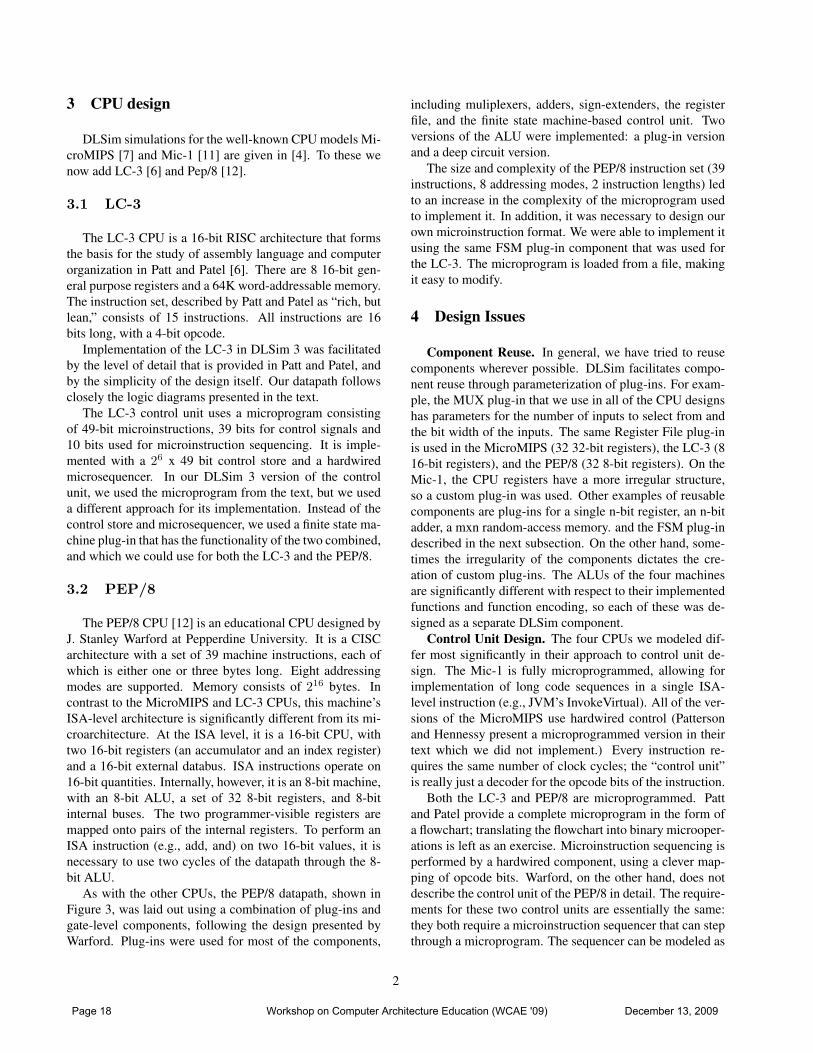
3 CPU design

DLSim simulations for the well-known CPU models Mi-croMIPS [7] and Mic-1 [11] are given in [4]. To these wenow add LC-3 [6] and Pep/8 [12].

3.1 LC-3

The LC-3 CPU is a 16-bit RISC architecture that formsthe basis for the study of assembly language and computerorganization in Patt and Patel [6]. There are 8 16-bit gen-eral purpose registers and a 64K word-addressable memory.The instruction set, described by Patt and Patel as “rich, butlean,” consists of 15 instructions. All instructions are 16bits long, with a 4-bit opcode.

Implementation of the LC-3 in DLSim 3 was facilitatedby the level of detail that is provided in Patt and Patel, andby the simplicity of the design itself. Our datapath followsclosely the logic diagrams presented in the text.

The LC-3 control unit uses a microprogram consistingof 49-bit microinstructions, 39 bits for control signals and10 bits used for microinstruction sequencing. It is imple-mented with a 26 x 49 bit control store and a hardwiredmicrosequencer. In our DLSim 3 version of the controlunit, we used the microprogram from the text, but we useda different approach for its implementation. Instead of thecontrol store and microsequencer, we used a finite state ma-chine plug-in that has the functionality of the two combined,and which we could use for both the LC-3 and the PEP/8.

3.2 PEP/8

The PEP/8 CPU [12] is an educational CPU designed byJ. Stanley Warford at Pepperdine University. It is a CISCarchitecture with a set of 39 machine instructions, each ofwhich is either one or three bytes long. Eight addressingmodes are supported. Memory consists of 216 bytes. Incontrast to the MicroMIPS and LC-3 CPUs, this machine’sISA-level architecture is significantly different from its mi-croarchitecture. At the ISA level, it is a 16-bit CPU, withtwo 16-bit registers (an accumulator and an index register)and a 16-bit external databus. ISA instructions operate on16-bit quantities. Internally, however, it is an 8-bit machine,with an 8-bit ALU, a set of 32 8-bit registers, and 8-bitinternal buses. The two programmer-visible registers aremapped onto pairs of the internal registers. To perform anISA instruction (e.g., add, and) on two 16-bit values, it isnecessary to use two cycles of the datapath through the 8-bit ALU.

As with the other CPUs, the PEP/8 datapath, shown inFigure 3, was laid out using a combination of plug-ins andgate-level components, following the design presented byWarford. Plug-ins were used for most of the components,

including muliplexers, adders, sign-extenders, the registerfile, and the finite state machine-based control unit. Twoversions of the ALU were implemented: a plug-in versionand a deep circuit version.

The size and complexity of the PEP/8 instruction set (39instructions, 8 addressing modes, 2 instruction lengths) ledto an increase in the complexity of the microprogram usedto implement it. In addition, it was necessary to design ourown microinstruction format. We were able to implement itusing the same FSM plug-in component that was used forthe LC-3. The microprogram is loaded from a file, makingit easy to modify.

4 Design Issues

Component Reuse. In general, we have tried to reusecomponents wherever possible. DLSim facilitates compo-nent reuse through parameterization of plug-ins. For exam-ple, the MUX plug-in that we use in all of the CPU designshas parameters for the number of inputs to select from andthe bit width of the inputs. The same Register File plug-inis used in the MicroMIPS (32 32-bit registers), the LC-3 (816-bit registers), and the PEP/8 (32 8-bit registers). On theMic-1, the CPU registers have a more irregular structure,so a custom plug-in was used. Other examples of reusablecomponents are plug-ins for a single n-bit register, an n-bitadder, a mxn random-access memory. and the FSM plug-indescribed in the next subsection. On the other hand, some-times the irregularity of the components dictates the cre-ation of custom plug-ins. The ALUs of the four machinesare significantly different with respect to their implementedfunctions and function encoding, so each of these was de-signed as a separate DLSim component.

Control Unit Design. The four CPUs we modeled dif-fer most significantly in their approach to control unit de-sign. The Mic-1 is fully microprogrammed, allowing forimplementation of long code sequences in a single ISA-level instruction (e.g., JVM’s InvokeVirtual). All of the ver-sions of the MicroMIPS use hardwired control (Pattersonand Hennessy present a microprogrammed version in theirtext which we did not implement.) Every instruction re-quires the same number of clock cycles; the “control unit”is really just a decoder for the opcode bits of the instruction.

Both the LC-3 and PEP/8 are microprogrammed. Pattand Patel provide a complete microprogram in the form ofa flowchart; translating the flowchart into binary microoper-ations is left as an exercise. Microinstruction sequencing isperformed by a hardwired component, using a clever map-ping of opcode bits. Warford, on the other hand, does notdescribe the control unit of the PEP/8 in detail. The require-ments for these two control units are essentially the same:they both require a microinstruction sequencer that can stepthrough a microprogram. The sequencer can be modeled as

2


Figure 1. LC-3 Data-path (subsection)

Figure 2. Pep/8 ALU

3


Figure 3. Pep/8 Data-path (subsection)

a finite state machine (FSM), which we implemented as aplug-in which is used for the control units of both the LC-3and the PEP/8. The inputs of the FSM are the clock andseveral feedback lines; its outputs are the control signals.Internally, it keeps a state register (actually just a Java vari-able) to maintain the current state of the FSM, a transitiontable for the FSM, and an output table. The microprogramis loaded into the tables from a file prior to starting the ma-chine simulation.

Plug-ins vs. Deep Circuits. DLSim 3 provides twoways to scale a design up to large-scale circuits. In additionto the plug-in facility, it is possible to build larger circuitsusing only basic gates by building several layers of progres-sively more complex components, using the card and chipabstractions described in [10]. We call this the deep circuitapproach. A good example of this is found in the designof an ALU. It is complex enough to warrant a layered ap-proach, but not so large that it would overwhelm the simu-lator if implemented at the gate level.

The ALUs of both the Mic-1 and the PEP/8 have beenimplemented both as plug-ins and as deep circuits. Figure 2illustrates the deep circuit version of the PEP/8 ALU. Eachbox in the figure is a functional component performing adifferent operation: And, Or, Add/Subtract, etc. Clickingon any of these components will show a deeper circuit dia-gram, illustrating how it is designed using lower-level com-ponents, and so on, until all of the components are com-

prised only of gates.Both approaches have pedagogical value. With a deep

circuit, the hierarchical view of digital design is made clear.With a plug-in, the focus can be placed on the functionalityof a component as a black box, while hiding the details ofits implementation.

5 DLSim in the Classroom

At Oberlin College, the computer organization courseis offered once per year and covers binary and hexadeci-mal arithmetic, digital logic, assembly language program-ming, and microarchitecture/microprogramming. The dig-ital logic unit lasts about 3 weeks, with one homework as-signment using DLSim to construct a circuit. Because ofDLSim 3’s capacity to model a complete CPU, it is alsobeing used in the microarchitecture unit of the course todemonstrate the Mic-1.

5.1 Computer Organization Assignment

DLSim 3’s plug-in feature has allowed for a more cre-ative approach to the circuit design assignment. Studentswere provided with plug-ins used to model visual displayelements and drivers, such as color tiles and LED displays.They were required to implement a periodic display con-

4


Figure 4. Traveling Sign (with marquee)

Figure 5. Dice

5


a) b)

Figure 6. Fireworks Generator: a) top level; b) main circuit

sisting of either a moving or flashing sign or a color dis-play. The display could include randomness, but could notbe simply random; i.e. it had to have some periodic repeti-tion that required the implementation of a counter.

The students received a plug-in archive containing thefollowing display elements:

• LEDDriver: a component that forms letter and nu-meral patterns on a 7-segment LED;1

• Pixel and SuperPixel: a tile that displays, respec-tively, 8 and 224 different colors;2

• PRNG: a pseudo-random number generator;

• FSM: a finite-state-machine-based control unit.

As an example of the moving sign, the students weregiven the circuit shown in Figure 4. The 16 LEDDriverscan be seen in the upper left part of the figure. The spin-ners in the LEDDrivers allow the user to program the sign’smessage. In addition to the sign itself, which uses DLSim7-segment display components, colored tiles (SuperPixels)appear above the message. Each tile’s color is determinedby the bits used to configure the letter appearing in the cor-responding LED. The colors move with the letters, fromright to left, producing a “marquee” effect. Note that thecontrol logic for this circuit is contained in the travsign and

1The 7-segment LED is a standard component in DLSim.2Initially only the Pixel was distributed; the SuperPixel was added by

popular demand.

ctr4 chips; consequently this circuit could be distributed tostudents as a live example without also providing a solutionto the assignment.

A second example is shown in Figure 5. The display is asquare of 9 Pixel plug-ins that rotate through a “dice”-likepresentation of the numbers 1 - 6. Each number is displayedusing a different color from the 3 primary (red, green, blue)and 3 secondary (cyan, yellow, magenta) colors displayableby a Pixel plug-in. Once again, the dicedemo chip allowsthis circuit to be safely distributed.

5.2 Results

The resulting student projects were ambitious andshowed great design ingenuity. (Running version can beviewed as applets at http://www.dlsim.com/demos.html .)They include a sign that flashes in a periodic pattern and acolor “snake” that travels through a square display. Here isthe description of a DLSim Fireworks Generator shown inFigure 6.

This circuit simulates exploding fireworks. Itconsists of a counter which turns on a singlebit from the LSB to the MSB of 8 bits in se-quence. The counter is modified so that the finalJK flip flop does not feed back to the first. Thiscauses the circuit to switch between 01010101and 10101010 when the first flip flop’s input is0. The circuit implements a control which allows

6


the user to ”shoot” a firework. This causes thefirst flip flop to output a 1, then a 0, then a 1, andso on until the shoot button is turned off. The al-ternating 1’s and 0’s ripple through the rest of theflip flop outputs. The flip flop outputs are sentto circuits which trigger random number gener-ators, then filter out 0s, then gate the output sothat 0 is output unless the specific flip flop is out-putting 1. This number is then sent to a pixel.Each pixel represents a ring of the firework, withthe top pixel representing the center ring.

Motivated by the high impact of the display elements, stu-dents lent their creative energies to designing unusually so-phisticated circuits. They organized their designs in a hi-erarchical fashion, and showed uncharacteristic patience infashioning their designs into running models.

5.3 Advanced Course

Beyond the Computer Organization course, DLSim 3 isappropriate for use in independent student design projectsand more advanced courses. We have supervised severalstudents in a variety of projects which were described indetail in [4]:

• writing a cache memory plug-in and interfacing it tothe MicroMIPS processor model;

• designing a hand calculator which used the Mi-croMIPS for its computations. This project involvedwriting a plug-in to represent the calculator keypad anddisplay, and interfacing it to the processor;

• writing a plug-in to represent a PLA;

Oberlin also offers an upper-division elective in ComputerArchitecture which covers topics such as pipelining, cachememory, and multiprocessor design. Because the course isnot offered on a regular basis, we have not yet had the op-portunity to use the new features of DLSim 3 in the course.We do anticipate, however, that DLSim 3 will prove to beuseful in teaching the course in the future. In particular,our model of a pipelined version of the MIPS processor,described in [4], will be especially valuable in illustratingconcepts such as data and control hazards, stall cycles, andforwarding.

6 Conclusion

DLSim 3 is a highly versatile software tool designed forthe design and simulation of digital logic circuits. Throughits use of software plug-ins, it is capable of simulating dig-ital circuits of varying levels of complexity. The exam-ples presented in this paper demonstrate some of the ways

that DLSim 3 can be used as a pedagogical aid in Com-puter Organization courses. We have been successful in us-ing it to simulate the CPU designs presented in the popu-lar textbooks of Tanenbaum, Patterson and Hennessy, Pattand Patel, and Warford, in order to demonstrate a variety ofimplementation techniques; for example, hard-wired con-trol, microprogramming, and pipelining. DLSim 3 has alsostrongly motivated students to produce their own creativecircuit designs. We intend to continue to expand our libraryof plug-ins and circuits, which are available, along with theDLSim 3 software, at our website, www.dlsim.com.

References

[1] D. L. Barker. Digital works 3.0. http://matrixmultimedia.com/datasheets/eldwk.pdf, 2006.

[2] C. Burch. Logisim: A graphical system for logic circuitdesign and simulation. J. Educ. Resour. Comput., 2(1):5–16, 2002.

[3] C. Burch. Logisim 2.1.6. http://ozark.hendrix.edu/ burch/logisim,2007.

[4] J. L. Donaldson, R. M. Salter, A. Singhal, J. Kramer-Miller,and S. Egorov. Illustrating CPU design concepts using DL-Sim 3. In FIE’09: Proceedings of the 39th ASEE/IEEEFrontiers in Eduction Conference, pages T4G–1 – T4G–6.ASEE/IEEE, October 2009.

[5] A. Masson. Logicsim. http://wuarchive.wustl.edu/edu/math/software/mac/LogicSim/, 1996.

[6] Y. N. Patt and J. J. Patel. Introduction to Computing Sys-tems: From Bits and Gates to C and Beyond, 2nd Edition.McGraw-Hill, New York, 2004.

[7] D. A. Patterson and J. Hennessy. Computer Organizationand Design, 3rd Edition. Morgan Kaufmann, Palo Alto, CA,2004.

[8] D. A. Poplawski. A pedagogically targeted logic designand simulation tool. In WCAE’07, Proceedings of the 2007workshop on Computer architecture education, pages 1–7,June 2007.

[9] R. M. Salter and J. L. Donaldson. Using DLSim 3: a scal-able, extensible, multi-level logic simulator. In ITiCSE’08:Proceedings of 13th Annual Conference on Innovation andTechnology in Computer Science Education, page 315.ACM Special Interest Group on Computer Science Educa-tion, June – July 2008.

[10] R. M. Salter and J. L. Donaldson. Abstraction and extensi-bility in digital logic simulation software. In SIGCSE ’09:Proceedings of the 40th ACM technical symposium on Com-puter science education, pages 418–422, New York, NY,USA, 2009. ACM.

[11] A. S. Tanenbaum. Structured Computer Organization, 5th

Edition. Prentice-Hall, Upper Saddle River, NJ, 2006.[12] J. S. Warford. Computer Systems, 4th Edition. Jones and

Bartlett, Boston, 2010.

7


A Two-tiered Modelling Framework for Undergraduate Computer ArchitectureCourses

Jason LoewDepartment of Computer Science

State University of New York at Binghamton

Dmitry PonomarevDepartment of Computer Science

State University of New York at Binghamton

Abstract

We describe a new methodology for modelling key mi-croarchitectural features in an advanced undergraduatecomputer architecture course and demonstrate the specificapplication of this methodology to branch predictors. Theproposed approach consists of two separate, but synergis-tic programming assignments. In the first part, studentsimplement the branch prediction logic as an independentsoftware module, but the interfaces are defined in such away that the developed code can be easily integrated into acycle-accurate simulator. In the second part, such integra-tion into the M-Sim simulator takes place. Such decouplingallows the students to focus on the features of the branchpredictor in isolation from rather complex simulator code.In addition, the two-stage process also better aligns itselfwith the class schedule, because the students are only ex-posed to the simulator code at the end of the semester, afterthey learned most of the key design concepts that are sup-ported in the simulator.

In this paper, we present the details of both assignmentsand also describe the modifications introduced to the M-Simsimulator to support such modelling capabilities. All as-signments and the modified simulator are available onlineand the framework has already been used in the undergrad-uate computer architecture course at SUNY Binghamton.Finally, the proposed framework can be easily extended formodelling other key architectural paradigms, such as regis-ter renaming and caches.

1 Introduction and Motivation

Several key microarchitectural concepts used in mod-ern processor design (branch prediction, register renaming,cache memories) are fairly easy to understand conceptually,but the real appreciation of the internal operations of thesemechanisms can only be achieved if one tries to model andimplement these subsystems using various simulation and

design automation tools. This is why it is extremely impor-tant to augment the theoretical underpinnings with a solidexperimentation methodology to provide students with suf-ficient hands-on experience. The key challenge for usingsuch modelling in the undergraduate courses is that the stu-dents often do not have sufficient expertise and time to usethe tools typically designed for research. In this paper, weintroduce a novel way to approach this problem and we il-lustrate our approach using dynamic branch prediction logicas an example of a subsystem to be modelled.

Dynamic branch prediction is among the most funda-mental concepts in modern processor design. It is also an in-tegral part of any advanced undergraduate computer archi-tecture course. While the fundamental concepts and ideasof basic dynamic branch prediction logic are straightfor-ward and can be fairly easily explained to an undergradu-ate class using a few powerpoint slides, the main challengeslie in supporting these basic concepts with adequate hands-on exercises that would allow the students to reinforce thetheoretical fundamentals. This reinforcement is especiallyimportant in the field of computer architecture, because thereal performance impact of any design can only be gaugedby observing the processor’s behavior (with the hardwareadditions being evaluated) on a set of standard benchmark-ing programs. The easiest way to accomplish this is by us-ing cycle-accurate simulators.

Cycle-accurate simulations represent the primary vehicleof early-stage evaluations of key architectural ideas, bothin academia and in the industry. A large number of open-source simulators, some of them specifically designed forthe use in academia, are widely available [1, 3, 6, 8, 7].Unfortunately, most of these simulators are designed for re-search activities and are of limited use in education, espe-cially at the undergraduate level. The main reason is thatit takes a significant amount of time and familiarity withthe discipline to understand how these simulators work, andin some cases even simply to be able to run them. Forexample, the simulators almost never employ ”execute-at-execute” model, where instructions would actually be exe-cuted out-of-order, as they would on a real hardware. In-


stead, ”execute-at-decode” model is used, where the in-structionsare actually executed at the same time they aredecoded (in-order), and the out-of-order effects are mod-elled through rather complex manipulations with auxiliarystructures, such as the Register Update Unit (RUU) usedin Simplescalar simulator [1]. While such tools are cer-tainly suitable for advanced PhD students involved in re-search projects (who can afford the learning curve involvedin using the simulators), and even for some simple projectsin graduate architecture courses, they are too complex foran average undergraduate student. Indeed, it is unreason-able to spend a significant amount of time learning aboutthe simulator’s intricacies just to carry out one or two as-signments. Even though the branch prediction code is usu-ally somewhat isolated from the rest of the simulator code,the interface is still rather non-trivial for the undergradu-ate students and the students still need to understand largechunks of highly-optimized C code to complete even thesimplest assignments. In summary, the main problem stemsfrom the absence of an intermediate step, where the studentscould easily understand the branch predictor interface andinternal organization and functionality, and then seamlesslyincorporate it into the full-fledged simulator. In this paper,we describe such a two-tiered framework, which we suc-cessfully integrated into the CS325 (Advanced ComputerArchitecture) course at SUNY Binghamton.

Our proposed framework for supporting experimentswith dynamic branch predictors in undergraduate computerarchitecture course consists of two assignments (both ofwhich are presented in detail in the subsequent sections).The first part is a simple programming assignment that pro-vides the students with all the interfaces to the dynamicbranch predictor, including the input trace of branch in-struction outcomes to be fed into the predictor. Students areasked to fill in the body of the functions (bpredupdate andbpredlookup) to implement a particular prediction mech-anism(such as gshare [4]). Evaluation is performed us-ing a trace of supplied branch instruction PC addresses andcorresponding branch outcomes. This is implemented as astandalone piece. The second part of our framework is theintegration of this code into a modified M-Sim simulator[3]. M-Sim is a redesigned version of Simplescalar sim-ulator, that supports simulation of multithreaded and mul-ticore architectures, and also explicitly models register re-naming, load-hit speculation, replays and a variety of otherfeatures. For this assignment, the branch prediction im-plementation of M-Sim has been completely rewritten toseamlessly support the interface provided to the studentsin the first assignment. In essence, the students can sim-ply ”drop” the code that they developed during the first as-signment into the modified M-Sim, and end up with thebranch predictor implementation that can be driven by theactual outcomes of the branches executed within SPEC pro-

grams. The main benefit of the proposed approach is that itallows the students to abstract the details of the simulatorand focus instead on the logic pertaining to the operationof the branch predictor. The modified M-Sim code sup-porting this framework is available at the following URL:http://www.cs.binghamton.edu/∼msim/branch

Another advantage of using such a multi-step approachis that it aligns more naturally with the course schedule interms of giving the simulator code to the students only atthe time when most of the advanced concepts implementedin the simulator are already covered during the lectures. Forexample, consider a typical Fall semester schedule for anundergraduate architecture course taught based on Pattersonand Hennessy’s book [5]. Typically, the first several weeksof the course are spent on the topics such as performancemetrics, ISA design, advanced arithmetic and non-pipelineddatapath and control logic design. Pipelined execution, for-warding and branch prediction are the first advanced topicscovered, and this usually happens sometime around mid-way point of the semester (mid-October). At this time, itis too early to introduce the students to the simulator, be-cause most of the advanced concepts implemented in thesimulator (register renaming, out-of-order execution, cachehierarchies) are not yet explained during the lectures. Inthis case, the students would have a double burden of tryingto implement a new branch prediction design in a simulatorthat supports extensive functionality, much of it they do notyet understand. In contrast, if a simple self-contained pro-gramming assignment (as detailed in Section 2) is given atthis point, the students would already know enough infor-mation to implement the prediction and update logic with-out having to get concerned with the details of the rest of thepipeline stages. If this assignment takes 2-3 weeks to com-plete, then sometime around the middle of November, thestudents can be introduced to the simulator to complete thesecond part of the branch prediction modelling assignment.By that time, all the key concepts implemented within thesimulator would already be covered and it would be mucheasier for students to work with the simulator.

The rest of the paper is organized as follows. Section 2describes the first programming assignment for modellingbranch prediction logic without the use of full-fledged sim-ulators. Section 3 provides a short overview of the M-Sim-3.0 simulator. Section 4 describes the second assignment,where the code designed in the first assignment is seam-lessly integrated into M-Sim simulator. Finally, we con-clude in Section 5.

2 First Programming Assignment

The first portion of the modelling framework, describedin this section, encompasses all of the programming work,but allows the branch predictor code to be implemented out-


side of the simulator and in the form of a standalone pro-grammingassignment. In this assignment, which can begiven out right after the branch prediction fundamentals arecovered in class, the students are given the base class branchpredictor code and a set of other files that are required forimplementation and testing. The students are also providedwith examples in the form of the two stateless predictors- ”always taken” and ”always not taken”. A driver (im-plemented through main.c file) feeds the trace file to thepredictors and collects the prediction results. In the follow-ing subsections, we describe the details of the trace file andthe interfaces that the students are asked to work with. Thegoal of this assignment is to implement a specific predictionlogic in the framework of the defined interfaces.

2.1 A Generic Branch Predictor Model

A generic dynamic branch predictor model would havethe following components:

• Counters: Various counters keep track of the statisticsof the predictor. Students will generally need to keeptrack of the number of lookups and hits/misses.

• reset(): Resets the counters after fast-forwarding. Stu-dents do not need to implement this unless they addtheir own counters.

• retstack: The return address stack. If left unimple-mented, it does nothing.

• Constructors: These create the branch predictor. Stu-dents should generally see an example of how thesework.

• bpredlookup: The lookup abstraction that students aretaught.

• bpredupdate: The update abstraction that students aretaught.

• bpredreg stats: Adds the counters to the simulator’sstatisticsdatabase. Can be ignored unless the studentsneed to track their own counters.

2.2 Trace File Format

The trace file contains the set of branch predictor lookuprequests and the set of branch predictor update requests(generated based on the actual branch outcomes during pro-gram execution) that are generated by a hypothetical pro-gram. The format of each of these requests is shown in thetable below. For this assignment, we ignore the issues asso-ciated with managing return address stack.

• Lookup: lookup <branchPC> <branchtarget ifknown> <opcode> <iscall> <is return>

• Update: update <branchPC> <branchtarget><opcode>

The contents of this trace file are used as an input to thepredictor that the students are asked to design.

The easiest way to generate realistic trace files is toproduce them from M-Sim directly (although, it is alsopossible to create them in some other manner). This canbe accomplished by adding code before bpredlookup andbpredupdate are called. For bpredlookup, we output”lookup” followed by thebranch addressandbranch tar-get address(both in hex, prefixed with 0x) then we outputtheopcodeand the flagsis call andis return. These can becopiedstraight out of the call to bpredlookup (or done oncein bpredlookup). For bpredupdate, we output ”update”followed by thebranch addressandbranch target address(both in hex, prefixed with 0x) then we output theopcode.The driver provided in main.c file determines the values oftaken,pred takenandcorrectand supplies those to the pre-dictors.

Students generally find it difficult to craft the code to testtheir implementations. When using trace files, a ”boiler-plate” is provided that includes:

• A makefile that compiles all of the required files.

• A driver (such as main.cpp) that runs their code.

2.3 Data Structures and Predictor Inter-faces

2.3.1 Data Structures

Appropriate data structures need to be designed to representthe predictor state. This can be managed in any reasonableway within the constructs of the class. Data structures canbe created within the class constructor which must call thebase constructor with the predictor’s name. This is shown atthe top of Figure 1 using a standard initializer list approach.Any size requirements (such as power of 2) should be en-forced here. Initialization of the predictor with some start-ing values is also done here. A destructor is only needed ifthe students use their own memory management. It is suit-able to allow them the use of existing STL structures suchas vector.

2.3.2 The Lookup Interface

Branch predictor lookup procedure takes the address of thebranch instruction (mdaddr t baddr) and the target address(md addr t btarget) in order to make a prediction. Studentsmust additionally handledir updateptr which is cleared


during lookup and has a pointer (pdir1) that points to theentry used by the branch predictor. The other arguments(op, is call, is return, stackrecoveridx) can be ignored bystudentsat the discretion of the instructor. The number oflookups is maintained here.

2.3.3 The Update Interface

Branch predictor update procedure takes the address of thebranch instruction (mdaddr t baddr), the target address(md addr t btarget) and dirupdateptr (dir updateptr->pdir1) to update the branch predictor state. The result ofthe branch comes from the remaining parameters (opcan beignored).takenis a boolean that tells us what the branch ac-tually did. pred takentells us the prediction that was made.correct indicates if address prediction was correct (this isoptional for students). Misses/hits and most other perfor-mance statistics are maintained here.

2.4 Statistics

Each branch predictor maintains statistics related to itsown performance and these stats are printed to the screen atthe end of simulation. The relevant statistical counters arecontained in the parent branch predictor class, which reg-isters the statistics with the database, identical to the onemaintained in the M-Sim simulator. The database was in-cluded explicitly as part of this assignment in order to makefuture transition to M-Sim (as described in Section 4) easier.The statistics handling is already built in and students cansimply increment/adjust the counters that are provided bythe parent class. Students can add their own statistics, butthis is neither required, nor necessary for this assignment.

2.5 Examples for Students

Students will often find it helpful to have an exampleto start with. The stateless predictors (always taken, nevertaken) can be provided to students for this purpose. Thestateless predictors show how minimal the interface can beand provide an example of how to use the existing compo-nents that are inherited from the base branch predictor class.See Figure 1.

2.6 The Assignment

The complete assignment package, includingtrace files, is available at the following URL:http://www.cs.binghamton.edu/∼msim/branch

Students need to download the code package providedby the instructor, unpack the code and execute the ”make”command. The code is executed as follows: ”./main.exegcc.trace” where gcc.trace can be replaced with any other

#include”bpredtaken.h”#include<cassert>

bpredbpredtaken::bpredbpredtaken():bpred t(”taken”){}

md addr tbpred bpredtaken::bpredlookup(

md addr t,md addr t btarget, //branch target, if takenmd opcode op, //opcode of instructionbool, bool,bpredupdatet *dir updateptr, //pred state pointerint*)

{assert(dirupdateptr);

if(!(MD OP FLAGS(op) & F CTRL)){

return 0; //If not a control inst}lookups++;dir updateptr->dir.ras = false; //Clear dir updateptrdir updateptr->pdir1 = NULL;dir updateptr->pdir2 = NULL;dir updateptr->pmeta = NULL;

return btarget;}

voidbpredbpredtaken::bpredupdate(

md addr t,md addr t,bool taken, //non-zero if branch was takenbool predtaken, //non-zero if branch was pred takenbool correct, //was earlier prediction correct?md opcode op, //opcode of instructionbpred updatet *dir updateptr) //pred state pointer

{if(!(MD OP FLAGS(op) & F CTRL)){

return; //If not a control inst}

addrhits += correct; //Update statsdir hits += (predtaken == taken);misses += (predtaken != taken);

if(dir updateptr->dir.ras) //If return address stack used{

usedras++;rashits += correct;

}

if(MD IS INDIR(op)) //If indirect jump{

jr seen++;jr hits += correct;

if(!d ir updateptr->dir.ras){

jr non rasseen++;jr non rashits += correct;

}else{

//used return address stack, donereturn;

}}

}

Figure 1. Always Taken Predictor


.tracefile. The first time this is executed, the program willrun and provide results for the ”always taken” branch pre-dictor. The students need to provide their own<GIVENTYPE>predictor in the form of the filesstudent.candstu-dent.h. These should be modelled after the predictors pro-vided (the skeleton provided in the package can be givento students). No other files need to be modified. Figure 2shows the complete formulation of the assignment, as usedin CS325 at SUNY Binghamton in the Fall 2009 semester.

The next step in the modelling framework is the seam-less integration of the code developed in this assignmentinto M-Sim simulator. Before showing the details of that as-signment, we briefly outline the key features of M-Sim sim-ulator itself, show how it is different from the Simplescalarsimulator (from which it was derived), and explain why itis a suitable tool for performing modelling of architecturalcomponents in a manner described in this paper.

3 Overview of M-Sim Simulator

M-Sim [3] is a multi-threaded and multi-core extensionto Simplescalar 3.0d simulator [1] that provides explicitmodeling of various datapath components such as the issuequeue, register file and reorder buffer. Version 3.0 of M-Sim is a significant re-write of the prior code using built-indata structures and algorithms where possible and restruc-turing the code to provide some encapsulation of the variousarchitectural abstractions that are simulated. This encapsu-lation and relative isolation of various subsystems makesit easier to experiment with one given subsystem (such asthe branch prediction logic), while largely abstracting outthe details of other activities within the processor’s datap-ath. While M-Sim (just like most other simulators) has beenoriginally designed for research purposes, a separate ver-sion of it has been created for performing assignments, suchas the one described in this paper, in undergraduate courses.The most recent research release of M-Sim is availablehere:http://www.cs.binghamton.edu/∼msim/. The modi-fied code suitable for supporting this assignment is availablehere:http://www.cs.binghamton.edu/∼msim/branch. Inthe next section, we describe the mechanics for integratingthe code developed in the assignment described in Section2 into M-Sim simulator.

4 Step 2: Integrating the Code into M-SimSimulator

The second portion of the assignment involves incorpo-rating the selected files developed during the first assign-ment (described in Section 2) into a complete simulatorpackage. To support such a capability, we provide a slightlymodified version of M-Sim simulator that allows the stu-dent code to be copied in directly. Specifically, all branch

predictors are declared in bpreds.h file. Conditional com-pilation (using the include guards for the predictors) showwhere the predictors need to be added in sim-outorder.c fileso they can be used during simulation. The new predictorcan be added to the Makefile using the existing branch pre-dictors as examples. Of course, all of this can be providedin the simulation framework that is given to the students.(See Figure 2).

4.1 Implementation

The following four steps are needed to implement aseamless migration of the developed code into the simula-tor:

• The student.h and student.c files need to be copied intothe same folder as the simulator.

• The Makefile needs to be modified to include thesefiles in compilation.

• The file bpreds.h now needs to include student.h in or-der to add the student predictor to the set of possiblepredictors.

• The sim-outorder.c file needs to be augmented with thecode to allow the student predictor to be used in thecommand line with ”-bpred student”.

4.2 Testing

Execution is slightly different than in the first part of theassignment since it actually implements a full-fledged simu-lation and provides realistic dynamically generated streamsof predictor lookup requests and predictor update requests.Students can now test their implementations in the full sim-ulation environment and see the overall performance usingprograms such as the SPEC benchmark suites [2].

In order to run the simulator, students have to executethe following command from the benchmark directory (pro-vided in the simulator tarball): ”../sim-outorder -fastfwd1000000 -max:inst 1000000 -bpred student gccNS.1.arg”.-fastfwdand-max:instoptions determine the number of in-structions to skip and the number of instructions to exe-cute, respectively.-bpred optiondetermines which branchpredictor is used: ”student” is for the student predictor,”taken”, ”nottaken”, ”bimod”, ”2lev” and ”comb” are thebuilt in predictor options (traditional options used in Sim-plescalar).

When running in this environment, the output now in-dicates the performance of the entire simulation which ismore indicative than the simple prediction accuracies thatthe students collected in the first part of the assignment. Atthis point in the class, students should have the additional


understanding required to better appreciate the impact of abranchpredictor on the overall processor performance. Infact, additional questions can be asked at this point, such asexperimenting with the pipeline depth and width, the sizingof processor resources, including the sizing of the predic-tion tables themselves.

5 Conclusion

We presented a new experimental framework for teach-ing advanced concepts in processor architecture to under-graduate students. The key novelty of our approach is de-coupling of the implementation and the integration of thisimplementation into the existing cycle-accurate simulator.Specifically, in the first part of the proposed framework, thestudents are asked to develop the implementation of a dy-namic branch predictor (or other advanced concept, suchas register renaming) as a standalone software module withthe interfaces defined in exactly the same way as the in-terfaces of the real simulator. In the second step, the stu-dents can trivially incorporate their code into the simulatorand measure the performance of the new designs using theactual dynamically generated inputs. All tools describedin this paper are well documented and available online athttp://www.cs.binghamton.edu/∼msim/branch/ for easyadoption in undergraduate computer architecture courses.The unmodified M-Sim (and documentation) is available athttp://www.cs.binghamton.edu/∼msim/.

6 Acknowledgements

This work was supported in part by NSF award CNS-0720811 and by the Graduate School at SUNY Bingham-ton.

References

[1] D. Burger and T. M. Austin. The SimpleScalar tool set,version 2.0. ACM SIGARCH Computer Architecture News,25(3):13–25, 1997.

[2] J. Henning. Spec cpu2000: Measuring cpu performance in thenew millennium.IEEE Computer, pages 28–35, July 2000.

[3] M-sim: The multi-threaded simulator: Version 3.0, July 2009.Available online at: http://www.cs.binghamton.edu/∼msim.

[4] S. McFarling. Combining branch predictors.DEC WesternResearch Laboratory Technical Note TN-36, June 1993.

[5] D. A. Patterson and J. L. Hennessy.Computer Organiza-tion and Design: The Hardware / Software Interface. MorganKaufmann, fourth edition edition, 2008.

[6] PTLSIM. PTLsim simulator, documentation, and source code.www.ptlsim.org.

[7] J. Renau, B. Fraguela, J. Tuck, W. Liu, M. Prvulovic, L. Ceze,S. Sarangi, P. Sack, K. Strauss, and P. Montesinos. SESC sim-ulator, January 2005. http://sesc.sourceforge.net.

[8] Virtutech simics, 2004-2009. http://www.virtutech.com/products.


Programming Assignment 1

The purpose of this assignment is to design a software model of a dynamic branch predictor as a standalone program. (In the later assignment, this model willbe integrated into a full cycle-accurate processor simulator). The new code should be incorporated into existing package (distributed with this assignment)that provide the predictor interfaces to be supported. It will also include a testing package.

The new code to implement a history-based dynamic branch predictor should be added to student.c and student.h files. In particular, it is important to decidewhat data members need to be added to store the required information, and also implement a class constructor and predictor lookup and update functions.

The following interfaces to the branch predictor have to be maintained (to promote future integration with M-Sim simulator in a seamless manner):

Data types used (note that these are identical to what is used in M-Sim simulator, for the ease of subsequent integration):

md addr t This refers to an address in memorymd opcode This refers to the opcode of an instructionbpred updatet This data type is unnecessary for this portion of the assignment.

It contains a pointer to the location where a predictor result is generated.

Constructor:This must initialize the memory and any other variables that are used within the predictor.

bpredlookup:This function must return the predicted target address for the requested branch.It takes the following parameters:

md addr t baddr: Branch PCmd addr t btarget: Target address (if taken)md opcode: The operation code for the branchbpredupdatet *dir updateptr Can be ignored for this assignment

bpred update:This function takes the return of a branch and updates its own state to reflect this.It takes the following parameters:

md addr t baddr: Branch PCmd addr t btarget: Target address (if taken)bool taken: Was the branch taken?bool predtaken: Did we predict taken?bool correct: Was our prediction correct? Specifically, did we generate the correct target address?md opcode: The operation code for the branchbpredupdatet *dir updateptr Can be ignored for this assignment

The included design of two stateless predictors (bpredtaken and bprednot taken) can be used as examples. However, neither of these contains any stateandwill only be of structural help.Trace files:

The trace files (*.trace) contain the data that replicates the requests to bpredlookup and bpredupdate. These will be used to test your code.

Testing:To compile the code, type make. Run main.exe with any of the provided trace files (as an example: ./main.exe ammp.trace). The executable will run the

trace file using both your code and a default stateless predictor. Results will follow after execution.

Results:Not all results printed out at the end of the execution will be relevant. Below are the results of just the default always-taken predictor running the ammp

tracefile.

default pred.lookups 78248 # total number of bpred lookupsdefault pred.updates 34941 # total number of updatesdefault pred.addrhits 12139 # total number of address-predicted hitsdefault pred.dirhits 12139 # total number of direction-predicted hits (includes addr-hits)default pred.misses 22802 # total number of missesdefault pred.jr hits 0 # total number of address-predicted hits for JR’sdefault pred.jr seen 3245 # total number of JR’s seendefault pred.jr non rashits.PP 0 # total number of address-predicted hits for non-RAS JR’sdefault pred.jr non rasseen.PP 3245 # total number of non-RAS JR’s seendefault pred.bpredaddr rate 0.3474 # branch address-prediction rate (i.e., addr-hits/updates)default pred.bpreddir rate 0.3474 # branch direction-prediction rate (i.e., all-hits/updates)default pred.bpredjr rate 0.0000 # JR address-prediction rate (i.e., JR addr-hits/JRs seen)default pred.bpredjr non ras rate.PP 0.0000 # non-RAS JR addr-pred rate (ie, non-RAS JR hits/JRs seen)default pred.usedras.PP 0 # total number of RAS predictions useddefault pred.rashits.PP 0 # total number of RAS hitsdefault pred.rasrate.PP <error: divide by zero> # RAS prediction rate (i.e., RAS hits/used RAS)

The most relevant statistics are the number of lookups, the number of updates, addrhits, dir hits and misses. The other statistics are not relevant for thisportion of the assignment.

Figure 2. First Assignment


Programming Assignment 2

The goal of this assignment is to incorporate the code developed during assignment 1 into the M-Sim simulator. The following four steps need to becompleted:

• The student.h and student.c files need to be copied into the same folder as the simulator.

• The Makefile needs to be modified to include these files in compilation.

• The file bpreds.h now needs to include student.h in order to add the student predictor to the set of possible predictors.

• The sim-outorder.c file needs to be augmented with the code to allow the student predictor to be used in the command line with ”-bpred student”.

After completing these steps, evaluate the performance of your branch predictor using a set of SPEC benchmarks. (Note: if SPEC benchmark binaries orinput data files are not available for the instructors, then any other programs compiled for Alpha AXP ISA can be used at this stage).Students can also perform experiments with predictor table size, the impact of pipeline depth on the performance as a function of branch prediction accuracy,and other similar studies.

Figure 3. Second Assignment


SimMips A MIPS System Simulator

Naoki Fujieda†, Takefumi Miyoshi†,‡, and Kenji Kise†,‡†Graduate School of Information Science and Engineering,

Tokyo Institute of Technology‡Japan Science and Technology Agency (JST)

{fujieda, miyo}@arch.cs.titech.ac.jp, [email protected]

Abstract

We have developed SimMips, a simply coded MIPS sys-tem simulator written in C++, to meet increasing demandsfor embedded system education. In this paper, we show thesimplicity of SimMips by describing its concept and imple-mentation. And we show the comprehensibility, taking ex-amples of using it as a lecture material. We designed andimplemented SimMips considering the hardware organiza-tion of the target computer system. We introduce a palm-top hardware embedded system named MieruPC which in-cludes a MIPS-like soft processor based on SimMips, to re-veal flexibility of SimMips.

1 Introduction

Lots of processor simulators are used as tools of proces-sor education and research [4, 5]. Similarly, system simu-lators are often used, which simulate the whole of the tar-get computer system, including not only processors but alsomemory controllers and I/O controllers. For educationaluse, key points of such simulators are simplicity, compre-hensibility, and flexibility. Learners can grasp the targetsystems more experientially by reading and modifying theirsource codes.

QEMU [2], M5 [3], and Simics [9] are well-known sys-tem simulators. Their goals are dealing with various plat-forms and high-speed simulation, rather than simple andcomprehensive source codes. Bochs [7] is famous single-platform system simulator which emulates x86 systems.Though x86 is one of the most popular architecture in com-mercial processors, it is too complicated for educationaluse. On the other hand, MIPS architecture has a straight-forward instruction set and is often used as a material ofcomputer architecture lectures [12]. So a simple MIPS sys-tem simulator is very useful.

SPIM [6] is one of the most common MIPS processorsimulators. It interprets and runs assembly language di-

rectly, so it is a merit that users do not need to build a crossdevelopment environment. But now this merit gets smaller,because building the environment is not so hard work as inthe past by using tools like Buildroot [1]. Instead, the de-merit of not being able to accept compiled binary files isrelatively growing.

We have developed a system simulator namedSimMips,whose target computer system includes a MIPS32 ISA pro-cessor, as a practical simulator for embedded system edu-cation and research. SimMips is implemented simply with4,500 lines in C++, and Linux runs on it without modifica-tions. Though there is a tradeoff between readability andsimulation speed, processor speedup now enable simulatorsto satisfy high readability and sufficient speed at the sametime. So our primary design policy is to keep the sourcecode simple and comprehensive.

We are also developingMieruPC 1, a palm-top embed-ded system including a MIPS-like soft processor namedMipsCore, which is written in Verilog HDL and based onSimMips. High readability and flexibility enable such anapplication to be quickly built.

The rest of this paper is as follows. Section 2 describesthe concept and the implementation of SimMips. Section3 clarifies the effectiveness of SimMips by measuring sim-ulation speed and taking a case study. Section 4 containsthe development of MipsCore and MieruPC. Section 5 con-cludes this paper.

2 Concept and implementation

SimMips is implemented in C++ and the lines of codeis 4,538, which is very small as a system simulator. Thenumber of lines and summary of each file are summarizedin Table 1. Our policies on simulators are high readabilityand hardware-aware design. We say the word hardware-aware to mean keeping the software structure close to thehardware structure of the target computer system.

1The wordmierustands forvisible in Japanese.


Table 1. The file organization of SimMips Ver-sion 0.5.5.

filename lines summarydefine.h 747 definitionmain.cc 21 main functionboard.cc 622 simulation environmentmemory.cc 297 main memoryand controllersimloader.cc 227 ELF programloadermips.cc 907 MIPS computationcoremipsinst.cc 767 attributesof MIPS instructionscp0.cc 309 MIPS processorcontrol(CP0)device.cc 641 I/O controllers- Total - 4,538

2.1 OS-Mode and App-Mode

SimMips reads and simulates an ELF executable file. Itoffers two modes, OS-Mode and App-Mode. In the OS-Mode, SimMips reads an OS kernel as an ELF executableand initializes simulation environment along machine set-ting files. The input in the App-Mode is a statically-linkeduser program. Through these modes, SimMips is used notonly as a system simulator, but also as a simple processorsimulator.

In addition to standard output of an application or an OS,the simulator optionally outputs the contents of the memoryand the registers, the trace of the executed instructions, andthe statistics of the execution.

2.2 Software Architecture

Hardware-awareness is our major design concept. Suchdesign makes it easy for learners to understand simulator’sbehavior. The hardware organization of the target system isshown in Figure 1. Deeply related elements are connectedwith an arrow. We call the whole system “Board”. TheBoard consists of a “Chip”, a main memory, an off-chip in-terrupt controller (IntController), and a serial I/O controller(SerialIO). The Chip includes a MIPS Processor, a proces-sor control coprocessor (MipsCp0), and a memory interface(MemoryInterface). A serial console is used for both inputand output.

The relations among the major objects of SimMips aredescribed in Figure 2. The hierarchic structure of the targetsystem is maintained. A solid arrow indicates that an objectcreates an instance (instances) of another class. A dottedarrow means reference. For example, an object of the Mipsclass is created by the Chip class, and refers to a MipsCp0and a MemoryController. Objects indicated by gray boxesare not shown in Figure 1. These are additional objects to

� ��

Figure 1. The hardware organization of thetarget system.

��

��

��

��

��

��

�� !

��

��

��

"#� $%��&�' (�&�

�)� ��

�� *�&�' (�&�

+��

�� , ��'�

Figure 2. The relations among the major ob-jects (C++).

make the readability better or to offer particular functionsto the simulator. In addition, SimLoader is an ELF programloader used for initialization. While all the units work in theOS-Mode, the App-Mode invalidates a MipsCp0, a IntCon-troller, and a SerialIO.

2.3 Implementation of computation core

The Mips class implements a MIPS computationcore. Normally, the execution model is function-level orinstruction-level, that is, SimMips executes one instructionin a single simulator cycle. This class interprets almost allthe MIPS32 instructions, except floating point instructions.Objects of the MipsArchstate class, the MipsSimstate class,and the MipsInst class are generated by the Mips class. TheMipsArchstate keeps architectural states such as contentsof the registers. The MipsSimstate records the statistics like


1 void Mips::execute()2 {3 switch (inst->op) {4 case ADDU_____:5 rrd = rrs + rrt;6 break;7 case BEQ______:8 npc = inst->pc +9 (exts32(inst->imm, 16) << 2) + 4;

10 cond = (rrs == rrt);11 break;12 case SYSCALL__:13 if (cp0)14 exception(EXC_SYSCALL);15 else16 syscall();17 break;18 case ...19 }20 }

Figure 3. A part of the execute method.

the number of instructions simulated. The MipsInst con-tains decode, mnemonic, and other information related toMIPS instruction. To separately implement these classesprovides better readability.

Like SimCore [5] and SimCell [14], our previous proces-sor simulators, SimMips adopts a folded description style.This style means that the operation of each instruction is di-vided in some stages and described gradually like a pipelinestructure. SimMips has 8 stages: fetch, decode, registerfetch, execute, 2 memory access stages (send a request andreceive the result), and 2 write back stages (for the regis-ters and for the program counter). Each stage is imple-mented in a single method. Thus, the Mips class hasfetch(),decode(),regfetch(), execute(), memsend(),memreceive(),writeback(), andsetnpc()methods, corresponding to eachstage.

The following is the more detailed outline of the Mipsclass by taking up some actual codes. A part ofexecute()method, corresponding to the execute stage of MIPS pro-cessors, is shown in Figure 3.

In execute()method, the value of the destination regis-ter, the target of the branch instruction, or the memory ad-dress to be accessed, is calculated according to the instruc-tion operation and the values of the source registers gottenin the previous stages. For example, from the 4th throughthe 6th line describes theaddu(ADD Unsigned) instructionthat writes the sum of two registersrs andrt to the registerrd. The variablesrrs, rrt , rrd stand for the value of registersrs, rt, rd, respectively. Thebeq(Branch EQual) instruction,shown in the block from the 7th to the 11th line, branchesto the address specified relatively by the immediate (imm)field of the instruction, only if the two registersrs andrt areequivalent.

1 void Mips::syscall()2 {3 switch (as->r[REG_V0]) {4 case SYS_EXIT:5 state = CPU_STOP;6 break;7 case SYS_WRITE:8 if (as->r[REG_A0] == STDOUT_FILENO) {9 for (uint i = 0; i < as->r[REG_A2]; i++) {

10 int mcid = mc->enqueue(as->r[REG_A1] + i,11 sizeof(char), NULL);12 if (mcid < 0) break;13 mc->step();14 if (mc->inst[mcid].state == MCI_FINISH)15 putchar((int) mc->inst[mcid].data008);16 }17 }18 as->r[REG_V0] = as->r[REG_A2];19 as->r[REG_A3] = 0;20 break;21 case ...22 }23 }

Figure 4. A part of the syscall method, whichemulates the behavior of system call in App-Mode.

As indicated by the block from 12th through the 17thline, the implementation of thesyscall(SYStem CALL) in-struction varies between the OS-Mode and the App-Mode.In the OS-Mode, theexception()method in the 14th line iscalled and an exception is raised there. Then the programcounter becomes the address of the system call handler onthe target OS.

In App-Mode, thesyscall()method briefed in Figure 4is called. Since no system call handler are prepared in thismode, thesyscall()method emulates the behavior of sys-tem calls in App-Mode. For example,exit system call haltsthe core and finishes simulation in the 5th line. The pro-cess of thewrite system call is described from the 7th tothe 19th line. If the target is the standard output (the 8thline), the simulator reads a specified number of characterfrom the MainMemory through the MemoryController, andwrite them to the standard output of SimMips (from the 9thto the 16th line). Finally the results of the system call areset (the 18th and 19th line). We have implemented limitedkinds of system call so far, but we can deal with compre-hensive system calls by adding description to thesyscall()method.

2.4 Implementation of OS-Mode

This section describes the implementation of the char-acteristic part of SimMips as a system simulator. We firstdeveloped the App-Mode alone, that is, a simple proces-


sor simulatorincluding the computation core and the mainmemory. Then we added the OS-Mode-specific part.

The necessary functions to realize a system simulator aredealing with exception, TLB management, address transla-tion, I/O control, and so on. The following is the explana-tion of 4 classes taking important rolls in OS-Mode.

MipsCp0 implements a MIPS processor control or a CP0(Coprocessor 0). The CP0 has control registers andTLB. It manages exceptions, TLB, and address transla-tion. It also has an internal counter. When this counterreaches a specific value, the CP0 raises a timer inter-rupt.

MemoryController implements a memory controller. Thecomputation core loads and stores through it. It hasa memory map initialized by machine setting files.Depending on the memory map and the physical ad-dress, a proper memory-mapped unit is selected andaccessed.

IntController provides the function of interrupt con-trollers. It simulates two 8259-like controllers. It inte-grates interrupt requests and sends to the CP0.

SerialIO emulates a serial I/O controller. The standard in-put of SimMips is polled at fixed intervals and storedto the input buffer of the serial console. Similarly, theoutput of the serial console is written to the standardoutput. When the input buffer is not empty and inter-rupts are enabled, the controller raises an interrupt.

Coordination among the classes described above and theMips class realizes the functions of OS-Mode. As an ex-ample, we explain the response to an interrupt caused byserial input. The SerialIO detects input and send an inter-rupt through the IntController to the MipsCp0. When theMipsCp0 detects the interrupt, the Mips cancels normal ex-ecution. The MipsCp0 writes the information of the inter-rupt to its own control registers and sets the privilege bit.Lastly the Mips resume execution from the address of theinterrupt handler.

To keep the source code simple, all classes havingmemory-mapped I/O and accessed through the Memo-ryController implement an interface MMDevice (MemoryMapped Device).

3 Effectiveness of SimMips

3.1 Platforms

SimMips operates on many platforms. The platforms weverified the operation are as follows:

• Intel Xeon, Red Hat Enterprise 5.2, GCC 4.1.2

## SimMips: Simple Computer Simulator of MIPS Version 0.5.2 2009-01-09Linux version ...(snip)Freeing unused kernel memory: 132k freedAlgorithmics/MIPS FPU Emulator v1.5

BusyBox v1.1.3 (...) Built-in shell (ash)Enter ’help’ for a list of built-in commands.

/bin/sh: can’t access tty; job control turned off˜ # echo hellohello˜ ### interrupt## cycle count: 1122195456## inst count: 403379006## simulation time: 54.616## mips: 7.386

Figure 5. A part of the output when runningLinux on SimMips.

• Intel Xeon, Red Hat Enterprise 5.2, Intel Compiler10.1

• Intel Xeon, Cygwin 1.5.25, GCC 3.4.4

• AMD Opteron, CentOS 4.7, GCC 3.4.6

• ARM Cortex-A8, Ubuntu 9.04, GCC 4.3.3

SimMips does not work on big-endian platforms likeCell/B.E.

3.2 Evaluation of simulation

This section describes the way we verify the correctnessof simulation and shows the simulation speed of SimMips.The data in this section is measured using a server with twoXeon X5365 (3 GHz, Quad-core, 4 MB L2) processors and16 GB main memory running Red Hat Enterprise Linux 5.2.

Since SimMips is a function-level simulator, we checkedthat the register file and the program counter are correct,instruction by instruction. In the App-Mode, we collectedand compared logs of GNU Debugger (GDB) and SimMipsby printing all the registers after every stepwise execution.Programs used for this validation include a Hello World pro-gram, a quick sort, and an N-queens problem. The numberof instructions for them ranges from tens of thousands tomillions.

In the OS-Mode, determinacy is lost due to timing ofinterrupt raised. So we similarly verified about 3 millioninstructions with existent simulators, by the first interrupt.After that we tested the behavior of simulation and saw a


��

��

��

��

��

��

��

��

��

��

�� !

"# � $&%('*),+ -

Figure 6. Instruction mix of starting Linuxand quick sort.

Linux kernel booted correctly. A part of the output of boot-ing Linux on SimMips is shown in Figure 5. The lines start-ing with ## are messages of the simulator. About 400 mil-lion instructions are simulated in a minute. Some mistakescaused kernel panic or infinite loop during debug process,so the system simulation works without critical bugs.

The instruction mix of booting Linux (about 400 millioninstructions) and that of quick sort program (about 17.7 mil-lion) is summarized in Figure 6. Arithmetic and compareinstructions account for a large part of quick sort, but logi-cal instructions are rarely used. On the other hand, bootingOS includes many logical and load instructions. It is one ofthe merits of SimMips that we can get statistics of instruc-tions not only on the user level but on the privilege level likethis.

As mentioned, booting Linux on SimMips only takes aminute. So the simulation speed is practical enough. Thefollowing is a detailed evaluation of simulation speed. Thequick sort program is used for a benchmark, so SimMips isexecuted in the App-Mode. The simulator is compiled bytwo compilers, GCC 4.1.2 and Intel Compiler (ICC) 10.1,for evaluation. For comparison, a Malta board [10] by MIPSTechnologies is used as a MIPS real machine. This boardhas a MIPS 4KEc core (240 MHz) and 128 MB main mem-ory.

Execution speeds of SimMips and the real machine areshown in Figure 7. The unit of measurement is million in-struction per second or MIPS. SimMips is operated fastestwhen using gcc with -O3 optimization and the simulationspeed is 12.1 MIPS. It is about 20% faster than using gccwith -O2 optimization or icc with -O3, and 3x faster thanusing gcc without optimization. Still, SimMips is about12x slower than the real machine. But this slowdown canbe covered by proper choices of data set.

� � ��

� ��

� ��

��

��

� � � � � � � � �

� � �

� � ��

� � ��

� � ��

� � ��

� � �� !#" $&% � � '

Figure 7. Comparison of processing speedbetween SimMips and a real machine.

Table 2. The percentage of the students whosolve the problem, and the average timespent on it in hours.

assignment undergraduate master’sdata value prediction 76%(6.7 hrs) 92%(5.2 hrs)datacache 64%(7.7 hrs) 92%(5.5 hrs)

3.3 SimMips as a Lecture Material

This section shows more practical suitability for educa-tion by taking an example of using SimMips as a materialof a computer architecture lecture. We gave assignments toundergraduate and master’s students. They are required tomodify SimMips to measure hit rates of value prediction [8]and data cache. We also demanded submission of a reportwith a description of the time spent on the each assignment.Undergraduate students have more than a year of program-ming experience, and master’s students have at least 3 yearsexperience. However, not all the students are familiar withC++ programming.

We received reports from 25 undergraduate students and26 master’s students. The percentage of the students whosolve the problem and the average time spent are summa-rized in Table 2. Most of the students understood the sourcecode and added necessary mechanisms. The average timerequired on each assignment was from 5 through 8 hours.We did not compare with using other simulators, but wethink the results were good enough.

Along with the reports, we received some feedbackabout the assignments and the simulator. To provide morecomments, documents, and tutorials are most requested.Based on such opinions, we would like to improve SimMipsin usability and comprehensibility.


1 void MipsInst::decode()2 {3 opcode = (ir >> 26) & 0x3f;4 rs = (ir >> 21) & 0x1f;5 ...6 funct = ir & 0x3f;7 ...89 switch (opcode) {

10 case 0:11 switch (funct) {12 ...13 case 33:14 op = ADDU_____;15 attr = READ_RS | READ_RT | WRITE_RD;16 break;17 ...

Figure 8. The expression of decode part ofSimMips.

4 SimMips as an Infrastructure

This section discusses a MIPS-like soft processor Mip-sCore and a simple palm-top embedded system MieruPC(We have called it Simplem [16] in the past).

We used SimMips as an infrastructure to develop Mip-sCore, that is, taking advantage of hardware-aware designand implementation of SimMips, we partially ported it toVerilog HDL. Since MipsCore is not pipelined, it takesfrom 8 to 40 cycles for executing an instruction (as dis-cussed later), which differs from the simulator. Also, it doesnot provide all the MIPS32 instruction. Privilege instruc-tions, floating-point instructions, and multiply-add instruc-tions are not implemented yet.

Plasma, YACC - Yet Another CPU CPU, UCore, etc. areregistered in OpenCores [11] as existent MIPS soft proces-sors. The most famous one, Plasma [13], is pipelined andworks its own OS. So MipsCore is inferior to it in func-tional aspect. But our processor is compactly implementedwith about 1,150 lines, while the number of lines of Plasmais about 1,600.

The division of instruction on MipsCore is similar to thatof SimMips (See Section 2.3). The difference is thatwrite-back and setnpcstages are integrated into a single writeback stage. Therefore MipsCore has 7 stages: fetch, de-code, register fetch, execute, 2 memory access stages, andwrite back. The memory access stages are skipped if theinstruction is not load/store. Basically each stage takes acycle, but it spends 4 cycles to fetch and one of the memoryaccess stages, and 32 cycles to multiply or to divide. So ittakes 8, 13, or 40 cycles to execute a general instruction, aload/store, or a multiplication/division, respectively.

Figure 8 shows the expression of decoding theadduin-struction in SimMips, and Figure 9 shows the same part in

1 / * MipsInst::decode() * /2 always@ ( DATA_IN ) begin3 IDOPCODE = DATA_IN[31:26];4 IDRS = DATA_IN[25:21];5 ...6 IDFUNCT = DATA_IN[ 5: 0];7 ...89 case ( IDOPCODE )

10 6’d0: begin11 case ( IDFUNCT )12 ...13 6’d33: begin14 IDOP = ‘ADDU_____;15 IDATTR = ‘READ_RS |‘READ_RT |‘WRITE_RD;16 end17 ...

Figure 9. The expression of decode part ofMipsCore.

MipsCore. The block from 3rd through 7th line divides aninstruction into several fields. While this division is donewith shift and mask operations in C++, it was done by cut-ting bits out in Verilog HDL. Actual decode operation be-gins at the 9th line. The instruction is sorted out there ac-cording to its opcode and funct fields. The implementationof instructions on the decode stage and the execute stage,which accounts for more than half of the code, is done byautomatic replacement like this. The other stages are notso easily implemented because of differences in interfaceswith the register file or the memory controller. The ver-ification of MipsCore is also similar to that of SimMips.That is, we drew a comparison of execution logs betweenthe Verilog simulation of MipsCore and the simulator. Theimplementation and the verification are done by a master’sstudent and two undergraduate students. The time spent forthem is about a week. Though it is natural to take a longtime to develop hardware, using SimMips makes such a de-velopment much easier.

We have also developed a simple embedded systemMieruPC, which includes MipsCore as a processor core.MieruPC consists of an FPGA board, a mother board, andan LCD unit. A photograph of an FPGA board on a motherboard is shown in Figure 10. The FPGA board contains aSpartan-3E FPGA (XC3S250E, speed grade -4), a 4MBitSRAM, a JTAG connector, and 24 I/O pins. The motherboard has some I/O connectors and switches: from left, apower connector, an MMC or multimedia card connector, aPS/2 keyboard port, a reset button, an LCD connector, anda power switch. As the LCD unit, a command interpreterLCD unit ITC-2432-035H by Integral Electronics is used.

When MieruPC is powered up or reset, an applicationprogram, which is statically linked with a startup routine,is read from fixed part of a multimedia card. Then it


Figure 10. A picture of an FPGA card and amother board.

Figure 11. A picture of running MieruPC.

runs on MipsCore and sends commands to the LCD unitthrough memory-mapped I/O. According to the commands,the LCD unit displays texts and graphics. A picture of asample application running on MieruPC shows in Figure11.

Table 3 shows the file organization of the current versionof MieruPC. In addition to MipsCore, I/O controllers and aninitializer are implemented on the FPGA. The total numberof lines is about 2,200. MieruPC uses 2,360 slices (Xil-inx’s criterion of logic size), which occupies 96% of avail-able slices in XC3S250E, when Xilinx ISE 11.1 is used as alogic synthesis tool. Maximum frequency is about 76 MHzaccording to the tool, but the actual limit may be slowerbecause of timing constraints of SRAM. We run MieruPCwith 54 MHz for safety.

We verified MieruPC by comparison of architecture state(like the verification of SimMips and MipsCore), unit tests

Figure 12. A shot of an application forMieruPC. This is developed by a student whotakes a computer architecture lecture.

Table 3. The file organization of MieruPC Ver-sion 1.1.1.

filename lines summarydefine.v 182 definitionMipsR.v 59 top moduleMIPSCORE.v 1,143 MipsCoreinit.v 218 MMC programloadermainmem.v 33 main memorymemcon.v 154 memory controllerkbcon.v 310 keyboard controllerlcdcon.v 45 LCD controller- Total - 2,176

of controllers,and checking behavior of various kinds ofapplications. We spent about 2 weeks for basic implemen-tation and verification of MieruPC.

We gave an optional assignment to develop an applica-tion for MieruPC in our lecture (mentioned in Section 3.3).Some eager students submit interesting programs. A shot ofone of the applications is shown in Figure 12. It should be amotivation for students to see a compact embedded system“visibly” working.

5 Conclusion

We have developed a simply coded system simulatorSimMips for education of computer architecture and em-bedded system. It satisfies high comprehensibility and suf-ficient simulation speed simultaneously. In this paper, wedescribed the concept, the implementation, and the evalu-ation of SimMips, and clarified high effectiveness for ed-


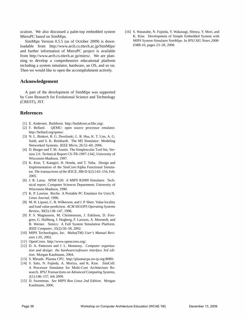
ucation. We also discussed a palm-top embedded systemMieruPC based on SimMips.

SimMips Version 0.5.5 (as of October 2009) is down-loadable from http://www.arch.cs.titech.ac.jp/SimMips/and further information of MieruPC project is availablefrom http://www.arch.cs.titech.ac.jp/mieru/. We are plan-ning to develop a comprehensive educational platformincluding a system simulator, hardware, an OS, and so on.Then we would like to open the accomplishment actively.

Acknowledgement

A part of the development of SimMips was supportedby Core Research for Evolutional Science and Technology(CREST), JST.

References

[1] E. Andersen. Buildroot. http://buildroot.uclibc.org/.[2] F. Bellard. QEMU: open source processor emulator.

http://bellard.org/qemu/.[3] N. L. Binkert, R. G. Dreslinski, L. R. Hsu, K. T. Lim, A. G.

Saidi, and S. K. Reinhardt. The M5 Simulator: ModelingNetworked Systems.IEEE Micro, 26:52–60, 2006.

[4] D. Burger and T. M. Austin. The Simplescalar Tool Set, Ver-sion 2.0. Technical Report CS-TR-1997-1342, University ofWisconsin-Madison, 1997.

[5] K. Kise, T. Katagiri, H. Honda, and T. Yuba. Design andImplementation of the SimCore/Alpha Functional Simula-tor. The transactions of the IEICE, J88-D-I(2):143–154, Feb.2005.

[6] J. R. Larus. SPIM S20: A MIPS R2000 Simulator. Tech-nical report, Computer Sciences Department, University ofWisconsin-Madison, 1990.

[7] K. P. Lawton. Bochs: A Portable PC Emulator for Unix/X.Linux Journal, 1996.

[8] M. H. Lipasti, C. B. Wilkerson, and J. P. Shen. Value localityand load value prediction.ACM SIGOPS Operating SystemsReview, 30(5):138–147, 1996.

[9] P. S. Magnusson, M. Christensson, J. Eskilson, D. Fors-gren, G. Hallberg, J. Hogberg, F. Larsson, A. Moestedt, andB. Werner. Simics: A Full System Simulation Platform.IEEE Computer, 35(2):50–58, 2002.

[10] MIPS Technologies, Inc.Malta(TM) User’s Manual Revi-sion 1.05, 2002.

[11] OpenCores. http://www.opencores.org/.[12] D. A. Patterson and J. L. Hennessy.Computer organiza-

tion and design: the hardware/software interface 3rd edi-tion. Morgan Kaufmann, 2004.

[13] S. Rhoads. Plasma CPU. http://plasmacpu.no-ip.org:8080/.[14] S. Sato, N. Fujieda, A. Moriya, and K. Kise. SimCell:

A Processor Simulator for Multi-Core Architecture Re-search.IPSJ Transactions on Advanced Computing Systems,2(1):146–157, feb 2009.

[15] D. Sweetman.See MIPS Run Linux 2nd Edition. MorganKaufmann, 2006.

[16] S. Watanabe, N. Fujieda, Y. Wakasugi, Shinya, Y. Mori, andK. Kise. Development of Simple Embedded System withMIPS System Simulator SimMips. InIPSJ SIG Notes 2008-EMB-10, pages 23–28, 2008.


WCAE 2009 Workshop on Computer Architecture Education

Documents

Transcript of WCAE 2009 Workshop on Computer Architecture Education