
VibracionConceptos
32
7/17/2019 VibracionConceptos http://slidepdf.com/reader/full/vibracionconceptos 1/32 1 Introduction: Basic Concepts and Terminology 1.1 CONCEPT OF VIBRATION Any repetitive motion is called vibration or oscillation. The motion of a guitar string, motion felt by passengers in an automobile traveling over a bumpy road, swaying of tall buildings due to wind or earthquake, and motion of an airplane in turbulence are typical examples of vibration. The theory of vibration deals with the study of oscillatory motion of bodies and the associated forces. The oscillatory motion shown in Fig. 1.1(a) is called harmonic motion and is denoted as x(t) = X cos ωt (1.1) where X is called the amplitude of motion, ω is the frequency of motion, and t is the time. The motion shown in Fig. 1.1(b) is called periodic motion, and that shown in Fig. 1.1(c) is called nonperiodic or transient motion. The motion indicated in Fig. 1.1(d) is random or long-duration nonperiodic vibration. The phenomenon of vibration involves an alternating interchange of potential energy to kinetic energy and kinetic energy to potential energy. Hence, any vibrat- ing system must have a component that stores potential energy and a component that stores kinetic energy. The components storing potential and kinetic energies are called a spring or elastic element and a mass or inertia element , respectively. The elastic element stores potential energy and gives it up to the inertia element as kinetic energy, and vice versa, in each cycle of motion. The repetitive motion associated with vibra- tion can be explained through the motion of a mass on a smooth surface, as shown in Fig. 1.2. The mass is connected to a linear spring and is assumed to be in equilibrium or rest at position 1. Let the mass m be given an initial displacement to position 2 and released with zero velocity. At position 2, the spring is in a maximum elongated condition, and hence the potential or strain energy of the spring is a maximum and the kinetic energy of the mass will be zero since the initial velocity is assumed to be zero. Because of the tendency of the spring to return to its unstretched condition, there will be a force that causes the mass m to move to the left. The velocity of the mass will gradually increase as it moves from position 2 to position 1. At position 1, the potential energy of the spring is zero because the deformation of the spring is zero. However, the kinetic energy and hence the velocity of the mass will be maximum at position 1 because of conservation of energy (assuming no dissipation of energy due to damping or friction). Since the velocity is maximum at position 1, the mass will 1
-
Upload
yehoyakim-casanova-klein -
Category
Documents
-
view
221 -
download
0
description
vibracion
Transcript of VibracionConceptos

7/17/2019 VibracionConceptos
http://slidepdf.com/reader/full/vibracionconceptos 1/32
1
Introduction: Basic Conceptsand Terminology
1.1 CONCEPT OF VIBRATION
Any repetitive motion is called vibration or oscillation. The motion of a guitar string,
motion felt by passengers in an automobile traveling over a bumpy road, swaying of
tall buildings due to wind or earthquake, and motion of an airplane in turbulence are
typical examples of vibration. The theory of vibration deals with the study of oscillatorymotion of bodies and the associated forces. The oscillatory motion shown in Fig. 1.1(a)
is called harmonic motion and is denoted as
x(t) = X cos ωt (1.1)
where X is called the amplitude of motion, ω is the frequency of motion, and t is the time.
The motion shown in Fig. 1.1(b) is called periodic motion, and that shown in Fig. 1.1(c)
is called nonperiodic or transient motion. The motion indicated in Fig. 1.1(d) is random
or long-duration nonperiodic vibration.
The phenomenon of vibration involves an alternating interchange of potential
energy to kinetic energy and kinetic energy to potential energy. Hence, any vibrat-ing system must have a component that stores potential energy and a component that
stores kinetic energy. The components storing potential and kinetic energies are called
a spring or elastic element and a mass or inertia element , respectively. The elastic
element stores potential energy and gives it up to the inertia element as kinetic energy,
and vice versa, in each cycle of motion. The repetitive motion associated with vibra-
tion can be explained through the motion of a mass on a smooth surface, as shown in
Fig. 1.2. The mass is connected to a linear spring and is assumed to be in equilibrium
or rest at position 1. Let the mass m be given an initial displacement to position 2
and released with zero velocity. At position 2, the spring is in a maximum elongated
condition, and hence the potential or strain energy of the spring is a maximum and
the kinetic energy of the mass will be zero since the initial velocity is assumed to be
zero. Because of the tendency of the spring to return to its unstretched condition, there
will be a force that causes the mass m to move to the left. The velocity of the mass
will gradually increase as it moves from position 2 to position 1. At position 1, the
potential energy of the spring is zero because the deformation of the spring is zero.
However, the kinetic energy and hence the velocity of the mass will be maximum at
position 1 because of conservation of energy (assuming no dissipation of energy due
to damping or friction). Since the velocity is maximum at position 1, the mass will
1

7/17/2019 VibracionConceptos
http://slidepdf.com/reader/full/vibracionconceptos 2/32
2 Introduction: Basic Concepts and Terminology
(c)
0 Time, t
Displacement (or force), x (t )
(a)
X
− X
0
Period,
2pt = w
2pt = w
Period,
Time, t
Displacement (or force), x (t )
Displacement (or force), x (t )
(b)
0 Time, t
Figure 1.1 Types of displacements (or forces): (a) periodic simple harmonic; (b) periodic
nonharmonic; (c) nonperiodic, transient; (d ) nonperiodic, random.

7/17/2019 VibracionConceptos
http://slidepdf.com/reader/full/vibracionconceptos 3/32
1.1 Concept of Vibration 3
Displacement (or force), x (t )
(d )
0 Time, t
Figure 1.1 (continued )
(a)
mk
Position 1 (equilibrium)
x (t )
m
k
Position 2(extreme right)
(b)
m
k
(c)
Position 3(extreme left)
Figure 1.2 Vibratory motion of a spring–mass system: (a) system in equilibrium (spring unde-
formed); (b) system in extreme right position (spring stretched); (c) system in extreme left
position (spring compressed).
continue to move to the left, but against the resisting force due to compression of
the spring. As the mass moves from position 1 to the left, its velocity will gradually
decrease until it reaches a value of zero at position 3. At position 3 the velocity and
hence the kinetic energy of the mass will be zero and the deflection (compression)
and hence the potential energy of the spring will be maximum. Again, because of the

7/17/2019 VibracionConceptos
http://slidepdf.com/reader/full/vibracionconceptos 4/32
4 Introduction: Basic Concepts and Terminology
tendency of the spring to return to its uncompressed condition, there will be a forc
that causes the mass m to move to the right from position 3. The velocity of the mas
will increase gradually as it moves from position 3 to position 1. At position 1, al
of the potential energy of the spring has been converted to the kinetic energy of th
mass, and hence the velocity of the mass will be maximum. Thus, the mass continue
to move to the right against increasing spring resistance until it reaches position 2 with
zero velocity. This completes one cycle of motion of the mass, and the process repeatsthus, the mass will have oscillatory motion.
The initial excitation to a vibrating system can be in the form of initial displace
ment and/or initial velocity of the mass element(s). This amounts to imparting potentia
and/or kinetic energy to the system. The initial excitation sets the system into oscil
latory motion, which can be called free vibration. During free vibration, there wil
be exchange between potential and kinetic energies. If the system is conservative, th
sum of potential energy and kinetic energy will be a constant at any instant. Thus, th
system continues to vibrate forever, at least in theory. In practice, there will be som
damping or friction due to the surrounding medium (e.g., air), which will cause los
of some energy during motion. This causes the total energy of the system to diminish
continuously until it reaches a value of zero, at which point the motion stops. If thsystem is given only an initial excitation, the resulting oscillatory motion eventually
will come to rest for all practical systems, and hence the initial excitation is called
transient excitation and the resulting motion is called transient motion. If the vibratio
of the system is to be maintained in a steady state, an external source must replac
continuously the energy dissipated due to damping.
1.2 IMPORTANCE OF VIBRATION
Any body having mass and elasticity is capable of oscillatory motion. In fact, moshuman activities, including hearing, seeing, talking, walking, and breathing, also involv
oscillatory motion. Hearing involves vibration of the eardrum, seeing is associated wit
the vibratory motion of light waves, talking requires oscillations of the laryng (tongue)
walking involves oscillatory motion of legs and hands, and breathing is based on th
periodic motion of lungs. In engineering, an understanding of the vibratory behavior o
mechanical and structural systems is important for the safe design, construction, an
operation of a variety of machines and structures.
The failure of most mechanical and structural elements and systems can be associ
ated with vibration. For example, the blade and disk failures in steam and gas turbine
and structural failures in aircraft are usually associated with vibration and the resultin
fatigue. Vibration in machines leads to rapid wear of parts such as gears and bearingsloosening of fasteners such as nuts and bolts, poor surface finish during metal cutting
and excessive noise. Excessive vibration in machines causes not only the failure o
components and systems but also annoyance to humans. For example, imbalance in
diesel engines can cause ground waves powerful enough to create a nuisance in urban
areas. Supersonic aircraft create sonic booms that shatter doors and windows. Severa
spectacular failures of bridges, buildings, and dams are associated with wind-induce
vibration, as well as oscillatory ground motion during earthquakes.

7/17/2019 VibracionConceptos
http://slidepdf.com/reader/full/vibracionconceptos 5/32
1.3 Origins and Developments in Mechanics and Vibration 5
In some engineering applications, vibrations serve a useful purpose. For example,
in vibratory conveyors, sieves, hoppers, compactors, dentist drills, electric toothbrushes,
washing machines, clocks, electric massaging units, pile drivers, vibratory testing
of materials, vibratory finishing processes, and materials processing operations such
as casting and forging, vibration is used to improve the efficiency and quality of
the process.
1.3 ORIGINS AND DEVELOPMENTS IN MECHANICS
AND VIBRATION
The earliest human interest in the study of vibration can be traced to the time when the
first musical instruments, probably whistles or drums, were discovered. Since that time,
people have applied ingenuity and critical investigation to study the phenomenon of
vibration and its relation to sound. Although certain very definite rules were observed
in the art of music, even in ancient times, they can hardly be called science. The ancient
Egyptians used advanced engineering concepts such as the use of dovetailed cramps
and dowels in the stone joints of major structures such as the pyramids during the thirdand second millennia b.c.
As far back as 4000 b.c., music was highly developed and well appreciated in
China, India, Japan, and perhaps Egypt [1, 6]. Drawings of stringed instruments such
as harps appeared on the walls of Egyptian tombs as early as 3000 b.c. The British
Museum also has a nanga, a primitive stringed instrument from 155 b.c. The present
system of music is considered to have arisen in ancient Greece.
The scientific method of dealing with nature and the use of logical proofs for
abstract propositions began in the time of Thales of Miletos (640–546 b.c.), who
introduced the term electricity after discovering the electrical properties of yellow
amber. The first person to investigate the scientific basis of musical sounds is considered
to be the Greek mathematician and philosopher Pythagoras (582–507 b.c.). Pythagorasestablished the Pythagorean school, the first institute of higher education and scientific
research. Pythagoras conducted experiments on vibrating strings using an apparatus
called the monochord. Pythagoras found that if two strings of identical properties but
different lengths are subject to the same tension, the shorter string produces a higher
note, and in particular, if the length of the shorter string is one-half that of the longer
string, the shorter string produces a note an octave above the other. The concept of
pitch was known by the time of Pythagoras; however, the relation between the pitch and
the frequency of a sounding string was not known at that time. Only in the sixteenth
century, around the time of Galileo, did the relation between pitch and frequency
become understood [2].
Daedalus is considered to have invented the pendulum in the middle of the secondmillennium b.c. One initial application of the pendulum as a timing device was made
by Aristophanes (450–388 b.c.). Aristotle wrote a book on sound and music around
350 b.c. and documents his observations in statements such as “the voice is sweeter
than the sound of instruments” and “the sound of the flute is sweeter than that of the
lyre.” Aristotle recognized the vectorial character of forces and introduced the concept
of vectorial addition of forces. In addition, he studied the laws of motion, similar to
those of Newton. Aristoxenus, who was a musician and a student of Aristotle, wrote a

7/17/2019 VibracionConceptos
http://slidepdf.com/reader/full/vibracionconceptos 6/32
6 Introduction: Basic Concepts and Terminology
three-volume book called Elements of Harmony. These books are considered the oldes
books available on the subject of music. Alexander of Afrodisias introduced the idea
of potential and kinetic energies and the concept of conservation of energy. In abou
300 b.c., in addition to his contributions to geometry, Euclid gave a brief descriptio
of music in a treatise called Introduction to Harmonics. However, he did not discus
the physical nature of sound in the book. Euclid was distinguished for his teaching
ability, and his greatest work, the Elements, has seen numerous editions and remainone of the most influential books of mathematics of all time. Archimedes (287–21
b.c.) is called by some scholars the father of mathematical physics. He developed th
rules of statics. In his On Floating Bodies, Archimedes developed major rules of flui
pressure on a variety of shapes and on buoyancy.
China experienced many deadly earthquakes in ancient times. Zhang Heng, a histo
rian and astronomer of the second century a.d., invented the world’s first seismograp
to measure earthquakes in a.d. 132 [3]. This seismograph was a bronze vessel in th
form of a wine jar, with an arrangement consisting of pendulums surrounded by
group of eight lever mechanisms pointing in eight directions. Eight dragon figures
with a bronze ball in the mouth of each, were arranged outside the jar. An earthquake
in any direction would tilt the pendulum in that direction, which would cause the releaseof the bronze ball in that direction. This instrument enabled monitoring personnel t
know the direction, time of occurrence, and perhaps, the magnitude of the earthquake
The foundations of modern philosophy and science were laid during the sixteent
century; in fact, the seventeenth century is called the century of genius by many
Galileo (1564–1642) laid the foundations for modern experimental science through hi
measurements on a simple pendulum and vibrating strings. During one of his trips to
the church in Pisa, the swinging movements of a lamp caught Galileo’s attention. He
measured the period of the pendulum movements of the lamp with his pulse and wa
amazed to find that the time period was not influenced by the amplitude of swings
Subsequently, Galileo conducted more experiments on the simple pendulum and pub
lished his findings in Discourses Concerning Two New Sciences in 1638. In this workhe discussed the relationship between the length and the frequency of vibration of
simple pendulum, as well as the idea of sympathetic vibrations or resonance [4].
Although the writings of Galileo indicate that he understood the interdependenc
of the parameters—length, tension, density and frequency of transverse vibration—o
a string, they did not offer an analytical treatment of the problem. Marinus Mersenn
(1588– 1648), a mathematician and theologian from France, described the correct behav
ior of the vibration of strings in 1636 in his book Harmonicorum Liber . For the firs
time, by knowing (measuring) the frequency of vibration of a long string, Mersenn
was able to predict the frequency of vibration of a shorter string having the same den
sity and tension. He is considered to be the first person to discover the laws of vibratin
strings. The truth was that Galileo was the first person to conduct experimental studieon vibrating strings; however, publication of his work was prohibited until 1638, b
order of the Inquisitor of Rome. Although Galileo studied the pendulum extensivel
and discussed the isochronism of the pendulum, Christian Huygens (1629–1695) wa
the person who developed the pendulum clock, the first accurate device develope
for measuring time. He observed deviation from isochronism due to the nonlinear
ity of the pendulum, and investigated various designs to improve the accuracy of th
pendulum clock.

7/17/2019 VibracionConceptos
http://slidepdf.com/reader/full/vibracionconceptos 7/32
1.3 Origins and Developments in Mechanics and Vibration 7
The works of Galileo contributed to a substantially increased level of experimen-
tal work among many scientists and paved the way to the establishment of several
professional organizations, such as the Academia Naturae in Naples in 1560, Academia
dei Lincei in Rome in 1606, Royal Society in London in 1662, the French Academy
of Sciences in 1766, and the Berlin Academy of Science in 1770.
The relation between the pitch and frequency of vibration of a taut string was
investigated further by Robert Hooke (1635–1703) and Joseph Sauveur (1653–1716).The phenomenon of mode shapes during the vibration of stretched strings, involving no
motion at certain points and violent motion at intermediate points, was observed inde-
pendently by Sauveur in France (1653–1716) and John Wallis in England (1616–1703).
Sauveur called points with no motion nodes and points with violent motion, loops. Also,
he observed that vibrations involving nodes and loops had higher frequencies than those
involving no nodes. After observing that the values of the higher frequencies were inte-
gral multiples of the frequency of simple vibration with no nodes, Sauveur termed the
frequency of simple vibration the fundamental frequency and the higher frequencies,
the harmonics. In addition, he found that the vibration of a stretched string can con-
tain several harmonics simultaneously. The phenomenon of beats was also observed
by Sauveur when two organ pipes, having slightly different pitches, were soundedtogether. He also tried to compute the frequency of vibration of a taut string from the
measured sag of its middle point. Sauveur introduced the word acoustics for the first
time for the science of sound [7].
Isaac Newton (1642–1727) studied at Trinity College, Cambridge and later became
professor of mathematics at Cambridge and president of the Royal Society of London.
In 1687 he published the most admired scientific treatise of all time, Philosophia Natu-
ralis Principia Mathematica. Although the laws of motion were already known in one
form or other, the development of differential calculus by Newton and Leibnitz made
the laws applicable to a variety of problems in mechanics and physics. Leonhard Euler
(1707–1783) laid the groundwork for the calculus of variations. He popularized the
use of free-body diagrams in mechanics and introduced several notations, includinge = 2.71828 . . ., f (x),
, and i = √ −1. In fact, many people believe that the current
techniques of formulating and solving mechanics problems are due more to Euler than
to any other person in the history of mechanics. Using the concept of inertia force,
Jean D’Alembert (1717–1783) reduced the problem of dynamics to a problem in stat-
ics. Joseph Lagrange (1736–1813) developed the variational principles for deriving the
equations of motion and introduced the concept of generalized coordinates. He intro-
duced Lagrange equations as a powerful tool for formulating the equations of motion
for lumped-parameter systems. Charles Coulomb (1736–1806) studied the torsional
oscillations both theoretically and experimentally. In addition, he derived the relation
between electric force and charge.
Claude Louis Marie Henri Navier (1785–1836) presented a rigorous theory forthe bending of plates. In addition, he considered the vibration of solids and presented
the continuum theory of elasticity. In 1882, Augustin Louis Cauchy (1789–1857) pre-
sented a formulation for the mathematical theory of continuum mechanics. William
Hamilton (1805– 1865) extended the formulation of Lagrange for dynamics prob-
lems and presented a powerful method (Hamilton’s principle) for the derivation of
equations of motion of continuous systems. Heinrich Hertz (1857–1894) introduced the
terms holonomic and nonholonomic into dynamics around 1894. Jules Henri Poincare

7/17/2019 VibracionConceptos
http://slidepdf.com/reader/full/vibracionconceptos 8/32
8 Introduction: Basic Concepts and Terminology
(1854–1912) made many contributions to pure and applied mathematics, particularl
to celestial mechanics and electrodynamics. His work on nonlinear vibrations in term
of the classification of singular points of nonlinear autonomous systems is notable.
1.4 HISTORY OF VIBRATION OF CONTINUOUS SYSTEMS
The precise treatment of the vibration of continuous systems can be associated witthe discovery of the basic law of elasticity by Hooke, the second law of motion by
Newton, and the principles of differential calculus by Leibnitz. Newton’s second law
of motion is used routinely in modern books on vibrations to derive the equations o
motion of a vibrating body.
Strings A theoretical (dynamical) solution of the problem of the vibrating string wa
found in 1713 by the English mathematician Brook Taylor (1685–1731), who also pre
sented the famous Taylor theorem on infinite series. He applied the fluxion approach
similar to the differential calculus approach developed by Newton and Newton’s sec
ond law of motion, to an element of a continuous string and found the true valu
of the first natural frequency of the string. This value was found to agree with theexperimental values observed by Galileo and Mersenne. The procedure adopted b
Taylor was perfected through the introduction of partial derivatives in the equation
of motion by Daniel Bernoulli, Jean D’Alembert, and Leonhard Euler. The fluxion
method proved too clumsy for use with more complex vibration analysis problems
With the controversy between Newton and Leibnitz as to the origin of differential cal
culus, patriotic Englishmen stuck to the cumbersome fluxions while other investigator
in Europe followed the simpler notation afforded by the approach of Leibnitz.
In 1747, D’Alembert derived the partial differential equation, later referred to as th
wave equation, and found the wave travel solution. Although D’Alembert was assiste
by Daniel Bernoulli and Leonhard Euler in this work, he did not give them credit. Wit
all three claiming credit for the work, the specific contribution of each has remainedcontroversial.
The possibility of a string vibrating with several of its harmonics present at the sam
time (with displacement of any point at any instant being equal to the algebraic sum o
displacements for each harmonic) was observed by Bernoulli in 1747 and proved by
Euler in 1753. This was established through the dynamic equations of Daniel Bernoul
in his memoir, published by the Berlin Academy in 1755. This characteristic wa
referred to as the principle of the coexistence of small oscillations, which is the same a
the principle of superposition in today’s terminology. This principle proved to be ver
valuable in the development of the theory of vibrations and led to the possibility o
expressing any arbitrary function (i.e., any initial shape of the string) using an infinite
series of sine and cosine terms. Because of this implication, D’Alembert and Euledoubted the validity of this principle. However, the validity of this type of expansion
was proved by Fourier (1768–1830) in his Analytical Theory of Heat in 1822.
It is clear that Bernoulli and Euler are to be credited as the originators of th
modal analysis procedure. They should also be considered the originators of the Fourie
expansion method. However, as with many discoveries in the history of science, the
persons credited with the achievement may not deserve it completely. It is often th
person who publishes at the right time who gets the credit.

7/17/2019 VibracionConceptos
http://slidepdf.com/reader/full/vibracionconceptos 9/32
1.4 History of Vibration of Continuous Systems 9
The analytical solution of the vibrating string was presented by Joseph Lagrange in
his memoir published by the Turin Academy in 1759. In his study, Lagrange assumed
that the string was made up of a finite number of equally spaced identical mass particles,
and he established the existence of a number of independent frequencies equal to the
number of mass particles. When the number of particles was allowed to be infinite,
the resulting frequencies were found to be the same as the harmonic frequencies of
the stretched string. The method of setting up the differential equation of motion of astring (called the wave equation), presented in most modern books on vibration theory,
was developed by D’Alembert and described in his memoir published by the Berlin
Academy in 1750.
Bars Chladni in 1787, and Biot in 1816, conducted experiments on the longitudinal
vibration of rods. In 1824, Navier, presented an analytical equation and its solution for
the longitudinal vibration of rods.
Shafts Charles Coulomb did both theoretical and experimental studies in 1784 on the
torsional oscillations of a metal cylinder suspended by a wire [5]. By assuming that the
resulting torque of the twisted wire is proportional to the angle of twist, he derived an
equation of motion for the torsional vibration of a suspended cylinder. By integrating
the equation of motion, he found that the period of oscillation is independent of the
angle of twist. The derivation of the equation of motion for the torsional vibration
of a continuous shaft was attempted by Caughy in an approximate manner in 1827
and given correctly by Poisson in 1829. In fact, Saint-Venant deserves the credit for
deriving the torsional wave equation and finding its solution in 1849.
Beams The equation of motion for the transverse vibration of thin beams was derived
by Daniel Bernoulli in 1735, and the first solutions of the equation for various support
conditions were given by Euler in 1744. Their approach has become known as the
Euler– Bernoulli or thin beam theory. Rayleigh presented a beam theory by including
the effect of rotary inertia. In 1921, Stephen Timoshenko presented an improved theoryof beam vibration, which has become known as the Timoshenko or thick beam theory,
by considering the effects of rotary inertia and shear deformation.
Membranes In 1766, Euler, derived equations for the vibration of rectangular mem-
branes which were correct only for the uniform tension case. He considered the
rectangular membrane instead of the more obvious circular membrane in a drumhead,
because he pictured a rectangular membrane as a superposition of two sets of strings
laid in perpendicular directions. The correct equations for the vibration of rectangular
and circular membranes were derived by Poisson in 1828. Although a solution corre-
sponding to axisymmetric vibration of a circular membrane was given by Poisson, a
nonaxisymmetric solution was presented by Pagani in 1829.
Plates The vibration of plates was also being studied by several investigators at this
time. Based on the success achieved by Euler in studying the vibration of a rectangular
membrane as a superposition of strings, Euler’s student James Bernoulli, the grand-
nephew of the famous mathematician Daniel Bernoulli, attempted in 1788 to derive
an equation for the vibration of a rectangular plate as a gridwork of beams. However,
the resulting equation was not correct. As the torsional resistance of the plate was not

7/17/2019 VibracionConceptos
http://slidepdf.com/reader/full/vibracionconceptos 10/32
10 Introduction: Basic Concepts and Terminology
considered in his equation of motion, only a resemblance, not the real agreement, wa
noted between the theoretical and experimental results.
The method of placing sand on a vibrating plate to find its mode shapes and to
observe the various intricate modal patterns was developed by the German scientis
Chladni in 1802. In his experiments, Chladni distributed sand evenly on horizonta
plates. During vibration, he observed regular patterns of modes because of the accu
mulation of sand along the nodal lines that had no vertical displacement. NapoleoBonaparte, who was a trained military engineer, was present when Chladni gave
demonstration of his experiments on plates at the French Academy in 1809. Napoleo
was so impressed by Chladni’s demonstration that he gave a sum of 3000 francs to th
French Academy to be presented to the first person to give a satisfactory mathemati
cal theory of the vibration of plates. When the competition was announced, only on
person, Sophie Germain, entered the contest by the closing date of October 1811 [8]
However, an error in the derivation of Germain’s differential equation was noted b
one of the judges, Lagrange. In fact, Lagrange derived the correct form of the differ
ential equation of plates in 1811. When the academy opened the competition again
with a new closing date of October 1813, Germain entered the competition again with
a correct form of the differential equation of plates. Since the judges were not satisfieddue to the lack of physical justification of the assumptions she made in deriving th
equation, she was not awarded the prize. The academy opened the competition agai
with a new closing date of October 1815. Again, Germain entered the contest. Thi
time she was awarded the prize, although the judges were not completely satisfied with
her theory. It was found later that her differential equation for the vibration of plate
was correct but the boundary conditions she presented were wrong. In fact, Kirchhoff
in 1850, presented the correct boundary conditions for the vibration of plates as wel
as the correct solution for a vibrating circular plate.
The great engineer and bridge designer Navier (1785–1836) can be considere
the originator of the modern theory of elasticity. He derived the correct differentia
equation for rectangular plates with flexural resistance. He presented an exact methothat transforms the differential equation into an algebraic equation for the solution o
plate and other boundary value problems using trigonometric series. In 1829, Poisson
extended Navier’s method for the lateral vibration of circular plates.
Kirchhoff (1824–1887) who included the effects of both bending and stretching in
his theory of plates published in his book Lectures on Mathematical Physics, is con
sidered the founder of the extended plate theory. Kirchhoff’s book was translated int
French by Clebsch with numerous valuable comments by Saint-Venant. Love extende
Kirchhoff’s approach to thick plates. In 1915, Timoshenko presented a solution fo
circular plates with large deflections. Foppl considered the nonlinear theory of plate
in 1907; however, the final form of the differential equation for the large deflectio
of plates was developed by von Karman in 1910. A more rigorous plate theory thaconsiders the effects of transverse shear forces was presented by Reissner. A plate the
ory that includes the effects of both rotatory inertia and transverse shear deformation
similar to the Timoshenko beam theory, was presented by Mindlin in 1951.
Shells The derivation of an equation for the vibration of shells was attempted b
Sophie Germain, who in 1821 published a simplified equation, with errors, for the
vibration of a cylindrical shell. She assumed that the in-plane displacement of th

7/17/2019 VibracionConceptos
http://slidepdf.com/reader/full/vibracionconceptos 11/32
1.5 Discrete and Continuous Systems 11
neutral surface of a cylindrical shell was negligible. Her equation can be reduced to
the correct form for a rectangular plate but not for a ring. The correct equation for the
vibration of a ring had been given by Euler in 1766.
Aron, in 1874, derived the general shell equations in curvilinear coordinates, which
were shown to reduce to the plate equation when curvatures were set to zero. The
equations were complicated because no simplifying assumptions were made. Lord
Rayleigh proposed different simplifications for the vibration of shells in 1882 andconsidered the neutral surface of the shell either extensional or inextensional. Love, in
1888, derived the equations for the vibration of shells by using simplifying assumptions
similar to those of beams and plates for both in-plane and transverse motions. Love’s
equations can be considered to be most general in unifying the theory of vibration
of continuous structures whose thickness is small compared to other dimensions. The
vibration of shells, with a consideration of rotatory inertia and shear deformation, was
presented by Soedel in 1982.
Approximate Methods Lord Rayleigh published his book on the theory of sound in
1877; it is still considered a classic on the subject of sound and vibration. Notable among
the many contributions of Rayleigh is the method of finding the fundamental frequency
of vibration of a conservative system by making use of the principle of conservation
of energy—now known as Rayleigh’s method . Ritz (1878–1909) extended Rayleigh’s
method for finding approximate solutions of boundary value problems. The method,
which became known as the Rayleigh – Ritz method , can be considered to be a varia-
tional approach. Galerkin (1871–1945) developed a procedure that can be considered
a weighted residual method for the approximate solution of boundary value problems.
Until about 40 years ago, vibration analyses of even the most complex engineer-
ing systems were conducted using simple approximate analytical methods. Continuous
systems were modeled using only a few degrees of freedom. The advent of high-
speed digital computers in the 1950s permitted the use of more degrees of freedom
in modeling engineering systems for the purpose of vibration analysis. Simultaneous
development of the finite element method in the 1960s made it possible to consider
thousands of degrees of freedom to approximate practical problems in a wide spectrum
of areas, including machine design, structural design, vehicle dynamics, and engineering
mechanics. Notable contributions to the theory of the vibration of continuous systems
are summarized in Table 1.1.
1.5 DISCRETE AND CONTINUOUS SYSTEMS
The degrees of freedom of a system are defined by the minimum number of independent
coordinates necessary to describe the positions of all parts of the system at any instant
of time. For example, the spring–mass system shown in Fig. 1.2 is a single-degree-of-freedom system since a single coordinate, x(t), is sufficient to describe the position of
the mass from its equilibrium position at any instant of time. Similarly, the simple pen-
dulum shown in Fig. 1.3 also denotes a single-degree-of-freedom system. The reason
is that the position of a simple pendulum during motion can be described by using a
single angular coordinate, θ . Although the position of a simple pendulum can be stated
in terms of the Cartesian coordinates x and y , the two coordinates x and y are not inde-
pendent; they are related to one another by the constraint x2 + y2 = l 2, where l is the

7/17/2019 VibracionConceptos
http://slidepdf.com/reader/full/vibracionconceptos 12/32
12 Introduction: Basic Concepts and Terminology
Table 1.1 Notable Contributions to the Theory of Vibration of Continuous Systems
Period Scientist Contribution
582–507 b.c. Pythagoras Established the first school of higher education
and scientific research. Conducted
experiments on vibrating strings. Invented
the monochord.
384–322 b.c. Aristotle Wrote a book on acoustics. Studied laws of
motion (similar to those of Newton).
Introduced vectorial addition of forces.
Third century
b.c.
Alexander of
Afrodisias
Kinetic and potential energies. Idea of
conservation of energy.
325–265 b.c. Euclid Prominent mathematician. Published a treatise
called Introduction to Harmonics.
a.d.
1564–1642 Galileo Galilei Experiments on pendulum and vibration of
strings. Wrote the first treatise on modern
dynamics.1642–1727 Isaac Newton Laws of motion. Differential calculus.
Published the famous Principia
Mathematica.
1653–1716 Joseph Sauveur Introduced the term acoustics. Investigated
harmonics in vibration.
1685–1731 Brook Taylor Theoretical solution of vibrating strings.
Taylor’s theorem.
1700–1782 Daniel Bernoulli Principle of angular momentum. Principle of
superposition.
1707–1783 Leonhard Euler Principle of superposition. Beam theory.
Vibration of membranes. Introduced severalmathematical symbols.
1717–1783 Jean D’Alembert Dynamic equilibrium of bodies in motion.
Inertia force. Wave equation.
1736–1813 Joseph Louis
Lagrange
Analytical solution of vibrating strings.
Lagrange’s equations. Variational calculus.
Introduced the term generalized coordinates.
1736–1806 Charles Coulomb Torsional vibration studies.
1756–1827 E. F. F. Chladni Experimental observation of mode shapes of
plates.
1776–1831 Sophie Germain Vibration of plates.
1785–1836 Claude Louis
Marie Henri
Navier
Bending vibration of plates. Vibration of solids.
Originator of modern theory of elasticity.
1797 – 1872 Jean Marie
Duhamel
Studied partial differential equations applied to
vibrating strings and vibration of air in
pipes. Duhamel’s integral.
1805 –1865 William
Hamilton
Principle of least action. Hamilton’s principle.

7/17/2019 VibracionConceptos
http://slidepdf.com/reader/full/vibracionconceptos 13/32
1.5 Discrete and Continuous Systems 13
Table 1.1 (continued )
Period Scientist Contribution
1824–1887 Gustav Robert
Kirchhoff
Presented extended theory of plates.
Kirchhoff’s laws of electrical circuits.
1842–1919 John William
Strutt (LordRayleigh)
Energy method. Effect of rotatory inertia. Shell
equations.
1874 H. Aron Shell equations in curvilinear coordinates.
1888 A. E. H. Love Classical theory of thin shells.
1871–1945 Boris Grigorevich
Galerkin
Approximate solution of boundary value
problems with application to elasticity and
vibration.
1878–1909 Walter Ritz Extended Rayleigh’s energy method for
approximate solution of boundary value
problems.
1956 Turner, Clough,
Martin, andTopp
Finite element method.
x
y
Datum
O
l
q
Figure 1.3 Simple pendulum.
constant length of the pendulum. Thus, the pendulum is a single-degree-of-freedom sys-
tem. The mass–spring– damper systems shown in Fig. 1.4(a) and (b) denote two- and
three-degree-of-freedom systems, respectively, since they have, two and three masses
that change their positions with time during vibration. Thus, a multidegree-of-freedom
system can be considered to be a system consisting of point masses separated by springs
and dampers. The parameters of the system are discrete sets of finite numbers. These
systems are also called lumped-parameter , discrete, or finite-dimensional systems.

7/17/2019 VibracionConceptos
http://slidepdf.com/reader/full/vibracionconceptos 14/32
14 Introduction: Basic Concepts and Terminology
k 1 k 2
x 1 x 2
m1 m2
(a)
(b)
k 2 k 3 k 4k 1
x 1 x 2
m1
x 3
m3m2
Figure 1.4 (a) Two- and (b) three-degree-of-freedom systems.
On the other hand, in a continuous system, the mass, elasticity (or flexibility), an
damping are distributed throughout the system. During vibration, each of the infinit
number of point masses moves relative to each other point mass in a continuous fash
ion. These systems are also known as distributed, continuous, or infinite-dimensiona
systems. A simple example of a continuous system is the cantilever beam shown in
Fig. 1.5. The beam has an infinite number of mass points, and hence an infinite num
ber of coordinates are required to specify its deflected shape. The infinite number o
coordinates, in fact, define the elastic deflection curve of the beam. Thus, the cantileve
beam is considered to be a system with an infinite number of degrees of freedom. Mos
mechanical and structural systems have members with continuous elasticity and mas
distribution and hence have infinite degrees of freedom.The choice of modeling a given system as discrete or continuous depends on the
purpose of the analysis and the expected accuracy of the results. The motion of an n
degree-of-freedom system is governed by a system of n coupled second-order ordinar
differential equations. For a continuous system, the governing equation of motion i
in the form of a partial differential equation. Since the solution of a set of ordinar
differential equations is simple, it is relatively easy to find the response of a discret
system that is experiencing a specified excitation. On the other hand, solution of
partial differential equation is more involved, and closed-form solutions are availabl
for only a few continuous systems that have a simple geometry and simple, boundary
conditions and excitations. However, the closed-form solutions that are available wil
often provide insight into the behavior of more complex systems for which closed-formsolutions cannot be found.
For an n -degree-of-freedom system, there will be, at most, n distinct natural fre
quencies of vibration with a mode shape corresponding to each natural frequency. A
continuous system, on the other hand, will have an infinite number of natural fre
quencies, with one mode shape corresponding to each natural frequency. A continuou
system can be approximated as a discrete system, and its solution can be obtaine
in a simpler manner. For example, the cantilever beam shown in Fig. 1.5(a) can b
7/17/2019 VibracionConceptos
http://slidepdf.com/reader/full/vibracionconceptos 15/32
1.6 Vibration Problems 15
k =
x (t )
m
3 EI
l3
l
E , I
x 1
x 2
x 3 x 4
x 5
(a)
(b)
k 1
x 1(t )
m1
k 2
x 2(t )
m2
(c)
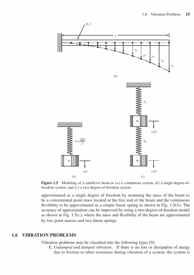
Figure 1.5 Modeling of a cantilever beam as (a) a continuous system, (b) a single-degree-of-
freedom system, and (c) a two-degree-of-freedom system.
approximated as a single degree of freedom by assuming the mass of the beam to
be a concentrated point mass located at the free end of the beam and the continuous
flexibility to be approximated as a simple linear spring as shown in Fig. 1.5(b). The
accuracy of approximation can be improved by using a two-degree-of-freedom model
as shown in Fig. 1.5(c), where the mass and flexibility of the beam are approximated
by two point masses and two linear springs.
1.6 VIBRATION PROBLEMS
Vibration problems may be classified into the following types [9]:1. Undamped and damped vibration . If there is no loss or dissipation of energy
due to friction or other resistance during vibration of a system, the system is

7/17/2019 VibracionConceptos
http://slidepdf.com/reader/full/vibracionconceptos 16/32
16 Introduction: Basic Concepts and Terminology
said to be undamped . If there is energy loss due to the presence of damping, th
system is called damped . Although system analysis is simpler when neglectin
damping, a consideration of damping becomes extremely important if the system
operates near resonance.
2. Free and forced vibration. If a system vibrates due to an initial disturbanc
(with no external force applied after time zero), the system is said to undergo
free vibration. On the other hand, if the system vibrates due to the applicationof an external force, the system is said to be under forced vibration.
3. Linear and nonlinear vibration. If all the basic components of a vibratin
system (i.e., the mass, the spring, and the damper) behave linearly, the resultin
vibration is called linear vibration. However, if any of the basic components o
a vibrating system behave nonlinearly, the resulting vibration is called nonlinea
vibration. The equation of motion governing linear vibration will be a linea
differential equation, whereas the equation governing nonlinear vibration wil
be a nonlinear differential equation. Most vibratory systems behave nonlinearl
as the amplitudes of vibration increase to large values.
1.7 VIBRATION ANALYSIS
A vibratory system is a dynamic system for which the response (output) depend
on the excitations (inputs) and the characteristics of the system (e.g., mass, stiffness
and damping) as indicated in Fig. 1.6. The excitation and response of the system ar
both time dependent. Vibration analysis of a given system involves determination o
the response for the excitation specified. The analysis usually involves mathematica
modeling, derivation of the governing equations of motion, solution of the equation
of motion, and interpretation of the response results.
The purpose of mathematical modeling is to represent all the important charac
teristics of a system for the purpose of deriving mathematical equations that goverthe behavior of the system. The mathematical model is usually selected to includ
enough details to describe the system in terms of equations that are not too complex
The mathematical model may be linear or nonlinear, depending on the nature of the
system characteristics. Although linear models permit quick solutions and are simple t
deal with, nonlinear models sometimes reveal certain important behavior of the system
which cannot be predicted using linear models. Thus, a great deal of engineering judg
ment is required to develop a suitable mathematical model of a vibrating system. If th
mathematical model of the system is linear, the principle of superposition can be used
This means that if the responses of the system under individual excitations f 1(t) an
f 2(t) are denoted as x1(t ) and x2(t ), respectively, the response of the system would b
Excitation, f (t )(input)
Response, x (t )
(output)
System(mass, stiffness,and damping)
Figure 1.6 Input–output relationship of a vibratory system.

7/17/2019 VibracionConceptos
http://slidepdf.com/reader/full/vibracionconceptos 17/32
1.8 Excitations 17
x(t) = c1x1(t) + c2x2(t) when subjected to the excitation f (t ) = c1f 1(t) + c2f 2(t ),
where c1 and c2 are constants.
Once the mathematical model is selected, the principles of dynamics are used
to derive the equations of motion of the vibrating system. For this, the free-body
diagrams of the masses, indicating all externally applied forces (excitations), reaction
forces, and inertia forces, can be used. Several approaches, such as D’Alembert’s
principle, Newton’s second law of motion, and Hamilton’s principle, can be used toderive the equations of motion of the system. The equations of motion can be solved
using a variety of techniques to obtain analytical (closed-form) or numerical solutions,
depending on the complexity of the equations involved. The solution of the equations of
motion provides the displacement, velocity, and acceleration responses of the system.
The responses and the results of analysis need to be interpreted with a clear view of
the purpose of the analysis and the possible design implications.
1.8 EXCITATIONS
Several types of excitations or loads can act on a vibrating system. As stated earlier,the excitation may be in the form of initial displacements and initial velocities that are
produced by imparting potential energy and kinetic energy to the system, respectively.
The response of the system due to initial excitations is called free vibration. For real-
life systems, the vibration caused by initial excitations diminishes to zero eventually
and the initial excitations are known as transient excitations.
In addition to the initial excitations, a vibrating system may be subjected to a
large variety of external forces. The origin of these forces may be environmental,
machine induced, vehicle induced, or blast induced. Typical examples of environmen-
tally induced dynamic forces include wind loads, wave loads, and earthquake loads.
Machine-induced loads are due primarily to imbalance in reciprocating and rotating
machines, engines, and turbines, and are usually periodic in nature. Vehicle-induced loads are those induced on highway and railway bridges from speeding trucks and
trains crossing them. In some cases, dynamic forces are induced on bodies and equip-
ment located inside vehicles due to the motion of the vehicles. For example, sensitive
navigational equipment mounted inside the cockpit of an aircraft may be subjected
to dynamic loads induced by takeoff, landing, or in-flight turbulence. Blast-induced
loads include those generated by explosive devices during blast operations, accidental
chemical explosions, or terrorist bombings.
The nature of some of the dynamic loads originating from different sources is
shown in Fig. 1.1. In the case of rotating machines with imbalance, the induced loads
will be harmonic, as shown in Fig. 1.1(a). In other types of machines, the loads induced
due to the unbalance will be periodic, as shown in Fig. 1.1(b). A blast load acting on avibrating structure is usually in the form of an overpressure, as shown in Fig. 1.1(c). The
blast overpressure will cause severe damage to structures located close to the explosion.
On the other hand, a large explosion due to underground detonation may even affect
structures located far away from the explosion. Earthquake-, wave-, and wind-, gust-,
or turbulence-, induced loads will be random in nature, as indicated in Fig. 1.1(d ).
It can be seen that harmonic force is the simplest type of force to which a vibrating
system can be subjected. The harmonic force also plays a very important role in the
7/17/2019 VibracionConceptos
http://slidepdf.com/reader/full/vibracionconceptos 18/32
18 Introduction: Basic Concepts and Terminology
study of vibrations. For example, any periodic force can be represented as an infinit
sum of harmonic forces using Fourier series. In addition, any nonperiodic force can b
represented (by considering its period to be approaching infinity) in terms of harmoni
forces using the Fourier integral. Because of their importance in vibration analysis,
detailed discussion of harmonic functions is given in the following section.
1.9 HARMONIC FUNCTIONS
In most practical applications, harmonic time dependence is considered to be same a
sinusoidal vibration. For example, the harmonic variations of alternating current and
electromagnetic waves are represented by sinusoidal functions. As an application in
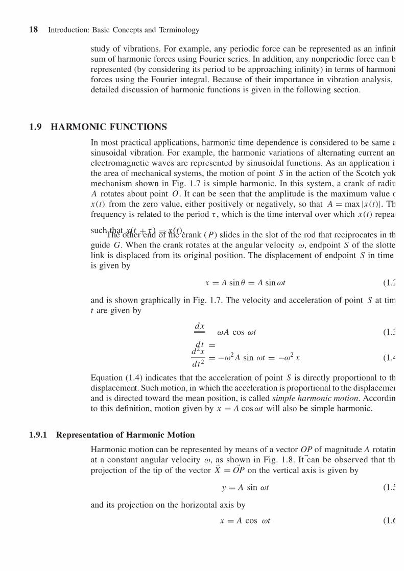
the area of mechanical systems, the motion of point S in the action of the Scotch yok
mechanism shown in Fig. 1.7 is simple harmonic. In this system, a crank of radiu
A rotates about point O. It can be seen that the amplitude is the maximum value o
x(t) from the zero value, either positively or negatively, so that A = max |x(t)|. Th
frequency is related to the period τ , which is the time interval over which x(t) repeat
such that x(t + τ ) = x(t).The other end of the crank (P ) slides in the slot of the rod that reciprocates in th
guide G. When the crank rotates at the angular velocity ω, endpoint S of the slotte
link is displaced from its original position. The displacement of endpoint S in time
is given by
x = A sin θ = A sin ωt (1.2
and is shown graphically in Fig. 1.7. The velocity and acceleration of point S at tim
t are given by
d x
d t = ωA cos ωt (1.3
d 2x
d t 2 = −ω2A sin ωt = −ω2 x (1.4
Equation (1.4) indicates that the acceleration of point S is directly proportional to th
displacement. Such motion, in which the acceleration is proportional to the displacemen
and is directed toward the mean position, is called simple harmonic motion. Accordin
to this definition, motion given by x = A cos ωt will also be simple harmonic.
1.9.1 Representation of Harmonic Motion
Harmonic motion can be represented by means of a vector OP of magnitude A rotatin
at a constant angular velocity ω, as shown in Fig. 1.8. It can be observed that th
projection of the tip of the vector X = OP on the vertical axis is given by
y = A sin ωt (1.5
and its projection on the horizontal axis by
x = A cos ωt (1.6

7/17/2019 VibracionConceptos
http://slidepdf.com/reader/full/vibracionconceptos 19/32
1.9 Harmonic Functions 19
Slotted link
Guide, G
O
A
q = wt
q = wt
4p
3p
2p
p x = A sin wt
x
− A OP
S
A x (t )
Figure 1.7 Simple harmonic motion produced by a Scotch yoke mechanism.
Equations (1.5) and (1.6) both represent simple harmonic motion. In the vectorial
method of representing harmonic motion, two equations, Eqs. (1.5) and (1.6), are
required to describe the vertical and horizontal components. Harmonic motion can
be represented more conveniently using complex numbers. Any vector X can be rep-
resented as a complex number in the xy plane as
X = a + ib (1.7)
where i = √ −1 and a and b denote the x and y components of X, respectively, and
can be considered as the real and imaginary parts of the vector X. The vector X can
also be expressed as
X = A (cos θ + i sin θ ) (1.8)

7/17/2019 VibracionConceptos
http://slidepdf.com/reader/full/vibracionconceptos 20/32
20 Introduction: Basic Concepts and Terminology
Onecycle
Onecycle
− A cos q
x
x
A sin q A
− A
y y
P
OO
p
p
2p
3p
4p
q = wt
q = wt
q = wt
2p 3p 4p
O− A A
P
AP
Figure 1.8 Harmonic motion: projection of a rotating vector.
where
A = (a 2 + b2)1/2 (1.9
denotes the modulus or magnitude of the vector X and
θ = tan−1 b
a(1.10
indicates the argument or the angle between the vector and the x axis. Noting that
cos θ + i sin θ = e iθ (1.11
Eq. (1.8) can be expressed as
X
= A(cos θ
+ i sin θ )
= Aeiθ (1.12
Thus, the rotating vector X of Fig. 1.8 can be written, using complex number repre
sentation, as
X = Ae iωt (1.13
where ω denotes the circular frequency (rad/sec) of rotation of the vector X i
the counterclockwise direction. The harmonic motion given by Eq. (1.13) can b

7/17/2019 VibracionConceptos
http://slidepdf.com/reader/full/vibracionconceptos 21/32
1.9 Harmonic Functions 21
differentiated with respect to time as
d Xd t
= d
d t (Aeiωt ) = iωAeiωt = i ω X (1.14)
d 2 Xdt 2
= d
d t (iωAeiωt ) = −ω2Aeiωt = −ω2 X (1.15)
Thus, if X denotes harmonic motion, the displacement, velocity, and acceleration can
be expressed as
x(t) = displacement = Re[Aeiωt ] = A cos ωt (1.16)
x(t) = velocity = Re[iωAeiωt ] = −ωA sin ωt = ωA cos(ωt + 90◦
) (1.17)
x(t) = acceleration = Re[−ω2Aeiωt ] = −ω2A cos ωt = ω2A cos(ωt + 180◦
) (1.18)
where Re denotes the real part, or alternatively as
x(t)
= displacement
= Im[Aeiωt ]
= A sin ωt (1.19)
x(t) = velocity = Im[iωAeiωt ] = ωA cos ωt = ωA sin(ωt + 90◦
) (1.20)
x(t) = acceleration = Im[−ω2Aeiωt ] = −ω2A sin ωt = ω2A sin(ωt + 180◦
) (1.21)
where Im denotes the imaginary part. Eqs. (1.16)–(1.21) are shown as rotating vectors
in Fig. 1.9. It can be seen that the acceleration vector leads the velocity vector by 90◦,
and the velocity vector leads the displacement vector by 90◦.
1.9.2 Definitions and Terminology
Several definitions and terminology are used to describe harmonic motion and other
periodic functions. The motion of a vibrating body from its undisturbed or equilibriumposition to its extreme position in one direction, then to the equilibrium position, then
p/2
p/2
Im
Re O
x
x
wt p 2p
wt
X = iX w
X
X = − X w2
·
x, x, x · ·· x, x, x · ··
x ··
→ →
→ →
→
w
Figure 1.9 Displacement (x), velocity (x), and acceleration (x) as rotating vectors.

7/17/2019 VibracionConceptos
http://slidepdf.com/reader/full/vibracionconceptos 22/32
22 Introduction: Basic Concepts and Terminology
to its extreme position in the other direction, and then back to the equilibrium position
is called a cycle of vibration. One rotation or an angular displacement of 2π radians o
pin P in the Scotch yoke mechanism of Fig. 1.7 or the vector OP in Fig. 1.8 represent
a cycle.
The amplitude of vibration denotes the maximum displacement of a vibrating bod
from its equilibrium position. The amplitude of vibration is shown as A in Figs. 1.
and 1.8. The period of oscillation represents the time taken by the vibrating body tocomplete one cycle of motion. The period of oscillation is also known as the tim
period and is denoted by τ . In Fig. 1.8, the time period is equal to the time taken by
the vector OP to rotate through an angle of 2π . This yields
τ = 2π
ω(1.22
where ω is called the circular frequency. The frequency of oscillation or linear fre
quency (or simply the frequency) indicates the number of cycles per unit time. Th
frequency can be represented as
f
= 1
τ = ω
2π(1.23
Note that ω is called the circular frequency and is measured in radians per second
whereas f is called the linear frequency and is measured in cycles per second (hertz). I
the sine wave is not zero at time zero (i.e., at the instant we start measuring time), a
shown in Fig. 1.10, it can be denoted as
y = A sin(ωt + φ) (1.24
where ωt + φ is called the phase of the motion and φ the phase angle or initial phase
Next, consider two harmonic motions denoted by
y1 = A1 sin ωt (1.25
y2 = A2 sin(ωt + φ) (1.26
wt
f
f
A
A
y(t )
A sin (wt + f)
t = 0
− A
Ow
Figure 1.10 Significance of the phase angle φ.

7/17/2019 VibracionConceptos
http://slidepdf.com/reader/full/vibracionconceptos 23/32
1.9 Harmonic Functions 23
Since the two vibratory motions given by Eqs. (1.25) and (1.26) have the same fre-
quency ω, they are said to be synchronous motions. Two synchronous oscillations can
have different amplitudes, and they can attain their maximum values at different times,
separated by the time t = φ /ω, where φ is called the phase angle or phase difference.
If a system (a single-degree-of-freedom system), after an initial disturbance, is left to
vibrate on its own, the frequency with which it oscillates without external forces is
known as its natural frequency of vibration. A discrete system having n degrees offreedom will have, in general, n distinct natural frequencies of vibration. A continuous
system will have an infinite number of natural frequencies of vibration.
As indicated earlier, several harmonic motions can be combined to find the resulting
motion. When two harmonic motions with frequencies close to one another are added
or subtracted, the resulting motion exhibits a phenomenon known as beats. To see the
phenomenon of beats, consider the difference of the motions given by
x1(t ) = X sin ω1t ≡ X sin ωt (1.27)
x2(t ) = X sin ω2t ≡ X sin(ω − δ)t (1.28)
where δ is a small quantity. The difference of the two motions can be denoted as
x(t) = x1(t) − x2(t) = X[sin ωt − sin(ω − δ)t ] (1.29)
Noting the relationship
sin A − sin B = 2 sinA − B
2cos
A + B
2(1.30)
the resulting motion x(t ) can be represented as
x(t) = 2X sinδt
2cos
ω − δ
2
t (1.31)
The graph of x(t) given by Eq. (1.31) is shown in Fig. 1.11. It can be observed that
the motion, x (t ), denotes a cosine wave with frequency (ω1 + ω2)/2 = ω − δ/2, whichis approximately equal to ω, and with a slowly varying amplitude of
2X sinω1 − ω2
2t = 2X sin
δt
2
Whenever the amplitude reaches a maximum, it is called a beat . The frequency δ at
which the amplitude builds up and dies down between 0 and 2X is known as the
beat frequency. The phenomenon of beats is often observed in machines, structures,
and electric power houses. For example, in machines and structures, the beating phe-
nomenon occurs when the forcing frequency is close to one of the natural frequencies
of the system.
Example 1.1 Find the difference of the following harmonic functions and plot the
resulting function for A = 3 and ω = 40 rad/s: x1(t ) = A sin ωt , x2(t) = A sin 0.95ωt .
SOLUTION The resulting function can be expressed as
x(t) = x1(t) − x2(t) = A sin ωt − A sin 0.95ωt
= 2A sin0.025ωt cos 0.975ωt (E1.1.1)

7/17/2019 VibracionConceptos
http://slidepdf.com/reader/full/vibracionconceptos 24/32
24 Introduction: Basic Concepts and Terminology
Beat period,
0
−2 X
2 X
2pw1 − w2
t b =
4pw1 + w2
t = x (t )
x (t ) w1 − w2
22 X sin t
Figure 1.11 Beating phenomenon.
The plot of the function x(t ) is shown in Fig. 1.11. It can be seen that the function
exhibits the phenomenon of beats with a beat frequency of ωb = 1.00ω − 0.95ω =0.05ω = 2 rad/s.
1.10 PERIODIC FUNCTIONS AND FOURIER SERIES
Although harmonic motion is the simplest to handle, the motion of many vibratory sys
tems is not harmonic. However, in many cases the vibrations are periodic, as indicated
for example, in Fig. 1.1(b). Any periodic function of time can be represented as an
infinite sum of sine and cosine terms using Fourier series. The process of representing
a periodic function as a sum of harmonic functions (i.e., sine and cosine functions
is called harmonic analysis. The use of Fourier series as a means of describing peri
odic motion and/or periodic excitation is important in the study of vibration. Also,
familiarity with Fourier series helps in understanding the significance of experimentall
determined frequency spectrums. If x (t ) is a periodic function with period τ , its Fourie
series representation is given by
x(t) = a0
2+ a1 cosωt + a2 cos 2ωt + · · · + b1 sin ωt + b2 sin 2ωt + · · ·
= a0
2+
∞n=1
(an cosnωt + bn sin nωt) (1.32
where ω = 2π/τ is called the fundamental frequency and a0, a1, a2, . . . , b1, b2, . . . ar
constant coefficients. To determine the coefficients an and bn, we multiply Eq. (1.32
by cos nωt and sin nωt , respectively, and integrate over one period τ = 2π/ω: fo
example, from 0 to 2π/ω. This leads to
a0 = ω
π
2π/ω
0
x(t) d t = 2
τ
τ
0
x(t) d t (1.33
an = ω
π
2π/ω
0
x(t) cos nωt d t = 2
τ
τ
0
x(t) cos nωt d t (1.34
bn = ω
π
2π/ω
0
x(t) sin nωt d t = 2
τ
τ
0
x(t) sin nωt d t (1.35
7/17/2019 VibracionConceptos
http://slidepdf.com/reader/full/vibracionconceptos 25/32
1.10 Periodic Functions and Fourier Series 25
Equation (1.32) shows that any periodic function can be represented as a sum of
harmonic functions. Although the series in Eq. (1.32) is an infinite sum, we can approx-
imate most periodic functions with the help of only a first few harmonic functions.
Fourier series can also be represented by the sum of sine terms only or cosine
terms only. For example, any periodic function x(t ) can be expressed using cosine
terms only as
x(t) = d 0 + d 1 cos(ωt − φ1) + d 2 cos(2ωt − φ2) + · · · (1.36)
where
d 0 = a0
2(1.37)
d n = (a 2n + b2
n)1/2 (1.38)
φn = tan−1 bn
an
(1.39)
The Fourier series, Eq. (1.32), can also be represented in terms of complex numbers as
x(t) = e i(0)ωt
a0
2− ib0
2
+∞
n=1
einωt
an
2− ibn
2
+ e−inωt
an
2+ ibn
2
(1.40)
where b0 = 0. By defining the complex Fourier coefficients cn and c−n as
cn = an − ibn
2(1.41)
c−n = an + ibn
2(1.42)
Eq. (1.40) can be expressed as
x(t) =∞
n=−∞cneinωt (1.43)
The Fourier coefficients cn can be determined, using Eqs. (1.33)–(1.35), as
cn
=
an − ibn
2=
1
τ τ
0
x(t)(cos nωt
− i sin nωt) d t
= 1
τ
τ
0
x(t)e−inωt d t (1.44)
The harmonic functions an cosnωt or bn sin nωt in Eq. (1.32) are called the harmonics
of order n of the periodic function x (t ). A harmonic of order n has a period τ /n. These
harmonics can be plotted as vertical lines on a diagram of amplitude (an and bn or d nand φn) versus frequency (nω), called the frequency spectrum or spectral diagram.

7/17/2019 VibracionConceptos
http://slidepdf.com/reader/full/vibracionconceptos 26/32
26 Introduction: Basic Concepts and Terminology
x (t )
t 0 τ 2τ 3ττ
23τ
25τ
27τ
2
Figure 1.12 Typical periodic function.
1.11 NONPERIODIC FUNCTIONS AND FOURIER INTEGRALS
As shown in Eqs. (1.32), (1.36), and (1.43), any periodic function can be representeby a Fourier series. If the period τ of a periodic function increases indefinitely, th
function x(t) becomes nonperiodic. In such a case, the Fourier integral representatio
can be used as indicated below.
Let the typical periodic function shown in Fig. 1.12 be represented by a complex
Fourier series as
x(t) =∞
n=−∞cneinωt , ω = 2π
τ (1.45
where
cn = 1
τ
τ /2
−τ /2
x(t)e−inωt d t (1.46
Introducing the relations
n ω = ωn (1.47
(n + 1)ω − n ω = ω = 2 π
τ = ωn (1.48
Eqs. (1.45) and (1.46) can be expressed as
x(t) =∞
n=−∞
1
τ (τ cn)eiωnt = 1
2 π
∞n=−∞
(τ cn)eiωnt ωn (1.49
τ cn = τ/2
−τ/2
x(t)e−iωnt d t (1.50

7/17/2019 VibracionConceptos
http://slidepdf.com/reader/full/vibracionconceptos 27/32
1.11 Nonperiodic Functions and Fourier Integrals 27
As τ → ∞, we drop the subscript n on ω, replace the summation by integration, and
write Eqs. (1.49) and (1.50) as
x(t) = limτ →∞
ωn→0
1
2 π
∞n=−∞
(τ cn)eiωnt ωn = 1
2 π
∞−∞
X(ω)eiωt d ω (1.51)
X(ω) = limτ →∞ωn→0
(τ cn) = ∞−∞ x(t)e−
iωt
d t (1.52)
Equation (1.51) denotes the Fourier integral representation of x(t) and Eq. (1.52) is
called the Fourier transform of x(t). Together, Eqs. (1.51) and (1.52) denote a Fourier
transform pair . If x(t) denotes excitation, the function X(ω) can be considered as the
spectral density of excitation with X(ω) d ω denoting the contribution of the harmonics
in the frequency range ω to ω + d ω to the excitation x(t).
Example 1.2 Consider the nonperiodic rectangular pulse load f(t), with magnitude
f 0 and duration s, shown in Fig. 1.13(a). Determine its Fourier transform and plot the
amplitude spectrum for f 0 = 200 lb, s = 1 sec, and t 0 = 4 sec.
SOLUTION The load can be represented in the time domain as
f ( t ) =
f 0, t 0 < t < t 0 + s
0, t 0 > t > t 0 + s (E1.2.1)
The Fourier transform of f (t ) is given by, using Eq. (1.52),
F(ω) = ∞
−∞f(t)e−iωt d t =
t 0+s
t 0
f 0e−iωt d t
= f 0i
ω(e−iω(t 0+s) − e−iωt 0 )
= f 0
ω{[sin ω(t 0 + s) − sin ωt 0] + i[cos ω(t 0 + s) − cos ωt 0]} (E1.2.2)
The amplitude spectrum is the modulus of F(ω):
|F(ω)| = |F(ω)F ∗(ω)|1/2 (E1.2.3)
where F ∗(ω) is the complex conjugate of F(ω):
F ∗(ω) = f 0
ω{[sin ω(t 0 + s) − sin ωt 0]−i[cos(ωt 0 + s ) − cos ωt 0]} (E1.2.4)
By substituting Eqs. (E1.2.2) and (E1.2.4) into Eq. (E1.2.3), we can obtain the ampli-
tude spectrum as
|F(ω)| = f 0
|ω| (2 − 2 cos ωs)1/2 (E1.2.5)
or
|F(ω)|f 0
= 1
|ω| (2 − 2 cos ω)1/2 (E1.2.6)
The plot of Eq. (E1.2.6) is shown in Fig. 1.13(b).

7/17/2019 VibracionConceptos
http://slidepdf.com/reader/full/vibracionconceptos 28/32
28 Introduction: Basic Concepts and Terminology
(a)
f (t )
t
f 0
t 0 t 0 + s0
1
0.8
0.6
0.4
0.2
−4 −2 0
(b)
2 4
F (w)
f 0
Frequency w / 2p, (Hz)
Figure 1.13 Fourier transform of a nonperiodic function: (a ) rectangular pulse; (b) amplitud
spectrum.

7/17/2019 VibracionConceptos
http://slidepdf.com/reader/full/vibracionconceptos 29/32
References 29
1.12 LITERATURE ON VIBRATION OF CONTINUOUS SYSTEMS
Several textbooks, monographs, handbooks, encyclopedia, vibration standards, books
dealing with computer programs for vibration analysis, vibration formulas, and spe-
cialized topics as well as journals and periodicals are available in the general area
of vibration of continuous systems. Among the large number of textbooks written
on the subject of vibrations, the books by Magrab [10], Fryba [11], Nowacki [12],
Meirovitch [13], and Clark [14] are devoted specifically to the vibration of continuoussystems. Monographs by Leissa on the vibration of plates and shells [15, 16] summa-
rize the results available in the literature on these topics. A handbook edited by Harris
and Piersol [17] gives a comprehensive survey of all aspects of vibration and shock. A
handbook on viscoelastic damping [18] describes the damping characteristics of poly-
meric materials, including rubber, adhesives, and plastics, in the context of design of
machines and structures. An encyclopedia edited by Braun et al. [19] presents the cur-
rent state of knowledge in areas covering all aspects of vibration along with references
for further reading.
Pretlove [20], gives some computer programs in BASIC for simple analyses, and
Rao [9] gives computer programs in Matlab, C++, and Fortran for the vibration analy-
sis of a variety of systems and problems. Reference [21] gives international standardsfor acoustics, mechanical vibration, and shock. References [22–24] basically provide
all the known formulas and solutions for a large variety of vibration problems, includ-
ing those related to beams, frames, and arches. Several books have been written on
the vibration of specific systems, such as spacecraft [25], flow-induced vibration [26],
dynamics and control [27], foundations [28], and gears [29]. The practical aspects of
vibration testing, measurement, and diagnostics of instruments, machinery, and struc-
tures are discussed in Refs. [30–32].
The most widely circulated journals that publish papers relating to vibrations are
the Journal of Sound and Vibration, ASME Journal of Vibration and Acoustics, ASME
Journal of Applied Mechanics, AIAA Journal, ASCE Journal of Engineering Mechanics,
Earthquake Engineering and Structural Dynamics, Computers and Structures, Interna-tional Journal for Numerical Methods in Engineering, Journal of the Acoustical Society
of America, Bulletin of the Japan Society of Mechanical Engineers, Mechanical Systems
and Signal Processing, International Journal of Analytical and Experimental Modal
Analysis, JSME International Journal Series III, Vibration Control Engineering, Vehi-
cle System Dynamics, and Sound and Vibration. In addition, the Shock and Vibration
Digest, Noise and Vibration Worldwide, and Applied Mechanics Reviews are abstract
journals that publish brief discussions of recently published vibration papers.
REFERENCES
1. D. C. Miller, Anecdotal History of the Science of Sound , Macmillan, New York, 1935.2. N. F. Rieger, The quest for
√ k/ m: notes on the development of vibration analysis, Part I,
Genius awakening, Vibrations, Vol. 3, No. 3–4, pp. 3–10, 1987.
3. Chinese Academy of Sciences, Ancient China’s Technology and Science, Foreign Languages
Press, Beijing, 1983.
4. R. Taton, Ed., Ancient and Medieval Science: From the Beginnings to 1450, translated by
A. J. Pomerans, Basic Books, New York, 1957.
5. S. P. Timoshenko, History of Strength of Materials, McGraw-Hill, New York, 1953.

7/17/2019 VibracionConceptos
http://slidepdf.com/reader/full/vibracionconceptos 30/32
30 Introduction: Basic Concepts and Terminology
6. R. B. Lindsay, The story of acoustics, Journal of the Acoustical Society of America, Vo
39, No. 4, pp. 629–644, 1966.
7. J. T. Cannon and S. Dostrovsky, The Evolution of Dynamics: Vibration Theory from 168
to 1742, Springer-Verlag, New York, 1981.
8. L. L. Bucciarelli and N. Dworsky, Sophie Germain: An Essay in the History of the Theor
of Elasticity, D. Reidel, Dordrecht, The Netherlands, 1980.
9. S. S. Rao, Mechanical Vibrations, 4th ed., Prentice Hall, Upper Saddle River, NJ, 2004.10. E. B. Magrab, Vibrations of Elastic Structural Members, Sijthoff & Noordhoff, Alphen aa
den Rijn, The Netherlands, 1979.
11. L. Fryba, Vibration of Solids and Structures Under Moving Loads, Noordhoff Internationa
Publishing, Groningen, The Netherlands, 1972.
12. W. Nowacki, Dynamics of Elastic Systems, translated by H. Zorski, Wiley, New York, 1963
13. L. Meirovitch, Analytical Methods in Vibrations, Macmillan, New York, 1967.
14. S. K. Clark, Dynamics of Continuous Elements, Prentice-Hall, Englewood Cliffs, NJ, 1972
15. A. W. Leissa, Vibration of Plates, NASA SP-160, National Aeronautics and Space Admin
istration, Washington, DC, 1969.
16. A. W. Leissa, Vibration of Shells, NASA SP-288, National Aeronautics and Space Admin
istration, Washington, DC, 1973.17. C. M. Harris and A. G. Piersol, Eds., Harris’ Shock and Vibration Handbook , 5th ed
McGraw-Hill, New York, 2002.
18. D. I. G. Jones, Handbook of Viscoelastic Vibration Damping, Wiley, Chichester, Wes
Sussex, England, 2001.
19. S. G. Braun, D. J. Ewans, and S. S. Rao, Eds., Encyclopedia of Vibration, 3 vol., Academi
Press, San Diego, CA, 2002.
20. A. J. Pretlove, BASIC Mechanical Vibrations, Butterworths, London, 1985.
21. International Organization for Standardization, Acoustics, Vibration and Shock: Handbook o
International Standards for Acoustics, Mechanical Vibration and Shock , Standards Handboo
4, ISO, Geneva, Switzerland, 1980.
22. R. D. Blevins, Formulas for Natural Frequency and Mode Shape, Van Nostrand ReinholdNew York, 1979.
23. I. A. Karnovsky and O. I. Lebed, Free Vibrations of Beams and Frames: Eigenvalues an
Eigenfunctions, McGraw-Hill, New York, 2004.
24. I. A. Karnovsky and O. I. Lebed, Non-classical Vibrations of Arches and Beams: Eigenvalue
and Eigenfunctions, McGraw-Hill, New York, 2004.
25. J. Wijker, Mechanical Vibrations in Spacecraft Design, Springer-Verlag, Berlin, 2004.
26. R. D. Blevins, Flow-Induced Vibration, 2nd ed., Krieger, Melbourne, FL, 2001.
27. H. S. Tzou and L. A. Bergman, Eds., Dynamics and Control of Distributed Systems, Cam
bridge University Press, Cambridge, 1998.
28. J. P. Wolf and A. J. Deaks, Foundation Vibration Analysis: A Strength of Materials Approach
Elsevier, Amsterdam, 2004.29. J. D. Smith, Gears and Their Vibration: A Basic Approach to Understanding Gear Noise
Marcel Dekker, New York, 1983.
30. J. D. Smith, Vibration Measurement Analysis, Butterworths, London, 1989.
31. G. Lipovszky, K. Solyomvari, and G. Varga, Vibration Testing of Machines and Their Main
tenance, Elsevier, Amsterdam, 1990.
32. S. Korablev, V. Shapin, and Y. Filatov, in Vibration Diagnostics in Precision Instruments
Engl. ed., E. Rivin, Ed., Hemisphere Publishing, New York, 1989.

7/17/2019 VibracionConceptos
http://slidepdf.com/reader/full/vibracionconceptos 31/32
Problems 31
l
ll2
l2
mm
k
q 1 q 2
Figure 1.14 Two simple pendulums connected by a spring.
3T T
f (t )
t 0 2T
A
Figure 1.15 Sawtooth function.
PROBLEMS
1.1 Express the following function as a sum of sine
and cosine functions:
f(t ) = 5 sin(10t − 2.5)
1.2 Consider the following harmonic functions:
x1(t ) = 5 sin 20t and x2(t ) = 8 cos
20t + π
3
Express the function x(t) = x1(t ) + x2(t ) as (a) a cosine
function with a phase angle, and (b) a sine function with
a phase angle.
1.3 Find the difference of the harmonic functions
x1(t ) = 6 sin 30t and x2(t ) = 4 cos (30t + π/4) (a) as a
sine function with a phase angle, and (b) as a cosine
function with a phase angle.
1.4 Find the sum of the harmonic functions x1(t ) =5cos ωt and x2(t ) = 10 cos(ωt + 1) using (a) trigono-
metric relations, (b) vectors, and (c) complex numbers.
1.5 The angular motions of two simple pendulums
connected by a soft spring of stiffness k are describedby (Fig. 1.14)
θ 1(t ) = A cos ω1t cos ω2t, θ 2(t ) = A sin ω1t sin ω2t
where A is the amplitude of angular motion and ω1 and
ω2 are given by
ω1 = k
8 m
l
g, ω2 =
g
l+ ω1
Plot the functions θ 1(t ) and θ 2(t ) for 0
≤ t
≤ 13.12 s
and discuss the resulting motions for the following data:k = 1 N/m, m = 0.1 kg, l = 1 m, and g = 9.81 m/s2.
1.6 Find the Fourier cosine and sine series expansion
of the function shown in Fig. 1.15 for A = 2 and T = 1.
1.7 Find the Fourier cosine and sine series representa-
tion of a series of half-wave rectified sine pulses shown
in Fig. 1.16 for A = π and T = 2.
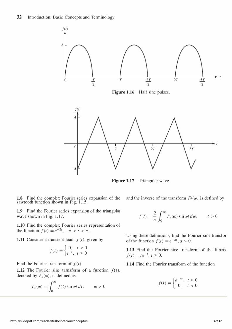
7/17/2019 VibracionConceptos
http://slidepdf.com/reader/full/vibracionconceptos 32/32
32 Introduction: Basic Concepts and Terminology
t
A
0 T T
22T 3T
25T
2
f (t )
Figure 1.16 Half sine pulses.
f (t )
T 2T 3T
A
− A
0t
Figure 1.17 Triangular wave.
1.8 Find the complex Fourier series expansion of thesawtooth function shown in Fig. 1.15.
1.9 Find the Fourier series expansion of the triangular
wave shown in Fig. 1.17.
1.10 Find the complex Fourier series representation of
the function f (t ) = e−2t , −π < t < π .
1.11 Consider a transient load, f (t ), given by
f(t ) =
0, t < 0
e−t , t ≥ 0
Find the Fourier transform of f (t ).
1.12 The Fourier sine transform of a function f(t ),
denoted by F s (ω), is defined as
F s (ω) = ∞
0
f(t ) sin ωt d t, ω > 0
and the inverse of the transform F s (ω) is defined by
f(t ) = 2
π
∞0
F s (ω) sin ωt d ω, t > 0
Using these definitions, find the Fourier sine transform
of the function f (t ) = e−at , a > 0.
1.13 Find the Fourier sine transform of the functio
f(t ) = t e−t , t ≥ 0.
1.14 Find the Fourier transform of the function
f(t ) =
e−at , t ≥ 0
0, t < 0


