University College Dublin An Col aiste ... - maths.ucd.ie
177
University College Dublin An Col´ aiste Ollscoile, Baile ´ Atha Cliath School of Mathematics and Statistics Scoil na Matamaitice agus Staitistic´ ı Applied Mathematics: Mechanics and Methods (ACM 10080) Dr Lennon ´ O N´ araigh Lecture notes in Applied Mathematics: Mechanics and Methods September 2020
Transcript of University College Dublin An Col aiste ... - maths.ucd.ie

University College Dublin
An Colaiste Ollscoile, Baile Atha Cliath
School of Mathematics and StatisticsScoil na Matamaitice agus Staitisticı
Applied Mathematics: Mechanics and Methods(ACM 10080)
Dr Lennon O Naraigh
Lecture notes in Applied Mathematics: Mechanics and Methods September 2020


Applied Mathematics: Mechanics and Methods (ACM10080)
• Subject: Applied and Computational Mathematics
• School: Mathematics and Statistics
• Module coordinator: Dr Lennon O Naraigh
• Credits: 5
• Level: 1
• Semester: First
This module introduces students to the basic principles of Newtonian Mechanics. The module
starts with a description of motion (kinematics) including notions of displacement, velocity, and
acceleration. The module then moves on to an understanding of the causes of motion and changes
in motion (dynamics) via an elementary introduction to Newton’s laws. Key topics here include
force and momentum. Concurrently with this discussion, there will be an introduction to elemen-
tary mathematical methods that can be used to frame all of the above in mathematical language,
including the mathematical treatment of kinematics and dynamics via Calculus, Vectors, and Taylor
series.
What will I learn?
On completion of this module students should be able to
1. Perform mathematical calculations using vectors, including vector addition, scalar multiplica-
tion, and dot products.
2. Use the Cartesian notation for vectors with proficiency.
3. Apply Taylor series as an approximation method in various contexts in Mechanics.
4. Explain comprehensively the notions of vector, velocity, acceleration, momentum, kinetic en-
ergy, potential energy, moment of a force, center of mass, and moments of inertia.
5. Use Newton’s laws to express and solve problems in mathematical terms.
i

ii

Editions
First edition: September 2015
Second edition: September 2019
This edition: September 2020
iii

iv

Acknowledgements
These lecture notes are based almost entirely on previous generations of lecture notes for this module
or for a similar one, written and updated by Professor Joe Pule, Professor Peter Duffy, Professor
Adrian Ottewill, and Professor Peter Lynch.
If I have seen further, it is by standing on the shoulders of giants.
Copyright
All the materials provided in this module are copyright of the Lennon O Naraigh. This means:
• As a user (the student) you have permission (licence) to access the materials to aid and
support your individual studies.
• You are not permitted to edit, adapt, copy or distribute any materials without the relevant
permission.
• As faculty/administration we may reserve the right to remove a user in the event of any
possible infringement.
v

vi

Contents
Abstract i
1 Introduction 1
2 Vectors 3
3 Vectors – representation in Cartesian coordinate systems 14
4 The dot product 23
5 Differential Calculus – Looking back and looking forwards 28
6 Integral Calculus – Looking back and looking forwards 38
7 Kinematics of a particle 48
8 Free-fall motion under gravity 61
9 Forces and Newton’s first two laws of motion 64
10 Newton’s third law of motion 80
11 Statics and Friction 90
12 Mechanical Energy 96
13 Conservation of momentum – application to particle collisions 114
14 Circular motion 120
vii
15 Simple harmonic motion 131
16 A more detailed treatment of extended bodies 156
17 Looking Ahead 166
viii
Chapter 1
Introduction
1.1 Outline
Here is an executive summary of the aims of this module. If you cannot remember the more detailed
outline that follows, at least keep the following in mind:
This module contains two topics:
1. In the first part, we learn or possibly revisit some mathematical methods: vectors and
scalars, differentiation and integration, Taylor series, and Ordinary Differential Equations.
2. In the second part, we apply these methods to frame Newton’s laws of motion for particles
in mathematical language. This enables us to solve problems in mechanics very efficiently.
Or, in more detail, under the heading of mathematical methods:
1. Vectors: We will introduce vectors and scalars. We will formulate these in a mathematical
framework that will enable us to add and subtract vectors, and perform scalar multiplication.
We will introduce the dot product as a way of combining two vectors to get a scalar. We will
introduce a Cartesian framework to perform vector calculations efficiently.
2. Calculus: We will recall some definitions and elementary techniques in Differential and Integral
Calculus. We will apply these techniques below to kinematics and dynamics.
Secondly, under the heading of Mechanics, we will undertake the following work programme:
1. Kinematics: We will describe the concepts of displacement, velocity, and acceleration in
mathematical terms. The study of motion by itself is called kinematics.
1

2 Chapter 1. Introduction
2. Dynamics: We will also study what causes motion and changes in motion. This requires the
introduction of the concepts of force and momentum. This is the study of dynamics, and the
connection between force and momentum is given by Newton’s Laws of motion. Again, this
can all be formulated in mathematical terms.
All of the above will be done for point particles only. Where appropriate, we will demonstrate how
our work can be applied more generally to extended bodies.
3. Work and Energy: We will introduce further concepts that shed more light on the mathematical
underpinning of classical mechanics, including Work and Energy.
4. Applications: We will apply these concepts to various contexts in mechanics, including circular
motion, simple harmonic motion, and the motion of extended bodies.
5. Time permitting, we will also discuss statics, which refers to bodies acted on by forces whose
vector sum is zero. The combined study of statics, kinematics, and dynamics for both particles
and extended bodies can be thought of as Mechanics.
Conceptually, the two headings above split very naturally into two discrete parts. The mathematical
methods section exists on a higher plane of abstraction and is independent of the applications in
mechanics. However, historically, almost all mathematical methods were developed to solve problems
in mechanics. For centuries, it has always felt right to move between one and the other, while
acknowledging the austere beauty of the more abstract mathematical methods. For this reason, we
too will move interchangeably between the two parts of the module. Hopefully this will also reduce
class boredom.
Chapter 2
Vectors
Overview
We define vectors and scalars and give examples. We introduce vector addition using the Parallelo-
gram Law.
2.1 Introduction
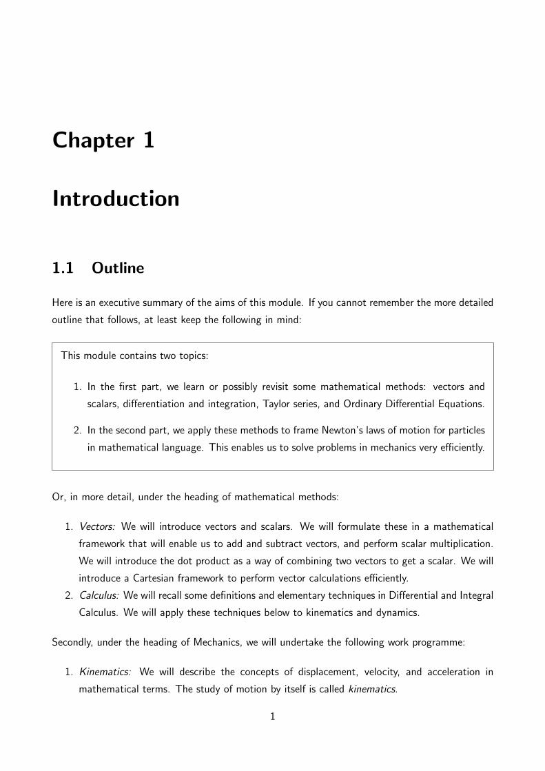
When dealing with motion on a straight line (‘one-dimensional motion’) we will measure things like
distances and speeds with respect to a fixed point of interest, which we call the origin. A particle
can either be to the left or right of the origin. By convention,
• Distances to the right of the origin are positive.
• Distances to the left of the origin are negative.
Displacement is then the signed distance i.e. distance taking direction into account, and Figure 2.1
is just a glorified number line. The question then is how to generalize this to motion in higher
_
O
+
Figure 2.1: Schematic description of one-dimensional displacements with respect to the origin O.
3

4 Chapter 2. Vectors
dimensions (e.g. motion in the plane or in full three-dimensional space). In this context, we need to
be able to measure things like distances and speeds again with respect to a fixed point of interest.
We then need to generalize the number line in Figure 2.1 to planes and full three-dimensional space.
This is where the concept of vectors is needed:
Definition 2.1 Quantities with magnitude and direction are called vectors; quantities with mag-
nitude only are called scalars.
For example, displacement is distance in a particular direction:
5 km ↔ distance ↔ SCALAR
5 km NW ↔ VECTOR
Velocity is speed in a specified direction:
15 km/hr ↔ speed ↔ SCALAR
15 km/hr east ↔ velocity ↔ VECTOR
2.1.1 Quiz
What about the following quantities – vector or scalar?
• Temperature
• Pressure
• Wind
• Energy
• Momentum
2.2 Mathematical description of vectors
A vector can be represented by a directed line segment (Figure 2.2):
• direction of line → gives direction of vector.
• length of line → magnitude of vector.

2.2. Mathematical description of vectors 5
B
A
Arrowhead on lineindicates direction.
Figure 2.2: The vector−→AB represented by a directed line segment. The direction of the vector is
from A to B and the magnitude of the vector corresponds to the length of the line segment from A
to B.
The line segment AB represents a vector denoted by−→AB. The direction of the vector is from A
to B and the magnitude of the vector corresponds to the length of the line segment from A to B.
Thus, vectors−→AB and
−→BA represent two vectors having the same magnigude but opposite directions
(Figure 2.3).
B
A
Arrowhead on lineindicates direction.
(a)
B
A
(b)
Figure 2.3: Vectors−→AB and
−→BA have the same magnitude but opposite directions.
2.2.1 Other notation for vectors:
Vectors are often denoted by boldface type (Figure 2.4).

6 Chapter 2. Vectors
a
In print letters are notunderlined but bold type isused, e.g. a, b, c
Figure 2.4: A vector quantity denoted by a boldface letter ‘a’
There are several other ways to write vectors:
• Arrows:−→AB
• Underbars: a
• Tildes: a
• Others . . .
2.2.2 Relations between vectors
Definition 2.2 Vectors which have the same magnitude and direction are equal.
Definition 2.3 If a has the same magnitude but the opposite direction to b, then a = −b.
a
a = b
bab
a = - b
Figure 2.5: Equality of vectors
Definition 2.4 Let−→AB be a vector. Let the point A be moved through a distance D to produce a
new point A′, and a line segment AA′. Also, let the point B be moved through the same distance
D and in parallel to the line segment AA′ to produce a new point B′. Then the vector−−→A′B′ is the
vector−→AB parallel-transported through distance D – see Figure 2.6.

2.2. Mathematical description of vectors 7
Figure 2.6: Parallel transport of the vector−→AB.
By definition 2.2 the vector−→AB and its parallel-transported version
−−→A′B′ are equal. Parallel-transport
of a vector leaves the vector unchanged. This is very much like the idea in geometry of congruent
triangles. In particular, two triangles that can be parallel-transported so that they coincide are
congruent. Thus, equality of vectors can be thought of as being like congruency – it is a coincidence
of two geometric objects that is brought about by a geometric transformation.
Definition 2.5 Let λ be a real number and let−→AB be a vector. Then λ(
−→AB) is also a vector, with
the following properties:
• The magnitude of the new vector is |λ||AB|.
• Direction:
– If λ > 0, then the direction of the new vector is the same is the direction of the old one,
i.e. from A to B.
– If λ < 0, then the direction of the new vector is the opposite as that of the old one, i.e.
from B to A.
Then λ(−→AB) is called a scalar multiple of
−→AB.

8 Chapter 2. Vectors
Geometrically, λ−→AB can be parallel-transported so that it is collinear with
−→AB and points either in
the same direction as−→AB or in the opposite direction. Thus, scalar multiplication of a vector results
in a new vector, parallel or anti-parallel to the starting vector. For examples, see Figure 2.7
a
b = a
c = a
2
_12
c
b
Figure 2.7: Scalar multiples of the vector a
2.3 Addition of vectors – parallelogram law
In what follows, it will be very helpful to be able to add two vectors together. There is a recipe for
doing this called the parallelogram law of vector addition, which starts with two vectors a =−→AB
and b =−−→XY and generates the vector sum a + b:
1. Parallel-transport the two vectors so that their bases coincide, and such that
a =−→OA, b =
−−→OB.
See Figure 2.8(a).
2. Form a parallelogram OACB by further parallel-transport operations (Figure 2.8(b)):
• Parallel-transport the vector a through the vector b to produce a new vector−−→BC;
• Parallel-transport the vector b through the vector a to produce a new vector−→AC.

2.3. Addition of vectors – parallelogram law 9
3. The vector−→OC is the sum a + b (Figure 2.8).
(a) (b) (c)
Figure 2.8: Parallelogram law of vector addition
A nice feature of this law is that the vectors a and b are used interchangeably – neither a nor b
are singled out for special treatment in the definition. Therefore, it follows that a + b = b + a,
and a familiar property of (ordinary) addition is retained here, namely that the vector addition is
commutative.
Furthermore, because the vectors b and b′ :=−→AC are the same vector (by parallel transport), we
can formulate a totally equivalent (but sometimes more convenient) recipe for adding vectors called
the triangle law of vector addition, which can be summarized in the following sequence of steps:
1. Parallel-transport the two vectors so that the base of b coincides with the tip of a, such that,
under parallel transport,
a =−→OA, b = b′ =
−→AC.
2. Consider the resulting triangle OAC. The vector−→OC is the vector sum a + b.
The triangle law gives a good way of thinking addition of two arbitrary vectors is in terms of the
particular vector displacement. Suppose I walk from O to A and from A to C. The net effect of my
journey is the same as if I would travel directly from O to C. This is my displacement. So my net
displacement can be got from vector addition of the two vectors−→OA and
−→AC. Mathematically,
−→OA+
−→AC =
−→OC.

10 Chapter 2. Vectors
DO
BA
Ca
b c
d
e
Figure 2.9: Any number of vectors can be added by successive application of the parallelogram law.
Any number of vectors can be added by successive application of the parallelogram law. For example,
in Figure 2.9 we have
e = a + b + c + d
or−−→OD =
−→OA+
−→AB +
−−→BC +
−−→CD
The order in which these applications are done does not matter, i.e.
e = (a + b) + (c + d),
= [(a + b) + c] + d, etc.
This is another familiar property of addition that is reproduced by the vector addition operation.
At this point, it is helpful to introduce the notion of the zero vector: this is a vector with zero
magnitude and arbitrary direction, and is denoted simply by 0, as with ordinary real numbers.
Consider for a moment the vector sum a+ b. One can imagine shrinking down the magnitude of b
until it becomes the zero vector. From the triangle law, one can see that as b is shrunk to the zero
vector, the sum a + b reduces simply to a. Hence,
a + 0 = a.
Finally, vectors can also be subtracted: a − b means the same thing as the vector addition of
a + (−b), where −b is the vector b with its direction reversed. From the triangle law, it follows
that a− a = 0.
Interestingly, we may summarize the properties of the vector addition, valid for all vectors a, b, and
c:
1. Closure: The sum of any two vectors is also a vector: by the parallelogram law in Figure 2.8,
the sum a + b is a quantity with both magnigude and direction, and is therefore yet another
vector.

2.4. Worked examples 11
2. Associative:
(a + b) + c = a + (b + c) = a + b + c,
3. Existence of zero vector 0, such that
a + 0 = a
4. Existence of inverses: for each vector a, we have
a + (−a) = 0.
5. Commutative:
a + b = b + a.
Later on you will see that these properties make the set of all vectors into a mathematical structure
called an Abelian group.
2.4 Worked examples
M
a
b
C
B
A
Example: Refer to the figure. The point
M is at the mid-point of AC Find, in
terms of a and b
−→AC,
−→CA,
−−→AM,
−−→MB.

12 Chapter 2. Vectors
Solution:
−→AB = a
−−→BC = b
(a)−→AC =
−→AB +
−−→BC = a + b
(b)−→CA = −
−→AC = −(a + b)
(c)−−→AM =
1
2
−→AC =
1
2(a + b)
(d)−−→MB =
−−→MA+
−→AB
= −−−→AM +
−→AB
= −1
2(a + b) + a
= −1
2a− 1
2b + a
=1
2a− 1
2b =
1
2(a− b) .
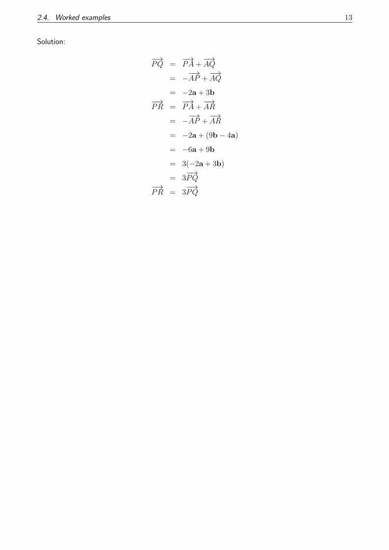
P
2a
3b
A
Q
R9b - 4a
Example: Refer to the figure. A, P , Q
and R are four points:
−→AP = 2a−→AQ = 3b−→AR = 9b− 4a
Show that P , Q and R are co-linear.
2.4. Worked examples 13
Solution:
−→PQ =
−→PA+
−→AQ
= −−→AP +
−→AQ
= −2a + 3b−→PR =
−→PA+
−→AR
= −−→AP +
−→AR
= −2a + (9b− 4a)
= −6a + 9b
= 3(−2a + 3b)
= 3−→PQ
−→PR = 3
−→PQ

Chapter 3
Vectors – representation in Cartesian
coordinate systems
Overview
In the last section we introduced vectors and vector addition. The discussion was a little bit on
the qualitative side. A convenient way to make this discussion more formal and to enable efficient
computations is to represent vectors in a Cartesian coordinate system. This is the subject of this
chapter.
3.1 Components of a vector
O
C
B
A
c
b
a
It is useful to split up a vector into its com-
ponents. This is called resolving the vector
into components. To see what these terms
mean, consider the figure on the left, where
we have c = a + b. Then
c is the resultant of the vectors a and b.
a and b are the components of c.
Usually we resolve a vector in two orthogonal (perpendicular) components – as in Figure 3.1.
14

3.1. Components of a vector 15
B
AO
C
p
q
If
• the magnitude of−−→OB is p (we write |
−−→OB| = p) and
• the magnitude of−→OA is q (we write |
−→OA| = q)
then
|−→OC| =
√p2 + q2. (3.1)
We will discuss Equation (3.1) in more detail below. However, we first of all introduce distinguished
vectors to help us resolve any vector into orthogonal components. To do this, we need the notion
of a unit vector:
Definition 3.1 A vector of magnitude one is called a unit vector.
More specifically, we have the following two distinguished unit vectors in a specific Cartesian coor-
dinate system:
Definition 3.2 In the x-y plane, unit vectors in the Ox and Oy directions are denoted by i and j.
Any vector in the x-y-plane can be resolved in terms of i and j – e.g. Figure 3.1.

16 Chapter 3. Vectors – representation in Cartesian coordinate systems
y
xO
B
A
(a)−−→AB = 2i+ 5j
y
xO
P
Q
(b)−−→PQ = 2i− 5j
In general, a vector a is represented in terms of the unit vectors i and j as
a = a1i + a2j,
where a1 and a2 are real numbers. Addition and subtraction of vectors then become very easy –
and the machinery of the parallelogram law can be placed firmly in the background. For example,
Theorem 3.1 Let a = a1i+a2j and b = b1i+ b2j be two co-planar vectors, and let a+b be given
by the paralllelogram law of vector addition. Then
a + b = (a1 + b1)i + (a2 + b2)k.
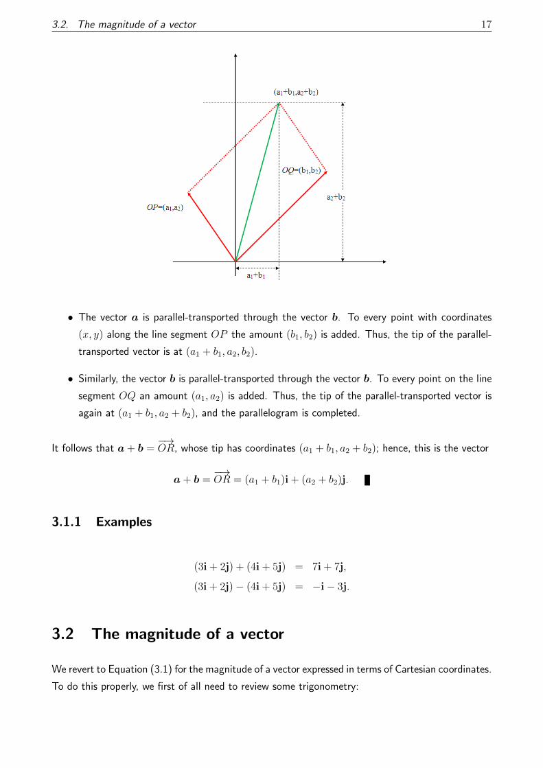
Proof: Refer to Figure 3.1. The vectors a and b are already positioned such that their bases coincide.
A parallelogram is completed by parallel transport:
3.2. The magnitude of a vector 17
• The vector a is parallel-transported through the vector b. To every point with coordinates
(x, y) along the line segment OP the amount (b1, b2) is added. Thus, the tip of the parallel-
transported vector is at (a1 + b1, a2, b2).
• Similarly, the vector b is parallel-transported through the vector b. To every point on the line
segment OQ an amount (a1, a2) is added. Thus, the tip of the parallel-transported vector is
again at (a1 + b1, a2 + b2), and the parallelogram is completed.
It follows that a + b =−→OR, whose tip has coordinates (a1 + b1, a2 + b2); hence, this is the vector
a + b =−→OR = (a1 + b1)i + (a2 + b2)j.
3.1.1 Examples
(3i + 2j) + (4i + 5j) = 7i + 7j,
(3i + 2j)− (4i + 5j) = −i− 3j.
3.2 The magnitude of a vector
We revert to Equation (3.1) for the magnitude of a vector expressed in terms of Cartesian coordinates.
To do this properly, we first of all need to review some trigonometry:

18 Chapter 3. Vectors – representation in Cartesian coordinate systems
θ
Hypoten
use
Adjacent
Opposite
sin(θ) =O
H
cos(θ) =A
H
tan(θ) =O
A
How do you remember this?
Silly Old Harry Caught A Herring Trawling Off America
Two Old Angels Sitting On High Chatting About Heaven
sock a toe-a (SOHCAHTOA)
Tom’s Old Aunt Sat On Her Coat And Hat
sin, cos, tan: Orace Had A Heap Of Apples
I went to a Gaelscoil, so we had
sin(θ) =urcoireach
taobhagan, cos(θ) =
congrach
taobhagan, tan(θ) =
urcoireach
congrach,
and
sin, cos, tan: Under The Crappy Teacher’s Useless Car
which was certainly no comment on my mathematics teacher, who was outstanding. In any event,
for an arbitrary vector a =−→OA expressed in Cartesian coordinates as
a = a1i + a2j,
the magnitude of the vector is the length of the line segment OA, which by Pythagoras’s theorem
is
|OA| =√a2
1 + a22,
hence
magnitude of a ≡ |a| ≡ |−→OA| =
√a2
1 + a22,
which is simply Equation (3.1) re-expressed in slightly different notation. An example of a magnitude
calculation is shown in Figure 3.1.

3.2. The magnitude of a vector 19
y
xO
P
Q
Figure 3.1: |−→PQ| = |2i− 5j| =
√4 + 25 =
√29
3.2.1 Worked examples
A plane taking off at an angle of 30◦ to
the runway at 36 km/hr. Find the veloc-
ity components.
Solution: The vectors in the figure and their associated magnitudes are converted into an abstract
trigonometric problem in Figure 3.2 below.

20 Chapter 3. Vectors – representation in Cartesian coordinate systems
1
2
30
Figure 3.2:
We have,
36 km/hr = 36×100060×60
= 360003600
= 10 m/s.
Horizontal component: PQ = 10 cos 30◦ = 10√
32
= 8.7 m/s.
Vertical component: QR = 10 sin 30◦ = 10√
12
= 5 m/s.
Example: v is in the direction of the vector 12i− 5j and has magnitude 39. Find v.
Solution: v must be a multiple of 12i− 5j, so we have
v = k(12i− 5j) k > 0
= 12ki− 5kj
|v|2 = 144k2 + 25k2
= 169k2
|v| = 13k = 39 k = 3
v = 36i− 15j
Example: Let p = 4i − 3j and q = −12i + 5j. The vector v has the same direction as p − q
and has half the size of p + q. Find v.
Solution: We have
p− q = (4 + 12)i + (−3− 5)j = 16i− 8j.
Also,
p + q = (4− 12)i + (−3 + 5)j = −8i + 2j,
3.2. The magnitude of a vector 21
with
|p + q| =√
82 + 22 =√
68.
In the question, we are given that
v = k(p− q) = k(16i− 8j), k > 0,
hence
|v| = k√
162 + 642 = k√
320.
But |v| = (1/2)|p + q| from the question, hence
|v| = (1/2)√
68 = k√
320,
and
k = 12
√68
320=
√68
4× 320=
√17
320.
Thus
v = k(16i− 8j) =
√17
320(16i− 8j),
which is the final answer.
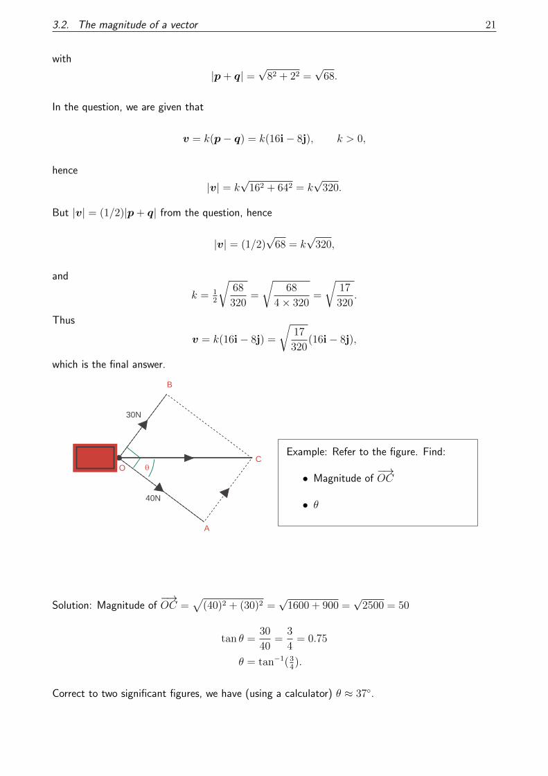
B
A
30N
40N
OC
Example: Refer to the figure. Find:
• Magnitude of−→OC
• θ
Solution: Magnitude of−→OC =
√(40)2 + (30)2 =
√1600 + 900 =
√2500 = 50
tan θ =30
40=
3
4= 0.75
θ = tan−1(34).
Correct to two significant figures, we have (using a calculator) θ ≈ 37◦.

22 Chapter 3. Vectors – representation in Cartesian coordinate systems
B
A
O
C
N
12
12
7
7
Example: Refer to the figure. Find the
resultant (magnitude and α) of two ve-
locities 7 km/hr SW and 12 km/hr SE.
Solution: We have
|−→OC|2 = (12)2 + 72
= 144 + 49 = 193
|−→OC| =
√193
Correct to three significant figures this is 13.9: Resultant has magnitude 13.9 km/hr (correct to
three significant figures). Also,
tan θ = 7/12
θ = tan−1( 712
)
α = π2
+ π4
+ θ = 3π4
+ θ.
Thus,
α = 3π4
+ tan−1( 712
).
Correct to three significant figures, this is
α = 165.3◦, correct to three significant figures.
Chapter 4
The dot product
Overview
We introduce a kind of multiplication between two vectors that takes in two vectors and returns
a scalar quantity. This is called the dot product. The dot product provides a very useful way of
computing the magnitude of a vector.
4.1 The definition
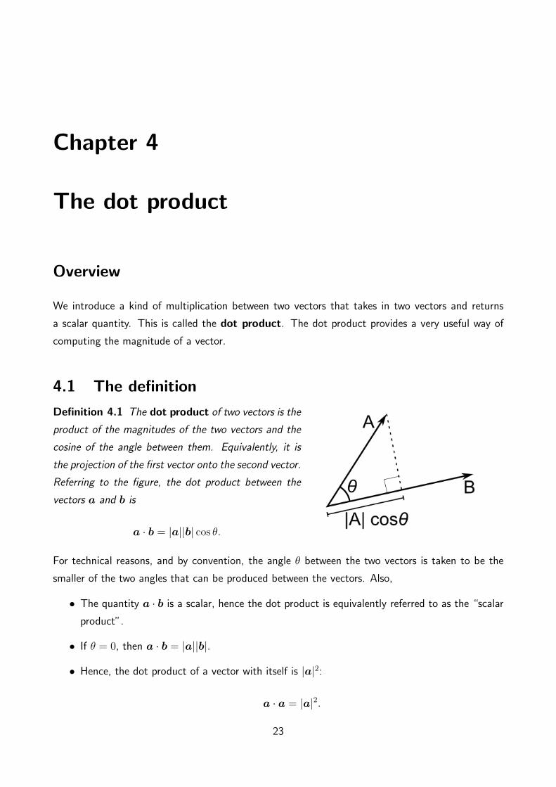
Definition 4.1 The dot product of two vectors is the
product of the magnitudes of the two vectors and the
cosine of the angle between them. Equivalently, it is
the projection of the first vector onto the second vector.
Referring to the figure, the dot product between the
vectors a and b is
a · b = |a||b| cos θ.
For technical reasons, and by convention, the angle θ between the two vectors is taken to be the
smaller of the two angles that can be produced between the vectors. Also,
• The quantity a · b is a scalar, hence the dot product is equivalently referred to as the “scalar
product”.
• If θ = 0, then a · b = |a||b|.
• Hence, the dot product of a vector with itself is |a|2:
a · a = |a|2.
23

24 Chapter 4. The dot product
Thus, another way to look at the magnitude of a vector is as follows:
magnitude of a ≡ |a| =√a · a.
• Just as importantly, if θ = π/2, then a · b = 0: two vectors are are right angles (orthogonal)
if and only if a · b = 0.
The dot product is also very intimately connected to the cosine rule, as the following theorem shows:
Theorem 4.1 Let c = b− a. Then
a · b = 12
(|a|2 + |b|2 − |c|2
).
Proof: Refer to the figure, noting in particular the vec-
tor c = b− a. By the cosine rule,
|c|2 = |a|2 + |b|2 − 2|a||b| cos θ
= |a|2 + |b|2 − 2a · b.
Re-arranging gives
a · b = 12
(|a|2 + |b|2 − |c|2
).
c
b
a
4.2 The dot product in a Cartesian coordinate system
Now, the neatest thing of all about the dot product is that it is very easily computed in Cartesian
coordinates:
Theorem 4.2 Let a = a1i + a2j and let b = b1i + b2j be two co-planar vectors. Then
a · b = a1b1 + a2b2.
Proof: Refer to Figure 4.1.
We have
c = b− a = (b1 − a1)i + (b2 − a2)j.

4.3. Worked examples 25
Figure 4.1: Sketch for the proof of Theorem 4.2
Using Theorem 4.1 we have
a · b = 12
(|a|2 + |b|2 − |c|2
),
= 12
{(a2
1 + a22
)+ (b2
1 + b22)−
[(b1 − a1)2 + (b2 − a2)2
]},
= 12
[a2
1 + a22 + b2
1 + b22 − b2
1 − a21 + 2a1b1 − b2
2 − a22 + 2b2a2
].
Tidying up, this is
a · b = a1b1 + a2b2.
4.3 Worked examples
Example: If a = 2i + 3j and b = 4i + 15j, find a · b.
Solution:
a · b = (2i + 3j) · (4i + 15j),
= 2× 4 + 3× 15,
= 53.

26 Chapter 4. The dot product
Example: Let a = 3i + j and b = i− j. Find the angle between a and b.
Solution: we have |a| =√
32 + 1 =√
10 and |b| =√
2. Also, a · b = 3− 1 = 2. We now use
a · b = |a||b| cos θ =⇒ cos θ =a · b|a||b|
to write
cos θ = 2√10√
2=√
420
= 1√5,
hence
θ = cos−1(
15
).
Example: Find a unit vector perpendicular to a = i + 3j.
Solution: let b = xi + yj be the required vector. We have a · b = 0, hence
x+ 3y = 0,
hence x = −3y. Thus, the vector can be rewritetn as b = y(−3i+ j). The second condition is that
this is a unit vector, such that b · b = 1, or
y2(3 · 3 + 1 · 1) = 1,
hence y2 = 1/10, hence y = ±1/√
10, and the positive sign is chosen (this is an arbitary choice).
Thus, the required vector is
b = 1√10
(−3i + j) .
4.3. Worked examples 27
A
B CE
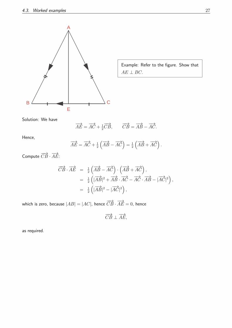
Example: Refer to the figure. Show that
AE ⊥ BC.
Solution: We have−→AE =
−→AC + 1
2
−−→CB,
−−→CB =
−→AB −
−→AC.
Hence,−→AE =
−→AC + 1
2
(−→AB −
−→AC)
= 12
(−→AB +
−→AC).
Compute−−→CB ·
−→AE:
−−→CB ·
−→AE = 1
2
(−→AB −
−→AC)·(−→AB +
−→AC),
= 12
(|−→AB|2 +
−→AB ·
−→AC −
−→AC ·
−→AB − |
−→AC|2
),
= 12
(|−→AB|2 − |
−→AC|2
),
which is zero, because |AB| = |AC|, hence−−→CB ·
−→AE = 0, hence
−−→CB ⊥
−→AE,
as required.

Chapter 5
Differential Calculus – Looking back and
looking forwards
Overview
Differential Calculus is the mathematical study of change, in the same way that geometry is the
study of shape and algebra is the study of operations and their application to solving equations.
The reason for including the review here and in the next chapter is to put all students on a level
playing field: some students may have already seen this material in either the Leaving Certificate or
MATH10350 – or both, or neither, so the review here will help all students to have access to the
same theoretical tools for doing mechanics. That being said, the review here will be fast-paced.
5.1 Introduction – via the slope of a graph
We start of by studying the slope of a straight line y = mx+ c. We want to know how y changes
as x changes:
Referring to the figure on the right, the slope or
gradient is the “rise over run”:
m =y2 − y1
x2 − x1
=∆y
∆x
28
5.1. Introduction – via the slope of a graph 29
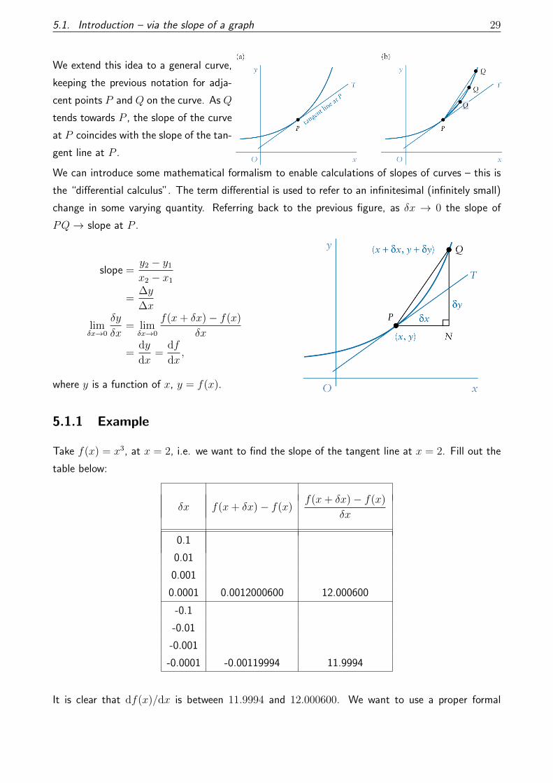
We extend this idea to a general curve,
keeping the previous notation for adja-
cent points P and Q on the curve. As Q
tends towards P , the slope of the curve
at P coincides with the slope of the tan-
gent line at P .
We can introduce some mathematical formalism to enable calculations of slopes of curves – this is
the “differential calculus”. The term differential is used to refer to an infinitesimal (infinitely small)
change in some varying quantity. Referring back to the previous figure, as δx → 0 the slope of
PQ→ slope at P .
slope =y2 − y1
x2 − x1
=∆y
∆x
limδx→0
δy
δx= lim
δx→0
f(x+ δx)− f(x)
δx
=dy
dx=
df
dx,
where y is a function of x, y = f(x).
5.1.1 Example
Take f(x) = x3, at x = 2, i.e. we want to find the slope of the tangent line at x = 2. Fill out the
table below:
δx f(x+ δx)− f(x)f(x+ δx)− f(x)
δx
0.1
0.01
0.001
0.0001 0.0012000600 12.000600
-0.1
-0.01
-0.001
-0.0001 -0.00119994 11.9994
It is clear that df(x)/dx is between 11.9994 and 12.000600. We want to use a proper formal

30 Chapter 5. Differential Calculus – Looking back and looking forwards
calculation to show this:
f(x) = x3
df(x)
dx= lim
δx→0
[f(x+ δx)− f(x)
δx
]= lim
δx→0
(x+ δx)3 − x3
δx
= limδx→0
x3 + 3x2δx+ 3xδx2 + δx3 − x3
δx
= limδx→0
(3x2 + 3xδx+ δx2)
= 3x2
So, for x = 2, we have df(x)dx
= 3(2)2 = 12.
5.1.2 Extension to xn, n ∈ N
Take f(x) = xn:
df(x)
dx= lim
δx→0
(x+ δx)n − xn
δx
Binomial theorem:
(x+ y)n = xn +
(n
1
)xn−1y1 +
(n
2
)xn−2y2 + · · ·+
(n
n− 1
)x1yn−1 + yn,
(nk
)= ”n choose k” = n!
k!(n−k)!
df(x)
dx= lim
δx→0
xn +(n1
)xn−1δx1 + · · ·+ δxn − xn
δx= nxn−1
So, when we differentiate xn we get:df
dx= nxn−1 (5.1)
Later on we shall show that Equation (5.1) holds for all real n; with n < 1 the equation holds for
all x 6= 0. In particular, for x 6= 0 and n = −1, we have
d
dx(x−1) = −x−2 = − 1
x2. (5.2)

5.2. Important properties of the derivative 31
5.1.3 Derivative of a constant function
Suppose that f(x) = k, where k is a real constant. What is df/dx? Well, note that
f(x) = k,
f(x+ δx) = k,
hence
f(x+ δx)− f(x) = k − k = 0,
hence
limδx→0
[f(x+ δx)− f(x)
δx
]= lim
δx→0
[0
δx
]= 0
and so we have proved the following important theorem:
Theorem 5.1 The derivative of a constant function is zero at all points.
In particular, since f(x) = x0 = 1 is a constant function, the derivative of f(x) = x0 is zero, for all
x ∈ R.
5.2 Important properties of the derivative
Theorem 5.2 (Linearity) Let u(x) and v(x) be functions and a and b be constants. Then,
d(au(x) + bv(x))
dx= a
du(x)
dx+ b
dv(x)
dx.
Proof:
d(au(x) + bv(x))
dx= lim
δx→0
au(x+ δx) + bv(x+ δx)− au(x)− bv(x)
δx
=a limδx→0
u(x+ δx)− u(x)
δx+ b lim
δx→0
v(x+ δx)− v(x)
δx
=adu(x)
dx+ b
dv(x)
dx.
In this way, we can extend the rule (d/dx)xn = nxn−1 for n ∈ N to any polynomial. In particular,
for a straight line u(x) = mx+ c, this can be thought of as u(x) = mx1 + cx0, hence
df
dx= m
(d
dxx1
)+ c
(d
dxx0
)= m = slope of line.

32 Chapter 5. Differential Calculus – Looking back and looking forwards
Theorem 5.3 (Product rule) Let u(x) and v(x) be two functions of x. Then
d(u(x)v(x))
dx= u(x)
dv(x)
dx+
du(x)
dxv(x).
Proof: We have
d(u(x)v(x))
dx= lim
δx→0
u(x+ δx)v(x+ δx)− u(x)v(x)
δx
= limδx→0
u(x+ δx)v(x+ δx) + u(x+ δx)v(x)− f(x+ δx)v(x)− u(x)v(x)
δx
= limδx→0
u(x+ δx)v(x+ δx)− u(x+ δx)v(x)
δx
limδx→0
u(x+ δx)v(x)− u(x)v(x)
δx
=(
limδx→0
u(x+ δx))(
limδx→0
v(x+ δx)− v(x)
δx
)(
limδx→0
u(x+ δx)− u(x)
δx
)v(x)
= u(x)dv(x)
dx+
du(x)
dxv(x).
Theorem 5.4 (Quotient rule) Let u(x) and v(x) be two functions of x, such that v(x) 6= 0 on
the domain of interest. Thend
dx
(uv
)=v du
dx− udv
dx
v2.
Proof: We have
d
dx
(uv
)= lim
δx→0
1
δx
[u(x+ δx)
v(x+ δx)− u(x)
v(x)
],
= limδx→0
1
δx
[u(x+ δx)
v(x+ δx)+u(x+ δx)
v(x)− u(x+ δx)
v(x)− u(x)
v(x)
],
= limδx→0
1
δx
{u(x+ δx)
[1
v(x+ δx)− 1
v(x)
]+
1
v(x)[u(x+ δx)− u(x)]
}= lim
δx→0
1
δx
{− u(x+ δx)
v(x+ δx)v(x)[v(x+ δx)− v(x)] +
1
v(x)[u(x+ δx)− u(x)]
},
= limδx→0
{− u(x+ δx)
v(x+ δx)v(x)
[v(x+ δx)− v(x)
δx
]+
1
v(x)
[u(x+ δx)− u(x)
δx
]}.
We now use the algebra of limits to rewrite this as
d
dx
(uv
)= −
[limδx→0
u(x+ δx)
v(x+ δx)v(x)
] [limδx→0
v(x+ δx)− v(x)
δx
]+
1
v(x)
[limδx→0
u(x+ δx)− u(x)
δx
],
henced
dx
(uv
)= − 1
v2
dv
dx+
1
v
du
dx
5.2. Important properties of the derivative 33
Tidying up, this isd
dx
(uv
)=v du
dx− udv
dx
v2.
Example: Let u(x) = 3x2 + 2x + 1 and let v(x) = 4x + 2. Verify the product rule in this
instance by computing (d/dx)u(x)v(x) in two independent ways.
Solution: we have
u(x)v(x) = (3x2 + 2x+ 1)(4x+ 2),
= 12x3 + 6x2 + 8x2 + 4x+ 4x+ 2,
= 12x3 + 14x2 + 8x+ 2.
Hence, by linearity of the derivative,
d
dxuv = 36x2 + 28x+ 8.
Independently, using the product rule, we have
d
dxuv = u
dv
dx+ v
du
dx,
= (3x2 + 2x+ 1)× 4 + (4x+ 2)× (6x+ 2),
= 12x2 + 8x+ 4 + 24x2 + 20x+ 4,
= 36x2 + 28x+ 8,
and the two methods (obviously) agree.
Example: Let u(x) = x3 + 3x and let v(x) = x2 + 1, with v(x) never zero. Compute the value
of (d/dx)(u/v) at x = 0.
Solution: Using the quotient rule, we have
d
dx
(uv
)=v du
dx− udv
dx
v2,
=(x2 + 1)(3x2 + 3)− (x3 + 3x)2x
(x2 + 1)2,
=3(x2 + 1)2 − 2x(x3 + 3x)
(x2 + 1)2,
= 3− 2x2(x2 + 3)
(x2 + 1)2.

34 Chapter 5. Differential Calculus – Looking back and looking forwards
At x = 0 this is simply [d
dx
(uv
)]x=0
= 3.
5.3 The chain rule
A vital ability in Differential Calculus is to be able to differentiate a ‘function of a function’. Specif-
ically, let u(x) and v(x) be functions. We are interested in the composition
y(x) = u(v(x)),
and the derivative dy/dx. Before learning a potentially dangerous shortcut to the answer, it is
helpful to express the answer in a more correct way, by way of the following new notation for the
derivative:
Definition 5.1 (Alternative notation for the derivative) Let u(x) be a function. Then the
derivative du/dx is also written equivalently as u′(x):
u′(x) = limδx→0
u(x+ δx)− u(x)
δx.
Now we have the following theorem:
Theorem 5.5 (Chain rule) Let u(x) and v(x) be functions. Form the composition y(x) =
u(v(x)). Then
y′(x) = u′(v(x))v′(x).
Proof:
dy
dx= lim
δx→0
u(v(x+ δx))− u(v(x))
δx,
= limδx→0
[u(v(x+ δx)− u(v(x))
v(x+ δx)− v(x)
]×[v(x+ δx)− v(x)
δx
].
We write δv = v(x+ δx)− v(x) and note that δv → 0 as δx→ 0. Hence, the above limit can be
re-written as
dy
dx=
[limδv→0
u(v(x+ δx)− u(v(x))
v(x+ δx)− v(x)
]×[
limδx→0
v(x+ δx)− v(x)
δx
],
= u′(v(x))v′(x).

5.3. The chain rule 35
Now, for the potentially harmful shorthand: reverting back to the old “dee-by-dee-x” notation for
the derivative, the chain rule can be expressed as
dy
dx=
du
dv
dv
dx.
This formula is often conceptualized as an equality where the “dv cancels above and below”. This
is a very useful intellectual shortcut to the correct answer but it is also technically wrong, so care is
needed here.
Example: Let u(x) = 3x2 + 2x+ 1 and let v(x) = 4x+ 2. Verify the chain rule in this instance
by computing (d/dx)u(v(x)) in two independent ways.
We compute y(x) = u(v), where v = 4x+ 2. We have:
y(x) = u(v),
= 3v2 + 2v + 1,
= 3(4x+ 2)2 + 2(4x+ 2) + 1,
= 3(16x2 + 16x+ 4) + 8x+ 4 + 1,
= 48x2 + 56x+ 17,
hencedy
dx= 96x+ 56.
Separately,
dy
dx=
du
dv
dv
dx,
=
[d
dv
(3u2 + 2u+ 1
)]× 4,
= 4 (6v + 2) ,
= 24v + 8,
= 24(4x+ 2) + 8,
= 96x+ 56,
and the two methods (rightly) agree.

36 Chapter 5. Differential Calculus – Looking back and looking forwards
Example: Let v(x) 6= 0 be a function. Show in two separate ways that
d
dx
(1
v(x)
)= − 1
v2
dv
dx.
Solution: Using the quotient rule with u(x) = 1 and hence du/dx = 0, we have
y(x) =u(x)
v(x)=
1
v(x),
and
dy
dx=
v × 0− 1× dvdx
v(x)2,
= − 1
v2
dv
dx.
Separately, let u(x) = 1/x and let
y(x) = u(v(x)) =1
v(x).
Then,
dy
dx=
d
dx
(1
v(x)
),
=d
dv
dv
dx,
=
(d
dv
1
v
)dv
dx,
=
(d
dvv−1
)dv
dx,
=(−v−2
) dv
dx,
, = − 1
v2
dv
dx.

5.3. The chain rule 37
Example: Let y(x) = 1/x2. Compute du/dx for x 6= 0.
Solution: From before, let v(x) = x2, hence y(x) = 1/v(x). We have
dy
dx=
d
dx
1
v(x),
= − 1
v2
dv
dx,
= − 1
x4× (2x),
= − 2
x3.
Example: Let y(x) =√
5x− 8, with 5x− 8 > 0. Compute y′(x).
Solution: Write y(x) = (5x − 8)1/2 and further write y(x) = u(v(x)). Identify u(v) = v1/2, and
v(x) = 5x− 8. We have
dy
dx=
du
dv
dv
dx,
=
(d
dvv1/2
)[d
dx(5x− 8)
],
=(
12v−1/2
)× 5,
= 52(5x− 8)−1/2,
hence
y′(x) = 52
1√5x− 8
.

Chapter 6
Integral Calculus – Looking back and
looking forwards
Overview
We review integral calculus, paying particular attention to the Fundamental Theorem of Calculus
and integration by substitution.
6.1 Definition as the anti-derivative
One way to introduce the Integral Calculus is through the anti-derivative:
Let F (x) = df/dx be a known function. Find f(x).
In this context, f(x) is called the anti-derivative of F (x):
F (x) =df
dx=⇒ f(x) =
∫F (x) dx.
The notation∫F (x) dx means ‘the function whose derivative is F (x)’. By definition, have
f(x) =
∫F (x) dx,
=
∫df
dxdx (6.1)
38

6.1. Definition as the anti-derivative 39
Also,
F (x) =df
dx,
=d
dx
∫F (x) dx. (6.2)
The process of finding the anti-derivative is called integration. Equations (6.1)–(6.2) are the math-
ematical statement that integration and differentiation are inverses of each other: if you compose
these two operations on a function f(x), you end up where you started, i.e. with f(x) again.
6.1.1 The constant of integration
Let F (x) = df/dx and let
f(x) =
∫F (x) dx
be an anti-derivative. Consider also a second candidate for the anti-derivative.
h(x) =
∫F (x) dx+ C,
where C is a constant. Then,df
dx= F (x),
dh
dx= F (x),
and both f(x) and h(x) are equally good anti-derivatives for F (x). Thus, the anti-derivative is
only defined up to a constant C, which we call the constant of integration. We write the general
anti-derivative as
f(x) =
∫F (x) dx+ C
to indicate this slight imprecision in the definition.
6.1.2 Elementary anti-derivatives
Because of the definition of integration as the anti-derivative, we can work out some expressions for
anti-derivatives of elementary functions:
• Elementary powers:∫xn dx =
1
n+ 1xn+1 + C ⇐⇒ d
dx
(1
n+ 1xn+1
)= xn, n 6= −1.
• Exponential: ∫ex dx = ex + C ⇐⇒ d
dxex = ex.

40 Chapter 6. Integral Calculus – Looking back and looking forwards
• x−1: ∫1
xdx = log x+ C ⇐⇒ d
dxlog x =
1
x.
• sin(x): ∫sinx dx = − cosx+ C ⇐⇒ d
dx(− cosx) = sinx.
Note the sign!
• cos(x): ∫cosx dx = sinx+ C ⇐⇒ d
dx(sinx) = cos x.
• Linearity: Because differentiation is linear, the integral is as well.
a
∫F (x) dx+ b
∫G(x) dx =
∫(aF (x) + bg(x)) dx. (6.3)
Theorem 6.1 (Linearity) Integration is a linear operation, i.e. Equation (6.3) holds.
Proof: Let
f(x) =
∫F (x) dx+ C, g(x) =
∫G(x) dx+D
Then for a and b constant,
af(x) + bg(x) = a
∫F (x) dx+ b
∫G(x) dx+ Const.
Differentiate both sides of this expression to obtain
d
dx[af(x) + bg(x)] = a
d
dx
∫F (x) dx+ b
d
dx
∫G(x) dx,
where we have (crucially) used the linearity property of the derivative here. By definition of the
anti-derivative, this isd
dx[af(x) + bg(x)] = aF (x) + bG(x).
Again, by definition of the anti-derivative,
af(x) + bg(x) =
∫[aF (x) + bG(x)] dx.
But this is
a
∫F (x) dx+ b
∫G(x) dx =
∫[aF (x) + bG(x)] dx,
up to a constant, so Equation (6.3) is shown.

6.2. Worked examples 41
6.2 Worked examples
Example: Find the anti-derivative of 2x2.
Solution: The anti-derivative is ∫2x2, dx.
By linearity, the constant comes outside the integral:∫2x2 dx = 2
∫x2 dx = 2
3x3 + Const.
Example: Find the anti-derivative of x2 + 2 cosx.
Solution: The anti-derivative is ∫(x2 + 2 cosx) dx.
By linearity, this splits up:∫(x2 + 2 cosx) dx =
∫x2 dx+ 2
∫cos(x) dx = 1
3x3 + 2 sinx.
6.3 The definite integral and area
Definition 6.1 (Definite integral) Let F (x) = df/dx and let f(x) =∫F (x) dx + C be an
anti-derivative. The quantity f(b) − f(a) is called the definite integral of F (x) between a and b;
we write
f(b)− f(a) =
∫ b
a
F (x) dx. (6.4)
There is a lot of notation to take in in Equation (6.4)
• a and b are called the limits of integration.
• a is called the lower limit; b is called the upper limit.
• F (x) is called the integrand.
One of the most stunning results of all of Mathematics goes by the name of the Fundamental
Theorem of Calculus. You will be introduced to this concept in later modules. For now, we state a
consequence of this theorem:

42 Chapter 6. Integral Calculus – Looking back and looking forwards
Theorem 6.2 The definite integral∫ baF (x) dx is equal to the signed area under the curve y = F (x)
from x = a to x = b.
This is a simply stunning connection between two seemingly disparate topics; the connection can be
summed up as follows:
The problem of finding a mathematical expression for the area under a curve and the
seemingly separate problem of finding the antiderivative of a function are one and the
same.
Example: Find the area under the curve shown
in the figure.
Solution: Write f(x) =∫F (x) dx, with F (x) = x2 − 4x + 5. We are interested in f(b) − f(a),
with a = 0 and b = 5. We have
f(x) =
∫F (x) dx+ C,
=
∫(x2 − 4x+ 5) dx+ C,
= 13x3 − 1
24x2 + 5x+ C,
= 13x3 − 2x2 + 5x+ C.
We have
f(b)− f(a) = 1353 − 2(52) + 5(5) = 50
3.
Note that the answer does not depend on C - this is self-cancelling. In a slightly more compact

6.4. Integration by substitution 43
notation, this calculation, can be redone in the following way:
Area =
∫ 5
0
(x2 − 4x+ 5) dx,
=(
13x3 − 1
24x2 + 5x
)x=5
x=0,
=[
1353 − 2(52) + 5(5)
]− 0,
= 503.
6.4 Integration by substitution
Suppose we need to calculate a very tricky anti-derivative that happens to be of the form
φ(x) =
∫F (g(x))g′(x) dx, (6.5)
Consider a transformation u = g(x) and suppose that the integral
f(u) =
∫F (u) du u = g(x) (6.6)
is much more do-able. Then, there is a theorem that says that these two integrals are actually
the same, which we prove below. Now, you might ask the question whether one ever encounters a
seemingly contrived integral of the form (6.5). The answer is that this kind of integral shows up
very often, and the transofrmation (6.6) is therefore very useful.
Theorem 6.3 (Integration by substitution) Let f(u) =∫F (u) du and let u = g(x) be an
invertible transformation. Then f(u) can be re-expressed as
f(u) =
∫F (g(x))g′(x) dx, u = g(x).
Proof: Call
φ(u) =
∫F (g(x))g′(x) dx, u = g(x).

44 Chapter 6. Integral Calculus – Looking back and looking forwards
Consider
d
du[f(u)− φ(u)] =
d
du
∫F (u) du− d
du
∫F (g(x))g′(x) dx,
= F (u)− dx
du
d
dx
∫F (g(x))g′(x) dx,
= F (u)− 1dudx
∫F (g(x))g′(x) dx,
= F (u)− 1
g′(x)(F (g(x))g′(x)) ,
= F (u)− F (g(x)), u = g(x),
= F (u)− F (u) = 0.
Thus,d
du[f(u)− φ(u)] = 0
and f(u) and φ(u) differ only by a constant, i.e. the are the same anti-derivative:∫F (u) du =
∫F (g(x))g′(x) dx u = g(x).
This is an extremely useful result! It can be remembered by a formal shorthand:
u = g(x),
du
dx= g′(x),
du = g′(x) dx ‘multiplying up by dx’,
F (u)du = F (g(x))g′(x) dx,∫F (u)du =
∫F (g(x))g′(x)dx.
Of course, ‘multiplying up by dx’ is only a mnemonic – albeit very useful. The theorem gives some
rigour to this purely formal calculation.
Example: Compute the anti-derivative of ∫e2x dx.
Solution: Identify u = 2x. We have du = 2dx, hence dx = du/2, hence∫e2x dx =
∫eu(du/2) = 1
2
∫eu du.

6.4. Integration by substitution 45
But now the integral is something familiar:∫e2x dx = 1
2
∫eu du = 1
2eu + C.
Restore u = 2x: ∫e2x dx = 1
2e2x + C.
Note: In general, ∫eax dx = 1
aeax + C, a 6= 0.
Example: Evaluate the definite integral ∫ 3
0
√1 + x dx.
Solution: We do a substitution u = 1 + x, hence du = dx. Now the limits change under this
substitution (translation):
u = 1 + x,
uup = 1 + xup = 4,
ylw = 1 + xlw = 1.
Thus, ∫ 3
0
√1 + x dx =
∫14√u du,
=
∫14u1/2 du,
= 23u3/2
∣∣41,
= 23
(43/2 − 13/2
),
= 143.
Example: Evaluate the definite integral∫ 1
0
x√
1− x2 dx.

46 Chapter 6. Integral Calculus – Looking back and looking forwards
Solution: It is not always obvious that there is a trick or a substitution that will help. That comes
with practice. Thus, let u = 1− x2. We have
u = 1− x2,
du = −2x dx,
−12du = x dx.
We have ∫ 1
0
x√
1− x2 dx =
∫ 1
0
√1− x2(x dx),
= −∫ uup
ulw
u1/2du.
Work out the limits:
u = 1− x2,
uup = 1− x2up = 0,
ylw = 1− x2lw = 1.
Thus, ∫ 1
0
x√
1− x2 dx = −∫ 0
1
u1/2du
Because the definite integral is a signed area, this can be written as∫ 1
0
x√
1− x2 dx =
∫ 1
0
u1/2du
Loosely speaking,
Flipping the limits of integration introdues a sign change.
In any case, we now have ∫ 1
0
x√
1− x2 dx =
∫ 1
0
u1/2d,
= 23u3/2
∣∣01,
= 23(1− 0),
= 23.

6.4. Integration by substitution 47
Example: Evaluate the definite integral∫ π/4
0
(1− sin 2t)3/2 cos 2t dt.
Solution: Identify a substitution u = 1− sin 2t. We have
u = 1− sin 2t,
du = −2 cos 2t dt,−12du = cos 2t dt.
Limits:
u = 1− sin 2t,
uup = 1− sin 2tup = 1− sin 2(π/4) = 1− sin(π/2) = 1− 1 = 0,
ulw = 1− sin 2tlow = 1− sin 0 = 1.
Put it all together: ∫ π/4
0
(1− sin 2t)3/2 cos 2t dt =
∫ 0
1
u3/2(−1
2du),
= 12
∫ 1
0
u3/2du,
= 12× 2
5u5/2
∣∣10,
= 15.
This concludes our crash-course in Calculus and Vectors. We will use these concepts in the following
chapters in our study of Mechanics.
Chapter 7
Kinematics of a particle
Overview
In kinematics we are concerned with describing a particle’s motion without analysing what causes
or changes that motion (forces). In this chapter we look at particles moving in a straight line. The
objectives here are as follows:
• To define concepts such as distance, displacement, speed, velocity, and acceleration.
• To study motion in a straight line with constant acceleration mathematically.
We will use metric units: metres for distance and seconds for time.
Before defining the fairly basic concepts mentioned above, it is helpful to define what we mean
by a particle. A particle is a mathematical abstraction: it is a physical object concentrated at a
single point - that is, an object with no extension in space. The kinematic laws written down in
this chapter hold for such abstract entities; the laws apply equally to extended objects, as we shall
demonstrate in later chapters. This generalization requires extra concepts and mathematical tools.
To avoid this extra layer of complication, we shall for the present deal only with point particles.
7.1 Distance, Displacement, Speed, Velocity, Acceleration
Our first definition is that speed. This is easy for the case of an object that is moving steadily:
Definition 7.1 The speed of an object moving steadily is
speed =distance travelled
time taken.
48

7.1. Distance, Displacement, Speed, Velocity, Acceleration 49
If the object is not moving steadily, that is, if the speed in the definition is not constant, we can
still look at the average speed, which is defined in all cases as
average speed =distance travelled
time taken.
Speed is therefore measured in metres per second (m/s).
Example: A cyclist travels on a straight road. The first mile takes one hour. The second mile
takes two hours (bad cyclist!). Draw the cyclist’s speed on a distance-time graph. Hence,
compute the cyclist’s average speed.
Solution:
1 hour = 3600 s 1 mile =8
5km = 1600 m
Distance-time graph:
distance(*1000m)
1 432 5 6 7 98 10
1
2
3
4
5
time(*1000s)
3.6
1.6
7.2
1.6
O
A
B
Figure 7.1:
• Cyclist’s speed from O to A = 16003600
= 0.44 m/s
Slope of OA = 16003600
= 0.44
• Cyclist’s speed from A to B = 16007200
= 0.22 m/s
Slope of BC = 16007200
= 0.22

50 Chapter 7. Kinematics of a particle
• Cyclist’s average speed from O to B
=1600 + 1600
3600 + 7200=
32
108= 0.30 m/s = Slope of AC
In the previous example, it can be seen that the slope of the distance-time graph is the cyclist’s
speed. The gradient changes is piecewise-constant and hence, the cyclist’s speed is too – at each
point in time the cyclist’s speed is constant and the speed changes abruptly at one point. In
contrast, objects whose speed varies smoothly will have a curves distance-time graph, as in the
following example.
Example: A car starts from rest at a traffic
light and moves away a distance d after time
t, according to the following table:
t 0 1 2 3 4 5
d 0 2 8 18 32 50
What is the average speed of the car, between
2s and 4s? Here, time is expressed in seconds
and distance in metre.
d
Solution: A distance-time graph is shown in Figure 7.2.
time(secs)
dist
ance
(met
res)
24
2
1 2 3 4 5
10
20
40
30
50
Figure 7.2: Distance-time graph
7.1. Distance, Displacement, Speed, Velocity, Acceleration 51
Reading off from the graph (or from the table), the verage speed from 2 sec to 4 sec is 242
= 12
m/s.
7.1.1 The instantaneous speed
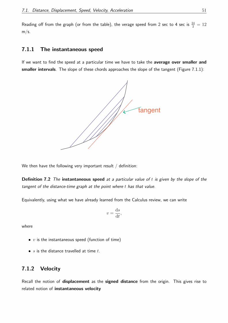
If we want to find the speed at a particular time we have to take the average over smaller and
smaller intervals. The slope of these chords approaches the slope of the tangent (Figure 7.1.1):
tangent
We then have the following very important result / definition:
Definition 7.2 The instantaneous speed at a particular value of t is given by the slope of the
tangent of the distance-time graph at the point where t has that value.
Equivalently, using what we have already learned from the Calculus review, we can write
v =ds
dt,
where
• v is the instantaneous speed (function of time)
• s is the distance travelled at time t.
7.1.2 Velocity
Recall the notion of displacement as the signed distance from the origin. This gives rise to
related notion of instantaneous velocity

52 Chapter 7. Kinematics of a particle
Definition 7.3 The instantaneous velocity is the rate of change of the displacement with respect
to time.
Equivalently, it is the speed with directional information.
Example: A particle moves at constant speed but its displacement-time graph has the following
characteristics:
Time (s) 0 2 5 6 9 10 12
Displacement from Origin 0 +4 -2 0 -6 -4 -8
Draw the displacement-time graph.
Solution – Figure 7.1.2
1 2 3 4 5 6 7 80
-1
-2
-3
-4
-5
-6
-7
-8
1
2
3
4
1211109time(s)
displacement(m)
• Particle travels 4 m in 2 seconds.
• Speed is 2 m/s, and is constant!
• But Slope of graph is ±2 – Velocity alternates between +2 and −2.
• A change in the velocity is called acceleration.
7.1. Distance, Displacement, Speed, Velocity, Acceleration 53
Definition 7.4 The instantaneous acceleration is the rate of change of velocity with respect to
time:
a =dv
dt, (7.1)
where v is the velocity.
• If a > 0 then the velocity is increasing – ‘speeding up’.
• If a < 0 then the velocity is decreasing – ‘slowing down’. Sometimes a negative acceleration
is called deceleration.
Also,
• Units of acceleration are therefore units of velocity divided by units of time.
• We write this as m/s2 and we say this is ‘metres per second per second’ or ‘metres per second
squared’.
• The slope of a velocity-time plot tells us the acceleration.
Generally, the acceleration will depend on time. However, there is a very nice mathematical theory
of kinematics for the case of constant acceleration, which we study below. We first of all have a
look at some examples.
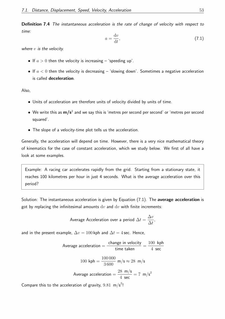
Example: A racing car accelerates rapidly from the grid. Starting from a stationary state, it
reaches 100 kilometres per hour in just 4 seconds. What is the average acceleration over this
period?
Solution: The instantaneous acceleration is given by Equation (7.1). The average acceleration is
got by replacing the infinitesimal amounts dv and dv with finite increments:
Average Acceleration over a period ∆t =∆v
∆t,
and in the present example, ∆v = 100 kph and ∆t = 4 sec. Hence,
Average acceleration =change in velocity
time taken=
100 kph
4 sec
100 kph =100 000
3 600m/s ≈ 28 m/s
Average acceleration =28 m/s
4 sec= 7 m/s2
Compare this to the acceleration of gravity, 9.81 m/s2!

54 Chapter 7. Kinematics of a particle
O
A
B
C
I II III
time(secs)
spee
d(m
/s)
17
20 40 60 80 100
5
10
15
20
E F
Example: A particle moves in the positive direction and has the velocity-time curve shown in
Figure 7.1.2. Compute the (constant) acceleration in each of the phases I, II, and III.
Solution:
• Phase I: The speed increases from 0 to 12 m/s in 40s. The acceleration = 1240
= 0.3 m/s2.
The slope of OA = 1240
= 0.3.
• Phase II: The speed increases form 12m/s to 17m/s. The acceleration = 520
= 0.25 m/s2.
The slope of AB = 520
= 0.25.
• Phase III: The speed decreases from 17 m/s to 0 m/s in 32 s. The deceleration = 1732
=
0.53 m/s2.
7.2. Mathematical description of kinematics with constant acceleration 55
7.2 Mathematical description of kinematics with constant
acceleration
time
velo
city
t
u
v
O
t
v - u
A
B
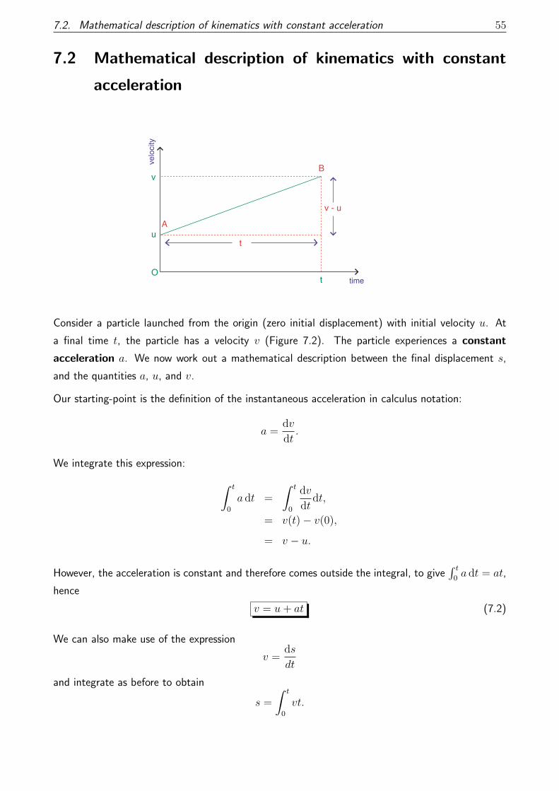
Consider a particle launched from the origin (zero initial displacement) with initial velocity u. At
a final time t, the particle has a velocity v (Figure 7.2). The particle experiences a constant
acceleration a. We now work out a mathematical description between the final displacement s,
and the quantities a, u, and v.
Our starting-point is the definition of the instantaneous acceleration in calculus notation:
a =dv
dt.
We integrate this expression: ∫ t
0
a dt =
∫ t
0
dv
dtdt,
= v(t)− v(0),
= v − u.
However, the acceleration is constant and therefore comes outside the integral, to give∫ t
0a dt = at,
hence
v = u+ at (7.2)
We can also make use of the expression
v =ds
dt
and integrate as before to obtain
s =
∫ t
0
vt.

56 Chapter 7. Kinematics of a particle
Use the expression (7.2) in the integrand here:
s =
∫ t
0
(u+ at) dt.
Hence,
s = ut+ 12at2. (7.3)
It is sometimes useful to work with expressions that do not involve t. We can eliminate t between
Equations (7.2) and (7.3) by taking Equation (7.2) and writing
t =v − ua
.
Substitute into Equation (7.3):
s = ut+ 12at2,
= u
(v − ua
)+ 1
2
(v − ua
)2
,
=uv − u2 + 1
2v2 − uv + 1
2v2
a.
Hence,
as = 12
(v2 − u2
).
Tidy up to obtain
v2 = u2 + 2as. (7.4)
7.2. Mathematical description of kinematics with constant acceleration 57
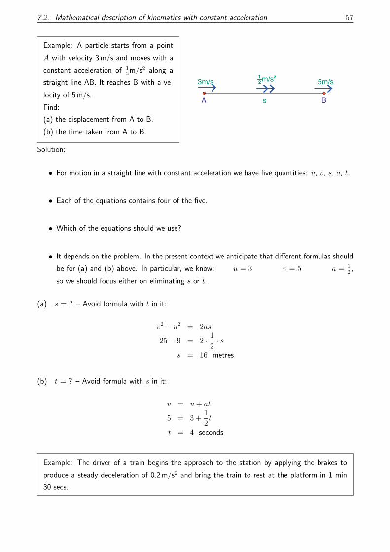
Example: A particle starts from a point
A with velocity 3 m/s and moves with a
constant acceleration of 12m/s2 along a
straight line AB. It reaches B with a ve-
locity of 5 m/s.
Find:
(a) the displacement from A to B.
(b) the time taken from A to B.
BA s
3m/s 5m/sm/s212
Solution:
• For motion in a straight line with constant acceleration we have five quantities: u, v, s, a, t.
• Each of the equations contains four of the five.
• Which of the equations should we use?
• It depends on the problem. In the present context we anticipate that different formulas should
be for (a) and (b) above. In particular, we know: u = 3 v = 5 a = 12,
so we should focus either on eliminating s or t.
(a) s = ? – Avoid formula with t in it:
v2 − u2 = 2as
25− 9 = 2 · 1
2· s
s = 16 metres
(b) t = ? – Avoid formula with s in it:
v = u+ at
5 = 3 +1
2t
t = 4 seconds
Example: The driver of a train begins the approach to the station by applying the brakes to
produce a steady deceleration of 0.2 m/s2 and bring the train to rest at the platform in 1 min
30 secs.
58 Chapter 7. Kinematics of a particle
Find:
(a) the speed when the brakes were applied,
(b) the distance travelled.
Solution: We know: t = 90, v = 0, and a = −0.2. (a) Initial speed
u = ?
v = u+ at.
0 = u− 0.2× 90.
u =2
10× 90 = 18 m/s.
(b) Distance travelled
s = ?
v2 − u2 = 2as.
0− (18)2 = 2(−0.2)s.
s = 810 m.
Example: A world-calss sprinter accelerates with constant acceleration to his maximum speed in
4.0m/s. he then maintains this speed for the remainder of a 100-m race, finishing with a total
time of 9.1s.
(a) What is the runner’s average acceleration during the first 4.0s?
(b) What is his average acceleration during the last 5.1s?
(c) What is his average accleration for the entire race?
(d) Explain why your answer to part (c) is not the average of the answers to parts (a) and (b).
Solution: It is helpful to view a velocity-versus-time plot, as in the sketch in Figure 7.3.

7.2. Mathematical description of kinematics with constant acceleration 59
Figure 7.3:
The strategy for Part (a) is to find the displacements s0 and s1 in Phases I and II in terms of the
acceleration a. In Phase I we have
s0 = 12at20,
where t0 = 4s is the duration of Phase I. In Phase II we have
s1 = v0(T − t0),
where v0 is the unknown final velocity, T = 9.1s and T − t0 = 5.1 is the duration of Phase II. The
velocity v0 and the acceleration a are connected via
a = v0/t =⇒ v0 = at0.
Combine these results to get
s0 = 12at20, s1 = at0 (T − t0) .
But
s0 + s1 = 100m,
hence12at20 + at0 (T − t0) = 100m,
hence
at0(T − 1
2t0)
= 100m.
Fill in the numbers:
a (4s) (7.1s) = 100m,

60 Chapter 7. Kinematics of a particle
hence
a = (100/28.4) = 3.5 m/s2,
correct to two significant figures.
For part (b) the velocity is constant and hence the acceleration is zero.
For part (c) the average acceleration over the whole race is
aav =vfinal − vinitial
T=v0
T= a(t0/T ).
Filling int he numbers, this is
aav = (3.52)× (4/9.1) = 1.5m/s2,
correct to two significant figures.
For part (d), a simple average of the two accelerations gives (3.5 + 0)/2 = 1.75m/s2, which is the
wrong answer. The reason this is the wrong answer is because the average should be weighted by
how much time is spent in each phase. The corrected weighted average would be
aav = a
(t0T
)+ 0
(T − t0T
)= a(t0/T ),
in agreement with the average computed in part (c).

Chapter 8
Free-fall motion under gravity
Overview
Galileo showed that all falling objects accelerate towards the Earth at a rate g that is independent
of their mass, with
g ≈ 9.81 m/s2. (8.1)
This means that we can solve simple problems involving falling objects using the formulae from the
last chapter.
61

62 Chapter 8. Free-fall motion under gravity
8.1 Calculations
In a later chapter we will give a theoretical underpinning to Equation (8.1). However, in the present
chapter we simply use the equation as-is.
Example: A brick is dropped from a scaffold
board and hits the ground 3 secs later. Find
the height of the scaffold.
h=-s
u=0
v
-9.8m/s2
xxxxxxxxxxxxxxxxxxxxxxxxxxxxxxxxxxxxxxxxxxxxxxxxxxxxxxxxxxxxxxxxxxxxxxxxxxxxxxxxxxxxxxxxxxxxxxxxxxxxxxxxxxxxxxxxxxxxxxxxxxxxxxxxxxxxxxxxxxxxxxxxxxxxxxxxxxxxxxxxxxxxxxxxxxxxxxxxxxxxxxxxxxxxxxxxxxxxxxxxxxxxxxxxxxxxxxxxxxxxxxxxxxxxxxxxxxxxxxxxxxxxxxxxxxxxxxxxxxxxxxxxxxxxxxxxxxxxxxxxxxxxxxxxxxxxxxxxxxxxxxxxxxxxxxxxxxxxxxxxxxxxxxxxxxxxxxxxxxxxxxxxxxxxxxxxxxxxxxxx
positive
xxxxxxxxxx
Solution: We know: t = 3, u = 0, and a = g. Hence,
s = ut+1
2at2
= 0× 3− 1
2× 9.8× 9
= −44.1
Thus,
h = 44.1 metres.
Example: A boulder slips from the top of a
precipice and falls vertically downwards to a
plain 200m below.
Find the speed when the boulder hits the
plain:
(a) In a polar region where g=9.830 m/s2.
(b) In an equatorial region where
g=9.781 m/s2.
s=0 u=0
s=-200
-g
Solution: We have
v2 = u2 + 2as
= 0 + 2(−g)(−200)
= 400g,
thus v = 20√g. We now fill in the specific values for g at the different locations on the earth’s
8.1. Calculations 63
surface:
(a) g = 9.830 m/s2 and v = 62.7 m/s.
(b) g = 9.781 m/s2 and v = 62.5 m/s.
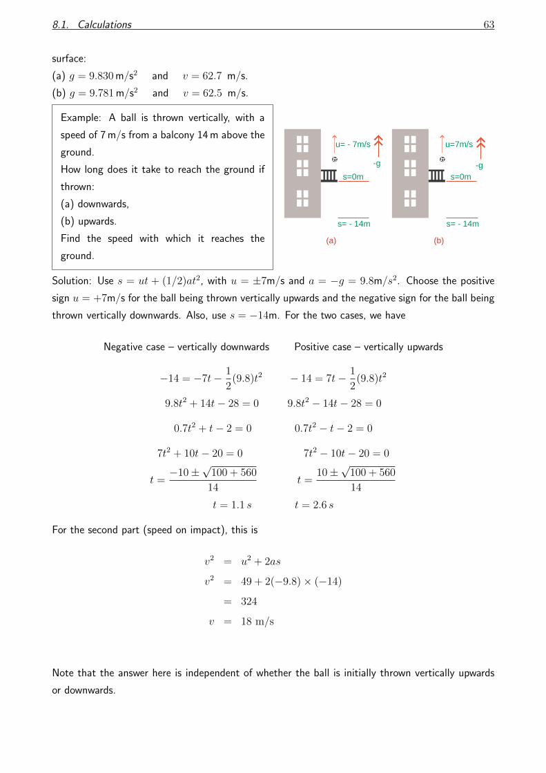
Example: A ball is thrown vertically, with a
speed of 7 m/s from a balcony 14 m above the
ground.
How long does it take to reach the ground if
thrown:
(a) downwards,
(b) upwards.
Find the speed with which it reaches the
ground.
s=0m
s= - 14m
-g
u= - 7m/s
(a)
s=0m
s= - 14m
-g
u=7m/s
(b)
Solution: Use s = ut + (1/2)at2, with u = ±7m/s and a = −g = 9.8m/s2. Choose the positive
sign u = +7m/s for the ball being thrown vertically upwards and the negative sign for the ball being
thrown vertically downwards. Also, use s = −14m. For the two cases, we have
Negative case – vertically downwards Positive case – vertically upwards
−14 = −7t− 1
2(9.8)t2 − 14 = 7t− 1
2(9.8)t2
9.8t2 + 14t− 28 = 0 9.8t2 − 14t− 28 = 0
0.7t2 + t− 2 = 0 0.7t2 − t− 2 = 0
7t2 + 10t− 20 = 0 7t2 − 10t− 20 = 0
t =−10±
√100 + 560
14t =
10±√
100 + 560
14
t = 1.1 s t = 2.6 s
For the second part (speed on impact), this is
v2 = u2 + 2as
v2 = 49 + 2(−9.8)× (−14)
= 324
v = 18 m/s
Note that the answer here is independent of whether the ball is initially thrown vertically upwards
or downwards.

Chapter 9
Forces and Newton’s first two laws of
motion
Overview
We have already described motion in kinematic terms, discussing ideas about velocity and accelera-
tion. Understanding what causes such motion requires a deeper theory, called dynamics. Basically,
forces cause motion. In this section we introduce the notion of force - first in a qualitative way and
then in a rigorous mathematical framework, which requires the introduction of Newton’s laws of
motion. We discuss Newton’s first two laws of motion, postponing discussion of the third law until
the next chapter.
64

9.1. Forces 65
9.1 Forces
Definition 9.1 Force is that which changes or tends to change the state of rest or uniform motion
of a body in a straight line.
The SI unit of force is the Newton – we will define this unit precisely in what follows. Also, force
is a vector – it has magnitude and direction.
On a fundamental level in physics there are only four forces and they are
• gravitational
• electromagnetic
• weak nuclear force
• strong nuclear force
However, such brutally elegant simplicity has no place in the kind of macroscopic world that we deal
with here, wherein we are concerned with the dynamics and statics of “large” objects. If I fall off a
ladder unharmed the first thing I do is check if the base of the ladder was secure. I do not worry
about the weak nuclear force in the constituent atoms and molecules of the ladder. Therefore, for
applications in the macroscopic world around us, we classify forces differently (but on a fundamental
level, perfectly equivalently), in the following way:
• Attraction – mainly gravitational attraction.
• Weight
• Contact forces
• Attachment
9.1.1 Gravitational attraction
Definition 9.2 The mass of a body is the quantity of matter that it contains.
Newton’s law of gravitation states the following:
Any two bodies in the universe attract each other with a force that is directly proportional
to the product of their masses and inversely proportional to the square of the distance
between them.
66 Chapter 9. Forces and Newton’s first two laws of motion
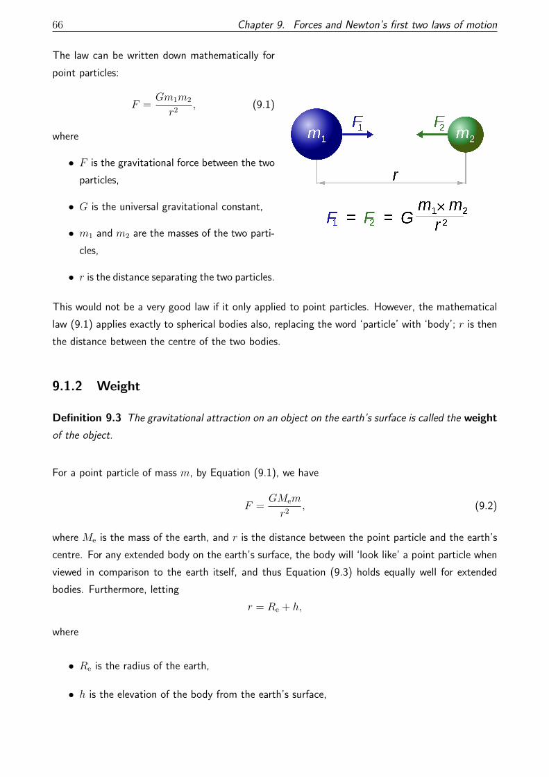
The law can be written down mathematically for
point particles:
F =Gm1m2
r2, (9.1)
where
• F is the gravitational force between the two
particles,
• G is the universal gravitational constant,
• m1 and m2 are the masses of the two parti-
cles,
• r is the distance separating the two particles.
This would not be a very good law if it only applied to point particles. However, the mathematical
law (9.1) applies exactly to spherical bodies also, replacing the word ‘particle’ with ‘body’; r is then
the distance between the centre of the two bodies.
9.1.2 Weight
Definition 9.3 The gravitational attraction on an object on the earth’s surface is called the weight
of the object.
For a point particle of mass m, by Equation (9.1), we have
F =GMem
r2, (9.2)
where Me is the mass of the earth, and r is the distance between the point particle and the earth’s
centre. For any extended body on the earth’s surface, the body will ‘look like’ a point particle when
viewed in comparison to the earth itself, and thus Equation (9.3) holds equally well for extended
bodies. Furthermore, letting
r = Re + h,
where
• Re is the radius of the earth,
• h is the elevation of the body from the earth’s surface,
9.1. Forces 67
we see that h � Re and thus, r = Re is a good approximation and finally, Equation (9.3) can be
well approximated by
F =
(GMe
R2e
)m. (9.3)
We identify GMe/R2e as a constant independent of the body in question. Indeed, we shall later be
able to demonstrate that g, the gravitational acceleration of Chapter 8 is expressed in fundamental
terms as
g =GMe
R2e
.
Thus, the force F of the earth’s gravity on the body can be written as
F = mg.
This is the object’s weight, sometimes denoted by W :
W = mg.
Caution! Mass should not be confused with weight.

68 Chapter 9. Forces and Newton’s first two laws of motion
9.2 Contact forces
These are best understood in the context of an example – see Figure 9.1.
R Reaction
W Weight
P Push F Friction
Figure 9.1: Contact forces and other forces exerted on a book
When a book is resting on a table, the table exerts a normal reaction force on the book, which is
equal to the book’s own weight. When the table is rough a frictional force acts on the book when
we slide it across the table. This acts along the surface of contact and in a direction opposing the
(potential) motion of the body.
9.2.1 Forces of attachment
Ropes, strings, etc.
T Tension
W Weight
9.3 The resultant force and force diagrams
Definition 9.4 The resultant force or net force acting on a body is the vector sum of all forces
acting on the body.

9.3. The resultant force and force diagrams 69
In symbols, the resultant force is R, and
R = F1 + F2 + · · · =∑
F .
Recall, force is a vector quantity. In what follows, it will be very useful to add up all of the forces
acting on a body using vector addition. Of course, the parallelogram law is the basis of vector
addition. But it can sometimes be helpful to represent the process of adding up all the forces by
using what is called a force diagram. The vector sum of all the forces acting on a body is called
the net force, or the resultant. The rules of force diagrams are:
1. Weight acts vertically downwards
2. Reaction is normal to surface (smooth surface)
3. If surface is not smooth there is a frictional force.
4. Attachment forces act at the point of attachment.
Two very qualitative examples of force diagrams are shown below.
Example: A block sliding down a smooth
inclined plane:
xxxxxxxxxxxxxxxxxxxxxxxxxxxxxxxxxxxxxxxxxxxxxxxxxxxxxxxxxxxxxxxxxxxxxxxxxxxxxxxxxxxxxxxxxxxxxxxxxxxxxxxxxxxxxxxxxxxxxxxxxxxxxxxxxxxxxxxxxxxxxxxxxxxxxxxxxxxxxxxxxxxxxxxxxxxxxxxxxxxxxxxxxxxxxxxxxxxxxxxxxxxxxxxxxx
W
R
NB: smooth = no friction
Example: A block pulled along a rough
horizontal surface by a rope at 50◦ to the
surface:
W
T
F
R
xxxxxxxxxxxxxxxxxxxxxxxxxxxxxxxxxxxxxxxxxxxxxxxxxxxxxxxxxxxxxxxxxxxxxxxxxxxxxxxxxxxxxxxxxx
50o

70 Chapter 9. Forces and Newton’s first two laws of motion
Example: Three customers are fighting over
the same coat in the Christmas sales. They
apply the three horizontal forces to the coat
that are shown in the figure, where the coat
is located at the origin. Find the net force on
the coat in terms of its x- and y-components.
Hence, find the magntiude and direction of the
net force.
All units are SI. Hence, the units of force are
the Newton – to be elaborated upon below.
Solution: Call the vector forces F1, F2, and F3. We resolve the forces along the Cartesian axes:
F1 = (200N) (cos 30◦i + sin 30◦j) ,
F3 = (300N) (− cos 45◦i + sin 45◦j) ,
F3 = (155N) (− cos 53◦i− sin 53◦j) .
These work out as follows:
F1 = (173i + 100j)N,
F3 = (−212i + 212j)N,
F3 = (−93i− 124j)N.
The results here are correct to three significant figures, which is the precision of the given forces in
the question.
Do the vector sum:
F1 + F2 + F3 = (173i + 100j)N
+(−212i + 212j)N,
+(−93i− 124j)N,
= [(173− 212− 93)i + (100 + 212− 124)j] N,
= (−132i + 188j)N.
This is the resultant force, R. We have
|R| =√
1322 + 1882 = 230N.

9.4. Newton’s first law 71
The angle that the resultant force makes with the x-axis is θ, where
tan θ =Ry
Rx
= −188
132=⇒ θ = − tan−1 188
132= −55◦ + · · · ,
where the inverse tangent is defined only up to a shift of an integer multiple of 180◦, and where the
angle is given to two significant figures, which is the precision given for the angles in the question.
Clearly, since Rx < 0 and Ry > 0 the resultant is in the second quadrant, hence
θ = −55◦ + 180◦ = 125◦.
9.4 Newton’s first law
Equipped with the notion of net force, we can write down Newton’s first law:
A body acted on by no net force moves with constant velocity (which may be zero) and
zero acceleration.
Equivalently, we say that a body is in equilibrium if the vector sum of forces on the body is zero:
∑F = 0 (body in equilibrium)
Therefore, by Newton’s third law, a body in equilibrium must either be at rest or be moving in a
straight line with constant velocity. We also have the following further consequences of the first
law:
• If body is at rest or moving with constant velocity in a straight line then there is no net force
on it.
• If the speed is changing, there must be a net force on the body.
The following third point is sometimes not picked up on by students on a first glance at this theory:
• If the direction of motion is changing then there must be a resultant force on the body.
In particular, this means that a particle moving in a circle experiences a net force (circular motion).
Caution! In the above presentation, we are assuming that the body can be represented adequately
as a point particle. When the body has finite size, we also have to consider where on the body
the forces are applied. This will require us to generalize the notion of equilibrium – an extended
72 Chapter 9. Forces and Newton’s first two laws of motion
body is in equilibrium if (i) the net force on the body is zero and (ii) the net moment of the
forces is zero. We will return to this topic later in th emodule.
Example: In the classic 1950 science fiction movie Rock-
etship X-M, a spaceship is moving in the vacuum of outer
space, far from any planet, when its engine dies. As a
result, the spaceship slows down and stops. What does
Newton’s first law say about this event?
Solution: In this situation, there are no forces acting on the spaceship, so according to Newton’s
first law, it will not stop. It continues to move in a straight line with constant speed. This example
of science fiction contains more fiction than science!
Example: A particle of weight 7N is hanging at the end
of a light vertical string. Find the tension in the string.
What is the tension in the string if the particle is moving
upwards with constant velocity 9.81 m/s?
T
7N
i
j
Solution:
R = (T − 7)j0,
T = 7 N.
For the second part, the particle moves with a constant velocity. This does not affect the force
balance, so the tension is still 7 N.

9.4. Newton’s first law 73
Example: Refer to the figure. A
particle rests on a rough plane in-
clined at an angle 30◦ to the hori-
zontal. Compute the friction and re-
action force experienced by the par-
ticle. Leave your answer in terms of
the particle’s weight W .
Solution: the particle is at rest, so the resultant force is zero. It remains therefore to compute the
resultant force. A coordinate system is set up as shown, such that
• Reaction force N j
• Friction force F i. The friction force can carry any sign here, and its definite value will be fixed
in the course of the calculation. So it doesn’t matter if you can’t figure out which direction
this should point in (so long as it is parallel to the plane)!
It remains to write down the gravitational force on the particle in terms of the chosen coordinate
system:
W = −W sin 30◦i−W cos 30◦j
= −1
2W i−
√3
2W j. 30
601
2
So adding the three forces together gives
Resultant R = (F − 1
2W )i + (N −
√3
2W )j.
But R = 0, hence
F = 12W, N =
√3
2W.
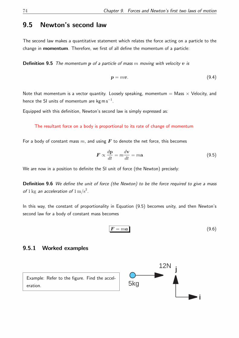
74 Chapter 9. Forces and Newton’s first two laws of motion
9.5 Newton’s second law
The second law makes a quantitative statement which relates the force acting on a particle to the
change in momentum. Therefore, we first of all define the momentum of a particle:
Definition 9.5 The momentum p of a particle of mass m moving with velocity v is
p = mv. (9.4)
Note that momentum is a vector quantity. Loosely speaking, momentum = Mass × Velocity, and
hence the SI units of momentum are kg m s−1.
Equipped with this definition, Newton’s second law is simply expressed as:
The resultant force on a body is proportional to its rate of change of momentum
For a body of constant mass m, and using F to denote the net force, this becomes
F ∝ dp
dt= m
dv
dt= ma (9.5)
We are now in a position to definite the SI unit of force (the Newton) precisely:
Definition 9.6 We define the unit of force (the Newton) to be the force required to give a mass
of 1 kg an acceleration of 1 m/s2.
In this way, the constant of proportionality in Equation (9.5) becomes unity, and then Newton’s
second law for a body of constant mass becomes
F = ma (9.6)
9.5.1 Worked examples
Example: Refer to the figure. Find the accel-
eration. 5kg
12N
i
j

9.5. Newton’s second law 75
Solution:
5a = 12i
a =12
5i = 2.4i
Acceleration = 2.4 m/s2 in the i direction.
Example: Forces 4i− 7j N and −i + 3j N act on a particle of mass 2kg.
Find the acceleration and the angle that it makes with i.
Solution: The net force is
F = (4i− 7j) + (−i + 3j) = 3i− 4j.
By Newton’s second law, F = ma. The mass is 2 kg. Hence,
F = 3i− 4j = 2a,
hence
a =1
2(3i− 4j) = 1.5i− 2j.
The angle with i is θ, where
i · a = |a| cos θ.
We have
i · a = 32, |a| =
√94
+ 4 =√
254
= 52,
hence
cos θ =i · a|a|
=3/2
5/2= 3
5,
hence
θ = cos−1 35.
Example: A rope with a bucket attached to the end is used to raise water from a well. The
mass of the empty bucket is 1.2 kg and it can raise 10 kg of water when full.
Find the tension in the rope when
(a) the empty bucket is lowered with an acceleration of 2 m/s2,
(b) the full bucket is raised with an acceleration of 0.3 m/s2.
76 Chapter 9. Forces and Newton’s first two laws of motion
Solution: For part (a), we have
• Mass: 1.2 kg
• Acceleration: a = −2jm/s2
• Weight: W = −(1.2× 9.8j) N = −11.76jN
• Tension: T = +T j, with T to be determined.
Assemble Newton’s second law for the problem:
ma = σF = W + T ,
(1.2 kg)× (−2jm/s2) = −11.76jN + T j.
Dropping the dimensional notation for now, this is
−2.4j = (−11.76 + T )j,
or
(−2.4 + 11.76− T )j = 0.
Since j is not the zero vector, the only way for this expression to hold is if
(−2.4 + 11.76− T ) = 0,
i.e. T = 9.36. Restoring the dimensions, this is T = 9.4 N, keeping two significant figures.
For (b) we have we have
• Mass: 11.2 kg
• Acceleration: a = +0.3jm/s2
• Weight: W = −(11.2× 9.8j) N = −108.76jN
• Tension: T = +T j, with T to be determined.
Assemble Newton’s second law for the problem:
ma = F = W + T ,
(11.2 kg)× (0.3jm/s2) = −108.76jN + T j.

9.5. Newton’s second law 77
Dropping the dimensional notation for now, this is
3.36j = (−108.76 + T )j,
We skip straight to the solution
3.36 + 108.76 = T,
hence
T = 112.12 N.
Example: A block of mass 4 kg is lying on the floor of
a lift that is accelerating at 5 m/s2. Find the normal
reaction exerted on the block by the lift floor if the lift
is
(a) going up,
(b) going down.
a=5R
4g
a=-5R
4g
Solution: For (a) we have
• Mass: 4 kg, acceleration +5jm/s2, ma = 20jN.
• Weight: W = −4× 9.8 = −39.2jN
• Reaction: Rj
Newton’s second law:
ma = W +Rj,
hence
20 = −39.2 +R,
hence
R = 59.2 N.
For (b) we have
• Mass: 4 kg, acceleration −5jm/s2, ma = −20jN.
• Weight: W = −4× 9.8 = −39.2jN
• Reaction: Rj
Newton’s second law:
ma = W +Rj,

78 Chapter 9. Forces and Newton’s first two laws of motion
hence
−20 = −39.2 +R,
hence
R = 19.2 N.
Example: A truck is being pulled along a
horizontal track by two cables against resis-
tances totalling 1100N with an acceleration
of 0.8 m/s2. One cable is horizontal and the
other is inclined at 40◦ to the track. The ten-
sions in the cable are as shown. Find
(a) the mass of the truck,
(b) the vertical force of the track on the truck.
R
1100N 800N
mg
i
j1000N
40o
Solution: The acceleration is in the x-direction only, so we compute the net force in the x direction,
which is
Fx = −1100 + 800 + 1000 cos 40◦ = 466 N.
Use Newton’s law for the x-direction:
max = Fx,
hence
max = 466 N.
But ax = 0.8 m/s2, hence
m =466 kg m/s2
0.8 m/s2 =466
0.8kg = 582.5 kg.
Newton’s law in the y-direction reads
may = Fy,
where the resultant force in the y-direction is R + 1000 sin 40◦ − mg. But ay = 0, hence R =
mg − 1000 sin 40◦, hence
R = (583 kg)× (9.8 m/s2)− 642.78 · · ·N = 5070.61 · · · N ≈ 5071 N.
9.6. Weight revisited 79
9.6 Weight revisited
Recall Equation (9.3), where we found that a body of mass m falling to the ground under the earth’s
gravitational attraction experiences a force
F =
(GMe
R2e
)m.
Neglecting air resistance, this is the only force on the body. Therefore, this is the net force. Hence,
under Newton’s second law, the body experiences an acceleration a, where
ma = F =
(GMe
R2e
)m.
Crucially, m cancels on both sides of this equation now:
a =GMe
R2e
.
Hence, we have rigorously shown that a particle in the earth’s gravitational field experiences a uniform
constant acceleration of magnitude GMe/R2e , which we identify as the already-studied constant g:
g =GMe
R2e
.
Therefore, the weight of the body can be written as
W = mg =GMem
R2e
.

Chapter 10
Newton’s third law of motion
Overview
We complete our discussion of Newton’s laws of motion by introducing the Third Law. We show
how this can be linked to the principle of conservation of momentum.
80

10.1. Newton’s third law – motivation and definition 81
10.1 Newton’s third law – motivation and definition
So far we have discussed the resultant force and acceleration on one particular body in any given
problem. However, particles interact with each other (by exerting forces!) and we need a principle
which describes this interaction. This is provided by Newton’s Third Law.
Action and Reaction are equal and opposite. If a body A exerts a force on a body B
then B exerts an equal and opposite force on A.
Some examples are shown in Figure 10.1.
R
R
(a) Scales pan: the pan exerts a downward force
(weight) on the scales; the scales exert an equal and
opposite upward force on the pan (reaction)
T SST
(b) Pulley: if the pulley is smooth then T = S
TT(c) Two bodies connected by a string
Figure 10.1:

82 Chapter 10. Newton’s third law of motion
10.1.1 Discussion
The Earth’s gravity exerts a force mg on a football (pulling it “down”). The football exerts exactly
the same force on the Earth (pulling it “up”). But we have Newton’s law for the earth,
Mea = F = mg
which mean’s that the earth accelerates towards the football! Why don’t we observe the earth’s
acceleration in practice?
The reason of course is that the acceleration is tiny:
a =m
Me
g.
The ball’s mass should be approximately 1 kg, the earth’s mass is approximately 1024 kg, and accel-
eration due to gravity is approximately 10 m/s2, so the acceleration will be
a = 10−23 m/s2,
which is tiny! In this case the earth’s large mass appears as inertia – the ability of the body in
question to resist changes in its motion.
10.2 Worked examples
Example: A light inextensible string passes
over a smooth pulley and carries particles of
masses 5 kg and 7 kg. If the system is moving
freely find:
(a) the acceleration of each particle,
(b) the tension in the string,
(c) the force exerted by the string on the pul-
ley.
T TTT -aa
7g5g
A B
Solution: Every word in the problem matters. So, ‘light’ means the string’s inertia can be neglected,

10.2. Worked examples 83
‘inextensibile’ means the string is totally rigid, so the force of one of the particles is transmitted
perfectly to the other. Finally, ‘smooth’ means that the tensions on both sides of the pulley are
the same – as shown in the figure. Therefore, the force balance for the two particles is rather
straightforward. Finally, the acceleration of the two particles is equal and opposite (otherwise there
would be acceleration in the string).
We first of all guess that the heavier particle B is moving downwards, and hence has an acceleration
−a. This is not necessary, as the maths will pick the sign of the acceleration – all that matters is
that the accelerations should be equal and opposite. But we have to start somewhere. Therefore,
the force balance for particle B,
−7a = T − 7g.
Similarly, for the lighter particle (particle A):
5a = T − 5g
We eliminate T between these simultaneous equations by subtracting one from the other:
−7a = T − 7g,
5a = T − 5g,
hence
12a = 2g,
hence a = g/6. The tension can be found by backsubstitution into (say) the second equation:
5a = T − 5g,
56g = T − 5g,
56g + 5g = T,
hence
T = 356g.
For (c), the total force on the pulley is the sum of
1. The tension T exerted by mass A on the pulley (downward direction)
2. The tension T exerted by mass B on the pulley (downward direction),
hence the force is 2T , or (35/6)g, in a downwards direction.

84 Chapter 10. Newton’s third law of motion
Example: A small block of mass 6 kg rests ona tabletop and is connected by a light inextensible
string that passes over a smooth pulley, fixed on the edge of the table, to another block of 5 kg
which is hanging freely.
Find the acceleration of the system and the tension in the string
(a) if the table is smooth,
(b) if the table is rough and the frictional force is 2gN.
Solution: A force diagram is shown in Figure 10.2.
xxxxxxxxxxxxxxxxxxxxxxxxxxxxxxxxxxxxxxxxxxxxxxxxxxxxxxxxxxxxxxxxxxxxxxxxxxxxxxxxxxxxxxxxxxxxxxxxxxxxxxxxxxxxxxxxxxxxxxxxxxxxxxxxxxxxxxxxxxxxxxxxxxxxxxxxxxxxxxxxxxxxxxxxxxxxxxxxxxxxxxxxxxxxxxxxxxxxxxxxxxxxxxxxxxxxxxxxxxxxxxxxxxxxxxxxxxxxxxxxxxxxxxxxxxxxxxxxxxxxxxxxxxxxxxxxxxxxxxxxxxxxxxxxxxxxxxxxxxxxxxxxxxxxxxxxxxxxxxxxxxxxxxxxxxxxxxxxxxxxxxxxxxxxxxxxxxxxxxxxxxxxxxxxxxxxxxxxxxxxxxxxxxxxxxxxxxxxxxxxxxxxxxxxxxxxxxxxxxxxxxxxxxxxxxxxxxxxxxxxxxxxxxxxxxxxxxxxxxxxxxxxxxxxxxxxxxxxxxxxxxxxxxxxxxxxxxxxxxxxxxxxxxxxxxxxxxxxxxxxxxxxxxxxxxxxxxxxxxxxxxxxxxxxxxxxxxxxxxxxxxxxxxxxxxxxxxxxxxxxxxxxxxxxxxxxxxxxxxxxxxxxxxxxxxxxxxxxxxxxxxxxxxxxxxxxxxxxxxxxxxxxxxxxxxxxxxxxxxxxxxxxxxxxxxxxxxxxxxxxxxxxxxxxxxxxxxxxxxxxxxxxxxxxxxxxxxxxxxxxxxxxxxxxxxxxxxxxxxxxxxxxxxxxxxxxxxxxxxxxxxxxxxxxxxxxxxxxxxxxxxxxxxxxxxxxxxxxxxxxxxxxxxxxxxxxxxxxxxxxxxxxxxxxxxxxxxxxxxxxxxxxxxxxxxxxxxxxxxxxxxxxxxxxxxxxxxxxxxxxxxxxxxxxxxxxxxxxxxxxxxxxxxxxxxxxxxxxxxxxxxxxxxxxxxxxxxxxxxxxxxxxxxxxxxxxxxxxxxxxxxxxxxxxxxxxxxxxxxxxxxxxxxxxxxxxxxxxxxxxxxxxxxxxxxxxxxxxxxxxxxxxxxxxxxxxxxxxxxxxxxxxxxxxxxxxxxxxxxxxxx
T
TT
T
a
a
6g
5g
A
B
xxxxxx
R
2g
in (b)
Figure 10.2:
Solution – Part (a): As before, the acceleration a for particle A is written down. The force balance
for A is simply
6a = T.
The acceleration of particle B must also be a – but in the downwards direction. Thus, the force
balance for B is
−5a = T − 5g.

10.3. Conservation of momentum 85
Eliminating T beteween these equations gives
a = 511g
Back-substitution into 6a = T gives T = (30/11)g.
Part (a): The acceleration a for particle A is written down. The force balance for A is modified:
6a = T − F = T − 2g,
where the sign of the frictional force is known – it opposes the motion. The second equation (for
B) is unchanged. We therefore have simulataneous equations:
6a = T − 2g,
−5a = T − 5g.
Eliminate T by subtraction to get 11a = 3g, hence a = (3/11)g. Back-substitution into the first
equation gives
6a = T − 2g,
6(
311g)
= T − 2g,
1811g + 2g = T,
hence T = (40/11)g.
10.3 Conservation of momentum
In ‘mechanics’ a ‘system’ is one of those terms which is kept delibeately vague. Yet it can be
thought of as a collection of particles or in slightly more generality, a collection of objects. Consider
a system of n particles each with momentum pi. The total momentum of the system P is simply
the vector sum of the individual momenta:
P = p1 + p2 + · · ·pn =n∑i=1
pi.
It is of interest to study how P changes over time. We therefore differentiate it:
dP
dt=
n∑i=1
dpidt. (10.1)

86 Chapter 10. Newton’s third law of motion
We use Newton’s second law to write
dpidt
= Fi,int + Fi,ext, (10.2)
which is the total force on the ith particle, made up of internal and external contributions:
• Fi,int is the force on the ith particle due to all the other particles in the system. Let Fij denote
the force exerted on the ith particle by the jth particle, with i 6= j. Then
Fi,int =∑jj 6=i
Fij.
• Fi,ext is the force on the ith particle due to other influences, i.e. not due to the other particles,
i.e. external forces.
Thus, Equation (10.2) becomesdpkdt
=∑j
j 6=k
Fkj + Fk,ext, (10.3)
Insert Equation (10.3) into Equation (10.1):
dP
dt=
n∑k=1
dpkdt
,
Eq. (10.3)=
n∑k=1
∑j
j 6=k
Fkj + Fk,ext
,
=n∑k=1
∑j
j 6=k
Fkj
︸ ︷︷ ︸(∗)
+n∑k=1
Fk,ext.
Here’s the thing: the first complicated-looking sum here (call it (∗)) is the sum over all forces Fkj.
To enumerate all forces in this sum, we need to write down all pairs
(1, 2), (1, 3), · · · , (1, n), (2, 1), (2, 3), · · · , (2, n), · · · (n, 1), (n, 2), · · · (n, n− 1).
These pairs appear pairwise - if (1, 2) appears in the sum, then so does (2, 1). Therefore, the sum
(∗) will involve individual pairwise sums such as
F12 + F21.

10.4. Conservation of momentum – applications 87
But by Newton’s third law, this is exactly zero. Since the sum (∗) is the sum over all such pairs,
(∗) is actually zero, and thus
dP
dt=
n∑k=1
Fk,ext. (10.4)
We define a closed system:
Definition 10.1 A closed system is one where there are no external forces.
Therefore, following on from Equation (10.4), we have the following result:
Theorem 10.1 For a closed system,dP
dt= 0,
in other words, the total momentum of the system is a constant.
This is the principle of conservation of momentum. In the next section we look at some
implications and applications of this principle.
10.4 Conservation of momentum – applications
We work through some implications and applications of the principle of conservation of momentum,
re-expressed here in word form:
In a closed system, the total momentum of the system is conserved.
Here, by ‘conserved’ we mean ‘constant’, or ‘stays the same for all time.
We can in fact relax the assumption about the system being closed: if the external force is in a fixed
direction then momentum conservation will still apply – but only in a plane perpendicular to that
direction.
Example: Pool ball collisions conserve momentum in spite of the external force of gravity because
that force is perpendicular to the plane of the pool table.

88 Chapter 10. Newton’s third law of motion
10.4.1 Worked examples
Example: A three-tonne truck is moving along a track at 8 m/s towards a five tonne truck
travelling at 5 m/s on the same track.
If the trucks become coupled at impact, find the velocity at which they continue to move if
(a) they are travelling in the same direction,
(b) in opposite direction.
Solution – part (a):
8m/s 5m/s
5 tonne3 tonne
Beforem/s m/s
5 tonne3 tonne
Aftervv
1 tonne = 1000 kg.
3000× 8 + 5000× 5 = 3000× v + 5000× v
24000 + 25000 = 8000v
8v = 49 so v = 6.125 m/s.
Part (b):
8m/s 5m/s
5 tonne3 tonne
Beforem/s m/s
5 tonne3 tonne
Aftervv
3000× 8− 5000× 5 = 3000× v + 5000× v
−1000 = 8000× v
v = −1/8 = −0.125 m/s.
Example: Two particles A and B joined by a
light inextensible string are lying together on
a smooth horizontal plane. The masses of A
and B are 1 kg and 1.5 kg respectively.
A is projected away from B with speed 5m/s.
Find the speed of each particle after the string
jerks taut.
AB
5Before
v
AB
After
1.0kg
0
1.5kg 1.5kg 1.0kg
v
Solution:
1.5× 0 + 1.0× 5 = 1× v + 1.5v
5 = 2.5v
v = 2 m/s.

10.4. Conservation of momentum – applications 89
Example: A body A of mass 4 kg travelling
with velocity 4m/s collides directly with a body
B of mass 2 kg moving with velocity 1 m/s.
They coalesce on impact.
Find the velocity with which the combined
body moves.
A B
1Before
v
A B
After
4 2
4
4 2
Solution:
4× 4 + 2× 1 = 4× v + 2× v,
18 = 6v,
v = 3 m/s.
Chapter 11
Statics and Friction
Overview
We have already discussed the topic of statics briefly - without giving it a fancy name. The idea
here is to look at situations where a system is in equilibrium and to fully characterize all of the forces
acting on the system. The key of course is Newton’s second law: since the system is in equilibrium,
there is no acceleration and hence, the vector sum of the forces is zero. We also look at frictional
forces in this context. The focus is on worked examples.
90

11.1. Review 91
11.1 Review
Recall, a body is said to be in equilibrium if the vector sum of forces on the body is zero:
∑F = 0 (body in equilibrium).
By Newton’s second law, the acceleration of a body in equilibrium is zero a = 0.
Example: A particle of weight 16 N is attached to one end of a light elastic string whose other
end is fixed.
The particle is pulled aside by a horizontal force until the string is at 30◦ to the vertical.
Find the horizontal force and the tension in the string.
Solution: Draw the force diagram shown in the
figure. We have:
Resultant = P i− 16j + T sin 60◦j− T cos 60◦i
= (P − 12T )i + (−16 +
√3
2T )j
= 0.
Therefore
P − 12T = 0, −16 +
√3
2T = 0.
T = 32√3N, P = 16√
3N.
P
T
T
16
i
j
60o
30o

92 Chapter 11. Statics and Friction
11.2 Friction
Consider the schematic diagram in the Figure
showing a block on a rough table. The block is
pulled by a force P . The potential motion of the
block due to this pulling force is opposed by fric-
tion:
• If the force P is small the block will not
move.
• As the force P is increased the block will
eventually move.
• As the force P increases, the friction in-
creases to a maximum, beyond which it can-
not increase.
R
P
W
FFriction Pull
When the block is on the point of moving friction is said to be limiting. The frictional force F has
then reached its maximum value and the block is said to be in limiting equilibrium.
11.2.1 Coefficient of friction
Consider the figure on the right showing a block
in limiting equilibrium.
Definition 11.1 For a block in limiting equilib-
rium, the coefficient
µ = F/R
being the ratio of the frictional force to the reac-
tion force, is called the coefficient of friction.
R
W
F
R
R
Resultant
Resultant
In general, µ will depend on the materials of the two contact surfaces. Also, the coefficient of
friction will in general depend on whether there is relative motion between the two surfaces: in fact
there are two coefficients of friction for static friction and dynamic friction. For the moment, we
ignore this distinction.

11.3. Friction forces - properties 93
11.3 Friction forces - properties
We begin with a definition:
Definition 11.2 The result of the reaction force R and the friction force F (with F = µR) is
called the resultant contact force.
The vector sum of these two forces is
−F i +Rj,
and hence the magnitude of the resultant contact force is
magnitude =√F 2 +R2,
=õ2R2 +R2,
= Rõ2 + 1.
Definition 11.3 The angle λ between the resultant contact force and the reaction force is called
the angle of friction.
We have
tanλ =F
R=µR
R=⇒ λ = tan−1 µ.
All of the above can be summarized in the following laws of friction:
• When the surface of two objects are in rough contact, and have a tendency to move relative
to each other, equal and opposite frictional forces act, one on each of the objects, so as to
oppose the potential movement.
• Until it reaches its limiting value, the magnitude of the frictional force F is sufficient to prevent
motion.
• When the limiting value is reached, F = µR, where R is the normal reaction between the
surfaces and µ is the coefficient of friction for those two surfaces.
• For all rough contacts 0 < F ≤ µR
• If a contact is smooth µ = 0.

94 Chapter 11. Statics and Friction
11.3.1 Worked examples
Example: A block of weight 32 N is lying in
rough contact on a horizontal plane. A hori-
zontal force of P N is applied to the block until
it is just about to move the block.
(a) If P = 8, find µ.
(b) If µ = 0.4, find P .
R
P
32
R
Solution:
• Vertically: R = 32.
• Horizontally: µR = P .
• Therefore P = 32µ.
Thus,
(a) If P = 8, µ = 832
= 14.
(b) If µ = 0.4, find P = 32× 0.4 = 12.8N.
Example: Refer to the figure. A particle of
weight 8 N rests in rough contact with a plane
inclined at α to the horizontal, where tanα =
3/4. A horizontal force of P N is applied to
the particle. When P = 16 the particle is on
the point of slipping up the plane. Find µ.
R
P
8
ij
R
53
4
90 -
Solution: We have
0 = −µRi +Rj + P cosαi
−P sinαj− 8 sinαi− 8 cosαj
= (P cosα− µR− 8 sinα)i
+(R− P sinα− 8 cosα)j
P cosα− µR− 8 sinα = 0, (11.1)
R− P sinα− 8 cosα = 0. (11.2)

11.3. Friction forces - properties 95
Now, Equation (11.2) implies:
R = P sinα + 8 cosα = 16× 35
+ 8× 45
= 16 N.
Substituting into Equation (11.1):
16µ = −8 sinα + P cosα = −8× 35
+ 16× 45
= 8,
µ = 816
= 12.
Example: Repeat the previous exercise for the case where the pushing force P is weak, such
that the block is just on the verge of sliding down the plane.
Solution: In this situation, the friction force opposes the impending motion, which is down the
plane. Therefore, the friction force points up. Thus, it is simply a matter of reversing the sign of
the friction force from the previous example, by changing µR from the previous example to −µR:
P cosα + µR− 8 sinα = 0, (11.3)
R− P sinα− 8 cosα = 0. (11.4)
From Equation (11.3):45P + 1
2R− 8× 3
5= 0,
8P + 5R− 48 = 0. (11.5)
From Equation (11.4):
R− 35P − 8× 4
5= 0,
5R− 3P − 32 = 0. (11.6)
Eliminating R between Equations (11.5) and (11.6):
11P = 16, P = 1611
N.

Chapter 12
Mechanical Energy
Overview
The concept of mechanical energy is a very useful one in mechanics. In later modules you will
see that energy is a much more fundamental idea than force. We introduce a framework in which
mechanical energy can be defined. We then state the principle of conservation of mechanical
energy. This can then be used to solve lots of different problems.
12.1 Work
Definition 12.1 When an object moves through a displacement s under the action of a constant
force F , we define the amount of work done by the force as
W = F · s. (12.1)
The SI unit of work is the Joule:
Definition 12.2 The work done by a constant force of 1 N is 1 Joule if the displacement is 1 m in
the direction of the force.
More generally, when the force is not constant, then the amount of work done during an infinitesimal
displacement is
dW = F · ds
Thus, the total work done in a net displacement s is
W =
∫ s
0
F · ds. (12.2)
96

12.1. Work 97
12.1.1 Worked examples
Example: Refer to the figure. A body rest-
ing in smooth contact with a horizontal plane
moves 2.6 m along the plane under the action
of a force of 20 N. Find the work done by a
force applied:
(a) horizontally,
(b) at 60◦ to the plane.
20N
xxxxxxxxxxxxxxxxxxxxxxxxxxxxxxxxxxxxxxxxxxxxxxxxxxxxxxxxxxxxxxxxxxxxxxxxxxxxxxxxxxxxxxxxxxxxxxxxxxxxxxxxxxxxxxxxxxxxxxxxxxxxxxxxxxxxxxxxxxxxxxxxxxxxxxxxxxxxxxxxxxxxxxxxxxxxxxxxxxxxxxxxxxxxxxxxxxxxxxxxxxxxxxxxxxxxxxxxxxxxxxxxxxxxxxxxxxxxxxxxxxxxxxxxxxxxxxxxxxxxxxxxxxxxxx
20N
xxxxxxxxxxxxxxxxxxxxxxxxxxxxxxxxxxxxxxxxxxxxxxxxxxxxxxxxxxxxxxxxxxxxxxxxxxxxxxxxxxxxxxxxxxxxxxxxxxxxxxxxxxxxxxxxxxxxxxxxxxxxxxxxxxxxxxxxxxxxxxxxxxxxxxxxxxxxxxxxxxxxxxxxxxxxxxxxxxxxxxxxxxxxxxxxxxxxxxxxxxxxxxxxxxxxxxxxxxxxxxxxxxxxxxxxxxxxxxxxxxxxxxxxxxxxxxxxxxxxxxxxxxxxxx
60o
Solution – part (a):
Work done = 20× 2.6 = 52 Joules.
Part (b): Let
s = (2.6 m)i,
F = (20 N) (cos 60◦i + sin 60◦j) .
Let W = work done. We have,
W = F · s,
= [(2.6 m)i, ] · [(20 N) (cos 60◦i + sin 60◦j)] ,
= 2.6× 20 cos 60◦ J,
= 20× 2.6× 12
J,
= 26 J.
Example: Find the work done by the earth’s gravitational
force in lifting an object through a height h at constant speed. h
j
mg
Solution: F = −mgj and s = −hj (the force and the displacement are in the same direction).
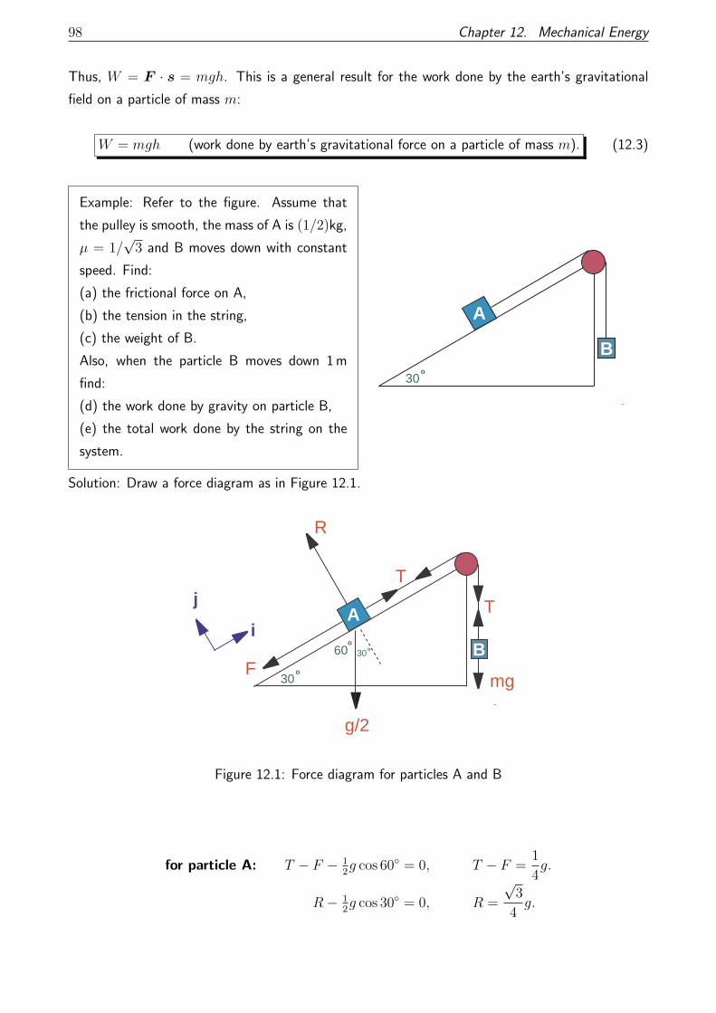
98 Chapter 12. Mechanical Energy
Thus, W = F · s = mgh. This is a general result for the work done by the earth’s gravitational
field on a particle of mass m:
W = mgh (work done by earth’s gravitational force on a particle of mass m). (12.3)
Example: Refer to the figure. Assume that
the pulley is smooth, the mass of A is (1/2)kg,
µ = 1/√
3 and B moves down with constant
speed. Find:
(a) the frictional force on A,
(b) the tension in the string,
(c) the weight of B.
Also, when the particle B moves down 1 m
find:
(d) the work done by gravity on particle B,
(e) the total work done by the string on the
system.
A
B30
o
Solution: Draw a force diagram as in Figure 12.1.
R
T
g/2
i
j
F30o
mg
TA
B60o
30o
Figure 12.1: Force diagram for particles A and B
for particle A: T − F − 12g cos 60◦ = 0, T − F =
1
4g.
R− 12g cos 30◦ = 0, R =
√3
4g.

12.2. Power 99
Thus, for part (a):
F = µR =1
4g,
and for part (b):
T = F +1
4g = µR +
1
4g =
1
4g +
1
4g =
1
2g.
For part (c) we write down the force balance for particle B, which is simply mg = T , hence mg = g/2
from Equation (12.1.1).
For part (e) the work done by the string on the particle B is due to the tension force in the string:
WT,B = (+T )× (−1 M),
while the work done by the string on the particle A is
WT,A = (+T )× (+1 M),
hence
WT,B +WT,A = 0,
and the total work done by the string on the system of two particles is zero.
As the string is totally passive in this example, it acts only to transmit the force on one particle to
the other, so we are looking at a situation in which it appears as though all work done by the string
is done directly by one particle on another through internal forces. By Newton’s third law, the sum
of all such forces is zero, and thus, the total work done by the string is zero.
12.2 Power
Definition 12.3 Power is the rate of doing work:
P =dW
dt. (12.4)
The SI unit of power is the Watt, with 1 Watt = 1Joule/second. We can also define the average
power over a finite time interval ∆t of doing work:
Paverage =Total work done in a time interval ∆t
∆t. (12.5)
100 Chapter 12. Mechanical Energy
12.3 Application – vehicle power
The power of a vehicle is defined as the rate at which the driving force is working. Suppose D is the
driving force and v is the speed. The distance moved per second is v. The Work done per second
= Dv. Therefore, the Power H of the vehicle is given by
H = Dv (12.6)
If the vehicle is stationary, H = 0
What is normally called the power of a vehicle is in fact the maximum power,
H ≡ Pmax.
Note that if a vehicle moves under its constant, maximum power Pmax and a resistance force Fres
then the equation of motion (Newton’s Second Law) is
mdv
dt= D − Fres =
Pmax
v− Fres
We’ll solve equations like this later, but for the
moment we simply note that starting from rest the
vehicle will ultimately reach a maximum velocity
(at maximum power !) given by
vmax =Pmax
Fres.

12.3. Application – vehicle power 101
Example: On a level track, a train has a max-
imum speed of 50 m/s. The total resistance is
28 kN. Find the maximum power of the engine.
DR=28000N
Solution: Start with Newtno’s second law: Newton’s Second Law:
Ma = D − Fres.
At maximum power a = 0. Therefore
D = Fres = 28,000.
But Pmax = Dvmax, hence
Pmax = Dvmax = 28,000× 50 = 1,400,000 W
= 1400 kW = 1.4 MW
Example: Following on from the previous exercise, suppose that the total resistance is reduced
and the power needed to maintain the speed at 50 m/s is now 1250 kW. Find the new resistance.
Solution: We have
Pmax = 1250 kW = Dvmax = D × (50 m/s).
ButPmax
vmax
= D =⇒ D =1250× 103
50= 25 kN.
There is no acceleration, hence Fres = D, hence
Fres = 25 kN.

102 Chapter 12. Mechanical Energy
Example: When a car of mass 1200 kg is driv-
ing up a hill inclined at an angle α to the
horizontal, with engine working at 32 kW, the
maximum speed is 25 m/s.
If α = sin−1(
116
), find the resistance to mo-
tion.R
D
Mg
Solution: There is no acceleration. Therefore, the forces are in equilibrium. A force balance in the
x-direction (i.e. in the direction along the incline) gives
D = Fres +W sinα.
But Pmax = Dvmax, hencePmax
vmax
= D,
hencePmax
vmax
= Fres +W sinα.
Re-arranging gives
Fres =Pmax
vmax
−W sinα.
Fill in the numbers:
Fres =32, 000
25− 1200× 9.1× 1
16,
= 545 N.
Example: A cyclist on a flat road moves rides at maximum power to obtain a speed of v = 8 m/s.
To maintain this speed, the cyclist must overcome two forces:
• Rolling friction due to contact with the road:
Frolling friction = µW,
where µ is the coefficient of rolling friction and W is the combined weight of the bike and
the rider.
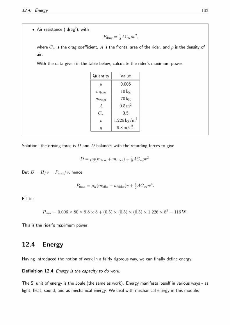
12.4. Energy 103
• Air resistance (‘drag’), with
Fdrag = 12ACwρv
2,
where Cw is the drag coefficient, A is the frontal area of the rider, and ρ is the density of
air.
With the data given in the table below, calculate the rider’s maximum power.
Quantity Value
µ 0.006
mbike 10 kg
mrider 70 kg
A 0.5 m2
Cw 0.5
ρ 1.226 kg/m3
g 9.8 m/s2.
Solution: the driving force is D and D balances with the retarding forces to give
D = µg(mbike +mrider) + 12ACwρv
2.
But D = H/v = Pmax/v, hence
Pmax = µg(mbike +mrider)v + 12ACwρv
3.
Fill in:
Pmax = 0.006× 80× 9.8× 8 + (0.5)× (0.5)× (0.5)× 1.226× 83 = 116 W.
This is the rider’s maximum power.
12.4 Energy
Having introduced the notion of work in a fairly rigorous way, we can finally define energy:
Definition 12.4 Energy is the capacity to do work.
The SI unit of energy is the Joule (the same as work). Energy manifests iteself in various ways - as
light, heat, sound, and as mechanical energy. We deal with mechanical energy in this module:
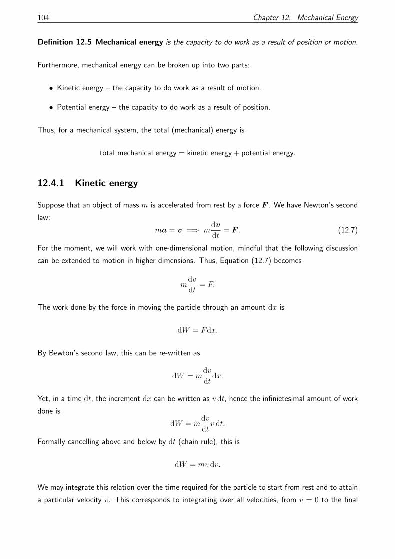
104 Chapter 12. Mechanical Energy
Definition 12.5 Mechanical energy is the capacity to do work as a result of position or motion.
Furthermore, mechanical energy can be broken up into two parts:
• Kinetic energy – the capacity to do work as a result of motion.
• Potential energy – the capacity to do work as a result of position.
Thus, for a mechanical system, the total (mechanical) energy is
total mechanical energy = kinetic energy + potential energy.
12.4.1 Kinetic energy
Suppose that an object of mass m is accelerated from rest by a force F . We have Newton’s second
law:
ma = v =⇒ mdv
dt= F . (12.7)
For the moment, we will work with one-dimensional motion, mindful that the following discussion
can be extended to motion in higher dimensions. Thus, Equation (12.7) becomes
mdv
dt= F.
The work done by the force in moving the particle through an amount dx is
dW = Fdx.
By Bewton’s second law, this can be re-written as
dW = mdv
dtdx.
Yet, in a time dt, the increment dx can be written as v dt, hence the infinietesimal amount of work
done is
dW = mdv
dtv dt.
Formally cancelling above and below by dt (chain rule), this is
dW = mv dv.
We may integrate this relation over the time required for the particle to start from rest and to attain
a particular velocity v. This corresponds to integrating over all velocities, from v = 0 to the final

12.4. Energy 105
particular velocity of interest v. ∫dW =
∫ v
0
mv dv = 12mv2. (12.8)
This is the work done in accelerating the particle from rest to a new state where the particle has
velocity v. This is work done due to motion – kinetic energy. Thus,
kinetic energy = 12mv2.
Kinetic energy is given the symbol T or K, and it is a fundamentally non-negative quantity. For
motion in higher dimensions this result generalizes to
T = 12mv2,
where v is the vector velocity and v2 = v · v.
12.4.2 Work–energy theorem
More generally, we may suppose that a particle experiences a force to accelerate it from an initial
velocity v1 to a final velocity v2, taking it from a position x1 to a final position at x2. Then,
Equation (12.8) becomes ∫ x2
x1
dW =
∫ v2
v1
mv dv = 12mv2
2 − 12mv2
1, (12.9)
which can also be written as
W (x1 → x2) = 12mv2
2 − 12mv2
1.
This result is the work-energy theorem:
The work done in moving a particle through a displacement x1 → x2 is equal to the
corresponding change in the particle’s kinetic energy.
12.4.3 Potential energy
In one dimension, Potential energy can be defined for forces that do not depend explicitly on time.
Specifically, consider again Equation (12.9) and write dW = F (x)dx. Introduce
U(x) =
∫ x
a
F (x) dx,

106 Chapter 12. Mechanical Energy
where a is some arbitrary reference level.
Definition 12.6 For a force in one dimension F (x) that does not depend explicitly on time,
U(x) = −∫ x
a
F (x) dx, (12.10)
is called the potential energy. Potential energy is defined with respect to an arbitrary reference
level a.
Definition 12.7 A force is called conservative if it has a potential-energy function along the lines
of Equation (12.10).
In one dimension, all forces that are a function only of position are obviously conservative. In higher
dimensions, things are a bit trickier. In one dimension and higher, gravity is a conservative force, as
we will demonstrate later. For a conservative force, we have
W (x1 → x2) =
∫ x2
x1
dW,
conservative force=
∫ x2
x1
F (x)dx,
=
∫ a
x1
F (x)dx+
∫ x2
a
F (x)dx,
=
∫ x2
a
F (x)dx−∫ x1
a
F (x)dx,
= −U(x2) + U(x1),Work-energy theorem
= 12mv2
2 − 12mv2
1,
Note that the precise value of the reference level a doesn’t matter here because it appears twice in
a self-cancelling way. Re-arranging these relations, we have
12mv2
1 + U(x1) = 12mv2
2 + U(x2).
Thus, the mechanical energy is the same at positions x1 and x2 and hence, at all positions. This
gives the following principle of conservation of mechanical energy:
For a conservative force F (x), the total mechanical energy
E = 12mv2 + U(x), U(x) = −
∫ x
a
F (x)dx (12.11)
is conserved.
Here, by ‘conserved’ we mean ‘constant’ or ‘not changing with time’.

12.4. Energy 107
12.4.4 Caution!
Caution: We have derived the principle of conservation of mechanical energy from (work-energy
theorem)+(conervataive forces). The work-energy theorem is therefore much more general
starting-point and holds for all forces.
The work-energy theorem holds for all forces and is very useful for solving problems - including those
involving friction, as in the following example.
Example: A small block of mass 3 kg is mov-
ing on a horizontal plane against a constant
resistance of RN. The speed of the block falls
from 12 m/s to 7 m/s as the block moves 5 m.
Find the magnitude of the resistance.
R12m/s 7m/s
5m
Solution: Use the work-energy theorem. The change in the kinetic energy is
∆T = 12m(122 − 72 m/s2) = 142.5 J.
This is equal to the work done by the resistance force on the block:
∆T =
∫Rdx = Rx = R(5 m),
hence
R =∆T
x=
142.5 J
5m= 28.5 N.
12.4.5 Gravity
The gravitational force on a particle is F = −mg (downward). This corresponds to a standard
coordinate line x where x > 0 points upward and x < 0 points downward. The potential energy
function is thus
U(x) = −∫ x
a
F dx = +mg(x− a),
where a is the reference level. Calling h = x− a, the potential energy can be written as
U(x) = mgh.
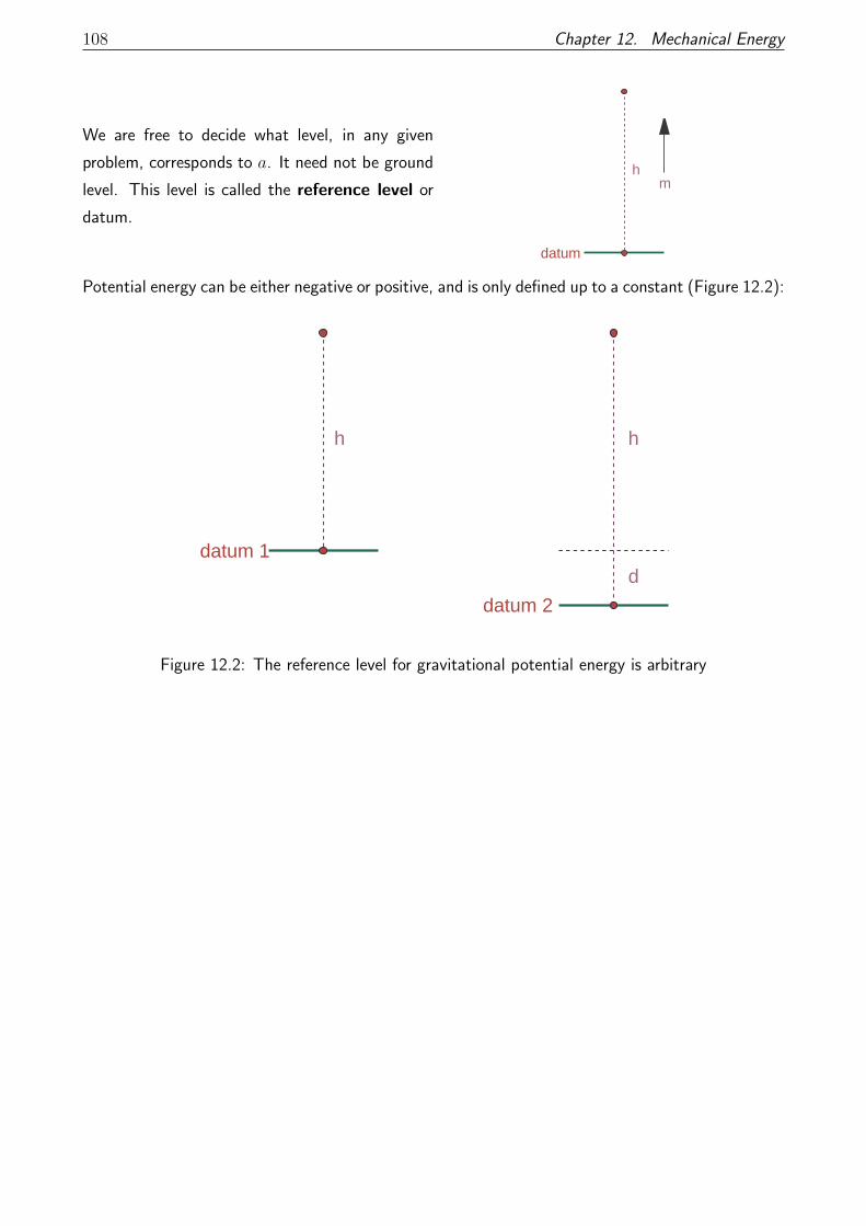
108 Chapter 12. Mechanical Energy
We are free to decide what level, in any given
problem, corresponds to a. It need not be ground
level. This level is called the reference level or
datum.
hm
datum
Potential energy can be either negative or positive, and is only defined up to a constant (Figure 12.2):
h
datum 1
h
datum 2d
Figure 12.2: The reference level for gravitational potential energy is arbitrary

12.4. Energy 109
Example: A man of 72 kg climbs up a ladder to
a height of 5 m. Assuming that the man can
be treated as a particle(!), find the potential
energy relative to the ground.
m=72kg
h=5m
Solution:
• Potential energy gained:
mgh = 72× 9.8× 5 = 3528 Joules.
• Potential energy lost:
72× 9.8× 3 = 2117 Joules.
Example: A small block A of mass 2 m is lying
in smooth contact with a table top. A light
inextensible string of length 1 m is attached at
one end to A, passes over a smooth pulley and
carries a block of mass m hanging freely at the
other end. Initially A is held at rest 0.8 m from
the edge of the table.
If the system is released, find the speed of A
when it reaches the edge.
0.2 m
20.8 m
A
B m
m
FinalInitial
1 m
2mA
B m
Solution:
• Initial mechanical energy E1 = −mg × 0.2 = −0.2mg.
• Final mechanical energy:
E2 = 12× 2m× v2 + 1
2×m× v2 −mg × 1 =
3
2mv2 −mg.

110 Chapter 12. Mechanical Energy
The mechanical energy is conserved: E1 = E2:
−0.2mg = 32mv2 −mg,
32mv2 = mg − 0.2mg,
32v2 = g − 0.2g = 0.8g,
v2 = 23× 0.8g = 5.227.
v = 2.29 m/s.
12.5 More worked examples
Example: Water is being raised by a pump
from a storage tank at ground level and ejected
at 3 m above ground level though a pipe at
6 m/s. The water is delivered at a rate of
420 kg per second.
Find the mechanical energy supplied by the
pump in one second (the power).
h=3mv=6m/s
Solution: The energy at the reference level (ground level) is unknown and equal to E1. The mass
in question is
∆m = (420 kg/sec)× 1 sec := Q∆t,
where ∆t = 1 sec and Q = 420 kg/sec. Thus, the energy at height h = 3 m is
E2 = 12∆mv2 + ∆mgh = ∆m
(12v2 + gh
).
By conservation of mechanical energy, E1 = E2 and thus,
P =E1
∆t=E2
∆t,
=∆m
(12v2 + gh
)∆t
,
= Q(
12v2 + gh
).
Filling in, this is
P = 420(
1262 + 9.8× 3
)= 19908 Joules/sec.

12.5. More worked examples 111
Example: A stone, of mass 4 kg, falls vertically
downwards through a tank of viscous oil. The
speed as the stone enters the oil is 2 m/s and,
at the bottom of the tank, it is 3 m/s. The
depth of the oil is 2.4 m.
Find the oil resistance on the stone.
R
2m/s
3m/s
2.4m
Solution: Resistance forces are a bit mysterious. They are part of a family of ‘dissipative forces’
where their functional form F = F (· · · ) is a complicated function of velocity. They are therefore
not conservative in general. Thus, we cannot assume here that energy is conserved. But we can
still use the work-energy theorem! We have
∆T =
∫Fnetds,
where the net force is mg −R, hence
12m(v2
2 − v21) = (mg −R)h,
where h = 2.4m, where the subscript 1 denotes the top of the tank, and where the subscript 2
denotes the bottom of the tank. Fill in the values:
12(4 kg)
(32 − 22 m/s2) = (mg −R)h,
hence
(mg −R)h = 10.
Thus,
R = mg − 10
h.
Fill in the numbers:
R = (4× 9.8)− (10/2.4) = 35.03 N.

112 Chapter 12. Mechanical Energy
Example: A car of mass 1000 kg drives up a
slope of length 750 m at an incline of 1 in 25. If
the resistance is negligible, calculate the driv-
ing force of the engine if the speed at the foot
of the slope is 25 m/s and the speed at the top
is 20 m/s.
Take the inclinea of 1/25 to mean
sinα = 125
.
aThis is a rather unusual example as the inclineusually refers to the tan of an angle. Because 1/25 isso small, tan(α) ≈ sin(α) ≈ α in this example, so theunusual nature of the example is not important.
RD
Mg
75030
Solution: note that there is a change in the velocities, so there is an acceleration, hence the forces
are unbalanced. A force diagram will therefore not help. Also, note that we are looking to solve for
an unknown force, so the principle of conservation of mechanical energy – although applicable – will
not help us here. The only thing to do then is to use the work-energy theorem again. We compute
the change in kinetic energy, letting the subscript 2 denote the final situation (top of hill) and the
subscript 1 denote the initial situation (bottom of hill):
∆T = 12m(v2
2 − v21) = 1
2(1000 kg)
(202 − 252 m/s2) = −112500 J.
We, err, work out the work done by the forces on the car. We split the net force into the gravitational
force and the driving force:
F = Fgrav + Fdrive.
In the standard coordinate system,
Fgrav = −mg (sinαi + cosαj) ,
Fdrive = Di,
and the displacement is s = ∆xi, with ∆x = 750 m. Thus,
W = F · s = (D −mg sinα)∆x.

12.5. More worked examples 113
We now apply the work-energy theorem:
∆T = W,
−112500 = (D −mg sinα)∆x,
mg sinα∆x− 112500 = D∆x.
Thus,
D∆x = 181, 500,
and the driving force is thus
D =181, 500
∆x=
181, 500
750= 242 N.
Chapter 13
Conservation of momentum – application
to particle collisions
Overview
We use the principles of conservation of momentum and conservation of mechanical energy to
analyse collisions between particles.
13.1 General principles
Recall in Chapter 10 we defined the momentum of a system of n particles, each its own individual
momentum pi:
(Momentum of system:) P = p1 + p2 + · · ·pn
We also showed how the principle of conservation of momentum follows from Newton’s second and
third laws:
In a closed system, the total momentum of the system is conserved,
where by ‘conserved’ we mean ‘constant’, or ‘stays the same for all time. We also relaxed the
assumption about the system being closed: if the external force is in a fixed direction then momentum
conservation will still apply – but only in a plane perpendicular to that direction.
Consider also the mechanical energy of a closed system. Because there is no net external force on
such a system, there principle of mechanical energy states that the kinetic energy will be conserved:
K.E = const (closed system).
114

13.2. Elastic collisions 115
13.2 Elastic collisions
Consider the collision shown in Figure 13.1
m mBA
u uA B
m mBA
A Bv v
AfterBefore
Figure 13.1: Elastic collision between two particles
Conservation of momentum gives
m1u1 +m2u2 = m1v1 +m2v2.
Conservation of kinetic energy gives
12m1u
21 + 1
2m2u
22 = 1
2m1v
21 + 1
2m2v
22.
Let µ = m2/m1. Then, conservation of kinetic energy reduces to
u21 + µu2
2 = v21 + µv2
2
u21 − v2
1 = µ(v22 − u2
2)
(u1 + v1)(u1 − v1) = µ(v2 + u2)(v2 − u2). (13.1)
From conservation of momentum we have m1u1 +m2u2 = m1v1 +m2v2, hence
u1 − v1 = µ(v2 − u2) (13.2)
Substitute Equation (13.2) into Equation (13.1) to obtain
v1 − v2 = −(u1 − u2).
Definition 13.1 A collision in which the kinetic energy is conserved is called elastic. In an elastic

116 Chapter 13. Conservation of momentum – application to particle collisions
collision between two bodies, the relative velocities before and after the collision are related via
v1 − v2 = −(u1 − u2). (13.3)
Note that in a closed system (no interaction between the particles and the environment) the collision
will be necessarily elastic. In contrast, in an open system, things are a bit more complicated.
13.3 Inelastic collision between two particles
In practice, collisions are inelastic: energy is transferred from the closed system to the outside
world via heat, sound, etc. However, in such scenarios, conservation of momentum still holds. We
therefore need to reformulate our conservation laws slightly to solve problems for inelastic collisions.
Therefore, for inelastic collisions, we have the following two principles:
• Conservation of momentum
• Conservation of kinetic energy Newton’s law of restitution:
(Relative speed after collision) = −CR × (Relative speed before collision)
where CR is the coefficient of restitution.
This can be thought of as a generalization of the previous analysis of elastic collisions: Newton’s
law of restitution can be thought of as a generalization of Equation (13.3), which now reads
v1 − v2 = −CR(u1 − u2). (inelastic collisions)
Note that the special case of elastic collisions can always be recovered by setting CR = 1.
13.4 Worked examples
Example: A particle A of mass 0.1 kg is moving
with velocity 2 m/s towards another particle B
of mass 0.2 kg which is at rest. Both particles
are on a smooth horizontal table. If the coef-
ficient of restitution between A and B is 0.8
find the velocity of each particle after collision.Before
v1
Afterv
2u2 = 0m/su1 = 2m/s
0.1 0.2 0.1 0.2
A B BA

13.4. Worked examples 117
Solution: Start with momentum conservation:
m1u1 +m2u2 = m1v1 +m2v2,
0.1× 2 + 0.2× 0 = 0.1× v1 + 0.2× v2,
0.2 = 0.1v1 + 0.2v2,
2 = v1 + 2v2.
We also have Newton’s law of restitution:
v1 − v2 = −CR(u1 − u2)
v1 − v2 = −0.8(2− 0)
v1 − v2 = −1.6.
These two principles therefore provide simultaneous equations in v1 and v2:
v1 + 2v2 = 2,
v1 − v2 = −1.6.
The solution:
3v2 = 3.6, v2 = 1.2
v1 = v2 − 1.6 = −0.4.
Example: A particle P of mass 1 kg, moving
with speed 4 m/s collides directly with another
particle Q of mass 2 kg moving in the opposite
direction with speed 2 m/s. The coefficient of
restitution for these particles is 0.5.
Find
(a) the velocity of each particle after collision,
(b) the loss in kinetic energy.
Beforev1
Afterv
2u2 = -2m/su1 = 4m/s
1 2 1 2
P Q QP
Solution – part (a). Use the principle of conservation of momentum:
m1u1 +m2u2 = m1v1 +m2v2,
1× 4 + 2× (−2) = 1× v1 + 2× v2,
v1 + 2v2 = 0.

118 Chapter 13. Conservation of momentum – application to particle collisions
Again, we have Newton’s law of restitution:
v1 − v2 = −CR(u1 − u2),
v1 − v2 = −0.5(4− (−2)) = −3,
v1 − v2 = −3.
We obtain two simultaneous equations:
v1 + 2v2 = 0,
v1 − v2 = −3,
with solution
3v2 = 3, v2 = 1,
v1 = v2 − 3 = 1− 3 = −2,
hence
v1 = −2 m/s, v2 = 1 m/s.
For part (b) we have
Einit = 12m1u
21 + 1
2m2u
22,
= 12× 1× 16 + 1
2× 2× 4,
= 12 J,
and
Efin = 12m1v
21 + 1
2m2v
22,
= 12× 1× 4 + 1
2× 2× 1,
= 3 J,
The loss in kinetic energy is
Einit − Efin = (12− 3)J = 9J.

13.5. Collisions with a fixed wall 119
13.5 Collisions with a fixed wall
For collisions of a particle with a fixed wall, the principle of conservation of momentum is of no use.
For example, consider a particle moving at right angles to a wall. The particle velocity changes sign
after the collision, meaning that there is a change in the particle’s momentum. Thus, the particle
experiences an external force during the collision, namely the reaction force of the wall on the
particle. In the collision, kinetic energy is not necessarily conserved either, so the only principle we
can resort to is Newton’s law of restitution. Thus, if a particle moving with speed u, perpendicular
to a wall, collides with the wall, then the velocity is reversed and the speed is CRu, where CR is
the coefficient of restitution between the wall and particle. This principle can be seen in the figure
below:
Before After
euu
[v1 − v2 = −CR(u1 − u2)] =⇒ [v1 = −CRu1]

Chapter 14
Circular motion
Overview
In this chapter, we consider a particle constrained to move in a circle.
14.1 Introduction and definitions
In this section we consider a particle constrained to move in a circle. We begin with some basic
definitions:
Definition 14.1 Angular velocity is the rate of change of θ with time:
ω =dθ
dt. (14.1)
• measured in radians/second
• Beware units: revs/sec, revs/min, revs/hr
(1 rev = 2π radians)
• We take positive θ to be in the anticlockwise
sense.
• Angular speed = |dθ/dt|
+
120
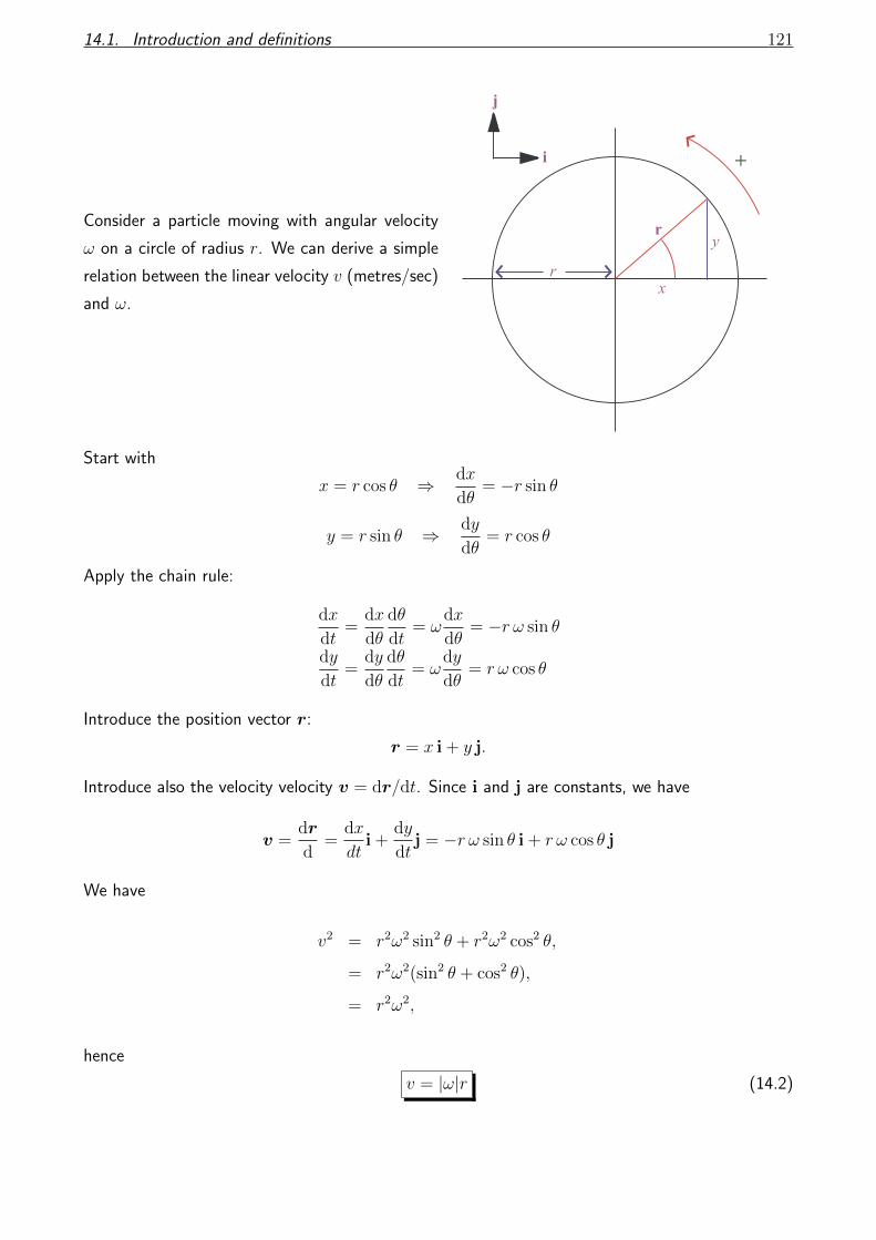
14.1. Introduction and definitions 121
Consider a particle moving with angular velocity
ω on a circle of radius r. We can derive a simple
relation between the linear velocity v (metres/sec)
and ω.
+
x
y
r
r
i
j
Start with
x = r cos θ ⇒ dx
dθ= −r sin θ
y = r sin θ ⇒ dy
dθ= r cos θ
Apply the chain rule:
dx
dt=
dx
dθ
dθ
dt= ω
dx
dθ= −r ω sin θ
dy
dt=
dy
dθ
dθ
dt= ω
dy
dθ= r ω cos θ
Introduce the position vector r:
r = x i + y j.
Introduce also the velocity velocity v = dr/dt. Since i and j are constants, we have
v =dr
d=
dx
dti +
dy
dtj = −r ω sin θ i + r ω cos θ j
We have
v2 = r2ω2 sin2 θ + r2ω2 cos2 θ,
= r2ω2(sin2 θ + cos2 θ),
= r2ω2,
hence
v = |ω|r (14.2)
122 Chapter 14. Circular motion
Example: Express
(a) 3 rev/min in rad/sec,
(b) 0.005 rad/sec in rev/hr.
Solution:
(a) 1 rev = 2π radians. 3 rev/min → 3×2π60
rad/sec = π10
rad/sec.
(b) 1 rad = 12π
rev. 0.005 rad/sec → 0.0052π× 3600 rev/hr = 9
πrev/hr.
Example: A point on the circumference of a disc is rotating at a constant speed of 3 m/s. If
the radius of the disc is 0.24 m, find in rad/sec the angular speed of the disc.
Solution:
v = 3 m/s
r = 0.24 m
v = |ω| r
Hence,
|ω| = v
r=
3
0.24= 12.5 rad/sec.
14.2 Centripetal Acceleration
When a particle follows a circular path at constant speed, the velocity vector changes with time as
the particle turns. Therefore, the particle is accelerating, even though the speed remains constant
since acceleration is the rate of change of velocity. This is known as centripetal acceleration. If
the particle also speeds up or slows down, it has an extra contribution to the acceleration known
as angular acceleration. The aim of this section is to derive a mathematical expression for the
acceleration for a particle constrained to execute circular motion.
To do this, we introduce polar coordinates. We start by introducing the concepts of unit normal
and unit tangent vectors to the circle, as shown in Figure 14.1.

14.2. Centripetal Acceleration 123
r
ni
j
t
r
Figure 14.1: The unit normal and unit tangent vectors to the circle
Referring to the figure, we see that while the unit cartesian vectors i and j are fixed, both n(t) and
t(t) are functions of time: they depend on the particle’s instantaneous position. Like any vector,
n(t) and t(t) can be written in terms of their cartesian components:
n(t) = cos θ(t) i + sin θ(t) j
t(t) = − sin θ(t) i + cos θ(t) j
A nice thing about these equations is that they can be put into matrix form:(n
t
)=
(cos θ sin θ
− sin θ cos θ
)(i
j
),
and the inverse is particularly simple: A nice thing about these equations is that they can be put
into matrix form: (i
j
)=
(cos θ − sin θ
sin θ cos θ
)(n
t
);
in particular,
j = sin θn + cos θt. (14.3)
In any case, we can now write the displacement (r), velocity (v) and acceleration (a) vectors in

124 Chapter 14. Circular motion
either Cartesian or polar coordinates.
• Displacement: We have
r = xi + yj,
= r cos θi + r sin θj,
= r(cos θi + r sin θj),
= rn.
• Velocity: We have
v = −r ω sin θ i + r ω cos θ j,
= rω(− sin θi + ω cos θj),
= rω t.
The velocity is always in the tangential direction.
We now work on the acceleration: We have
v(t) = rω t,
and
a =dv
dt.
By the product rule, we have
a = rtdω
dt+ rω
dt
dt, (14.4)
so it remains to work out dt/dt:
dt
dt=
d
dt(− sin θi + cos θj) ,
= −idθdt
d
dθsin θ + j
dθ
dt
d
dθcos θ,
= −ωi cos θ − ωj sin θ,
= −ωr.
Hence, Equation (14.4) becomes
a = rtdω
dt− rω2r.

14.2. Centripetal Acceleration 125
This is an important result, so we put it in a nice box:
a =dv
dt= rt
dω
dt− rω2r. (14.5)
Note that the radial component of the acceleration is −ω2rn which has magnitude ω2r and is
directed towards the centre of the circle:
For a particle to move in a circle, it has to have an acceleration of ω2r towards the
centre.
By Newton’s second law, there must be a net force on the particle acting towards the centre of the
circle. The magnitude of the force must be equal to mω2r. Taking Equations (14.2) and (14.5) the
acceleration towards the centre (centripetal accelaration) can also be written as
Centripetal acceleration = ω2r =v2
r. (14.6)
Caution! The expression Force = mω2r can be misleading – even if it is very simple. It seems to
state that the circular motion produces a force. This is mixing up cause and effect! Things are
the other way around. Forces must be present to constrain the particle to do circular motion.
The net result of these forces is the acceleration mω2r. The expression mω2r is an effect of the
forces. It is not the cause of the motion.
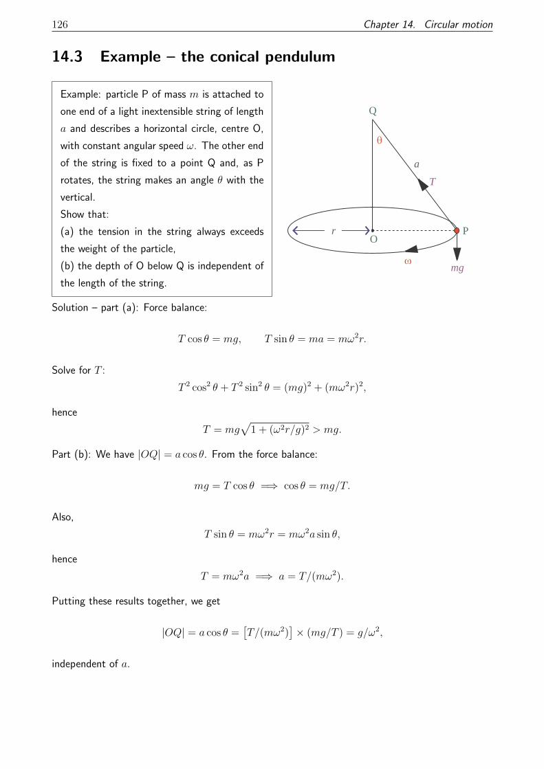
126 Chapter 14. Circular motion
14.3 Example – the conical pendulum
Example: particle P of mass m is attached to
one end of a light inextensible string of length
a and describes a horizontal circle, centre O,
with constant angular speed ω. The other end
of the string is fixed to a point Q and, as P
rotates, the string makes an angle θ with the
vertical.
Show that:
(a) the tension in the string always exceeds
the weight of the particle,
(b) the depth of O below Q is independent of
the length of the string.
PO
mg
T
r
a
Q
Solution – part (a): Force balance:
T cos θ = mg, T sin θ = ma = mω2r.
Solve for T :
T 2 cos2 θ + T 2 sin2 θ = (mg)2 + (mω2r)2,
hence
T = mg√
1 + (ω2r/g)2 > mg.
Part (b): We have |OQ| = a cos θ. From the force balance:
mg = T cos θ =⇒ cos θ = mg/T.
Also,
T sin θ = mω2r = mω2a sin θ,
hence
T = mω2a =⇒ a = T/(mω2).
Putting these results together, we get
|OQ| = a cos θ =[T/(mω2)
]× (mg/T ) = g/ω2,
independent of a.
14.4. Motion in a vertical circle 127
14.4 Motion in a vertical circle
We now consider motion in a vertical circle, and the consequence of this is that the particle speed
is not constant:
• Particles slow down as they rise on a circular path
• They speed up as they fall.
In principle, we have to write the equation of motion (Newton’s Second Law) in the tangential
direction. This allows us to solve for the angular acceleration. However, in most cases of interest,
the work done by the non-gravitational forces is zero. For example, a reaction force normal to the
circular path does no work. We then have conservation of mechanical energy:
E =1
2mv2 +mgh = constant
This, together with the radial part of the equation of motion, allows us to solve the problem.
Example: One end of a light rod of length a metres is pivoted at a fixed point O. A particle of
mass m kg is attached to the other end. The rod is hanging at rest.
The particle is given a blow and moves initially with velocity u m/s.
(a) Find the value of u if the rod comes to rest first when horizontal.
(b) Show that the particle will perform a complete circle if u > 2√ga.
(c) When u = 2√ga find the force in the rod when the particle is at the highest point.
(d) If u =√
3ga find the height of the particle above the centre of the circle when the tension
is zero.
Solution – part (a). Use conservation of mechanical energy:
Einit = 12mu2.
Where the reference level is the bottom of the circle.
Efinal = mga.
Einit = Efinal =⇒ u =√
2ga.
Part (b): Again, by conservation of mechanical energy:
12mv2 +mga(1− cosφ) = 1
2mu2,

128 Chapter 14. Circular motion
Figure 14.2: Force balance for the vertical circle
where h = a(1− cosφ) is the height above the reference level. Re-arranging gives
12mv2 = 1
2m[u2 − 2ga(1− cosφ)
].
We must have12mv2 > 0, ∀φ
hence
u2 − 2ga(1− cosφ) > 0 ∀φ.
In the worst-case scenario (φ = π, cosφ = −1), we must have
u2 − 4ga > 0,
hence
u > 2√ga.
Part (c): When u = 2√ga at the top of the circle, the particle is just barely doing circular motion. It
follows that the net force on the particle at this point is zero, hence T +mg = 0, hence T = −mg.
Alternatively, we can do a force balance as a function of φ, as in Figure 14.4, to work out T as
a function of φ. But we must be careful: we do the force balance in the radial and tangential
directions, noting that there is acceleration in the radial direction (centripetal acceleration). In the
radial direction,
• There is the force of tension, −T n, where n is the unit vector in the normal direction from
Section 14.2
14.4. Motion in a vertical circle 129
• There is a component of the gravity force. Gravity is −mgj. Referring back again to Sec-
tion 14.2 and Equation (14.3) this is
−mgj = −mg(sin θn + cos θt).
We have to be careful not to mix up θ and φ: we have θ = φ+ (π/2), hence the gravitational
force is
+mg(cosφn− sinφt).
Putting the radial force components together, these are
−T n +mg cosφn,
and these are equal to the mass times the centripetal acceleration:
−T n +mg cosφn = −mv2
an,
hence
T −mg cosφ =mv2
a.
Finally,
T = mg cosφ+mv2
a.
Additionally, conservation of energy gives
12mu2 = 1
2mv2 +mga(1− cosφ),
Cancel (1/2)m:
u2 = v2 + 2ga(1− cosφ),
Re-arrange:
v2 = u2 − 2ga(1− cosφ).
Hence,
T = mg cosφ+mu2
a− 2mg(1− cosφ).
Hence,
T (φ) =mu2
a−mg (2− 3 cosφ) . (14.7)
Thus, for the problem in hand, set u2 = 4ga to obtain
T (π) = 4mg −mg(2 + 3) = −mg,

130 Chapter 14. Circular motion
as obtained by the previous argument.
Part (d): Start with Equation (14.7) with u =√
3ga to obtain
T (φ) = 3mg − 2mg + 3mg cosφ = mg + 3mg cosφ.
Set T = 0 to obtain
1 + 3 cosφ = 0,
hence
cosφ = −13.
The height is h = a(1− cosφ), hence
h = a(1 + 1
3
)= 4
3a.
Equivalently, the height is (1/3)a above the centre of the circle.
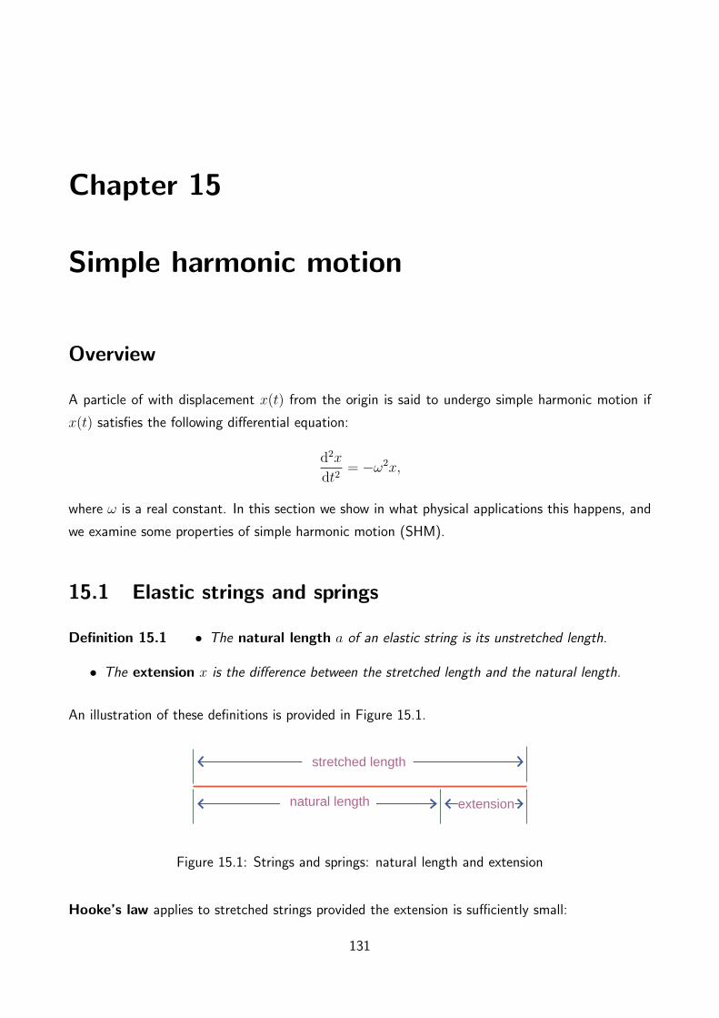
Chapter 15
Simple harmonic motion
Overview
A particle of with displacement x(t) from the origin is said to undergo simple harmonic motion if
x(t) satisfies the following differential equation:
d2x
dt2= −ω2x,
where ω is a real constant. In this section we show in what physical applications this happens, and
we examine some properties of simple harmonic motion (SHM).
15.1 Elastic strings and springs
Definition 15.1 • The natural length a of an elastic string is its unstretched length.
• The extension x is the difference between the stretched length and the natural length.
An illustration of these definitions is provided in Figure 15.1.
extensionnatural length
stretched length
Figure 15.1: Strings and springs: natural length and extension
Hooke’s law applies to stretched strings provided the extension is sufficiently small:
131

132 Chapter 15. Simple harmonic motion
Definition 15.2 Hooke’s law states that the extension in a stretched elastic string is proportional
to the tension T in the string:
T ∝ x or T = kx,
where k is a positive constant.
We usually write k = λ/a, where a is the natural length. Then, Hooke’s law reads
T = λ(x/a) (15.1)
The constant λ = ka is called the modulus of elasticity. Note that λ has the same units as force
– in SI units, Newtons.
15.1.1 Limitation
Hooke’s law holds only up to a point – for sufficiently small extensions. The definition of ‘sufficiently
small’ is a bit circular here – by ‘sufficiently small extension’ we mean those extensions for which
Hooke’s law holds. But this is not facetious: this is a measurable limit called the elastic limit.
Beyond the elastic limit the string will lose its shape once the extension in the string is shrunk back
down to zero. This is hysteresis. The end of this regime corresponds to the plastic limit. Beyond
the plastic limit the string will snap – this corresponds to very large extensions.

15.2. Elastic strings and circular motion!! 133
15.2 Elastic strings and circular motion!!
Example: One end of an elastic string AB is
fixed to a point on a smooth table. A particle
P is attached to the other end and moves in a
horizontal circle with centre A and radius r.
The elastic string AB has natural length 2.5
m and its modulus is 40 N. The mass of P is
5 kg.
If the string is extended by 0.5 m find the speed
of P.
r
P
T
A
B
Solution:
mv2
r= T,
T =λx
`,
mv2
r=λx
`.
v2 =λxr
m`=λx(`+ x)
m`
=40× 0.5× 3
5× 2.5= 4.8.
Hence, v = 2.19 m/s.
Example: If in the above example P has mass 1.5 kg and its speed is 6 m/s and the extension
of the string is 0.4 m find its modulus given that its natural length is 2 m.
Solution:
mv2
r=λx
`,
λ =mv2`
rx=
mv2`
(`+ x)x
=1.5× 36× 2
2.4× 0.4= 112.5 N.

134 Chapter 15. Simple harmonic motion
Example: An elastic string of natural length
` and modulus of elasticity 2mg has one end
fixed to a point A and has a particle P of mass
m attached to the other end B.
P travels in a horizontal circle with angular
speed ω. The elastic limit occurs when tension
T = 3mg.
Find ω when this state is reached.
PO
mg
T
r
l+x
A
B
Solution: First, do a force balance:
• Vertical direction:
T cos θ = mg.
• Horizontal direction – circular motion:
T sin θ = mω2r,
where r is the radius of the circular motion.
But we are given that T = 3mg, hence
ω2 =3g sin θ
r.
We need to eliminate θ and r. From trigonometry,
sin θ =r
`+ x,
hencesin θ
r=
1
`+ x,
hence
ω2 =3g
`+ x=
3g/`
1 + (x/`). (15.2)
We eliminate x/` via Hooke’s law:
T = 3mg = λ(x/`) = 2mg(x/`) =⇒ (x/`) = 32.

15.2. Elastic strings and circular motion!! 135
Substitute into Equation (15.2):
ω2 =3g/`
1 + 32
=6g
5`,
hence
ω =
√6g
5`.
Example: A light elastic string of natural
length 1 m and modulus 35 N is fixed at one
end, and a particle of mass 2 kg is attached to
the other end.
Find the length of the string at equilibrium.
2g
T
x
1m
Solution – we have T = λ(x/a). In equilibrium,
T = mg =⇒ x = mga/λ.
Filling in gives
x = 2× 9.8× 1/35 = 0.56 m,
and hence, the length at equilibrium is
L = x+ a = 1.56 m.
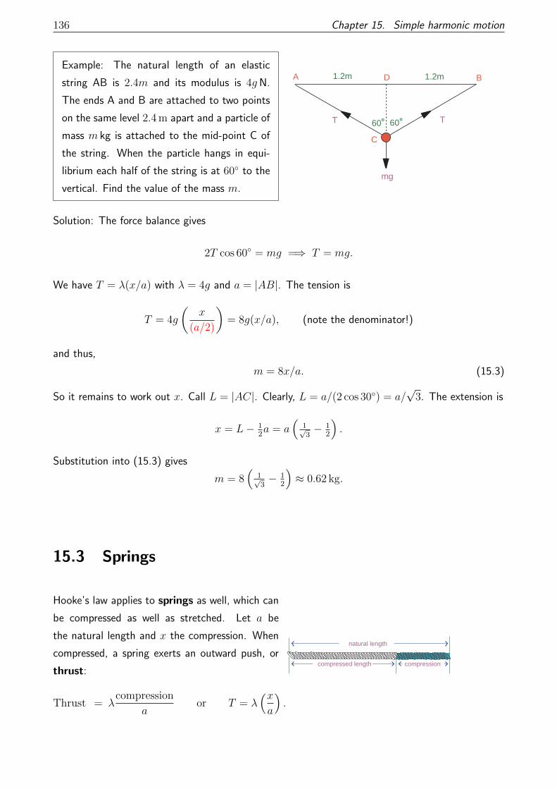
136 Chapter 15. Simple harmonic motion
Example: The natural length of an elastic
string AB is 2.4m and its modulus is 4gN.
The ends A and B are attached to two points
on the same level 2.4 m apart and a particle of
mass m kg is attached to the mid-point C of
the string. When the particle hangs in equi-
librium each half of the string is at 60◦ to the
vertical. Find the value of the mass m.
A
mg
TT
B
C
D 1.2m1.2m
60o60o
Solution: The force balance gives
2T cos 60◦ = mg =⇒ T = mg.
We have T = λ(x/a) with λ = 4g and a = |AB|. The tension is
T = 4g
(x
(a/2)
)= 8g(x/a), (note the denominator!)
and thus,
m = 8x/a. (15.3)
So it remains to work out x. Call L = |AC|. Clearly, L = a/(2 cos 30◦) = a/√
3. The extension is
x = L− 12a = a
(1√3− 1
2
).
Substitution into (15.3) gives
m = 8(
1√3− 1
2
)≈ 0.62 kg.
15.3 Springs
Hooke’s law applies to springs as well, which can
be compressed as well as stretched. Let a be
the natural length and x the compression. When
compressed, a spring exerts an outward push, or
thrust:
Thrust = λcompression
aor T = λ
(xa
).
compressioncompressed length
natural length

15.4. Work done to stretch a spring 137
15.3.1 The sign of the force in Hooke’s law
We take T ≡ F and k = λ/a in Hooke’s Law. Allowing for compression and expansion (i.e. springs),
we have
F = −kx
for the properly-signed string/spring force before the onset of the plastic limit. We have
• For extension, x > 0, hence F < 0, and the spring is accelerated in a negative x-direction,
i.e. back towards x = 0;
• For compression, x < 0, hence F > 0, and the spring is accelerated in a positive x-direction,
i.e. back towards x = 0 again.
For this reason, the force in Hooke’s law is called a restoring force because the force drives any
deviation in x away from zero back towards the equilibrium position at x = 0.
15.4 Work done to stretch a spring
Recall, the work done by a force in moving a particle from x1 to x2 is
W =
∫ x1
x2
F dx.
For Hooke’s Law, F = −kx
W = −∫ x1
x2
kx dx,
= −12k(x2
2 − x21).
Equally from before, the potential function is
U(x) = −∫ x
ref
F (x) dx.
Taking the reference position to be x = 0, this is
U(x) = −∫ x
0
(−kx)dx = 12kx2.
Thus, the principle of conservation of mechanical energy for the string/spring in the absence of
gravity (i.e. string/spring aligned with earth’s surface) is
E = 12mv2 + 1
2kx2 = Const.
138 Chapter 15. Simple harmonic motion
More generally, for the string/spring aligned in the direction of earth’s gravity, we have the following
principle of conservation of mechanical energy:
If a particle of mass m is moving with speed v is at a height h above the zero of
gravitational P.E., and is also attached to an elastic spring stretched by an amount x,
then the mechanical energy is
E =1
2mv2 +mgh+ 1
2kx2.
If no other forces are present, then the above expression for the mechanical energy is a
conserved quantity.

15.4. Work done to stretch a spring 139
15.4.1 Worked examples
Example: One end of a spring, which is strong
enough to stand vertically, is fixed to a point
A on a horizontal plane. A particle of mass
m is attached to the other end of the spring
and is allowed to descend to the equilibrium
position.
Find how much work is done.
l
x
l - x
AA
mg
T
Solution: Displacement:λ
ax = mg, x =
amg
λ.
Work done:
W =λ
2ax2 =
λ
2a
(amgλ
)2
=am2g2
2λ.
Example: A light elastic string (` = 1 m, λ = 7 N) has
one end fixed to a point A. A particle of mass 0.5 kg
hangs in equilibrium at a point C vertically below A.
(a) Find the distance AC.
The particle is raised to B, between A and C where AB
is 1 m and is released from rest.
(b) Find the velocity v at point C.
(c) Find where the particle first comes to rest.
A
B
C
T
12
g
x m
1 m

140 Chapter 15. Simple harmonic motion
Solution – part (a):
T = mg = 12g.
T =λ
`x =
7
1x = 7x.
Therefore
7x = 12g, x = 1
14g = 0.7, |AC| = 1.7 m.
Solution – part (b):
A
B
C v
0.7 m
1 m
0
The reference level is fixed such that, at point B,
Elastic P.E. = 0, Gravitational P.E. = 0.
Also, the K.E. is zero.
At point C, with |BC| = x, the elastic P.E. is
λ
2ax2 =
7
2× 1(0.7)2 = 1.715.
Also, the gravitational P.E. is
−mgx = −0.5× 9.8× 0.7 = −3.41.
The kinetic energy to be determined is
K.E. = 12mv2 = 0.25v2.
By conservation of mechanical energy, the energy at points B and C is the same, hence
0 = 1.715− 3.41 + 0.25v2,
and thus,
v2 = 6.86, v = 2.619 m/s.
Solution – part (c): At the point D, with |BD| = x:
Mechanical Energy =λ
2ax2 −mgx
= 72x2 − 1
2gx = 1
2x(7x− g).
Therefore 12x(7x− g) = 0, hence x = 1
7g = 1.4 m. N.B. x = 0 corresponds to B.

15.4. Work done to stretch a spring 141
Example: A particle P of mass 2m is fas-
tened to the end of each of two identical
elastic strings (equilibrium length ` = 3a,
λ = 3αmg) and is in equilibrium as shown
in the accompanying sketch.
(a) Find α.
(b) Find the mechanical energy of the system.
(c) The particle is now raised to C and re-
leased. Find v at D.
P
2
TT
mg
a4 ACB
DP
a3
a5
a4
a5
Solution – part (a). Tension:
T =λ
3a(5a− 3a) =
2λ
3=
2× 3mgα
3= 2mgα.
Hence,
2T cos θ = 2mg,
4mgα× (3/5) = 2mg,
α = 1012
= 56.
Solution – part (b). Find the mechanical energy of the system:
Elastic P.E. = 2× λ
2× 3a× (2a)2
= 2× 3mgα
6a× 4a2
= 4mgaα =10
3mga
Gravitational P.E. = −3a × 2mg = −6mga. Also, the kinetic energy is zero. Hence, the total
mechanical energy is
Mechanical Energy = 103mga− 6mga = −8
3mga.

142 Chapter 15. Simple harmonic motion
Solution – part (c). Find v at D. We have:
Elastic P.E. at C = 2× λ
2× 3a× a2
= 2× 3mgα
6a× a2
= mgaα
= 56mga
The gravitational potential energy and the kinetic energy are both zero at C, and the mechanical,
so the total mechnical energy is got as follows:
• Elastic P.E. at C – (5/6)mga
• Gravitational P.E. at C – 0
• Kinertic energy at C – 0
for a total mechanical energy (5/6)mga.
Now, the mechnical energy at D is the mechanical energy for a particle at rest (see (b)) plus the
kinetic energy:
Mechnical energy = −83mga+ 1
2(2mv2) = −8
3mga+mv2.
By conservation of mechanical energy,
mechanical energy at C = mechnical energy at D,
hence
−83mga+mv2 = 5
6mga,
mv2 = 83mga+ 5
6mga
= 216mga = 7
2mga.
v2 = 7ga2,
v =
√7ga
2.

15.5. Simple harmonic motion 143
15.5 Simple harmonic motion
For a particle attached to a spring obeying Hooke’s Law, we have F = −kx. But by Newton’s
second law,
F = ma = md2x
dt2,
hence
md2x
dt2= kx.
Dividing across by m and calling
ω =√k/m,
we haved2x
dt2= −ω2x.
This is precisely the equation of simple harmonic motion:
Definition 15.3 A particle of with displacement x(t) from the origin is said to undergo simple
harmonic motion if x(t) satisfies the following differential equation:
d2x
dt2= −ω2x, (15.4)
where ω is a real constant.
The differential equation (15.4) has a definite solution:
Theorem 15.1 The solution to Equation (15.4) can be written as
x(t) = x0 sin(ωt+ φ), (15.5)
where x0 and φ are constants.
Proof: The trial solution (15.5) is plugged into the L.H.S. and the R.H.S. of Equation (15.4) and
agreement between the two sides is sought:
L.H.S =d2x
dt2,
=d2
dt2x0 sin(ωt+ φ),
= −ω2x0 sin(ωt+ φ).
and
R.H.S. = −ω2x = −xω2 sin(ωt+ φ).

144 Chapter 15. Simple harmonic motion
We obtain L.H.S = R.H.S. and thus the trial solution (15.5) is indeed a solution of the differential
equation (15.4). In later modules you will find out that this trial solution is in fact the unique
general solution of Equation (15.4).

15.5. Simple harmonic motion 145
15.5.1 The period
We have
x(t+2π
ω) = x0 sin (ω(t+ (2π/ω)) + φ) ,
= x0 sin ((ωt+ φ) + 2π) ,
= x0 sin(A+ 2π), A = ωt+ φ,
= x0 sin(A),
= x0 sin(ωt+ φ).
Thus, x(t) repeats itself every 2π/ω seconds.
Definition 15.4 The time length T = 2π/ω is called the period of the simple harmonic motion.
Referring to Figure 15.2
x t( )
t
x0
-x0
T
Figure 15.2: Graph of x(t) = x0 sin(ωt+ φ)
for x(t) = x0 sin(ωt+ φ), we have
• T is the time from peak to peak or trough to trough.
• x0 is called the amplitude.
• ω is called the angular frequency.
• ν = 1T
is called the frequency.
• φ is called the phase.
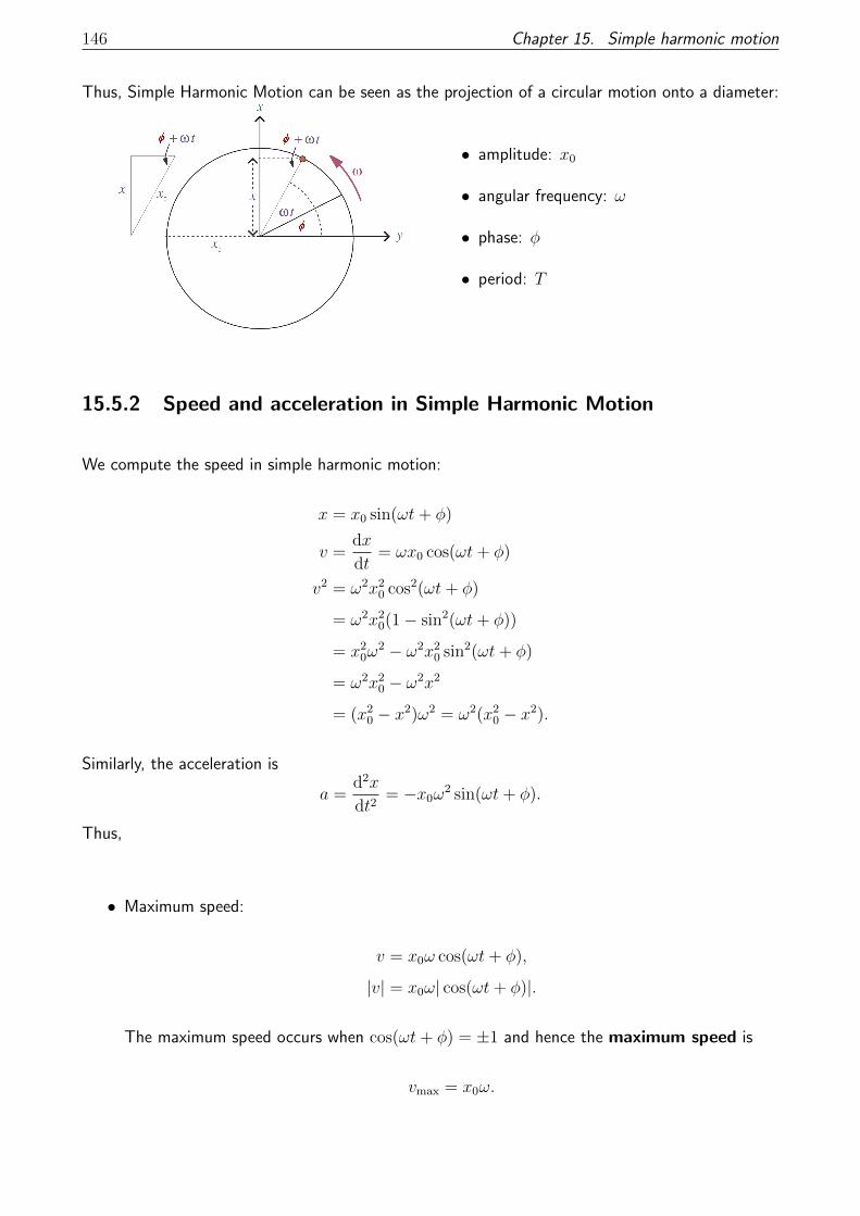
146 Chapter 15. Simple harmonic motion
Thus, Simple Harmonic Motion can be seen as the projection of a circular motion onto a diameter:
• amplitude: x0
• angular frequency: ω
• phase: φ
• period: T
15.5.2 Speed and acceleration in Simple Harmonic Motion
We compute the speed in simple harmonic motion:
x = x0 sin(ωt+ φ)
v =dx
dt= ωx0 cos(ωt+ φ)
v2 = ω2x20 cos2(ωt+ φ)
= ω2x20(1− sin2(ωt+ φ))
= x20ω
2 − ω2x20 sin2(ωt+ φ)
= ω2x20 − ω2x2
= (x20 − x2)ω2 = ω2(x2
0 − x2).
Similarly, the acceleration is
a =d2x
dt2= −x0ω
2 sin(ωt+ φ).
Thus,
• Maximum speed:
v = x0ω cos(ωt+ φ),
|v| = x0ω| cos(ωt+ φ)|.
The maximum speed occurs when cos(ωt+ φ) = ±1 and hence the maximum speed is
vmax = x0ω.

15.5. Simple harmonic motion 147
• Maximum acceleration:
a =d2x
dt2= −x0ω
2 sin(ωt+ φ),
|a| = x0ω2| sin(ωt+ φ)|.
The maximum acceleration occurs when sin(ωt+ φ) = ±1 and thus the maximum acceler-
ation is x0ω2.
15.5.3 Worked examples
Example: A particle P is describing SHM with amplitude 2.5 m. When P is 2 m from the centre
of the path, the speed is 3 m/s.
Find
(a) the period,
(b) the maximum speed,
(c) the maximum acceleration.
Solution: We have
x(t) = x0 sin(ωt+ φ),
v2 = ω2(x20 − x2).
x0 = 2.5 m.
When x = 2 and v = 3,
9 = ω2((2.5)2 − 22) = 2.25ω2.
ω2 =9
2.25= 4, ω = 2 rad/s.
Putting it all together, we have
Part (a) – T = 2πω
= 2π2
= π s.
Part (b) – vmax = x0ω = 2× 2.5 = 5 m/s
Part (c) – amax = x0ω2 = 4× 2.5 = 10 m/s2.

148 Chapter 15. Simple harmonic motion
Example: A, B and C in that order are three points on a straight line and a particle P is moving
on that line with SHM. The velocities of P at A, B and C are 0 m/s, 2 m/s and −1 m/s
respectively.
If AB = 1 m and AC = 4 m, find the amplitude and the period of the motion.
Solution: Refer to Figure 15.3.
A B CO
1m 3m
xo
Figure 15.3:
Note that v2 = ω2(x20 − x2). Therefore v = 0 when x = ±x0. Thus A must be at −x0.
• At A: x = −x0.
• At B: x = −x0 + 1, and
22 = ω2(x2
0 − (−x0 + 1)2)
= ω2(x2
0 − x20 + 2x0 − 1
),
4 = ω2(2x0 − 1
),
ω2 =4
2x0 − 1.
15.5. Simple harmonic motion 149
• At C: x = −x0 + 4, and
(−1)2 = ω2(x2
0 − (−x0 + 4)2)
= ω2(8x0 − 16
),
1 = 8ω2(x0 − 2
),
ω2 =1
8(x0 − 2).
4
2x0 − 1=
1
8(x0 − 2),
32(x0 − 2) = 2x0 − 1,
30x0 = 63,x0 =21
10= 2.1 m.
Putting it all together:
ω2 = 44.2−1
= 43.2
= 54
hence
ω =√
5/4 ≈ 1.118 rad/s,
and
T = 2π/ω ≈ 2π/1.118 ≈ 5.619 s.

150 Chapter 15. Simple harmonic motion
15.6 The simple pendulum
A particle, attached to a light rod, and free to swing in a
plane, is called a simple pendulum.
We analyse the dynamics using two different methods.
mg
lh
15.6.1 Force balance
• Tangential acceleration: `θ
• Tangential force: −mg sin θ
• Newton’s second law:
m`θ = −mg sin θ
hence
θ = −g`
sin θ (15.6)
where we have used the ‘dot’ notation for
derivatives:
θ ≡ dθ
dt, θ ≡ d2θ
dt2.
mg
l
T
l
tangentialacceleration

15.6. The simple pendulum 151
15.6.2 Conservation of mechanical energy
Speed of particle = `θ,
K.E. = 12m`2θ2,
P.E. = −mgh = −mg` cos θ,
E = K.E. + P.E. = 12m`2θ2 −mg` cos θ
The total mechanical energy is conserved:
E = 12m`2θ2 −mg` cos θ = Const.
Differentiating with respect to t:
d
dt
(12m`2θ2 −mg` cos θ
)= 0
12m`2 d
dt(θ2)−mg` d
dt(cos θ) = 0
12m`2 d
dt(θ2)−mg` d
dt(cos θ) = 0
Now
d
dt(θ2) = 2θ
dθ
dt= 2θθ,
d
dt(cos θ) = θ
d(cos θ)
dθ= −θ sin θ.
Therefore
m`2θθ +mg`θ sin θ = 0.
Finally,
θ = −g`
sin θ, (15.7)
in agreement with Equation (15.6).
152 Chapter 15. Simple harmonic motion
15.6.3 Small-amplitude approximation
For small θ, we use the limit
limθ→0
sin θ
θ= 1, θ in radians
to write
sin θ ≈ θ
for small θ. Thus, Equation (15.6) (or equivalently, Equation (15.7)) becomes
d2θ
dt2= −g
`θ. (15.8)
This is just the equation for Simple Harmonic Motion again!!
There is a corresponding approximation for cos θ: since sin θ ≈ θ for θ small, we have
sin θ ≈ θ,
− d
dθcos θ ≈ θ,
− cos θ ≈ Const. + 12θ2,
cos θ Const.− 12θ2.
The constant must be equal to unity because cos(0) = 1, hence
cos θ ≈ 1− 12θ2, θ small.
Using this result, the expression for the energy simplifies to
E = 12m`2θ2 −mg`(1− 1
2θ2).
This can be re-written as
E = 12m`2θ2 + 1
2mg`θ2 + Const.,
where the constant is −mg`. As the energy is only defined up to a constant (set by the arbitrary
reference level of the potential-energy function), an equally good expression for the energy is
E = 12m`2θ2 + 1
2mg`θ2,
which in form is identical to the one already considered for Hooke’s Law and Simple Harmonic
Motion.
Now, the frequency of simple harmonic motion for the simple pendulum can be read off from

15.6. The simple pendulum 153
Equation (15.8): it is
ω2 = g/`.
The period is 2π/ω, hence
T = 2π
√`
g. (15.9)

154 Chapter 15. Simple harmonic motion
15.6.4 Worked examples
Example: The period of a simple pendulum is 3τ . If the period is to be reduced to 2τ , find the
percentage change in length.
Solution: Suppose the period is nτ . Then
nτ = T = 2π
√`
g,
n2τ 2 = 4π2 `
g,
` =n2τ 2g
4π2.
We have
` =n2τ 2g
4π2
Let the length be `3 when the period is 3τ and `2 when the period is 2τ . Then
`3 =9τ 2g
4π2and `2 =
τ 2g
π2.
The relative change in the length is
`3 − `2
`3
=5
9≈ 0.55
Convert into a percentage:
100×(`3 − `2
`3
)= 55% .
15.6. The simple pendulum 155
Example: A simple pendulum is 2 m long and the time it takes to perform 50 oscillations is
measured.
(a) On Earth, the time taken is 142 s. Find g on Earth.
(b) On the Moon, the time taken is 341 s. Find the acceleration due to gravity on the moon.
Solution– Part (a). On Earth:
T =142
50= 2.84 s, T = 2π
√2
g.
2π
√2
g= 2.84,√
g
2=
2π
2.84=
π
1.42.
Thus,
g = 2( π
1.42
)2
= 9.78 m/s2.
Solution– Part (b). On the Moon:
T ′ =341
50= 6.82 s, T ′ = 2π
√2
g′.
2π
√2
g′= 6.82,
√g
2=
2π
6.82=
π
3.41.
Finally,
g = 2( π
3.41
)2
= 1.7 m/s2.

Chapter 16
A more detailed treatment of extended
bodies
Overview
In this section we introduce the concept of the turning effect of a force about a point. This is
relevant when the force does not act through the point in question. We make the idea precise by
introducing the moment of a force.
16.1 Forces in equilibrium – extended bodies
We shall consider only coplanar forces, that is, forces in the same plane. Recall, a particle is in
equilibrium if and only if the resultant force on the particle is zero. A similar conclusion can be
drawn for an extended bodies where all the forces act through a single point (e.g. blocks on planes,
cars on inclines, etc.). For the general case of extended bodies, we need to be a bit more careful.
For an extended body experiencing a system of forces, the body is said to be in equilibrium if and
only if:
• The resultant force is zero
• The forces have no turning effect.
In this chapter we will clarify what ‘no turning effect’ means.
156

16.1. Forces in equilibrium – extended bodies 157
Two forces in equilibrium
The principle of ‘no turning effect’ can be seen in the first
instance for two forces in equilibrium. For example, refer to
the figure on the right. Here, the resultant force is zero,
but the turning effect is not zero. These forces are not in
equilibrium.
Two forces in equilibrium must be equal and opposite and
act along the same straight line.
Three forces in equilibrium
Suppose three forces P ,Q, and R are in equilibrium. The vectors P and Q can be represented by
a single force F .
For R to be in equilibrium with P and Q, it must be equal to −F and act along the same line
as F .
This motivates the following definition:
Definition 16.1 Forces acting through the same point are called concurrent.

158 Chapter 16. A more detailed treatment of extended bodies
We therefore have the following principle:
Three forces in equilibrium must be concurrent and can be represented in magnitude
and direction by the sides of a triangle taken in order.
This triangle is called the Triangle of Forces.
Example: A string of length 1 m is fixed at
one end to a point A on a wall; the other end
is attached to a particle of weight 12 N. The
particle is pulled aside by a horizontal force F
Newtons until it is 0.6 m from the wall. Find
the tension in the string and the value of F .
Solution – The forces must form a triangle. We have
sin θ =0.6
1.0= 0.6,
cos θ =√
1− 0.36 =√
0.64 = 0.8,
tan θ =0.6
0.8=
3
4= 0.75.
Hence,
F = 12 tan θ = 12× 0.75 = 9 N
T =12
0.8= 15 N.

16.1. Forces in equilibrium – extended bodies 159
16.1.1 Lami’s Theorem
We have the following important result:
Theorem 16.1 (Lami) If three forces are in equilibrium they are concurrent, and each force is
proportional to the sine of the angle between the other two forces.
Proof – refer to the figure.
We haveP
sin(180◦ − α)=
Q
sin(180◦ − β)=
R
sin(180◦ − γ).
HenceP
sinα=
Q
sin β=
R
sin γ.
Example: A particle of weight 16 N is attached
to one end of a light string whose other end
is fixed. The particle is pulled aside by a hor-
izontal force until the string is at 30◦ to the
vertical. Find the magnitudes of the horizontal
force and the tension in the string.
Solution – by Lami’s theorem
T
sin 90◦=
P
sin 150◦=
16
sin 120◦.

160 Chapter 16. A more detailed treatment of extended bodies
Hence,
T
1=
P
sin 30◦=
16
sin 60◦,
T
1=
P
2=
16√3/2
,
T =16× 2√
3=
32√3
P =16√3/2× 1
2=
16√3.
16.2 Non-concurrent forces – Moment of a force
We have seen that two forces which are equal and opposite need not be in equilibrium. For them
to be in equilibrium their lines of action must be concurrent. The turning effect of a force about a
point depends on whether or not the force and the point in question are concurrent. This motivates
the definition of the moment of a force:
Definition 16.2 The turning effect of a force about a point is given by the magnitude of the force
× the perpendicular distance of the line of action of the force from the point. The turning effect of
a force is called the moment of the force.
For an illustration of this principle, see the sketch on the
right:
The moment of F about O is |F | × d. (16.1)
In the evaluation of the moment, we include the sense of
turning:
+ → anticlockwise,
− → clockwise.
Note that in the above, we took the moment about a point, but we should consider the point
as an axis perpendicular to the plane of the forces. Note also that the unit of moment is Nm
(Newton-metres).

16.2. Non-concurrent forces – Moment of a force 161
Example: Refer to the figure. The rod AB is free to
rotate about the end A. Find the total moment of the
forces about A.
Solution: Moment is
Total Moment = 4× 1− 7× 4 + 6× 5 + [moment of 8 N force]
We can find moment of the 8 N force by looking at the perpendicular distance between its force
vector and the point A:
The moment is thus
−d× |F = −(10 sin 30◦)× 8 = −40 Nm,
where the minus sign is chosen because this particular moment induces a clockwise motion. Hence,
the total moment is
Total Moment = 4× 1− 7× 4 + 6× 5− 40
= 4− 28 + 30− 40 = −34 Nm.

162 Chapter 16. A more detailed treatment of extended bodies
Example: A DIY fan, unable to loosen a pipe fitting,
slips a piece of scrap pipe (a “cheater”) over her wrench
handle. She then applies her full weight of 900 N to the
end of the cheater by standing on it. The distance from
the centre of the fitting to the point where the weight
acts is 0.8 m and the wrench handle and the cheater
make an angle of 19◦ with the horizontal – as in the
figure on the right. Find the magnitude and direction
of the moment she applies about the centre of the pipe
fitting.
Solution – Referring to Figure 16.1, the perpendicular distance between the point O and the line of
force is
` = 0.8× cos(19◦)
and the moment is
F` = 900× 0.8× cos(19◦) = 680 Nm.
The moment produces a clockwise motion and is therefore negative.
Figure 16.1:

16.2. Non-concurrent forces – Moment of a force 163
16.2.1 Couples
Definition 16.3 Two equal and opposite forces which are not concurrent form a couple.
• Since the resultant is zero what characterizes a couple is its turning effect or moment.
• Two couples with the same moment are equivalent.
• For a couple the moment is independent of the axis:
Referring to the figure, the moment about P is
F × a+ F × (d− a) = Fd,
while the moment about Q is
F × (d− b) + F × b = Fd.
We have the following important principle:
A system of coplanar forces whose resultant is zero and whose moment is non-zero are
said to reduce to a couple.
We will use this principle in the following examples.
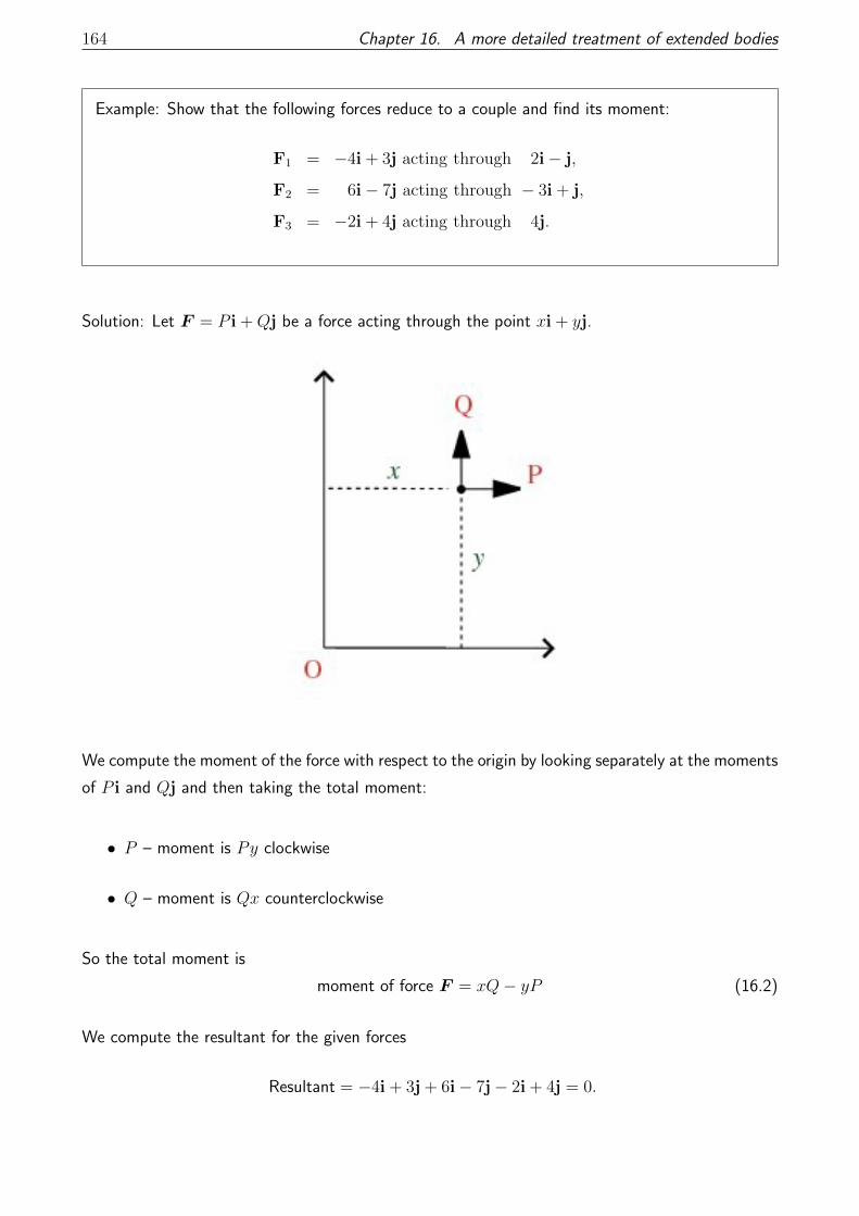
164 Chapter 16. A more detailed treatment of extended bodies
Example: Show that the following forces reduce to a couple and find its moment:
F1 = −4i + 3j acting through 2i− j,
F2 = 6i− 7j acting through − 3i + j,
F3 = −2i + 4j acting through 4j.
Solution: Let F = P i +Qj be a force acting through the point xi + yj.
We compute the moment of the force with respect to the origin by looking separately at the moments
of P i and Qj and then taking the total moment:
• P – moment is Py clockwise
• Q – moment is Qx counterclockwise
So the total moment is
moment of force F = xQ− yP (16.2)
We compute the resultant for the given forces
Resultant = −4i + 3j + 6i− 7j− 2i + 4j = 0.

16.2. Non-concurrent forces – Moment of a force 165
We also compute the total moment, using Equation (16.2) for each force:
Total moment = 2× 3− (−1)(−4)
+(−3)(−7)− 1× 6
+0× 4− 4× (−2)
= 6− 4 + 21− 6 + 8 = 25.
Example: Refer to the figure. ABCD is a
square of side a. Forces of magnitude 1, 2, 3, P
and Q act along−→AB,
−→BC,
−→CD,
−→DA and
−→AC.
Find P and Q if the system reduces to a cou-
ple.
Solution – find the resultant and set it to zero:
Resultant = i− 3i + 2j− P j
+Q cos 45◦i +Q cos 45◦j
= (−2 +Q√
2)i + (2− P +
Q√2
)j.
Hence,
−2 +Q√
2= 0,
2− P +Q√
2= 0.
Finally,
Q = 2√
2,
P =Q√
2+ 2 = 4.
Also, the moment about A is
FBCa+ FCDa = a× 2 + a× 3 = 5a 6= 0.
where FBC denotes the force acting along the length BC etc; the other forces are at a perpendicular
distance of zero from the point A and therefore do not contribute to the total moment.

Chapter 17
Looking Ahead
In later modules, you will find lots of interesting applications of Differential Equations:
• In ACM 10060 (Applications of Differential Equations) you will look at first-order and second-
order differential equations. You will study theory and general methods for finding solutions.
You will study applications in Mechanics, Ecology, and Chaos.
But this is by no means the end of the line. In order to place Mechanics on a proper theoretical
footing, the theory of Differential Equations is crucial. You will continue this study in the following
modules:
• In ACM ACM 20050 (Classical Mechanics and Special Relativity) you will formulate the laws
of planetary motion in differential-equation form – at least for the two-body problem. You will
use techniques from energy conservation and momentum conservation to solve these equations
and thus drive Kepler’s laws of planetary motion from very general first principles.
• In ACM 20060 (Oscillations in Mechanical Systems) you will study mechanical oscillations
using the framework of differential equations. You will look at several interesting applications,
including coupled oscillators and oscillations in the continuum (waves on strings).
• In ACM 30010 (Analytical Mechanics) you will look at how to place the mechanical theories
based on differential equations into a more general theoretical framework called Hamiltonian
mechanics. This framework exposes the very deep mathematical structures that are embedded
in Newton’s laws and paves the way for a theoretical derivation of Quantum Mechanics.
In many of these modules you will be ‘told’ that the solution to
d2x
dt2+ ω2x = 0
166

167
is
x(t) = A sin(ωt+ φ), A, φ = real constants,
or equivalently,
x(t) = w1eiωt + w2e−iωt, w1, w2 = complex constants
but when asked ‘why’ you will most likely (with justification) be told that this is just a clever
trial solution that happens to work. Finally, you in ACM 40690 (Survey of Applied and Compu-
tational Mathematics) you will see the reason why this trial solution works – when the theory of
Laplace Transforms is introduced. Thus, the first and last modules of the ACM degree are linked
through a lengthy and interesting intermediate discussion about Mechanics, Differential Equations,
and advanced topics in Calculus .