University College Dublin An Col aiste Ollscoile, Baile Atha...
195
University College Dublin An Col´ aiste Ollscoile, Baile ´ Atha Cliath School of Mathematics and Statistics Scoil na Matamaitice agus Staitistic´ ı Advanced Fluid Mechanics (ACM 40740) Dr Lennon ´ O N´ araigh Lecture notes in Advanced Fluid Mechanics, January 2016
Transcript of University College Dublin An Col aiste Ollscoile, Baile Atha...

University College Dublin
An Colaiste Ollscoile, Baile Atha Cliath
School of Mathematics and StatisticsScoil na Matamaitice agus Staitisticı
Advanced Fluid Mechanics (ACM 40740)
Dr Lennon O Naraigh
Lecture notes in Advanced Fluid Mechanics, January 2016


Advanced Fluid Mechanics (ACM40740)
• Subject: Applied and Computational Mathematics
• School: Mathematical Sciences
• Module coordinator: Dr Lennon O Naraigh
• Credits: 10
• Level: 4 (Masters)
• Semester: Second
This module introduces advanced concepts and methods in Fluid Dynamics. The main focus is on
viscous incompressible flows, under the following broad headings.
Canonical examples of fluid instability: Eigenvalue analysis of linear instability in the Rayleigh–
Benard, Rayleigh–Taylor, and Kelvin–Helmholtz systems. Eigenvalue analysis of parallel flow insta-
bility leading to the Orr–Sommerfeld equation. Parallel flow instability beyond the temporal
theory: Absolute and convective instability, transient growth Weakly nonlinear stability theory:
Stuart–Landau theory applied to the Cahn–Hilliard and Kuramoto–Sivishinsky equation Turbulence:
Problems in turbulence. Kolmogorov spectra. Wall-bounded turbulence and Reynolds averaging.
Closure models. Discussion of direct numerical simulation and large-eddy simulation. The notion of
wall-functions in large-eddy simulation. Introduction to High-Performance computing: Solving
sparse linear problems iteratively. Applications of such methods to Computational Fluid Dynamics.
Introduction to multithread and multicore programming in Fortran.
What will I learn?
On completion of this module students should be able to
1. Write down the eigenvalue problem for the canonical physical systems of Fluid Dynamics
2. Derive the Orr–Sommerfeld equation and compute exact solutions in certain cases
3. Describe the subtle features of linear stability theory beyond temporal eigenvalue analysis
4. Carry out a Stuart–Landau analysis on simple nonlinear equations
5. Characterize turbulence using the Kolmogorov and Reynolds-averaged theories.
6. Solve sparse linear problems iteratively and implement their solution in Fortran.

In addition to the study of sparse linear systems and their role in Computational Fluid Dynamics,
a number of mini-projects will form part of this module. Therefore, on completion of this module
students should gain much familiarity with computational methods in fluids. In particular, students
should further be able to
1. Perform an Orr–Sommerfeld stability analysis of Poiseuille flow using spectral methods in
Matlab
2. Solve nonlinear wave equations numerically to test for the applicability of Stuart–Landau theory
3. Implement an existing parallel flow solver to study large-eddy simulations in turbulent channel
flow
4. Analyse the turbulent statistics emanating from the simulations under point (4) above.

Editions
First edition: January 2015 This edition: January 2016


Contents
Module description 3
0 Introduction 1
1 Rayleigh–Benard Convection 3
2 Rayleigh–Taylor Instability 22
3 Spectral methods in fluid dynamics 35
4 Stability of viscous parallel flow 47
5 Absolute Instability 65
6 Transient Growth 75
7 Weakly nonlinear theory 95
8 Direct numerical simulation of the incompressible Navier–Stokes equations 104
9 Simplified model problems involving Poisson and Helmholtz equations 115
10 Simplified model problems – numerical setup 125
11 Analysis of numerical setup 130
12 Elements of turbulence theory 139
A M codes 168
7
B Introduction to Fortran 175
Bibliography 184
8
Chapter 0
Introduction
0.1 Overview
The focus of this module is on developing advanced analytical and numerical techniques to deal with
incompressible viscous flow. This is a fairly restricted aim, since many interesting phenomena arise
in treating of the other flow regimes. For example, a study of compressible flow leads to important
topics in acoustics, gas dynamics, and shockwave theory, while a study of incompressible inviscid
flow leads (in two dimensions) to the very beautiful theory of vorticity as described using complex
analysis and conformal-mapping theory. However, it is sensible to maintain a fairly restricted focus,
especially because the proposed research plan aligns with the present lecturer’s expertise. Thus, we
will study the following topics in detail:
• Linear stability analysis for the canonical physical systems of Fluid Dynamics
• Orr–Sommerfeld theory for parallel flow instability, including exact solutions in certain cases
• The subtle features of linear stability theory beyond temporal eigenvalue analysis
• Stuart–Landau analysis for simple nonlinear equations
• Introduction to turbulence using the Kolmogorov and Reynolds-averaged theories.
• Introduction to Computational Fluid Dynamics
0.2 Learning and Assessment
Learning
• One or two lectures per week
1

2 Chapter 0. Introduction
• As this is an advanced module, heavy emphasis is placed on independent study. This will be
guided by lecture notes, recommended textbooks, problem sheets, and computational exer-
cises.
Assessment
• One final exam, counting for 60%1
• Exercises, computational assignments and projects, counting for 40%
Textbooks
Material and exercises for this module will be taken from the following textbooks:
• Hydrodynamic and Hydromagnetic Stability, S. Chandrasekhar (Dover edition, 1981) [Cha61]
• Hydrodynamic Stability, P. G. Drazin, W. H. Reid (Cambridge University Press, 2004 edi-
tion) [DR81]
• Stability and Transition in Shear Flows, P. J. Schmid and D. S. Henningson (Springer,
2001) [SH01]
• Turbulent Flows, S. Pope (Cambridge University Press, 2000) [Pop00]
Other material comes either from the top of my head or from published articles, referred to in the
remainder of the lecture notes.
1The exam will probably run locally in 2014-2015

Chapter 1
Rayleigh–Benard Convection
1.1 Overview
The idea behind the Rayleigh–Benard instability is to take a uniform homogeneous fluid sandwiched
between two plates, and to heat the bottom plate so that a density gradient emerges, with a cooler,
denser layer lying on top of a hotter, less dense layer, thereby inducing an unstable stratification.
Beyond a threshold values, this configuration becomes unstable, triggering a convective motion that
counteracts the unstable stratification. The mathematics of this flow instability is introduced in this
chapter.
1.2 Governing equations
We start with the governing Navier–Stokes equations of incompressible flow in an arbitrary domain:
ρ
(∂ui∂t
+ uj∂ui∂xj
)= − ∂p
∂xi+ µ∇2ui + ρgi,
where all the symbols have their usual meaning and the gravity vector is (g1, g2, g3) = (0, 0,−g),
such that gravity points in the negative z-direction. The Navier–Stokes equation is supplemented
with the incompressibility condition
∂ρ
∂t+
∂
∂xi(ρui) = 0.
To close the Navier–Stokes equations, further conditions (in addition to the incompressibility relation)
are required. In particular, it is necessary to prescribe the behaviour of the density function. In the
present application, we are interested in fluid behaviour in the presence of a temperature gradient,
so it is sensible to focus on a model where the density depends on temperature (T ), wherein the
3

4 Chapter 1. Rayleigh–Benard Convection
simplest possible model is a linear relation:
ρ = ρ0 + δρ, δρ = −ρ0α(T − T0),
where ρ0 is the mean density, δρ is a fluctuation which depends linearly on temperature. Also, T0
is the mean temperature, with T = T0 ⇐⇒ ρ = ρ0. Finally, the quantity α > 0 is the coefficient
of volume expansion. We are not done yet: the evolution of temperature field T (x, t) must be
precribed. However, this can be accurately modelled by an advection-diffusion equation:
∂T
∂t+ ui
∂T
∂xi= κ∇2T,
where κ > 0 is the thermal diffusivity. We assemble all our equations into a single mathematical
model:
ρ
(∂ui∂t
+ uj∂ui∂xj
)= − ∂p
∂xi+ µ∇2ui + ρgi, (1.1a)
∂ρ
∂t+
∂
∂xi(ρui) = 0, (1.1b)
ρ = ρ0 + δρ, δρ = −ρ0α(T − T0), (1.1c)
∂T
∂t+ ui
∂T
∂xi= κ∇2T, (1.1d)
In practice, the density variations are quite small, and an approximation can be made wherein density
variations are considered only in the buoyancy (gravity) term. This is called the Boussinesq
Approximation (for a full justification of this approximation, see pages 16-17 in [Cha61]. Thus,
Equations (1.1a)–(1.1b) simplify to
∂ui∂t
+ uj∂ui∂xj
= − 1
ρ0
∂p
∂xi+ ν∇2ui +
(1 +
δρ
ρ0
gi
), ν = µ/ρ0, (1.2a)
∂ui∂xi
= 0, (1.2b)
while the density and temperature laws remain unchanged. This is a great simplification, as the
density in the Navier–Stokes equations is now ‘almost’ a constant.
1.3 The base state
We study a time-independent base state involving no flow, with ui = 0 and a static temperature
distribution, such that
∇2T = 0.
1.3. The base state 5
We also focus on a two-dimensional geometry for now, in the (x, z) plane, such that the solution of
the Laplace equation for temperature reads
T = T0 + Ax+Bz,
where A and B are constants. However, we specialize without loss of generality to a situation where
the temperature gradient is imposed in the z-direction only, such that A = 0. Also, we focus on
the more interesting case of an adverse temperature gradient, such that B = −β, with β > 0, and
such that
T = T0 − βz.
Thus, compared to a baseline at z = 0 where the temperature is T0, high up where z > 0 it is
relatively colder and low down where z < 0 it is relatively hotter. Next, using ρ = ρ0 + δρ =
ρ0 − αρ0(T − T0) we obtain
ρ = ρ0(1 + αβz).
Again, compared to a baseline at z = 0 where the density is ρ0, high up where z > 0 the fluid is
both relatively cool and relatively more dense while low down where z < 0 it is relatively hot and
less dense. This is the notion of an adverse temperature gradient - the temperature and density
gradients are going in opposite directions. The last part of the characterization of the base state is
the determination of the pressure. We have the w-velocity equation:
∂w
∂t+ u
∂w
∂x+ w
∂w
∂z= −∂p
∂z− ρ0g(1 + αβz) + ν∇2w.
With w = 0 this gives∂p
∂z= −ρ0g(1 + αβz). (1.3)
The analogous u-velocity equation gives ∂p/∂x = 0. Note that Equation (1.3) is the equation of
hydrostatic balance: the pressure drop and the gravity force are balanced. Solving Equation (1.3)
gives
p = −ρ0g(z + 1
2αβz2
).
We now characterize the base state in full by assembling our results in one place:
ui = 0, p = −ρ0g(z + 1
2αβz2
). (1.4a)
T = T0 − βz, ρ = ρ0(1 + αβz). (1.4b)

6 Chapter 1. Rayleigh–Benard Convection
1.4 Linear stability analysis
Equations (1.4) are the time-independent base state of the problem. This solution would appear
to be unstable as the stratification is (apparently) itself unstable: a denser fluid sits on top of a less
dense fluid. The idea of the remainder of this chapter is to investigate this stability problem. We
do so by introducing perturbations:
ui = 0︸︷︷︸base state
+ ui︸︷︷︸perturbations
and
T ′ = T0 − βz︸ ︷︷ ︸base state
+ θ︸︷︷︸perturbations
.
We assume that the perturbations are small in the sense that the equations of motion for (ui, T′)
can be linearized without any loss of accuracy in the modeling. The linearized equations of motion
read
∂ui∂t
= − ∂
∂xi
(δp
ρ0
)− δi,zgαθ + ν∇2ui, (1.5a)
∂ui∂xi
= 0, (1.5b)
∂θ
∂t= wβ + κ∇2θ. (1.5c)
Here, δp is the perturbation pressure.
Exercise 1.1 Prove Equation (1.5) by carrying out the relevant linearization.
In incompressible flow wherein the density is a fixed constant, the pressure is always a ‘bad’ variable
because it does not have its own equation (it is determined implicitly via the relation ∂iui = 0).
Thus, we always try to eliminate the pressure from the equations of motion. We do that here by
considering again the momentum equations:
∂u
∂t= − ∂
∂x
(δp
ρ0
)+ ν∇2u, (1.6)
∂w
∂t= − ∂
∂z
(δp
ρ0
)− gαθ + ν∇2w, (1.7)
1.4. Linear stability analysis 7
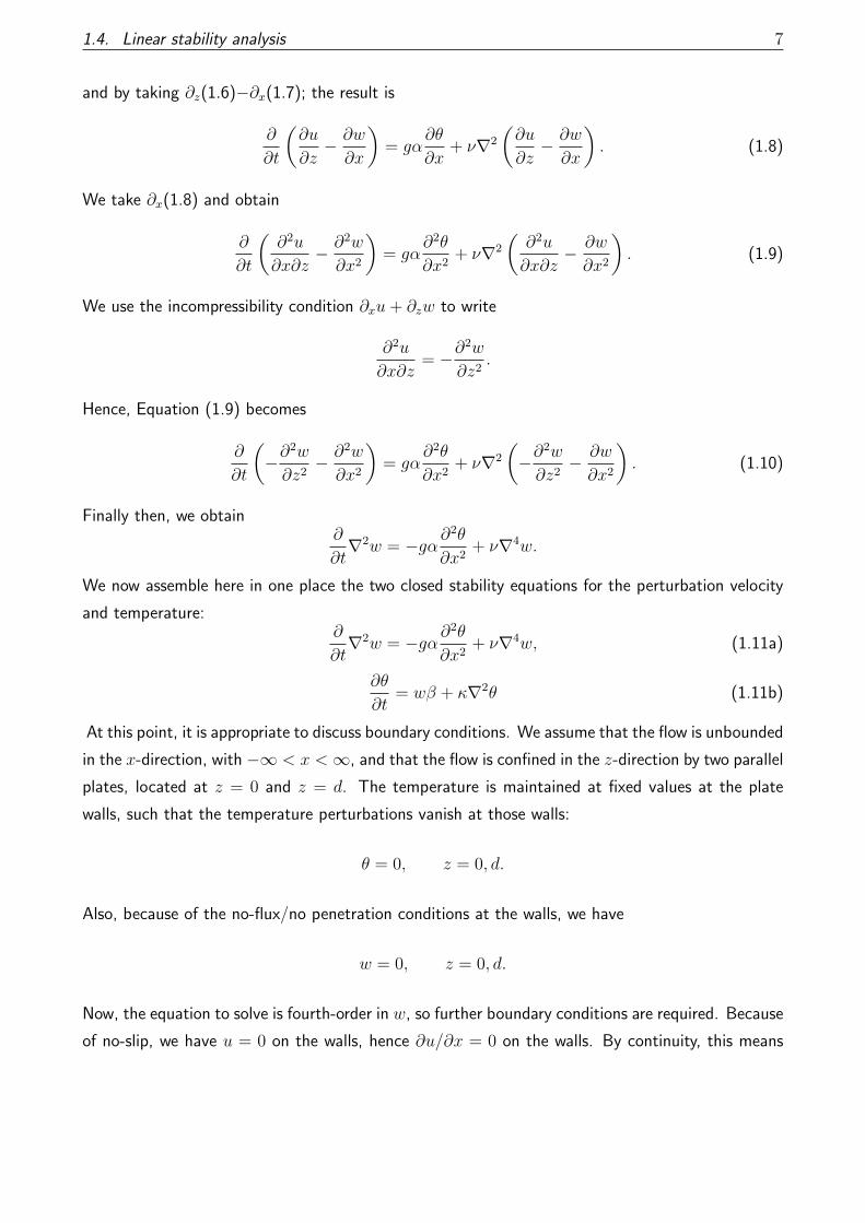
and by taking ∂z(1.6)−∂x(1.7); the result is
∂
∂t
(∂u
∂z− ∂w
∂x
)= gα
∂θ
∂x+ ν∇2
(∂u
∂z− ∂w
∂x
). (1.8)
We take ∂x(1.8) and obtain
∂
∂t
(∂2u
∂x∂z− ∂2w
∂x2
)= gα
∂2θ
∂x2+ ν∇2
(∂2u
∂x∂z− ∂w
∂x2
). (1.9)
We use the incompressibility condition ∂xu+ ∂zw to write
∂2u
∂x∂z= −∂
2w
∂z2.
Hence, Equation (1.9) becomes
∂
∂t
(−∂
2w
∂z2− ∂2w
∂x2
)= gα
∂2θ
∂x2+ ν∇2
(−∂
2w
∂z2− ∂w
∂x2
). (1.10)
Finally then, we obtain∂
∂t∇2w = −gα∂
2θ
∂x2+ ν∇4w.
We now assemble here in one place the two closed stability equations for the perturbation velocity
and temperature:∂
∂t∇2w = −gα∂
2θ
∂x2+ ν∇4w, (1.11a)
∂θ
∂t= wβ + κ∇2θ (1.11b)
At this point, it is appropriate to discuss boundary conditions. We assume that the flow is unbounded
in the x-direction, with −∞ < x <∞, and that the flow is confined in the z-direction by two parallel
plates, located at z = 0 and z = d. The temperature is maintained at fixed values at the plate
walls, such that the temperature perturbations vanish at those walls:
θ = 0, z = 0, d.
Also, because of the no-flux/no penetration conditions at the walls, we have
w = 0, z = 0, d.
Now, the equation to solve is fourth-order in w, so further boundary conditions are required. Because
of no-slip, we have u = 0 on the walls, hence ∂u/∂x = 0 on the walls. By continuity, this means
8 Chapter 1. Rayleigh–Benard Convection
that∂w
∂z= 0, z = 0, d,
and this gives the required number of boundary conditions necessary to solve Equations (1.11).
1.5 Normal-mode solution
Because of the translational invariance of the equations (1.11) in the x-direction, it makes sense
to introduce a trial solution w ∝ eikx and θ ∝ eikx representing a plane wave, where k is the
wavenumber. Indeed, it also makes sense to introduce exponential time dependence (in a standard
way) such that the following normal-mode solution is proposed:
w = ept+ikxW (z), (1.12a)
θ = ept+ikxΘ(z). (1.12b)
Substitution of Equations (1.12) into Equations (1.11) yields
p(∂2z − k2
)W = ν
(∂2z − k2
)2W − gαk2Θ,
pΘ = βW + κ(∂2z − k2
)Θ.
Before going any further, we reduce the number of parameters in these equations by rescaling as
follows: (∂2z − k2 − p
κ
)Θ = −β
κW, (1.13a)(
∂2z − k2
) (∂2z − k2 − p
ν
)W =
gα
νk2Θ. (1.13b)
We introduce a non-dimensional z-coordinate z = z/d, with
d
dz=dz
dz
d
dz=
1
d
d
dz,
and the equations (1.13) become(∂2z − d2k2 − pd2
ν
ν
κ
)Θ = −βd
2
κW, (1.14a)
(∂2z − d2k2
)(∂2z − d2k2 − pd2
ν
)W =
gαd2
ν(d2k2)Θ. (1.14b)
We identify
Pr =ν
κ, σ =
pd2
ν, [σ] = 1,

1.5. Normal-mode solution 9
where Pr = ν/κ is the Prandtl number. Thus, Equations (1.14) become
(∂2z − k2 − σPr
)Θ = −βd
2
κW, (1.15a)(
∂2z − k2
)(∂2z − k2 − σ
)W =
gαd2
νk2Θ, (1.15b)
where k = dk is a dimensionless wavenumber . We combine the Θ and W -equations by taking the
W -equation and operating on it with (∂ − z2 − k2 − σ Pr). We obtain
(∂2z − k2 − σPr
) [(∂2z − k2
)(∂2z − k2 − σ
)W]
=(∂2z − k2 − σPr
)[gαd2
νk2Θ
],
=gαd2
νk2[(∂2z − k2 − σPr
)Θ],
=gαd2
νk2
[−βd
2
κW
],
= −gαβd4
νκk2W.
We introduce
Ra =gαβd4
νκ
as the Rayleigh number and we have the following single stability equation:(∂2z − k2 − σPr
)(∂2z − k2 − σ
)(∂2z − k2
)W = −Ra k2W. (1.16a)
Exercise 1.2 Show that the Rayleigh number is dimensionless.
Viewing the eigenvalue problem as an equation in the single variable W , it can be noted that the
ordinary differential equation to solve is sixth order. We already have the boundary conditions
W = W ′ = 0, z = 0, 1, (1.16b)
giving four boundary conditions. We need two more boundary conditions to close the problem.
However, since (∂2z − k2)(∂2
z − k2 − σ)W = (gαd2/ν)k2Θ, and since Θ = 0 on the boundaries, the
remaining two boundary conditions are given by(∂2z − k2 − σ
)(∂2z − k2
)W = 0, z = 0, 1. (1.16c)
10 Chapter 1. Rayleigh–Benard Convection
Thus, we have an ordinary differential equation in the eigenvalue σ. Before attempting various
approaches to solve for σ as a function of k explicitly, we first of all investigate the properties of
this equation using a priori methods. Following standard practice, in the remainder of this Chapter
we omit the tildes over the dimensionless variables.
1.6 A priori methods for the stability equation
We prove the following theorem:
Theorem 1.1 Consider the eigenvalue problem given by Equation (1.16). The eigenvalue σ is
purely real and therefore, the transition from stability to instability is given by σ = 0.
Proof: Introduce
G = (∂2z − k2)W, F = (∂2
z − k2)(∂2z − k2 − σ)W,
hence F = (∂2z −k2−σ)G. The boundary conditions in Equation (1.16) imply that F = 0 at z = 0
and z = 1. Also, the eigenvalue equation can be rewritten as
(∂2z − k2 − Prσ)F = −Ra k2W.
We multiply both sides of this equation by F ∗ and integrate from z = 0 to z = 1. Now,∫ 1
0
F ∗∂2zF dz = −
∫ 1
0
|∂zF |2 dz,
in view of the boundary conditions on F at z = 0 and z = 1. Thus, we obtain∫ 1
0
[|∂zF |2 + (k2 + Prσ)|F |2
]dz = Ra
∫ 1
0
F ∗W dz.
Now consider ∫ 1
0
F ∗W dz =
∫ 1
0
W (∂2z − k2 − σ∗)G∗ dz,
=
∫ 1
0
W∂2zG∗ dz − (k2 + σ∗)
∫ 1
0
WG∗ dz,
=
∫ 1
0
G∗∂2zW dz − (k2 + σ∗)
∫ 1
0
WG∗ dz,
=
∫ 1
0
G∗[(∂2z − k2)− σ∗
]W dz,

1.6. A priori methods for the stability equation 11
where we have used integration by parts repeatedly to show that∫ 1
0
W∂2zG∗ dz =
∫ 1
0
G∗∂zW dz,
using further the fact that W = ∂zW = 0 on z = 0, 1. Now,∫ 1
0
F ∗W dz =
∫ 1
0
G∗[(∂2z − k2)− σ∗
]W dz,
=
∫ 1
0
G∗ (G− σ∗) dz,
=
∫ 1
0
|G|2 dz − σ∗∫ 1
0
G∗W,
= ‖G‖22 − σ∗
∫ 1
0
[(∂2z − k2
)W ∗]W dz,
= ‖G‖22 + σ∗
∫ 1
0
(|∂zW |2 + k2|W |2
)dz
Putting it all together, we have
‖∂zF‖22 + (k2 + Prσ)‖F‖2
2 = Ra[‖G‖2
2 + σ∗(‖∂zW‖2
2 + k2‖W‖22
)]Take imaginary parts on both sides of this equation:
Pr=(σ)‖F‖22 = −Ra=(σ)
(‖∂zW‖2
2 + k2‖W‖22
),
where the mysterious minus sign emerges on the right-hand side because it is σ∗ that appears there,
not σ. Hence,
=(σ)[Pr‖F‖2
2 + Ra(‖∂zW‖2
2 + k2‖W‖22
)]= 0.
Now, the quantity inside the square brackets is positive definite, so we are forced to conclude that
=(σ) = 0.
For the second part of the theorem, we start with the fact that the system changes from stable to
unstable when
<(σ) = 0.
However, σ is purely real, so this condition for a change in the stability amounts to
σ = 0.
This concludes the proof.

12 Chapter 1. Rayleigh–Benard Convection
In stability theory it is of interest to construct the neutral curve <(σ) = 0 as a function of the
problem parameters (in this case (Ra,Pr, k)). For the Rayleigh–Benard convection, we have shown
that the neutral curve amounts to σ(Ra,Pr, k) = 0. In the next section we find semi-explicit
solutions for this neutral curve.
1.7 Explicit solution for the neutral curve
From the previous section, it is known that the neutral curve occurs when σ = 0. Therefore, we set
σ = 0 in the eigenvalue problem (1.16) to obtain the following simplified equations:
(∂2z − k2
)3W = −Ra k2W.
Instead of placing the plates at z = 0, 1, we instead set up the problem in a more symmetric manner,
such that z ∈ (−1/2, 1/2). Thus, the relevant boundary conditions are imposed as follows:
W = W ′ = (∂2z − k2)2W = 0 on z = ±1
2.
We immediately make a trial solution
W = e±qz
such that
(q2 − k2)3 = −Ra k2.
We call
Ra k2 = τ 3k6
hence
(q2 − k2)3 = −τ 3k6,
and
q2 = k2 + (−1)1/3τk2.
Note also:
τ = (Ra/k4)1/3.
The three cube roots of unity are
(−1)1/3 = −1, 12
(1± i√
3),
hence
q2 = −k2(τ − 1), q2 = k2[1 + τ 1
2
(1± i√
3)].
1.7. Explicit solution for the neutral curve 13
Taking square roots, we obtain the following six square-root solutions:
±iq0, ±q, ±q∗,
where q0 = k√τ − 1 and
<(q) := q1 = k[
12
√1 + τ + τ 2 + 1
2
(1 + 1
2τ)]1/2
, (1.17a)
=(q) := q2 = k[
12
√1 + τ + τ 2 − 1
2
(1 + 1
2τ)]1/2
. (1.17b)
Exercise 1.3 Prove Equation (1.17).
In view of the symmetric nature of the problem (sandwiched between z = −1/2 and z = 1/2), we
can break up the solution into odd and even cases with respect to the centreline at z = 0. For the
even case we have a solution
W = A0 cos(q0z) + A cosh(qz) + A∗ cosh(q∗z),
where we have constructed a manifestly even solution via a linear superposition of component
solutions. There are only three linearly independent complex coefficients in the superposition, and
these can be chosen as A0, A, and A∗, since A and A∗ are linearly independent. Imposing the
boundary conditions at z = ±1/2 yields
A0 cos(q0/2) + A cosh(q/2) + A∗ cosh(q∗/2) = 0, (1.18a)
−q0A0 sin(q0/2) + qA sinh(q/2) + q∗A∗ sinh(q∗/2) = 0, (1.18b)
A0 cos(q0/2) + 12
(i√
3− 1)A cosh(q/2)− 1
2
(i√
3 + 1)A∗ cosh(q∗/2) = 0. (1.18c)
This immediately leads to a determinant problem∣∣∣∣∣∣∣∣cos(q0/2) cosh(q/2) cosh(q∗/2)
−q0 sin(q0/2) q sinh(q/2) q∗ sinh(q∗/2)
cos(q0/2) 12
(i√
3− 1)
cosh(q/2) −12
(i√
3 + 1)
cosh(q∗/2)
∣∣∣∣∣∣∣∣ = 0. (1.19)
14 Chapter 1. Rayleigh–Benard Convection
We divide each row of the determinant problem by the first row to obtain∣∣∣∣∣∣∣∣1 1 1
−q0 tan(q0/2) q tanh(q/2) q∗ tanh(q∗/2)
1 12
(i√
3− 1)−1
2
(i√
3 + 1)∣∣∣∣∣∣∣∣ = 0. (1.20)
Next, we subtract the first row from the third row and divide the result by −√
3/2 to obtain∣∣∣∣∣∣∣∣1 1 1
−q0 tan(q0/2) q tanh(q/2) q∗ tanh(q∗/2)
0√
3− i√
3 + i
∣∣∣∣∣∣∣∣ = 0. (1.21)
Expanding this determinant yields
=[(√
3 + i)q tanh(q/2)
]+ q0 tan(q0/2) = 0. (1.22)
Exercise 1.4 Fill in the blanks in the derivations of Equations (1.18), (1.21) and (1.22).
Since q and q0 are both functions of k and Ra, Equation (1.22) can be regarded as a condition of
the form
Φ(Ra, k) = 0,
where Φ is a function of two variables. This is the implicit equation of a curve in Ra − k space
– the neutral curve. Note that the neutral curve is independent of the Prandtl number. Thus, to
determine the onset of instability, the Prandtl number is irrelenvant - only the wavenumber and the
Rayleigh number matter. The aim of the remainder of this section is to compute the neutral curve
numerically.
1.7. Explicit solution for the neutral curve 15
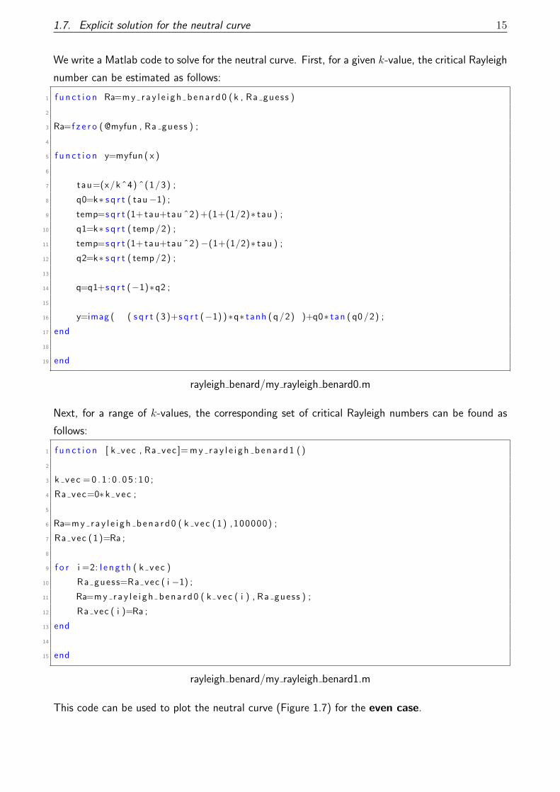
We write a Matlab code to solve for the neutral curve. First, for a given k-value, the critical Rayleigh
number can be estimated as follows:
1 f u n c t i o n Ra=m y r a y l e i g h b e n a r d 0 ( k , R a g u e s s )
2
3 Ra=f z e r o ( @myfun , R a g u e s s ) ;
4
5 f u n c t i o n y=myfun ( x )
6
7 tau =(x/k ˆ4) ˆ(1/3) ;
8 q0=k∗ s q r t ( tau−1) ;
9 temp=s q r t (1+ tau+tau ˆ2) +(1+(1/2)∗ tau ) ;
10 q1=k∗ s q r t ( temp /2) ;
11 temp=s q r t (1+ tau+tau ˆ2)−(1+(1/2)∗ tau ) ;
12 q2=k∗ s q r t ( temp /2) ;
13
14 q=q1+s q r t (−1)∗q2 ;
15
16 y=imag ( ( s q r t ( 3 )+s q r t (−1) ) ∗q∗ tanh ( q /2) )+q0∗ tan ( q0 /2) ;
17 end
18
19 end
rayleigh benard/my rayleigh benard0.m
Next, for a range of k-values, the corresponding set of critical Rayleigh numbers can be found as
follows:
1 f u n c t i o n [ k vec , Ra vec ]= m y r a y l e i g h b e n a r d 1 ( )
2
3 k v e c = 0 . 1 : 0 . 0 5 : 1 0 ;
4 Ra vec=0∗k v e c ;
5
6 Ra=m y r a y l e i g h b e n a r d 0 ( k v e c ( 1 ) ,100000) ;
7 Ra vec ( 1 )=Ra ;
8
9 f o r i =2: l e n g t h ( k v e c )
10 R a g u e s s=Ra vec ( i −1) ;
11 Ra=m y r a y l e i g h b e n a r d 0 ( k v e c ( i ) , R a g u e s s ) ;
12 Ra vec ( i )=Ra ;
13 end
14
15 end
rayleigh benard/my rayleigh benard1.m
This code can be used to plot the neutral curve (Figure 1.7) for the even case.
16 Chapter 1. Rayleigh–Benard Convection
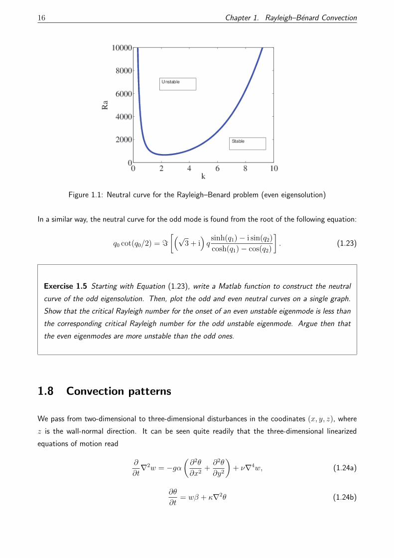
Figure 1.1: Neutral curve for the Rayleigh–Benard problem (even eigensolution)
In a similar way, the neutral curve for the odd mode is found from the root of the following equation:
q0 cot(q0/2) = =[(√
3 + i)q
sinh(q1)− i sin(q2)
cosh(q1)− cos(q2)
]. (1.23)
Exercise 1.5 Starting with Equation (1.23), write a Matlab function to construct the neutral
curve of the odd eigensolution. Then, plot the odd and even neutral curves on a single graph.
Show that the critical Rayleigh number for the onset of an even unstable eigenmode is less than
the corresponding critical Rayleigh number for the odd unstable eigenmode. Argue then that
the even eigenmodes are more unstable than the odd ones.
1.8 Convection patterns
We pass from two-dimensional to three-dimensional disturbances in the coodinates (x, y, z), where
z is the wall-normal direction. It can be seen quite readily that the three-dimensional linearized
equations of motion read
∂
∂t∇2w = −gα
(∂2θ
∂x2+∂2θ
∂y2
)+ ν∇4w, (1.24a)
∂θ
∂t= wβ + κ∇2θ (1.24b)

1.8. Convection patterns 17
where the differential operators are now in the appropriate three-dimensional form. Under a normal-
mode decomposition
w = ei(kxx+kyy)+ptW (z), θ = ei(kxx+kyy)+ptΘ(z),
the eigenvalue equation derived previously still persists, only now the quantity k2 in the relevant
differential equation means k2 = k2x + k2
y. Thus, there was no loss of generality in our previous
focus on the two-dimensional case. Interestingly, the theory at this stage is by no means complete,
since at the onset of criticality (i.e. for parameters along the neutral curve) there are many ways in
which the critical wavenumber k2c can be resolved into its x- and y-components. Thus, the theory
so far does not tell us which pair (kx, ky) (with k2x+k2
y = k2c ) is selected. Indeed, any pair consistent
with this condition is possible and hence, a linear superposition of all such consistent pairs is the
general acceptable solution.
However, we can observe that a particular wavenumber choice corresponds to a periodic cell, repli-
cated throughout the xy-plane. Because the problem is translationally invariant in the xy-plane,
these cells should fill in the xy plane with no gaps. There is a loose analogy here with solid-state
physics: translational symmetry in a discrete crystal structure implies a lattice structure, which in
turn implies that the only possibility for the unit cell (in two dimensions) is a square, an equilateral
triangle, or a hexagon. Thus, only those wavenumber combinations that produce a square,
equilateral triangle or a hexagon as the periodic cell are allowed by the translational
symmetry of the problem. This completes the theory.
The complete velocity field
The complete velocity field (u, v, w) can be backed out from these considerations, albeit in a re-
markably roundabout fashion. First, we note that
w = F (x, y)W (z),
where F (x, y) is that combination of complex exponentials that gives the relevant periodic unit cell,
such that (∂
∂x,∂
∂y, 0
)F = −k2F.
Because of its ubiquity in the following, we call
∇⊥ =
(∂
∂x,∂
∂y, 0
),
18 Chapter 1. Rayleigh–Benard Convection
hence ∇2⊥F = −k2F . Next, we introduce the wall-normal component of the vorticity,
ζ = z · ω = ∂xv − ∂yu.
We have
∂ζ
∂x=
∂2v
∂x2− ∂2u
∂x∂y, (1.25a)
∂ζ
∂y=
∂2v
∂x∂y− ∂2u
∂y2. (1.25b)
In view of the incompressibility condition ∂xu+ ∂yv + ∂zw = 0, we also have
∂2u
∂x∂y= −∂
2v
∂y2− ∂2w
∂y∂z, (1.26a)
∂2v
∂x∂y= −∂
2u
∂x2− ∂2w
∂x∂z. (1.26b)
We combine Equations (1.25)–(1.26) now to obtain
∂ζ
∂x=∂2v
∂x2+∂2v
∂y2+
∂2w
∂y∂z= ∇2
⊥v +∂2w
∂y∂z= −k2v +
∂2w
∂y∂z,
hence
v =1
k2
(∂2w
∂y∂z− ∂ζ
∂x
).
Also,∂ζ
∂y= −∂
2u
∂x2− ∂2w
∂x∂z− ∂2u
∂y2= −∇2
⊥u−∂2w
∂y∂z= k2u− ∂2w
∂y∂z,
hence
u =1
k2
(∂2w
∂x∂z− ∂ζ
∂y
).
However, quite generally, we have the vortex stretching equation, which reads
∂ω
∂t+ u · ∇ω = ω · ∇u+ ν∇2ω,
the linearization of which is∂ω
∂t= ν∇2ω,
and projecting on to the z-direction gives
∂ζ
∂t= ν∇2ζ.

1.8. Convection patterns 19
In normal-mode form, this gives
σζ = (∂2z − k2)ζ.
However, we are at criticality, with σ = 0, hence
(∂2z − k2)ζ = 0, ζ = 0 on z = ±1/2,
the only solution of which is ζ = 0. Hence, the wall-normal component of the vorticity vanishes in
this very particular case, and we are left with
u =1
k2
∂2w
∂y∂z, v =
1
k2
∂2w
∂x∂z.
Letting u⊥ = (u, v), we have
u⊥ =1
k2
∂
∂z
(∂w
∂x,∂w
∂y
)=
1
k2W ′∇⊥F.
But w = F (x, y)W (z), hence F = w/W , hence
u⊥ =1
k2
W ′
W∇⊥w.
Thus, if the gradient ∇⊥w vanishes, then so does u⊥. We now use these results to investigate the
convection cells. We examine only two-dimensional rolls in depth here: the interested reader can
study Chandrasekhar’s book for an in-depth treatment of the three-dimensional structures: rect-
angular, triangular and hexagonal cells. Typical two-dimensional and three-dimensional convection
cells are compared side-by side in Figure 1.2.
Convection rolls
The simplest convection pattern is the roll, wherein ky = 0, and the problem reverts to a two-
dimensional one. Let the critical wavenumber be k. Then , the size of the convection cell is
L = 2π/k. The velocity profile is
w = W (z) cos(kx), k = 2π/L
where W (z) is the eigenfunction corresponding to the eigenvalue σ = 0. The corresponding com-
ponents of the velocity parallel to the wall are
u = −1
kW ′ sin(kx), v = 0.

20 Chapter 1. Rayleigh–Benard Convection
Figure 1.2: Typical two-dimensional and three-dimensional convection cells are compared side-byside. Schematic from Scholarpedia article on Rayleigh–Benard convection (accessed 07/01/2015).
It is clear that an appropriate streamfunction for the flow is
ψ = −1
kW sin(kx),
with u = ∂zψ and w = −∂xψ. The streamlines can be plotted as isosurfaces of the streamfunc-
tion. For the W -component of the streamfunction, I use the approximation W ≈ z2 − 2z3 + z4,
which satisfies the symmetry condition (even function) and boundary conditions but is otherwise an
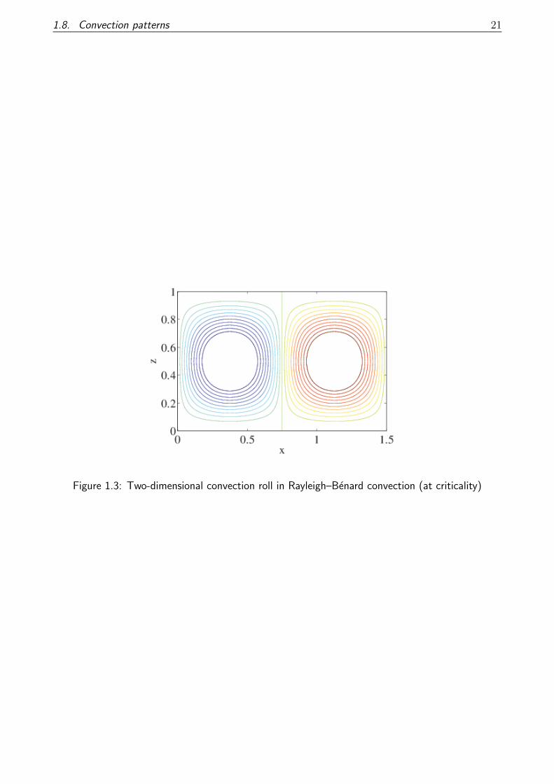
approximation of the true eigenfunction. The result of the plot is shown in Figure 1.3. The main
feature here is two counter-rotating vortices in the cell that act to redistribute the temperature.
This is the essential signature of Rayleigh–Benard convection.
1.8. Convection patterns 21
Figure 1.3: Two-dimensional convection roll in Rayleigh–Benard convection (at criticality)

Chapter 2
Rayleigh–Taylor Instability
2.1 Overview
The idea behind the Rayleigh–Taylor instability is to take two distinct incompressible fluids separated
by a flat interface, such that the heavier fluid sits on top of the lighter one. This is obviously an
unstable situation: we introduce the theory that proves this. This is an important example not only
for the practical applications (some of which are nefarious) but because it is the simplest possible
example of a two-phase flow instability, the stability theory for which admits exact analytical
solutions. In this chapter we will give an account not only of the inviscid theory (wherein those
analytical solutions apply), but the viscous case also. The viscous case gives a nice introduction to
numerical spectral methods for the solution of eigenvalue problems in two-phase flows.
2.2 Stability analysis – Inviscid case
A schematic description of the physical problem is shown in Figure 2.1. The fluid domain is (x, y) ∈R2, and the base-state location of the interface is at z = 0. The density profile is
ρ(x, y) =
ρL, z > 0,
ρG, z < 0,
where ρG and ρL are both constant and ρG < ρL. Thus, it is as though the domain is taken up by
two distinct fluids (or phases). Both phases are however assumed for the time being to be invsicid,
with µi = 0 and i = L,G. The base-state corresponds to a situation with no flow, such that ui = 0,
again with i = L,G.
Interestingly, the equilibrium pressure field P0 is non-trivial. The z-momentum equation in the base
22
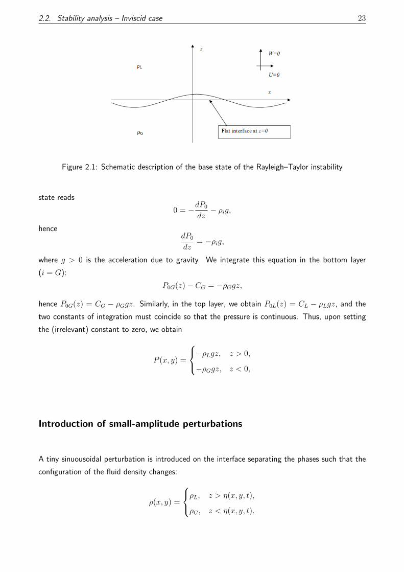
2.2. Stability analysis – Inviscid case 23
Figure 2.1: Schematic description of the base state of the Rayleigh–Taylor instability
state reads
0 = −dP0
dz− ρig,
hencedP0
dz= −ρig,
where g > 0 is the acceleration due to gravity. We integrate this equation in the bottom layer
(i = G):
P0G(z)− CG = −ρGgz,
hence P0G(z) = CG − ρGgz. Similarly, in the top layer, we obtain P0L(z) = CL − ρLgz, and the
two constants of integration must coincide so that the pressure is continuous. Thus, upon setting
the (irrelevant) constant to zero, we obtain
P (x, y) =
−ρLgz, z > 0,
−ρGgz, z < 0,
Introduction of small-amplitude perturbations
A tiny sinuousoidal perturbation is introduced on the interface separating the phases such that the
configuration of the fluid density changes:
ρ(x, y) =
ρL, z > η(x, y, t),
ρG, z < η(x, y, t).
24 Chapter 2. Rayleigh–Taylor Instability
This change induces corresponding changes in the velocity and pressure fields, to be determined now
by the relevant linearized (Euler) equations of motion:
∂
∂tui = − 1
ρi∇δpi, i = L,G,
where the perturbation velocities ui satisfy the incompressibility condition
∇ · ui = 0.
The linearized Euler equation demonstrates conservation of vorticity:
∂
∂t(∇× ui) = 0.
We assume a two-dimensional disturbance in the xz plane and project this conservation equation
on to the y-direction to obtain∂
∂t(∂xw − ∂zu) = 0.
The incompressibility condition reads (correspondingly)
∂xu+ ∂yw = 0.
Thus, we introduce a streamfunction ψ, such that u = ∂zψ and w = −∂xψ. The conservation of
vorticity equation now reads∂
∂t
(−∂2
xψi − ∂2zψi)
= 0,
or∂
∂t∇2ψi = 0,
hence ∇2ψi = Const. But the initial configuration corresponds to no flow and no vorticity, hence
∇2ψi = 0.
We make a normal-mode decomposition ψ = eikx+σtΨ(z), hence
(∂2z − k2
)Ψi = 0,
with solution
Ψi = Aie−k|z|
(the other solutions are thrown away because they correspond to unbounded disturbances as |z| →∞).

2.2. Stability analysis – Inviscid case 25
It now remains to match the streamfunction across the interface. This is where the two-phase flow
aspect of the problem enters: physical jump conditions need to be prescribed at the interface
z = η.
Jump conditions
We demand continuity of velocity at the interface z = η. In particular, wi = −ikeikx+σtΨi(z) is
continuous across the interface:
wL(x, z = η) = wG(x, z = η),
ΨL(z = η) = ΨG(z = η),
ΨL(0) +∂ΨL
∂z
∣∣0η + · · · = ΨG(0) +
∂ΨG
∂z
∣∣0η + · · · .
Linearized on to the surface z = 0, this continuity condition reads
ΨL(0) = ΨG(0).
Since Ψi = Aie−k|z|, it follows that AL = AG = A.
The other condition is the dynamic Laplace–Young condition, which says that the jump in the
normal stress across the interface must be balanced by the surface-tension force. However, the
normal stress is just −P , where P is the total pressure, P = P0 + δp. In other words, we have
PL(x, z = η)− PG(x, z = η) = γκ,
where γ is the surface tension and κ is the (mean) curvature of the interface. We now work out
each of these contributions:
• Interfacial pressure in the upper layer: We have
PL(x, z = η) = P0L(z = η) + δpL(x, z = η),
= P0L(0) +dP0L
dz
∣∣0η + δpL(x, z = 0) +
[∂
∂zδp
]z=0
η + · · · ,
= −ρLgη + δpL(x, z = 0),
where we have linearized again on to the surface z = 0.
• Interfacial pressure in the upper layer: This is similar to the upper layer, and we have
PG(x, z = η) = −ρGgη + δpG(x, z = 0),
26 Chapter 2. Rayleigh–Taylor Instability
• Mean curvature: By a standard formula, we have
κ =ηxx
(1 + η2x)
3/2.
Applying the linearization and the normal-mode decomposition, this is
κ = −k2η.
Hence, the jump condition on the pressure now reads
[−ρLgη + δpL(x, z = 0)]− [−ρGgη + δpG(x, z = 0)] = −γk2η.
This is re-arranged as
δpL − δpG = (ρL − ρG)gη − γk2η.
It remains to connect the pressure to the streamfunction and hence to write down an eigenvalue
problem.
The eigenvalue problem
We return to the perturbation equation for the u-velocity:
∂ui∂t
= − 1
ρi
∂
∂xδpi.
Going over to the normal-mode and streamfunction representations, this equation can be written as
σ∂zψ = − 1
ρiikδpi,
where ψ = eikx+σtΨ(z) is the total streamfunction. Hence,
δpi =1
kiρiσ∂zψ,
and the jump condition on the pressure can now be rewritten as
1
kiσ (ρL∂zψL − ρG∂zψG) = (ρL − ρG)gη − γk2η.
We use again the fact that ΨL = Ae−kz and ΨG = Aekz to rewrite this further as
− iσ(ρL + ρG)Aeikx+σt = (ρL − ρG)gη − γk2η, (2.1)
2.2. Stability analysis – Inviscid case 27
Let η = η0eikx+σt, where η0 is a complex number. Hence, Equation (2.1) becomes
−iσ(ρL + ρG)ψ(0) = (ρL − ρG)gη0 − γk2η0,
Some further work is needed to express η in terms of the streamfunction. We use kinematic
condition, which says that fluid particles on the interface follow the motion of the interface itself:
∂η
∂t+ u
∂η
∂x= w,
or, in a linearized version,∂η
∂t= w,
and finally, in the normal-mode and streamfunction representation,
ση0 = −ikΨ(0),
hence η0 = −ikΨ(0)/σ. Thus, the jump condition can be re-expressed as
−iσ(ρL + ρG)Ψ(0) =[(ρL − ρG)g − k2γ
][−ikΨ(0)/σ] .
Tidying up, the result is
σ2 =ρL − ρGρL + ρG
gk − γk3
ρL + ρG,
and finally,
σ =
√ρL − ρGρL + ρG
gk − γk3
ρL + ρG.
The quantity (ρL − ρG)/(ρL − ρG) > 0 is called the Atwood number:
At =ρL − ρGρL + ρG
;
the relationship between the growth rate σ and the wavenumber k is called the dispersion relation:
σ(k) =
√Atgk − γk3
ρL + ρG. (2.2)
Implications
When γ = 0 the surface tension vanishes, and the dispersion relation reads
σ(k) =√
Atgk.

28 Chapter 2. Rayleigh–Taylor Instability
Figure 2.2: Sample dispersion relation showing the bifurcation from shortwave neutral capillary wavesto longwave unstable gravitational disturbances. Model parameters: At = g = γ/(ρL + ρG) = 1.
In this case, the growth rate σ is purely real and positive, and waves of arbitrary wavelength
are unstable. In contrast, for γ 6= 0, there is a critical wavenumber k0 where the radicand in
Equation (2.2) changes sign:
Atg =γ
ρL + ρGk2
0,
such that
σ =
√
Atgk − γk3
ρL+ρG, k < k0,
±i√
γk3
ρL+ρG− Atgk, k ≥ k0,
where the long-wave (k < k0) case corresponds to pure unstable motion and the short-wave case
corresponds to neutral travelling capillary travelling waves. Thus, surface tension stabilizes short-
wave disturbances. A sample dispersion relation showing this bifurcation in the nature of the
eigensolutions is shown in Figure 2.2.
2.3 Viscous case
The base state is unchanged. The first main change is in the linearized equation of motion:
∂
∂tui = − 1
ρi∇δpi +
µiρi∇2ui, i = L,G,
which now contains a viscous term. As before, we take the curl on both sides to eliminate the
pressure:∂
∂tωi =
µiρi∇2ωi,

2.3. Viscous case 29
and we project on to the y-direction to obtain
∂
∂t(∂xw − ∂zu) =
µiρi∇2 (∂xw − ∂zu) .
As before, we introduce the streamfunction and the equation of motion reduces to
∂
∂t∇2ψ =
µiρi∇4ψ.
A normal-mode decomposition is made, such that ψ = eikx+σΨ(z), and the relevant eigenvalue
equation now reads
σ(∂2z − k2
)Ψi =
µiρi
(∂2z − k2
)4Ψi.
It is clear that the boundary conditions are
Ψi = Ψ′i = 0, as |z| → ∞.
However, we now have a fourth-order equation to match across the interface at z = 0, which requires
four matching conditioins (previously we had two matching conditions for a second-order equation).
This requires more physics.
Matching Conditions
As before, we impose continuity of velocity. Continuity of the w-component of velocity gives
ΨL(0) = ΨG(0).
We also have continuity of the u-component of velocity, where u = ∂zψ, and where ψ = eikx+σtΨ(z)
is the full streamfunction. We have
uL(x, z = η) = uG(x, z = η),
=⇒ uL(x, z = 0) = uG(x, z = 0),
=⇒ ∂zψL(x, z = 0) = ∂zψG(x, z = 0),
hence
∂zΨL(z = 0) = ∂zΨG(z = 0).
Thus, both Ψ and its first derivative are continuous across the interface.
The next condition relevant for viscous flow is the continuity of tangential stress across the
30 Chapter 2. Rayleigh–Taylor Instability
interface. Recall, the stress tensor associated with the Navier–Stokes equations is
T = −pI + µ(∇u+∇uT
),
and the tangential stress is
n · T · t,
where
t =(1, ηx)√1 + η2
x
≈ (1, ηx)
is the unit tangent vector to the interface and
n =(−ηx, 1)√
1 + η2x
≈ (−ηx, 1)
is the unit normal vector.
Now n · I · t = n · t = 0, so the tangential stress is
µn ·(∇u+∇uT
)· t = µ
2∑i,j=1
ni
(∂ui∂xj
+∂uj∂xi
)tj,
= µn1t1
(∂u1
∂x1
+∂u1
∂x1
)+mun1t2
(∂u1
∂x2
+∂u2
∂x1
)+
µn2t1
(∂u2
∂x1
+∂u1
∂x2
)+ µn2t2
(∂u2
∂x2
+∂u2
∂x2
)The only term that survives the linearization is proportional to n2t1, hence the tangential stress is
µn2t1
(∂u2
∂x1
+∂u1
∂x2
)= µ
(∂w
∂x+∂u
∂z
),
which in streamfunction form is
µ(∂2z + k2
)ψ.
Hence,
µL(∂2z + k2
)ψL = µG
(∂2z + k2
)ψG.
The final condition relevant for viscous flow is the familiar jump condition for tangential stress
across the interface. The normal stress is n ·T · n, and the jump in the normal stress is balanced
by the surface-tension force:
[n ·T · n]LG = −γκ.

2.3. Viscous case 31
We now work out the linearized normal stress. Note that
n · (pI) · n = pn · n = p.
Also, each term in the sum
n ·(∇u+∇uT
)· n =
2∑i,j=1
ninj
(∂ui∂xj
+∂uj∂xi
)
is proportional to ninj. The only contribution to survive in a linearization is i = 2 and j = 2 (with
n22 = 1)
n ·(∇u+∇uT
)· n = 2
∂w
∂z.
Thus, the linearized normal stress in the ith phase is
−pi + 2µi∂wi∂z
Thus, the final matching condition at the interface reads[−pL + 2µL
∂wL∂z
]−[−pG + 2µG
∂wG∂z
]= γk2η.
Re-arranging and using the by-now familiar streamfunction representation gives
(−pL)− (−pG)− ik (2µL∂zψL − 2µG∂zψG) = γk2η.
Now, the computation of the jump in pressures is the same as before, so we are left with the
matching condition
g (ρL − ρG) η + (−δpL + δpG)z=0 − ik (2µL∂zψL − 2µG∂zψG) = γk2η,
or
(−δpL + δpG)z=0 − ik (2µL∂zψL − 2µG∂zψG) = −g (ρL − ρG) η + γk2η.
It now remains to work out the pressure perturbation for the viscous fluid. We start with the
u-component of the velocity equation:
∂
∂tui = − 1
ρi
∂
∂xδpi +
µiρi∇2ui,
which in streamfunction-normal-mode form reads
σ∂zψ = − ik
ρiδpi +
µiρi
(∂2z − k2)∂zψ.

32 Chapter 2. Rayleigh–Taylor Instability
Hence,
ρiσ∂zψ − µi(∂2z − k2)∂zψ = −ikδpi,
and finally,
− i
kρiσ∂zψi +
i
kµi∂
3zψi − ikµi∂zψ = −δpi.
We assemble the results:
(−δpL + δpG)− 2ik (µL∂zψL − µG∂zψG)
=
(− i
kρLσ∂zψL +
i
kµL∂
3zψL − ikµL∂zψL
)−(− i
kρGσ∂zψG +
i
kµG∂
3zψG − ikµG∂zψG
)− 2ik (µL∂zψL − µG∂zψG)
=
(− i
kρLσ∂zψL +
i
kµL∂
3zψL − 3ikµL∂zψL
)−(− i
kρGσ∂zψG +
i
kµG∂
3zψG − 3ikµG∂zψG
)which is all equal to −(ρL − ρG)η + γk2η:
σ
(− i
kρL∂zψL +
i
kρG∂zψG
)+
[(i
kµL∂
3zψL − 3ikµL∂zψL
)−(
i
kµG∂
3zψG − 3ikµG∂zψ
)]= −g(ρL − ρG)η + γk2η
Multiply up by −k/i for the final result:
σ (ρL∂zψL − ρG∂zψG) +[(
3k2µL∂zψL − µL∂3zψL
)−(3k2µG∂zψG − µG∂3
zψG)]
= −ik[(ρL − ρG)− γk2
]η. (2.3)
Now, if we used the kinematic condition here to write η = −ikψ(0)/σ, we would end up with σ2 in
the matching condition. This is not advisable: we want a linear eigenvalue problem in the variable
σ. Therefore, we leave Equation (2.3) as-is, and include η as an extra variable. Let us assemble the
results here. We have the following ordinary differential equations in the eigenvalue σ valid in the
bulk parts of the domain:
σρL(∂2z − k2
)ΨL = µL
(∂2z − k2
)2ΨL, z > 0, (2.4a)
σρG(∂2z − k2
)ΨG = µG
(∂2z − k2
)2ΨG, z < 0. (2.4b)

2.3. Viscous case 33
The following matching conditions apply at z = 0:
ΨL(0) = ΨG(0), (2.4c)
∂zΨL(0) = ∂zΨG(0), (2.4d)
µL(∂2z + k2
)ΨL = µG
(∂2z + k2
)ΨG, (2.4e)
σρL∂zΨL + µL(3k2∂zΨL − µL∂3
zΨL
)= σρG∂zΨG + µG
(3k2∂zΨG − ∂3
zΨG
)−ik
[g(ρL − ρG)k − γk3
]η0. (2.4f)
Here, again, η = η0eikx+σt and η0 is the phase, determined by the kinematic condition
ση0 = −ikΨ(0). (2.4g)
Finally, the following boundary conditions apply:
ψL, ∂zψL → 0 as z →∞, ψG, ∂zψG → 0 as z → −∞. (2.4h)
These are the equations we now solve. Although it is possible to solve these equations semi-
analytically, it is in fact more revealing (and easier) to solve them numerically. We introduce a
convenient numerical method in the next chapter – numerical spectral methods.
Exercise 2.1 Rayleigh–Taylor instability in a porous medium: Consider the stability of
a basic flow in which two incompressible fluids move with a horizontal interface and uniform
vertical velocity in a uniform porous medium. You are given that motion of a fluid in a porous
medium is governed by Darcy’s Law, namely that u = ∇φ, where φ = −k(p+ gρz)/µ, ρ is the
density and µ the dynamic viscosity of the fluid, and k is the permeability of the medium to the
fluid.
Let the lower fluid have density ρ1 and viscosity µ1 and the upper fluid ρ2 and µ2; let the medium
have permeability k1 to the lower and k2 to the upper fluid, and let the basic velocity be W z.
Then show that the flow is stable if and only if(µ1
k1
− µ2
k2
)W + g(ρ1 − ρ2) ≥ 0.
Hints: Decompose the velocity potential in each phase as φi + δφi, where φi is the base-state
contribution. Use (and prove) the following intermediate steps if necessary:
• ∇2φi = ∇2δφi = 0 in the interior of each fluid domain.

34 Chapter 2. Rayleigh–Taylor Instability
• Write δφi = eλt+iαxΦi, hence (∂2z − α2)Φi = 0.
• Continuity of normal velocity across the perturbed interface at z = η(x, t) = η0eλt+iαx
implies Φ1 = Aeαz and Φ2 = −Ae−αz. Also, obtain the kinematic condition λη0 = Aα.
• Continuity of pressure across the perturbed interface implies that(∂p1
∂z− ∂p2
∂z
)η =
µ1
k1
δφ1 −µ2
k2
δφ2.
Exercise 2.2 Rayleigh–Taylor stability of superposed fluids confined in a vertical cylin-
der: Consider an inviscid incompressible fluid of density ρ1 at rest beneath a similar fluid of
density ρ2, the fluids being confined by a long vertical rigid cylinder with equation r = a and
there being surface tension γ at the interface with equation z = 0. Here cylindrical polar co-
ordinates (r, θ, z) are used and Oz is the upward vertical. Then show, much as in the analysis
throughout this chapter, that small irrotational disturbances of the state of rest may be found
in terms of the normal modes of the form
φ = cosnθJn(kr)e−k|z|+λt,
where φ is the velocity potential of the disturbance, n = 0, 1, 2, · · · , and where
λ2 =g(ρ2 − ρ1)k − γk3
ρ1 + ρ2
.
Here, the wavenumber k is determined by the condition that ka equals the mth positive zero
j′n,m of the derivative J ′n of the Bessel function for m = 1, 2, · · · . Deduce that there is stability
if
a2g(ρ2 − ρ1) < γj21,1.

Chapter 3
Spectral methods in fluid dynamics
3.1 Overview
We introduce numerical spectral methods in the context of a simple two-point boundary-value
problem. We then extend the method to the problem of determining the eigenvalues of the viscous
Rayleigh–Taylor problem. The following books might help in understanding this last chapter:
• Chebyshev and Fourier spectral methods, J. P. Boyd, Dover Publications (2000). Boyd himself
has put a copy of this on his website and is therefore available for free in pdf form [Boy01].
• Spectral methods in Matlab, L. N. Trefethen, SIAM Publications (2001) [TTTD93].
3.2 A simpler problem
Consider the equationd2f
dy2= −λf, y ∈ [−L/2, L/2] , (3.1)
which is to be solved with vanishing boundary conditions
f(−L/2) = f(L/2) = 0.
This is an eigenvalue problem in the eigenvalue λ. However, we already know the solution: it is
f(y) = fn(y) = sin(√λny), λn =
4π2
L2n2, n = 1, 2, · · ·
or
f(y) = fn(y) = cos(√λny), λn =
4π2
L2
(n+ 1
2
)2, n = 0, 1, · · ·
35

36 Chapter 3. Spectral methods in fluid dynamics
where the apparently free parameter λ is now forced to take discrete values, λ = λn.
We are now going to ‘shoot a pigeon with a cannon’, and solve this problem numerically. We are
going to expand the solution in terms of a set of basis functions,
f(y) =∞∑n=0
anTn(x), x =2
Ly,
where Tn(x)∞n=0 are a complete set of basis functions on the interval [−1, 1] called the Chebyshev
polynomials:
Tn(x) = cos(n arccos(x)).
Although this does not really look like a polynomial in x, it is!. The first few are shown here:
T0(x) = 1,
T1(x) = x,
T2(x) = 2x2 − 1,
T3(x) = 4x3 − 3x,
T4(x) = 8x4 − 8x2 + 1.
For more information on the properties of these functions, you may, in this instance, check out the
Wikipedia article. I can personally vouch for this article since I have contributed to it myself!
Just as 1, sin
(2nπ
Lx
), cos
(2nπ
Lx
)∞n=1
are a good set of basis functions for periodic functions on an interval [−L/2, L/2], so too are
the Chebyshev polynomials for arbitrary functions on the same interval. Thus, we in expanding
the solution in terms of these exotic functions, instead of familiar sines and cosines, we are taking
into account the fact that the solution is not necessarily periodic. Of course, we must truncate the
expansion in a numerical framework, so we work with the approximate solution
fN(y) =N∑n=0
anTn(x).
There are N+1 undetermined coefficients and two boundary conditions. That leaves N−1 conditions
to obtain. We therefore evaluate the ODE at N − 1 interior points to give N + 1 constraints on

3.2. A simpler problem 37
the coefficients:
fN(−L/2) = 0,
d2fNdy2
∣∣∣y1
= −λfN(y1),
......
d2fNdy2
∣∣∣yN−1
= −λfN(yN−1),
fN(+L/2) = 0,
or
N∑n=0
anTn(−1) = 0,
N∑n=0
an
(2
L
)2
T ′′n (x1) = −λN∑n=0
anTn(x1),
......
N∑n=0
an
(2
L
)2
T ′′n (xN−1) = −λN∑n=0
anTn(xN−1),
N∑n=0
anTn(+1) = 0.
The interior points are NOT arbitrary: we evaluate at the N − 1 points
x1, x2, · · · , xN−1 = cos( πN
), cos
(2π
N
), · · · , cos
((N − 1)
π
N
);
these are the collocation points.
But now we have a generalised eigenvalue problem:
La = λMa,
where
L =
T0(−1) · · · TN(−1)
(2/L)2T ′′0 (x1) · · · (2/L)2T ′′N(x1)...
...
(2/L)2T ′′0 (xN−1) · · · (2/L)2T ′′N(xN−1)
T0(+1) · · · TN(+1)
,
38 Chapter 3. Spectral methods in fluid dynamics
M = −
0 · · · 0
T0(x1) · · · TN(x1)...
...
T0(xN−1) · · · TN(xN−1)
0 · · · 0
,
and
a = (a0, · · · , an)T .
This is a standard problem, and can be solved using a numerical package, such as ‘eig’ in Matlab.
• Typing
d=eig(L,M);
in Matlab yields the first N + 1 eigenvalues.
• We must then check that the eigenvalues are real (a check for bugs in the code):
plot(imag(d),’o’)
• Having done that, we sort the eigenvalues in increasing order:
d=sort(d);
• Then, we plot the results.
plot(d,’o’)
• Typically, the solver yields an accurate answer only for the first few eigenvalues. Suppose
we want to find the first two eigenvalues accurately. We fix N and compute the first two
eigenvalues. We then increase N and compute the eigenvalues again. We continue increasing
N until the first two eigenvalues do not change upon varying N . The solver is then said to
have converged.
Happily, these solvers such as ‘eig’ tell us the eigenvectors as well as the eigenvalues. Typing
[V,D]=eig(L,M);
gives two (N+1)×(N+1) matrices. The matrix D is diagonal and corresponds to the eigenvalues,
3.2. A simpler problem 39
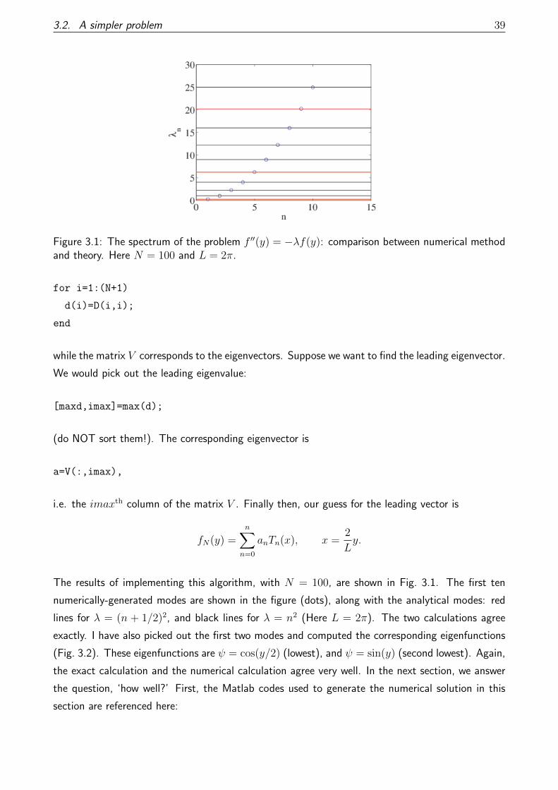
Figure 3.1: The spectrum of the problem f ′′(y) = −λf(y): comparison between numerical methodand theory. Here N = 100 and L = 2π.
for i=1:(N+1)
d(i)=D(i,i);
end
while the matrix V corresponds to the eigenvectors. Suppose we want to find the leading eigenvector.
We would pick out the leading eigenvalue:
[maxd,imax]=max(d);
(do NOT sort them!). The corresponding eigenvector is
a=V(:,imax),
i.e. the imaxth column of the matrix V . Finally then, our guess for the leading vector is
fN(y) =n∑n=0
anTn(x), x =2
Ly.
The results of implementing this algorithm, with N = 100, are shown in Fig. 3.1. The first ten
numerically-generated modes are shown in the figure (dots), along with the analytical modes: red
lines for λ = (n + 1/2)2, and black lines for λ = n2 (Here L = 2π). The two calculations agree
exactly. I have also picked out the first two modes and computed the corresponding eigenfunctions
(Fig. 3.2). These eigenfunctions are ψ = cos(y/2) (lowest), and ψ = sin(y) (second lowest). Again,
the exact calculation and the numerical calculation agree very well. In the next section, we answer
the question, ‘how well?’ First, the Matlab codes used to generate the numerical solution in this
section are referenced here:

40 Chapter 3. Spectral methods in fluid dynamics
(a) (b)
Figure 3.2: The first two eigenfunctions of the problem f ′′(y) = −λf(y). Here N = 100 andL = 2π.
• Calculation of eigenvalues: simple.m
• Calculation of eigenfunctions: make eigenfunction simple
Exercise 3.1
1. Solve the eigenvalue problem (3.1) analytically, this time with the Neuman boundary
conditions
f ′(−L/2) = f ′(L/2) = 0.
2. Modify the Matlab codes above to solve the eigenvalue problem above in (1) numerically.
Compare the analytical and numerical results, both for the eigenfunctions and eigenvalues.
3.3 Exponential convergence
In this section we examine some numerical issues surrounding the Chebyshev collocation method.
So far we have been quite casual in our use of nomenclature. For definiteness, we work on the
interval [−1, 1]. We start with the operator problem
Lf = λMf,

3.3. Exponential convergence 41
and construct the approximate solution
f(y) ≈ fN(y) =N∑n=0
anTn(x), x ∈ [−1, 1] .
Until now, we have called this a truncation, although really it is an interpolation. Let’s see why
the latter label is more appropriate.
First, recall the following result, due to Lagrange:
Theorem 3.1 Let f(x) be some function whose value is known at the discete points x0, x1, · · · , xN .
Then there exist polynomials C0(x), C1(x), · · · , CN(x) such that the function
PN(x) =N∑i=0
f(xi)Ci(x)
agrees with f(x) at the points x0, x1, · · · , xN :
PN(xi) = f(xi), i = 0, 1, · · · , N.
Proof: Take
Ci(x) =N∏
j=0,j 6=i
x− xjxi − xj
.
Noting that
Ci(xk) = δik,
the result follows. This result establishes the existence of interpolating polynomials, but does not
tell us which ones are best. It turns out that the Chebyshev polynomials are among the better
polynomials, and that the non-uniform Chebyshev grid is best. In what follows, we explain why.
For illustration purposes, consider the problem Lf = λMf where boundary conditions are not
important. We pose the interpolation approximation
fN(x) = 12b0T0(x) +
N−1∑n=1
bnTn(x) + 12bNTN(x)
We impose the condition that fN(x) and f(x) agree exactly at the points x0, x1, · · · , xN . We do
not know the value of f(x), but we do know the differential equation it solves. Thus, we have
LfN(xk) = λMfN(xk), k = 0, 1, · · ·N.
Then the following theorem holds:

42 Chapter 3. Spectral methods in fluid dynamics
Theorem 3.2 Let the interpolation grid be given by
xk = cos(kπ/N), k = 0, 1, · · ·N.
Let fN(x) be the interpolating polynomial of degree N which interpolates to f(x) on this grid:
fN(x) = 12b0T0(x) +
N−1∑n=1
bnTn(x) + 12bNTN(x),
fN(xk) = f(xk)
Finally, let αnn be the coefficients of the exact expansion of f(x) in Chebyshev polynomials:
f(x) = 12α0T0(x) +
∞∑n=1
αnTn(x)
Then,
bn =2
N
[12f(x0)Tn(x0) +
N−1∑k=0
f(xk)Tn(xk) + 12f(xN)Tn(xN)
],
which leads to the following bound:
|f(x)− fN(x)| ≤ 2∞∑
n=N+1
|αn|.
The proof of this theorem is straightforward but the reader is referred to Boyd [Boy01] for the
details. We focus instead on the following corollary.
Theorem 3.3 If the problem Lf = λMf is analytic, then the convergence of the interpolation
approximation in Theorem 3.2 is exponential.
Proof: If there are no singularities in the problem Lf = λMf , then a power-series solution is
possible, with finite radius of convergence. Continuing the power series into the complex plane gives
a solution that has derivatives of all order. Thus, we may assume that
|f (p)(x)| ≤Mp,
where the bound is independent of x ∈ [−1, 1].
Next, we note that a Chebyshev series is but a Fourier series in disguise! For, let θ = arccos(x).
Then,
f(x) = 12α0 +
∞∑n=1
αnTn(x) = 12α0 +
∞∑n=1
αn cos(nθ).
3.3. Exponential convergence 43
Differentiating both sides p times with respect to θ gives
∞∑n=1
αnnp<(ipeinθ
)=dpf
dθp.
But note:
df
dθ=
dx
dθ
df
dx= − sin θ
df
dx,
d2f
dθ= sin2 θ
d2f
dx2− cos θ
df
dx,
and so on, implying that |dpf/dθp| ≤ Mp, where the bound is independent of θ or x. Hence,∣∣∣∣∣∞∑n=0
αnnp<(ipeinθ
)∣∣∣∣∣ ≤ Mp,
and this is a convergent series. It follows that the general term tends to zero:
limn→∞
|αn|np = 0.
At worst,
|αn| ≤ A′e−γ′nδ , n→∞,
for some positive parameters A′, γ′, and δ that are independent of n. Consider log |αn|/n as n→∞;
this is
log |αn|/n ∼ −γnδ−1, with R = limn→∞
log |αn|/n.
Three possibilities emerge:
1. R = ∞, corresponding to δ > 1 and supergeometric behaviour. This implies that the true
analytic eigensolution is an entire function in the complex plane (analytic continuation);
2. R = Const, corresponding to δ = 1 and geometric behaviour. This implies that the true
analytic eigensolution that is a meromorphic in the complex plane got by analytically continuing
the real solution, or has branch cuts, where these singularties are far from the (real) interval
of interest.
3. R = 0, corresponding to subgeometric behaviour.
In any case, given the assumed regularity of the ODE to be solved, only cases 1 and 2 pertain, and
thus, in a worst-case sceario, we have the geometric case, so we can conclude that for the problems
of interest,
|αn| ≤ Ae−γn, n→∞,

44 Chapter 3. Spectral methods in fluid dynamics
for some further positive parameters A and γ that are independent of n. Hence, there exists N0 ∈ Nsuch that
|αn| < Ae−γn, for all n > N0.
Returning to the bound in the Theorem 3.2, we have
|f(x)− fN0(x)| ≤ 2∞∑
n=N0+1
|αn|,
≤ 2A∞∑
n=N0+1
e−γn,
≤ 2Ae−γ(N0+1)
∞∑r=0
e−γr,
≤ Be−γN0
The error is thus proportional to e−γN0 and we therefore say that the Chebyshev collocation method
converges exponentially. Typically, this result generalizes to situations where the boundary con-
ditions are built in to the interpolation coefficients.
3.4 The Rayleigh–Taylor instability revisited
I have implemented a numerical spectral method for the computation of the eigenvalues of the
Rayleigh–Taylor instability. The eigenvalue problem is solved in a finite domain z ∈ [−H,H]. In
numerical methods, it is convenient to nondimesnionalize the problem. The curious thing about the
Rayleigh–Taylor problem is that there is no natural unit of length, and even in the finite domain, using
the scale H as the standard lengthscale is problematic. Thus, we introduce an arbitrary lengthscale
h0 and non-dimesnionalize with respect to that, as well as the typical velocity scale U0 =√gh0.
Densities and viscosities are scaled relative to the bottom-layer density and viscosity – ρG and µG
respectively. The non-dimensional problem to solve reads
σrL(∂2z − k2
)ΨL =
mL
Re
(∂2z − k2
)2ΨL, z ∈ (0, νL), (3.2a)
σrG(∂2z − k2
)ΨG =
mG
Re
(∂2z − k2
)2ΨG, z ∈ (−νG, 0). (3.2b)
3.4. The Rayleigh–Taylor instability revisited 45
The following matching conditions apply at z = 0:
ΨL(0) = ΨG(0), (3.2c)
∂zΨL(0) = ∂zΨG(0), (3.2d)
mL
(∂2z + k2
)ΨL = mG
(∂2z + k2
)ΨG, (3.2e)
σrL∂zΨL +mL
Re
(3k2∂zΨL − ∂3
zΨL
)= σrG∂zΨG +
mG
Re
(3k2∂zΨG − ∂3
zΨG
)−ik
[(rL − rG)k − Sk3
]η0. (3.2f)
Here, η = η0eikx+σt and η0 is the phase, determined by the kinematic condition
ση0 = −ikΨ(0). (3.2g)
Finally, the following boundary conditions apply:
ψL, ∂zψL → 0 as z →∞, ψG, ∂zψG → 0 as z → −∞. (3.2h)
The dimensionless quantities are defined here as follows. First, we have νL = νG = H/h0 ∈ (0,∞),
which are variable parameters. For the densities, we have
rL = ρL/ρG ∈ [1,∞), rG = ρG/ρG = 1,
For the viscosity parameters, we have
mL = µL/µG ∈ [0,∞), mG = µG/µG = 1,
The Reynolds number is Re = U0h0ρG/µG, also variable. Finally, S = γ/(ρGhU20 ) is a dimensionless
surface-tension parameter.
It is not necessary for the students to write a code to solve the RTI eigenvalue problem (I have done
that already). Instead, you can take the codes
• OS rti.m
• call OS rti.m
and study them yourself. In particular, carry out the following exercise:
Exercise 3.2 Take the RTI eigenvalue solver. Take Re = 1000 and mL = mG = 1. Choose
further appropriate values for the other parameters. Show in this parameter regime of large

46 Chapter 3. Spectral methods in fluid dynamics
Figure 3.3: Comparison between the inviscid theory and the numerical method
Reynolds number that the numerical results agree very closely with the earlier inviscid analysis.
Justify this finding.
Example: With Re = 1000, mL = mG = 1, νL = νG = 2, NL = NG = 100 and S = 0 the
results in Figure 3.3 were obtained. Excellent agreement is obtained. The small discrepancies at
long wavelengths (small α) have been investigated by an M.Sc. student and are found to arise due
to the confinement of the numerical domain.
Chapter 4
Stability of viscous parallel flow
Overview
We introduce the Orr–Sommerfeld equation for the stability of parallel flow. We demonstrate
one particular instance where exact solutions for the eigenvalue problem are obtainable. We then
pass over to numerical spectral methods to calculate the critical Reynolds number for the onset of
instability in Poiseuille channel flow.
4.1 Parallel flow
We consider the Navier–Stokes equations for a wall-bounded flow, such that z ∈ [0, H], and such
that the velocity vanishes at z = 0 and z = H (no-slip). Suppose that the flow is characterized by
a typical velocity V . The Navier–Stokes equations then non-dimensionalize in a standard fashion:
∂u
∂t+ u · ∇u = −∇p+
1
Re∇2u, ∇ · u = 0, (4.1a)
where u and p have their usual meanings and
Re =V Hρ
µ(4.1b)
is the (dimensionless) Reynolds number. Here, ρ and µ are the fluid density and viscosity respectively.
We henceforth work with these non-dimensional equations of motion.
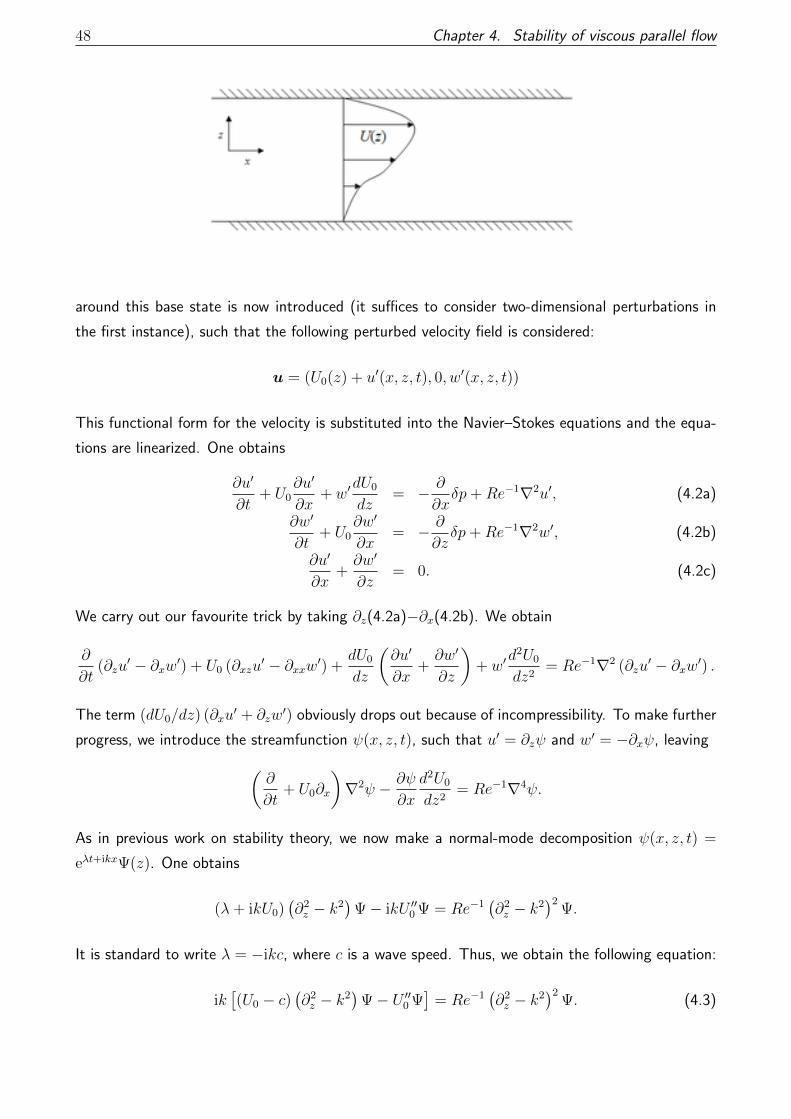
Consider now a parallel flow U0(z) shown schematically in Figure 4.1. The origin of such a flow
profile will be discussed in later sections in this chapter. For now, it suffices to notice that a flow u =
(U0(z), 0, 0) is an equilibrium solution of the Navier–Stokes equation (4.1a). A small perturbation
47
48 Chapter 4. Stability of viscous parallel flow
around this base state is now introduced (it suffices to consider two-dimensional perturbations in
the first instance), such that the following perturbed velocity field is considered:
u = (U0(z) + u′(x, z, t), 0, w′(x, z, t))
This functional form for the velocity is substituted into the Navier–Stokes equations and the equa-
tions are linearized. One obtains
∂u′
∂t+ U0
∂u′
∂x+ w′
dU0
dz= − ∂
∂xδp+Re−1∇2u′, (4.2a)
∂w′
∂t+ U0
∂w′
∂x= − ∂
∂zδp+Re−1∇2w′, (4.2b)
∂u′
∂x+∂w′
∂z= 0. (4.2c)
We carry out our favourite trick by taking ∂z(4.2a)−∂x(4.2b). We obtain
∂
∂t(∂zu
′ − ∂xw′) + U0 (∂xzu′ − ∂xxw′) +
dU0
dz
(∂u′
∂x+∂w′
∂z
)+ w′
d2U0
dz2= Re−1∇2 (∂zu
′ − ∂xw′) .
The term (dU0/dz) (∂xu′ + ∂zw
′) obviously drops out because of incompressibility. To make further
progress, we introduce the streamfunction ψ(x, z, t), such that u′ = ∂zψ and w′ = −∂xψ, leaving(∂
∂t+ U0∂x
)∇2ψ − ∂ψ
∂x
d2U0
dz2= Re−1∇4ψ.
As in previous work on stability theory, we now make a normal-mode decomposition ψ(x, z, t) =
eλt+ikxΨ(z). One obtains
(λ+ ikU0)(∂2z − k2
)Ψ− ikU ′′0 Ψ = Re−1
(∂2z − k2
)2Ψ.
It is standard to write λ = −ikc, where c is a wave speed. Thus, we obtain the following equation:
ik[(U0 − c)
(∂2z − k2
)Ψ− U ′′0 Ψ
]= Re−1
(∂2z − k2
)2Ψ. (4.3)
4.2. Couette flow 49
Equation (4.3) is the celebrated Orr–Sommerfeld equation. When supplemented with the no-slip
boundary conditions
Ψ(0) = Ψ′(0) = Ψ(1) = Ψ′(1)
it is an eigenvalue problem in the eigenvalue c.
4.2 Couette flow
Consider again the two parallel plates in Figure 4.1. Suppose that the upper plate moves at a
constant velocity V . We work out the base state of the Navier–Stokes equations in this instance:
simply
∇2u = 0,
with u = (U0, 0, 0) for a parallel flow, hence d2U0/dz2 = 0, hence U0 = A + Bz. The no-slip
condition at the lower wall gives A = 0. Now, at the upper wall, no slip means ‘no relative motion’:
the plate and the fluid-at-the-plate should move at exactly the same velocity, hence U0(H) = V ,
hence BH = V , hence
U0(z) = zV/H.
This is the celebrated Couette flow. Going over to non-dimensional variables, this is simply U0 = z,
and the corresponding Orr–Sommerfeld equation reads
ik (z − c)(∂2z − k2
)Ψ = Re−1
(∂2z − k2
)2Ψ. (4.4)
Analytical progress can be made with respect to Equation (4.4). Call v = (∂2z − k2) Ψ. Then, we
are left with the equation
ik (z − c) v = Re−1(∂2z − k2
)v. (4.5)
Certainly, the trivial solution is a possibility for Equation (4.5), leaving v = (∂2z − k2) Ψ = 0, hence
Ψ = cosh(kz), Ψ = sinh(kz).
However, because the eigenvalue equation is fourth order, two other linearly independent solutions
can be found. We re-write Equation (4.5) as
d2v
dz2−Reik
(z − c− ik
Re
)v = 0.

50 Chapter 4. Stability of viscous parallel flow
Let z = z − c− ik/Re. Hence, we obtain
d2v
dz2−Reikzv = 0.
Introduce ξ = λz, where λ is constant. We have
d
dz=dξ
dz
d
dξ.
Hence,
λ2d2v
dξ2− ikRe
λξv = 0.
Choosing λ3 = ikRe gives Airy’s equation:
d2v
dξ2− ξv = 0,
with solutions
v = Ai(ξ), v = Bi(ξ).
We also choose the particular cube root of i1/3 = eiπ/6.
We must now solve the equations
(∂2z − k2)Ψ = Ai(ξ), (∂2
z − k2)Ψ = Bi(ξ). (4.6)
These are linear second-order inhomogeneous equations. We use the method of variation of param-
eters. We study first the solutions of the homogeneous problem
Ψ1(z) = cosh(kz), Ψ2(z) = sinh(kz).
Let’s focus for definiteness on the case where the right-hand side is Ai(ξ). We construct the
Wronskian
W (z) =
∣∣∣∣∣ Ψ1(z) Ψ2(z)
Ψ′1(z) Ψ′2(z)
∣∣∣∣∣ =
∣∣∣∣∣ cosh(kz) sinh(kz)
k sinh(kz) k cosh(kz)
∣∣∣∣∣ ,which gives W (z) = k. Next, we form the Wronskians Wi(z), which is identical to W (z) except
that the ith column is replaced by (0, Ai(ξ))T . We have
W1(z) =
∣∣∣∣∣ 0 sinh(kz)
Ai(ξ) k cosh(kz)
∣∣∣∣∣ = − sinh(kz)Ai(ξ).

4.2. Couette flow 51
Also,
W2(z) =
∣∣∣∣∣ 0 sinh(kz)
k cosh(kz) Ai(ξ)
∣∣∣∣∣ = cosh(kz)Ai(ξ).
The particular integral in the method of variation-of-parameters by given by
Ψ =2∑i=1
Ψi(z)
∫Wi(z
′)
W (z′)dz.
Hence,
Ψ =1
k
[− cosh(kz)
∫sinh(kz′)Ai(ξ)dz′ + sinh(kz)
∫cosh(kz′)Ai(ξ)dz′
].
Using a trigonometric identity here, this becomes
Ψ =1
k
∫sinh[k(z − z′)]Ai(ξ)dz′.
Finally, we call this solution ξ1(z) and we fill in for ξ:
χ1(z) =1
k
∫ z
0
sinh[k(z − z′)]Ai[(ikRe)1/3
(z′ − c− ik
Re
)]dz′,
Here, the limits of integration have been chosen such that χ1(0) = χ′1(0) = 0, such that χ1(z)
satisfies the boundary conditions at z = 0. A similar trick can be performed when the right-hand
side of Equation (4.6) is equal to Bi(ξ), one obtains the solution χ2(z), where
χ2(z) =1
k
∫ z
0
sinh[k(z − z′)]Bi[(ikRe)1/3
(z′ − c− ik
Re
)]dz′,
with χ2(0) = χ′2(0) = 0.
We have the following solution of the eigenvalue problem:
Ψ = AΨ1(z) +BΨ2(z) + Cχ1(z) +Dχ2(z).
The vanishing of the streamfunction at the boundaries implies that∣∣∣∣∣∣∣∣∣∣1 0 0 0
0 k 0 0
cosh(k) sinh(k) χ1(1) χ2(1)
k sinh(k) k cosh(k) χ′1(1) χ′2(1)
∣∣∣∣∣∣∣∣∣∣= 0.
52 Chapter 4. Stability of viscous parallel flow
This determinant problem simplifies dramatically to
k [χ1(1)χ′2(1)− χ2(1)χ′1(1)] = 0. (4.7)
The right-hand side can be viewed as a complex-valued function of k, Re, and c (the latter a complex
variable). We therefore have the condition
F (k,Re, c) = 0,
which is a rootfinding condition, with a set of roots cn(k,Re) such that F (k,Re, cn) = 0.
Analytical progress based on Equation (4.7) is difficult if not impossible [DR81]. Indeed, there is
a celebrated theorem due to Romanov [Rom73] that states that ci(k,Re) ≤ 0 for all finite real
values of k and Re, indicating the unconditional linear stability of plane Couette flow. However,
this theorem uses a completely different approach in the proof, and the dispersion relation (4.7) is
therefore something of a dead end. Therefore, in a later part of this chapter, we introduce numerical
spectral methods for solving the generic Orr–Sommerfeld equation.
4.3 Poiseuille flow
Consider the two parallel plates in Figure 4.1. Suppose now that both plates are stationary but that
a constant pressure drop dP/dL < 0 is applied along the length of the channel We work out the
base state of the Navier–Stokes equations in this instance:
0 = −dPdL
+ µ∇2u,
0 = ∇2w.
We assume only a z-dependence for the velocity, giving d2w/dz2 = 0, with w(0) = w(H) = 0,
hence w = 0. Thus, the equations to solve reduce to
−dPdL
+ µd2U0
dz2= 0,
where the base state in the streamwise (x-direction) is denoted now by U0(z). The equation is
integrated twice to yield
U0 = A+Bz +1
2µ
dP
dLz2.
The no-slip condition at the lower wall gives A = 0. At the upper wall z = H, the same condition
gives
B = − 1
2µ
dP
dLH,

4.3. Poiseuille flow 53
hence
U0 = − 1
2µ
dP
dL
(zH − z2
).
This is tidied up slightly here to give
U0 =H2
2µ
∣∣∣∣dPdL∣∣∣∣ [ zH − ( zH)2
].
As before, it is necessary to introduce a velocity scale V , and to nondimensionalize the problem
based on the scales V and H. We choose V to be the so-called friction velocity,
ρV 2 = µdU0
dz
∣∣z=0
,
hence
ρV 2 =1
2
∣∣∣∣dPdL∣∣∣∣H =⇒ V =
√H
2ρ
∣∣∣∣dPdL∣∣∣∣.
Introduce also z = z/H, such that the base-state velocity profile reads
U0 =H2
2µ
∣∣∣∣dPdL∣∣∣∣ [ zH − z
H
2].
We have
U0 =U0
V,
=
H2
2µ
∣∣dPdL
∣∣ (z − z2)√H2ρ
∣∣dPdL
∣∣ ,
=
ρHµ
H2ρ
∣∣dPdL
∣∣ (z − z2)√H2ρ
∣∣dPdL
∣∣ ,
=ρH
µ
√H
2ρ
∣∣∣∣dPdL∣∣∣∣ (z − z2
),
=ρV H
µ
(z − z2
),
= Re∗(z − z2
),
where
Re∗ =ρV H
µ
54 Chapter 4. Stability of viscous parallel flow
is the Reynolds number based on the friction velocity and the channel depth H. We now omit all
ornamentation over the dimensionless variables and write down the Orr–Sommerfeld equation
ik[(U0 − c)
(∂2z − k2
)− U ′′0
]Ψ = Re−1
∗(∂2z − k2
)2Ψ, U0(z) = Re∗z(1− z). (4.8)
It is now of pressing urgency to introduce a numerical method to obtain a reliable solution of both
Equation (4.8) for the Poiseuille problem, but also to illuminate the dispersion relation of the Couette
flow problem in Equation (4.4). We do this in the next section.
4.4 Spectral methods for the generic Orr–Sommerfeld equa-
tion
We start with the generic Orr–Sommerfeld equation
ik[(U0 − c)
(∂2z − k2
)− U ′′0
]Ψ = Re−1
∗(∂2z − k2
)2Ψ, z ∈ (0, 1), (4.9)
together with the necessary boundary conditions
Ψ(z) = Ψ′(z) = 0, z = 0, 1.
A trial solution
ΨN(z) =N∑i=0
AnTn(η)
is made, with η = 2z − 1, such that η = 0 and η = 1 denote the boundaries. This is substituted
into Equation (4.9):
N∑n=0
An
ik[(U0 − c)
(∂2z − k2
)− U ′′0
]Tn(η)
= Re−1
N∑n=0
An(∂2z − k2
)2Tn(η) (4.10)
This equation is now evaluated at N − 4 collocation points
ηj = cos
(πj
N − 3
), j = 1, · · · , N − 3

4.4. Spectral methods for the generic Orr–Sommerfeld equation 55
and the following set of equations is obtained:
λ
N∑j=0
Aj[s2T ′′n (ηj)− k2Tn(ηj)
]+
ikN∑j=0
Aj[s2U0(zj)T
′′n (ηj)− k2U0(zj)Tn(ηj)− U ′′0 (zj)Tn(ηj)
]= Re−1
N∑n=0
An[s4T (iv)
n (ηj)− 2k2s2T 2n(ηj) + k4Tn(ηj)
], (4.11)
where s = dη/dz = 2 and zj = 2ηj − 1. We now introduce a number of matrices:
d0Tij = Tj(ηi),
d2Tij = s2T ′′j (ηi),
d4Tij = s4T(iv)j (ηi),
d0Td0Uij = U0(zi)Tj(ηi),
d0Td2Uij = U ′′0 (zi)Tj(ηi),
d2Td0Uij = s2U0(zi)T′′j (ηi),
A = (A0, · · · , AN)T ,
such that Equation (4.11) can now be written in matrix form as follows:
λ(d2T− k2d0T
)A = −ik
(d2Td0U− k2d0Td0U− d0Td2U
)A
+Re−1(d4T− 2k2d2T + k4d0T
)A.
However, since i = 0, 1, · · · , N − 3 and j = 1, 2, · · ·N + 1, this equation set is not complete (four
rows are missing). We now impose the boundary conditions. ΨN(0) = 0 implies that
N∑j=0
Tj(−1)Ai = 0.
Similarly, Ψ′N(0) = 0 implies thatN∑j=0
T ′j(−1)Aj = 0.

56 Chapter 4. Stability of viscous parallel flow
and so on for the other boundary conditions. Thus, we now form a new linear problem:
λ
0 0 · · · 0
0 0 · · · 0
d2T− k2d0T
0 0 · · · 0
0 0 · · · 0
A
=
T0(−1) T1(−1) · · · TN(−1)
T ′0(−1) T1; (−1) · · · T ′N(−1)
−ik (d2Td0U− k2d0Td0U− d0Td2U)
+Re−1 (d4T− 2k2d2T + k4d0T)
T0(1) T1(1) · · · TN(1)
T ′0(1) T ′1(1) · · · T ′N(1)
A
or in a more abstract notation,
λMA = LA, (4.12)
which is now a straightforward finite-dimensional generalized-eigenvalue problem that can be solved
in Matlab (or any other linear algebra package). Obviously, the number of Chebyshev polynomials
N should be adjusted until numerical convergence is achieved.
Couette flow
Equation (4.12) is solved for U0(z) = z for various Reynolds numbers in the range Re = 100 up to
Re = 100, 000, and in each instance N = 100 is sufficient for convergence. The results are shown
in Figure 4.1 confirming (but by no means proving) the stability of Couette flow to infinitesimal
disturbances.
Poiseiulle flow
Equation (4.12) is solved for U0(z) = Re∗z(1−z) and the results shown in Figure 4.2 for Re∗ = 100
and Re∗ = 1000. It can be seen that for the lower Reynolds number the flow is stable at all
wavenumbers, while for Re∗ = 1000, there is a range of wavenumbers within which the flow is

4.4. Spectral methods for the generic Orr–Sommerfeld equation 57
Figure 4.1: Numerically-generated dispersion relation for Couette flow for range of different Reynoldsnumbers. Solid line: Re = 100. Dashed line: Re = 1000. Dotted line: Re = 10, 000. Dot-dashedline: Re = 100, 000. It can be seen that the disturbances become less stable as Re increases butthe curve corresponding to the growth rate never crosses the horizontal axis, which underscoresthe analytical result that Couette flow is stable to infinitesimal disturbances at all finite Reynoldsnumbers.
Figure 4.2: Numerically-generated dispersion relation for Poiseuille flow for range of differentReynolds numbers. Solid line: Re = 1000, linearly unstable. Dotted line: Re = 100, linearlystable. In each instance N = 100 is sufficient for convergence.

58 Chapter 4. Stability of viscous parallel flow
unstable. This therefore suggests a critical Reynolds number Re∗c at which the growth rate curve
just barely touches the horizontal axis. The numerical code indicates that to three significant figures,
Re∗c = 214.8
It is of interest to examine the Reynolds numbmer
Re =Umax(H/2)ρ
µ,
where Umax is the centreline velocity. Now
Umax
V= Re∗/4.
Also,
Re =Umax(H/2)ρ
µ,
=V Hρ
µ
(12
Umax
V
),
= 12Re∗ (Re∗/4) ,
= 18Re2∗,
hence
Rec = 18Re∗c ≈ 5772
to four significant figures. This is the famous and oft-quoted result of Orzag [Orz71].
4.5 Analytical validation of the numerical method by long-
wave perturbation theory
How do we know that the numerical results in the previous section are correct? The answer is
that they have been validated with respect to known analytical solutions. Those solutions are
constructed in the present section and pertain to the longwave limit where k → 0.
We start by looking at the case k = 0, where we are to solve the equation
∂4zΨ = Re(ikz + λ)∂2
zΨ =⇒ ∂4zΨ = Reλ∂2
zΨ, z ∈ [0, 1].

4.5. Analytical validation of the numerical method by longwave perturbation theory 59
For simplicity, we change coordinates to η = z − 1/2, and the equation to be solved now reads
d4Ψ
dη4= Reλ
d2Ψ
dη2, η ∈ [−1/2, 1/2]. (4.13)
with boundary conditions
Ψ(η) = Ψ′(η) = 0, η = ±1/2. (4.14)
It is clear from Equation (4.13) and from the relevant boundary conditions that the eigenvalue
problem is self-adjoint and hence the eigenvalues are real. Moreover, that the four linearly
independent eigensolutions are
Ψ = 1, η, cosh(kη), sinh(kη),
where k =√λRe. We split the eigensolutions up into odd and even cases.
Ψeven = A+B cosh(kη), Ψodd = Aη +B sinh(kη).
where A and B are complex constants. We consider the even case first. The boundary conditions
are applied at η = +1/2 to yield ∣∣∣∣∣ 1 cosh(k/2)
0 k sinh(k/2)
∣∣∣∣∣ = 0,
hence k = 0 or
sinh(k/2) = 0
which has solutions k = 2inπ, where n ∈ Z. But k =√λRe, hence
λn,even = −4n2π2
Re, n ∈ N,
where we do not include n ≤ 0 so as to avoid double-counting.
Next for the odd case. The boundary conditions are again applied at η = 1/2 to yield∣∣∣∣∣ 12
sinh(k/2)
1 k cosh(k/2)
∣∣∣∣∣ ,hence
(k/2) cosh(k/2) = sinh(k/2).
By inspection, this equation has no solution in real values of k, and complex values are ruled out
because of the reality of the eigenvalues. However, purely imaginary solutions are possible, with
60 Chapter 4. Stability of viscous parallel flow
k = ik, where k is real. We must therefore solve
12k cos(k/2) = sin(k/2)
In addition to k = 0, this equation has an infinite family of roots ±xn, with xn ∈ R+, the lowest
value of which is x1 = 8.987. But k = ik = ±ixn =√λRe, hence
λn,odd = − x2n
Re, n ∈ N.
We have
λ1,even = −39.4784/Re,
λ2,odd = −80.7662/Re,
λ1,even = −157.9137/Re,
λ2,odd = −238.7025/Re.
Hence, the least stable mode is even, with n = 1, eigenvalue λ = −4π2/Re and corresponding
eigenfunction
Ψ = cos(2πη) + 1.
We now make a regular perturbation expansion
λ = λ0 + kλ1 + · · ·
and
Ψ = Ψ0 + kΨ1 + · · ·
and substitute into the Orr–Sommerfeld equation. At order k0 we obtain
Reλ0∂2ηΨ0 = ∂4
ηΨ0,
which is precisely the eigenvalue problem at k = 0 with the already-computed solutions. At first
order in k, the perturbation theory gives the following equation:
Re [iU0(η) + λ1] ∂2ηΨ0 − iReU ′′0 Ψ0 + λ0∂
2ηΨ1 = ∂4
ηΨ1.
Here is the trick: multiply both sides of this equation by Ψ∗0 and integrate from η = −1/2 to

4.5. Analytical validation of the numerical method by longwave perturbation theory 61
η = 1/2. The result is
iRe
∫ 1/2
−1/2
U0Ψ∗0∂2ηΨ0 dη − iRe
∫ 1/2
−1/2
U ′′0 |Ψ0|2 dη +Reλ1〈Ψ0, ∂2ηΨ0〉+ λ0〈Ψ0, ∂
2ηΨ1〉 = 〈Ψ0, ∂
4ηΨ1〉.
Re-arrange slightly:
iRe
∫ 1/2
−1/2
U0Ψ∗0∂2ηΨ0 dη− iRe
∫ 1/2
−1/2
U ′′0 |Ψ0|2 dη+Reλ1〈Ψ0, ∂2ηΨ0〉 = −〈λ0Ψ0, ∂
2ηΨ1〉+ 〈Ψ0, ∂
4ηΨ1〉,
where we have used the reality of λ0 to take it inside the inner product
〈f, g〉 =
∫ 1/2
−1/2
f ∗g dη.
We next use the self-adjointness of the operators ∂2η and ∂4
η with respect to the imposed boundary
conditions to obtain
iRe
∫ 1/2
−1/2
U0Ψ∗0∂2ηΨ0 dη− iRe
∫ 1/2
−1/2
U ′′0 |Ψ0|2 dη+Reλ1〈Ψ0, ∂2ηΨ0〉 = −〈∂2
ηλ0Ψ0,Ψ1〉+ 〈∂4ηΨ0,Ψ1〉,
or
iRe
∫ 1/2
−1/2
U0Ψ∗0∂2ηΨ0 dη − iRe
∫ 1/2
−1/2
U ′′0 |Ψ0|2 dη +Reλ1〈Ψ0, ∂2ηΨ0〉 = 〈−λ0∂
2ηλ0Ψ0 + ∂4
ηΨ0,Ψ1〉,
where the right-hand side is now manifestly zero because Ψ0 satisfies the lowest-order eigenvalue
problem, hence
λ1 = i
∫ 1/2
−1/2U ′′0 |Ψ0|2 dη
〈Ψ0, ∂2ηΨ0〉
− i
∫ 1/2
−1/2U0Ψ∗0∂
2ηΨ0 dη
〈Ψ0, ∂2ηΨ0〉
,
or
λ1 = −i
∫ 1/2
−1/2U ′′0 |Ψ0|2 dη
〈∂ηΨ0, ∂ηΨ0〉+ i
∫ 1/2
−1/2U0Ψ∗0∂
2ηΨ0 dη
〈∂ηΨ0, ∂ηΨ0〉,
For Couette flow, U ′′0 = 0, and the correction λ1 contains only one term. However, it is clear that
the numerator is identically zero: Ψ∗0∂2ηΨ0 is an even function while U0 = η is an odd function, and
the integral is over a symmetric interval, hence
λ = λ0 +O(k2)
for Couette flow. On the other hand, for Poiseuille flow, we have U0 = Re∗z − Re∗z2 and U ′′0 =

62 Chapter 4. Stability of viscous parallel flow
(a) (b)
−2Re∗, hence U0 = Re∗[(1/4)− η2] and
λ1 = 2iRe
∫ 1/2
−1/2|Ψ0|2 dη
〈∂ηΨ0, ∂ηΨ0〉+ 1
4iRe
∫ 1/2
−1/2Ψ∗0∂
2ηΨ0 dη
〈∂ηΨ0, ∂ηΨ0〉− iRe
∫ 1/2
−1/2η2Ψ∗0∂
2ηΨ0 dη
〈∂ηΨ0, ∂ηΨ0〉,
We have the following results: ∫ 1/2
−1/2|Ψ0|2 dη
〈∂ηΨ0, ∂ηΨ0〉=
32
2π2(4.15a)∫ 1/2
−1/2Ψ∗0∂ηΨ0 dη
〈∂ηΨ0, ∂ηΨ0〉= −1, (4.15b)
(4.15c)∫ 1/2
−1/2η2Ψ∗0∂
2ηΨ0 dη
〈∂ηΨ0, ∂ηΨ0〉=
12π
(−1
3π3 + 7
2π)
2π2(4.15d)
hence
λ1 = iRe(
32π2 − 1
4+ 1
12− 7
8π2
)= iRe
(5
8π2 − 16
)= −(0.103340926890206 · · · )iRe. (4.16)
Exercise 4.1 Prove Equations (4.15) and hence prove Equation (4.16).
These results are now examined in the context of the numerical solution for the dispersion relation
Poiseuille flow (Figure 6.2). Clearly, excellent agreement is obtained, inspiring confidence in our OS
solver.

4.5. Analytical validation of the numerical method by longwave perturbation theory 63
Exercise 4.2 Some analytical progress is possible for the Orr–Sommerfeld equation when Re =
∞. Then, the eigenvalue equation to be solved reverts to the Rayleigh equation:
(U0 − c)(∂2z − k2
)φ− U ′′0 φ = 0, z ∈ (0, 1)
with no-penetration boundary conditions φ = 0 at z = 0, 1. The Rayleigh equation has a
singular point if U0(z) = c somewhere, which is called a critcal layer. No critical layer exists if
ci 6= 0. In this question, assume that the flow is unstable, namely that ci > 0.
• By rewriting the Rayleigh equation as
(∂2z − k2
)φ =
U ′′0U0 − c
φ,
show that ∫ 1
0
U ′′0|U0 − c|2
|φ|2dz = 0,
and conclude that U ′′0 must change sign at least once in (0, 1).
• Using the two results ∫ 1
0
U ′′0 (U0 − cr)
|U − c|2|φ|2dz = −‖∂zφ‖2
2 − k2‖φ‖22,
and ∫ 1
0
U ′′0|U0 − c|2
|φ|2dz = 0,
show that ∫ 1
0
U ′′0 (U0 − U0s)
|U0 − c|2|φ|2dz < 0, U ′′0 (zs) = 0, U(zs) = U0s
and hence conclude for an unstable flow, U ′′0 (U0−U0s) < 0 somewhere in the flow domain.
This is Fjortoft’s theorem.
64 Chapter 4. Stability of viscous parallel flow
Exercise 4.3 Stability of an inviscid triangular jet: Let U0(z) = 1 − |z| for |z| < 1 and
U0(z) = 0 for |z| ≥ 1. Show that the eigenvalue relation for the sinuous mode (φ even) is
2k2c2 + k(1− 2k − e−2k)c− [1− k − (1 + k)e−2k] = 0.
Hints:
• For the inviscid case, it suffices to solve the Rayleigh equation in region I with z > 1 and
region II with 0 < z < 1. At the boundary between any two regions labelled by i and j,
the continuity of normal velocity implies that
φi = φj
where φ(z) is the streamfunction in a normal-mode decomposition. Continuity of pressure
implies that
(U0i − c)∂φi∂z− φiU ′0i = (U0i − c)
∂φj∂z− φjU ′0j
at the same boundary.
• At the boundary z = 0 the same conditions apply. Call the region −1 < z < 0 region III.
We have φIII(0) = φ(0−) and φII = φ(0+). Working with the even mode, we have
φ(0−) = φ(0+), ∂zφ(0−) = −∂zφ(0+).
Chapter 5
Absolute Instability
5.1 Overview
The response of the linearized dynamics to a delocalized plane-wave initial disturbance is obviously
of great interest. However for parallel flows, a more pertinent question is to ask what is the response
of the system to a localized impulsive forcing. In other words, we want to find out if a localized
impulsive disturbance grows in situ at the initial source of the disturbance (absolute instability)
or grows merely as it is convected downstream by the base flow (convective instability). Absolute
instability can be thought of as ‘more dangerous’ as under such a situation the growing disturbances
constantly renew themselves and contaminate the whole system for all time. In contrast, in a
convective instablity the unstable disturbance does grow but is convected harmlessly downstream
and eventually leaves the system. In this section we formulate a mathematical criterion that is
‘usually’ able to distinguish between the two types of instability.
5.2 Simplified Model Problem
Instead of starting our study with the full Orr–Sommerfeld equation for parallel flow, we begin instead
with the following greatly simplified model problem, which nonetheless captures the essential features
of absolute versus convective instability:
∂u
∂t+ U0
∂u
∂x= µu+ γ
∂2u
∂x2, (5.1)
where µ ∈ C, γ ∈ C, with <(γ) > 0, and U0 ∈ R+. The idea here is that u(x, t) represents some
disturbance that is convected by the constant base flow U0. The problem is posed on the whole real
line, with initial conditions to be prescribed in what follows.
65

66 Chapter 5. Absolute Instability
We first of all note that Equation (5.1) is amenable to a modal analysis, wherein a normal-mode
solution u(x, t) = e−iωt+iαx is possible, provided the following dispersion relation is satisfied:
ω = i(µ− γα2
)+ αU0 (5.2)
In this context, a complex diffusion coefficient with positive imaginary part is necessary to give
a growth rate ωi = µ − γrα2 that is negative for short wavenumbers, leading to a well-posed
problem. This is a minimal model of linear instability, and it includes longwave growth and shortwave
stabilization. Clearly, the flow is unstable if µ > 0, where instability exists for a band of wavenumbers
with α2 < γr/µ.
More importantly, we have a minimal model of absolute instability when the following initial condition
is prescribed:
u(x, t = 0) = δ(x− x0). (5.3)
This initial condition represents an impulsive disturbance localized at x0. By direct computation,
the solution to Equation (5.1) with the initial data (5.3) reads
G(x, x0, t) =1
2√πγt
exp
t
[µ− 1
4γ
(x− x0
t− U
)2]
, γr > 0. (5.4)
The flow is absolutely unstable if limt→∞G(x, x0, t) =∞, i.e. if
µ− 14U2<(1/γ) > 0. (5.5)
Intriguingly, the condition (5.5) can be recast as follows:
ωi(α0) > 0,dω
dα
∣∣∣∣α0
= 0, (5.6)
i.e. α0 is the (complex) saddle point of the dispersion relation (5.2). The derivation of Equa-
tions (5.2) involves the computation of a Gaussian integral over all wavenumbers. Here lies the wide
applicability of CGL theory: a wide class of dispersion relations in fluid mechanics is locally quadratic
in wavenumber, enabling a saddle-point approximation of the generic Green’s function, such that all
Green’s functions in this class resemble Equation (5.4) in the limit as t → ∞. Thus, for this wide
class of fluid-mechanical dispersion relations, the condition for absolute instability is simply that the
imaginary part of the frequency at the saddle point be positive [HM90]. Of course, there is a variety
of fluid-mechanical problems where naive application of the saddle-point criterion (5.6) fails [tS13].
These issues are discussed below.

5.3. Parallel flows and the adjoint eigenvalue problem 67
Exercise 5.1
1. Using Fourier transforms, show that the solution of Equation (5.1) with the initial
data (5.4) reads
u(x, t) =
∫ ∞−∞
uα(t)eiαx
2π, (5.7)
whereduαdt
= λαuα,
where λα is to be determined.
2. Evaluate the integral in Equation (5.7). Hence, derive Equation (5.4)
3. Find a formula for u(x = 0, t). Hence, derive the criterion for the flow to be absolutely
unstable.
5.3 Parallel flows and the adjoint eigenvalue problem
We are interested in the following Cauchy problem:
∂
∂t∇2ψ + U0(z)∇2∂ψ
∂x− U ′′0 (z)
∂ψ
∂x=
1
Re∇4ψ, (5.8a)
with boundary conditions
ψ = ψz = 0, at z = 0, 1, (5.8b)
and
lim|x|→∞
ψ = lim|x|→∞
ψx = 0, (5.8c)
subject to an initial impulsive disturbance
ψ(x, z, t = 0) = δ(x− x0)δ(z − z0). (5.8d)
Obviously, a particular solution to the parallel-flow problem is the plane-wave solution ψ(x, z, t) =
eλt+iαxφ(z), where φ solves the Orr–Sommerfeld eigenvalue problem:
Lφ = λMφ, (5.9a)

68 Chapter 5. Absolute Instability
where
L =1
Re
(∂2z − α2
)2 − iαU0(z)(∂2z − α2) + iαU ′′0 (z), (5.9b)
and
M = (∂2z − α2). (5.9c)
Denote by (φn, λn) a particular eigensolution of Equation (5.9). We are interested also in the adjoint
eigenvalue problem, solved by a pair (ξnmun):
L+ξn = µnM+ξn,
where the adjoint operator is obtained with respect to the usual inner product in the z-variable in
the interval [0, 1]. We have the following theorem:
Theorem 5.1 〈φn,Mξm〉 ∝ δnm
Proof: From the definition of the adjoint operators, it is obvious that if λn is an eigenvalue of the
direct problem, then λ∗n is an eigenvalue of the adjoint problem1. Therefore, consider
Lφn = λnMφn,
L+ξm = λ∗mM+ξm,
Take inner products of both these equations: the first with ξm and the second with φn. We have:
〈ξm,Lφn〉 = λn〈ξm,Mφn〉,
〈L+ξm, φn〉 = λm〈M+ξm, φn〉,
Take the adjoint of the second relation to obtain the following equation pair:
〈ξm,Lφn〉 = λn〈ξm,Mφn〉,
〈ξm,Lφn〉 = λm〈ξm,Mφn〉,
Subtract to obtain
(λn − λm)〈ξm,Mφn〉 = 0,
1For finite-dimensional vector spaces, this really is obvious by looking at the characteristic polynomial
5.4. The solution of the Cauchy problem 69
or
〈ξm,Mφn〉 ∝ δnm,
and by the self-adjointness of the M operator (with M = ∂2z − α2), we also have
〈φn,Mξm〉 ∝ δnm,
5.4 The solution of the Cauchy problem
Equation (5.8a) is rewritten in Orr–Sommerfeld operator form as follows:
∂
∂tMOS[∂x, ∂z]ψ(x, z, t) = LOS[∂x, ∂z]ψ(x, z, t) + F (x, z, t), ψ(x, z, t = 0) = 0. (5.10)
Here, F (x, z, t) represents the momentum source; this can either be continuous-in-time, or be an
initial impulse imposed on the system. In the impulsive case, the source can be written as δ(t)F (x, z),
with Laplace transform F (x, z). We proceed with the general case, and specialize to the impulsive
case as required. The solution can be written in terms of Fourier transforms as follows:
ψ(x, z, t) =
∫ ∞−∞
dα
2πeiαxψα(z, t),
where the Fourier coefficients ψα(z, t) satisfy
∂
∂tMOS[iα, ∂z]ψα(z, t) = LOS[iα, ∂z]ψα(z, t) + Fα(z, t).
Each Fourier component ψα(z, t) can be decomposed further via an inverse Laplace tranform:
ψα(z, t) =1
2πi
∫B
dλ eλtψαλ(z),
where B is the Bromwich contour. The components ψαλ(z) of the inverse Laplace tranform in turn
satisfy
λMOS(iα, z)ψαλ(z) = LOS(iα, ∂z)ψαλ(z) + Fα(z, λ), (5.11)
where the Laplace transform of the force function S has been taken with respect to time. This is
the Orr–Sommerfeld eigenvalue problem.
The (formal) solution to Equation (5.11) reads
ψαλ(z) = − [LOS − λMOS]−1 Fα(z, λ)

70 Chapter 5. Absolute Instability
This purely formal solution is understood as follows. We write the solution of Equation (5.11) as
ψαλ(z) =∑
n anφαn(z). Here, the φαn’s are the eigenfunctions of the Orr–Sommerfeld equation at
wavenumber α. Equation (5.11) is therefore re-written as
λ∑n
anMOSφαn(z) =∑n
anLOSφαn(z) + Fα(z, λ). (5.12)
The eigenfunctions φ+αm(z) of the adjoint OS problem satisfy∫
dz[φ+αm(z)
]∗MOSφαn(z) = δnm.
We multiply both sides of Equation (5.11) by [φ+m(z)]
∗ and integrate with respect to z; the result is
am =1
λ− λm
∫dz[φ+αm(z)
]∗Fα(z, λ) :=
1
λ− λm〈φ+
αm, Fα(z, λ)〉,
and
ψαλ(z) = [LOS − λMOS]−1 Fα(z, λ) =∑n
φαn(z)
λ− λn
∫dz[φ+αn(z)
]∗Fα(z, λ) :=
∑n
φαn(z)Fαn(λ)
λ− λn.
Thus, the solution to the Cauchy problem (5.10) becomes
ψ(x, z, t) =1
2πi
∫ ∞−∞
dα
2πeiαx
∫B
dλ eλt∑n
φαn(z)Fαn(λ)
λ− λn, (5.13)
where the Bromwich contour C is a straight line parallel to the imaginary axis, to the right of all
the eigenvalues λn of the Orr–Sommerfeld equation. A key property of Equation (5.13) is the
absence of any contributions from a continuous spectrum: for a bounded domain z ∈ [0, 1], the
spectrum of the Orr–Sommerfeld equation is entirely discrete. Using the theory of residues, one
obtains for the innermost integral
ψ(x, z, t) =∑n
∫ ∞−∞
dα
2πeiαx+λntFαn(λn)φαn(z). (5.14)
The outermost (α-) integral can be computed in certain special cases. This is discussed in the next
two sections.

5.5. Explicit asymptotic solutions 71
5.5 Explicit asymptotic solutions
5.5.1 Monochromatic forcing
For monochromatic, impulsive forcing, F (x, z, t) = eiα0xδ(t)f(z), Fα(z, λ) = 2πf(z)δ(α−α0), and
Fαn(λ) = δ(α− α0)
∫dz[φ+α0n
(z)]∗f(z) := δ(α− α0)fα0n.
From Equation (5.14),
ψ(x, z, t) =∑n
eiα0x+λn(α0)tfα0nφα0n(z). (5.15)
Thus,
limt→∞
ψ(x, z, t) =[fα0nmaxeiα0x+λnmax (α0)
]φα0nmax(z),
where nmax is that eigenvalue whose real part is maximal over the entire spectrum λn(α0). Note
also,
limt→∞‖ψ‖2(t) = ‖φα0nmax‖2 |fα0nmax| e<[λnmax (α0)]t,
where ‖ · ‖2(t) is the transient L2 norm; for a function Φ(x, z, t),
‖Φ‖2(t) :=(x
dxdz|Φ(x, z, t)|2)1/2
.
Thus, as t→∞, the disturbance grows exponentially fast, at a rate
<[λnmax(α0)].
This is called the most-dangerous mode. Obviously, if <[λnmax(α0)] > 0 the system is (convec-
tively) unstable. The system is completely linearly stable if <[λnmax(α0)] < 0.
5.5.2 Localized impulsive forcing
For localized impulsive forcing, F (x, z, t) = δ(x)δ(z − z0)δ(t), with Fα(z, λ) = δ(z − z0), and
Fαn(λ) = [φ+αn(z0)]∗
Thus,
ψ(x, z, t) =∑n
∫ ∞−∞
dα
2πeiαx+λnt[φ+
αn(z0)]∗φαn(z). (5.16)

72 Chapter 5. Absolute Instability
This integral can be regarded as being in the form
ψ(x, z, t) =1
2π
∑n
∫ ∞−∞
dαFn(α, z)eλn(α)t,
where
Fn(α, z) = eiαx[φ+αn(z0)]∗φαn(z)
This integral is now in a form where the saddle-point method can be applied. We need the following
additional assumptions:
Assumption 5.5.1
1. The phase function λn(α) has a single dominant saddle point;
2. The saddle point is not degenerate.
3. If the phase function or the Fn(α)’s do have singularities, they are located ‘far away’ from
the saddle point, in the sense that they do not prevent us from deflecting the contour α ∈(−∞,∞) to pass through the dominant saddle point.
For the dominant saddle point, we compute
1. Saddle-point location: α0, such that (dλn/dα)α0 = 0.
2. The value λn(α0),
3. The derivative λ′′n(α0)
4. The phase ϕn = 12π − 1
2arg(λ′′n(α0))
5. Fn(α0).
Applying the saddle-point method to the integral (5.16), we get
ψ(x, z, t) ∼ 1
2π
∑n
√2πeiα0x[φ+
α0n(z0)]∗φα0n(z)eλn(α0)teiϕn
|tλ′′n(α0)|1/2(5.17)
We assume a dominant saddle point, taken over the full OS spectrum. We therefore take α0,nmax
to be the mode corresponding to
supn< [λ(α0,n)]
Then, the limit (5.17) simplifies further:
limt→∞
ψ(x, z, t) =eiϕnmax
√2π
[φ+α0nmax
(z0)]∗φα0nmax(z)∣∣∣td2λnmax
dα2
∣∣α0
∣∣∣1/2 eiα0x+λnmax (α0)t. (5.18)

5.6. Example and exercise 73
Absolute instability
From Equation (5.18), we see that the instability grows (asymptotically) at the source x = 0 if
< [λnmax(α0)] > 0. This is the notion of linear absolute instability. Of course, the simplification that
leads from Equation (5.16) to Equation (5.18) is possible only when the phase function possesses
no singularities close to the saddle point, and when the saddle point is non-degenerate.
The pinching criterion
Recall the formal solution to Cauchy problem (5.10) (Equation (5.13)):
ψ(x, z, t) =
∫ ∞−∞
dα
2πeiαx
∫B
dλ eλt∑n
φαn(z)Fαn(λ)
λ− λn, (5.19)
where the λ-integration is done first. To get a self-consistent answer, it should be possible to reverse
the order of integration, doing the α-integral first, to arrive at a result identical to Equation (5.18).
However, only so-called pinching saddles satisfy this self-consistency property. A pinching saddle
is one where the α-curves of constant ω (in particular, curves of constant ω, with ωi = ωi(α0))
ramify into different half-planes. See [HM90].
5.6 Example and exercise
Consider the base flow
U0(z) = 1− Λ +2Λ
1 + sinh2N [z sinh−1(1)],
where Λ < 0 and N ≥ 1 are real parameters. This is a model for the wake flow past a bluff
body and was introduced in the paper by Monkewitz [Mon88]. The boundary between absolute and
convective instability in the (Λ, N) parameter space is derived in that paper and is reproduced below
in Figure 5.1.
Exercise 5.2 Download the Matlab codes from the module website. Choose one parameter set
corresponding to absolute instability and another corresponding to convective instability. Run
the Orr–Sommerfeld solver in each case for a range of complex-valued α-values and reproduce
the saddle point(s) in both cases.
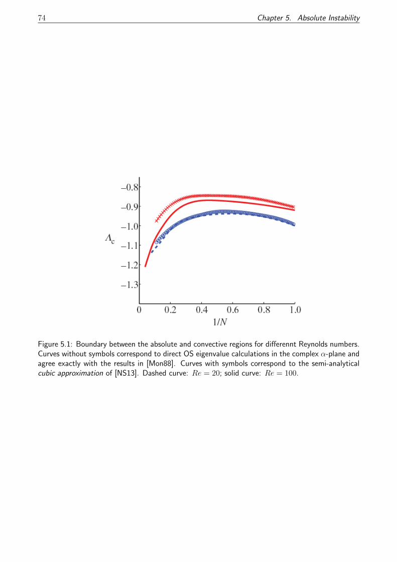
74 Chapter 5. Absolute Instability
Figure 5.1: Boundary between the absolute and convective regions for differennt Reynolds numbers.Curves without symbols correspond to direct OS eigenvalue calculations in the complex α-plane andagree exactly with the results in [Mon88]. Curves with symbols correspond to the semi-analyticalcubic approximation of [NS13]. Dashed curve: Re = 20; solid curve: Re = 100.

Chapter 6
Transient Growth
Overview
We have already seen that plane Couette flow is linearly stable at all finite Reynolds numbers, while
plane Poiseuille flow is stable below a critical Reynolds number Re ≈ 5772. However, it is well
known that such linearly stable flows undergo a transition to a complicated chaotic time-dependent
state (turbulence) below the threshold for the onset of linear instability. This is called the subcritical
transition to turbulence. Below we introduce a toy model to explain this phenomenon and then
connect the toy model back to the Orr–Sommerfeld equation.
6.1 The basic idea
Historically, the linear stability of a system of evolutionary equations was tackled via eigenvalue
analysis. Consider a generic evolutionary system ∂tu = F (u;µ), where u(t) is a trajectory in Cn
and µ is a real parameter. A base state u0 of the system is a solution of the equation F (u0;µ) = 0.
The linearization around the base state refers to the following equation: ∂tu = Ju, where J is the
Jacobian matrix, with Jij = (∂Fi/∂uj)(u0,µ). Let λ1, · · · , λn = spec(J), and let λ0 denote the
eigenvalue with largest real part. The full system is said to be linearly stable if <(λ0) < 0. Suppose
for a critical parameter value µ = µc we have <(λ0) < 0 for µ < µc and <(λ0) > 0 for µ > µc.
Then the system undergoes a bifurcation from linearly stable to linearly unstable at the critical value
µ = µc. The same analysis can usually be applied to spatially extended systems by projecting the
evolutionary equation on to a set of basis functions of dimension n and taking n → ∞, assuming
that the weak solutions so constructed tend to a strong solution.
Such systems can exhibit transient growth in a subcritical parameter regime whereby for suitable
initial conditions involving a superposition of eigenmodes, the L2 norm (or some other more ap-
75
76 Chapter 6. Transient Growth
propriate measure of the energy) of the solution grows initially before eventually decaying at a rate
dictated by λ0. This can happen in two ways. If the eigenvectors do not form a complete set
spanning Cn, then the solution to the initial-value problem will involve contributions such as tpeλjt,
where p ≥ 1 and j ∈ 1, · · · , n, such that transient algebraic growth is possible before the onset
of the asymptotic decay of the solution. We do not consider this case further here (but see Refer-
ence [SH01]). Instead, we consider situations where the eigenvectors of J do indeed span Cn but are
non-orthogonal, corresponding to a situation where J is not a normal operator. In such a scenario,
the L2 norm of solutions involving certain combinations of eigenvectors can grow transiently before
eventually decaying, with transient growth factors ‖u(t)‖2/‖u(t = 0)‖2 that can be as high as
O(105) (e.g. Reference [CC97]). This is the phenomenon of transient growth.
6.2 The toy model
In this section a two-level system is introduced that exhibits the twin effects of non-normality and
nonlinearity. The aim is to start with a set of linear equations and to quantify the influence of the
non-normality on the transient growth at subcritical parameter regimes. Next, a cubic nonlinearity
is introduced and an exact solution for the global mode (and its stability) is obtained. The section
concludes with a crucial discussion about the physical relevance of the system in optics.
6.2.1 Non-normal linear model
We consider the following two-level system
i∂u
∂t= Hu+ i (µ0I + G)u, u ∈ C2, (6.1)
where
H =
(E0 A
A E0
), G =
(−g1 0
0 −g2
),
where E0, A, µ0, g1, g2 are positive real numbers, and where H and µ0I+G are Hermitian matrices,
with [H,G] 6= 0, where [·, ·] denotes the matrix commutator. Note that [H,G] 6= 0 implies that the
operator on the right-hand side of Equation (6.1) is non-normal. One writes down the trial solution
u(t) = u0e−iωt to obtain the following eigenvalues:
ωr = E0± 12
√4A2 − (g1 − g2)2, ωi = µ0− 1
2(g1+g2), 4A2 > (g1−g2)2, Case 1, (6.2)
and
ωr = E0, ωi = µ0− 12(g1+g2)± 1
2
√(g1 − g2)2 − 4A2, 4A2 < (g1−g2)2, Case 2, (6.3)

6.2. The toy model 77
The corresponding eigenvectors for both Case 1 and Case 2 are
u0+ =
(e−iϕ/2
eiϕ/2
), u0− =
(−eiϕ/2
e−iϕ/2
), ϕ = sin−1
(g1 − g2
2A
).
For Case 1, we have |(g1 − g2)/2A| < 1, hence ϕ ∈ R, while for Case 2, ϕ is complex. For
both cases, the eigenvectors are non-orthogonal; the degree of non-orthogonality is expressed by
the relation 〈u0+, u0−〉 = 2i(g2 − g1)/2A. Here, 〈·, ·〉 denotes the usual scalar product on C2, with
〈u,v〉 = uTv, for all column vectors u,v in C2. Orthogonality of eigenvectors is regained for
g1 = g2; this corresponds precisely to [H,G] = 0 and the normality of the (symmetric) operator
H + iG. The crossover between Cases 1 and 2, where (g1 − g2)2 = 4A2 is referred to as a diabolic
point in the literature concerning non-Hermitian quantum mechanics [Gra09, Rot09]; this point truly
is fiendish, since the eigenvectors degenerate and fail to span C2 in this instance. However, in this
work, consideration is given strictly to Case 2, for reasons given in what follows.
Exercise 6.1
1. Call L = H + (µ0I + G). Compute explicitly [L,L†], where the dagger denotes the
Hermitian conjugate of the matrix. Hence veryify that [L,L†] 6= 0. This is the definition
of a non-normal operator.
2. Drive the eigenvalules and eigenvectors for Case 2.
For all possible parameter values, the intrinsic non-Hermiticity of the operator in Equation (6.1)
implies the following nontrivial evolution equation for the L2 norm of the general solution u(t):
‖u‖22 := 〈u, u〉, 1
2
d
dt‖u‖2
2 = 〈u, (µ0 + G)u〉. (6.4)
The quadratic form on the right-hand side can be evaluated in the eigenbasis of the operator G and
a bound on the growth of the L2 norm is obtained:
12
d
dt‖u‖2
2 ≤ [µ0 −min(g1, g2)] ‖u‖22. (6.5)
In this work, we focus on models that exhibit transient growth. Since this relies on the ‘mixing’ of
eigenstates with eigenfrequencies whose imaginary parts are distinct, we are forced by this constraint
to work in Case 2 (this rules out of consideration the diabolic point). With reference to this case,

78 Chapter 6. Transient Growth
and to Equation (6.3), transient non-asymptotic growth is possible in the paramter range
min(g1, g2) < µ0 <12(g1 + g2)−
√(g1 − g2)2 − 4A2. (6.6)
This is the ‘sweet’ operational range where the system is subcritical, in the sense that ωi < 0 for
both eigenvalues, but where the balance between forcing and dissipation is ambiguous, so that the
sign of the upper bound of the growth rate in Equation (6.5) is not definite.
6.2.2 Introduction of nonlinear terms
We add non-linearity to the problem by modifying Equation (6.1) as follows:
i∂u
∂t= Hu+ i (µ0I + G)u+ a
(|u1|2 0
0 |u2|2
)u, (6.7)
where a is real. The evolution of the L2 norm ‖u‖22 is again unchanged under the addition of the
nonlinear term: the quantity ‖u‖22 still evolves according to the norm-evolution first written down for
the linear problem (i.e. Equation (6.4)). However, in contrast to the linear model, Equation (6.7)
has a nonlinear periodic solution, which we find by making the trial solution
u = Re−iΩtu0, ‖u0‖22 = 1, Ω ∈ R. (6.8)
Substitution of Equation (6.8) into Equation (6.7) yields the following eigenvalue problem for u0:
Ωu0 = Lu0 + aR2
(|u01|2 0
0 |u02|2
)u0, L = H + i (µ0I + G) . (6.9)
In general, Equation (6.9) has a family of solutions labelled by the continuous parameter R, with
corresponding eigenvalues Ω(R). However, there is a finite number of R-values consistent with
the requirement =[Ω(R)] = 0; all other R-values correspond to eigensolutions of Equation (6.9)
that are nonetheless inconsistent with Equation (6.8). It is as if we are solving a nonlinear double
eigenvalue problem in the parameters Ω and R (the analogous double eigenvalue problem of linear
algebra is addressed elsewhere [BC78]). Solutions of this double eigenvalue problem are called self-
consistent in the remainder of this work, and can be found analytically for the simple two-level
system considered in this section. Indeed, we have the following theorem:
Theorem 6.1 Let g2 < µ0 < g1, and let
X2 = −(µ0 − g1)(µ0 − g2)
A2. (6.10a)

6.2. The toy model 79
Assume that X2 < 1. Then Equation (6.9) has the following self-consistent solution:
Ω = E0 + aR2, R2 =g1 − g2
a
√1
X2− 1, u0 =
(reiϕ
x
), (6.10b)
where
r =
√µ0 − g2
g1 − g2
, x =
√g1 − µ0
g1 − g2
, ϕ = − sin−1(X). (6.10c)
Proof The so-called self-consistent nonlinear eigenvalue problem refers to the solution u0 of Equa-
tion (6.9) with the constraint that
〈u0, (µ0 + G)u0〉 = 0. (6.11)
To obtain such a solution, we take
u0 =
(reiϕ(R)
x
), r, ϕ, x ∈ R, r2 + x2 = 1; (6.12)
this amounts to a fixed choice for the (arbitrary) global phase of u0. Substitution into Equation (6.11)
yields
r2 (µ0 − g1) + x2 (µ0 − g2) = 0, r2 + x2 = 1, (6.13)
hence
r =
√µ0 − g2
g1 − g2
, x =
√g1 − µ0
g1 − g2
, (6.14)
where r and x are both real because g2 < µ0 < g1. The phase ϕ is not determined by this analysis;
this is obtained by consideration of the full nonlinear eigenvalue problem, which is written out in full
as follows:
Ωreiϕ = L11reiϕ + L12x+ aR2r3eiϕ, (6.15a)
Ωx = L21reiϕ + L22x+ aR2x3. (6.15b)
The imaginary part of the second equation is set to zero to yield a root-finding condition for ϕ:
L(r)21 sinϕ+ L(i)
21 cosϕ+ L(i)22 (x/r) = 0. (6.16)
Because the operator L is symmetric, setting the imaginary part of the first equation to zero yields
precisely the same condition for ϕ. Equation (6.16) simplifies drastically, once the coefficients L(r)21
80 Chapter 6. Transient Growth
etc. are filled in:
A sinϕ+ (µ0 − g2)(x/r) = 0.
Using Equations (6.13)–(6.14), this expression can be written as an explicit function of the problem
parameters alone:
A sinϕ± (µ0 − g2)
√−µ0 − g1
µ0 − g2
= 0,
where the two branches come from taking x = ±√
1− r2 in Equation (6.14), and where the radicand
is positive because of the constraints on the parameters in Theorem 6.1. Hence,
ϕ = ∓ sin−1
(√−(µ0 − g1)(µ0 − g2)
A2
)= ∓ sin−1(X), (6.17)
with ϕ ∈ [−π/2, π/2]. Upon satisfaction of the condition (6.17), Equations (6.15a) and (6.15b) are
consistent, but only in the sense that both equations now imply that Ω is real. The equations (6.15a)
and (6.15b) are made totally consistent by choosing a value of R such that the value of Ω in both
these equations is the same. In terms of the explicit values of the L-matrix, we have
Ω = E0 + A cosϕ(x/r) + aR2r2,
= E0 + A cosϕ(r/x) + aR2x2.
This is a simple quadratic equation in R, for which R has a single real positive root:
R2 =g1 − g2
a
√1
X2− 1.
This procedure therefore picks out two isolated pairs (∓ϕ,R) that leads to a self-consistent solution
of the nonlinear double eigenvalue problem.
Further analytical progress is possible with respect to Equation (6.9): the family of complex-valued
eigenvalues Ω(R) can be controlled in the following manner:
Theorem 6.2 Take as given the non-linear eigenvalue problem (6.9), with eigenvalues Ω(R) ∈ Cfor R ≥ 0. Then
(µ0 − g2)− (g1 + g2) ≤ =(Ω) ≤ µ0 − g2.
Proof Take re−iϕ [Eq. (6.15a)] + x [Eq. (6.15b)] to obtain
Ω = E0 + 2Arx cosϕ+ aR2(r4 + x4) + i(µ0 − g1r2 − g2x
2).
Since x2 + r2 = 1, we have
=(Ω) = (µ0 − g2)− (g1 + g2)r2,
6.2. The toy model 81
with 0 ≤ r2 ≤ 1, hence (µ0 − g2)− (g1 + g2) ≤ =(Ω) ≤ µ0 − g2.
Thus, the range of allowed values of =(Ω) is bounded above and below. In order for =(Ω) = 0 to be
achievable, the upper bound must be non-negative, so that a necessary condition for the existence
of a global mode is µ0 > g2. By Equation (6.5), this is the same necessary condition as the one
required for linear transient growth to occur.
6.2.3 Stability of nonlinear oscillatory state
The stability of the self-consistent oscillatory state is investigated by consideration of a trial solution
u = Re−iΩtu0 + δu,
where R = Rc, and where u0 is the solution of the nonlinear eigenvalue problem. Linearization
around the periodic state yields the following ODE:
id
dtδu = Lδu+ 2R2a
(|u01|2 0
0 |u02|2
)δu+R2e−2iΩt
(u2
01 0
0 u202
)δu,
:= A δu+ e−2iΩtB δu. (6.18)
The manifestly time-dependent term is removed by making the trial solution δu = δve−iΩt, such
that Equation (6.18) becomes
id
dtδv = (A− Ω) δv + Bδv. (6.19)
Equation (6.19) can be further simplified by breaking it up into real and imaginary parts. We take
δv = (a+ ib, u+ iv)T , where a, b, u, and v are real-valued functions of t. We also take B = β+ iγ,
where β and γ are real matrices. Similarly, we write <(A − Ω) := H. Finally, we note that
=(A− Ω) = µ0I + G. Using this notation, we obtain the following real system of equations:
d
dt
a
b
u
v
=
µ0 − g1 + γ11 H11 − β11 0 A
−H11 − β11 µ0 − g1 − γ11 −A 0
0 A µ0 − g2 + γ22 H22 − β22
−A 0 −H22 − β22 µ0 − g2 − γ22
a
b
u
v
. (6.20)

82 Chapter 6. Transient Growth
The results of Theorem 6.1 are now used to fill out the entries in the matrix in Equation (6.20) with
closed-form expressions involving the model parameters:
d
dt
a
b
u
v
=
µ0 − g1 aR2(2r2 − 1) 0 A
+aR2r2 sin 2ϕ −aR2r2 cos 2ϕ
−aR2(2r2 − 1) µ0 − g1 −A 0
−aR2r2 cos 2ϕ −aR2r2 sin 2ϕ
0 A µ0 − g2 −aR2(2r2 − 1)
−aR2(1− r2)
−A 0 aR2(2r2 − 1) µ0 − g2
−aR2(1− r2)
a
b
u
v
(6.21)
Based on this expression of the stability equations, we prove the following theorem:
Theorem 6.3 The oscillatory state in Equation (6.10) is asymptotically unstable.
Proof We write (a, b, u, v)T = eσt(a0, b0, u0, v0), and search for eigensolutions where a0, b0, u0 and
v0 are real. Calling the matrix in Equation (6.21) M, it can be shown by direct computation
that det(M) = 0 identically (e.g. using a symbolic algebra package), such that the characteristic
equation of the matrix M is
σ[σ3 − tr(M)σ2 +m1σ +m2
]= 0, (6.22)
where m1 and m2 are real constants that depend on the problem parameters. A further direct
computation yields
m2 = 8A2(1−X2)[µ0 − 1
2(g1 + g2)
]. (6.23)
Under the twin assumptions that we are in the operating range given by Equation (6.6) and that
0 < X2 < 1, we have that m2 < 0, such that the cubic polynomial in the square brackets
[· · · ] in Equation (6.22) has at least one real positive root, with a corresponding real eigenvector
(a0, b0, u0, v0)T . The corresponding real eigenvalue therefore has σ > 0, hence the system (6.21) is
asymptotically unstable.
6.3 Illustrative numerical examples
It is of interest to examine whether the periodic unstable state has any bearing on the dynamics of
Equation (6.7). Thus, temporal numerical simulations of the same equation are performed. We use

6.3. Illustrative numerical examples 83
the parameter values
E0 = 1, A = 0.1, g2 = 0.01, g1 = g2 + (4A2 + 0.012)1/2, a = 1,
µ0 = 0.95
[12
(g1 + g2)−√
(g1 − g2)2 − 4A2
]. (6.24)
Also, the initial condition was taken to be (A0/√
2)(i, 1)T , where A0 is taken to be small in an ap-
propriate sense, so that the early-stage dynamics correspond to linear theory. The parameters (6.24)
correspond to a subcritical case: both eigenfrequencies of the linearized dynamics possess negative
imaginary parts. However, the same parameters are appropriate for (linear) transient growth, as
outlined in Equation (6.6).
The results are shown in Figure 6.1. The numerical solutions are obtained using an eight-order accu-
rate Runge–Kutta scheme [Gov]. Solutions under the linearized dynamics are shown in Figure 6.1(a).
(a) (b)
Figure 6.1: Solutions of (a) the non-Hermitian linear Schrodinger equation; (b) the non-Hermitiannonlinear Schrodinger equation. The initial data are the parameters are the same in (a) and (b).
Significant transient growth occurs for the initial data and parameter values in Equation (6.24), in
spite of the negatativity of the linear growth rates, i.e. = [spec (L)] ≤ 0: the maximum amplifi-
cation is over 500% in the figure. In contrast, solutions under the nonlinear dynamcis are shown
in Figure 6.1(b). The linear transient growth operates in the same manner as in Figure 6.1, up to
t ≈ 80. Thereafter, a range of possibilities exists, depending on the initial amplitude of the distur-
bance. First, one notes that there is a critical initial amplitude A0c such that limt→∞ ‖u‖2 = Rc;
this is precisely the critical radius for which the nonlinear oscillatory state exists, as in the analysis in
Equation (6.9). Also, for initial amplitudes above this threshold, the same nonlinear oscillatory state
is excited, but is subsequently destabilized, and indefinite exponential growth takes place. Finally,
for initial amplitudes below the same threshold, the nonlinear oscillatory state cannot be maintained,
and the linear dissipation eventually causes the disturbance to decay to zero. For the case A0 > A0c,

84 Chapter 6. Transient Growth
one obtains the eery result that the disturbance grows exponentially fast, in spite of the fact that
the eigenfrequencies of the linearized problem possess negative imaginary parts. This is a subcritical
transition to (nonlinear) instability.
These results point to the following conclusion: linear transient growth by itself is not sufficient
to induce a transition from a regime of small-amplitude disturbances to one of nonlinear instability
in the model equation (6.7). Rather, the transient growth must have available an excitable non-
linear eigenmode, and moreover, the operating parameter regime must be such that the nonlinear
eigenmode is linearly (asymptotically) unstable or neutral. These findings are consistent with the
literature on a vastly more complicated system, namely the subcritical transition to turbulence in
parallel shear flows [SH01, Gro00], where a combination of transient growth and the secondary
instability of coherent states [Wal95, Wal98] is required for subcritical transition to turbulence.
Exercise 6.2
1. The maximum transient growth rate is defined as
γ(t) = supu6=0
‖eLtu‖‖u‖
, (6.25)
where the L2 norm is taken. Show that at each time t the disturbance u that realises the
maximum in Equation (6.25) is the solution of the eigenvalue problem
eL†teLtut = λut, (6.26)
where the subscript t indicates that ut is the disturbance that maximizes the growth rate
γ(t) at the particular time t. The quantity ut is called the optimal disturbance at time
t.
2. Use the parameters (6.24) and the solution (6.26) to generate numerically the curve γ(t),
with 0 < t < 300, say.
3. Download the “.m” code from the website. Run the linear and noninear version of the
code with the initial condition u(t = 0) = u50 (say). Plot the L2 norm of the solution
versus t and compare with Figure 6.1.

6.4. Interlude: Three-dimensional disturbances in plane parallel flows and Squire’s Theorem 85
6.4 Interlude: Three-dimensional disturbances in plane par-
allel flows and Squire’s Theorem
Before applying the theory of transient growth to plane parallel flows, we must first all make a
digression and consider in more detail the notion of three-dimensional disturbances to a plane
parallel flow U0(z), with u = U0(z)x + δu, where δu = (δu, δv, δw), such that the perturbed
velocity u has three non-trivial components. The reason for this is that we will find out that the
optimal disturbance is three-dimensional.
As before, the basic non-dimensional equation of motion is
∂
∂tδu+ U0
∂
∂xδu+ xδw
dU0
dz= −∇p+Re−1∇2δu,
where δp is the perturbation pressure. We operate on both sides with the curl to obtain the linearized
vorticity equation:
∂
∂tδω + U0
∂
∂xδω − U ′0 (x∂xδv − y∂xδu) + U ′0 (y∂zδw + z∂yδw) + yU ′′0 δw = Re−1∇2ω
Call η = z · δ~ω. Clearly,∂η
∂t+ U0
∂η
∂x+ U ′0∂yδw = Re−1∇2η. (6.27)
Next, consider δωx = x · δω and δωy = y · δω. We have
∂
∂tδωx + U0
∂
∂xδωx − U ′0
∂
∂xδv = = Re−1∇2δωx, (6.28a)
∂
∂tδωy + U0
∂
∂xδωy + U ′0
∂
∂xδu+ U ′0
∂
∂zδw + U ′′0 δw = Re−1∇2δωy, (6.28b)
We go over to a normal-mode decomposition with δω ∝ eiαx+iβy, such that ∂x = iα and ∂y = iβ.
Thus, the two vorticity components δωx and δωy become
δωx = ∂yδw − ∂zδv = iβδw − ∂zδv,
δωy = ∂zδu− ∂xδw = −iαδw + ∂zδu.
Put these into Equation (6.28):
∂
∂t(iβδw − ∂zδv) + U0iα (iβδw − ∂zδv)− U ′0iαδv = Re−1∇2 (iβδw − ∂zδv) , (6.29a)

86 Chapter 6. Transient Growth
∂
∂t(−iαδw + ∂zδu) + U0iα (−iαδw + ∂zδu)
+ U ′0iαδu+ U ′0∂zδw + U ′′0 δwRe−1∇2 (−iαδw + ∂zδu) , (6.29b)
Take iβ(6.29a):
∂
∂t
(−β2δw − iβ∂zδv
)+ iαU0
(−β2δw − iβ∂zδv
)− iαU ′0 (iβδv) = Re−1∇2
(−β2δw − iβ∂zδv
). (6.30a)
Also, take iα(6.29b):
∂
∂t
(α2δw + iα∂zδu
)+ iαU0
(α2δw + iα∂zδu
)+ iαU ′0 (iαδu) + iαU ′0∂zδv + iαU ′′0 δw = Re−1∇2
(α2δw + iα∂zδu
). (6.30b)
Subtract:
∂
∂t
(−β2δw − α2δw − iβ∂zδv − iα∂zδu
)+ iαU0
(−β2δw − α2δw − iβ∂zδv − iα∂zδu
)+ iαU ′0 (−iβδv − iαδu− ∂zδv)− iαU ′′0 δw = Re−1∇2
(−β2δw − α2δw − iβ∂zδv − iα∂zδu
)Use incompressibility:
iαδu+ iβδv + ∂zδw = 0
hence
∂2zδw − iαδu− iβδv,
and thus∂
∂t∇2δw + iαU0∇2δw − iαU ′′0 δw = ∇4δw.
Going over to the normal-mode decomposition, this is
∂
∂t
(∂2z − k2
)δw + iαU0
(∂2z − k2
)δw − iαU ′′0 δw =
(∂2z − k2
)2δw, k2 = α2 + β2.
With δw ∝ e−iαct this is
iα (U0 − c)(∂2z − k2
)δw − iαU ′′0 δw = Re−1
(∂2z − k2
)2δw, (6.31a)
which is precisely the Orr–Sommerfeld equation. However, we have a further equation for the
wall-normal vorticty (Equation (6.27)) which now reads
iα(U0 − c)η + iβU ′0δw = Re−1(∂2z − k2)η. (6.31b)
6.4. Interlude: Three-dimensional disturbances in plane parallel flows and Squire’s Theorem 87
Equations (6.31) are the Orr–Sommerfeld–Squire equations.
Equation (6.31a) can be mapped into a two-dimensional Orr–Sommerfeld equation by the introduc-
tion of the variables
α2D = k =√α2 + β2, (6.32a)
Re2D =α
α2D
Re =
√α2
α2 + β2Re. (6.32b)
Thus, Equation (6.31a) can be rewritten as
iα2D (U0 − c)(∂2z − α2
2D
)δw − iαU ′′0 δw = Re−1
2D
(∂2z − α2D
)2δw,
which is precisely the Orr–Sommerfeld equation in two dimensions. From Equation (6.32) we have
Re2D < Re.
Thus, we have shown the following result:
Lemma 6.1 To each three-dimensional Orr–Sommerfeld–Squire mode there corresponds a two-
dimensional Orr–Sommerfeld mode at a lower Reynolds number.
This enables us to prove Squire’s theorem:
Theorem 6.4 Given ReL as the critical Reynolds number for the onset of linear instability for
a given (α, β), the Reynolds number Rec below which no exponential instabilities exist for any
wavenumbers satisfies
Rec := minα,β
ReL(α, β) = minαReL(α, 0).
Thus, parallel shear flows fisrt become unstable to two-dimensional wavelike perturbations at a
value of the Reynolds number that is smaller than any value for which unstable three-dimensional
perturbations exist. That is the reason why no generality was lost to date in studying only the
two-dimensional disturbances for the plane parallel flows.
The proof of Squire’s theorem follows directly from the Squire transformation (6.32): if a three-
dimensional mode is unstable, then a two-dimensional mode is unstable at a lower Reynolds number.
We also have the following result for so-called pure Squire modes (A solution of the Orr–Sommerfeld–
Squire equations with w = 0 is called a pure Squire mode):
Theorem 6.5 The eigenvalues of all pure squire modes are damped, i.e. ci < 0 for all α, β and
Re, for all pure Squire modes

88 Chapter 6. Transient Growth
The proof here is straightforward: we take w = 0 in the Squire equation (6.31b). We then multiply
by η∗ and integrate from z = 0 to z = 1:
λ
∫ 1
0
|η|2 dz + iα
∫ 1
0
U0|η|2 = Re−1
∫ 1
0
η∗(∂2z − k2
)η, λ = −iαc. (6.33)
Since η = z ·δω = iαδv− iβδu we have η = 0 at z = 0, z = 1. This enables us to do integration by
parts on the right-hand side of Equation (6.33) and to set the boundary terms to zero. We obtain
λ
∫ 1
0
|η|2 dz + iα
∫ 1
0
U0|η|2 = −Re−1
∫ 1
0
(|∂zη|2 + k2|η|2
)dz.
Taking real parts, we have
λr‖η‖22 = −Re−1
(‖∂zη|22 + k2‖η‖2
2
)hence λr‖η‖2
2 < 0, hence ci < 0 as required.
Transient behaviour
It is tempting to ask why wave introduced the Orr–Sommerfeld Squire equations when the end
result has been a theorem showing that as far as eigenvalues are concerned, the three-dimensional
disturbances are not important. The answer is that stability theory is about more than eigenvalues.
Eigenvalue analysis is only valid as t → ∞. For finite times, we must consider the full initial value
problem. The initial value problem for the Squire equation reads
∂η
∂t+ iαU0(z)η + iβU ′0δw = Re−1
(∂2z − k2
)η.
For α = 0 this reads∂η
∂t+α2
Reη =
1
Re∂2zη + iβU ′0δw. (6.34)
Let us further focus on the large-Reynolds number flows, and focus on the case where we can take
Re→∞, such that Equation (6.34) reads
∂η
∂t= −iβU ′0δw.
This is a first-order separable ODE, with solution
η(z, t) = η(z, 0)− iβU ′0(z)
∫ t
0
δw(z, t) dt.

6.5. Transient growth in plane parallel flows 89
For short times we can take δw(z, t) outside the integrand, leaving
η(z, t) ≈ η(z, 0)− iβU ′0δw(z, 0)t (6.35)
Thus, the vorticity grows linearly with time for short times. This is the notion of a transient
instability. Of course, what happens as t → ∞ is not predicted by Equation (6.35) – that is
determined by the eigenvalue analysis. But it is of interest to study in a systematic way the transient
behavior of the Orr–Sommerfeld–Squire equations at finite times, i.e. before the eigenvalue analysis
becomes the factor determining the time evolution. We do this in the next section.
6.5 Transient growth in plane parallel flows
6.5.1 Formulation
The Orr–Sommerfeld–Squire equation for a generic problem in the hydrodynamic stability of a
parallel flow can be written down in generic form as follows:
Lχ = λMχ, (6.36)
The stability problem is solved at a particular set of wavenumbers (α, β), and the Orr–Sommerfeld–
Squire matrices L and M and the eigenvalue λ all depend on the wavenumbers. Recall, the
state vector χ is obtained by writing the wall-normal velocity and vorticity in a finite Chebyshev
approximation:
w(z) =N∑i=0
AiTi(x), η =N∑i=0
BiTi(x), x = 2z − 1,
such that
χ = (A0, · · · , An, B0, · · · , Bn)T .
Now, it can be shown that the matrices in Equation (6.36) can be used to solve the corresponding
initial-value problem (e.g. Reference [ONSS13]). The initial-value problem is formulated as follows:
∂
∂tMχ = Lχ, t > 0, (6.37a)
with initial condition
χ(t = 0) = χ0, χ0 = (x0, · · · , xn, y0, · · · , yn)T , (6.37b)

90 Chapter 6. Transient Growth
and where
x0 =1
π
∫ 1
−1
T0(x)w(
12(x+ 1), t = 0
) dx√1− x2
, (6.38a)
xi =2
π
∫ 1
−1
Ti(x)w(
12(x+ 1), t = 0
) dx√1− x2
, i 6= 0, (6.38b)
y0 =1
π
∫ 1
−1
T0(x)η(
12(x+ 1), t = 0
) dx√1− x2
, (6.38c)
yi =2
π
∫ 1
−1
Ti(x)η(
12(x+ 1), t = 0
) dx√1− x2
, i 6= 0. (6.38d)
It can be easily seen that the solution to Equation (6.37) can be written as
χ(tn) = X (tn)χ0, tn = n∆t, n = 0, 1, · · · ,
where ∆t→ 0, keeping tn = t finite. Also,
X (t) = lim∆t→0
[(M−∆tL)−1M
]n. (6.39)
Note that Equation (6.39) amounts to solving the linear differential algebraic equation (DAE) (6.37a)
using the backward Euler method.
6.5.2 The method
The idea of the transient-growth calculation is to start with the energy norm
E(t) =
∫ 1
0
(|∂zw|2 + k2|w|2 + |η|2
)dz, k2 = α2 + β2, (6.40)
and at each point in time to optimize the energy norm subject to the constraint that E(0) = 1.
The resulting maximum energy is called the transient growth rate, G(t). These calculations can be
done within the framework of Section 6.5.1 as follows. First, the energy norm in Equation (6.40) is
identified with a scalar product on the space of admissible χ-vectors:
E(t) = 12
∫ 1
−1
dx
∣∣∣∣∣N∑i=0
AiexT′i (x)
∣∣∣∣∣2
+ k2
∣∣∣∣∣N∑i=0
AiTi(x)
∣∣∣∣∣2
+
∣∣∣∣∣N∑i=0
BiTi(x)
∣∣∣∣∣2 , ex =
dx
dz= 2,
=∑i,j
A∗iAj
(12e2x
∫ 1
−1
T ′i (x)T ′j(x)dx
)+∑i,j
A∗iAj
(12k2
∫ 1
−1
Ti(x)Tj(x)dx
)+∑i,j
B∗iBj
(12
∫ 1
−1
Ti(x)Tj(x)dx
).
6.5. Transient growth in plane parallel flows 91
Call
T(1)ij = 1
2e2x
∫ 1
−1
T ′i (x)T ′j(x)dx,
T(0)ij = 1
2
∫ 1
−1
Ti(x)Tj(x)dx.
We have
E(t) =∑i,j
A∗iAjT(1)ij + k2
∑i,j
A∗iAjT(0)ij +
∑i,j
B∗iBjT(0)ij ,
=
⟨χ,
(T(1) + k2T(0) 0
0 T(0)
)χ
⟩,
:= 〈χ,Gχ〉.
Here, the brackets denote the usual scalar product on the space of χ-vectors, and the matrix G is
symmetric positive-definite. Thus, the equation
E(t) = 〈χ,Gχ〉
defines a scalar product on the space of χ-vectors. However, we have
χ = X (t)χ0,
hence
E(t) = 〈χ0,X (t)†GX (t)χ0〉.
Thus, the optimization to be performed can be recast as an optimization of the functional
E[χ0] = 〈χ0,X (t)†GX (t)χ0〉,
subject to the constraint that
〈χ0,Gχ0〉 = 1.
In other words, we have the following Lagrange-multiplier problem:
E[χ0] = 〈χ0,X (t)†GX (t)χ0〉 − λ (〈χ0,Gχ0〉 − 1) .
The optimum vector is obtained by setting
δE
δχ∗= 0,
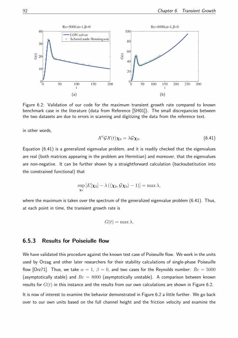
92 Chapter 6. Transient Growth
(a) (b)
Figure 6.2: Validation of our code for the maximum transient growth rate compared to knownbenchmark case in the literature (data from Reference [SH01]). The small discrepancies betweenthe two datasets are due to errors in scanning and digitizing the data from the reference text.
in other words,
X †GX (t)χ0 = λGχ0. (6.41)
Equation (6.41) is a generalized eigenvalue problem, and it is readily checked that the eigenvalues
are real (both matrices appearing in the problem are Hermitian) and moreover, that the eigenvalues
are non-negative. It can be further shown by a straightforward calculation (backsubstitution into
the constrained functional) that
supχ0
[E[χ0]− λ (〈χ0,Gχ0〉 − 1)] = maxλ,
where the maximum is taken over the spectrum of the generalized eigenvalue problem (6.41). Thus,
at each point in time, the transient growth rate is
G(t) = maxλ.
6.5.3 Results for Poiseiulle flow
We have validated this procedure against the known test case of Poiseuille flow. We work in the units
used by Orzag and other later researchers for their stability calculations of single-phase Poiseuille
flow [Orz71]. Thus, we take α = 1, β = 0, and two cases for the Reynolds number: Re = 5000
(asymptotically stable) and Re = 8000 (asymptotically unstable). A comparison between known
results for G(t) in this instance and the results from our own calculations are shown in Figure 6.2.
It is now of interest to examine the behavior demonstrated in Figure 6.2 a little further. We go back
over to our own units based on the full channel height and the friction velocity and examine the

6.5. Transient growth in plane parallel flows 93
(a) t = 0.05 (b) t = 0.1 (c) t = 0.15
(d) t = 0.5 (e) t = 1 (f) t = 2
(g) t = 5 (h) t = 10
Figure 6.3: Time evolution of the optimal transient growth rate as a function of the wavenumbersα (streamwise) and β (spanwise). Between t = 0.1 and t = 10 the optimal disturbance moves frombeing spanwise-dominated to streamwise-dominated.
features of the transient growth in the supercritical case Re = 8000, Re∗ =√
8× 8000 ≈ 252.9822,
for various times t ∈ [0, 2] (corresponding to times [0, 2]Re∗/2 in Figure 6.2). The resulting study
is presented in Figure 6.3 where it should be noticed that it is the square root of the energy of the
most-amplified disturbance that is plotted in a wavenumber space, for different t-values. For very
short times (t = 0.1) the transiently most-amplified mode has a wavevector with components in
both the streamwise and spanwise directions (at t = 0.1, maxα,β Gα,β(t) occurs at (α, β) ≈ (3, 8)).
As time goes by, the most-amplified mode moves to a more spanwise wavenumber such that by
t = 1 the maximum value maxα,β Gα,β(t) occurs at α ≈ 0 and β = 6. Thereafter, there is a slow
evolution of the trajectory of the most-amplified disturbance through the wavenumber space away
from spanwise wavenumbers towards streamwise ones (the eigenvalue theory predicts that as t→∞

94 Chapter 6. Transient Growth
Figure 6.4: Eigenvalue of most-dangerous mode of the Orr–Sommerfeld–Squire equations, withRe = 5000. The most-dangerous mode according to eigenvalue analysis (valid as t → ∞) is astreamwise one.
the most-amplified disturbance is a streamwise-only mode – Figure 6.4). By t = 10 the asymptotic
state is reached and the most-amplified disturbance is indeed streamwise-only.

Chapter 7
Weakly nonlinear theory
7.1 Overview
Beyond linear theory, analytical progress can be made in certain scenarios wherein a separation of
scales occurs. The idea here is to break up the eigenmodes of the linear theory into two sets. In
the first set, the growth rates of the linear theory are O(1), while in the second set, the normal
modes possess large damping rates of magnitude 1/ε, so that a separation of timescales between
the two sets occurs. Thus, two sets emerge, corresponding to fast dynamics and slow dynamics.
The modes belonging to the fast set can be viewed as slaved to the slow modes, and do not evolve
dynamically. Analytical expressions for the fast modes in terms of the slow modes can be derived,
which in turn are substituted back into the equations for the slow modes, leading to a simplified
system of differential equations for the fast modes.
7.2 Example – Cahn–Hilliard equation
We will start with an example of a nonlinear equation amenable to a weakly nonlinear analysis.
The direct relevance to Fluid Dynamics here is not immediately obvious, but it serves here as an
excellent example of the methodology. We therefore study the following Cahn–Hilliard equation
in one spatial dimension:
∂C
∂t= ∇2
(C3 − C − γ∇2C
), t > 0, x ∈ (0, L), (7.1)
with initial date C(x, t = 0) = Cinit(x) and periodic boundary conditions on the interval (0, L).
Also, D and γ are positive constants.
95
96 Chapter 7. Weakly nonlinear theory
It can be seen that the Cahn–Hilliard equation is mass-conserving,
d
dt
∫ L
0
C(x, t) dx = 0 (7.2)
In this example, we take ∫ L
0
C(x, t) dx = 0,
corresponding to a symmetric mixture. It can also be seen that the state C(x, t) = C0, with
C0 is a solution of the Cahn–Hilliard equation for a symmetric mixture, and that the state is
linearly unstable with respect to small-amplitude perturbations. For, starting with the trial solution
C(x, t) = C0 + εeν+ikx, the growth rate ν satisfies the dispersion relation
ν = Dk2(1− γk2),
with cutoff wavenumber kc = γ1/2 and most-dangerous mode kmax = kc/√
2.
We now explore the weakly nonlinear dynamcis of Equation (7.1). For simplicity, we will examine
a scenario where the set of fast modes comprises a single normal mode, and that all other modes
are damped according to linear theory. This corresponds to a situation just above criticality. The
application of weakly nonlinear theory to this scenario where the set of fast modes contains only one
element is called Stuart–Landau theory. Parameters appropriate for this regime are L = 1 and
γ = 1/8π2. The most-dangerous mode therefore occurs at k1 = 2π and the cutoff is at kc =√
2k1,
with k1 < kc < 2k1, such that precisely one unstable mode fits inside the box.
The complete solution of Eq. (7.1) is expanded as a Fourier series,
C(x, t) =∞∑
n=−∞
An(t)eiknx, kn = (2π/L)n, A−n = A∗n, (7.3)
with A0 = 0 for symmetric mixtures. The solution (7.3) is substituted into Equation (7.1). One
obtains the following amplitude equations:
dAndt
= ν(kn)An −Dk2n
∞∑p=−∞
∞∑q=−∞
ApAqAn−p−q. (7.4)
Equation (9.5) is an example of a nonlinearity by way of a four-wave interaction. Four-wave
interactions are the hallmark of a cubic nonlinearity. Now, for a barely-supercritical system, the
fundamental mode (n = ±1) has a positive linear growth rate, while all other modes have a negative
linear growth rate. Initially therefore, the fundamental dominates the evolution. Overtones will only
be relevant if they couple to the fundamental. We therefore simplify Eq. (9.5) by considering the
dominant modes. These will be the fundamental and a handful of overtones. In fact, we reduce
7.2. Example – Cahn–Hilliard equation 97
the equations down to a triple by considering the fundamental and the n = 2, 3 overtones, and by
neglecting all other modes. A further simplification occurs in the overtone equations, wherein one
considers the most-dominant interaction terms only; i.e. those that involve a power of A1. One
arrives at the following set of equations
dA1
dt= ν(k1)A1 −Dk2
1A1
(6|A2|2 + 6|A3|2 + 3|A1|2
)− 3Dk2
1A3A∗21 , (7.5a)
dA2
dt= ν(k2)A2 − 6Dk2
2|A1|2A2, (7.5b)
dA3
dt= ν(k3)A3 −Dk2
3A31. (7.5c)
Because of the cubic interaction, a strange thing occurs, whereby the right-hand side of the A2
equation is proportional to A2 itself, meaning that the amplitude |A2| can be controlled in the
following manner:12
d
dt|A2|2 =
(ν(k2)− 6Dk2
2|A1|2)|A2|2 ≤ ν(k2)|A2|2,
By Gronwall’s inequality, we have the following further inequality:
|A2(t)| ≤ |A2(0)|eν(k2)t,
which is exponentially decaying because only the fundamental is linearly unstable. Thus, in the set of
modes A1, A2, A3, the mode A2 is decaying. In contrast, the right-hand side of the A3-equation is
not proportional to A3, and the corresponding amplitude is not controlled. Indeed, Equation (7.5b)
is a first-order homogeneous ODE for A2, while the corresponding equation for A3 is first-order and
inhomogeneous, with solution
A3 = A3(0)eν(k3)t −Dk23eν(k3)t
∫ t
0
e−ν(k3)s[A1(s)]3 ds. (7.6)
We now invoke the separation-of-timescales argument, assuming that |ν(k1)/ν(k2)| 1, and
|ν(k1)/ν(k3)| 1, with ν(k1) > 0 and the other two growth rates negative. It is as if we are
taking the limit ν(k2) → −∞ and ν(k3) → −∞. In this limit, the A2 mode is damped rapidly to
zero, so that under separation of scales, we have
A2 = 0.
Consideration is given to Equation (7.6) in the same limit. In this limit, the most-rapidly varying
term in the integral is e−ν(k3)s, compared to which A1(s) varies slowly and can be taken outside the

98 Chapter 7. Weakly nonlinear theory
integral, leaving
A3(t) = A3(0)eν(k3)t −Dk23eν(k3)t
∫ t
0
e−ν(k3)s[A1(s)]3 ds,
≈ A3(0)eν(k3)t −Dk23eν(k3)t[A1(t)]3
∫ t
0
e−ν(k3)s ds,
= A3(0)eν(k3)t +Dk2
3
ν(k2)eν(k3)t[A1(t)]3
(e−ν(k3)t − 1
),
=Dk2
3
ν(k2)[A1(t)]3 +
[A3(0)eν(k3)t − 6Dk2
3
ν(k2)[A1(t)]3eν(k3)t
],
which in the limit of infinite separation of scales reduces to
A3(t) =Dk2
3
ν(k2)[A1(t)]3.
Summarizing, in the limit of infinite separation of scales, we have
A2 = 0, A3(t) =Dk2
3
ν(k2)[A1(t)]3 := CA3
1. (7.7)
These identities are now substituted back into Equation (7.5a) for A1, which now is constituted in
closed form:
dA1
dt= ν(k1)A1 −Dk2
1A1
(3|A1|2 + 6C2|A1|6
)− 3CA1|A1|2,
= ν(k1)A1 −Dk21A1
(3|A1|2 + 3C|A1|4 + 6C2|A1|6
). (7.8)
A solution to the A1-equation is readily available in closed form, and backsubstitution into Equa-
tion (7.7) yields A3. Thus, under the separation-of-scales assumption, A3 does not evolve dynami-
cally – it is slaved to the mode A1. Also, from Equation (7.8), we can see that
12
d
dt|A1|2 = ν(k1)|A1|2 −Dk2
1|A1|2P(|A1|2),
where
P(x2) = 3x2 + 3Cx4 + 6C2x6 ≥ 0
meaning that exponential linear growth term ν(k1)|A1|2 is eventually balanced by the nonlinear term
Dk21|A1|2P(|A1|2) and the nonlinearity in this instance is saturating.
The theory can be extended to involve the five modes A1, A2, A3, A4, A5, leading to the following
7.2. Example – Cahn–Hilliard equation 99
amplitude equations:
dA1
dt= ν(k1)A1 −Dk2
1A1
(3|A1|2 + 6|A2|2 + 6|A3|2 + 6|A4|2 + 6|A5|2
)−3Dk2
1A3(A∗21 + 2A2A∗4 + A3A
∗5)− 6Dk2
1A4(A∗1A∗2 + A2A
∗5)
−3Dk21A5(A∗22 + 2A∗1A
∗3), (7.9)
dA2
dt= ν(k2)A2 − 6Dk2
2|A1|2A2, (7.10)
dA3
dt= ν(k3)A3 −Dk2
3A31, (7.11)
dA4
dt= ν(k4)A4 − 3Dk2
2A21A2, (7.12)
dA5
dt= ν(k5)A5 − 3Dk2
5A21A3, (7.13)
where in the equations for the harmonics we have kept only those interaction terms that involve the
highest powers of A1 and A∗1.
Again, in the limit of infinite separation of scales, we have A2 → 0 and hence by recursion, A4 → 0,
and thus we reduce to a triple of equations for odd modes:
dA1
dt= ν(k1)A1 −Dk2
1A1
(3|A1|2 + 6|A3|2 + 6|A5|2
)−3Dk2
1A3(A∗21 + A3A∗5)− 6Dk2
1A∗1A∗3A5, (7.14)
dA3
dt= ν(k3)A3 −Dk2
3A31, (7.15)
dA5
dt= ν(k5)A5 − 3Dk2
5A21A3. (7.16)
The limit of infinite separation-of-scales is invoked again and we obtain
A3 =Dk2
3
ν(k3)A3
1, A5 =3D2k2
5k23
ν(k3)ν(k5)A5
1. (7.17)
Thus, we have An ∝ An1 , valid clearly (by recursion) for all n ∈ 3, 5, 7, · · · . This is a hallmark of
the Stuart–Landau theory: the amplitude of the harmonics is a power of the amplitude of
the fundamental. The Stuart–Landau law (7.17) is substituted back into Equation (7.14). One
obtainsdA1
dt= ν(k1)A1 −Dk2
1A1Q(|A1|2), (7.18)
where again, Q ≥ 0 and the nonlinearity is saturating.
The theory in Equations (7.17)–(7.18) is now checked against numerical simulation. The numerical
simulation is carried out with the FDCH parallel Cahn–Hilliard solver [NSN15]. The numerical

100 Chapter 7. Weakly nonlinear theory
simulation seeded with the initial condition
Cinit = ε cos(k1x), ε = 10−4. (7.19)
A spectral analysis of the numerical solution was obtained and the results plotted in Fig. 7.1. An
Figure 7.1: (Figure from Reference [NSN15]). Comparison between weakly linear theory and directnumerical simulation. Model parameters: D = 1, L = 1, and γ = 1/8π2. Simulation parameters:∆x = 1/304, ∆t = 10−8. The simulation results are shown in thick lines: solid line: |A1|, dottedline: |A3|, dashed line: |A5|. The predictions from weakly nonlinear theory are shown in thinlines with symbols. Squares and circles: predictions based on Equation (7.17) for |A3| and |A5|respectively. Diamonds: prediction based on Equation (7.18) for |A1|. The main figure is presentedagain in the inset using a log-log scale to show the initial layer of the dynamics before the onset ofslaving.
additional log-log plot shown in the inset of the same figure reveals the presence of odd-numbered
harmonics even at t = 0. This is due to roundoff error in the simulation (the simulations used the
IEEE double precision format). A combination of roundoff error and numerical error also leads to
the the presence of some transient noise in the amplitude |A5|. However, these effects are rapidly
dissipated, such that the eventual outcome of the simulation demonstrates excellent agreement
between the theory based on Equations (7.17)–(7.18) and the FDCH code.

7.3. General theory 101
7.3 General theory
The general theory of slaving involves a set of ODEs,
dx
dt= f(x, y), x ∈ Cn, (7.20a)
dy
dt= −1
εDy + g(x, y), y ∈ Cm, (7.20b)
valid for t > 0, with initial data
x(t = 0) = x0, y(t = 0) = y0. (7.20c)
where D is a diagonal matrix with Dii > 0.
An implicit solution of the y-equation is obtained as follows:
yi(t) = yi(0)e−tDii/ε + e−tDii/ε∫ t
0
e−tDii/εgi(x(s), y(s)) ds
Clearly, yi(t) varies on two timescales: the rapid timescale 1/ε, and the slow timescale which is
O(1), and we write
yi(t) = yi(t, t/ε),
such that
yi(t) = yi(0)e−tDii/ε + e−tDii/ε∫ t
0
etDii/εgi(x(t), y(t, t/ε)) dt
suppressing the difference between the dummy variable of integration and t for the time being. We
make the substitution t = t/ε. Thus,
yi(t) = yi(0)e−tDii/ε + εe−tDii/ε∫ t/ε
0
etDiigi(x(εt), y(εt, t)) dt.
We now solve the integral equation recursively. To lowest order in ε, we have
yi(t) = yi(0)e−tDii/ε + εe−tDii/ε∫ t/ε
0
etDiigi(x(εt), yi(0)e−tDii t) dt.
We take εa < t, where a < 1. Then the first term is bounded by
yi(0)e−Dii/ε1−a → 0, ε→ 0,
such that
yi(t)→ εe−tDii/ε∫ t/ε
0
etDiig(x(εt), 0)dt = e−tDii/ε∫ t
0
etDii/εgi(x(t), 0)dt, ε→ 0,
102 Chapter 7. Weakly nonlinear theory
and provided t < 1/ε the term g(x(t), 0) can be treated as a constant, leaving
yi(t)→ e−tDii/εgi(x(t), 0)
∫ t
0
etDii/εdt ε→ 0,
leaving
yi(t) ∼ε
Dii
gi(x(t), 0), t < 1/ε, ε→ 0,
which is the final result.
7.4 Example – Kuramoto–Sivashinsky equation
Consider the following longwave model for waves on a thin film in the presence of surface tension
and inertia, taken from Reference [BCF95]:
∂h
∂t+
∂
∂x
[c0h+ h2(V + hW ) +Re(R + hT )
∂h
∂x+M
∂2h
∂x2+ReS
We
∂3h
∂x3
]= 0,
x ∈ (0, L), t > 0, (7.21)
with applied periodic boundary conditions in the x direction. Here c0, V,W,Re,R, T,M, S,Weare positive real constants of the model.
Exercise 7.1 Compute the dispersion relation for the linearized equation of motion.
Answer clue:
ν = ik(−c0 +Mk2) +Re k2
(R− S
Wek2
).
Exercise 7.2 Show that the amplitude equation corresponding to Equation (7.21) is
dAndt
= νAn + (iα + nβ)∞∑
p=−∞
pApAn−p + iχ∞∑
p=−∞
∞∑q=−∞
pApAqAn−p−q, (7.22)
where
α = k1V, β = 12k2
1ReT, χ = 34ik1W
and where k1 is the fundamental wavenumber.
Exercise 7.3 Assume that the fundamental is a standing wave, with c0 = Mk21. By keeping only

7.4. Example – Kuramoto–Sivashinsky equation 103
the first three modes, and by taking δ = Mk31, derive the following amplitude equations:
dA1
dt= σ1A1 + (iα + β)A∗1A2 + iχA2
1A∗1, (7.23a)
dA2
dt= (σ2 − 6iδ)A2 + (iα + 2β)A2
1, (7.23b)
dA3
dt= (σ3 − 24iδ)A3 + 3(iα + 3β)A1A2 + iχA3
1, (7.23c)
where σn = <[ν(kn)].
Exercise 7.4 Working near criticality, with σ1 > 0, σn < 0, and |σn| σ1 for n ≥ 2 argue as
before that
An ∝ An1 , n ≥ 2.
Chapter 8
Direct numerical simulation of the
incompressible Navier–Stokes equations
8.1 Overview
In this section we outline a numerical method to solve the incompressible Navier–Stokes equations.
The method will be broken down piece-by-piece and numerical algorithms to solve each piece will
be introduced. Analysing and implementing these algorithms will be the subject of this and future
chapters. The aim is to develop a complete understanding of a parallel DNS solver called TPLS.
8.2 The basic equations
We start with the incompressible Navier–Stokes in non-dimensional form:
∂u
∂t+ u · ∇u = −∇q +
1
Re∇ ·[µ(∇u+∇uT
)]∇ · u = 0, t > 0, (8.1)
with initial conditions
u(x, t = 0) = u0, q(x, t = 0) = q0, ∇ · u0 = 0,
defined on the domain (x, y, z) ∈ [0, Lx] × [0, Ly] × [01]. For definiteness, we work in a channel
geometry, with the following boundary conditions:
u(z = 0) = u(z = 1) = 0,
and with periodic boundary conditions in the other two directions. Ordinarily, the viscosity µ is a
constant; however, it is treated here as a quantity that potentially varies in space and time, meaning
104

8.3. The method 105
that our discussion is quite general, and can be extended to large-eddy simulations and Reynolds-
averaged simulation modelling of turbulence. A schematic of the computational domain is illustrated
Figure 8.1: (Picture thanks to James Fannon) Computational domain Ω = [0, Lx] × [0, Ly] ×[0, Lz = 1]. Periodic boundary conditions are used in the streamwise (faces AB) and spanwise(faces CD) directions, while no-slip boundary conditions are used on faces E and F .
in figure 8.1, where the length scale is normalised with respect to the channel height i.e. Lz = 1.
A driving force is introduced in the streamwise (x-direction), such that
q(x, t) = p(x, t)− |dP/dL|x,
where |dP/dL| is the constant pressure drop. Thus, the equations to be solved now read
∂u
∂t+ u · ∇u = −∇p+
1
Re∇ ·[µ(∇u+∇uT
)]+ x|dP/dL|, ∇ · u = 0, t > 0. (8.2)
It is difficult to evolve these equations forward in time because there is no explicit equation for p.
The solution to this problem is to use a projection method. This will be done in tandem with a
finite-volume discretization.
8.3 The method
We employ a uniform finite-volume discretization. This is similar in spirit to a uniform finite-difference
discretization, except that more attention is paid to the physics of each computational cell. Each
cell is of size ∆x3, but now scalar quantities are defined at cell centres and vector quantities on the
appropriate cell faces. In this way, the divergence of a vector flux is automatically defined at cell
centres and also, is automatically computed by a centred finite difference, which has higher-order
accuracy than a more naive approach, and also takes account of the physics of the fluxes flowing

106 Chapter 8. Direct numerical simulation of the incompressible Navier–Stokes equations
Figure 8.2: Schematic description of a two-dimensionial MAC grid
into and out of each computational cell. A schematic description of this setup is given in Figure 8.2.
This choice of grid is called a marker-and-cell (MAC) grid.
To evolve the equations forward in time, operator-splitting is carried out in two distinct half-steps.
In the first half-step, an intermediate velocity u∗ is computed by momentarily ignoring the pressure
contribution in the momentum equation:
u∗ − un = −u · ∇u+1
Re∇ ·[µ(∇u+∇uT
)].
The precise manner in which u∗ is extracted from this equation is discussed below. We first of all
however describe the second half-step which is got by considering the pressure contribution:
un+1 − u∗
∆t= −∇pn+1 + |dP/dL|x. (8.3)
We take the divergence on both sides and impose the constraint that ∇ · un+1 = 0, leading to
∇pn+1 =∇ · u∗
∆t. (8.4)
By solving the Poisson equation (8.4) the pressure at timestep n + 1 is obtained. This is then
substituted back into Equation (8.3) to give
un+1 = u∗ −∆t∇pn+1 + ∆t|dP/dL|x.
We now describe in detail the implementation of the momentum half-step.

8.4. Discretzation of the momentum half-step in space and time 107
8.4 Discretzation of the momentum half-step in space and
time
Recall, in the momentum half-step, the equation
u∗ − un
∆t+ u · ∇u =
1
Re∇ ·[µ(∇u+∇uT
)](8.5)
is solved for u∗. Here, µ is the (possibly varying) viscosity, defined at cell centres. Below we show
how Equation (8.5) is disctetized in space and time.
Temporal discretization
The viscous term is broken up first of all into contributions that are more convective in nature and
other contributions that can be treated are more of a diffusive character. The more convective parts
are identified as1
Re
∂
∂xi
(µ∂ui∂xj
), j = 1, 2, 3,
while the more diffusive parts are identified as
1
Re
∂
∂xi
(µ∂uj∂xi
):= D (u) , j = 1, 2, 3.
For example, for j = 1 (with u = (u, v, w)), the more convective parts are
1
Re
[∂
∂x
(µ∂u
∂x
)+
∂
∂y
(µ∂v
∂x
)+
∂
∂z
(µ∂w
∂x
)]and the more diffusive parts are
1
Re
[∂
∂x
(µ∂u
∂x
)+
∂
∂y
(µ∂u
∂y
)+
∂
∂z
(µ∂u
∂z
)]:= D1(u).
Thus, Equation (8.5) is rewritten as
u∗ − un
∆t=
[−u · ∇u+
ejRe
∂
∂xi
(µ∂ui∂xj
)]+ D (u) . (8.6)
where ej is a unit vector in the jth Cartesian direction. The terms in the square bracket are now
bundled together as a convective term C and Equation (8.6) is discretized in time using Adams–
Bashforth discretization on convective terms and Crank–Nicholson discretization on the diffusive

108 Chapter 8. Direct numerical simulation of the incompressible Navier–Stokes equations
contribution, giving
u∗ = un + ∆t(Cn − 4
3Cn−1 + 5
12Cn−2
)+ 1
2∆t [D(u∗) + D(un)] ,
where D(·) is identified as a linear operator. Thus,
[I− 1
2∆tD
]u∗ = ∆t
(Cn − 4
3Cn−1 + 5
12Cn−2
)+ 1
2∆tD(un) := RHS,
or [I− 1
2∆tD
]u∗ = RHS. (8.7)
Spatial discretization
Equation (8.7) is now discretized, using a flux-conservative treatment for the diffusion terms. What
this means is explained in the context of the particular equation in the x-direction. Here, we are
working on the u-grid. We have
D1(u) =µ+(1/2)x
∂u∂x
∣∣+1/2− µ−(1/2)x
∂u∂x
∣∣+1/2
∆x+µ+(1/2)y
∂u∂y
∣∣+1/2− µ−(1/2)y
∂u∂y
∣∣+1/2
∆y
+µ+(1/2)z
∂u∂z
∣∣+1/2− µ−(1/2)z
∂u∂z
∣∣+1/2
∆z,
where
µ+(1/2)x = µi+1,j+1,k+1,
µ−(1/2)x = µi,j+1,k+1,
µ+(1/2)y = 14
[µi,j+1,k+1 + µi+1,j+1,k+1 + µi,j+2,k+1 + µi+1,j+2,k+1] ,
µ−(1/2)y = 14
[µi,j+1,k+1 + µi+1,j+1,k+1 + µi,j,k+1 + µi+1,j,k+1] ,
µ+(1/2)z = 14
[µi,j+1,k+1 + µi+1,j+1,k+1 + µi,j+1,k+2 + µi+1,j+1,k+2] ,
µ−(1/2)z = 14
[µi,j+1,k+1 + µi+1,j+1,k+1 + µi,j+1,k + µi+1,j+1,k]

8.4. Discretzation of the momentum half-step in space and time 109
are the viscosity interpolated linearly on to the u-grid, and
∂u
∂x
∣∣∣∣+1/2
=ui+1,j,k − ui,j,k
∆x,
∂u
∂x
∣∣∣∣−1/2
=ui,j,k − ui−1,j,k
∆x,
∂u
∂y
∣∣∣∣+1/2
=ui,j+1,k − ui,j,k
∆y,
∂u
∂y
∣∣∣∣−1/2
=ui,j,k − ui,j−1,k
∆y,
∂u
∂z
∣∣∣∣+1/2
=ui,j,k+1 − ui,j,k
∆z,
∂u
∂z
∣∣∣∣−1/2
=ui,j,k − ui,j,k−1
∆z,
Putting these rules together with Equation (8.7), the linear equation to solve is
[1 + µ+(1/2)x(α/2) + µ−(1/2)x(α/2) + µ+(1/2)y(α/2) + µ−(1/2)y(α/2) + µ+(1/2)z(α/2) + µ−(1/2)z(α/2)
]u∗ijk
= RHSijk+(α/2)µ+(1/2)xu∗i+1,j,k+(α/2)µ−(1/2)xu
∗i−1,j,k+(α/2)µ+(1/2)yu
∗i,j+1,k+(α/2)µ−(1/2)yu
∗i,j−1,k+
(α/2)µ+(1/2)zu∗i,j,k+1 + (α/2)µ−(1/2)zu
∗i,j,k−1,
where α = ∆t/∆x2, and ∆x = ∆y = ∆z. Calling
Diagonal = 1+µ+(1/2)x(α/2)+µ−(1/2)x(α/2)+µ+(1/2)y(α/2)+µ−(1/2)y(α/2)+µ+(1/2)z(α/2)+µ−(1/2)z(α/2)
we have
u∗ijk =(α/2)µ+(1/2)xu
∗i+1,j,k + (α/2)µ−(1/2)xu
∗i−1,j,k + (α/2)µ+(1/2)yu
∗i,j+1,k + (α/2)µ−(1/2)yu
∗i,j−1,k
Diagonal
+(α/2)µ+(1/2)zu
∗i,j,k+1 + (α/2)µ−(1/2)zu
∗i,j,k−1 + RHSijk
Diagonal(8.8)
Boundary condition
In a MAC grid, the x-index will range from i = 0, · · · , `, the y-index from j = 0, · · · ,m, and the
z-index from k = 0, · · · , n at cell centres. However, each velocity grid will have its own range
of indices; in particular, the index k ranges from k = 0 to k = n − 2 on the u-grid. A sketch of
the MAC grid (e.g. the schematic diagram in Section 8.5, below) indicates that u at k = 0 and
n− 2 corresponds to a location half a grid-spacing away from the wall. Thus, it is not physical to
110 Chapter 8. Direct numerical simulation of the incompressible Navier–Stokes equations
implement a no-slip condition at k = 0 and n− 2. Instead, we use linear interpolation to define u
at ‘ghost’ cells at fictitious sites at k = −1 and k = n − 1 as follows. If k = 0, then we are at
z = ∆x/2 away from the bottom wall, and we therefore take
u−z =
−2ui,j,0 + 13ui,j,1, k = 0,
ui,j,k−1, otherwise.(8.9)
If k = n− 2, then we are at at z = 1−∆x/2 away from the top wall, and we therefore take
u+z =
−2ui,j,n−2 + 13ui,j,n−3, k = n− 2,
ui,j,k+1, otherwise.(8.10)
These identifications are then used to compute (∂u/∂z)+1/2 and (∂u/∂z)−1/2, e.g.
∂u
∂z
∣∣∣∣+1/2
=u+z − uijk
∆z,
and∂u
∂z
∣∣∣∣−1/2
=uijk − u−z
∆z,
The aim of subsequent chapters is an abstract study of the Helmoholtz equation (8.7) and Poisson
equation (8.4). When this is complete we will apply our knowledge to solving these particular
equations and thus, to constructing a functioning flow solver.

8.5. Detailed description of a notional two-dimensional MAC grid 111
8.5 Detailed description of a notional two-dimensional MAC
grid
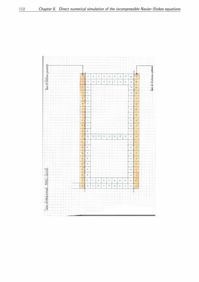
112 Chapter 8. Direct numerical simulation of the incompressible Navier–Stokes equations

8.5. Detailed description of a notional two-dimensional MAC grid 113
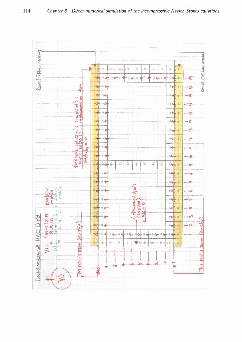
114 Chapter 8. Direct numerical simulation of the incompressible Navier–Stokes equations

Chapter 9
Simplified model problems involving
Poisson and Helmholtz equations
Overview
We consider analytical solutions to a two-dimensional diffusion problem. The reason for examining
this particular problem are manifold: it is a minimal model that nonetheless has a small amount
of complexity sufficient to warrant the use of a number of interesting numerical methods. Also,
analytical solutions in this section will be used as benchmarks for future numerical simulation studies.
Throughout this chapter and beyond, the problem considered in herein be referred to as the model
diffusion equation.
9.1 Boundary conditions – review
For this discussion, let
∂C
∂t= a(x, t)
∂2C
∂x2+ b(x, t)
∂C
∂x+ c(x, t)C + d(x, t), x ∈ (0, L), t > 0,
be a parabolic partial differential equation in one space dimension, on x ∈ (0, L), with smooth initial
conditions
C(x, t = 0) = Cinit(x), x ∈ [0, L].
Then the following boundary conditions are possible.
115
116 Chapter 9. Simplified model problems involving Poisson and Helmholtz equations
1. Dirichlet conditions The function C(x, t > 0) is specified on the boundaries:
C(0, t > 0) = g1(t),
C(L, t > 0) = g2(t).
If the functions g1 = g2 = 0, then we have homogeneous Dirichlet conditions:
C(0, t > 0) = 0,
C(L, t > 0) = 0.
2. Neumann conditions: The derivative Cx(x, t > 0) is specified on the boundaries:
Cx(0, t > 0) = g1(t),
Cx(L, t > 0) = g2(t).
If the functions g1 = g2 = 0, then we have homogeneous Neumann conditions, corre-
sponding to no flux through the boundaries.
3. Mixed conditions: As the name suggests, this set is a mixture of Dirichlet and Neumann
conditions:
α1Cx(0, t > 0) + α2C(0, t > 0) = g1(t),
α3Cx(L, t > 0) + α4C(L, t > 0) = g2(t).
4. Periodic boundary conditions: The function C(x, t > 0) has the same value on either
boundary point:
C(0, t) = C(L, t), t > 0.
In practice, these are not very realistic boundary conditions but they are used in numerical
experiments because they are easy to implement. However, they can be used to mimic an
infinite domain, if the periodic length L is made long enough.
9.2 The model diffusion equation
We are interested in solving the following partial differential equation (PDE) for diffusion, given here
in non-dimensional form as follows:
∂C
∂t= ∇2C + s(x, z), (x, z) ∈ Ω, (9.1a)
9.3. Physical interpretation 117
where
Ω = (0, Lx)× (0, 1), (9.1b)
and ∇2 = ∂2x + ∂2
z is the Laplacian. The partial differential equation is subject to the following
boundary conditions:∂C
∂z= 0, z = 0, z = 1, (9.1c)
together with periodic boundary conditions in the x direction:
C(x = 0, z, t) = C(x = Lx, z, t). (9.1d)
Finally, an initial condition is prescribed:
C(x, z, t = 0) = Cinit(x, z), (x, z) ∈ Ω, (9.1e)
where Cinit(x, z) is a continuous function. Here, the system of equations (10.1) is made non-
dimensional on the channel depth Lz (herein set to unity), and the diffusive timescale τ = L2z/D,
where D is the diffusion coefficient.
9.3 Physical interpretation
Physically, Equation (10.1) is a model for diffusion of particles in the presence of a source. The
amount of matter in the system changes over time, due to contributions from the source s(x, y, z).
There are no contributions from the boundary conditions. For, consider the following evolution
equation for the total system mass
M =
∫Ω
d2xC(x, z, t).
We have
dM
dt=
∫Ω
d2x∂C
∂t,
=
∫Ω
d2x[∇2C + s(x, z)
],
=
∫Ω
d2x s(s, z) +
∫∂Ω
d`n · ∇C,

118 Chapter 9. Simplified model problems involving Poisson and Helmholtz equations
where ∂Ω is the boundary of the set Ω, d` is a line element on the boundary, and n is the outward-
pointing unit normal to ∂Ω. We compute∫∂Ω
dAn · ∇C =
∫ Lx
0
dx∂C
∂z
∣∣∣∣z=1
−∫ Lx
0
dx∂C
∂z
∣∣∣∣z=0
+
∫ Lz
0
dz∂C
∂x
∣∣∣∣x=Lx
−∫ Lz
0
dz∂C
∂x
∣∣∣∣x=0
.
However, all of these terms cancel, either because of the no-flux boundary condition (∂C/∂z)(z =
0, 1) = 0, or because of periodicity, meaning that
dM
dt= LxLz〈s〉, 〈s〉 :=
1
LxLz
∫Ω
d2x s(s, z). (9.2)
9.4 Decomposition
In view of the formula (9.2), it is sensible to split the solution into two parts:
C = 〈C〉(t) + C ′(x, z, t), s = 〈s〉+ s′(x, z).
By linearity,
∂
∂t〈C〉 = ∇2〈C〉+ 〈s〉,
∂C ′
∂t= ∇2C ′ + s′.
Indeed, the solution to the mean contribution is known:
〈C〉(t) = 〈C〉(t = 0) + 〈s〉t = 〈Cinit〉+ 〈s〉t.
while the PDE for the fluctuations inherits all the properties of the basic PDE (10.1), such that
∂C ′
∂t= ∇2C ′ + s′(x, z), (x, z) ∈ Ω, (9.3a)
subject to the following boundary conditions:
∂C ′
∂z= 0, z = 0, z = 1, (9.3b)
together with periodic boundary conditions in the x-direction:
C ′(x = 0, z, t) = C ′(x = Lx, z, t). (9.3c)
9.5. Analytical solution 119
Finally, an initial condition is prescribed:
C ′(x, z, t = 0) = Cinit(x, z)− 〈Cinit〉, (x, z) ∈ Ω, (9.3d)
9.5 Analytical solution
We prove the following theorem:
Theorem 9.1 Equation (9.3) has at least one smooth solution, namely
C ′(x, z, t) =∞∑n=1
∞∑i=−∞
e−k
2int
[ain(0)− sin
k2in
]+sink2in
ei[(2π/Lx)ix] cos
(nπz
Lz
), (9.4a)
where
ain(0) =2
LxLz
∫ Lx
0
∫ Lz
0
d2x e−i[(2π/Lx)ix] cos
(nπz
Lz
)[Cinit(x, z)− 〈Cinit〉] , (9.4b)
and where we have restored the definition of Lz for clarity’s sake.
Proof: Take Equation (9.1a), multiply by cos(nπz/Lz) (with n = 1, 2, · · · ) and integrate with
respect to z. The result is
∂t
∫ Lz
0
C ′ cos
(nπz
Lz
)dz = ∂2
x
∫ Lz
0
C ′ cos
(nπz
Lz
)dz +
∫ Lz
0
(∂2C ′
∂z2
)cos
(nπz
Lz
)dz
+
∫ Lz
0
s(x, z) cos
(nπz
Lz
)dz.
We call
Cn(x, t) :=2
Lz
∫ Lz
0
C ′(x, t) cos
(nπz
Lz
)dz, sn(x) :=
2
Lz
∫ Lz
0
s(x, z) cos
(nπz
Lz
)dz;
hence, we have∂Cn∂t
= ∂2xCn +
2
Lz
∫ Lz
0
(∂2C ′
∂z2
)cos
(nπz
Lz
)dz + sn(x). (9.5)

120 Chapter 9. Simplified model problems involving Poisson and Helmholtz equations
Consider now the following (with kn = nπ/Lz):∫ Lz
0
(∂2C ′
∂z2
)cos
(nπz
Lz
)dz =
∫ Lz
0
∂
∂z
[cos
(nπz
Lz
)∂C ′
∂z
]+ kn sin
(nπz
Lz
)∂C ′
∂z
dz,
=
[cos
(nπz
Lz
)∂C ′
∂z
]z=Lzz=0
+ kn
∫ Ly
0
sin
(nπz
Lz
)∂C ′
∂zdz,
= 0 + kn
∫ Lz
0
sin
(nπz
Lz
)∂C ′
∂zdz,
= kn
∫ Lz
0
∂
∂z
[sin
(nπz
Lz
)C ′]− kn cos
(nπz
Lz
)C ′
dz,
=
[sin
(nπz
Lz
)C ′]z=Lzz=0
− k2n
∫ Lz
0
cos
(nπz
Lz
)C ′(x, z, t) dz.
Hence,
2
Lz
∫ Lz
0
(∂2C ′
∂z2
)cos
(nπz
Lz
)dz = −k2
n (2/Lz)
∫ Lz
0
cos
(nπz
Lz
)C ′(x, z, t) dz = −k2
nCn.
Thus, Equation (9.1a) is transformed – via Equation (9.5) to
∂Cn∂t
+ k2nCn = ∂2
xCn + sn(x). (9.6)
However, this is now a standard diffusion problem in one (periodic) dimension, which can be solved
by standard Fourier-series methods: we propose
Cn(x, t) =∞∑
i=−∞
ain(t)ei[(2π/Lx)ix];
we also decompose sn(x) as
sn(x) =∞∑
i=−∞
sinei[(2π/Lx)ix].
Thus, the following amplitude equations are obtained:
daindt
= −k2inain + sin, (9.7)
where
kin =
[(2π
Lx
)2
i2 +
(π
Lz
)2
n2
]1/2
.

9.5. Analytical solution 121
Equation (9.7) has solution
ain(t) =
e−k2int[ain(0)− sin
k2in
]+ sin
k2ijn, kin 6= 0,
a0(0) + s0t, kin = 0,
where the second case follows because kin = 0 if and only if i = n = 0. However, this case is ruled
out because n 6= 0. Thus, the solution for Cn(x, t) is therefore
Cn(x, t) =∞∑
i=−∞
e−k
2int
[ain(0)− sin
k2in
]+sink2in
ei[(2π/Lx)ix].
We now note that a cosine transform has been taken in the z-direction:
Cn(x, t) =2
Lz
∫ Lz
0
cos
(nπz
Lz
)C ′(x, z, t) dz, n 6= 0.
However, since cos
(nπz
Lz
)∞n=1
is a basis for mean-zero continuous functions whose first derivative vanishes at z = 0, Lz, meaning
that the cosine transform can be reversed:
C ′(x, z, t) =∞∑n=1
Cn(x, t) cos
(nπz
Lz
).
Hence,
C ′(x, z, t) =∞∑n=1
∞∑i=−∞
e−k
2int
[ain(0)− sin
k2in
]+sink2in
ei[(2π/Lx)ix] cos
(nπz
Lz
).
Finally, it is of interest to determine the coefficients aijn(0). We have
Cinit(x, z)− 〈Cinit〉 =∞∑n=1
∞∑i=−∞
aij(0)ei[(2π/Lx)ix] cos
(nπz
Lz
),
hence, by Fourier transformation,
ain(0) =2
LxLz
∫ Lx
0
∫ Lz
0
d2x e−i[(2π/Lx)ix] cos
(nπz
Lz
)[Cinit(x, z)− 〈Cinit〉] .
(the factor of 2 comes from the cosine series). Having constructed a solution to Equation (9.3), it
is also the case that this is the only such smooth solution:
Theorem 9.2 Equation (9.4) is the unique smooth solution of Equation (9.3).
122 Chapter 9. Simplified model problems involving Poisson and Helmholtz equations
Exercise 9.1 Prove Theorem (9.2).
9.6 The model Poisson problem
We shall also consider a simpler problem than the diffusion problem posed previously. It will be
referred to throughout the course as the model Poisson problem, given here as follows:
∇2C0 + s(x, z) = 0, (x, z) ∈ Ω, (9.8a)
where
Ω = (0, Lx)× (0, 1), (9.8b)
with boundary conditions∂C0
∂z= 0, z = 0, z = 1, (9.8c)
and
C0(x = 0, z, t) = C0(x = Lx, z, t). (9.8d)
9.7 Solvability condition and explicit solution
Consider Equation (9.8a). Integrate both sides over x and z and apply the boundary conditions on
C. The result is
0 =
∫ Lx
0
dx
∫ Lz
0
dz s(x, z).
Thus, in order to get a self-consistent solution, we require that the source should have zero mean:
〈s〉 :=1
LxLz
∫ Lx
0
dx
∫ Lz
0
dz s(x, z) = 0.
This is referred to as the solvability condition.
Assuming that Equation (9.8) satisfies the solvability condition, a solution is available through a
Fourier-cosine series:
C0(x) =∞∑n=1
∞∑i=−∞
sink2in
ei[(2π/Lx)ix] cos
(nπz
Lz
), (9.9)
where kin and sin are defined as in Section 9.2.
9.8. Relation between model diffusion and Poisson problems 123
9.8 Relation between model diffusion and Poisson problems
It is clear from Equation (9.9) that
limt→∞
C ′(x, z, t) = C0(x, z),
where C ′(x, z, t) (LHS) is the fluctuating part of the solution of the model diffusion problem, and
C0(x) (RHS) here denotes the solution of the model Poisson problem. Thus, the following theorem
is shown:
Theorem 9.3 Let 〈s〉 = 0 in the model diffusion equation. Then the solution C(x, z, t) of the
model diffusion equation – given smooth initial data – converges to the solution of the model
Poisson problem, as t→∞:
limt→∞
C(x, z, t) = C0(x, z), ∇2C0(x, z) + s(x, z) = 0.
Exercise 9.2 Prove Theorem 9.3 using a second approach: show first that
∂
∂t(C − C0) = ∇2 (C − C0) ,
and hence show that
limt→∞
C(x, z, t) = C0(x, z). (9.10)
Non-uniqueness of solutions
Consider again the model Poisson problem with solution (9.9). It is clear that C0 + Const. is also
a solution, since ∇2(Const.) = 0, and C0 + Const. also satisfies the boundary conditions (hybrid
periodic–Neumann). The solution (9.9) is therefore not unique. This is because the operator ∇2,
equipped with the hybrid periodic–Neumann boundary conditions has a non-trivial kernel – the set
of all constant functions is a one-dimensional vector subspace and is the non-trivial kernel of the
PDE.
Exercise 9.3 What happens to the kernel of ∇2 if the boundary conditions are modified to
be a mixture of periodic BCs in the x-direction and homogeneous Dirichlet conditions in the
z-direction?

124 Chapter 9. Simplified model problems involving Poisson and Helmholtz equations

Chapter 10
Simplified model problems – numerical
setup
Overview
In this chapter we consider numerical solutions of the model equations We introduce centred differ-
encing in space as a way of approximating the Laplace operator numerically. For the model diffusion
equation, we introduce Crank–Nicholson temporal discretization as a way of discretizing the tempo-
ral derivative ∂/∂t. Crank–Nicholson is a so-called implicit method, which means that a certain
equation must be inverted in order to evolve the numerical solution forward in time, stepping from
one time step to the next. For this reason, Jacobi iteration is introduced as a method for solving
such implicit (linear) equations.
10.1 Diffusion equation
We are interested in solving the PDE from Chapter 8, recalled here to be
∂C
∂t= ∇2C + s(x, z), (x, z) ∈ Ω, (10.1a)
where
Ω = (0, Lx)× (0, 1), (10.1b)
and ∇2 = ∂2x + ∂2
z is the Laplacian. The partial differential equation is subject to the following
boundary conditions:∂C
∂z= 0, z = 0, z = 1, (10.1c)
125

126 Chapter 10. Simplified model problems – numerical setup
together with periodic boundary conditions in the x- and y-directions:
C(x = 0, z, t) = C(x = Lx, z, t). (10.1d)
Finally, an initial condition is prescribed:
C(x, z, t = 0) = Cinit(x, z), (x, z) ∈ Ω, (10.1e)
where Cinit(x, z) is a continuous function. Here, the system of equations (10.1) is made non-
dimensional on the channel depth Lz (herein set to unity), and the diffusive timescale τ = L2z/D,
where D is the diffusion coefficient.
10.2 The discretization
We discretize the PDE and compute its approximate numerical solution on a discrete grid:
xi = (i− 1)∆x, i = 1, · · ·nx,
zj = (j − 1)∆z, j = 1, · · ·nz,
such that
(nx − 1)∆x = Lx, ∆x = Lx/(nx − 1),
and similarly, ∆z = Lz/(nz − 1). The PDE is also discretized in time, such that the solution is
only available at discrete points in time tn = n∆t, with n = 0, 1, · · · . The solution at tn and
x = (i∆x, y∆j) is written as Cnij. The diffusion operator in the PDE (10.1) is approximated by
centred differences:
(∇2C
)ij≈ Ci+1,j + Ci−1,j − 2Cij
∆x2+Ci,j+1 + Ci,j−1 − 2Cij
∆z2:= D(Cij)
i = 2, 3, · · · , nx − 1, j = 2, 3, · · · , nz − 1.
The discretization in time is done using a Crank–Nicholson scheme:
Cn+1ij − Cn
ij
∆t= 1
2
[D(Cn
ij) +D(Cn+1ij )
]+ sij, i = 2, 3, · · · , nx − 1, j = 2, 3, · · · , nz − 1.

10.3. Jacobi method 127
Re-arrange:
[1− 1
2∆tD
] (Cn+1ij
)=[1 + 1
2∆tD
] (Cnij
)+ ∆tsij,
i = 2, 3, · · · , nx − 1, j = 2, 3, · · · , nz − 1. (10.2)
On the left-hand side, the quantity[1− 1
2∆tD
]is in fact a matrix operator, and the solution is
available only in implicit form: an inversion needs to be performed to extract Cn+1ij from this implicit
equation:
Cn+1ij =
[1− 1
2∆tD
]−1 [1 + 1
2∆tD
] (Cnij
)+ ∆tsij
. (10.3)
The implicit equation (10.2) is written out in more detail now:
(1 + ax + ay)Cn+1ij −1
2ax(Cn+1i+1,j + Cn+1
i−1,j
)−1
2az(Cn+1i,j+1 + Cn+1
i,j−1
)=[1 + 1
2∆tD
] (Cnij
)+sij := RHSnij,
where ax = ∆t/∆x2 and az = ∆t/∆z2. Tidy up:
(1 + ax + ay)Cn+1ij − 1
2ax(Cn+1i+1,j + Cn+1
i−1,j
)− 1
2az(Cn+1i,j+1 + Cn+1
i,j−1
)= RHSnij. (10.4)
This is an implicit equation for Cn+1ij that we must now endavour to solve.
10.3 Jacobi method
The focus of this course is on the use of iterative methods to solve problems such as Equa-
tion (10.3) or equivalently, Equation (10.4). The idea is to make an initial guess for the solution,
plug this into some algorithm for refining the guess, and continue until this iterative procedure
converges.
The simplest and most naive iterative method os the so-called Jacobi method. Let v ≡ Cn+1 be
the array to be found by solving Equation (10.3):
(1 + ax + ay) vij − 12ax (vi+1,j + vi−1,j)− 1
2az (vi,j+1 + vi,j−1) = RHSij.
This can be re-arranged simply as
vij =12ax (vi+1,j + vi−1,j) + 1
2az (vi,j+1 + vi,j−1) + RHSij
1 + ax + az. (10.5)
The idea of the Jacobi method is to take a guess for v, say vN , and to create a new guess vN+1 via
the formula
vN+1ij =
12ax(vNi+1,j + vNi−1,j
)+ 1
2ay(vNi,j+1 + vNi,j−1
)+ RHSij
1 + ax + ay. (10.6)
128 Chapter 10. Simplified model problems – numerical setup
If this iterative scheme converges, then limN→∞ vN = limN→∞ v
N+1, and the approximate solutions
vN and vN+1 can be replaced in Equation (10.6) with some identical array v∗, thereby forcing
Equation (10.6) to be identical to Equation (10.5).
10.4 Boundary conditions
The idea to solve the PDE (10.1a) is to do implement a Crank–Nicholson-centred difference scheme
at interior points. Inversion of the resulting implicit problem is then achieved by the Jacobi method.
However, this approach can only be used at interior points
i = 2, 3, · · · , nx − 1, j = 2, 3, · · · , nz − 1.
At boundary points, the boundary conditions are enforced: ∂C/∂z = 0 at z = 0, 1, and periodic
boundary conditions in the x-direction. These are implemented numerically in a straightforward
fashion. The Neumann conditions at z = 0, Lz are implemented as
Ci,j=1 = Ci,j=2, Ci,j=ny = Ci,j=ny−1,
while the periodicity conditions at x = 0, Lx are implemented as follows
• i = 1: C(i− 1, j) = C(nx − 1, j),
• i = nx: C(i+ 1, j) = C(2, j).
Thus, the points i = 1 and i = nx are identified.
10.5 The algorithm
We can now assemble an algorithm to solve Equation (10.1a) numerically:
1. Set up a discretization scheme with ∆x, ∆z, and ∆t defined by the user. Also, prescribe an
initial condition Cinit(x, z) and a source function s(x, z).
2. Obtain Cn=1ij from C0
ij at interior points using centred differences, the Crank–Nicholson tem-
poral discretization, and Jacobi iteration.
3. Implement many iterations of the Jacobi method, until the method has converged to some
user-defined tolerance.
4. Implement the boundary conditions on Cn=1.
10.5. The algorithm 129
5. Repeat steps 2–4 for the desired number of timesteps.
Matlab codes to implement this problem are given in Appendix A.

Chapter 11
Analysis of numerical setup
Overview
The idea of this chapter is to take a generic linear problem Ax = b, and to formulate a sufficient
condition on A that guarantees the success of the Jacobi iterative method. It turns out that
this sufficient condition is something called diagonal dominance, which means that the diagonal
elements of A should be large (in some sense) compared to the off-diagonal ones.
11.1 Generic discussion
Consider the Jacobi scheme for solving
Av = b, (A)ij = aij ∈ R.
The idea is to write A = D + R, where
D = diag (a11, a22, · · · , ann) , n ∈ N,
and where
R = A−D.
Then, the iterations vN ,vN+1 that generate approximate solutions are obtained as follows:
DvN+1 = −RvN + b,
130

11.1. Generic discussion 131
for a given starting-guess v0. Assume that
limN→∞
= v∗.
Thus,
DvN+1 = −RvN + b,
Dv∗ = −Rv∗ + b.
Subtract:
D(vN+1 − v∗
)= −R
(vN − v∗
),
or
DrN+1 = −RrN , (11.1)
where rN = vN − v∗ is the residual vector at level N . Take L2 vector norms on both sides:
‖rN+1‖2 = ‖D−1RrN‖2.
Now, use the L2 operator norm:
‖rN+1‖2 ≤ ‖D−1R‖2‖rN‖2.
Telescope this result:
‖rN‖2 ≤(‖D−1R‖2
)N ‖r0‖2.
By requiring that ‖D−1R‖2 < 1, we obtain
limN→∞
‖rN‖2 = 0,
hence
limN→∞
rN = 0,
hence
limN→∞
vn = v∗.

132 Chapter 11. Analysis of numerical setup
Thus, we have shown the following theorem:
Theorem 11.1 A sufficient condition for the convergence of the Jacobi iteration algorithm
DvN+1 = −RvN + b, vN=0 = v0,
is the following bound on the L2 operator norm:
‖D−1R‖2 < 1. (11.2)
For systems with entries on the diagonal that are relatively large (in absolte-value terms) compared
to entries off the diagonal, this constraint is usually satisfied, and the Jacobi iteration converges.
However, this is a relatively vague criterion, which is of limited use. In addition, the L2 operator norm
is difficult to compute numerically, so in practice it is not known a priori – using Theorem (11.1)
alone – whether the Jacobi method will converge. For that reason, we need a more rigorous notion
of diagonal dominance.
11.2 Diagonal dominance
Definition 11.1 (L∞ matrix norm) Let M ∈ Rn×n. Then
‖M‖∞ = sup‖x‖∞=1
‖Mx‖∞,
where ‖x‖∞ denotes the ordinary L∞ norm for vectors: for x = (x1, · · · , xn) ∈ Rn,
‖x‖∞ = maxi|xi|.
11.2. Diagonal dominance 133
Lemma 11.1 (Consistency of the L∞ norm) Let M1 and M2 be square matrices in Rn×n.
Then
‖M1M2‖∞ ≤ ‖M1‖∞‖M2‖∞.
Proof: It suffices to consider the case with ‖M1M2‖∞ 6= 0.
‖M1M2‖∞ = sup‖x‖∞=1
‖M1M2x‖∞,
= ‖M1M2x0‖∞,
= ‖M1y‖∞, y = M2x0 6= 0,
=
(‖M1y‖∞‖y‖∞
)‖y‖∞,
≤[supy 6=0
(‖M1y‖∞‖y‖∞
)]‖y‖∞,
= ‖M1‖∞‖y‖∞,
= ‖M1‖∞‖M2x0‖∞,
≤ ‖M1‖∞‖M2‖∞.
Definition 11.2 Let M ∈ Rn×n. The spectral radius ρ(M) refers to that M-eigenvalue with
maximal absolute value:
ρ(M) = maxi
(|λi|) , Mxi = λixi.

134 Chapter 11. Analysis of numerical setup
Theorem 11.2 (Bound on the spectral radius) Let M ∈ Rn×n. Then
ρ(M) ≤ ‖M‖∞.
Proof: Let Mx = λx, with x 6= 0. Let
X =
| |x · · · x
| |
.
Thus,
MX = λX.
Take L∞ norms on both sides:
|λ|‖X‖∞ = ‖Mx‖∞ ≤ ‖M‖∞‖X‖∞,
hence
|λ| ≤ ‖M‖∞,
for any eigenvalue λ, and the result is shown:
ρ(M) ≤ ‖M‖∞.
Now, by this stage, I am tired of proving theorems, so I shall simply state this last and crucial
theorem:
Theorem 11.3 Let M ∈ Rn×n. Then
‖M‖∞ = maxi
(n∑k=1
|mik|
). (11.3)
Note the sum over columns!

11.2. Diagonal dominance 135
Putting it all together
We now apply these results to M = D−1R. In view of Theorem 11.2 and Theorem 11.3, we have
ρ(D−1R
)≤ ‖D−1R‖∞ = max
i
(n∑k=1
|(D−1R)ik|
)
But
D−1R =
0 a12
a11· · · a1,n−1
a11
a1na11
...an1ann
· · · an,n−1
ann0
,
hence
ρ(D−1R
)≤ ‖D−1R‖∞ = max
i
1
|aii|
n∑k=1k 6=i
|aik|
.
This motivates a definition:
Definition 11.3 A matrix A ∈ Rn×n is diagonally dominant if
1
|aii|
n∑k=1k 6=i
|aik| < 1,
for each i = 1, 2, · · · , n.
Along the way, we have established the following facts for a diagonally-dominant matrix:
Theorem 11.4 Let A ∈ Rn×n be diagonally dominant. Then
ρ(D−1R
)≤ ‖D−1R‖∞ = max
i
1
|aii|
n∑k=1k 6=i
|aik|
< 1,
where D and R have their usual meanings.

136 Chapter 11. Analysis of numerical setup
We now consider a final theorem:
Theorem 11.5 Let Av = b be a linear problem, where A ∈ Rn×n is diagonally dominant. Then
the Jacobi iteration method converges.
Proof: Start with the definition of the Jacobi residuals, Equation (11.1) or, equivalently,
rN+1 = −D−1RrN , (11.4)
Telescope the result:
rN = (−1)N(D−1R
)Nr0.
Write
D−1R = P−1JP,
where J is the Jordan normal form associated with D−1R. We have
rN = (−1)N(−D−1R
)Nr0,
= (−1)N(P−1JP
)Nr0,
= (−1)N(P−1JNP
)r0.
We now use the fact that ρ(D−1R) ≤ ‖D−1R‖∞ < 1 as in the hypothesis of the theorem. Thus,
all the eigenvalues have modulus less than one. Hence, each block in the Jordan matrix, raised to
the N th power, tends to zero as N →∞. It follows that
limN→∞
JN = 0. (11.5)
Therefore, finally,
limN→∞
rN = 0.
11.3 Operation count
An elementary (non-iterative) method of solving linear problems is Gaussian elimination. The op-
eration count of Gaussian elimination is O(n3), meaning that the number of operations (addition,
multiplication etc.) required to invert the matrix is proprtional to the cube of the size of the matrix.
This can be regarded as a relatively good performance result, since it compares very favourably with
the operation count of determinant-type calculations, the latter being another candidate method for
matrix inversion. However, for massive calculations (e.g. n ∼ 106), even the relatively good per-
formance of Gaussian elimination (O(n3)) is not satisfactory. For such large calculations, iterative
methods such as the Jacobi scheme are preferred; clearly in such iterative methods, the count is
11.4. SOR 137
O(ncn2), where nc is the number of iterations required for the method to converge, with nc n
for n large.
Recall theorem (11.4) above: given a diagonally-dominant problem Ax = b, the Jacobi iteration
method will converge. In this module, we are always working with such systems. Thus, the Jacobi
method will always work for us. However, its convergence is quite poor. In other words, a relatively
large number of iterations is required in order to obtain a sufficiently converged solution. In this
section we outline a new method. Superficially, it is a straightforward extension of the Jacobi
method; however, on deeper reflection, the improved method represents a conceptual leap. This is
the method of successive over-relaxation (SOR).
11.4 SOR
Start with the generic problem
Ax = b.
Recall the Jacobi solution:
DvN+1 = −RvN + b.
In index notation,
vN+1i =
1
aii
(−
n∑j=1
RikvNk + bi
). (11.6)
The idea behind SOR is to retrospectively improve the ‘old guess’ vN that goes into formulating the
‘new guess’. If the ‘old guess’ can be retrospectively improved, then this makes the new guess even
better. To do this, the right-hand side of the Jacobi equation (11.6) is updated with just-recently-
created values of vN+1. Where this is not possible, the old values of vN are used. The result is the
following iterative scheme:
vN+1i = − 1
aii
i−1∑k=1
RikvN+1k − 1
aii
n∑k=i
RikvNk +
biaii. (11.7)
But Rii = 0, and Rij = aij otherwise. Hence, Equation (11.7) can be replaced by
vN+1i =
1
aii
[bi −
i−1∑k=1
aikvN+1k −
n∑k=i+1
aikvNk
]. (11.8)
Equation (11.8) is not yet optimal (however, it is already the Gauss–Seidel method for solving a
linear system). Instead, we introduce an extra degree of freedom, which allows us to weight how
much or how little retrospective improvement of the old guess is implemented in the (N + 1)th
138 Chapter 11. Analysis of numerical setup
iteration step. This is done by a simple modification of Equation (11.8):
vN+1i = (1− ω) vNi +
ω
aii
[bi −
i−1∑k=1
aikvN+1k −
n∑k=i+1
aikvNk
](11.9a)
The factor ω is restricted to the range
0 < ω < 2; (11.9b)
this preserves the diagonal-dominance of the system and hence ensures convergence. The exact
choice of ω is made by trial-and-error in order to speed up convergence.
Exercise 11.1 Re-write the diffusion and Poisson subroutines from Chapter 10 using the SOR
method instead of the Jacobi method. Determine heuristically the approrpiate values for the
relaxation parameter for both the Helmholtz and Poisson problems.

Chapter 12
Elements of turbulence theory
Overview
We give a qualitative definition of turbulence and introduce the phenomenological Kolmogorov
theory of the turbulent spectrum in three dimensions.
We discuss averaging techniques to reduce the complexity of the fully turbulent Navier–Stokes
equations. These are exemplified in the theory of wall-bounded turbulent flows and the famous
‘law of the wall’, Finally, we introduce large-eddy simulations as a half-way house between the full
direct numerical simulation (DNS) of the turbulent Navier–Stokes equations and the relatively crude
averaging techniques. At the end of the chapter, the students will be asked to carry out a large-eddy
simulation of a wall-bounded flow and to extract various turbulent statistics from the simulation
data.
Much of the description in this chapter is taken quite directly from the book by Pope [Pop00].
12.1 Turbulence phenomenology
Turbulence is defined here as a particular kind of fluid motion characterized by a velocity field that
varies in space and time in a complicated way, with the following two essential features:
• In the spatial domain, turbulent motion is characterized by the presence of many lengthscales,
from the domain scale (whereupon an external forcing is typically applied), down to small
lengthscales where viscous motion dominates.
• In the temporal domain, the velocity field is characterized by a non-periodic, non-constant
variation in time (i.e. chaotic motion).
139

140 Chapter 12. Elements of turbulence theory
Note that by itself the existence of a chaotic temporal dynamics is not sufficient to characterize
turbulence: it is possible for example to observe chaotic advection in laminar flows [Are84].
Because turbulence is generated from an underlying deterministic set of equations (i.e. the Navier–
Stokes equations), it can be characterized in a deterministic fashion. However, the system contains
a large number of degrees of freedom. Focusing for definiteness (but without loss of generality) on
the case wherein the domain is a periodic box, the Fourier modes of the system form a complete
discrete set of degrees of freedom, all interacting nonlinearly to produce the complicated dynamics
alluded to in the definition. In this way, the discrete modes can be thought of as analogous to
particles in a gas: each particle can be thought of as obeying deterministic Newtonian dynamics,
but on the macroscopic level, a statistical description of the collection of gas particles (all possibly
interacting) is possible and indeed, desirable. Thus, in the case of a turbulent velocity field, we
introduce a statistical description of the flow, characterized by a probability distribution function
f(V ;x, t) for the velocity field U = (U1, U2, U3), such that
Prob
a1 < U1 < b1
a2 < U2 < b2
a3 < U3 < b3
;x, t
=
∫ b1
a1
∫ b2
a2
∫ b3
a3
f(V ;x, t) dV1 dV2 dV3.
The average velocity is therefore
〈U(x, t)〉 =y
d3V f(V ;x; t)V ,
and the fluctuation velocity is defined as
u(x, t) = U(x, t)− 〈U(x, t)〉.
The probability distribution function relates to quantities evaluated at a single point in space and
time. Of interest also are so-called N -point statistics: let
fN(V (1),x(1), t(1);V (2),x(2), t(2); · · · ;V (N),x(N), t(N)
)be the joint probability distribution for the velocity random-variable V at space-time points
(x(1), t(1)), · · · , (x(N), t(N)).
It should be noted that turbulent velocity fields are found not to be Gaussian: a Gaussian field is
be fully characterized by the mean 〈U(x, t)〉 and by the covariances 〈ui(x(1), t(1))uj(x(2), t(2))〉.

12.1. Turbulence phenomenology 141
The random field U(x, t) is statistically stationary if the N -point correlation function is invariant
under a shift in time:
fN(V (1),x(1), t(1) + T ;V (2),x(2), t(2) + T ; · · · ;V (N),x(N), t(N) + T
)= fN
(V (1),x(1), t(1);V (2),x(2), t(2); · · · ;V (N),x(N), t(N)
).
Similarly, U (x, t) is statistically homogeneous if the N -point correlation function is invariant
under a shift in the coordinate:
fN(V (1),x(1) + y, t(1);V (2),x(2) + y, t(2); · · · ;V (N),x(N) + y, t(N)
)= fN
(V (1),x(1), t(1);V (2),x(2), t(2); · · · ;V (N),x(N), t(N)
).
Then, in particular, the distribution function f(V ;x, t) is itself translation invariant, and we obtain
〈U(x, t)〉 =y
d3V f(V ;x; t)V ,y
d3V f(V ;x+ y; t)V = 〈U(x+ y, t)〉
for all y ∈ R3 and hence, the average velocity field is constant in space. Obviously this is quite
restrictive: too restrictive in fact. We therefore define a homogeneous turbulence to correspond
to a turbulent velocity field wherein the N -point distribution function for the fluctuations is ho-
mogeneous (translation invariant). Later on, in the context of Reynolds-averaging, we shall show
that for homogeneous turbulence, the mean strain rates (∂/∂xj)〈Ui〉 are uniform (but can depend
on time).
Because the distributional averages, e.g. 〈U(x, t)〉 =t
dV f(V ;x, t)V are equivalent to ensem-
ble averages, e.g.
〈U(x, t)〉 = limN→∞
1
N
N∑i=1
U (i)(x, t),
where the superscript denotes the ith realisation of the velocity field in a set of N identical experi-
ments, it follows that the averaging and the derivatives commute, i.e.
∂
∂t〈Ui〉 =
⟨∂Ui∂t
⟩, (12.1a)
and∂
∂xj〈Ui〉 =
⟨∂Ui∂xj
⟩. (12.1b)
These facts will be crucial in the next section concerning Reynolds-averaging.

142 Chapter 12. Elements of turbulence theory
12.2 Reynolds averaging
We take the instantaneous Navier–Stokes equations and we perform the averaging operation, using
the properties 12.1. We obtain
∂
∂t〈Ui〉+ 〈U · ∇Ui〉 = −∇〈p〉+
1
Re∇2〈Ui〉.
The problematic term here is the quantity
〈U · ∇Ui〉 = 〈Uj∂Ui∂xj〉,
=
⟨[〈Uj〉+ uj]
[∂
∂xj〈Ui〉+
∂ui∂xj
]⟩,
=
⟨〈Uj〉
∂
∂xj〈Ui〉
⟩+
⟨〈Uj〉
∂ui∂xj
⟩+
⟨uj
∂
∂xj〈Ui〉
⟩+
⟨uj∂ui∂xj
⟩.
We use the obvious properties
〈〈a〉〉 = 〈a〉, 〈ui〉 = 0,
to obtain
〈U · ∇Ui〉 = 〈Uj〉∂
∂xj〈Ui〉+
⟨uj∂ui∂xj
⟩,
= 〈U〉 · ∇〈Ui〉+∂
∂xj〈uiuj〉.
We introduce
τij = −〈uiuj〉
as the Reynolds stress tensor. Then, the averaged equations of motion become
∂
∂t〈Ui〉+ 〈U〉 · ∇〈Ui〉 = −∇〈p〉+
∂τij∂xj
+1
Re∇2〈Ui〉, ∇ · 〈U〉 = 0. (12.2)
These are the Reynolds-averaged Navier–Stokes (RANS) equations.
12.3 Closure problem
The Reynolds stresses cannot be determined a priori – this is the closure problem of turbulence.
Certainly, one can write down a transport equation for the Reynolds stresses themselves, e.g.(∂
∂t+ 〈U〉 · ∇
)τij = · · · ,

12.4. Eddy-viscosity model for channel flows 143
but the right-hand side will involve tensors of at least rank three built out of the fluctuating veloc-
ities. To constitute these tensors, one needs a further transport equation and so on, ad infinitum.
Additional knowledge from outside the set of RANS equations is needed to break this infinite chain
of equations. At the very simplest level, this is done by constitutive modelling of the Reynolds
stress tensor; at higher levels of detail, tensors of higher rank are modelled and fed back into the
transport equations for the tensors of lower rank, thereby closing the problem. Consideration is given
herein to the simple approach.
Eddy viscosity model
In the simplest possible closure model, the Reynolds stresses themselves are modelled. The concep-
tual approach is to identify the total stress tensor in the RANS equations:
Tij = −pδij +Re−1 (∂i〈Uj〉+ ∂j〈Ui〉)− 〈uiuj〉,
and to assume an analogy between molecular diffusion and the effects of turbulence. Namely, on a
small scale, one pictures a fluid parcel undergoing thermal fluctuations due to molecular diffusion,
and further fluctuations due to the small-scale motions of the neighbouring turbulent eddies. One
assumes that these effects are similar, such that on average, the effects of the turbulence can be
modelled as though they were somehow viscous in nature, with
τij = νT (∂i〈Uj〉+ ∂j〈Ui〉) ,
where νT is the eddy viscosity. Dimensional analysis then suggests
νT = CS`2,
where S is the mean rate of strain,
S =√
2SijSij, Sij = 12
(∂
∂xi〈Uj〉+
∂
∂xj〈Ui〉
)and ` is the so-called mixing length, which in turn must be constituted and depends on the
geometry of the problem.
12.4 Eddy-viscosity model for channel flows
In wall-bounded channel flows (e.g. Figure 12.1), the mixing length cannot exceed the size of the
largest eddy, which in turn cannot exceed the distance to the nearest wall, hence νT ∝ z. This
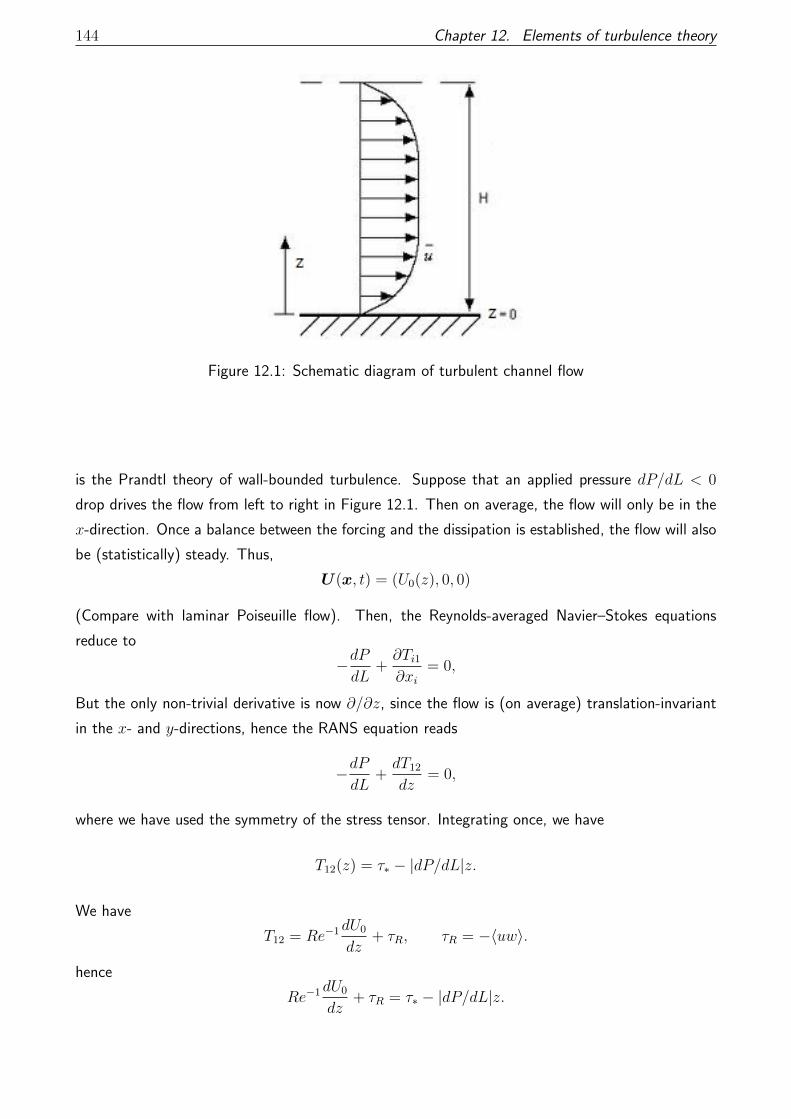
144 Chapter 12. Elements of turbulence theory
Figure 12.1: Schematic diagram of turbulent channel flow
is the Prandtl theory of wall-bounded turbulence. Suppose that an applied pressure dP/dL < 0
drop drives the flow from left to right in Figure 12.1. Then on average, the flow will only be in the
x-direction. Once a balance between the forcing and the dissipation is established, the flow will also
be (statistically) steady. Thus,
U(x, t) = (U0(z), 0, 0)
(Compare with laminar Poiseuille flow). Then, the Reynolds-averaged Navier–Stokes equations
reduce to
−dPdL
+∂Ti1∂xi
= 0,
But the only non-trivial derivative is now ∂/∂z, since the flow is (on average) translation-invariant
in the x- and y-directions, hence the RANS equation reads
−dPdL
+dT12
dz= 0,
where we have used the symmetry of the stress tensor. Integrating once, we have
T12(z) = τ∗ − |dP/dL|z.
We have
T12 = Re−1dU0
dz+ τR, τR = −〈uw〉.
hence
Re−1dU0
dz+ τR = τ∗ − |dP/dL|z.

12.4. Eddy-viscosity model for channel flows 145
where τ∗ is the wall shear stress, to be determined. Using the mixing-length theory, we obtain
τR = κ2
∣∣∣∣dU0
dz
∣∣∣∣ z,and thus the RANS balance equation reads
Re−1dU0
dz+ κ2z2dU0
dz
∣∣∣∣dU0
dz
∣∣∣∣ = τ∗ − |dP/dL|z.
This equation contains a lot more information than is apparent superficially. We identify a viscous
sublayer where the viscous stress dominates over the Reynolds stress, which will exist for z → 0,
wherein the dominant balance reads
ρνdU0
dz∼ τ∗ := ρu2
∗,
hence
νdU0
dz∼ u2
∗
where we have momentarily restored the dimensional variables. The typical velocity scale in this
zone is u∗ and the typical lengthscale is the friction scale d∗, giving
νu∗d∗∼ u2
∗,
hence d∗ = ν/u∗, where the friction velocity u∗ is to be determined. The range 0 ≤ z > d∗ is
therefore called the viscous sublayer of the flow. We next identify a region d∗ z H/2 where
the dominant balance in the RANS equation reads
ρκ2z2dU0
dz
∣∣∣∣dU0
dz
∣∣∣∣ ∼ τ∗ = ρu2∗
hence
κzdU0
dz∼ u∗,
where we have assumed that we are near the bottom wall, such that dU0/dz > 0 (the same
arguments will apply near the top wall, by symmetry around the channel centreline). Integration
now gives
U0 ∼u∗κ
log z + Const.
which is the famous law of the wall of turbulence theory.
It would be useful to find an expression for the friction velocity in terms of the problem parameters,
and at the same time, to solve for the velocity profile U0(z) throughout the entire domain 0 ≤ z ≤ H.
This is done now here a very simple eddy-viscosity model. However, before presenting this model, it

146 Chapter 12. Elements of turbulence theory
is useful to understand the scaling of the Reynolds stress (and hence the base-state velocity profile)
near the wall at z = 0. We therefore Taylor-expand the velocity fluctuations near the bottom wall:
u(x, y, z, t) = a0(x, y, t) + a1(x, y, t)z + a2(x, y, t)z2 + · · ·
v(x, y, z, t) = b0(x, y, t) + b1(x, y, t)z + b2(x, y, t)z2 + · · ·
w(x, y, z, t) = c0(x, y, t) + c1(x, y, t)z + c2(x, y, t)z2 + · · ·
The no-slip condition obviously gives a0 = b0 = c0, hence
u(x, y, z, t) = a1(x, y, t)z + a2(x, y, t)z2 + · · ·
v(x, y, z, t) = b1(x, y, t)z + b2(x, y, t)z2 + · · ·
w(x, y, z, t) = c1(x, y, t)z + c2(x, y, t)z2 + · · ·
The same condition gives∂w
∂x=∂w
∂y=∂v
∂x=∂v
∂y=∂u
∂x=∂u
∂y
at z = 0 and hence, by incompressibility,
∂w
∂z= 0
at z = 0. Therefore, c1 = 0 identically, and hence,
uw =(a1(x, y, t)z + a2(x, y, t)z2 + · · ·
) (c2(x, y, t)z2 + · · ·
),
= a1c2z3 + · · · ,
hence
τR = −〈uw〉 = −〈a1c2〉z3 +O(z4),
as z → 0.
12.4.1 The model
Instead of starting from the mixing-length theory, we start from scratch, and derive the eddy viscosity
using an alternative approach. We first of all introduce from first principles the non-dimensionaliztion
scheme for the RANS balance equation. Thus, we introduce a velocity scale
Up =√|dP/dL|h/ρ

12.4. Eddy-viscosity model for channel flows 147
and the Reynolds number
Rep = ρUph/µ
The problem contains a further, apparently unknown parameter, Re∗, based on the friction velocity:
Re∗ =ρU∗h
µ, ρU2
∗ = µdU0
dz
∣∣∣∣z=0
.
which will be determined by the model. These considerations therefore suggest the following func-
tional form for the (dimensionless) eddy viscosity:
µT (z) = Re∗F (z/h)
where henceforth we use z for z/h. We are therefore dealing with an algebraic closure model.
We make the inspired guess
F = κψw(z)ψw(1− z)G(z),
where
G(z) = z(1− z)
[1− 3z(1− z)
1− z(1− z)
], (12.3)
and where
ψw(z) = 1− e−αz2Re2∗ ,
is a wall function (See References [Bib07, NSMZ11]). The parameter α is fixed such that
U(z = 5d∗) = 0.95(u2∗z/ν)z=5d∗ = 0.95× 5u∗.
Thus, the velocity is obtained through the relation
U(z) =Re2∗
Re0
∫ z
0
(1− Re20
Re2∗s)
ds
1 + κRe∗G(s)ψw(s)ψw(1− s)(12.4)
The friction velocity is thus obtained through the following root-finding condition for Re∗:
U(z = 1;Re∗) = 0.
The clever thing about the choice (12.3) for the algebraic closure is that the correct scaling is
recovered for U(z) in the log layer and in the viscous sublayer. Also, the model is symmetric around
the centreline, with G(z) = G(1− z).
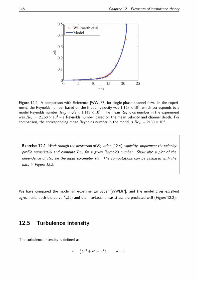
148 Chapter 12. Elements of turbulence theory
Figure 12.2: A comparison with Reference [WWL87] for single-phase channel flow. In the experi-ment, the Reynolds number based on the friction velocity was 1.143× 10³, which corresponds to amodel Reynolds number Rep =
√2× 1.143× 103. The mean Reynolds number in the experiment
was Rem = 2.158× 10⁴ – a Reynolds number based on the mean velocity and channel depth. Forcomparison, the corresponding mean Reynolds number in the model is Rem = 2130× 104.
Exercise 12.1 Work though the derivation of Equation (12.4) explicitly. Implement the velocity
profile numerically and compute Re∗ for a given Reynolds number. Show also a plot of the
dependence of Re∗ on the input parameter Re. The computations can be validated with the
data in Figure 12.2.
We have compared the model an experimental paper [WWL87], and the model gives excellent
agreement: both the curve U0(z) and the interfacial shear stress are predicted well (Figure 12.2).
12.5 Turbulence intensity
The turbulence intensity is defined as
k = 12〈u2 + v2 + w2〉, ρ = 1.

12.5. Turbulence intensity 149
We derive a transport equation for the turbulent kinetic energy, writing the Navier–Stokes equations
in the following decomposition:
∂
∂t(〈U〉+ u) + (〈U〉+ u) · ∇ (〈U〉+ u) = −∇〈p〉 − ∇p′ + 1
Re∇2〈U〉+
1
Re∇2u.
But we also have the RANS equation
∂
∂t〈U〉+ 〈U〉 · ∇〈U〉 = −∇〈p〉+
1
Re∇2〈U〉+∇ · τ .
Subtract these equations and take components to obtain[∂
∂t+ (〈U〉+ u) · ∇
]ui = −uj
∂
∂xj〈Ui〉+
∂
∂xj〈uiuj〉 −
∂p′
∂xi+
1
Re∇2ui.
Multiply both sides by ui, sum over i and average. On the LHS we obtain⟨ui
[∂
∂t+ (〈U〉+ u) · ∇
]ui
⟩=
∂k
∂t+ 〈Uj〉
⟨ui∂ui∂xj
⟩+
⟨uiuj
∂ui∂xj
⟩,
=∂k
∂t+ 〈U〉 · ∇k +
⟨uiuj
∂ui∂xj
⟩,
=∂k
∂t+ 〈U〉 · ∇k + 1
2
∂
∂xj〈|u|2uj〉.
where we have used ⟨uiuj
∂ui∂xj
⟩=
⟨ui
∂
∂xj(uiuj)
⟩= 1
2
∂
∂xj〈uiuiuj〉,
On the right-hand side, we work on each term individually. We identify the production of turbulent
kinetic energy:
P = −〈uiuj〉∂
∂xj〈Ui〉 = τ : ∇〈U〉.
Also, ⟨ui∂p′
∂xi
⟩=
∂
∂xi〈uip′〉.
Finally, the term 〈ui∇2ui〉 is re-arranged as
〈ui∇2ui〉 =∂
∂xj
⟨ui∂ui∂xj
⟩−⟨∂ui∂xj
∂ui∂xj
⟩.
We identify the dissipation of turbulent intensity:
ε := − 1
Re
⟨∂ui∂xj
∂ui∂xj
⟩≤ 0.
150 Chapter 12. Elements of turbulence theory
Thus, the equation for the turbulent kinetic energy reads(∂
∂t+ 〈U〉 · ∇
)k +∇ ·R = P − ε, (12.5)
where the vector R represents redistribution of turbulent intensity:
Ri = 12〈|u|2ui〉+ 〈uip′〉 −
1
Re
⟨uj∂uj∂xi
⟩.
These results give great insight into the energy budget that underlies turbulence generation: it is
the interaction between the Reynolds stresses and the mean flow that generates turbulence via the
production term τ : ∇〈U〉, while the turbulence is dissipated via molecular dissipation.
Exercise 12.2 Show that Equation (12.5) can be rewritten in the following (equivalent) way:(∂
∂t+ 〈U〉 · ∇
)k +∇ ·R′ = P − ε′, (12.6)
where the meaning of P is unchanged, but where
R′i = 12〈|u|2ui〉+ 〈uip′〉 − (2/Re)〈ujsij〉,
and
ε′ = (2/Re)〈sijsij〉.
Also, sij is the rate-of-strain tensor associated with the fluctuating velocities,
sij = 12
(∂ui∂xj
+∂uj∂xi
).
We now use this theory to prove an important result:
Theorem 12.1 For homogeneous turbulence, the most general form for the mean velocity profile
is
〈Ui〉 = ai(t) + bij(t)xj
Recall, the definition of homogeneous turbulence means that the statistics of the turbulent velocity
fluctuations are translation invariant. Thus, for homogeneous turbulence, we have
k = 12〈|u|2〉, Ri = 1
2〈|u|2ui〉+ 〈uip′〉 −
⟨ui∂ui∂xj
⟩, ε = − 1
Re
⟨∂ui∂xj
∂ui∂xj
⟩,

12.6. K-41 theory 151
Figure 12.3: Schematic description of the different lengthscales involved in turbulence
all independent of space. We substitute these results into the turbulent kinetic energy equation to
obtain∂k
∂t+ ε = P
and it follows that the production is independent of spatial coordinates, i.e.
−〈uiuj〉∂
∂xj〈Ui〉
is independent of space. But −〈uiuj〉 is independent of space also, and so (∂/∂xi)〈Uj〉 is indepen-
dent of space. It therefore follows that
〈Ui〉 = ai(t) + bij(t)xj,
such that (∂/∂xi)〈Uj〉 = bij(t), independent of space, as required.
Having now understood something of the mechanisms underlying the production, transport, and
dissipation of turbulence intensity, we can now study a more detailed (but phenomenological) theory
for these processes, which underscores the multiscale nature of these turbulence mechanisms.
12.6 K-41 theory
The idea of the Kolmogorov-1941 (K-41) theory is to break up the motion into three ranges (Fig-
ure 12.3 ).

152 Chapter 12. Elements of turbulence theory
Energy-containing range
On these scales, the motion is made up of large-scale coherent motions called ‘eddies’. A typical
eddy in this range is of size `0, with `0 ∼ L, where L is the lengthscale of the domain. The
characteristic velocity of the eddies will be u0 = u(`0), with u0 = [(2/3)k]1/2, where k is the
turbulence intensity, which in turn is comparable to U , the typical flow magnitude on the domain
scale. We have Re0 = u0`0/ν, which is the Reynolds number associated with the large eddy. Also,
Re0 ∼ Re, where Re = UL/ν, which is the Reynolds number associated with the domain scales.
The large eddies interact with the smaller eddies via the nonlinear term in the NS equation, leading
to a transfer of energy from the larger eddies to the smaller ones. This process continues (in three
dimensions) down to the smallest scales where dissipation dominates over inertia in the Navier–
Stokes equation, such that energy is eventually dissipated from the system.
The large eddies have an energy of order u20 and a timescale τ0 = `0/ν0, so the rate of transfer
of energy can be supposed to scale as u20/τ0 = u3
0/`0. Because the dissipation is controlled by
the transfer, it can also be supposed that the dissipation rate ε scales as u30/`0, independent
(shockingly) of ν!!
Inertial and dissipation ranges
In the inertial range and the dissipation range, Kolmogorov’s similarity hypotheses are assumed to
hold:
• At sufficiently high Reynolds number, the small-scale turbulent motions (` `0) are statisti-
cally isotropic.
• In every turbulent flow a t sufficiently high Reynolds number, the statistics of the small-scale
motions (` < `EI) have a universal form that is uniquely determined by ν and ε.
In the dissipation range, dimensional analysis gives
η = (ν3/ε)1/4 · · · lengthscale
uη = (εν)1/4 · · · velocity scale
τη = (ν/ε)1/2 · · · time scale.
Note that
Reη = 1,

12.6. K-41 theory 153
meaning that dissipation is important (not surprisingly!) in the dissipation range. The ratio of the
smallest to largest scales is thus given by
η
`0
=ν3/4
`0ε1/4,
=ν3/4
`0(u30/`0)1/4
,
=ν3/4
u3/40 `
1−(1/4)0
,
= (ν/u0`0)−3/4,
∼ Re−3/4,
hence η/`0 ∼ Re−3/4. Similarly,
uη/u0 ∼ Re−1/4, τη/τ0 ∼ Re−1/2.
Thus, at very high Reynolds numbers, the scales of motion (length, velocity and time) are all much
smaller in the small eddies in the dissipative range than in the larger eddies in the energy-containing
range.
Crucially for direct numerical simulation of turbulence, the numerical simulation must resolve down
to the dissipative scales, such that
∆x ≤ η,
hence
∆x/`0 ≤ (η/`0) ∼ Re−3/4.
The number of gridpoints in the problem is N = (`0/∆x)3 for a full three-dimensional simulation
and hence,
N ∼ Re9/4
is the number of grid points required in a three-dimensional direct numerical simulation of turbulence.
A further consequence of the formula η/`0 ∼ Re−3/4 is the obvious fact that η `0 at high
Reynolds numbers, meaning that there is a range of lengthscales `, with
η ``0
which correspond neither to the dissipative range nor the energy-containing range. This is the
inertial range. Again, in this range, it is expected that the Kolmogorov hypotheses should hold,
giving
u(`) = (ε`)1/3 = ε1/3`1/3.

154 Chapter 12. Elements of turbulence theory
But
uηη1/3 =
(εν)1/4
[(ν3/ε)1/4]1/3,
=
[(εν)3/4
(ν3/ε)1/4
]1/3
,
=
[ε3/4ν3/4ε1/4
ν3/4
]1/3
,
= ε1/3,
hence
u(`) = uη(`/η)1/3.
We have
uη(`/η)1/3 = u0(uη/u0)(`0/`η)1/3(`/`0)1/3,
= u0(`/`0)1/3(uη/u0)(`0/`η)1/3,
= u0(`/`0)1/3Re−1/4Re1/4,
= u0(`/`0)1/3,
hence u(`) ∼ u0(`/`0)1/3. Similarly,
u(`) ∼ u0(`/`0)1/3, τ(`) ∼ τ0(`/`0)2/3, (12.7)
such that, in the inertial range, the velocity scales u(`) and timescales τ(`) decrease as ` decreases.
The energy cascade
The rate at which energy is transferred from a scale ` to (smaller) scales is denoted by T (`) and is
expected to scale as
T (`) ∼ u(`)2/τ(`).
By Equation (12.7), we have
T (`) ∼ u20`
2/3`−2/30
τ0`2/3`−2/30
=u2
0
τ0
= ε,
and thus, the transfer rate is independent of the scale: the transfer rate is the same on all
lengthscales.
12.6. K-41 theory 155
The energy spectrum
The energy spectrum is introduced as follows, starting with the total turbulent kinetic energy:
E =
∫d3x
(12|u|2
),
= 12
∫d3k
(2π)3|uk|2,
=
∫ ∞0
dk
(12k2
∫Ω
dΩ |uk|2),
:=
∫ ∞0
dk E(k),
and E(k) is called the energy spectrum.
In the inertial range, by Kolmogrovo’s similarity hypotheses, the energy spectrum is determiend
entirely by ε and ν: we have
E(k) = εaνbkc,
and dimensional analysis gives
2a+ 3b− c = 3,
3a+ b = 2.
The system of equations is underdetermined. However, in the inertial range, the viscosity does not
have a direct effect on the eddies. This can be seen as follows:
Re(`) =u0(`/`0)1/3`
ν,
=u0`0
ν(`/`0)1/3(`/`0),
= Re0(`/`0)4/3 1,
with Re(`) = 1 at the onset of th dissipation range. This direct viscous effects are negligible in the
inertial range, and we therefore take b = 0, hence a = 2/3 and c = −5/3, giving
E(k) = Cε2/3k−5/3,
which is the celebrated Kolmogorov spectrum of turbulence.
The Kolmogorov spectrum is a fairly well-established feature of three-dimnensional turbulence (e.g.
Figure 12.4). To understand this figure fully, consider for definiteness a channel flow with walls
bounding the flow in the z direction, with (x, y, z) ∈ [0, Lx]× [0, Ly]× [0, H]. One starts with the

156 Chapter 12. Elements of turbulence theory
Figure 12.4: Experimental validation of the Kolmogorov spectrum in the inertial range for a variety ofdifferent turbulent flows, taken from Reference [Pop00]. As the statistics of turbulence are universalin the inertial and dissipative ranges, it is expected that the Kolmogorov spectrum will hold, notmatter what are the details of the large-scale geometry and forcing.

12.6. K-41 theory 157
following two-point correlation function in real space:
Rij(x, y, z) =1
t2 − t11
LxLy
∫ t2
t1
dt
∫ Lx
0
dx′∫ Ly
0
dy′Ui(x+x′, y+y′, z)Uj(x′, y′, z)−〈Ui〉(z)〈Uj〉(z);
(12.8)
Then, based on Equation (12.8), one takes a Fourier transform in plane parallel to the walls at
location z, defined as follows:
Rij(kx, ky, z) =x
[0,Lx]×[0,Ly ]
dxdy e−ikxx−ikyyRij(x, y, z).
The vertical axis in Figure 12.4 shows E11(kx, z) := |Rij(kx, 0, z)|. For a channel flow, this would be
typically taken at the channel midpoint z = H/2. Because turbulence is homogeneous and isotropic
at sufficiently small scales, it shouldn’t matter that we are looking at a Fourier transform involving
only the kx-wavenumbers. Also, it shouldn’t matter that we are looking at the correlation function
in the particular directions i = j = 1. Thus, it is expected that the famous Kolmogorov scaling law
E11(kx) ∼ k−5/3x should apply, as indeed it does in Figure 12.4 – in the window where the spectrum
exhibits the straight-line behaviour on the loglog scale – to a wide range of different experiments at
different (sufficiently high) Reynolds numbers. For sufficiently small scales, and across the range of
experiments on show, the spectrum exhibits exponential decay (or possibly faster-than-exponential
decay), corresponding to the dissipation range.
The Kolmogorov scaling theory is also self-consistent, in the following sense. For, taking E(k) =
Ak−p, the energy contained in a wavenumber range k ∈ (k0,∞) is
Energy[k ∈ (k0,∞)] =
∫ ∞k0
E(k)dk =A
p− 1k−(p−1)0 ,
meaning that p > 1 for a finite energy. Also, the total dissipation can be expressed as
ε = 2ν
∫d3x sijsij, sij = 1
2
(∂ui∂xj
+∂uj∂xi
)where Sij is the instantaneous rate-of-strain tensor. Using Parseval’s identity, this is
ε = 2ν
∫ ∞0
dk k2E(k),
and the amount of dissipation occuring in the scales k ∈ (0, k0) is thus
Dissipation[k ∈ (0, k0)] = 2ν
∫ k0
0
dkm2E(k) =2νA
3− pk3−p
0 .
Therefore, in order for the dissipation in the scales (0, k0) to remain finite as k0 → 0, we need

158 Chapter 12. Elements of turbulence theory
p < 3. Thus, we need 1 < p < 3, and the K-41 theory is definitely consistent with this requirement.
Indeed, with the K-41 theory, we have
Energy[k ∈ (k0,∞)] ∼ k−2/30 ,
which properly deceases as one goes to larger k0 (smaller lengthscales), and
Dissipation[k ∈ (0, k0)] ∼ k4/30 ,
which also properly decreases as one goes to smaller k0 (larger lengthscales).
The second-order structure function
We introduce the following two-point correlation called the structure function:
Dij(r,x, t) = 〈[Ui(x+ r, t)− Ui(x, t)] [Uj(x+ r, t)− Uj(x, t)]〉.
For homogeneous turbulence, we have
Dij(r,x, t) = Dij(r, t)
only, and we therefore have the following fact:
Theorem 12.2 For the second-order structure function in homogeneous turbulence, we have
∂Dij(r, t)
∂ri= 0.
Proof: We have
Dij(r, t) = 〈Ui(x+r, t)Uj(x+r, t)〉−〈Ui(x+r, t)Uj(x, t)〉−〈Ui(x, t)Uj(x+r, t)〉+〈Ui(x, t)Uj(x, t)〉.
Hence,
∂Dij(r, t)
∂ri=
⟨[∂
∂riUi(x+ r, t)
]Uj(x+ r, t)
⟩+
⟨Ui(x+ r, t)
[∂
∂riUj(x+ r, t)
]⟩−⟨[
∂
∂riUi(x+ r, t)
]Uj(x, t)
⟩−⟨Ui(x, t)
[∂
∂riUj(x+ r, t)
]⟩

12.6. K-41 theory 159
A few of these terms are obviously zero because of incompressibility, and we are left with
∂Dij(r, t)
∂ri=
⟨Ui(x+ r, t)
[∂
∂riUj(x+ r, t)
]⟩−⟨Ui(x, t)
[∂
∂riUj(x+ r, t)
]⟩=
⟨[Ui(x+ r, t)− Ui(x, t)]
[∂
∂riUj(x+ r, t)
]⟩We break up these terms into the fluctuating component and the mean component, remembering
that
〈Ui〉 = ai(t) + bij(t)rj
for homogeneous turbulence. Thus,
Ui(x+ r, t)− Ui(x, t) = [ui(x+ r, t)− ui(x, t)] + bikrk,
∂
∂riUj(x+ r, t) =
∂
∂riuj(x+ r, t) + bimxm
Hence,
∂Dij(r, t)
∂ri=
⟨[(ui(x+ r, t)− ui(x, t)) + bikrk]
[∂
∂riuj(x+ r, t) + bij
]⟩,
=
⟨[(ui(x+ r, t)− ui(x, t))]
[∂
∂riuj(x+ r, t)
]⟩+ 〈[(ui(x+ r, t)− ui(x, t))] bij〉
+
⟨bikrk
[∂
∂riuj(x+ r, t)
]⟩+ 〈bikbijrk〉.
Hence,
∂Dij(r, t)
∂ri=
⟨rk
[∂
∂xkui(x)
] [∂
∂riuj(x+ r, t)
]⟩+1
2
⟨rkrm
[∂2
∂xkxmui(x)
] [∂
∂riuj(x+ r, t)
]⟩+· · ·
+
⟨rk
[∂
∂xkui(x)
]bij
⟩+ 1
2
⟨rkrm
[∂2
∂xkxmui(x)
]bij
⟩+
⟨bikrk
[∂
∂riuj(x+ r, t)
]⟩+ 〈bikbijrk〉.
and these correlations now involve only the (homogeneous) fluctuations and are therefore indepen-
dent of r. We can therefore set r = 0 everywhere, giving
∂Dij(r, t)
∂ri= 0.
We now return to the structure function Dij(r, t) for homogeneous isotropic turbulence. Now,
the only second-order homogeneous isotropic tensors that can be formed from the vector r are δij
160 Chapter 12. Elements of turbulence theory
and rirj, hence
Dij(r, t) = DNN(r, t)δij + [DLL(r, t)−DNN(r, t)]rirjr2
.
Using ∂iDij(r, t) = 0, we obtain
DNN(r, t) = DLL(r, t) + 12r∂
∂rDLL (12.9)
Exercise 12.3 Prove Equation (12.9).
Now, it follows from the Kolmogorov similarity hypotheses that any kind of turbulence is homo-
geneous and isotropic on the small scales, and thus the previous arguments will apply to any kind
of turbulence for r sufficiently small. Therefore, in the inertial range and below, for any kind of
turbulence, and using the second similarity hypothesis, we have
DLL(r, t) = (εr)2/3DLL(r/η).
where DLL is a dimensionless universal function. In the inertial range, where the effects of the
viscosity are only indirect, we will have
DLL(r, t) = C(εr)2/3,
where C is a universal constant. Using Equation (12.9) above, we will also have DNN = (4/3)DLL
and hence, in the inertial range,
Dij = C2(εr)2/3(
43δij − 1
3
rirjr2
).
12.7 Direct numerical simulation (DNS)
As the name would suggest, the full three dimensional and time dependent Navier–Stokes equations
are solved on a computational mesh which is fine enough to resolve the smallest length scale eddies
present in the flow, and for a domain which is large enough to allow the largest eddies to develop.
The main drawback of this method is its associated computational cost, and it cannot be applied
to large Reynolds number flows which are of interest (e.g. for the flow about an airplane with a
characteristic velocity of 30 m/s, the Reynolds number is typically 2×10⁷ requiring in excess of 1017
grid points). However, due to the resolution used, they provide the most accurate computational
results attainable, which can then be compared to direct experimental results in certain cases

12.8. Large-eddy simulation 161
12.8 Large-eddy simulation
With thanks to James Fannon who provided text for this section.
LES can be thought of as a middle road in terms of complexity between RANS and DNS. Main idea
behind an LES is to obtain a so-called filtered velocity u by forming a convolution between the full
velocity field and a given homogeneous (i.e. space independent) filter function G (r) such that:
u (x, t) =
∫Ω
G (r)u (x− r, t) dnx (12.10)
where the integral is taken over the domain Ω. Typical examples of such filter functions are the box
filter:
G(r) =
1L, |r| ≤ L
2
0, |r| > L2
and Gaussian filter:
G(r) =1√πL
exp
(−r2
L2
)which allow for local averages of u (x, t) in the neighbourhood of x to be computed, where the
average is taken over a length scale L [Dav09]. The effect of this process is to allow for the
larger, energy carrying eddies to be resolved exactly while filtering out the small-scale eddies (Fig-
ure 12.5). Although these eddies are not simulated directly, their effect on the rest of the flow
is modelled [Dav09]. As such, a LES is more accurate than a RANS simulation as the unsteady
large-scale eddies are computed exactly, while it is not as computationally expensive as a full DNS
as the smaller scales are not resolved. Thus, it provides a very useful middle ground between both
methods. According to Reference [Pop00], the four main steps involved in a LES are given by:
1. A filtering operation is applied to the full velocity field in order to form the filtered velocity
u (x, t), which describes the motion of large-scale eddies, and the fluctuating velocity field
u′ (x, t) which describes the motion of the smaller, unresolved eddies.
2. Obtain the governing equations for u (x, t) from the NSE. These contain an additional term
known as the residual stress tensor.
3. The residual stress tensor is modelled in such a way that it takes into account the effect of
the unresolved eddies on the rest of the flow. Hence closure is obtained.
4. The governing equations, which are now closed, are then solved numerically. This allows for
the large-scale eddies in the flow to be computed exactly.
We now place our focus on deriving the governing equations for u (x, t), for a general form of the
filtered velocity as defined by equation 12.10. Let us apply the filtering process to the dimensionless

162 Chapter 12. Elements of turbulence theory
Figure 12.5: Application of a filtering process to the full velocity field ux yields a filtered velocity uLxwhich accurately represents the large-scale features but removes the small-scale fluctuations [Dav09].
NSE. We apply the filtering operation (as defined by equation 12.10) to these equations and use the
fact that the operations of filtering (denoted by the barred variables) and differentiation commute
(Technically, this is only true for homogeneous filters [Pop00]), i.e.:
(∂ui∂t
)=∂ui∂t,
(∂ui∂xj
)=∂ui∂xj
and similarly for the pressure. Hence one obtains:
∂ui∂t
+∂
∂xj(uiuj) = − ∂p
∂xi+
1
Re∗
∂2ui∂xj∂xj
∂ui∂xi
= 0
By rewriting the first equation and using the incompressibility condition, we arrive at the filtered
equations of motion [San09]:
∂ui∂t
+ uj∂ui∂xj
= − ∂p
∂xi+
1
Re∗
∂2ui∂xj∂xj
− ∂τij∂xj
(12.11)
∂ui∂xi
= 0 (12.12)
where we define the residual stress tensor as:
τij = uiuj − ui uj (12.13)
Note that these equations are analogous to the RANS equations derived previously, but the interpre-
tation of what the variables signify is very different. In the RANS equations, ui represents the mean
flow, while in the filtered equations of motion, the variable ui represents the motion of large-scale
eddies and hence can be thought of as the mean flow plus the large-scale turbulent motion [Dav09].

12.9. LES method – implementation 163
As the residual stress term contains the unknown variable ui, it remains to formulate an appropriate
method of modelling this term so to achieve closure of the system.
Over the past 40 years, LES have proved to be an invaluable tool for researchers interested in
studying turbulent flow. The method was first implemented in Reference [Dea70] who, despite
using a resolution of only 6720 grid points, obtained some promising results, and paved the way for
a number of future researchers e.g. Reference [Sch75] and Reference [Pio93]. Despite the positive
aspects of LES, its main weakness, as stated in the critical review carried out in Reference [Mas94],
occurs at near surface regions where the turbulent length scales become small in relation to the filter
width (the filter width associated with a LES is the cut-off length scale beyond which no eddies
are resolved). Here, a much finer computational mesh would be needed to take into account the
effect of these small-scale eddies. Ideally, one would use an adaptive grid when solving the NSE
computationally, where the grid spacing itself is a function of position. In such a scheme, a higher
resolution would be used close to surfaces than would be used in the rest of the domain.
12.9 LES method – implementation
The filter function G (r) as discussed in section 12.8 is incorporated implicitly into a numerical
simulation by means of the resolution of the computational mesh itself i.e. the grid spacing provides
a natural filter for defining the smallest length scale eddies resolvable in the simulation. As such, it
remains to model the residual stress term (also known as the Subgrid-Scale (SGS) term):
τij = uiuj − ui uj
In a turbulent flow, the net transfer of energy from large to small eddies appears as an energy loss or
dissipation from the large-scale eddies. As such, the primary function of the SGS term is to remove
energy from the resolved eddies at an appropriate rate, and thus the proposed model for it should
be dissipative in nature [AB97]. The most common method of modelling this term is that proposed
by [Sma63], known as the eddy-viscosity model:
τij = −2νtsij
where νt is the so-called eddy viscosity, while the rate of strain tensor with respect to the filtered
velocity is given by:
sij =1
2
(∂ui∂xj
+∂uj∂xi
)The eddy viscosity should be determined by the most energetic of the unresolved eddies in the simu-
lation [Dav09]. As such, let ∆ denote the characteristic length scale of the largest, and hence most

164 Chapter 12. Elements of turbulence theory
energetic, unresolved eddies. According to [Dea70], this length scale is proportional to (∆x∆y∆z),
and here we take the value as quoted by [AB97]:
∆ = 2 (∆x∆y∆z)1/3 (12.14)
On dimensional grounds, one knows that [νt] = [Length]2/Time, and thus a natural proposition for
νt is of the form:
νt ∼ ∆ (v∆)
where v∆ is a velocity scale for eddies of size ∆. [Sma63] took this velocity scale to be:
v∆ = ∆ |s| , where |s| =√
2 (sij) (sij)
As such, the eddy viscosity term becomes:
Figure 12.6: Plot of φw (z) for p = q = 1, A = 25 and Re∗ = 360, the Reynolds number used inthe LES.
νt = C2S∆2 |s| (12.15)
where CS is a dimensionless constant known as the Smagorinsky coefficient, usually taken to be
CS = 0.1 [Dav09]. Furthermore, in order to take into account the turbulence near the walls
z = 0, 1, where the largest unresolved eddies decrease in size, we use the method of near wall
modelling (NWM). This method amounts to introducing a wall damping function φw (z), which is
12.9. LES method – implementation 165
given by [San09]:
φw (z) =
(1− exp
[(−zRe∗A
)]p)q, z ≤ 1
2(1− exp
[−(1−z)Re∗
A
]p)q, z ≥ 1
2
(12.16)
as an additional prefactor for the length scale ∆. In this LES, we take the values p = q = 1 and
A = 25, in keeping with the standard Van Driest components. A plot of the wall damping function
for the parameters of interest is given in figure 12.6. The use of this function is both simple to
implement numerically and saves computational cost, as compared to introducing a finer mesh grid
at the wall which would provide a much more accurate means of modelling the turbulence there.
As such, by incorporating the wall damping function, the eddy viscosity term to be implemented
numerically is given by:
νt = (CS∆φw)2 |s| (12.17)
Now substituting the model for the SGS term:
τij = −νt(∂ui∂xj
+∂uj∂xi
)(12.18)
into Equation (12.11), we find that:
∂ui∂t
+ uj∂ui∂xj
= − ∂p
∂xi+
1
Re∗
∂2ui∂xj∂xj
− ∂
∂xj
(−νt
(∂ui∂xj
+∂uj∂xi
))which can be rewritten as:
∂ui∂t
+ uj∂ui∂xj
= − ∂p
∂xi+
∂
∂xj
((1
Re∗+ νt
)(∂ui∂xj
+∂uj∂xi
))again using the incompressibility condition.
12.9.1 Initialization
The turbulence initialization technique which will be implemented in this study is that presented
by [BGC04] and [BBP08]. A summary of the method and its numerical implementation will be
presented below. First, the initial velocity field to be constructed (u (x)) is written as a vector
potential:
u(x) = ∇× (A (x) f (z)) (12.19)

166 Chapter 12. Elements of turbulence theory
where the function f (z) is an appropriate scaling function of the vector field A (x) which ensures
that the no-slip boundary conditions at z = 0, 1 are enforced. Expanding Equation (12.19) we have:
u = f (z) (∇×A (x)) + (∇f)×A (x)
=⇒ u = f (z)
∣∣∣∣∣∣∣∣x y z
∂x ∂y ∂z
Ax Ay Az
∣∣∣∣∣∣∣∣+
∣∣∣∣∣∣∣∣x y z
0 0 fz
Ax Ay Az
∣∣∣∣∣∣∣∣and hence each component of u(x) is given by:
u = f (z) (∂yAz − ∂zAy)− Aydf
dz(12.20)
v = f (z) (∂zAx − ∂xAz) + Axdf
dz(12.21)
w = f (z) (∂xAy − ∂yAx) (12.22)
As such, in order to ensure that each component vanishes at z = 0, 1 we use the following form for
the scaling function:
f (z) =1
2+
1
2sin
(2πz
Lz− π
2
)=⇒ df
dz=
π
Lzcos
(2πz
Lz− π
2
)(12.23)
where Lz = 1 is included explicitly for completeness. It now remains to define the velocity field
A (x). There are a number of features which we want this field to have:
1. As we wish to initialize the system with a turbulent velocity field, the fieldA should incorporate
some randomness.
2. It must satisfy the periodic boundary conditions in the streamwise and spanwise directions.
This suggests that we take a Fourier sum for each component of the field (where i = x, y, z):
Ai (x) =
Ckx∑kx=1
Cky∑ky=1
Ckz∑kz=1
[Si (kx, ky, kz) sin (k · x) + Ci (kx, ky, kz) cos (k · x)] (12.24)
where we have a sum over the wavenumber k:
k =
(2π
Lxkx,
2π
Lyky,
2π
Lzkz
)and the constants Si (kx, ky, kz) and Ci (kx, ky, kz) are random numbers between 0 and 1.

12.10. TPLS 167
12.10 TPLS
TPLS stands for Two-phase Levelset, and is a code created by the present author (along with
Dr Prashant Valluri, University of Edinburgh), for simulating two-phase flows. This code solves
the Navier–Stokes equations for two fluids, simulating the interface between the two phases using
a levelset formulation. The code, written in Fortran 90, is fully parallelized using the MPI and
OpenMP parallelisation schemes, so that it can be run on thousands of CPU cores, and has been
rigorously validated. A single-phase version also exists and is capable of simulating turbulence using
LES with the Smagorinsky model above – see
https://sourceforge.net/p/tpls/code/HEAD/tree/trunk/s-tpls/
Exercise 12.4 Obtain the single-phase turbulent version of TPLS. Configure and compile a
version on whatever multicore machine you can find. Run the code for a sufficient length of
time to generate turbulent statistics. Plot the average streamwise turbulent velocity field.

Appendix A
M codes
A numerical method for solving the model diffusion problem is implemented below.
1 f u n c t i o n [ xx , yy , C , t i m e v e c , norm decay ]= t e s t d i f f u s i o n j a c o b i ( )
2
3 % Numer i ca l method to s o l v e
4 % ( d/ dt )C=[D xx+D yy ]C+s ( x , y ) ,
5 % s u b j e c t to p e r i o d i c boundary c o n d i t i o n s i n the x−d i r e c t i o n ,
6 % and Neuman boundary c o n d i t i o n s at y=0 and y=L y .
7
8 % ∗∗∗∗∗∗∗∗∗∗∗∗∗∗∗∗∗∗∗∗∗∗∗∗∗∗∗∗∗∗∗∗∗∗∗∗∗∗∗∗∗∗∗∗∗∗∗∗∗∗∗∗∗∗∗∗∗∗∗∗∗∗∗∗∗∗∗∗∗∗∗∗∗9 % S i m u l a t i o n p a r a m e t e r s
10
11 [ Nx , Ny , ˜ , ˜ , A0 , dx , dy , kx0 , ky0 , dt , ˜ , n t i m e s t e p s ]= f i x a l l p a r a m e t e r s ( ) ;
12
13 % m a x i t e r a t i o n f o r d i f f u s i o n :
14 m a x i t e r a t i o n =30;
15
16 % ∗∗∗∗∗∗∗∗∗∗∗∗∗∗∗∗∗∗∗∗∗∗∗∗∗∗∗∗∗∗∗∗∗∗∗∗∗∗∗∗∗∗∗∗∗∗∗∗∗∗∗∗∗∗∗∗∗∗∗∗∗∗∗∗∗∗∗∗∗∗∗∗∗17 % P o i s s o n s o l u t i o n :
18
19 [ ˜ , ˜ , C p o i s s , ˜ , ˜ ] = t e s t p o i s s o n j a c o b i ( ) ;
20
21 % ∗∗∗∗∗∗∗∗∗∗∗∗∗∗∗∗∗∗∗∗∗∗∗∗∗∗∗∗∗∗∗∗∗∗∗∗∗∗∗∗∗∗∗∗∗∗∗∗∗∗∗∗∗∗∗∗∗∗∗∗∗∗∗∗∗∗∗∗∗∗∗∗∗22 % I n i t i a l i s e s o u r c e and c o n c e n t r a t i o n f i e l d s .
23 % I n i t i a l i z e s o u r c e and c o n c e n t r a t i o n f i e l d s .
24
25 s s o u r c e=z e r o s (Nx , Ny) ;
26 C=z e r o s (Nx , Ny) ;
27
28 xx =0∗(1:Nx) ;
29 yy =0∗(1:Ny) ;
168
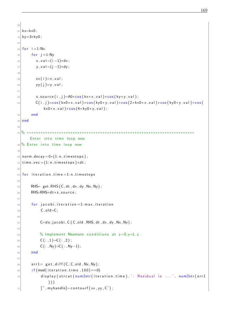
169
30
31 kx=kx0 ;
32 ky=3∗ky0 ;
33
34 f o r i =1:Nx
35 f o r j =1:Ny
36 x v a l =( i −1)∗dx ;
37 y v a l =( j −1)∗dy ;
38
39 xx ( i )=x v a l ;
40 yy ( j )=y v a l ;
41
42 s s o u r c e ( i , j )=A0∗ cos ( kx∗ x v a l ) ∗ cos ( ky∗ y v a l ) ;
43 C( i , j )=cos ( kx0∗ x v a l ) ∗ cos ( ky0∗ y v a l )+cos (2∗ kx0∗ x v a l ) ∗ cos ( ky0∗ y v a l )+cos (
kx0∗ x v a l ) ∗ cos (4∗ ky0∗ y v a l ) ;
44 end
45 end
46
47 % ∗∗∗∗∗∗∗∗∗∗∗∗∗∗∗∗∗∗∗∗∗∗∗∗∗∗∗∗∗∗∗∗∗∗∗∗∗∗∗∗∗∗∗∗∗∗∗∗∗∗∗∗∗∗∗∗∗∗∗∗∗∗∗∗∗∗∗∗∗∗∗∗∗E n t e r i n t o t ime l o o p now
48 % E n t e r i n t o t ime l o o p now
49
50 norm decay =0∗(1: n t i m e s t e p s ) ;
51 t i m e v e c =(1: n t i m e s t e p s ) ∗ dt ;
52
53 f o r i t e r a t i o n t i m e =1: n t i m e s t e p s
54
55 RHS= get RHS (C , dt , dx , dy , Nx , Ny) ;
56 RHS=RHS+dt ∗ s s o u r c e ;
57
58 f o r j a c o b i i t e r a t i o n =1: m a x i t e r a t i o n
59 C o l d=C ;
60
61 C=d o j a c o b i C ( C old , RHS, dt , dx , dy , Nx , Ny) ;
62
63 % Implement Neumann c o n d i t i o n s at y=0,y=L y .
64 C ( : , 1 )=C ( : , 2 ) ;
65 C ( : , Ny)=C ( : , Ny−1) ;
66 end
67
68 e r r 1= g e t d i f f (C , C old , Nx , Ny) ;
69 i f (mod( i t e r a t i o n t i m e , 1 0 0 ) ==0)
70 d i s p l a y ( s t r c a t ( num2str ( i t e r a t i o n t i m e ) , ’ : R e s i d u a l i s . . . ’ , num2str ( e r r 1
) ) )
71 [ ˜ , myhandle ]= c o n t o u r f ( xx , yy , C ’ ) ;
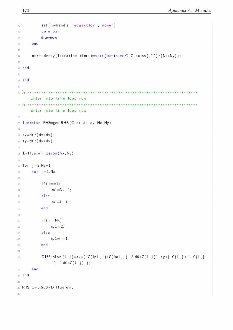
170 Appendix A. M codes
72 s e t ( myhandle , ’ e d g e c o l o r ’ , ’ none ’ ) ;
73 c o l o r b a r
74 drawnow
75 end
76
77 norm decay ( i t e r a t i o n t i m e )=s q r t ( sum ( sum (C−C p o i s s ) . ˆ 2 ) /(Nx∗Ny) ) ;
78
79 end
80
81 end
82
83 % ∗∗∗∗∗∗∗∗∗∗∗∗∗∗∗∗∗∗∗∗∗∗∗∗∗∗∗∗∗∗∗∗∗∗∗∗∗∗∗∗∗∗∗∗∗∗∗∗∗∗∗∗∗∗∗∗∗∗∗∗∗∗∗∗∗∗∗∗∗∗∗∗∗E n t e r i n t o t ime l o o p now
84 % ∗∗∗∗∗∗∗∗∗∗∗∗∗∗∗∗∗∗∗∗∗∗∗∗∗∗∗∗∗∗∗∗∗∗∗∗∗∗∗∗∗∗∗∗∗∗∗∗∗∗∗∗∗∗∗∗∗∗∗∗∗∗∗∗∗∗∗∗∗∗∗∗∗E n t e r i n t o t ime l o o p now
85
86 f u n c t i o n RHS=get RHS (C , dt , dx , dy , Nx , Ny)
87
88 ax=dt /( dx∗dx ) ;
89 ay=dt /( dy∗dy ) ;
90
91 D i f f u s i o n=z e r o s (Nx , Ny) ;
92
93 f o r j =2:Ny−1
94 f o r i =1:Nx
95
96 i f ( i ==1)
97 im1=Nx−1;
98 e l s e
99 im1=i −1;
100 end
101
102 i f ( i==Nx)
103 i p 1 =2;
104 e l s e
105 i p 1=i +1;
106 end
107
108 D i f f u s i o n ( i , j )=ax ∗( C( ip1 , j )+C( im1 , j )−2.d0∗C( i , j ) )+ay ∗( C( i , j +1)+C( i , j
−1)−2.d0∗C( i , j ) ) ;
109 end
110 end
111
112 RHS=C+0.5 d0∗ D i f f u s i o n ;
113

171
114 end
115
116 % ∗∗∗∗∗∗∗∗∗∗∗∗∗∗∗∗∗∗∗∗∗∗∗∗∗∗∗∗∗∗∗∗∗∗∗∗∗∗∗∗∗∗∗∗∗∗∗∗∗∗∗∗∗∗∗∗∗∗∗∗∗∗∗∗∗∗∗∗∗∗∗∗∗E n t e r i n t o t ime l o o p now
117
118 f u n c t i o n C=d o j a c o b i C ( C old , RHS, dt , dx , dy , Nx , Ny)
119
120 ax=dt /( dx∗dx ) ;
121 ay=dt /( dy∗dy ) ;
122 d i a g v a l=1+ax+ay ;
123
124 C=z e r o s (Nx , Ny) ;
125
126 f o r j =2:Ny−1
127 f o r i =1:Nx
128
129 i f ( i ==1)
130 im1=Nx−1;
131 e l s e
132 im1=i −1;
133 end
134
135 i f ( i==Nx)
136 i p 1 =2;
137 e l s e
138 i p 1=i +1;
139 end
140
141 t e m p v a l =(ax / 2 . d0 ) ∗( C o l d ( ip1 , j )+C o l d ( im1 , j ) )+(ay / 2 . d0 ) ∗( C o l d ( i , j +1)+C o l d
( i , j −1) )+RHS( i , j ) ;
142 C( i , j )=t e m p v a l / d i a g v a l ;
143 end
144 end
145
146 end
147
148 % ∗∗∗∗∗∗∗∗∗∗∗∗∗∗∗∗∗∗∗∗∗∗∗∗∗∗∗∗∗∗∗∗∗∗∗∗∗∗∗∗∗∗∗∗∗∗∗∗∗∗∗∗∗∗∗∗∗∗∗∗∗∗∗∗∗∗∗∗∗∗∗∗∗E n t e r i n t o t ime l o o p now
149
150 f u n c t i o n e r r 1=g e t d i f f (C , C old , ˜ , ˜ )
151
152 e r r 1=max ( max ( abs (C−C o l d ) ) ) ;
153
154 end
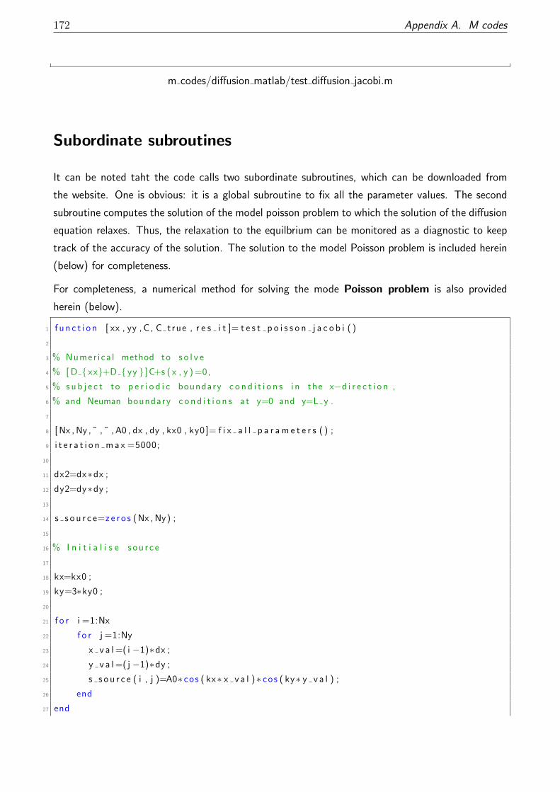
172 Appendix A. M codes
m codes/diffusion matlab/test diffusion jacobi.m
Subordinate subroutines
It can be noted taht the code calls two subordinate subroutines, which can be downloaded from
the website. One is obvious: it is a global subroutine to fix all the parameter values. The second
subroutine computes the solution of the model poisson problem to which the solution of the diffusion
equation relaxes. Thus, the relaxation to the equilbrium can be monitored as a diagnostic to keep
track of the accuracy of the solution. The solution to the model Poisson problem is included herein
(below) for completeness.
For completeness, a numerical method for solving the mode Poisson problem is also provided
herein (below).
1 f u n c t i o n [ xx , yy , C , C t rue , r e s i t ]= t e s t p o i s s o n j a c o b i ( )
2
3 % Numer i ca l method to s o l v e
4 % [ D xx+D yy ]C+s ( x , y ) =0,
5 % s u b j e c t to p e r i o d i c boundary c o n d i t i o n s i n the x−d i r e c t i o n ,
6 % and Neuman boundary c o n d i t i o n s at y=0 and y=L y .
7
8 [ Nx , Ny , ˜ , ˜ , A0 , dx , dy , kx0 , ky0 ]= f i x a l l p a r a m e t e r s ( ) ;
9 i t e r a t i o n m a x =5000;
10
11 dx2=dx∗dx ;
12 dy2=dy∗dy ;
13
14 s s o u r c e=z e r o s (Nx , Ny) ;
15
16 % I n i t i a l i s e s o u r c e
17
18 kx=kx0 ;
19 ky=3∗ky0 ;
20
21 f o r i =1:Nx
22 f o r j =1:Ny
23 x v a l =( i −1)∗dx ;
24 y v a l =( j −1)∗dy ;
25 s s o u r c e ( i , j )=A0∗ cos ( kx∗ x v a l ) ∗ cos ( ky∗ y v a l ) ;
26 end
27 end

173
28
29 % Compute a n a l y t i c s o l u t i o n ∗∗∗∗∗∗∗∗∗∗∗∗∗∗∗∗∗∗∗∗∗∗∗∗∗∗∗∗∗∗∗∗∗∗∗∗∗∗∗∗∗∗∗∗∗∗∗30
31
32 xx =0∗(1:Nx) ;
33 yy =0∗(1:Ny) ;
34 C t r u e=z e r o s (Nx , Ny) ;
35
36 f o r i =1:Nx
37 f o r j =1:Ny
38 xx ( i )=( i −1)∗dx ;
39 yy ( j )=( j −1)∗dy ;
40
41 C t r u e ( i , j )=(A0/( kx∗kx+ky∗ky ) ) ∗ cos ( kx∗ xx ( i ) ) ∗ cos ( ky∗ yy ( j ) ) ;
42
43 end
44 end
45
46 % I t e r a t i o n s t e p ∗∗∗∗∗∗∗∗∗∗∗∗∗∗∗∗∗∗∗∗∗∗∗∗∗∗∗∗∗∗∗∗∗∗∗∗∗∗∗∗∗∗∗∗∗∗∗∗∗∗∗∗∗∗∗∗∗∗47 % I n i t i a l g u e s s f o r C :
48 C=z e r o s (Nx , Ny) ;
49
50 r e s i t =0∗(1: i t e r a t i o n m a x ) ;
51
52 f o r i t e r a t i o n =1: i t e r a t i o n m a x
53
54 C o l d=C ;
55
56 f o r i =1:Nx
57
58 % P e r i o d i c BCs h e r e .
59 i f ( i ==1)
60 im1=Nx−1;
61 e l s e
62 im1=i −1;
63 end
64
65 i f ( i==Nx)
66 i p 1 =2;
67 e l s e
68 i p 1=i +1;
69 end
70
71 f o r j =2:Ny−1
72

174 Appendix A. M codes
73 d i a g o n a l =(2. d0/ dx2 ) +(2. d0/ dy2 ) ;
74 tempva l =(1. d0/ dx2 ) ∗( C o l d ( ip1 , j )+C o l d ( im1 , j ) ) +(1. d0/ dy2 ) ∗( C o l d ( i , j
+1)+C o l d ( i , j −1) )+s s o u r c e ( i , j ) ;
75 C( i , j )=tempva l / d i a g o n a l ;
76
77 end
78 end
79
80 % Implement D i r i c h l e t c o n d i t i o n s a t y=0,y=L y .
81 C ( : , 1 )=C ( : , 2 ) ;
82 C ( : , Ny)=C ( : , Ny−1) ;
83
84 r e s i t ( i t e r a t i o n )=max ( max ( abs (C−C o l d ) ) ) ;
85
86 end
87
88 end
m codes/diffusion matlab/test poisson jacobi.m

Appendix B
Introduction to Fortran
Overview
I am going to try an example-based introduction to Fortran, wherein I provide you with a sample
code, and then tell you about it. I will then ask you to some tasks based on the code, and to modify
it.
B.1 Preliminaries
A basic Fortran code is written in a single file with a .f90 file extension. It conists of a main part
together with subroutine definitions. A subroutine is like a subfunction in Matlab or C, with one
key difference that I will explain below.
The main part
The main code is enclosed by the following declaration pair:
program mainprogram
...
end program mainprogram
At the top level, all variables that are to be used must be declared (otherwise compiler errors
will ensue). Variables can be declared as integers or as double-precision numbers (other types are
possible and will be discussed later on). Before variable declarations are made, a good idea is to
type implicit none. This means that Fortran will not assume that symbols such as i have an
175
176 Appendix B. Introduction to Fortran
(implicit) type. It is best to be honest with the compiler and tell it upfront what you are going to
do. Equally, it is not a good idea for the compiler to try to guess what you mean.
An array of double-precision numbers is defined as follows:
integer :: Nx,Ny
parameter (Nx = 201, Ny = 101)
double precision, dimension(1:Nx,1:Ny) :: my_array
This creates an array of double-precision numbers where the indices go from i = 1, 2, · · · , 201, and
j = 1, 2, · · · , 101. there is nothing special in Fortran about starting arrays with i = 1: they can
start from any integer whatsoever (positive or negative).
After defining all arrays and all other variables operations are performed on them using standard
manipulations. These typically include ‘do’ loops (the Fortran equivalent of ‘for’ loops), and ‘if’ and
‘if-else’ statements. The syntax for these operatiosn is given below in the sample code (Section B.2).
Column-major ordering
To understand column-major ordering, consider the following array:
A =
[1 2 3
4 5 6
]
If stored in contiguous memory in a column-major format, this array will take the following form in
memory:
1 4 2 5 3 6.
Suppose that elements of the array A are denoted by Aij (i for rows, j for columns). When these
elements are accessed sequentially in contiguous memory, it is the row index that increases the
fastest. Thus, in Fortran, a do loop for manipulations on the array A should be written out as
follows:
do j=1,2
do i=1,3
! manipulations on A(i,j) here
...
end do
end do

B.1. Preliminaries 177
Subroutines
Subroutines contain discrete tasks that are repeated many times. Instead of having a main code that
contains multiple copies of the same piece of code, such code-tasks are relegated to subroutines.
The advantages are economy-of-code and computational efficiency. Unlike in C, arrays can be passed
to subroutines in a blindly straightforward manner. Examples of such subroutines can be found in
the sample code (Section B.2).
As mentioned previously, a subroutine in Fortran is like a subfunction in C or Matlab. However,
there is one key difference: formally, a subroutine produces no explicit outputs. Thus, suppose
we want to operate on a variable x with an operation f to give a result y (formally, y = f(x)). In
Fortran, we view x and y as inputs to a subroutine wherein y is assigned the value f(x) as part of
the subroutine’s implementation. This will become clearer in examples.
Output
Finally, the result of these manipulations should be sent to a file, for subsequent reading. The values
in an array my array of size (1, · · · , Nx)× (1, · · ·Ny) can be written to a file as follows:
open(unit=20,file=’myfile.dat’,status=’UNKNOWN’)
do j=1,Ny
do i=1,Nx
write(20,*) my_array(i,j)
end do
end do
close(unit=20, status=’KEEP’)

178 Appendix B. Introduction to Fortran
B.2 The code
The following code solves the model Poisson problem using SOR iteration. If done correctly, it
should reproduce exactly the results obtained previously in Matlab. An output file called ‘oned.dat’
is produced. I cannot remember why I called the output file by this name. However, these things
are rather arbitrary.
1 ! ∗∗∗∗∗∗∗∗∗∗∗∗∗∗∗∗∗∗∗∗∗∗∗∗∗∗∗∗∗∗∗∗∗∗∗∗∗∗∗∗∗∗∗∗∗∗∗∗∗∗∗∗∗∗∗∗∗∗∗∗∗∗2
3 program mainprogram
4 i m p l i c i t none
5
6 i n t e g e r : : Nx , Ny
7 pa ra me te r (Nx = 201 , Ny = 101)
8
9 d o u b l e p r e c i s i o n : : dx , dy , x v a l , y v a l , Lx , Ly , p i =3.1415926535
10 d o u b l e p r e c i s i o n : : ax , ay , d i a g v a l , r e l a x , tempval , e r r 1 , e r r 2 , A0
11 d o u b l e p r e c i s i o n , d i m e n s i o n ( 1 : Nx , 1 : Ny) : : f s o u r c e , C , C o l d
12
13 i n t e g e r : : i , j , im1 , ip1 , i t e r a t i o n , m a x i t e r a t i o n =1000
14
15 Lx =2. d0
16 Ly =1. d0
17
18 A0=10. d0
19
20 dx=Lx/ d b l e (Nx−1)
21 dy=Ly/ d b l e (Ny−1)
22
23 ax =1. d0 /( dx∗dx )
24 ay =1. d0 /( dy∗dy )
25 d i a g v a l =2. d0∗ax +2. d0∗ay
26 r e l a x =1.5 d0
27
28 ! ∗∗∗∗∗∗∗∗∗∗∗∗∗∗∗∗∗∗∗∗∗∗∗∗∗∗∗∗∗∗∗∗∗∗∗∗∗∗∗∗∗∗∗∗∗∗∗∗∗∗∗∗∗∗∗∗∗∗∗∗∗∗29 ! compute s o u r c e , i n i t i a l i s e g u e s s
30
31 f s o u r c e =0. d0
32 C=0. d0
33 C o l d =0. d0
34
35 w r i t e (∗ ,∗ ) ’ g e t t i n g s o u r c e ’
36 c a l l g e t f p e r i o d i c ( f s o u r c e , Nx , Ny , dx , dy , Lx , Ly , A0)
37 w r i t e (∗ ,∗ ) ’ done ’
38

B.2. The code 179
39 ! ∗∗∗∗∗∗∗∗∗∗∗∗∗∗∗∗∗∗∗∗∗∗∗∗∗∗∗∗∗∗∗∗∗∗∗∗∗∗∗∗∗∗∗∗∗∗∗∗∗∗∗∗∗∗∗∗∗∗∗∗∗∗40 ! s o r s t e p s
41
42 do i t e r a t i o n =1, m a x i t e r a t i o n
43 e r r 1 = 0 . 0
44
45 ! f o r k e e p i n g t r a c k o f t he e r r o r
46 C o l d=C
47
48 do j = 2 ,Ny−1
49 do i = 1 ,Nx
50
51 i f ( i . eq . 1 ) then
52 im1=Nx−1
53 e l s e
54 im1=i−1
55 end i f
56
57 i f ( i . eq . Nx) then
58 i p 1=2
59 e l s e
60 i p 1=i +1
61 end i f
62
63 tempva l=ax ∗(C( ip1 , j )+C( im1 , j ) )+ay ∗(C( i , j +1)+C( i , j −1) )− f s o u r c e ( i , j
)
64 C( i , j )=(1− r e l a x ) ∗C( i , j )+r e l a x ∗ tempva l / d i a g v a l
65
66 end do
67 end do
68
69 ! Implement D i r i c h l e t c o n d i t i o n s a t y=0,y=L y .
70 C ( : , 1 )=C ( : , 2 )
71 C ( : , Ny)=C ( : , Ny−1)
72
73 i f (mod( i t e r a t i o n , 1 0 0 ) ==0)then
74 c a l l g e t d i f f (C , C old , Nx , Ny , e r r 1 )
75 w r i t e (∗ ,∗ ) i t e r a t i o n , ’ D i f f e r e n c e i s ’ , e r r 1
76 end I f
77
78 end do
79
80 w r i t e (∗ ,∗ ) ’ D i f f e r e n c e i s ’ , e r r 1
81
82

180 Appendix B. Introduction to Fortran
83 ! ∗∗∗∗∗∗∗∗∗∗∗∗∗∗∗∗∗∗∗∗∗∗∗∗∗∗∗∗∗∗∗∗∗∗∗∗∗∗∗∗∗∗∗∗∗∗∗∗∗∗∗∗∗∗∗∗∗∗∗∗∗∗84 ! w r i t e r e s u l t to f i l e
85
86 w r i t e (∗ ,∗ ) ’ w r i t i n g to f i l e ’
87 open ( u n i t =20, f i l e = ’ oned . dat ’ , s t a t u s= ’UNKNOWN’ )
88
89 do j =1,Ny
90 do i =1,Nx
91 x v a l =( i −1)∗dx
92 y v a l =( j −1)∗dy
93 Write ( 2 0 ,∗ ) x v a l , y v a l , C( i , j )
94 end do
95 end do
96 c l o s e ( u n i t =20, s t a t u s= ’KEEP ’ )
97 w r i t e (∗ ,∗ ) ’ done ’
98
99 end program mainprogram
100
101
102 ! ∗∗∗∗∗∗∗∗∗∗∗∗∗∗∗∗∗∗∗∗∗∗∗∗∗∗∗∗∗∗∗∗∗∗∗∗∗∗∗∗∗∗∗∗∗∗∗∗∗∗∗∗∗∗∗∗∗∗∗∗∗∗103 ! ∗∗∗∗∗∗∗∗∗∗∗∗∗∗∗∗∗∗∗∗∗∗∗∗∗∗∗∗∗∗∗∗∗∗∗∗∗∗∗∗∗∗∗∗∗∗∗∗∗∗∗∗∗∗∗∗∗∗∗∗∗∗104
105 s u b r o u t i n e g e t f p e r i o d i c ( f s r c , Nx , Ny , dx , dy , Lx , Ly , A0)
106 i m p l i c i t none
107
108 i n t e g e r : : i , j , Nx , Ny
109 d o u b l e p r e c i s i o n : : dx , dy , Lx , Ly , x v a l , y v a l , p i =3.1415926535
110 d o u b l e p r e c i s i o n : : kx0 , ky0 , kx , ky , A0
111 d o u b l e p r e c i s i o n : : f s r c ( 1 : Nx , 1 : Ny)
112
113 kx0 =2. d0∗ p i /Lx
114 ky0=p i /Ly
115
116 kx=kx0
117 ky =3. d0∗ky0
118
119 f s r c =0. d0
120 do j =1,Ny
121 do i =1,Nx
122 x v a l =( i −1)∗dx
123 y v a l =( j −1)∗dy
124 f s r c ( i , j )=A0∗ cos ( kx∗ x v a l ) ∗ cos ( ky∗ y v a l )
125 end do
126 end do
127

B.2. The code 181
128 r e t u r n
129 end s u b r o u t i n e g e t f p e r i o d i c
130
131 ! ∗∗∗∗∗∗∗∗∗∗∗∗∗∗∗∗∗∗∗∗∗∗∗∗∗∗∗∗∗∗∗∗∗∗∗∗∗∗∗∗∗∗∗∗∗∗∗∗∗∗∗∗∗∗∗∗∗∗∗∗∗∗132
133 s u b r o u t i n e g e t d i f f (C , C old , Nx , Ny , d i f f )
134 i m p l i c i t none
135
136 d o u b l e p r e c i s i o n : : d i f f , sum
137 i n t e g e r : : Nx , Ny , i , j
138 d o u b l e p r e c i s i o n , d i m e n s i o n ( 1 : Nx , 1 : Ny) : : C , C o l d
139
140 sum = 0 . 0 D0
141 Do j = 1 , Ny
142 Do i = 1 , Nx
143 sum = sum + (C( i , j )−C o l d ( i , j ) ) ∗∗2
144 End Do
145 End Do
146 d i f f = sum
147
148 Return
149 End s u b r o u t i n e g e t d i f f
150
151 ! ∗∗∗∗∗∗∗∗∗∗∗∗∗∗∗∗∗∗∗∗∗∗∗∗∗∗∗∗∗∗∗∗∗∗∗∗∗∗∗∗∗∗∗∗∗∗∗∗∗∗∗∗∗∗∗∗∗∗∗∗∗∗152 ! ∗∗∗∗∗∗∗∗∗∗∗∗∗∗∗∗∗∗∗∗∗∗∗∗∗∗∗∗∗∗∗∗∗∗∗∗∗∗∗∗∗∗∗∗∗∗∗∗∗∗∗∗∗∗∗∗∗∗∗∗∗∗
m codes/poisson code/main periodic sor.f90

182 Appendix B. Introduction to Fortran
B.3 Porting Output into Matlab
It can be useful to examine the data in a file such as ‘oned.dat’ in Matlab. There are many ways of
doing this. Below is my favourite way:
1 f u n c t i o n [ X, Y, C]= o p e n d a t f i l e ( )
2
3 % We need to s p e c i f y t he s i z e o f t he c o m p u t a t i o n a l domain , as t h i s can ’ t be
4 % i n f e r r e d from t he d a t a f i l e .
5
6 Nx=201;
7 Ny=101;
8
9 % Here I c r e a t e a c h a r a c t e r a r r a y c a l l e d ” f i l e n a m e ” . Th i s s h o u l d
10 % c o r r e s p o n d to t he name o f t he F o r t r a n−g e n e r a t e d f i l e .
11
12 f i l e n a m e= ’ oned . dat ’ ;
13
14 % Here i s th e number o f l i n e s i n th e d a t a f i l e .
15 n l i n e s=Nx∗Ny ;
16
17 % Open th e f i l e . Here , f i d i s a l a b e l t h a t l a b e l s which l i n e i n th e f i l e
18 % i s b e i n g r e a d . O b v i o u s l y , upon o p e n i n g th e f i l e , we a r e at l i n e 1 .
19
20 f i d=fo pe n ( f i l e n a m e ) ;
21
22 % P r e a l l o c a t e some a r r a y s f o r s t o r i n g t he data .
23
24 X=0∗(1: n l i n e s ) ;
25 Y=0∗(1: n l i n e s ) ;
26 C=0∗(1: n l i n e s ) ;
27
28 % Loop o v e r a l l l i n e s .
29
30 f o r i =1: n l i n e s
31 % Grab t he data from t he c u r r e n t l i n e . Once t he data i s grabbed , the
32 % l a b e l f i x a u t o m a t i c a l l y moves on to th e n e x t l i n e .
33 % The data from the c u r r e n t l i n e i s grabbed i n t o a s t r i n g − h e r e c a l l e d
34 % c1 .
35 c1=f g e t l ( f i d ) ;
36
37 % Next I have to c o n v e r t th e t h r e e s t r i n g s on any g i v e n l i n e i n t o t h r e e
38 % d o u b l e s . Th i s i s done by s c a n n i n g th e s t r i n g i n t o an a r r a y o f
39 % d o u b l e s , u s i n g th e ” s s c a n f ” command :
40 vec temp=s s c a n f ( c1 , ’%f ’ ) ;
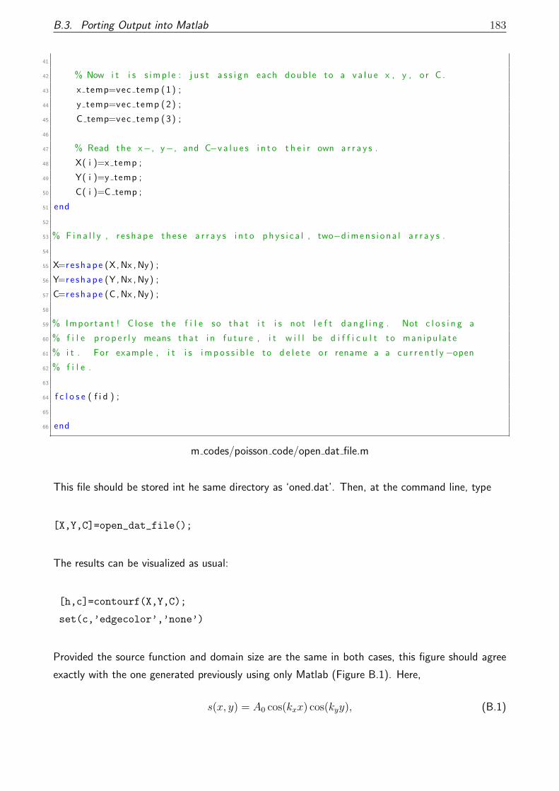
B.3. Porting Output into Matlab 183
41
42 % Now i t i s s i m p l e : j u s t a s s i g n each d o u b l e to a v a l u e x , y , o r C .
43 x temp=vec temp ( 1 ) ;
44 y temp=vec temp ( 2 ) ;
45 C temp=vec temp ( 3 ) ;
46
47 % Read t he x−, y−, and C−v a l u e s i n t o t h e i r own a r r a y s .
48 X( i )=x temp ;
49 Y( i )=y temp ;
50 C( i )=C temp ;
51 end
52
53 % F i n a l l y , r e s h a p e t h e s e a r r a y s i n t o p h y s i c a l , two−d i m e n s i o n a l a r r a y s .
54
55 X=r e s h a p e (X, Nx , Ny) ;
56 Y=r e s h a p e (Y, Nx , Ny) ;
57 C=r e s h a p e (C , Nx , Ny) ;
58
59 % I m p o r t a n t ! C l o s e th e f i l e so t h a t i t i s not l e f t d a n g l i n g . Not c l o s i n g a
60 % f i l e p r o p e r l y means t h a t i n f u t u r e , i t w i l l be d i f f i c u l t to m a n i p u l a t e
61 % i t . For example , i t i s i m p o s s i b l e to d e l e t e o r rename a a c u r r e n t l y−open
62 % f i l e .
63
64 f c l o s e ( f i d ) ;
65
66 end
m codes/poisson code/open dat file.m
This file should be stored int he same directory as ‘oned.dat’. Then, at the command line, type
[X,Y,C]=open_dat_file();
The results can be visualized as usual:
[h,c]=contourf(X,Y,C);
set(c,’edgecolor’,’none’)
Provided the source function and domain size are the same in both cases, this figure should agree
exactly with the one generated previously using only Matlab (Figure B.1). Here,
s(x, y) = A0 cos(kxx) cos(kyy), (B.1)

184 Appendix B. Introduction to Fortran
with kx = kx0 and ky = 3ky0, and A0 = 10. Further details: kx0 = (2π/Lx) is the fundamental
wavenumber in the x-direction, and ky0 = π/Ly is the fundamental wewavenumber in the y-
direction. The domain geometry is chosen to be Lx = 2 and Ly = 1.
Figure B.1: Solution of the Poisson problem for the source (B.1). Grid size: Nx = 201 andNy = 101.

Bibliography
[AB97] M. B. Abbott and R. Basco. Computational Fluid Dynamics – An Introduction for
Engineers. Longman, 1997.
[Are84] Hassan Aref. Stirring by chaotic advection. Journal of fluid mechanics, 143:1–21, 1984.
[BBP08] C. Benocci, J. V. Beeck, and U. Piomelli. Large eddy simulation and related techniques
theory and applications, 2008. VKI Lecturer Series.
[BC78] E. K. Blum and A. F. Chang. A numerical method for the solution of the double
eigenvalue problem. IMA J. Appl. Math., 22:29–42, 1978.
[BCF95] Pierre Barthelet, Francois Charru, and Jean Fabre. Experimental study of interfacial long
waves in a two-layer shear flow. Journal of Fluid Mechanics, 303:23–53, 1995.
[BGC04] Paul Batten, Uriel Goldberg, and Sukumar Chakravarthy. Interfacing statistical turbu-
lence closures with large-eddy simulation. AIAA journal, 42(3):485–492, 2004.
[Bib07] D. Biberg. A mathematical model for two-phase stratified turbulent duct flow. Multiph.
Sci.Tech., 19:1, 2007.
[Boy01] J. P. Boyd. Chebyshev and Fourier Spectral Methods. Dover, 2001.
[CC97] C. Cossu and J. M. Chomaz. Global measures of local convective instabilities. Phys.
Rev. Lett., 78:4387–4390, 1997.
[Cha61] S. Chandrasekhar. Hydrodynamic and Hydromagnetic Stability. Dover, New York, 1961.
[Dav09] P. A. Davidson. Turbulence – An Introduction for Scientists and Engineers. Oxford
University Press, 2009.
[Dea70] James W Deardorff. A numerical study of three-dimensional turbulent channel flow at
large reynolds numbers. Journal of Fluid Mechanics, 41(02):453–480, 1970.
[DR81] P. G. Drazin and W. H. Reid. Hydrodynamic Stability. Cambridge University Press,
Cambridge, UK, 1981.
185

186 BIBLIOGRAPHY
[Gov] V. Govorukhin. Computer code, ode87 integrator. Downloaded at
http://www.mathworks.com/matlabcentral/fileexchange/3616-ode87-integrator.
[Gra09] E.-M. Graefe. Quantum-Classical Correspondence for a Bose-Hubbard dimer and its
non-Hermitian generalisation. PhD thesis, Technische Universitat Kaiserslautern, 2009.
[Gro00] S. Grossmann. The onset of shear flow turbulence. Rev. Mod. Phys., 72:603–618, 2000.
[HM90] P. Huerre and P. A. Monkewitz. Local and global instability in spatially developing flows.
Ann. Rev. Fluid Mech., 22:473–537, 1990.
[Mas94] Paul J Mason. Large-eddy simulation: A critical review of the technique. Quarterly
Journal of the Royal Meteorological Society, 120(515):1–26, 1994.
[Mon88] P. A. Monkewitz. The absolute and convective nature of instability in two-dimensional
wakes at low Reynolds numbers. Phys. Fluids, 31:999, 1988.
[NS13] Lennon O Naraigh and Peter DM Spelt. An analytical connection between temporal and
spatio-temporal growth rates in linear stability analysis. Proceedings of the Royal Society
A: Mathematical, Physical and Engineering Science, 469(2156):20130171, 2013.
[NSMZ11] L O Naraigh, Peter DM Spelt, OK Matar, and TA Zaki. Interfacial instability in turbulent
flow over a liquid film in a channel. International Journal of Multiphase Flow, 37(7):812–
830, 2011.
[NSN15] Lennon O Naraigh, Selma Shun, and Aurore Naso. Flow-parametric regulation of shear-
driven phase separation in two and three dimensions. Physical Review E, 91:062127,
2015.
[ONSS13] Lennon O Naraigh, Peter DM Spelt, and Stephen J Shaw. Absolute linear instability
in laminar and turbulent gas–liquid two-layer channel flow. Journal of Fluid Mechanics,
714:58–94, 2013.
[Orz71] S. A. Orzag. Accurate solution of the Orr–Sommerfeld equation. J. Fluid Mech., 50:689,
1971.
[Pio93] Ugo Piomelli. High reynolds number calculations using the dynamic subgrid-scale stress
model. Physics of Fluids A: Fluid Dynamics (1989-1993), 5(6):1484–1490, 1993.
[Pop00] S. B. Pope. Turbulent Flows. Cambridge University Press, Cambridge, UK, 2000.
[Rom73] VA Romanov. Stability of plane-parallel couette flow. Functional analysis and its appli-
cations, 7(2):137–146, 1973.

BIBLIOGRAPHY 187
[Rot09] I. Rotter. A non-hermitian hamilton operator and the physics of open quantum systems.
J. Phys. A: Math. Theor., 42:153001, 2009.
[San09] K. Sangodoyin. Computational fluid dynamics of turbulent stratified flow. Master’s
thesis, Imperial College London, 2009.
[Sch75] Ulrich Schumann. Subgrid scale model for finite difference simulations of turbulent flows
in plane channels and annuli. Journal of computational physics, 18(4):376–404, 1975.
[SH01] P. J. Schmid and D. S. Henningson. Stability and Transition in Shear Flows. Springer,
New York, 2001.
[Sma63] Joseph Smagorinsky. General circulation experiments with the primitive equations: I.
the basic experiment*. Monthly weather review, 91(3):99–164, 1963.
[tS13] L. O Naraigh and P. D. M. Spelt. An analytical connection between temporal and spatio-
temporal growth rates in linear stability analysis. Proceedings of the Royal Society A,
469(2156), 2013.
[TTTD93] N. L. Trefethen, A. E. Trefethen, S. C. Teddy, and T. A. Driscoll. Hydrodynamic stability
without eigenvalues. Science, 561:578, 1993.
[Wal95] F. Waleffe. Transition in shear flows. nonlinear normality verus nonnormal linearity. Phys.
Fluids, 7:3060–3066, 1995.
[Wal98] F. Waleffe. Three-dimensional coherent states in plane shear flows. Phys. Rev. Lett.,
81:4140–4143, 1998.
[WWL87] W. W. Willmarth, T. Wei, and C. O. Lee. Laser anemometer measurements of reynolds
stress in a turbulent channel flow with drag reducing polymer additives. Phys. Fluids,
30:933, 1987.