Uniqueness of Optimal Mod 3 Circuits for Parity Frederic Green Amitabha Roy Frederic Green Amitabha...

Uniqueness of Uniqueness of Optimal Mod 3 Optimal Mod 3

Circuits for ParityCircuits for Parity

Frederic Green Amitabha Roy Frederic Green Amitabha Roy Clark University Clark University AkamaiAkamai

€

x1

€

xn

€

K K K K K K K

€

≥

€

modm

€

K K

€

modm

€

modm

€

∧

€

∧

€

∧

€

∧

€

∧

€

∧

€

L

€

L

€

L

€

L

€

L

€

L

€

"Maj omodm o∧d " circuit

d

Goal: Lower bounds on parity for circuits of this shape:

€

≥

€

modm

€

K K

€

∧

€

∧

€

∧

€

∧

€

∧

€

∧€

modm

€

modm

€

L

€

L

€

L

€

L

€

L

€

L

€

x1

€

xn

€

K K K K K K K

€

≥

€

modm

€

K K

€

∧

€

∧

€

∧

€

∧

€

∧

€

∧

€

x1

€

xn

€

K K K K K K K

Reduces to: Upper bounds bounds on correlation:

€

modm

€

modm

€

L

€

L

€

L

€

L

€

L

€

L

s

Hajnal et al.: Correlation with parity < here

s > 1/

implies

d

Correlation:Defn: normalized # of agreements-disagreements:

€

C( f ,g) =1

2n(−1) f (x )+g(x )

x ∈{0,1}n

∑

In this case: interested in f = the parity function:

and g computed by a polynomial mod m of degree d, for odd m:

€

f (x) = x i

i=1

n

∑ mod 2x1 x2 xn

. . .

€

1 if p(x1,...,xn ) ≡ 0 mod m

0 otherwise

€

g(x) =

€

∧

€

∧

€

modm

€

L

€

L

. . .

€

• Maj omodm o∧polylog(n) are powerful; they cansimulate any AC0 circuit in quasipolynomial size.[Allender, 1990]

• …and yet we don't know if they can simulate any more of ACC (e.g., parity).

Many reasons. Here are two:

€

• By Hastad/Boppana [1986], C(⊕, f ) is O(2-nε

) if f is an AC 0 function. By Razborov/Smolensky [1987], if f is ACC(p) the correlation is O(1/n1/ 2−o(1)). Is it really that big in that case?

Main concern here: m = 3, d = 2:

€

≥

€

mod3

€

mod3

€

mod3

€

K K

€

∧

€

∧

€

∧

€

∧

€

∧

€

∧

€

x1

€

xn

€

K K K K K K K

d < 2

€

S(t,k,n) =1

2nχ x i

i=1

n

∏ ⎛

⎝ ⎜

⎞

⎠ ⎟

x∈Z3n

∑ ω t(x1 .K ,xn )+k(x1 .K ,xn )+ c

Reduction to Exponential Sums

€

C(⊕, mod3o∧2) =4

3ℜ S(t,k,n)( )

where,

The correlation can be related to an exponential sum,[Cai, Green & Thierauf 1996], like those that arise innumber theory.

When m = 3, this reduction is especially simple (e.g., d=2):

€

(here χ : Z3 → C is the multiplicative character (χ (0) = 0, χ (±1) = ±1),ω = e2π i / 3 is the primitive 3rd root of unity, t is a quadratic form, k is alinear form, and c is a constant. Note χ (0) = 0 ⇒ x ∈ {1,−1}n .)

Generalizations

€

Of course, S(t,k,n) can be generalized to other moduli mand higher degree p : Sm (p,n).

€

Can also consider Modq versus polynomials in Zm ,(q,m) =1.

€

In both cases, the idea is that upper bounds ona quantity like Sm ( p,n) give upper bounds onthe correlation.

Recent History (since ca. 2001)

€

•∀n, S3(t,k,n) ≤ 3 /2( )n / 2⎡ ⎤

[Green, JCSS 2004]

Here are some things we now know:

€

•∀ odd m, deg(p) < c lg(n) ⇒ ∀n, Sm ( p,n) ≤ 2−nε

[Bourgain, CR 2005]

€

• Similar for Modq vs. Modm for (q,m) =1 [Green, Roy & Straubing, CR 2005]

€

• Improvements (higher c) of above by Viola/Wigderson [CCC 2007] and Chattopadyay [FOCS 2007]

€

• Exp. small results for large classes of polynomials, many of high degree [Gál & Trifonov, MFCS 2006]

€

•∀ odd m, 1≤ n ≤10, Sm (t,k,n) ≤ cos(π /(2m))( )n / 2⎡ ⎤

[Dueñez, Miller, Roy & Straubing, JNT 2006]

Results Known to be Tight

€

•∀n, S3(t,k,n) ≤ 3 /2( )n / 2⎡ ⎤

[Green, JCSS 2004]

Exhaustive list:

€



Can We Get Tighter Results?

€

•∀n, S3(t,k,n) ≤ 3 /2( )n / 2⎡ ⎤

[Green, JCSS 2004]

€

• Not satisfying that the above is only known as far as n =10!

€

• Many open questions left even in the quadratic case.

€

• Bourgain's technique does not work for degree higher than lg n.

€

• Our ultimate interest is in Majomodm o∧polylog(n )

circuits; we must ∴ search for techniques that give tighter bounds. …wherever we can…

€



€



So: Let's see if we can extend this:

€



Two key ingredients in Dueñez et al.'s proof:• The optimal polynomials are unique.

Question: Can we even prove this when m=3?

Conjecture (Dueñez et al.): these are true for all n.

Our answer, and main result:

…to ALL n.

• There is a "gap" in the correlation between the optimal polynomials and the "first suboptimal" ones.

€

t,k suboptimal ⇒ Sm (t,k,n) ≤ cos(π /(2m)) ⋅ Sm (topt ,kopt ,n)( )

Optimal Polynomials

€

...include polynomials of the form: x1x2 + x3x4 +L + xn−1xn (n even) x1 + x2x3 +L + xn−1xn (n odd)and similar ones formed from permutations

Uniqueness Theorem: These are the only ones!

€

∀n, S(t,k,n) = ( 3 /2) n / 2⎡ ⎤ iff t(x) + k(x) is of the above form.

Gap Theorem: Anything less is "a lot" less!

€

If topt + kopt is of the above form, and t + k is not, then

S(t,k,n) ≤ 3 /2( ) ⋅ S(topt,kopt,n) .

Uniqueness Theorem: These are the only ones!

€

∀n, S(t,k,n) = ( 3 /2) n / 2⎡ ⎤ iff t(x) + k(x) is of the above form.

Uniqueness Theorem:

€

∀n, S(t,k,n) = ( 3 /2) n / 2⎡ ⎤ iff t(x) + k(x) is of the form : x1x2 +L + xn−1xn, n even x1 + x2x3 +L + xn−1xn, n odd

Proof sketch:

€

(i) ωa + ω−a = ωa 2

+ ω−a 2

(ii) ωa −ω−a = (ω −ω )χ (a)

The proof relies heavily on these identities:

Note: (i) and (ii) can be readily generalized to other moduli; but (iii) seems rather mysterious.

€

(iii) χ (1+ a)ωb + χ (1− a)ω−b = ω(a−b )2

+ ω−(a +b )2

Uniqueness Theorem Proof, continued:

• The proof is by induction on n.

• Consider the (harder) case of n odd.

• Thus our induction hypothesis is:

€

S(t,k,n −1) = ( 3 /2)(n−1)/ 2 iff t(x) + k(x) is of the form : x1x2 +L + xn−2xn−1

• It is useful to think of the graph underlying t. E.g., for the optimal polynomials:

. . . .3 4 5 61 2

x1x2x3x4 x5x6+ + + . . . .

Uniqueness Theorem Proof, continued:Wlog, write,

€

t(x1,K , xn ) = t2(x2,K , xn ) + x1r(x2,..., xn )and,

€

k(x1,K , xn ) = x1 + l(x2,K , xn )

where t2 is a quadratic form, l and r linear forms in theindicated variables.

€

Okay, how about χ (1+ a)ωb + χ (1− a)ω−b = ω(a−b )2

+ ω−(a +b )2


€

S(t,k,n) =ω −ω

2⋅1

2⋅

1

2n−1x i

i= 2

n

∏x∈{−1,1}n−1

∑ ω t2 +( l−r)2

+ ⎛

⎝ ⎜ ⎜

1

2n−1x i

i= 2

n

∏x∈{−1,1}n−1

∑ ω t2 −(l +r )2 ⎞

⎠ ⎟ ⎟

Then, summing over x1 and using (i), (ii), (iii), obtain:

Wlog, write,

€

t(x1,K , xn ) = t2(x2,K , xn ) + x1r(x2,..., xn )and,

€

k(x1,K , xn ) = x1 + l(x2,K , xn )

where t2 is a quadratic form, l and r linear forms in theindicated variables.


€

S(t,k,n) =ω −ω

2⋅

1

2⋅

1

2n−1x i

i= 2

n

∏x∈{−1,1}n−1

∑ ω t2 +( l−r)2

+ ⎛

⎝ ⎜ ⎜

1

2n−1x i

i= 2

n

∏x∈{−1,1}n−1

∑ ω t2 −(l +r )2 ⎞

⎠ ⎟ ⎟

€

Norm 3 /2

€

Each of the form S(t',k ',n −1)

€

1

€

ω

€

ω €

−ω

€

ω −ω =i 3


€

S(t,k,n) =ω −ω

2⋅

1

2⋅

1

2n−1x i

i= 2

n

∏x∈{−1,1}n−1

∑ ω t2 +( l−r)2

+ ⎛

⎝ ⎜ ⎜

1

2n−1x i

i= 2

n

∏x∈{−1,1}n−1

∑ ω t2 −(l +r )2 ⎞

⎠ ⎟ ⎟

€

Norm 3 /2

€

Each of the form S(t',k ',n −1)

€

Just enough to get the 3 /2( )n / 2⎡ ⎤

bound

…but getting back to what we set out to prove…


€

S(t,k,n) =ω −ω

2⋅

1

2⋅

1

2n−1x i

i= 2

n

∏x∈{−1,1}n−1

∑ ω t2 +( l−r)2

+ ⎛

⎝ ⎜ ⎜

1

2n−1x i

i= 2

n

∏x∈{−1,1}n−1

∑ ω t2 −(l +r )2 ⎞

⎠ ⎟ ⎟

Not hard to see:

€

S(t,k,n) is optimal ⇒ both sums on the right are optimal

Thus, by induction:

t2 + (l - r)2 and t2 - (l + r)2 are both of optimal form

Underlying graphs must hence have the same shape:

. . . .3 4 5 61 2

…but they could be differently labeled … or could they??

Uniqueness Theorem Proof, concluded:Now,

€

t2 + (l − r)2 − (t2 − (l + r)2) = −l2 − r2

Supposed to be the "difference" of two "optimal graphs":. . . .3 4 5 61 2

Such a difference consists of "loops" (or single edges):

BUT: l2+r2 has too many cross terms to represent this!

HENCE: l = r = 0, and the polynomials are identical.and t is uniquely determined from t2

Gap Theorem:

€

S(t,k,n) =ω −ω

2⋅1

2⋅

1

2n−1x i

i= 2

n

∏x∈{−1,1}n−1

∑ ω t2 +( l−r)2

+ ⎛

⎝ ⎜ ⎜

1

2n−1x i

i= 2

n

∏x∈{−1,1}n−1

∑ ω t2 −(l +r )2 ⎞

⎠ ⎟ ⎟

€

If topt + kopt is of the above form, and t + k is not, then

S(t,k,n) ≤ 3 /2( ) ⋅ S(topt,kopt,n) .

Proof sketch:

• Again by induction on n. Also, make use of uniqueness.• Start at a place we were at before:

• Easy analysis: if both of these are either optimal or suboptimal, the induction follows through.

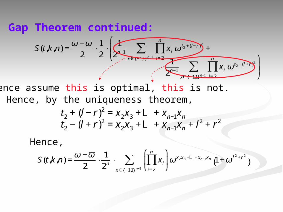
Gap Theorem continued:

€

S(t,k,n) =ω −ω

2⋅1

2⋅

1

2n−1x i

i= 2

n

∏x∈{−1,1}n−1

∑ ω t2 +( l−r)2

+ ⎛

⎝ ⎜ ⎜

1

2n−1x i

i= 2

n

∏x∈{−1,1}n−1

∑ ω t2 −(l +r )2 ⎞

⎠ ⎟ ⎟

Hence assume this is optimal, this is not.

€

t2 + (l − r)2 = x2x3 +L + xn−1xn

t2 − (l + r)2 = x2x3 +L + xn−1xn + l2 + r2

Hence, by the uniqueness theorem,

€

S(t,k,n) =ω −ω

2⋅

1

2n⋅ x i

i= 2

n

∏ ⎛

⎝ ⎜

⎞

⎠ ⎟

x∈{−1,1}n−1

∑ ω x2x3 +L +xn−1xn 1+ ω l 2 +r 2

( )

Hence,

Gap Theorem continued:

€

S(t,k,n) =ω −ω

2⋅

1

2n⋅ x i

i= 2

n

∏ ⎛

⎝ ⎜

⎞

⎠ ⎟

x∈{−1,1}n−1

∑ ω x2x3 +L +xn−1xn 1+ ω l 2 +r 2

( )

Gap Theorem concluded:

€

S(t,k,n) =ω −ω

2⋅

1

2n⋅ x i

i= 2

n

∏ ⎛

⎝ ⎜

⎞

⎠ ⎟

x∈{−1,1}n−1

∑ ω x2x3 +L +xn−1xn 1+ ω l 2 +r 2

( )

Now, this:

is not so easy to evaluate.

But if we "linearize" l2 and r2 as follows, it becomes possible:

€

ω a 2

= (ω −ω)−1(1+ ωa−1 + ω−a−1)

€

1+ ω l 2 +r 2

=2

3+

ω

3ω l + ω−l + ω r + ω−r

( )

+ω

3ω l +r + ω−l−r + ω−l +r + ω−l−r

( )

so that,


€

S(t,k,n) =ω −ω

2⋅

1

2n⋅ x i

i= 2

n

∏ ⎛

⎝ ⎜

⎞

⎠ ⎟

x∈{−1,1}n−1

∑ ω x2x3 +L +xn−1xn 1+ ω l 2 +r 2

( )

Now, this:



€

ω a 2

= (ω −ω)−1(1+ ωa−1 + ω−a−1)

€

1+ ω l 2 +r 2

=2

3

so that,


€

S(t,k,n) =ω −ω

2⋅

1

2n⋅ x i

i= 2

n

∏ ⎛

⎝ ⎜

⎞

⎠ ⎟

x∈{−1,1}n−1

∑ ω x2x3 +L +xn−1xn 1+ ω l 2 +r 2

( )

Now, this:



€

ω a 2

= (ω −ω)−1(1+ ωa−1 + ω−a−1)

€

1+ ω l 2 +r 2

=2

3+

ω

3ω l + ω−l + ω r + ω−r

( )

+ω

3ω l +r + ω−l−r + ω−l +r + ω−l−r

( )

so that,

If l, r have many terms, this dominates, giving a 1/3 factor.

Only remaining case: l, r have two terms! Gives the .

€

3 /2

Conclusions• We have proved that optimal quadratic polynomials are unique for m=3, and that there is a gap between suboptimal sums and the optimal ones. We know of no similar exact characterizations for non-trivial circuits

• Of course, we want to do this for m other than 3. How?

• Perhaps by finding other properties than uniqueness and gap that will be sufficient to push through an inductive argument?

• Perhaps by generalizing the mysterious identity (iii)?

• The problem of tight (or just tighter!) bounds for higher degrees remains a great challenge even for the m=3 case.

(well…, mostly questions):

Danke schön!

Uniqueness of Optimal Mod 3 Circuits for Parity Frederic Green Amitabha Roy Frederic Green Amitabha...

Documents

Transcript of Uniqueness of Optimal Mod 3 Circuits for Parity Frederic Green Amitabha Roy Frederic Green Amitabha...