This paper presents preliminary findings and is being distributed to economists

and other interested readers solely to stimulate discussion and elicit comments.

The views expressed in this paper are those of the authors and do not necessarily

reflect the position of the Federal Reserve Bank of New York or the Federal

Reserve System. Any errors or omissions are the responsibility of the authors.

Federal Reserve Bank of New York

Staff Reports

Understanding Mortgage Spreads

Nina Boyarchenko

Andreas Fuster

David O. Lucca

Staff Report No. 674

May 2014

Revised April 2017

Understanding Mortgage Spreads

Nina Boyarchenko, Andreas Fuster, and David O. Lucca

Federal Reserve Bank of New York Staff Reports, no. 674

May 2014; revised April 2017

JEL classification: G10, G12, G13

Abstract

Most mortgages in the United States are securitized in agency mortgage-backed securities (MBS),

and as a result, yield spreads on these securities are a key determinant of homeowners’ funding

costs. We study variation in MBS spreads over time and across securities, and document a cross-

sectional “smile” pattern in MBS spreads with respect to the securities’ coupon rates. We propose

non-interest-rate prepayment risk as a candidate driver of MBS spread variation and present a

new pricing model that uses “stripped” MBS prices to identify the contribution of this

prepayment risk to the spread. The pricing model finds that the smile can be explained by

prepayment risk, while the time-series variation is mostly accounted for by a non-prepayment risk

factor that co-moves with MBS supply and credit risk in other fixed-income markets. We use the

pricing model to study the MBS market response to the Federal Reserve’s large-scale asset

purchase program and to interpret the post-announcement divergence of spreads across MBS.

Key words: agency mortgage-backed securities, option-adjusted spreads, prepayment risk, OAS

smile

_________________

Boyarchenko, Fuster, Lucca: Federal Reserve Bank of New York (e-mails: nina.boyarchenko@ny.frb.org, andreas.fuster@ny.frb.org, david.lucca@ny.frb.org). The authors thank John Campbell, Hui Chen, Jiakai Chen, J. Benson Durham, Laurie Goodman, Arvind Krishnamurthy, Alex Levin, Francis Longstaff, Emanuel Moench, Taylor Nadauld, Amiyatosh Purnanandam, Rossen Valkanov, Stijn Van Nieuwerburgh, Annette Vissing-Jørgensen, Jonathan Wright, and numerous seminar and conference audiences for helpful comments and discussions. Karen Shen provided outstanding research assistance. The views expressed in this paper are those of the authors and do not necessarily reflect the position of the Federal Reserve Bank of New York or the Federal Reserve System.

“Whoever bought the bonds [...] couldn’t be certain how long the loan lasted. If an entire neighborhood moved (paying off its

mortgages), the bondholder, who had thought he owned a thirty-year mortgage bond, found himself sitting on a pile of cash instead.

More likely, interest rates fell, and the entire neighborhood refinanced its thirty-year fixed rate mortgages at the lower rates. [...] In

other words, money invested in mortgage bonds is normally returned at the worst possible time for the lender.” — Michael Lewis,

Liar’s Poker, Chapter 5

1 Introduction

At the peak of the financial crisis in the fall of 2008, spreads on residential mortgage-backed secu-

rities (MBS) guaranteed by U.S. government-sponsored enterprises Fannie Mae and Freddie Mac

and the government agency Ginnie Mae spiked to historical highs. In response, the Federal Re-

serve announced that it would purchase these securities in large quantities to “reduce the cost and

increase the availability of credit for the purchase of houses.”1 Mortgage rates for U.S. homeown-

ers reflect movements in MBS spreads as most mortgage loans are securitized in MBS. Following

the Fed announcement, spreads on lower-coupon MBS declined sharply, consistent with the pro-

gram’s objective; at the same time, spreads on higher-coupon MBS widened. This differential

spread response suggests that the cross section of MBS prices reflects either compensation for

multiple sources of risk, heterogeneous exposures, or both. This paper first characterizes the time-

series and cross-sectional variation of MBS spreads on a long sample, and then presents a method

to disentangle the contribution of different risk factors to MBS spread variation in this sample and

around the Fed announcement.

Credit risk of MBS is limited because of the explicit (for Ginnie Mae) or implicit (for Fannie

Mae and Freddie Mac) guarantee by the U.S. government. However, MBS investors are uniquely

exposed to uncertainty about the timing of cash flows, as exemplified by the quote above. U.S.

mortgage borrowers can prepay the loan balance at any time without penalty, and do so especially

as rates drop. The price appreciation from rate declines is thus limited as MBS investors are short

borrowers’ prepayment option. Yields on MBS exceed those on Treasuries or interest rate swaps to

compensate investors for this optionality. But even after accounting for the option cost associated

with interest rate variability, the remaining option-adjusted spread (OAS) can be substantial. Since

the OAS is equal to a weighted average of future expected excess returns after hedging for interest

1http://www.federalreserve.gov/newsevents/press/monetary/20081125b.htm. The term “MBS” in this paperrefers only to securities issued by Freddie Mac and Fannie Mae or guaranteed by Ginnie Mae (often called “agencyMBS”) and backed by residential properties; according to SIFMA, as of 2013:Q4 agency MBS totaled about $6 trillion inprincipal outstanding. Other securitized assets backed by real estate property include “private-label” residential MBSissued by private firms (and backed by subprime, Alt-A, or jumbo loans), as well as commercial MBS.

1

rate risk, non-zero OAS suggests that MBS prices reflect compensation for additional sources of

risk. We decompose these residuals into risks related to shifts in prepayments that are not driven

by interest rates alone, and a component related to non-prepayment risk factors such as liquidity.

To measure risk premia in MBS, we construct an OAS measure based on surveys of investors’

prepayment expectations and also study spreads collected from six different dealers over a period

of 15 years. In both cases, we find that, in the time series, the OAS (to swaps) on a market value-

weighted index is typically close to zero but reaches high levels in periods of market stress, such as

1998 (around the failure of the Long-Term Capital Management fund) or the fall of 2008. We also

document important cross-sectional variation in OAS. At any point in time, MBS with different

coupons trade in the market, reflecting disparate rates for mortgages underlying each security. We

group MBS according to their “moneyness,” or the difference between the rate on the loans in the

MBS and current mortgage rates, which is a key distinguishing feature as it determines borrowers’

incentive to prepay their loans. In this cross section we uncover an “OAS smile”: spreads tend to

be lowest for securities for which the prepayment option is at-the-money (ATM), and increase if

the option moves out-of-the-money (OTM) or in-the-money (ITM). A similar smile pattern also

holds in hedged MBS returns. Correspondingly, a pure long strategy in deeply ITM MBS earns a

Sharpe ratio of about 1.9 in our sample, as compared to about 0.7 for a long-ATM strategy. We also

show that OAS predict future realized returns, and that realized returns are related to movements

in moneyness in a way consistent with the OAS smile.

The OAS smile suggests that investors in MBS earn risk compensation for factors other than

interest rates; in particular, these may include other important drivers of prepayments, such as

house prices, underwriting standards, and government policies. Variability in these non-interest-

rate prepayment factors is not easily diversifiable and will be reflected in the OAS. While the OAS

accounts for the predicted path of the non-interest-rate factors, it does not reflect their associated

risk premia, because prepayments are projected under the physical, rather than the risk-neutral,

measure for these factors. These risk premia, which we refer to as “prepayment risk premia”, can-

not be directly measured because market instruments priced off each of these individual factors do

not exist.2 Discrete changes in prepayment speeds may occur and are also not easily diversifiable;

the associated event risk premium would also be reflected in the OAS.

While prepayment risk premia may give rise to the OAS smile, risk factors unrelated to pre-

2Importantly, in our usage, “prepayment risk” does not reflect prepayment variation due to interest rates; instead itis the risk of over- or underpredicting prepayments for given rates.

2

payment, such as liquidity, could also lead to such a pattern. For example, newly issued MBS,

which are ATM and more heavily traded, could command a lower OAS due to better liquidity.

Without strong assumptions on the liquidity component, prices of standard MBS (which pass

through both principal and interest payments) are insufficient to isolate prepayment risk premia

in the OAS. Instead, we propose a new approach based on “stripped” MBS that pass through only

interest payments (an “IO” strip) or principal payments (a “PO” strip). The additional information

provided by separate prices for these strips on a given loan pool, together with the assumption

that a pair of strips is fairly valued relative to each other, allows us to identify market-implied

risk-neutral (“Q”) prepayment rates as multiples of physical (“P”) ones. We refer to the remain-

ing OAS when using the Q-prepayment rates as OASQ, while the difference between the standard

OAS and OASQ measures a security’s prepayment risk premium.

Our pricing model finds that the OAS smile is explained by higher prepayment risk premia

for securities that are OTM and, especially, ITM. There is little evidence that liquidity or other

non-prepayment risks vary significantly with moneyness, except perhaps for the most deeply

ITM securities. In the time series, instead, we document that much of the OAS variation on a

value-weighted index is driven by the OASQ component. We show that OASQ on the index is

related to spreads on other agency debt securities, which may reflect shared risk factors such as

changes in the implicit government guarantee or liquidity. Even after controlling for agency debt

spreads, OAS are strongly correlated with credit spreads (Baa-Aaa). Given the different sources

of risk in the two markets, this finding may suggest the existence of a common marginal investor

in corporates and MBS that exhibits time-varying risk aversion, such as an intermediary subject

to time-varying risk constraints (for example, Shleifer and Vishny, 1997; Duffie, 2010; He and Kr-

ishnamurthy, 2013; Brunnermeier and Sannikov, 2014). Consistently, we find that a measure of

supply of MBS (based on new issuance) is also positively related to OASQ.

The response of OAS to the Fed’s large-scale asset purchases (LSAPs) announcement in Novem-

ber 2008 provides further evidence on the potential role of balance sheet capacity of financial

intermediaries in the MBS market. After the announcement, the OASQ fell across coupons, as

investors anticipated that much of the near-term MBS supply would be held on the Fed’s bal-

ance sheet rather than by constrained private investors. However, total OAS diverged, with lower

coupon OAS falling and spreads on higher coupons moderately increasing. According to our

pricing model, the decline in OASQ for higher-coupon MBS is offset by an increase in prepayment

risk premia as these securities moved further in the money. In other words, the heterogeneous

3

OAS response is the direct manifestation of the smile pattern in the prepayment risk premium

component in the OAS that this paper emphasizes.

Related literature. Several papers have studied the interaction of interest rate risk between MBS

and other markets. This literature finds that investors’ need to hedge MBS convexity risk may

explain significant variation in interest rate volatility and excess returns on Treasuries (Duarte,

2008; Hanson, 2014; Malkhozov et al., 2016; Perli and Sack, 2003). Our analysis is complemen-

tary to this work as we focus on MBS-specific risks and how they respond to changes in other

fixed income markets. More closely related to this paper, Boudoukh et al. (1997) suggest that

prepayment-related risks are a likely candidate for the component of MBS prices unexplained by

the variation in the interest rate level and slope. Carlin et al. (2014) use long-run prepayment pro-

jections from surveys, which we also employ, to study the role of disagreement in MBS returns

and their volatility.3

Gabaix et al. (2007) study OAS on IO strips from a dealer model between 1993 and 1998, and

document that these spreads covary with the moneyness of the market, a fact that they show to

be consistent with a prepayment risk premium and the existence of specialized MBS investors.

Gabaix et al. do not focus on pass-through MBS and, while their conceptual framework suc-

cessfully explains the OAS patterns of the IOs in their sample, it predicts a linear, rather than a

smile-shaped, relation between a pass-through MBS’s OAS and its moneyness, since they assume

that securities have a constant loading on a single-factor aggregate prepayment shock. We show

that the OAS smile is in fact a result of prepayment risk but of a more general form, while also

allowing for liquidity or other non-prepayment risk factors to affect OAS. Similarly to this paper’s

empirical pricing model, Levin and Davidson (2005) extract a market-implied prepayment func-

tion from the cross section of pass-through securities.4 Because they assume, however, that the

residual risk premia in the OAS are constant across coupons, the OAS smile in their framework

can only be explained by prepayment risk and not liquidity. By using additional information from

stripped MBS, this paper relaxes this assumption. Furthermore, we provide a characterization

3Song and Zhu (2016) and Kitsul and Ochoa (2016) study determinants of financing rates implied by MBS dollarrolls, which are generally affected by liquidity, prepayment and adverse selection risks. Dollar rolls are matched pur-chases/sales of MBS contracts settling in two subsequent months. While implied financing rates partly reflect MBSliquidity, their calculation relies on prepayment rate expectation under the physical measure and therefore should alsoincorporate prepayment risk premia as discussed in this paper. Furthermore, as Song and Zhu (2016) emphasize, dollarrolls are strongly affected by adverse selection risk.

4Arcidiacono et al. (2013) extend their method to more complex structured securities. Cheyette (1996) and Cohleret al. (1997) are earlier practitioner papers proposing that MBS prices can be used to obtain market-implied prepay-ments.

4

of spread patterns over a long sample period, present a conceptual framework to rationalize our

findings, and study risk premia covariates.

Two interesting papers subsequent to this work also emphasize the importance of prepayment

risk for the cross section of MBS. Chernov et al. (2016) estimate parameters of a simple prepayment

function from prices on pass-through MBS. Consistent with our results, they find an important role

for a credit/liquidity spread (assumed constant in the cross section) in explaining price variation

over time. In terms of prepayment risk, their model implies a dominant role for risks related to

turnover independent of refinancing incentives, rather than risks related to refinancing activity of

ITM borrowers. Diep et al. (2016) study the cross section of realized MBS excess returns. As in this

paper, they find evidence of a smile pattern in their pooled data, with ATM pools earning relatively

lower excess returns. However, they argue that different conditional patterns of returns exist

depending on whether the MBS market as a whole is ITM or OTM, suggesting that prepayment

risk premia change sign with market moneyness. As we show in Section 2, the smile pattern in

expected excess returns as measured by OAS holds irrespective of market type, and cross-sectional

patterns in returns are also consistent with the smile when we study their relation with changes

in mortgage rates (and thus moneyness).

From a methodological perspective, this paper is related to studies that confront asset pricing

models with both physical and risk-neutral data. Driessen (2005), uses U.S. bond price data and

historical default rates to estimate a default event risk premium. He parameterizes the risk-neutral

intensity of default as a multiple of the historical intensity; in this paper, we follow a similar

approach in parametrizing the risk-neutral prepayment path as a multiple of the prepayment path

under the historical measure. Almeida and Philippon (2007) use the default risk premia estimated

for bonds with different credit ratings to compute the risk-adjusted costs of financial distress for

firms in the same ratings class. Our exercise is similar in spirit as we use the prepayment risk

premia estimated for different MBS pools to compute prepayment risk-adjusted liquidity costs

faced by investors in this market. Outside of default risk premia, similar approaches have been

used in the estimation of interest rate risk premia (Stanton, 1997), variance risk premia (see e.g.

Carr and Wu, 2009; Trolle and Schwartz, 2009), and in other asset classes.

5

2 Facts about mortgage spreads

In this section we provide a brief overview of MBS and define the option-adjusted spread (OAS).

We then characterize time-series and cross-sectional spread variation in terms of a few stylized

facts, and relate the OAS to MBS returns.

2.1 The agency MBS market and spreads

In an agency securitization, a mortgage originator pools loans and then delivers the pool in ex-

change for an MBS certificate, which can be subsequently sold to investors in the secondary mar-

ket.5 Servicers, which are often affiliated with the loan originator, collect payments from home-

owners that are passed on to MBS holders after deducting a servicing fee and the agency guarantee

fee. In a standard MBS, also known as a pass-through, homeowners’ payments (interest and prin-

cipal) are assigned pro-rata to all investors. However, cash flow assignment rules can be more

complicated with multiple tranches, as is the case for stripped MBS. We focus on MBS backed by

fixed-rate mortgages (FRMs) with original maturities of 30 years on 1-4 family properties; these

securities account for more than two-thirds of all agency MBS.6

In agency MBS, the risk of default of the underlying mortgages is not borne by investors but by

the agencies that guarantee timely repayment of principal and interest. Because of this guarantee,

agency MBS are generally perceived as being free of credit risk. But while Ginnie Mae securities

have the full faith and credit of the U.S. government, assessing credit risk of Fannie Mae and

Freddie Mac securities is more complex. Government backing for these securities is only implicit

and results from investors’ anticipation of government support under a severe stress scenario, as

when Fannie Mae and Freddie Mac were placed in federal conservatorships in September 2008.7

Beyond the implicit guarantee, a distinct feature of MBS is the embedded prepayment option:

borrowers can prepay their loan balance at par at any time, without paying a fee. Because bor-

rowers are more likely to do so when rates decline, MBS investors are exposed to reinvestment

risk and have limited upside as rates decline; more formally, they are short an American option.

The embedded prepayment option is crucial in the valuation of MBS, since it creates uncertainty

5In addition to these “lender swap” transactions, Fannie Mae and Freddie Mac also conduct “whole loan conduit”transactions, in which the agencies buy loans against cash from (typically smaller) originators, pool these loans them-selves, and then market the issued MBS.

6As of March 2014, the balance-weighted share was 69 percent (author calculations based on data from eMBS).7The conservatorships have resulted in an effective government guarantee of Fannie and Freddie securities since

September 2008, but (at least in principle) this guarantee is still temporary and thus not as strong as the one underlyingGinnie Mae securities.

6

in the timing of future cash flows, Xt. Prepayment rates depend on loan characteristics as well as

macroeconomic factors such as house prices and variation in interest rates, which are the key de-

terminant of refinancing activity.8 The model price of an MBS is equal to the average discounted

value of possible cash-flow paths, and the OAS is defined as the constant spread to the path of

discount rates rt+j that equates model and market prices (see Hayre, 2001, for example):

Pt = EQrt

[T−t

∑k=1

Xt+k

∏kj=1(1 + rt+j + OAS

)] , (2.1)

where Pt the market price of an MBS, and EQr is the expectation under the interest-rate-risk-

neutral measure Qr. The OAS increases the greater the discounted value of cash flows relative

to the market price, meaning that an MBS trading below the model price after accounting for the

prepayment option will have a positive OAS.9

If interest rates were the only factor affecting prepayments, one would expect the OAS to

be equal to zero. However, given that non-interest-rate factors such as house prices or lending

standards also impact household prepayment activity, the OAS will reflect compensation for sys-

tematic risk associated with these other factors. This is because the OAS is calculated under the

risk-neutral measure for interest rates but the physical measure for prepayments (as a function

of rates). The reason why the OAS does not incorporate non-interest-rate factors is that market

instruments priced off each of these factors do not exist; thus, risk premia associated with these

factors cannot be measured directly. As a result, risk premia attached to these factors’ innovations

are reflected in the OAS. In addition, the OAS may also reflect MBS liquidity discounts and a

prepayment event risk premium resulting from unhedgeable risk due to discrete changes in pre-

payment speeds. Thus, one should not expect the OAS to equal zero, and the goal of this paper is

to understand the sources of its variation.

We next characterize OAS variation in the MBS universe using a market value-weighted index

(in the time series) as well as in terms of MBS moneyness (in the cross section). Whenever possible

we consider in our analysis OAS relative to swaps, rather than Treasuries, since these instruments

are more commonly used for hedging MBS (see e.g. the discussion in Duarte, 2008) and also

because interest rate volatility measures, used to calibrate the term structure model, are more

8Appendix A provides a detailed description of how MBS cash flows depend on prepayments and scheduled amor-tization.

9In Appendix H, we study spreads that do not account for interest rate volatility (often called zero-volatility spreads,or ZVS) as well as the difference between these spreads and the OAS, which is a measure of the value of the embeddedprepayment option.

7

readily available for swaps.10 Throughout the paper, OAS are expressed in basis points per year,

following market convention. We use spreads in the to-be-announced (TBA) market, where the

bulk of MBS trading happens. The TBA market is a forward market for pass-through MBS where

a seller and buyer agree on a select number of characteristics of the securities to be delivered

(issuer, maturity, coupon, par amount), a transaction price, and a settlement date either 1, 2, or 3

months in the future. The precise securities that are delivered are only announced 48 hours prior

to settlement, and delivery occurs on a “cheapest-to-deliver” basis (see Vickery and Wright, 2013,

for a detailed discussion). Because OAS are model-dependent, we collected end-of-month OAS

on Fannie Mae securities from six different dealers over the period 1996 to 2010.11 As a result,

the stylized facts we present are robust to idiosyncratic modeling choices of any particular dealer

and, through data-quality filters we impose, issues arising from incorrect or stale price quotes.

Further details on the sample, the data-quality filters, and descriptive statistics are provided in

Appendix B.

2.2 OAS variation in the time series

At each point in time, MBS with different coupons coexist, primarily as a result of disparate loan

rates of the mortgages underlying an MBS.12 The benchmark contract in the TBA market is the

so-called current coupon, a synthetic 30-year fixed-rate MBS obtained by interpolating the highest

coupon below par and the lowest coupon above par.13 The interest in this benchmark is due to the

fact that most newly originated mortgages are securitized in coupons trading close to par.

Despite its benchmark status, the current coupon is not representative of the MBS universe as

a whole, because at any point in time, only a limited fraction of the universe is in coupons trading

close to par. This is illustrated in Figure 1. For example, the current coupon at the end of 2010

was around 4 percent (red line, measured on the right y-axis) but securities with a coupon of 4

10Feldhütter and Lando (2008) study the determinants of spreads between swaps and Treasuries and find that theyare mostly driven by the convenience yield of Treasuries, though MBS hedging activity may also play a role at times.

11Freddie Mac securities are generally priced relatively close to Fannie Mae’s, reflecting the similar collateral and im-plicit government backing. The prices of Ginnie Mae securities can differ significantly (for the same coupon) from Fan-nie and Freddie MBS, reflecting the difference in prepayment characteristics (Ginnie Mae MBS are backed by FHA/VAloans) and perhaps the explicit government guarantee. Throughout this paper, we focus on Fannie Mae MBS.

12These differences arise due to variation in loan origination dates, as well as other factors such as “points” paid (orreceived) by the borrowers. By paying points at origination (with one point corresponding to one percent of the loanamount), borrowers can lower the interest rate on their loan. Conversely, by accepting a higher rate, borrowers receivea “rebate” that they can use to cover origination costs.

13Alternatively, it is obtained by extrapolating from the lowest coupon above par in case no coupon is trading belowpar (which has frequently been the case in recent years). Sometimes the term “current coupon” is used for the actualcoupon trading just above par; we prefer the term “production coupon” to refer to that security.

8

percent accounted for only about 20 percent of the total outstanding on a balance weighted basis.

Another limitation of the current coupon is that since it is a synthetic contract, variation in its yield

or spreads can be noisy because of inter- and extrapolations from other contracts and the required

assumptions about the characteristics of loans that would be delivered in a pool trading at par

(see Fuster et al., 2013, for more detail).

To characterize time-series OAS variation, we therefore follow the methodology of fixed in-

come indices (such as Barclays and Citi, which are main benchmarks for money managers) and

construct a market value-weighted index (the “TBA index”) based on the universe of outstanding

pass-through MBS. In contrast to other indices we do not rely on any particular dealer’s pricing

model; instead, we average the OAS for a coupon across the dealers for which we have quotes on

a given day, and then compute averages across coupons using the market value of the remaining

principal balance of each coupon in the MBS universe.

The resulting time series of spreads on the TBA index is shown in the top panel of Figure 2. The

OAS on the value-weighted index is typically close to zero, consistent with the view that credit

risk of MBS is generally limited; however, the OAS spiked to more than 150 basis points in the

fall of 2008, and also rose significantly around the 1998 demise of the Long-Term Capital Manage-

ment fund. To provide initial evidence on potential drivers of this time-series variation we study

the relation between the OAS on the TBA index and commonly used fixed income risk factors.

Table 1 shows estimated coefficients from a regression of the OAS on: (i) the convenience yield on

Treasury securities (reflecting their liquidity and safety) as measured by the Aaa-Treasury spread;

(ii) credit spreads as measured by the Baa-Aaa spread; (iii) the slope of the yield curve (measured

by the yield difference between 10-year Treasury bonds and 3-month Treasury bills); and (iv) the

swaption-implied volatility of interest rates.14 The OAS on the TBA index is strongly related to

credit spreads (and to a lesser extent to the Aaa-Treasury spread) both over the full sample (col-

umn 1) and the pre-crisis period (ending in July 2007, column 2), and is largely unaffected by the

other risk measures. This suggests the existence of common pricing factors between the MBS and

corporate bond markets.15 In contrast, implied rate volatility does not explain the OAS variation,

14All right-hand-side variables are standardized so that each coefficient estimate can be interpreted as the spreadimpact in basis points of a unit standard deviation increase. As in Krishnamurthy and Vissing-Jorgensen (2012) the Aaa-Treasury spread is the difference between the Moody’s Seasoned Aaa corporate bond yield and the 20-year constantmaturity Treasury (CMT) rate. The Baa rate is also from Moody’s, and bill rates and 10-year Treasury yields are CMTs aswell. All rates were obtained from the H.15 release. Swaption quotes are basis point, or normal, volatility of 2-year into10-year contracts, from JP Morgan. We choose the Newey-West lag length based on the Stock-Watson rule-of-thumbmeasure 0.75 ∗ T1/3.

15Brown (1999) relates the OAS to Treasuries of pass-through MBS over the period 1993–1997 to other risk premia

9

which is to be expected since the OAS adjusts for interest rate risk and thus should not reflect in-

terest rate uncertainty. The slope of the yield curve, often used as a proxy for term premia, is also

not systematically related to the OAS. In Section 5, we return to the determinants of the time-series

variation in spreads, focusing on mortgage-specific risk factors.

2.3 OAS variation in the cross section: the OAS smile

While variation in OAS on the TBA index is informative of the MBS market as a whole, it masks

significant variation in the cross section of securities. As discussed above, this cross section is

composed of MBS with different underlying loan rates. This rate variation across MBS leads to

borrower heterogeneity in their monetary incentives to refinance. We refer to this incentive as a

security’s “moneyness” and define it (for security j at time t) as

Moneynessj,t = Couponj + 0.5− FRMratet,

where FRMratet is the mortgage rate on new loans at time t, measured by the end-of-month value

of the Freddie Mac Primary Mortgage Market Survey rate on 30-year FRMs. We add 0.5 to the

coupon rate because the mortgage loan rates are typically around 50 basis points higher than

the MBS coupon.16 When moneyness is positive, a borrower can lower his monthly payment

by refinancing the loan—the borrower’s prepayment option is “in-the-money” (ITM)—while if

moneyness is negative, refinancing (or selling the home and buying another home with a new

mortgage of equal size) would increase the monthly payment—the borrower’s option is “out-of-

the-money” (OTM). Aside from determining the refinancing propensity of a loan, moneyness also

measures an investor’s gains or losses (in terms of coupon payments) if a mortgage underlying

the security prepays (at par) and he reinvests the proceeds in a “typical” newly originated MBS

(which will approximately have a coupon equal to FRMratet minus 50 basis points).

The bottom panel of Figure 2 shows the (pooled) variation of spreads as a function of security

moneyness. OAS display a smile-shaped pattern: they are lowest for at-the-money (ATM) securi-

ties and increase moving away in either direction, especially ITM. OAS on deeply ITM securities

and finds a significant correlation of the OAS with spreads of corporate bonds to Treasuries. He interprets his findingsas implying a correlation between the market prices of credit risk or liquidity risk on corporates and that of prepaymentrisk on MBS, but notes that it could also be driven by time variation in the liquidity premium on Treasuries.

16The difference gets allocated to the agency guarantee fee as well as servicing fees (see Fuster et al., 2013, for details).We could alternatively use a security’s “weighted average coupon” (WAC) directly, but the WAC is not known exactlyfor the TBA securities studied in this section.

10

on average exceed those on ATM securities by 50 basis points or more.

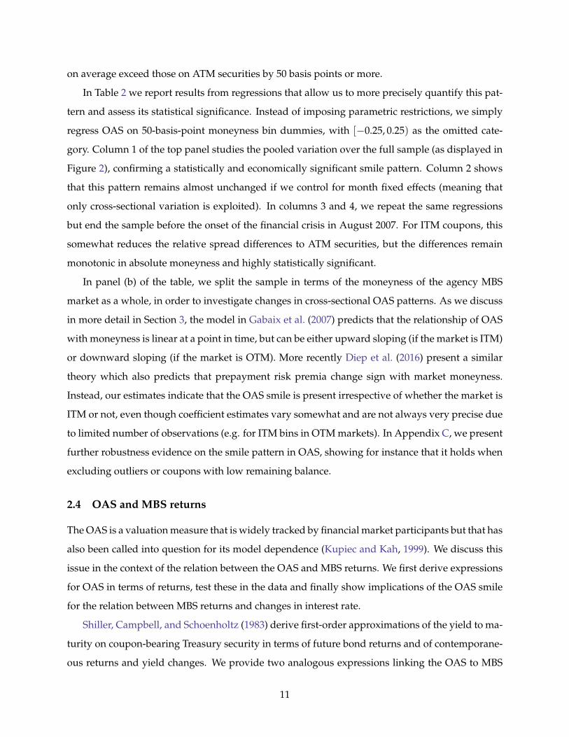
In Table 2 we report results from regressions that allow us to more precisely quantify this pat-

tern and assess its statistical significance. Instead of imposing parametric restrictions, we simply

regress OAS on 50-basis-point moneyness bin dummies, with [−0.25, 0.25) as the omitted cate-

gory. Column 1 of the top panel studies the pooled variation over the full sample (as displayed in

Figure 2), confirming a statistically and economically significant smile pattern. Column 2 shows

that this pattern remains almost unchanged if we control for month fixed effects (meaning that

only cross-sectional variation is exploited). In columns 3 and 4, we repeat the same regressions

but end the sample before the onset of the financial crisis in August 2007. For ITM coupons, this

somewhat reduces the relative spread differences to ATM securities, but the differences remain

monotonic in absolute moneyness and highly statistically significant.

In panel (b) of the table, we split the sample in terms of the moneyness of the agency MBS

market as a whole, in order to investigate changes in cross-sectional OAS patterns. As we discuss

in more detail in Section 3, the model in Gabaix et al. (2007) predicts that the relationship of OAS

with moneyness is linear at a point in time, but can be either upward sloping (if the market is ITM)

or downward sloping (if the market is OTM). More recently Diep et al. (2016) present a similar

theory which also predicts that prepayment risk premia change sign with market moneyness.

Instead, our estimates indicate that the OAS smile is present irrespective of whether the market is

ITM or not, even though coefficient estimates vary somewhat and are not always very precise due

to limited number of observations (e.g. for ITM bins in OTM markets). In Appendix C, we present

further robustness evidence on the smile pattern in OAS, showing for instance that it holds when

excluding outliers or coupons with low remaining balance.

2.4 OAS and MBS returns

The OAS is a valuation measure that is widely tracked by financial market participants but that has

also been called into question for its model dependence (Kupiec and Kah, 1999). We discuss this

issue in the context of the relation between the OAS and MBS returns. We first derive expressions

for OAS in terms of returns, test these in the data and finally show implications of the OAS smile

for the relation between MBS returns and changes in interest rate.

Shiller, Campbell, and Schoenholtz (1983) derive first-order approximations of the yield to ma-

turity on coupon-bearing Treasury security in terms of future bond returns and of contemporane-

ous returns and yield changes. We provide two analogous expressions linking the OAS to MBS

11

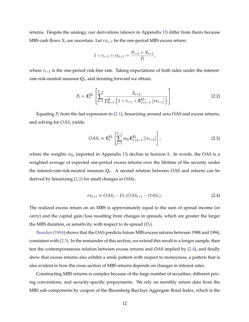
returns. Despite the analogy, our derivations (shown in Appendix D) differ from theirs because

MBS cash flows Xt are uncertain. Let rxt+1 be the one-period MBS excess return:

1 + rt+1 + rxt+1 =Pt+1 + Xt+1

Pt,

where rt+1 is the one-period risk-free rate. Taking expectations of both sides under the interest-

rate-risk-neutral measure Qr, and iterating forward we obtain:

Pt = EQrt

T−t

∑k=1

Xt+k

∏kj=1

(1 + rt+j + E

Qrt+j−1

[rxt+j

]) . (2.2)

Equating Pt from the last expression to (2.1), linearizing around zero OAS and excess returns,

and solving for OAS, yields:

OASt ≈ EQrt

[T−t

∑k=1

wktEQrt+k−1 [rxt+k]

], (2.3)

where the weights wkt (reported in Appendix D) decline in horizon k. In words, the OAS is a

weighted average of expected one-period excess returns over the lifetime of the security under

the interest-rate-risk-neutral measure Qr. A second relation between OAS and returns can be

derived by linearizing (2.2) for small changes in OASt:

rxt+1 ≈ OASt − Dt (OASt+1 −OASt). (2.4)

The realized excess return on an MBS is approximately equal to the sum of spread income (or

carry) and the capital gain/loss resulting from changes in spreads, which are greater the larger

the MBS duration, or sensitivity, with respect to its spread (Dt).

Breeden (1994) shows that the OAS predicts future MBS excess returns between 1988 and 1994,

consistent with (2.3). In the remainder of this section, we extend this result to a longer sample, then

test the contemporaneous relation between excess returns and OAS implied by (2.4), and finally

show that excess returns also exhibit a smile pattern with respect to moneyness, a pattern that is

also evident in how the cross section of MBS returns depends on changes in interest rates.

Constructing MBS returns is complex because of the large number of securities, different pric-

ing conventions, and security-specific prepayments. We rely on monthly return data from the

MBS sub-components by coupon of the Bloomberg Barclays Aggregate Bond Index, which is the

12

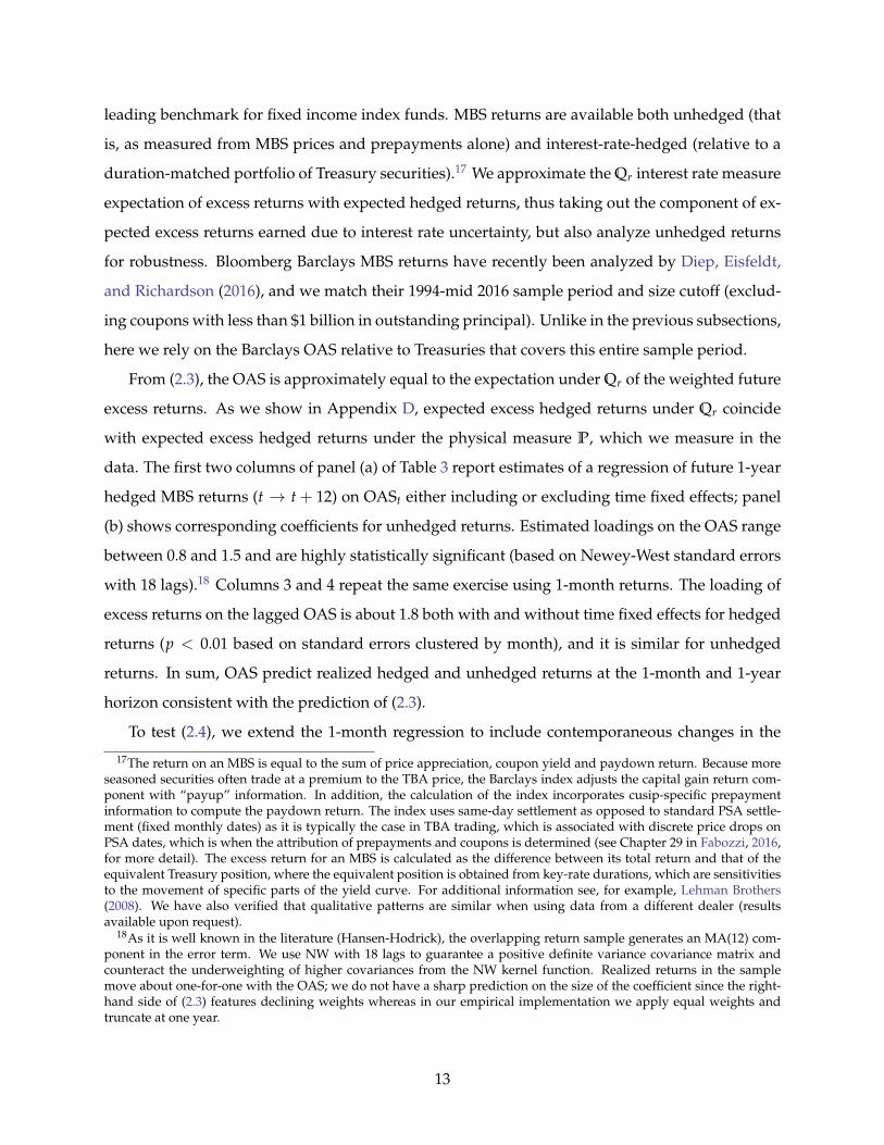
leading benchmark for fixed income index funds. MBS returns are available both unhedged (that

is, as measured from MBS prices and prepayments alone) and interest-rate-hedged (relative to a

duration-matched portfolio of Treasury securities).17 We approximate the Qr interest rate measure

expectation of excess returns with expected hedged returns, thus taking out the component of ex-

pected excess returns earned due to interest rate uncertainty, but also analyze unhedged returns

for robustness. Bloomberg Barclays MBS returns have recently been analyzed by Diep, Eisfeldt,

and Richardson (2016), and we match their 1994-mid 2016 sample period and size cutoff (exclud-

ing coupons with less than $1 billion in outstanding principal). Unlike in the previous subsections,

here we rely on the Barclays OAS relative to Treasuries that covers this entire sample period.

From (2.3), the OAS is approximately equal to the expectation under Qr of the weighted future

excess returns. As we show in Appendix D, expected excess hedged returns under Qr coincide

with expected excess hedged returns under the physical measure P, which we measure in the

data. The first two columns of panel (a) of Table 3 report estimates of a regression of future 1-year

hedged MBS returns (t → t + 12) on OASt either including or excluding time fixed effects; panel

(b) shows corresponding coefficients for unhedged returns. Estimated loadings on the OAS range

between 0.8 and 1.5 and are highly statistically significant (based on Newey-West standard errors

with 18 lags).18 Columns 3 and 4 repeat the same exercise using 1-month returns. The loading of

excess returns on the lagged OAS is about 1.8 both with and without time fixed effects for hedged

returns (p < 0.01 based on standard errors clustered by month), and it is similar for unhedged

returns. In sum, OAS predict realized hedged and unhedged returns at the 1-month and 1-year

horizon consistent with the prediction of (2.3).

To test (2.4), we extend the 1-month regression to include contemporaneous changes in the

17The return on an MBS is equal to the sum of price appreciation, coupon yield and paydown return. Because moreseasoned securities often trade at a premium to the TBA price, the Barclays index adjusts the capital gain return com-ponent with “payup” information. In addition, the calculation of the index incorporates cusip-specific prepaymentinformation to compute the paydown return. The index uses same-day settlement as opposed to standard PSA settle-ment (fixed monthly dates) as it is typically the case in TBA trading, which is associated with discrete price drops onPSA dates, which is when the attribution of prepayments and coupons is determined (see Chapter 29 in Fabozzi, 2016,for more detail). The excess return for an MBS is calculated as the difference between its total return and that of theequivalent Treasury position, where the equivalent position is obtained from key-rate durations, which are sensitivitiesto the movement of specific parts of the yield curve. For additional information see, for example, Lehman Brothers(2008). We have also verified that qualitative patterns are similar when using data from a different dealer (resultsavailable upon request).

18As it is well known in the literature (Hansen-Hodrick), the overlapping return sample generates an MA(12) com-ponent in the error term. We use NW with 18 lags to guarantee a positive definite variance covariance matrix andcounteract the underweighting of higher covariances from the NW kernel function. Realized returns in the samplemove about one-for-one with the OAS; we do not have a sharp prediction on the size of the coefficient since the right-hand side of (2.3) features declining weights whereas in our empirical implementation we apply equal weights andtruncate at one year.

13

OAS. As predicted, the coefficient on the spread change is always negative (p < 0.01) across the

four specifications with point estimates that range between -1.8 and -3.3. The adjusted R2 in the

hedged return regression when omitting time effects exceeds 50%, meaning that changes in OAS

explain much of the realized variation in hedged returns.

A key feature of the cross section of OAS is the smile pattern with respect to a security’s mon-

eyness (see Section 2.3). Figure 3 shows that 1-month excess returns display a similar pattern,

which is also reflected in differential Sharpe ratios (SRs) in the MBS cross section. We compute

(annualized) SRs based on monthly Barclays index returns for portfolios of ITM, ATM and OTM

MBS securities.19 Relative to ATM securities, we find much larger SRs for non-ATM securities: us-

ing unhedged returns (minus the risk-free rate from Ken French’s website), the SR of a long-ITM

(long-OTM) portfolio is 1.86 (1.15) compared to a SR of 0.66 for a long-ATM position. Looking at

hedged returns, we find a similar pattern, although it is more pronounced for ITM securities (ITM

SR = 0.68 ; OTM SR = 0.12; ATM SR = 0.04).

The above analysis established that there is a tight link between realized hedged returns and

changes in OAS: when OAS fall, realized returns tend to be high. In addition, we have docu-

mented a smile-shaped pattern both in expected and realized returns. We now combine these

relations to test an additional prediction about the link between realized returns and changes in

mortgage rates, without relying on OAS directly. Movements in mortgage rates change the mon-

eyness of MBS by moving them along the smile, and the OAS smile predicts an opposite effect of

rate changes on hedged returns depending on whether an MBS is ITM or not. For an OTM MBS,

changes in OAS and changes in rates are positively related, as the MBS moves closer to being

ATM when rates fall. This implies a negative relationship between rate changes and contempora-

neous hedged returns on OTM securities. Conversely, for ITM securities, hedged returns and rate

changes should be positively related.20

Panel (c) of Table 3 shows that as predicted, hedged returns are negatively (positively) related

to changes in mortgage rates for OTM (ITM) securities, irrespective of whether fixed effects are

included or not (columns 1 and 2).21 In columns 3 and 4, we re-estimate this relation in a split

sample based on whether the market as a whole is ITM or not. This allows us to test whether

19We compute the ATM portfolio using the return on the coupon that is closest to zero moneyness in each period,as long as it is not more than 25 basis points ITM or OTM. For the ITM (OTM) portfolio we use the most ITM (OTM)coupon as long as it is at least 100 basis points ITM (OTM).

20The OAS smile implies that OTM securities tend to outperform ITM securities when rates fall, as for example wasthe case following the November 2008 LSAP announcement, discussed in Section 5.3.

21When we add month fixed effects, we can only test whether the relationship between returns and rate changes ismore positive for ITM securities; the uninteracted coefficient on the mortgage rate change is not identified.

14

prepayment risk premia change sign as a function of the market overall moneyness as predicted

by Gabaix et al. (2007) and Diep et al. (2016).22 Contrary to what is implied by these theories,

but consistent with our OAS smile evidence in Section 2.3, we do not find that the relationship

between returns and rate changes flips sign with market moneyness. We return to this issue in the

next section when we present the conceptual framework to analyze the OAS smile.

In sum, our analysis of MBS returns shows that, while model-dependent, the OAS is related

to realized returns, and that a smile pattern is also evident in the cross section of hedged returns.

In the remainder of the paper, we focus on the OAS rather than realized returns, since it is a more

direct and less noisy measure of expected excess returns. Also, as the last part of our analysis

above illustrated, realized returns across securities are affected by changes in realized rates, which

in finite sample could lead to average realized and expected returns having different patterns.

3 Conceptual framework

In this section, we discuss a simple conceptual framework that can be used to understand the

sources of risk premia in the valuation of MBS. Here, we illustrate the main intuition behind

our decomposition of OAS into a prepayment risk premium and a liquidity risk premium under

simple assumptions on the evolution of the interest rate on the loans and the prepayment intensity

function, and discuss the derivation under more general assumptions in Appendix E.

Consider a mortgage pool j with coupon rate cj and remaining principal balance θjt at time t.

The pool prepays with intensity sjt, so that the principal balance evolves (in continuous time) as

dθjt = −sjtθjtdt.

We assume that the prepayment rate sjt is a function of the interest rate incentive cj − r, where r

is the interest rate on new loans, and a vector of parameters γt = (γ1t, γ2t, . . . , γNt)′, which are

uncertain and give rise to non-interest-rate prepayment risk. For ease of notation, we assume here

that the interest rate r is constant, though the derivation in Appendix E shows that the main ex-

pression of interest is the same if we assume that rates follow a diffusion. Suppose the prepayment

22As mentioned earlier, in Gabaix et al. (2007) the relationship of OAS with moneyness is linear and upward slopingif the market is ITM or downward sloping if the market is OTM. This theory thus predicts that in an ITM market, therelationship between hedged returns and mortgage rate changes should be positive for all securities, while in an OTMmarket, the relationship should be negative for all securities.

15

rate is given by

sjt = f(γt, cj − r

).

The parameters γt are time-varying, with normal innovations, so that

dγt = µγdt + σγdZγt,

where Zγt is a standard Brownian motion vector. The other source of uncertainty in the model is

the liquidity of the securities. We assume that, with intensity µt, the whole market experiences a

liquidity event in which a pool j loses a fraction αjt of its market value. Thus αjt should be thought

of as how well the security performs in a “bad” market, similar to Acharya and Pedersen (2005).

Alternatively, αjt could be interpreted as the price impact of a decline in the strength of the agency

guarantee.

Under no-arbitrage there exists a pricing kernel Mt such that the time t price of a future stream

of cash flows Xt+s is

Pt = Et

[∫ +∞

0

Mt+s

MtXt+sds

]. (3.1)

This is analogous to the discrete-time expression for the price of the security (2.1): instead of

taking expectations under the interest-rate-neutral measure Qr and discounting future cash-flows

Xt using the risk-free rate curve shifted by the OAS, we take expectations under the physical

measure and discount using the pricing kernel. Let Rt be the return to holding a claim to the

stream of cash flows Xt, which evolves as

dRt ≡dPt

Pt+

Xt

Ptdt.

The no-arbitrage restriction (3.1) implies that the expected return can be represented as

Et [dRt] = r dt−Et

[dMt

Mt

dPt

Pt

],

where r is the risk-free rate. As shown in Section 2.4, the OAS is, to a first-order approximation,

the lifetime discounted sum of instantaneous risk premia paid to an investor for holding the claim

to X. For tractability, in this conceptual framework, we approximate the OAS by the instantaneous

16

risk premium, denoted rpt, so that

OASt ≈ rpt ≡ −Et

[dMt

Mt

dPt

Pt

].

That is, the risk premium is the covariance between innovations to the price of a security and

innovations to the pricing kernel. To solve for the OAS, denote by πγt the vector of prices of

risks associated with innovations to the prepayment model parameters, and πlt the price of risk

associated with the liquidity shock. As is standard, these risk prices are given by the co-variation

between the innovations to the pricing kernel and the prepayment and liquidity shocks. Since the

liquidity risk is undiversifiable for an investor holding a portfolio of MBS, we have πlt > 1 (see

e.g. Driessen, 2005); we discuss the sign of πγt below.

We show in Appendix E that, with these assumptions, the OAS is given by

OASjt = αjtµt (πlt − 1)− π′γtσγ1

Pjt

∂Pjt

∂γt. (3.2)

Thus, differences in OAS across securities could be the result of (i) differential exposure αj to the

liquidity shock, or (ii) differential price sensitivity to the prepayment parameters, that is, differ-

ential exposure to prepayment risk. Though the expression in eq. (3.2) relies on the particular

assumptions for the dynamics of interest rates, prepayment shocks, and liquidity shocks made in

this section, we show in Appendix E that this decomposition holds more generally.

We can gain further intuition on potential risk premium variation across securities by taking

the first-order approximation of Pjt around the price in the no-uncertainty case,

Pjt = 1 +cj − rr + sjt

, (3.3)

which implies that security j trades at a premium (Pjt > 1) if cj − r > 0 and at a discount (Pjt < 1)

if cj − r < 0. It also shows that for premium securities the price declines as prepayments sjt rise,

while discount securities benefit from faster prepayments.

Using this and applying the chain rule (∂P/∂γ = ∂P/∂s · ∂s/∂γ), we get the following approx-

imate expression for the OAS:

OASjt ≈ αjtµt (πlt − 1) + π′γtσγcj − r(

sjt + cj) (

sjt + r) ∂sjt

∂γt. (3.4)

17

We can use this expression to understand the conditions under which prepayment risk can lead

to the OAS smile. We consider three stylized representations of borrowers’ prepayment behavior.

In each case, sj corresponds to the expected prepayment speed on security j.

Case 1: sjt = sj + γ1tβ j. This is essentially the framework studied by Gabaix et al. (2007). Each

pool has a constant exposure β j to a single market-wide prepayment shock γ1. Under this func-

tional form, the OASjt in (3.2) will be a linear function of moneyness cj − r (regardless of the sign

of the risk price πγ1t ). This case is therefore inconsistent with the OAS smile.

Case 2: sjt = sj + γ1t(cj− rt). Like in the previous case, a single factor drives prepayment behav-

ior, but the security’s exposure to the prepayment shock now depends on its moneyness, which

varies over time.23 This functional form implies that when ITM securities prepay faster than ex-

pected (a positive shock to γ1), OTM securities prepay slower than expected. This may arise be-

cause of mortgage originators’ capacity constraints in (larger than expected) refinancing waves.24

It is easy to see from (3.2) that this case would lead the OAS to be quadratic in cj − r (the risk price

πγ1t is positive in this case, since every security has a positive exposure to γ1), and therefore could

rationalize the OAS smile.

Case 3: sjt = sj + γ1t1cj<r + γ2t1cj≥r. In this multi-factor formulation, OTM and ITM prepay-

ments are driven by different shocks (which for simplicity we assume to be orthogonal). For

instance, γ1t might represent the pace of housing turnover while γ2t might be the effective cost of

mortgage refinancing (which varies with underwriting standards and market competitiveness). In

equilibrium, the signs of the prices of risk are determined by the average exposure of the represen-

tative investor. Holding a portfolio of ITM and OTM securities, this investor will have a negative

exposure to γ1t risk (since OTM securities benefit from fast prepayment) and a positive exposure

to γ2t risk (since the price of ITM securities declines with faster prepayments). Thus πγ1,t < 0 and

πγ2,t > 0, resulting in a positive OAS for both ITM and OTM securities and a (v-shaped) OAS

smile.

23γ1 > 0 because in practice prepayments are a non-decreasing function of the incentive to refinance.24When capacity is tight, mortgage originators may be less willing to originate purchase loans (which are more labor

intensive), and they may reduce marketing effort targeted at OTM borrowers (for instance, to induce them to cashout home equity by refinancing their loan). Fuster et al. (2017) show that originators’ pricing margins are stronglycorrelated with mortgage application volume, consistent with the presence of capacity constraints.

18

In sum, the OAS displays a smile pattern in moneyness if prepayments are driven by the

specification in case 2 or 3, but not in the single-factor representation of case 1. More generally,

prepayment risk premia can explain the OAS smile whenever OTM securities are not a hedge for

ITM pools (as they would be in case 1).25 To separate liquidity and prepayment risk premia, in the

next section we provide a method to identify a “prepayment-risk-neutral OAS,” denoted OASQ,

as the spread that only reflects liquidity risk:

OASQjt = αjtµt (πlt − 1) . (3.5)

The prepayment risk premium paid to the investor is then just the difference between the OAS

and OASQ.

4 Pricing model: Decomposing the OAS

In this section, we propose a method to decompose the “standard” OAS into a prepayment risk

premium component and a remaining risk premium (OASQ). We then implement this method

using a pricing model, which consists of an interest rate and a prepayment component. In contrast

to standard approaches, such as Stanton (1995) or practitioner models, we employ information

from stripped MBS to identify a market-implied prepayment function and the contribution of

prepayment risk to the OAS.

4.1 Identification of OASQ

As discussed in the Section 2, the OAS only accounts for interest rate uncertainty (and only interest

rates are simulated in empirical pricing models) and ignores other sources of prepayment risk,

such as uncertainty about house prices or lending standards. In this section we propose a method

to identify a risk-neutral prepayment function obtained from market prices, then compute an OAS

using this function (OASQ) and finally obtain the contribution of prepayment risk to the OAS.

Following the credit risk literature (e.g. Driessen, 2005), we assume that the market-implied

risk-neutral (“Q”) prepayment function is a multiple Λ of the physical (“P”) one. We allow the

multiplier Λ to be pool-specific to account for differences in pools’ sensitivities to non-interest rate

25This is also pointed out by Levin and Davidson (2005), who note that “[a] single-dimensional risk analysis wouldallow for hedging prepayment risk by combining premium MBS and discount MBS, a strategy any experienced traderknows would fail.”

19

sources of prepayment risk. The multiplier Λ is also allowed to vary over time. Because of the

large number of parameters that characterize the P prepayment function, we make the assumption

that the Q prepayment function is a multiple of the P prepayment function for parsimony. As we

discuss below, our key finding that the smile pattern in OAS is due to prepayment risk premia

while OASQ is flat with respect to moneyness is preserved in an alternative framework where the

Q prepayment is estimated from the cross section of MBS prices only.

Pricing information on a standard pass-through MBS alone is insufficient to identify Λ, be-

cause a single observable (the price) can only determine one unknown (the spread) in the pricing

model, leaving Λ unidentified. To resolve this identification problem, we use additional pricing

information from “stripped” MBS, which separate cash flows from pass-through securities into

an interest component (“interest only” or IO strip) and a principal component (“principal only”

or PO strip). Cash flows of these strips depend on the same underlying prepayment path and

therefore face the same prepayment risk, but are exposed to it in opposite ways, as illustrated in

Figure 4. As prepayment rates increase (top to bottom panel), total interest payments shrink (since

interest payments accrue only as long as the principal is outstanding) and thus the value of the IO

strip declines. Conversely, principal cash flows (the gray areas) are received sooner, and therefore

the value of the PO strip increases.

We exploit the differential exposure of the two strips to prepayments to identify OASQ and Λ,

as illustrated graphically in the example of Figure 5. At Λ = 1, the physical prepayment speed,

the OAS on the IO strip (shown in black) is about 200 basis points and the OAS on the PO (shown

in gray) is about zero. As Λ increases, the OAS on the IO declines while the spread on the PO

increases because of their opposite sensitivities to prepayments. The sensitivity of the OAS on the

pass-through (“recombined” as the sum of IO and PO) is also negative (red line), because in this

example it is assumed to be a premium security and so its price declines with faster prepayments.

For each IO/PO pair, we identify Λ as the crossing of the OAS IO and PO schedules at the

point where the residual risk premium (OASQ) on the two strips is equalized.26 By the law of one

price, the residual risk premium on the pass-through will also be equalized at this point; thus,

the OAS schedule on the pass-through intersects the other two schedules at the same point. The

difference between the OAS on the pass-through at the physical prepayment speed (OAS) and

at the market-implied one (OASQ) is then equal to the prepayment risk premium paid on the

26MBS market participants sometimes calculate “break-even multiples” similar to our Λ but, to our knowledge, donot seem to track them systematically as measures of risk prices.

20

pass-through. More formally:

Proposition 4.1. Consider a complete probability space (Ω,F , P), generated by an N-dimensional Brow-

nian motion Zt, that generate interest rate risk and non-interest-rate prepayment risk, and a Poisson process

Jt, that generates liquidity risk for the market. Assume that all securities written on pool j lose the same

fraction αjt of their market value in the case of a jump occurring at date t, so that the IO strip and the

PO strip on a pool j have equal exposures to non-prepayment sources of risk. Then, by no arbitrage, when

expectations are calculated under the measure risk-neutral with respect to all Brownian shocks, Qr,γ, the

remaining risk premia are equalized on the strips and recombined pass-through, so that

OASQIO,j = OASQ

PO,j = OASQj .

The OASQk,j on security of type k ∈ IO, PO, pass-through is defined implicitly by

Pk,jt = EQr,γt

[∫ +∞

0exp

(−∫ s

0

[rt+u + OASQ

k,jt+u

]du)

dXk,jt+s

],

where Pk,jt is the market price of the security,

dXk,jt+s

is the stream of cash-flows earned by the security,

and rt is the risk-free rate, which evolves as a function of Zt.

Proof. See the derivation of the OASQ in Appendix E.

We then define the prepayment risk premium component in the OAS as follows:

Definition 4.1. The prepayment risk premium on a pass-through security (consisting of the combination

of an IO and PO strip on the same underlying pool) is equal to OAS−OASQ.

We apply this method to each IO/PO pair in our sample, thereby identifying pool- and date-

specific Λ and OASQ. This allows us to study time-series and cross-sectional variation in the

OASQ without imposing parametric assumptions and we can thus remain agnostic as to whether

prepayment risk or other risks are the source of the OAS smile.27 Notice that while the above

discussion (and the theoretical derivations in Appendix E) has emphasized the case of prepayment

risk premia due to non-interest rate factors, our empirical setting also subsumes the possibility of

a prepayment event risk premium (which by itself would lead to date-specific Λ).

27An alternative way to identify Λ would be to assume that the OAS reflects only prepayment risk. With this ap-proach, Levin and Davidson (2005) obtain a Q prepayment function by equalizing the OAS (relative to agency debt)on all pass-through coupons to zero. By construction, both the time-series and cross-sectional variation in the OAS willthen be the result of variation in prepayment risk.

21

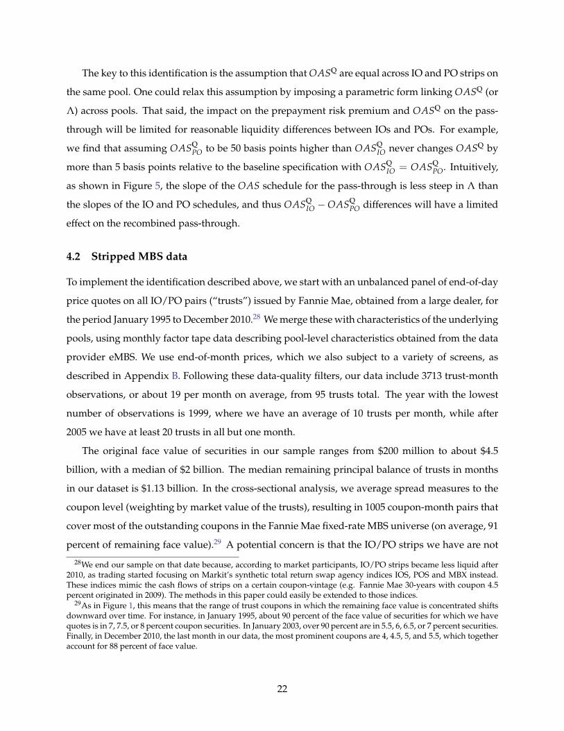
The key to this identification is the assumption that OASQ are equal across IO and PO strips on

the same pool. One could relax this assumption by imposing a parametric form linking OASQ (or

Λ) across pools. That said, the impact on the prepayment risk premium and OASQ on the pass-

through will be limited for reasonable liquidity differences between IOs and POs. For example,

we find that assuming OASQPO to be 50 basis points higher than OASQ

IO never changes OASQ by

more than 5 basis points relative to the baseline specification with OASQIO = OASQ

PO. Intuitively,

as shown in Figure 5, the slope of the OAS schedule for the pass-through is less steep in Λ than

the slopes of the IO and PO schedules, and thus OASQIO −OASQ

PO differences will have a limited

effect on the recombined pass-through.

4.2 Stripped MBS data

To implement the identification described above, we start with an unbalanced panel of end-of-day

price quotes on all IO/PO pairs (“trusts”) issued by Fannie Mae, obtained from a large dealer, for

the period January 1995 to December 2010.28 We merge these with characteristics of the underlying

pools, using monthly factor tape data describing pool-level characteristics obtained from the data

provider eMBS. We use end-of-month prices, which we also subject to a variety of screens, as

described in Appendix B. Following these data-quality filters, our data include 3713 trust-month

observations, or about 19 per month on average, from 95 trusts total. The year with the lowest

number of observations is 1999, where we have an average of 10 trusts per month, while after

2005 we have at least 20 trusts in all but one month.

The original face value of securities in our sample ranges from $200 million to about $4.5

billion, with a median of $2 billion. The median remaining principal balance of trusts in months

in our dataset is $1.13 billion. In the cross-sectional analysis, we average spread measures to the

coupon level (weighting by market value of the trusts), resulting in 1005 coupon-month pairs that

cover most of the outstanding coupons in the Fannie Mae fixed-rate MBS universe (on average, 91

percent of remaining face value).29 A potential concern is that the IO/PO strips we have are not

28We end our sample on that date because, according to market participants, IO/PO strips became less liquid after2010, as trading started focusing on Markit’s synthetic total return swap agency indices IOS, POS and MBX instead.These indices mimic the cash flows of strips on a certain coupon-vintage (e.g. Fannie Mae 30-years with coupon 4.5percent originated in 2009). The methods in this paper could easily be extended to those indices.

29As in Figure 1, this means that the range of trust coupons in which the remaining face value is concentrated shiftsdownward over time. For instance, in January 1995, about 90 percent of the face value of securities for which we havequotes is in 7, 7.5, or 8 percent coupon securities. In January 2003, over 90 percent are in 5.5, 6, 6.5, or 7 percent securities.Finally, in December 2010, the last month in our data, the most prominent coupons are 4, 4.5, 5, and 5.5, which togetheraccount for 88 percent of face value.

22

necessarily representative of securities traded in the TBA market, to which we are comparing our

model output. As we will see, however, we obtain similar spread patterns based on IO/PO prices,

both in the time series and cross section. One advantage of the stripped MBS that we are using

relative to TBAs, which trade on a forward “cheapest-to-deliver” basis, is that we do not need to

make assumptions about the characteristics of the security.

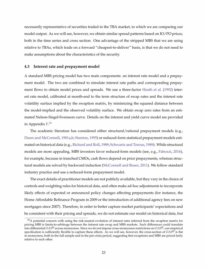
4.3 Interest rate and prepayment model

A standard MBS pricing model has two main components: an interest rate model and a prepay-

ment model. The two are combined to simulate interest rate paths and corresponding prepay-

ment flows to obtain model prices and spreads. We use a three-factor Heath et al. (1992) inter-

est rate model, calibrated at month-end to the term structure of swap rates and the interest rate

volatility surface implied by the swaption matrix, by minimizing the squared distance between

the model-implied and the observed volatility surface. We obtain swap zero rates from an esti-

mated Nelson-Siegel-Svensson curve. Details on the interest and yield curve model are provided

in Appendix F.30

The academic literature has considered either structural/rational prepayment models (e.g.,

Dunn and McConnell, 1981a,b; Stanton, 1995) or reduced-form statistical prepayment models esti-

mated on historical data (e.g., Richard and Roll, 1989; Schwartz and Torous, 1989). While structural

models are more appealing, MBS investors favor reduced-form models (see, e.g., Fabozzi, 2016),

for example, because in tranched CMOs, cash flows depend on prior prepayments, whereas struc-

tural models are solved by backward induction (McConnell and Buser, 2011). We follow standard

industry practice and use a reduced-form prepayment model.

The exact details of practitioner models are not publicly available, but they vary in the choice of

controls and weighting rules for historical data, and often make ad-hoc adjustments to incorporate

likely effects of expected or announced policy changes affecting prepayments (for instance, the

Home Affordable Refinance Program in 2009 or the introduction of additional agency fees on new

mortgages since 2007). Therefore, in order to better capture market participants’ expectations and

be consistent with their pricing and spreads, we do not estimate our model on historical data, but

30A potential concern with using the risk-neutral evolution of interest rates inferred from the swaption matrix forpricing MBS is limits-to-arbitrage between the interest rate swap and MBS markets. Such differences could translateinto differential OASQ across moneyness. Since we do not impose cross-moneyness restrictions on OASQ, our empiricalspecification is sufficiently flexible to capture these effects. As we will see, however, the cross-section of OASQ is flatin moneyness, both in the full sample and in the pre-crisis period, suggesting that swaptions and MBS are priced fairlyrelative to each other.

23

instead extract prepayment model parameters from a survey of dealer models from Bloomberg

LP. In these surveys, major MBS dealers provide their model forecasts of long-term prepayment

speeds under different constant interest rate scenarios (with a range of +/- 300 basis points relative

to current rates).31 Carlin et al. (2014) use these data to study the pricing effects of investors’

disagreement measured from “raw” long-run prepayment projections. We, instead, extract model

parameters of a monthly prepayment function by explicitly accounting for loan amortization, the

path of interest rates, and changes in a pool’s borrower composition.

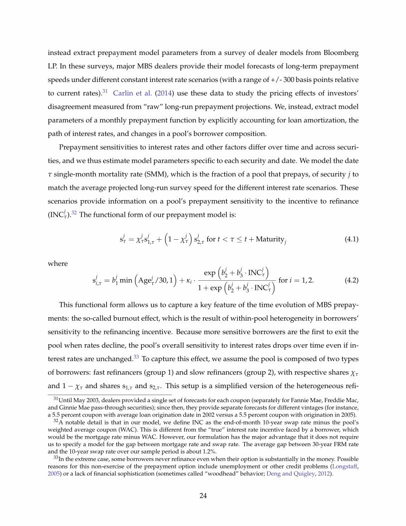
Prepayment sensitivities to interest rates and other factors differ over time and across securi-

ties, and we thus estimate model parameters specific to each security and date. We model the date

τ single-month mortality rate (SMM), which is the fraction of a pool that prepays, of security j to

match the average projected long-run survey speed for the different interest rate scenarios. These

scenarios provide information on a pool’s prepayment sensitivity to the incentive to refinance

(INCjτ).32 The functional form of our prepayment model is:

sjτ = χ

jτsj

1,τ +(

1− χjτ

)sj

2,τ for t < τ ≤ t + Maturityj (4.1)

where

sji,τ = bj

1 min(

Agejτ/30, 1

)+ κi ·

exp(

bj2 + bj

3 · INCjτ

)1 + exp

(bj

2 + bj3 · INCj

τ

) for i = 1, 2. (4.2)

This functional form allows us to capture a key feature of the time evolution of MBS prepay-

ments: the so-called burnout effect, which is the result of within-pool heterogeneity in borrowers’

sensitivity to the refinancing incentive. Because more sensitive borrowers are the first to exit the

pool when rates decline, the pool’s overall sensitivity to interest rates drops over time even if in-

terest rates are unchanged.33 To capture this effect, we assume the pool is composed of two types

of borrowers: fast refinancers (group 1) and slow refinancers (group 2), with respective shares χτ

and 1− χτ and shares s1,τ and s2,τ. This setup is a simplified version of the heterogeneous refi-

31Until May 2003, dealers provided a single set of forecasts for each coupon (separately for Fannie Mae, Freddie Mac,and Ginnie Mae pass-through securities); since then, they provide separate forecasts for different vintages (for instance,a 5.5 percent coupon with average loan origination date in 2002 versus a 5.5 percent coupon with origination in 2005).

32A notable detail is that in our model, we define INC as the end-of-month 10-year swap rate minus the pool’sweighted average coupon (WAC). This is different from the “true” interest rate incentive faced by a borrower, whichwould be the mortgage rate minus WAC. However, our formulation has the major advantage that it does not requireus to specify a model for the gap between mortgage rate and swap rate. The average gap between 30-year FRM rateand the 10-year swap rate over our sample period is about 1.2%.

33In the extreme case, some borrowers never refinance even when their option is substantially in the money. Possiblereasons for this non-exercise of the prepayment option include unemployment or other credit problems (Longstaff,2005) or a lack of financial sophistication (sometimes called “woodhead” behavior; Deng and Quigley, 2012).

24

nancing cost framework of Stanton (1995). As shown in equation (4.1), total pool prepayments are

share-weighted averages of each group’s prepayment speed. Each group’s prepayment depends

on two components. The first, which is identical to both groups, is governed by b1 and accounts

for non-rate-driven prepayments, such as housing turnover. Because relocations are less likely

to occur for new loans, we assume a seasoning of this effect using the industry-standard “PSA”

assumption, which posits that prepayments increase for the first 30 months in the life of a security

and are constant thereafter. The second component captures the rate-driven prepayments due to

refinancing. This is modeled as a logistic function of the rate incentive (INC), with a sensitivity κi

that differs across the two groups: κ1 > κ2. Since group 1 prepays faster, χτ declines over time

in the pool. This changing composition, which we track in the estimation, captures the burnout

effect. We provide more detail on the prepayment model and parameter estimation in Appendix F.

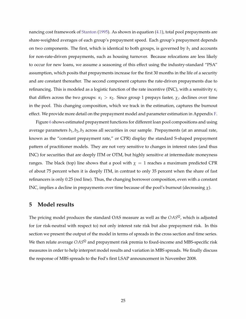
Figure 6 shows estimated prepayment functions for different loan pool compositions and using

average parameters b1, b2, b3 across all securities in our sample. Prepayments (at an annual rate,

known as the “constant prepayment rate,” or CPR) display the standard S-shaped prepayment

pattern of practitioner models. They are not very sensitive to changes in interest rates (and thus

INC) for securities that are deeply ITM or OTM, but highly sensitive at intermediate moneyness

ranges. The black (top) line shows that a pool with χ = 1 reaches a maximum predicted CPR

of about 75 percent when it is deeply ITM, in contrast to only 35 percent when the share of fast

refinancers is only 0.25 (red line). Thus, the changing borrower composition, even with a constant

INC, implies a decline in prepayments over time because of the pool’s burnout (decreasing χ).

5 Model results

The pricing model produces the standard OAS measure as well as the OASQ, which is adjusted

for (or risk-neutral with respect to) not only interest rate risk but also prepayment risk. In this

section we present the output of the model in terms of spreads in the cross section and time series.

We then relate average OASQ and prepayment risk premia to fixed-income and MBS-specific risk

measures in order to help interpret model results and variation in MBS spreads. We finally discuss

the response of MBS spreads to the Fed’s first LSAP announcement in November 2008.

25

5.1 OAS smile

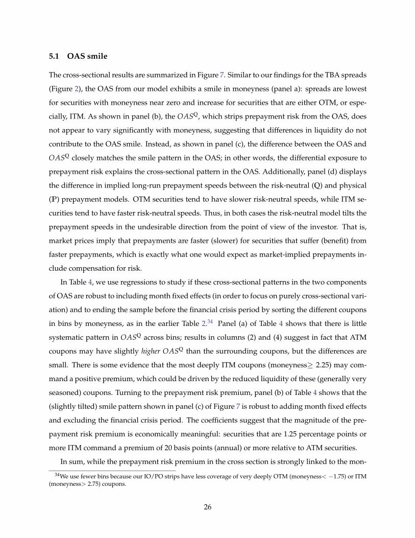
The cross-sectional results are summarized in Figure 7. Similar to our findings for the TBA spreads

(Figure 2), the OAS from our model exhibits a smile in moneyness (panel a): spreads are lowest

for securities with moneyness near zero and increase for securities that are either OTM, or espe-

cially, ITM. As shown in panel (b), the OASQ, which strips prepayment risk from the OAS, does

not appear to vary significantly with moneyness, suggesting that differences in liquidity do not

contribute to the OAS smile. Instead, as shown in panel (c), the difference between the OAS and

OASQ closely matches the smile pattern in the OAS; in other words, the differential exposure to

prepayment risk explains the cross-sectional pattern in the OAS. Additionally, panel (d) displays

the difference in implied long-run prepayment speeds between the risk-neutral (Q) and physical

(P) prepayment models. OTM securities tend to have slower risk-neutral speeds, while ITM se-

curities tend to have faster risk-neutral speeds. Thus, in both cases the risk-neutral model tilts the

prepayment speeds in the undesirable direction from the point of view of the investor. That is,

market prices imply that prepayments are faster (slower) for securities that suffer (benefit) from

faster prepayments, which is exactly what one would expect as market-implied prepayments in-

clude compensation for risk.

In Table 4, we use regressions to study if these cross-sectional patterns in the two components

of OAS are robust to including month fixed effects (in order to focus on purely cross-sectional vari-

ation) and to ending the sample before the financial crisis period by sorting the different coupons

in bins by moneyness, as in the earlier Table 2.34 Panel (a) of Table 4 shows that there is little

systematic pattern in OASQ across bins; results in columns (2) and (4) suggest in fact that ATM

coupons may have slightly higher OASQ than the surrounding coupons, but the differences are

small. There is some evidence that the most deeply ITM coupons (moneyness≥ 2.25) may com-

mand a positive premium, which could be driven by the reduced liquidity of these (generally very

seasoned) coupons. Turning to the prepayment risk premium, panel (b) of Table 4 shows that the

(slightly tilted) smile pattern shown in panel (c) of Figure 7 is robust to adding month fixed effects

and excluding the financial crisis period. The coefficients suggest that the magnitude of the pre-

payment risk premium is economically meaningful: securities that are 1.25 percentage points or

more ITM command a premium of 20 basis points (annual) or more relative to ATM securities.

In sum, while the prepayment risk premium in the cross section is strongly linked to the mon-

34We use fewer bins because our IO/PO strips have less coverage of very deeply OTM (moneyness< −1.75) or ITM(moneyness> 2.75) coupons.

26

eyness of the securities, we find little evidence that this is also the case for the remaining risk pre-

mium (OASQ), suggesting that differential liquidity across coupons is likely not a major driver of

cross-sectional variation in spreads (except perhaps for the most deeply ITM securities). Instead,

the smile in prepayment risk premia suggests that both ITM and OTM securities earn positive

compensation for prepayment risk, consistent with them not being hedges for one another. Going

back to our conceptual framework, this would arise if either a single shock drives prepayments

but with opposite effects on ITM and OTM securities (case 2), or, perhaps more realistically, if

OTM and ITM securities were subject to distinct but independent shocks (case 3). For instance,

OTM prepayments could be primarily driven by housing-relocation shocks, such as house prices,

whereas variation in ITM prepayments could be due to shocks to refinancing activity.

Though Table 4 shows that the cross-sectional patterns in the two components of OAS are

robust to including month fixed effects and to ending the sample in 2007, a potential concern is

whether these results could be due to potential misspecification of the risk-neutral prepayment

function as a multiple of the physical prepayment function. Note that the multiple Λ is security

and date specific, so that our estimate of the Q prepayment function is semi-parametric and allows

us to capture risk premia with the least restrictive prior assumptions. Nevertheless, in Appendix G

we explore an alternative identification methodology that estimates the risk-neutral prepayment

function directly from IO/PO prices only, without requiring us to start with a P prepayment func-

tion. While this alternative approach does not allow the estimation of prepayment risk premia, it

confirms this section’s finding that the OASQ does not vary systematically with moneyness.

5.2 Time-series variation

We now turn to the variation in the average OAS in the time series. As in Section 2, we construct

a market value-weighted index of our model-implied OAS.35 Comparing the OAS in Figure 8 to

the corresponding series in panel (a) of Figure 2 confirms that our model output is close to its

dealer counterparts. As in these models, the level of the average OAS is generally close to zero,

but increases in periods of market stress. Further, our pricing model finds the difference between

OAS and OASQ to be small and the two series to tightly co-move, meaning that much of the OAS

variation results from changes in OASQ (gray line). Thus, although it is an important determinant

of the cross-sectional variation in spreads, prepayment risk does not appear to be the dominant

35We do this by first averaging spreads across trusts within a coupon (weighting each trust by its market value, givenby its remaining principal balance times the sum of the prices of its IO and PO strips). Then, we average across couponsin a given month (weighting each coupon by its market value based on TBA prices, as in Section 2.2).

27

driver of the OAS time-series variation. Indeed as shown in Figure 1, the share of deeply OTM or

ITM securities, which earn most compensation for prepayment risk, is limited; this arises because

most securities are close to ATM when issued.36 However, prepayment risk in the MBS universe

can be significant when mortgage rates move sharply, as in early 1998, the summer of 2003, and in

2009 and 2010 as mortgage rates reached historic lows and the gap between the average OAS and

OASQ widened.

We next investigate the determinants of the time-series variation in OAS, and in particular its

two components: OASQ and the prepayment risk premium. Table 5 shows results from monthly

regressions of the OAS, and its components, on mortgage-specific risk factors, such as spreads

on agency debt (or debentures) relative to swaps, agency MBS issuance (normalized by broker-

dealer book equity, and subtracting Fed MBS purchases in 2009 and 2010), the average squared

moneyness of the MBS universe, as well as dealer disagreement about future prepayment speeds,

which Carlin et al. (2014) find to be significant predictors of MBS returns.37 We construct our

disagreement measure in the same way as Carlin et al. (2014), but based on the Bloomberg surveys

on Fannie Mae prepayment speeds that we already use for the physical prepayment model (while

Carlin et al. instead use forecasts of Ginnie Mae prepayments). We also include the credit spread,

which was the main economically and statistically significant factor in the TBA analysis in Table 1.

We find that average OASQ are related to spreads on (unsecured) agency debentures. As noted

earlier, agency MBS are typically perceived as being free of credit risk, but since the government

guarantee on securities issued by Fannie Mae is only implicit, investors’ perceptions of this guar-

antee (along with the perceived credit risk of agencies) may change over time and thus affect both

spreads on agency debt and MBS. In particular, both OASQ and agency debt spreads increased in

the fall of 2008, when Fannie Mae and Freddie Mac were placed in conservatorship by the U.S.

Treasury. The spreads on MBS and agency debt do, however, also co-move earlier in the sample,

pointing to other common factors such as liquidity and funding costs of these securities.38

36After issuance, the moneyness of securities fluctuates as a function of interest rates and the remaining balancedeclines with prepayments, lowering the importance of older issues on a value-weighted basis.

37Agency debenture yields and swap yields come from Barclays; agency MBS issuance is from eMBS; Fed MBSpurchases from the https://www.federalreserve.gov/regreform/reform-mbs.htm; and broker-dealer equity fromTable L.130 in the Flow of Funds (interpolated linearly between quarter-ends).

38The spread between Fannie Mae debentures and Treasury bonds of equal maturity fell following the conservator-ship announcement, but then substantially increased through the end of 2008. Since there should have been essentiallyno difference in the strength of the debt guarantee between debentures and Treasuries at that point, and since the spreadwidening was stronger for shorter maturity bonds, Krishnamurthy (2010) argues that this reflects a flight to liquidity.In line with this interpretation, our OASQ also reaches substantially higher levels in October compared to August 2008,despite the reduction in credit risk to investors.

28

Credit spreads (Baa-Aaa) continue to be significantly related to OAS, mostly through OASQ

rather than the prepayment risk component. The sensitivity of OASQ to credit spreads suggests

common pricing factors in the MBS and credit markets, such as limited risk-bearing capacity of

financial intermediaries (see, for example, Shleifer and Vishny, 1997; Duffie, 2010; Gabaix et al.,

2007; He and Krishnamurthy, 2013). In these models, financial intermediaries are marginal in-

vestors in risky assets; when their financial constraints bind, their effective risk aversion increases,

raising risk premia in all markets. Thus, when the supply of risky assets relative to intermedi-

aries’ capital decreases, financial constraints are relaxed, lowering required risk compensation. In

line with these predictions, we find that higher supply of MBS, measured by issuance relative to

mark-to-market equity of brokers and dealers, also positively correlates with average OASQ.39 We

explore this channel further in the next section, where we study the effects of Fed MBS purchases,

which absorb supply in the hands of investors, on the OAS and its components.

Disagreement about future prepayments (for given rates) is positively related to the prepay-

ment risk premium, in line with the findings of Carlin et al. (2014); however, the economic magni-

tude of the coefficient is relatively small. Finally, as previously discussed, the OAS smile implies

that spreads, and in particular their prepayment risk component, are largest for deeply OTM and

ITM securities. This suggests that when the market-value weighted moneyness is either very pos-

itive or very negative, the average OAS and prepayment risk premium should be large. In line

with this prediction, we find average squared moneyness to be positively related to the average

prepayment risk premium.

5.3 Interpreting the OAS response to the Fed’s LSAPs

As discussed above, MBS spreads are positively related to MBS supply, a finding that is consis-

tent with intermediary asset pricing models with limited risk-bearing capacity. In this section we

provide additional evidence on this channel by focusing on the Fed’s large-scale asset purchase

(LSAP) program. The program has entailed an unprecedented shift in the composition of the MBS

investor base as the Fed now holds more than a quarter of the total agency MBS universe—up

from nothing prior to the financial crisis. We decompose spreads using our pricing model and

show how our model can explain the divergence in OAS across different coupons following the

39As noted above, we net out monthly Fed purchases by settlement month over 2009-10 from new issuance to moreproperly measure fluctuations in net supply that is absorbed by investors. Relatedly, GSEs’ conservatorship agreementshave required them to divest their portfolios since 2010, a process that would affect net supply in the hands of otherinvestors. However, during the first round of LSAPs, which we focus on, changes in GSE holdings of agency MBS werequite small relative to Fed purchases and issuance.

29

initial announcement of the program.

We focus on spread movements after November 25, 2008, when the Fed announced its first

round of purchases of up to $500 billion in agency MBS.40 Based on the current coupon MBS, which

is the focus of much of the research on this topic—with the important exception of Krishnamurthy

and Vissing-Jorgensen (2013) which we discuss in the paper’s conclusion—the announcement had

a substantial effect on the MBS market (see, e.g., Gagnon et al. 2011 or Hancock and Passmore 2011;

Stroebel and Taylor 2012 are more skeptical). According to different dealer models, the current

coupon OAS, which had been at record levels of 75–100 basis points over October and November

2008, fell 30–40 basis points on the day of the announcement, and stayed around the lower level

afterwards. Consistent with the decline in secondary MBS spreads and yields, headline 30-year

FRM rates dropped nearly a full percentage point between mid-November and year-end 2008.

Spread movements on the current coupon MBS alone hide significant heterogeneity across the

coupon stack, as evidenced by the series in Figure 9, which are median spreads across dealer

models (the same used in Section 2) for the four main coupons traded at that time. OAS that were

all at similarly elevated levels in the fall of 2008 diverged following the announcement. Between

October and November 2008, spreads on low coupons (4.5 and 5) fell, while, over the same period,

those on higher coupons were little changed and then even widened through the end of December.

Since high coupons represent the majority of outstanding MBS, this implies that, for specialized

investors in this market, the recapitalization effect of monetary policy described in Brunnermeier

and Sannikov (2012) was limited.

The earlier findings from our model suggest two potentially countervailing effects of Fed MBS

purchases on OAS. On the one hand, Fed purchases reduce MBS supply to be absorbed by risk-

sensitive investors, thereby reducing the required risk premium on all MBS (through OASQ).41

On the other hand, movements in mortgage rates associated with such purchases alter securities’

moneynesses, shifting the OAS along the smile and changing the prepayment risk premium.

The results from our model are shown in the bottom panel of Figure 10. First, OAS movements

(in black) for IO/PO pass-throughs are similar to the TBA ones.42 In terms of the MBS supply

40The Fed also announced that it would purchase up to $100 billion in agency debt. The purchases began in earlyJanuary 2009. The program was then extended in March 2009, when it was announced that an additional $750bn inagency MBS, $100bn in agency debt, and $300bn in long-term Treasuries would be purchased over the following year.

41Over several months in early 2009, monthly Fed MBS purchases were absorbing essentially all new agency MBSissuance.

42The strips we have available do not necessarily have the same characteristics as what the dealers assume to becheapest-to-deliver in TBA trades; therefore, our OAS levels do not exactly line up with theirs for all coupons in allmonths. Nevertheless, patterns are very similar, especially in changes.

30

effect, we discussed above how the OASQ component is flat across coupons and declines with a

reduction in MBS supply. Consistent with this, we find that the OASQ evolves similarly for the

4.5, 5, and 5.5 coupons. For the 6 coupon, OASQ increases in November and December, before

dropping toward the level of the other coupons in January as actual LSAP purchases begin. The

OASQ effect thus suggests that the LSAP program lowered non-prepayment risk premia across

the coupon stack.43

The cross-coupon “homogeneous” OASQ impact of the Fed’s policy is, however, masked by

changes in the prepayment risk premia that vary with MBS moneyness, shown in the top panel

of Figure 10. The 4.5 starts out OTM and moves ATM as mortgage rates drop, while the 5.5

and 6, which are around ATM in October, move quite deeply ITM. Based on the OAS smile, the

4.5 should command a prepayment risk premium prior to November and the 5.5 and 6 coupons

afterward. The bottom panel shows that this is indeed the case: the narrowing in the gap between

the black and gray lines means that the decrease in the OAS of the 4.5 coupon is in part due to the

decrease in its prepayment risk exposure following the drop in rates. In contrast, the prepayment

risk premia on the 5.5 and 6 coupons are high from December onward as they move deeply ITM

and are more sensitive to prepayment risk.

In sum, increases in the moneyness of high coupons following the November 2008 LSAP an-

nouncement led to an increase in their prepayment risk premium, which explains why their OAS

did not fall, even though OASQ declines across the coupon stack as the Fed started absorbing MBS

supply. We discuss the policy implications of these results below.

6 Conclusions

Our pricing model has two main implications. In the cross section, risk premia associated with

non-interest-rate prepayment factors explain the OAS smile, which is the fact that OAS tend to be

lower for at-the-money MBS than for others. In the time series, the model implies that the average

OAS is primarily driven by non-prepayment risk factors linked to credit spreads, MBS supply, and

spreads on other agency debt. These results suggest that risk-bearing capacity of MBS investors,

and the liquidity and default risk of agency securities, drive aggregate spread variation and are

important determinants of homebuyers’ funding costs.

43In addition to the supply effect, the Fed announcement may also have strengthened the perceived governmentbacking of Fannie Mae and Freddie Mac and improved the liquidity of agency securities (Hancock and Passmore, 2011;Stroebel and Taylor, 2012).

31

A number of studies have suggested that the Fed’s asset composition can influence financial

asset prices as postulated in Bernanke (2009). Gagnon et al. (2011), building on Greenwood and

Vayanos (2014), argue that Fed purchases of any long-term asset (that is, either MBS or Treasuries)

affect term premia on fixed income assets by reducing the market price of duration risk. On

the contrary, Krishnamurthy and Vissing-Jorgensen (2011) argue that Fed purchases have more

nuanced pricing implications and mainly affect the price of the securities being purchased, rather

than operating through a more general effect on duration risk premia.

The OAS declines following the first LSAP announcement in November 2008 are consistent

with Fed purchases having a disproportionate effect on the targeted assets as opposed to operat-

ing through a pure monetary or signaling channel. Moreover, OAS on low coupons fell more than

those on high coupons. Our model attributes these facts to: (i) the OASQ falling (roughly) equally

across coupons as the Fed absorbs supply and lowers the risk premia required by specialized in-

vestors; and (ii) high coupons moving deeper ITM, which increases the prepayment risk premium

on those coupons and prevents their total OAS from falling.

Differential responses across MBS coupons are not specific to monetary policy changes in

2008/9, a period in which severe market disruptions may have affected the reactions to Fed

announcements. For example, Krishnamurthy and Vissing-Jorgensen (2013) discuss the “taper

tantrum” around the June 19, 2013 FOMC meeting, when rates backed up on investors’ fears that

the Fed would start reducing its purchases soon. Around this event, the OAS increased sub-

stantially for low coupons, while the OAS on higher coupons stayed almost unchanged. Krish-

namurthy and Vissing-Jorgensen interpret this latter fact as evidence that capital constraints (or

limited risk-bearing capacity) are unimportant at that time.44 Instead, they argue that the increase

in lower-coupon OAS comes about because the “scarcity effect” for low coupons weakens as the

anticipated Fed demand for those coupons decreases.45 Based on this interpretation, they suggest

that the Fed could sell the higher coupons from its MBS portfolio, should it target a lower balance

sheet size, without causing an increase in production-coupon OAS.

Our model, which does not rely on cross-coupon segmentation, suggests a different explana-

44In contrast, they argue that the “capital constraints” channel was the main channel responsible for the decrease inOAS following the November 2008 announcement, in line with our discussion in the previous section.

45Krishnamurthy and Vissing-Jorgensen’s MBS scarcity channel, which is specific to the TBA market, implies largerprice responses for coupons directly targeted by Fed purchases. According to this channel, as demand for a specificcoupon increases, the quality of pools delivered in the TBA contract (as measured by their prepayment characteristics)improves, so that the equilibrium price increases to elicit pool delivery. Because this scarcity channel works at the levelof each coupon, it predicts that Fed purchases do not affect risk premia on non-targeted MBS, such as higher couponTBAs or MBS not deliverable in the TBA market.

32

tion for the reaction to the June 2013 events: the increase in the quantity of securities that non-

Fed investors have to hold because of the anticipated taper increases the required risk premium

(through OASQ) on all MBS; however, because rates increase at that point, the prepayment risk

premium on high coupons (that were previously deeply ITM) falls as they become ATM, so that

their overall OAS remains roughly constant.46 Because of the differential prepayment risk expo-

sure across MBS, the stability in high-coupon OAS around this event is thus not evidence of a lack

of capital constraints for MBS investors, implying that potential sales of high coupons might still

increase OAS on lower coupons and therefore increase mortgage rates.

From a broader perspective, this paper provides evidence for intermediary asset pricing in

fixed income markets. Recent literature (such as He and Krishnamurthy, 2013; Brunnermeier and

Sannikov, 2014) has proposed that intermediaries’ risk-bearing capacity impacts risk premia dur-

ing periods of market stress. While much of the previous discussion has focused on the response

of the OASQ to Fed purchases in the wake of the crisis, the OASQ reacts to changes in the outstand-

ing supply of MBS and credit spreads even during normal market conditions. The latter finding is

consistent with theories (e.g. Gromb and Vayanos, 2002; Brunnermeier and Pedersen, 2009; Adrian

and Boyarchenko, 2012) that link risk premia to intermediary balance sheet constraints even in pe-

riods when intermediaries are well capitalized.

Finally, our work contributes to the literature studying the causes and consequences of mort-

gage market design (Campbell, 2013). The key distinguishing feature of the U.S. mortgage market

is the pre-dominance of the 30-year fixed rate mortgage contract without prepayment penalties,

which heavily relies on the agency securitization market that we studied in this paper (Green and

Wachter, 2005; Fuster and Vickery, 2015). Absence of prepayment penalties does of course not im-

ply a costless prepayment option for borrowers, as this optionality is priced ex-ante by investors.

Indeed, the prepayment risk premium in the OAS analyzed in this paper is a direct manifestation

of this cost. More generally, the absence of prepayment penalties also impacts mortgage rates

through other equilibrium channels such as higher term premia and rate volatility (Malkhozov

et al., 2016; Hanson, 2014). Evaluating the importance of all these factors remains an open re-

search question, which is central to understanding the costs and benefits of different mortgage

contract designs in the U.S. and abroad.

46The 10-year Treasury yield increased by 40 basis points from June 18 to June 25; the Freddie Mac headline FRM rateeven increased by more than 50 basis points.

33

References

ACHARYA, V. V. AND L. H. PEDERSEN (2005): “Asset Pricing with Liquidity Risk,” Journal ofFinancial Economics, 77, 375–410.

ADRIAN, T. AND N. BOYARCHENKO (2012): “Intermediary Leverage Cycles and Financial Stabil-ity,” Staff report no. 567, Federal Reserve Bank of New York.

ALMEIDA, H. AND T. PHILIPPON (2007): “The Risk-Adjusted Cost of Financial Distress,” Journalof Finance, 62, 2557–2586.

ARCIDIACONO, N., L. CORDELL, A. DAVIDSON, AND A. LEVIN (2013): “Understanding andMeasuring Risks in Agency CMOs,” Working paper no. 13-8, Federal Reserve Bank of Philadel-phia.

BERNANKE, B. S. (2009): “The crisis and the policy response,” Speech delivered at the “StampLecture,” London School of Economics.

BOUDOUKH, J., R. F. WHITELAW, M. RICHARDSON, AND R. STANTON (1997): “Pricing Mortgage-Backed Securities in a Multifactor Interest Rate Environment: A Multivariate Density EstimationApproach,” Review of Financial Studies, 10, 405–446.

BREEDEN, D. T. (1994): “Complexities of Hedging Mortgages,” Journal of Fixed Income, 4, 6–41.

BROWN, D. T. (1999): “The Determinants of Expected Returns on Mortgage-Backed Securities: AnEmpirical Analysis of Option-Adjusted Spreads,” Journal of Fixed Income, 9.

BRUNNERMEIER, M. K. AND L. H. PEDERSEN (2009): “Market Liquidity and Funding Liquidity,”Review of Financial Studies, 22, 2201–2238.

BRUNNERMEIER, M. K. AND Y. SANNIKOV (2012): “The I Theory of Money,” Working paper,Princeton University.

——— (2014): “A Macroeconomic Model with a Financial Sector,” American Economic Review, 104,379–421.

CAMPBELL, J. Y. (2013): “Mortgage Market Design,” Review of Finance, 17, 1–33.

CARLIN, B. I., F. A. LONGSTAFF, AND K. MATOBA (2014): “Disagreement and Asset Prices,”Journal of Financial Economics, 114, 226–238.

CARR, P. AND L. WU (2009): “Variance Risk Premiums,” Review of Financial Studies, 22, 1311–1341.

CHERNOV, M., B. R. DUNN, AND F. A. LONGSTAFF (2016): “Macroeconomic-Driven PrepaymentRisk and the Valuation of Mortgage-Backed Securities,” Working Paper 22096, National Bureauof Economic Research.

CHEYETTE, O. (1996): “Implied Prepayments,” Journal of Portfolio Management, 23, 107–115.

COHLER, G., M. FELDMAN, AND B. LANCASTER (1997): “Price of Risk Constant (PORC): GoingBeyond OAS,” Journal of Fixed Income, 6, 6–15.

DENG, Y. AND J. M. QUIGLEY (2012): “Woodhead Behavior and the Pricing of Residential Mort-gages,” IRES Working Paper 2012-025, National University of Singapore.

34

DIEP, P., A. L. EISFELDT, AND S. RICHARDSON (2016): “Prepayment Risk and Expected MBSReturns,” Working Paper 22851, National Bureau of Economic Research.

DRIESSEN, J. (2005): “Is Default Event Risk Priced in Corporate Bonds?” Review of Financial Stud-ies, 18, 165–195.

DUARTE, J. (2008): “The Causal Effect of Mortgage Refinancing on Interest Rate Volatility: Empir-ical Evidence and Theoretical Implications,” Review of Financial Studies, 21, 1689–1731.

DUFFIE, D. (2010): “Presidential Address: Asset Price Dynamics with Slow-Moving Capital,” Jour-nal of Finance, 65, 1237–1267.

DUNN, K. B. AND J. J. MCCONNELL (1981a): “A Comparison of Alternative Models for PricingGNMA Mortgage-Backed Securities,” Journal of Finance, 36, pp. 471–484.

——— (1981b): “Valuation of GNMA Mortgage-Backed Securities,” Journal of Finance, 36, pp. 599–616.

FABOZZI, F. J., ed. (2016): The Handbook of Mortgage-Backed Securities, Oxford University Press, 7thed.

FELDHÜTTER, P. AND D. LANDO (2008): “Decomposing swap spreads,” Journal of Financial Eco-nomics, 88, 375–405.

FUSTER, A., L. GOODMAN, D. LUCCA, L. MADAR, L. MOLLOY, AND P. WILLEN (2013): “TheRising Gap between Primary and Secondary Mortgage Rates,” Federal Reserve Bank of New YorkEconomic Policy Review, 19, 17–39.

FUSTER, A., S. H. LO, AND P. S. WILLEN (2017): “The Time-Varying Price of Financial Intermedi-ation in the Mortgage Market,” Staff report no. 805, Federal Reserve Bank of New York.

FUSTER, A. AND J. VICKERY (2015): “Securitization and the fixed-rate mortgage,” Review of Finan-cial Studies, 28, 176–211.

GABAIX, X., A. KRISHNAMURTHY, AND O. VIGNERON (2007): “Limits of Arbitrage: Theory andEvidence from the Mortgage-Backed Securities Market,” Journal of Finance, 62, 557–595.

GAGNON, J., M. RASKIN, J. REMACHE, AND B. SACK (2011): “The Financial Market Effects of theFederal Reserve’s Large-Scale Asset Purchases,” International Journal of Central Banking, 7, 3–43.

GREEN, R. K. AND S. M. WACHTER (2005): “The American mortgage in historical and interna-tional context,” Journal of Economic Perspectives, 93–114.

GREENWOOD, R. AND D. VAYANOS (2014): “Bond supply and excess bond returns,” Review ofFinancial Studies, 27, 663–713.

GROMB, D. AND D. VAYANOS (2002): “Equilibrium and Welfare in Markets with Financially Con-strained Arbitrageurs,” Journal of Financial Economics, 66, 361–407.

GÜRKAYNAK, R. S., B. SACK, AND J. H. WRIGHT (2007): “The US Treasury yield curve: 1961 tothe present,” Journal of Monetary Economics, 54, 2291–2304.

HANCOCK, D. AND W. PASSMORE (2011): “Did the Federal Reserve’s MBS purchase programlower mortgage rates?” Journal of Monetary Economics, 58, 498–514.

35

HANSON, S. G. (2014): “Mortgage Convexity,” Journal of Financial Economics, 113, 270–299.

HAYRE, L. (2001): “A Concise Guide to Mortgage-Backed Securities (MBSs),” in Salomon SmithBarney Guide to Mortgage-Backed and Asset-Backed Securities, ed. by L. Hayre, New York, NY:Wiley and Sons, chap. 1, 9–68.

HE, Z. AND A. KRISHNAMURTHY (2013): “Intermediary Asset Pricing,” American Economic Re-view, 103, 732–770.

HEATH, D., R. A. JARROW, AND A. MORTON (1992): “Bond Pricing and the Term Structure ofInterest Rates: A New Methodology for Contingent Claims Valuation,” Econometrica, 60, 77–105.

JAMSHIDIAN, F. (1997): “LIBOR and swap market models and measures,” Finance and Stochastics,1, 293–330.

KITSUL, Y. AND M. OCHOA (2016): “Funding Liquidity Risk and the Cross-section of MBS Re-turns,” Finance and Economics Discussion Series 2016-052, Federal Reserve Board.

KRISHNAMURTHY, A. (2010): “How Debt Markets Have Malfunctioned in the Crisis,” Journal ofEconomic Perspectives, 24, 3–28.

KRISHNAMURTHY, A. AND A. VISSING-JORGENSEN (2011): “The Effects of Quantitative Easingon Interest Rates: Channels and Implications for Policy,” Brookings Papers on Economic Activity,pp. 215–287.

——— (2012): “The Aggregate Demand for Treasury Debt,” Journal of Political Economy, 120, 233–267.

——— (2013): “The Ins and Outs of LSAPs,” Presented at the Federal Reserve Bank of KansasCity’s Jackson Hole Symposium.

KUPIEC, P. H. AND A. KAH (1999): “On the Origin and Interpretation of OAS,” Journal of FixedIncome, 9, 82–92.

LEHMAN BROTHERS (2008): “A guide to the Lehman Global Family of Fixed Income Indices,”Fixed Income Research, February.

LEVIN, A. AND A. DAVIDSON (2005): “Prepayment Risk- and Option-Adjusted Valuation ofMBS,” Journal of Portfolio Management, 31, 73–85.

LONGSTAFF, F. A. (2005): “Borrower Credit and the Valuation of Mortgage-Backed Securities,”Real Estate Economics, 33, 619–661.

MALKHOZOV, A., P. MUELLER, A. VEDOLIN, AND G. VENTER (2016): “Mortgage Risk and theYield Curve,” Review of Financial Studies, 29, 1220–1253.

MCCONNELL, J. J. AND S. A. BUSER (2011): “The Origins and Evolution of the Market forMortgage-Backed Securities,” Annual Review of Financial Economics, 3, 173–192.

MERTON, R. C. (1972): “An analytic derivation of the efficient portfolio frontier,” Journal of Finan-cial and Quantitative Analysis, 7, 1851–1872.

36

PERLI, R. AND B. SACK (2003): “Does Mortgage Hedging Amplify Movements in Long-TermInterest Rates?” Journal of Fixed Income, 13, 7–17.

RICHARD, S. F. AND R. ROLL (1989): “Prepayments on fixed-rate mortgage-backed securities,”Journal of Portfolio Management, 15, 73–82.

SCHWARTZ, E. S. AND W. N. TOROUS (1989): “Prepayment and the Valuation of Mortgage-BackedSecurities,” Journal of Finance, 44, pp. 375–392.

SHILLER, R. J., J. Y. CAMPBELL, AND K. L. SCHOENHOLTZ (1983): “Forward Rates and FuturePolicy: Interpreting the Term Structure of Interest Rates,” Brookings Papers on Economic Activity,1, 173–223.

SHLEIFER, A. AND R. W. VISHNY (1997): “The Limits of Arbitrage,” Journal of Finance, 52, 35–55.

SONG, Z. AND H. ZHU (2016): “Mortgage dollar roll,” Working Paper, Johns Hopkins and MITSloan.

STANTON, R. (1995): “Rational Prepayment and the Valuation of Mortgage-Backed Securities,”Review of Financial Studies, 8, 677–708.

——— (1997): “A nonparametric model of term structure dynamics and the market price of inter-est rate risk,” The Journal of Finance, 52, 1973–2002.

STROEBEL, J. AND J. B. TAYLOR (2012): “Estimated Impact of the Federal Reserve’s Mortgage-Backed Securities Purchase Program,” International Journal of Central Banking, 8, 1–42.

TROLLE, A. B. AND E. S. SCHWARTZ (2009): “A General Stochastic Volatility Model for the Pricingof Interest Rate Derivatives,” Review of Financial Studies, 22, 2007–2057.

VICKERY, J. AND J. WRIGHT (2013): “TBA Trading and Liquidity in the Agency MBS Market,”Federal Reserve Bank of New York Economic Policy Review, 19, 1–18.

37

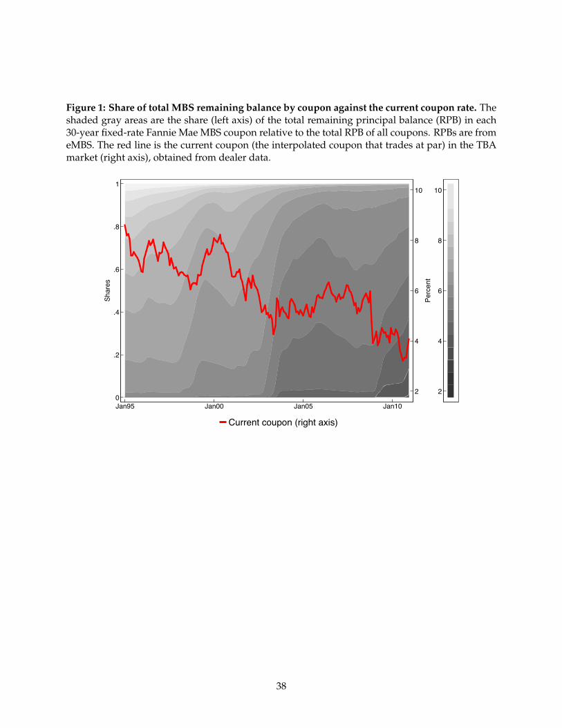
Figure 1: Share of total MBS remaining balance by coupon against the current coupon rate. Theshaded gray areas are the share (left axis) of the total remaining principal balance (RPB) in each30-year fixed-rate Fannie Mae MBS coupon relative to the total RPB of all coupons. RPBs are fromeMBS. The red line is the current coupon (the interpolated coupon that trades at par) in the TBAmarket (right axis), obtained from dealer data.

2

4

6

8

10

Perc

ent

0

.2

.4

.6

.8

1

Shar

es

Jan95 Jan00 Jan05 Jan10

2

4

6

8

10

Jan98Jul98Jan99Jul99Jan00

Current coupon (right axis)

38

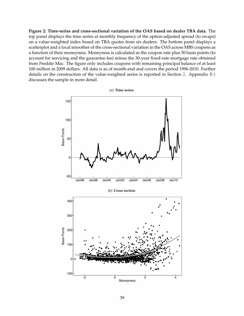
Figure 2: Time-series and cross-sectional variation of the OAS based on dealer TBA data. Thetop panel displays the time series at monthly frequency of the option-adjusted spread (to swaps)on a value-weighted index based on TBA quotes from six dealers. The bottom panel displays ascatterplot and a local smoother of the cross-sectional variation in the OAS across MBS coupons asa function of their moneyness. Moneyness is calculated as the coupon rate plus 50 basis points (toaccount for servicing and the guarantee fee) minus the 30-year fixed-rate mortgage rate obtainedfrom Freddie Mac. The figure only includes coupons with remaining principal balance of at least100 million in 2009 dollars. All data is as of month-end and covers the period 1996-2010. Furtherdetails on the construction of the value-weighted series is reported in Section 2. Appendix B.1discusses the sample in more detail.

(a) Time series

-50

0

50

100

150

Basi

s Po

ints

Jan96 Jan98 Jan00 Jan02 Jan04 Jan06 Jan08 Jan10

(b) Cross section

-100

0

100

200

300

400

Basi

s Po

ints

-2 0 2 4Moneyness

39

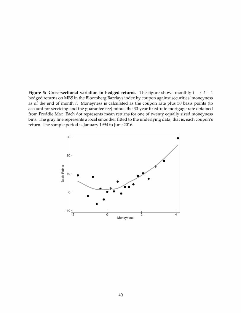
Figure 3: Cross-sectional variation in hedged returns. The figure shows monthly t → t + 1hedged returns on MBS in the Bloomberg Barclays index by coupon against securities’ moneynessas of the end of month t. Moneyness is calculated as the coupon rate plus 50 basis points (toaccount for servicing and the guarantee fee) minus the 30-year fixed-rate mortgage rate obtainedfrom Freddie Mac. Each dot represents mean returns for one of twenty equally sized moneynessbins. The gray line represents a local smoother fitted to the underlying data, that is, each coupon’sreturn. The sample period is January 1994 to June 2016.

-10

0

10

20

30

Basi

s Po

ints

-2 0 2 4Moneyness

40

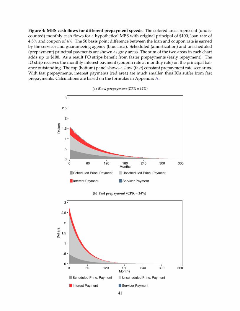
Figure 4: MBS cash flows for different prepayment speeds. The colored areas represent (undis-counted) monthly cash flows for a hypothetical MBS with original principal of $100, loan rate of4.5% and coupon of 4%. The 50 basis point difference between the loan and coupon rate is earnedby the servicer and guaranteeing agency (blue area). Scheduled (amortization) and unscheduled(prepayment) principal payments are shown as gray areas. The sum of the two areas in each chartadds up to $100. As a result PO strips benefit from faster prepayments (early repayment). TheIO strip receives the monthly interest payment (coupon rate at monthly rate) on the principal bal-ance outstanding. The top (bottom) panel shows a slow (fast) constant prepayment rate scenarios.With fast prepayments, interest payments (red area) are much smaller, thus IOs suffer from fastprepayments. Calculations are based on the formulas in Appendix A.

(a) Slow prepayment (CPR = 12%)

0

.5

1

1.5

2

2.5

3

Dol

lars

0 60 120 180 240 300 360Months

Scheduled Princ. Payment Unscheduled Princ. Payment

Interest Payment Servicer Payment

(b) Fast prepayment (CPR = 24%)

0

.5

1

1.5

2

2.5

3

Dol

lars

0 60 120 180 240 300 360Months

Scheduled Princ. Payment Unscheduled Princ. Payment

Interest Payment Servicer Payment

41

Figure 5: Visualization of the identification assumption for OASQ. The figure shows the OASon a IO, PO and pass-through for the same underlying collateral as a function of the prepaymentmultiple (Λ) on the physical prepayment speed. Higher Λ increases the market-implied prepay-ment speed relative to the physical one. The OAS on the IO (PO) declines (increases) in Λ. Thisfollows from the relation between the value of each strip and prepayments shown in Figure 4.The OAS on the pass-through in this example also declines in Λ because the pass-through is apremium security (PIO + PPO > $100). The three OAS differ at the physical speed (Λ = 1) but areequalized at the risk-neutral speed. This value of Λ defines the market implied prepayment speedand the OASQ.

OASOAS-Q

-100

-50

0

50

100

150

200

250

300

350

400

OAS

(bas

is po

ints

)

.9 1 1.1 1.2Λ

IO PO Pass-through

42

Figure 6: Survey-implied average prepayment rates at different levels of burnout. The figureshows the prepayment function in equation (4.2) with parameters b1, b2 and b3 set at their samplemeans. Differences in χ parametrize the burnout effect. Fast refinancers (group 1) and slow refi-nancers (group 2) are present in the pool with shares χ and 1− χ. As the share of more sensitiveborrowers χ falls, the pool’s overall sensitivity to interest rates is reduced. The vertical axis is the“conditional prepayment rate” (CPR, or annualized prepayment rate) and the horizontal axis is ameasure of the incentive to prepay the mortgage.

0

20

40

60

80

CPR

, in

perc

ent

-1 0 1 2 3 4 5INC (Average note rate - 10-year swap rate), in percent

χ = 1 χ=0.75 χ = 0.25 χ = 0

43

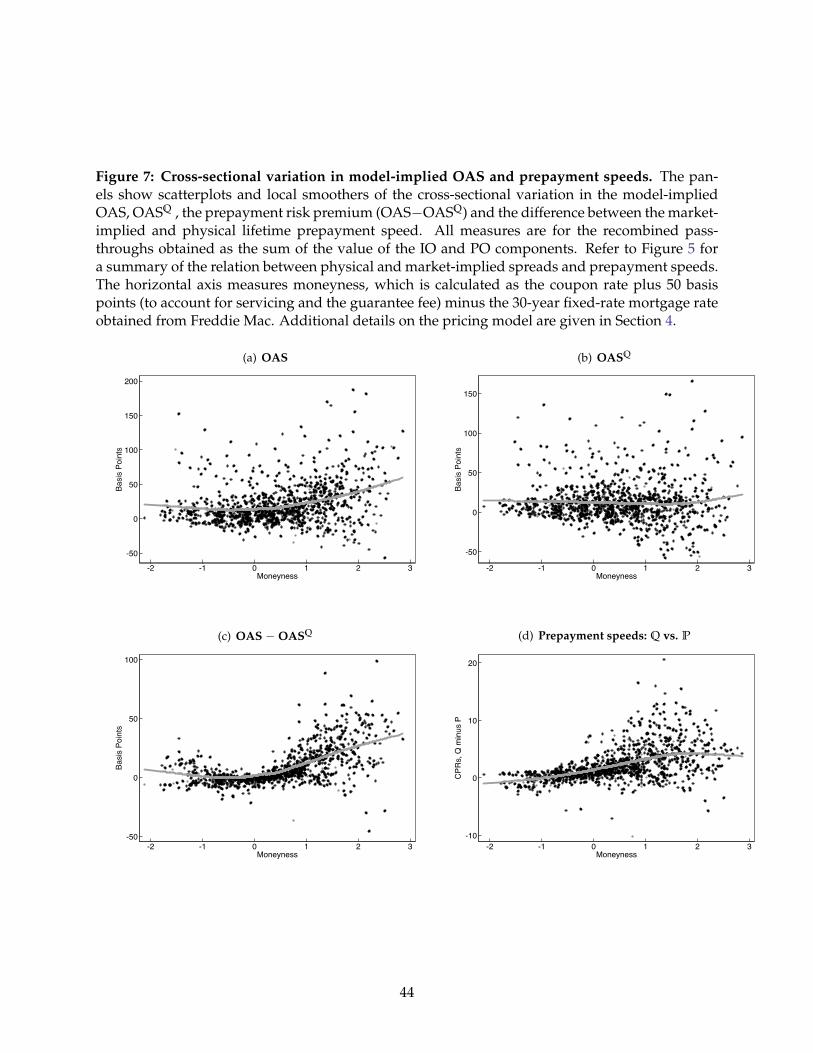
Figure 7: Cross-sectional variation in model-implied OAS and prepayment speeds. The pan-els show scatterplots and local smoothers of the cross-sectional variation in the model-impliedOAS, OASQ , the prepayment risk premium (OAS−OASQ) and the difference between the market-implied and physical lifetime prepayment speed. All measures are for the recombined pass-throughs obtained as the sum of the value of the IO and PO components. Refer to Figure 5 fora summary of the relation between physical and market-implied spreads and prepayment speeds.The horizontal axis measures moneyness, which is calculated as the coupon rate plus 50 basispoints (to account for servicing and the guarantee fee) minus the 30-year fixed-rate mortgage rateobtained from Freddie Mac. Additional details on the pricing model are given in Section 4.

(a) OAS

-50

0

50

100

150

200

Basi

s Po

ints

-2 -1 0 1 2 3Moneyness

(b) OASQ

-50

0

50

100

150

Basi

s Po

ints

-2 -1 0 1 2 3Moneyness

(c) OAS − OASQ

-50

0

50

100

Basi

s Po

ints

-2 -1 0 1 2 3Moneyness

(d) Prepayment speeds: Q vs. P

-10

0

10

20

CPR

s, Q

min

us P

-2 -1 0 1 2 3Moneyness

44

Figure 8: Time series of the OAS on the pass-through index from IO/PO strips. This figureshows time-series variation in OAS and OASQ on a value-weighted index computed from IO/POprices. To construct the index, we first average spreads across trusts for each coupon using marketweights. Then, for each month we average across coupons using each market value from TBAprices. For each trust, the value of the pass-through is the sum of the value of the IO and PO.Refer to Figure 5 for a summary of the relation between OAS and OASQ and to Section 4 for moredetails on the pricing model.

-50

0

50

100

150

Basis

Poi

nts

Jan96 Jan98 Jan00 Jan02 Jan04 Jan06 Jan08 Jan10

OAS OAS-Q

45

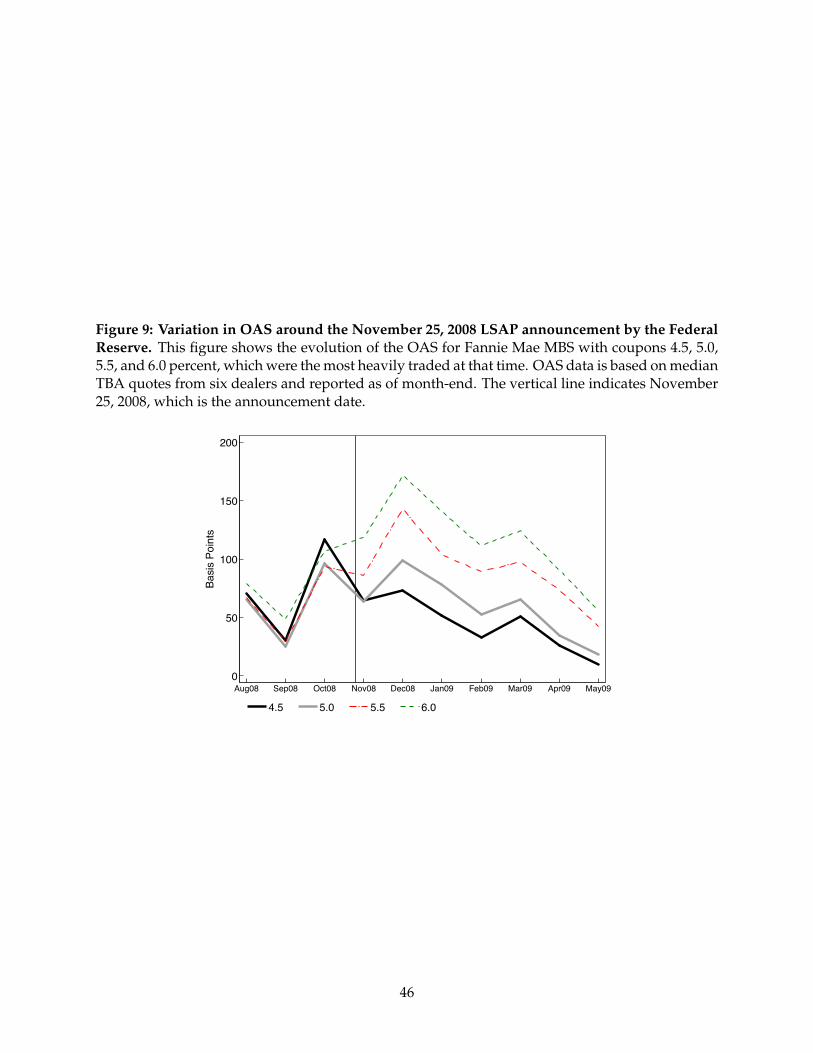
Figure 9: Variation in OAS around the November 25, 2008 LSAP announcement by the FederalReserve. This figure shows the evolution of the OAS for Fannie Mae MBS with coupons 4.5, 5.0,5.5, and 6.0 percent, which were the most heavily traded at that time. OAS data is based on medianTBA quotes from six dealers and reported as of month-end. The vertical line indicates November25, 2008, which is the announcement date.

0

50

100

150

200

Basis

Poi

nts

Aug08 Sep08 Oct08 Nov08 Dec08 Jan09 Feb09 Mar09 Apr09 May09

4.5 5.0 5.5 6.0

46

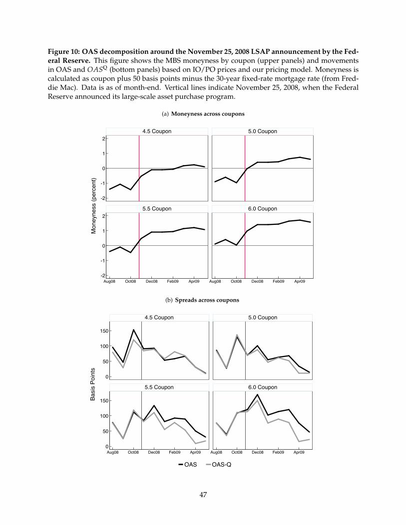
Figure 10: OAS decomposition around the November 25, 2008 LSAP announcement by the Fed-eral Reserve. This figure shows the MBS moneyness by coupon (upper panels) and movementsin OAS and OASQ (bottom panels) based on IO/PO prices and our pricing model. Moneyness iscalculated as coupon plus 50 basis points minus the 30-year fixed-rate mortgage rate (from Fred-die Mac). Data is as of month-end. Vertical lines indicate November 25, 2008, when the FederalReserve announced its large-scale asset purchase program.

(a) Moneyness across coupons

-2

-1

0

1

2

-2

-1

0

1

2

Aug08 Oct08 Dec08 Feb09 Apr09 Aug08 Oct08 Dec08 Feb09 Apr09

4.5 Coupon 5.0 Coupon

5.5 Coupon 6.0 Coupon

Mon

eyne

ss (p

erce

nt)

(b) Spreads across coupons

0

50

100

150

0

50

100

150

Aug08 Oct08 Dec08 Feb09 Apr09 Aug08 Oct08 Dec08 Feb09 Apr09

4.5 Coupon 5.0 Coupon

5.5 Coupon 6.0 Coupon

OAS OAS-Q

Basis

Poi

nts

47

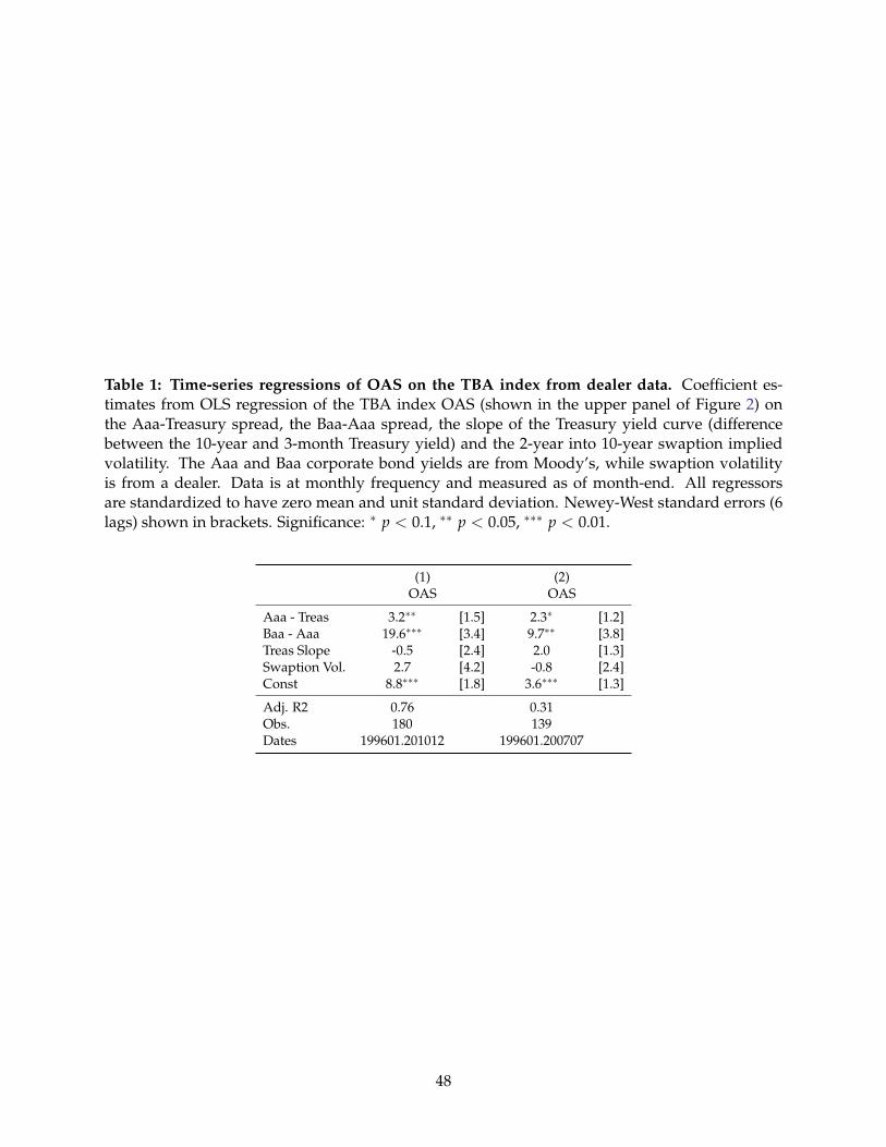
Table 1: Time-series regressions of OAS on the TBA index from dealer data. Coefficient es-timates from OLS regression of the TBA index OAS (shown in the upper panel of Figure 2) onthe Aaa-Treasury spread, the Baa-Aaa spread, the slope of the Treasury yield curve (differencebetween the 10-year and 3-month Treasury yield) and the 2-year into 10-year swaption impliedvolatility. The Aaa and Baa corporate bond yields are from Moody’s, while swaption volatilityis from a dealer. Data is at monthly frequency and measured as of month-end. All regressorsare standardized to have zero mean and unit standard deviation. Newey-West standard errors (6lags) shown in brackets. Significance: ∗ p < 0.1, ∗∗ p < 0.05, ∗∗∗ p < 0.01.

(1) (2)OAS OAS

Aaa - Treas 3.2∗∗ [1.5] 2.3∗ [1.2]Baa - Aaa 19.6∗∗∗ [3.4] 9.7∗∗ [3.8]Treas Slope -0.5 [2.4] 2.0 [1.3]Swaption Vol. 2.7 [4.2] -0.8 [2.4]Const 8.8∗∗∗ [1.8] 3.6∗∗∗ [1.3]

Adj. R2 0.76 0.31Obs. 180 139Dates 199601.201012 199601.200707

48

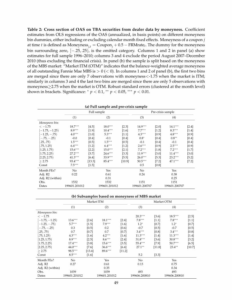
Table 2: Cross section of OAS on TBA securities from dealer data by moneyness. Coefficientestimates from OLS regressions of the OAS (annualized, in basis points) on different moneynessbin dummies, either including or excluding calendar month fixed effects. Moneyness of a coupon jat time t is defined as Moneynessj,t = Couponj + 0.5− FRMratet. The dummy for the moneynessbin surrounding zero, [−.25, .25), is the omitted category. Columns 1 and 2 in panel (a) showestimates for full sample 1996–2010; columns 3 and 4 exclude the period August 2007–December2010 (thus excluding the financial crisis). In panel (b) the sample is split based on the moneynessof the MBS market: “Market ITM (OTM)” indicates that the balance-weighted average moneynessof all outstanding Fannie Mae MBS is > 0 (< 0). In columns 1 and 2 of panel (b), the first two binsare merged since there are only 7 observations with moneyness<-1.75 when the market is ITM;similarly in columns 3 and 4 the last two bins are merged since there are only 5 observations withmoneyness≥2.75 when the market is OTM. Robust standard errors (clustered at the month level)shown in brackets. Significance: ∗ p < 0.1, ∗∗ p < 0.05, ∗∗∗ p < 0.01.

(a) Full sample and pre-crisis sampleFull sample Pre-crisis sample

(1) (2) (3) (4)

Moneyness bin:< −1.75 18.7∗∗∗ [4.5] 18.0∗∗∗ [2.3] 14.9∗∗∗ [2.0] 14.1∗∗∗ [2.4][−1.75,−1.25) 8.9∗∗∗ [1.9] 10.4∗∗∗ [1.6] 7.7∗∗∗ [1.2] 8.3∗∗∗ [1.4][−1.25,−.75) 4.0∗∗∗ [1.0] 5.3∗∗∗ [1.1] 4.3∗∗∗ [0.9] 4.8∗∗∗ [0.9][−.75,−.25) -0.0 [0.4] -0.1 [0.4] 0.8∗ [0.4] 0.8∗∗ [0.4][.25, .75) 1.5∗∗∗ [0.5] 1.5∗∗∗ [0.5] -0.1 [0.4] -0.1 [0.4][.75, 1.25) 6.4∗∗∗ [1.2] 6.4∗∗∗ [1.2] 2.6∗∗∗ [0.9] 2.5∗∗∗ [0.9][1.25, 1.75) 15.6∗∗∗ [2.2] 15.0∗∗∗ [2.1] 7.2∗∗∗ [1.8] 7.2∗∗∗ [1.7][1.75, 2.25) 27.2∗∗∗ [3.7] 24.6∗∗∗ [3.3] 11.9∗∗∗ [3.0] 11.4∗∗∗ [3.0][2.25, 2.75) 41.3∗∗∗ [6.4] 33.9∗∗∗ [5.5] 26.0∗∗∗ [5.3] 23.2∗∗∗ [5.2]≥ 2.75 93.4∗∗∗ [13.3] 85.4∗∗∗ [10.9] 50.5∗∗∗ [7.2] 47.1∗∗∗ [7.2]Const 7.5∗∗∗ [1.5] 0.5 [0.8]

Month FEs? No Yes No YesAdj. R2 0.22 0.61 0.24 0.38Adj. R2 (within) 0.31 0.25Obs. 1532 1532 1151 1151Dates 199601.201012 199601.201012 199601.200707 199601.200707

(b) Subsamples based on moneyness of MBS marketMarket ITM Market OTM

(1) (2) (3) (4)

Moneyness bin:< −1.75 20.3∗∗∗ [3.6] 18.5∗∗∗ [2.5][−1.75,−1.25) 13.6∗∗∗ [2.6] 18.1∗∗∗ [2.4] 7.8∗∗∗ [1.1] 7.8∗∗∗ [1.1][−1.25,−.75) 5.7∗∗∗ [1.5] 7.9∗∗∗ [1.6] 1.2∗ [0.7] 1.2∗ [0.7][−.75,−.25) 0.3 [0.5] 0.2 [0.6] -0.7 [0.5] -0.7 [0.5][.25, .75) 0.7 [0.7] 0.7 [0.7] 3.4∗∗∗ [0.8] 3.4∗∗∗ [0.8][.75, 1.25) 4.3∗∗∗ [1.6] 4.2∗∗∗ [1.6] 11.3∗∗∗ [1.4] 11.3∗∗∗ [1.4][1.25, 1.75) 8.9∗∗∗ [2.5] 8.6∗∗∗ [2.4] 31.8∗∗∗ [3.6] 30.8∗∗∗ [3.2][1.75, 2.25) 17.4∗∗∗ [3.8] 15.6∗∗∗ [3.5] 55.4∗∗∗ [7.9] 50.7∗∗∗ [6.5][2.25, 2.75) 44.0∗∗∗ [7.6] 36.6∗∗∗ [6.4] 27.1∗∗ [11.8] 23.4∗∗ [10.7]≥ 2.75 98.5∗∗∗ [13.4] 89.6∗∗∗ [11.2]Const 8.5∗∗∗ [1.6] 5.2 [3.3]

Month FEs? No Yes No YesAdj. R2 0.27 0.61 0.13 0.75Adj. R2 (within) 0.35 0.34Obs. 1039 1039 493 493Dates 199601.201012 199601.201012 199606.200810 199606.200810

49

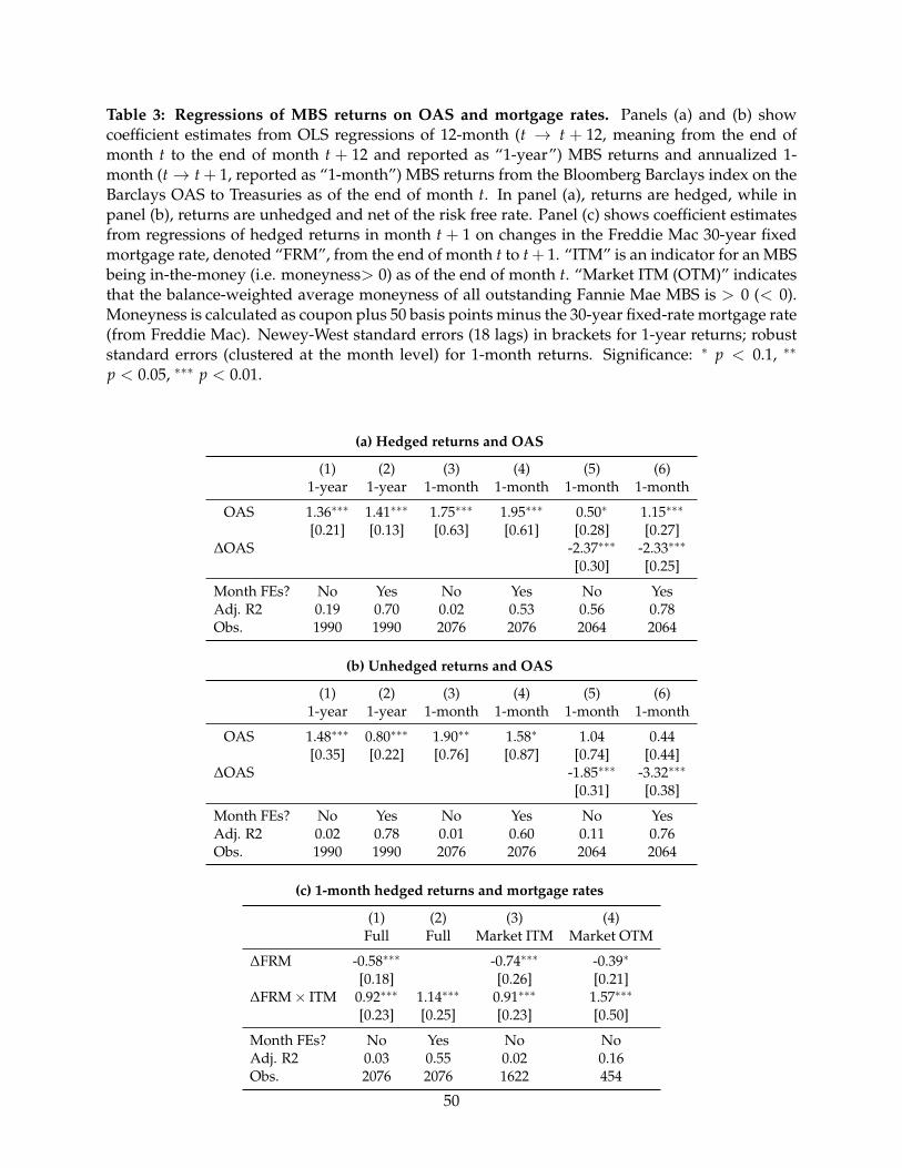
Table 3: Regressions of MBS returns on OAS and mortgage rates. Panels (a) and (b) showcoefficient estimates from OLS regressions of 12-month (t → t + 12, meaning from the end ofmonth t to the end of month t + 12 and reported as “1-year”) MBS returns and annualized 1-month (t→ t + 1, reported as “1-month”) MBS returns from the Bloomberg Barclays index on theBarclays OAS to Treasuries as of the end of month t. In panel (a), returns are hedged, while inpanel (b), returns are unhedged and net of the risk free rate. Panel (c) shows coefficient estimatesfrom regressions of hedged returns in month t + 1 on changes in the Freddie Mac 30-year fixedmortgage rate, denoted “FRM”, from the end of month t to t+ 1. “ITM” is an indicator for an MBSbeing in-the-money (i.e. moneyness> 0) as of the end of month t. “Market ITM (OTM)” indicatesthat the balance-weighted average moneyness of all outstanding Fannie Mae MBS is > 0 (< 0).Moneyness is calculated as coupon plus 50 basis points minus the 30-year fixed-rate mortgage rate(from Freddie Mac). Newey-West standard errors (18 lags) in brackets for 1-year returns; robuststandard errors (clustered at the month level) for 1-month returns. Significance: ∗ p < 0.1, ∗∗

p < 0.05, ∗∗∗ p < 0.01.

(a) Hedged returns and OAS

(1) (2) (3) (4) (5) (6)1-year 1-year 1-month 1-month 1-month 1-month

OAS 1.36∗∗∗ 1.41∗∗∗ 1.75∗∗∗ 1.95∗∗∗ 0.50∗ 1.15∗∗∗

[0.21] [0.13] [0.63] [0.61] [0.28] [0.27]∆OAS -2.37∗∗∗ -2.33∗∗∗

[0.30] [0.25]

Month FEs? No Yes No Yes No YesAdj. R2 0.19 0.70 0.02 0.53 0.56 0.78Obs. 1990 1990 2076 2076 2064 2064

(b) Unhedged returns and OAS

(1) (2) (3) (4) (5) (6)1-year 1-year 1-month 1-month 1-month 1-month

OAS 1.48∗∗∗ 0.80∗∗∗ 1.90∗∗ 1.58∗ 1.04 0.44[0.35] [0.22] [0.76] [0.87] [0.74] [0.44]

∆OAS -1.85∗∗∗ -3.32∗∗∗

[0.31] [0.38]

Month FEs? No Yes No Yes No YesAdj. R2 0.02 0.78 0.01 0.60 0.11 0.76Obs. 1990 1990 2076 2076 2064 2064

(c) 1-month hedged returns and mortgage rates

(1) (2) (3) (4)Full Full Market ITM Market OTM

∆FRM -0.58∗∗∗ -0.74∗∗∗ -0.39∗

[0.18] [0.26] [0.21]∆FRM× ITM 0.92∗∗∗ 1.14∗∗∗ 0.91∗∗∗ 1.57∗∗∗

[0.23] [0.25] [0.23] [0.50]

Month FEs? No Yes No NoAdj. R2 0.03 0.55 0.02 0.16Obs. 2076 2076 1622 454

50

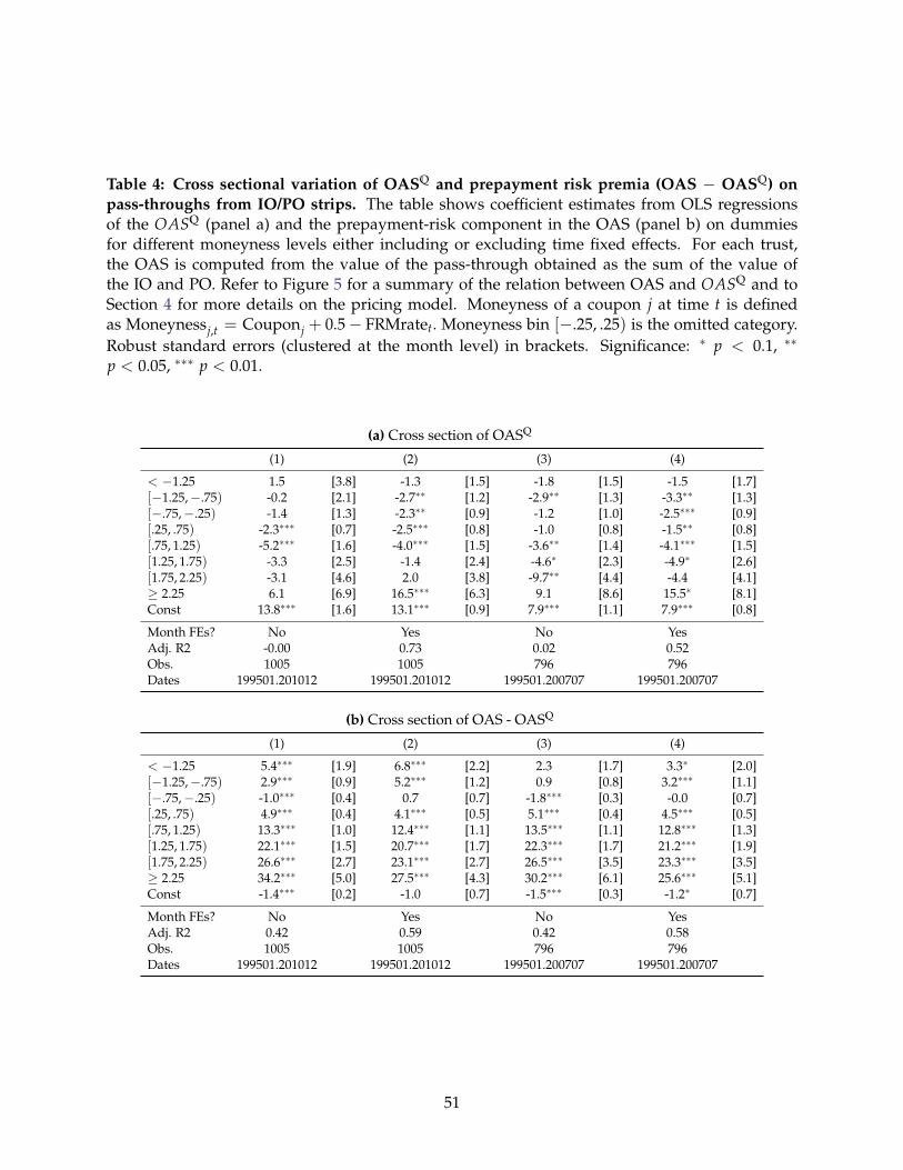
Table 4: Cross sectional variation of OASQ and prepayment risk premia (OAS − OASQ) onpass-throughs from IO/PO strips. The table shows coefficient estimates from OLS regressionsof the OASQ (panel a) and the prepayment-risk component in the OAS (panel b) on dummiesfor different moneyness levels either including or excluding time fixed effects. For each trust,the OAS is computed from the value of the pass-through obtained as the sum of the value ofthe IO and PO. Refer to Figure 5 for a summary of the relation between OAS and OASQ and toSection 4 for more details on the pricing model. Moneyness of a coupon j at time t is definedas Moneynessj,t = Couponj + 0.5− FRMratet. Moneyness bin [−.25, .25) is the omitted category.Robust standard errors (clustered at the month level) in brackets. Significance: ∗ p < 0.1, ∗∗

p < 0.05, ∗∗∗ p < 0.01.

(a) Cross section of OASQ

(1) (2) (3) (4)

< −1.25 1.5 [3.8] -1.3 [1.5] -1.8 [1.5] -1.5 [1.7][−1.25,−.75) -0.2 [2.1] -2.7∗∗ [1.2] -2.9∗∗ [1.3] -3.3∗∗ [1.3][−.75,−.25) -1.4 [1.3] -2.3∗∗ [0.9] -1.2 [1.0] -2.5∗∗∗ [0.9][.25, .75) -2.3∗∗∗ [0.7] -2.5∗∗∗ [0.8] -1.0 [0.8] -1.5∗∗ [0.8][.75, 1.25) -5.2∗∗∗ [1.6] -4.0∗∗∗ [1.5] -3.6∗∗ [1.4] -4.1∗∗∗ [1.5][1.25, 1.75) -3.3 [2.5] -1.4 [2.4] -4.6∗ [2.3] -4.9∗ [2.6][1.75, 2.25) -3.1 [4.6] 2.0 [3.8] -9.7∗∗ [4.4] -4.4 [4.1]≥ 2.25 6.1 [6.9] 16.5∗∗∗ [6.3] 9.1 [8.6] 15.5∗ [8.1]Const 13.8∗∗∗ [1.6] 13.1∗∗∗ [0.9] 7.9∗∗∗ [1.1] 7.9∗∗∗ [0.8]

Month FEs? No Yes No YesAdj. R2 -0.00 0.73 0.02 0.52Obs. 1005 1005 796 796Dates 199501.201012 199501.201012 199501.200707 199501.200707

(b) Cross section of OAS - OASQ

(1) (2) (3) (4)

< −1.25 5.4∗∗∗ [1.9] 6.8∗∗∗ [2.2] 2.3 [1.7] 3.3∗ [2.0][−1.25,−.75) 2.9∗∗∗ [0.9] 5.2∗∗∗ [1.2] 0.9 [0.8] 3.2∗∗∗ [1.1][−.75,−.25) -1.0∗∗∗ [0.4] 0.7 [0.7] -1.8∗∗∗ [0.3] -0.0 [0.7][.25, .75) 4.9∗∗∗ [0.4] 4.1∗∗∗ [0.5] 5.1∗∗∗ [0.4] 4.5∗∗∗ [0.5][.75, 1.25) 13.3∗∗∗ [1.0] 12.4∗∗∗ [1.1] 13.5∗∗∗ [1.1] 12.8∗∗∗ [1.3][1.25, 1.75) 22.1∗∗∗ [1.5] 20.7∗∗∗ [1.7] 22.3∗∗∗ [1.7] 21.2∗∗∗ [1.9][1.75, 2.25) 26.6∗∗∗ [2.7] 23.1∗∗∗ [2.7] 26.5∗∗∗ [3.5] 23.3∗∗∗ [3.5]≥ 2.25 34.2∗∗∗ [5.0] 27.5∗∗∗ [4.3] 30.2∗∗∗ [6.1] 25.6∗∗∗ [5.1]Const -1.4∗∗∗ [0.2] -1.0 [0.7] -1.5∗∗∗ [0.3] -1.2∗ [0.7]

Month FEs? No Yes No YesAdj. R2 0.42 0.59 0.42 0.58Obs. 1005 1005 796 796Dates 199501.201012 199501.201012 199501.200707 199501.200707

51

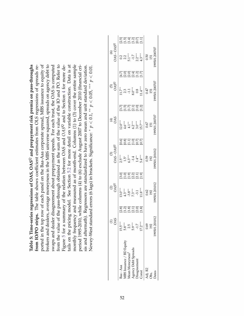
Tabl

e5:

Tim

e-se

ries

regr

essi

ons

ofO

AS,

OA

SQan

dpr

epay

men

tris

kpr

emia

onpa

ss-t

hrou

ghs

from

IO/P

Ost

rips

.Th

eta

ble

show

sco

effic

ient

esti

mat

esfr

omO

LSre

gres

sion

sof

spre

ads

re-

port

edin

the

top

row

ofea

chpa

nelo

nth

eBa

a-A

aaco

rpor

ate

spre

ad,M

BSis

suan

ceto

equi

tyof

brok

ers

and

deal

ers,

aver

age

mon

eyne

ssin

the

MBS

univ

erse

squa

red,

spre

ads

onag

ency

debt

tosw

aps

and

deal

erdi

sagr

eem

ent

abou

tpr

epay

men

tsp

eeds

.Fo

rea

chtr

ust,

the

OA

Sis

com

pute

dfr

omth

eva

lue

ofth

epa

ss-t

hrou

ghob

tain

edas

the

sum

ofth

eva

lue

ofth

eIO

and

PO.R

efer

toFi

gure

5fo

ra

sum

mar

yof

the

rela

tion

betw

een

OA

San

dO

ASQ

and

toSe

ctio

n4

for

mor

ede

-ta

ilson

the

pric

ing

mod

el.

See

Sect

ion

5.2

for

mor

ede

tail

onva

riab

leco

nstr

ucti

on.

Dat

ais

atm

onth

lyfr

eque

ncy

and

mea

sure

das

ofm

onth

-end

.C

olum

ns(1

)to

(3)

cove

rth

een

tire

sam

ple

peri

od19

95-2

010,

whi

leco

lum

ns(4

)to

(6)

excl

ude

Aug

ust

2007

toD

ecem

ber

2010

(fina

ncia

lcri

-si

san

daf

term

ath)

.R

egre

ssor

sar

est

anda

rdiz

edto

have

zero

mea

nan

dun

itst

anda

rdde

viat

ion.

New

ey-W

ests

tand

ard

erro

rs(6

lags

)in

brac

kets

.Sig

nific

ance

:∗p<

0.1,∗∗

p<

0.05

,∗∗∗

p<

0.01

.

(1)

(2)

(3)

(4)

(5)

(6)

OA

SO

ASQ

OA

S-O

ASQ

OA

SO

ASQ

OA

S-O

ASQ

Baa

-Aaa

15.5∗∗∗

[2.8

]13

.0∗∗∗

[3.0

]2.

5∗∗∗

[0.6

]12

.0∗∗∗

[3.7

]11

.7∗∗

[4.7

]0.

2[2

.5]

MBS

Issu

ance

/BD

Equi

ty5.

8∗∗∗

[1.2

]4.

3∗∗∗

[1.0

]1.

5∗[0

.8]

4.6∗∗∗

[1.5

]2.

3[2

.0]

2.2

[1.5

]M

ean

Mon

eyne

ss2

2.5

[1.8

]-3

.8∗∗

[1.9

]6.

3∗∗∗

[1.1

]4.

1∗∗

[1.7

]-1

.1[2

.0]

5.1∗∗∗

[1.4

]A

genc

yD

ebtS

prea

ds5.

9∗∗∗

[2.1

]7.

3∗∗∗

[2.2

]-1

.4[1

.0]

6.2∗∗∗

[2.1

]8.

0∗∗∗

[2.4

]-1

.7[1

.2]

Dis

agre

emen

t-1

.7[2

.0]

-3.1

[2.1

]1.

4∗∗

[0.7

]3.

0∗∗∗

[1.0

]0.

8[1

.2]

2.2∗∗∗

[0.7

]C

onst

17.2∗∗∗

[1.8

]11

.8∗∗∗

[1.9

]5.

4∗∗∗

[0.7

]15

.7∗∗∗

[1.2

]11

.4∗∗∗

[1.7

]4.

3∗∗∗

[1.1

]

Adj

.R2

0.69

0.62

0.59

0.67

0.47

0.50

Obs

.19

219

219

215

115

115

1D

ates

1995

01.2

0101

219

9501

.201

012

1995

01.2

0101

219

9501

.200

707

1995

01.2

0070

719

9501

.200

707

52

Appendix

A MBS cash flows

This Appendix provides detail on the calculation of cash flows for an MBS, which are used tocompute mortgage spreads as described in Section 2. Consider a fixed-rate MBS with an originalbalance of $1, and let θt be the “factor,” or remaining balance relative to origination, at date t.In level-payment fixed-rate mortgages, the principal is repaid gradually rather than with a bulletpayment at maturity and the borrower makes fixed payments every month. Denote the loan ma-turity measured in months by T (at the pool level, this is referred to as weighted average maturity,or WAM). Let k be the monthly installment from the borrower to the servicer, w the interest rate onthe loan (or weighted average coupon, WAC, at the pool level), and c the coupon paid to investors.The difference between the loan and coupon rates is earned by servicers or by the guaranteeingagency. To compute the fixed payment k note that, net of this payment, the loan balance absentany prepayment, denoted θt grows at rate (1 + w), or:

θt = (1 + w) θt−1 − k. (A.1)

Solving for θT = 0, it then follows that k =(

w(1+w)T

(1+w)T−1

). The evolution of the loan balance θt

allowing for early prepayment generalizes equation (A.1). After accounting for loan amortizationand unscheduled principal payments, the factor evolves according to:

θt = (1− SMMt−1)(1 + w)θt−1 − k θt, (A.2)

where w is the interest rate on the loan (or weighted average coupon, WAC) and k is the con-stant monthly payment composed of the scheduled principal and interest payments. SMMt is the“single month mortality,” or the fraction of the remaining balance that was prepaid in month tdue to unscheduled principal payments, and θt is the cumulated fraction of unit principal thathas not prepaid since the inception of the mortgage, which is also known as the survival factor,θt = ∏t−1

s=0(1− SMMs). It then follows that θt = θt × θt.1 Given prepayment rates, cash flowspassed through to investors per unit of principal are:

Xt = (θt−1 − θt) + c θt−1, (A.3)

where the principal payment is equal to the decline in principal (θt−1 − θt) and the coupon pay-ment from the borrower to the investor net of the servicing and agency guarantee fees is c θt−1.

1The prepayment speed is often reported in annualized terms, known as the “conditional prepayment rate” orCPRt = 1− (1− SMMt)

12.

1

B Data

B.1 TBA sample and data-quality filters

The sample used for the analysis in Sections 2.2 and 2.3 spans 1996 to 2010, reflecting limitedavailability of data on MBS in the TBA market prior to 1996, and a limited liquidity in IO/POstrips, which we use later in the paper to decompose the OAS, post 2010. The OAS we use are theaverage (within each coupon/month) across six dealers from which we collect data. We do notnecessarily have spreads for all dealers on the same coupons on each day. In addition, some of thedealers enter our data only after 1996. We clean each dealer’s data to prevent spreads from beinginfluenced by stale prices. To do so, we check whether a price for a coupon is unchanged relativeto the previous day. If it is, and if the 10-year Treasury yield changed by 3 basis points or moreon the same day (so we expect MBS prices to change), we drop the price and the correspondingspread. If the price is not constant, but had been constant more than twice in the same calendarmonth on days when the Treasury yield moves, we similarly drop it.

Descriptive statistics of the monthly coupon-level sample used for the analysis in Sections 2.2and 2.3 are provided in Table A-1. The coupons in the sample change over time (as illustrated inFigure 1 in the main text), so that the data form an unbalanced panel.

Table A-1: Descriptive statistics of TBA sample. Based on Fannie Mae pass-through couponsfrom 1996-2010 for which we have OAS quotes from at least one dealer, subject to the data qualityfilters described in Section B.1. Data frequency is monthly; spreads and moneyness (= couponplus 0.5 minus current FRM rate) are as of month-end. RPB stands for the total remaining principalbalance in a coupon. Factor means current face value divided by issuance amount. Data on RPBs,factors, and weighted average loan ages are from eMBS.

Mean Std. Dev. p5 p25 p50 p75 p95 Obs.OAS (basis points, annual) 23.12 50.66 -16.45 -2.27 9.05 28.03 120.00 1532Coupon (percent) 6.53 1.49 4.00 5.50 6.50 7.50 9.00 1532Moneyness (percent) 0.56 1.40 -1.64 -0.58 0.51 1.60 2.93 1532RPB (2009 USD, million) 126928.83 151009.18 590.43 9091.44 66862.53 194624.09 443893.38 1532Factor of most recent vintage 0.89 0.21 0.26 0.91 0.98 0.99 1.00 1530Weighted average loan age (months) 47.44 33.51 8.67 25.37 38.36 58.93 128.27 1532

B.2 Stripped MBS data-quality filters

We start with daily price quotes from a large dealer for the period 1995 to 2010, and then cleanthese data using the following steps:

1. Remove/correct obvious outliers (such as prices of 0 or a few instances where IO and POprices were inverted).

2. Remove prices that are stale (defined as a price that does not change from previous daydespite a change in the 10-year yield of more than 3 basis points). In case of smaller yield

2

changes, we check the previous 10 days and remove a price if there were more than twoinstances of stale prices on that security over that period.

3. For a subsample of trusts and months (starting in June 1999), we also have price quotes fromtwo additional dealers. When available, we compare these prices (their average if both areavailable) to the price quoted by our dealer. When they are more than 5% apart, or if theoverall range of price quotes is larger than 0.1 times the average price, we do not use ourprice quote in the analysis. This applies to about 10% of our price quotes.

4. Only retain trusts for which we have both the IO and PO strips, and which we can link todata on the underlying pool of mortgages (from eMBS). This restriction eliminates IO stripsbacked by excess servicing rights, for instance.

5. Only retain trusts for which the price on the recombined pass-through (= PPO + PIO) iswithin $2 of the TBA price of the corresponding coupon. (We also drop trusts if on that daywe do not have a clean TBA price for the corresponding coupon.)

6. Only retain trusts with a factor (= current face value divided by issuance amount) of morethan 5%.

7. Only retain trusts that we can match to a Bloomberg prepayment survey with the samecoupon and absolute differences in WAC and WAM smaller than 0.3 percentage points and60 months, respectively. (This affects almost exclusively observations before 2003, as we donot have individual vintages in the survey in the early years.)

Following these steps, the sample includes 3713 trust-month observations, or about 19 per month.The year with the lowest number of observations is 1999, where we have an average of 10 trustsper month, while after 2005 we have at least 20 trusts in all but one month.

C OAS smile: Robustness

This Appendix provides additional evidence on the smile-shaped pattern of the OAS in the crosssection of TBA coupons, which is a key empirical result as discussed in Section 2.3. We showrobustness to dropping periods of financial stress, stability across sub-periods, and regressionestimates when excluding outlier observations, MBS coupons with relatively low balances, orcoupons that may be “burned out” (as indicated by a low remaining factor).

One potential concern about the OAS pattern shown in panel (b) of Figure 2 is that it maybe unduly influenced by periods of financial stress. Panel (a) of Figure A-1 replicates Figure 2when excluding the post-July 2007 period, and the period from September 1998 to January 1999,when liquidity in many U.S. fixed income markets dried up following the failure of Long-TermCapital Management (LTCM). The figure shows that the distinctive smile pattern remains presenteven without these periods. Panel (b) of Figure A-1 provides evidence on sub-sample stability by

3

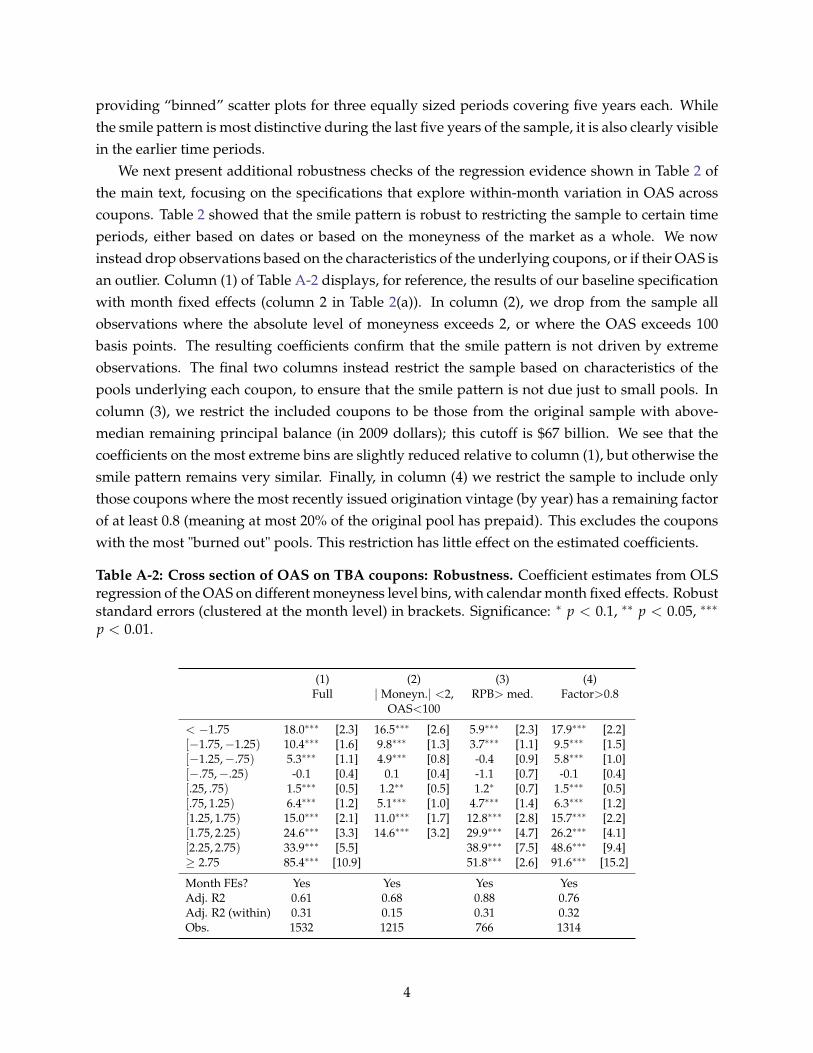
providing “binned” scatter plots for three equally sized periods covering five years each. Whilethe smile pattern is most distinctive during the last five years of the sample, it is also clearly visiblein the earlier time periods.

We next present additional robustness checks of the regression evidence shown in Table 2 ofthe main text, focusing on the specifications that explore within-month variation in OAS acrosscoupons. Table 2 showed that the smile pattern is robust to restricting the sample to certain timeperiods, either based on dates or based on the moneyness of the market as a whole. We nowinstead drop observations based on the characteristics of the underlying coupons, or if their OAS isan outlier. Column (1) of Table A-2 displays, for reference, the results of our baseline specificationwith month fixed effects (column 2 in Table 2(a)). In column (2), we drop from the sample allobservations where the absolute level of moneyness exceeds 2, or where the OAS exceeds 100basis points. The resulting coefficients confirm that the smile pattern is not driven by extremeobservations. The final two columns instead restrict the sample based on characteristics of thepools underlying each coupon, to ensure that the smile pattern is not due just to small pools. Incolumn (3), we restrict the included coupons to be those from the original sample with above-median remaining principal balance (in 2009 dollars); this cutoff is $67 billion. We see that thecoefficients on the most extreme bins are slightly reduced relative to column (1), but otherwise thesmile pattern remains very similar. Finally, in column (4) we restrict the sample to include onlythose coupons where the most recently issued origination vintage (by year) has a remaining factorof at least 0.8 (meaning at most 20% of the original pool has prepaid). This excludes the couponswith the most "burned out" pools. This restriction has little effect on the estimated coefficients.

Table A-2: Cross section of OAS on TBA coupons: Robustness. Coefficient estimates from OLSregression of the OAS on different moneyness level bins, with calendar month fixed effects. Robuststandard errors (clustered at the month level) in brackets. Significance: ∗ p < 0.1, ∗∗ p < 0.05, ∗∗∗

p < 0.01.

(1) (2) (3) (4)Full |Moneyn.| <2, RPB> med. Factor>0.8

OAS<100

< −1.75 18.0∗∗∗ [2.3] 16.5∗∗∗ [2.6] 5.9∗∗∗ [2.3] 17.9∗∗∗ [2.2][−1.75,−1.25) 10.4∗∗∗ [1.6] 9.8∗∗∗ [1.3] 3.7∗∗∗ [1.1] 9.5∗∗∗ [1.5][−1.25,−.75) 5.3∗∗∗ [1.1] 4.9∗∗∗ [0.8] -0.4 [0.9] 5.8∗∗∗ [1.0][−.75,−.25) -0.1 [0.4] 0.1 [0.4] -1.1 [0.7] -0.1 [0.4][.25, .75) 1.5∗∗∗ [0.5] 1.2∗∗ [0.5] 1.2∗ [0.7] 1.5∗∗∗ [0.5][.75, 1.25) 6.4∗∗∗ [1.2] 5.1∗∗∗ [1.0] 4.7∗∗∗ [1.4] 6.3∗∗∗ [1.2][1.25, 1.75) 15.0∗∗∗ [2.1] 11.0∗∗∗ [1.7] 12.8∗∗∗ [2.8] 15.7∗∗∗ [2.2][1.75, 2.25) 24.6∗∗∗ [3.3] 14.6∗∗∗ [3.2] 29.9∗∗∗ [4.7] 26.2∗∗∗ [4.1][2.25, 2.75) 33.9∗∗∗ [5.5] 38.9∗∗∗ [7.5] 48.6∗∗∗ [9.4]≥ 2.75 85.4∗∗∗ [10.9] 51.8∗∗∗ [2.6] 91.6∗∗∗ [15.2]

Month FEs? Yes Yes Yes YesAdj. R2 0.61 0.68 0.88 0.76Adj. R2 (within) 0.31 0.15 0.31 0.32Obs. 1532 1215 766 1314

4

Figure A-1: OAS smile: robustness and subsamples. Panel (a) displays a scatterplot and a lo-cal smoother of the cross-sectional variation in OAS for MBS coupons with remaining principalbalance (in 2009 dollars) of $100 million or more, excluding from the sample the months Septem-ber 1998 to January 1999 (LTCM turmoil) and August 2007 to December 2010 (financial crisis andaftermath). Panel (b) displays “binned” scatterplots for three five-year subsamples, where eachdot represents mean OAS for one of ten equal-sized moneyness bins. The lines represent a lo-cal smoother fitted to the underlying data (i.e., each coupon’s OAS, not just the moneyness binaverages).

(a) Excluding periods of financial stress

-100

-50

0

50

100

150

Basi

s Po

ints

-2 0 2 4Moneyness

(b) Five-year subsamples

0

50

100

150

200

Basi

s Po

ints

-2 0 2 4Moneyness

1996-2000 2001-2005 2006-2010

5

D Expected return derivations

In this Appendix, we derive the relation between OAS and future excess returns (2.3) and therelation between contemporaneous excess returns and changes in OAS shown in (2.4). We finallyshow that the expected hedged return under the interest-rate-risk-neutral measure Qr equals theexpected hedged return under the physical measure P.

Derivation of (2.3). We begin by showing that the OAS can be approximated as a weightedaverage of future excess returns. Approximating the right hand side of (2.2) around 0 excessreturn, we obtain

∂ ∏kj=1

(1 + rt+j + E

Qrt+j−1

[rxt+j

])−1

∂EQrt+j−1

[rxt+j

]∣∣∣∣∣∣∣E

Qrt+j−1[rxt+j]=0

= − 11 + rt+j

k

∏j=1

1(1 + rt+j

) ,

so that (2.2) becomes

Pt ≈ EQrt

[T−t

∑k=1

Xk

∏kj=1(1 + rt+j

) (1−k

∑l=1

EQrt+l−1 [rxt+l ]

1 + rt+l

)].

Similarly, approximating the right hand side of (2.1) around 0 OAS, we can express

∂ ∏kj=1(1 + rt+j + OASt

)−1

∂OASt

∣∣∣∣∣∣OASt=0

= −k

∑l=1

11 + rt+l

k

∏j=1

1(1 + rt+j

) ,

so that (2.1) becomes

Pt ≈ EQrt

[T−t

∑k=1

Xk

∏kj=1(1 + rt+j

) (1−k

∑l=1

OASt

1 + rt+l

)].

Comparing these two expressions, we obtain

OAStEQrt

[T−t

∑k=1

Xk

∏kj=1(1 + rt+j

) k

∑l=1

11 + rt+l

]= E

Qrt

[T−t

∑k=1

Xk

∏kj=1(1 + rt+j

) k

∑l=1

EQrt+l−1 [rxt+l ]

1 + rt+l

],

and rearranging we obtain (2.3), where weights are:

wkt =T−t

∑l=k

Xt+l

∏lj=1(1+rt+l)

11+rt+k

EQrt

[∑T−t

k=11

1+rt+k∑T−t

l=kXt+l

∏lj=1(1+rt+j)

] .

6

Derivation of (2.4). To understand the link between realized excess returns and changes in theOAS, from (2.1), the OAS at date t + 1 is

Pt+1 = EQrt+1

[T−t−1

∑k=1

Xt+1+k

∏kj=1(1 + rt+1+j + OASt+1

)] .

Applying a first order Taylor approximation around the OAS remaining the same between datest and t + 1, the price next period can be approximated by

Pt+1 ≈ EQrt+1

[T−t−1

∑k=1

Xt+1+k

∏kj=1(1 + rt+1+j + OASt

)]+ ∂Pt+1

∂OAS∆OASt+1,

where ∆OASt+1 = OASt+1 − OASt is the change in the OAS. Thus, the one period return toholding the MBS can be expressed as

1 + rt+1 + rxt+1 =Pt+1 + Xt+1

Pt

≈E

Qrt+1

[∑T−t−1

k=1Xt+1+k

∏kj=1(1+rt+1+j+OASt)

]+ Xt+1 +

∂Pt+1∂OAS ∆OASt+1

Pt

= (1 + rt+1 + OASt)

EQrt+1

[∑T−t

k=1Xt+k

∏kj=1(1+rt+j+OASt)

]E

Qrt

[∑T−t

k=1Xt+k

∏kj=1(1+rt+j+OASt)

] +1Pt

∂Pt+1

∂OAS∆OASt+1,

where the last equality uses the fact that 1 + rt+1 + OASt and Xt+1 are known at date t + 1, sothat we can bring Xt+1 inside the date t + 1 expectations operator and factor 1 + rt+1 + OASt

from the date t + 1 expectation. Since the ratio of expectations is approximately 1, we obtain(2.4), where duration Dt is defined as − 1

Pt

∂Pt+1∂OAS . As discussed in the main text, this expression is

the analog to what Shiller et al. (1983) derive in the context of coupon-bearing Treasuries. Thisapproximate relation between returns and changes in OAS is also employed by practitioners (seeLehman Brothers, 2008, for example).

Expected excess returns under P and Qr. Using the fund separation theorem (see e.g. Merton,1972), we can represent the return on the MBS as

rxt+1 =Nr

∑j=1

Ct

(rxt+1, zj

t+1

)Vt

(zj

t+1

) zjt+1 +

Np

∑j=1

Ct

(rxt+1, pj

t+1

)Vt

(pj

t+1

) pjt+1 + εt+1 (D.1)

≡Nr

∑j=1

βirj,tz

jt+1 +

Np

∑j=1

βipj,t pj

t+1 + εt+1,

7

where

zjt+1

Nr

j=1are the one period excess returns on a set of portfolios that spans interest rate

uncertainty, and

pjt+1

Np

j=1are the one-period excess returns on a set of portfolios that spans

the prepayment risk that is orthogonal to interest rates. Here, Vt and Ct represent conditionalvariance and covariance, respectively. Thus, (D.1) represents excess returns on the MBS in terms ofits beta with respect to interest rate uncertainty spanning portfolios, non-interest rate prepaymentuncertainty spanning portfolios and idiosyncratic risk, εt+1.

The return on the hedged portfolio is then given by

rxt+1 −Nr

∑j=1

βirj,tz

jt+1 =

Np

∑j=1

βipj,t pj

t+1 + εt+1.

Then the expected hedged return under the interest-rate-neutral measure Qr is given by

EQrt

[rxt+1 −

Nr

∑j=1

βirj,tz

jt+1

]= E

Qrt

[Np

∑j=1

βipj,t pj

t+1 + εt+1

]= Et

[Mrt

(Np

∑j=1

βipj,t pj

t+1 + εt+1

)],

whereMr,t+1 is the change of measure between P and Qr. Since

zjt+1

Nr

j=1span the interest rate

uncertainty,Mr,t+1 can be represented as a portfolio of

zjt+1

Nr

j=1

Mr,t+1 = m0t +Nr

∑j=1

mjtzjt+1,

with 1 = m0t + ∑Nrj=1 mjtEt

[zj

t+1

]. Thus

EQrt

[rxt+1 −

Nr

∑j=1

βirj,tz

jt+1

]= Et

[(m0t +

Nr

∑j=1

mjtzjt+1

)(Np

∑j=1

βipj,t pj

t+1 + εt+1

)]

= Et

[m0t +

Nr

∑j=1

mjtzjt+1

]Et

[Np

∑j=1

βipj,t pj

t+1 + εt+1

]

= Et

[Np

∑j=1

βipj,t pj

t+1 + εt+1

],

where the second equality uses the fact that zjt+1 and pj

t+1 are uncorrelated and the third equalityuses the fact that the change of measureMr,t+1 is a martingale.

8

E Additional details on model

In this Appendix, we describe more formally, and under more general assumptions on the evo-lution of the term structure of interest rates, the simple framework presented in Section 3 in themain text. We show that the simple intuitions for the sources of risk premia reflected in the OAScarry through even under these more general assumptions.

We consider a complete probability space (Ω,F , P), where Ω is the set of states of nature withgeneric element ω, F is the σ-algebra of observable events and P is a probability measure on(Ω, P). We assume that the uncertainty in the economy is generated by a N-dimensional Brow-nian motion Zt and a Poisson process Jt, with Jt denoting the number of jumps up to time t. Wefurther partition the Brownian motion Zt into Nr shocks that affect the risk-free interest rate in

the economy and N − Nr shocks that do not: Zt =[

Z′rt Z′γt

]′. The Poisson process Jt captures

liquidity shocks to the MBS market and arrives with intensity µt; if a jump occurs at date t, thesecurities written on pool j lose a fraction αjt of their market value.

Consider a mortgage pool j with coupon rate cj, remaining principal balance θjt at time t andmaturity date Tj. As in Appendix A, let θjt be the remaining loan balance absent unscheduledprepayment at date t and cj is the fixed interest rate paid by the mortgagor (usually cj = cj +

50bps). Analogously to (A.1), in continuous time, this loan balance evolves as

∂θjt

∂t= cj θjt − k,

where k is, as before, the fixed payment from the borrower to the servicer. Solving for θjT = 0 andθjt = θj0, we obtain that the loan balance evolves as

θjt = θj0ecjTj − ecjt

ecjTj − 1,

where θj0 is the balance at origination and the fixed payment k is(

cj

ecjT−1

). Denote by S∗jt the

cumulative unscheduled prepayments, so that the remaining principal balance at date t is

θjt = e−S∗jt θjt.

We assume that the cumulative unscheduled prepayments can be represented as

S∗jt =∫ t

0s∗judu,

where s∗jt is a function of the interest rate incentive cj − ρt, where ρt is the interest rate on newloans, and a vector of parameters γt = (γ1t, γ2t, . . . , γΓt):

s∗jt = f(γt, cj − ρt

).

9

Finally, let Sjt be the full (that is, the sum of both scheduled and unscheduled) cumulative prepay-ments, so that

θjt = e−Sjt θj0,

where θj0 ≡ θj0. With this notation, the cash-flows received by investors in an IO strip on pool j aredXjt,IO = cjθjtdt, by investors in a PO strip on pool j are dXjt,PO = −dθjt, and by investors in thepass-through on pool j (the combination, denoted “PT,” of IO and PO) are dXjt,PT = cjθjtdt− dθjt.

Under the assumption of no arbitrage, there exists a stochastic discount factor that prices allthe assets in the economy, given by

dMt

Mt= exp

(−rtdt− π′rtdZrt − π′γtdZγt − πltdJt

),

where rt is the equilibrium risk-free rate, πrt is the vector of the prices of risk associated withinnovations affecting the term structure of interest rates in the economy (including ρt), πγt is thevector of the prices of risk associated with the innovations to the non-interest rate factors, andπlt is the price of risk associated with the liquidity shocks dJt. Associated with the stochasticdiscount factor is the risk-neutral measure Q. In addition to the risk-neutral measure, we considertwo intermediate changes of measure: one that is risk-neutral with respect to the interest rateshocks only, Qr, and one that is risk-neutral with respect to all Brownian shocks, Qr,γ. Thesetwo measures are defined, respectively, by their Radon-Nikodym derivatives with respect to thephysical measure P:

dQr

dP= exp

(−1

2|πrt|2 dt− π′rtdZrt

)dQr,γ

dP= exp

(−1

2

(|πrt|2 + |πγt|2

)dt− π′rtdZrt − π′γtdZγt

).

We can now introduce our two measures of the option-adjusted spread. Let Pk,jt be the marketprice of a security of type k ∈ IO, PO, PT on pool j at time t. The market price is given by

Pk,jt = Et

[∫ +∞

0

Mt+s

MtdXk,jt+s

]= E

Qt

[∫ +∞

0exp

(−∫ s

0rt+udu

)dXk,jt+s

],

where the second equality uses the definition of the risk-neutral measure Q. The traditional OASis defined implicitly through

Pk,jt = EQrt

[∫ +∞

0exp

(−∫ s

0rt+udu−OASk,jts

)dXk,jt+s

], (E.1)

10

while the prepayment-risk-neutral OAS, or OASQ, is defined implicitly through

Pk,jt = EQr,γt

[∫ +∞

0exp

(−∫ s

0rt+udu−OASQ

k,jts)

dXk,jt+s

]. (E.2)

As we show in Appendix D, the OAS is a weighted average of expected excess returns on thesecurity. We follow the same logic here and replace the average OAS over the security’s lifetimewith a stream of instantaneous OAS, so that (E.1) and (E.2) become

Pk,jt = EQrt

[∫ +∞

0exp

(−∫ s

0

[rt+u + OASk,jt+u

]du)

dXk,jt+s

]Pk,jt = E

Qr,γt

[∫ +∞

0exp

(−∫ s

0

[rt+u + OASQ

k,jt+u

]du)

dXk,jt+s

].

Differentiating both sides, we obtain

−EQrt[dPk,jt

]= −

(rt + OASk,jt

)Pk,jt−dt + E

Qrt[dXk,jt

]−E

Qr,γt[dPk,jt

]= −

(rt + OASQ

k,jt

)Pk,jt−dt + E

Qr,γt[dXk,jt

]−E

Qt[dPk,jt

]= −rtPk,jt−dt + E

Qt[dXk,jt

].

Comparing the three expressions for the equilibrium price, we can represent OASk,jt and OASQk,jt

as

OASk,jtPk,jt−dt = EQrt[dPk,jt + dXk,jt

]−E

Qt[dPk,jt + dXk,jt

]OASQ

k,jtPk,jt−dt = EQr,γt[dPk,jt + dXk,jt

]−E

Qt[dPk,jt + dXk,jt

].

Applying Ito’s lemma, we obtain

dPk,jt =∂Pk,jt

∂tdt +

∂Pk,jt

∂ρtdρt +

∂Pk,jt

∂γ′tdγt +

12

∂2Pk,jt

∂ρ2t〈dρt〉2 +

12

tr

(〈dγt〉2

∂2Pk,jt

∂γ∂γ′

)

+∂Pk,jt

∂ρt∂γ′t〈dρt, dγt〉+

[Pk,jt − Pk,jt−

]dθjt = −cj

ecjt

ecjTj − 1e−S∗jt θj0dt− θjts∗jtdt.

Since the evolution of the remaining principal balance is locally deterministic, the cash-flows ofeach security – the IO strip, the PO strip and the pass-through – written on pool j are locallydeterministic as well. Thus, the expected cash-flows E

(·)t[dCk,jt

]are independent of the measure

used to take the expectation. Similarly, the quadratic variation terms, 〈·〉, in the evolution of theprice are invariant with respect to the change of measure. If the local uncertainty in ρt and γt

is driven by Brownian innovations, the quadratic variation terms above can be expressed as thecorresponding variance-covariance matrices. Notice, finally, that the measures P, Qr and Qr,γ all

11

take the physical evolution of the jump process, so that the expectation of the jump componentof the price are equivalent under the three measures. Thus, the expressions for the OASk,jt andOASQ

k,jt become

OASk,jtPk,jt−dt =(

EQrt −E

Qt

) [∂Pk,jt

∂γ′tdγt

]+(

EQt −EP

t

)[dJt] αjPk,jt− (E.3)

OASQk,jtPk,jt−dt =

(E

Qt −EP

t

)[dJt] αjPk,jt− . (E.4)

Thus, the traditional OAS combines the prepayment risk premium

1Pk,jt−

1dt

(E

Qrt −E

Qt

) [∂Pk,jt

∂γ′tdγt

],

with the liquidity risk premium1dt

(E

Qt −EP

t

)[dJt] αj.

The prepayment-risk-neutral OAS, on the other hand, is only composed of the liquidity risk pre-mium. Under the assumption that all securities written on pool j lose the same fraction αjt of theirvalue when a liquidity jump occurs, OASQ is equal for all securities written on the pool, since theliquidity risk premium depends only on the difference between the risk-neutral and the physicalprobabilities of the jump occurring, 1

dt

(E

Qt −EP

t

)[dJt], and the loss in valuation due to the jump

OASQIO,jt = OASQ

PO,jt = OASQPT,jt =

1dt

(E

Qt −EP

t

)[dJt] αjt. (E.5)

Thus, Proposition 4.1 holds.Consider now the example in Section 3. In Section 3, we assume that the risk-free rate and

mortgage rate are constant and equal to each other, so that rt = ρt = r, that, under the physicalmeasure P, the non-interest-rate factors γt affecting prepayment follow a Brownian motion withdrift µγ and volatility σγ

dγt = µγdt + σγdZγt,

and that the arrival rate of the Poisson liquidity jump is µt. Thus,

(E

Qrt −E

Qt

) [∂Pk,jt

∂γ′tdγt

]=

∂Pk,jt

∂γ′tσγπγ,

1dt

(E

Qt −EP

t

)[dJt] = µt (πlt − 1) .

Substituting into (E.3) – (E.4), we obtain that the OAS is given by (3.2) and the OASQ by (3.5).

12

F Pricing model details

F.1 Interest rate model

We assume that swap rates follow a three-factor Heath, Jarrow, and Morton (1992) (HJM) model.Let f (t, T) denote the time t instantaneous forward interest rate for risk-free borrowing and lend-ing at time T. We model the forward rate dynamics under the (interest rate) risk-neutral measureas

d f (t, T) = µ f (t, T) dt +3

∑i=1

σf ,i (t, T) dWQi,t ,

where WQit are independent standard Weiner processes under the risk-neutral measure Q, and,

under no arbitrage, the expected change in the forward rate is given by

µ f (t, T) =3

∑i=1

σf ,i (t, T)∫ T

tσf ,i (t, u) du.

Thus, the risk-neutral dynamics of the instantaneous forward rate are completely determined bythe initial forward rate curve and the forward rate volatility functions, σf ,i (t, T). Similarly to Trolleand Schwartz (2009), we assume that the volatility function of each factor σf ,i (t, T) is

σf ,i (t, T) = (α0,i + α1,i (T − t)) e−γi(T−t). (F.1)

This specification has the advantage of allowing for a wide range of shocks to the forward ratecurve while ensuring that the forward rate model above is Markovian.

Trolle and Schwartz (2009) show that, setting the volatility of the forward rates to be as in (F.1),the time t price of a zero-coupon bond maturing at time T, P (t, T), is given by

P (t, T) ≡ exp−∫ T

tf (t, u) du

=

P (0, T)P (0, t)

exp

3

∑i=1

Bxi (T − t) xit +3

∑i=1

6

∑j=1

Bφji (T − t) φji,t

,

where the state variables

xit, φji,t

follow

dxit = −γixitdt + dWQit

dφ1i,t = (xit − γiφ1i,t) dt

dφ2i,t = (1− γiφ2i,t) dt

dφ3i,t = (1− 2γiφ3i,t) dt

dφ4i,t = (φ2i,t − γiφ4i,t) dt

dφ5i,t = (φ3i,t − 2γiφ5i,t) dt

dφ6i,t = (2φ5i,t − 2γiφ6i,t) dt.

13

The coefficients

Bxi , Bφji

are functions of the parameters of the volatility function and the time

to maturity τ = T − t, and are given by

Bxi (τ) =α1i

γi

((1γi

+α0i

α1i

) (e−γiτ − 1

)+ τe−γiτ

)Bφ1i (τ) =

α1i

γi

(e−γiτ − 1

)Bφ2i (τ) =

(α1i

γi

)2 ( 1γi

+α0i

α1i

)((1γi

+α0i

α1i

) (e−γiτ − 1

)+ τe−γiτ

)Bφ3i (τ) = −

α1i

γ2i

((α1i

2γ2i+

α0i

γi+

α20i

2α1i

) (e−2γiτ − 1

)+

(α1i

γi+ α0i

)τe−2γiτ +

α1i

2τ2e−2γiτ

)

Bφ4i (τ) =

(α1i

γi

)2 ( 1γi

+α0i

α1i

) (e−γiτ − 1

)Bφ5i (τ) = −

α1i

γ2i

((α1i

γi+ α0i

) (e−2γiτ − 1

)+ α1iτe−2γiτ

)Bφ6i (τ) = −

12

(α1i

γi

)2 (e−2γiτ − 1

).

Consider now a period of length ν and a set of dates Tj = t + νj, j = 1, . . . n. The time t swaprate for the period t to Tn, with fixed-leg payments at dates T1, . . . , Tn is given by

S (t, Tn) =1− P (t, Tn)

ν ∑nj=1 P

(t, Tj

) , (F.2)

and the time t forward swap rate for the period Tm to Tn, and fixed-leg payments at dates Tm+1, . . . , Tn

by

S (t, Tn) =P (t, Tm)− P (t, Tn)

ν ∑nj=m+1 P

(t, Tj

) .

Applying Ito’s lemma to the time u forward swap rate between Tm and Tn, and switching to theforward measure QTm,Tn under which forward swap rates are martingales (see e.g. Jamshidian,1997), we obtain

dS (u, Tm, Tn) =3

∑i=1

n

∑j=m

ζ j (u) Bxi

(Tj − u

)dWQTm ,Tn

iu ,

14

where

ζ j (u) =

P(u,Tm)

ν ∑nj=m+1 P(u,Tj)

if j = m;

−νS (u, Tm, Tn)P(u,Tj)

ν ∑nj=m+1 P(u,Tj)

if j = m + 1, . . . n− 1

− (1 + νS (u, Tm, Tn))P(u,Tn)

ν ∑nj=m+1 P(u,Tj)

if j = n.

Notice that, since the ζ j (u) terms are stochastic, the forward swap rates are not normally dis-tributed. We can, however, approximate ζ j (u) by their time t expected values, which are their timet values since these terms are martingales under the forward-swap measure. Thus, given date tinformation, the swap rate between dates Tm and Tn is (approximately) normally distributed

S (Tm, Tn) ∼ N(

S (t, Tm, Tn) , σN (t, Tm, Tn)√

Tm − t)

,

where the volatility σN is given by

σN (t, Tm, Tn) =

1Tm − t

∫ Tm

t

N

∑i=1

(n

∑j=m

ζ j (t) Bxi

(Tj − u

))2

du

12

.

F.2 Yield curve model

We closely follow the estimation of Gürkaynak et al. (2007) on Treasury yields using quotes on parswap yields with maturities between 1 and 40 years. We assume that instantaneous forward ratesn-years hence are a function of six parameters:

ft (n, 0) = β0 + β1 exp (−n/τ1) + β2 (n/τ1) exp (−n/τ1) + β3 (n/τ2) exp (−n/τ2) . (F.3)

We fit these parameters at month end by minimizing the sum of squared deviations between actualand predicted swap prices weighted by their inverse duration, which is approximately equal tominimizing the sum of squared yield deviations.

F.3 Prepayment model

As described in the main text, we begin by constructing a panel of monthly dealer prepaymentforecasts by coupon-vintage using data from eMBS and Bloomberg LP. Specifically, we match poolcharacteristics from eMBS (WAC, WALA, WAM) to corresponding prepayment forecasts fromBloomberg. For each coupon until May 2003, and for each coupon-vintage from May 2003 onward,dealers report a prepayment forecast for each of the nine interest rate scenarios, as well as a WACand WAM. To obtain additional pool characteristics, for the later sample, each survey is matchedto its corresponding pool in eMBS. For the earlier sample, we match the survey to the vintage ofthe same coupon in eMBS with the minimum Mahalanobis distance based on WAC and WAM

15

from the dealer’s response. We only use securities that have a remaining principal balance ineMBS of more than $1 million.

Dealers update their forecasts on different dates, so we use the most recent response as of theend of the month for each dealer (excluding dealers who did not update their response duringthat month), keeping only those securities in a month for which at least two dealers responded.Because we are interested in extracting prepayment model parameters that capture, for instance,the expectations of the rate-sensitivity of a security, we match each dealer’s response to the swaprate of the day before that dealer’s survey response was updated.

The prepayment forecasts in Bloomberg are reported in “PSA” terms, which can be translatedinto monthly CPRs using the following formula:

CPRτ = PSA/100 ∗min(.2 ∗Ageτ, 6) for t ≤ τ ≤WAM (F.4)

Thus, two securities with the same PSA forecast but of different ages (WALAs) will have different“average” CPRs if at least one of the securities is unseasoned. Because we would like to capturethe prepayment speed forecast of the dealers with a single number for ease of estimation, weuse the PSA forecast and the WALA2 to compute the WAL (weighted average life), and thus theWAL-implied long-run CPR, defined as the constant monthly CPR that generates the WAL.

Specifically, we convert the monthly CPRs generated using equation F.4 to SMMs and computethe implied cash flows as in Section 2. The WAL is then defined as:

WALt =∑WAM

j=t j CFj

∑WAMj=t CFj

. (F.5)

This gives us one long-run CPR forecast for each scenario per vintage per dealer. The nine dif-ferent scenarios give us information about the expected rate sensitivity of the security. A commonway to model this rate-sensitivity is through the use of an “S curve” as mentioned in the maintext. Such a curve captures the observed behavior that prepayments are low for securities thatare “out-of-the-money,” i.e., the incentive to refinance is negative, and are mostly due to turnoverand, to a lesser extent, cash-out refinancing or defaults. As a pool moves in-the-money (the refi-nancing incentive becomes positive) the refinancing component becomes a more important driverof prepayments, but at a declining rate: there is an incentive region in which prepayments arehighly sensitive to changes in the interest rate (typically somewhere in the incentive region of 50-150 basis points) while beyond that, there is little sensitivity to further decreases in the availablerate.

We convert our nine long-run CPRs into SMMs and fit the following S curve for each dealer

2Since dealers don’t actually report WALAs, we infer the WALA for a particular dealer’s response by subtractingthat dealer’s surveyed WAM from the average sum of the WAM and WALA in eMBS.

16

for a vintage using nonlinear least squares:

SMMLRi = b1 + b4

exp (b2 + b3 ∗ INCi)

1 + exp (b2 + b3INCi)for i = 1, 2, . . . , 9 (F.6)

where b1, b4 ∈ [0, 1] and b1 + b4 ≤ 1 (these constraints ensure that the function is bounded by 0and 1). Here, INCi is defined as the difference between the dealer’s observed swap rate and WACin scenario i.

Estimating an S curve for each dealer allows us to “average” these dealer responses despitethe fact that often the surveys were updated on different days and thus refer to slightly differentinterest rate scenarios. We take this average by averaging fitted dealer SMMs at 50 basis pointintervals between -300 and 300 basis points, with the 0-scenario corresponding to the average0-scenario across dealers.

Finally, because cash flows, and thus the OAS, depend on not just the average long-run pre-payment rate, but also the time pattern of prepayments, we fit a series of monthly SMMs in theform of equations (4.1) and (4.2) to the dealer-averaged long-run CPR forecasts. As discussed inthe main text, this functional form creates the “burnout effect” of prepayments. However, becausethe Bloomberg data provide no additional information as to the time pattern of prepayments, itis impossible to jointly identify χt, κ1, κ2 for each security. We therefore assume that κ1 and κ2 areuniversal parameters and let χt vary across securities and time. To calibrate κ1 and κ2, we exploitthe fact that as INC → ∞, SMM → b1 + χκ1 + (1− χ) κ2 (for WALA> 30). Thus, b1 + κ1 andb1 + κ2 represent the speeds that a seasoned pool would prepay at if it were deeply in the moneyand composed of only fast or only slow borrowers, respectively. We therefore estimate κ1 = κ1

and κ2 = κ2 by taking the 99th and 1st percentiles of survey SMMs (less an average b1, whichis negligible) for the -300 basis point interest rate scenario among seasoned ITM securities in oursample. This yields κ1 = 0.11 and κ2 = 0.014. 3

Given κ1 and κ2, there are then four coefficients to be estimated for each security on eachdate: χt, b1, b2, and b3. We fit these four coefficients using nonlinear least squares with the thirteendealer-averaged long-run fitted CPRs. Because of its flexibility, this model is able to fit the long-run CPRs quite well; the MAE across securities is less than 0.2.

Figure A-2 illustrates that the prepayment model that results from the previous procedure fitssubsequently realized prepayment behavior well. We first divide the trusts in our sample intothree groups based on their moneyness as of month t: OTM (moneyness<0; 1199 observations);weakly ITM (moneyness ∈ [0, 1); 1573 obs.) and strongly ITM (moneyness>1; 941 obs.). Withineach group, we then form deciles based on predicted three-month CPRs, and plot the average re-alized CPR (over months t + 1 to t + 3) against the average predicted CPR. The figure illustrates afew important points. First, as discussed in Section 4.3, moneyness (the refinance incentive) is themain determinant of predicted and realized CPRs. Second, however, it is not the only determi-nant: there is overlap between the three groups, meaning that predicted (and realized) CPRs are

3We have experimented with alternative calibrations, and obtained qualitatively similar results.

17

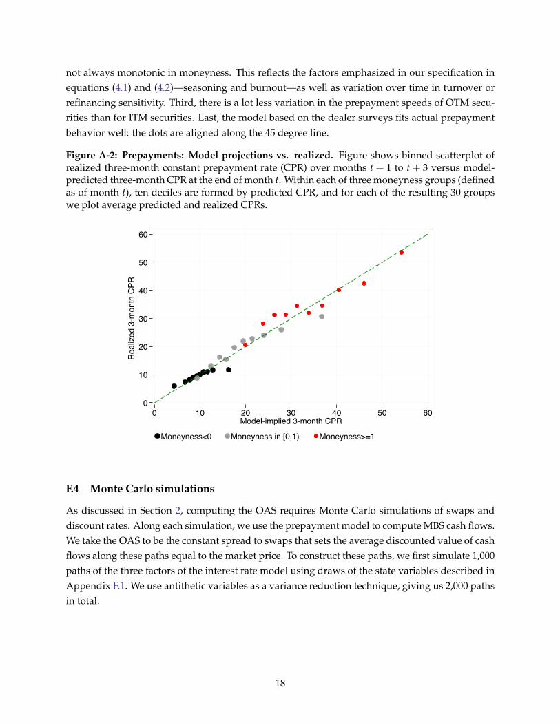
not always monotonic in moneyness. This reflects the factors emphasized in our specification inequations (4.1) and (4.2)—seasoning and burnout—as well as variation over time in turnover orrefinancing sensitivity. Third, there is a lot less variation in the prepayment speeds of OTM secu-rities than for ITM securities. Last, the model based on the dealer surveys fits actual prepaymentbehavior well: the dots are aligned along the 45 degree line.

Figure A-2: Prepayments: Model projections vs. realized. Figure shows binned scatterplot ofrealized three-month constant prepayment rate (CPR) over months t + 1 to t + 3 versus model-predicted three-month CPR at the end of month t. Within each of three moneyness groups (definedas of month t), ten deciles are formed by predicted CPR, and for each of the resulting 30 groupswe plot average predicted and realized CPRs.

0

10

20

30

40

50

60

Rea

lized

3-m

onth

CPR

0 10 20 30 40 50 60Model-implied 3-month CPR

Moneyness<0 Moneyness in [0,1) Moneyness>=1

F.4 Monte Carlo simulations

As discussed in Section 2, computing the OAS requires Monte Carlo simulations of swaps anddiscount rates. Along each simulation, we use the prepayment model to compute MBS cash flows.We take the OAS to be the constant spread to swaps that sets the average discounted value of cashflows along these paths equal to the market price. To construct these paths, we first simulate 1,000paths of the three factors of the interest rate model using draws of the state variables described inAppendix F.1. We use antithetic variables as a variance reduction technique, giving us 2,000 pathsin total.

18

G Identifying OASQ from the cross-section

In this Appendix, we relax the assumption that the risk-neutral prepayment function is a multipleof the physical prepayment function and explore identification of OASQ from the cross sectionof MBS. This alternative identification strategy relies on the cross section of stripped securitiesbeing priced fairly relative to each other at any given point in time, without requiring us to makeassumptions about the physical prepayment function.

In particular, we model the date τ risk-neutral single-monthly mortality (Q-SMM) rate of se-curity j as

sQj,τ = bQ

1 min(

Agejτ/30, 1

)+ κQ · f j

τ ·exp

(bQ

2 + bQ3 · INCj

τ

)1 + exp

(bQ

2 + bQ3 · INCj

τ

) ,

where INCjτ is the interest rate incentive to refinance and f j

τ is the “factor” (a pool’s remainingbalance relative to origination), at date τ. In this prepayment function we use the factor as a proxyfor the “burnout” effect; this is a simplified version of the specification in the main text. Mortgagerates have mostly trended lower in our sample and, absent the large volume of data from pre-payment surveys, one cannot separately identify empirically the effect of “burnout” (remainingborrowers are largely rate insensitive) from the effect of a lower sensitivity of all borrowers to rates(that would lead to the upper-flatness in the “S-shaped” prepayment function). In the simplifiedversion we assume that securities that exhibited more prepayments in the past (low f j

τ) tend toprepay more slowly, implying fewer parameters to be estimated than in the main text (χ and κ inequations (4.1) and (4.2) in Section 4.3).

For each pool j ∈ Jτ that trades at date τ, we compute the OAS implied by a set of pa-rameters

(bQ

1 , bQ2 , bQ

3 , κQ)

for the IO and the PO strip on that pool, denoted, respectively, by

OASj,IO

(bQ

1 , bQ2 , bQ

3 , κQ)

and OASj,PO

(bQ

1 , bQ2 , bQ

3 , κQ)

. At each date τ, we then minimize theremaining-principal-balance-weighted sum of the squared difference between OAS on the IO andthe PO strips written on the same pool:

arg min ∑j∈Jτ

θjτ

∑j∈Jτθjτ

(OASj,IO

(bQ

1 , bQ2 , bQ

3 , κQ)−OASj,PO

(bQ

1 , bQ2 , bQ

3 , κQ))2

, (G.1)

where θjτ is the remaining principal balance in pool j at date τ. The risk-neutral OAS on thepass-through security on pool j (the combination, denoted “PT,” of IO and PO) at date τ is thencomputed as the OAS implied by the set of parameters

(bQ

1 , bQ2 , bQ

3 , κQ)∗

that solves equation (G.1)at date τ:

OASQj ≡ OASj,PT

((bQ

1 , bQ2 , bQ

3 , κQ)∗)

.

This identification strategy relies on the assumption that the cross section of securities at a

19

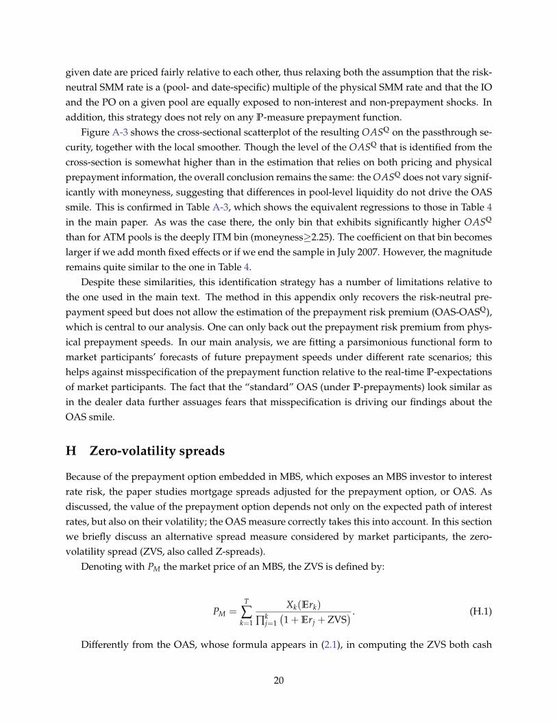
given date are priced fairly relative to each other, thus relaxing both the assumption that the risk-neutral SMM rate is a (pool- and date-specific) multiple of the physical SMM rate and that the IOand the PO on a given pool are equally exposed to non-interest and non-prepayment shocks. Inaddition, this strategy does not rely on any P-measure prepayment function.

Figure A-3 shows the cross-sectional scatterplot of the resulting OASQ on the passthrough se-curity, together with the local smoother. Though the level of the OASQ that is identified from thecross-section is somewhat higher than in the estimation that relies on both pricing and physicalprepayment information, the overall conclusion remains the same: the OASQ does not vary signif-icantly with moneyness, suggesting that differences in pool-level liquidity do not drive the OASsmile. This is confirmed in Table A-3, which shows the equivalent regressions to those in Table 4in the main paper. As was the case there, the only bin that exhibits significantly higher OASQ

than for ATM pools is the deeply ITM bin (moneyness≥2.25). The coefficient on that bin becomeslarger if we add month fixed effects or if we end the sample in July 2007. However, the magnituderemains quite similar to the one in Table 4.

Despite these similarities, this identification strategy has a number of limitations relative tothe one used in the main text. The method in this appendix only recovers the risk-neutral pre-payment speed but does not allow the estimation of the prepayment risk premium (OAS-OASQ),which is central to our analysis. One can only back out the prepayment risk premium from phys-ical prepayment speeds. In our main analysis, we are fitting a parsimonious functional form tomarket participants’ forecasts of future prepayment speeds under different rate scenarios; thishelps against misspecification of the prepayment function relative to the real-time P-expectationsof market participants. The fact that the “standard” OAS (under P-prepayments) look similar asin the dealer data further assuages fears that misspecification is driving our findings about theOAS smile.

H Zero-volatility spreads

Because of the prepayment option embedded in MBS, which exposes an MBS investor to interestrate risk, the paper studies mortgage spreads adjusted for the prepayment option, or OAS. Asdiscussed, the value of the prepayment option depends not only on the expected path of interestrates, but also on their volatility; the OAS measure correctly takes this into account. In this sectionwe briefly discuss an alternative spread measure considered by market participants, the zero-volatility spread (ZVS, also called Z-spreads).

Denoting with PM the market price of an MBS, the ZVS is defined by:

PM =T

∑k=1

Xk(Erk)

∏kj=1(1 + Erj + ZVS

) . (H.1)

Differently from the OAS, whose formula appears in (2.1), in computing the ZVS both cash

20

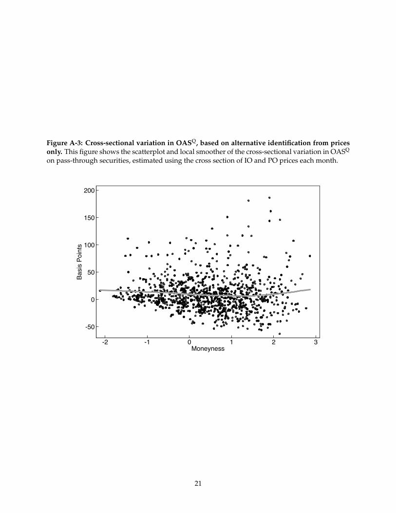
Figure A-3: Cross-sectional variation in OASQ, based on alternative identification from pricesonly. This figure shows the scatterplot and local smoother of the cross-sectional variation in OASQ

on pass-through securities, estimated using the cross section of IO and PO prices each month.

-50

0

50

100

150

200

Basi

s Po

ints

-2 -1 0 1 2 3Moneyness

21

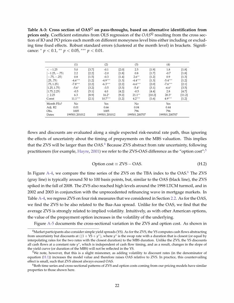
Table A-3: Cross section of OASQ on pass-throughs, based on alternative identification fromprices only. Coefficient estimates from OLS regression of the OASQ resulting from the cross sec-tion of IO and PO prices each month on different moneyness level bins either including or exclud-ing time fixed effects. Robust standard errors (clustered at the month level) in brackets. Signifi-cance: ∗ p < 0.1, ∗∗ p < 0.05, ∗∗∗ p < 0.01.

(1) (2) (3) (4)

< −1.25 5.0 [3.7] -0.1 [2.0] 2.5 [1.9] 1.8 [1.8][−1.25,−.75) 2.2 [2.2] -2.0 [1.8] 0.8 [1.7] -0.7 [1.8][−.75,−.25) 0.8 [1.5] -0.3 [1.4] 2.6∗∗ [1.2] 0.9 [1.3][.25, .75) -4.6∗∗∗ [1.2] -4.9∗∗∗ [1.3] -4.4∗∗∗ [1.3] -5.4∗∗∗ [1.2][.75, 1.25) -7.8∗∗∗ [2.2] -6.3∗∗∗ [2.2] -6.6∗∗∗ [2.0] -7.6∗∗∗ [2.1][1.25, 1.75) -5.6∗ [3.2] -3.5 [3.3] -5.4∗ [3.1] -6.6∗ [3.5][1.75, 2.25) -0.5 [5.1] 4.0 [4.2] -0.5 [4.4] 2.8 [4.7]≥ 2.25 6.3 [8.9] 16.2∗ [9.2] 21.1∗∗ [10.2] 20.3∗ [11.2]Const 11.1∗∗∗ [2.1] 10.7∗∗∗ [1.2] 4.2∗∗∗ [1.6] 4.9∗∗∗ [1.2]

Month FEs? No Yes No YesAdj. R2 0.01 0.66 0.04 0.44Obs. 1005 1005 796 796Dates 199501.201012 199501.201012 199501.200707 199501.200707

flows and discounts are evaluated along a single expected risk-neutral rate path, thus ignoringthe effects of uncertainty about the timing of prepayments on the MBS valuation. This impliesthat the ZVS will be larger than the OAS.4 Because ZVS abstract from rate uncertainty, followingpractitioners (for example, Hayre, 2001) we refer to the ZVS-OAS difference as the “option cost”:5

Option cost ≡ ZVS−OAS. (H.2)

In Figure A-4, we compare the time series of the ZVS on the TBA index to the OAS.6 The ZVS(gray line) is typically around 50 to 100 basis points, but, similar to the OAS (black line), the ZVSspiked in the fall of 2008. The ZVS also reached high levels around the 1998 LTCM turmoil, and in2002 and 2003 in conjunction with the unprecedented refinancing wave in mortgage markets. InTable A-4, we regress ZVS on four risk measures that we considered in Section 2.2. As for the OAS,we find the ZVS to be also related to the Baa-Aaa spread. Unlike for the OAS, we find that theaverage ZVS is strongly related to implied volatility. Intuitively, as with other American options,the value of the prepayment option increases in the volatility of the underlying.

Figure A-5 documents the cross-sectional variation in the ZVS and option cost. As shown in

4Market participants also consider simple yield spreads (YS). As for the ZVS, the YS computes cash flows abstractingfrom uncertainty but discounts at ((1 + YS + y∗), where y∗ is the swap rate with a duration that is closest (or equal byinterpolating rates for the two rates with the closest duration) to the MBS duration. Unlike the ZVS, the YS discountsall cash flows at a constant rate y∗, which is independent of cash flow timing, and as a result, changes in the slope ofthe yield curve (or duration of the MBS) will not be reflected in the YS.

5We note, however, that this is a slight misnomer, as adding volatility to discount rates (in the denominator ofequation (H.1)) increases the model value and therefore raises OAS relative to ZVS. In practice, this countervailingeffect is small, such that ZVS almost always exceed OAS.

6Both time series and cross-sectional patterns of ZVS and option costs coming from our pricing models have similarproperties to those shown here.

22

panel (b), ZVS are generally increasing in a contract’s moneyness, though the relation flattens outfor ITM securities. Panel (c) shows that the option cost (the difference between ZVS and OAS)is hump-shaped, with securities that are closest to par having the largest option cost. The humpshape of the option cost can be understood by analogy to the Vega (sensitivity to changes in thevolatility of the underlying) of vanilla call options, which is small for options that are deeply ITMor OTM but large for options near the money. Option execution in MBS are driven by an S-shapedprepayment function (rather than an exercise boundary) as discussed in more detail in Section 4.3but the patterns are analogous.7 As shown below, this pattern is directly related to the well-known“negative convexity” (i.e., concavity) of MBS prices with respect to rates, shown in panel (d): asrates drop (the security’s moneyness increases), prices increase less than linearly, especially fornear-the-money securities.

We conclude this section by briefly discussing an extension of the model from Section 3 thatfeatures interest rate uncertainty to discuss the cross-sectional variation in the option cost. Asdiscussed in Section 2, the option cost is reflected in the difference between the ZVS and the OAS,which with interest rate uncertainty can be shown to equal

ZVSt −OASt = −1Pt

∂2Pt

∂r2t

σ2r

2,

where σr is the volatility in the innovation in the interest rate diffusion. According to this ex-pression, the option cost is positive for negatively convex securities and is proportional to theGamma of the security (∂2Pt/∂r2

t ). Based on standard results in option pricing, Gamma is gener-ally greatest for at-the-money options and diminishes when moving either in or out of the money;furthermore, the option Vega, that is, its sensitivity to volatility, is directly related to its Gamma.This is consistent with the patterns shown in panels (c) and (d) of Figure A-5: option costs arelargest for ATM securities and prices are a concave function of moneyness (and therefore r).

7Intuitively, prepayments are not sensitive to small changes in interest rates when the prepayment option is deeplyITM or OTM, so that adding volatility to future interest rates matters little for the expected value of the security; thesame is not true for ATM securities.

23

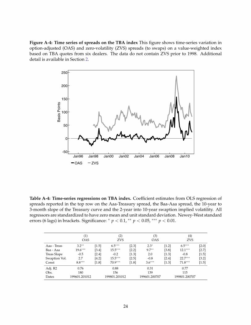
Figure A-4: Time series of spreads on the TBA index This figure shows time-series variation inoption-adjusted (OAS) and zero-volatility (ZVS) spreads (to swaps) on a value-weighted indexbased on TBA quotes from six dealers. The data do not contain ZVS prior to 1998. Additionaldetail is available in Section 2.

-50

0

50

100

150

200

250

Basis

Poi

nts

Jan96 Jan98 Jan00 Jan02 Jan04 Jan06 Jan08 Jan10

OAS ZVS

Table A-4: Time-series regressions on TBA index. Coefficient estimates from OLS regression ofspreads reported in the top row on the Aaa-Treasury spread, the Baa-Aaa spread, the 10-year to3-month slope of the Treasury curve and the 2-year into 10-year swaption implied volatility. Allregressors are standardized to have zero mean and unit standard deviation. Newey-West standarderrors (6 lags) in brackets. Significance: ∗ p < 0.1, ∗∗ p < 0.05, ∗∗∗ p < 0.01.

(1) (2) (3) (4)OAS ZVS OAS ZVS

Aaa - Treas 3.2∗∗ [1.5] 6.5∗∗∗ [2.3] 2.3∗ [1.2] 6.5∗∗∗ [2.0]Baa - Aaa 19.6∗∗∗ [3.4] 15.5∗∗∗ [2.2] 9.7∗∗ [3.8] 12.1∗∗∗ [2.7]Treas Slope -0.5 [2.4] -0.2 [1.3] 2.0 [1.3] -0.8 [1.5]Swaption Vol. 2.7 [4.2] 15.5∗∗∗ [2.5] -0.8 [2.4] 22.7∗∗∗ [3.2]Const 8.8∗∗∗ [1.8] 70.9∗∗∗ [1.8] 3.6∗∗∗ [1.3] 71.8∗∗∗ [1.5]

Adj. R2 0.76 0.88 0.31 0.77Obs. 180 156 139 115Dates 199601.201012 199801.201012 199601.200707 199801.200707

24

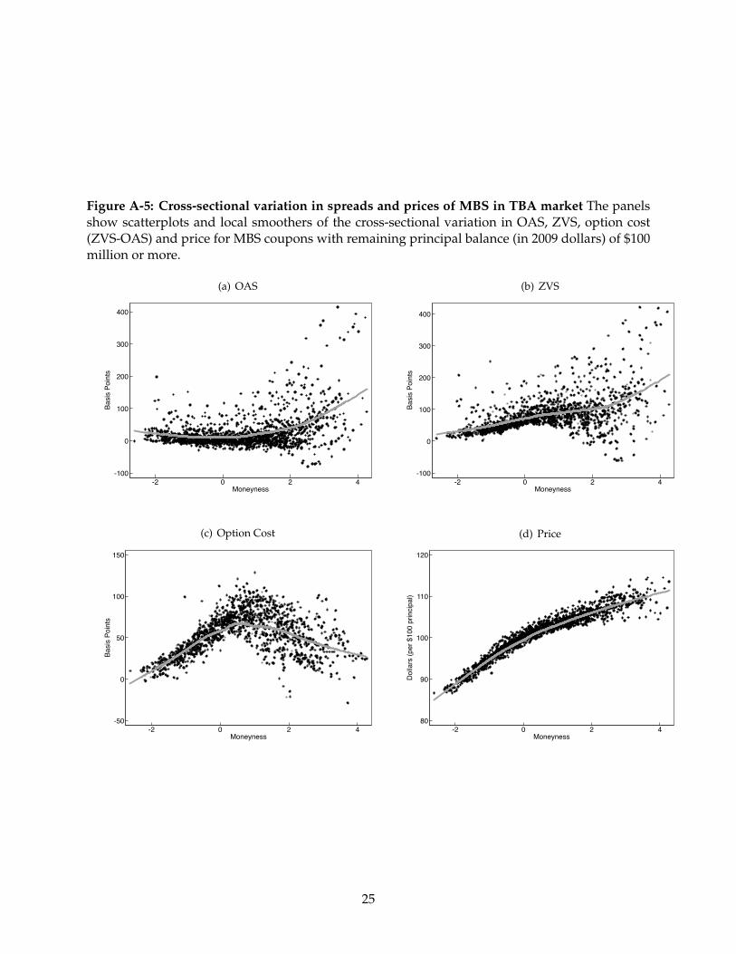
Figure A-5: Cross-sectional variation in spreads and prices of MBS in TBA market The panelsshow scatterplots and local smoothers of the cross-sectional variation in OAS, ZVS, option cost(ZVS-OAS) and price for MBS coupons with remaining principal balance (in 2009 dollars) of $100million or more.

(a) OAS

-100

0

100

200

300

400

Basi

s Po

ints

-2 0 2 4Moneyness

(b) ZVS

-100

0

100

200

300

400

Basi

s Po

ints

-2 0 2 4Moneyness

(c) Option Cost

-50

0

50

100

150

Basi

s Po

ints

-2 0 2 4Moneyness

(d) Price

80

90

100

110

120

Dol

lars

(per

$10

0 pr

inci

pal)

-2 0 2 4Moneyness

25