Mortgage Dollar Roll - Federal Reserve Bank of Atlanta

Mortgage Dollar Roll ∗

Zhaogang Song†

The Johns Hopkins Carey Business School

Haoxiang Zhu‡

MIT Sloan School of Management

February 3, 2016

Abstract

The most important financing strategy of agency MBS – mortgage dollar roll – is a

secured lending contract with the unique feature that returned MBS collateral can

differ from those received, creating adverse selection for the cash borrower. Using

a proprietary dataset, we provide the first analysis of dollar roll “specialness”, the

extent to which implied dollar roll financing rates fall below prevailing market rates.

Dollar roll specialness increases in adverse selection and decreases in MBS liquidity.

Specialness is also negatively related to expected MBS returns. Moreover, the Federal

Reserve’s MBS purchases and dollar roll sales are associated with lower specialness.

Keywords: Dollar Roll, TBA, MBS, Specialness, LSAP

JEL classification: G12, G18, G21, E58

∗First version: January 2014. We thank helpful comments from James Vickery, Joyner Edmundson, KatyFemia, Song Han, Jean Helwege, Jeff Huther, Bob Jarrow, Matt Jozoff, Akash Kanojia, Ira Kawaller, BethKlee, Arvind Krishnamurthy, Guohua Li, Debbie Lucas, Jessica Lynch, Nicholas Maciunas, Tim McQuade,John Miller, Linsey Molloy, Danny Newman, Greg Powell, Bernd Schlusche, Hui Shan, Andrea Vedolin,Clara Vega, Min Wei, and seminar participants at the Third Annual Fixed Income Conference, the 2015FIRS conference, Cornell University, Shanghai Advanced Institute of Finance (SAIF), and the 2015 FederalReserve Bank of Atlanta Real Estate Finance Conference.†The Johns Hopkins Carey Business School, 100 International Drive, Baltimore, MD 21202. E-mail:

[email protected].‡MIT Sloan School of Management, 100 Main Street E62-623, Cambridge, MA 02142. [email protected].

Mortgage Dollar Roll

February 3, 2016

Abstract

The most important financing strategy of agency MBS – mortgage dollar roll – is a

secured lending contract with the unique feature that returned MBS collateral can

differ from those received, creating adverse selection for the cash borrower. Using

a proprietary dataset, we provide the first analysis of dollar roll “specialness”, the

extent to which implied dollar roll financing rates fall below prevailing market rates.

Dollar roll specialness increases in adverse selection and decreases in MBS liquidity.

Specialness is also negatively related to expected MBS returns. Moreover, the Federal

Reserve’s MBS purchases and dollar roll sales are associated with lower specialness.

1 Introduction

“The Federal Reserve Bank of New York on Tuesday said it has been conducting a type

of mortgage-bond-repurchase transaction to aid the earlier settlement of its outstanding

mortgage-backed securities purchases, which is supporting the larger market. In purchas-

ing the dollar rolls, the Fed could be relieving liquidity bottlenecks for investors who need

to borrow a security they are short but have contracted to deliver to a buyer...”

—The Wall Street Journal, December 6, 2011

This paper provides an empirical analysis of the funding market of agency mortgage-

backed-securities (MBS). A better understanding of this market is important because of

its large size and its tight connection to the implementation of unconventional monetary

policy in the United States, as we elaborate below. Analyzing the MBS funding market

also provides unique economic insights that are absent in the repo markets of fixed-income

securities.

Agency MBS guaranteed by Ginnie Mae (GNMA), Fannie Mae (FNMA), and Freddie

Mac (FHLM) form a major component of U.S. fixed-income markets.1,2 According to SIFMA,

as of the third quarter of 2015, the outstanding amount of agency MBS is about $7.14 trillion,

which is more than a half of the outstanding $12.84 trillion of U.S. Treasury securities. The

average daily trading volume of agency MBS is 20 times larger than that of corporate bonds,

and close to 60% of that for Treasury securities in 2010, according to Vickery and Wright

(2011).

Besides its large size and trading volume, the agency MBS market also plays a prominent

role in the implementation of U.S. monetary policy since the global financial crisis. The

Federal Reserve has conducted several rounds of quantitative easing (QE) since 2009 and

accumulated $1.74 trillion face value of agency MBS on its balance sheet as of January 2015.

Furthermore, the Federal Open Market Committee has announced in its September 2014

statement that the Federal Reserve will continue to use its MBS holdings to conduct reverse

1Throughout the paper, the term MBS refers only to residential mortgage-backed-securities rather thanthose backed by commercial mortgages, unless otherwise noted.

2Ginnie Mae, Fannie Mae, and Freddie Mac stand for the Government National Mortgage Association,Federal National Mortgage Association, and Federal Home Loan Mortgage Corporation, respectively. GinnieMae is a wholly-owned government corporation within the Department of Housing and Urban Development.Usually called Government-Sponsored Enterprises (GSEs), Fannie Mae and Freddie Mac were private entitieswith close ties to the U.S. government before September 2008, and have been placed in conservatorship bythe Federal Housing Financing Agency and supported by the U.S. Treasury department since then.

1

repo transactions as a regular policy tool in the future (see Frost, Logan, Martin, McCabe,

Natalucci, and Remache (2015)).

About a half of the trading volume in the entire agency MBS market is conducted through

a type of strategy called (mortgage) “dollar roll”, the most widely used mechanism by which

investors finance their positions in agency MBS and hedge their existing MBS exposures

(Gao, Schultz, and Song (2015)). It is also a particularly important tool that the Federal

Reserve uses actively in its operations of quantitative easing (see the Wall Street Journal

quote above). Specifically, a mortgage dollar roll is the combination of two forward contracts

on MBS, one front month and one future month. These forward contracts are traded in the

liquid “to-be-announced” (TBA) market, which comprises over 90% of agency MBS trading

volume and all the Federal Reserve’s MBS purchases. In a dollar roll transaction the “roll

seller” sells an MBS in the front-month TBA contract and simultaneously buys an MBS in

the future-month TBA contract, both at specified prices. A roll buyer does the opposite.

A unique feature of the TBA market is that, on the trade date, the two counterparties

only agree on generic security characteristics, such as agency, coupon, and original mortgage

term, but not the specific CUSIPs to be delivered. A dollar roll, as a combination of two TBA

trades, inherits this important feature. For example, a particular dollar roll contract may

specify that the deliverable MBS must be guaranteed by Fannie Mae, with the original loan

term of 30 years and a coupon rate of 4% per year. But on the trade date it does not specify

the particular CUSIP of MBS to be delivered. Thus, the short side has a strong incentive

to deliver the cheapest CUSIP that satisfy these parameters, creating adverse selection for

the long side. In particular, after the roll seller delivers an MBS in the front month of a

dollar roll, he may (and is likely to) receive a different, potentially inferior MBS in the future

month.3 This adverse-selection risk is reflected by the prices in the two legs of the dollar

roll.

It is convenient and intuitive to view a dollar roll as a collateralized borrowing contract,

with the roll seller being the cash borrower. Compared to a standard repo contract, however,

the roll seller faces a substantial risk that the collateral redelivered at the end of the contract

are inferior to the original collateral lent out. To compensate for this risk, the roll seller,

equivalently the cash borrower, pays a low and sometimes even negative implied financing

3The roll buyer is also subject to this adverse-selection risk between the trade date and the front-monthsettlement date. We expect this risk to be limited because (1) the roll buyer has the last say on thedelivered CUSIP, and (2) the roll trade date is usually close to the front-month settlement date when bothcounterparties have a good idea on the cheapest MBS in practice. See Section 3 and Section 4 for detaileddiscussions.

2

rate. A dollar roll is said to be “on special” if this implied financing rate is lower than the

prevailing market interest rate, such as the general-collateral (GC) repo rate on the MBS

or unsecured rates like LIBOR. The specialness of a dollar roll is hence a key indicator of

funding conditions in agency MBS markets, just as repo specialness is a key indicator of

funding conditions in U.S. Treasury markets.

To the best of our knowledge, this paper provides the first analysis of the economics of

dollar roll specialness. We ask the following three questions:

1. What economic forces determine dollar roll specialness?

2. What is the relation between dollar roll specialness and the expected MBS returns?

3. How does the Federal Reserve’s large-scale asset purchase of agency MBS affect dollar

roll specialness, and through which channels?

Answers to these questions would shed light on this important yet underexplored market

in the academic literature. It also provides new evidence on the effect of unconventional

monetary policy on market functioning.

Our analysis starts with an analytic framework that encompasses two important deter-

minants of dollar roll specialness. The first is associated with the key feature of a dollar roll

transaction: securities changing hands in the two legs of a dollar roll need not be the same,

but only “substantially similar,” as defined by a set of parameters.4 We call the collection

of MBS CUSIPs that satisfy a particular set of parameters a “cohort.” Therefore, the roll

buyer can potentially (and generally will) deliver the cheapest MBS within a cohort to the

roll seller (the cheapest-to-deliver (CTD) option). An agency MBS is cheap mainly because

it has inferior prepayment characteristics not specified in the TBA contract, such as the

loan-to-value ratio, FICO score, past prepayment behavior, and location of the mortgage,

relative to other agency MBS in the same cohort.5 (The default risk is insured by the agen-

cies.) This adverse selection lowers the interest rate that the roll seller is willing to pay

and hence increases specialness. We illustrate the adverse-selection channel in a simple and

stylized model.

4The criterion of “substantially similar” is defined in the American Institute of Certified Public Accoun-tants State of Position 90-3 such that the original and returned MBS should be of the same agency, originalloan term, and coupon rate, and both should satisfy Good Delivery requirement set by SIFMA.

5We emphasize that inferior prepayment characteristics do not necessarily mean higher prepaymentspeeds. A high prepayment speed usually implies a low value for a premium MBS with value above par,but a high value for a discount MBS with value below par (See Section 3 for details). Hence, MBS withinferior prepayment characteristics refer to those with high (low) prepayment speeds if the correspondingTBA cohort is at premium (discount).

3

The second determinant of dollar roll specialness is a liquidity channel associated with

search frictions, motivated from the literature on over-the-counter markets.6 Specifically,

if MBS supply for dollar roll trading is scarce, it is more costly for roll buyers to locate

these MBS due to search frictions. Roll sellers who hold the scarce MBS would be in a

more advantageous bargaining position than roll buyers. Hence, the buyer has to offer lower

financing rates, which will lead to a higher specialness.

Based on this analytic framework, we empirically study dollar roll specialness using two

proprietary data sets. The first data set includes the dollar roll financing rates, option-

adjusted spreads, and single-month mortality rates of FNMA 30-year TBA contracts with

twelve coupon rates ranging from 3% to 8.5% at the daily frequency over July 2000 – July

2013, provided by J.P. Morgan. We calculate dollar roll specialness as the difference between

prevailing one-month interest rates, such as the 1-month general collateral repo rate of agency

MBS or the 1-month LIBOR, and the dollar roll financing rates. From these daily time series

we construct monthly series of specialness and other variables. The second data set includes

the characteristics data of all FNMA 30-year MBS CUSIPs at the monthly frequency over

July 2005 – July 2013, provided by eMBS.

Our empirical investigation consists of three parts, corresponding to the three questions

above.

Determinants of dollar roll specialness. Our analytic framework reveals two important

determinants of dollar roll specialness: adverse selection and liquidity. Our simple model

suggests that the adverse-selection channel is closely linked to the expected cohort-level

prepayment speed: a higher prepayment speed will lead to a larger heterogeneity of MBS

values within the TBA cohort and hence a lower value of the cheapest-to-deliver (CTD)

MBS relative to the original collateral. We measure the cohort-level prepayment speed by

the widely-used single monthly mortality rate (SMM) (see Hayre (2001)). Our analytic

framework also suggests that dollar roll specialness should decrease in the liquidity of MBS

market. We proxy liquidity by constructing a measure of the net supply of CTD MBS

CUSIPs, labeled NSupplyCTD. Specifically, starting from the universe of all CUSIPs of a

coupon cohort, we eliminate CUSIPs whose characteristics make prepayment unlikely (using

criteria similar to those used by Himmelberg, Young, Shan, and Henson (2013)), and then

6This liquidity channel is consistent with search theories of Duffie, Garleanu, and Pedersen (2002) andVayanos and Weill (2008) as well as evidence regarding repo specials and on-the-run premium in Treasurymarkets (see Jordan and Jordan (1997), Krishnamurthy (2002), and Graveline and McBrady (2011), amongothers).

4

sum up the outstanding amount of remaining CUSIPs to construct a raw measure of the

supply of CTD cohort. Then we deduct the deal volume of collateralized mortgage obligations

(CMOs) from the raw supply measure to get a measure of net supply of CTD cohort.7

We test how adverse selection and liquidity affect dollar roll specialness in panel regres-

sions. Confirming the predictions from our analytic framework, a higher prepayment speed

(SMM) is associated with higher specialness, and a higher CTD supply (NSupplyCTD) is

associated with a lower specialness. The economic magnitudes are also large. In particular,

a one standard deviation increase in SMM increases dollar roll specialness by about 20

basis points, whereas a one standard deviation increase in NSupplyCTD decreases special-

ness by 18 basis points. The significance of these variables is robust to alternative model

specifications.8

Dollar roll specialness and expected MBS returns. Because a higher specialness

implies a lower financing cost, we expect that owners of MBS that are on special are willing

to accept lower expected returns from these MBS. That is, we expect a negative specialness-

expected return relation. Following Gabaix, Krishnamurthy, and Vigneron (2007), we use

the option-adjusted spreads (OAS) as a proxy for expected MBS returns. The OAS is the

yield on an MBS in excess of the term structure of interest rates after adjusting for the

expected value of homeowners’ prepayment options, conditional on the interest rate path.

Using monthly OAS for the same collection of FNMA 30-year TBA contracts, we find a

pronounced negative relation between OAS and dollar roll specialness. In particular, an MBS

cohort that is on special has an OAS that is about 60 basis points lower than that of an MBS

cohort not on special, controlling for coupon and time fixed effects. A one percentage point

increase in specialness is associated with an OAS that is about 45 basis points lower. As a

robustness check, we use the the realized returns of rolling TBA contracts as an alternative

proxy for expected MBS returns, and also find a strong negative relation between specialness

and expected MBS returns. These results are robust to a variety of empirical specifications.

The effect of LSAP on dollar roll specialness. As one of the most important central

bank actions since the 2008 financial crisis, the large MBS purchase by the Fed raises potential

concerns of market distortion. As highlighted by Bernanke (2012), “Conceivably, if the

7We are grateful to John Miller for suggesting the agency CMO data on Bloomberg.8These specifications include whether the GC repo rate or LIBOR is used to measure specialness and

whether the activeness of the TBA coupon buckets is adjusted. We also obtained similar results using theBarclays data of dollar roll financing rates.

5

Federal Reserve became too dominant a buyer in certain segments of these markets, trading

among private agents could dry up, degrading liquidity and price discovery.”

We find that regressing dollar roll specialness on Fed purchases leads to a negative coef-

ficient. While this negative relation suggests that the large size of MBS absorbed by the Fed

does not result in (detectable) market distortions, we cautiously interpret it as correlation,

rather than causality, because we do not have an exogenous shock to LSAP. That said, we

conduct two empirical tests that provide suggestive evidence on how the Fed’s transactions

in MBS markets may affect specialness. First, the inclusion of SMM and NSupplyCTD in

the specialness-LSAP regression reduces the magnitude of the negative coefficient on LSAP,

suggesting that Fed purchases do interact with adverse selection and supply channels in MBS

markets. Second, we find that the Fed conducts more dollar roll sales in coupon cohorts with

higher LSAP purchases and lower specialness, suggesting that the Fed attempts to alleviate

(real or perceived) squeezes in MBS market by delaying taking delivery of the purchased

MBS.

Relation to the literature. To the best our knowledge, this paper is the first academic

study of dollar roll specialness. It contributes to three branches of literature: MBS markets,

repo specialness, and the effects of the Federal Reserve’s asset purchases.

The prior literature on MBS market has predominantly focused on the pricing of MBS.

We focus on the financing of MBS. (This difference is analogous to the difference between the

pricing of Treasury securities and the financing of them through repo transactions.) Studies

on the pricing of MBS include Dunn and McConnell (1981), Schwartz and Torous (1989),

Stanton (1995), Boudoukh, Richardson, Stanton, and Whitelaw (1997), and Kupiec and Kah

(1999), among others. Several recent studies, Gabaix, Krishnamurthy, and Vigneron (2007),

Duarte, Longstaff, and Yu (2007), Chernov, Dunn, and Longstaff (2015), and Boyarchenko,

Fuster, and Lucca (2015) investigate the return patterns of MBS, but they do not connect

these return patterns to dollar roll specialness or systematically analyze the determinants

of specialness.9 A recent expanding literature studies the market structure and liquidity of

the agency MBS market, including Atanasov and Merrick (2012), Atanasov, Merrick, and

Schuster (2014), Bessembinder, Maxwell, and Venkataraman (2013), Downing, Jaffee, and

Wallace (2009), Friewald, Jankowitsch, and Subrahmanyam (2014), Gao, Schultz, and Song

(2015), and Hollifield, Neklyudov, and Spatt (2014).10 Dollar roll specialness is not the focus

9Two other recent studies, Malkhozov, Mueller, Vedolin, and Venter (2013) and Hansen (2014), showthat variables capturing the mortgage risk hedging have return predictive power for Treasury bonds.

10After our paper has been widely distributed in January 2014, a very recent paper Kitsul and Ochoa

6

of any of these studies.

Our study is also related to the literature on special repo rates in Treasury markets,

including Duffie (1996), Jordan and Jordan (1997), Buraschi and Menini (2002), Krish-

namurthy (2002), Duffie, Garleanu, and Pedersen (2002), Cherian, Jacquier, and Jarrow

(2004), Vayanos and Weill (2008), Pasquariello and Vega (2009), and Banerjee and Grave-

line (2013), among others. The economics of dollar roll specialness in agency MBS markets

differs substantially from that of Treasury repo specialness in that a dollar roll involves a

major adverse-selection risk that an inferior security is returned. Adverse selection is a key

determinant of dollar roll specialness.

Lastly, our analysis of the impact of LSAP on dollar roll specialness relates to Hancock

and Passmore (2011), Gagnon, Raskin, Remanche, and Sack (2011), Krishnamurthy and

Vissing-Jorgensen (2011), Krishnamurthy and Vissing-Jorgensen (2013), and Stroebel and

Taylor (2012), who analyze the effect of LSAP on mortgage rates. Among these, Krish-

namurthy and Vissing-Jorgensen (2013) highlight the importance of the cheapest-to-deliver

option in TBA markets. Complementary to these studies that focus on the level of mortgage

rates, we investigate the impact of LSAP on MBS funding markets. Kandrac (2013) finds

that LSAP is associated with a lower dollar roll implied financing rates, which is also about

the level of (collateralized) interest rate. He neither studies the determinants of dollar roll

specialness nor link the two channels of specialness to LSAP. Our analysis fills this important

gap.

2 TBA Market and Dollar Roll

This section discusses institutional details of the TBA trading convention in agency MBS

markets and dollar roll transactions, which consist of two simultaneous TBA trades (see

Hayre (2001) and Hayre and Young (2004) for detailed industry references of MBS mar-

kets).11 A worked-out example for the computation of dollar roll financing rates are provided

in Appendix.

(2014) conducted some similar analyses.11All TBA-eligible MBS are so-called “pass-through” securities, which pass through the monthly principal

and interest payments less a service fee from a pool of mortgage loans to owners of the MBS. Structuredmortgage-backed-securities like CMOs, which tranche mortgage cash flows with various prepayment andmaturity profiles, are not eligible for delivery in TBA contracts.

7

2.1 TBA market

A TBA contract is essentially a forward contract to buy or sell an MBS. In a TBA trade,

the buyer and seller negotiate on six general parameters: agency, maturity, coupon rate,

par amount, price, and settlement date. Different from other forward contracts, there is

only one settlement date per month for TBA contracts, set by SIFMA. For example, for

30-year FNMA MBS, the settlement day is usually the 12th or 13th of the month. A single

settlement date per month concentrates liquidity.

We now demonstrate the trading procedure in TBA markets through a concrete and

hypothetical example, illustrated in Figure 1.

Figure 1: A TBA Example

• Trade and Confirmation Dates. On the trade date April 25, the buyer and seller

decide on the six trade parameters. In this example, a TBA contract is initiated on April 25

and will be settled on May 16. The seller can deliver any MBS issued by Fannie Mae with

the original mortgage loan term of 30 years, annual coupon rate of 5%, par amount of $1

million, and price at $(102+16/32) per $100 of par amount. The trade is confirmed within

one business day, which in this case is April 26.

• 48-Hour Day. The seller notifies the buyer the actual identity (i.e., the CUSIPs) of

the MBS to be delivered on the settlement date, no later than 3 p.m. two business days prior

8

to the settlement date (“48-hour day”), which is May 14 in the example. These MBS pools

have to satisfy the “Good Delivery” requirements set by SIFMA. For example, for each $1

million lot, the contract allows a maximum of three pools to be delivered and a maximum

0.01% difference in the face value; that is, the sum of the par amounts of the pools can

deviate from $1 million by no more than $100 in either direction.

• Settlement Date. The seller delivers the MBS pools specified on the 48-hour day,

and the buyer pays an amount of cash equal to the current face value times the TBA price

(i.e., 102-16 in this example) plus accrued interests from the beginning of the month, given

that the seller holds the MBS pools until the settlement date. Accrued interest is computed

on a 30/360 basis. There is one settlement date for a type of TBA contract in each month,

fixed by SIFMA. For example, FNMA and FHLM 30-year TBA trades settle on the same

Class A schedule that typically falls around the 12th or 13th of each month (Gao, Schultz,

and Song (2015)).

The unique feature of a TBA trade is that the actual identity of the MBS to be delivered

at settlement date is not specified on the TBA trade date. By specifying only a few key

MBS characteristics, this TBA trading design dramatically increases the set of deliverable

MBS and substantially improves market liquidity.

2.2 Dollar roll

A dollar roll transaction consists of two TBA trades. The “roll seller” sells an MBS in

the front month TBA contract and simultaneously buys an MBS in the future month TBA

contract with the same TBA characteristics, at specified prices. In particular, the two MBS

delivered into the two TBA contracts need not have the same CUSIP, as long as they have

the same TBA characteristics.

Figure 2 shows the time line of an example dollar roll trade. In this example, the roll

seller sells an MBS for May 16 settlement and buys it back for June 16 settlement, for a par

amount of $1 million Fannie Mae MBS with the original loan term of 30 years and annual

coupon rate of 5%, and with the front and future month prices at 102-16 and 102-2 per $100

of par amount, respectively.

The “drop” of this dollar roll, defined as the price difference between the front- and

future-month TBA contracts, is positive for two reasons. (In this example, the drop is

1001632−100 2

32= 14

32per $100 par value.) First, and most importantly, the returned MBS pool

in the future-month TBA contract may have inferior prepayment behavior and hence lower

value than the original MBS sold in the front-month contract. Second, after the front-month

9

leg of the dollar roll transaction, the roll seller gives up the ownership of the MBS and any

interest and principal payments. These two features, especially the redelivery uncertainty of

the returned MBS pool in the future-month leg, differentiates the dollar roll from an MBS

repo transaction. In an MBS repo trade the same MBS pool has to be returned, and the

original owner collects principal and interest payments during the term of repo.12

Figure 2: A Dollar Roll Example

A dollar roll can be viewed as a collateralized borrowing contract, with the important fea-

ture that the returned collateral can differ from the original collateral. As in repo contracts,

we can calculate the effective collateralized borrowing rate for dollar roll transactions. The

borrowing rate of a dollar roll, which measures the benefit of rolling an MBS pool relative to

holding it, can be computed based on the drop after adjusting for the principal and coupon

payments the roll seller gives up over the roll period. As an over-simplified example, suppose

that the front-month and future-month prices of the dollar roll transactions are P0 and P1,

respectively, and the coupon and principal payments of the MBS received by the roll buyer

12Additionally, the cash lender in a repo transaction is generally able to call margin from the cash borrowerperiodically (as often as daily), protecting the lender against counterparty risk associated with fluctuationsin the underlying collateral value.

10

are c and d, respectively. Then, the effective financing rate of the dollar roll is

r =P1 + c+ d

P0

− 1. (1)

A worked example of calculating dollar roll specialness is provided in the Appendix.

Participants in the TBA and dollar roll markets include MBS dealers, mortgage servicers,

pension funds, mutual funds, endowments, hedge funds, commercial banks, and insurance

companies. The Federal Reserve and foreign central banks with large dollar reserves (e.g.

China and Japan) sometimes participate in MBS markets as well. Among them, commer-

cial banks, insurance companies, and pension funds mostly use buy-and-hold strategies and

only trade dollar rolls occasionally, due to accounting considerations. Much of the dollar

roll demand comes from MBS dealers who need to cover their short MBS hedging trades or

maintain their MBS inventories for market-making.13 Mortgage servicers and money man-

agers are main providers of dollar rolls, with the former enhancing their portfolios returns at

desirable financing rates and the latter financing their MBS positions to hedge their interest

rate exposure of the loans they service on their books. Hedge funds demand or supply dollar

rolls for both hedging and speculation.

2.3 Dollar roll specialness

We say a dollar roll is “on special” if the implied finance rate is lower than the prevailing

interest rates, such as MBS repo rates or LIBOR. The specialness of a dollar roll, defined as

the market prevailing borrowing rate less the implied finance rate in a dollar roll, provides

a rent to the MBS owners and represents an effective reduction in the financing costs of

MBS positions. A positive specialness, however, is not an arbitrage in any sense, as the

dollar roll seller bears the redelivery risk, i.e., the risk of an MBS with inferior prepayment

characteristics being returned in the future-month TBA contract. The higher is the risk,

the lower price the roll seller is willing to offer in the future month of the dollar roll, and

the lower is the implied financing rate (see equation (1) and the example in the previous

subsection). Hence, specialness is higher. In other words, a positive dollar roll specialness is

a compensation for the roll seller for taking the redelivery risk.

To see the intuition more clearly, we consider this stylized example. Suppose that the

implied dollar roll financing rate on an MBS (and other MBS in the same cohort) is −1%,

13Dealers’ short positions in MBS could be hedges against their long positions in CMOs, specified pools,certain non-agency MBS, or bonds they have purchased for delivery in future months from originators.

11

but the repo rate of using this specific MBS for secured borrowing is 2%. An investor with

$1 million cash can engage in the following trades. She lends the cash against the MBS in

the repo market for one month at 2%, and subsequently rolling the MBS collateral for one

month at the financing rate of −1%. If, by any chance, the same MBS is returned to the

investor in the dollar roll market, she can return the same MBS to the repo counterparty and

close the repo contract; this earns her the net profit of $(2%+1%)/12 million. If, however, a

different and cheaper MBS is returned in the dollar roll contract, this different MBS cannot

be used to close the repo contract, and she must buy or borrow the original MBS to close the

repo contract. In this process, she must make up for the price difference between the original

MBS and cheaper MBS delivered back in the dollar roll. The specialness of 3% (relative to

MBS repo rate), therefore, compensates for such risks borne by the roll seller.

In addition to being a compensation for adverse selection stemming from redelivery risk,

dollar roll specialness also reflects the general supply and demand conditions in the TBA

market. For example, if the MBS of particular characteristics are scarce in the market, a

holder of such MBS can extract more rents in the repo market and security lending market.

By rolling this MBS, the roll seller gives up not only the interest and principal payments,

but also the rents associated with cheaper financing rates and lending fees. Therefore, the

equilibrium implied financing rate in the dollar roll must fall, leading to a higher specialness.

The scarcity of a particular class of MBS can be driven by the shorting and hedging activities

of dealers and originators, as well as the amounts of newly issued MBS.

3 The Economics of Dollar Roll Specialness

In this section we develop an analytic framework to study the economics of dollar roll spe-

cialness. We consider first the determinant of dollar roll specialness and then the relation

between dollar roll specialness and expected MBS returns.

3.1 The determinants of dollar roll specialness

In this subsection we focus on two determinants of dollar roll specialness: adverse selection

and liquidity. A few additional considerations—including prepayment risk borne by the roll

buyer, default risk, and settlement failures—are discussed and tested in Section 8.

12

3.1.1 Redelivery risk and adverse selection

As we discussed in the previous section, a key feature of financing MBS by dollar roll, relative

to financing by repo, is that the roll buyer (who lends cash and receives an MBS) has the

option to deliver a substantially similar but different MBS in the future month of the roll

contract. As a compensation, the roll seller offers a lower price to buy back the substantially

similar MBS in the future-month leg. This low price, in turn, implies a lower effective

financing rate, or a higher specialness.

To illustrate the formal link between dollar roll specialness and adverse selection imbed-

ded in dollar roll contracts, we consider the following simple, stylized model.

There are three periods, t ∈ {0, 1, 2}. The discount rate is r per period. Multiple MBS

CUSIPs of the same cohort, indexed by i ∈ {1, 2, . . . , n}, trade in the market. Investors

are risk-neutral. For simplicity, suppose that all MBS have the same coupon rate c > 0

and maturity at t = 2. These MBS, however, have heterogeneous prepayment speeds. In

particular, for MBS i, a random fraction λi of the underlying mortgages will be prepaid at

t = 1 and the remaining fraction 1−λi will be paid at t = 2. This information is unobservable

ex ante. Thus, the time-0 value of a generic MBS is

P0 = E[λi

1 + c

1 + r+ (1− λi)

(c

1 + r+

1 + c

(1 + r)2

)]=

c

1 + r+

1 + c

(1 + r)2− c− r

(1 + r)2E[λi]. (2)

If c > r, prepayment lowers (premium) MBS value; if c < r, prepayment increases (dis-

count) MBS value. Suppose that strictly between t = 0 and t = 1 all {λi} become public

information.

Now consider a dollar roll contract transacted at time t = 0. For simplicity, suppose that

the front-month leg is settled at t = 0 and the future-month leg is settled at t = 1. One

may worry that such a dollar roll schedule abstracts away from the uncertainty faced by the

roll buyer regarding the value of the MBS collateral because the transaction date and the

front-month settlement date are not necessarily the same in reality. In fact, however, this

uncertainty is limited in reality because most of the dollar roll transactions happen shortly

before the front-month settlement date when investors (both sellers and buyers of the dollar

roll) have a good idea about what CUSIPs constitute the cheapest-to-deliver cohort.

Also for simplicity and to focus on the adverse selection channel, suppose that the MBS

13

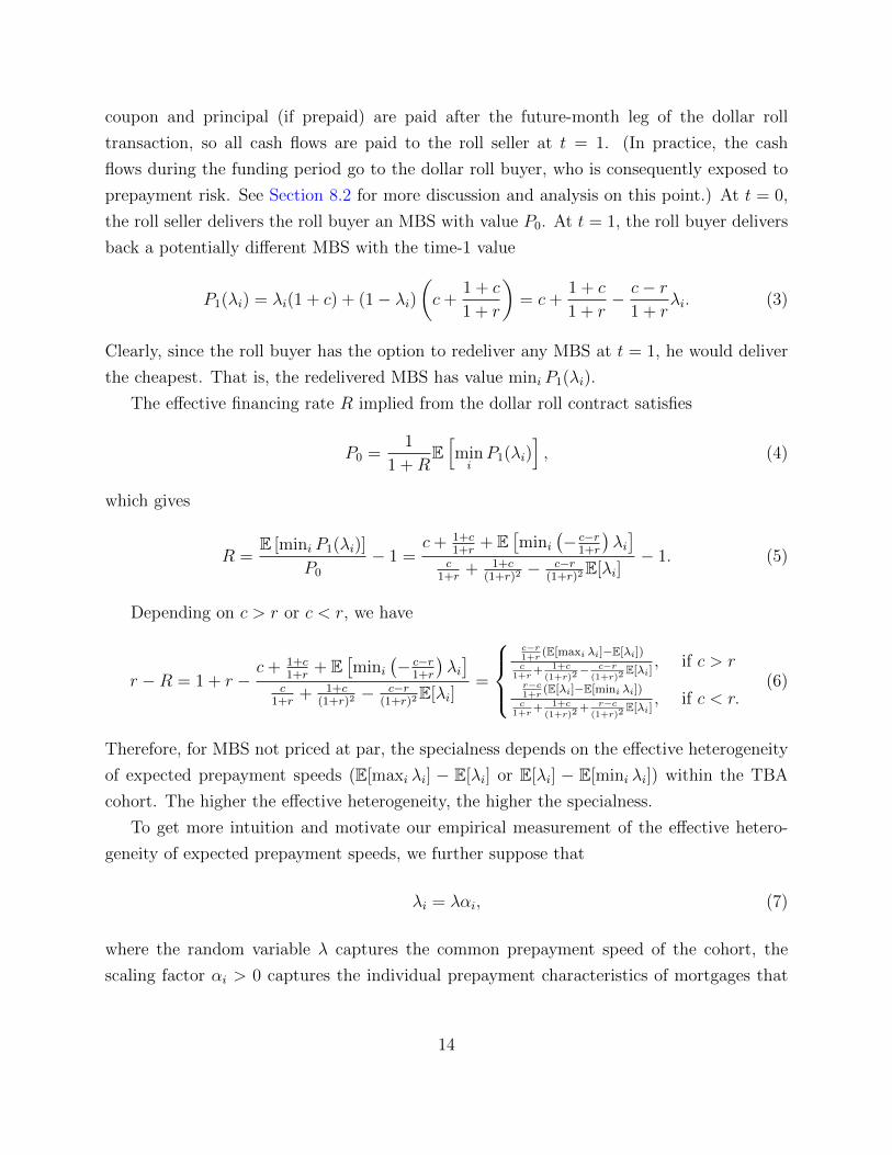
coupon and principal (if prepaid) are paid after the future-month leg of the dollar roll

transaction, so all cash flows are paid to the roll seller at t = 1. (In practice, the cash

flows during the funding period go to the dollar roll buyer, who is consequently exposed to

prepayment risk. See Section 8.2 for more discussion and analysis on this point.) At t = 0,

the roll seller delivers the roll buyer an MBS with value P0. At t = 1, the roll buyer delivers

back a potentially different MBS with the time-1 value

P1(λi) = λi(1 + c) + (1− λi)(c+

1 + c

1 + r

)= c+

1 + c

1 + r− c− r

1 + rλi. (3)

Clearly, since the roll buyer has the option to redeliver any MBS at t = 1, he would deliver

the cheapest. That is, the redelivered MBS has value mini P1(λi).

The effective financing rate R implied from the dollar roll contract satisfies

P0 =1

1 +RE[miniP1(λi)

], (4)

which gives

R =E [mini P1(λi)]

P0

− 1 =c+ 1+c

1+r+ E

[mini

(− c−r

1+r

)λi]

c1+r

+ 1+c(1+r)2

− c−r(1+r)2

E[λi]− 1. (5)

Depending on c > r or c < r, we have

r −R = 1 + r −c+ 1+c

1+r+ E

[mini

(− c−r

1+r

)λi]

c1+r

+ 1+c(1+r)2

− c−r(1+r)2

E[λi]=

c−r1+r

(E[maxi λi]−E[λi])c

1+r+ 1+c

(1+r)2− c−r

(1+r)2E[λi]

, if c > rr−c1+r

(E[λi]−E[mini λi])c

1+r+ 1+c

(1+r)2+ r−c

(1+r)2E[λi]

, if c < r.(6)

Therefore, for MBS not priced at par, the specialness depends on the effective heterogeneity

of expected prepayment speeds (E[maxi λi] − E[λi] or E[λi] − E[mini λi]) within the TBA

cohort. The higher the effective heterogeneity, the higher the specialness.

To get more intuition and motivate our empirical measurement of the effective hetero-

geneity of expected prepayment speeds, we further suppose that

λi = λαi, (7)

where the random variable λ captures the common prepayment speed of the cohort, the

scaling factor αi > 0 captures the individual prepayment characteristics of mortgages that

14

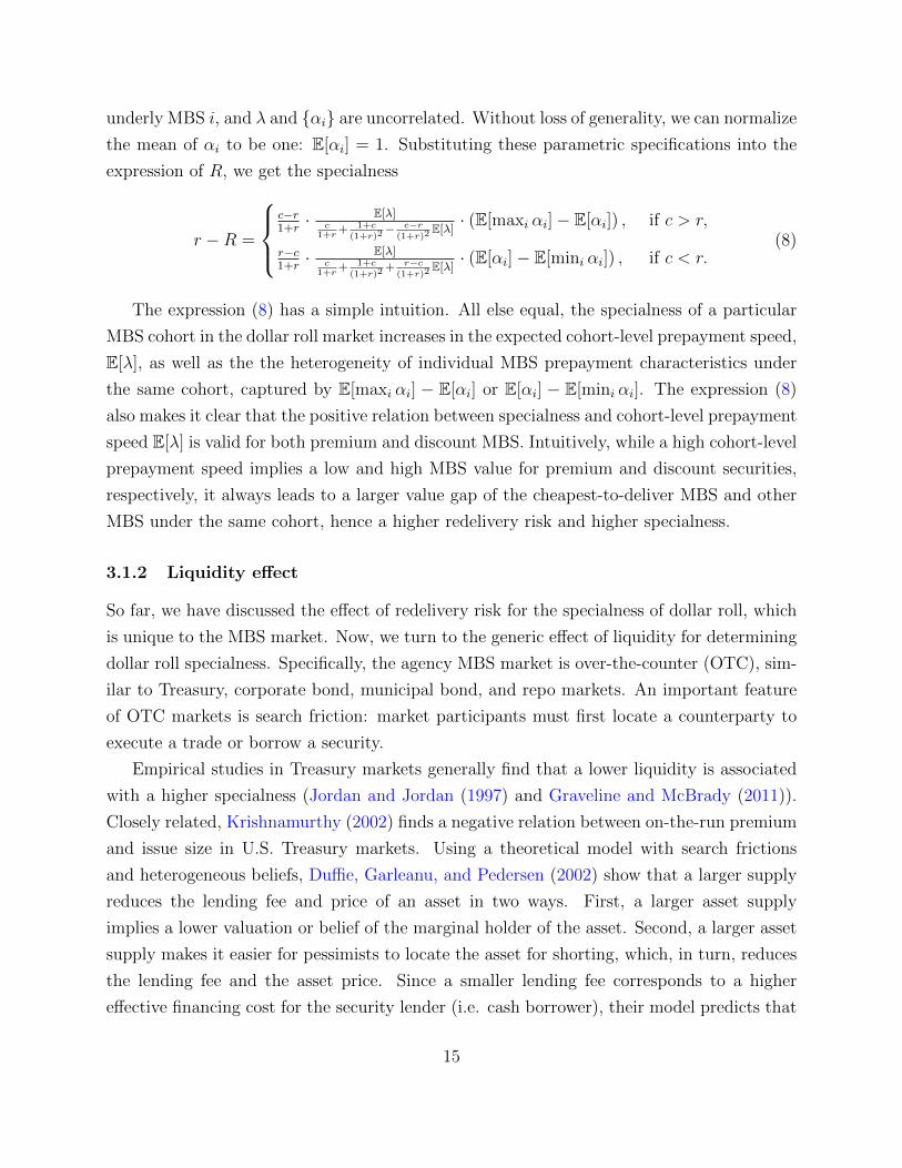
underly MBS i, and λ and {αi} are uncorrelated. Without loss of generality, we can normalize

the mean of αi to be one: E[αi] = 1. Substituting these parametric specifications into the

expression of R, we get the specialness

r −R =

c−r1+r· E[λ]

c1+r

+ 1+c

(1+r)2− c−r

(1+r)2E[λ] · (E[maxi αi]− E[αi]) , if c > r,

r−c1+r· E[λ]

c1+r

+ 1+c

(1+r)2+ r−c

(1+r)2E[λ] · (E[αi]− E[mini αi]) , if c < r.

(8)

The expression (8) has a simple intuition. All else equal, the specialness of a particular

MBS cohort in the dollar roll market increases in the expected cohort-level prepayment speed,

E[λ], as well as the the heterogeneity of individual MBS prepayment characteristics under

the same cohort, captured by E[maxi αi] − E[αi] or E[αi] − E[mini αi]. The expression (8)

also makes it clear that the positive relation between specialness and cohort-level prepayment

speed E[λ] is valid for both premium and discount MBS. Intuitively, while a high cohort-level

prepayment speed implies a low and high MBS value for premium and discount securities,

respectively, it always leads to a larger value gap of the cheapest-to-deliver MBS and other

MBS under the same cohort, hence a higher redelivery risk and higher specialness.

3.1.2 Liquidity effect

So far, we have discussed the effect of redelivery risk for the specialness of dollar roll, which

is unique to the MBS market. Now, we turn to the generic effect of liquidity for determining

dollar roll specialness. Specifically, the agency MBS market is over-the-counter (OTC), sim-

ilar to Treasury, corporate bond, municipal bond, and repo markets. An important feature

of OTC markets is search friction: market participants must first locate a counterparty to

execute a trade or borrow a security.

Empirical studies in Treasury markets generally find that a lower liquidity is associated

with a higher specialness (Jordan and Jordan (1997) and Graveline and McBrady (2011)).

Closely related, Krishnamurthy (2002) finds a negative relation between on-the-run premium

and issue size in U.S. Treasury markets. Using a theoretical model with search frictions

and heterogeneous beliefs, Duffie, Garleanu, and Pedersen (2002) show that a larger supply

reduces the lending fee and price of an asset in two ways. First, a larger asset supply

implies a lower valuation or belief of the marginal holder of the asset. Second, a larger asset

supply makes it easier for pessimists to locate the asset for shorting, which, in turn, reduces

the lending fee and the asset price. Since a smaller lending fee corresponds to a higher

effective financing cost for the security lender (i.e. cash borrower), their model predicts that

15

specialness is lower if the asset supply is larger.14

In a similar vein, dollar roll specialness should increase in the illiquidity of the agency

MBS market. Specifically, if MBS supply for dollar roll trading is scarce, it is more costly for

roll buyers to locate these MBS due to search frictions. Roll sellers who hold the scarce MBS

will command a compensation and hence low borrowing rate for giving up these MBS to roll

buyers in the funding period. Note that the illiquidity here is due to the scarcity of CTD

MBS collateral that are specific to dollar roll trading, rather than any agency MBS collateral

qualified for GC repo trading. Consequently, this illiquidity will affect the dollar roll more

than the repo, leading to high specialness. In sum, we expect that dollar roll specialness is

negatively associated with MBS liquidity.

3.2 Relation between dollar roll specialness and MBS returns

As we have discussed, a dollar roll can become more special for two reasons: a higher adverse

selection associated with redelivery risk or a lower liquidity. For both channels, dollar roll

specialness is negatively related to the expected MBS returns. The generic rationale is

that a high specialness of an MBS gives its holders a “convenience yield” in the financing

market, and these holders are willing to accept a lower expected return in the cash market,

as illustrated in Duffie (1996) and Duffie, Garleanu, and Pedersen (2002).

A unique feature of dollar roll specialness is that the adverse selection channel narrows

down the effective supply and liquidity of the MBS cohort to the cheapest-to-deliver pool of

MBS, as investors rationally redeliver the cheapest CUSIPs in the future-month leg of dollar

roll contracts. By definition, this effective supply of an MBS cohort, comprising of cheapest-

to-deliver MBS CUSIPs, is smaller than the supply of all CUSIPs in the MBS cohort. Even

if the total supply of MBS in a cohort stays constant (which implies zero specialness due to

the general liquidity channel), a higher adverse selection can shrink the effective supply of

the MBS cohort and make it on special. This endogenous feedback between adverse selection

and supply is unique to dollar roll and different from the total supply channel that is also

present in repo market, though both induce a negative relation between the specialness and

expected MBS return as discussed above.

14Not all theories of OTC markets generate unambiguous predictions about the relation between assetsupply and specialness. For example, Vayanos and Weill (2008) characterize the endogenous concentrationof liquidity and trading activity in one asset even if there is another identical asset. They show that, if thesupply of Asset 1 exceeds that of Asset 2 by a sufficient amount, short sellers concentrate on Asset 1. Inthis equilibrium, a decrease in the supply of Asset 1 can lead to a higher or a lower specialness of Asset 1.This ambiguous prediction comes from the interaction between scarcity in the repo market and scarcity inthe spot market.

16

4 Data

Our empirical analysis employs two main proprietary data sets. The first comprises ob-

servations of dollar roll implied financing rates (IFRs), option-adjusted spreads (OAS), and

(realized) single monthly mortality rates (SMM) for FNMA 30-year (generic) TBA contracts

for the next two delivery months and with twelve coupon rates ranging from 3% to 8.5%

from January 2000 to July 2013. These variables are furnished by J.P. Morgan. The dollar

roll financing rates are computed based on expected prepayment rate from their proprietary

prepayment model that is recalibrated to historical data every month. The option-adjusted

spread is a spread added to the term structure of interest rates such that the present value

of an MBS’ expected cash flows, after adjusting for the value of homeowners’ prepayment

options conditional on the interest rate path, equals the price of the security.15 Intuitively,

the OAS measures the expected return an investor earns, relative to certain benchmark in-

terest rates, by buying the MBS and hedging out the expected prepayments. The (realized)

single monthly mortality rate equals the realized prepayment amount as a percentage of the

previous month’s outstanding balance minus this month’s scheduled principal payment. The

SMM is a widely used measure of monthly prepayment rate (see Hayre (2001)).16

The IFR, OAS, and SMM data are available at the daily frequency. We construct monthly

series to (1) align with other important variables that are only available at the monthly fre-

quency, such as the supply of the CTD cohort and MBS characteristics; and (2) reduce noises

associated with microstructure effects. Specifically, our monthly series are constructed as

averages from seven trading days to three trading days (both inclusive) before the settle-

ment date of each month.17 As shown by Gao, Schultz, and Song (2015), dollar roll trading

15 Specifically, let rt, t = 1, · · · , T be the path of one-period interest rate with a realization ofrjt, t = 1, · · · , T under the economy state j = 1, · · · , N . With a prepayment model that specifies the pre-payment behavior of the homeowner conditional on the realized interest rate path under state j, the cashflow path from the MBS Cjt, t = 1, · · · , T can be calculated. Then the OAS is defined such that

VMBS =

N∑j=1

pj

[T∑

t=1

Cjt

(1 + rj1 +OAS)× · · · (1 + rjt +OAS)

],

where pj is the probability of state j. That is, the OAS is the yield spread to the interest rate rt required toset the present value of the MBS expected cash flows based on the prepayment forecast equal to the marketprices of this MBS.

16Our results (presented later) do not hinge on the J.P. Morgan data set. We obtained similar main resultsusing the IFR and OAS data from Barclays, confirming the robustness of our results to different dealers’prepayment models. Moreover, although dealers update their prepayment models periodically, our IFR andOAS series are computed under the same prepayment model of J.P. Morgan over our sample period, so thatthe data contain no artificial discontinuities due to potential updates of the prepayment model.

17We also conducted our main empirical analysis using the end-of-month series, the first-Friday series, and

17

volumes are concentrated in this period of the month. Moreover, close to the settlement

date of the front-month leg, the roll buyer faces little uncertainty regarding the value of the

MBS collateral that he receives, because investors (both sellers and buyers of the dollar roll)

generally have a good idea about what CUSIPs constitute the cheapest-to-deliver cohort a

few days before the settlement date. Overall, our first main data set is an unbalanced panel,

with the common last observations in July 2013 but varying initial observations between

January 2000 and August 2010.

Our second main proprietary data set contains the monthly characteristics of all available

TBA-eligible FNMA 30-year MBS CUSIPs. For each MBS CUSIP, this data set reports the

average FICO score, average loan-to-value ratio (LTV), remaining principal balance, the

percentage of the refinance loans, weighted average coupon rate (WAC), weighted average

maturity (WAM), production year, and issuance amount. These data are obtained from

eMBS and are available from July 2005 through July 2013.

Panel A of Table 1 provides summary statistics of IFRs, in basis points. We observe

that the time series mean of IFRs increases with the coupon rate, with negative values for

coupon rates from 3% to 4%. For all coupon levels, the time-series minimum IFRs are

negative, reaching as low as −13% for the 7% coupon cohort. We compute two versions of

dollar roll specialness, DSPGC and DSPLIBOR, using the 1-month general collateral (GC)

repo rate of agency MBS and the 1-month LIBOR as benchmark prevailing interest rates,

respectively.18 We obtain the ICAP GC repo rate of MBS from Bloomberg and LIBOR

from Datastream. Panels B and C of Table 1 report summary statistics of DSPGC and

DSPLIBOR, respectively. Overall, the average specialness has an approximate range between

20 and 100 basis points if positive, and the time-series mean of dollar roll specialness generally

decreases with the coupon rate (which is due to the “burnout effect” that we discuss in the

last part of Section 5). Specialness for coupon rates from 7.5% to 8.5% is negative on average.

Unsurprisingly, DSPGC is lower than DSPLIBOR because the GC repo rate of MBS is usually

below the 1-month LIBOR. Panel D of Table 1 presents the fraction of time when dollar roll

is “on special.” We observe that dollar roll specialness is positive in over 65% of the sample

period for TBA contracts with coupon rates less than 7%. MBS with very low coupons, e.g.,

from 3% to 4%, and the “current coupon” MBS (with a coupon rate that makes its price

equal to par) are almost always special.

Figure 3 shows the time series behavior of the dollar roll specialness of FNMA 30-year

the calendar-month-average series. The results are similar.18We also use the GCF repo rates of agency MBS, which are only available from May 2005, and obtain

similar results.

18

Table

1:

Sum

mary

Sta

tist

ics

of

Doll

ar

Roll

Fin

anci

ng

Rate

sand

Sp

eci

aln

ess

Cou

pon

(%)

33.

54

4.5

55.5

66.5

77.5

88.5

CC

A:

Doll

ar

Roll

Fin

an

cin

gR

ate

sM

ean

-78.

6-7

2.7

-12.

4152

131.5

221.1

241.2

233.5

227.6

349.1

385.8

464.3

222

Std

77.1

93.4

40.6

219.8

224.1

247.2

238.6

254.2

280.7

225.7

206.4

155.5

249.4

Min

-260

.6-5

11.6

-204

.6-1

97.4

-230.2

-216

-143.3

-670.3

-1363.1

-1098.5

-406.3

58

-610.8

Max

20.6

1843

.6539.7

544.8

683.2

676.2

668.3

659.7

675.6

865

934.8

651.7

B:

DS

PG

C

Mea

n10

4.8

101.

340

.936

53.7

33.3

19.6

27.3

33.3

-88.2

-125

-203.4

38.9

Std

76.3

100.

946

.362.6

71.5

63.6

60.3

85

135.2

176.4

202.2

226.6

72.5

Min

6.2

2.6

-15.

6-1

87.6

-192.1

-202.7

-216.1

-217.8

-252.7

-516.5

-648.2

-909.1

-198.4

Max

291.

460

4.7

288.

8299.3

257.2

230.8

187.6

691.8

1384.7

1120

427.9

218.2

641.8

C:

DS

PL

IBO

R

Mea

n10

1.7

99.1

39.

741

58.7

39.6

26

33.8

39.7

-81.8

-118.5

-197

45.3

Std

77.9

97.5

47.1

58.2

66.4

60.7

57.8

82.6

134

178.8

203.5

229.1

69.6

Min

5.7

2.2

-22.

9-1

68.4

-173

-183.6

-214

-198.7

-254.7

-521.3

-652.9

-911

-179.3

Max

286.

856

3.1

301.

6303.1

253.9

235.3

191.7

693.2

1386

1121.4

429.2

225.6

635.4

D:

Rati

oof

“O

nS

pec

ial”

Beg

in08

/201

012

/200

812

/200

805/2003

08/2002

11/1998

07/1998

07/1998

07/1998

07/1998

07/1998

07/1998

07/1998

En

d07

/201

307

/201

307

/201

307/2013

07/2013

07/2013

07/2013

07/2013

07/2013

07/2013

07/2013

07/2013

07/2013

No.

3656

56123

132

177

181

181

181

181

181

181

181

“Sp

ecia

l”%

-GC

100%

100%

96%

80%

82%

72%

64%

69%

64%

31%

36%

20%

88%

-LIB

OR

100%

100%

95%

88%

90%

81%

71%

75%

70%

35%

36%

22%

94%

Not

e:T

his

tab

lep

rovid

essu

mm

ary

stat

isti

csof

the

fin

an

cin

gra

tes,

spec

ialn

ess

rela

tive

tob

oth

the

GC

rep

ora

tean

dL

IBO

R,

an

dth

era

tio

ofd

olla

rro

llb

ein

gon

spec

ial

inth

eti

me

seri

es,

acr

oss

cou

pon

rate

s.T

he

valu

esof

fin

an

cin

gra

tes

an

dsp

ecia

lnes

sare

den

ote

din

basi

sp

oin

ts.

Th

ela

stco

lum

n“C

C”

refe

rsto

“cu

rren

t-co

up

onM

BS

”,

wh

ich

isth

eM

BS

wit

ha

cou

pon

rate

that

makes

its

pri

ceeq

ual

top

ar.

Th

eov

erall

sam

ple

per

iod

isJan

uar

y20

00to

Ju

ly20

13,

wit

hva

riou

sst

art

ing

date

sth

at

dep

end

on

cou

pon

rate

s.

19

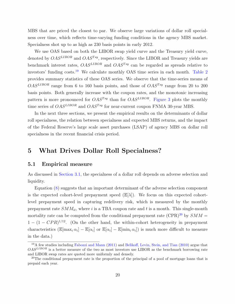
MBS that are priced the closest to par. We observe large variations of dollar roll special-

ness over time, which reflects time-varying funding conditions in the agency MBS market.

Specialness shot up to as high as 230 basis points in early 2012.

We use OAS based on both the LIBOR swap yield curve and the Treasury yield curve,

denoted by OASLIBOR and OASTsy, respectively. Since the LIBOR and Treasury yields are

benchmark interest rates, OASLIBOR and OASTsy can be regarded as spreads relative to

investors’ funding costs.19 We calculate monthly OAS time series in each month. Table 2

provides summary statistics of these OAS series. We observe that the time-series means of

OASLIBOR range from 6 to 160 basis points, and those of OASTsy range from 20 to 200

basis points. Both generally increase with the coupon rates, and the monotonic increasing

pattern is more pronounced for OASTsy than for OASLIBOR. Figure 3 plots the monthly

time series of OASLIBOR and OASTsy for near-current coupon FNMA 30-year MBS.

In the next three sections, we present the empirical results on the determinants of dollar

roll specialness, the relation between specialness and expected MBS returns, and the impact

of the Federal Reserve’s large scale asset purchases (LSAP) of agency MBS on dollar roll

specialness in the recent financial crisis period.

5 What Drives Dollar Roll Specialness?

5.1 Empirical measure

As discussed in Section 3.1, the specialness of a dollar roll depends on adverse selection and

liquidity.

Equation (8) suggests that an important determinant of the adverse selection component

is the expected cohort-level prepayment speed (E[λ]). We focus on this expected cohort-

level prepayment speed in capturing redelivery risk, which is measured by the monthly

prepayment rate SMMit, where i is a TBA coupon rate and t is a month. This single-month

mortality rate can be computed from the conditional prepayment rate (CPR)20 by SMM =

1 − (1 − CPR)1/12. (On the other hand, the within-cohort heterogeneity in prepayment

characteristics (E[maxi αi] − E[αi] or E[αi] − E[mini αi]) is much more difficult to measure

in the data.)

19A few studies including Fabozzi and Mann (2011) and Belikoff, Levin, Stein, and Tian (2010) argue thatOASLIBOR is a better measure of the two as most investors use LIBOR as the benchmark borrowing rateand LIBOR swap rates are quoted more uniformly and densely.

20The conditional prepayment rate is the proportion of the principal of a pool of mortgage loans that isprepaid each year.

20

Table

2:

Sum

mary

Sta

tist

ics

of

Opti

on-A

dju

sted

Spre

ads

OASLIBOR

Cou

pon

(%)

33.

54

4.5

55.

56

6.5

77.

58

8.5

CC

Mea

n32

.02

19.

9815

.313

.55

5.99

12.3

615

.65

21.1

32.8

991

.85

113.

3116

2.63

11.6

8

Std

27.

0819.9

912

.97

21.3

927

.35

25.6

430

.63

36.7

447

.05

120.

815

2.41

176.

4117

.52

Min

-19.6

9-3

1.1

9-1

1.2

7-3

7.72

-85.

89-6

3.76

-71.

33-3

5.89

-45.

05-4

1.15

-82.

55-5

5.61

-15.

64

Max

82.9

375.

8959.5

281

.94

75.9

510

9.97

150.

0919

1.4

220.

9637

7.64

424.

949

3.37

68.6

9

OASTsy

Mea

n28

.99

22.

9819.3

543

.91

37.7

939

.28

43.5

550

.767

.412

8.56

150.

9420

3.07

43.4

4

Std

27.

4824.4

116

.67

33.8

339

.95

35.6

838

.64

41.7

549

.42

110.

1613

9.88

163.

6827

.1

Min

-28.4

1-3

5.4

2-1

5.6

6-3

7.77

-82.

54-5

8.89

-67.

85-2

3.4

-12.

9-5

.63

-43.

44-1

7.08

-21.

22

Max

75.3

3104

.581.8

415

8.92

150.

8915

1.4

171.

4320

4.48

253.

8638

9.99

438.

0150

7.21

152.

36

Not

e:T

his

tab

lep

rovid

essu

mm

ary

stat

isti

csof

month

lyse

ries

ofOASLIBOR

an

dOASTsy

acr

oss

cou

pon

rate

s.T

he

OA

Sva

lues

are

den

ote

d

inb

asis

poi

nts

.T

he

last

colu

mn

“CC

”re

fers

to“cu

rren

t-co

up

on

MB

S”,

wh

ich

isth

eM

BS

wit

ha

cou

pon

rate

that

make

sit

spri

ceeq

ual

to

par

.T

he

over

all

sam

ple

per

iod

isJan

uar

y20

00to

Ju

ly2013,

wit

hva

riou

sst

art

ing

date

sth

at

dep

end

on

cou

pon

rate

s.

21

Figure 3: Specialness and OAS of Near-Current Coupon Dollar Roll

DateJan-02 Jan-04 Jan-06 Jan-08 Jan-10 Jan-12

Bas

is P

oint

s

-200

-150

-100

-50

0

50

100

150

200

250Specialness of Near-Current Coupon Dollar Roll

Dollar Roll Specialness-LIBORDollar Roll Specialness-GC

Jan−05 Jan−10−40

−20

0

20

40

60

80

100

120

140

160

Date

Bas

is P

oint

s

Option Adjusted Spreads of Near−Current Coupon MBS

LIBOR−OASTsy−OAS

Note: This figure plots monthly time series of the specialness, as well as OASLIBOR and OASTsy, of FNMA

30-year MBS that are priced the closest to par, from January 2000 to July 2013. The dollar roll specialness

is computed both relative to the 1-month GC repo rate of agency MBS and to the 1-month LIBOR.

22

To capture the liquidity effect, one reasonable proxy is the available supply of MBS to

settle dollar roll trades.21 Importantly, the supply measure should be about the CTD cohort,

i.e., those CUSIPs most advantageous to deliver into TBA contracts by investors, rather than

the total outstanding balance of all MBS. To the best of our knowledge, there are no readily

available data that tell whether an MBS CUSIP is part of the CTD cohort. Thus, we

construct the set of CTD cohort based on criteria similar to those in Himmelberg, Young,

Shan, and Henson (2013), using data on MBS characteristics. Specifically, for each TBA

coupon in each month, we eliminate MBS CUSIPs that have at least one of the following

characteristics: remaining principal balance is less than $150,000, refinance share is greater

than 75%, the average LTV ratio is above 85%, and the average FICO score is below 680.

These characteristics make prepayment less likely; thus, the associated CUSIPs have more

predictable values and are unlikely to become part of the CTD cohort. Adding up the

outstanding amount of the remaining CUSIPs gives us a measure of the (raw) supply of

CTD MBS CUSIPs for each TBA coupon i in each (TBA settlement) month t, denoted

SupplyCTDit .22

We further adjust SupplyCTDit by the demand for the CTD cohort to get a measure of

the net CTD supply. As discussed in Section 2, one important source of TBA demand is

the amount of CMO deals that MBS dealers need to cover. We obtain the monthly agency

CMO volume from Bloomberg and subtract it from SupplyCTDit to get a net-supply measure,

denoted as NSupplyCTDit .23

Table 3 reports the summary statistics of SMM and NSupplyCTD across coupons. We

observe that the average prepayment rate in our sample period increases with coupons for

coupon buckets less than 7% and decreases thereafter. The highest monthly prepayment rate

is 3.35% for the 7% coupon MBS. The monthly average of the net supply of CTD MBS is all

above $100 billion for coupons below 6%, and decreases from $20 billion to only $6 million

21Other common measures of liquidity, such as trading volume or bid-ask spread, rely on transaction data,which are unavailable until 2011 when post-trade transparency in MBS was introduced by FINRA.

22The MBS supply variables are available at the end of calendar month, whereas our time index t refers toTBA settlement month. Since the settlement date is usually around the 12th or 13th of a calendar month,SupplyCTD for settlement month t is recorded at the end of calendar month t− 1. The same applies to themeasure NSupplyCTD that we define below.

23Bloomberg provides the monthly agency CMO volume across coupon rates, but no further breakdownacross agencies. To obtain the monthly CMO volume of FNMA across coupons, we multiply the CMOvolume in each coupon bucket by the aggregate ratio of the FNMA CMO (relative to other agencies) foreach month. The computed FNMA CMO volume combines both the 30-year and 15-year collateral. HenceNSupplyCTD

it underestimates the CTD supply, which goes against our results. Therefore, our results areconservative and the regression coefficients NSupplyCTD

it in the following sections should be interpreted asa lower bound. Moreover, results using SupplyCTD

it are similar.

23

Figure 4: Primary and Secondary Mortgage Rates

DateJan-02 Jan-04 Jan-06 Jan-08 Jan-10 Jan-12

Bas

is P

oint

s

200

300

400

500

600

700

800

900Primary and Secondary Mortgage Rate

Primary Mortgage RateCurrent Coupon Rate

Note: This figure plots monthly time series of primary mortgage rates (PMMS) for 30-year fixed-rate mort-

gage loans, from the Freddie Mac primary mortgage market survey, and current-coupon (CC) mortgage rate,

from January 2000 to July 2013.

as the coupon increases from 6.5% to 8.5%. This is unsurprising given that the primary

mortgage rate decreased from 8.5% to 3.5% in our sample period, which shifted the MBS

issuance from high to low coupons (see Figure 4).

5.2 Results

Table 4 reports panel regressions based on the following model:

DSPit =∑t

αtDt +∑i

γiDi + β1 · SMMit + β2 ·NSupplyCTDit + εit, (9)

where DSPit is either DSPGCit or DSPLIBOR

it , and Di and Dt are coupon dummies and

time dummies, respectively. The time dummies control both the time-series persistence in

the data and the effect of certain pure time-series factors, such as interest rate volatility,

financial constraints of financial intermediaries, and house prices, which may also affect

dollar roll specialness (Gabaix, Krishnamurthy, and Vigneron (2007)). We report robust

24

Tab

le3:

Sum

mary

Sta

tist

ics

ofSMM

andNSupplyCTD

SMM

Cou

pon

(%)

33.

54

4.5

55.

56

6.5

77.

58

8.5

Mea

n0.

221

0.7

360.9

081.

308

1.46

11.

768

2.06

92.

632

3.35

43.

318

3.32

32.

694

Std

0.17

10.8

29

1.09

91.

367

1.77

1.61

41.

841

2.37

92.

682

2.97

3.52

2.56

Min

0.00

80.0

42

0.05

0.05

0.05

0.06

70.

101

0.10

10.

168

0.21

10.

017

0.00

8

Max

0.5

85

3.56

33.

444.

416.

426.

048

10.7

0519

.415

20.7

924

.196

35.6

9511

.495

N22

36

5661

123

132

163

163

163

163

163

163

NSuppyCTD

Mea

n-

119.5

89

144

.891

259.

531

113.

016

123.

261

101.

358

19.5

634.

438

0.16

70.

053

0.00

6

Std

-134.

827

63.4

1411

1.99

455

.999

61.1

647

.126

8.14

92.

081

0.09

40.

039

0.00

7

Min

--0

.777

-2.2

49-1

.578

-0.3

810.

001

-0.1

430.

001

0.00

10.

015

-0.0

23-0

.039

Max

-33

0.1

0423

6.39

639

2.25

619

9.75

821

8.28

618

1.56

131

.698

7.96

0.31

10.

113

0.02

N0

34

5556

7070

7070

7068

6868

Not

e:T

his

tab

lep

rovid

essu

mm

ary

stat

isti

csof

month

lyse

ries

ofSMM

an

dNSupply

CTD

acr

oss

cou

pon

rate

s,in

per

centa

ge

poin

tsan

d

bil

lion

sof

U.S

.d

olla

rs,

resp

ecti

vel

y.T

he

over

allsa

mple

per

iod

isJanu

ary

2000

toJu

ly2013,

wit

hva

riou

sst

art

ing

date

sth

at

dep

end

on

cou

pon

rate

s.

25

t-statistics in parentheses that correct for serial correlation in the residuals clustered at the

coupon level.

Table 4: Determinants of Dollar Roll Specialness

DSPGC DSPLIBOR

(1) (2) (3) (4) (5) (6)SMM 7.7540** 21.7924** 7.7540** 21.7924**

(3.1705) (4.3227) (3.1705) (4.3227)

NSupplyCTD -0.1810+ -0.2023* -0.1810+ -0.2023*(-2.1288) (-2.2670) (-2.1288) (-2.2670)

N 719 1,408 719 719 1,408 719

R2 0.8116 0.6346 0.8076 0.8080 0.6299 0.8039Coupon Effect Yes Yes Yes Yes Yes Yes

Time Effect Yes Yes Yes Yes Yes Yes

Note: This table reports panel regressions based on the following model:

DSPit =∑t

αtDt +∑i

γiDi + β1 · SMMit + β2 ·NSupplyCTDit + εit,

where DSPit is either DSPGCit or DSPLIBORit , and Di and Dt are coupon dummies and time

dummies, respectively. Robust t-statistics are reported in parentheses based on clustered standard

errors at the coupon level. Significance levels: ∗∗ for p < 0.01, ∗ for p < 0.05, and + for p < 0.1,

where p is the p-value. The overall sample period is January 2000 to July 2013, with various

starting dates that depend on coupon rates.

Results from Table 4 confirm our hypothesis: a higher prepayment speed, SMM , is

associated with a higher dollar roll specialness, whereas a higher net supply, NSupplyCTD,

is associated with a lower specialness. The economic magnitudes are also large. For example,

reading from column (1), a 2.54 percentage point increase in SMM , which is roughly one

standard deviation of SMM across time and coupon in our sample, increases dollar roll

specialness by about 20 basis points (= 7.7540 × 2.54); and a $99.26 billion increase in the

available supply of the CTD cohort, which is roughly one standard deviation of the balance

of the CTD cohort across time and coupon in our sample, decreases specialness by 18 basis

points (= −0.1810 × 99.26). We also run univariate panel regressions with only one of

SMM and NSupplyCTD on the right-hand side, and the results in columns (2), (3), (5),

and (6) further confirm the significant impact of adverse selection and liquidity on dollar

roll specialness. In all these regressions, using DSPGCit and DSPLIBOR

it yields essentially

identical coefficients.

26

5.3 Alternative measures of prepayment speed

We have shown that a higher cohort-level prepayment speed, SMMit, is associated with a

higher dollar roll specialness. In this subsection we explore two alternative cohort-specific

measures of prepayment speed that are coarser than SMM but come from first principles.

The first alternative measure of cohort-specific prepayment speed is the “burnout effect”

(BO), an interesting feature unique to the mortgage markets. The burnout effect says that

mortgage borrowers who had refinancing opportunities in the past, but chose not to take

them, are less likely to prepay and refinance in the future if mortgage rates fall. The essence of

the burnout effect is that reactions to past refinancing opportunities reveal some unobservable

characteristics (“types”) of borrowers. To see the intuition, consider the following stylized

example. Suppose that mortgage rates have dropped from 5% last year to 4% this year.

Borrowers who benefit most from refinancing at lower rates, and are able to do so, probably

will have already refinanced this year; therefore, their new mortgage loans with lower interest

rates of 4% enter the pool of MBS with coupon rates around 4%. By contrast, borrowers still

paying the 5% mortgage interest this year, despite the lower prevailing rate, signal a high

effective cost of refinancing: the household could have an impaired credit, a low home equity

value, or a small remaining loan balance, among other reasons. All these characteristics

make the households that keep the 5% mortgage loan less likely to refinance in the future

even if rate drops further.

We measure the time-t burnout effect of a TBA cohort with coupon rate CPi as

BOit =t−1∑s=1

(WACis − PMMSs)1(WACis>PMMSs), (10)

where 1{WACis>PMMSs} = 1 if the original coupon rate is higher than the mortgage rate at

time s, and 0 otherwise. The original coupon rate is measured by the weighted average

coupon (WAC) of all MBS in the CTD cohort identified above, weighted by the remaining

balance, while the current mortgage rate is measured by the primary mortgage rate PMMSt

for 30-year fixed-rate mortgage loans from the Freddie Mac primary mortgage market survey,

available at the weekly frequency (we use the first-week series to align with the monthly series

of all other variables). Conditional on WACis > PMMSs, the higher is WACis−PMMSs,

the further the mortgage rate falls below the original coupon rate and hence the more the

MBS is “burned.” Hence, BOit captures the cumulative past exposure up to time t of the

MBS to low mortgage rates (Hall (2000)).

The second alternative measure of cohort-specific prepayment speed is the value of mort-

27

gage borrowers’ prepayment options. At first sight, it may appear that we should use coupon

cohorts that are currently in the money, that is, the prevailing mortgage rates are lower than

the coupon rates. But the burnout effect discussed above suggests that mortgage borrowers

underlying MBS cohorts with in-the-money coupons are, by revealed preference, less rate-

sensitive. To avoid overlapping with the burnout effect measure, we exclude in-the-money

coupon cohorts and focus on out-of-the-money cohorts. Specifically, we measure the current

prepayment incentive of the TBA cohort with coupon CPi at time t by the difference between

the original coupon rate and the current mortgage rate:

PIit = 1{WACit<PMMSt} (WACit − PMMSt) , (11)

where 1{WACit<PMMSt} = 1 if the original coupon rate is lower than the current mortgage

rate, and 0 otherwise. Conditional on WACit < PMMSt, the less negative is WACit −PMMSt, the more valuable is the prepayment option. Put differently, mortgage borrowers’

prepayment options are more valuable if the options are less out of the money. (In the data

there are almost no data points with WACit = PMMSt.)

We emphasize that BO and PI are just two of many possible inputs to prepayment

models whose output is SMM ; hence, we do not have a strong prior that BO or PI alone

would capture prepayment speed as well as SMM does.

Table 5 report results from regression

DSPit =∑t

αtDt +∑i

γiDi + β1 · PIit + β2 ·NSupplyCTDit + εit, (12)

and

DSPit =∑t

αtDt +∑i

γiDi + β1 ·BOit + β2 ·NSupplyCTDit + εit. (13)

We also put PI and BO simultaneously into the same regression. In regressions that include

only one of PI and BO at a time, both channels of prepayments have significant impacts on

the dollar roll specialness. In particular, the higher the current prepayment incentive, the

higher the specialness; the higher the burnout effect, the lower the specialness. If both PI

and BO are included, BO remains significant, whereas PI does not.

28

Table 5: Channels of Prepayment Speed

DSPGC

PI 125.8993+ 122.8218+ 29.0146(2.0353) (1.8602) (0.6881)

BO -1.2686** -1.0674* -1.0278*(-3.7970) (-2.9058) (-2.8186)

NSupplyCTD -0.2707* -0.3150** -0.3273**(-2.5354) (-3.4744) (-3.3469)

N 915 915 719 719 719

R2 0.7693 0.7968 0.8106 0.8226 0.8228Coupon Effect Yes Yes Yes Yes Yes

Time Effect Yes Yes Yes Yes Yes

DSPLIBOR

PI 125.8993+ 122.8218+ 29.0146(2.0353) (1.8602) (0.6881)

BO -1.2686** -1.0674* -1.0278*(-3.7970) (-2.9058) (-2.8186)

NSupplyCTD -0.2707* -0.3150** -0.3273**(-2.5354) (-3.4744) (-3.3469)

N 915 915 719 719 719

R2 0.7654 0.7935 0.8070 0.8193 0.8194Coupon Effect Yes Yes Yes Yes Yes

Time Effect Yes Yes Yes Yes Yes


DSPit =∑t

αtDt +∑i

γiDi + β1 · PIit + β2 ·NSupplyCTDit + εit,

DSPit =∑t

αtDt +∑i

γiDi + β1 ·BOit + β2 ·NSupplyCTDit + εit,

and a regression that includes both PI and BO on the right-hand side. Here, DSPit is either

DSPGCit or DSPLIBORit , and Di and Dt are coupon dummies and time dummies, respectively.

Robust t-statistics are reported in parentheses based on clustered standard errors at the coupon

level. Significance levels: ∗∗ for p < 0.01, ∗ for p < 0.05, and + for p < 0.1, where p is the p-value.

The overall sample period is January 2000 to July 2013, with various starting dates that depend

on coupon rates.

29

6 Dollar Roll Specialness and Expected MBS Returns

In this section, we study the relation between doll roll specialness and expected MBS returns.

We find a negative relation, as hypothesized in Section 3.2.

A commonly used measure of expected MBS returns is the option-adjusted spread (OAS)

(see Gabaix, Krishnamurthy, and Vigneron (2007)). As we discussed in the data section,

the OAS is effectively a model-implied yield spread of an MBS relative to a benchmark

interest-rate term structure, after adjusting for the value of homeowners’ expected prepay-

ment options.

Figure 5 plots the time-series averages of OASLIBOR and OASTsy, together with those

of DSPGC across coupon rates. A pronounced negative relation emerges. As coupon rate

increases, specialness goes down, but OAS goes up.

Figure 5: Dollar Roll Specialness and OAS across Coupons

Bas

is P

oint

s

-250

-200

-150

-100

-50

0

50

100

150

200

250

3% 3.5% 4% 4.5% 5% 5.5% 6% 6.5% 7% 7.5% 8% 8.5%

Specialness vs OAS

Roll Specialness-GC RepoLIBOR OASTsy OAS

Note: This figure plots time series averages of OASLIBOR and OASTsy together with those of

DSPGC across coupon rates. The overall sample period is January 2000 to July 2013, with various


To quantify the relation between dollar roll specialness and OAS across coupon rates and

time, the first two columns of both Panels A and B of Table 6 report panel regressions on

30

the following model:

OASit =∑t

αtDt +∑i

γiDi + β · 1(DSPit > 0) + εit, (14)

where 1(DSPit > 0) is the specialness indicator function, taking on the value of 1 if an MBS

cohort with coupon CPi is on special in period t and 0 otherwise, OASit is either OASLIBOR

or OASTsy, and Di and Dt are coupon dummies and time dummies, respectively. Robust

t-statistics are reported in parentheses that correct for serial correlation in the residuals

clustered at the coupon level. We observe that an MBS cohort on special has a significant

negative premium relative to an otherwise identical MBS cohort. In particular, the negative

premium is about 50 and 60 basis points using OASTsy and OASLIBOR, respectively, for

both DSPGCit and DSPLIBOR

it .

Furthermore, the last two columns of both Panels A and B of Table 6 report panel

regressions using the magnitude of dollar roll specialness:

OASit =∑t

αtDt +∑i

γiDi + β ·DSPit + εit, (15)


it . We observe highly significant impact of dollar

roll specialness on OAS, regardless of which interest benchmark interest rates are used to

compute specialness, which OAS measure is used, and whether coupon and time effects are

included. The coefficient estimates are remarkably stable, ranging from −0.50 to −0.41.24

Regressing the OAS on dollar roll specialness may suffer from an endogeneity problem

as both are outputs from a prepayment model with the same inputs. To investigate the

robustness of our results, we use another proprietary data set provided by J.P. Morgan

that consists of monthly returns on FNMA 30-year TBA contracts from February 2000 to

July 2013. The return series are calculated for a strategy of going long a one-month TBA,

investing the TBA price in a riskless margin account, and then rolling the portfolio over

every month on the monthly TBA settlement date. (Carlin, Longstaff, and Matoba (2014)

employ a data set of return series with the same strategy.) By design, these return series do

not depend on any model or assumption about mortgage prepayment rates or interest rate

paths. We label this returns series the “return on mortgages,” or ROM . Regressing ROM

on dollar roll specialness is free of the endogeneity problem of regressing OAS on specialness.

24We also run the first-difference regression and still find highly significant and negative relation betweendollar roll specialness and OAS.

31

Table 6: Regression of OAS on Specialness

A: OASLIBOR B: OASTsy

1(DSPGC> 0) -60.79** -54.62**

(-4.13) (-3.95)1(DSP

LIBOR> 0) -59.90** -53.36**

(-4.15) (-3.94)DSPGC -0.45** -0.41**

(-7.06) (-6.39)DSPLIBOR -0.45** -0.41**

(-7.11) (-6.44)

N 1,666 1,666 1,666 1,666 1,666 1,666 1,666 1,666R2 0.61 0.61 0.80 0.80 0.61 0.61 0.78 0.78

Coupon Effect Yes Yes Yes Yes Yes Yes Yes YesTime Effect Yes Yes Yes Yes Yes Yes Yes Yes

Note: The first two columns of each panel report panel regressions based on

OASit =∑t

αtDt +∑i

γiDi + β · 1(DSPit > 0) + εit,

while the last two columns of each panel report panel regressions based on

OASit =∑t

αtDt +∑i

γiDi + β ·DSPit + εit,

where 1(DSPit > 0) is either 1(DSPGCit > 0) or 1(DSPLIBORit > 0), DSPit is either DSPGCit or

DSPLIBORit , OASit is either OASLIBOR or OASTsy, and Di and Dt are coupon dummies and time



where p is the p-value. The overall sample period is July 2000 to July 2013, with various starting

dates that depend on coupon rates.

Columns (1) and (2) of Table 7 report panel regressions based on the model

ROMit =∑t

αtDt +∑i

γiDi + β ·DSPit + εit, (16)

whereas columns (3) and (4) report panel regressions based on the model

ROMit =∑t

αtDt +∑i

γiDi + β ·∆DSPit + εit, (17)

32

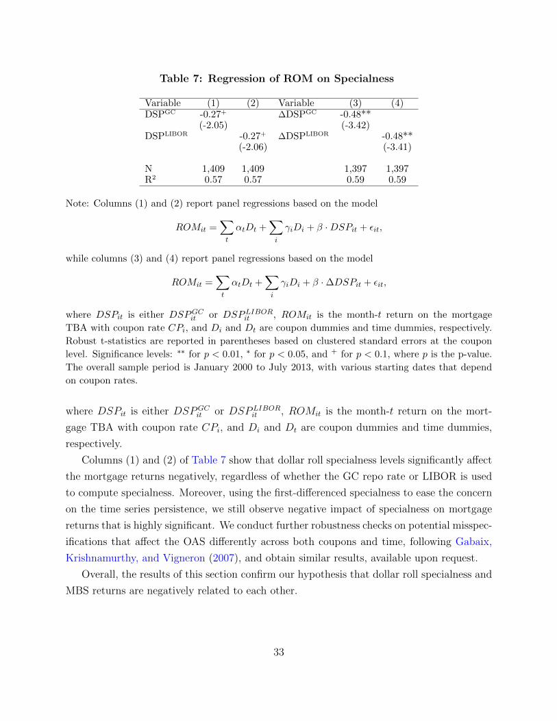
Table 7: Regression of ROM on Specialness

Variable (1) (2) Variable (3) (4)DSPGC -0.27+ ∆DSPGC -0.48**

(-2.05) (-3.42)DSPLIBOR -0.27+ ∆DSPLIBOR -0.48**

(-2.06) (-3.41)

N 1,409 1,409 1,397 1,397R2 0.57 0.57 0.59 0.59

Note: Columns (1) and (2) report panel regressions based on the model

ROMit =∑t

αtDt +∑i

γiDi + β ·DSPit + εit,

while columns (3) and (4) report panel regressions based on the model

ROMit =∑t

αtDt +∑i

γiDi + β ·∆DSPit + εit,

where DSPit is either DSPGCit or DSPLIBORit , ROMit is the month-t return on the mortgage

TBA with coupon rate CPi, and Di and Dt are coupon dummies and time dummies, respectively.

Robust t-statistics are reported in parentheses based on clustered standard errors at the coupon

level. Significance levels: ∗∗ for p < 0.01, ∗ for p < 0.05, and + for p < 0.1, where p is the p-value.

The overall sample period is January 2000 to July 2013, with various starting dates that depend

on coupon rates.


it , ROMit is the month-t return on the mort-

gage TBA with coupon rate CPi, and Di and Dt are coupon dummies and time dummies,

respectively.

Columns (1) and (2) of Table 7 show that dollar roll specialness levels significantly affect

the mortgage returns negatively, regardless of whether the GC repo rate or LIBOR is used

to compute specialness. Moreover, using the first-differenced specialness to ease the concern

on the time series persistence, we still observe negative impact of specialness on mortgage

returns that is highly significant. We conduct further robustness checks on potential misspec-

ifications that affect the OAS differently across both coupons and time, following Gabaix,

Krishnamurthy, and Vigneron (2007), and obtain similar results, available upon request.

Overall, the results of this section confirm our hypothesis that dollar roll specialness and

MBS returns are negatively related to each other.

33

7 The Impact of LSAP on Dollar Roll Specialness

In response to the recent financial crisis, the Federal Reserve introduced a sequence of large-

scale asset purchase (LSAP) programs of agency MBS, as well as of Treasury securities, for

the purpose of “credit easing” (Bernanke (2009)). The first LSAP program of agency MBS

was announced in November 2008. The MBS purchases did not start until January 2009, and

were finished in March 2010, with a total size of around $1.25 trillion as planed. Then, in

September 2011, the Federal Reserve decided to reinvest principal payments from its agency

MBS holdings into agency MBS markets, rather than into long-term Treasury securities as

it has been doing since August 2010. Finally, in September 2012, another LSAP program

of agency MBS began when the Federal Reserve announced that it will purchase additional

agency MBS at a pace of $40 billion per month until the labor market and financial market

conditions improve substantially. Together with the reinvestments from its agency MBS

holdings, the Federal Reserve has been purchasing around $45–55 billion of agency MBS

per month from September 2012 till the end of our sample period July 2013.25 The great

majority of these purchases are newly issued 15- and 30-year agency MBS with production

coupons, which vary over time with the primary mortgage rate. The Fed’s MBS purchases

are executed exclusively in the TBA market.

Given the large size of the Federal Reserve’s agency MBS purchases, one natural question

is whether LSAP “disrupts” the functioning of the agency MBS market. In this section, we

investigate this question by studying whether the Federal Reserve’s purchases affected dollar

roll specialness. We obtain the Federal Reserve’s transactions data of the FNMA 30-year

MBS with different coupon rates from the website of the Federal Reserve Bank of New York.

We also obtain the monthly new issuance (ISUit) as well as the current outstanding balance

(CBit) of FNMA 30-year MBS pools across coupon rates, both from the eMBS, to normalize

the LSAP size.

Figure 6 plots the aggregate LSAP purchase amount of FNMA 30-year MBS across

coupon rates, along with amounts of outstanding balance, from January 2009 to July 2013.26

We observe that total LSAP size, outstanding balance, and LSAP size as a fraction of

25On December 18, 2013, the Fed began “tapering” its asset purchases, with a reduction of $5 billion permonth on MBS purchases. The scheduled MBS purchases ended in October 2014, although the Fed continuesreinvesting in MBS the principal and coupon payments from its existing holdings.

26It is worth pointing out that the total purchase size does not take into account the principal payout,and accordingly the outstanding balance in Figure 6 is computed as the sum of the outstanding balanceas of December 2008, the last month before the start of LSAP purchases, and the cumulative new issuancebetween March 2009 and July 2013. Thus, the true outstanding balance may be mildly smaller than thatshown.

34

Figure 6: Size of LSAP

0

100

200

300

400

500

600

700

Bill

ion

Dol

lars

Total LSAP Size vs Outstanding Balance

3% 3.5% 4% 4.5% 5% 5.5% 6% 6.5%

Total LSAP Size (left)Outstanding Balance (left)

0

0.1

0.2

0.3

0.4

0.5

0.6

0.7

0.8

0.9

1

Total LSAP Size/Outstanding Balance (right)

Note: This figure plots cumulative size of LSAP vs outstanding balance of MBS. The sample is from January

2009 to July 2013.

outstanding balance are all hump-shaped in coupon rate. The Fed has absorbed more than

50% of all outstanding balance of FNMA 30-year MBS with coupon rates from 3% to 5.5%.

The fraction is over 90% for the 5% and 5.5% coupon cohorts.

We consider five measures for the Federal Reserve’s MBS purchases LSAPit: the purchase

size QLSAPit (in billions of US dollars), the purchase size as a ratio of the month-t aggregate

issuance QLSAPit /ISUit, the indicator 1(Flowit) of purchases in month t for coupon CPi, the

cumulative purchase size as a ratio of the month-t outstanding balance QCumulativeit /CBit, and

the indicator 1(Stockit) for the existence of MBS with coupon CPi in the Federal Reserve’s

holdings at month t. To align with the monthly specialness measures calculated over the

active trading period before the settlement date of each month, we compute QLSAPit as the

aggregate purchase amount in this coupon from the day after settlement of month t − 1

to two days before the settlement of month t. All other LSAP variables are constructed

similarly.

35

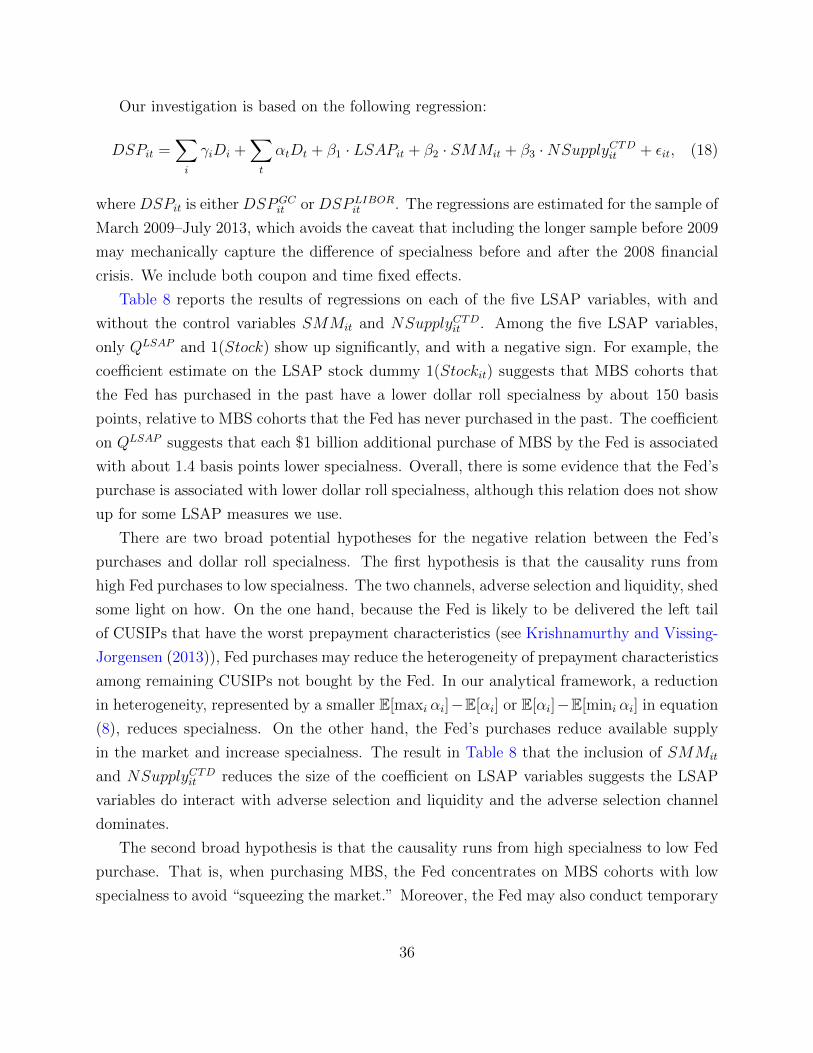
Our investigation is based on the following regression:

DSPit =∑i

γiDi +∑t

αtDt + β1 · LSAPit + β2 · SMMit + β3 ·NSupplyCTDit + εit, (18)


it . The regressions are estimated for the sample of

March 2009–July 2013, which avoids the caveat that including the longer sample before 2009

may mechanically capture the difference of specialness before and after the 2008 financial

crisis. We include both coupon and time fixed effects.

Table 8 reports the results of regressions on each of the five LSAP variables, with and

without the control variables SMMit and NSupplyCTDit . Among the five LSAP variables,

only QLSAP and 1(Stock) show up significantly, and with a negative sign. For example, the

coefficient estimate on the LSAP stock dummy 1(Stockit) suggests that MBS cohorts that

the Fed has purchased in the past have a lower dollar roll specialness by about 150 basis

points, relative to MBS cohorts that the Fed has never purchased in the past. The coefficient

on QLSAP suggests that each $1 billion additional purchase of MBS by the Fed is associated

with about 1.4 basis points lower specialness. Overall, there is some evidence that the Fed’s

purchase is associated with lower dollar roll specialness, although this relation does not show

up for some LSAP measures we use.

There are two broad potential hypotheses for the negative relation between the Fed’s

purchases and dollar roll specialness. The first hypothesis is that the causality runs from

high Fed purchases to low specialness. The two channels, adverse selection and liquidity, shed

some light on how. On the one hand, because the Fed is likely to be delivered the left tail

of CUSIPs that have the worst prepayment characteristics (see Krishnamurthy and Vissing-

Jorgensen (2013)), Fed purchases may reduce the heterogeneity of prepayment characteristics

among remaining CUSIPs not bought by the Fed. In our analytical framework, a reduction

in heterogeneity, represented by a smaller E[maxi αi]−E[αi] or E[αi]−E[mini αi] in equation

(8), reduces specialness. On the other hand, the Fed’s purchases reduce available supply

in the market and increase specialness. The result in Table 8 that the inclusion of SMMit

and NSupplyCTDit reduces the size of the coefficient on LSAP variables suggests the LSAP

variables do interact with adverse selection and liquidity and the adverse selection channel

dominates.

The second broad hypothesis is that the causality runs from high specialness to low Fed

purchase. That is, when purchasing MBS, the Fed concentrates on MBS cohorts with low

specialness to avoid “squeezing the market.” Moreover, the Fed may also conduct temporary

36

market operations by buying and selling dollar roll contracts to alleviate supply shortage.

This hypothesis is in line with Fed communication to the public that the Fed aims to avoid

discruptions in the MBS funding market.27

To shed some light on the second hypothesis, we examine how the Fed’s dollar roll

transactions affect specialness, as suggested in the quote at the beginning of the paper.

Although the Fed purchases are permanent, the Fed also has discretion of selling dollar

roll contracts, which effectively delays taking delivery in LSAP. Such temporary operations

alleviate (perceived or real) squeezes in the supply of MBS.

We obtain monthly series of the Federal Reserve’s dollar roll sales of the FNMA 30-year

MBS with different coupon rates QRollit from the website of the Federal Reserve Bank of

New York. We consider two measures for the Federal Reserve’s dollar roll sales: the size

QRollit (in billions of US dollars) and the roll size as a ratio of the month-t aggregate issuance

QRollit /ISUit. These variables are highly correlated with LSAP purchases. Regressing LSAP

purchase variables on these dollar roll variables leads to a highly significant and positive

coefficient and an R2 above 70% (results not reported to preserve space). This suggests

that the Fed conducts more dollar roll sales on the MBS they purchased more to mitigate

the liquidity pressure, consistent with their communications to the public (we hence do not

include LSAP purchase and dollar roll variables in the same regressions).

Table 9 reports results on the following regression:

DSPit =∑i

γiDi +∑t

αtDt + β1 · FedRollit + β2 · SMMit + β3 ·NSupplyCTDit + εit. (19)

For each Fed dollar roll variable, we run regressions both with and without SMMit and

NSupplyCTDit . The results in Table 9 show that a higher volume of the Fed’s roll sales

is associated with a significantly lower dollar roll specialness, confirming our second hy-

pothesis that the Fed conducts additional operations to mitigate (real or perceived) market

squeeze. We also note that the economic magnitude is smaller after controlling for SMM

and NSupplyCTD.

Because we do not have exogenous shocks in the Fed’s MBS purchases, all evidence in

this section is suggestive rather than definitive. But given the evidence so far, we believe a

conservative interpretation of the negative LSAP-specialness relation is the following. The

Fed purchases more MBS from cohorts that are less special; simultaneously, the Fed conducts

temporary dollar roll sales to delay taking delivery and hence mitigate the supply shortage.

27See http://www.ny.frb.org/markets/ambs/ambs faq.html for details.

37

Tab

le8:

LSA

Pand

Doll

ar

Roll

Sp

eci

aln

ess

DS

PGC

QLSAP

-1.6

775*

*-1

.399

2**

(-2.

8187

)(-

2.82

39)

QLSAP/ISU

-1.0

294

-0.7

799

(-1.3

770)

(-1.2

441)

1(Flow

)-6

5.1

601

-53.7

304

(-1.5

978)

(-1.2

973)

Qcum

ulative/CB

-84.2

995

-69.4

804

(-1.5

321)

(-1.3

634)

1(Stock

)-1

76.7

882**

-149.8

910**

(-10.7

261)

(-5.7

876)

SM

M5.

2361

5.4

190*

4.9

516*

4.3

871*

5.3

092*

(1.6

139)

(2.5

875)

(2.6

252)

(2.4

001)

(2.6

251)

NS

up

ply

CT

D-0

.172

8*

-0.1

880+

-0.1

159

-0.1

587

-0.1

811

(-2.

6366

)(-

1.9

783)

(-1.0

133)

(-1.4

492)

(-1.7

144)

N58

857

7588

577

588

577

588

577

588

577

R2

0.82

050.

8211

0.8

180

0.8

192

0.8

229

0.8

222

0.8

228

0.8

225

0.8

194

0.8

205

DS

PLIBOR

QLSAP

-1.6

775**

-1.3

992

**(-

2.81

87)

(-2.

8239

)Q

LSAP/ISU

-1.0

294

-0.7

799

(-1.3

770)

(-1.2

441)

1(Flow

)-6

5.1

601

-53.7

304

(-1.5

978)

(-1.2

973)

Qcum

ulative/CB

-84.2

995

-69.4

804

(-1.5

321)

(-1.3

634)

1(Stock

)-1

76.7

882**

-149.8

910**

(-10.7

261)

(-5.7

876)

SM

M5.

2361

5.4

190*

4.9

516*

4.3

871*

5.3

092*

(1.6

139)

(2.5

875)

(2.6

252)

(2.4

001)

(2.6

251)

NS

up

ply

CT

D-0

.172

8*

-0.1

880+

-0.1

159

-0.1

587

-0.1

811

(-2.

6366

)(-

1.9

783)

(-1.0

133)

(-1.4

492)

(-1.7

144)

N58

857

7588

577

588

577

588

577

588

577

R2

0.82

020.

8208

0.8

178

0.8

189

0.8

227

0.8

218

0.8

226

0.8

221

0.8

192

0.8

201

Not

e:T

his

tab

lere

por

tsre

gres

sion

sb

ased

onth

efo

llow

ing

mod

el:

DSPit

=∑ i

γiD

i+∑ t

αtD

t+β1·LSAPit

+β2·SMM

it+β3·N

Supply

CTD

it+ε it,

wh

ereDSPit

isei

therDSP

GC

itor

DSP

LIBOR

it,

an

dD

ian

dD

tare

the

cou

pon

an

dti

me

du

mm

ies.

We

con

sid

erfi

vem

easu

res

ofLSAPit

,

incl

ud

ingQ

LSAP

it,Q

LSAP

it/ISUit

,1(Flow

it),Q

cum

ulative

it/CB

it,

an

d1(Stock

it).

We

rep

ort

regre

ssio

ns

both

wit

han

dw

ith

ou

tSMM

itan

d

NSupply

CTD

it.

Rob

ust

t-st

atis

tics

are

rep

orte

din

pare

nth

eses

base

don

clu

ster

edst

an

dard

erro

rsat

the

cou

pon

leve

l.S

ign

ifica

nce

leve

ls:∗∗

forp<

0.01

,∗

forp<

0.05

,an

d+

forp<

0.1,

wh

erep

isth

ep

-valu

e.T

he

sam

ple

per

iod

isM

arc

h2009-J

uly

2013.

38

Besides this selection effect, LSAP on average also reduces dollar roll specialness, and the

adverse selection channel (reducing specialness) dominates the liquidity channel (increasing

specialness).

Table 9: The Fed’s Dollar Roll Sales

DSPGC DSPLIBOR

QRoll -2.6322* -2.0489+ -2.6322* -2.0489+

(-2.3156) (-1.9836) (-2.3156) (-1.9836)

QRoll/ISU -1.2242+ -0.7031 -1.2242+ -0.7031(-1.7024) (-1.1575) (-1.7024) (-1.1575)

SMM 5.3503 5.3839 5.3503 5.3839(1.5654) (1.5510) (1.5654) (1.5510)

NSupplyCTD -0.1862** -0.2031** -0.1862** -0.2031**(-2.8140) (-3.0376) (-2.8140) (-3.0376)

N 588 577 588 577 588 577 588 577

R2 0.8182 0.8194 0.8168 0.8184 0.8180 0.8191 0.8166 0.8181Coupon Effect Yes Yes Yes Yes Yes Yes Yes Yes

Time Effect Yes Yes Yes Yes Yes Yes Yes Yes

Note: This table reports regressions based on the following model:

DSPit =∑i

γiDi +∑t

αtDt + β1 · FedRollit + β2 · SMMit + β3 ·NSupplyCTDit + εit,

where DSPit is DSPGCit or DSPLIBORit , and Di and Dt are the coupon and time dummies. We use

two measures of FedRollit, including QRollit and QRollit /ISUit. We run regressions with and with-

out SMMit and NSupplyCTDit . Robust t-statistic are reported in parentheses based on clustered

standard errors at the coupon level. Significance levels: ∗∗ for p < 0.01, ∗ for p < 0.05, and + for

p < 0.1, where p is the p-value. The sample period is January 2009-July 2013, with various starting

dates that depend on coupon rates.

8 Additional Results and Robustness Checks

In this section, we present additional analysis on determinants of dollar roll specialness and

conduct robustness checks.

39

8.1 Active coupons and weighted regressions

Our benchmark results in Section 5 use all available TBA coupons. However, some of these

may not be very actively traded given that the mortgage rate dropped from about 8% to

about 3% over our sample period, as seen in Figure 4. We conduct robustness checks of our

main results using both actively traded coupons and weighted regressions in this section. In

particular, column (1) of Table 10 reports results of the regression in (9) using the sample of

the three coupons with the largest new issuance each month. Columns (2) and (3) report the

same regression but weighted by NSupplyCTD and monthly new issuance ISU , respectively.

We observe that both SMM and NSupplyCTD significantly affect the dollar roll specialness

as in the benchmark results of Table 4, though the statistical significance of NSupplyCTD

in the new-issuance weighted regression is weaker. Overall, we find that adverse selection

and liquidity remain significant determinants of dollar roll specialness after adjusting for the

activeness of different coupons.

8.2 Prepayment risk borne by the dollar roll buyer

Besides redelivery risk, another difference of dollar roll from repo is that the former involves

an ownership change of the underlying MBS while the latter does not. That is, the dollar roll

buyer owns the MBS collateral and collects the principal and interest payments during the

funding period. As a result, the dollar roll buyer will be exposed to prepayment risk, which

is naturally expected to affect the dollar roll specialness. In particular, a higher prepayment

speed will lead to losses to the dollar roll buyer on a premium MBS (see (2)). Consequently,

for premium MBS, the higher is the expected change in prepayment speed, the higher is the

financing rate charged by the dollar roll buyer, and the lower is specialness. Conversely, for

discount MBS, a lower expected change in prepayment speed leads to a lower specialness.

As a proxy for the expected change in prepayment speed Et[SMMi,t+1−SMMit], we use

its realization ∆SMMi,t+1 ≡ SMMi,t+1 − SMMit. To consistently link the roll buyer’s loss

to changes in prepayment speed, we use ∆SMMi,t+1 for premium MBS and −∆SMMi,t+1

for discount MBS. We run the following panel regression:

DSPit =∑t

αtDt +∑i

γiDi + β · (1(Premium)− 1(Discount)) ·∆SMMi,t+1 + εit, (20)

where 1(Premium) takes the value of 1 if the MBS is trading at a premium, and zero

otherwise; and likewise for 1(Discount). Note that the higher (1(Premium)−1(Discount)) ·

40

Table 10: Regression with Active Coupon Buckets and Weighting

DSPGC

Active Coupons NSupplyCTD-Weighted Regression ISU-Weighted Regression

SMM 9.2796+ 3.8776+ 7.3287+

(2.0306) (1.8591) (2.1487)

NSupplyCTD -0.2802* -0.1715** -0.0597(-3.2140) (-3.2189) (-1.3712)

N 210 719 470

R2 0.9284 0.7726 0.8541Coupon Effect Yes Yes Yes

Time Effect Yes Yes Yes

DSPLIBOR

Active Coupons NSupplyCTD-Weighted Regression ISU-Weighted Regression

SMM 9.2796+ 3.8776+ 7.3287+

(2.0306) (1.8591) (2.1487)

NSupplyCTD -0.2802* -0.1715** -0.0597(-3.2140) (-3.2189) (-1.3712)

N 210 719 470

R2 0.9108 0.7238 0.8007Coupon Effect Yes Yes Yes

Time Effect Yes Yes Yes


DSPit =∑t

αtDt +∑i

γiDi + β1 · SMMit + β2 ·NSupplyCTDit + εit,

where DSPit is either DSPGCit or DSPLIBORit , and Di and Dt are coupon dummies and time dum-

mies, respectively. The first column reports regressions using the sample of the three coupons with

the largest new issuance each month, while the last two columns report weighted regressions based

on NSupplyCTD and new issuance, respectively. Robust t-statistics are reported in parentheses

based on clustered standard errors at the coupon level. Significance levels: ∗∗ for p < 0.01, ∗ for

p < 0.05, and + for p < 0.1, where p is the p-value. The overall sample period is January 2000 to

July 2013, with various starting dates that depend on coupon rates.

∆SMMi,t+1 is, the higher the roll buyer’s loss is and hence the lower the specialness is. As a

result, the coefficient β is expected to be negative if the roll buyer’s exposure to prepayment

risk affects dollar roll specialness. Also note that we are not trying to predict specialness

41

but want to understand, ex post, if shocks in prepayment speed matter for specialness by

affecting the roll buyer’s exposure to prepayment risk. Hence, the fact that the regression

has t on the left-hand side and t+ 1 on the right-hand side does not affect the interpretation

of the regression.28

Table 11 reports the regression results. Columns (1) and (3) report the regression coeffi-

cients controlling for coupon but not time fixed effects. There is a negative relation between

the prepayment risk borne by the dollar roll buyer and specialness. The negative coefficient

is statistically significant only if specialness is measured relative to LIBOR. If time fixed ef-

fects are also included, the negative coefficients are statistically insignificant. Overall, we find

that the prepayment risk borne by the dollar roll buyer only marginally affects specialness

with a negative sign on average.

Of course, this prepayment risk borne by the dollar roll buyer may be fierce in unusual

circumstances and lead to low and even negative specialness in unusual circumstances. For

example, we observe occasional negative specialness in Figure 3, especially in March 2009,

when the Fed decided to expand the LSAP program by an additional $1.05 trillion and

when the Home Affordable Refinance Program (HARP) was created by the Federal Housing

Finance Agency. Intuitively, the potential lower long-term interest rates caused by the

expansion of LSAP program and the creation of HARP lead to large positive shocks to the

prepayment rate, which is exactly when the MBS owners want to transfer the prepayment

risk to others.

8.3 Credit risk and fails

In this subsection, we consider two additional features in the settlement of TBA contracts

that may affect the dollar roll financing rate and specialness: credit risk and fails.

The first is counterparty credit risk. Given that the dollar roll contract spans a horizon

of more than a month, the default of one counterparty means that the other counterparty

may have to acquire or sell the relevant MBS. Such risks can usually be eliminated or at

least mitigated by charging margins. However, only very recently did the market regulators

start to recommend and impose margin requirements in the TBA market. In particular, the

Treasury Market Practices Group (TMPG) recommended margining of TBA trades for the

first time in November 2012 and expected the process to be complete by December 2013.29

28We also have tried ∆SMMi,t ≡ SMMi,t − SMMi,t−1 in the regression and find similar results.29The TMPG is composed of a group of market professionals from securities dealers, banks, and buy-side

firms, and commits to supporting the integrity and efficiency of the U.S. Treasury market. Sponsored bythe Federal Reserve Bank of New York, they meet periodically to discuss trading issues in Treasury, agency

42

Table 11: Prepayment Risk Borne by the Dollar Roll Buyer

DSPGC DSPLIBOR

(1) (2) (3) (4)

∆SMM -1.0849 -0.3033 -1.3292+ -0.3033(-1.4880) (-0.3752) (-1.9732) (-0.3752)

N 1,397 1,397 1,397 1,397R2 0.3332 0.5791 0.3321 0.5740

Coupon Effect Yes Yes Yes YesTime Effect No Yes No Yes


DSPit =∑t

αtDt +∑i

γiDi + β · (1(Premium)− 1(Discount)) ·∆SMMi,t+1 + εit,

where DSPit is either DSPGCit or DSPLIBORit , and Di and Dt are coupon dummies and time



where p is the p-value. The overall sample period is January 2000 to July 2013, with various


Informed by this recommendation of the TMPG, in October 2015 FINRA filed with the

Securities and Exchange Commission (SEC) a proposed amendment to FINRA Rule 4210 to

establish margin requirements for transactions in the TBA market. Therefore, there was no

mandatory margining on dollar roll trades in our sample period. The usual market practice is

that margin is posted in the TBA trades between members of the Mortgage-Backed Securities

Division of the Fixed-Income Clearing Corporation, while much less so in bilateral dealer-

customer trades (TMPG (2012)). We hence expect credit risk to have some effect on dollar

roll financing rates. In particular, as our implied financing rate (IFR) data come from J.P.

Morgan, a dealer, and because dealers are usually dollar roll buyers, we expect the credit

risk of J.P. Morgan negatively affects the IFR because this credit risk makes roll sellers less

willing to lend MBS unless they receive a favorable (low) financing rate.

The second is failure to deliver at settlement, i.e., the security borrower in a dollar roll

transaction delays the redelivery of MBS to the roll seller in the future-month TBA contract.

In this case, we say the roll is “trading at fail.” Fails could happen if there is a temporary

shortage of MBS that satisfy the TBA delivery requirements due to, for example, a high

debt, and agency MBS markets.

43

volume of CMO deals. In the case of trading at fail, the dollar roll seller benefits by not

having to pay the cash back to the security borrower until the MBS is delivered back. At the

same time, the roll seller is still entitled to the principal and coupon payments of the MBS

that the roll buyer fails to return. That is, while the dollar roll is trading at fail, the roll

seller effectively borrows from the roll buyer at the 0% financing rate. Without a penalty

on failure to deliver, a sufficiently negative implied financing rate in a dollar roll trade can

encourage the MBS borrower in the roll transaction to fail strategically and charge a more

desirable 0% financing rate, instead of the negative financing rate implied by the dollar roll.30

Therefore, we expect the amount of failure to deliver is negatively associated with the IFR.

Though we expect credit risk and failure to deliver to affect the dollar roll financing rates

negatively, we expect neither to affect dollar roll specialness significantly. This is because

GC repo rates should be affected by credit risk and failure to deliver in a similar fashion as

dollar roll financing rates are.

To investigate how credit risk and failure to deliver affect the dollar roll financing rates and

specialness, we obtain the 5-year (senior unsecured) CDS spread on J.P. Morgan from Markit

as a proxy for its credit risk and the amount of delivery fails in agency MBS transactions by

U.S. Primary Dealers from the website of the Federal Reserve Bank of New York.31 The CDS

spread is a daily time series available from July 2004 to July 2013. We construct monthly

CDS spread in a matter similar to the construction of IFR. The failure-to-deliver data are

at the weekly frequency from January 2013 to July 2013, and we construct monthly time

series taking the first week of each month.

Panels A and B of Table 12 reports panel regressions based on

Xit =∑i

γiDi + β · JPM cdst + εit, (21)

and

Xit =∑i

γiDi + β · Failt + εit, (22)

30Assuming that the returned MBS is the same as the original one, this strategic incentive would boundthe dollar roll financing rate at 0% from below. However, given the redelivery risk in a dollar roll transaction,the implied financing rate can fall below 0% significantly, as a compensation to the roll seller (see Figure 3).This suggests that some security borrowers (roll buyers) view returning an MBS with inferior prepaymentcharacteristics in the future-month TBA contract to be more advantageous than invoking a fail and holdingonto the MBS. This usually happens when primary mortgage rate falls and new MBS issuance moves tolower coupon brackets, in which case holders of MBS with immediately higher coupons are subject to highprepayment risk and are better off delivering them. Reputation concerns may also prevent the securityborrowers to fail excessively.

31See Fleming and Garbade (2005) for detailed explanations of the settlement fails data.

44

respectively, where Xit is IFRit, DSPGCit , or DSPLIBOR

it . Note that we do not include

time dummies as both JPM cdst and Failt are pure time-series variables.32 Results in the

first two columns of Panel A show that JPM cdst has a significantly negative impact on IFRs,

confirming that credit risk is an important determinant of dollar roll financing rates. Results

in the last four columns of Panel A imply that specialness is not significantly affected by

credit risk, although the point estimates are all negative; that is, the effect of credit risk

on dollar rolls is not statistically different from that on GC repos. Furthermore, results in

the first row of Panel B show that a larger volume of settlement fails is associated with

statistically significant lower dollar roll financing rates, but it has no effect on specialness.

A fails charge of 2% for agency MBS markets began on February 1, 2012, as proposed by

the TMPG (a fails charge for transactions in U.S. Treasury securities has been imposed since

May 1, 2009). To test whether this important regulatory event affects the relation between

settlement fails and IFRs, we run regression in (22) with the post-February 2012 subsample.

The second row of Panel B shows that specialness does not respond to fail-to-deliver volume

in this subsample. Besides lower power of tests in a smaller sample, another potential reason

for the statistical insignificance on IFR is that the 2% charge roughly compensates market

participants for the risk that their counterparties may fail to deliver.

9 Conclusion

Mortgage dollar roll is the most widely used trading strategy for financing agency MBS,

accounting for about a half of the trading volume in agency MBS markets. It is also an

important tool that the Federal Reserve uses in conducting its monetary policy. A dollar

roll is effectively a secured lending contract, but different from a repo contract, the cash

lender who receives an MBS as collateral in a dollar roll transaction has the option to return

a different MBS when the loan matures. Dollar roll specialness is defined as the extent to

which implied dollar roll financing rates fall below prevailing market interest rates. Therefore,

specialness is a key indicator of the funding markets of agency MBS.

In this paper, we provide the first analysis of the economics of mortgage dollar roll

specialness. Our analytic framework highlights two important determinants of dollar roll

specialness: adverse selection that is unique to MBS markets and liquidity that is generic in

OTC markets. Using two proprietary data sets from January 2000 to July 2013, we show that

dollar roll specialness increases in adverse selection (proxied by the single monthly mortality

32We find similar results when controlling for year or quarter fixed effects.

45

Table 12: Credit Risk and Settlement Fails

A: Credit RiskIFR DSPGC DSPLIBOR

(1) (2) (3) (4) (5) (6)

JPMcds -2.1418** -2.6279** -0.7475 -0.4260 -0.7301 -0.4266(-4.0346) (-6.6873) (-1.4263) (-1.0026) (-1.3931) (-1.0128)

N 1,034 1,034 1,034 1,034 1,034 1,034

R2 0.5165 0.1984 0.5420 0.0104 0.5417 0.0106Coupon Effect Yes No Yes No Yes No

Time Effect No No No No No NoB: Settlement Fails

IFR DSPGC DSPLIBOR

(1) (2) (3) (4) (5) (6)Fail (All Sample) -0.6109** -0.0516 -0.0689

(-5.5462) (-0.6007) (-0.8036)Fail (Sample with Fails Charge) -0.2066 0.2304 0.1977

(-1.0025) (1.1181) (0.9595)

N 1,348 156 1,348 156 1,348 156

R2 0.4002 0.9490 0.3140 0.9486 0.3143 0.9489Coupon Effect Yes Yes Yes Yes Yes Yes

Time Effect No No No No No No

Note: This table reports panel regressions based on the following models:

Xit =∑i

γiDi + β · JPM cdst + εit,

andXit =

∑i

γiDi + β · Failt + εit,

where Xit is IFRit, DSPGCit , or DSPLIBORit , and Di is the coupon dummy. In Panel B, the fist

row reports regression coefficients using all the sample, while the second row reports regression

coefficients using the post-February 2012 sample with the fails charge. Robust t-statistics are

reported in parentheses based on clustered standard errors at the coupon level. Significance levels:∗∗ for p < 0.01, ∗ for p < 0.05, and + for p < 0.1, where p is the p-value. The overall sample period

is January 2000 to July 2013, with various starting dates that depend on coupon rates.

rate) and decreases in MBS liquidity (proxied by the net supply of the CTD cohort). We

also show that expected returns of the underlying MBS decreases in their specialness. These

results are consistent with our analytic framework and robust to various model specifications.

Applying this framework we evaluate the impact of the Federal Reserve’s MBS purchase

46

program on MBS financing markets since the 2008 financial crisis. Our results document a

significant negative LSAP-specialness relation, implying that the large size of MBS absorbed

by the Fed does not result in (detectable) market distortions. Although this negative relation

should be cautiously interpreted as correlation than causality, we offer evidence that LSAP

does interact with adverse selection and liquidity in MBS markets, and that the Fed conducts

temporary dollar roll sales to alleviate (real or perceived) squeezes in MBS markets by

delaying taking delivery of purchased MBS.

47

Appendix: a Worked Example of Dollar Roll

In this appendix we present a worked example for the calculation of dollar roll financingrates in Table 13, corresponding to the dollar roll transaction of Figure 2 (see Hayre (2001)and Hayre and Young (2004) for more complicated examples of dollar roll calculations).

In this example, an investor sells a May/June dollar roll of $1 million FNMA 30-year5% coupon MBS, with the price drop of 14/32. We assume that the scheduled principalpayment in May is $1000 and the annualized conditional prepayment rate (CPR) is 10%.(The CPR gives the expected prepayment in a way we detail shortly.) Moreover, the 1-monthreinvestment rate over the roll tenor for the roll seller is r = 2%. According to the tradingconvention, the principal and coupon payments of May are made on June 25.

Cash flows from holding on the $1 million FNMA 30-year 5% coupon MBS are presentedin Panel B of Table 13. The investor will receive $13,899.54 in total on June 25, includingcoupon payments of $4166.67, scheduled principal payments of $1000, and prepaid principalpayments of (with a 10% CPR) $8732.87.33 The discounted proceeds as of June 16 is hence$13,892.99, using the 1-month short rate of 2%.

Panel C tabulates the cash flows from rolling the $1 million FNMA 30-year 5% couponMBS. The investor will receive $1,025,000 on May 16 by selling the MBS in the front monthTBA contract at 102-16, along with 14 days accrued coupon payments of $1944.44 by holdingthe MBS until May 16, giving a total of $1,026,944.44. By reinvesting the proceeds at therate r = 2%, the investor receives the cash inflow of $1,028,656.01 on June 16. Furthermore,on June 16, the roll seller buys back the amount left after the scheduled and prepaid principalpayments, i.e., $990,267.13 at the price of 102-2, leading to a cash outflow of $1,010,691.39.34

Moreover, the roll seller delivers 15 days accrued coupon payments of $2.063.06 to the rollbuyer as the buyer holds the MBS from June 1 to June 16. In total, the roll seller has a cashoutflow of $1,012,754.45 on June 16, with the net cash flow from the whole roll transactionas $15,901.56 on June 16.

Overall, the investor earns an additional $2,008.57 by rolling her MBS instead of holdingonto it, with the 1-month reinvestment rate equal to 2%. The effective dollar roll financingrate can be solved as the reinvestment rate r that equates the cash flows from rolling theMBS and those from holding onto it. That is, r solves

1, 026, 944.44× (1 + r × 30/360)− 1, 012, 754.45 = 13, 892.99,

which gives r = −0.35% in this example. Since the roll seller may receive an inferior MBSin the future-month leg, the negative implied financing rate is not an arbitrage. Rather, itreflects redelivery premium, search costs, and other frictions in the market.

33The $8732.87 prepayment is calculated as SMM × (1, 000, 000− 1, 000) given a 10% CPR.34In practice, the roll seller buys back more than the amount left after the scheduled and prepaid principal

payments due to the Good Delivery requirement that the returned MBS pool has a maximum principaldifference of 0.01%. The simpler example here is just for the convenience of calculation.

48

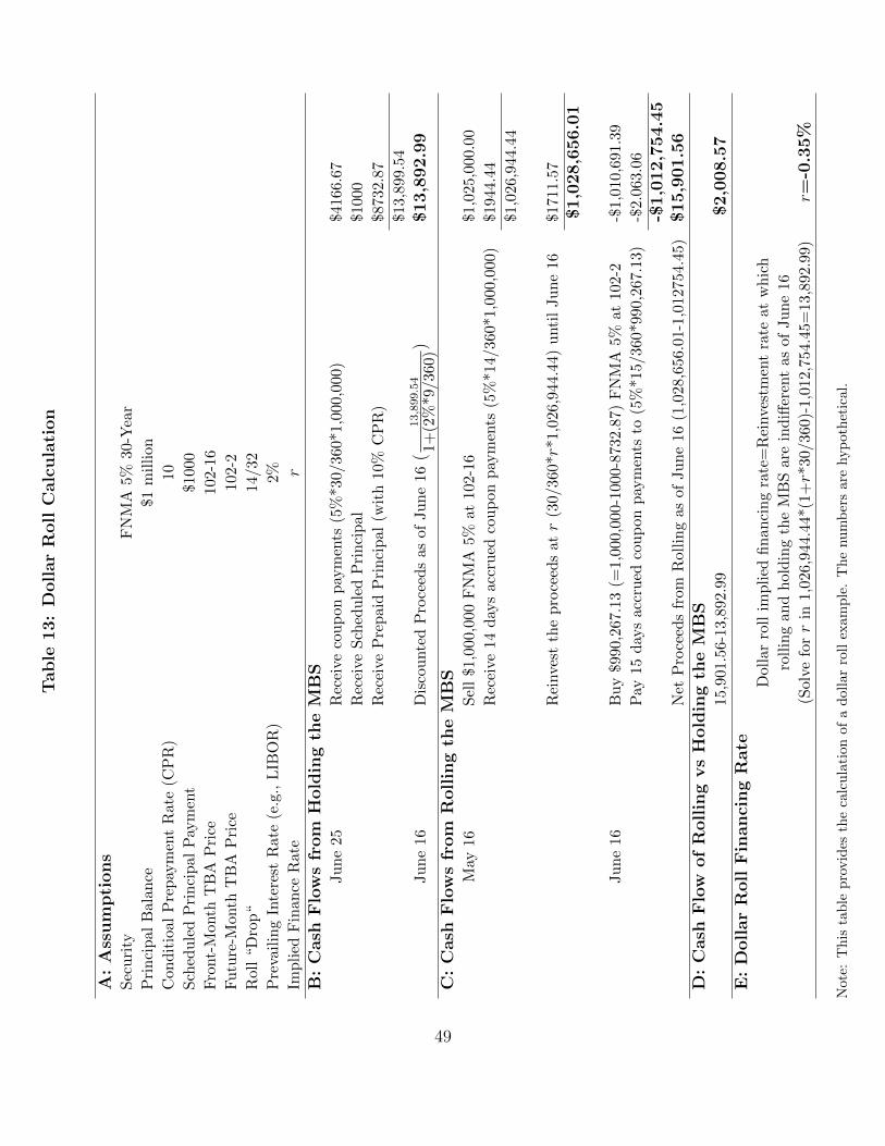
Table

13:

Doll

ar

Roll

Calc

ula

tion

A:

Ass

um

pti

on

sS

ecu

rity

FN

MA

5%30

-Yea

r

Pri

nci

pal

Bal

ance

$1m

illi

on

Con

dit

ioal

Pre

pay

men

tR

ate

(CP

R)

10

Sch

edu

led

Pri

nci

pal

Pay

men

t$1

000

Fro

nt-

Month

TB

AP

rice

102-

16

Fu

ture

-Month

TB

AP

rice

102-

2

Rol

l“D

rop

“14

/32

Pre

vail

ing

Inte

rest

Rate

(e.g

.,L

IBO

R)

2%

Imp

lied

Fin

ance

Rat

er

B:

Cash

Flo

ws

from

Hold

ing

the

MB

SJu

ne

25

Rec

eive

cou

pon

pay

men

ts(5

%*3

0/36

0*1,

000,

000)

$416

6.67

Rec

eive

Sch

edu

led

Pri

nci

pal

$100

0

Rec

eive

Pre

pai

dP

rin

cip

al(w

ith

10%

CP

R)

$873

2.87

$13,

899.

54

Ju

ne

16D

isco

unte

dP

roce

eds

asof

Ju

ne

16(

13,899.54

1+(2

%*9

/360

))$13,8

92.9

9

C:

Cash

Flo

ws

from

Rollin

gth

eM

BS

May

16

Sel

l$1

,000

,000

FN

MA

5%at

102-

16$1

,025

,000

.00

Rec

eive

14d

ays

accr

ued

cou

pon

pay

men

ts(5

%*1

4/36

0*1,

000,

000)

$194

4.44

$1,0

26,9

44.4

4

Rei

nve

stth

ep

roce

eds

atr

(30/

360*r*

1,02

6,94

4.44

)u

nti

lJu

ne

16$1

711.

57

$1,0

28,6

56.0

1

Ju

ne

16

Bu

y$9

90,2

67.1

3(=

1,00

0,00

0-10

00-8

732.

87)

FN

MA

5%at

102-

2-$

1,01

0,69

1.39

Pay

15d

ays

accr

ued

cou

pon

pay

men

tsto

(5%

*15/

360*

990,

267.

13)

-$2.

063.

06

-$1,0

12,7

54.4

5N

etP

roce

eds

from

Rol

lin

gas

ofJu

ne

16(1

,028

,656

.01-

1,01

2754

.45)

$15,9

01.5

6D

:C

ash

Flo

wof

Rollin

gvs

Hold

ing

the

MB

S15

,901

.56-

13,8

92.9

9$2,0

08.5

7E

:D

ollar

Roll

Fin

an

cin

gR

ate

Dol

lar

roll

impli

edfi

nan

cin

gra

te=

Rei

nve

stm

ent

rate

atw

hic

h

roll

ing

and

hol

din

gth

eM

BS

are

ind

iffer

ent

asof

Ju

ne

16

(Sol

vefo

rr

in1,

026,

944.

44*(

1+r*

30/3

60)-

1,01

2,75

4.45

=13

,892

.99)

r=-0

.35%

Not

e:T

his

tab

lep

rovid

esth

eca

lcu

lati

onof

ad

oll

ar

roll

exam

ple

.T

he

nu

mb

ers

are

hyp

oth

etic

al.

49

References

Atanasov, V., and Merrick, J. 2012. Liquidity and value in the deep vs shallow ends of mortgage-backed securities pools. Working Paper.

Atanasov, V., Merrick, J., and Schuster, P. 2014. Why do dealers buy high and sell low? An analysisof persistent crossing in extremely segmented markets. working paper College of William andMary.

Banerjee, S., and Graveline, J. 2013. The Cost of Short-Selling Liquid Securities. Journal of Finance68: 637–664.

Belikoff, A., Levin, K., Stein, H., and Tian, X. 2010. Analysis of Mortgage-Backed Securities:Before and After the Credit Crisis. Bloomberg LP, Verson 2.2.

Bernanke, B. 2009. The Crisis and the Policy Response. Remarks at the Stamp Lecture, LondonSchool of Economics (London, England).

Bernanke, B. 2012. Monetary Policy since the Onset of the Crisis. Remarks at the Federal ReserveBank of Kansas City Economic Symposium (Jackson Hole, Wyoming).

Bessembinder, H., Maxwell, W., and Venkataraman, K. 2013. Trading activity and transactioncosts in structured credit products. Financial Analysts Journal 69(6): 55–68.

Boudoukh, J., Richardson, M., Stanton, R., and Whitelaw, R. 1997. Pricing mortgage-backedsecurities in a multifactor interest rate environment: A multivariate density estimation approach.Review of Financial Studies 10: 405–446.

Boyarchenko, N., Fuster, A., and Lucca, D. 2015. Understanding Mortgage Spreads. Federal ReserveBank of New York Staff Reports 674.

Buraschi, A., and Menini, D. 2002. Liquidity Risk and Specialness: How Well Do Forward RepoSpreads Price Future Specialness?. Journal of Financial Economics 64: 243–282.

Carlin, B., Longstaff, F., and Matoba, K. 2014. Disagreement and Asset Prices. Journal of FinancialEconomics 114: 226–238.

Cherian, J., Jacquier, E., and Jarrow, R. 2004. A Model of the Convenience Yields in On-the-RunTreasuries. Review of Derivatives Research 7: 79–97.

Chernov, M., Dunn, B., and Longstaff, F. 2015. Macroeconomic-driven Prepayment Risk and theValuation of Mortgage-Backed Securities. working paper UCLA.

Downing, C., Jaffee, D., and Wallace, N. 2009. Is the Market for Mortgage Backed Securities aMarket for Lemons?. Review of Financial Studies 22–7: 2457–2494.

Duarte, J., Longstaff, F., and Yu, F. 2007. Risk and Return in Fixed Income Arbitrage: Nickels inFront of a Steamroller?. Review of Financial Studies 20: 769–811.

Duffie, D. 1996. Special repo rates. Journal of Finance 51: 493–526.

50

Duffie, D., Garleanu, N., and Pedersen, L. H. 2002. Securities lending, shorting, and pricing. Journalof Financial Economics 66: 307–339.

Dunn, K., and McConnell, J. 1981. Valuation of GNMA mortgage-backed securities. Journal ofFinance 36: 599–616.

Fabozzi, F., and Mann, S. 2011. Handbook of Fixed Income Securities. McGraw-Hill; 8 edition.

Fleming, M., and Garbade, K. 2005. Explaining settlement fails. Current Issues in Economics andFinance, Federal Reserve Bank of New York 11.

Friewald, N., Jankowitsch, R., and Subrahmanyam, M. 2014. Transparency and liquidity in thestructured product market. working paper, WU Vienna University of Economics and Business.

Frost, J., Logan, L., Martin, A., McCabe, P., Natalucci, F., and Remache, J. 2015. Overnight RRPOperations as a Monetary Policy Tool: Some Design Considerations. Finance and EconomicsDiscussion Series 2015-010.

Gabaix, X., Krishnamurthy, A., and Vigneron, O. 2007. Limits of Arbitrage: Theory and Evidencefrom the Mortgage-Backed Securities Market. Journal of Finance 2: 557–595.

Gagnon, J., Raskin, M., Remanche, J., and Sack, B. 2011. The Financial Market Effects of theFederal Reserve Large-Scale Asset Purchases. International Journal of Central Banking 7-1: 3–44.

Gao, P., Schultz, P., and Song, Z. 2015. Liquidity in a Market for Unique Assets: Specified Pooland TBA Trading in the Mortgage Backed Securities Market. Working Paper.

Graveline, J. J., and McBrady, M. 2011. Who makes on-the-run Treasuries special?. Journal ofFinancial Intermediation 20: 620–632.

Hall, A. 2000. Controlling for Burnout in Estimating Mortgage Prepayment Models. Journal ofHousing Economics 9–4: 215–232.

Hancock, D., and Passmore, W. 2011. Did the Federal Reserve MBS Purchase Program LowerMortgage Rates?. Journal of Monetary Economics 58-5: 498–514.

Hansen, S. 2014. Mortgage Convexity. Journal of Financial Economics 113-2: 270–299.

Hayre, L. 2001. Salomon Smith Barney Guide to Mortgage-Backed and Asset-Backed Securities.Wiley.

Hayre, L., and Young, R. 2004. Guide to Mortage-Backed Securities. Technical report, Citigroup.

Himmelberg, C., Young, M., Shan, H., and Henson, C. 2013. The Impact of Fed MBS Purchaseson TBA Pool Quality. Goldman Sachs.

Hollifield, B., Neklyudov, A., and Spatt, C. 2014. Bid-ask spreads, trading networks, and the pricingof securitizations: 144a vs. registered securitizations. Working paper.

51

Jordan, B., and Jordan, S. 1997. Special repo rates: An empirical analysis. Journal of Finance 52:2051–2072.

Kandrac, J. 2013. Have Federal Reserve MBS Purchases Affected Market Functioning?. EconomicLetters 121: 188–191.

Kitsul, Y., and Ochoa, M. 2014. MBS Liquidity: Drivers and Risk Premiums. working paper, Boardof Governors of the Federal Reserve System.

Krishnamurthy, A. 2002. The bond/old-bond spread. Journal of Financial Economics 66: 463–506.

Krishnamurthy, A., and Vissing-Jorgensen, A. 2011. The Effects of Quantitative Easing on InterestRates: Channels and Implications for Policy. Brookings Papers on Economic Activity.

Krishnamurthy, A., and Vissing-Jorgensen, A. 2013. The Ins and Outs of LSAPs. Working paper.

Kupiec, P., and Kah, A. 1999. On the origin and interpretation of OAS. Journal of Fixed Income9: 82–92.

Malkhozov, A., Mueller, P., Vedolin, A., and Venter, G. 2013. Hedging in Fixed Income Markets.LSE Working Paper.

Pasquariello, P., and Vega, C. 2009. The on-the-Run Liquidity Phenomenon. Journal of FinancialEconomics 92-1: 1–24.

Schwartz, E., and Torous, W. 1989. Prepayment and the valuation of mortgage-backed securities.Journal of Finance 44: 375–392.

Stanton, R. 1995. Rational prepayment and the valuation of mortgage-backed securities. Review ofFinancial Studies 8: 677–708.

Stroebel, J., and Taylor, J. 2012. Estimated Impact of the Federal Reserve Mortgage-Backed Secu-rities Purchase Program. International Journal of Central Banking 8-2.

TMPG 2012. Margining in Agency MBS Trading. The Treasury Market Practices Group WhitePaper.

Vayanos, D., and Weill, P.-O. 2008. A search-based theory of the on-the-run phenomenon. Journalof Finance 63: 1361–1398.

Vickery, J., and Wright, J. 2011. TBA Trading and Liquidity in the Agency MBS Market. FederalReserve Bank of New York Economic Policy Review 19.

52

Mortgage Dollar Roll - Federal Reserve Bank of Atlanta

Documents

Transcript of Mortgage Dollar Roll - Federal Reserve Bank of Atlanta