U s e r G u i d e - Informatica Documentation... · 2018-07-27 · U s e r G u i d e - Informatica...
210
Informatica ® Big Data Management 10.2 User Guide
Transcript of U s e r G u i d e - Informatica Documentation... · 2018-07-27 · U s e r G u i d e - Informatica...
Informatica® Big Data Management10.2
User Guide
Informatica Big Data Management User Guide10.2September 2017
© Copyright Informatica LLC 2012, 2018
This software and documentation are provided only under a separate license agreement containing restrictions on use and disclosure. No part of this document may be reproduced or transmitted in any form, by any means (electronic, photocopying, recording or otherwise) without prior consent of Informatica LLC.
Informatica, the Informatica logo, Big Data Management, and PowerExchange are trademarks or registered trademarks of Informatica LLC in the United States and many jurisdictions throughout the world. A current list of Informatica trademarks is available on the web at https://www.informatica.com/trademarks.html. Other company and product names may be trade names or trademarks of their respective owners.
Portions of this software and/or documentation are subject to copyright held by third parties, including without limitation: Copyright DataDirect Technologies. All rights reserved. Copyright © Sun Microsystems. All rights reserved. Copyright © RSA Security Inc. All Rights Reserved. Copyright © Ordinal Technology Corp. All rights reserved. Copyright © Aandacht c.v. All rights reserved. Copyright Genivia, Inc. All rights reserved. Copyright Isomorphic Software. All rights reserved. Copyright © Meta Integration Technology, Inc. All rights reserved. Copyright © Intalio. All rights reserved. Copyright © Oracle. All rights reserved. Copyright © Adobe Systems Incorporated. All rights reserved. Copyright © DataArt, Inc. All rights reserved. Copyright © ComponentSource. All rights reserved. Copyright © Microsoft Corporation. All rights reserved. Copyright © Rogue Wave Software, Inc. All rights reserved. Copyright © Teradata Corporation. All rights reserved. Copyright © Yahoo! Inc. All rights reserved. Copyright © Glyph & Cog, LLC. All rights reserved. Copyright © Thinkmap, Inc. All rights reserved. Copyright © Clearpace Software Limited. All rights reserved. Copyright © Information Builders, Inc. All rights reserved. Copyright © OSS Nokalva, Inc. All rights reserved. Copyright Edifecs, Inc. All rights reserved. Copyright Cleo Communications, Inc. All rights reserved. Copyright © International Organization for Standardization 1986. All rights reserved. Copyright © ej-technologies GmbH. All rights reserved. Copyright © Jaspersoft Corporation. All rights reserved. Copyright © International Business Machines Corporation. All rights reserved. Copyright © yWorks GmbH. All rights reserved. Copyright © Lucent Technologies. All rights reserved. Copyright © University of Toronto. All rights reserved. Copyright © Daniel Veillard. All rights reserved. Copyright © Unicode, Inc. Copyright IBM Corp. All rights reserved. Copyright © MicroQuill Software Publishing, Inc. All rights reserved. Copyright © PassMark Software Pty Ltd. All rights reserved. Copyright © LogiXML, Inc. All rights reserved. Copyright © 2003-2010 Lorenzi Davide, All rights reserved. Copyright © Red Hat, Inc. All rights reserved. Copyright © The Board of Trustees of the Leland Stanford Junior University. All rights reserved. Copyright © EMC Corporation. All rights reserved. Copyright © Flexera Software. All rights reserved. Copyright © Jinfonet Software. All rights reserved. Copyright © Apple Inc. All rights reserved. Copyright © Telerik Inc. All rights reserved. Copyright © BEA Systems. All rights reserved. Copyright © PDFlib GmbH. All rights reserved. Copyright © Orientation in Objects GmbH. All rights reserved. Copyright © Tanuki Software, Ltd. All rights reserved. Copyright © Ricebridge. All rights reserved. Copyright © Sencha, Inc. All rights reserved. Copyright © Scalable Systems, Inc. All rights reserved. Copyright © jQWidgets. All rights reserved. Copyright © Tableau Software, Inc. All rights reserved. Copyright© MaxMind, Inc. All Rights Reserved. Copyright © TMate Software s.r.o. All rights reserved. Copyright © MapR Technologies Inc. All rights reserved. Copyright © Amazon Corporate LLC. All rights reserved. Copyright © Highsoft. All rights reserved. Copyright © Python Software Foundation. All rights reserved. Copyright © BeOpen.com. All rights reserved. Copyright © CNRI. All rights reserved.
This product includes software developed by the Apache Software Foundation (http://www.apache.org/), and/or other software which is licensed under various versions of the Apache License (the "License"). You may obtain a copy of these Licenses at http://www.apache.org/licenses/. Unless required by applicable law or agreed to in writing, software distributed under these Licenses is distributed on an "AS IS" BASIS, WITHOUT WARRANTIES OR CONDITIONS OF ANY KIND, either express or implied. See the Licenses for the specific language governing permissions and limitations under the Licenses.
This product includes software which was developed by Mozilla (http://www.mozilla.org/), software copyright The JBoss Group, LLC, all rights reserved; software copyright © 1999-2006 by Bruno Lowagie and Paulo Soares and other software which is licensed under various versions of the GNU Lesser General Public License Agreement, which may be found at http:// www.gnu.org/licenses/lgpl.html. The materials are provided free of charge by Informatica, "as-is", without warranty of any kind, either express or implied, including but not limited to the implied warranties of merchantability and fitness for a particular purpose.
The product includes ACE(TM) and TAO(TM) software copyrighted by Douglas C. Schmidt and his research group at Washington University, University of California, Irvine, and Vanderbilt University, Copyright (©) 1993-2006, all rights reserved.
This product includes software developed by the OpenSSL Project for use in the OpenSSL Toolkit (copyright The OpenSSL Project. All Rights Reserved) and redistribution of this software is subject to terms available at http://www.openssl.org and http://www.openssl.org/source/license.html.
This product includes Curl software which is Copyright 1996-2013, Daniel Stenberg, <[email protected]>. All Rights Reserved. Permissions and limitations regarding this software are subject to terms available at http://curl.haxx.se/docs/copyright.html. Permission to use, copy, modify, and distribute this software for any purpose with or without fee is hereby granted, provided that the above copyright notice and this permission notice appear in all copies.
The product includes software copyright 2001-2005 (©) MetaStuff, Ltd. All Rights Reserved. Permissions and limitations regarding this software are subject to terms available at http://www.dom4j.org/ license.html.
The product includes software copyright © 2004-2007, The Dojo Foundation. All Rights Reserved. Permissions and limitations regarding this software are subject to terms available at http://dojotoolkit.org/license.
This product includes ICU software which is copyright International Business Machines Corporation and others. All rights reserved. Permissions and limitations regarding this software are subject to terms available at http://source.icu-project.org/repos/icu/icu/trunk/license.html.
This product includes software copyright © 1996-2006 Per Bothner. All rights reserved. Your right to use such materials is set forth in the license which may be found at http:// www.gnu.org/software/ kawa/Software-License.html.
This product includes OSSP UUID software which is Copyright © 2002 Ralf S. Engelschall, Copyright © 2002 The OSSP Project Copyright © 2002 Cable & Wireless Deutschland. Permissions and limitations regarding this software are subject to terms available at http://www.opensource.org/licenses/mit-license.php.
This product includes software developed by Boost (http://www.boost.org/) or under the Boost software license. Permissions and limitations regarding this software are subject to terms available at http:/ /www.boost.org/LICENSE_1_0.txt.
This product includes software copyright © 1997-2007 University of Cambridge. Permissions and limitations regarding this software are subject to terms available at http:// www.pcre.org/license.txt.
This product includes software copyright © 2007 The Eclipse Foundation. All Rights Reserved. Permissions and limitations regarding this software are subject to terms available at http:// www.eclipse.org/org/documents/epl-v10.php and at http://www.eclipse.org/org/documents/edl-v10.php.
This product includes software licensed under the terms at http://www.tcl.tk/software/tcltk/license.html, http://www.bosrup.com/web/overlib/?License, http://www.stlport.org/doc/ license.html, http://asm.ow2.org/license.html, http://www.cryptix.org/LICENSE.TXT, http://hsqldb.org/web/hsqlLicense.html, http://httpunit.sourceforge.net/doc/ license.html, http://jung.sourceforge.net/license.txt , http://www.gzip.org/zlib/zlib_license.html, http://www.openldap.org/software/release/license.html, http://www.libssh2.org, http://slf4j.org/license.html, http://www.sente.ch/software/OpenSourceLicense.html, http://fusesource.com/downloads/license-agreements/fuse-message-broker-v-5-3- license-agreement; http://antlr.org/license.html; http://aopalliance.sourceforge.net/; http://www.bouncycastle.org/licence.html; http://www.jgraph.com/jgraphdownload.html; http://www.jcraft.com/jsch/LICENSE.txt; http://jotm.objectweb.org/bsd_license.html; . http://www.w3.org/Consortium/Legal/2002/copyright-software-20021231; http://www.slf4j.org/license.html; http://nanoxml.sourceforge.net/orig/copyright.html; http://www.json.org/license.html; http://forge.ow2.org/projects/javaservice/, http://www.postgresql.org/about/licence.html, http://www.sqlite.org/copyright.html, http://www.tcl.tk/software/tcltk/license.html, http://www.jaxen.org/faq.html, http://www.jdom.org/docs/faq.html, http://www.slf4j.org/license.html; http://www.iodbc.org/dataspace/iodbc/wiki/iODBC/License; http://www.keplerproject.org/md5/license.html; http://www.toedter.com/en/jcalendar/license.html; http://www.edankert.com/bounce/index.html; http://www.net-snmp.org/about/license.html; http://www.openmdx.org/#FAQ; http://www.php.net/license/3_01.txt; http://srp.stanford.edu/license.txt;

http://www.schneier.com/blowfish.html; http://www.jmock.org/license.html; http://xsom.java.net; http://benalman.com/about/license/; https://github.com/CreateJS/EaselJS/blob/master/src/easeljs/display/Bitmap.js; http://www.h2database.com/html/license.html#summary; http://jsoncpp.sourceforge.net/LICENSE; http://jdbc.postgresql.org/license.html; http://protobuf.googlecode.com/svn/trunk/src/google/protobuf/descriptor.proto; https://github.com/rantav/hector/blob/master/LICENSE; http://web.mit.edu/Kerberos/krb5-current/doc/mitK5license.html; http://jibx.sourceforge.net/jibx-license.html; https://github.com/lyokato/libgeohash/blob/master/LICENSE; https://github.com/hjiang/jsonxx/blob/master/LICENSE; https://code.google.com/p/lz4/; https://github.com/jedisct1/libsodium/blob/master/LICENSE; http://one-jar.sourceforge.net/index.php?page=documents&file=license; https://github.com/EsotericSoftware/kryo/blob/master/license.txt; http://www.scala-lang.org/license.html; https://github.com/tinkerpop/blueprints/blob/master/LICENSE.txt; http://gee.cs.oswego.edu/dl/classes/EDU/oswego/cs/dl/util/concurrent/intro.html; https://aws.amazon.com/asl/; https://github.com/twbs/bootstrap/blob/master/LICENSE; https://sourceforge.net/p/xmlunit/code/HEAD/tree/trunk/LICENSE.txt; https://github.com/documentcloud/underscore-contrib/blob/master/LICENSE, and https://github.com/apache/hbase/blob/master/LICENSE.txt.
This product includes software licensed under the Academic Free License (http://www.opensource.org/licenses/afl-3.0.php), the Common Development and Distribution License (http://www.opensource.org/licenses/cddl1.php) the Common Public License (http://www.opensource.org/licenses/cpl1.0.php), the Sun Binary Code License Agreement Supplemental License Terms, the BSD License (http:// www.opensource.org/licenses/bsd-license.php), the new BSD License (http://opensource.org/licenses/BSD-3-Clause), the MIT License (http://www.opensource.org/licenses/mit-license.php), the Artistic License (http://www.opensource.org/licenses/artistic-license-1.0) and the Initial Developer’s Public License Version 1.0 (http://www.firebirdsql.org/en/initial-developer-s-public-license-version-1-0/).
This product includes software copyright © 2003-2006 Joe WaInes, 2006-2007 XStream Committers. All rights reserved. Permissions and limitations regarding this software are subject to terms available at http://xstream.codehaus.org/license.html. This product includes software developed by the Indiana University Extreme! Lab. For further information please visit http://www.extreme.indiana.edu/.
This product includes software Copyright (c) 2013 Frank Balluffi and Markus Moeller. All rights reserved. Permissions and limitations regarding this software are subject to terms of the MIT license.
See patents at https://www.informatica.com/legal/patents.html.
DISCLAIMER: Informatica LLC provides this documentation "as is" without warranty of any kind, either express or implied, including, but not limited to, the implied warranties of noninfringement, merchantability, or use for a particular purpose. Informatica LLC does not warrant that this software or documentation is error free. The information provided in this software or documentation may include technical inaccuracies or typographical errors. The information in this software and documentation is subject to change at any time without notice.
NOTICES
This Informatica product (the "Software") includes certain drivers (the "DataDirect Drivers") from DataDirect Technologies, an operating company of Progress Software Corporation ("DataDirect") which are subject to the following terms and conditions:
1. THE DATADIRECT DRIVERS ARE PROVIDED "AS IS" WITHOUT WARRANTY OF ANY KIND, EITHER EXPRESSED OR IMPLIED, INCLUDING BUT NOT LIMITED TO, THE IMPLIED WARRANTIES OF MERCHANTABILITY, FITNESS FOR A PARTICULAR PURPOSE AND NON-INFRINGEMENT.
2. IN NO EVENT WILL DATADIRECT OR ITS THIRD PARTY SUPPLIERS BE LIABLE TO THE END-USER CUSTOMER FOR ANY DIRECT, INDIRECT, INCIDENTAL, SPECIAL, CONSEQUENTIAL OR OTHER DAMAGES ARISING OUT OF THE USE OF THE ODBC DRIVERS, WHETHER OR NOT INFORMED OF THE POSSIBILITIES OF DAMAGES IN ADVANCE. THESE LIMITATIONS APPLY TO ALL CAUSES OF ACTION, INCLUDING, WITHOUT LIMITATION, BREACH OF CONTRACT, BREACH OF WARRANTY, NEGLIGENCE, STRICT LIABILITY, MISREPRESENTATION AND OTHER TORTS.
The information in this documentation is subject to change without notice. If you find any problems in this documentation, report them to us at [email protected].
Informatica products are warranted according to the terms and conditions of the agreements under which they are provided. INFORMATICA PROVIDES THE INFORMATION IN THIS DOCUMENT "AS IS" WITHOUT WARRANTY OF ANY KIND, EXPRESS OR IMPLIED, INCLUDING WITHOUT ANY WARRANTIES OF MERCHANTABILITY, FITNESS FOR A PARTICULAR PURPOSE AND ANY WARRANTY OR CONDITION OF NON-INFRINGEMENT.
Revision: 1Publication Date: 2018-07-27

Table of Contents
Preface . . . . . . . . . . . . . . . . . . . . . . . . . . . . . . . . . . . . . . . . . . . . . . . . . . . . . . . . . . . . . . . . . . . . . 10Informatica Resources. . . . . . . . . . . . . . . . . . . . . . . . . . . . . . . . . . . . . . . . . . . . . . . . . . 10
Informatica Network. . . . . . . . . . . . . . . . . . . . . . . . . . . . . . . . . . . . . . . . . . . . . . . . . 10
Informatica Knowledge Base. . . . . . . . . . . . . . . . . . . . . . . . . . . . . . . . . . . . . . . . . . . 10
Informatica Documentation. . . . . . . . . . . . . . . . . . . . . . . . . . . . . . . . . . . . . . . . . . . . 10
Informatica Product Availability Matrixes. . . . . . . . . . . . . . . . . . . . . . . . . . . . . . . . . . . 11
Informatica Velocity. . . . . . . . . . . . . . . . . . . . . . . . . . . . . . . . . . . . . . . . . . . . . . . . . 11
Informatica Marketplace. . . . . . . . . . . . . . . . . . . . . . . . . . . . . . . . . . . . . . . . . . . . . . 11
Informatica Global Customer Support. . . . . . . . . . . . . . . . . . . . . . . . . . . . . . . . . . . . . . 11
Chapter 1: Introduction to Informatica Big Data Management. . . . . . . . . . . . . . . . 12Informatica Big Data Management Overview. . . . . . . . . . . . . . . . . . . . . . . . . . . . . . . . . . . . 12
Example. . . . . . . . . . . . . . . . . . . . . . . . . . . . . . . . . . . . . . . . . . . . . . . . . . . . . . . . 13
Big Data Management Tasks . . . . . . . . . . . . . . . . . . . . . . . . . . . . . . . . . . . . . . . . . . . . . . 13
Read from and Write to Big Data Sources and Targets. . . . . . . . . . . . . . . . . . . . . . . . . . . 13
Perform Data Discovery. . . . . . . . . . . . . . . . . . . . . . . . . . . . . . . . . . . . . . . . . . . . . . . 14
Perform Data Lineage on Big Data Sources. . . . . . . . . . . . . . . . . . . . . . . . . . . . . . . . . . 15
Stream Machine Data. . . . . . . . . . . . . . . . . . . . . . . . . . . . . . . . . . . . . . . . . . . . . . . . 15
Process Streamed Data in Real Time. . . . . . . . . . . . . . . . . . . . . . . . . . . . . . . . . . . . . . 15
Manage Big Data Relationships. . . . . . . . . . . . . . . . . . . . . . . . . . . . . . . . . . . . . . . . . . 15
Big Data Management Component Architecture. . . . . . . . . . . . . . . . . . . . . . . . . . . . . . . . . . 16
Clients and Tools. . . . . . . . . . . . . . . . . . . . . . . . . . . . . . . . . . . . . . . . . . . . . . . . . . . 16
Application Services. . . . . . . . . . . . . . . . . . . . . . . . . . . . . . . . . . . . . . . . . . . . . . . . . 17
Repositories. . . . . . . . . . . . . . . . . . . . . . . . . . . . . . . . . . . . . . . . . . . . . . . . . . . . . . 17
Hadoop Environment. . . . . . . . . . . . . . . . . . . . . . . . . . . . . . . . . . . . . . . . . . . . . . . . 18
Hadoop Utilities. . . . . . . . . . . . . . . . . . . . . . . . . . . . . . . . . . . . . . . . . . . . . . . . . . . . 18
Big Data Management Engines. . . . . . . . . . . . . . . . . . . . . . . . . . . . . . . . . . . . . . . . . . . . . 19
Blaze Engine Architecture. . . . . . . . . . . . . . . . . . . . . . . . . . . . . . . . . . . . . . . . . . . . . 19
Spark Engine Architecture. . . . . . . . . . . . . . . . . . . . . . . . . . . . . . . . . . . . . . . . . . . . . 20
Hive Engine Architecture. . . . . . . . . . . . . . . . . . . . . . . . . . . . . . . . . . . . . . . . . . . . . . 21
Big Data Process. . . . . . . . . . . . . . . . . . . . . . . . . . . . . . . . . . . . . . . . . . . . . . . . . . . . . . 22
Step 1. Collect the Data. . . . . . . . . . . . . . . . . . . . . . . . . . . . . . . . . . . . . . . . . . . . . . . 23
Step 2. Cleanse the Data. . . . . . . . . . . . . . . . . . . . . . . . . . . . . . . . . . . . . . . . . . . . . . 23
Step 3. Transform the Data. . . . . . . . . . . . . . . . . . . . . . . . . . . . . . . . . . . . . . . . . . . . 23
Step 4. Process the Data. . . . . . . . . . . . . . . . . . . . . . . . . . . . . . . . . . . . . . . . . . . . . . 23
Step 5. Monitor Jobs. . . . . . . . . . . . . . . . . . . . . . . . . . . . . . . . . . . . . . . . . . . . . . . . 23
Chapter 2: Connections. . . . . . . . . . . . . . . . . . . . . . . . . . . . . . . . . . . . . . . . . . . . . . . . . . . . . 24Connections. . . . . . . . . . . . . . . . . . . . . . . . . . . . . . . . . . . . . . . . . . . . . . . . . . . . . . . . . 24
Hadoop Connection Properties. . . . . . . . . . . . . . . . . . . . . . . . . . . . . . . . . . . . . . . . . . . . . 25
4 Table of Contents
HDFS Connection Properties. . . . . . . . . . . . . . . . . . . . . . . . . . . . . . . . . . . . . . . . . . . . . . 29
HBase Connection Properties. . . . . . . . . . . . . . . . . . . . . . . . . . . . . . . . . . . . . . . . . . . . . . 31
HBase Connection Properties for MapR-DB. . . . . . . . . . . . . . . . . . . . . . . . . . . . . . . . . . . . . 32
Hive Connection Properties. . . . . . . . . . . . . . . . . . . . . . . . . . . . . . . . . . . . . . . . . . . . . . . 32
JDBC Connection Properties. . . . . . . . . . . . . . . . . . . . . . . . . . . . . . . . . . . . . . . . . . . . . . 37
Sqoop Connection-Level Arguments. . . . . . . . . . . . . . . . . . . . . . . . . . . . . . . . . . . . . . . 40
Creating a Connection to Access Sources or Targets. . . . . . . . . . . . . . . . . . . . . . . . . . . . . . . 42
Creating a Hadoop Connection. . . . . . . . . . . . . . . . . . . . . . . . . . . . . . . . . . . . . . . . . . . . . 43
Chapter 3: Mappings in the Hadoop Environment. . . . . . . . . . . . . . . . . . . . . . . . . . . . 44Mappings in the Hadoop Environment Overview. . . . . . . . . . . . . . . . . . . . . . . . . . . . . . . . . . 44
Mapping Run-time Properties. . . . . . . . . . . . . . . . . . . . . . . . . . . . . . . . . . . . . . . . . . . . . . 45
Validation Environments. . . . . . . . . . . . . . . . . . . . . . . . . . . . . . . . . . . . . . . . . . . . . . 45
Execution Environment. . . . . . . . . . . . . . . . . . . . . . . . . . . . . . . . . . . . . . . . . . . . . . . 46
Updating Run-time Properties for Multiple Mappings. . . . . . . . . . . . . . . . . . . . . . . . . . . . 48
Data Warehouse Optimization Mapping Example . . . . . . . . . . . . . . . . . . . . . . . . . . . . . . . . . 48
Sqoop Mappings in a Hadoop Environment. . . . . . . . . . . . . . . . . . . . . . . . . . . . . . . . . . . . . 50
Sqoop Mapping-Level Arguments. . . . . . . . . . . . . . . . . . . . . . . . . . . . . . . . . . . . . . . . 51
Configuring Sqoop Properties in the Mapping. . . . . . . . . . . . . . . . . . . . . . . . . . . . . . . . . 52
Rules and Guidelines for Mappings in a Hadoop Environment. . . . . . . . . . . . . . . . . . . . . . . . . 53
Workflows that Run Mappings in a Hadoop Environment. . . . . . . . . . . . . . . . . . . . . . . . . . . . 53
Configuring a Mapping to Run in a Hadoop Environment. . . . . . . . . . . . . . . . . . . . . . . . . . . . . 54
Mapping Execution Plans. . . . . . . . . . . . . . . . . . . . . . . . . . . . . . . . . . . . . . . . . . . . . . . . 54
Blaze Engine Execution Plan Details. . . . . . . . . . . . . . . . . . . . . . . . . . . . . . . . . . . . . . . 55
Spark Engine Execution Plan Details. . . . . . . . . . . . . . . . . . . . . . . . . . . . . . . . . . . . . . 56
Hive Engine Execution Plan Details. . . . . . . . . . . . . . . . . . . . . . . . . . . . . . . . . . . . . . . 57
Viewing the Execution Plan for a Mapping in the Developer Tool. . . . . . . . . . . . . . . . . . . . . 57
Optimization for the Hadoop Environment. . . . . . . . . . . . . . . . . . . . . . . . . . . . . . . . . . . . . . 57
Blaze Engine High Availability. . . . . . . . . . . . . . . . . . . . . . . . . . . . . . . . . . . . . . . . . . . 58
Enabling Data Compression on Temporary Staging Tables. . . . . . . . . . . . . . . . . . . . . . . . 58
Parallel Sorting. . . . . . . . . . . . . . . . . . . . . . . . . . . . . . . . . . . . . . . . . . . . . . . . . . . . 59
Truncating Partitions in a Hive Target. . . . . . . . . . . . . . . . . . . . . . . . . . . . . . . . . . . . . . 60
Scheduling, Queuing, and Node Labeling. . . . . . . . . . . . . . . . . . . . . . . . . . . . . . . . . . . . 60
Troubleshooting a Mapping in a Hadoop Environment. . . . . . . . . . . . . . . . . . . . . . . . . . . . . . 62
Chapter 4: Mapping Objects in the Hadoop Environment. . . . . . . . . . . . . . . . . . . . . 63Sources in a Hadoop Environment. . . . . . . . . . . . . . . . . . . . . . . . . . . . . . . . . . . . . . . . . . . 63
Flat File Sources. . . . . . . . . . . . . . . . . . . . . . . . . . . . . . . . . . . . . . . . . . . . . . . . . . . 64
Hive Sources. . . . . . . . . . . . . . . . . . . . . . . . . . . . . . . . . . . . . . . . . . . . . . . . . . . . . 64
Complex File Sources. . . . . . . . . . . . . . . . . . . . . . . . . . . . . . . . . . . . . . . . . . . . . . . . 67
Relational Sources. . . . . . . . . . . . . . . . . . . . . . . . . . . . . . . . . . . . . . . . . . . . . . . . . . 67
Sqoop Sources. . . . . . . . . . . . . . . . . . . . . . . . . . . . . . . . . . . . . . . . . . . . . . . . . . . . 68
Targets in a Hadoop Environment. . . . . . . . . . . . . . . . . . . . . . . . . . . . . . . . . . . . . . . . . . . 69
Table of Contents 5
Flat File Targets. . . . . . . . . . . . . . . . . . . . . . . . . . . . . . . . . . . . . . . . . . . . . . . . . . . 69
HDFS Flat File Targets. . . . . . . . . . . . . . . . . . . . . . . . . . . . . . . . . . . . . . . . . . . . . . . 69
Hive Targets. . . . . . . . . . . . . . . . . . . . . . . . . . . . . . . . . . . . . . . . . . . . . . . . . . . . . . 70
Complex File Targets. . . . . . . . . . . . . . . . . . . . . . . . . . . . . . . . . . . . . . . . . . . . . . . . 72
Relational Targets. . . . . . . . . . . . . . . . . . . . . . . . . . . . . . . . . . . . . . . . . . . . . . . . . . 73
Sqoop Targets. . . . . . . . . . . . . . . . . . . . . . . . . . . . . . . . . . . . . . . . . . . . . . . . . . . . 73
Transformations in a Hadoop Environment. . . . . . . . . . . . . . . . . . . . . . . . . . . . . . . . . . . . . 74
Transformation Support on the Blaze Engine. . . . . . . . . . . . . . . . . . . . . . . . . . . . . . . . . 75
Transformation Support on the Spark Engine. . . . . . . . . . . . . . . . . . . . . . . . . . . . . . . . . 79
Transformation Support on the Hive Engine. . . . . . . . . . . . . . . . . . . . . . . . . . . . . . . . . . 81
Function and Data Type Processing. . . . . . . . . . . . . . . . . . . . . . . . . . . . . . . . . . . . . . . . . . 84
Rules and Guidelines for Spark Engine Processing. . . . . . . . . . . . . . . . . . . . . . . . . . . . . 85
Rules and Guidelines for Hive Engine Processing. . . . . . . . . . . . . . . . . . . . . . . . . . . . . . 86
Chapter 5: Processing Hierarchical Data on the Spark Engine. . . . . . . . . . . . . . . . 88Processing Hierarchical Data on the Spark Engine Overview. . . . . . . . . . . . . . . . . . . . . . . . . . 88
How to Develop a Mapping to Process Hierarchical Data. . . . . . . . . . . . . . . . . . . . . . . . . . . . 89
Complex Data Types. . . . . . . . . . . . . . . . . . . . . . . . . . . . . . . . . . . . . . . . . . . . . . . . . . . . 91
Array Data Type. . . . . . . . . . . . . . . . . . . . . . . . . . . . . . . . . . . . . . . . . . . . . . . . . . . . 92
Map Data Type. . . . . . . . . . . . . . . . . . . . . . . . . . . . . . . . . . . . . . . . . . . . . . . . . . . . 93
Struct Data Type. . . . . . . . . . . . . . . . . . . . . . . . . . . . . . . . . . . . . . . . . . . . . . . . . . . 94
Rules and Guidelines for Complex Data Types. . . . . . . . . . . . . . . . . . . . . . . . . . . . . . . . 95
Complex Ports. . . . . . . . . . . . . . . . . . . . . . . . . . . . . . . . . . . . . . . . . . . . . . . . . . . . . . . 96
Complex Ports in Transformations. . . . . . . . . . . . . . . . . . . . . . . . . . . . . . . . . . . . . . . . 97
Rules and Guidelines for Complex Ports. . . . . . . . . . . . . . . . . . . . . . . . . . . . . . . . . . . . 97
Creating a Complex Port. . . . . . . . . . . . . . . . . . . . . . . . . . . . . . . . . . . . . . . . . . . . . . 98
Complex Data Type Definitions. . . . . . . . . . . . . . . . . . . . . . . . . . . . . . . . . . . . . . . . . . . . . 98
Nested Data Type Definitions. . . . . . . . . . . . . . . . . . . . . . . . . . . . . . . . . . . . . . . . . . 100
Rules and Guidelines for Complex Data Type Definitions. . . . . . . . . . . . . . . . . . . . . . . . . 100
Creating a Complex Data Type Definition. . . . . . . . . . . . . . . . . . . . . . . . . . . . . . . . . . . 100
Importing a Complex Data Type Definition. . . . . . . . . . . . . . . . . . . . . . . . . . . . . . . . . . 101
Type Configuration. . . . . . . . . . . . . . . . . . . . . . . . . . . . . . . . . . . . . . . . . . . . . . . . . . . . 103
Changing the Type Configuration for an Array Port. . . . . . . . . . . . . . . . . . . . . . . . . . . . 103
Changing the Type Configuration for a Map Port. . . . . . . . . . . . . . . . . . . . . . . . . . . . . . 105
Specifying the Type Configuration for a Struct Port. . . . . . . . . . . . . . . . . . . . . . . . . . . . 106
Complex Operators. . . . . . . . . . . . . . . . . . . . . . . . . . . . . . . . . . . . . . . . . . . . . . . . . . . . 107
Extracting an Array Element Using a Subscript Operator. . . . . . . . . . . . . . . . . . . . . . . . . 108
Extracting a Struct Element Using the Dot Operator. . . . . . . . . . . . . . . . . . . . . . . . . . . . 108
Complex Functions. . . . . . . . . . . . . . . . . . . . . . . . . . . . . . . . . . . . . . . . . . . . . . . . . . . . 109
Hierarchical Data Conversion. . . . . . . . . . . . . . . . . . . . . . . . . . . . . . . . . . . . . . . . . . . . . 110
Convert Relational or Hierarchical Data to Struct Data. . . . . . . . . . . . . . . . . . . . . . . . . . 111
Convert Relational or Hierarchical Data to Nested Struct Data. . . . . . . . . . . . . . . . . . . . . 113
Extract Elements from Hierarchical Data. . . . . . . . . . . . . . . . . . . . . . . . . . . . . . . . . . . 120
6 Table of Contents

Flatten Hierarchical Data. . . . . . . . . . . . . . . . . . . . . . . . . . . . . . . . . . . . . . . . . . . . . 123
Chapter 6: Stateful Computing on the Spark Engine. . . . . . . . . . . . . . . . . . . . . . . . . 126Stateful Computing on the Spark Engine Overview. . . . . . . . . . . . . . . . . . . . . . . . . . . . . . . . 126
Windowing Configuration. . . . . . . . . . . . . . . . . . . . . . . . . . . . . . . . . . . . . . . . . . . . . . . . 127
Frame. . . . . . . . . . . . . . . . . . . . . . . . . . . . . . . . . . . . . . . . . . . . . . . . . . . . . . . . . 127
Partition and Order Keys. . . . . . . . . . . . . . . . . . . . . . . . . . . . . . . . . . . . . . . . . . . . . 128
Rules and Guidelines for Windowing Configuration. . . . . . . . . . . . . . . . . . . . . . . . . . . . 130
Window Functions. . . . . . . . . . . . . . . . . . . . . . . . . . . . . . . . . . . . . . . . . . . . . . . . . . . . 130
LEAD. . . . . . . . . . . . . . . . . . . . . . . . . . . . . . . . . . . . . . . . . . . . . . . . . . . . . . . . . . 131
LAG. . . . . . . . . . . . . . . . . . . . . . . . . . . . . . . . . . . . . . . . . . . . . . . . . . . . . . . . . . 131
Aggregate Functions as Window Functions. . . . . . . . . . . . . . . . . . . . . . . . . . . . . . . . . 131
Rules and Guidelines for Window Functions. . . . . . . . . . . . . . . . . . . . . . . . . . . . . . . . . 135
Windowing Examples. . . . . . . . . . . . . . . . . . . . . . . . . . . . . . . . . . . . . . . . . . . . . . . . . . 135
Financial Plans Example. . . . . . . . . . . . . . . . . . . . . . . . . . . . . . . . . . . . . . . . . . . . . 135
GPS Pings Example. . . . . . . . . . . . . . . . . . . . . . . . . . . . . . . . . . . . . . . . . . . . . . . . 137
Aggregate Function as Window Function Example. . . . . . . . . . . . . . . . . . . . . . . . . . . . . 139
Chapter 7: Monitoring Mappings in the Hadoop Environment. . . . . . . . . . . . . . . . 142Monitoring Mappings in the Hadoop Environment Overview. . . . . . . . . . . . . . . . . . . . . . . . . . 142
Hadoop Environment Logs. . . . . . . . . . . . . . . . . . . . . . . . . . . . . . . . . . . . . . . . . . . . . . . 142
YARN Web User Interface. . . . . . . . . . . . . . . . . . . . . . . . . . . . . . . . . . . . . . . . . . . . . 143
Accessing the Monitoring URL. . . . . . . . . . . . . . . . . . . . . . . . . . . . . . . . . . . . . . . . . 143
Viewing Hadoop Environment Logs in the Administrator Tool. . . . . . . . . . . . . . . . . . . . . . 144
Monitoring a Mapping. . . . . . . . . . . . . . . . . . . . . . . . . . . . . . . . . . . . . . . . . . . . . . . 145
Blaze Engine Monitoring. . . . . . . . . . . . . . . . . . . . . . . . . . . . . . . . . . . . . . . . . . . . . . . . 146
Blaze Job Monitoring Application. . . . . . . . . . . . . . . . . . . . . . . . . . . . . . . . . . . . . . . 147
Blaze Summary Report. . . . . . . . . . . . . . . . . . . . . . . . . . . . . . . . . . . . . . . . . . . . . . 148
Blaze Engine Logs. . . . . . . . . . . . . . . . . . . . . . . . . . . . . . . . . . . . . . . . . . . . . . . . . 152
Viewing Blaze Logs. . . . . . . . . . . . . . . . . . . . . . . . . . . . . . . . . . . . . . . . . . . . . . . . 153
Troubleshooting Blaze Monitoring. . . . . . . . . . . . . . . . . . . . . . . . . . . . . . . . . . . . . . . 154
Spark Engine Monitoring. . . . . . . . . . . . . . . . . . . . . . . . . . . . . . . . . . . . . . . . . . . . . . . . 154
Spark Engine Logs. . . . . . . . . . . . . . . . . . . . . . . . . . . . . . . . . . . . . . . . . . . . . . . . . 157
Viewing Spark Logs . . . . . . . . . . . . . . . . . . . . . . . . . . . . . . . . . . . . . . . . . . . . . . . . 157
Hive Engine Monitoring. . . . . . . . . . . . . . . . . . . . . . . . . . . . . . . . . . . . . . . . . . . . . . . . . 157
Hive Engine Logs. . . . . . . . . . . . . . . . . . . . . . . . . . . . . . . . . . . . . . . . . . . . . . . . . . 159
Chapter 8: Mappings in the Native Environment. . . . . . . . . . . . . . . . . . . . . . . . . . . . 160Mappings in the Native Environment Overview. . . . . . . . . . . . . . . . . . . . . . . . . . . . . . . . . . 160
Data Processor Mappings. . . . . . . . . . . . . . . . . . . . . . . . . . . . . . . . . . . . . . . . . . . . . . . 160
HDFS Mappings. . . . . . . . . . . . . . . . . . . . . . . . . . . . . . . . . . . . . . . . . . . . . . . . . . . . . . 161
HDFS Data Extraction Mapping Example. . . . . . . . . . . . . . . . . . . . . . . . . . . . . . . . . . . 161
Hive Mappings. . . . . . . . . . . . . . . . . . . . . . . . . . . . . . . . . . . . . . . . . . . . . . . . . . . . . . 162
Table of Contents 7
Hive Mapping Example. . . . . . . . . . . . . . . . . . . . . . . . . . . . . . . . . . . . . . . . . . . . . . 163
Social Media Mappings. . . . . . . . . . . . . . . . . . . . . . . . . . . . . . . . . . . . . . . . . . . . . . . . . 163
Twitter Mapping Example. . . . . . . . . . . . . . . . . . . . . . . . . . . . . . . . . . . . . . . . . . . . . 164
Chapter 9: Profiles. . . . . . . . . . . . . . . . . . . . . . . . . . . . . . . . . . . . . . . . . . . . . . . . . . . . . . . . . 165Profiles Overview. . . . . . . . . . . . . . . . . . . . . . . . . . . . . . . . . . . . . . . . . . . . . . . . . . . . . 165
Native Environment. . . . . . . . . . . . . . . . . . . . . . . . . . . . . . . . . . . . . . . . . . . . . . . . . . . 165
Hadoop Environment. . . . . . . . . . . . . . . . . . . . . . . . . . . . . . . . . . . . . . . . . . . . . . . . . . 166
Column Profiles for Sqoop Data Sources. . . . . . . . . . . . . . . . . . . . . . . . . . . . . . . . . . . 166
Creating a Single Data Object Profile in Informatica Developer. . . . . . . . . . . . . . . . . . . . . . . . 167
Creating an Enterprise Discovery Profile in Informatica Developer. . . . . . . . . . . . . . . . . . . . . . 168
Creating a Column Profile in Informatica Analyst. . . . . . . . . . . . . . . . . . . . . . . . . . . . . . . . . 169
Creating an Enterprise Discovery Profile in Informatica Analyst. . . . . . . . . . . . . . . . . . . . . . . 170
Creating a Scorecard in Informatica Analyst. . . . . . . . . . . . . . . . . . . . . . . . . . . . . . . . . . . . 171
Monitoring a Profile. . . . . . . . . . . . . . . . . . . . . . . . . . . . . . . . . . . . . . . . . . . . . . . . . . . 172
Troubleshooting. . . . . . . . . . . . . . . . . . . . . . . . . . . . . . . . . . . . . . . . . . . . . . . . . . . . . 172
Chapter 10: Native Environment Optimization. . . . . . . . . . . . . . . . . . . . . . . . . . . . . . 174Native Environment Optimization Overview. . . . . . . . . . . . . . . . . . . . . . . . . . . . . . . . . . . . 174
Processing Big Data on a Grid. . . . . . . . . . . . . . . . . . . . . . . . . . . . . . . . . . . . . . . . . . . . . 174
Data Integration Service Grid. . . . . . . . . . . . . . . . . . . . . . . . . . . . . . . . . . . . . . . . . . 175
Grid Optimization. . . . . . . . . . . . . . . . . . . . . . . . . . . . . . . . . . . . . . . . . . . . . . . . . . 175
Processing Big Data on Partitions. . . . . . . . . . . . . . . . . . . . . . . . . . . . . . . . . . . . . . . . . . 175
Partitioned Model Repository Mappings. . . . . . . . . . . . . . . . . . . . . . . . . . . . . . . . . . . 175
Partition Optimization. . . . . . . . . . . . . . . . . . . . . . . . . . . . . . . . . . . . . . . . . . . . . . . 176
High Availability. . . . . . . . . . . . . . . . . . . . . . . . . . . . . . . . . . . . . . . . . . . . . . . . . . . . . . 176
Appendix A: Data Type Reference. . . . . . . . . . . . . . . . . . . . . . . . . . . . . . . . . . . . . . . . . . 178Data Type Reference Overview. . . . . . . . . . . . . . . . . . . . . . . . . . . . . . . . . . . . . . . . . . . . 178
Transformation Data Type Support in a Hadoop Environment. . . . . . . . . . . . . . . . . . . . . . . . . 179
Complex File and Transformation Data Types. . . . . . . . . . . . . . . . . . . . . . . . . . . . . . . . . . . 179
Avro and Transformation Data Types. . . . . . . . . . . . . . . . . . . . . . . . . . . . . . . . . . . . . 180
JSON and Transformation Data Types. . . . . . . . . . . . . . . . . . . . . . . . . . . . . . . . . . . . 181
Parquet and Transformation Data Types. . . . . . . . . . . . . . . . . . . . . . . . . . . . . . . . . . . 181
Hive Data Types and Transformation Data Types. . . . . . . . . . . . . . . . . . . . . . . . . . . . . . . . 183
Hive Complex Data Types. . . . . . . . . . . . . . . . . . . . . . . . . . . . . . . . . . . . . . . . . . . . 184
Sqoop Data Types. . . . . . . . . . . . . . . . . . . . . . . . . . . . . . . . . . . . . . . . . . . . . . . . . . . . 185
Aurora Data Types. . . . . . . . . . . . . . . . . . . . . . . . . . . . . . . . . . . . . . . . . . . . . . . . . 185
IBM DB2 and DB2 for z/OS Data Types. . . . . . . . . . . . . . . . . . . . . . . . . . . . . . . . . . . . 185
Greenplum Data Types. . . . . . . . . . . . . . . . . . . . . . . . . . . . . . . . . . . . . . . . . . . . . . 186
Microsoft SQL Server Data Types. . . . . . . . . . . . . . . . . . . . . . . . . . . . . . . . . . . . . . . . 186
Netezza Data Types. . . . . . . . . . . . . . . . . . . . . . . . . . . . . . . . . . . . . . . . . . . . . . . . 187
Oracle Data Types. . . . . . . . . . . . . . . . . . . . . . . . . . . . . . . . . . . . . . . . . . . . . . . . . 187
8 Table of Contents
Teradata Data Types. . . . . . . . . . . . . . . . . . . . . . . . . . . . . . . . . . . . . . . . . . . . . . . . 188
Teradata Data Types with TDCH Specialized Connectors for Sqoop. . . . . . . . . . . . . . . . . . 188
Appendix B: Complex File Data Object Properties. . . . . . . . . . . . . . . . . . . . . . . . . . . 190Complex File Data Objects Overview. . . . . . . . . . . . . . . . . . . . . . . . . . . . . . . . . . . . . . . . . 190
Creating and Configuring a Complex File Data Object. . . . . . . . . . . . . . . . . . . . . . . . . . . . . . 190
Complex File Data Object Overview Properties. . . . . . . . . . . . . . . . . . . . . . . . . . . . . . . . . . 191
Compression and Decompression for Complex File Sources and Targets. . . . . . . . . . . . . . . . . 192
Parameterization of Complex File Data Objects. . . . . . . . . . . . . . . . . . . . . . . . . . . . . . . . . . 193
Complex File Data Object Read Properties. . . . . . . . . . . . . . . . . . . . . . . . . . . . . . . . . . . . . 194
General Properties. . . . . . . . . . . . . . . . . . . . . . . . . . . . . . . . . . . . . . . . . . . . . . . . . 194
Ports Properties. . . . . . . . . . . . . . . . . . . . . . . . . . . . . . . . . . . . . . . . . . . . . . . . . . . 194
Sources Properties. . . . . . . . . . . . . . . . . . . . . . . . . . . . . . . . . . . . . . . . . . . . . . . . . 194
Advanced Properties. . . . . . . . . . . . . . . . . . . . . . . . . . . . . . . . . . . . . . . . . . . . . . . . 195
Column Projection Properties. . . . . . . . . . . . . . . . . . . . . . . . . . . . . . . . . . . . . . . . . . 196
Complex File Data Object Write Properties. . . . . . . . . . . . . . . . . . . . . . . . . . . . . . . . . . . . . 196
General Properties. . . . . . . . . . . . . . . . . . . . . . . . . . . . . . . . . . . . . . . . . . . . . . . . . 196
Port Properties. . . . . . . . . . . . . . . . . . . . . . . . . . . . . . . . . . . . . . . . . . . . . . . . . . . 197
Sources Properties. . . . . . . . . . . . . . . . . . . . . . . . . . . . . . . . . . . . . . . . . . . . . . . . . 197
Advanced Properties. . . . . . . . . . . . . . . . . . . . . . . . . . . . . . . . . . . . . . . . . . . . . . . . 197
Column Projection Properties. . . . . . . . . . . . . . . . . . . . . . . . . . . . . . . . . . . . . . . . . . 199
Appendix C: Function Reference. . . . . . . . . . . . . . . . . . . . . . . . . . . . . . . . . . . . . . . . . . . . 200Function Support in a Hadoop Environment. . . . . . . . . . . . . . . . . . . . . . . . . . . . . . . . . . . . 200
Appendix D: Parameter Reference. . . . . . . . . . . . . . . . . . . . . . . . . . . . . . . . . . . . . . . . . . 203Parameters Overview. . . . . . . . . . . . . . . . . . . . . . . . . . . . . . . . . . . . . . . . . . . . . . . . . . 203
Parameter Usage. . . . . . . . . . . . . . . . . . . . . . . . . . . . . . . . . . . . . . . . . . . . . . . . . . . . . 204
Index. . . . . . . . . . . . . . . . . . . . . . . . . . . . . . . . . . . . . . . . . . . . . . . . . . . . . . . . . . . 206
Table of Contents 9
PrefaceThe Informatica Big Data Management® User Guide provides information about configuring and running mappings in the native and Hadoop run-time environments.
Informatica Resources
Informatica NetworkInformatica Network hosts Informatica Global Customer Support, the Informatica Knowledge Base, and other product resources. To access Informatica Network, visit https://network.informatica.com.
As a member, you can:
• Access all of your Informatica resources in one place.
• Search the Knowledge Base for product resources, including documentation, FAQs, and best practices.
• View product availability information.
• Review your support cases.
• Find your local Informatica User Group Network and collaborate with your peers.
Informatica Knowledge BaseUse the Informatica Knowledge Base to search Informatica Network for product resources such as documentation, how-to articles, best practices, and PAMs.
To access the Knowledge Base, visit https://kb.informatica.com. If you have questions, comments, or ideas about the Knowledge Base, contact the Informatica Knowledge Base team at [email protected].
Informatica DocumentationTo get the latest documentation for your product, browse the Informatica Knowledge Base at https://kb.informatica.com/_layouts/ProductDocumentation/Page/ProductDocumentSearch.aspx.
If you have questions, comments, or ideas about this documentation, contact the Informatica Documentation team through email at [email protected].
10
Informatica Product Availability MatrixesProduct Availability Matrixes (PAMs) indicate the versions of operating systems, databases, and other types of data sources and targets that a product release supports. If you are an Informatica Network member, you can access PAMs at https://network.informatica.com/community/informatica-network/product-availability-matrices.
Informatica VelocityInformatica Velocity is a collection of tips and best practices developed by Informatica Professional Services. Developed from the real-world experience of hundreds of data management projects, Informatica Velocity represents the collective knowledge of our consultants who have worked with organizations from around the world to plan, develop, deploy, and maintain successful data management solutions.
If you are an Informatica Network member, you can access Informatica Velocity resources at http://velocity.informatica.com.
If you have questions, comments, or ideas about Informatica Velocity, contact Informatica Professional Services at [email protected].
Informatica MarketplaceThe Informatica Marketplace is a forum where you can find solutions that augment, extend, or enhance your Informatica implementations. By leveraging any of the hundreds of solutions from Informatica developers and partners, you can improve your productivity and speed up time to implementation on your projects. You can access Informatica Marketplace at https://marketplace.informatica.com.
Informatica Global Customer SupportYou can contact a Global Support Center by telephone or through Online Support on Informatica Network.
To find your local Informatica Global Customer Support telephone number, visit the Informatica website at the following link: http://www.informatica.com/us/services-and-training/support-services/global-support-centers.
If you are an Informatica Network member, you can use Online Support at http://network.informatica.com.
Preface 11
C h a p t e r 1
Introduction to Informatica Big Data Management
This chapter includes the following topics:
• Informatica Big Data Management Overview, 12
• Big Data Management Tasks , 13
• Big Data Management Component Architecture, 16
• Big Data Management Engines, 19
• Big Data Process, 22
Informatica Big Data Management OverviewInformatica Big Data Management enables your organization to process large, diverse, and fast changing data sets so you can get insights into your data. Use Big Data Management to perform big data integration and transformation without writing or maintaining Apache Hadoop code.
Use Big Data Management to collect diverse data faster, build business logic in a visual environment, and eliminate hand-coding to get insights on your data. Consider implementing a big data project in the following situations:
• The volume of the data that you want to process is greater than 10 terabytes.
• You need to analyze or capture data changes in microseconds.
• The data sources are varied and range from unstructured text to social media data.
You can identify big data sources and perform profiling to determine the quality of the data. You can build the business logic for the data and push this logic to the Hadoop cluster for faster and more efficient processing. You can view the status of the big data processing jobs and view how the big data queries are performing.
You can use multiple product tools and clients such as Informatica Developer (the Developer tool) and Informatica Administrator (the Administrator tool) to access big data functionality. Big Data Management connects to third-party applications such as the Hadoop Distributed File System (HDFS) and NoSQL databases such as HBase on a Hadoop cluster on different Hadoop distributions.
The Developer tool includes the native and Hadoop run-time environments for optimal processing. Use the native run-time environment to process data that is less than 10 terabytes. In the native environment, the Data Integration Service processes the data. The Hadoop run-time environment can optimize mapping performance and process data that is greater than 10 terabytes. In the Hadoop environment, the Data Integration Service pushes the processing to nodes in a Hadoop cluster.
12
When you run a mapping in the Hadoop environment, you can select to use the Spark engine, the Blaze engine, or the Hive engine to run the mapping.
ExampleYou are an investment banker who needs to calculate the popularity and risk of stocks and then match stocks to each customer based on the preferences of the customer. Your CIO wants to automate the process of calculating the popularity and risk of each stock, match stocks to each customer, and then send an email with a list of stock recommendations for all customers.
You consider the following requirements for your project:
• The volume of data generated by each stock is greater than 10 terabytes.
• You need to analyze the changes to the stock in microseconds.
• The stock is included in Twitter feeds and company stock trade websites, so you need to analyze these social media sources.
Based on your requirements, you work with the IT department to create mappings to determine the popularity of a stock. One mapping tracks the number of times the stock is included in Twitter feeds, and another mapping tracks the number of times customers inquire about the stock on the company stock trade website.
Big Data Management TasksUse Big Data Management when you want to access, analyze, prepare, transform, and stream data faster than traditional data processing environments.
You can use Big Data Management for the following tasks:
• Read from and write to diverse big data sources and targets.
• Perform data replication on a Hadoop cluster.
• Perform data discovery.
• Perform data lineage on big data sources.
• Stream machine data.
• Manage big data relationships.
Note: The Informatica Big Data Management User Guide describes how to run big data mappings in the native environment or the Hadoop environment. For information on specific license and configuration requirements for a task, refer to the related product guides.
Read from and Write to Big Data Sources and TargetsIn addition to relational and flat file data, you can access unstructured and semi-structured data, social media data, and data in a Hive or Hadoop Distributed File System (HDFS) environment.
You can access the following types of data:Transaction data
You can access different types of transaction data, including data from relational database management systems, online transaction processing systems, online analytical processing systems, enterprise resource planning systems, customer relationship management systems, mainframe, and cloud.
Big Data Management Tasks 13

Unstructured and semi-structured data
You can use parser transformations to read and transform unstructured and semi-structured data. For example, you can use the Data Processor transformation in a workflow to parse a Microsoft Word file to load customer and order data into relational database tables.
You can use HParser to transform complex data into flattened, usable formats for Hive, PIG, and MapReduce processing. HParser processes complex files, such as messaging formats, HTML pages and PDF documents. HParser also transforms formats such as ACORD, HIPAA, HL7, EDI-X12, EDIFACT, AFP, and SWIFT.
For more information, see the Data Transformation HParser Operator Guide.
Social media data
You can use PowerExchange® adapters for social media to read data from social media web sites like Facebook, Twitter, and LinkedIn. You can also use the PowerExchange for DataSift to extract real-time data from different social media web sites and capture data from DataSift regarding sentiment and language analysis. You can use PowerExchange for Web Content-Kapow to extract data from any web site.
Data in Hadoop
You can use PowerExchange adapters to read data from or write data to Hadoop. For example, you can use PowerExchange for Hive to read data from or write data to Hive. You can use PowerExchange for HDFS to extract data from and load data to HDFS. Also, you can use PowerExchange for HBase to extract data from and load data to HBase.
Data in Amazon Web Services
You can use PowerExchange adapters to read data from or write data to Amazon Web services. For example, you can use PowerExchange for Amazon Redshift to read data from or write data to Amazon Redshift. Also, you can use PowerExchange for Amazon S3 to extract data from and load data to Amazon S3.
For more information about PowerExchange adapters, see the related PowerExchange adapter guides.
Perform Data DiscoveryData discovery is the process of discovering the metadata of source systems that include content, structure, patterns, and data domains. Content refers to data values, frequencies, and data types. Structure includes candidate keys, primary keys, foreign keys, and functional dependencies. The data discovery process offers advanced profiling capabilities.
In the native environment, you can define a profile to analyze data in a single data object or across multiple data objects. In the Hadoop environment, you can push column profiles and the data domain discovery process to the Hadoop cluster.
Run a profile to evaluate the data structure and to verify that data columns contain the types of information you expect. You can drill down on data rows in profiled data. If the profile results reveal problems in the data, you can apply rules to fix the result set. You can create scorecards to track and measure data quality before and after you apply the rules. If the external source metadata of a profile or scorecard changes, you can synchronize the changes with its data object. You can add comments to profiles so that you can track the profiling process effectively.
For more information, see the Informatica Data Discovery Guide.
14 Chapter 1: Introduction to Informatica Big Data Management
Perform Data Lineage on Big Data SourcesPerform data lineage analysis in Enterprise Information Catalog for big data sources and targets.
Use Enterprise Information Catalog to create a Cloudera Navigator resource to extract metadata for big data sources and targets and perform data lineage analysis on the metadata. Cloudera Navigator is a data management tool for the Hadoop platform that enables users to track data access for entities and manage metadata about the entities in a Hadoop cluster.
You can create one Cloudera Navigator resource for each Hadoop cluster that is managed by Cloudera Manager. Enterprise Information Catalog extracts metadata about entities from the cluster based on the entity type.
Enterprise Information Catalog extracts metadata for the following entity types:
• HDFS files and directories
• Hive tables, query templates, and executions
• Oozie job templates and executions
• Pig tables, scripts, and script executions
• YARN job templates and executions
Note: Enterprise Information Catalog does not extract metadata for MapReduce job templates or executions.
For more information, see the Informatica Catalog Administrator Guide.
Stream Machine DataYou can stream machine data in real time. To stream machine data, use Informatica Vibe Data Stream for Machine Data (Vibe Data Stream).
Vibe Data Stream is a highly available, distributed, real-time application that collects and aggregates machine data. You can collect machine data from different types of sources and write to different types of targets. Vibe Data Stream consists of source services that collect data from sources and target services that aggregate and write data to a target.
For more information, see the Informatica Vibe Data Stream for Machine Data User Guide.
Process Streamed Data in Real TimeYou can process streamed data in real time. To process streams of data in real time and uncover insights in time to meet your business needs, use Informatica Intelligent Streaming.
Create Streaming mappings to collect the streamed data, build the business logic for the data, and push the logic to a Spark engine for processing. The Spark engine uses Spark Streaming to process data. The Spark engine reads the data, divides the data into micro batches and publishes it.
For more information, see the Informatica Intelligent Streaming User Guide.
Manage Big Data RelationshipsYou can manage big data relationships by integrating data from different sources and indexing and linking the data in a Hadoop environment. Use Big Data Management to integrate data from different sources. Then use the MDM Big Data Relationship Manager to index and link the data in a Hadoop environment.
MDM Big Data Relationship Manager indexes and links the data based on the indexing and matching rules. You can configure rules based on which to link the input records. MDM Big Data Relationship Manager uses the rules to match the input records and then group all the matched records. MDM Big Data Relationship
Big Data Management Tasks 15
Manager links all the matched records and creates a cluster for each group of the matched records. You can load the indexed and matched record into a repository.
For more information, see the MDM Big Data Relationship Management User Guide.
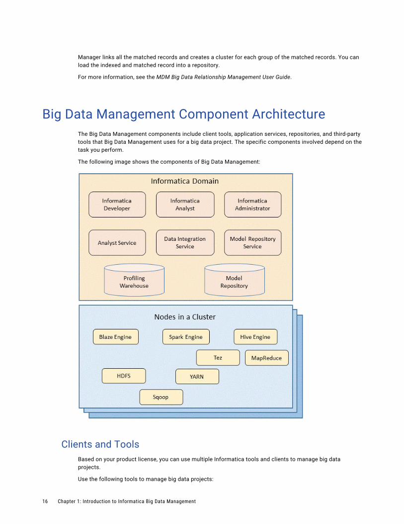
Big Data Management Component ArchitectureThe Big Data Management components include client tools, application services, repositories, and third-party tools that Big Data Management uses for a big data project. The specific components involved depend on the task you perform.
The following image shows the components of Big Data Management:
Clients and ToolsBased on your product license, you can use multiple Informatica tools and clients to manage big data projects.
Use the following tools to manage big data projects:
16 Chapter 1: Introduction to Informatica Big Data Management
Informatica Administrator
Monitor the status of profile, mapping, and MDM Big Data Relationship Management jobs on the Monitoring tab of the Administrator tool. The Monitoring tab of the Administrator tool is called the Monitoring tool. You can also design a Vibe Data Stream workflow in the Administrator tool.
Informatica Analyst
Create and run profiles on big data sources, and create mapping specifications to collaborate on projects and define business logic that populates a big data target with data.
Informatica Developer
Create and run profiles against big data sources, and run mappings and workflows on the Hadoop cluster from the Developer tool.
Application ServicesBig Data Management uses application services in the Informatica domain to process data.
Big Data Management uses the following application services:
Analyst Service
The Analyst Service runs the Analyst tool in the Informatica domain. The Analyst Service manages the connections between service components and the users that have access to the Analyst tool.
Data Integration Service
The Data Integration Service can process mappings in the native environment or push the mapping for processing to the Hadoop cluster in the Hadoop environment. The Data Integration Service also retrieves metadata from the Model repository when you run a Developer tool mapping or workflow. The Analyst tool and Developer tool connect to the Data Integration Service to run profile jobs and store profile results in the profiling warehouse.
Model Repository Service
The Model Repository Service manages the Model repository. The Model Repository Service connects to the Model repository when you run a mapping, mapping specification, profile, or workflow.
RepositoriesBig Data Management uses repositories and other databases to store data related to connections, source metadata, data domains, data profiling, data masking, and data lineage. Big Data Management uses application services in the Informatica domain to access data in repositories.
Big Data Management uses the following databases:
Model repository
The Model repository stores profiles, data domains, mapping, and workflows that you manage in the Developer tool. The Model repository also stores profiles, data domains, and mapping specifications that you manage in the Analyst tool.
Profiling warehouse
The Data Integration Service runs profiles and stores profile results in the profiling warehouse.
Big Data Management Component Architecture 17
Hadoop EnvironmentBig Data Management can connect to clusters that run different Hadoop distributions. Hadoop is an open-source software framework that enables distributed processing of large data sets across clusters of machines. You might also need to use third-party software clients to set up and manage your Hadoop cluster.
Big Data Management can connect to Hadoop as a data source and push job processing to the Hadoop cluster. It can also connect to HDFS, which enables high performance access to files across the cluster. It can connect to Hive, which is a data warehouse that connects to HDFS and uses SQL-like queries to run MapReduce jobs on Hadoop, or YARN, which can manage Hadoop clusters more efficiently. It can also connect to NoSQL databases such as HBase, which is a database comprising key-value pairs on Hadoop that performs operations in real-time.
The Data Integration Service pushes mapping and profiling jobs to the Blaze, Spark, or Hive engine in the Hadoop environment.
Hadoop UtilitiesBig Data Management uses third-party Hadoop utilities such as Sqoop to process data efficiently.
Sqoop is a Hadoop command line program to process data between relational databases and HDFS through MapReduce programs. You can use Sqoop to import and export data. When you use Sqoop, you do not need to install the relational database client and software on any node in the Hadoop cluster.
To use Sqoop, you must configure Sqoop properties in a JDBC connection and run the mapping in the Hadoop environment. You can configure Sqoop connectivity for relational data objects, customized data objects, and logical data objects that are based on a JDBC-compliant database. For example, you can configure Sqoop connectivity for the following databases:
• Aurora
• Greenplum
• IBM DB2
• IBM DB2 for z/OS
• Microsoft SQL Server
• Netezza
• Oracle
• Teradata
The Model Repository Service uses JDBC to import metadata. The Data Integration Service runs the mapping in the Hadoop run-time environment and pushes the job processing to Sqoop. Sqoop then creates map-reduce jobs in the Hadoop cluster, which perform the import and export job in parallel.
Specialized Sqoop Connectors
When you run mappings through Sqoop, you can use the following specialized connectors:
OraOop
You can use OraOop with Sqoop to optimize performance when you read data from or write data to Oracle. OraOop is a specialized Sqoop plug-in for Oracle that uses native protocols to connect to the Oracle database.
You can configure OraOop when you run Sqoop mappings on the Spark and Hive engines.
18 Chapter 1: Introduction to Informatica Big Data Management
Teradata Connector for Hadoop (TDCH) Specialized Connectors for Sqoop
You can use the following TDCH specialized connectors for Sqoop when you read data from or write data to Teradata:
• Cloudera Connector Powered by Teradata
• Hortonworks Connector for Teradata (powered by the Teradata Connector for Hadoop)
Cloudera Connector Powered by Teradata and Hortonworks Connector for Teradata are specialized Sqoop plug-ins that Cloudera and Hortonworks provide for Teradata. These TDCH Sqoop Connectors use native protocols to connect to the Teradata database.
You can configure the Cloudera Connector Powered by Teradata and Hortonworks Connector for Teradata when you run Sqoop mappings on the Blaze and Spark engines.
Note: For information about running native Teradata mappings with Sqoop, see the Informatica PowerExchange for Teradata Parallel Transporter API User Guide.
Big Data Management EnginesWhen you run a big data mapping, you can choose to run the mapping in the native environment or a Hadoop environment. If you run the mapping in a Hadoop environment, the mapping will run on the Blaze engine, the Spark engine, or the Hive engine.
When you validate a mapping, you can validate it against one or all of the engines. The Developer tool returns validation messages for each engine.
You can then choose to run the mapping in the native environment or in the Hadoop environment. When you run the mapping in the native environment, the Data Integration Service processes the mapping logic. When you run the mapping in the Hadoop environment, the Data Integration Service uses a proprietary rule-based methodology to determine the best engine to run the mapping. The rule-based methodology evaluates the mapping sources and the mapping logic to determine the engine. The Data Integration Service translates the mapping logic into code that the engine can process, and it transfers the code to the engine.
Blaze Engine ArchitectureTo run a mapping on the Informatica Blaze engine, the Data Integration Service submits jobs to the Blaze engine executor. The Blaze engine executor is a software component that enables communication between the Data Integration Service and the Blaze engine components on the Hadoop cluster.
The following Blaze engine components appear on the Hadoop cluster:
• Grid Manager. Manages tasks for batch processing.
• Orchestrator. Schedules and processes parallel data processing tasks on a cluster.
• Blaze Job Monitor. Monitors Blaze engine jobs on a cluster.
• DTM Process Manager. Manages the DTM Processes.
• DTM Processes. An operating system process started to run DTM instances.
• Data Exchange Framework. Shuffles data between different processes that process the data on cluster nodes.
Big Data Management Engines 19
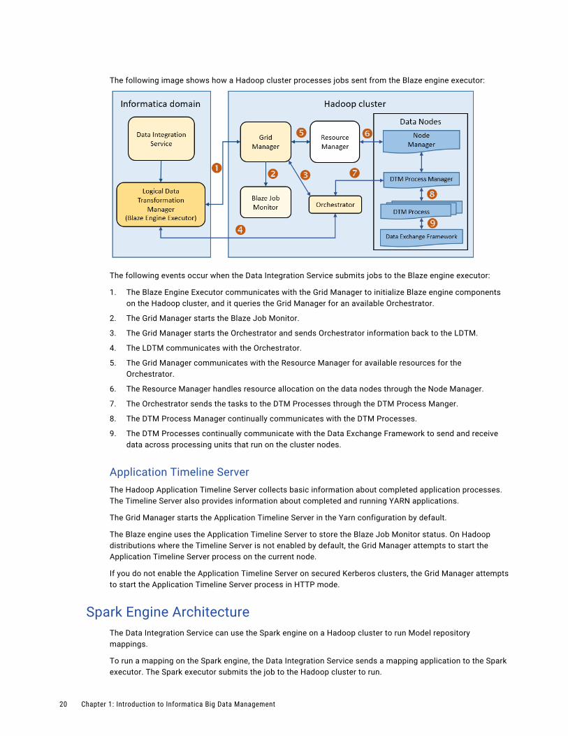
The following image shows how a Hadoop cluster processes jobs sent from the Blaze engine executor:
The following events occur when the Data Integration Service submits jobs to the Blaze engine executor:
1. The Blaze Engine Executor communicates with the Grid Manager to initialize Blaze engine components on the Hadoop cluster, and it queries the Grid Manager for an available Orchestrator.
2. The Grid Manager starts the Blaze Job Monitor.
3. The Grid Manager starts the Orchestrator and sends Orchestrator information back to the LDTM.
4. The LDTM communicates with the Orchestrator.
5. The Grid Manager communicates with the Resource Manager for available resources for the Orchestrator.
6. The Resource Manager handles resource allocation on the data nodes through the Node Manager.
7. The Orchestrator sends the tasks to the DTM Processes through the DTM Process Manger.
8. The DTM Process Manager continually communicates with the DTM Processes.
9. The DTM Processes continually communicate with the Data Exchange Framework to send and receive data across processing units that run on the cluster nodes.
Application Timeline ServerThe Hadoop Application Timeline Server collects basic information about completed application processes. The Timeline Server also provides information about completed and running YARN applications.
The Grid Manager starts the Application Timeline Server in the Yarn configuration by default.
The Blaze engine uses the Application Timeline Server to store the Blaze Job Monitor status. On Hadoop distributions where the Timeline Server is not enabled by default, the Grid Manager attempts to start the Application Timeline Server process on the current node.
If you do not enable the Application Timeline Server on secured Kerberos clusters, the Grid Manager attempts to start the Application Timeline Server process in HTTP mode.
Spark Engine ArchitectureThe Data Integration Service can use the Spark engine on a Hadoop cluster to run Model repository mappings.
To run a mapping on the Spark engine, the Data Integration Service sends a mapping application to the Spark executor. The Spark executor submits the job to the Hadoop cluster to run.
20 Chapter 1: Introduction to Informatica Big Data Management

The following image shows how a Hadoop cluster processes jobs sent from the Spark executor:
The following events occur when Data Integration Service runs a mapping on the Spark engine:
1. The Logical Data Transformation Manager translates the mapping into a Scala program, packages it as an application, and sends it to the Spark executor.
2. The Spark executor submits the application to the Resource Manager in the Hadoop cluster and requests resources to run the application.
Note: When you run mappings on the HDInsight cluster, the Spark executor launches a spark-submit script. The script requests resources to run the application.
3. The Resource Manager identifies the Node Managers that can provide resources, and it assigns jobs to the data nodes.
4. Driver and Executor processes are launched in data nodes where the Spark application runs.
Hive Engine ArchitectureThe Data Integration Service can use the Hive engine to run Model repository mappings or profiles on a Hadoop cluster.
To run a mapping or profile with the Hive engine, the Data Integration Service creates HiveQL queries based on the transformation or profiling logic. The Data Integration Service submits the HiveQL queries to the Hive driver. The Hive driver converts the HiveQL queries to MapReduce jobs, and then sends the jobs to the Hadoop cluster.
Big Data Management Engines 21
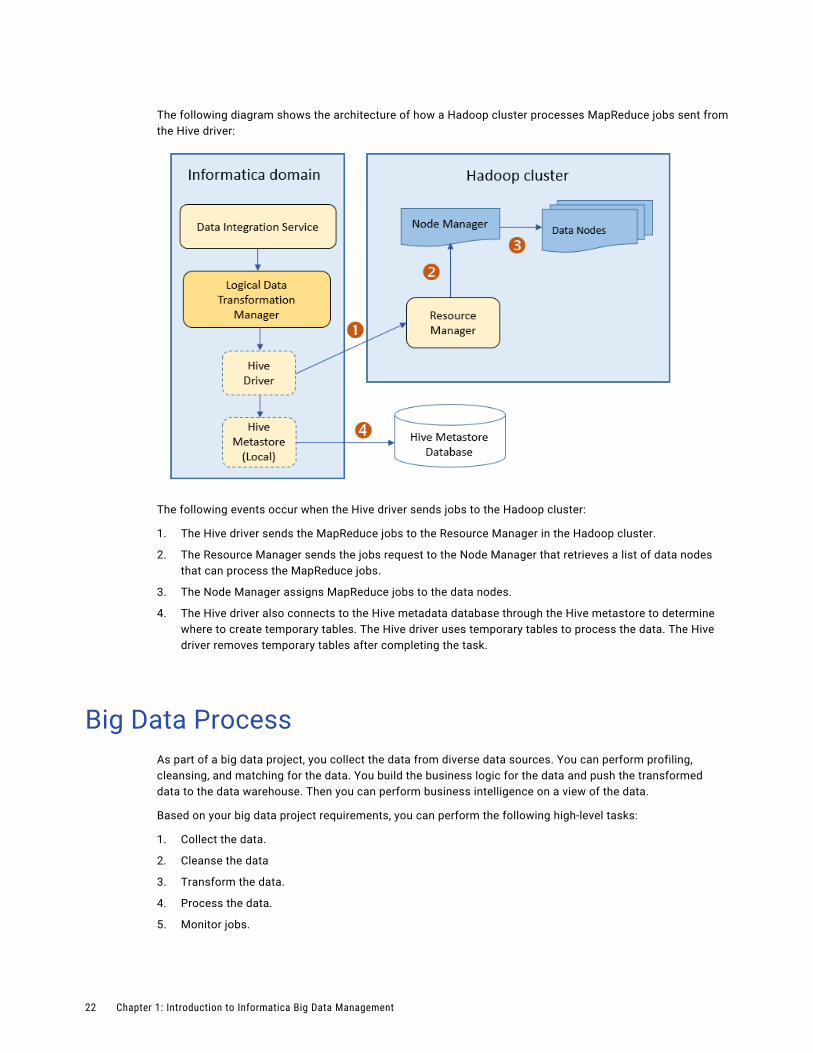
The following diagram shows the architecture of how a Hadoop cluster processes MapReduce jobs sent from the Hive driver:
The following events occur when the Hive driver sends jobs to the Hadoop cluster:
1. The Hive driver sends the MapReduce jobs to the Resource Manager in the Hadoop cluster.
2. The Resource Manager sends the jobs request to the Node Manager that retrieves a list of data nodes that can process the MapReduce jobs.
3. The Node Manager assigns MapReduce jobs to the data nodes.
4. The Hive driver also connects to the Hive metadata database through the Hive metastore to determine where to create temporary tables. The Hive driver uses temporary tables to process the data. The Hive driver removes temporary tables after completing the task.
Big Data ProcessAs part of a big data project, you collect the data from diverse data sources. You can perform profiling, cleansing, and matching for the data. You build the business logic for the data and push the transformed data to the data warehouse. Then you can perform business intelligence on a view of the data.
Based on your big data project requirements, you can perform the following high-level tasks:
1. Collect the data.
2. Cleanse the data
3. Transform the data.
4. Process the data.
5. Monitor jobs.
22 Chapter 1: Introduction to Informatica Big Data Management
Step 1. Collect the DataIdentify the data sources from which you need to collect the data.
Big Data Management provides several ways to access your data in and out of Hadoop based on the data types, data volumes, and data latencies in the data.
You can use PowerExchange adapters to connect to multiple big data sources. You can schedule batch loads to move data from multiple source systems to HDFS without the need to stage the data. You can move changed data from relational and mainframe systems into HDFS or the Hive warehouse. For real-time data feeds, you can move data off message queues and into HDFS.
You can collect the following types of data:
• Transactional
• Interactive
• Log file
• Sensor device
• Document and file
• Industry format
Step 2. Cleanse the DataCleanse the data by profiling, cleaning, and matching your data. You can view data lineage for the data.
You can perform data profiling to view missing values and descriptive statistics to identify outliers and anomalies in your data. You can view value and pattern frequencies to isolate inconsistencies or unexpected patterns in your data. You can drill down on the inconsistent data to view results across the entire data set.
You can automate the discovery of data domains and relationships between them. You can discover sensitive data such as social security numbers and credit card numbers so that you can mask the data for compliance.
After you are satisfied with the quality of your data, you can also create a business glossary from your data. You can use the Analyst tool or Developer tool to perform data profiling tasks. Use the Analyst tool to perform data discovery tasks. Use Metadata Manager to perform data lineage tasks.
Step 3. Transform the DataYou can build the business logic to parse data in the Developer tool. Eliminate the need for hand-coding the transformation logic by using pre-built Informatica transformations to transform data.
Step 4. Process the DataBased on your business logic, you can determine the optimal run-time environment to process your data. If your data is less than 10 terabytes, consider processing your data in the native environment. If your data is greater than 10 terabytes, consider processing your data in the Hadoop environment.
Step 5. Monitor JobsMonitor the status of your processing jobs. You can view monitoring statistics for your processing jobs in the Monitoring tool. After your processing jobs complete you can get business intelligence and analytics from your data.
Big Data Process 23
C h a p t e r 2
ConnectionsThis chapter includes the following topics:
• Connections, 24
• Hadoop Connection Properties, 25
• HDFS Connection Properties, 29
• HBase Connection Properties, 31
• HBase Connection Properties for MapR-DB, 32
• Hive Connection Properties, 32
• JDBC Connection Properties, 37
• Creating a Connection to Access Sources or Targets, 42
• Creating a Hadoop Connection, 43
ConnectionsDefine a Hadoop connection to run a mapping in the Hadoop environment. Depending on the sources and targets, define connections to access data in HBase, HDFS, Hive, or relational databases. You can create the connections using the Developer tool, Administrator tool, and infacmd.
You can create the following types of connections:Hadoop connection
Create a Hadoop connection to run mappings in the Hadoop environment. If you select the mapping validation environment or the execution environment as Hadoop, select the Hadoop connection. Before you run mappings in the Hadoop environment, review the information in this guide about rules and guidelines for mappings that you can run in the Hadoop environment.
HBase connection
Create an HBase connection to access HBase. The HBase connection is a NoSQL connection.
HDFS connection
Create an HDFS connection to read data from or write data to the HDFS file system on a Hadoop cluster.
Hive connection
Create a Hive connection to access Hive as a source or target. You can access Hive as a source if the mapping is enabled for the native or Hadoop environment. You can access Hive as a target if the mapping runs on the Blaze or Hive engine.
24
JDBC connection
Create a JDBC connection and configure Sqoop properties in the connection to import and export relational data through Sqoop.
Note: For information about creating connections to other sources or targets such as social media web sites or Teradata, see the respective PowerExchange adapter user guide for information.
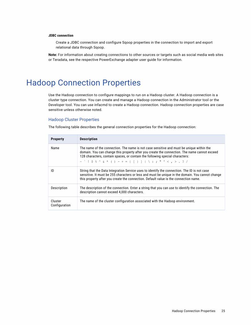
Hadoop Connection PropertiesUse the Hadoop connection to configure mappings to run on a Hadoop cluster. A Hadoop connection is a cluster type connection. You can create and manage a Hadoop connection in the Administrator tool or the Developer tool. You can use infacmd to create a Hadoop connection. Hadoop connection properties are case sensitive unless otherwise noted.
Hadoop Cluster Properties
The following table describes the general connection properties for the Hadoop connection:
Property Description
Name The name of the connection. The name is not case sensitive and must be unique within the domain. You can change this property after you create the connection. The name cannot exceed 128 characters, contain spaces, or contain the following special characters:~ ` ! $ % ^ & * ( ) - + = { [ } ] | \ : ; " ' < , > . ? /
ID String that the Data Integration Service uses to identify the connection. The ID is not case sensitive. It must be 255 characters or less and must be unique in the domain. You cannot change this property after you create the connection. Default value is the connection name.
Description The description of the connection. Enter a string that you can use to identify the connection. The description cannot exceed 4,000 characters.
Cluster Configuration
The name of the cluster configuration associated with the Hadoop environment.
Hadoop Connection Properties 25
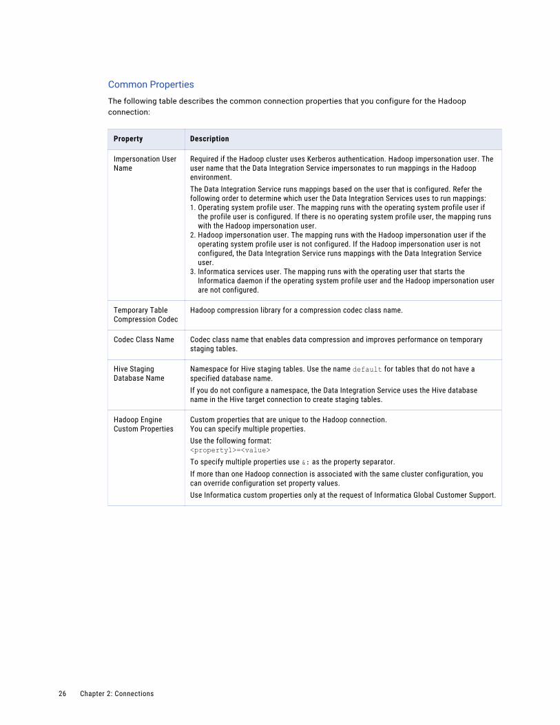
Common Properties
The following table describes the common connection properties that you configure for the Hadoop connection:
Property Description
Impersonation User Name
Required if the Hadoop cluster uses Kerberos authentication. Hadoop impersonation user. The user name that the Data Integration Service impersonates to run mappings in the Hadoop environment.The Data Integration Service runs mappings based on the user that is configured. Refer the following order to determine which user the Data Integration Services uses to run mappings:1. Operating system profile user. The mapping runs with the operating system profile user if
the profile user is configured. If there is no operating system profile user, the mapping runs with the Hadoop impersonation user.
2. Hadoop impersonation user. The mapping runs with the Hadoop impersonation user if the operating system profile user is not configured. If the Hadoop impersonation user is not configured, the Data Integration Service runs mappings with the Data Integration Service user.
3. Informatica services user. The mapping runs with the operating user that starts the Informatica daemon if the operating system profile user and the Hadoop impersonation user are not configured.
Temporary Table Compression Codec
Hadoop compression library for a compression codec class name.
Codec Class Name Codec class name that enables data compression and improves performance on temporary staging tables.
Hive Staging Database Name
Namespace for Hive staging tables. Use the name default for tables that do not have a specified database name.If you do not configure a namespace, the Data Integration Service uses the Hive database name in the Hive target connection to create staging tables.
Hadoop Engine Custom Properties
Custom properties that are unique to the Hadoop connection.You can specify multiple properties.Use the following format:<property1>=<value>To specify multiple properties use &: as the property separator.If more than one Hadoop connection is associated with the same cluster configuration, you can override configuration set property values.Use Informatica custom properties only at the request of Informatica Global Customer Support.
26 Chapter 2: Connections
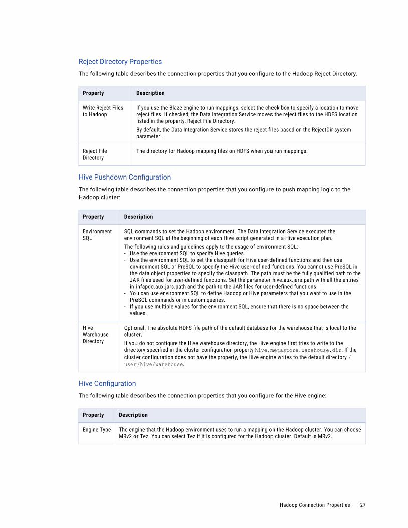
Reject Directory Properties
The following table describes the connection properties that you configure to the Hadoop Reject Directory.
Property Description
Write Reject Files to Hadoop
If you use the Blaze engine to run mappings, select the check box to specify a location to move reject files. If checked, the Data Integration Service moves the reject files to the HDFS location listed in the property, Reject File Directory.By default, the Data Integration Service stores the reject files based on the RejectDir system parameter.
Reject File Directory
The directory for Hadoop mapping files on HDFS when you run mappings.
Hive Pushdown Configuration
The following table describes the connection properties that you configure to push mapping logic to the Hadoop cluster:
Property Description
Environment SQL
SQL commands to set the Hadoop environment. The Data Integration Service executes the environment SQL at the beginning of each Hive script generated in a Hive execution plan.The following rules and guidelines apply to the usage of environment SQL:- Use the environment SQL to specify Hive queries.- Use the environment SQL to set the classpath for Hive user-defined functions and then use
environment SQL or PreSQL to specify the Hive user-defined functions. You cannot use PreSQL in the data object properties to specify the classpath. The path must be the fully qualified path to the JAR files used for user-defined functions. Set the parameter hive.aux.jars.path with all the entries in infapdo.aux.jars.path and the path to the JAR files for user-defined functions.
- You can use environment SQL to define Hadoop or Hive parameters that you want to use in the PreSQL commands or in custom queries.
- If you use multiple values for the environment SQL, ensure that there is no space between the values.
Hive Warehouse Directory
Optional. The absolute HDFS file path of the default database for the warehouse that is local to the cluster.If you do not configure the Hive warehouse directory, the Hive engine first tries to write to the directory specified in the cluster configuration property hive.metastore.warehouse.dir. If the cluster configuration does not have the property, the Hive engine writes to the default directory /user/hive/warehouse.
Hive Configuration
The following table describes the connection properties that you configure for the Hive engine:
Property Description
Engine Type The engine that the Hadoop environment uses to run a mapping on the Hadoop cluster. You can choose MRv2 or Tez. You can select Tez if it is configured for the Hadoop cluster. Default is MRv2.
Hadoop Connection Properties 27
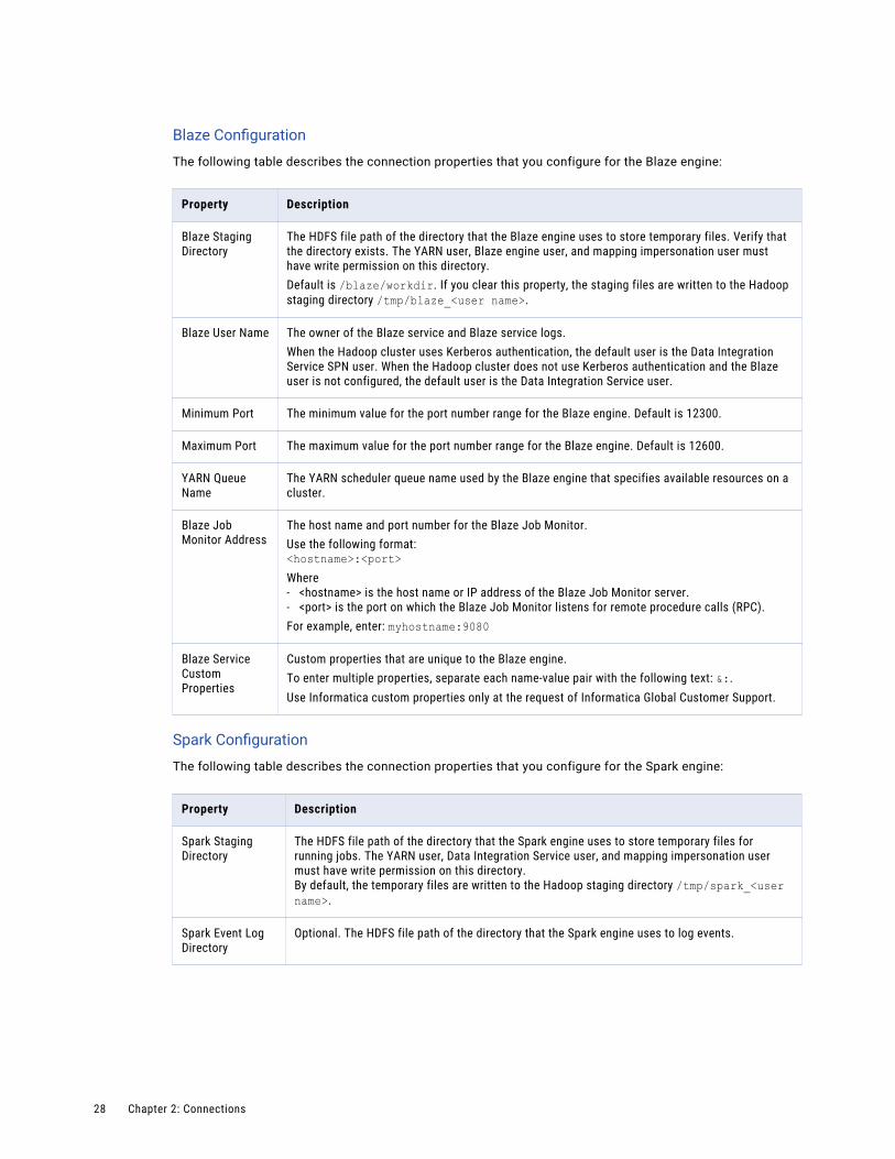
Blaze Configuration
The following table describes the connection properties that you configure for the Blaze engine:
Property Description
Blaze Staging Directory
The HDFS file path of the directory that the Blaze engine uses to store temporary files. Verify that the directory exists. The YARN user, Blaze engine user, and mapping impersonation user must have write permission on this directory.Default is /blaze/workdir. If you clear this property, the staging files are written to the Hadoop staging directory /tmp/blaze_<user name>.
Blaze User Name The owner of the Blaze service and Blaze service logs.When the Hadoop cluster uses Kerberos authentication, the default user is the Data Integration Service SPN user. When the Hadoop cluster does not use Kerberos authentication and the Blaze user is not configured, the default user is the Data Integration Service user.
Minimum Port The minimum value for the port number range for the Blaze engine. Default is 12300.
Maximum Port The maximum value for the port number range for the Blaze engine. Default is 12600.
YARN Queue Name
The YARN scheduler queue name used by the Blaze engine that specifies available resources on a cluster.
Blaze Job Monitor Address
The host name and port number for the Blaze Job Monitor.Use the following format:<hostname>:<port>Where- <hostname> is the host name or IP address of the Blaze Job Monitor server.- <port> is the port on which the Blaze Job Monitor listens for remote procedure calls (RPC).For example, enter: myhostname:9080
Blaze Service Custom Properties
Custom properties that are unique to the Blaze engine.To enter multiple properties, separate each name-value pair with the following text: &:.Use Informatica custom properties only at the request of Informatica Global Customer Support.
Spark Configuration
The following table describes the connection properties that you configure for the Spark engine:
Property Description
Spark Staging Directory
The HDFS file path of the directory that the Spark engine uses to store temporary files for running jobs. The YARN user, Data Integration Service user, and mapping impersonation user must have write permission on this directory.By default, the temporary files are written to the Hadoop staging directory /tmp/spark_<user name>.
Spark Event Log Directory
Optional. The HDFS file path of the directory that the Spark engine uses to log events.
28 Chapter 2: Connections
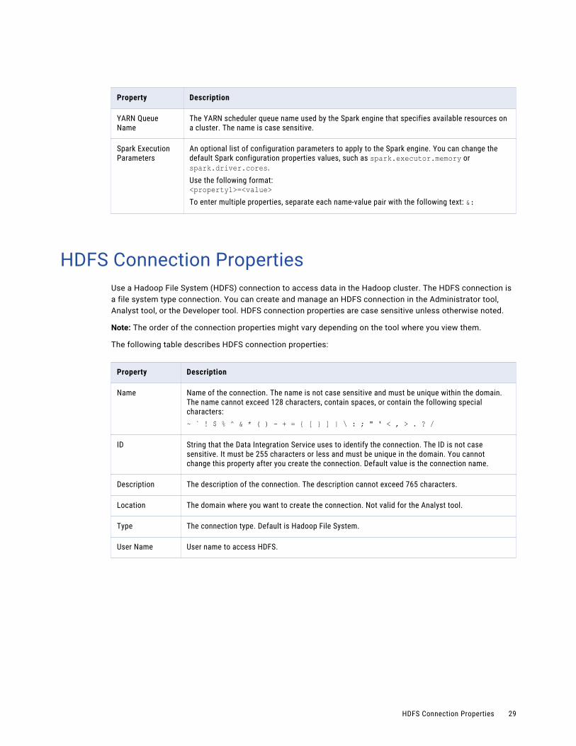
Property Description
YARN Queue Name
The YARN scheduler queue name used by the Spark engine that specifies available resources on a cluster. The name is case sensitive.
Spark Execution Parameters
An optional list of configuration parameters to apply to the Spark engine. You can change the default Spark configuration properties values, such as spark.executor.memory or spark.driver.cores.Use the following format:<property1>=<value>To enter multiple properties, separate each name-value pair with the following text: &:
HDFS Connection PropertiesUse a Hadoop File System (HDFS) connection to access data in the Hadoop cluster. The HDFS connection is a file system type connection. You can create and manage an HDFS connection in the Administrator tool, Analyst tool, or the Developer tool. HDFS connection properties are case sensitive unless otherwise noted.
Note: The order of the connection properties might vary depending on the tool where you view them.
The following table describes HDFS connection properties:
Property Description
Name Name of the connection. The name is not case sensitive and must be unique within the domain. The name cannot exceed 128 characters, contain spaces, or contain the following special characters:~ ` ! $ % ^ & * ( ) - + = { [ } ] | \ : ; " ' < , > . ? /
ID String that the Data Integration Service uses to identify the connection. The ID is not case sensitive. It must be 255 characters or less and must be unique in the domain. You cannot change this property after you create the connection. Default value is the connection name.
Description The description of the connection. The description cannot exceed 765 characters.
Location The domain where you want to create the connection. Not valid for the Analyst tool.
Type The connection type. Default is Hadoop File System.
User Name User name to access HDFS.
HDFS Connection Properties 29
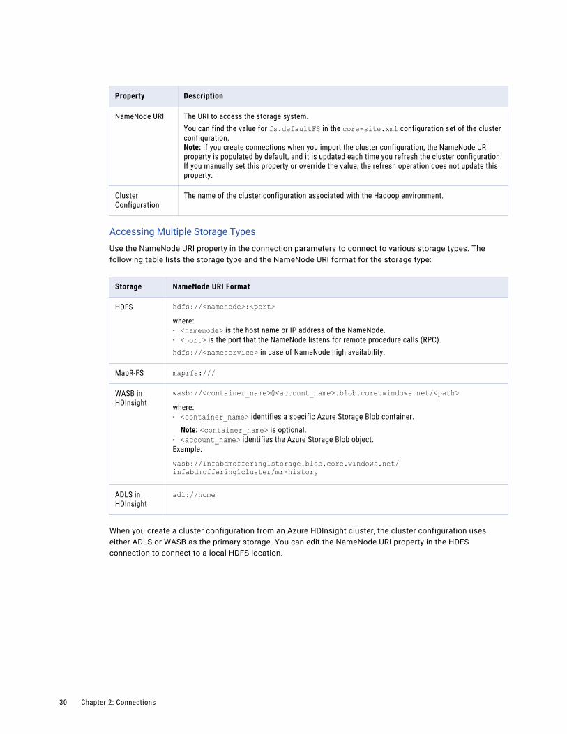
Property Description
NameNode URI The URI to access the storage system.You can find the value for fs.defaultFS in the core-site.xml configuration set of the cluster configuration.Note: If you create connections when you import the cluster configuration, the NameNode URI property is populated by default, and it is updated each time you refresh the cluster configuration. If you manually set this property or override the value, the refresh operation does not update this property.
Cluster Configuration
The name of the cluster configuration associated with the Hadoop environment.
Accessing Multiple Storage Types
Use the NameNode URI property in the connection parameters to connect to various storage types. The following table lists the storage type and the NameNode URI format for the storage type:
Storage NameNode URI Format
HDFS hdfs://<namenode>:<port>where:- <namenode> is the host name or IP address of the NameNode.- <port> is the port that the NameNode listens for remote procedure calls (RPC).hdfs://<nameservice> in case of NameNode high availability.
MapR-FS maprfs:///
WASB in HDInsight
wasb://<container_name>@<account_name>.blob.core.windows.net/<path>where:- <container_name> identifies a specific Azure Storage Blob container.
Note: <container_name> is optional.- <account_name> identifies the Azure Storage Blob object.Example:
wasb://infabdmoffering1storage.blob.core.windows.net/infabdmoffering1cluster/mr-history
ADLS in HDInsight
adl://home
When you create a cluster configuration from an Azure HDInsight cluster, the cluster configuration uses either ADLS or WASB as the primary storage. You can edit the NameNode URI property in the HDFS connection to connect to a local HDFS location.
30 Chapter 2: Connections

HBase Connection PropertiesUse an HBase connection to access HBase. The HBase connection is a NoSQL connection. You can create and manage an HBase connection in the Administrator tool or the Developer tool. HBase connection properties are case sensitive unless otherwise noted.
The following table describes HBase connection properties:
Property Description
Name The name of the connection. The name is not case sensitive and must be unique within the domain. You can change this property after you create the connection. The name cannot exceed 128 characters, contain spaces, or contain the following special characters:~ ` ! $ % ^ & * ( ) - + = { [ } ] | \ : ; " ' < , > . ? /
ID String that the Data Integration Service uses to identify the connection. The ID is not case sensitive. It must be 255 characters or less and must be unique in the domain. You cannot change this property after you create the connection. Default value is the connection name.
Description The description of the connection. The description cannot exceed 4,000 characters.
Location The domain where you want to create the connection.
Type The connection type. Select HBase.
Database Type Type of database that you want to connect to.Select HBase to create a connection for an HBase table.
Cluster Configuration The name of the cluster configuration associated with the Hadoop environment.
HBase Connection Properties 31
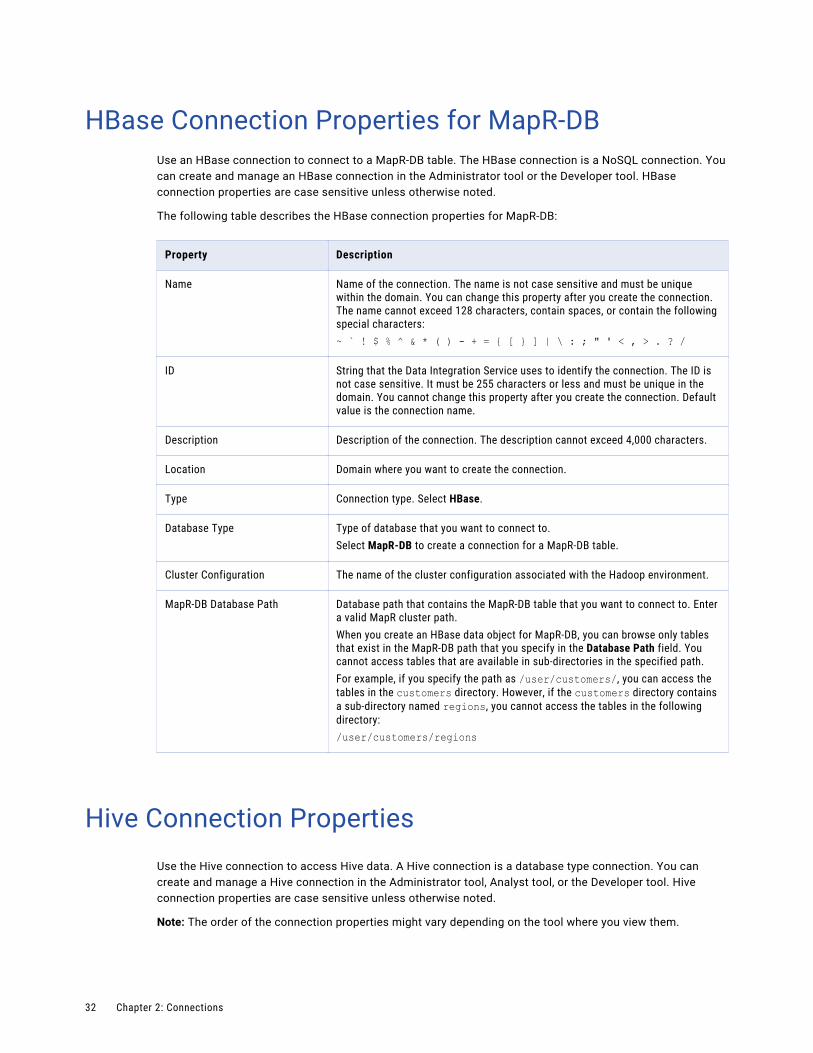
HBase Connection Properties for MapR-DBUse an HBase connection to connect to a MapR-DB table. The HBase connection is a NoSQL connection. You can create and manage an HBase connection in the Administrator tool or the Developer tool. HBase connection properties are case sensitive unless otherwise noted.
The following table describes the HBase connection properties for MapR-DB:
Property Description
Name Name of the connection. The name is not case sensitive and must be unique within the domain. You can change this property after you create the connection. The name cannot exceed 128 characters, contain spaces, or contain the following special characters:~ ` ! $ % ^ & * ( ) - + = { [ } ] | \ : ; " ' < , > . ? /
ID String that the Data Integration Service uses to identify the connection. The ID is not case sensitive. It must be 255 characters or less and must be unique in the domain. You cannot change this property after you create the connection. Default value is the connection name.
Description Description of the connection. The description cannot exceed 4,000 characters.
Location Domain where you want to create the connection.
Type Connection type. Select HBase.
Database Type Type of database that you want to connect to.Select MapR-DB to create a connection for a MapR-DB table.
Cluster Configuration The name of the cluster configuration associated with the Hadoop environment.
MapR-DB Database Path Database path that contains the MapR-DB table that you want to connect to. Enter a valid MapR cluster path.When you create an HBase data object for MapR-DB, you can browse only tables that exist in the MapR-DB path that you specify in the Database Path field. You cannot access tables that are available in sub-directories in the specified path.For example, if you specify the path as /user/customers/, you can access the tables in the customers directory. However, if the customers directory contains a sub-directory named regions, you cannot access the tables in the following directory:/user/customers/regions
Hive Connection PropertiesUse the Hive connection to access Hive data. A Hive connection is a database type connection. You can create and manage a Hive connection in the Administrator tool, Analyst tool, or the Developer tool. Hive connection properties are case sensitive unless otherwise noted.
Note: The order of the connection properties might vary depending on the tool where you view them.
32 Chapter 2: Connections
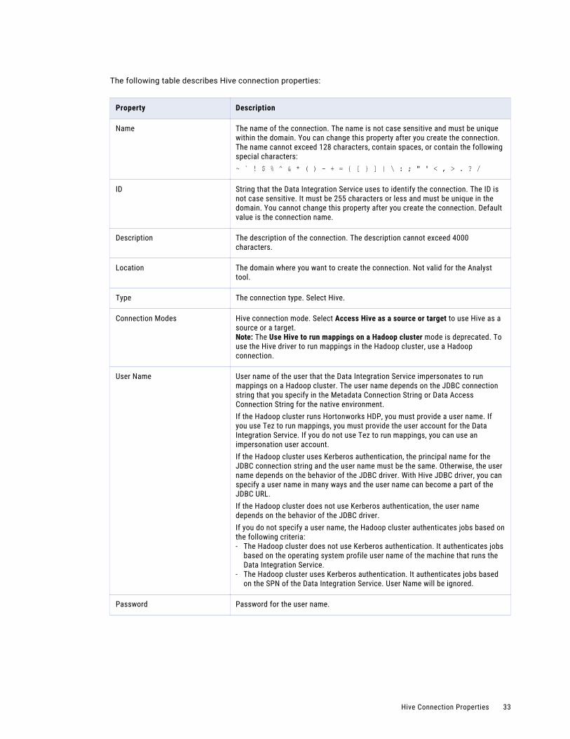
The following table describes Hive connection properties:
Property Description
Name The name of the connection. The name is not case sensitive and must be unique within the domain. You can change this property after you create the connection. The name cannot exceed 128 characters, contain spaces, or contain the following special characters:~ ` ! $ % ^ & * ( ) - + = { [ } ] | \ : ; " ' < , > . ? /
ID String that the Data Integration Service uses to identify the connection. The ID is not case sensitive. It must be 255 characters or less and must be unique in the domain. You cannot change this property after you create the connection. Default value is the connection name.
Description The description of the connection. The description cannot exceed 4000 characters.
Location The domain where you want to create the connection. Not valid for the Analyst tool.
Type The connection type. Select Hive.
Connection Modes Hive connection mode. Select Access Hive as a source or target to use Hive as a source or a target.Note: The Use Hive to run mappings on a Hadoop cluster mode is deprecated. To use the Hive driver to run mappings in the Hadoop cluster, use a Hadoop connection.
User Name User name of the user that the Data Integration Service impersonates to run mappings on a Hadoop cluster. The user name depends on the JDBC connection string that you specify in the Metadata Connection String or Data Access Connection String for the native environment.If the Hadoop cluster runs Hortonworks HDP, you must provide a user name. If you use Tez to run mappings, you must provide the user account for the Data Integration Service. If you do not use Tez to run mappings, you can use an impersonation user account.If the Hadoop cluster uses Kerberos authentication, the principal name for the JDBC connection string and the user name must be the same. Otherwise, the user name depends on the behavior of the JDBC driver. With Hive JDBC driver, you can specify a user name in many ways and the user name can become a part of the JDBC URL.If the Hadoop cluster does not use Kerberos authentication, the user name depends on the behavior of the JDBC driver.If you do not specify a user name, the Hadoop cluster authenticates jobs based on the following criteria:- The Hadoop cluster does not use Kerberos authentication. It authenticates jobs
based on the operating system profile user name of the machine that runs the Data Integration Service.
- The Hadoop cluster uses Kerberos authentication. It authenticates jobs based on the SPN of the Data Integration Service. User Name will be ignored.
Password Password for the user name.
Hive Connection Properties 33
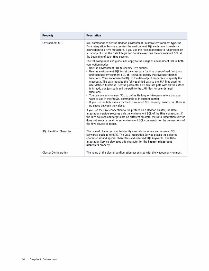
Property Description
Environment SQL SQL commands to set the Hadoop environment. In native environment type, the Data Integration Service executes the environment SQL each time it creates a connection to a Hive metastore. If you use the Hive connection to run profiles on a Hadoop cluster, the Data Integration Service executes the environment SQL at the beginning of each Hive session.The following rules and guidelines apply to the usage of environment SQL in both connection modes:- Use the environment SQL to specify Hive queries.- Use the environment SQL to set the classpath for Hive user-defined functions
and then use environment SQL or PreSQL to specify the Hive user-defined functions. You cannot use PreSQL in the data object properties to specify the classpath. The path must be the fully qualified path to the JAR files used for user-defined functions. Set the parameter hive.aux.jars.path with all the entries in infapdo.aux.jars.path and the path to the JAR files for user-defined functions.
- You can use environment SQL to define Hadoop or Hive parameters that you want to use in the PreSQL commands or in custom queries.
- If you use multiple values for the Environment SQL property, ensure that there is no space between the values.
If you use the Hive connection to run profiles on a Hadoop cluster, the Data Integration service executes only the environment SQL of the Hive connection. If the Hive sources and targets are on different clusters, the Data Integration Service does not execute the different environment SQL commands for the connections of the Hive source or target.
SQL Identifier Character The type of character used to identify special characters and reserved SQL keywords, such as WHERE. The Data Integration Service places the selected character around special characters and reserved SQL keywords. The Data Integration Service also uses this character for the Support mixed-case identifiers property.
Cluster Configuration The name of the cluster configuration associated with the Hadoop environment.
34 Chapter 2: Connections
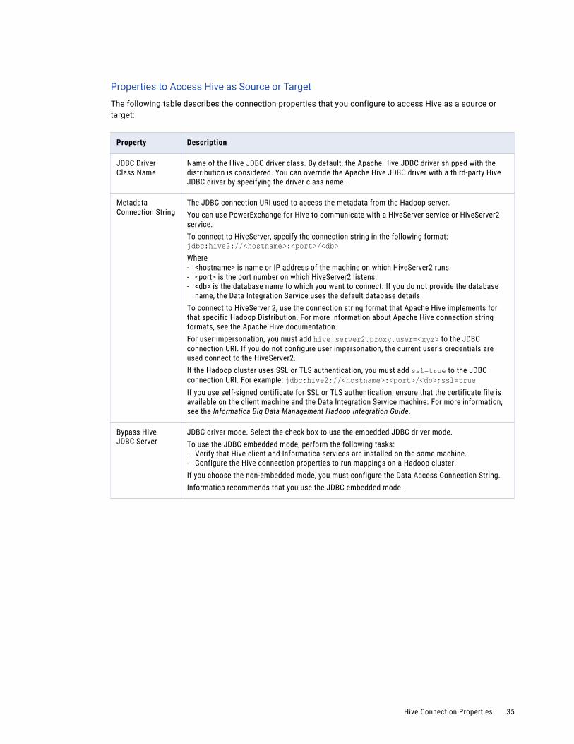
Properties to Access Hive as Source or Target
The following table describes the connection properties that you configure to access Hive as a source or target:
Property Description
JDBC Driver Class Name
Name of the Hive JDBC driver class. By default, the Apache Hive JDBC driver shipped with the distribution is considered. You can override the Apache Hive JDBC driver with a third-party Hive JDBC driver by specifying the driver class name.
Metadata Connection String
The JDBC connection URI used to access the metadata from the Hadoop server.You can use PowerExchange for Hive to communicate with a HiveServer service or HiveServer2 service.To connect to HiveServer, specify the connection string in the following format:jdbc:hive2://<hostname>:<port>/<db>Where- <hostname> is name or IP address of the machine on which HiveServer2 runs.- <port> is the port number on which HiveServer2 listens.- <db> is the database name to which you want to connect. If you do not provide the database
name, the Data Integration Service uses the default database details.To connect to HiveServer 2, use the connection string format that Apache Hive implements for that specific Hadoop Distribution. For more information about Apache Hive connection string formats, see the Apache Hive documentation.For user impersonation, you must add hive.server2.proxy.user=<xyz> to the JDBC connection URI. If you do not configure user impersonation, the current user's credentials are used connect to the HiveServer2.If the Hadoop cluster uses SSL or TLS authentication, you must add ssl=true to the JDBC connection URI. For example: jdbc:hive2://<hostname>:<port>/<db>;ssl=trueIf you use self-signed certificate for SSL or TLS authentication, ensure that the certificate file is available on the client machine and the Data Integration Service machine. For more information, see the Informatica Big Data Management Hadoop Integration Guide.
Bypass Hive JDBC Server
JDBC driver mode. Select the check box to use the embedded JDBC driver mode.To use the JDBC embedded mode, perform the following tasks:- Verify that Hive client and Informatica services are installed on the same machine.- Configure the Hive connection properties to run mappings on a Hadoop cluster.If you choose the non-embedded mode, you must configure the Data Access Connection String.Informatica recommends that you use the JDBC embedded mode.
Hive Connection Properties 35
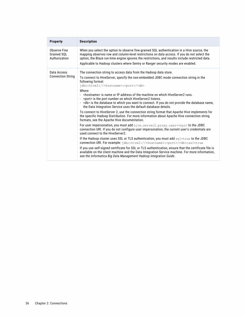
Property Description
Observe Fine Grained SQL Authorization
When you select the option to observe fine-grained SQL authentication in a Hive source, the mapping observes row and column-level restrictions on data access. If you do not select the option, the Blaze run-time engine ignores the restrictions, and results include restricted data.Applicable to Hadoop clusters where Sentry or Ranger security modes are enabled.
Data Access Connection String
The connection string to access data from the Hadoop data store.To connect to HiveServer, specify the non-embedded JDBC mode connection string in the following format:jdbc:hive2://<hostname>:<port>/<db>Where- <hostname> is name or IP address of the machine on which HiveServer2 runs.- <port> is the port number on which HiveServer2 listens.- <db> is the database to which you want to connect. If you do not provide the database name,
the Data Integration Service uses the default database details.To connect to HiveServer 2, use the connection string format that Apache Hive implements for the specific Hadoop Distribution. For more information about Apache Hive connection string formats, see the Apache Hive documentation.For user impersonation, you must add hive.server2.proxy.user=<xyz> to the JDBC connection URI. If you do not configure user impersonation, the current user's credentials are used connect to the HiveServer2.If the Hadoop cluster uses SSL or TLS authentication, you must add ssl=true to the JDBC connection URI. For example: jdbc:hive2://<hostname>:<port>/<db>;ssl=trueIf you use self-signed certificate for SSL or TLS authentication, ensure that the certificate file is available on the client machine and the Data Integration Service machine. For more information, see the Informatica Big Data Management Hadoop Integration Guide.
36 Chapter 2: Connections
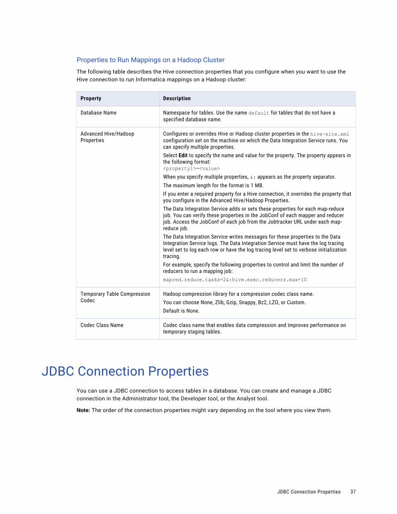
Properties to Run Mappings on a Hadoop Cluster
The following table describes the Hive connection properties that you configure when you want to use the Hive connection to run Informatica mappings on a Hadoop cluster:
Property Description
Database Name Namespace for tables. Use the name default for tables that do not have a specified database name.
Advanced Hive/Hadoop Properties
Configures or overrides Hive or Hadoop cluster properties in the hive-site.xml configuration set on the machine on which the Data Integration Service runs. You can specify multiple properties.Select Edit to specify the name and value for the property. The property appears in the following format:<property1>=<value>When you specify multiple properties, &: appears as the property separator.The maximum length for the format is 1 MB.If you enter a required property for a Hive connection, it overrides the property that you configure in the Advanced Hive/Hadoop Properties.The Data Integration Service adds or sets these properties for each map-reduce job. You can verify these properties in the JobConf of each mapper and reducer job. Access the JobConf of each job from the Jobtracker URL under each map-reduce job.The Data Integration Service writes messages for these properties to the Data Integration Service logs. The Data Integration Service must have the log tracing level set to log each row or have the log tracing level set to verbose initialization tracing.For example, specify the following properties to control and limit the number of reducers to run a mapping job:mapred.reduce.tasks=2&:hive.exec.reducers.max=10
Temporary Table Compression Codec
Hadoop compression library for a compression codec class name.You can choose None, Zlib, Gzip, Snappy, Bz2, LZO, or Custom.Default is None.
Codec Class Name Codec class name that enables data compression and improves performance on temporary staging tables.
JDBC Connection PropertiesYou can use a JDBC connection to access tables in a database. You can create and manage a JDBC connection in the Administrator tool, the Developer tool, or the Analyst tool.
Note: The order of the connection properties might vary depending on the tool where you view them.
JDBC Connection Properties 37
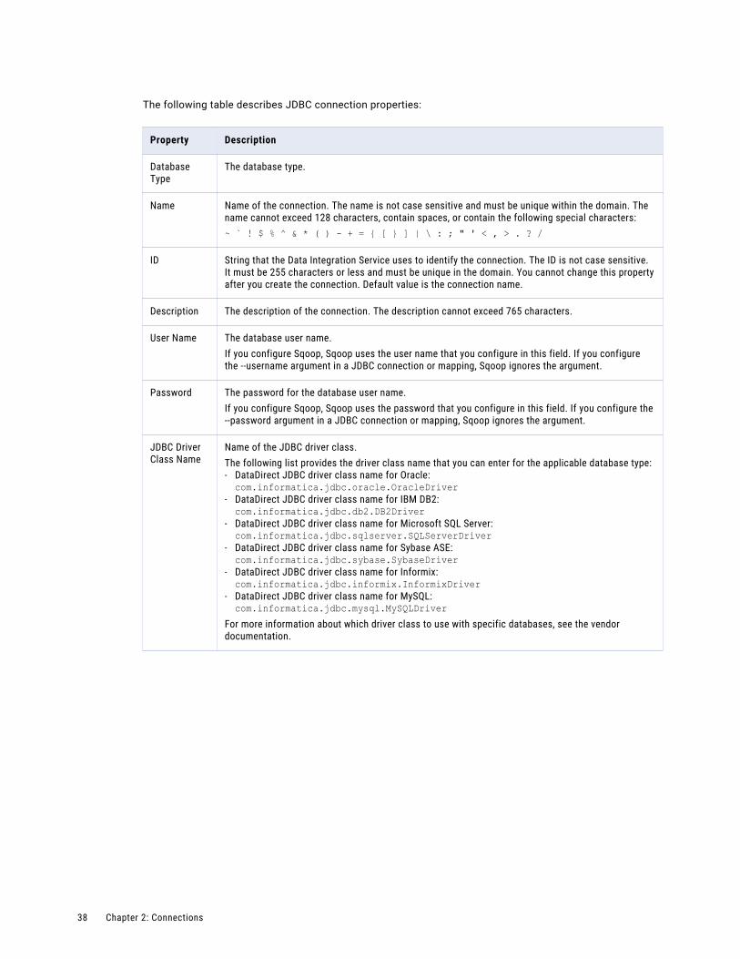
The following table describes JDBC connection properties:
Property Description
Database Type
The database type.
Name Name of the connection. The name is not case sensitive and must be unique within the domain. The name cannot exceed 128 characters, contain spaces, or contain the following special characters:~ ` ! $ % ^ & * ( ) - + = { [ } ] | \ : ; " ' < , > . ? /
ID String that the Data Integration Service uses to identify the connection. The ID is not case sensitive. It must be 255 characters or less and must be unique in the domain. You cannot change this property after you create the connection. Default value is the connection name.
Description The description of the connection. The description cannot exceed 765 characters.
User Name The database user name.If you configure Sqoop, Sqoop uses the user name that you configure in this field. If you configure the --username argument in a JDBC connection or mapping, Sqoop ignores the argument.
Password The password for the database user name.If you configure Sqoop, Sqoop uses the password that you configure in this field. If you configure the --password argument in a JDBC connection or mapping, Sqoop ignores the argument.
JDBC Driver Class Name
Name of the JDBC driver class.The following list provides the driver class name that you can enter for the applicable database type:- DataDirect JDBC driver class name for Oracle:com.informatica.jdbc.oracle.OracleDriver
- DataDirect JDBC driver class name for IBM DB2:com.informatica.jdbc.db2.DB2Driver
- DataDirect JDBC driver class name for Microsoft SQL Server:com.informatica.jdbc.sqlserver.SQLServerDriver
- DataDirect JDBC driver class name for Sybase ASE:com.informatica.jdbc.sybase.SybaseDriver
- DataDirect JDBC driver class name for Informix:com.informatica.jdbc.informix.InformixDriver
- DataDirect JDBC driver class name for MySQL:com.informatica.jdbc.mysql.MySQLDriver
For more information about which driver class to use with specific databases, see the vendor documentation.
38 Chapter 2: Connections
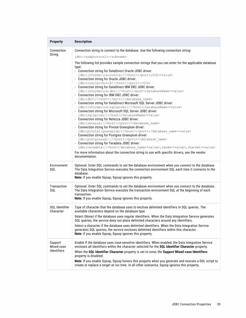
Property Description
Connection String
Connection string to connect to the database. Use the following connection string:
jdbc:<subprotocol>:<subname>The following list provides sample connection strings that you can enter for the applicable database type:- Connection string for DataDirect Oracle JDBC driver:jdbc:informatica:oracle://<host>:<port>;SID=<value>
- Connection string for Oracle JDBC driver:jdbc:oracle:thin:@//<host>:<port>:<SID>
- Connection string for DataDirect IBM DB2 JDBC driver:jdbc:informatica:db2://<host>:<port>;DatabaseName=<value>
- Connection string for IBM DB2 JDBC driver:jdbc:db2://<host>:<port>/<database_name>
- Connection string for DataDirect Microsoft SQL Server JDBC driver:jdbc:informatica:sqlserver://<host>;DatabaseName=<value>
- Connection string for Microsoft SQL Server JDBC driver:jdbc:sqlserver://<host>;DatabaseName=<value>
- Connection string for Netezza JDBC driver:jdbc:netezza://<host>:<port>/<database_name>
- Connection string for Pivotal Greenplum driver:jdbc:pivotal:greenplum://<host>:<port>;/database_name=<value>
- Connection string for Postgres Greenplum driver:jdbc:postgressql://<host>:<port>/<database_name>
- Connection string for Teradata JDBC driver:jdbc:teradata://<host>/database_name=<value>,tmode=<value>,charset=<value>
For more information about the connection string to use with specific drivers, see the vendor documentation.
Environment SQL
Optional. Enter SQL commands to set the database environment when you connect to the database. The Data Integration Service executes the connection environment SQL each time it connects to the database.Note: If you enable Sqoop, Sqoop ignores this property.
Transaction SQL
Optional. Enter SQL commands to set the database environment when you connect to the database. The Data Integration Service executes the transaction environment SQL at the beginning of each transaction.Note: If you enable Sqoop, Sqoop ignores this property.
SQL Identifier Character
Type of character that the database uses to enclose delimited identifiers in SQL queries. The available characters depend on the database type.Select (None) if the database uses regular identifiers. When the Data Integration Service generates SQL queries, the service does not place delimited characters around any identifiers.Select a character if the database uses delimited identifiers. When the Data Integration Service generates SQL queries, the service encloses delimited identifiers within this character.Note: If you enable Sqoop, Sqoop ignores this property.
Support Mixed-case Identifiers
Enable if the database uses case-sensitive identifiers. When enabled, the Data Integration Service encloses all identifiers within the character selected for the SQL Identifier Character property.When the SQL Identifier Character property is set to none, the Support Mixed-case Identifiers property is disabled.Note: If you enable Sqoop, Sqoop honors this property when you generate and execute a DDL script to create or replace a target at run time. In all other scenarios, Sqoop ignores this property.
JDBC Connection Properties 39
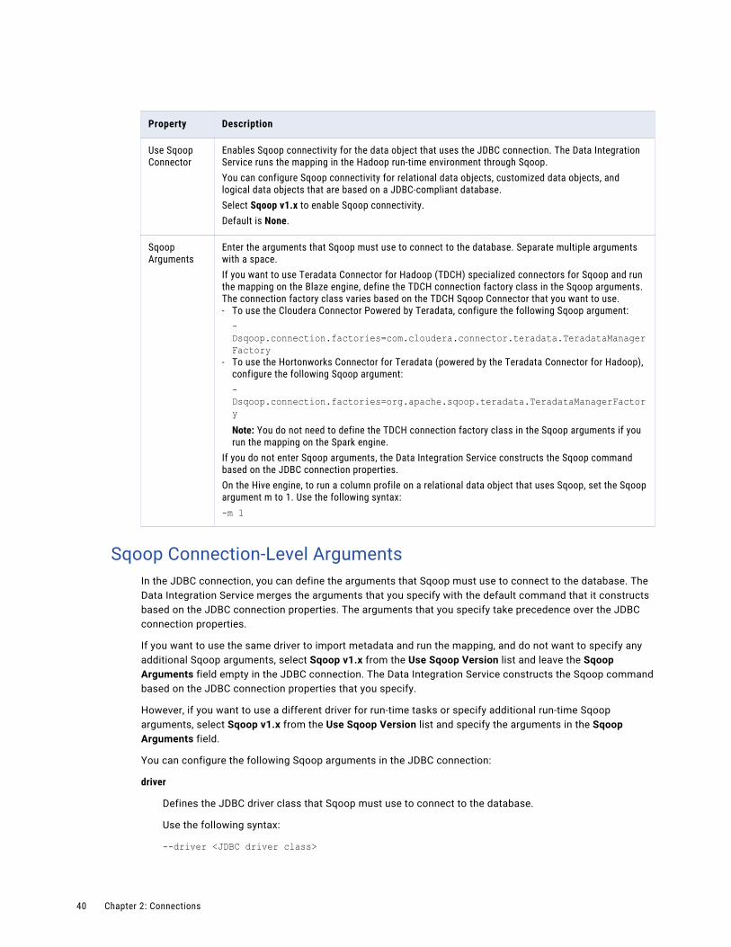
Property Description
Use Sqoop Connector
Enables Sqoop connectivity for the data object that uses the JDBC connection. The Data Integration Service runs the mapping in the Hadoop run-time environment through Sqoop.You can configure Sqoop connectivity for relational data objects, customized data objects, and logical data objects that are based on a JDBC-compliant database.Select Sqoop v1.x to enable Sqoop connectivity.Default is None.
Sqoop Arguments
Enter the arguments that Sqoop must use to connect to the database. Separate multiple arguments with a space.If you want to use Teradata Connector for Hadoop (TDCH) specialized connectors for Sqoop and run the mapping on the Blaze engine, define the TDCH connection factory class in the Sqoop arguments. The connection factory class varies based on the TDCH Sqoop Connector that you want to use.- To use the Cloudera Connector Powered by Teradata, configure the following Sqoop argument:-Dsqoop.connection.factories=com.cloudera.connector.teradata.TeradataManagerFactory
- To use the Hortonworks Connector for Teradata (powered by the Teradata Connector for Hadoop), configure the following Sqoop argument:-Dsqoop.connection.factories=org.apache.sqoop.teradata.TeradataManagerFactoryNote: You do not need to define the TDCH connection factory class in the Sqoop arguments if you run the mapping on the Spark engine.
If you do not enter Sqoop arguments, the Data Integration Service constructs the Sqoop command based on the JDBC connection properties.On the Hive engine, to run a column profile on a relational data object that uses Sqoop, set the Sqoop argument m to 1. Use the following syntax:-m 1
Sqoop Connection-Level ArgumentsIn the JDBC connection, you can define the arguments that Sqoop must use to connect to the database. The Data Integration Service merges the arguments that you specify with the default command that it constructs based on the JDBC connection properties. The arguments that you specify take precedence over the JDBC connection properties.
If you want to use the same driver to import metadata and run the mapping, and do not want to specify any additional Sqoop arguments, select Sqoop v1.x from the Use Sqoop Version list and leave the Sqoop Arguments field empty in the JDBC connection. The Data Integration Service constructs the Sqoop command based on the JDBC connection properties that you specify.
However, if you want to use a different driver for run-time tasks or specify additional run-time Sqoop arguments, select Sqoop v1.x from the Use Sqoop Version list and specify the arguments in the Sqoop Arguments field.
You can configure the following Sqoop arguments in the JDBC connection:
driver
Defines the JDBC driver class that Sqoop must use to connect to the database.
Use the following syntax:
--driver <JDBC driver class>
40 Chapter 2: Connections
For example, use the following syntax depending on the database type that you want to connect to:
• Aurora: --driver com.mysql.jdbc.Driver• Greenplum: --driver org.postgresql.Driver• IBM DB2: --driver com.ibm.db2.jcc.DB2Driver• IBM DB2 z/OS: --driver com.ibm.db2.jcc.DB2Driver• Microsoft SQL Server: --driver com.microsoft.sqlserver.jdbc.SQLServerDriver• Netezza: --driver org.netezza.Driver• Oracle: --driver oracle.jdbc.driver.OracleDriver• Teradata: --driver com.teradata.jdbc.TeraDriver
connect
Defines the JDBC connection string that Sqoop must use to connect to the database. The JDBC connection string must be based on the driver that you define in the driver argument.
Use the following syntax:
--connect <JDBC connection string>
For example, use the following syntax depending on the database type that you want to connect to:
• Aurora: --connect "jdbc:mysql://<host_name>:<port>/<schema_name>"• Greenplum: --connect jdbc:postgresql://<host_name>:<port>/<database_name>• IBM DB2: --connect jdbc:db2://<host_name>:<port>/<database_name>• IBM DB2 z/OS: --connect jdbc:db2://<host_name>:<port>/<database_name>• Microsoft SQL Server: --connect jdbc:sqlserver://<host_name>:<port or
named_instance>;databaseName=<database_name>• Netezza: --connect "jdbc:netezza://<database_server_name>:<port>/
<database_name>;schema=<schema_name>"• Oracle: --connect jdbc:oracle:thin:@<database_host_name>:<database_port>:<database_SID>• Teradata: --connect jdbc:teradata://<host_name>/database=<database_name>
direct
When you read data from or write data to Oracle, you can configure the direct argument to enable Sqoop to use OraOop. OraOop is a specialized Sqoop plug-in for Oracle that uses native protocols to connect to the Oracle database. When you configure OraOop, the performance improves.
You can configure OraOop when you run Sqoop mappings on the Spark and Hive engines.
Use the following syntax:
--direct
When you use OraOop, you must use the following syntax to specify multiple arguments:
-D<argument=value> -D<argument=value>
Note: If you specify multiple arguments and include a space character between -D and the argument name-value pair, Sqoop considers only the first argument and ignores the remaining arguments.
To direct a MapReduce job to a specific YARN queue, configure the following argument:
-Dmapred.job.queue.name=<YARN queue name>
JDBC Connection Properties 41
If you do not direct the job to a specific queue, the Spark engine uses the default queue.
-Dsqoop.connection.factories
If you want to use Teradata Connector for Hadoop (TDCH) specialized connectors for Sqoop and run the mapping on the Blaze engine, you can configure the -Dsqoop.connection.factories argument. Use the argument to define the TDCH connection factory class that Sqoop must use. The connection factory class varies based on the TDCH Sqoop Connector that you want to use.
• To use the Cloudera Connector Powered by Teradata, configure the -Dsqoop.connection.factories argument as follows:-Dsqoop.connection.factories=com.cloudera.connector.teradata.TeradataManagerFactory
• To use the Hortonworks Connector for Teradata (powered by the Teradata Connector for Hadoop), configure the -Dsqoop.connection.factories argument as follows:-Dsqoop.connection.factories=org.apache.sqoop.teradata.TeradataManagerFactory
Note: You do not need to configure the -Dsqoop.connection.factories argument if you run the mapping on the Spark engine.
For a complete list of the Sqoop arguments that you can configure, see the Sqoop documentation.
Creating a Connection to Access Sources or TargetsCreate an HBase, HDFS, Hive, or JDBC connection before you import data objects, preview data, and profile data.
1. Click Window > Preferences.
2. Select Informatica > Connections.
3. Expand the domain in the Available Connections list.
4. Select the type of connection that you want to create:
• To select an HBase connection, select NoSQL > HBase.
• To select an HDFS connection, select File Systems > Hadoop File System.
• To select a Hive connection, select Database > Hive.
• To select a JDBC connection, select Database > JDBC.
5. Click Add.
6. Enter a connection name and optional description.
7. Click Next.
8. Configure the connection properties. For a Hive connection, you must choose the Access Hive as a source or target option to use Hive as a source or a target. The Access Hive to run mappings in Hadoop cluster options is no more applicable. To use the Hive driver to run mappings in the Hadoop cluster, use a Hadoop connection.
9. Click Test Connection to verify the connection.
10. Click Finish.
42 Chapter 2: Connections
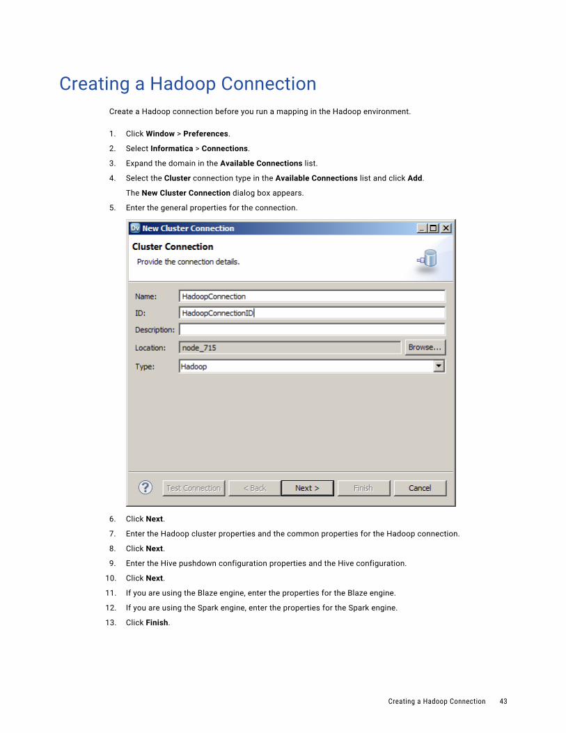
Creating a Hadoop ConnectionCreate a Hadoop connection before you run a mapping in the Hadoop environment.
1. Click Window > Preferences.
2. Select Informatica > Connections.
3. Expand the domain in the Available Connections list.
4. Select the Cluster connection type in the Available Connections list and click Add.
The New Cluster Connection dialog box appears.
5. Enter the general properties for the connection.
6. Click Next.
7. Enter the Hadoop cluster properties and the common properties for the Hadoop connection.
8. Click Next.
9. Enter the Hive pushdown configuration properties and the Hive configuration.
10. Click Next.
11. If you are using the Blaze engine, enter the properties for the Blaze engine.
12. If you are using the Spark engine, enter the properties for the Spark engine.
13. Click Finish.
Creating a Hadoop Connection 43

C h a p t e r 3
Mappings in the Hadoop Environment
This chapter includes the following topics:
• Mappings in the Hadoop Environment Overview, 44
• Mapping Run-time Properties, 45
• Data Warehouse Optimization Mapping Example , 48
• Sqoop Mappings in a Hadoop Environment, 50
• Rules and Guidelines for Mappings in a Hadoop Environment, 53
• Workflows that Run Mappings in a Hadoop Environment, 53
• Configuring a Mapping to Run in a Hadoop Environment, 54
• Mapping Execution Plans, 54
• Optimization for the Hadoop Environment, 57
• Troubleshooting a Mapping in a Hadoop Environment, 62
Mappings in the Hadoop Environment OverviewConfigure the Hadoop run-time environment in the Developer tool to optimize mapping performance and process data that is greater than 10 terabytes. In the Hadoop environment, the Data Integration Service pushes the processing to nodes on a Hadoop cluster. When you select the Hadoop environment, you can also select the engine to push the mapping logic to the Hadoop cluster.
You can run standalone mappings, mappings that are a part of a workflow in the Hadoop environment.
Based on the mapping logic, the Hadoop environment can use the following engines to push processing to nodes on a Hadoop cluster:
• Informatica Blaze engine. An Informatica proprietary engine for distributed processing on Hadoop.
• Spark engine. A high performance engine for batch processing that can run on a Hadoop cluster or on a Spark standalone mode cluster.
• Hive engine. A batch processing engine that uses Hadoop technology such as MapReduce or Tez.
When you configure the mapping, Informatica recommends that you select all engines. The Data Integration Service determines the best engine to run the mapping during validation. You can also choose to select which engine the Data Integration Service uses. You might select an engine based on whether an engine supports a particular transformation or based on the format in which the engine returns data.
44
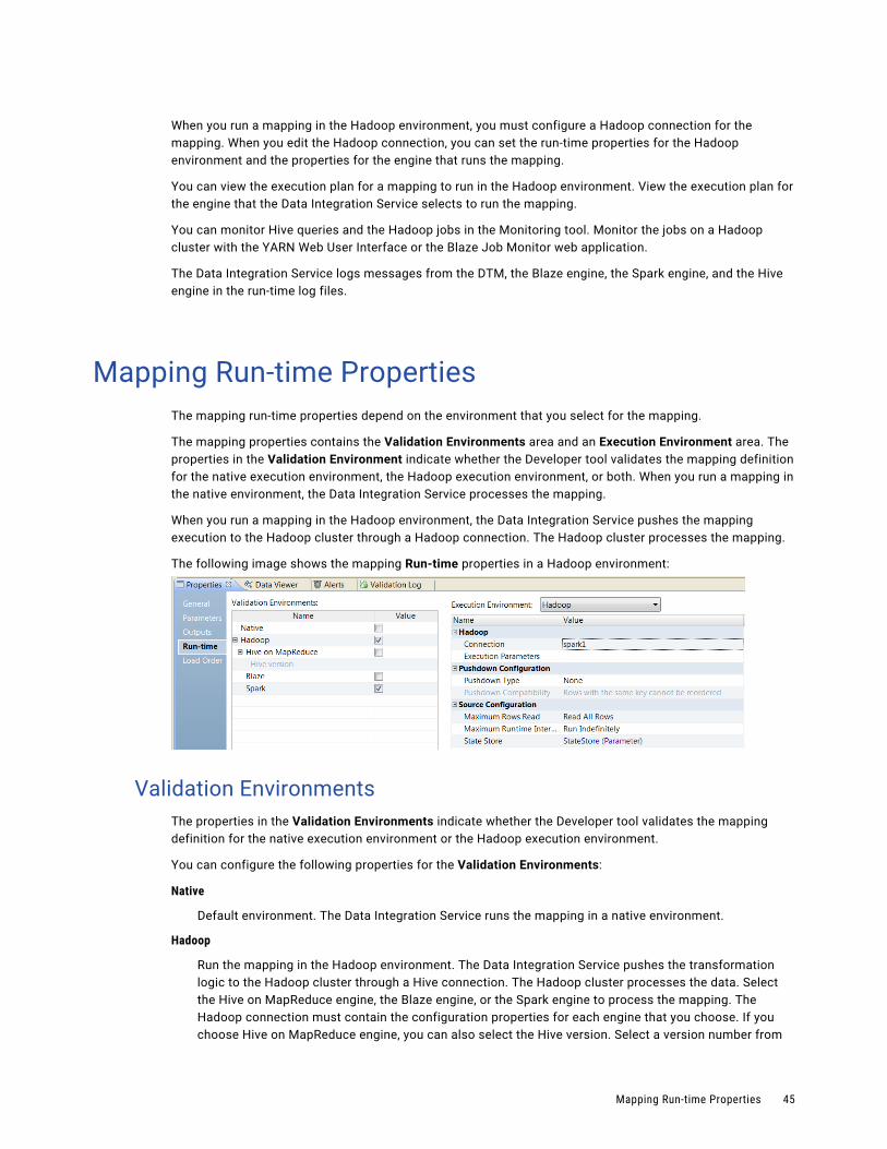
When you run a mapping in the Hadoop environment, you must configure a Hadoop connection for the mapping. When you edit the Hadoop connection, you can set the run-time properties for the Hadoop environment and the properties for the engine that runs the mapping.
You can view the execution plan for a mapping to run in the Hadoop environment. View the execution plan for the engine that the Data Integration Service selects to run the mapping.
You can monitor Hive queries and the Hadoop jobs in the Monitoring tool. Monitor the jobs on a Hadoop cluster with the YARN Web User Interface or the Blaze Job Monitor web application.
The Data Integration Service logs messages from the DTM, the Blaze engine, the Spark engine, and the Hive engine in the run-time log files.
Mapping Run-time PropertiesThe mapping run-time properties depend on the environment that you select for the mapping.
The mapping properties contains the Validation Environments area and an Execution Environment area. The properties in the Validation Environment indicate whether the Developer tool validates the mapping definition for the native execution environment, the Hadoop execution environment, or both. When you run a mapping in the native environment, the Data Integration Service processes the mapping.
When you run a mapping in the Hadoop environment, the Data Integration Service pushes the mapping execution to the Hadoop cluster through a Hadoop connection. The Hadoop cluster processes the mapping.
The following image shows the mapping Run-time properties in a Hadoop environment:
Validation EnvironmentsThe properties in the Validation Environments indicate whether the Developer tool validates the mapping definition for the native execution environment or the Hadoop execution environment.
You can configure the following properties for the Validation Environments:
Native
Default environment. The Data Integration Service runs the mapping in a native environment.
Hadoop
Run the mapping in the Hadoop environment. The Data Integration Service pushes the transformation logic to the Hadoop cluster through a Hive connection. The Hadoop cluster processes the data. Select the Hive on MapReduce engine, the Blaze engine, or the Spark engine to process the mapping. The Hadoop connection must contain the configuration properties for each engine that you choose. If you choose Hive on MapReduce engine, you can also select the Hive version. Select a version number from
Mapping Run-time Properties 45
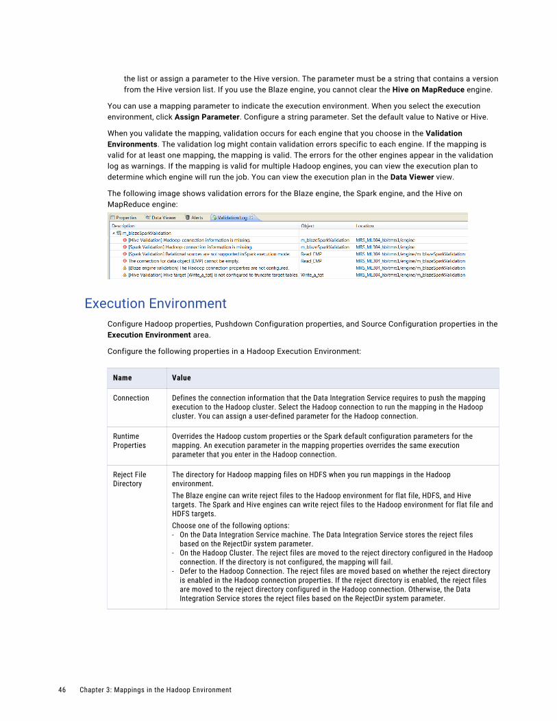
the list or assign a parameter to the Hive version. The parameter must be a string that contains a version from the Hive version list. If you use the Blaze engine, you cannot clear the Hive on MapReduce engine.
You can use a mapping parameter to indicate the execution environment. When you select the execution environment, click Assign Parameter. Configure a string parameter. Set the default value to Native or Hive.
When you validate the mapping, validation occurs for each engine that you choose in the Validation Environments. The validation log might contain validation errors specific to each engine. If the mapping is valid for at least one mapping, the mapping is valid. The errors for the other engines appear in the validation log as warnings. If the mapping is valid for multiple Hadoop engines, you can view the execution plan to determine which engine will run the job. You can view the execution plan in the Data Viewer view.
The following image shows validation errors for the Blaze engine, the Spark engine, and the Hive on MapReduce engine:
Execution EnvironmentConfigure Hadoop properties, Pushdown Configuration properties, and Source Configuration properties in the Execution Environment area.
Configure the following properties in a Hadoop Execution Environment:
Name Value
Connection Defines the connection information that the Data Integration Service requires to push the mapping execution to the Hadoop cluster. Select the Hadoop connection to run the mapping in the Hadoop cluster. You can assign a user-defined parameter for the Hadoop connection.
Runtime Properties
Overrides the Hadoop custom properties or the Spark default configuration parameters for the mapping. An execution parameter in the mapping properties overrides the same execution parameter that you enter in the Hadoop connection.
Reject File Directory
The directory for Hadoop mapping files on HDFS when you run mappings in the Hadoop environment.The Blaze engine can write reject files to the Hadoop environment for flat file, HDFS, and Hive targets. The Spark and Hive engines can write reject files to the Hadoop environment for flat file and HDFS targets.Choose one of the following options:- On the Data Integration Service machine. The Data Integration Service stores the reject files
based on the RejectDir system parameter.- On the Hadoop Cluster. The reject files are moved to the reject directory configured in the Hadoop
connection. If the directory is not configured, the mapping will fail.- Defer to the Hadoop Connection. The reject files are moved based on whether the reject directory
is enabled in the Hadoop connection properties. If the reject directory is enabled, the reject files are moved to the reject directory configured in the Hadoop connection. Otherwise, the Data Integration Service stores the reject files based on the RejectDir system parameter.
46 Chapter 3: Mappings in the Hadoop Environment
You can configure the following pushdown configuration properties:
Name Value
Pushdown type Choose one of the following options:- None. Select no pushdown type for the mapping.- Source. The Data Integration Service tries to push down transformation logic to the source
database.- Full. The Data Integration pushes the full transformation logic to the source database.
Pushdown Compatibility
Optionally, if you choose full pushdown optimization and the mapping contains an Update Strategy transformation, you can choose a pushdown compatibility option or assign a pushdown compatibility parameter.Choose one of the following options:- Multiple rows do not have the same key. The transformation connected to the Update Strategy
transformation receives multiple rows without the same key. The Data Integration Service can push the transformation logic to the target.
- Multiple rows with the same key can be reordered. The target transformation connected to the Update Strategy transformation receives multiple rows with the same key that can be reordered. The Data Integration Service can push the Update Strategy transformation to the Hadoop environment.
- Multiple rows with the same key cannot be reordered. The target transformation connected to the Update Strategy transformation receives multiple rows with the same key that cannot be reordered. The Data Integration Service cannot push the Update Strategy transformation to the Hadoop environment.
You can configure the following source properties:
Name Value
Maximum Rows Read Reserved for future use.
Maximum Runtime Interval Reserved for future use.
State Store Reserved for future use.
Reject File DirectoryYou can write reject files to the Data Integration Service machine or to the Hadoop cluster. Or, you can defer to the Hadoop connection configuration. The Blaze engine can write reject files to the Hadoop environment for flat file, HDFS, and Hive targets. The Spark and Hive engines can write reject files to the Hadoop environment for flat file and HDFS targets.
If you configure the mapping run-time properties to defer to the Hadoop connection, the reject files for all mappings with this configuration are moved based on whether you choose to write reject files to Hadoop for the active Hadoop connection. You do not need to change the mapping run-time properties manually to change the reject file directory.
For example, if the reject files are currently moved to the Data Integration Service machine and you want to move them to the directory configured in the Hadoop connection, edit the Hadoop connection properties to write reject files to Hadoop. The reject files of all mappings that are configured to defer to the Hadoop connection are moved to the configured directory.
You might also want to choose to defer to the Hadoop connection when the connection is parameterized to alternate between multiple Hadoop connections. For example, the parameter might alternate between one Hadoop connection that is configured to move reject files to the Data Integration Service machine and another Hadoop connection that is configured to move reject files to the directory configured in the Hadoop
Mapping Run-time Properties 47
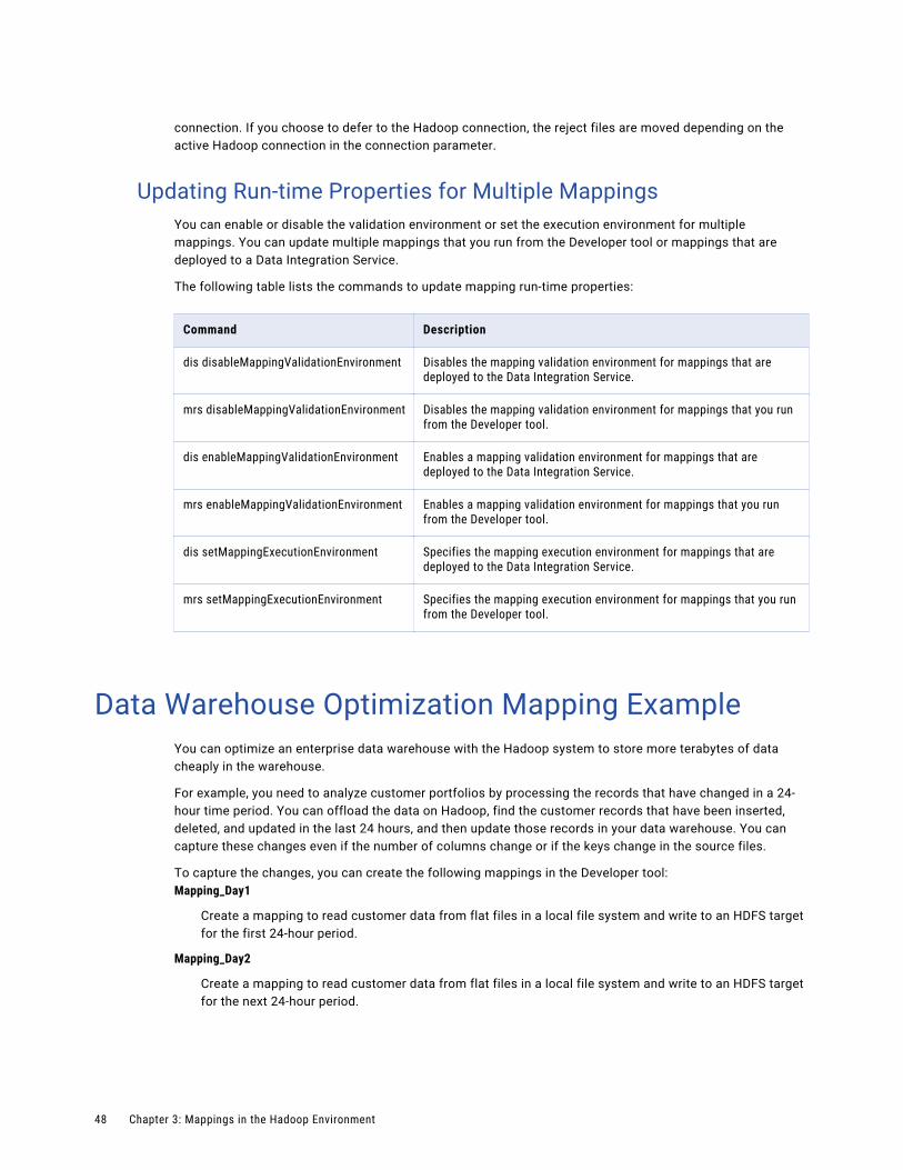
connection. If you choose to defer to the Hadoop connection, the reject files are moved depending on the active Hadoop connection in the connection parameter.
Updating Run-time Properties for Multiple MappingsYou can enable or disable the validation environment or set the execution environment for multiple mappings. You can update multiple mappings that you run from the Developer tool or mappings that are deployed to a Data Integration Service.
The following table lists the commands to update mapping run-time properties:
Command Description
dis disableMappingValidationEnvironment Disables the mapping validation environment for mappings that are deployed to the Data Integration Service.
mrs disableMappingValidationEnvironment Disables the mapping validation environment for mappings that you run from the Developer tool.
dis enableMappingValidationEnvironment Enables a mapping validation environment for mappings that are deployed to the Data Integration Service.
mrs enableMappingValidationEnvironment Enables a mapping validation environment for mappings that you run from the Developer tool.
dis setMappingExecutionEnvironment Specifies the mapping execution environment for mappings that are deployed to the Data Integration Service.
mrs setMappingExecutionEnvironment Specifies the mapping execution environment for mappings that you run from the Developer tool.
Data Warehouse Optimization Mapping ExampleYou can optimize an enterprise data warehouse with the Hadoop system to store more terabytes of data cheaply in the warehouse.
For example, you need to analyze customer portfolios by processing the records that have changed in a 24-hour time period. You can offload the data on Hadoop, find the customer records that have been inserted, deleted, and updated in the last 24 hours, and then update those records in your data warehouse. You can capture these changes even if the number of columns change or if the keys change in the source files.
To capture the changes, you can create the following mappings in the Developer tool:Mapping_Day1
Create a mapping to read customer data from flat files in a local file system and write to an HDFS target for the first 24-hour period.
Mapping_Day2
Create a mapping to read customer data from flat files in a local file system and write to an HDFS target for the next 24-hour period.
48 Chapter 3: Mappings in the Hadoop Environment
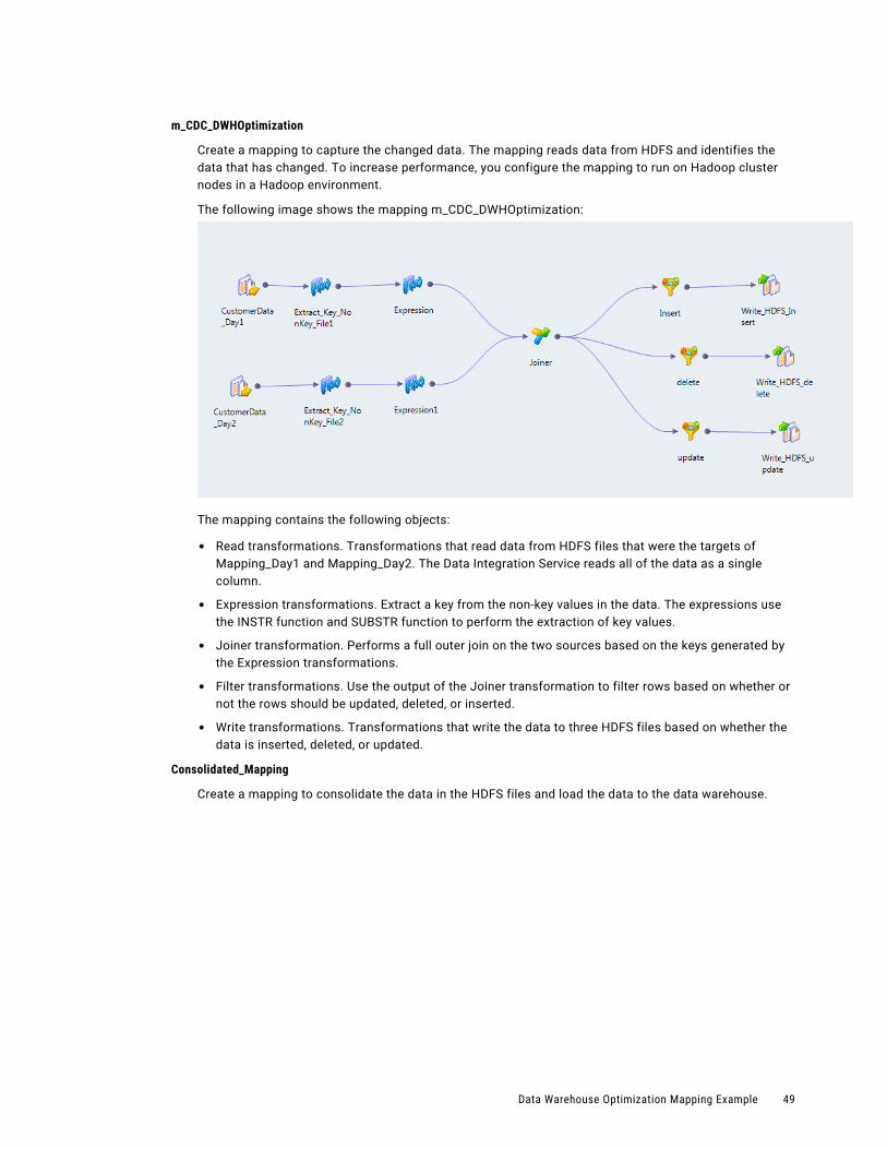
m_CDC_DWHOptimization
Create a mapping to capture the changed data. The mapping reads data from HDFS and identifies the data that has changed. To increase performance, you configure the mapping to run on Hadoop cluster nodes in a Hadoop environment.
The following image shows the mapping m_CDC_DWHOptimization:
The mapping contains the following objects:
• Read transformations. Transformations that read data from HDFS files that were the targets of Mapping_Day1 and Mapping_Day2. The Data Integration Service reads all of the data as a single column.
• Expression transformations. Extract a key from the non-key values in the data. The expressions use the INSTR function and SUBSTR function to perform the extraction of key values.
• Joiner transformation. Performs a full outer join on the two sources based on the keys generated by the Expression transformations.
• Filter transformations. Use the output of the Joiner transformation to filter rows based on whether or not the rows should be updated, deleted, or inserted.
• Write transformations. Transformations that write the data to three HDFS files based on whether the data is inserted, deleted, or updated.
Consolidated_Mapping
Create a mapping to consolidate the data in the HDFS files and load the data to the data warehouse.
Data Warehouse Optimization Mapping Example 49
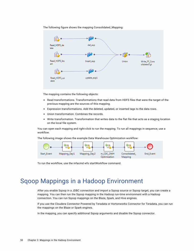
The following figure shows the mapping Consolidated_Mapping:
The mapping contains the following objects:
• Read transformations. Transformations that read data from HDFS files that were the target of the previous mapping are the sources of this mapping.
• Expression transformations. Add the deleted, updated, or inserted tags to the data rows.
• Union transformation. Combines the records.
• Write transformation. Transformation that writes data to the flat file that acts as a staging location on the local file system.
You can open each mapping and right-click to run the mapping. To run all mappings in sequence, use a workflow.
The following image shows the example Data Warehouse Optimization workflow:
To run the workflow, use the infacmd wfs startWorkflow command.
Sqoop Mappings in a Hadoop EnvironmentAfter you enable Sqoop in a JDBC connection and import a Sqoop source or Sqoop target, you can create a mapping. You can then run the Sqoop mapping in the Hadoop run-time environment with a Hadoop connection. You can run Sqoop mappings on the Blaze, Spark, and Hive engines.
If you use the Cloudera Connector Powered by Teradata or Hortonworks Connector for Teradata, you can run the mappings on the Blaze or Spark engines.
In the mapping, you can specify additional Sqoop arguments and disable the Sqoop connector.
50 Chapter 3: Mappings in the Hadoop Environment
Sqoop Mapping-Level ArgumentsIf a data object uses Sqoop, you can click the corresponding Read transformation or Write transformation in the Sqoop mapping to define the arguments that Sqoop must use to process the data. The Data Integration Service merges the additional Sqoop arguments that you specify in the mapping with the arguments that you specified in the JDBC connection and constructs the Sqoop command.
The Sqoop arguments that you specify in the mapping take precedence over the arguments that you specified in the JDBC connection. However, if you do not enable the Sqoop connector in the JDBC connection but enable the Sqoop connector in the mapping, the Data Integration Service does not run the mapping through Sqoop. The Data Integration Service runs the mapping through JDBC.
You can configure the following Sqoop arguments in a Sqoop mapping:
• m or num-mappers
• split-by
• batch
For a complete list of the Sqoop arguments that you can configure, see the Sqoop documentation.
m or num-mappersThe m or num-mappers argument defines the number of map tasks that Sqoop must use to import and export data in parallel.
Use the following syntax:
-m <number of map tasks>
--num-mappers <number of map tasks>
If you configure the m argument or num-mappers argument, you must also configure the split-by argument to specify the column based on which Sqoop must split the work units.
Use the m argument or num-mappers argument to increase the degree of parallelism. You might have to test different values for optimal performance.
When you configure the m argument or num-mappers argument and run Sqoop mappings on the Spark or Blaze engines, Sqoop dynamically creates partitions based on the file size.
Note: If you configure the num-mappers argument to export data on the Blaze or Spark engine, Sqoop ignores the argument. Sqoop creates map tasks based on the number of intermediate files that the Blaze or Spark engine creates.
split-byThe split-by argument defines the column based on which Sqoop splits work units.
Use the following syntax:
--split-by <column_name>
You can configure the split-by argument to improve the performance. If the primary key does not have an even distribution of values between the minimum and maximum range, you can configure the split-by argument to specify another column that has a balanced distribution of data to split the work units.
If you do not define the split-by column, Sqoop splits work units based on the following criteria:
• If the data object contains a single primary key, Sqoop uses the primary key as the split-by column.
Sqoop Mappings in a Hadoop Environment 51
• If the data object contains a composite primary key, Sqoop defaults to the behavior of handling composite primary keys without the split-by argument. See the Sqoop documentation for more information.
• If the data object does not contain a primary key, the value of the m argument and num-mappers argument default to 1.
Rules and Guidelines for the split-by Argument
Consider the following restrictions when you configure the split-by argument:
• If you configure the split-by argument and the split-by column contains NULL values, Sqoop does not import the rows that contain NULL values. However, the mapping runs successfully and no error is written in the YARN log.
• If you configure the split-by argument and the split-by column contains special characters, the Sqoop import process fails.
• The split-by argument is required in the following scenarios:
- You use the Cloudera Connector Powered by Teradata or Hortonworks Connector for Teradata, and the Teradata table does not contain a primary key.
- You create a custom query to override the default query when you import data from a Sqoop source.
batchThe batch argument indicates that Sqoop must export data in batches.
Use the following syntax:
--batch
You can configure the batch argument to improve the performance.
Configuring Sqoop Properties in the MappingYou can specify additional Sqoop arguments and disable the Sqoop connector at the mapping level. The Sqoop arguments that you specify at the mapping level take precedence over the arguments that you specified in the JDBC connection.
1. Open the mapping that contains the data object for which you want to configure Sqoop properties.
2. Select the Read or Write transformation that is associated with the data object.
3. Click the Advanced tab.
4. To disable the Sqoop connector for the data object, select the Disable Sqoop Connector check box.
5. Perform one of the following steps:
• To specify additional Sqoop import arguments for the data object, enter the import arguments in the Additional Sqoop Import Arguments text box.
• To specify additional Sqoop export arguments for the data object, enter the export arguments in the Additional Sqoop Export Arguments text box.
The Data Integration Service merges the additional Sqoop arguments that you specified in the mapping with the arguments that you specified in the JDBC connection and constructs the Sqoop command. The Data Integration Service then invokes Sqoop on a Hadoop node.
52 Chapter 3: Mappings in the Hadoop Environment
Rules and Guidelines for Mappings in a Hadoop Environment
You can run mappings in a Hadoop environment. When you run mappings in a Hadoop environment, some differences in processing and configuration apply.
The following processing differences apply to mappings in a Hadoop environment:
• A mapping is run in high precision mode in a Hadoop environment for Hive 0.11 and above.
• In a Hadoop environment, sources that have data errors in a column result in a null value for the column. In the native environment, the Data Integration Service does not process the rows that have data errors in a column.
• When you cancel a mapping that reads from a flat file source, the file copy process that copies flat file data to HDFS may continue to run. The Data Integration Service logs the command to kill this process in the Hive session log, and cleans up any data copied to HDFS. Optionally, you can run the command to kill the file copy process.
• When you set a limit on the number of rows read from the source for a Blaze mapping, the Data Integration Service runs the mapping with the Hive engine instead of the Blaze engine.
The following configuration differences apply to mappings in a Hadoop environment:
• Set the optimizer level to none or minimal if a mapping validates but fails to run. If you set the optimizer level to use cost-based or semi-join optimization methods, the Data Integration Service ignores this at run-time and uses the default.
• The Spark engine does not honor the early projection optimization method in all cases. If the Data Integration Service removes the links between unused ports, the Spark engine might reconnect the ports.
When the Spark engine runs a mapping, it processes jobs on the cluster using HiveServer2 in the following cases:
• The mapping writes to a target that is a Hive table bucketed on fields of type char or varchar.
• The mapping reads from or writes to Hive transaction-enabled tables.
• The mapping reads from or writes to Hive tables where column-level security is enabled.
• The mapping writes to a Hive target and is configured to create or replace the table at run time.
Workflows that Run Mappings in a Hadoop Environment
You can add a mapping that you configured to run in a Hadoop environment to a Mapping task in a workflow. When you deploy and run the workflow, the Mapping task runs the mapping.
You might decide to run a mapping from a workflow so that you can make decisions during the workflow run. You can configure a workflow to run multiple mappings in sequence or in parallel. You can configure a workflow to send emails that notify users about the status of the Mapping tasks.
When a Mapping task runs a mapping configured to run in a Hadoop environment, do not assign the Mapping task outputs to workflow variables. Mappings that run in a Hadoop environment do not provide the total number of target, source, and error rows. When a Mapping task includes a mapping that runs in a Hadoop environment, the task outputs contain a value of zero (0).
Rules and Guidelines for Mappings in a Hadoop Environment 53
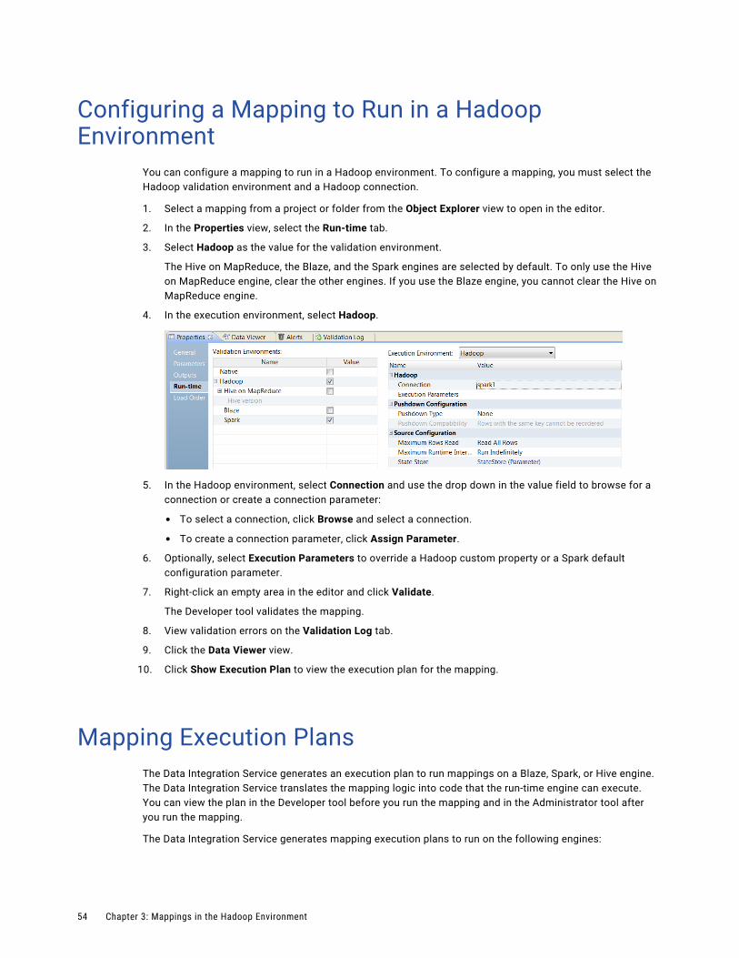
Configuring a Mapping to Run in a Hadoop Environment
You can configure a mapping to run in a Hadoop environment. To configure a mapping, you must select the Hadoop validation environment and a Hadoop connection.
1. Select a mapping from a project or folder from the Object Explorer view to open in the editor.
2. In the Properties view, select the Run-time tab.
3. Select Hadoop as the value for the validation environment.
The Hive on MapReduce, the Blaze, and the Spark engines are selected by default. To only use the Hive on MapReduce engine, clear the other engines. If you use the Blaze engine, you cannot clear the Hive on MapReduce engine.
4. In the execution environment, select Hadoop.
5. In the Hadoop environment, select Connection and use the drop down in the value field to browse for a connection or create a connection parameter:
• To select a connection, click Browse and select a connection.
• To create a connection parameter, click Assign Parameter.
6. Optionally, select Execution Parameters to override a Hadoop custom property or a Spark default configuration parameter.
7. Right-click an empty area in the editor and click Validate.
The Developer tool validates the mapping.
8. View validation errors on the Validation Log tab.
9. Click the Data Viewer view.
10. Click Show Execution Plan to view the execution plan for the mapping.
Mapping Execution PlansThe Data Integration Service generates an execution plan to run mappings on a Blaze, Spark, or Hive engine. The Data Integration Service translates the mapping logic into code that the run-time engine can execute. You can view the plan in the Developer tool before you run the mapping and in the Administrator tool after you run the mapping.
The Data Integration Service generates mapping execution plans to run on the following engines:
54 Chapter 3: Mappings in the Hadoop Environment

Informatica Blaze engine
The Blaze engine execution plan simplifies the mapping into segments. It contains tasks to start the mapping, run the mapping, and clean up the temporary tables and files. It contains multiple tasklets and the task recovery strategy. It also contains pre- and post-grid task preparation commands for each mapping before running the main mapping on a Hadoop cluster. A pre-grid task can include a task such as copying data to HDFS. A post-grid task can include tasks such as cleaning up temporary files or copying data from HDFS.
Spark engine
The Spark execution plan shows the run-time Scala code that runs the mapping logic. A translation engine translates the mapping into an internal representation of the logic. The internal representation is rendered into Scala code that accesses the Spark API. You can view the Scala code in the execution plan to debug the logic.
Hive engine
The Hive execution plan is a series of Hive queries. The plan contains tasks to start the mapping, run the mapping, and clean up the temporary tables and files. You can view the Hive execution plan that the Data Integration Service generates before you run the mapping. When the Data Integration Service pushes the mapping to the Hive engine, it has a Hive executor that can process the mapping. The Hive executor simplifies the mapping to an equivalent mapping with a reduced set of instructions and generates a Hive execution plan.
Blaze Engine Execution Plan DetailsYou can view details of the Blaze engine execution plan in the Administrator tool and Developer tool.
In the Developer tool, the Blaze engine execution plan appears as a workflow. You can click on each component in the workflow to get the details.
The following image shows the Blaze execution plan in the Developer tool:
The Blaze engine execution plan workflow contains the following components:
• Start task. The workflow start task.
Mapping Execution Plans 55
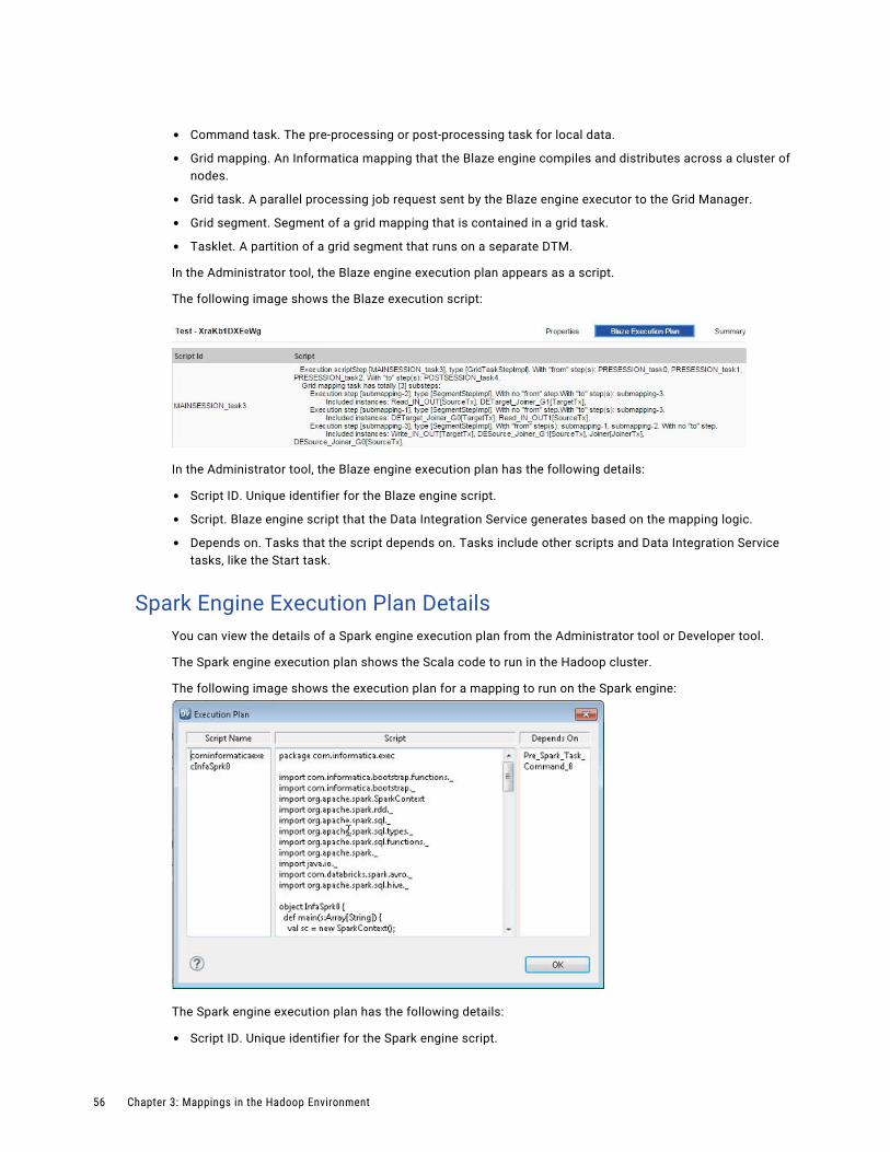
• Command task. The pre-processing or post-processing task for local data.
• Grid mapping. An Informatica mapping that the Blaze engine compiles and distributes across a cluster of nodes.
• Grid task. A parallel processing job request sent by the Blaze engine executor to the Grid Manager.
• Grid segment. Segment of a grid mapping that is contained in a grid task.
• Tasklet. A partition of a grid segment that runs on a separate DTM.
In the Administrator tool, the Blaze engine execution plan appears as a script.
The following image shows the Blaze execution script:
In the Administrator tool, the Blaze engine execution plan has the following details:
• Script ID. Unique identifier for the Blaze engine script.
• Script. Blaze engine script that the Data Integration Service generates based on the mapping logic.
• Depends on. Tasks that the script depends on. Tasks include other scripts and Data Integration Service tasks, like the Start task.
Spark Engine Execution Plan DetailsYou can view the details of a Spark engine execution plan from the Administrator tool or Developer tool.
The Spark engine execution plan shows the Scala code to run in the Hadoop cluster.
The following image shows the execution plan for a mapping to run on the Spark engine:
The Spark engine execution plan has the following details:
• Script ID. Unique identifier for the Spark engine script.
56 Chapter 3: Mappings in the Hadoop Environment
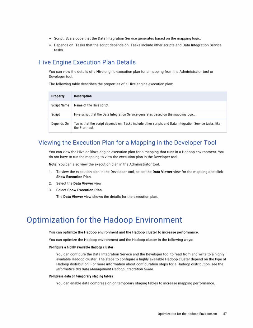
• Script. Scala code that the Data Integration Service generates based on the mapping logic.
• Depends on. Tasks that the script depends on. Tasks include other scripts and Data Integration Service tasks.
Hive Engine Execution Plan DetailsYou can view the details of a Hive engine execution plan for a mapping from the Administrator tool or Developer tool.
The following table describes the properties of a Hive engine execution plan:
Property Description
Script Name Name of the Hive script.
Script Hive script that the Data Integration Service generates based on the mapping logic.
Depends On Tasks that the script depends on. Tasks include other scripts and Data Integration Service tasks, like the Start task.
Viewing the Execution Plan for a Mapping in the Developer ToolYou can view the Hive or Blaze engine execution plan for a mapping that runs in a Hadoop environment. You do not have to run the mapping to view the execution plan in the Developer tool.
Note: You can also view the execution plan in the Administrator tool.
1. To view the execution plan in the Developer tool, select the Data Viewer view for the mapping and click Show Execution Plan.
2. Select the Data Viewer view.
3. Select Show Execution Plan.
The Data Viewer view shows the details for the execution plan.
Optimization for the Hadoop EnvironmentYou can optimize the Hadoop environment and the Hadoop cluster to increase performance.
You can optimize the Hadoop environment and the Hadoop cluster in the following ways:
Configure a highly available Hadoop cluster
You can configure the Data Integration Service and the Developer tool to read from and write to a highly available Hadoop cluster. The steps to configure a highly available Hadoop cluster depend on the type of Hadoop distribution. For more information about configuration steps for a Hadoop distribution, see the Informatica Big Data Management Hadoop Integration Guide.
Compress data on temporary staging tables
You can enable data compression on temporary staging tables to increase mapping performance.
Optimization for the Hadoop Environment 57
Run mappings on the Blaze engine
Run mappings on the highly available Blaze engine. The Blaze engine enables restart and recovery of grid tasks and tasklets by default.
Perform parallel sorts
When you use a Sorter transformation in a mapping, the Data Integration Service enables parallel sorting by default when it pushes the mapping logic to the Hadoop cluster. Parallel sorting improves mapping performance with some restrictions.
Partition Joiner transformations
When you use a Joiner transformation in a Blaze engine mapping, the Data Integration Service can apply map-side join optimization to improve mapping performance. The Data Integration Service applies map-side join optimization if the master table is smaller than the detail table. When the Data Integration Service applies map-side join optimization, it moves the data to the Joiner transformation without the cost of shuffling the data.
Truncate partitions in a Hive target
You can truncate partitions in a Hive target to increase performance. To truncate partitions in a Hive target, you must choose to both truncate the partition in the Hive target and truncate the target table. You can enable data compression on temporary staging tables to optimize performance.
Blaze Engine High AvailabilityThe Blaze engine is a highly available engine that determines the best possible recovery strategy for grid tasks and tasklets.
Based on the size of the grid task, the Blaze engine attempts to apply the following recovery strategy:
• No high availability. The Blaze engine not apply a recovery strategy.
• Full restart. Restarts the grid task.
Enabling Data Compression on Temporary Staging TablesTo optimize performance when you run a mapping in the Hadoop environment, you can enable data compression on temporary staging tables. When you enable data compression on temporary staging tables, mapping performance might increase.
To enable data compression on temporary staging tables, complete the following steps:
1. Configure the Hive connection to use the codec class name that the Hadoop cluster uses to enable compression on temporary staging tables.
2. Configure the Hadoop cluster to enable compression on temporary staging tables.
Hadoop provides following compression libraries for the following compression codec class names:
Compression Library Codec Class Name Performance Recommendation
Zlib org.apache.hadoop.io.compress.DefaultCodec n/a
Gzip org.apache.hadoop.io.compress.GzipCodec n/a
Snappy org.apache.hadoop.io.compress.SnappyCodec Recommended for best performance.
58 Chapter 3: Mappings in the Hadoop Environment
Compression Library Codec Class Name Performance Recommendation
Bz2 org.apache.hadoop.io.compress.BZip2Codec Not recommended. Degrades performance.
LZO com.hadoop.compression.lzo.LzoCodec n/a
Step 1. Configure the Hive Connection to Enable Data Compression on Temporary Staging TablesUse the Administrator tool or the Developer tool to configure the Hive connection. You can edit the Hive connection properties to configure the codec class name that enables data compression on temporary staging tables.
1. In the Hive connection properties, edit the properties to run mappings in a Hadoop cluster.
2. Select Temporary Table Compression Codec.
3. Choose to select a predefined codec class name or enter a custom codec class name.
• To select a predefined codec class name, select a compression library from the list.
• To enter a custom codec class name, select custom from the list and enter the codec class name that matches the codec class name in the Hadoop cluster.
Step 2. Configure the Hadoop Cluster to Enable Compression on Temporary Staging TablesTo enable compression on temporary staging tables, you must install a compression codec on the Hadoop cluster.
For more information about how to install a compression codec, refer to the Apache Hadoop or Hive documentation.
1. Verify that the native libraries for the compression codec class name are installed on every node on the cluster.
2. To include the compression codec class name that you want to use, update the property io.compression.codecs in core-site.xml. The value for this property is a comma separated list of all the codec class names supported on the cluster.
3. Verify that the Hadoop-native libraries for the compression codec class name that you want to use are installed on every node on the cluster.
4. Verify that the LD_LIBRARY_PATH variable on the Hadoop cluster includes the locations of both the native and Hadoop-native libraries where you installed the compression codec.
Parallel SortingTo improve mapping performance, the Data Integration Service enables parallel sorting by default in a mapping that has a Sorter transformation and a flat file target.
The Data Integration Service enables parallel sorting for mappings in a Hadoop environment based on the following rules and guidelines:
• The mapping does not include another transformation between the Sorter transformation and the target.
• The data type of the sort keys does not change between the Sorter transformation and the target.
• Each sort key in the Sorter transformation must be linked to a column in the target.
Optimization for the Hadoop Environment 59
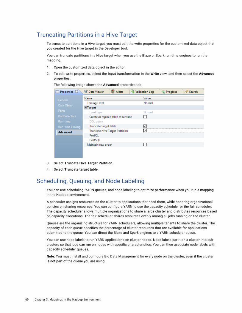
Truncating Partitions in a Hive TargetTo truncate partitions in a Hive target, you must edit the write properties for the customized data object that you created for the Hive target in the Developer tool.
You can truncate partitions in a Hive target when you use the Blaze or Spark run-time engines to run the mapping.
1. Open the customized data object in the editor.
2. To edit write properties, select the Input transformation in the Write view, and then select the Advanced properties.
The following image shows the Advanced properties tab:
3. Select Truncate Hive Target Partition.
4. Select Truncate target table.
Scheduling, Queuing, and Node LabelingYou can use scheduling, YARN queues, and node labeling to optimize performance when you run a mapping in the Hadoop environment.
A scheduler assigns resources on the cluster to applications that need them, while honoring organizational policies on sharing resources. You can configure YARN to use the capacity scheduler or the fair scheduler. The capacity scheduler allows multiple organizations to share a large cluster and distributes resources based on capacity allocations. The fair scheduler shares resources evenly among all jobs running on the cluster.
Queues are the organizing structure for YARN schedulers, allowing multiple tenants to share the cluster. The capacity of each queue specifies the percentage of cluster resources that are available for applications submitted to the queue. You can direct the Blaze and Spark engines to a YARN scheduler queue.
You can use node labels to run YARN applications on cluster nodes. Node labels partition a cluster into sub-clusters so that jobs can run on nodes with specific characteristics. You can then associate node labels with capacity scheduler queues.
Note: You must install and configure Big Data Management for every node on the cluster, even if the cluster is not part of the queue you are using.
60 Chapter 3: Mappings in the Hadoop Environment
Scheduling and Node Labeling ConfigurationUpdate the yarn-site.xml file on the domain environment to enable scheduling and node labeling in the Hadoop environment. Configure the following properties:
yarn.resourcemanager.scheduler.class
Defines the YARN scheduler that the Data Integration Service uses to assign resources on the cluster.
<property> <name>yarn.resourcemanager.scheduler.class</name> <value><org.apache.hadoop.yarn.server.resourcemanager.scheduler.[Scheduler Type].[Scheduler Type]Scheduler></value></property>
For example:
<property> <name>yarn.resourcemanager.scheduler.class</name> <value><org.apache.hadoop.yarn.server.resourcemanager.scheduler.capacity.CapacityScheduler></value></property>
yarn.node-labels.enabled
Enables node labeling.
<property> <name>yarn.node-labels.enabled</name> <value><TRUE></value></property>
yarn.node-labels.fs-store.root-dir
The HDFS location to update the node label dynamically.
<property> <name>yarn.node-labels.fs-store.root-dir</name> <value><hdfs://[Node name]:[Port]/[Path to store]/[Node labels]/></value></property>
Queuing Configuration
The following table describes the Hadoop connection property you configure to direct a job to a specific YARN scheduler queue:
Property Description
YARN Queue Name The connection property to specify a YARN scheduler queue name. Configure this property for the Blaze engine and the Spark engine. The name is case sensitive.
Optimization for the Hadoop Environment 61
The following table describes the Hive connection property you configure to direct a job to a specific YARN scheduler queue:
Property Description
Data Access Connection String
The Hive connection string to specify the queue name for Hive SQL override mappings on the Blaze engine.Use the following format:- MapReduce. mapred.job.queue.name=<YARN queue name>- Tez. tez.queue.name=<YARN queue name>For example, jdbc:hive2://business.com:10000/default;principal=hive/_HOST@INFAKRB?mapred.job.queue.name-root.test
The following table describes the JDBC connection property you configure to direct a job to a specific YARN scheduler queue:
Property Description
Sqoop Arguments The Sqoop connection-level argument to direct a MapReduce job to a specific YARN queue.Use the following format:-Dmapred.job.queue.name=<YARN queue name>If you do not direct the job to a specific queue, the Spark engine uses the default queue.
Troubleshooting a Mapping in a Hadoop EnvironmentWhen I run a mapping with a Hive source or a Hive target on a different cluster, the Data Integration Service fails to push the mapping to Hadoop with the following error: Failed to execute query [exec0_query_6] with error code [10], error message [FAILED: Error in semantic analysis: Line 1:181 Table not found customer_eur], and SQL state [42000]].
When you run a mapping in a Hadoop environment, the Hive connection selected for the Hive source or Hive target, and the mapping must be on the same Hive metastore.
When I run a mapping with a Hadoop distribution on MapReduce 2, the Administrator tool shows the percentage of completed reduce tasks as 0% instead of 100%.
Verify that the Hadoop jobs have reduce tasks.
When the Hadoop distribution is on MapReduce 2 and the Hadoop jobs do not contain reducer tasks, the Administrator tool shows the percentage of completed reduce tasks as 0%.
When the Hadoop distribution is on MapReduce 2 and the Hadoop jobs contain reducer tasks, the Administrator tool shows the percentage of completed reduce tasks as 100%.
When I run mappings with SQL overrides concurrently, the mappings hang.
There are not enough available resources because the cluster is being shared across different engines.
Configure YARN to use the capacity scheduler and use different YARN scheduler queues for Blaze, Spark, and Hive.
62 Chapter 3: Mappings in the Hadoop Environment
C h a p t e r 4
Mapping Objects in the Hadoop Environment
This chapter includes the following topics:
• Sources in a Hadoop Environment, 63
• Targets in a Hadoop Environment, 69
• Transformations in a Hadoop Environment, 74
• Function and Data Type Processing, 84
Sources in a Hadoop EnvironmentYou can push a mapping to the Hadoop environment that includes a source from the native environment or from the Hadoop environment. Some sources have limitations when you reference them in the Hadoop environment.
You can run mappings with the following sources in a Hadoop environment:
• Flat file (native)
• HBase
• HDFS complex file
• HDFS flat file
• Hive
• IBM DB2
• Netezza
• ODBC
• Oracle
• Sqoop sources
• Teradata
When a mapping runs in the Hadoop environment, an HDFS source or a Hive source cannot reside on a remote cluster. A remote cluster is a cluster that is remote from the machine that the Hadoop connection references in the mapping.
63
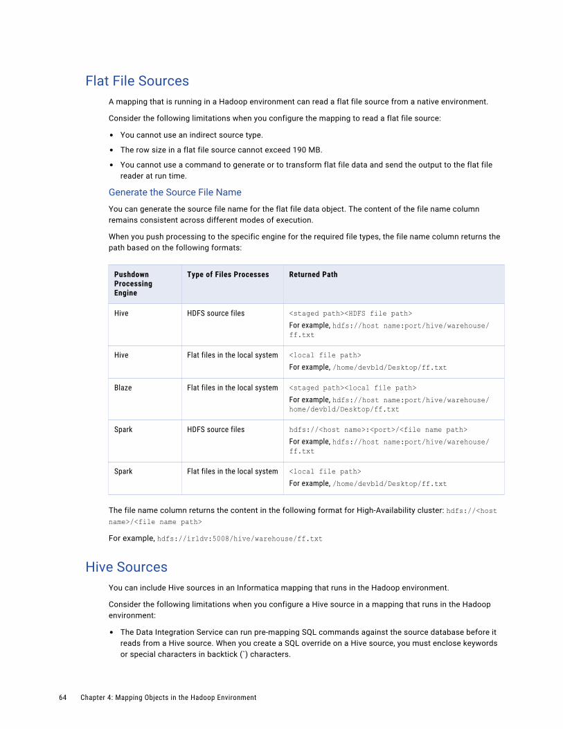
Flat File SourcesA mapping that is running in a Hadoop environment can read a flat file source from a native environment.
Consider the following limitations when you configure the mapping to read a flat file source:
• You cannot use an indirect source type.
• The row size in a flat file source cannot exceed 190 MB.
• You cannot use a command to generate or to transform flat file data and send the output to the flat file reader at run time.
Generate the Source File Name
You can generate the source file name for the flat file data object. The content of the file name column remains consistent across different modes of execution.
When you push processing to the specific engine for the required file types, the file name column returns the path based on the following formats:
Pushdown Processing Engine
Type of Files Processes Returned Path
Hive HDFS source files <staged path><HDFS file path>For example, hdfs://host name:port/hive/warehouse/ff.txt
Hive Flat files in the local system <local file path>For example, /home/devbld/Desktop/ff.txt
Blaze Flat files in the local system <staged path><local file path>For example, hdfs://host name:port/hive/warehouse/home/devbld/Desktop/ff.txt
Spark HDFS source files hdfs://<host name>:<port>/<file name path>For example, hdfs://host name:port/hive/warehouse/ff.txt
Spark Flat files in the local system <local file path>For example, /home/devbld/Desktop/ff.txt
The file name column returns the content in the following format for High-Availability cluster: hdfs://<host name>/<file name path>
For example, hdfs://irldv:5008/hive/warehouse/ff.txt
Hive SourcesYou can include Hive sources in an Informatica mapping that runs in the Hadoop environment.
Consider the following limitations when you configure a Hive source in a mapping that runs in the Hadoop environment:
• The Data Integration Service can run pre-mapping SQL commands against the source database before it reads from a Hive source. When you create a SQL override on a Hive source, you must enclose keywords or special characters in backtick (`) characters.
64 Chapter 4: Mapping Objects in the Hadoop Environment
• When you run a mapping with a Hive source in the Hadoop environment, references to a local path in pre-mapping SQL commands are relative to the Data Integration Service node. When you run a mapping with a Hive source in the native environment, references to local path in pre-mapping SQL commands are relative to the Hive server node.
• A mapping fails to validate when you configure post-mapping SQL commands. The Data Integration Service does not run post-mapping SQL commands against a Hive source.
• A mapping fails to run when you have Unicode characters in a Hive source definition.
• The third-party Hive JDBC driver does not return the correct precision and scale values for the Decimal data type. As a result, when you import Hive tables with a Decimal data type into the Developer tool, the Decimal data type precision is set to 38 and the scale is set to 0. Consider the following configuration rules and guidelines based on the version of Hive:
- Hive 0.11. Accept the default precision and scale for the Decimal data type in the Developer tool.
- Hive 0.12. Accept the default precision and scale for the Decimal data type in the Developer tool.
- Hive 0.12 with Cloudera CDH 5.0. You can configure the precision and scale fields for source columns with the Decimal data type in the Developer tool.
- Hive 0.13 and above. You can configure the precision and scale fields for source columns with the Decimal data type in the Developer tool.
- Hive 0.14 or above. The precision and scale used for the Decimal data type in the Hive database also appears in the Developer tool.
A mapping that runs on the Spark engine can have partitioned Hive source tables and bucketed sources.
Rules and Guidelines for Hive Sources on the Blaze EngineYou can include Hive sources in an Informatica mapping that runs on the Blaze engine.
Consider the following rules and guidelines when you configure a Hive source in a mapping that runs on the Blaze engine:
• Hive sources for a Blaze mapping include the TEXT, Sequence, Avro, RC, ORC, and Parquet storage formats.
• A mapping that runs on the Blaze engine can have bucketed Hive sources and Hive ACID tables.
• Hive ACID tables must be bucketed.
• The Blaze engine supports Hive tables that are enabled for locking.
• Hive sources can contain quoted identifiers in Hive table names, column names, and schema names.
• The TEXT storage format in a Hive source for a Blaze mapping can support ASCII characters as column delimiters and the newline characters as a row separator. You cannot use hex values of ASCII characters. For example, use a semicolon (;) instead of 3B.
• You can define an SQL override in the Hive source for a Blaze mapping.
• The Blaze engine can read from an RCFile as a Hive source. To read from an RCFile table, you must create the table with the SerDe clause.
• The Blaze engine can read from Hive tables that are compressed. To read from a compressed Hive table, you must set the TBLPROPERTIES clause.
RCFile as Hive Tables
The Blaze engine can read and write to RCFile as Hive tables. However, the Blaze engine supports only the ColumarSerDe SerDe. In Hortonworks, the default SerDe for an RCFile is LazyBinaryColumnarSerDe. To read and write to an RCFile table, you must create the table by specifying the SerDe as org.apache.hadoop.hive.serde2.columnar.ColumnarSerDe.
Sources in a Hadoop Environment 65
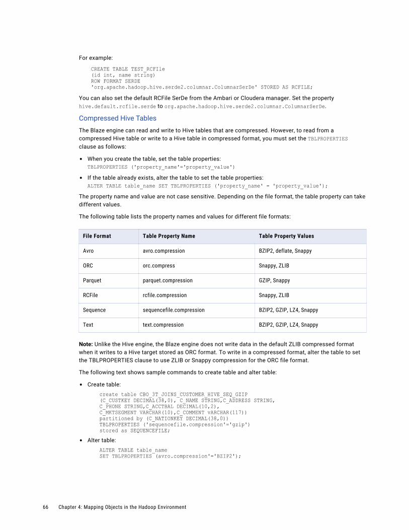
For example:
CREATE TABLE TEST_RCFIle (id int, name string)ROW FORMAT SERDE 'org.apache.hadoop.hive.serde2.columnar.ColumnarSerDe' STORED AS RCFILE;
You can also set the default RCFile SerDe from the Ambari or Cloudera manager. Set the property hive.default.rcfile.serde to org.apache.hadoop.hive.serde2.columnar.ColumnarSerDe.
Compressed Hive Tables
The Blaze engine can read and write to Hive tables that are compressed. However, to read from a compressed Hive table or write to a Hive table in compressed format, you must set the TBLPROPERTIES clause as follows:
• When you create the table, set the table properties:TBLPROPERTIES ('property_name'='property_value')
• If the table already exists, alter the table to set the table properties:ALTER TABLE table_name SET TBLPROPERTIES ('property_name' = 'property_value');
The property name and value are not case sensitive. Depending on the file format, the table property can take different values.
The following table lists the property names and values for different file formats:
File Format Table Property Name Table Property Values
Avro avro.compression BZIP2, deflate, Snappy
ORC orc.compress Snappy, ZLIB
Parquet parquet.compression GZIP, Snappy
RCFile rcfile.compression Snappy, ZLIB
Sequence sequencefile.compression BZIP2, GZIP, LZ4, Snappy
Text text.compression BZIP2, GZIP, LZ4, Snappy
Note: Unlike the Hive engine, the Blaze engine does not write data in the default ZLIB compressed format when it writes to a Hive target stored as ORC format. To write in a compressed format, alter the table to set the TBLPROPERTIES clause to use ZLIB or Snappy compression for the ORC file format.
The following text shows sample commands to create table and alter table:
• Create table:
create table CBO_3T_JOINS_CUSTOMER_HIVE_SEQ_GZIP(C_CUSTKEY DECIMAL(38,0), C_NAME STRING,C_ADDRESS STRING, C_PHONE STRING,C_ACCTBAL DECIMAL(10,2),C_MKTSEGMENT VARCHAR(10),C_COMMENT vARCHAR(117))partitioned by (C_NATIONKEY DECIMAL(38,0)) TBLPROPERTIES ('sequencefile.compression'='gzip') stored as SEQUENCEFILE;
• Alter table:
ALTER TABLE table_name SET TBLPROPERTIES (avro.compression'='BZIP2');
66 Chapter 4: Mapping Objects in the Hadoop Environment
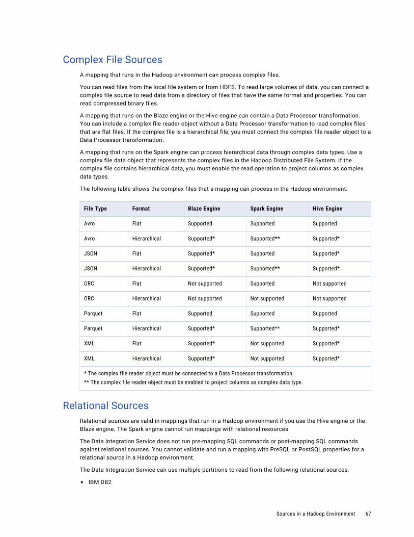
Complex File SourcesA mapping that runs in the Hadoop environment can process complex files.
You can read files from the local file system or from HDFS. To read large volumes of data, you can connect a complex file source to read data from a directory of files that have the same format and properties. You can read compressed binary files.
A mapping that runs on the Blaze engine or the Hive engine can contain a Data Processor transformation. You can include a complex file reader object without a Data Processor transformation to read complex files that are flat files. If the complex file is a hierarchical file, you must connect the complex file reader object to a Data Processor transformation.
A mapping that runs on the Spark engine can process hierarchical data through complex data types. Use a complex file data object that represents the complex files in the Hadoop Distributed File System. If the complex file contains hierarchical data, you must enable the read operation to project columns as complex data types.
The following table shows the complex files that a mapping can process in the Hadoop environment:
File Type Format Blaze Engine Spark Engine Hive Engine
Avro Flat Supported Supported Supported
Avro Hierarchical Supported* Supported** Supported*
JSON Flat Supported* Supported Supported*
JSON Hierarchical Supported* Supported** Supported*
ORC Flat Not supported Supported Not supported
ORC Hierarchical Not supported Not supported Not supported
Parquet Flat Supported Supported Supported
Parquet Hierarchical Supported* Supported** Supported*
XML Flat Supported* Not supported Supported*
XML Hierarchical Supported* Not supported Supported*
* The complex file reader object must be connected to a Data Processor transformation.** The complex file reader object must be enabled to project columns as complex data type.
Relational SourcesRelational sources are valid in mappings that run in a Hadoop environment if you use the Hive engine or the Blaze engine. The Spark engine cannot run mappings with relational resources.
The Data Integration Service does not run pre-mapping SQL commands or post-mapping SQL commands against relational sources. You cannot validate and run a mapping with PreSQL or PostSQL properties for a relational source in a Hadoop environment.
The Data Integration Service can use multiple partitions to read from the following relational sources:
• IBM DB2
Sources in a Hadoop Environment 67
• Oracle
Note: You do not have to set maximum parallelism for the Data Integration Service to use multiple partitions in the Hadoop environment.
Sqoop SourcesSqoop sources are valid in mappings in a Hadoop environment.
You can include a JDBC-compliant database as a Sqoop source in an Informatica mapping that runs in a Hadoop environment:
For example, you can include the following sources in a Sqoop mapping:
• Aurora
• Greenplum
• IBM DB2
• IBM DB2 for z/OS
• Microsoft SQL Server
• Netezza
• Oracle
• Teradata
Rules and Guidelines for Sqoop SourcesConsider the following rules and guidelines when you configure a Sqoop source in a mapping:
• To override the default query in a mapping with an advanced query, you must define a mapping parameter and set its value to $CONDITIONS. You must then include $CONDITIONS in the WHERE clause of the custom query.
• If you define a custom query, you must verify that the metadata of the custom query matches the metadata of the source object. Otherwise, Sqoop might write blank values to the target.
• If you specify a sort condition in a mapping, the Data Integration Service ignores the Order By condition.
• You cannot sort columns in a Sqoop source.
• You cannot read distinct rows from a Sqoop source.
• When you enable OraOop and configure an advanced query to read data from an Oracle source through Sqoop, the mapping fails on the Spark engine.
• When you read data from an Oracle source through Sqoop and run the mapping on the Blaze or Spark engine, Sqoop treats the owner name as case sensitive.
• Sqoop uses the values that you configure in the User Name and Password fields of the JDBC connection. If you configure the --username or --password argument in a JDBC connection or mapping, Sqoop ignores the arguments. If you create a password file to access a database, Sqoop ignores the password file.
68 Chapter 4: Mapping Objects in the Hadoop Environment
Targets in a Hadoop EnvironmentYou can push a mapping to the Hadoop environment that includes a target from the native environment or from the Hadoop environment. Some sources have limitations when you reference them in the Hadoop environment.
You can run mappings with the following targets in a Hadoop environment:
• Complex files
• Flat file (native)
• Greenplum
• HBase
• HDFS flat file
• Hive
• IBM DB2
• Netezza
• ODBC
• Oracle
• Sqoop targets
• Teradata
A mapping that runs with the Spark engine can have partitioned Hive target tables and bucketed targets.
When a mapping runs in the Hadoop environment, an HDFS target or a Hive target cannot reside on a remote cluster. A remote cluster is a cluster that is remote from the machine that the Hadoop connection references in the mapping.
Flat File TargetsA mapping that is running in a Hadoop environment can write to a flat file target that is in a native environment.
Consider the following limitations when you configure a flat file target in a mapping that runs in a Hadoop environment:
• The Data Integration Service truncates the target files and reject files before writing the data. When you use a flat file target, you cannot append output data to target files and reject files.
• The Data Integration Service can write to a file output for a flat file target. When you have a flat file target in a mapping, you cannot write data to a command.
HDFS Flat File TargetsHDFS flat file targets are valid in mappings that run in a Hadoop environment.
When you use a HDFS flat file target in a mapping, you must specify the full path that includes the output file directory and file name. The Data Integration Service might generate multiple output files in the output directory when you run the mapping in a Hadoop environment.
Targets in a Hadoop Environment 69
Hive TargetsA mapping that is running in the Hadoop environment can write to a Hive target.
The Spark engine can write to bucketed Hive targets. Bucketing and partitioning of Hive tables can improve performance by reducing data shuffling and sorting.
Consider the following restrictions when you configure a Hive target in a mapping that runs in the Hadoop environment:
• The Data Integration Service does not run pre-mapping or post-mapping SQL commands against a Hive target. You cannot validate and run a mapping with PreSQL or PostSQL properties for a Hive target.
• A mapping fails to run if the Hive target definition differs in the number and order of the columns from the relational table in the Hive database.
• A mapping fails to run when you use Unicode characters in a Hive target definition.
• You must truncate the target table to overwrite data to a Hive table with Hive version 0.7. The Data Integration Service ignores write, update override, delete, insert, and update strategy properties when it writes data to a Hive target.
• When you set up a dynamic target for a partitioned Hive table, the value used for the partition is the final column in the table. If the table has a dynamic partition column, the final column of the table is the dynamic partition column. To use a different column for the partition, move it to the last column of the table. If the table has multiple partition columns, the dynamic partition values are selected from the last columns of the upstream transformation.
• The Data Integration Service can truncate the partition in the Hive target in which the data is being inserted. You must choose to both truncate the partition in the Hive target and truncate the target table.
In a mapping that runs on the Spark engine or the Blaze engine, you can create a custom DDL query that creates or replaces a Hive table at run time. However, with the Blaze engine, you cannot use a backtick (`) character in the DDL query. The backtick character is required in HiveQL when you include special characters or keywords in a query.
When a mapping creates or replaces a Hive table, the type of table that the mapping creates depends on the run-time engine that you use to run the mapping.
The following table shows the table type for each run-time engine:
Run-Time Engine Resulting Table Type
Blaze MANAGED_TABLE
Spark EXTERNAL_TABLE
Hive MANAGED_TABLE
Rules and Guidelines for Hive Targets on the Blaze EngineYou can include Hive targets in an Informatica mapping that runs on the Blaze engine.
Consider the following rules and guidelines when you configure a Hive target in a mapping that runs on the Blaze engine:
• A mapping that runs on the Blaze engine can have partitioned and bucketed Hive tables as targets. However, if you append data to a bucketed table, the Blaze engine overwrites the data in the bucketed target.
• Mappings that run on the Blaze engine can read and write to sorted targets.
70 Chapter 4: Mapping Objects in the Hadoop Environment
• The Blaze engine supports Hive tables that are enabled for locking.
• The Blaze engine can create or replace Hive target tables and truncate the partition in the Hive target table. You must choose to both truncate the partition in the Hive target and truncate the target table.
• A mapping that runs on the Blaze engine can write to Hive ACID tables. To write to a Hive ACID table, the mapping must contain an Update Strategy transformation connected to the Hive target. The update strategy expression must flag each row for insert.
• The Blaze engine can write to an RCFile as a Hive target. To write to an RCFile table, you must create the table with the SerDe clause.
• The Blaze engine can write to Hive tables that are compressed. To write to a Hive table in compressed format, you must set the TBLPROPERTIES clause.
RCFile as Hive Tables
The Blaze engine can read and write to RCFile as Hive tables. However, the Blaze engine supports only the ColumarSerDe SerDe. In Hortonworks, the default SerDe for an RCFile is LazyBinaryColumnarSerDe. To read and write to an RCFile table, you must create the table by specifying the SerDe as org.apache.hadoop.hive.serde2.columnar.ColumnarSerDe.
For example:
CREATE TABLE TEST_RCFIle (id int, name string)ROW FORMAT SERDE 'org.apache.hadoop.hive.serde2.columnar.ColumnarSerDe' STORED AS RCFILE;
You can also set the default RCFile SerDe from the Ambari or Cloudera manager. Set the property hive.default.rcfile.serde to org.apache.hadoop.hive.serde2.columnar.ColumnarSerDe.
Compressed Hive Tables
The Blaze engine can read and write to Hive tables that are compressed. However, to read from a compressed Hive table or write to a Hive table in compressed format, you must set the TBLPROPERTIES clause as follows:
• When you create the table, set the table properties:TBLPROPERTIES ('property_name'='property_value')
• If the table already exists, alter the table to set the table properties:ALTER TABLE table_name SET TBLPROPERTIES ('property_name' = 'property_value');
The property name and value are not case sensitive. Depending on the file format, the table property can take different values.
The following table lists the property names and values for different file formats:
File Format Table Property Name Table Property Values
Avro avro.compression BZIP2, deflate, Snappy
ORC orc.compress Snappy, ZLIB
Parquet parquet.compression GZIP, Snappy
RCFile rcfile.compression Snappy, ZLIB
Sequence sequencefile.compression BZIP2, GZIP, LZ4, Snappy
Text text.compression BZIP2, GZIP, LZ4, Snappy
Targets in a Hadoop Environment 71
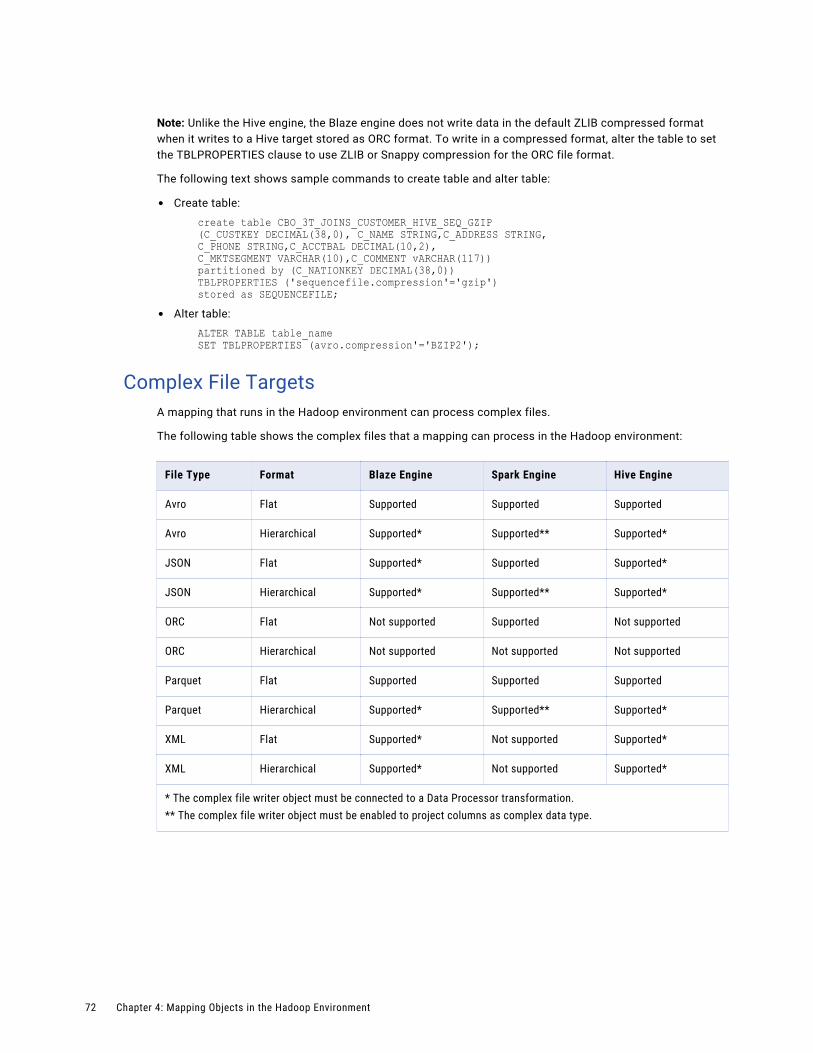
Note: Unlike the Hive engine, the Blaze engine does not write data in the default ZLIB compressed format when it writes to a Hive target stored as ORC format. To write in a compressed format, alter the table to set the TBLPROPERTIES clause to use ZLIB or Snappy compression for the ORC file format.
The following text shows sample commands to create table and alter table:
• Create table:
create table CBO_3T_JOINS_CUSTOMER_HIVE_SEQ_GZIP(C_CUSTKEY DECIMAL(38,0), C_NAME STRING,C_ADDRESS STRING, C_PHONE STRING,C_ACCTBAL DECIMAL(10,2),C_MKTSEGMENT VARCHAR(10),C_COMMENT vARCHAR(117))partitioned by (C_NATIONKEY DECIMAL(38,0)) TBLPROPERTIES ('sequencefile.compression'='gzip') stored as SEQUENCEFILE;
• Alter table:
ALTER TABLE table_name SET TBLPROPERTIES (avro.compression'='BZIP2');
Complex File TargetsA mapping that runs in the Hadoop environment can process complex files.
The following table shows the complex files that a mapping can process in the Hadoop environment:
File Type Format Blaze Engine Spark Engine Hive Engine
Avro Flat Supported Supported Supported
Avro Hierarchical Supported* Supported** Supported*
JSON Flat Supported* Supported Supported*
JSON Hierarchical Supported* Supported** Supported*
ORC Flat Not supported Supported Not supported
ORC Hierarchical Not supported Not supported Not supported
Parquet Flat Supported Supported Supported
Parquet Hierarchical Supported* Supported** Supported*
XML Flat Supported* Not supported Supported*
XML Hierarchical Supported* Not supported Supported*
* The complex file writer object must be connected to a Data Processor transformation.** The complex file writer object must be enabled to project columns as complex data type.
72 Chapter 4: Mapping Objects in the Hadoop Environment

Relational TargetsRelational targets are valid in mappings in a Hadoop environment if you use the Hive or Blaze engine. The Spark engine cannot run mappings with relational targets.
The Data Integration Service does not run pre-mapping SQL commands or post-mapping SQL commands against relational targets in a Hadoop environment. You cannot validate and run a mapping with PreSQL or PostSQL properties for a relational target in a Hadoop environment.
The Data Integration Service can use multiple partitions to write to the following relational targets:
• IBM DB2
• Oracle
Note: You do not have to set maximum parallelism for the Data Integration Service to use multiple partitions in the Hadoop environment.
Sqoop TargetsSqoop targets are valid in mappings in a Hadoop environment.
You can include a JDBC-compliant database as a Sqoop target in an Informatica mapping that runs in a Hadoop environment:
For example, you can include the following targets in a Sqoop mapping:
• Aurora
• Greenplum
• IBM DB2
• IBM DB2 for z/OS
• Microsoft SQL Server
• Netezza
• Oracle
• Teradata
You can insert data. You cannot update or delete data in a target. If you configure update arguments, Sqoop ignores them.
Rules and Guidelines for Sqoop TargetsConsider the following rules and guidelines when you configure a Sqoop target in a mapping:
• If a column name or table name contains a special character, the Sqoop export process fails.
• If you configure the Maintain Row Order property for a Sqoop target, the Data Integration Service ignores the property.
• When you run a Sqoop mapping on the Blaze engine, verify that you have not deleted any target port from the mapping. Otherwise, the mapping fails.
• When you export null data to a Microsoft SQL Server column that is defined as not null, the Data Integration Service fails the Sqoop mapping on the Blaze engine instead of rejecting and writing the null data to the bad file.
• When you write data to an Oracle target through Sqoop and run the mapping on the Blaze or Spark engine, Sqoop treats the owner name as case sensitive.
Targets in a Hadoop Environment 73
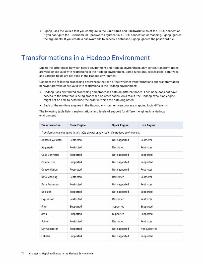
• Sqoop uses the values that you configure in the User Name and Password fields of the JDBC connection. If you configure the --username or --password argument in a JDBC connection or mapping, Sqoop ignores the arguments. If you create a password file to access a database, Sqoop ignores the password file.
Transformations in a Hadoop EnvironmentDue to the differences between native environment and Hadoop environment, only certain transformations are valid or are valid with restrictions in the Hadoop environment. Some functions, expressions, data types, and variable fields are not valid in the Hadoop environment.
Consider the following processing differences that can affect whether transformations and transformation behavior are valid or are valid with restrictions in the Hadoop environment:
• Hadoop uses distributed processing and processes data on different nodes. Each node does not have access to the data that is being processed on other nodes. As a result, the Hadoop execution engine might not be able to determine the order in which the data originated.
• Each of the run-time engines in the Hadoop environment can process mapping logic differently.
The following table lists transformations and levels of support for different engines in a Hadoop environment:
Transformation Blaze Engine Spark Engine Hive Engine
Transformations not listed in this table are not supported in the Hadoop environment.
Address Validator Restricted Not supported Restricted
Aggregator Restricted Restricted Restricted
Case Converter Supported Not supported Supported
Comparison Supported Not supported Supported
Consolidation Restricted Not supported Restricted
Data Masking Restricted Restricted Restricted
Data Processor Restricted Not supported Restricted
Decision Supported Not supported Supported
Expression Restricted Restricted Restricted
Filter Supported Supported Supported
Java Supported Supported Supported
Joiner Restricted Restricted Restricted
Key Generator Supported Not supported Not supported
Labeler Supported Not supported Supported
74 Chapter 4: Mapping Objects in the Hadoop Environment
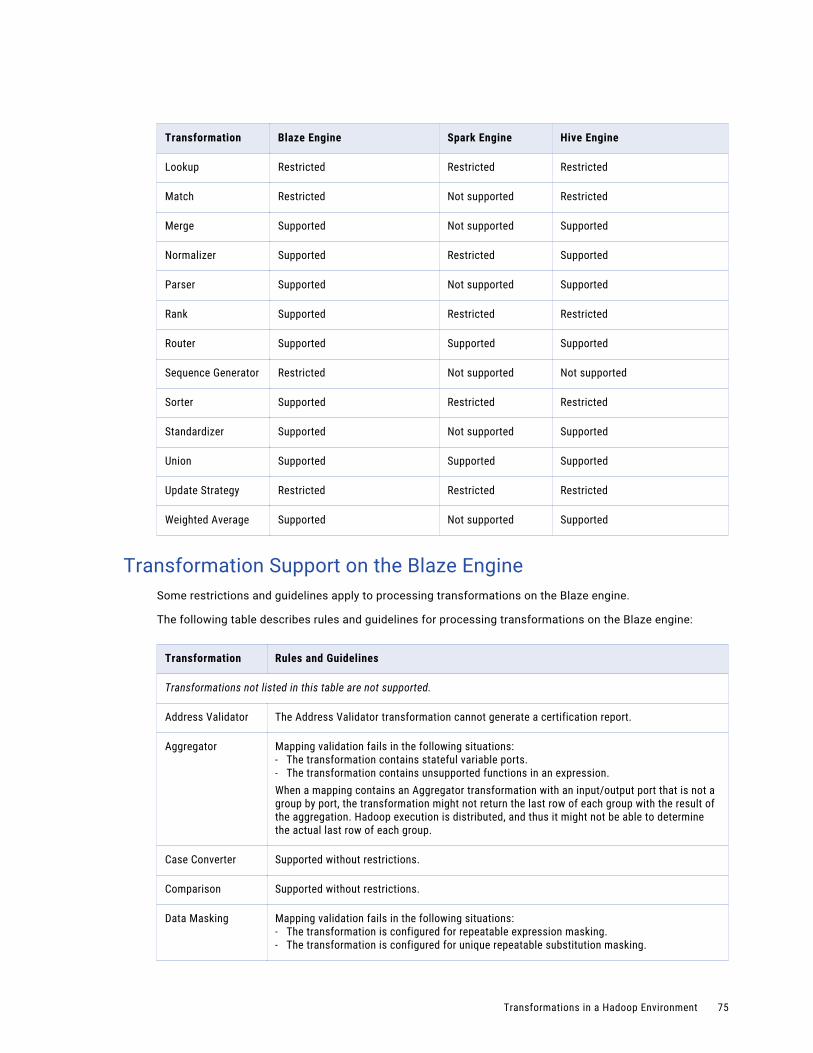
Transformation Blaze Engine Spark Engine Hive Engine
Lookup Restricted Restricted Restricted
Match Restricted Not supported Restricted
Merge Supported Not supported Supported
Normalizer Supported Restricted Supported
Parser Supported Not supported Supported
Rank Supported Restricted Restricted
Router Supported Supported Supported
Sequence Generator Restricted Not supported Not supported
Sorter Supported Restricted Restricted
Standardizer Supported Not supported Supported
Union Supported Supported Supported
Update Strategy Restricted Restricted Restricted
Weighted Average Supported Not supported Supported
Transformation Support on the Blaze EngineSome restrictions and guidelines apply to processing transformations on the Blaze engine.
The following table describes rules and guidelines for processing transformations on the Blaze engine:
Transformation Rules and Guidelines
Transformations not listed in this table are not supported.
Address Validator The Address Validator transformation cannot generate a certification report.
Aggregator Mapping validation fails in the following situations:- The transformation contains stateful variable ports.- The transformation contains unsupported functions in an expression.When a mapping contains an Aggregator transformation with an input/output port that is not a group by port, the transformation might not return the last row of each group with the result of the aggregation. Hadoop execution is distributed, and thus it might not be able to determine the actual last row of each group.
Case Converter Supported without restrictions.
Comparison Supported without restrictions.
Data Masking Mapping validation fails in the following situations:- The transformation is configured for repeatable expression masking.- The transformation is configured for unique repeatable substitution masking.
Transformations in a Hadoop Environment 75
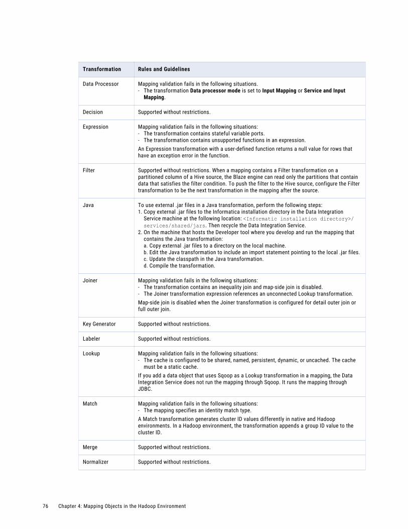
Transformation Rules and Guidelines
Data Processor Mapping validation fails in the following situations.- The transformation Data processor mode is set to Input Mapping or Service and Input
Mapping.
Decision Supported without restrictions.
Expression Mapping validation fails in the following situations:- The transformation contains stateful variable ports.- The transformation contains unsupported functions in an expression.An Expression transformation with a user-defined function returns a null value for rows that have an exception error in the function.
Filter Supported without restrictions. When a mapping contains a Filter transformation on a partitioned column of a Hive source, the Blaze engine can read only the partitions that contain data that satisfies the filter condition. To push the filter to the Hive source, configure the Filter transformation to be the next transformation in the mapping after the source.
Java To use external .jar files in a Java transformation, perform the following steps:1. Copy external .jar files to the Informatica installation directory in the Data Integration
Service machine at the following location: <Informatic installation directory>/services/shared/jars. Then recycle the Data Integration Service.
2. On the machine that hosts the Developer tool where you develop and run the mapping that contains the Java transformation:a. Copy external .jar files to a directory on the local machine.b. Edit the Java transformation to include an import statement pointing to the local .jar files.c. Update the classpath in the Java transformation.d. Compile the transformation.
Joiner Mapping validation fails in the following situations:- The transformation contains an inequality join and map-side join is disabled.- The Joiner transformation expression references an unconnected Lookup transformation.Map-side join is disabled when the Joiner transformation is configured for detail outer join or full outer join.
Key Generator Supported without restrictions.
Labeler Supported without restrictions.
Lookup Mapping validation fails in the following situations:- The cache is configured to be shared, named, persistent, dynamic, or uncached. The cache
must be a static cache.If you add a data object that uses Sqoop as a Lookup transformation in a mapping, the Data Integration Service does not run the mapping through Sqoop. It runs the mapping through JDBC.
Match Mapping validation fails in the following situations:- The mapping specifies an identity match type.A Match transformation generates cluster ID values differently in native and Hadoop environments. In a Hadoop environment, the transformation appends a group ID value to the cluster ID.
Merge Supported without restrictions.
Normalizer Supported without restrictions.
76 Chapter 4: Mapping Objects in the Hadoop Environment
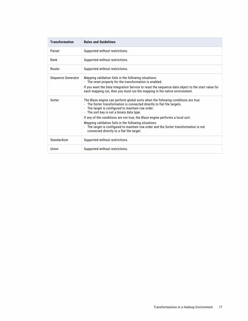
Transformation Rules and Guidelines
Parser Supported without restrictions.
Rank Supported without restrictions.
Router Supported without restrictions.
Sequence Generator Mapping validation fails in the following situations:- The reset property for the transformation is enabled.If you want the Data Integration Service to reset the sequence data object to the start value for each mapping run, then you must run the mapping in the native environment.
Sorter The Blaze engine can perform global sorts when the following conditions are true:- The Sorter transformation is connected directly to flat file targets.- The target is configured to maintain row order.- The sort key is not a binary data type.If any of the conditions are not true, the Blaze engine performs a local sort.Mapping validation fails in the following situations:- The target is configured to maintain row order and the Sorter transformation is not
connected directly to a flat file target.
Standardizer Supported without restrictions.
Union Supported without restrictions.
Transformations in a Hadoop Environment 77
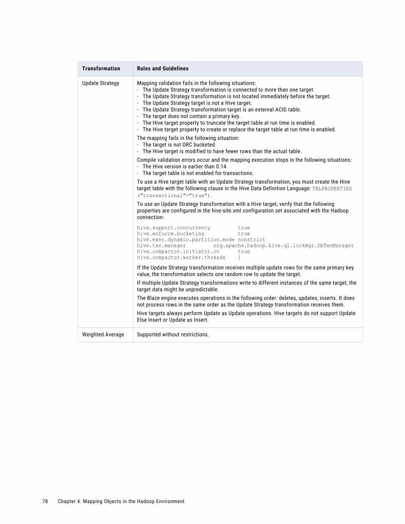
Transformation Rules and Guidelines
Update Strategy Mapping validation fails in the following situations:- The Update Strategy transformation is connected to more than one target.- The Update Strategy transformation is not located immediately before the target.- The Update Strategy target is not a Hive target.- The Update Strategy transformation target is an external ACID table.- The target does not contain a primary key.- The Hive target property to truncate the target table at run time is enabled.- The Hive target property to create or replace the target table at run time is enabled.The mapping fails in the following situation:- The target is not ORC bucketed.- The Hive target is modified to have fewer rows than the actual table.Compile validation errors occur and the mapping execution stops in the following situations:- The Hive version is earlier than 0.14.- The target table is not enabled for transactions.To use a Hive target table with an Update Strategy transformation, you must create the Hive target table with the following clause in the Hive Data Definition Language: TBLPROPERTIES ("transactional"="true").To use an Update Strategy transformation with a Hive target, verify that the following properties are configured in the hive-site.xml configuration set associated with the Hadoop connection:
hive.support.concurrency truehive.enforce.bucketing truehive.exec.dynamic.partition.mode nonstricthive.txn.manager org.apache.hadoop.hive.ql.lockmgr.DbTxnManagerhive.compactor.initiator.on truehive.compactor.worker.threads 1 If the Update Strategy transformation receives multiple update rows for the same primary key value, the transformation selects one random row to update the target.If multiple Update Strategy transformations write to different instances of the same target, the target data might be unpredictable.The Blaze engine executes operations in the following order: deletes, updates, inserts. It does not process rows in the same order as the Update Strategy transformation receives them.Hive targets always perform Update as Update operations. Hive targets do not support Update Else Insert or Update as Insert.
Weighted Average Supported without restrictions.
78 Chapter 4: Mapping Objects in the Hadoop Environment

Transformation Support on the Spark EngineSome restrictions and guidelines apply to processing transformations on the Spark engine.
The following table describes rules and guidelines for the transformations that are supported on the Spark engine:
Transformation Rules and Guidelines
Transformations not listed in this table are not supported.
Aggregator Mapping validation fails in the following situations:- The transformation contains stateful variable ports.- The transformation contains unsupported functions in an expression.When a mapping contains an Aggregator transformation with an input/output port that is not a group by port, the transformation might not return the last row of each group with the result of the aggregation. Hadoop execution is distributed, and thus it might not be able to determine the actual last row of each group.
Data Masking Mapping validation fails in the following situations:- The transformation is configured for repeatable expression masking.- The transformation is configured for unique repeatable substitution masking.
Expression Mapping validation fails in the following situations:- The transformation contains stateful variable ports.- The transformation contains unsupported functions in an expression.If an expression results in numerical errors, such as division by zero or SQRT of a negative number, it returns an infinite or an NaN value. In the native environment, the expression returns null values and the rows do not appear in the output.
Filter Supported without restrictions.
Transformations in a Hadoop Environment 79
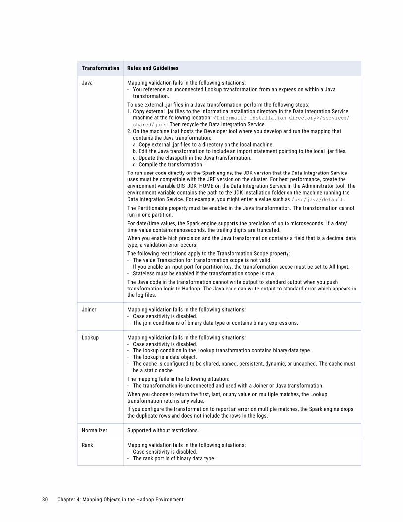
Transformation Rules and Guidelines
Java Mapping validation fails in the following situations:- You reference an unconnected Lookup transformation from an expression within a Java
transformation.To use external .jar files in a Java transformation, perform the following steps:1. Copy external .jar files to the Informatica installation directory in the Data Integration Service
machine at the following location: <Informatic installation directory>/services/shared/jars. Then recycle the Data Integration Service.
2. On the machine that hosts the Developer tool where you develop and run the mapping that contains the Java transformation:a. Copy external .jar files to a directory on the local machine.b. Edit the Java transformation to include an import statement pointing to the local .jar files.c. Update the classpath in the Java transformation.d. Compile the transformation.
To run user code directly on the Spark engine, the JDK version that the Data Integration Service uses must be compatible with the JRE version on the cluster. For best performance, create the environment variable DIS_JDK_HOME on the Data Integration Service in the Administrator tool. The environment variable contains the path to the JDK installation folder on the machine running the Data Integration Service. For example, you might enter a value such as /usr/java/default.The Partitionable property must be enabled in the Java transformation. The transformation cannot run in one partition.For date/time values, the Spark engine supports the precision of up to microseconds. If a date/time value contains nanoseconds, the trailing digits are truncated.When you enable high precision and the Java transformation contains a field that is a decimal data type, a validation error occurs.The following restrictions apply to the Transformation Scope property:- The value Transaction for transformation scope is not valid.- If you enable an input port for partition key, the transformation scope must be set to All Input.- Stateless must be enabled if the transformation scope is row.The Java code in the transformation cannot write output to standard output when you push transformation logic to Hadoop. The Java code can write output to standard error which appears in the log files.
Joiner Mapping validation fails in the following situations:- Case sensitivity is disabled.- The join condition is of binary data type or contains binary expressions.
Lookup Mapping validation fails in the following situations:- Case sensitivity is disabled.- The lookup condition in the Lookup transformation contains binary data type.- The lookup is a data object.- The cache is configured to be shared, named, persistent, dynamic, or uncached. The cache must
be a static cache.The mapping fails in the following situation:- The transformation is unconnected and used with a Joiner or Java transformation.When you choose to return the first, last, or any value on multiple matches, the Lookup transformation returns any value.If you configure the transformation to report an error on multiple matches, the Spark engine drops the duplicate rows and does not include the rows in the logs.
Normalizer Supported without restrictions.
Rank Mapping validation fails in the following situations:- Case sensitivity is disabled.- The rank port is of binary data type.
80 Chapter 4: Mapping Objects in the Hadoop Environment

Transformation Rules and Guidelines
Router Supported without restrictions.
Sorter Mapping validation fails in the following situations:- Case sensitivity is disabled.The Data Integration Service logs a warning and ignores the Sorter transformation in the following situations:- There is a type mismatch in between the target and the Sorter transformation sort keys.- The transformation contains sort keys that are not connected to the target.- The Write transformation is not configured to maintain row order.- The transformation is not directly upstream from the Write transformation.The Data Integration Service treats null values as high even if you configure the transformation to treat null values as low.
Union Supported without restrictions.
Update Strategy Mapping validation fails in the following situations:- The Update Strategy transformation is connected to more than one target.- The Update Strategy transformation is not located immediately before the target.- The Update Strategy target is not a Hive target.- The Update Strategy transformation target is an external ACID table.- The target does not contain a connected primary key.- The Hive target property to truncate the target table at run time is enabled.- The Hive target property to create or replace the target table at run time is enabled.The mapping fails in the following situations:- The target table is not enabled for transactions.- The target is not ORC bucketed.The Update Strategy transformation does not forward rejected rows to the next transformation.To use a Hive target table with an Update Strategy transformation, you must create the Hive target table with the following clause in the Hive Data Definition Language: TBLPROPERTIES ("transactional"="true").To use an Update Strategy transformation with a Hive target, verify that the following properties are configured in the hive-site.xml configuration set associated with the Hadoop connection:
hive.support.concurrency truehive.enforce.bucketing truehive.exec.dynamic.partition.mode nonstricthive.txn.manager org.apache.hadoop.hive.ql.lockmgr.DbTxnManagerhive.compactor.initiator.on truehive.compactor.worker.threads 1 If the Update Strategy transformation receives multiple update rows for the same primary key value, the transformation selects one random row to update the target.If multiple Update Strategy transformations write to different instances of the same target, the target data might be unpredictable.The Spark engine executes operations in the following order: deletes, updates, inserts. It does not process rows in the same order as the Update Strategy transformation receives them.Hive targets always perform Update as Update operations. Hive targets do not support Update Else Insert or Update as Insert.
Transformation Support on the Hive EngineSome restrictions and guidelines apply to processing transformations on the Hive engine.
Transformations in a Hadoop Environment 81
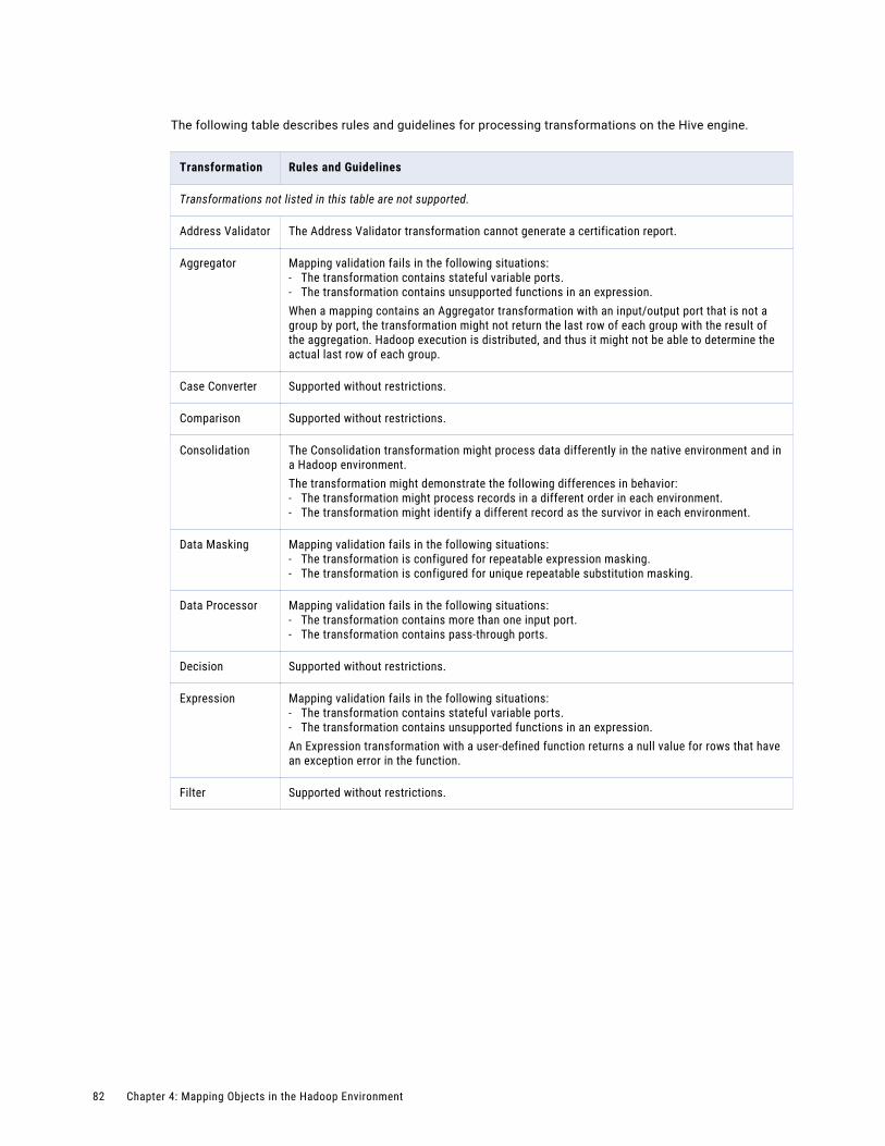
The following table describes rules and guidelines for processing transformations on the Hive engine.
Transformation Rules and Guidelines
Transformations not listed in this table are not supported.
Address Validator The Address Validator transformation cannot generate a certification report.
Aggregator Mapping validation fails in the following situations:- The transformation contains stateful variable ports.- The transformation contains unsupported functions in an expression.When a mapping contains an Aggregator transformation with an input/output port that is not a group by port, the transformation might not return the last row of each group with the result of the aggregation. Hadoop execution is distributed, and thus it might not be able to determine the actual last row of each group.
Case Converter Supported without restrictions.
Comparison Supported without restrictions.
Consolidation The Consolidation transformation might process data differently in the native environment and in a Hadoop environment.The transformation might demonstrate the following differences in behavior:- The transformation might process records in a different order in each environment.- The transformation might identify a different record as the survivor in each environment.
Data Masking Mapping validation fails in the following situations:- The transformation is configured for repeatable expression masking.- The transformation is configured for unique repeatable substitution masking.
Data Processor Mapping validation fails in the following situations:- The transformation contains more than one input port.- The transformation contains pass-through ports.
Decision Supported without restrictions.
Expression Mapping validation fails in the following situations:- The transformation contains stateful variable ports.- The transformation contains unsupported functions in an expression.An Expression transformation with a user-defined function returns a null value for rows that have an exception error in the function.
Filter Supported without restrictions.
82 Chapter 4: Mapping Objects in the Hadoop Environment
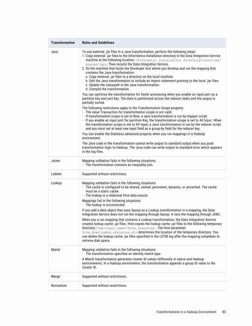
Transformation Rules and Guidelines
Java To use external .jar files in a Java transformation, perform the following steps:1. Copy external .jar files to the Informatica installation directory in the Data Integration Service
machine at the following location: <Informatic installation directory>/services/shared/jars. Then recycle the Data Integration Service.
2. On the machine that hosts the Developer tool where you develop and run the mapping that contains the Java transformation:a. Copy external .jar files to a directory on the local machine.b. Edit the Java transformation to include an import statement pointing to the local .jar files.c. Update the classpath in the Java transformation.d. Compile the transformation.
You can optimize the transformation for faster processing when you enable an input port as a partition key and sort key. The data is partitioned across the reducer tasks and the output is partially sorted.The following restrictions apply to the Transformation Scope property:- The value Transaction for transformation scope is not valid.- If transformation scope is set to Row, a Java transformation is run by mapper script.- If you enable an input port for partition Key, the transformation scope is set to All Input. When
the transformation scope is set to All Input, a Java transformation is run by the reducer script and you must set at least one input field as a group-by field for the reducer key.
You can enable the Stateless advanced property when you run mappings in a Hadoop environment.The Java code in the transformation cannot write output to standard output when you push transformation logic to Hadoop. The Java code can write output to standard error which appears in the log files.
Joiner Mapping validation fails in the following situations:- The transformation contains an inequality join.
Labeler Supported without restrictions.
Lookup Mapping validation fails in the following situations:- The cache is configured to be shared, named, persistent, dynamic, or uncached. The cache
must be a static cache.- The lookup is a relational Hive data source.Mappings fail in the following situations:- The lookup is unconnected.If you add a data object that uses Sqoop as a Lookup transformation in a mapping, the Data Integration Service does not run the mapping through Sqoop. It runs the mapping through JDBC.When you a run mapping that contains a Lookup transformation, the Data Integration Service creates lookup cache .jar files. Hive copies the lookup cache .jar files to the following temporary directory:/tmp/<user_name>/hive_resources . The Hive parameter hive.downloaded.resources.dir determines the location of the temporary directory. You can delete the lookup cache .jar files specified in the LDTM log after the mapping completes to retrieve disk space.
Match Mapping validation fails in the following situations:- The transformation specifies an identity match type.A Match transformation generates cluster ID values differently in native and Hadoop environments. In a Hadoop environment, the transformation appends a group ID value to the cluster ID.
Merge Supported without restrictions.
Normalizer Supported without restrictions.
Transformations in a Hadoop Environment 83
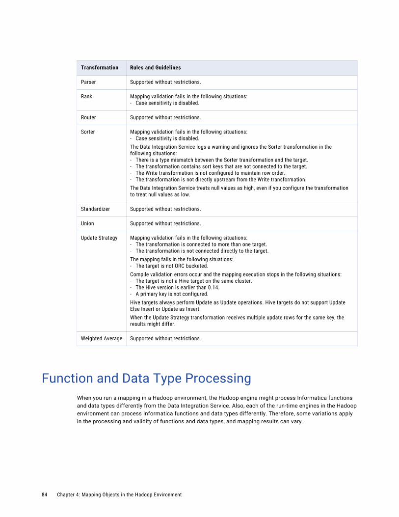
Transformation Rules and Guidelines
Parser Supported without restrictions.
Rank Mapping validation fails in the following situations:- Case sensitivity is disabled.
Router Supported without restrictions.
Sorter Mapping validation fails in the following situations:- Case sensitivity is disabled.The Data Integration Service logs a warning and ignores the Sorter transformation in the following situations:- There is a type mismatch between the Sorter transformation and the target.- The transformation contains sort keys that are not connected to the target.- The Write transformation is not configured to maintain row order.- The transformation is not directly upstream from the Write transformation.The Data Integration Service treats null values as high, even if you configure the transformation to treat null values as low.
Standardizer Supported without restrictions.
Union Supported without restrictions.
Update Strategy Mapping validation fails in the following situations:- The transformation is connected to more than one target.- The transformation is not connected directly to the target.The mapping fails in the following situations:- The target is not ORC bucketed.Compile validation errors occur and the mapping execution stops in the following situations:- The target is not a Hive target on the same cluster.- The Hive version is earlier than 0.14.- A primary key is not configured.Hive targets always perform Update as Update operations. Hive targets do not support Update Else Insert or Update as Insert.When the Update Strategy transformation receives multiple update rows for the same key, the results might differ.
Weighted Average Supported without restrictions.
Function and Data Type ProcessingWhen you run a mapping in a Hadoop environment, the Hadoop engine might process Informatica functions and data types differently from the Data Integration Service. Also, each of the run-time engines in the Hadoop environment can process Informatica functions and data types differently. Therefore, some variations apply in the processing and validity of functions and data types, and mapping results can vary.
84 Chapter 4: Mapping Objects in the Hadoop Environment

Rules and Guidelines for Spark Engine ProcessingSome restrictions and guidelines apply to processing Informatica functions on the Spark engine.
Important: When you push a mapping to the Hadoop environment, the engine that processes the mapping uses a set of rules different from the Data Integration Service. As a result, the mapping results can vary based on the rules that the engine uses. This topic contains some processing differences that Informatica discovered through internal testing and usage. Informatica does not test all the rules of the third-party engines and cannot provide an extensive list of the differences.
Consider the following rules and guidelines for function and data type processing on the Spark engine:
• The Spark engine and the Data Integration Service process overflow values differently. The Spark engine processing rules might differ from the rules that the Data Integration Service uses. As a result, mapping results can vary between the native and Hadoop environment when the Spark engine processes an overflow. Consider the following processing variation for Spark:
- If an expression results in numerical errors, such as division by zero or SQRT of a negative number, it returns an infinite or an NaN value. In the native environment, the expression returns null values and the rows do not appear in the output.
• The Spark engine and the Data Integration Service process data type conversions differently. As a result, mapping results can vary between the native and Hadoop environment when the Spark engine performs a data type conversion. Consider the following processing variations for Spark:
- The results of arithmetic operations on floating point types, such as Decimal, can vary up to 0.1 percent between the native environment and a Hadoop environment.
- The Spark engine ignores the scale argument of the TO_DECIMAL function. The function returns a value with the same scale as the input value.
- When the scale of a double or decimal value is smaller than the configured scale, the Spark engine trims the trailing zeros.
- The Spark engine cannot process dates to the nanosecond. It can return a precision for date/time data up to the microsecond.
• The Spark engine does not support high precision. If you enable high precision, the Spark engine processes data in low-precision mode.
• The Hadoop environment treats "/n" values as null values. If an aggregate function contains empty or NULL values, the Hadoop environment includes these values while performing an aggregate calculation.
• Mapping validation fails if you configure SYSTIMESTAMP with a variable value, such as a port name. The function can either include no argument or the precision to which you want to retrieve the timestamp value.
• Mapping validation fails if an output port contains a Timestamp with Time Zone data type.
• Avoid including single and nested functions in an Aggregator transformation. The Data Integration Service fails the mapping in the native environment. It can push the processing to the Hadoop environment, but you might get unexpected results. Informatica recommends creating multiple transformations to perform the aggregation.
• You cannot preview data for a transformation that is configured for windowing.
Function and Data Type Processing 85
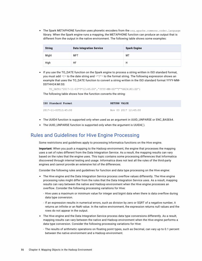
• The Spark METAPHONE function uses phonetic encoders from the org.apache.commons.codec.language library. When the Spark engine runs a mapping, the METAPHONE function can produce an output that is different from the output in the native environment. The following table shows some examples:
String Data Integration Service Spark Engine
Might MFT MT
High HF H
• If you use the TO_DATE function on the Spark engine to process a string written in ISO standard format, you must add *T* to the date string and *”T”* to the format string. The following expression shows an example that uses the TO_DATE function to convert a string written in the ISO standard format YYYY-MM-DDTHH24:MI:SS:
TO_DATE(‘2017-11-03*T*12:45:00’,’YYYY-MM-DD*”T”*HH24:MI:SS’)The following table shows how the function converts the string:
ISO Standard Format RETURN VALUE
2017-11-03T12:45:00 Nov 03 2017 12:45:00
• The UUID4 function is supported only when used as an argument in UUID_UNPARSE or ENC_BASE64.
• The UUID_UNPARSE function is supported only when the argument is UUID4( ).
Rules and Guidelines for Hive Engine ProcessingSome restrictions and guidelines apply to processing Informatica functions on the Hive engine.
Important: When you push a mapping to the Hadoop environment, the engine that processes the mapping uses a set of rules different from the Data Integration Service. As a result, the mapping results can vary based on the rules that the engine uses. This topic contains some processing differences that Informatica discovered through internal testing and usage. Informatica does not test all the rules of the third-party engines and cannot provide an extensive list of the differences.
Consider the following rules and guidelines for function and data type processing on the Hive engine:
• The Hive engine and the Data Integration Service process overflow values differently. The Hive engine processing rules might differ from the rules that the Data Integration Service uses. As a result, mapping results can vary between the native and Hadoop environment when the Hive engine processes an overflow. Consider the following processing variations for Hive:
- Hive uses a maximum or minimum value for integer and bigint data when there is data overflow during data type conversion.
- If an expression results in numerical errors, such as division by zero or SQRT of a negative number, it returns an infinite or an NaN value. In the native environment, the expression returns null values and the rows do not appear in the output.
• The Hive engine and the Data Integration Service process data type conversions differently. As a result, mapping results can vary between the native and Hadoop environment when the Hive engine performs a data type conversion. Consider the following processing variations for Hive:
- The results of arithmetic operations on floating point types, such as Decimal, can vary up to 0.1 percent between the native environment and a Hadoop environment.
86 Chapter 4: Mapping Objects in the Hadoop Environment
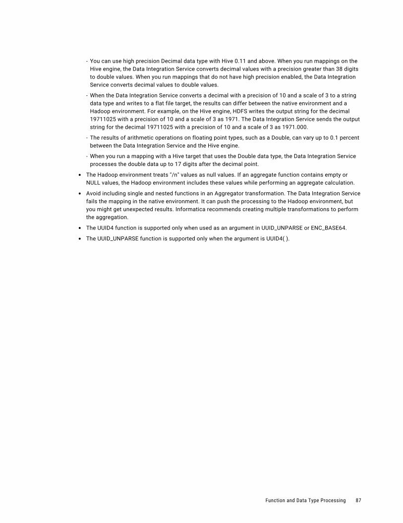
- You can use high precision Decimal data type with Hive 0.11 and above. When you run mappings on the Hive engine, the Data Integration Service converts decimal values with a precision greater than 38 digits to double values. When you run mappings that do not have high precision enabled, the Data Integration Service converts decimal values to double values.
- When the Data Integration Service converts a decimal with a precision of 10 and a scale of 3 to a string data type and writes to a flat file target, the results can differ between the native environment and a Hadoop environment. For example, on the Hive engine, HDFS writes the output string for the decimal 19711025 with a precision of 10 and a scale of 3 as 1971. The Data Integration Service sends the output string for the decimal 19711025 with a precision of 10 and a scale of 3 as 1971.000.
- The results of arithmetic operations on floating point types, such as a Double, can vary up to 0.1 percent between the Data Integration Service and the Hive engine.
- When you run a mapping with a Hive target that uses the Double data type, the Data Integration Service processes the double data up to 17 digits after the decimal point.
• The Hadoop environment treats "/n" values as null values. If an aggregate function contains empty or NULL values, the Hadoop environment includes these values while performing an aggregate calculation.
• Avoid including single and nested functions in an Aggregator transformation. The Data Integration Service fails the mapping in the native environment. It can push the processing to the Hadoop environment, but you might get unexpected results. Informatica recommends creating multiple transformations to perform the aggregation.
• The UUID4 function is supported only when used as an argument in UUID_UNPARSE or ENC_BASE64.
• The UUID_UNPARSE function is supported only when the argument is UUID4( ).
Function and Data Type Processing 87
C h a p t e r 5
Processing Hierarchical Data on the Spark Engine
This chapter includes the following topics:
• Processing Hierarchical Data on the Spark Engine Overview, 88
• How to Develop a Mapping to Process Hierarchical Data, 89
• Complex Data Types, 91
• Complex Ports, 96
• Complex Data Type Definitions, 98
• Type Configuration, 103
• Complex Operators, 107
• Complex Functions, 109
• Hierarchical Data Conversion, 110
Processing Hierarchical Data on the Spark Engine Overview
You can use complex data types, such as array, struct, and map, in mappings that run on the Spark engine. With complex data types, the Spark engine directly reads, processes, and writes hierarchical data in complex files.
The Spark engine can process hierarchical data in Avro, JSON, and Parquet complex files. The Spark engine uses complex data types to represent the native data types for hierarchical data in complex files. For example, a hierarchical data of type record in an Avro file is represented as a struct data type on the Spark engine.
You can develop mappings for the following hierarchical data processing scenarios:
• To generate and modify hierarchical data.
• To transform relational data to hierarchical data.
• To transform hierarchical data to relational data.
• To convert data from one complex file format to another. For example, read hierarchical data from an Avro source and write to a JSON target.
88
To read from and write to complex files, you create complex file data objects. Configure the read and write operations for the complex file data object to project columns as complex data types. Read and Write transformations based on these complex file data objects can read and write hierarchical data.
Configure the following objects and transformation properties in a mapping to process hierarchical data:
• Complex ports. To pass hierarchical data in a mapping, create complex ports. You create complex ports by assigning complex data types to ports.
• Complex data type definitions. To process hierarchical data of type struct, create or import complex data type definitions that represent the schema of struct data.
• Type configuration. To define the properties of a complex port, specify or change the type configuration.
• Complex operators and functions. To generate or modify hierarchical data, create expressions using complex operators and functions.
You can also use hierarchical conversion wizards to simplify some of the mapping development tasks.
How to Develop a Mapping to Process Hierarchical Data
Develop a mapping with complex ports, operators, and functions to process hierarchical data on the Spark engine.
Note: The tasks and the order in which you perform the tasks to develop the mapping depend on the mapping scenario.
The following list outlines the high-level tasks to develop and run a mapping to read, write, and process hierarchical data in complex files.
Create an HDFS connection.
Create a Hadoop Distributed File System (HDFS) connection to access data in complex files that are stored in the HDFS. You can create and manage an HDFS connection in the Administrator tool or the Developer tool.
Create a complex file data object.
1. Create a complex file data object to represent the complex files in the HDFS as sources or targets.The Developer tool creates the read and write operations when you create the complex file data object.
2. Configure the complex file data object properties.
3. In the read and write operations, enable the column file properties to project columns in the complex files as complex data types.
Create a mapping and add mapping objects.
1. Create a mapping, and add Read and Write transformations.To read from and write to a complex file, add Read and Write transformations based on the complex file data object.
To write to an Avro or Parquet file, you can also create a complex file target from an existing transformation in the mapping.
2. Based on the mapping logic, add other transformations that are supported on the Spark engine.
How to Develop a Mapping to Process Hierarchical Data 89
Generate struct data.
Based on the mapping scenario, use one of the hierarchical conversion wizards to generate struct data. You can also perform the following steps manually:Create or import complex data type definitions for struct ports.
1. Create or import complex data type definitions that represent the schema of the struct data.The complex data type definitions are stored in the type definition library, which is a Model repository object. The default name of the type definition library is Type_Definition_Library.
2. If a mapping uses one or more mapplets, rename the type definition libraries in the mapping and the mapplets to ensure that the names are unique.
Create and configure struct ports in transformations.
1. Create ports in transformations and assign struct complex data type.
2. Specify the type configuration for the struct ports.You must reference a complex data type definition for the struct port.
3. Create expressions with complex functions to generate struct data.
Modify struct data.
You can convert struct data to relational or hierarchical data. If the struct data contains elements of primitive data types, you can extract the elements as relational data. If the struct data contains elements of complex data types, you can extract the elements as hierarchical data. Based on the mapping scenario, use one of the hierarchical conversion wizards to modify struct data. You can also perform the following steps manually.
1. Create output ports with port properties that match the element of the struct data that you want to extract.
2. Create expressions with complex operators or complex functions to modify the struct data.
Generate array data.
1. Create ports in transformations and assign array complex data type.
2. Specify the type configuration for the array ports.
3. Create expressions with complex functions to generate array data.
Modify array data.
You can convert array data to relational or hierarchical data. If the array data contains elements of primitive data types, you can extract the elements as relational data. If the array data contains elements of complex data types, you can extract the elements as hierarchical data. Based on the mapping scenario, use one of the hierarchical conversion wizards to modify array data. You can also perform the following steps manually:
1. Create output ports with port properties that match the element of the array data that you want to extract.
2. Create expressions with complex operators or complex functions to modify the array data.
Configure the transformations.
Link the ports and configure the transformation properties based on the mapping logic.
Configure the mapping to run on the Spark engine.
Configure the following mapping run-time properties:
1. Select Hadoop as the validation environment and Spark as the engine.
2. Select Hadoop as the execution environment and select a Hadoop connection.
90 Chapter 5: Processing Hierarchical Data on the Spark Engine

Validate and run the mapping on the Spark engine.
1. Validate the mapping to fix any errors.
2. Optionally, view the Spark engine execution plan to debug the logic.
3. Run the mapping.
Complex Data TypesA complex data type is a transformation data type that represents multiple data values in a single column position. The data values are called elements. Elements in a complex data type can be of primitive or complex data types. Use complex data types to process hierarchical data in mappings that run on the Spark engine.
Transformation data types include the following data types:
Primitive data type
A transformation data type that represents a single data value in a single column position. Data types such as decimal, integer, and string are primitive data types. You can assign primitive data types to ports in any transformation.
Complex data type
A transformation data type that represents multiple data values in a single column position. Data types such as array, map, and struct are complex data types. You can assign complex data types to ports in some transformations for the Spark engine.
Nested data type
A complex data type that contains elements of complex data types. Complex data types such as an array of structs or a struct with an array of other structs are nested data types.
The following table lists the complex data types:
Complex Data Type
Description
array An array is an ordered collection of elements.The elements can be of a primitive or complex data type. All elements in the array must be of the same data type.
map A map is an unordered collection of key-value pair elements.The key must be of a primitive data type. The value can be of a primitive or complex data type.Note: The Spark engine can read, pass through, and write map data but cannot generate or process map data.
struct A struct is a collection of elements of different data types.The elements can be of primitive or complex data types. Struct has a schema that defines the structure of the data.
Complex Data Types 91
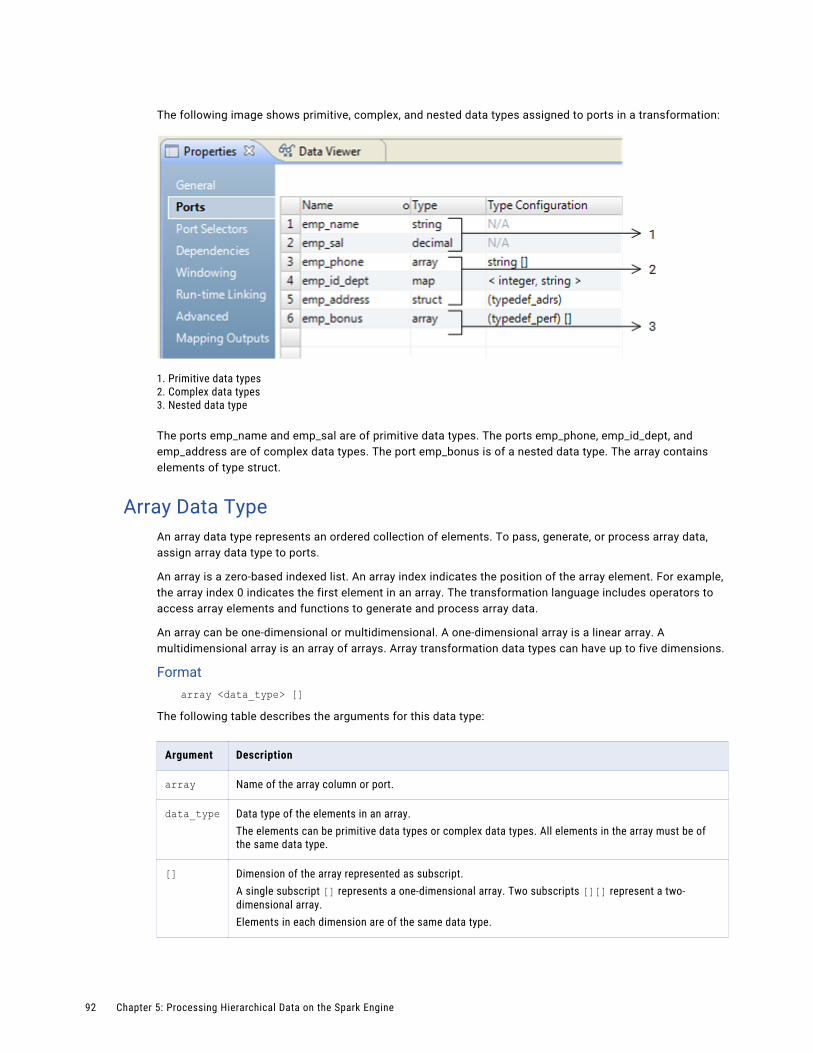
The following image shows primitive, complex, and nested data types assigned to ports in a transformation:
1. Primitive data types2. Complex data types3. Nested data type
The ports emp_name and emp_sal are of primitive data types. The ports emp_phone, emp_id_dept, and emp_address are of complex data types. The port emp_bonus is of a nested data type. The array contains elements of type struct.
Array Data TypeAn array data type represents an ordered collection of elements. To pass, generate, or process array data, assign array data type to ports.
An array is a zero-based indexed list. An array index indicates the position of the array element. For example, the array index 0 indicates the first element in an array. The transformation language includes operators to access array elements and functions to generate and process array data.
An array can be one-dimensional or multidimensional. A one-dimensional array is a linear array. A multidimensional array is an array of arrays. Array transformation data types can have up to five dimensions.
Formatarray <data_type> []
The following table describes the arguments for this data type:
Argument Description
array Name of the array column or port.
data_type Data type of the elements in an array.The elements can be primitive data types or complex data types. All elements in the array must be of the same data type.
[] Dimension of the array represented as subscript.A single subscript [] represents a one-dimensional array. Two subscripts [][] represent a two-dimensional array.Elements in each dimension are of the same data type.
92 Chapter 5: Processing Hierarchical Data on the Spark Engine

The elements of an array do not have names. The number of elements in an array can be different for each row.
Array Examples
One-dimensional array
The following array column represents a one-dimensional array of string elements that contains customer phone numbers:
custphone string[]The following example shows data values for the custphone column:
custphone
[205-128-6478,722-515-2889]
[107-081-0961,718-051-8116]
[107-031-0961,NULL]
Two-dimensional array
The following array column represents a two-dimensional array of string elements that contains customer work and personal email addresses.
email_work_pers string[][]The following example shows data values for the email_work_pers column:
email_work_pers
[[email protected],[email protected]][[email protected],[email protected]]
[[email protected],[email protected]][[email protected],[email protected]]
[[email protected],[email protected]][[email protected],NULL]
Map Data TypeA map data type represents an unordered collection of key-value pair elements. To pass map data through transformations, assign map data type to ports.
A map element is a key and value pair that maps one thing to another. The Spark engine can read and write map data in complex files, and pass through map data in a mapping.
Formatmap <primitive_type, data_type>
Complex Data Types 93
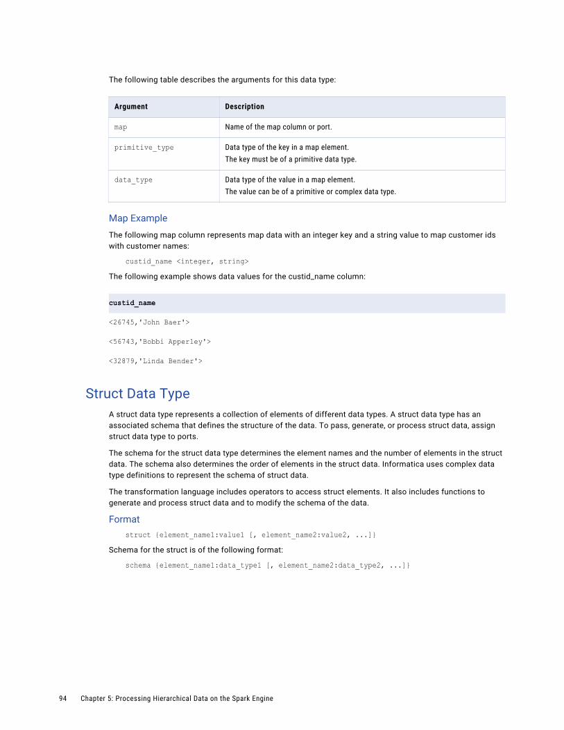
The following table describes the arguments for this data type:
Argument Description
map Name of the map column or port.
primitive_type Data type of the key in a map element.The key must be of a primitive data type.
data_type Data type of the value in a map element.The value can be of a primitive or complex data type.
Map Example
The following map column represents map data with an integer key and a string value to map customer ids with customer names:
custid_name <integer, string>The following example shows data values for the custid_name column:
custid_name
<26745,'John Baer'>
<56743,'Bobbi Apperley'>
<32879,'Linda Bender'>
Struct Data TypeA struct data type represents a collection of elements of different data types. A struct data type has an associated schema that defines the structure of the data. To pass, generate, or process struct data, assign struct data type to ports.
The schema for the struct data type determines the element names and the number of elements in the struct data. The schema also determines the order of elements in the struct data. Informatica uses complex data type definitions to represent the schema of struct data.
The transformation language includes operators to access struct elements. It also includes functions to generate and process struct data and to modify the schema of the data.
Formatstruct {element_name1:value1 [, element_name2:value2, ...]}
Schema for the struct is of the following format:
schema {element_name1:data_type1 [, element_name2:data_type2, ...]}
94 Chapter 5: Processing Hierarchical Data on the Spark Engine
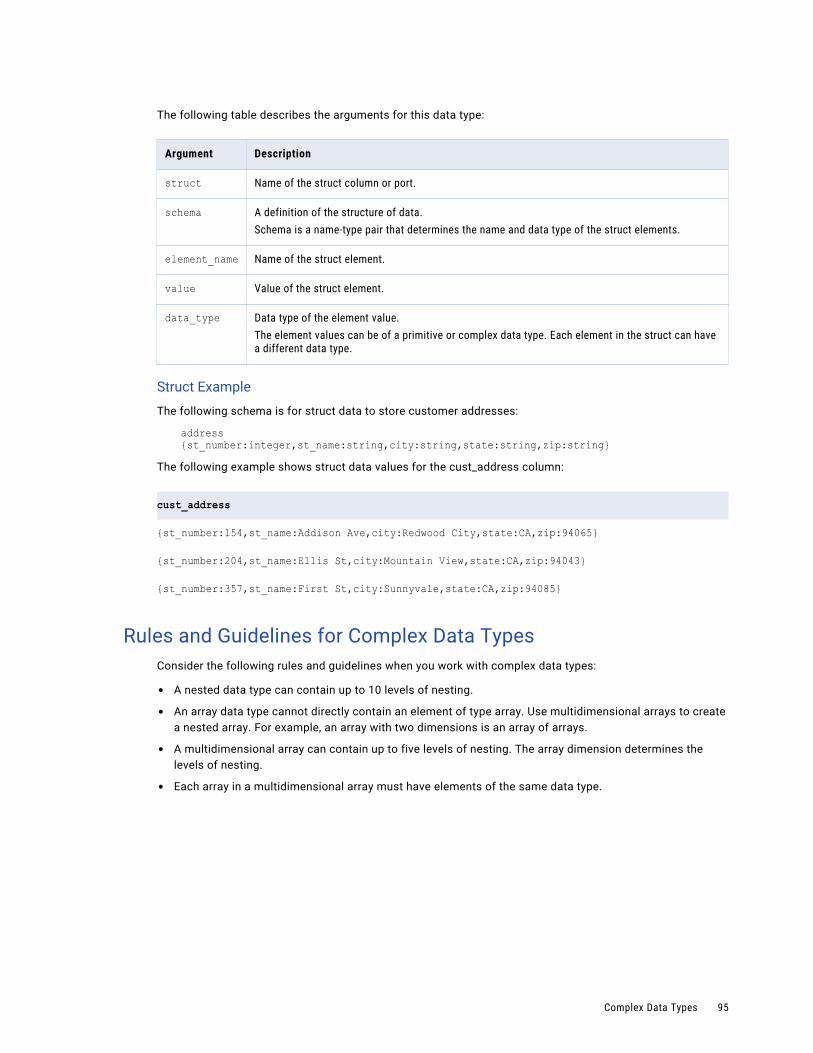
The following table describes the arguments for this data type:
Argument Description
struct Name of the struct column or port.
schema A definition of the structure of data.Schema is a name-type pair that determines the name and data type of the struct elements.
element_name Name of the struct element.
value Value of the struct element.
data_type Data type of the element value.The element values can be of a primitive or complex data type. Each element in the struct can have a different data type.
Struct Example
The following schema is for struct data to store customer addresses:
address {st_number:integer,st_name:string,city:string,state:string,zip:string}
The following example shows struct data values for the cust_address column:
cust_address
{st_number:154,st_name:Addison Ave,city:Redwood City,state:CA,zip:94065}
{st_number:204,st_name:Ellis St,city:Mountain View,state:CA,zip:94043}
{st_number:357,st_name:First St,city:Sunnyvale,state:CA,zip:94085}
Rules and Guidelines for Complex Data TypesConsider the following rules and guidelines when you work with complex data types:
• A nested data type can contain up to 10 levels of nesting.
• An array data type cannot directly contain an element of type array. Use multidimensional arrays to create a nested array. For example, an array with two dimensions is an array of arrays.
• A multidimensional array can contain up to five levels of nesting. The array dimension determines the levels of nesting.
• Each array in a multidimensional array must have elements of the same data type.
Complex Data Types 95
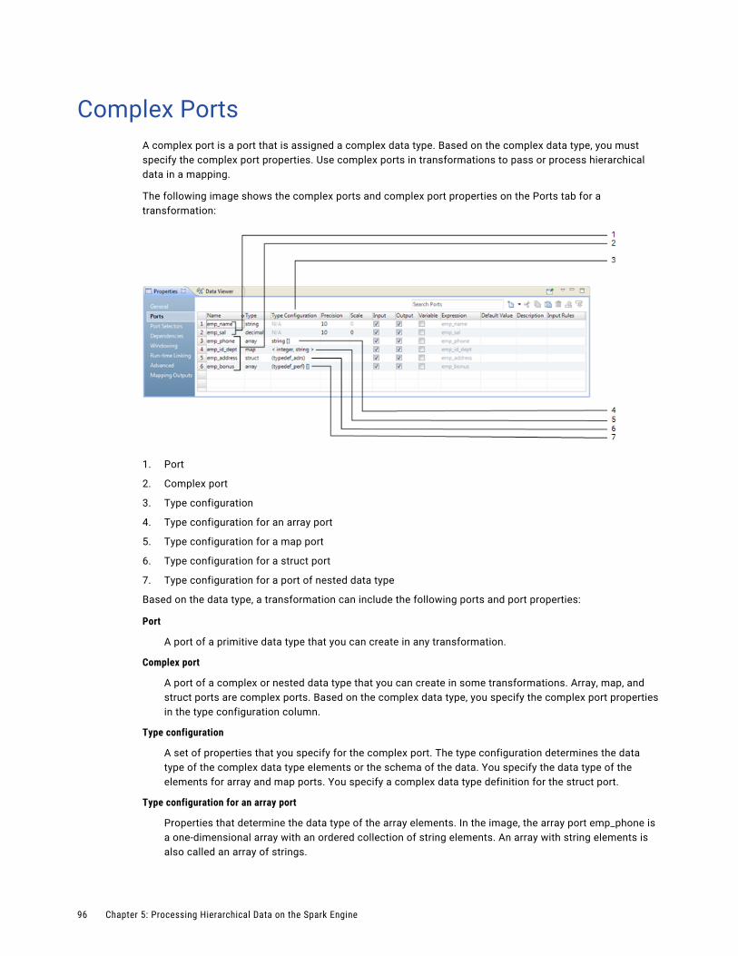
Complex PortsA complex port is a port that is assigned a complex data type. Based on the complex data type, you must specify the complex port properties. Use complex ports in transformations to pass or process hierarchical data in a mapping.
The following image shows the complex ports and complex port properties on the Ports tab for a transformation:
1. Port
2. Complex port
3. Type configuration
4. Type configuration for an array port
5. Type configuration for a map port
6. Type configuration for a struct port
7. Type configuration for a port of nested data type
Based on the data type, a transformation can include the following ports and port properties:
Port
A port of a primitive data type that you can create in any transformation.
Complex port
A port of a complex or nested data type that you can create in some transformations. Array, map, and struct ports are complex ports. Based on the complex data type, you specify the complex port properties in the type configuration column.
Type configuration
A set of properties that you specify for the complex port. The type configuration determines the data type of the complex data type elements or the schema of the data. You specify the data type of the elements for array and map ports. You specify a complex data type definition for the struct port.
Type configuration for an array port
Properties that determine the data type of the array elements. In the image, the array port emp_phone is a one-dimensional array with an ordered collection of string elements. An array with string elements is also called an array of strings.
96 Chapter 5: Processing Hierarchical Data on the Spark Engine
Type configuration for a map port
Properties that determine the data type of the key-value pair of the map elements. In the image, the map port emp_id_dept is an unordered collection of key-value pairs of type integer and string.
Type configuration for a struct port
Properties that determine the schema of the data. To represent the schema, you create or import a complex data type definition. In the image, the struct port emp_address references a complex data type definition typedef_adrs.
Type configuration for a port of nested data type
Properties that determine the nested data type. In the image, the array port emp_bonus is a one-dimensional array with an ordered collection of struct elements. The struct elements reference a complex data type definition typedef_bonus. An array with struct elements is also called an array of structs.
Complex Ports in TransformationsYou can create complex ports in some transformations that are supported on the Spark engine. Read and Write transformations can represent ports that pass hierarchical data as complex data types.
You can create complex ports in the following transformations:
• Aggregator
• Expression
• Filter
• Joiner
• Lookup
• Normalizer
• Router
• Sorter
• Union
The Read and Write transformations can read and write hierarchical data in complex files. To read and write hierarchical data, the Read and Write transformations must meet the following requirements:
• The transformation must be based on a complex file data object.
• The data object read and write operations must project columns as complex data types.
Rules and Guidelines for Complex PortsConsider the following rules and guidelines when you work with complex ports:
• Aggregator transformation. You cannot define a group by value as a complex port.
• Filter transformation. You cannot use the operators >, < , >=, and <= in a filter condition to compare data in complex ports.
• Joiner transformation. You cannot use the operators >, < , >=, and <= in a join condition to compare data in complex ports.
• Lookup transformation. You cannot use a complex port in a lookup condition.
• Rank transformation. You cannot define a group by or rank value as a complex port.
Complex Ports 97
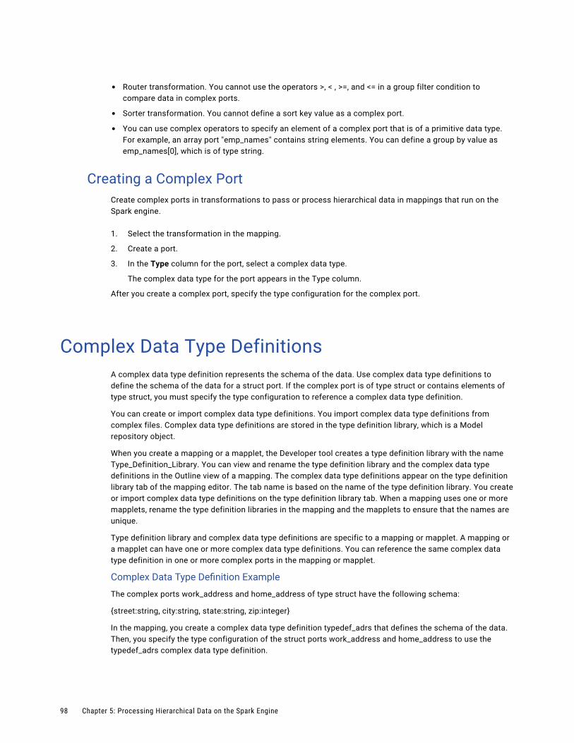
• Router transformation. You cannot use the operators >, < , >=, and <= in a group filter condition to compare data in complex ports.
• Sorter transformation. You cannot define a sort key value as a complex port.
• You can use complex operators to specify an element of a complex port that is of a primitive data type.For example, an array port "emp_names" contains string elements. You can define a group by value as emp_names[0], which is of type string.
Creating a Complex PortCreate complex ports in transformations to pass or process hierarchical data in mappings that run on the Spark engine.
1. Select the transformation in the mapping.
2. Create a port.
3. In the Type column for the port, select a complex data type.
The complex data type for the port appears in the Type column.
After you create a complex port, specify the type configuration for the complex port.
Complex Data Type DefinitionsA complex data type definition represents the schema of the data. Use complex data type definitions to define the schema of the data for a struct port. If the complex port is of type struct or contains elements of type struct, you must specify the type configuration to reference a complex data type definition.
You can create or import complex data type definitions. You import complex data type definitions from complex files. Complex data type definitions are stored in the type definition library, which is a Model repository object.
When you create a mapping or a mapplet, the Developer tool creates a type definition library with the name Type_Definition_Library. You can view and rename the type definition library and the complex data type definitions in the Outline view of a mapping. The complex data type definitions appear on the type definition library tab of the mapping editor. The tab name is based on the name of the type definition library. You create or import complex data type definitions on the type definition library tab. When a mapping uses one or more mapplets, rename the type definition libraries in the mapping and the mapplets to ensure that the names are unique.
Type definition library and complex data type definitions are specific to a mapping or mapplet. A mapping or a mapplet can have one or more complex data type definitions. You can reference the same complex data type definition in one or more complex ports in the mapping or mapplet.
Complex Data Type Definition Example
The complex ports work_address and home_address of type struct have the following schema:
{street:string, city:string, state:string, zip:integer}
In the mapping, you create a complex data type definition typedef_adrs that defines the schema of the data. Then, you specify the type configuration of the struct ports work_address and home_address to use the typedef_adrs complex data type definition.
98 Chapter 5: Processing Hierarchical Data on the Spark Engine
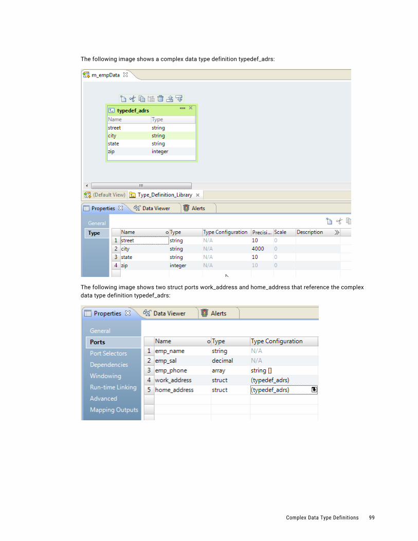
The following image shows a complex data type definition typedef_adrs:
The following image shows two struct ports work_address and home_address that reference the complex data type definition typedef_adrs:
Complex Data Type Definitions 99
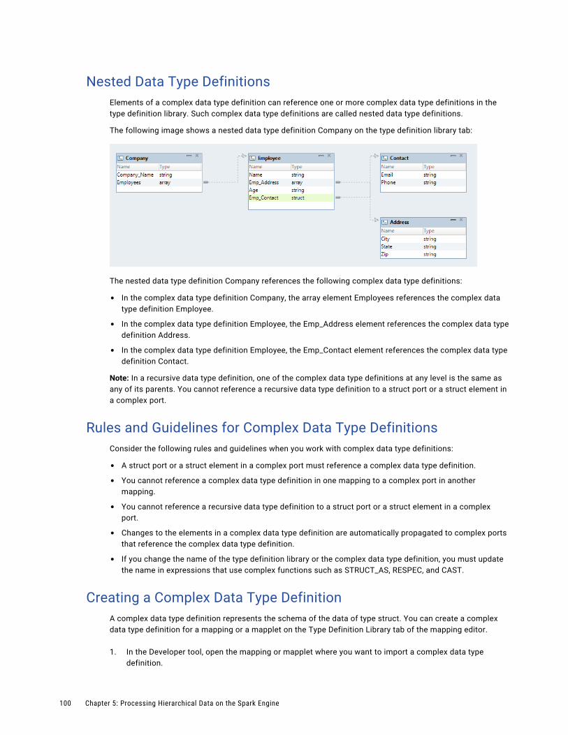
Nested Data Type DefinitionsElements of a complex data type definition can reference one or more complex data type definitions in the type definition library. Such complex data type definitions are called nested data type definitions.
The following image shows a nested data type definition Company on the type definition library tab:
The nested data type definition Company references the following complex data type definitions:
• In the complex data type definition Company, the array element Employees references the complex data type definition Employee.
• In the complex data type definition Employee, the Emp_Address element references the complex data type definition Address.
• In the complex data type definition Employee, the Emp_Contact element references the complex data type definition Contact.
Note: In a recursive data type definition, one of the complex data type definitions at any level is the same as any of its parents. You cannot reference a recursive data type definition to a struct port or a struct element in a complex port.
Rules and Guidelines for Complex Data Type DefinitionsConsider the following rules and guidelines when you work with complex data type definitions:
• A struct port or a struct element in a complex port must reference a complex data type definition.
• You cannot reference a complex data type definition in one mapping to a complex port in another mapping.
• You cannot reference a recursive data type definition to a struct port or a struct element in a complex port.
• Changes to the elements in a complex data type definition are automatically propagated to complex ports that reference the complex data type definition.
• If you change the name of the type definition library or the complex data type definition, you must update the name in expressions that use complex functions such as STRUCT_AS, RESPEC, and CAST.
Creating a Complex Data Type DefinitionA complex data type definition represents the schema of the data of type struct. You can create a complex data type definition for a mapping or a mapplet on the Type Definition Library tab of the mapping editor.
1. In the Developer tool, open the mapping or mapplet where you want to import a complex data type definition.
100 Chapter 5: Processing Hierarchical Data on the Spark Engine
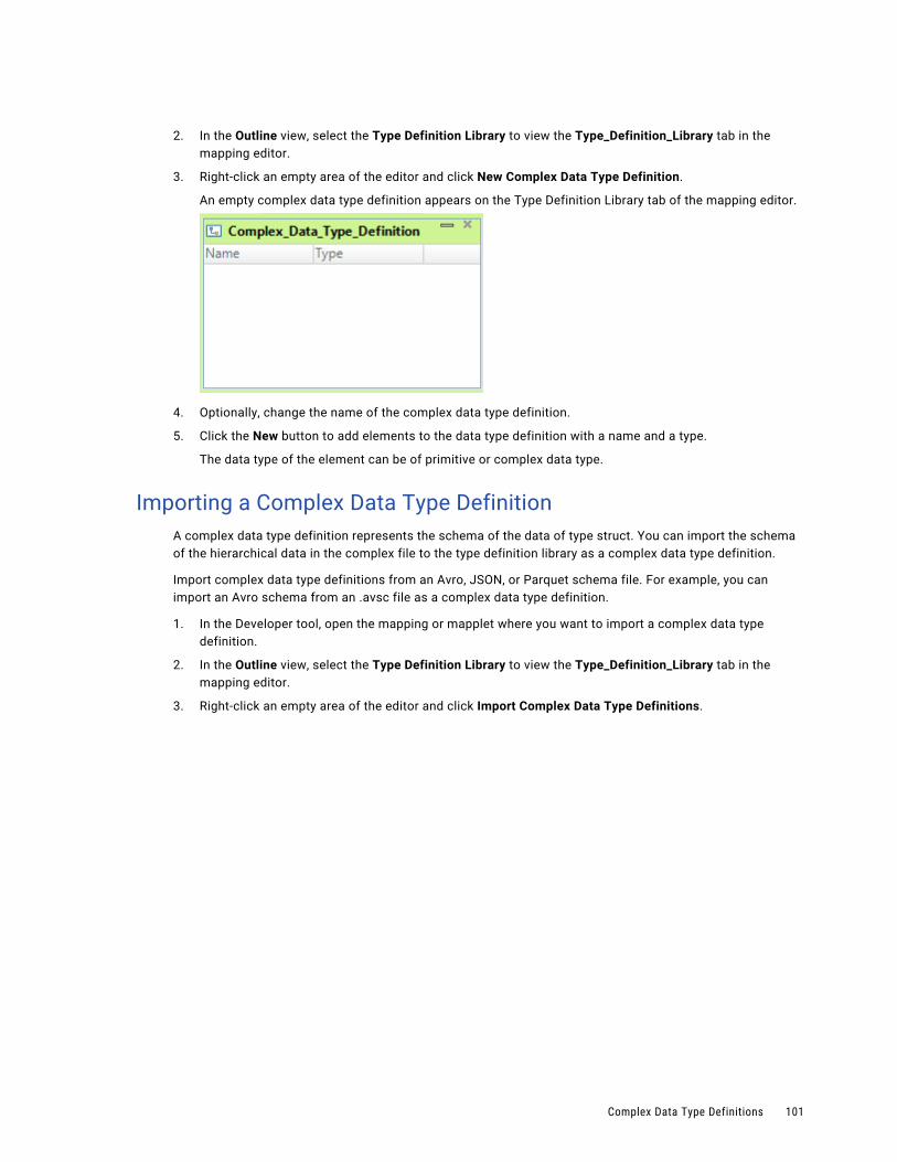
2. In the Outline view, select the Type Definition Library to view the Type_Definition_Library tab in the mapping editor.
3. Right-click an empty area of the editor and click New Complex Data Type Definition.
An empty complex data type definition appears on the Type Definition Library tab of the mapping editor.
4. Optionally, change the name of the complex data type definition.
5. Click the New button to add elements to the data type definition with a name and a type.
The data type of the element can be of primitive or complex data type.
Importing a Complex Data Type DefinitionA complex data type definition represents the schema of the data of type struct. You can import the schema of the hierarchical data in the complex file to the type definition library as a complex data type definition.
Import complex data type definitions from an Avro, JSON, or Parquet schema file. For example, you can import an Avro schema from an .avsc file as a complex data type definition.
1. In the Developer tool, open the mapping or mapplet where you want to import a complex data type definition.
2. In the Outline view, select the Type Definition Library to view the Type_Definition_Library tab in the mapping editor.
3. Right-click an empty area of the editor and click Import Complex Data Type Definitions.
Complex Data Type Definitions 101
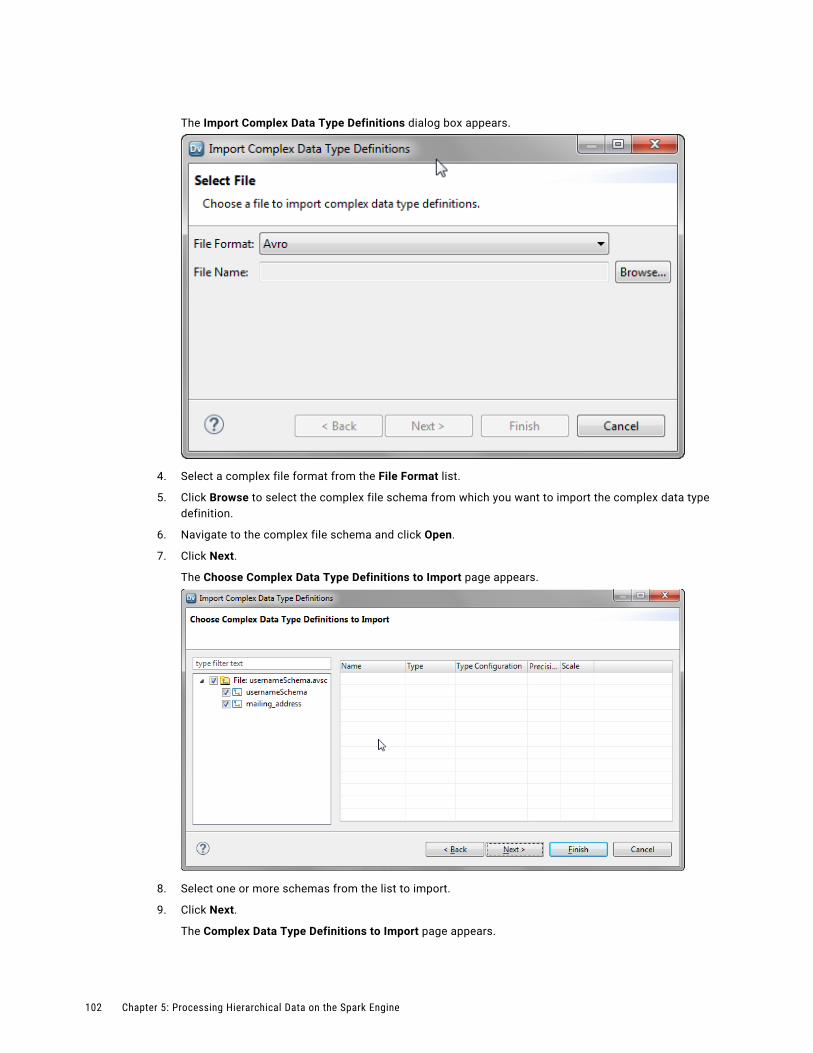
The Import Complex Data Type Definitions dialog box appears.
4. Select a complex file format from the File Format list.
5. Click Browse to select the complex file schema from which you want to import the complex data type definition.
6. Navigate to the complex file schema and click Open.
7. Click Next.
The Choose Complex Data Type Definitions to Import page appears.
8. Select one or more schemas from the list to import.
9. Click Next.
The Complex Data Type Definitions to Import page appears.
102 Chapter 5: Processing Hierarchical Data on the Spark Engine
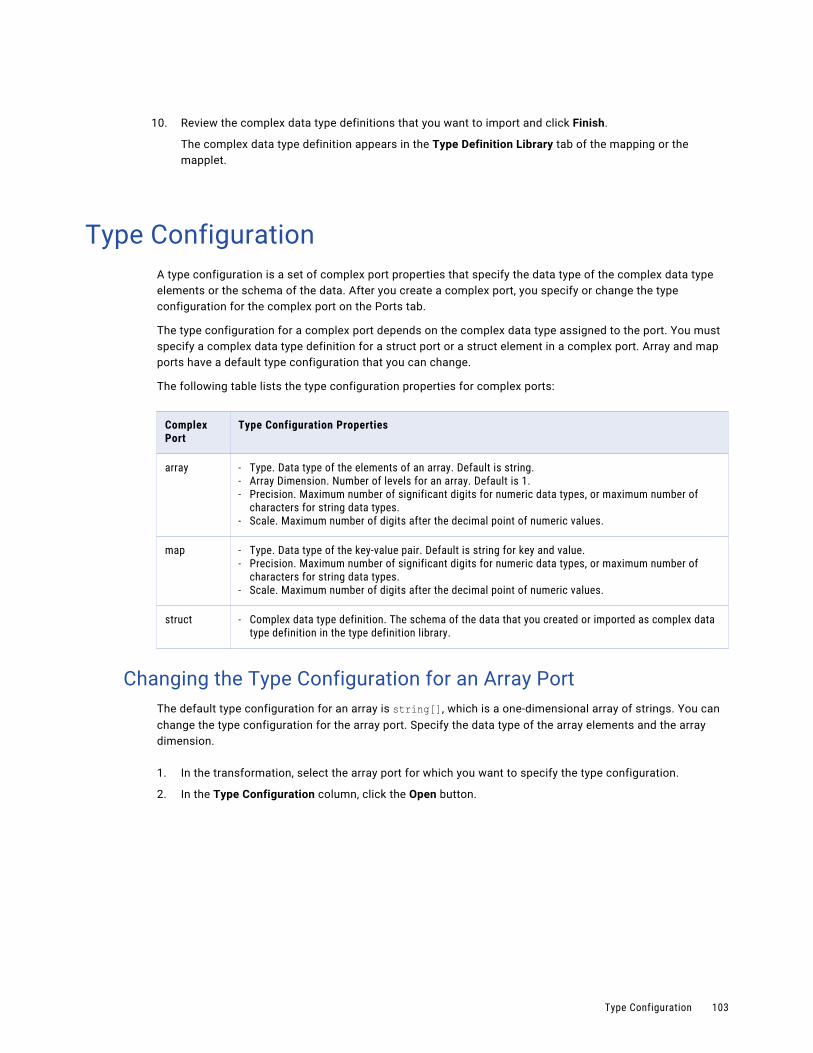
10. Review the complex data type definitions that you want to import and click Finish.
The complex data type definition appears in the Type Definition Library tab of the mapping or the mapplet.
Type ConfigurationA type configuration is a set of complex port properties that specify the data type of the complex data type elements or the schema of the data. After you create a complex port, you specify or change the type configuration for the complex port on the Ports tab.
The type configuration for a complex port depends on the complex data type assigned to the port. You must specify a complex data type definition for a struct port or a struct element in a complex port. Array and map ports have a default type configuration that you can change.
The following table lists the type configuration properties for complex ports:
Complex Port
Type Configuration Properties
array - Type. Data type of the elements of an array. Default is string.- Array Dimension. Number of levels for an array. Default is 1.- Precision. Maximum number of significant digits for numeric data types, or maximum number of
characters for string data types.- Scale. Maximum number of digits after the decimal point of numeric values.
map - Type. Data type of the key-value pair. Default is string for key and value.- Precision. Maximum number of significant digits for numeric data types, or maximum number of
characters for string data types.- Scale. Maximum number of digits after the decimal point of numeric values.
struct - Complex data type definition. The schema of the data that you created or imported as complex data type definition in the type definition library.
Changing the Type Configuration for an Array PortThe default type configuration for an array is string[], which is a one-dimensional array of strings. You can change the type configuration for the array port. Specify the data type of the array elements and the array dimension.
1. In the transformation, select the array port for which you want to specify the type configuration.
2. In the Type Configuration column, click the Open button.
Type Configuration 103
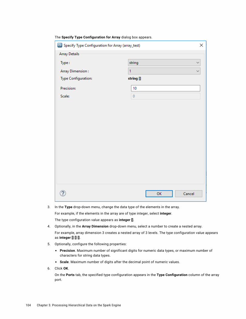
The Specify Type Configuration for Array dialog box appears.
3. In the Type drop-down menu, change the data type of the elements in the array.
For example, if the elements in the array are of type integer, select integer.
The type configuration value appears as integer [].
4. Optionally, in the Array Dimension drop-down menu, select a number to create a nested array.
For example, array dimension 3 creates a nested array of 3 levels. The type configuration value appears as integer [] [] [].
5. Optionally, configure the following properties:
• Precision. Maximum number of significant digits for numeric data types, or maximum number of characters for string data types.
• Scale. Maximum number of digits after the decimal point of numeric values.
6. Click OK.
On the Ports tab, the specified type configuration appears in the Type Configuration column of the array port.
104 Chapter 5: Processing Hierarchical Data on the Spark Engine

Changing the Type Configuration for a Map PortThe default type configuration for a map is <string, string>. You can change the type configuration for a map port. Specify the data type of the key-value pair.
1. In the transformation, select the map port for which you want to set the type configuration.
2. In the Type Configuration column, click the Open button.
The Type Configuration dialog box appears:
3. Specify the properties for the key and value of the map data type.
a. In the Type drop-down menu, select the data type.
b. Optionally, in the Precision box, specify the maximum number of significant digits for numeric data types, or maximum number of characters for string data types.
c. Optionally, in the Scale box, specify the maximum number of digits after the decimal point of numeric values.
4. Click OK.
On the Ports tab, the specified type configuration appears in the Type Configuration column of the map port.
Type Configuration 105
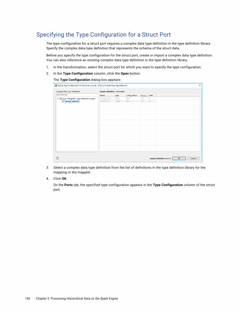
Specifying the Type Configuration for a Struct PortThe type configuration for a struct port requires a complex data type definition in the type definition library. Specify the complex data type definition that represents the schema of the struct data.
Before you specify the type configuration for the struct port, create or import a complex data type definition. You can also reference an existing complex data type definition in the type definition library.
1. In the transformation, select the struct port for which you want to specify the type configuration.
2. In the Type Configuration column, click the Open button.
The Type Configuration dialog box appears:
3. Select a complex data type definition from the list of definitions in the type definition library for the mapping or the mapplet.
4. Click OK.
On the Ports tab, the specified type configuration appears in the Type Configuration column of the struct port.
106 Chapter 5: Processing Hierarchical Data on the Spark Engine

Complex OperatorsA complex operator is a type of operator to access elements in a complex data type. The transformation language includes complex operators for array and struct data types. Use complex operators to access or extract elements in hierarchical data.
The following table lists the complex operators:
Complex Operators Description
[] Subscript operator.Syntax: array[index]- array is the array from which you want to access an element.- index is the position of an element within an array.For example, use [0] to access the first element in an one-dimensional array.
. Dot operator.Syntax: struct.element_name- struct is the struct from which you want to access an element.- element_name is the name of the struct element.
Use complex operators in expressions to convert hierarchical data to relational data.
For more information about the operator syntax, return values, and examples, see the Informatica Developer Transformation Language Reference.
Complex Operator Examples• Convert array data in a JSON file to relational data.
A JSON file has a quarterly_sales column that is of the array type with integer elements. You develop a mapping to transform the hierarchical data to relational data. The array port quarterly_sales contains four elements. Use subscript operators in expressions to extract the four elements into the four integer ports, q1_sales, q2_sales, q3_sales, and q4_sales.
The expressions for the integer output port are as follows:
quarterly_sales[0]quarterly_sales[1]quarterly_sales[2]quarterly_sales[3]
• Convert struct data in a Parquet file to relational data.A Parquet file has an address column that contains customer address as a struct type. You develop a mapping to transform hierarchical data to relational data. The struct port address contains three elements city, state, and zip, of type string. Use dot operators in expressions to extract the three struct elements into the three string ports, city, state, and zip.
The expressions for the string output port are as follows:
address.cityaddress.stateaddress.zip
Complex Operators 107
Extracting an Array Element Using a Subscript OperatorUse the subscript operator in expressions to extract one or more elements of an array.
1. In the transformation, create an output port of the same data type as the return value of the array element that you want to extract.
To extract more than one element in an array, create an array output port. The data type of the elements in the type configuration for the array port must match the data type of the return value of the array elements.
2. In the Expression column for the output port, click the Open button.
The Expression Editor opens.
3. Delete the existing expression in the editor.
4. Click the Ports tab and select an array port.
5. Enter one or more index values within the subscript operator.
To extract array elements in a multidimensional array, enter index values within each subscript operator.
6. Click Validate to validate the expression.
7. Click OK to exit the Validate Expression dialog box.
8. Click OK to exit the Expression Editor.
Extracting a Struct Element Using the Dot OperatorUse the dot operator in expressions to extract elements of a struct.
1. In the transformation, create an output port of the same data type as the return value of the struct element that you want to extract.
2. In the Expression column for the output port, click the Open button.
The Expression Editor opens.
3. Delete the existing expression in the editor.
4. Click the Ports tab and select the struct port.
5. Enter a dot after the port name.
108 Chapter 5: Processing Hierarchical Data on the Spark Engine
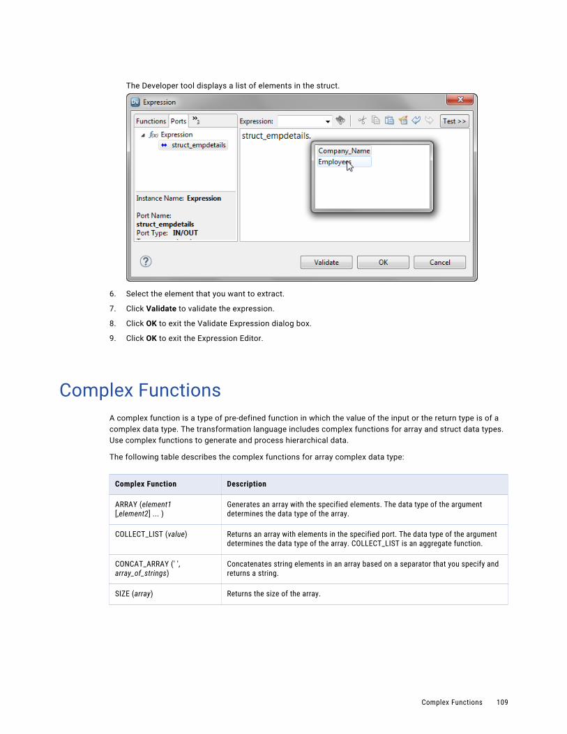
The Developer tool displays a list of elements in the struct.
6. Select the element that you want to extract.
7. Click Validate to validate the expression.
8. Click OK to exit the Validate Expression dialog box.
9. Click OK to exit the Expression Editor.
Complex FunctionsA complex function is a type of pre-defined function in which the value of the input or the return type is of a complex data type. The transformation language includes complex functions for array and struct data types. Use complex functions to generate and process hierarchical data.
The following table describes the complex functions for array complex data type:
Complex Function Description
ARRAY (element1 [,element2] ... )
Generates an array with the specified elements. The data type of the argument determines the data type of the array.
COLLECT_LIST (value) Returns an array with elements in the specified port. The data type of the argument determines the data type of the array. COLLECT_LIST is an aggregate function.
CONCAT_ARRAY (' ', array_of_strings)
Concatenates string elements in an array based on a separator that you specify and returns a string.
SIZE (array) Returns the size of the array.
Complex Functions 109
The following table describes the complex functions for struct complex data type:
Complex Function Description
STRUCT_AS (type_definition, struct)
Generates a struct with a schema based on the specified complex data type definition and the values you pass as argument.
STRUCT (element_name1, value1)
Generates a struct with the specified names and values for the elements. The data type of the value is based on the specified value argument.
RESPEC (type_definition, struct)
Renames each element of the given struct value based on the names of the elements in the specified complex data type definition.
CAST (type_definition, struct)
Changes the data type and the name of each element for the given struct value based on the corresponding data type and name of the element in the specified complex data type definition.
For more information about the function syntax, return value, and examples, see the Informatica Developer Transformation Language Reference.
Hierarchical Data ConversionIn the Developer tool, use Hierarchical Conversion wizards that simplify the tasks for developing a mapping to process hierarchical data on the Spark engine. These wizards add one or more transformations to the mapping and create output ports. The expressions in the output ports use complex functions and operators to convert relational data to hierarchical data or hierarchical data to relational data.
The following table lists the hierarchical conversion wizards and when to use these wizards:
Hierarchical Conversion Wizard
When to Use
Create Struct Port To convert relational and hierarchical data to struct data. For example, you want to convert data in one or more columns of any data type to hierarchical data column of type struct.
Create Nested Complex Port
To convert relational and hierarchical data in two tables to a nested struct data. You can select one or more columns of any data type. For example, you want to convert data in columns from two tables to a hierarchical data column of type struct with a nested schema. The wizard creates a struct with an array of structs.
Extract from Complex Port
To convert hierarchical data to relational data or modify the hierarchical data. For example, you want to perform the following conversions:- Convert one or more elements of primitive data types in a hierarchical data to relational data
columns.- Convert one or more elements of complex data types in a hierarchical data to hierarchical
data columns.
Flatten Complex Port
To convert hierarchical data to relational data. For example, you want to convert one or more elements of a hierarchical data to relational data columns.
110 Chapter 5: Processing Hierarchical Data on the Spark Engine
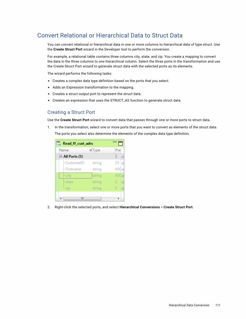
Convert Relational or Hierarchical Data to Struct DataYou can convert relational or hierarchical data in one or more columns to hierarchical data of type struct. Use the Create Struct Port wizard in the Developer tool to perform the conversion.
For example, a relational table contains three columns city, state, and zip. You create a mapping to convert the data in the three columns to one hierarchical column. Select the three ports in the transformation and use the Create Struct Port wizard to generate struct data with the selected ports as its elements.
The wizard performs the following tasks:
• Creates a complex data type definition based on the ports that you select.
• Adds an Expression transformation to the mapping.
• Creates a struct output port to represent the struct data.
• Creates an expression that uses the STRUCT_AS function to generate struct data.
Creating a Struct PortUse the Create Struct Port wizard to convert data that passes through one or more ports to struct data.
1. In the transformation, select one or more ports that you want to convert as elements of the struct data.
The ports you select also determine the elements of the complex data type definition.
2. Right-click the selected ports, and select Hierarchical Conversions > Create Struct Port.
Hierarchical Data Conversion 111
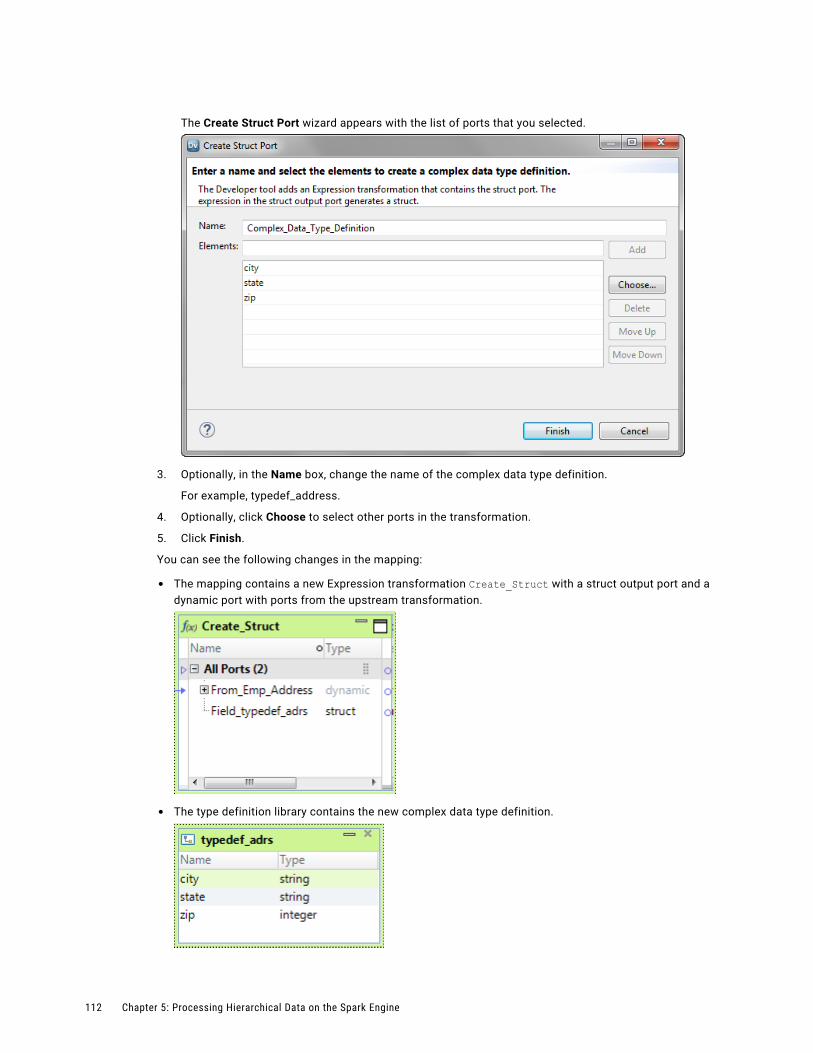
The Create Struct Port wizard appears with the list of ports that you selected.
3. Optionally, in the Name box, change the name of the complex data type definition.
For example, typedef_address.
4. Optionally, click Choose to select other ports in the transformation.
5. Click Finish.
You can see the following changes in the mapping:
• The mapping contains a new Expression transformation Create_Struct with a struct output port and a dynamic port with ports from the upstream transformation.
• The type definition library contains the new complex data type definition.
112 Chapter 5: Processing Hierarchical Data on the Spark Engine
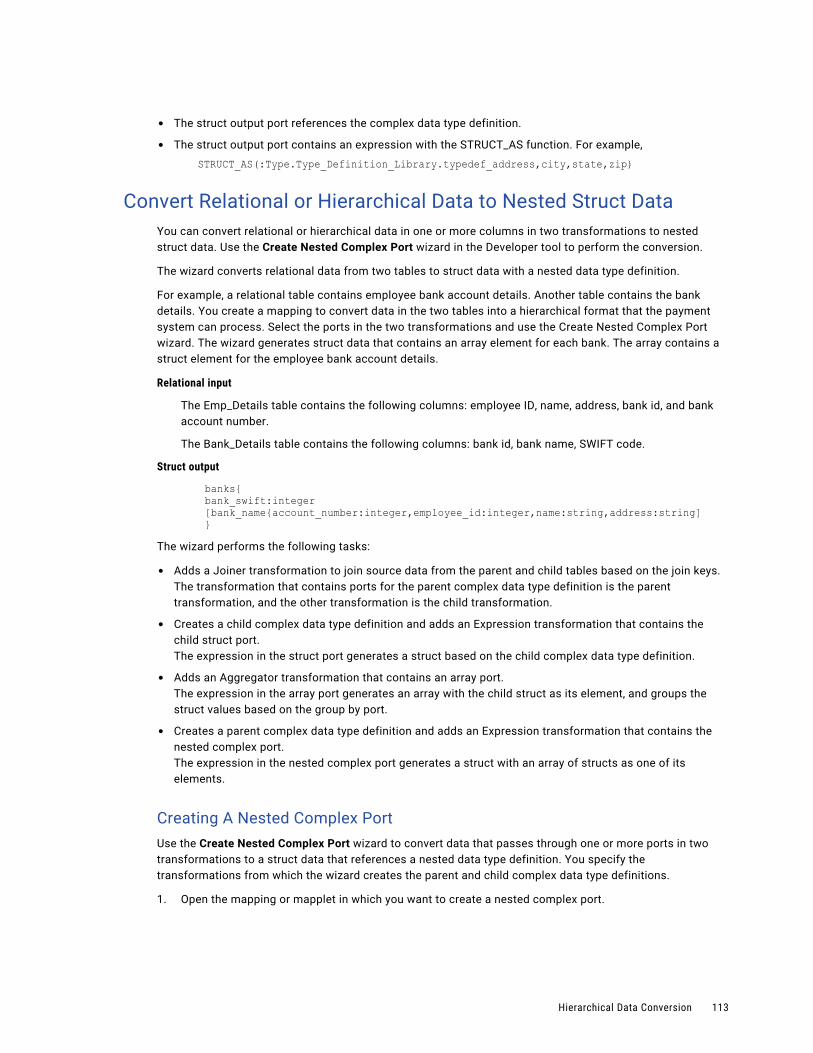
• The struct output port references the complex data type definition.
• The struct output port contains an expression with the STRUCT_AS function. For example,
STRUCT_AS(:Type.Type_Definition_Library.typedef_address,city,state,zip)
Convert Relational or Hierarchical Data to Nested Struct DataYou can convert relational or hierarchical data in one or more columns in two transformations to nested struct data. Use the Create Nested Complex Port wizard in the Developer tool to perform the conversion.
The wizard converts relational data from two tables to struct data with a nested data type definition.
For example, a relational table contains employee bank account details. Another table contains the bank details. You create a mapping to convert data in the two tables into a hierarchical format that the payment system can process. Select the ports in the two transformations and use the Create Nested Complex Port wizard. The wizard generates struct data that contains an array element for each bank. The array contains a struct element for the employee bank account details.
Relational input
The Emp_Details table contains the following columns: employee ID, name, address, bank id, and bank account number.
The Bank_Details table contains the following columns: bank id, bank name, SWIFT code.
Struct output
banks{bank_swift:integer[bank_name{account_number:integer,employee_id:integer,name:string,address:string]}
The wizard performs the following tasks:
• Adds a Joiner transformation to join source data from the parent and child tables based on the join keys.The transformation that contains ports for the parent complex data type definition is the parent transformation, and the other transformation is the child transformation.
• Creates a child complex data type definition and adds an Expression transformation that contains the child struct port.The expression in the struct port generates a struct based on the child complex data type definition.
• Adds an Aggregator transformation that contains an array port.The expression in the array port generates an array with the child struct as its element, and groups the struct values based on the group by port.
• Creates a parent complex data type definition and adds an Expression transformation that contains the nested complex port.The expression in the nested complex port generates a struct with an array of structs as one of its elements.
Creating A Nested Complex PortUse the Create Nested Complex Port wizard to convert data that passes through one or more ports in two transformations to a struct data that references a nested data type definition. You specify the transformations from which the wizard creates the parent and child complex data type definitions.
1. Open the mapping or mapplet in which you want to create a nested complex port.
Hierarchical Data Conversion 113
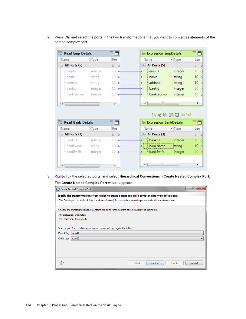
2. Press Ctrl and select the ports in the two transformations that you want to convert as elements of the nested complex port.
3. Right-click the selected ports, and select Hierarchical Conversions > Create Nested Complex Port.
The Create Nested Complex Port wizard appears.
114 Chapter 5: Processing Hierarchical Data on the Spark Engine
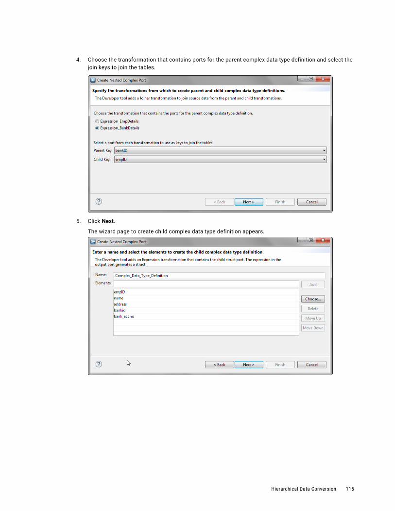
4. Choose the transformation that contains ports for the parent complex data type definition and select the join keys to join the tables.
5. Click Next.
The wizard page to create child complex data type definition appears.
Hierarchical Data Conversion 115
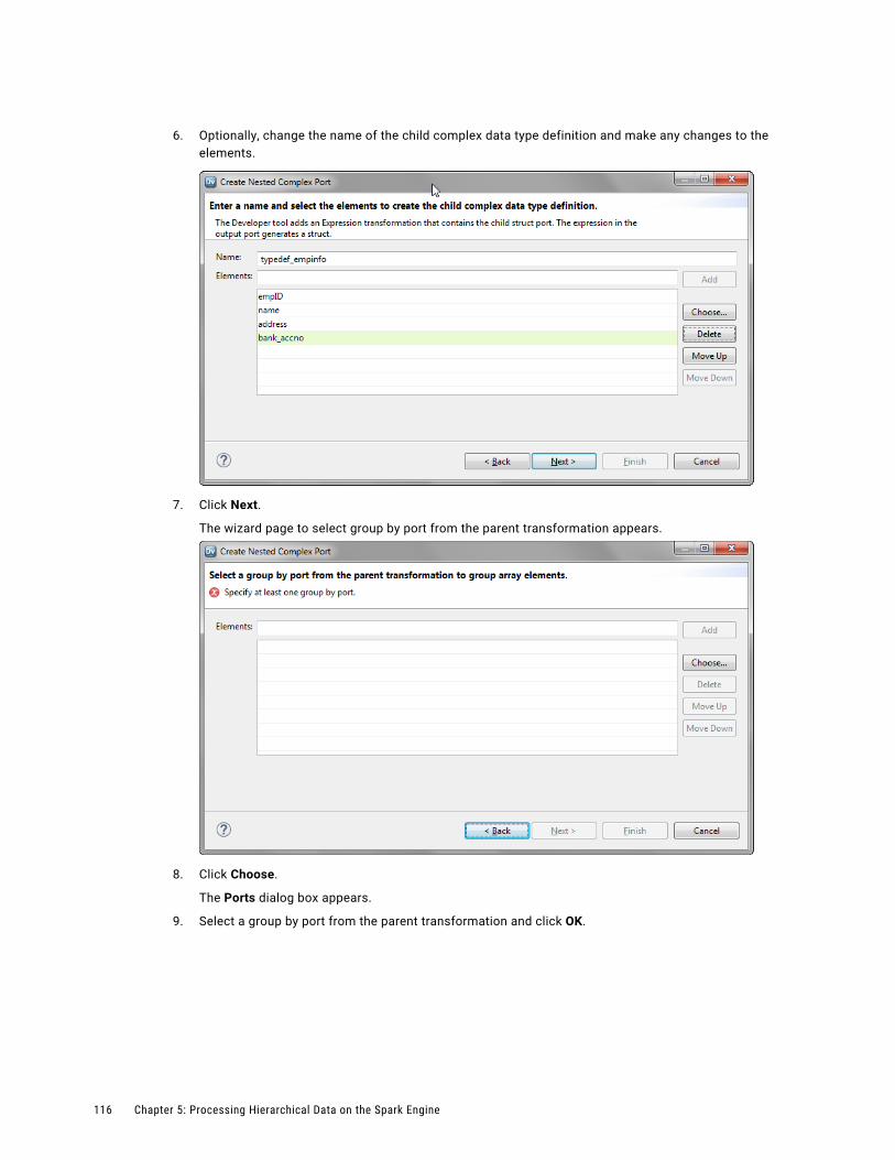
6. Optionally, change the name of the child complex data type definition and make any changes to the elements.
7. Click Next.
The wizard page to select group by port from the parent transformation appears.
8. Click Choose.
The Ports dialog box appears.
9. Select a group by port from the parent transformation and click OK.
116 Chapter 5: Processing Hierarchical Data on the Spark Engine
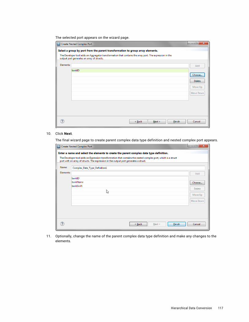
The selected port appears on the wizard page.
10. Click Next.
The final wizard page to create parent complex data type definition and nested complex port appears.
11. Optionally, change the name of the parent complex data type definition and make any changes to the elements.
Hierarchical Data Conversion 117
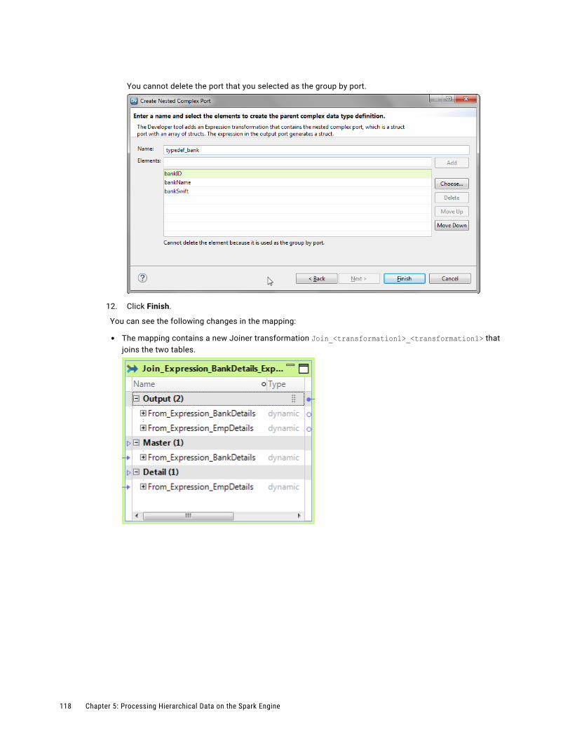
You cannot delete the port that you selected as the group by port.
12. Click Finish.
You can see the following changes in the mapping:
• The mapping contains a new Joiner transformation Join_<transformation1>_<transformation1> that joins the two tables.
118 Chapter 5: Processing Hierarchical Data on the Spark Engine

• The mapping contains a new Expression transformation Create_ChildStruct with a struct output port and a dynamic port with ports from the upstream transformation.
• The type definition library contains the new child complex data type definition. The struct output port references the child complex data type definition.
The output port contains an expression with the STRUCT_AS function:
STRUCT_AS(:Type.Type_Definition_Library.<child_typedef>,<comma_delimited_child_elements>)
• The mapping contains a new Aggregator transformation Agg_ArrayOfStruct with the group by port to group the child structs into an array.
Hierarchical Data Conversion 119
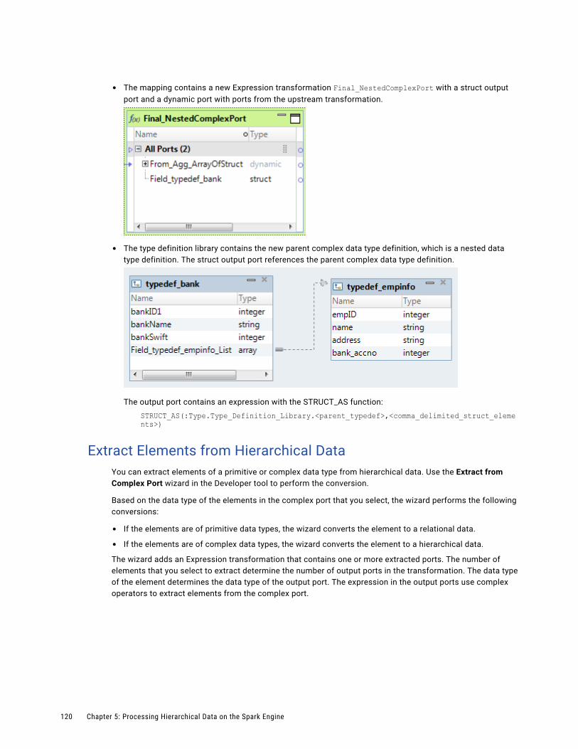
• The mapping contains a new Expression transformation Final_NestedComplexPort with a struct output port and a dynamic port with ports from the upstream transformation.
• The type definition library contains the new parent complex data type definition, which is a nested data type definition. The struct output port references the parent complex data type definition.
The output port contains an expression with the STRUCT_AS function:
STRUCT_AS(:Type.Type_Definition_Library.<parent_typedef>,<comma_delimited_struct_elements>)
Extract Elements from Hierarchical DataYou can extract elements of a primitive or complex data type from hierarchical data. Use the Extract from Complex Port wizard in the Developer tool to perform the conversion.
Based on the data type of the elements in the complex port that you select, the wizard performs the following conversions:
• If the elements are of primitive data types, the wizard converts the element to a relational data.
• If the elements are of complex data types, the wizard converts the element to a hierarchical data.
The wizard adds an Expression transformation that contains one or more extracted ports. The number of elements that you select to extract determine the number of output ports in the transformation. The data type of the element determines the data type of the output port. The expression in the output ports use complex operators to extract elements from the complex port.
120 Chapter 5: Processing Hierarchical Data on the Spark Engine
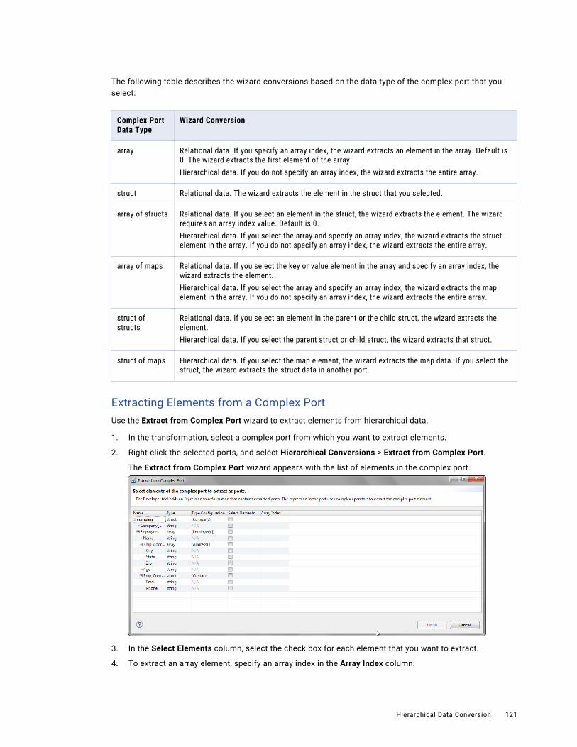
The following table describes the wizard conversions based on the data type of the complex port that you select:
Complex Port Data Type
Wizard Conversion
array Relational data. If you specify an array index, the wizard extracts an element in the array. Default is 0. The wizard extracts the first element of the array.Hierarchical data. If you do not specify an array index, the wizard extracts the entire array.
struct Relational data. The wizard extracts the element in the struct that you selected.
array of structs Relational data. If you select an element in the struct, the wizard extracts the element. The wizard requires an array index value. Default is 0.Hierarchical data. If you select the array and specify an array index, the wizard extracts the struct element in the array. If you do not specify an array index, the wizard extracts the entire array.
array of maps Relational data. If you select the key or value element in the array and specify an array index, the wizard extracts the element.Hierarchical data. If you select the array and specify an array index, the wizard extracts the map element in the array. If you do not specify an array index, the wizard extracts the entire array.
struct of structs
Relational data. If you select an element in the parent or the child struct, the wizard extracts the element.Hierarchical data. If you select the parent struct or child struct, the wizard extracts that struct.
struct of maps Hierarchical data. If you select the map element, the wizard extracts the map data. If you select the struct, the wizard extracts the struct data in another port.
Extracting Elements from a Complex PortUse the Extract from Complex Port wizard to extract elements from hierarchical data.
1. In the transformation, select a complex port from which you want to extract elements.
2. Right-click the selected ports, and select Hierarchical Conversions > Extract from Complex Port.
The Extract from Complex Port wizard appears with the list of elements in the complex port.
3. In the Select Elements column, select the check box for each element that you want to extract.
4. To extract an array element, specify an array index in the Array Index column.
Hierarchical Data Conversion 121
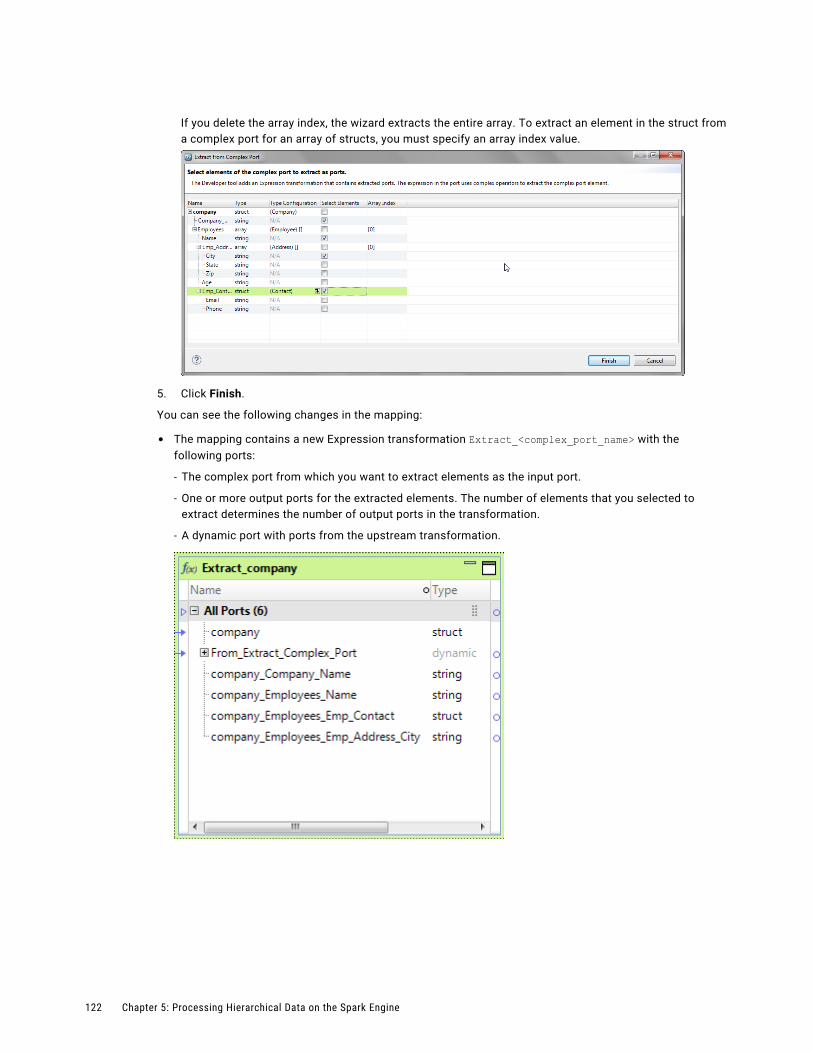
If you delete the array index, the wizard extracts the entire array. To extract an element in the struct from a complex port for an array of structs, you must specify an array index value.
5. Click Finish.
You can see the following changes in the mapping:
• The mapping contains a new Expression transformation Extract_<complex_port_name> with the following ports:
- The complex port from which you want to extract elements as the input port.
- One or more output ports for the extracted elements. The number of elements that you selected to extract determines the number of output ports in the transformation.
- A dynamic port with ports from the upstream transformation.
122 Chapter 5: Processing Hierarchical Data on the Spark Engine

• The output ports contain expressions that use complex operators to extract elements.The following image shows the expressions for the output ports in the Expression column on the Ports tab:
Flatten Hierarchical DataYou can flatten elements of hierarchical data into relational data. Use the Flatten Complex Port wizard in the Developer tool to perform the conversion.
The wizard converts hierarchical data to relational data. When you have hierarchical data with nested data type, you can select specific elements or all elements of complex data type to flatten.
Based on the data type of the complex port, the wizard performs the following tasks:
struct
• Adds an Expression transformation with flattened output ports. The expression for the output ports uses the dot operator to extract elements in the struct.
• Adds a final Expression transformation that contains a dynamic port with all ports from the upstream transformation including the flattened struct ports.
array
Adds a Normalizer transformation with flattened output ports. The wizard flattens the array field in the Normalizer view.
Adds a final Expression transformation that contains a dynamic port with all ports from the upstream transformation including the flattened array ports.
nested data type
Adds one or more Expression and Normalizer transformations with flattened output ports. If you select a child element of a nested complex port, the wizard flattens both the parent and child elements.
Adds a final Expression transformation that contains a dynamic port with all ports from the upstream transformation including the flattened ports.
Flattening a Complex PortUse the Flatten Complex Port wizard to convert hierarchical data to relational data.
1. In the transformation, select a complex port that you want to flatten.
2. Right-click the selected ports, and select Hierarchical Conversions > Flatten Complex Port.
Hierarchical Data Conversion 123

The Flatten Complex Port wizard appears with the list of elements in the complex port.
3. In the Select Elements column, select the check box for each element of a struct or an array data type that you want to extract.
If you select a child element of a nested complex port, the wizard automatically selects the parent element to flatten.
4. Optionally, click Flatten All to flatten all elements of struct or data type in the complex port.
The wizard selects all elements of struct or data type in the complex port to flatten.
5. Click Finish.
You can see the following changes in the mapping:
• For each struct element that you selected to flatten, the mapping contains a new Expression transformation Extract_<element_of_struct_type> with the following ports:
- The complex port from which you want to extract elements.
- One or more output ports for the extracted elements.The output ports contain expressions that use complex operators to extract elements.
- A dynamic port with ports from the upstream transformation
• For each array element that you selected to flatten, the mapping contains a new Normalizer transformation Flatten_<element_of_array_type> with an input group and an output group. The output group contains the flattened normalized fields for the array element.
124 Chapter 5: Processing Hierarchical Data on the Spark Engine
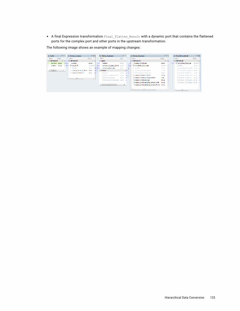
• A final Expression transformation Final_Flatten_Result with a dynamic port that contains the flattened ports for the complex port and other ports in the upstream transformation.
The following image shows an example of mapping changes:
Hierarchical Data Conversion 125
C h a p t e r 6
Stateful Computing on the Spark Engine
This chapter includes the following topics:
• Stateful Computing on the Spark Engine Overview, 126
• Windowing Configuration, 127
• Window Functions, 130
• Windowing Examples, 135
Stateful Computing on the Spark Engine OverviewYou can use window functions in Expression transformations to perform stateful computations on the Spark engine.
A stateful computation is a function that takes some state and returns a value along with a new state.
You can use a window function to perform stateful computations. A window function takes a small subset of a larger data set for processing and analysis.
Window functions operate on a group of rows and calculate a return value for every input row. This characteristic of window functions makes it easy to express data processing tasks that are difficult to express concisely without window functions.
Use window functions to perform the following tasks:
• Retrieve data from upstream or downstream rows.
• Calculate a cumulative sum based on a group of rows.
• Calculate a cumulative average based on a group of rows.
Before you define a window function in an Expression transformation, you must describe the window by configuring the windowing properties. Windowing properties include a frame specification, partition keys, and order keys. The frame specification states which rows are included in the overall calculation for the current row. The partition keys determine which rows are in the same partition. The order keys determine how rows in a partition are ordered.
After you configure windowing properties, you define a window function in the Expression transformation. Spark supports the window functions LEAD and LAG. You can also use aggregate functions as window functions in an Expression transformation.
126
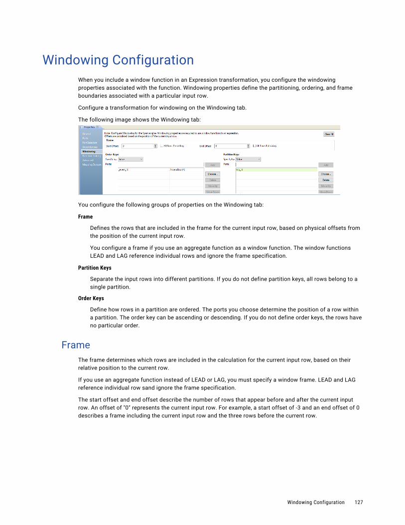
Windowing ConfigurationWhen you include a window function in an Expression transformation, you configure the windowing properties associated with the function. Windowing properties define the partitioning, ordering, and frame boundaries associated with a particular input row.
Configure a transformation for windowing on the Windowing tab.
The following image shows the Windowing tab:
You configure the following groups of properties on the Windowing tab:
Frame
Defines the rows that are included in the frame for the current input row, based on physical offsets from the position of the current input row.
You configure a frame if you use an aggregate function as a window function. The window functions LEAD and LAG reference individual rows and ignore the frame specification.
Partition Keys
Separate the input rows into different partitions. If you do not define partition keys, all rows belong to a single partition.
Order Keys
Define how rows in a partition are ordered. The ports you choose determine the position of a row within a partition. The order key can be ascending or descending. If you do not define order keys, the rows have no particular order.
FrameThe frame determines which rows are included in the calculation for the current input row, based on their relative position to the current row.
If you use an aggregate function instead of LEAD or LAG, you must specify a window frame. LEAD and LAG reference individual row sand ignore the frame specification.
The start offset and end offset describe the number of rows that appear before and after the current input row. An offset of "0" represents the current input row. For example, a start offset of -3 and an end offset of 0 describes a frame including the current input row and the three rows before the current row.
Windowing Configuration 127

The following image shows a frame with a start offset of -1 and an end offset of 1:
For every input row, the function performs an aggregate operation on the rows inside the frame. If you configure an aggregate expression like SUM with the preceding frame, the expression calculates the sum of the values within the frame and returns a value of 6000 for the input row.
You can also specify a frame that does not include the current input row. For example, a start offset of 10 and an end offset of 15 describes a frame that includes six total rows, from the tenth to the fifteenth row after the current row.
Note: The start offset must be less than or equal to the end offset.
Offsets of All Rows Preceding and All Rows Following represent the first row of the partition and the last row of the partition. For example, if the start offset is All Rows Preceding and the end offset is -1, the frame includes one row before the current row and all rows before that.
The following figure illustrates a frame with a start offset of 0 and an end offset of All Rows Following:
Partition and Order KeysConfigure partition and order keys to form groups of rows and define the order or sequence of rows within each partition.
Use the following keys to specify how to group and order the rows in a window:
Partition keys
Configure partition keys to define partition boundaries, rather than performing the calculation across all inputs. The window function operates across the rows that fall into the same partition as the current row.
128 Chapter 6: Stateful Computing on the Spark Engine
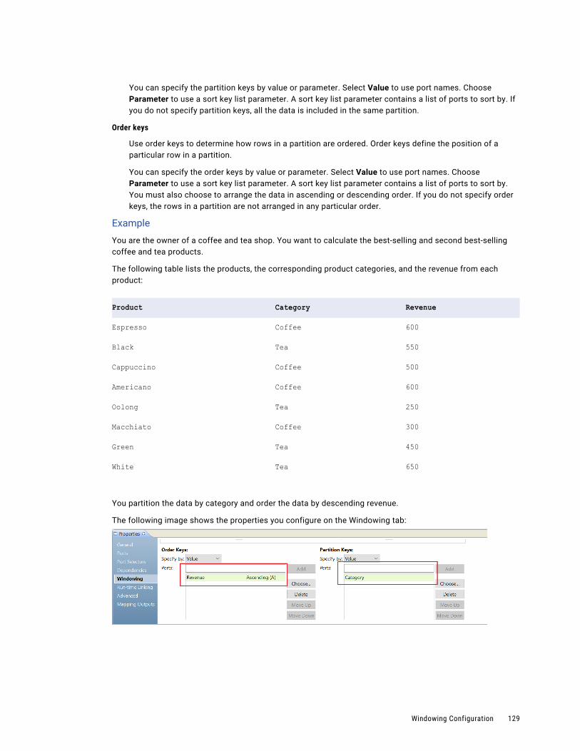
You can specify the partition keys by value or parameter. Select Value to use port names. Choose Parameter to use a sort key list parameter. A sort key list parameter contains a list of ports to sort by. If you do not specify partition keys, all the data is included in the same partition.
Order keys
Use order keys to determine how rows in a partition are ordered. Order keys define the position of a particular row in a partition.
You can specify the order keys by value or parameter. Select Value to use port names. Choose Parameter to use a sort key list parameter. A sort key list parameter contains a list of ports to sort by. You must also choose to arrange the data in ascending or descending order. If you do not specify order keys, the rows in a partition are not arranged in any particular order.
Example
You are the owner of a coffee and tea shop. You want to calculate the best-selling and second best-selling coffee and tea products.
The following table lists the products, the corresponding product categories, and the revenue from each product:
Product Category Revenue
Espresso Coffee 600
Black Tea 550
Cappuccino Coffee 500
Americano Coffee 600
Oolong Tea 250
Macchiato Coffee 300
Green Tea 450
White Tea 650
You partition the data by category and order the data by descending revenue.
The following image shows the properties you configure on the Windowing tab:
Windowing Configuration 129
The following table shows the data grouped into two partitions according to category. Within each partition, the revenue is organized in descending order:
Product Category Revenue
Espresso Coffee 600
Americano Coffee 600
Cappuccino Coffee 500
Macchiato Coffee 300
White Tea 650
Black Tea 550
Green Tea 450
Oolong Tea 250
Based on the partitioning and ordering specifications, you determine that the two best-selling coffees are espresso and Americano, and the two best-selling teas are white and black.
Rules and Guidelines for Windowing ConfigurationCertain guidelines apply when you configure a transformation for windowing.
Consider the following rules and guidelines when you define windowing properties for a window function:
• When you configure a frame, the start offset must be less than or equal to the end offset. Otherwise, the frame is not valid.
• Configure a frame specification if you use an aggregate function as a window function. LEAD and LAG operate based on the offset value and ignore the frame specification.
• You cannot use complex ports as partition or order keys.
• You cannot preview the data in a transformation configured for windowing.
• Assign unique port names to partition and order keys to avoid run-time errors.
• The partition and order keys cannot use both a dynamic port and one or more generated ports of the same dynamic port. You must select either the dynamic port or the generated ports.
Window FunctionsWindow functions calculate a return value for every input row of a table, based on a group of rows.
A window function performs a calculation across a set of table rows that are related to the current row. You can also perform this type of calculation with an aggregate function. But unlike regular aggregate functions, a window function does not group rows into a single output row. The rows retain unique identities.
You can define the LEAD and LAG analytic window functions in an Expression transformation. LEAD and LAG give access to multiple rows within a table, without the need for a self-join.
130 Chapter 6: Stateful Computing on the Spark Engine

LEADThe LEAD function returns data from future rows.
LEAD uses the following syntax:
LEAD ( Column name, Offset, Default )LEAD returns the value at an offset number of rows after the current row. Use the LEAD function to compare values in the current row with values in a following row. Use the following arguments with the LEAD function:
• Column name. The column name whose value from the subsequent row is to be returned.
• Offset. The number of rows following the current row from which the data is to be retrieved. For example, an offset of "1" accesses the next immediate row, and an offset of "3" accesses the third row after the current row.
• Default. The default value to be returned if the offset is outside the scope of the partition. If you do not specify a default, the default is NULL.
For more information about the LEAD function, see the Informatica Transformation Language Reference.
LAGThe LAG function returns data from preceding rows.
LAG uses the following syntax:
LAG ( Column name, Offset, Default )LAG returns the value at an offset number of rows before the current row. Use the LAG function to compare values in the current row with values in a previous row. Use the following arguments with the LAG function:
• Column name. The column name whose value from the prior row is to be returned.
• Offset. The number of rows preceding the current row from which the data is to be retrieved. For example, an offset of "1" accesses the previous row, and an offset of "3" accesses the row that is three rows before the current row.
• Default. The default value to be returned if the offset is outside the scope of the partition. If you do not specify a default, the default is NULL.
For more information about the LAG function, see the Informatica Transformation Language Reference.
Aggregate Functions as Window FunctionsIn addition to LEAD and LAG, you can also use aggregate functions as window functions. When you use aggregate functions like SUM and AVG as window functions, you can perform running calculations that are similar to the stateful functions MOVINGSUM, MOVINGAVG, and CUME. Window functions are more flexible than stateful functions because you can set a specific end offset.
To use an aggregate function as a window function, you must define a frame in the windowing properties. You define a frame to limit the scope of the calculation. The aggregate function performs a calculation across the frame and produces a single value for each row.
Example
You are a lumber salesperson who sold different quantities of wood over the past two years. You want to calculate a running total of sales quantities.
Window Functions 131
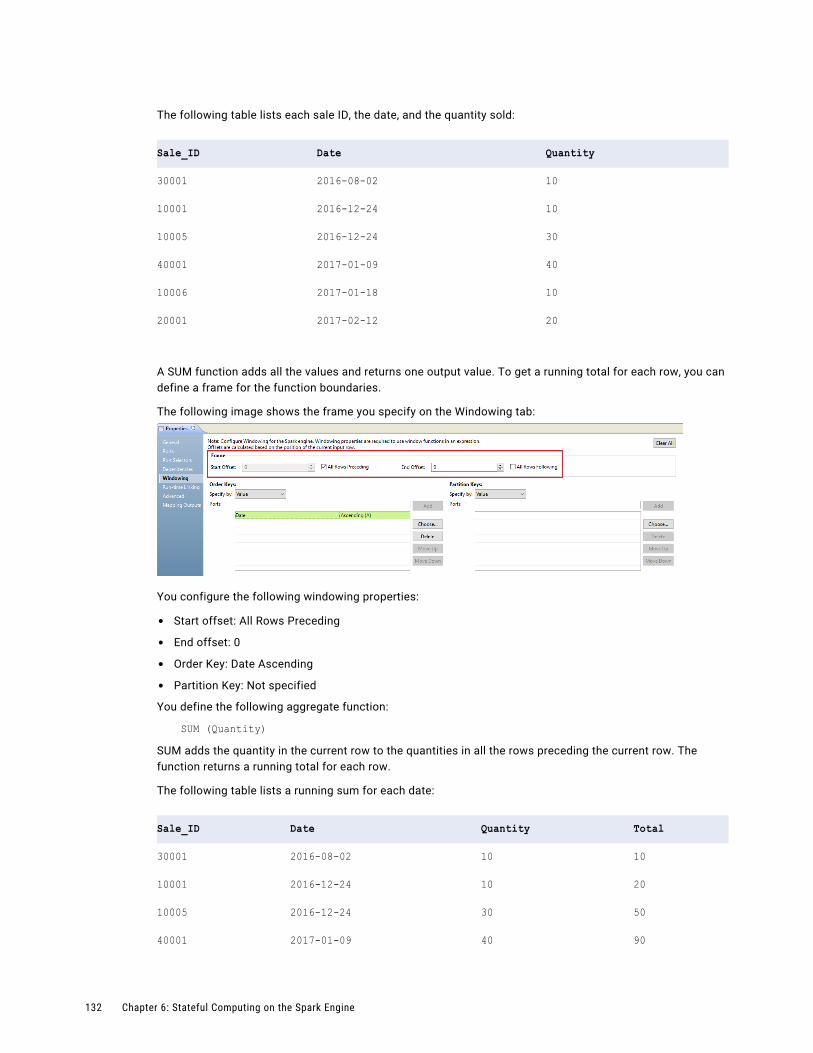
The following table lists each sale ID, the date, and the quantity sold:
Sale_ID Date Quantity
30001 2016-08-02 10
10001 2016-12-24 10
10005 2016-12-24 30
40001 2017-01-09 40
10006 2017-01-18 10
20001 2017-02-12 20
A SUM function adds all the values and returns one output value. To get a running total for each row, you can define a frame for the function boundaries.
The following image shows the frame you specify on the Windowing tab:
You configure the following windowing properties:
• Start offset: All Rows Preceding
• End offset: 0
• Order Key: Date Ascending
• Partition Key: Not specified
You define the following aggregate function:
SUM (Quantity)SUM adds the quantity in the current row to the quantities in all the rows preceding the current row. The function returns a running total for each row.
The following table lists a running sum for each date:
Sale_ID Date Quantity Total
30001 2016-08-02 10 10
10001 2016-12-24 10 20
10005 2016-12-24 30 50
40001 2017-01-09 40 90
132 Chapter 6: Stateful Computing on the Spark Engine
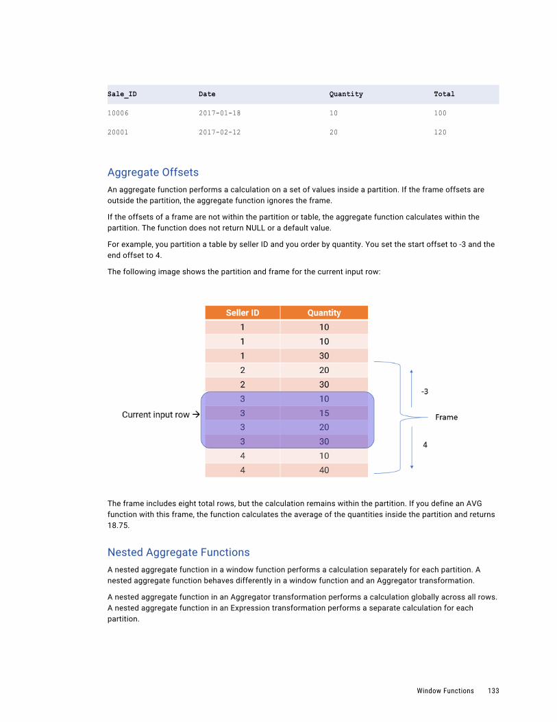
Sale_ID Date Quantity Total
10006 2017-01-18 10 100
20001 2017-02-12 20 120
Aggregate OffsetsAn aggregate function performs a calculation on a set of values inside a partition. If the frame offsets are outside the partition, the aggregate function ignores the frame.
If the offsets of a frame are not within the partition or table, the aggregate function calculates within the partition. The function does not return NULL or a default value.
For example, you partition a table by seller ID and you order by quantity. You set the start offset to -3 and the end offset to 4.
The following image shows the partition and frame for the current input row:
The frame includes eight total rows, but the calculation remains within the partition. If you define an AVG function with this frame, the function calculates the average of the quantities inside the partition and returns 18.75.
Nested Aggregate FunctionsA nested aggregate function in a window function performs a calculation separately for each partition. A nested aggregate function behaves differently in a window function and an Aggregator transformation.
A nested aggregate function in an Aggregator transformation performs a calculation globally across all rows. A nested aggregate function in an Expression transformation performs a separate calculation for each partition.
Window Functions 133
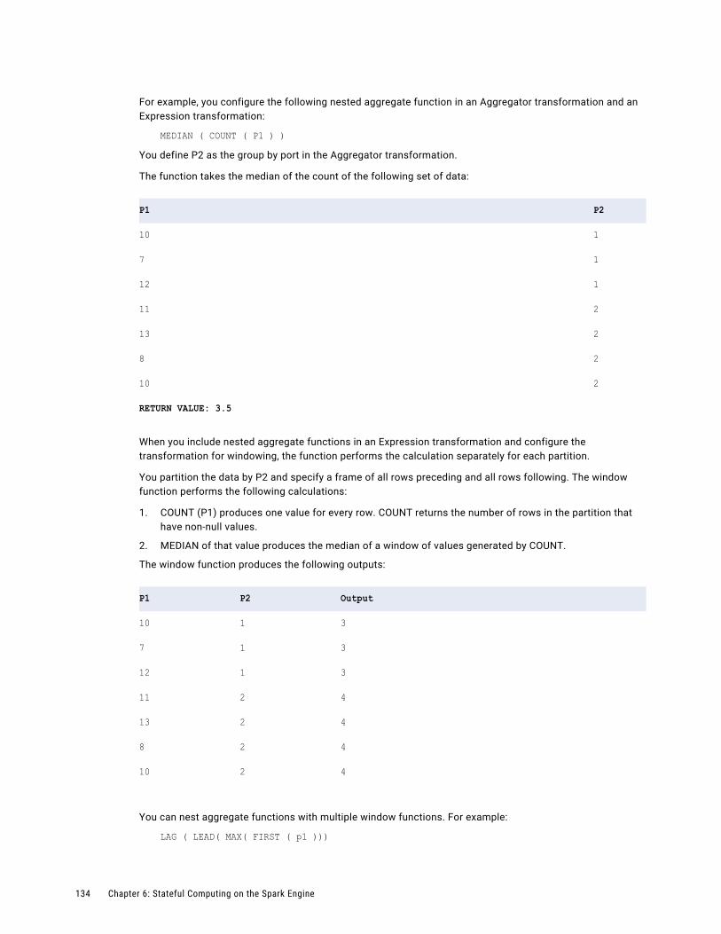
For example, you configure the following nested aggregate function in an Aggregator transformation and an Expression transformation:
MEDIAN ( COUNT ( P1 ) ) You define P2 as the group by port in the Aggregator transformation.
The function takes the median of the count of the following set of data:
P1 P2
10 1
7 1
12 1
11 2
13 2
8 2
10 2
RETURN VALUE: 3.5
When you include nested aggregate functions in an Expression transformation and configure the transformation for windowing, the function performs the calculation separately for each partition.
You partition the data by P2 and specify a frame of all rows preceding and all rows following. The window function performs the following calculations:
1. COUNT (P1) produces one value for every row. COUNT returns the number of rows in the partition that have non-null values.
2. MEDIAN of that value produces the median of a window of values generated by COUNT.
The window function produces the following outputs:
P1 P2 Output
10 1 3
7 1 3
12 1 3
11 2 4
13 2 4
8 2 4
10 2 4
You can nest aggregate functions with multiple window functions. For example:
LAG ( LEAD( MAX( FIRST ( p1 )))
134 Chapter 6: Stateful Computing on the Spark Engine
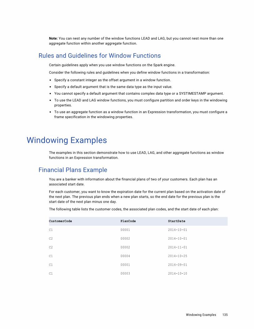
Note: You can nest any number of the window functions LEAD and LAG, but you cannot nest more than one aggregate function within another aggregate function.
Rules and Guidelines for Window FunctionsCertain guidelines apply when you use window functions on the Spark engine.
Consider the following rules and guidelines when you define window functions in a transformation:
• Specify a constant integer as the offset argument in a window function.
• Specify a default argument that is the same data type as the input value.
• You cannot specify a default argument that contains complex data type or a SYSTIMESTAMP argument.
• To use the LEAD and LAG window functions, you must configure partition and order keys in the windowing properties.
• To use an aggregate function as a window function in an Expression transformation, you must configure a frame specification in the windowing properties.
Windowing ExamplesThe examples in this section demonstrate how to use LEAD, LAG, and other aggregate functions as window functions in an Expression transformation.
Financial Plans ExampleYou are a banker with information about the financial plans of two of your customers. Each plan has an associated start date.
For each customer, you want to know the expiration date for the current plan based on the activation date of the next plan. The previous plan ends when a new plan starts, so the end date for the previous plan is the start date of the next plan minus one day.
The following table lists the customer codes, the associated plan codes, and the start date of each plan:
CustomerCode PlanCode StartDate
C1 00001 2014-10-01
C2 00002 2014-10-01
C2 00002 2014-11-01
C1 00004 2014-10-25
C1 00001 2014-09-01
C1 00003 2014-10-10
Windowing Examples 135
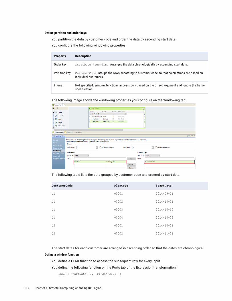
Define partition and order keys
You partition the data by customer code and order the data by ascending start date.
You configure the following windowing properties:
Property Description
Order key StartDate Ascending. Arranges the data chronologically by ascending start date.
Partition key CustomerCode. Groups the rows according to customer code so that calculations are based on individual customers.
Frame Not specified. Window functions access rows based on the offset argument and ignore the frame specification.
The following image shows the windowing properties you configure on the Windowing tab:
The following table lists the data grouped by customer code and ordered by start date:
CustomerCode PlanCode StartDate
C1 00001 2014-09-01
C1 00002 2014-10-01
C1 00003 2014-10-10
C1 00004 2014-10-25
C2 00001 2014-10-01
C2 00002 2014-11-01
The start dates for each customer are arranged in ascending order so that the dates are chronological.
Define a window function
You define a LEAD function to access the subsequent row for every input.
You define the following function on the Ports tab of the Expression transformation:
LEAD ( StartDate, 1, '01-Jan-2100' )
136 Chapter 6: Stateful Computing on the Spark Engine
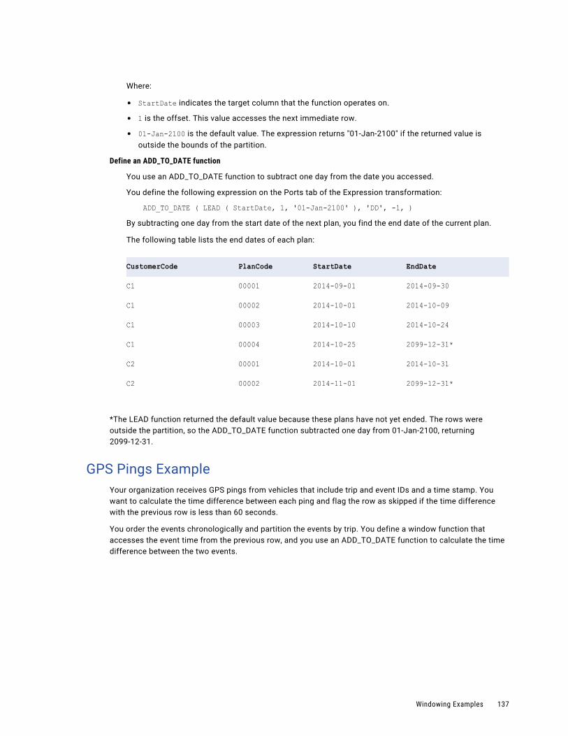
Where:
• StartDate indicates the target column that the function operates on.
• 1 is the offset. This value accesses the next immediate row.
• 01-Jan-2100 is the default value. The expression returns "01-Jan-2100" if the returned value is outside the bounds of the partition.
Define an ADD_TO_DATE function
You use an ADD_TO_DATE function to subtract one day from the date you accessed.
You define the following expression on the Ports tab of the Expression transformation:
ADD_TO_DATE ( LEAD ( StartDate, 1, '01-Jan-2100' ), 'DD', -1, )By subtracting one day from the start date of the next plan, you find the end date of the current plan.
The following table lists the end dates of each plan:
CustomerCode PlanCode StartDate EndDate
C1 00001 2014-09-01 2014-09-30
C1 00002 2014-10-01 2014-10-09
C1 00003 2014-10-10 2014-10-24
C1 00004 2014-10-25 2099-12-31*
C2 00001 2014-10-01 2014-10-31
C2 00002 2014-11-01 2099-12-31*
*The LEAD function returned the default value because these plans have not yet ended. The rows were outside the partition, so the ADD_TO_DATE function subtracted one day from 01-Jan-2100, returning 2099-12-31.
GPS Pings ExampleYour organization receives GPS pings from vehicles that include trip and event IDs and a time stamp. You want to calculate the time difference between each ping and flag the row as skipped if the time difference with the previous row is less than 60 seconds.
You order the events chronologically and partition the events by trip. You define a window function that accesses the event time from the previous row, and you use an ADD_TO_DATE function to calculate the time difference between the two events.
Windowing Examples 137
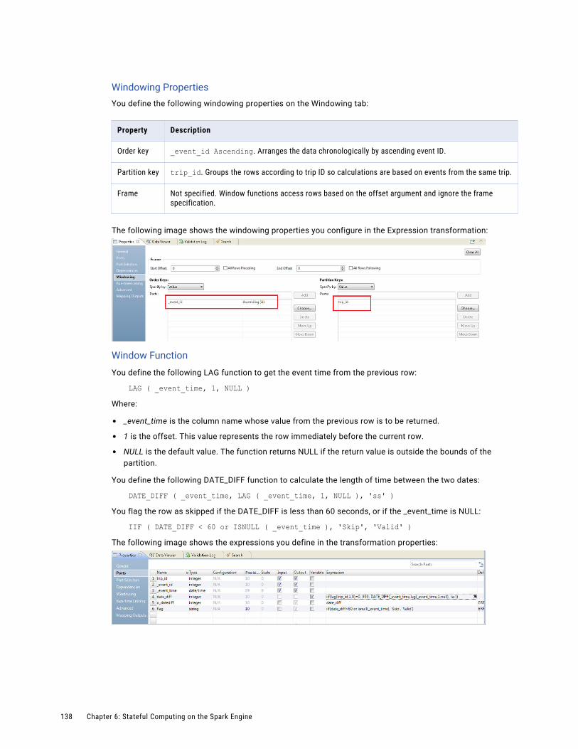
Windowing PropertiesYou define the following windowing properties on the Windowing tab:
Property Description
Order key _event_id Ascending. Arranges the data chronologically by ascending event ID.
Partition key trip_id. Groups the rows according to trip ID so calculations are based on events from the same trip.
Frame Not specified. Window functions access rows based on the offset argument and ignore the frame specification.
The following image shows the windowing properties you configure in the Expression transformation:
Window Function
You define the following LAG function to get the event time from the previous row:
LAG ( _event_time, 1, NULL )Where:
• _event_time is the column name whose value from the previous row is to be returned.
• 1 is the offset. This value represents the row immediately before the current row.
• NULL is the default value. The function returns NULL if the return value is outside the bounds of the partition.
You define the following DATE_DIFF function to calculate the length of time between the two dates:
DATE_DIFF ( _event_time, LAG ( _event_time, 1, NULL ), 'ss' )You flag the row as skipped if the DATE_DIFF is less than 60 seconds, or if the _event_time is NULL:
IIF ( DATE_DIFF < 60 or ISNULL ( _event_time ), 'Skip', 'Valid' )The following image shows the expressions you define in the transformation properties:
138 Chapter 6: Stateful Computing on the Spark Engine
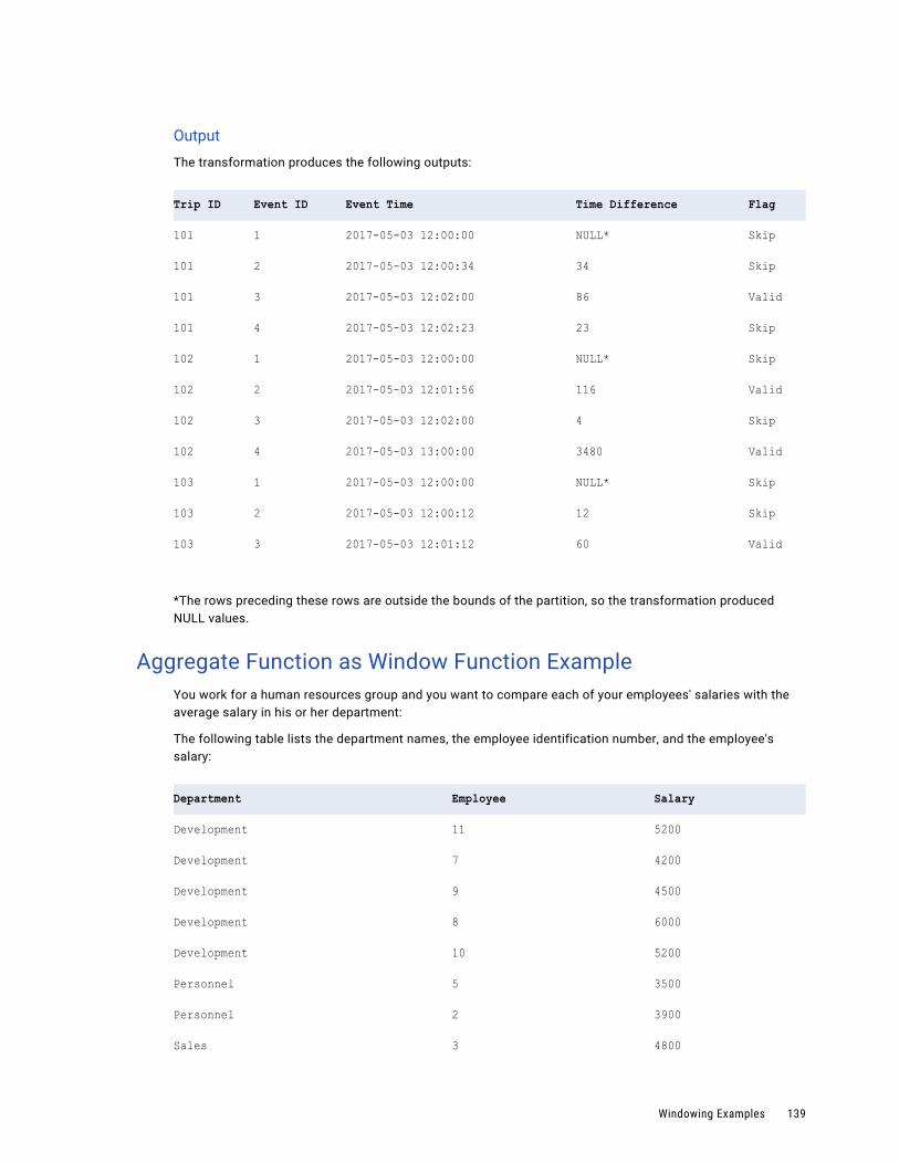
Output
The transformation produces the following outputs:
Trip ID Event ID Event Time Time Difference Flag
101 1 2017-05-03 12:00:00 NULL* Skip
101 2 2017-05-03 12:00:34 34 Skip
101 3 2017-05-03 12:02:00 86 Valid
101 4 2017-05-03 12:02:23 23 Skip
102 1 2017-05-03 12:00:00 NULL* Skip
102 2 2017-05-03 12:01:56 116 Valid
102 3 2017-05-03 12:02:00 4 Skip
102 4 2017-05-03 13:00:00 3480 Valid
103 1 2017-05-03 12:00:00 NULL* Skip
103 2 2017-05-03 12:00:12 12 Skip
103 3 2017-05-03 12:01:12 60 Valid
*The rows preceding these rows are outside the bounds of the partition, so the transformation produced NULL values.
Aggregate Function as Window Function ExampleYou work for a human resources group and you want to compare each of your employees' salaries with the average salary in his or her department:
The following table lists the department names, the employee identification number, and the employee's salary:
Department Employee Salary
Development 11 5200
Development 7 4200
Development 9 4500
Development 8 6000
Development 10 5200
Personnel 5 3500
Personnel 2 3900
Sales 3 4800
Windowing Examples 139
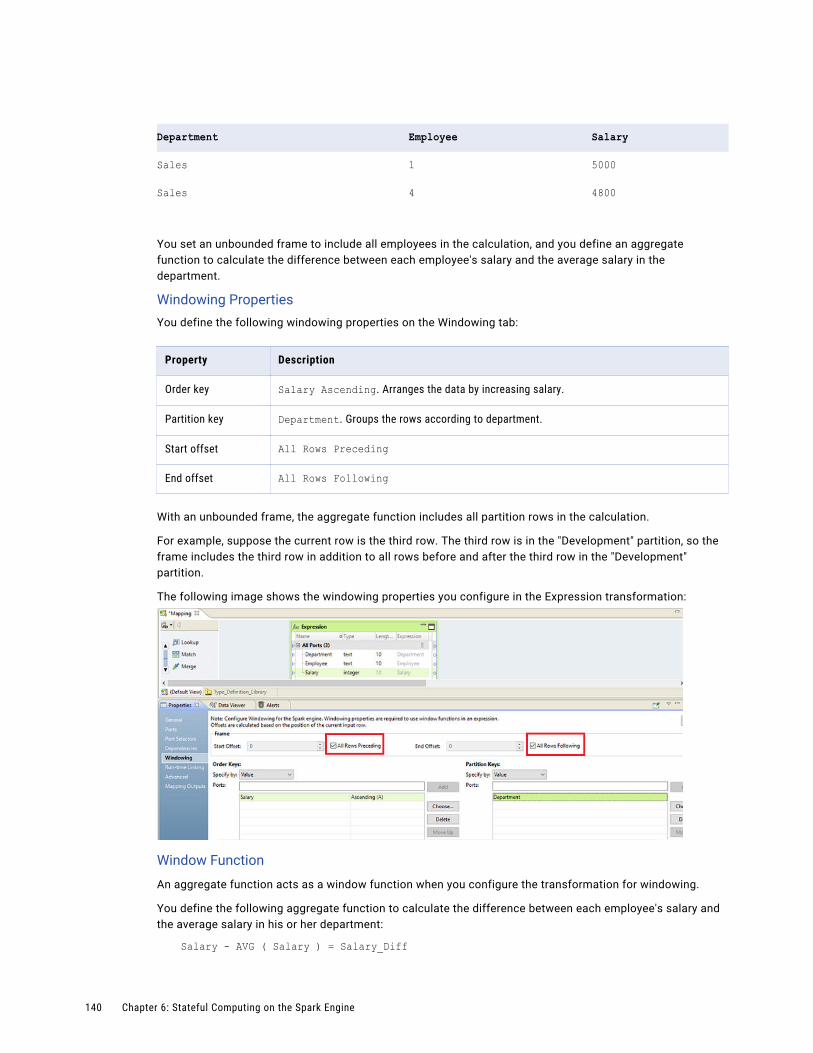
Department Employee Salary
Sales 1 5000
Sales 4 4800
You set an unbounded frame to include all employees in the calculation, and you define an aggregate function to calculate the difference between each employee's salary and the average salary in the department.
Windowing PropertiesYou define the following windowing properties on the Windowing tab:
Property Description
Order key Salary Ascending. Arranges the data by increasing salary.
Partition key Department. Groups the rows according to department.
Start offset All Rows Preceding
End offset All Rows Following
With an unbounded frame, the aggregate function includes all partition rows in the calculation.
For example, suppose the current row is the third row. The third row is in the "Development" partition, so the frame includes the third row in addition to all rows before and after the third row in the "Development" partition.
The following image shows the windowing properties you configure in the Expression transformation:
Window Function
An aggregate function acts as a window function when you configure the transformation for windowing.
You define the following aggregate function to calculate the difference between each employee's salary and the average salary in his or her department:
Salary - AVG ( Salary ) = Salary_Diff
140 Chapter 6: Stateful Computing on the Spark Engine
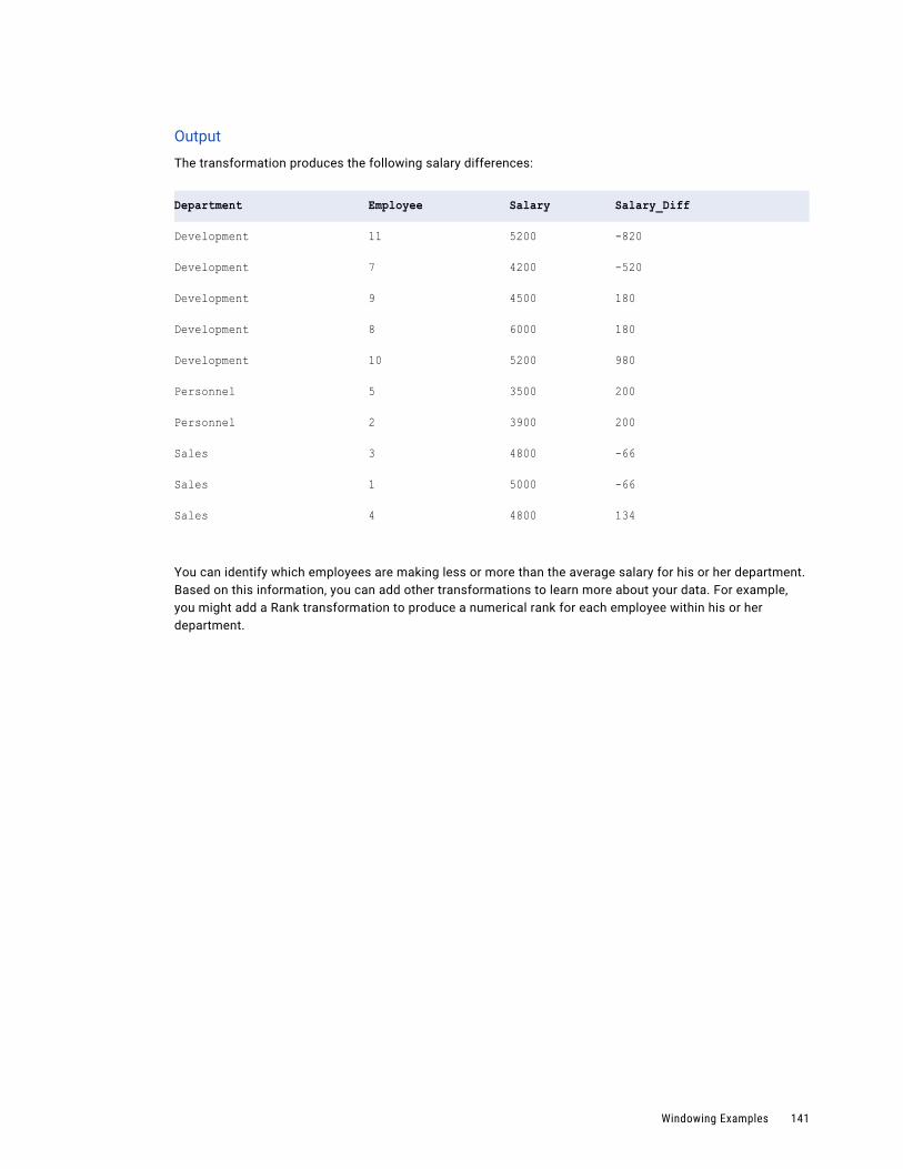
Output
The transformation produces the following salary differences:
Department Employee Salary Salary_Diff
Development 11 5200 -820
Development 7 4200 -520
Development 9 4500 180
Development 8 6000 180
Development 10 5200 980
Personnel 5 3500 200
Personnel 2 3900 200
Sales 3 4800 -66
Sales 1 5000 -66
Sales 4 4800 134
You can identify which employees are making less or more than the average salary for his or her department. Based on this information, you can add other transformations to learn more about your data. For example, you might add a Rank transformation to produce a numerical rank for each employee within his or her department.
Windowing Examples 141
C h a p t e r 7
Monitoring Mappings in the Hadoop Environment
This chapter includes the following topics:
• Monitoring Mappings in the Hadoop Environment Overview, 142
• Hadoop Environment Logs, 142
• Blaze Engine Monitoring, 146
• Spark Engine Monitoring, 154
• Hive Engine Monitoring, 157
Monitoring Mappings in the Hadoop Environment Overview
On the Monitor tab of the Administrator tool, you can view statistics and log events for mappings run in the Hadoop environment.
The Monitor tab displays current and historical information about mappings run on Blaze, Spark, and Hive engines. Use the Summary Statistics view to view graphical summaries of object state and distribution across the Data Integration Services. You can also view graphs of the memory and CPU that the Data Integration Services used to run the objects.
The Data Integration Service also generates log events when you run a mapping in the Hadoop environment. You can view log events relating to different types of errors such as Hadoop connection failures, Hive query failures, Hive command failures, or other Hadoop job failures.
Hadoop Environment LogsThe Data Integration Service generates log events when you run a mapping in the Hadoop environment.
You can view logs for the Blaze engine, the Spark engine, or the Hive on MapReduce engine. You can view log events relating to different types of errors such as Hadoop connection failures, Hive query failures, Hive command failures, or other Hadoop job failures.
142
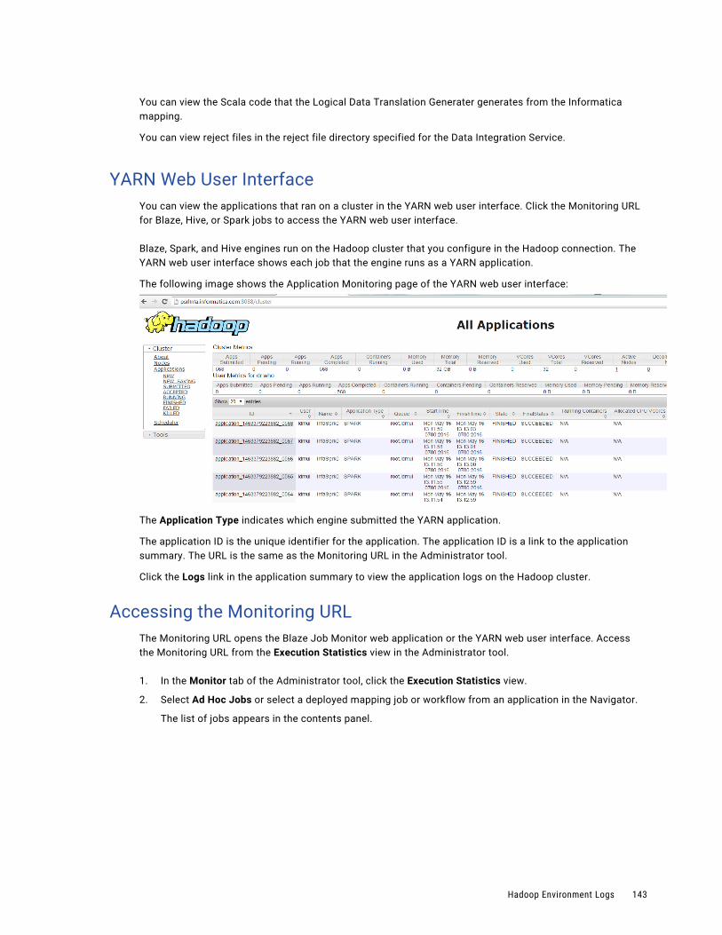
You can view the Scala code that the Logical Data Translation Generater generates from the Informatica mapping.
You can view reject files in the reject file directory specified for the Data Integration Service.
YARN Web User InterfaceYou can view the applications that ran on a cluster in the YARN web user interface. Click the Monitoring URL for Blaze, Hive, or Spark jobs to access the YARN web user interface.
Blaze, Spark, and Hive engines run on the Hadoop cluster that you configure in the Hadoop connection. The YARN web user interface shows each job that the engine runs as a YARN application.
The following image shows the Application Monitoring page of the YARN web user interface:
The Application Type indicates which engine submitted the YARN application.
The application ID is the unique identifier for the application. The application ID is a link to the application summary. The URL is the same as the Monitoring URL in the Administrator tool.
Click the Logs link in the application summary to view the application logs on the Hadoop cluster.
Accessing the Monitoring URLThe Monitoring URL opens the Blaze Job Monitor web application or the YARN web user interface. Access the Monitoring URL from the Execution Statistics view in the Administrator tool.
1. In the Monitor tab of the Administrator tool, click the Execution Statistics view.
2. Select Ad Hoc Jobs or select a deployed mapping job or workflow from an application in the Navigator.
The list of jobs appears in the contents panel.
Hadoop Environment Logs 143

3. Select a mapping job and expand the mapping to select a grid task for the mapping.
The Monitoring URL appears in the Properties view.
Viewing Hadoop Environment Logs in the Administrator ToolYou can view log events for a Blaze or Hive mapping from the Monitor tab of the Administrator tool.
1. In the Administrator tool, click the Monitor tab.
2. Select the Execution Statistics view.
3. In the Navigator, choose to open an ad hoc job, a deployed mapping job, or a workflow.
• To choose an ad hoc job, expand a Data Integration Service and click Ad Hoc Jobs.
• To choose a deployed mapping job, expand an application and click Deployed Mapping Jobs.
• To choose a workflow, expand an application and click Workflows.
The list of jobs appears in the contents panel.
4. Click Actions > View Logs for Selected Object to view the run-time logs for the mapping.
The log file shows the results of the Hive queries and Blaze engine queries run by the Data Integration Service. This includes the location of Hive session logs and Hive session history file.
144 Chapter 7: Monitoring Mappings in the Hadoop Environment

Monitoring a MappingYou can monitor a mapping that runs in the Hadoop environment.
1. In the Administrator tool, click the Monitor tab.
2. Select the Execution Statistics view.
3. In the Navigator, choose to open an ad hoc job, a deployed mapping job, or a workflow.
• To choose an ad hoc job, expand a Data Integration Service and click Ad Hoc Jobs.
• To choose a deployed mapping job, expand an application and click Deployed Mapping Jobs.
• To choose a workflow, expand an application and click Workflows.
The list of jobs appears in the contents panel.
4. Click a job to view its properties.
The contents panel shows the default Properties view for the job. For a Blaze engine mapping, the Blaze engine monitoring URL appears in the general properties in the details panel. The monitoring URL is a link to the YARN web user interface for Spark jobs.
5. Choose a view in the contents panel to view more information about the job:
• To view the execution plan for the mapping, select the Execution Plan view.
• To view the summary statistics for a job, click the Summary Statistics view.
• To view the detailed statistics for a job, click the Detailed Statistics view.
Hadoop Environment Logs 145
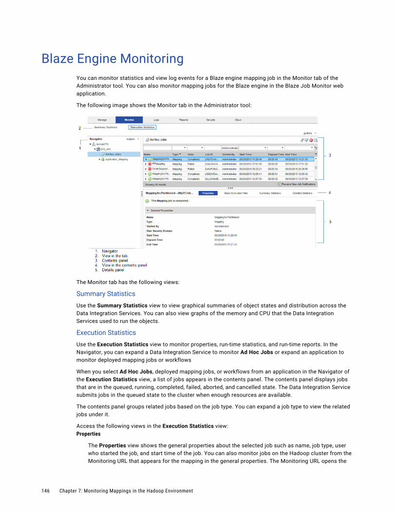
Blaze Engine MonitoringYou can monitor statistics and view log events for a Blaze engine mapping job in the Monitor tab of the Administrator tool. You can also monitor mapping jobs for the Blaze engine in the Blaze Job Monitor web application.
The following image shows the Monitor tab in the Administrator tool:
The Monitor tab has the following views:
Summary Statistics
Use the Summary Statistics view to view graphical summaries of object states and distribution across the Data Integration Services. You can also view graphs of the memory and CPU that the Data Integration Services used to run the objects.
Execution Statistics
Use the Execution Statistics view to monitor properties, run-time statistics, and run-time reports. In the Navigator, you can expand a Data Integration Service to monitor Ad Hoc Jobs or expand an application to monitor deployed mapping jobs or workflows
When you select Ad Hoc Jobs, deployed mapping jobs, or workflows from an application in the Navigator of the Execution Statistics view, a list of jobs appears in the contents panel. The contents panel displays jobs that are in the queued, running, completed, failed, aborted, and cancelled state. The Data Integration Service submits jobs in the queued state to the cluster when enough resources are available.
The contents panel groups related jobs based on the job type. You can expand a job type to view the related jobs under it.
Access the following views in the Execution Statistics view:Properties
The Properties view shows the general properties about the selected job such as name, job type, user who started the job, and start time of the job. You can also monitor jobs on the Hadoop cluster from the Monitoring URL that appears for the mapping in the general properties. The Monitoring URL opens the
146 Chapter 7: Monitoring Mappings in the Hadoop Environment
Blaze Job Monitor in a web page. The Blaze Job Monitor displays detailed monitoring statistics for a mapping such as the number of grid tasks, grid segments, or tasklets, and recovery attempts for each tasklet.
Blaze Execution Plan
The Blaze execution plan displays the Blaze engine script that the Data Integration Service generates based on the mapping logic. The execution plan includes the tasks that the script depends on. Each script has a unique identifier.
Summary Statistics
The Summary Statistics view appears in the details panel when you select a mapping job in the contents panel. The Summary Statistics view displays throughput and resource usage statistics for the job.
You can view the following throughput statistics for the job:
• Source. The name of the mapping source file.
• Target name. The name of the target file.
• Rows. The number of rows read for source and target. If the target is Hive, this is the only summary statistic available.
• Average Rows/Sec. Average number of rows read per second for source and target.
• Bytes. Number of bytes read for source and target.
• Average Bytes/Sec. Average number of bytes read per second for source and target.
• First Row Accessed. The date and time when the Data Integration Service started reading the first row in the source file.
• Dropped rows. Number of source rows that the Data Integration Service did not read.
Detailed Statistics
The Detailed Statistics view appears in the details panel when you select a mapping job in the contents panel. The Detailed Statistics view displays graphs of the throughput and resource usage statistics for the job run.
Blaze Job Monitoring ApplicationUse the Blaze Job Monitor application to monitor Blaze engine jobs on the Hadoop cluster.
You configure the host that starts the Blaze Job Monitor in the Hadoop connection properties. You might want to configure the Blaze Job Monitor address to avoid conflicts with other users on the same cluster, or if you have access to a limited number of nodes. If you do not configure the Blaze Job Monitor address, the Grid Manager starts the host on the first alphabetical cluster node with a default port of 9080.
The Blaze engine monitoring URL appears in the Monitor tab of the Administrator tool when you view a Blaze engine mapping job. When you click the URL, the Blaze engine monitoring application opens in a web page.
Note: You can also access the Blaze Job Monitor through the LDTM log. After the session load summary, the log displays a list of segments within the grid task. Each segment contains a link to the Blaze Job Monitor. Click on a link to see the execution details of that segment.
You configure the host that starts the Blaze Job Monitor in the Hadoop connection properties. The default address is <hostname>:9080.
The following image shows the Blaze Job Monitor:
Blaze Engine Monitoring 147

Use the Task History panel on the left to filter Blaze mapping jobs by the following criteria:
• Grid task. A parallel processing job request sent by the Blaze engine executor to the Grid Manager. You can further filter by all tasks, succeeded tasks, running tasks, or failed tasks.
• Grid segment. Part of a grid mapping that is contained in a grid task.
• Tasklet. A partition of a grid segment that runs on a separate DTM.
• Tasklet Attempts. The number of recovery attempts to restart a tasklet. Click Log to view the mapping grid task log.
The Blaze Job Monitor displays the task history for mapping jobs with the same namespace. You can monitor properties for a task such as start time, end time, elapsed time, or state of the task. You can also view log events. If you filter mapping jobs by grid segment, you can mouse over a grid segment to view the logical name of the segment.
By default, the Blaze Job Monitor automatically refreshes the list of tasks every five seconds and reverts to the first page that displays tasks. Disable auto refresh if you want to browse through multiple pages. To turn off automatic refresh, click Action > Disable Auto Refresh.
The Blaze Job Monitor displays the first 100,000 grid tasks run in the past seven days. The Blaze Job Monitor displays the grid segments, tasklets, and tasklet attempts for grid tasks that are running and grid tasks that were accessed in the last 30 minutes.
Blaze Summary ReportThe Blaze Summary Report displays more detailed statistics about a mapping job. In the Blaze Job Monitor, a green summary report button appears beside the names of successful grid tasks. Click the button to open the Blaze Summary Report.
Note: The Blaze Summary Report is available for technical preview. Technical preview functionality is supported but is unwarranted and is not production-ready. Informatica recommends that you use in non-production environments only.
148 Chapter 7: Monitoring Mappings in the Hadoop Environment
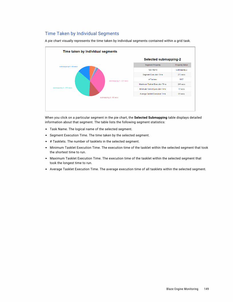
Time Taken by Individual SegmentsA pie chart visually represents the time taken by individual segments contained within a grid task.
When you click on a particular segment in the pie chart, the Selected Submapping table displays detailed information about that segment. The table lists the following segment statistics:
• Task Name. The logical name of the selected segment.
• Segment Execution Time. The time taken by the selected segment.
• # Tasklets. The number of tasklets in the selected segment.
• Minimum Tasklet Execution Time. The execution time of the tasklet within the selected segment that took the shortest time to run.
• Maximum Tasklet Execution Time. The execution time of the tasklet within the selected segment that took the longest time to run.
• Average Tasklet Execution Time. The average execution time of all tasklets within the selected segment.
Blaze Engine Monitoring 149
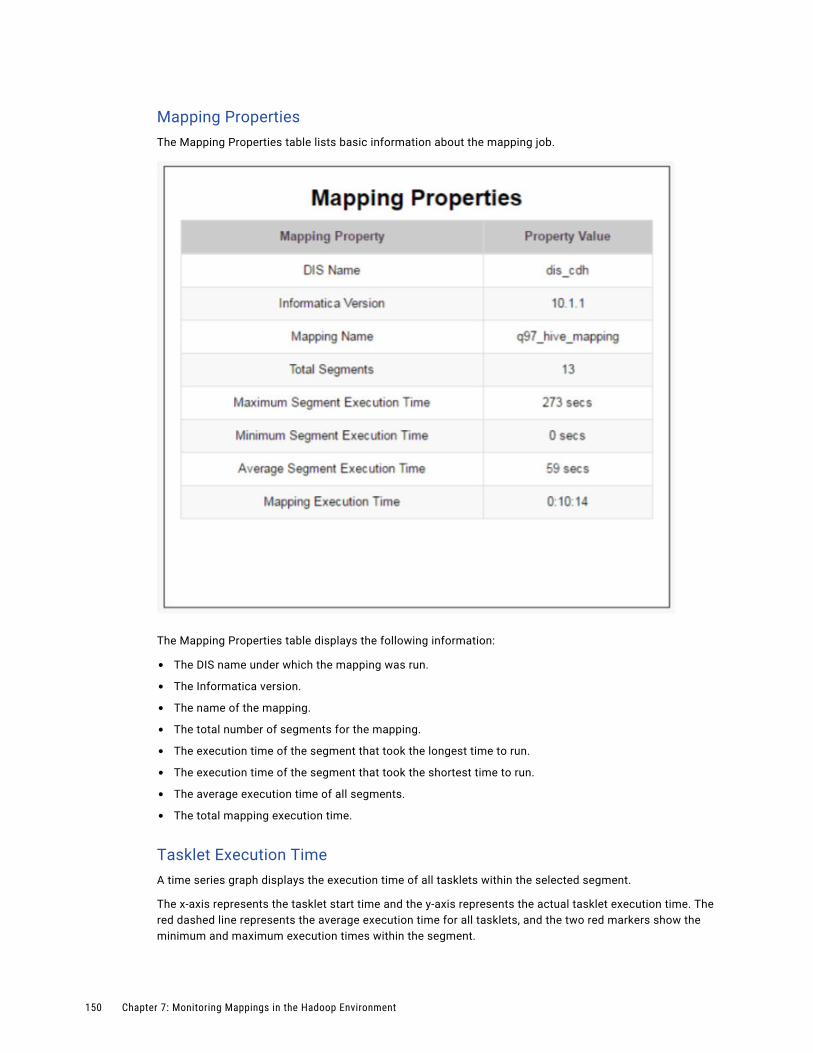
Mapping PropertiesThe Mapping Properties table lists basic information about the mapping job.
The Mapping Properties table displays the following information:
• The DIS name under which the mapping was run.
• The Informatica version.
• The name of the mapping.
• The total number of segments for the mapping.
• The execution time of the segment that took the longest time to run.
• The execution time of the segment that took the shortest time to run.
• The average execution time of all segments.
• The total mapping execution time.
Tasklet Execution TimeA time series graph displays the execution time of all tasklets within the selected segment.
The x-axis represents the tasklet start time and the y-axis represents the actual tasklet execution time. The red dashed line represents the average execution time for all tasklets, and the two red markers show the minimum and maximum execution times within the segment.
150 Chapter 7: Monitoring Mappings in the Hadoop Environment
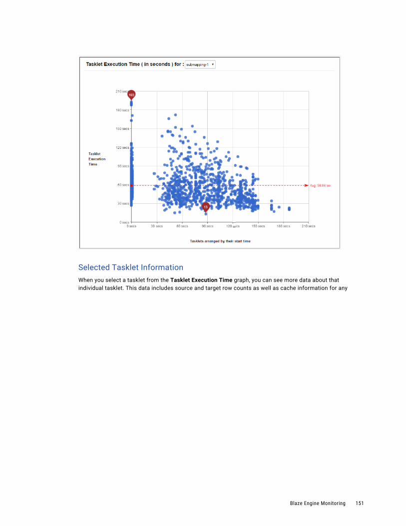
Selected Tasklet InformationWhen you select a tasklet from the Tasklet Execution Time graph, you can see more data about that individual tasklet. This data includes source and target row counts as well as cache information for any
Blaze Engine Monitoring 151
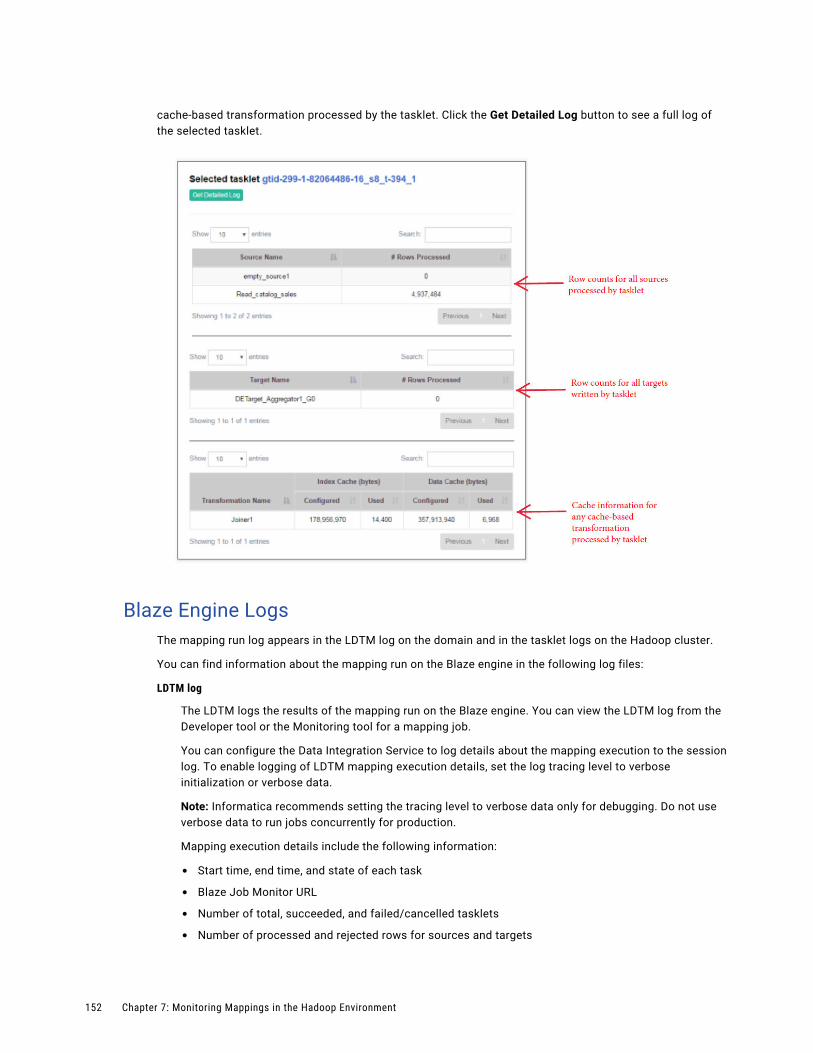
cache-based transformation processed by the tasklet. Click the Get Detailed Log button to see a full log of the selected tasklet.
Blaze Engine LogsThe mapping run log appears in the LDTM log on the domain and in the tasklet logs on the Hadoop cluster.
You can find information about the mapping run on the Blaze engine in the following log files:
LDTM log
The LDTM logs the results of the mapping run on the Blaze engine. You can view the LDTM log from the Developer tool or the Monitoring tool for a mapping job.
You can configure the Data Integration Service to log details about the mapping execution to the session log. To enable logging of LDTM mapping execution details, set the log tracing level to verbose initialization or verbose data.
Note: Informatica recommends setting the tracing level to verbose data only for debugging. Do not use verbose data to run jobs concurrently for production.
Mapping execution details include the following information:
• Start time, end time, and state of each task
• Blaze Job Monitor URL
• Number of total, succeeded, and failed/cancelled tasklets
• Number of processed and rejected rows for sources and targets
152 Chapter 7: Monitoring Mappings in the Hadoop Environment
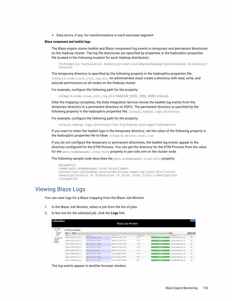
• Data errors, if any, for transformations in each executed segment
Blaze component and tasklet logs
The Blaze engine stores tasklet and Blaze component log events in temporary and permanent directories on the Hadoop cluster. The log file directories are specified by properties in the hadoopEnv.properties file located in the following location for each Hadoop distribution:
<Informatica Installation directory>/services/shared/hadoop/<distribution directory>/infaConf
The temporary directory is specified by the following property in the hadoopEnv.properties file: infagrid.node.local.root.log.dir. An administrator must create a directory with read, write, and execute permissions on all nodes on the Hadoop cluster.
For example, configure the following path for the property:
infagrid.node.local.root.log.dir=$HADOOP_NODE_INFA_HOME/dtmLogsAfter the mapping completes, the Data Integration Service moves the tasklet log events from the temporary directory to a permanent directory on HDFS. The permanent directory is specified by the following property in the hadoopEnv.properties file: infacal.hadoop.logs.directory.
For example, configure the following path for the property:
infacal.hadoop.logs.directory=/var/log/hadoop-yarn/apps/informaticaIf you want to retain the tasklet logs in the temporary directory, set the value of the following property in the hadoopEnv.properties file to false: infagrid.delete.local.log
If you do not configure the temporary or permanent directories, the tasklet log events appear in the directory configured for the DTM Process. You can get the directory for the DTM Process from the value for the yarn.nodemanager.local-dirs property in yarn-site.xml on the cluster node.
The following sample code describes the yarn.nodemanager.local-dirs property:
<property><name>yarn.nodemanager.local-dirs</name><value>/var/lib/hadoop-yarn/cache/${user.name}/nm-local-dir</value><description>List of directories to store local files.</description></property>
Viewing Blaze LogsYou can view logs for a Blaze mapping from the Blaze Job Monitor.
1. In the Blaze Job Monitor, select a job from the list of jobs.
2. In the row for the selected job, click the Logs link.
The log events appear in another browser window.
Blaze Engine Monitoring 153

Troubleshooting Blaze MonitoringWhen I run a mapping on the Blaze engine and try to view the grid task log, the Blaze Job Monitor does not fetch the full log.The grid task log might be too large. The Blaze Job Monitor can only fetch up to 2 MB of an aggregated log. The first line of the log reports this information and provides the location of the full log on HDFS. Follow the link to HDFS and search for "aggregated logs for grid mapping." The link to the full log contains the grid task number.
The Blaze Job Monitor will not start.Check the Hadoop environment logs to locate the issue. If you do not find an issue, stop the Grid Manager with the infacmd stopBlazeService command and run the mapping again.
The Monitoring URL is not displayed in the Properties view of the Administrator tool.Locate the URL in the YARN log.
A Blaze Job Monitor that has been running for several days loses its connection to the Application Timeline Server on the Hortonworks cluster.The Blaze engine requires a running Application Timeline Server on the cluster. When the Blaze engine starts a mapping run, the Blaze Job Monitor checks the state of the Application Timeline Server. The Grid Manager will start it if it is not running. When the connection to the Application Timeline Server is lost, the Blaze engine attempts to reconnect to it. If the Application Timeline Server stops during a Blaze mapping run, you can restart it by restarting the Grid Manager.
Note: When the Application Timeline Server is configured to run on the cluster by default, the cluster administrator must manually restart it on the cluster.
Spark Engine MonitoringYou can monitor statistics and view log events for a Spark engine mapping job in the Monitor tab of the Administrator tool. You can also monitor mapping jobs for the Spark engine in the YARN web user interface.
The following image shows the Monitor tab in the Administrator tool:
154 Chapter 7: Monitoring Mappings in the Hadoop Environment
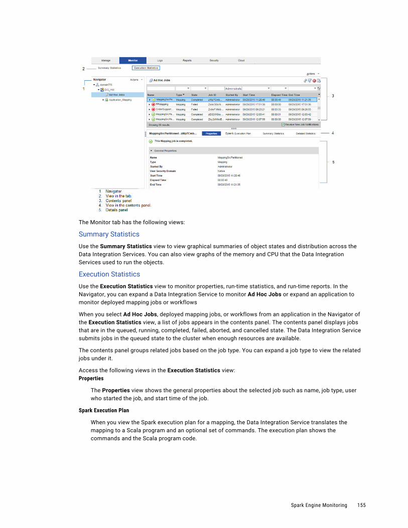
The Monitor tab has the following views:
Summary Statistics
Use the Summary Statistics view to view graphical summaries of object states and distribution across the Data Integration Services. You can also view graphs of the memory and CPU that the Data Integration Services used to run the objects.
Execution Statistics
Use the Execution Statistics view to monitor properties, run-time statistics, and run-time reports. In the Navigator, you can expand a Data Integration Service to monitor Ad Hoc Jobs or expand an application to monitor deployed mapping jobs or workflows
When you select Ad Hoc Jobs, deployed mapping jobs, or workflows from an application in the Navigator of the Execution Statistics view, a list of jobs appears in the contents panel. The contents panel displays jobs that are in the queued, running, completed, failed, aborted, and cancelled state. The Data Integration Service submits jobs in the queued state to the cluster when enough resources are available.
The contents panel groups related jobs based on the job type. You can expand a job type to view the related jobs under it.
Access the following views in the Execution Statistics view:Properties
The Properties view shows the general properties about the selected job such as name, job type, user who started the job, and start time of the job.
Spark Execution Plan
When you view the Spark execution plan for a mapping, the Data Integration Service translates the mapping to a Scala program and an optional set of commands. The execution plan shows the commands and the Scala program code.
Spark Engine Monitoring 155

Summary Statistics
The Summary Statistics view appears in the details panel when you select a mapping job in the contents panel. The Summary Statistics view displays the following throughput statistics for the job:
• Source. The name of the mapping source file.
• Target name. The name of the target file.
• Rows. The number of rows read for source and target.
The following image shows the Summary Statistics view in the details panel for a mapping run on the Spark engine:
Detailed Statistics
The Detailed Statistics view appears in the details panel when you select a mapping job in the contents panel. The Detailed Statistics view displays a graph of the row count for the job run.
The following image shows the Detailed Statistics view in the details panel for a mapping run on the Spark engine:
156 Chapter 7: Monitoring Mappings in the Hadoop Environment
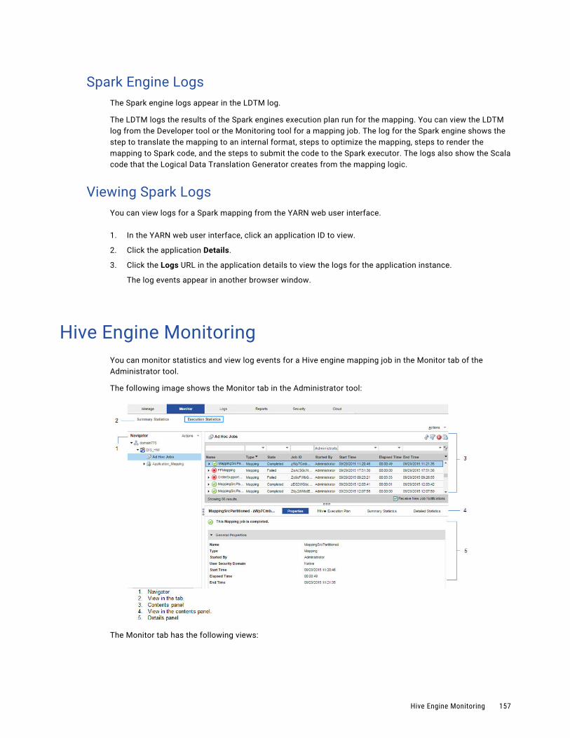
Spark Engine LogsThe Spark engine logs appear in the LDTM log.
The LDTM logs the results of the Spark engines execution plan run for the mapping. You can view the LDTM log from the Developer tool or the Monitoring tool for a mapping job. The log for the Spark engine shows the step to translate the mapping to an internal format, steps to optimize the mapping, steps to render the mapping to Spark code, and the steps to submit the code to the Spark executor. The logs also show the Scala code that the Logical Data Translation Generator creates from the mapping logic.
Viewing Spark LogsYou can view logs for a Spark mapping from the YARN web user interface.
1. In the YARN web user interface, click an application ID to view.
2. Click the application Details.
3. Click the Logs URL in the application details to view the logs for the application instance.
The log events appear in another browser window.
Hive Engine MonitoringYou can monitor statistics and view log events for a Hive engine mapping job in the Monitor tab of the Administrator tool.
The following image shows the Monitor tab in the Administrator tool:
The Monitor tab has the following views:
Hive Engine Monitoring 157
Summary Statistics
Use the Summary Statistics view to view graphical summaries of object states and distribution across the Data Integration Services. You can also view graphs of the memory and CPU that the Data Integration Services used to run the objects.
Execution Statistics
Use the Execution Statistics view to monitor properties, run-time statistics, and run-time reports. In the Navigator, you can expand a Data Integration Service to monitor Ad Hoc Jobs or expand an application to monitor deployed mapping jobs or workflows
When you select Ad Hoc Jobs, deployed mapping jobs, or workflows from an application in the Navigator of the Execution Statistics view, a list of jobs appears in the contents panel. The contents panel displays jobs that are in the queued, running, completed, failed, aborted, and cancelled state. The Data Integration Service submits jobs in the queued state to the cluster when resources are available.
The contents panel groups related jobs based on the job type. You can expand a job type to view the related jobs under it.
Access the following views in the Execution Statistics view:Properties
The Properties view shows the general properties about the selected job such as name, job type, user who started the job, and start time of the job.
Hive Execution Plan
The Hive execution plan displays the Hive script that the Data Integration Service generates based on the mapping logic. The execution plan includes the Hive queries and Hive commands. Each script has a unique identifier.
Summary Statistics
The Summary Statistics view appears in the details panel when you select a mapping job in the contents panel. The Summary Statistics view displays throughput and resource usage statistics for the job.
You can view the following throughput statistics for the job:
• Source. The name of the mapping source file.
• Target name. The name of the target file.
• Rows. The number of rows read for source and target. If the target is Hive, this is the only summary statistic available.
• Average Rows/Sec. Average number of rows read per second for source and target.
• Bytes. Number of bytes read for source and target.
• Average Bytes/Sec. Average number of bytes read per second for source and target.
• First Row Accessed. The date and time when the Data Integration Service started reading the first row in the source file.
• Dropped rows. Number of source rows that the Data Integration Service did not read.
The Hive summary statistics include a row called "AllHiveSourceTables" This row includes records read from the following sources:
• Original Hive sources in the mapping.
• Staging Hive tables defined by the Hive engine.
• Staging data between two linked MapReduce jobs in each query.
158 Chapter 7: Monitoring Mappings in the Hadoop Environment
If the LDTM session includes one MapReduce job, the "AllHiveSourceTables" statistic only includes original Hive sources in the mapping.
Detailed Statistics
The Detailed Statistics view appears in the details panel when you select a mapping job in the contents panel. The Detailed Statistics view displays graphs of the throughput and resource usage statistics for the job run.
Hive Engine LogsThe Hive engine logs appear in the LDTM log and the Hive session log.
You can find the information about Hive engine log events in the following log files:
LDTM log
The LDTM logs the results of the Hive queries run for the mapping. You can view the LDTM log from the Developer tool or the Administrator tool for a mapping job.
Hive session log
For every Hive script in the Hive execution plan for a mapping, the Data Integration Service opens a Hive session to run the Hive queries. A Hive session updates a log file in the following directory on the Data Integration Service node: <InformaticaInstallationDir>/tomcat/bin/disTemp/. The full path to the Hive session log appears in the LDTM log.
Hive Engine Monitoring 159
C h a p t e r 8
Mappings in the Native Environment
This chapter includes the following topics:
• Mappings in the Native Environment Overview, 160
• Data Processor Mappings, 160
• HDFS Mappings, 161
• Hive Mappings, 162
• Social Media Mappings, 163
Mappings in the Native Environment OverviewYou can run a mapping in the native environment. In the native environment, the Data Integration Service runs the mapping from the Developer tool. You can run standalone mappings or mappings that are a part of a workflow.
In the native environment, you can read and process data from large unstructured and semi-structured files, Hive, or social media web sites. You can include the following objects in the mappings:
• Hive sources
• Flat file sources or targets in the local system or in HDFS
• Complex file sources in the local system or in HDFS
• Data Processor transformations to process unstructured and semi-structured file formats
• Social media sources
Data Processor MappingsThe Data Processor transformation processes unstructured and semi-structured file formats in a mapping. It converts source data to flat CSV records that MapReduce applications can process.
You can configure the Data Processor transformation to process messaging formats, HTML pages, XML, and PDF documents. You can also configure it to transform structured formats such as ACORD, HIPAA, HL7, EDI-X12, EDIFACT, AFP, and SWIFT.
160
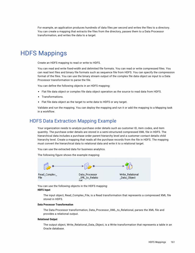
For example, an application produces hundreds of data files per second and writes the files to a directory. You can create a mapping that extracts the files from the directory, passes them to a Data Processor transformation, and writes the data to a target.
HDFS MappingsCreate an HDFS mapping to read or write to HDFS.
You can read and write fixed-width and delimited file formats. You can read or write compressed files. You can read text files and binary file formats such as sequence file from HDFS. You can specify the compression format of the files. You can use the binary stream output of the complex file data object as input to a Data Processor transformation to parse the file.
You can define the following objects in an HDFS mapping:
• Flat file data object or complex file data object operation as the source to read data from HDFS.
• Transformations.
• Flat file data object as the target to write data to HDFS or any target.
Validate and run the mapping. You can deploy the mapping and run it or add the mapping to a Mapping task in a workflow.
HDFS Data Extraction Mapping ExampleYour organization needs to analyze purchase order details such as customer ID, item codes, and item quantity. The purchase order details are stored in a semi-structured compressed XML file in HDFS. The hierarchical data includes a purchase order parent hierarchy level and a customer contact details child hierarchy level. Create a mapping that reads all the purchase records from the file in HDFS. The mapping must convert the hierarchical data to relational data and write it to a relational target.
You can use the extracted data for business analytics.
The following figure shows the example mapping:
You can use the following objects in the HDFS mapping:HDFS Input
The input object, Read_Complex_File, is a Read transformation that represents a compressed XML file stored in HDFS.
Data Processor Transformation
The Data Processor transformation, Data_Processor_XML_to_Relational, parses the XML file and provides a relational output.
Relational Output
The output object, Write_Relational_Data_Object, is a Write transformation that represents a table in an Oracle database.
HDFS Mappings 161
When you run the mapping, the Data Integration Service reads the file in a binary stream and passes it to the Data Processor transformation. The Data Processor transformation parses the specified file and provides a relational output. The output is written to the relational target.
You can configure the mapping to run in a native or Hadoop run-time environment.
Complete the following tasks to configure the mapping:
1. Create an HDFS connection to read files from the Hadoop cluster.
2. Create a complex file data object read operation. Specify the following parameters:
• The file as the resource in the data object.
• The file compression format.
• The HDFS file location.
3. Optionally, you can specify the input format that the Mapper uses to read the file.
4. Drag and drop the complex file data object read operation into a mapping.
5. Create a Data Processor transformation. Configure the following properties in the Data Processor transformation:
• An input port set to buffer input and binary data type.
• Relational output ports depending on the number of columns you want in the relational output. Specify the port size for the ports. Use an XML schema reference that describes the XML hierarchy. Specify the normalized output that you want. For example, you can specify PurchaseOrderNumber_Key as a generated key that relates the Purchase Orders output group to a Customer Details group.
• Create a Streamer object and specify Streamer as a startup component.
6. Create a relational connection to an Oracle database.
7. Import a relational data object.
8. Create a write transformation for the relational data object and add it to the mapping.
Hive MappingsBased on the mapping environment, you can read data from or write data to Hive.
In a native environment, you can read data from Hive. To read data from Hive, complete the following steps:
1. Create a Hive connection.
2. Configure the Hive connection mode to access Hive as a source or target.
3. Use the Hive connection to create a data object to read from Hive.
4. Add the data object to a mapping and configure the mapping to run in the native environment.
You can write to Hive in a Hadoop environment. To write data to Hive, complete the following steps:
1. Create a Hive connection.
2. Configure the Hive connection mode to access Hive as a source or target.
3. Use the Hive connection to create a data object to write to Hive.
4. Add the data object to a mapping and configure the mapping to run in the Hadoop environment.
162 Chapter 8: Mappings in the Native Environment

You can define the following types of objects in a Hive mapping:
• A Read Transformation to read data from Hive
• Transformations
• A target or an SQL data service. You can write to Hive if you run the mapping in a Hadoop cluster.
Validate and run the mapping. You can deploy the mapping and run it or add the mapping to a Mapping task in a workflow.
Hive Mapping ExampleYour organization, HypoMarket Corporation, needs to analyze customer data. Create a mapping that reads all the customer records. Create an SQL data service to make a virtual database available for end users to query.
You can use the following objects in a Hive mapping:Hive input
The input file is a Hive table that contains the customer names and contact details.
Create a relational data object. Configure the Hive connection and specify the table that contains the customer data as a resource for the data object. Drag the data object into a mapping as a read data object.
SQL Data Service output
Create an SQL data service in the Developer tool. To make it available to end users, include it in an application, and deploy the application to a Data Integration Service. When the application is running, connect to the SQL data service from a third-party client tool by supplying a connect string.
You can run SQL queries through the client tool to access the customer data.
Social Media MappingsCreate mappings to read social media data from sources such as Facebook and LinkedIn.
You can extract social media data and load them to a target in the native environment only. You can choose to parse this data or use the data for data mining and analysis.
To process or analyze the data in Hadoop, you must first move the data to a relational or flat file target and then run the mapping in the Hadoop cluster.
You can use the following Informatica adapters in the Developer tool:
• PowerExchange for DataSift
• PowerExchange for Facebook
• PowerExchange for LinkedIn
• PowerExchange for Twitter
• PowerExchange for Web Content-Kapow Katalyst
Review the respective PowerExchange adapter documentation for more information.
Social Media Mappings 163
Twitter Mapping ExampleYour organization, Hypomarket Corporation, needs to review all the tweets that mention your product HypoBasket with a positive attitude since the time you released the product in February 2012.
Create a mapping that identifies tweets that contain the word HypoBasket and writes those records to a table.
You can use the following objects in a Twitter mapping:Twitter input
The mapping source is a Twitter data object that contains the resource Search.
Create a physical data object and add the data object to the mapping. Add the Search resource to the physical data object. Modify the query parameter with the following query:
QUERY=HypoBasket:)&since:2012-02-01Sorter transformation
Optionally, sort the data based on the timestamp.
Add a Sorter transformation to the mapping. Specify the timestamp as the sort key with direction as ascending.
Mapping output
Add a relational data object to the mapping as a target.
After you run the mapping, Data Integration Service writes the extracted tweets to the target table. You can use text analytics and sentiment analysis tools to analyze the tweets.
164 Chapter 8: Mappings in the Native Environment

C h a p t e r 9
ProfilesThis chapter includes the following topics:
• Profiles Overview, 165
• Native Environment, 165
• Hadoop Environment, 166
• Creating a Single Data Object Profile in Informatica Developer, 167
• Creating an Enterprise Discovery Profile in Informatica Developer, 168
• Creating a Column Profile in Informatica Analyst, 169
• Creating an Enterprise Discovery Profile in Informatica Analyst, 170
• Creating a Scorecard in Informatica Analyst, 171
• Monitoring a Profile, 172
• Troubleshooting, 172
Profiles OverviewYou can create and run column profiles, enterprise discovery profiles, and scorecards in the native run-time environment or Hadoop run-time environment.
When you create or edit a profile or scorecard, you can choose the run-time environment. After you choose the run-time environment, the Developer tool or the Analyst tool sets the run-time environment in the profile definition. To process the profiles quickly, you can choose the Hadoop run-time environment.
Native EnvironmentIn Informatica Developer, you can run single object profiles, multiple object profiles, and enterprise discovery profiles in the native environment. In Informatica Analyst, you can run column profiles, enterprise discovery profiles, and scorecards in the native environment.
When you run a profile in the native run-time environment, the Analyst tool or Developer tool submits the profile jobs to the Profiling Service Module. The Profiling Service Module then breaks down the profile jobs into a set of mappings. The Data Integration Service runs these mappings on the same machine where the Data Integration Service runs and writes the profile results to the profiling warehouse. By default, all profiles run in the native run-time environment.
165

You can use native sources to create and run profiles in the native environment. A native data source is a non-Hadoop source, such as a flat file, relational source, or mainframe source. You can also run a profile on a mapping specification or a logical data source with a Hive or HDFS data source in the native environment.
Hadoop EnvironmentYou can run profiles and scorecards in the Hadoop environment on the Hive engine or Blaze engine. You can choose Hive or Hadoop option to run the profiles in the Hadoop run-time environment. After you choose the Hive option and select a Hadoop connection, the Data Integration Service pushes the profile logic to the Hive engine on the Hadoop cluster to run profiles. After you choose the Hadoop option and select a Hadoop connection, the Data Integration Service pushes the profile logic to the Blaze engine on the Hadoop cluster to run profiles.
When you run a profile in the Hadoop environment, the Analyst tool submits the profile jobs to the Profiling Service Module. The Profiling Service Module then breaks down the profile jobs into a set of mappings. The Data Integration Service pushes the mappings to the Hadoop environment through the Hadoop connection. The Hive engine or Blaze engine processes the mappings and the Data Integration Service writes the profile results to the profiling warehouse.
In the Developer tool, you can run single object profiles and multiple object profiles, and enterprise discovery profiles on the Blaze engine. In the Analyst tool, you can run column profiles, enterprise discovery profiles, and scorecards on the Blaze engine.
Column Profiles for Sqoop Data SourcesYou can run a column profile on data objects that use Sqoop. You can select the Hive or Hadoop run-time environment to run the column profiles.
On the Hive engine, to run a column profile on a relational data object that uses Sqoop, you must set the Sqoop argument m to 1 in the JDBC connection. Use the following syntax:
-m 1
When you run a column profile on a logical data object or customized data object, you can configure the num-mappers argument to achieve parallelism and optimize performance. You must also configure the split-by argument to specify the column based on which Sqoop must split the work units.
Use the following syntax:
--split-by <column_name>
If the primary key does not have an even distribution of values between the minimum and maximum range, you can configure the split-by argument to specify another column that has a balanced distribution of data to split the work units.
If you do not define the split-by column, Sqoop splits work units based on the following criteria:
• If the data object contains a single primary key, Sqoop uses the primary key as the split-by column.
• If the data object contains a composite primary key, Sqoop defaults to the behavior of handling composite primary keys without the split-by argument. See the Sqoop documentation for more information.
• If a data object contains two tables with an identical column, you must define the split-by column with a table-qualified name. For example, if the table name is CUSTOMER and the column name is FULL_NAME, define the split-by column as follows:--split-by CUSTOMER.FULL_NAME
166 Chapter 9: Profiles
• If the data object does not contain a primary key, the value of the m argument and num-mappers argument default to 1.
When you use the Cloudera Connector Powered by Teradata or Hortonworks Connector for Teradata and the Teradata table does not contain a primary key, the split-by argument is required.
Creating a Single Data Object Profile in Informatica Developer
You can create a single data object profile for one or more columns in a data object and store the profile object in the Model repository.
1. In the Object Explorer view, select the data object you want to profile.
2. Click File > New > Profile to open the profile wizard.
3. Select Profile and click Next.
4. Enter a name for the profile and verify the project location. If required, browse to a new location.
5. Optionally, enter a text description of the profile.
6. Verify that the name of the data object you selected appears in the Data Objects section.
7. Click Next.
8. Configure the profile operations that you want to perform. You can configure the following operations:
• Column profiling
• Primary key discovery
• Functional dependency discovery
• Data domain discovery
Note: To enable a profile operation, select Enabled as part of the "Run Profile" action for that operation. Column profiling is enabled by default.
9. Review the options for your profile.
You can edit the column selection for all profile types. Review the filter and sampling options for column profiles. You can review the inference options for primary key, functional dependency, and data domain discovery. You can also review data domain selection for data domain discovery.
10. Review the drill-down options, and edit them if necessary. By default, the Enable Row Drilldown option is selected. You can edit drill-down options for column profiles. The options also determine whether drill-down operations read from the data source or from staged data, and whether the profile stores result data from previous profile runs.
11. In the Run Settings section, choose a run-time environment. Choose Native, Hive, or Hadoop as the run-time environment. When you choose the Hive or Hadoop option, select a Hadoop connection.
12. Click Finish.
Creating a Single Data Object Profile in Informatica Developer 167

Creating an Enterprise Discovery Profile in Informatica Developer
You can create a profile on multiple data sources under multiple connections. The Developer tool creates individual profile tasks for each source.
1. In the Object Explorer view, select multiple data objects you want to run a profile on.
2. Click File > New > Profile to open the profile wizard.
3. Select Enterprise Discovery Profile and click Next.
4. Enter a name for the profile and verify the project location. If required, browse to a new location.
5. Verify that the name of the data objects you selected appears within the Data Objects section. Click Choose to select more data objects, if required.
6. Click Next.
The Add Resources to Profile Definition pane appears. You can select multiple, external relational connections and data sources from this pane.
7. Click Choose to open the Select Resources dialog box.
The Resources pane lists all the internal and external connections and data objects under the Informatica domain.
8. Click OK to close the dialog box.
9. Click Next.
10. Configure the profile types that you want to run. You can configure the following profile types:
• Data domain discovery
• Column profile
• Primary key profile
• Foreign key profile
Note: Select Enabled as part of "Run Enterprise Discovery Profile" action for the profile types that you want to run as part of the enterprise discovery profile. Column profiling is enabled by default.
11. Review the options for the profile.
You can edit the sampling options for column profiles. You can also edit the inference options for data domain, primary key, and foreign key profiles.
12. Select Create profiles.
The Developer tool creates profiles for each individual data source.
13. Select Run enterprise discovery profile on finish to run the profile when you complete the profile configuration. If you enabled all the profiling operations, the Developer tool runs column, data domain, and primary key profiles on all selected data sources. Then, the Developer tool runs a foreign key profile across all the data sources.
14. Click Finish.
After you run an enterprise discovery profile, you need to refresh the Model Repository Service before viewing the results. This step is required as the import of metadata for external connections happens in the Model repository. You need to refresh the Model Repository Service so that the Developer tool reflects the changes to the Model repository.
168 Chapter 9: Profiles
Creating a Column Profile in Informatica AnalystYou can create a custom profile or default profile. When you create a custom profile, you can configure the columns, sample rows, and drill-down options. When you create a default profile, the column profile and data domain discovery runs on the entire data set with all the data domains.
1. In the Discovery workspace, click Profile, or select New > Profile from the header area.
Note: You can right-click on the data object in the Library workspace and create a profile. In this profile, the profile name, location name, and data object are extracted from the data object properties. You can create a default profile or customize the settings to create a custom profile.
The New Profile wizard appears.
2. The Single source option is selected by default. Click Next.
3. In the Specify General Properties screen, enter a name and an optional description for the profile. In the Location field, select the project or folder where you want to create the profile. Click Next.
4. In the Select Source screen, click Choose to select a data object, or click New to import a data object. Click Next.
• In the Choose Data Object dialog box, select a data object. Click OK.The Properties pane displays the properties of the selected data object. The Data Preview pane displays the columns in the data object.
• In the New Data Object dialog box, you can choose a connection, schema, table, or view to create a profile on, select a location, and create a folder to import the data object. Click OK.
5. In the Select Source screen, select the columns that you want to run a profile on. Optionally, select Name to select all the columns. Click Next.
All the columns are selected by default. The Analyst tool lists column properties, such as the name, data type, precision, scale, nullable, and participates in the primary key for each column.
6. In the Specify Settings screen, choose to run a column profile, data domain discovery, or a column profile and data domain discovery. By default, column profile option is selected.
• Choose Run column profile to run a column profile.
• Choose Run data domain discovery to perform data domain discovery. In the Data domain pane, select the data domains that you want to discover, select a conformance criteria, and select the columns for data domain discovery in the Edit columns selection for data domin discovery dialog box.
• Choose Run column profile and Run data domain discovery to run the column profile and data domain discovery. Select the data domain options in the Data domain pane.
Note: By default, the columns that you select is for column profile and data domain discovery. Click Edit to select or deselect columns for data domain discovery.
• Choose Data, Columns, or Data and Columns to run data domain discovery on.
• Choose a sampling option. You can choose All rows (complete analysis), Sample first, Random sample , or Random sample (auto) as a sampling option in the Run profile on pane. This option applies to column profile and data domain discovery.
• Choose a drilldown option. You can choose Live or Staged drilldown option, or you can choose Off to disable drilldown in the Drilldown pane. Optionally, click Select Columns to select columns to drill down on. You can choose to omit data type and data domain inference for columns with an approved data type or data domain.
Creating a Column Profile in Informatica Analyst 169
• Choose Native, Hive, or Hadoop option as the run-time environment. If you choose the Hive or Hadoop option, click Choose to select a Hadoop connection in the Select a Hadoop Connection dialog box.
7. Click Next.
The Specify Rules and Filters screen opens.
8. In the Specify Rules and Filters screen, you can perform the following tasks:
• Create, edit, or delete a rule. You can apply existing rules to the profile.
• Create, edit, or delete a filter.
Note: When you create a scorecard on this profile, you can reuse the filters that you create for the profile.
9. Click Save and Finish to create the profile, or click Save and Run to create and run the profile.
Creating an Enterprise Discovery Profile in Informatica Analyst
You can run column profile and data domain discovery as part of enterprise discovery in Informatica Analyst.
1. In the Discovery workspace, select New > Profile.
The New Profile wizard appears.
2. Select Enterprise Discovery . Click Next.
The Specify General Properties tab appears.
3. In the Specify General Properties tab, enter a name for the enterprise discovery profile and an optional description. In the Location field, select the project or folder where you want to create the profile. Click Next.
The Select Data Objects tab appears.
4. In the Select Data Objects tab, click Choose.
The Choose Data objects dialog box appears.
5. In the Choose Data objects dialog box, choose one or more data objects to add to the profile. Click Save.
The data objects appear in the Data Objects pane.
6. Click Next.
The Select Resources tab appears.
7. In the Select Resources tab, click Choose to open the Select Resources tab.
You can import data from multiple relational data sources.
8. In the Select Resources tab, select the connections, schemas, tables, and views that you want to include in the profile. Click Save.
The left pane in the dialog box lists all the internal and external connections, schemas, tables, and views under the Informatica domain.
The resources appear in the Resource pane.
9. Click Next.
The Specify Settings tab appears.
170 Chapter 9: Profiles
10. In the Specify Settings tab, you can configure the column profile options and data domain discovery options. Click Save and Finish to save the enterprise discovery profile, or click Save and Run to run the profile.
You can perform the following tasks in the Specify Settings tab.
• Enable data domain discovery. Click Choose to select data domains that you want to discover from the Choose Data Domains dialog box. The selected data domains appear in the Data Domains for Data Domain Discovery pane.
• Run data domain on data, column name, or on both data and column name.
• Select all the rows in the data source, or choose a maximum number of rows to run domain discovery on.
• Choose a minimum conformance percentage or specify the minimum number of conforming rows for data domain discovery.
• Enable column profile settings and select all rows or first few rows in the data source for the column profile. You can exclude data type inference for columns with approved data types in the column profile.
• Choose Native or Hadoop as the run-time environment.
You can view the enterprise discovery results under the Summary and Profiles tabs.
Creating a Scorecard in Informatica AnalystCreate a scorecard and add columns from a profile to the scorecard. You must run a profile before you add columns to the scorecard.
1. In the Library workspace, select the project or folder that contains the profile.
2. Click the profile to open the profile.
The profile results appear in the summary view in the Discovery workspace.
3. Click Actions > Add to scorecard.
The Add to Scorecard wizard appears.
4. In the Add to Scorecard screen, you can choose to create a new scorecard, or edit an existing scorecard to add the columns to a predefined scorecard. The New Scorecard option is selected by default. Click Next.
5. In the Step 2 of 8 screen, enter a name for the scorecard. Optionally, you can enter a description for the scorecard. Select the project and folder where you want to save the scorecard. Click Next.
By default, the scorecard wizard selects the columns and rules defined in the profile. You cannot add columns that are not included in the profile.
6. In the Step 3 of 8 screen, select the columns and rules that you want to add to the scorecard as metrics. Optionally, click the check box in the left column header to select all columns. Optionally, select Column Name to sort column names. Click Next.
7. In the Step 4 of 8 screen, you can add a filter to the metric.
You can apply the filter that you created for the profile to the metrics, or create a new filter. Select a metric in the Metric Filters pane, and click the Manage Filters icon to open the Edit Filter: column name dialog box. In the Edit Filter: column name dialog box, you can choose to perform one of the following tasks:
Creating a Scorecard in Informatica Analyst 171
• You can choose a filter that you created for the profile. Click Next.
• Select an existing filter. Click edit icon to edit the filter in the Edit Filter dialog box. Click Next.
• Click the plus (+) icon to create filters in the New Filter dialog box. Click Next.
The filter appears in the Metric Filters pane. You can apply the same filter to all the metrics in the scorecard.
8. In the Step 4 of 8 screen, click Next.
9. In the Step 5 of 8 screen, select each metric in the Metrics pane and configure the valid values from the list of all values in the Score using: Values pane. You can perform the following tasks in the Step 5 of 7 screen:
• You can select multiple values in the Available Values pane, and click the right arrow button to move them to the Valid Values pane. The total number of valid values for a metric appears at the top of the Available Values pane.
• In the Metric Thresholds pane, configure metric thresholds.
You can set thresholds for Good, Acceptable, and Unacceptable scores.
• Select each metric and configure the cost of invalid data. To assign a constant value to the cost for the metric, select Fixed Cost. Optionally, click Change Cost Unit to change the unit of cost or choose None. To attach a numeric column as a variable cost to the metric, select Variable Cost, and click Select Column to select a numeric column.
10. In the Step 6 of 8 screen, you can select a metric group to which you can add the metrics, or create a new metric group, To create a new metric group, click the group icon. Click Next.
11. In the Step 7 of 8 screen, specify the weights for the metrics in the group and thresholds for the group.
12. In the Step 8 of 8 screen, select Native or Hadoop as the run-time environment to run the scorecard.
13. Click Save to save the scorecard, or click Save & Run to save and run the scorecard.
The scorecard appears in the Scorecard workspace.
Monitoring a ProfileYou can monitor a profile in the Administrator tool.
1. In the Administrator tool, click the Monitor tab.
2. In the Navigator workspace, select Jobs.
3. Select a profiling job.
4. In the Summary Statistics tab, you can view the general properties of the profile, summary statistics, and detailed statistics of the profile.
5. Click the Execution Statistics tab to view execution statistics for the profile.
TroubleshootingCan I drill down on profile results if I run a profile in the Hadoop environment?
Yes, except for profiles in which you have set the option to drill down on staged data.
172 Chapter 9: Profiles
I get the following error message when I run a profile in the Hadoop environment: “[LDTM_1055] The Integration Service failed to generate a Hive workflow for mapping [Profile_CUSTOMER_INFO12_14258652520457390]." How do I resolve this?
This error can result from a data source, rule transformation, or run-time environment that is not supported in the Hadoop environment. For more information about objects that are not valid in the Hadoop environment, see the Mappings in a Hadoop Environment chapter.
You can change the data source, rule, or run-time environment and run the profile again. View the profile log file for more information on the error.
I see "N/A" in the profile results for all columns after I run a profile. How do I resolve this?
Verify that the profiling results are in the profiling warehouse. If you do not see the profile results, verify that the database path is accurate in the HadoopEnv.properties file. You can also verify the database path from the Hadoop job tracker on the Monitoring tab of the Administrator tool.
After I run a profile on a Hive source, I do not see the results. When I verify the Hadoop job tracker, I see the following error when I open the profile job: "XML Parsing Error: no element found." What does this mean?
The Hive data source does not have any record and is empty. The data source must have a minimum of one row of data for successful profile run.
After I run a profile on a Hive source, I cannot view some of the column patterns. Why?
When you import a Hive source, the Developer tool sets the precision for string columns to 4000. The Developer tool cannot derive the pattern for a string column with a precision greater than 255. To resolve this issue, set the precision of these string columns in the data source to 255 and run the profile again.
When I run a profile on large Hadoop sources, the profile job fails and I get an "execution failed" error. What can be the possible cause?
One of the causes can be a connection issue. Perform the following steps to identify and resolve the connection issue:
1. Open the Hadoop job tracker.
2. Identify the profile job and open it to view the MapReduce jobs.
3. Click the hyperlink for the failed job to view the error message. If the error message contains the text "java.net.ConnectException: Connection refused", the problem occured because of an issue with the Hadoop cluster. Contact your network administrator to resolve the issue.
Troubleshooting 173
C h a p t e r 1 0
Native Environment OptimizationThis chapter includes the following topics:
• Native Environment Optimization Overview, 174
• Processing Big Data on a Grid, 174
• Processing Big Data on Partitions, 175
• High Availability, 176
Native Environment Optimization OverviewYou can optimize the native environment to increase performance. To increase performance, you can configure the Data Integration Service to run on a grid and to use multiple partitions to process data. You can also enable high availability to ensure that the domain can continue running despite temporary network, hardware, or service failures.
You can run profiles, sessions, and workflows on a grid to increase the processing bandwidth. A grid is an alias assigned to a group of nodes that run profiles, sessions, and workflows. When you enable grid, the Data Integration Service runs a service process on each available node of the grid to increase performance and scalability.
You can also run mapping with partitioning to increase performance. When you run a partitioned session or a partitioned mapping, the Data Integration Service performs the extract, transformation, and load for each partition in parallel.
You can configure high availability for the domain. High availability eliminates a single point of failure in a domain and provides minimal service interruption in the event of failure.
Processing Big Data on a GridYou can run an Integration Service on a grid to increase the processing bandwidth. When you enable grid, the Integration Service runs a service process on each available node of the grid to increase performance and scalability.
Big data may require additional bandwidth to process large amounts of data. For example, when you run a Model repository profile on an extremely large data set, the Data Integration Service grid splits the profile into multiple mappings and runs the mappings simultaneously on different nodes in the grid.
174

Data Integration Service GridYou can run Model repository mappings and profiles on a Data Integration Service grid.
When you run mappings on a grid, the Data Integration Service distributes the mappings to multiple DTM processes on nodes in the grid. When you run a profile on a grid, the Data Integration Service splits the profile into multiple mappings and distributes the mappings to multiple DTM processes on nodes in the grid.
For more information about the Data Integration Service grid, see the Informatica Administrator Guide.
Grid OptimizationYou can optimize the grid to increase performance and scalability of the Data Integration Service.
To optimize the grid, complete the following task:
Add nodes to the grid.
Add nodes to the grid to increase processing bandwidth of the Data Integration Service.
Processing Big Data on PartitionsYou can run a Model repository mapping with partitioning to increase performance. When you run a mapping configured with partitioning, the Data Integration Service performs the extract, transformation, and load for each partition in parallel.
Mappings that process large data sets can take a long time to process and can cause low data throughput. When you configure partitioning, the Data Integration Service uses additional threads to process the session or mapping which can increase performance.
Partitioned Model Repository MappingsYou can enable the Data Integration Service to use multiple partitions to process Model repository mappings.
If the nodes where mappings run have multiple CPUs, you can enable the Data Integration Service to maximize parallelism when it runs mappings. When you maximize parallelism, the Data Integration Service dynamically divides the underlying data into partitions and processes all of the partitions concurrently.
Optionally, developers can set a maximum parallelism value for a mapping in the Developer tool. By default, the maximum parallelism for each mapping is set to Auto. Each mapping uses the maximum parallelism value defined for the Data Integration Service. Developers can change the maximum parallelism value in the mapping run-time properties to define a maximum value for a particular mapping. When maximum parallelism is set to different integer values for the Data Integration Service and the mapping, the Data Integration Service uses the minimum value.
For more information, see the Informatica Application Services Guide and the Informatica Developer Mapping Guide.
Processing Big Data on Partitions 175
Partition OptimizationYou can optimize the partitioning of Model repository mappings to increase performance. You can add more partitions, select the best performing partition types, use more CPUs, and optimize the source or target database for partitioning.
To optimize partitioning, perform the following tasks:
Increase the number of partitions.
When you configure Model repository mappings, you increase the number of partitions when you increase the maximum parallelism value for the Data Integration Service or the mapping.
Increase the number of partitions to enable the Data Integration Service to create multiple connections to sources and process partitions of source data concurrently. Increasing the number of partitions increases the number of threads, which also increases the load on the Data Integration Service nodes. If the Data Integration Service node or nodes contain ample CPU bandwidth, processing rows of data concurrently can increase performance.
Note: If you use a single-node Data Integration Service and the Data Integration Service uses a large number of partitions in a session or mapping that processes large amounts of data, you can overload the system.
Use multiple CPUs.
If you have a symmetric multi-processing (SMP) platform, you can use multiple CPUs to concurrently process partitions of data.
Optimize the source database for partitioning.
You can optimize the source database for partitioning. For example, you can tune the database, enable parallel queries, separate data into different tablespaces, and group sorted data.
Optimize the target database for partitioning.
You can optimize the target database for partitioning. For example, you can enable parallel inserts into the database, separate data into different tablespaces, and increase the maximum number of sessions allowed to the database.
High AvailabilityHigh availability eliminates a single point of failure in an Informatica domain and provides minimal service interruption in the event of failure. When you configure high availability for a domain, the domain can continue running despite temporary network, hardware, or service failures. You can configure high availability for the domain, application services, and application clients.
The following high availability components make services highly available in an Informatica domain:
• Resilience. An Informatica domain can tolerate temporary connection failures until either the resilience timeout expires or the failure is fixed.
• Restart and failover. A process can restart on the same node or on a backup node after the process becomes unavailable.
• Recovery. Operations can complete after a service is interrupted. After a service process restarts or fails over, it restores the service state and recovers operations.
When you plan a highly available Informatica environment, consider the differences between internal Informatica components and systems that are external to Informatica. Internal components include the
176 Chapter 10: Native Environment Optimization

Service Manager, application services, and command line programs. External systems include the network, hardware, database management systems, FTP servers, message queues, and shared storage.
High availability features for the Informatica environment are available based on your license.
High Availability 177
A p p e n d i x A
Data Type ReferenceThis appendix includes the following topics:
• Data Type Reference Overview, 178
• Transformation Data Type Support in a Hadoop Environment, 179
• Complex File and Transformation Data Types, 179
• Hive Data Types and Transformation Data Types, 183
• Sqoop Data Types, 185
Data Type Reference OverviewInformatica Developer uses the following data types in mappings that run on the Hadoop cluster:Native data types
Native data types are specific to the Hadoop sources and targets used as a physical data object. Native data types appear in the physical data object column properties.
Transformation data types
Transformation data types are set of data types that appear in the transformations. They are internal data types based on ANSI SQL-92 generic data types, which the Data Integration Service uses to move data across platforms. Transformation data types appear in all transformations in a mapping.
Transformation data types include the following data types:
• Primitive data type. Represents a single data value in a single column position.
• Complex data type. Represents multiple data values in a single column position. Use complex data types in mappings that run on the Spark engine to process hierarchical data in complex files.
When the Data Integration Service reads source data, it converts the native data types to the comparable transformation data types before transforming the data. When the Data Integration Service writes to a target, it converts the transformation data types to the comparable native data types.
178
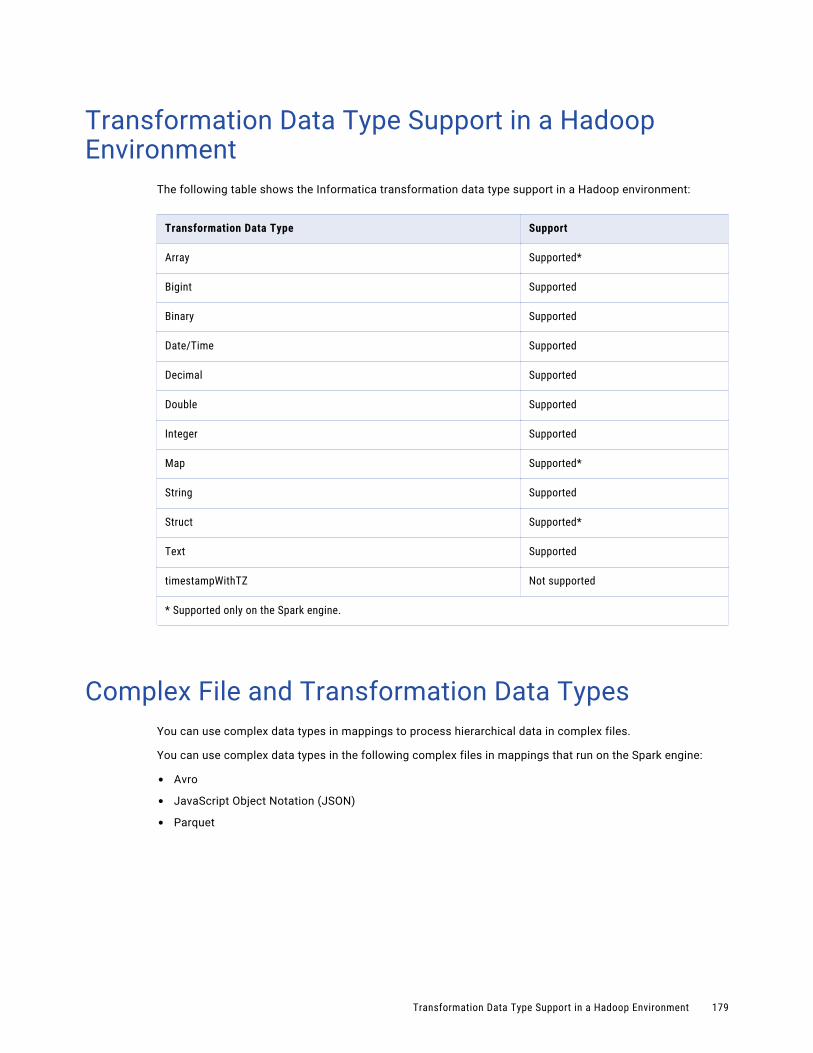
Transformation Data Type Support in a Hadoop Environment
The following table shows the Informatica transformation data type support in a Hadoop environment:
Transformation Data Type Support
Array Supported*
Bigint Supported
Binary Supported
Date/Time Supported
Decimal Supported
Double Supported
Integer Supported
Map Supported*
String Supported
Struct Supported*
Text Supported
timestampWithTZ Not supported
* Supported only on the Spark engine.
Complex File and Transformation Data TypesYou can use complex data types in mappings to process hierarchical data in complex files.
You can use complex data types in the following complex files in mappings that run on the Spark engine:
• Avro
• JavaScript Object Notation (JSON)
• Parquet
Transformation Data Type Support in a Hadoop Environment 179
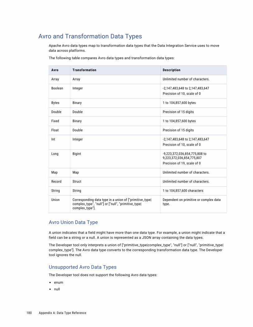
Avro and Transformation Data TypesApache Avro data types map to transformation data types that the Data Integration Service uses to move data across platforms.
The following table compares Avro data types and transformation data types:
Avro Transformation Description
Array Array Unlimited number of characters.
Boolean Integer -2,147,483,648 to 2,147,483,647Precision of 10, scale of 0
Bytes Binary 1 to 104,857,600 bytes
Double Double Precision of 15 digits
Fixed Binary 1 to 104,857,600 bytes
Float Double Precision of 15 digits
Int Integer -2,147,483,648 to 2,147,483,647Precision of 10, scale of 0
Long Bigint -9,223,372,036,854,775,808 to 9,223,372,036,854,775,807Precision of 19, scale of 0
Map Map Unlimited number of characters.
Record Struct Unlimited number of characters.
String String 1 to 104,857,600 characters
Union Corresponding data type in a union of ["primitive_type|complex_type", "null"] or ["null", "primitive_type|complex_type"].
Dependent on primitive or complex data type.
Avro Union Data Type
A union indicates that a field might have more than one data type. For example, a union might indicate that a field can be a string or a null. A union is represented as a JSON array containing the data types.
The Developer tool only interprets a union of ["primitive_type|complex_type", "null"] or ["null", "primitive_type|complex_type"]. The Avro data type converts to the corresponding transformation data type. The Developer tool ignores the null.
Unsupported Avro Data TypesThe Developer tool does not support the following Avro data types:
• enum
• null
180 Appendix A: Data Type Reference

JSON and Transformation Data TypesJavaScript Object Notation data types map to transformation data types that the Data Integration Service uses to move data across platforms.
The following table compares JSON data types and transformation data types:
JSON Transformation Description
Array Array Unlimited number of characters.
Double Double Precision of 15 digits
Integer Integer -2,147,483,648 to 2,147,483,647Precision of 10, scale of 0
Object Struct Unlimited number of characters.
String String 1 to 104,857,600 characters
Unsupported JSON Data TypesThe Developer tool does not support the following JSON data types:
• date/timestamp
• enum
• union
Parquet and Transformation Data TypesApache Parquet data types map to transformation data types that the Data Integration Service uses to move data across platforms.
The following table compares Parquet data types and transformation data types:
Parquet Transformation Description
Binary Binary 1 to 104,857,600 bytes
Binary (UTF8) String 1 to 104,857,600 characters
Boolean Integer -2,147,483,648 to 2,147,483,647Precision of 10, scale of 0
Double Double Precision of 15 digits
Complex File and Transformation Data Types 181
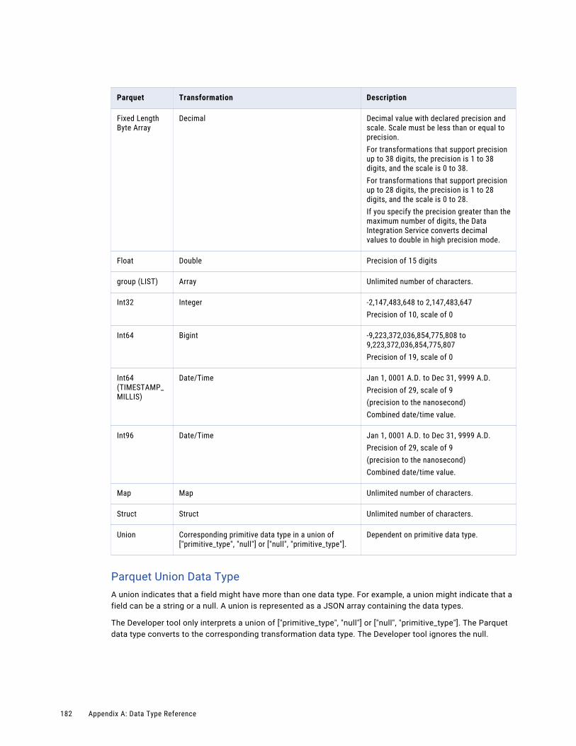
Parquet Transformation Description
Fixed Length Byte Array
Decimal Decimal value with declared precision and scale. Scale must be less than or equal to precision.For transformations that support precision up to 38 digits, the precision is 1 to 38 digits, and the scale is 0 to 38. For transformations that support precision up to 28 digits, the precision is 1 to 28 digits, and the scale is 0 to 28. If you specify the precision greater than the maximum number of digits, the Data Integration Service converts decimal values to double in high precision mode.
Float Double Precision of 15 digits
group (LIST) Array Unlimited number of characters.
Int32 Integer -2,147,483,648 to 2,147,483,647Precision of 10, scale of 0
Int64 Bigint -9,223,372,036,854,775,808 to 9,223,372,036,854,775,807Precision of 19, scale of 0
Int64 (TIMESTAMP_MILLIS)
Date/Time Jan 1, 0001 A.D. to Dec 31, 9999 A.D.Precision of 29, scale of 9(precision to the nanosecond)Combined date/time value.
Int96 Date/Time Jan 1, 0001 A.D. to Dec 31, 9999 A.D.Precision of 29, scale of 9(precision to the nanosecond)Combined date/time value.
Map Map Unlimited number of characters.
Struct Struct Unlimited number of characters.
Union Corresponding primitive data type in a union of ["primitive_type", "null"] or ["null", "primitive_type"].
Dependent on primitive data type.
Parquet Union Data TypeA union indicates that a field might have more than one data type. For example, a union might indicate that a field can be a string or a null. A union is represented as a JSON array containing the data types.
The Developer tool only interprets a union of ["primitive_type", "null"] or ["null", "primitive_type"]. The Parquet data type converts to the corresponding transformation data type. The Developer tool ignores the null.
182 Appendix A: Data Type Reference
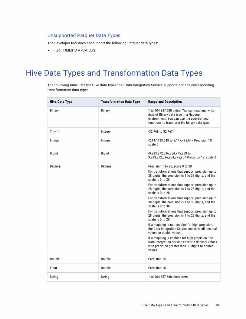
Unsupported Parquet Data TypesThe Developer tool does not support the following Parquet data types:
• int96 (TIMESTAMP_MILLIS)
Hive Data Types and Transformation Data TypesThe following table lists the Hive data types that Data Integration Service supports and the corresponding transformation data types:
Hive Data Type Transformation Data Type Range and Description
Binary Binary 1 to 104,857,600 bytes. You can read and write data of Binary data type in a Hadoop environment. You can use the user-defined functions to transform the binary data type.
Tiny Int Integer -32,768 to 32,767
Integer Integer -2,147,483,648 to 2,147,483,647 Precision 10, scale 0
Bigint Bigint -9,223,372,036,854,775,808 to 9,223,372,036,854,775,807 Precision 19, scale 0
Decimal Decimal Precision 1 to 28, scale 0 to 28For transformations that support precision up to 38 digits, the precision is 1 to 38 digits, and the scale is 0 to 38. For transformations that support precision up to 28 digits, the precision is 1 to 28 digits, and the scale is 0 to 28. For transformations that support precision up to 38 digits, the precision is 1 to 38 digits, and the scale is 0 to 38. For transformations that support precision up to 28 digits, the precision is 1 to 28 digits, and the scale is 0 to 28. If a mapping is not enabled for high precision, the Data Integration Service converts all decimal values to double values.If a mapping is enabled for high precision, the Data Integration Service converts decimal values with precision greater than 38 digits to double values.
Double Double Precision 15
Float Double Precision 15
String String 1 to 104,857,600 characters
Hive Data Types and Transformation Data Types 183
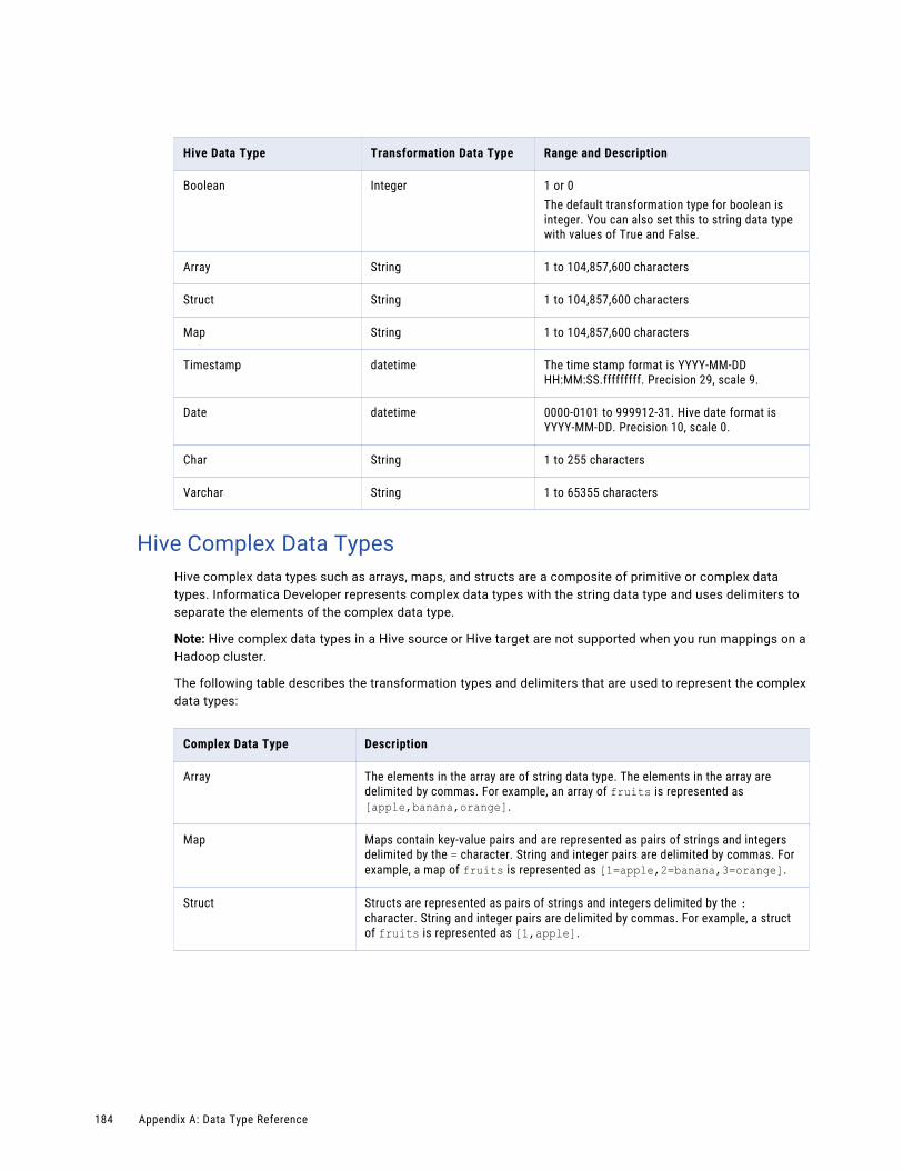
Hive Data Type Transformation Data Type Range and Description
Boolean Integer 1 or 0The default transformation type for boolean is integer. You can also set this to string data type with values of True and False.
Array String 1 to 104,857,600 characters
Struct String 1 to 104,857,600 characters
Map String 1 to 104,857,600 characters
Timestamp datetime The time stamp format is YYYY-MM-DD HH:MM:SS.fffffffff. Precision 29, scale 9.
Date datetime 0000-0101 to 999912-31. Hive date format is YYYY-MM-DD. Precision 10, scale 0.
Char String 1 to 255 characters
Varchar String 1 to 65355 characters
Hive Complex Data TypesHive complex data types such as arrays, maps, and structs are a composite of primitive or complex data types. Informatica Developer represents complex data types with the string data type and uses delimiters to separate the elements of the complex data type.
Note: Hive complex data types in a Hive source or Hive target are not supported when you run mappings on a Hadoop cluster.
The following table describes the transformation types and delimiters that are used to represent the complex data types:
Complex Data Type Description
Array The elements in the array are of string data type. The elements in the array are delimited by commas. For example, an array of fruits is represented as [apple,banana,orange].
Map Maps contain key-value pairs and are represented as pairs of strings and integers delimited by the = character. String and integer pairs are delimited by commas. For example, a map of fruits is represented as [1=apple,2=banana,3=orange].
Struct Structs are represented as pairs of strings and integers delimited by the : character. String and integer pairs are delimited by commas. For example, a struct of fruits is represented as [1,apple].
184 Appendix A: Data Type Reference
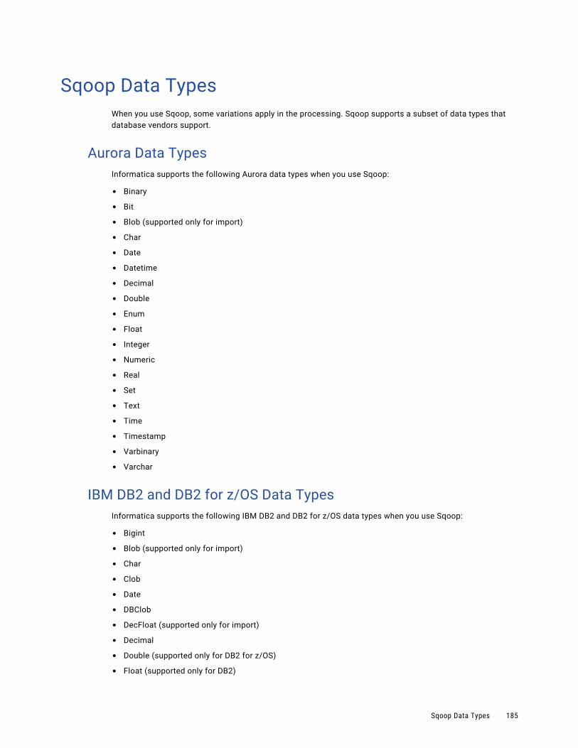
Sqoop Data TypesWhen you use Sqoop, some variations apply in the processing. Sqoop supports a subset of data types that database vendors support.
Aurora Data TypesInformatica supports the following Aurora data types when you use Sqoop:
• Binary
• Bit
• Blob (supported only for import)
• Char
• Date
• Datetime
• Decimal
• Double
• Enum
• Float
• Integer
• Numeric
• Real
• Set
• Text
• Time
• Timestamp
• Varbinary
• Varchar
IBM DB2 and DB2 for z/OS Data TypesInformatica supports the following IBM DB2 and DB2 for z/OS data types when you use Sqoop:
• Bigint
• Blob (supported only for import)
• Char
• Clob
• Date
• DBClob
• DecFloat (supported only for import)
• Decimal
• Double (supported only for DB2 for z/OS)
• Float (supported only for DB2)
Sqoop Data Types 185
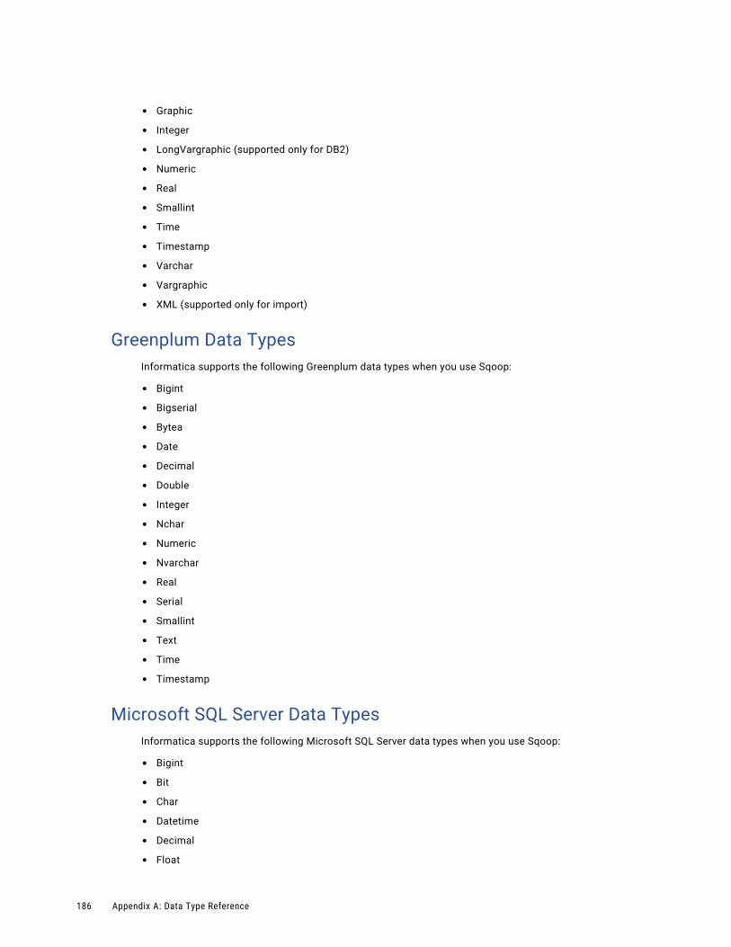
• Graphic
• Integer
• LongVargraphic (supported only for DB2)
• Numeric
• Real
• Smallint
• Time
• Timestamp
• Varchar
• Vargraphic
• XML (supported only for import)
Greenplum Data TypesInformatica supports the following Greenplum data types when you use Sqoop:
• Bigint
• Bigserial
• Bytea
• Date
• Decimal
• Double
• Integer
• Nchar
• Numeric
• Nvarchar
• Real
• Serial
• Smallint
• Text
• Time
• Timestamp
Microsoft SQL Server Data TypesInformatica supports the following Microsoft SQL Server data types when you use Sqoop:
• Bigint
• Bit
• Char
• Datetime
• Decimal
• Float
186 Appendix A: Data Type Reference

• INT
• Money
• Numeric
• Real
• Smalldatetime
• Smallint
• Smallmoney
• Text
• Time
• Tinyint
• Varchar
Rules and Guidelines for Sqoop Microsoft SQL Server Data Types
Consider the following rules and guidelines when you configure Microsoft SQL Server data types in a Sqoop mapping:
• If you create or replace the target table at run time and run the mapping on the Blaze or Spark engine to export Bigint data, the mapping fails.
• If you run a Sqoop mapping to export time data, Sqoop does not export milliseconds.
Netezza Data TypesInformatica supports the following Netezza data types when you use Sqoop:
• Bigint
• Blob (supported only for import)
• Byteint
• Char
• Date
• Double
• Float4
• Float8
• Number
• Timestamp
• Varchar
Oracle Data TypesInformatica supports the following Oracle data types when you use Sqoop:
• Blob (supported only for import)
• Char
• Date
• Float
• Long
Sqoop Data Types 187
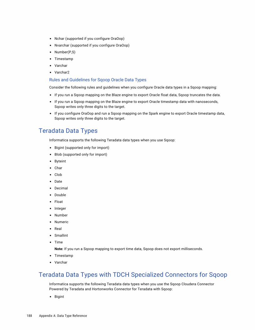
• Nchar (supported if you configure OraOop)
• Nvarchar (supported if you configure OraOop)
• Number(P,S)
• Timestamp
• Varchar
• Varchar2
Rules and Guidelines for Sqoop Oracle Data Types
Consider the following rules and guidelines when you configure Oracle data types in a Sqoop mapping:
• If you run a Sqoop mapping on the Blaze engine to export Oracle float data, Sqoop truncates the data.
• If you run a Sqoop mapping on the Blaze engine to export Oracle timestamp data with nanoseconds, Sqoop writes only three digits to the target.
• If you configure OraOop and run a Sqoop mapping on the Spark engine to export Oracle timestamp data, Sqoop writes only three digits to the target.
Teradata Data TypesInformatica supports the following Teradata data types when you use Sqoop:
• Bigint (supported only for import)
• Blob (supported only for import)
• Byteint
• Char
• Clob
• Date
• Decimal
• Double
• Float
• Integer
• Number
• Numeric
• Real
• Smallint
• Time
Note: If you run a Sqoop mapping to export time data, Sqoop does not export milliseconds.
• Timestamp
• Varchar
Teradata Data Types with TDCH Specialized Connectors for SqoopInformatica supports the following Teradata data types when you use the Sqoop Cloudera Connector Powered by Teradata and Hortonworks Connector for Teradata with Sqoop:
• Bigint
188 Appendix A: Data Type Reference

• Byte (supported only by Hortonworks Connector for Teradata)
• Byteint
• Character
• Date
• Decimal
• Double Precision/Float/Real
• Integer
• Number(P,S)
• Numeric
• Smallint
• Time
• Timestamp (supported only by Cloudera Connector Powered by Teradata)
• Varchar
• Varbyte (supported only by Hortonworks Connector for Teradata)
Sqoop Data Types 189
A p p e n d i x B
Complex File Data Object Properties
This appendix includes the following topics:
• Complex File Data Objects Overview, 190
• Creating and Configuring a Complex File Data Object, 190
• Complex File Data Object Overview Properties, 191
• Compression and Decompression for Complex File Sources and Targets, 192
• Parameterization of Complex File Data Objects, 193
• Complex File Data Object Read Properties, 194
• Complex File Data Object Write Properties, 196
Complex File Data Objects OverviewA complex file data object is a representation of a file in the Hadoop Distributed File System (HDFS). Create a complex file data object to read data from or write data to complex files, such as Avro, JSON, and Parquet, in the HDFS.
You can read from complex files on a local system or in the HDFS. Similarly, you can write to complex files on a local system or in the HDFS. To access files in the HDFS, you must use an HDFS connection. When you use an HDFS connection, you can create a complex file data object to read data from a directory of files that have the same format and properties. You can read from and write to compressed complex files.
When you create a complex file data object, the Developer tool creates a read and write operation. Use the complex file data object read operation as a source in mappings and mapplets. Use the complex file data object write operation as a target in mappings and mapplets.
Creating and Configuring a Complex File Data ObjectCreate and configure a complex file data object to read data from or write data to files in the HDFS.
1. Select a project or folder in the Object Explorer view.
2. Click File > New > Data Object.
190
3. Select Complex File Data Object and click Next.
The New Complex File Data Object dialog box appears.
4. Optionally, enter a name for the data object.
5. Click Browse next to the Location option and select the target project or folder.
6. In the Resource Format list, select the file format of the file.
7. In the Access Type list, select one of the following options:
• Connection. To access a file in the HDFS.
• File. To access a file on the local system.
8. If you selected the connection access type, complete the following steps:
a. Click Browse next to the Connection option and select an HDFS connection.
b. Click Add next to the Selected Resource option to add a resource to the data object.
The Add Resource dialog box appears.
c. Navigate or search for the resources to add to the data object and click OK.
The resources you add appear in the Selected Resources list.
9. If you selected the file access type, complete the following steps:
a. Click Browse next to the Resource Location option and select the file that you want to add.
b. Select File to access a file on your local system.
c. Click Fetch.
The file you selected appears in the Selected Resources list.
10. Click Finish.
The data object appears under the Physical Data Objects category in the project or folder in the Object Explorer view. A read and write operation is created for the data object.
11. Based on whether you want to use the complex file data object as a source or target, edit the read or write operation properties.
You can also create multiple read and write operations for a complex file data object.
Complex File Data Object Overview PropertiesThe Data Integration Service uses overview properties when it reads data from or writes data to a complex file.
Overview properties include general properties that apply to the complex file data object. They also include object properties that apply to the resources in the complex file data object. The Developer tool displays overview properties for complex files in the Overview view.
Complex File Data Object Overview Properties 191
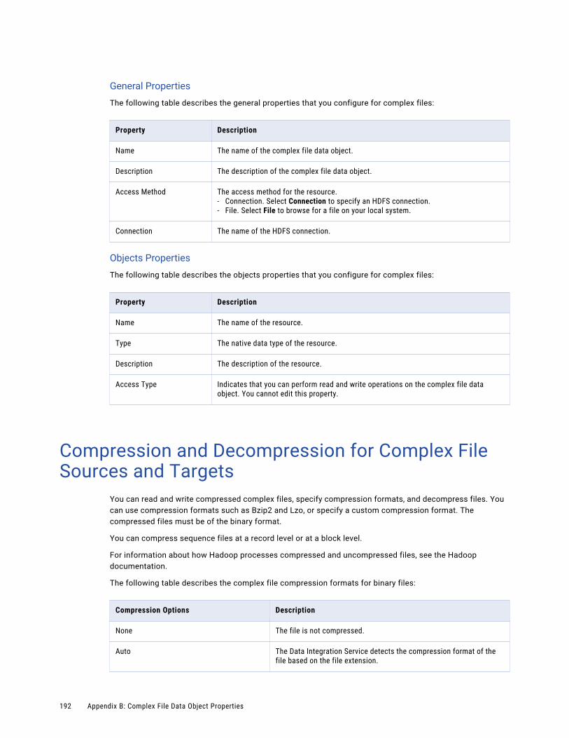
General Properties
The following table describes the general properties that you configure for complex files:
Property Description
Name The name of the complex file data object.
Description The description of the complex file data object.
Access Method The access method for the resource.- Connection. Select Connection to specify an HDFS connection.- File. Select File to browse for a file on your local system.
Connection The name of the HDFS connection.
Objects Properties
The following table describes the objects properties that you configure for complex files:
Property Description
Name The name of the resource.
Type The native data type of the resource.
Description The description of the resource.
Access Type Indicates that you can perform read and write operations on the complex file data object. You cannot edit this property.
Compression and Decompression for Complex File Sources and Targets
You can read and write compressed complex files, specify compression formats, and decompress files. You can use compression formats such as Bzip2 and Lzo, or specify a custom compression format. The compressed files must be of the binary format.
You can compress sequence files at a record level or at a block level.
For information about how Hadoop processes compressed and uncompressed files, see the Hadoop documentation.
The following table describes the complex file compression formats for binary files:
Compression Options Description
None The file is not compressed.
Auto The Data Integration Service detects the compression format of the file based on the file extension.
192 Appendix B: Complex File Data Object Properties

Compression Options Description
DEFLATE The DEFLATE compression format that uses a combination of the LZ77 algorithm and Huffman coding.
Gzip The GNU zip compression format that uses the DEFLATE algorithm.
Bzip2 The Bzip2 compression format that uses the Burrows–Wheeler algorithm.
Lzo The Lzo compression format that uses the Lempel-Ziv-Oberhumer algorithm.
Snappy The LZ77-type compression format with a fixed, byte-oriented encoding.
Custom Custom compression format. If you select this option, you must specify the fully qualified class name implementing the CompressionCodec interface in the Custom Compression Codec field.
Parameterization of Complex File Data ObjectsYou can parameterize the complex file connection and the complex file data object operation properties.
You can parameterize the following data object read operation properties for complex data objects:
• Connection in the run-time properties
• File Format, Input Format, Compression Format, and Custom Compression Codec in the advanced properties.
You can parameterize the following data object write operation properties for complex file data objects:
• Connection in the run-time properties.
• File Name, Output Format, Output Key Class, Output Value Class, Compression Format, Custom Compression Codec, and Sequence File Compression Type in the advanced properties.
The following attributes support full and partial parameterization for complex file data objects:
• File Path in the advanced properties of the data object read operation.For example, to parameterize a part of the attribute value where the file path in the advanced property is /user/adpqa/dynschema.txt, create a parameter as $str="/user/adpqa", and then edit the file path as $str/dynschema.txt. You can also parameterize the value of the entire file path.
• File Directory in the advanced properties of the data object write operation.For example, to parameterize a part of the attribute value where the file directory in the advanced property is /export/home/qamercury/source, create a parameter as $param="/export/home", and then edit the file directory as $param/qamercury/source. You can also parameterize the value of the entire directory.
Parameterization of Complex File Data Objects 193

Complex File Data Object Read PropertiesThe Data Integration Service uses read properties when it reads data from a complex file. Select the Output transformation to edit the general, ports, sources, and run-time properties.Note: The FileName port is displayed by default when you create a data object read operation. You can remove the FileName port if you do not want to read the FileName data.
General PropertiesThe Developer tool displays general properties for complex file sources in the Read view.
The following table describes the general properties that you configure for complex file sources:
Property Description
Name The name of the complex file.This property is read-only. You can edit the name in the Overview view. When you use the complex file as a source in a mapping, you can edit the name in the mapping.
Description The description of the complex file.
Ports PropertiesPorts properties for a physical data object include port names and port attributes such as data type and precision.
Note: The port size specified in the source transformation and Output transformation must be the same.
The following table describes the ports properties that you configure for complex file sources:
Property Description
Name The name of the resource.
Type The native data type of the resource.
Precision The maximum number of significant digits for numeric data types, or the maximum number of characters for string data types.
Description The description of the resource.
Sources PropertiesThe Developer tool displays the sources properties for complex file sources in the Output transformation in the Read view.
The sources properties list the resources of the complex file data object. You can add or remove resources in the data object.
194 Appendix B: Complex File Data Object Properties
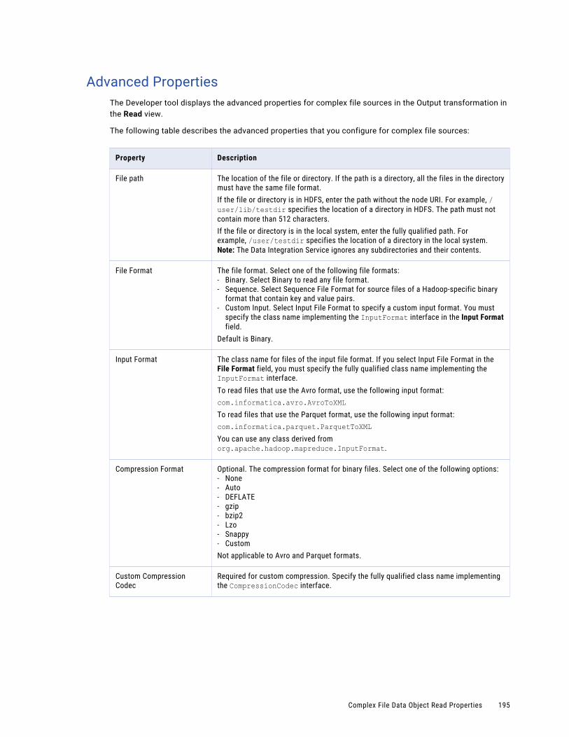
Advanced PropertiesThe Developer tool displays the advanced properties for complex file sources in the Output transformation in the Read view.
The following table describes the advanced properties that you configure for complex file sources:
Property Description
File path The location of the file or directory. If the path is a directory, all the files in the directory must have the same file format.If the file or directory is in HDFS, enter the path without the node URI. For example, /user/lib/testdir specifies the location of a directory in HDFS. The path must not contain more than 512 characters.If the file or directory is in the local system, enter the fully qualified path. For example, /user/testdir specifies the location of a directory in the local system.Note: The Data Integration Service ignores any subdirectories and their contents.
File Format The file format. Select one of the following file formats:- Binary. Select Binary to read any file format.- Sequence. Select Sequence File Format for source files of a Hadoop-specific binary
format that contain key and value pairs.- Custom Input. Select Input File Format to specify a custom input format. You must
specify the class name implementing the InputFormat interface in the Input Format field.
Default is Binary.
Input Format The class name for files of the input file format. If you select Input File Format in the File Format field, you must specify the fully qualified class name implementing the InputFormat interface.To read files that use the Avro format, use the following input format:com.informatica.avro.AvroToXMLTo read files that use the Parquet format, use the following input format:com.informatica.parquet.ParquetToXMLYou can use any class derived from org.apache.hadoop.mapreduce.InputFormat.
Compression Format Optional. The compression format for binary files. Select one of the following options:- None- Auto- DEFLATE- gzip- bzip2- Lzo- Snappy- CustomNot applicable to Avro and Parquet formats.
Custom Compression Codec
Required for custom compression. Specify the fully qualified class name implementing the CompressionCodec interface.
Complex File Data Object Read Properties 195
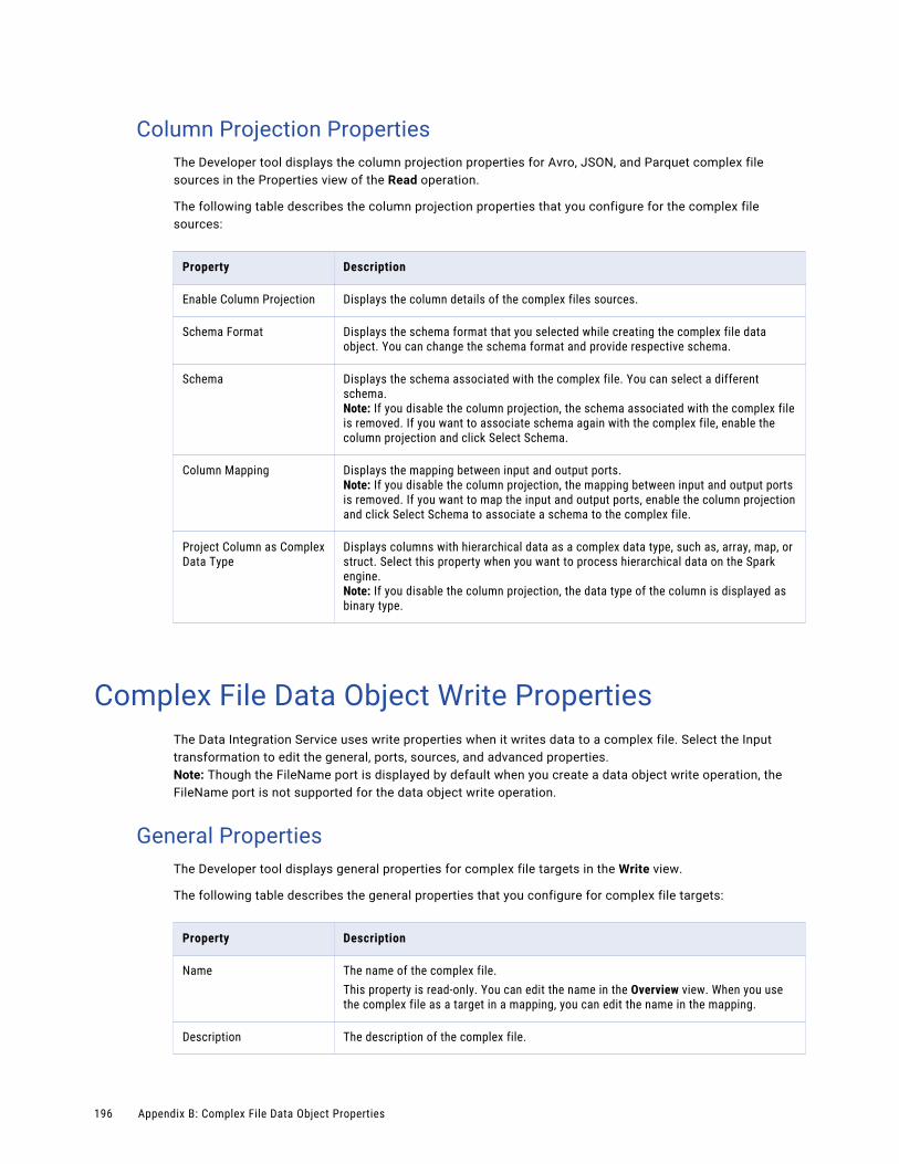
Column Projection PropertiesThe Developer tool displays the column projection properties for Avro, JSON, and Parquet complex file sources in the Properties view of the Read operation.
The following table describes the column projection properties that you configure for the complex file sources:
Property Description
Enable Column Projection Displays the column details of the complex files sources.
Schema Format Displays the schema format that you selected while creating the complex file data object. You can change the schema format and provide respective schema.
Schema Displays the schema associated with the complex file. You can select a different schema.Note: If you disable the column projection, the schema associated with the complex file is removed. If you want to associate schema again with the complex file, enable the column projection and click Select Schema.
Column Mapping Displays the mapping between input and output ports.Note: If you disable the column projection, the mapping between input and output ports is removed. If you want to map the input and output ports, enable the column projection and click Select Schema to associate a schema to the complex file.
Project Column as Complex Data Type
Displays columns with hierarchical data as a complex data type, such as, array, map, or struct. Select this property when you want to process hierarchical data on the Spark engine.Note: If you disable the column projection, the data type of the column is displayed as binary type.
Complex File Data Object Write PropertiesThe Data Integration Service uses write properties when it writes data to a complex file. Select the Input transformation to edit the general, ports, sources, and advanced properties.Note: Though the FileName port is displayed by default when you create a data object write operation, the FileName port is not supported for the data object write operation.
General PropertiesThe Developer tool displays general properties for complex file targets in the Write view.
The following table describes the general properties that you configure for complex file targets:
Property Description
Name The name of the complex file.This property is read-only. You can edit the name in the Overview view. When you use the complex file as a target in a mapping, you can edit the name in the mapping.
Description The description of the complex file.
196 Appendix B: Complex File Data Object Properties
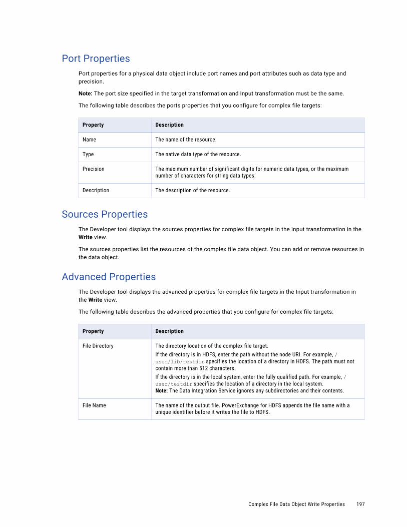
Port PropertiesPort properties for a physical data object include port names and port attributes such as data type and precision.
Note: The port size specified in the target transformation and Input transformation must be the same.
The following table describes the ports properties that you configure for complex file targets:
Property Description
Name The name of the resource.
Type The native data type of the resource.
Precision The maximum number of significant digits for numeric data types, or the maximum number of characters for string data types.
Description The description of the resource.
Sources PropertiesThe Developer tool displays the sources properties for complex file targets in the Input transformation in the Write view.
The sources properties list the resources of the complex file data object. You can add or remove resources in the data object.
Advanced PropertiesThe Developer tool displays the advanced properties for complex file targets in the Input transformation in the Write view.
The following table describes the advanced properties that you configure for complex file targets:
Property Description
File Directory The directory location of the complex file target.If the directory is in HDFS, enter the path without the node URI. For example, /user/lib/testdir specifies the location of a directory in HDFS. The path must not contain more than 512 characters.If the directory is in the local system, enter the fully qualified path. For example, /user/testdir specifies the location of a directory in the local system.Note: The Data Integration Service ignores any subdirectories and their contents.
File Name The name of the output file. PowerExchange for HDFS appends the file name with a unique identifier before it writes the file to HDFS.
Complex File Data Object Write Properties 197
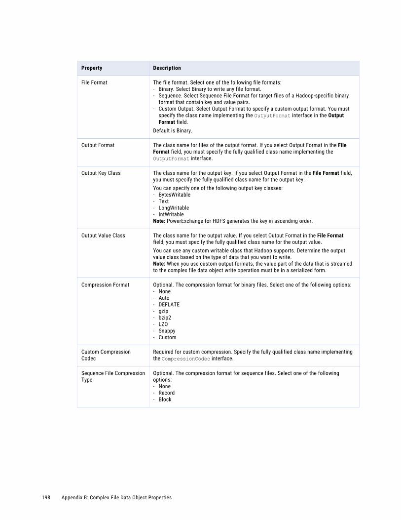
Property Description
File Format The file format. Select one of the following file formats:- Binary. Select Binary to write any file format.- Sequence. Select Sequence File Format for target files of a Hadoop-specific binary
format that contain key and value pairs.- Custom Output. Select Output Format to specify a custom output format. You must
specify the class name implementing the OutputFormat interface in the Output Format field.
Default is Binary.
Output Format The class name for files of the output format. If you select Output Format in the File Format field, you must specify the fully qualified class name implementing the OutputFormat interface.
Output Key Class The class name for the output key. If you select Output Format in the File Format field, you must specify the fully qualified class name for the output key.You can specify one of the following output key classes:- BytesWritable- Text- LongWritable- IntWritableNote: PowerExchange for HDFS generates the key in ascending order.
Output Value Class The class name for the output value. If you select Output Format in the File Format field, you must specify the fully qualified class name for the output value.You can use any custom writable class that Hadoop supports. Determine the output value class based on the type of data that you want to write.Note: When you use custom output formats, the value part of the data that is streamed to the complex file data object write operation must be in a serialized form.
Compression Format Optional. The compression format for binary files. Select one of the following options:- None- Auto- DEFLATE- gzip- bzip2- LZO- Snappy- Custom
Custom Compression Codec
Required for custom compression. Specify the fully qualified class name implementing the CompressionCodec interface.
Sequence File Compression Type
Optional. The compression format for sequence files. Select one of the following options:- None- Record- Block
198 Appendix B: Complex File Data Object Properties
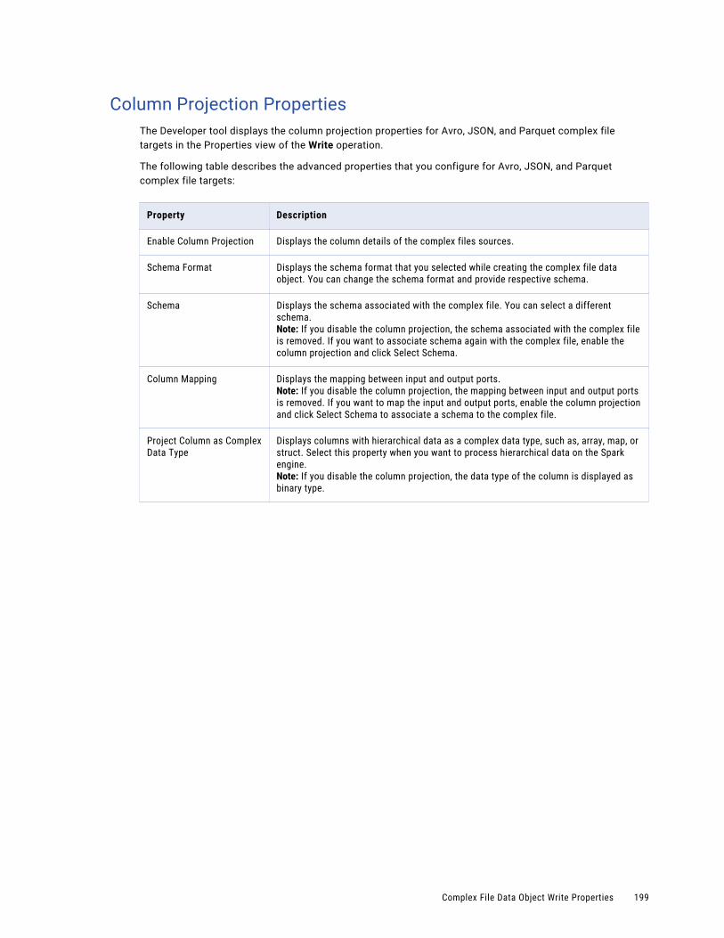
Column Projection PropertiesThe Developer tool displays the column projection properties for Avro, JSON, and Parquet complex file targets in the Properties view of the Write operation.
The following table describes the advanced properties that you configure for Avro, JSON, and Parquet complex file targets:
Property Description
Enable Column Projection Displays the column details of the complex files sources.
Schema Format Displays the schema format that you selected while creating the complex file data object. You can change the schema format and provide respective schema.
Schema Displays the schema associated with the complex file. You can select a different schema.Note: If you disable the column projection, the schema associated with the complex file is removed. If you want to associate schema again with the complex file, enable the column projection and click Select Schema.
Column Mapping Displays the mapping between input and output ports.Note: If you disable the column projection, the mapping between input and output ports is removed. If you want to map the input and output ports, enable the column projection and click Select Schema to associate a schema to the complex file.
Project Column as Complex Data Type
Displays columns with hierarchical data as a complex data type, such as, array, map, or struct. Select this property when you want to process hierarchical data on the Spark engine.Note: If you disable the column projection, the data type of the column is displayed as binary type.
Complex File Data Object Write Properties 199
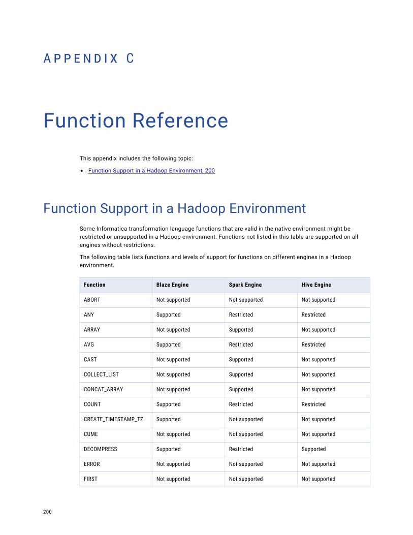
A p p e n d i x C
Function ReferenceThis appendix includes the following topic:
• Function Support in a Hadoop Environment, 200
Function Support in a Hadoop EnvironmentSome Informatica transformation language functions that are valid in the native environment might be restricted or unsupported in a Hadoop environment. Functions not listed in this table are supported on all engines without restrictions.
The following table lists functions and levels of support for functions on different engines in a Hadoop environment.
Function Blaze Engine Spark Engine Hive Engine
ABORT Not supported Not supported Not supported
ANY Supported Restricted Restricted
ARRAY Not supported Supported Not supported
AVG Supported Restricted Restricted
CAST Not supported Supported Not supported
COLLECT_LIST Not supported Supported Not supported
CONCAT_ARRAY Not supported Supported Not supported
COUNT Supported Restricted Restricted
CREATE_TIMESTAMP_TZ Supported Not supported Not supported
CUME Not supported Not supported Not supported
DECOMPRESS Supported Restricted Supported
ERROR Not supported Not supported Not supported
FIRST Not supported Not supported Not supported
200
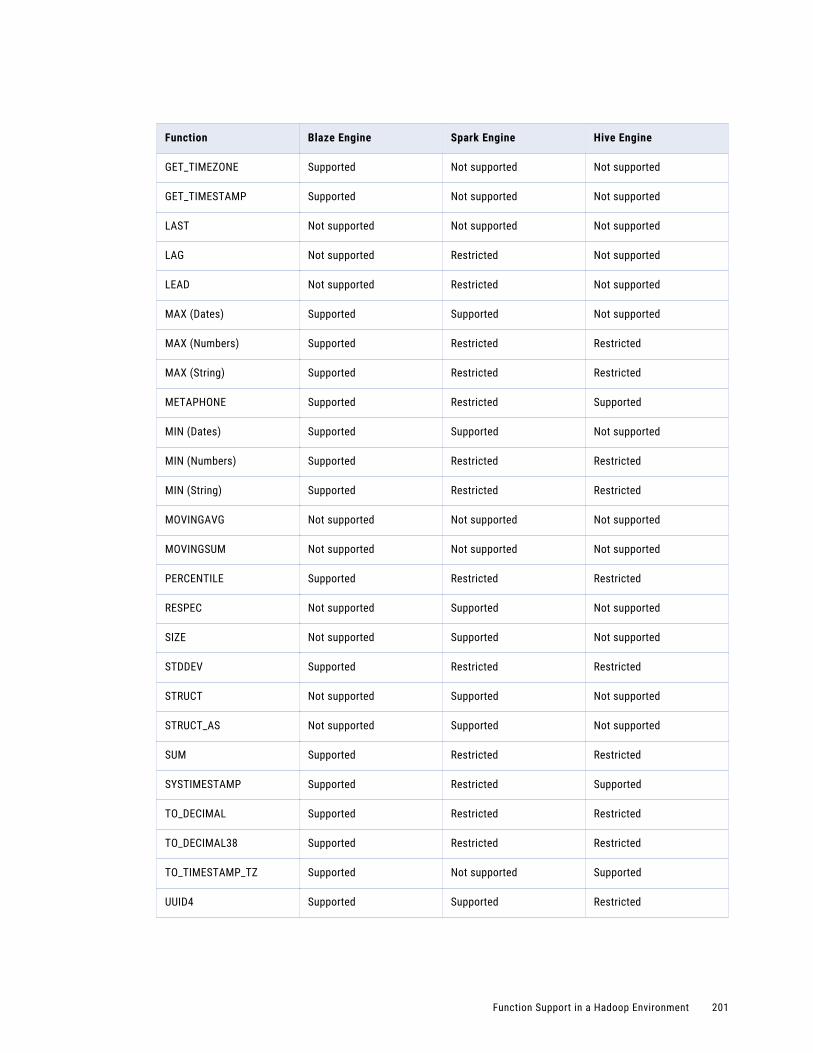
Function Blaze Engine Spark Engine Hive Engine
GET_TIMEZONE Supported Not supported Not supported
GET_TIMESTAMP Supported Not supported Not supported
LAST Not supported Not supported Not supported
LAG Not supported Restricted Not supported
LEAD Not supported Restricted Not supported
MAX (Dates) Supported Supported Not supported
MAX (Numbers) Supported Restricted Restricted
MAX (String) Supported Restricted Restricted
METAPHONE Supported Restricted Supported
MIN (Dates) Supported Supported Not supported
MIN (Numbers) Supported Restricted Restricted
MIN (String) Supported Restricted Restricted
MOVINGAVG Not supported Not supported Not supported
MOVINGSUM Not supported Not supported Not supported
PERCENTILE Supported Restricted Restricted
RESPEC Not supported Supported Not supported
SIZE Not supported Supported Not supported
STDDEV Supported Restricted Restricted
STRUCT Not supported Supported Not supported
STRUCT_AS Not supported Supported Not supported
SUM Supported Restricted Restricted
SYSTIMESTAMP Supported Restricted Supported
TO_DECIMAL Supported Restricted Restricted
TO_DECIMAL38 Supported Restricted Restricted
TO_TIMESTAMP_TZ Supported Not supported Supported
UUID4 Supported Supported Restricted
Function Support in a Hadoop Environment 201

Function Blaze Engine Spark Engine Hive Engine
UUID_UNPARSE Supported Supported Restricted
VARIANCE Supported Restricted Restricted
202 Appendix C: Function Reference
A p p e n d i x D
Parameter ReferenceThis appendix includes the following topics:
• Parameters Overview, 203
• Parameter Usage, 204
Parameters OverviewA mapping parameter represents a constant value that you can change between mapping runs. Use parameters to change the values of connections, file directories, expression components, port lists, port links, and task properties. You can use system parameters or user-defined parameters.
System parameters are built-in parameters for a Data Integration Service. System parameters define the directories where the Data Integration Service stores log files, cache files, reject files, source files, target files, and temporary files. An administrator defines the system parameter default values for a Data Integration Service in the Administrator tool.
User-defined parameters are parameters that you define in transformations, mappings, or workflows. Create user-defined parameters to rerun a mapping with different connection, flat file, cache file, temporary file, expression, ports, or reference table values.
You can override parameter values using a parameter set or a parameter file. A parameter set is a repository object that contains mapping parameter values. A parameter file is an XML file that contains parameter values. When you run the mapping with a parameter set or a parameter file, the Data Integration Service uses the parameter values defined in the parameter set or parameter file instead of the default parameter values you configured in the transformation, mapping, or workflow.
You can use the following parameters to represent additional properties in the Hadoop environment:
Parameters for sources and targets
You can use parameters to represent additional properties for the following big data sources and targets:
• Complex file
• Flat file
• HBase
• HDFS
• Hive
Parameters for the Hadoop connection and run-time environment
You can set the Hive version, run-time environment, and Hadoop connection with a parameter.
203
For more information about mapping parameters, see the Informatica Developer Mapping Guide.
Parameter UsageUse parameters for big data sources or target properties, connection properties, and run-time environment properties.
Big Data Sources and Targets
Hive sources
You can configure the following parameters for Hive Read transformation properties:
• Connection. Configure this parameter on the Run-time tab.
• Owner. Configure this parameter on the Run-time tab.
• Resource. Configure this parameter on the Run-time tab.
• Joiner queries. Configure this parameter on the Query tab.
• Filter queries. Configure this parameter on the Query tab.
• PreSQL commands. Configure this parameter on the Advanced tab.
• PostSQL commands. Configure this parameter on the Advanced tab.
• Constraints. Configure this parameter on the Advanced tab.
HBase sources and targets
You can configure the following parameters for HBase Read and Write transformation properties:
• Connection. Configure this parameter on the Overview tab.
• Date Time Format for the Read or Write data object. Configure this parameter on the Advanced tab.
Complex file sources and targets
You can configure the following parameters for complex file Read and Write transformation properties:
• Connection. Configure this parameter on the Overview tab.
• Data object read operation. Configure the following parameters on the Advanced tab:
- File Path
- File Format.
- Input Format
- Compression Format
- Custom Compression Codec properties
• Data object write operation. Configure the following parameters on the Advanced tab:
- File Name
- File Format
- Output Format
- Output Key Class
204 Appendix D: Parameter Reference

- Output Value Class
- Compression Format
- Custom Compression Codec
- Sequence File Compression Type
Flat file on HDFS sources and targets
You can configure the following parameters for a flat file on HDFS Read and Write transformation properties:
• Data object read operation. Configure the following parameters on the Run-time tab:
- Source File Name
- Source File Directory
• Data object write operation. Configure the following parameters on the Run-time tab:
- Output File Directory
- Output File Name
Hadoop connection and run-time environment
You can configure the following mapping parameters on the Run-time tab for a mapping in the Hadoop environment:
• Hive version.
• Run-time environment.
• Hadoop connection.
Parameter Usage 205
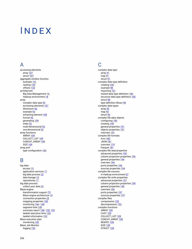
I n d e x
Aaccessing elements
array 107struct 107
aggregate window function example 131nesting 133offsets 133
architecture Big Data Management 16Hadoop environment 18
array complex data type 92accessing elements 107dimension 92example 92extracting element 108format 92generating 109index 92multi-dimensional 92one-dimensional 92
array functions ARRAY 109COLLECT_LIST 109CONCAT_ARRAY 109SIZE 109
array port type configuration 103
Bbig data
access 13application services 17big data process 22data lineage 15repositories 17
big data process collect your data 23
Blaze engine transformation support 75Blaze engine architecture 19connection properties 25mapping properties 150monitoring 146–148segment time 149summary report 148–150, 152tasklet execution time 150tasklet information 152
Blaze execution plan monitoring 145
Blaze Job Monitor logging 153
Ccomplex data type
array 91map 91struct 91
complex data type definition creating 100example 98importing 101nested data type definition 100recursive data type definition 100struct 98type definition library 98
complex data types array 92map 93struct 94
complex file data objects configuring 190creating 190general properties 191objects properties 191overview 191
complex file formats Avro 180JSON 181overview 179Parquet 181
complex file read properties advanced properties 195column projection properties 196general properties 194overview 194ports properties 194sources properties 194
complex file sources in Hadoop environment 67
complex file write properties advanced properties 197column projection properties 199general properties 196overview 196ports properties 197sources properties 197
complex files compression 192decompression 192
complex functions ARRAY 109CAST 109COLLECT_LIST 109CONCAT_ARRAY 109RESPEC 109SIZE 109STRUCT 109
206
complex functions (continued)STRUCT_AS 109
complex operator dot operator 107example 107subscript operator 107
complex port array 96creating 98map 96nested 96Read transformation 97struct 96transformations 97type configuration 96, 103Write transformation 97
component architecture clients and tools 16
configuring array port properties 103map port properties 105
struct port properties 106
connections properties 25HBase 24HDFS 24Hive 24JDBC 24
conversion hierarchical to relational 110
creating a column profile profiles 169
DData Discovery
description 14Data Integration Service grid 175data object profiles
creating a single profile 167enterprise discovery 168
data objects complex file data objects 190
data type complex data type 91nested data type 91primitive data type 91
data types complex files 179Hive 183Hive complex data types 184processing in a Hadoop environment 84support 179
dot operator extracting struct element 108
Eenterprise discovery
running in Informatica Analyst 170example
aggregate window function 131array 92complex data type definition 98complex operator 107
example (continued)dot operator 107map 93nested data type definition 100partition and order keys 128struct 94subscript operator 107windowing 135, 137
execution plan Spark engine 56
Fflat file sources
in Hadoop environment 64functions
processing in a Hadoop environment 84
Ggrid
Data Integration Service 175description 174optimization 175
HHadoop 24Hadoop connections
creating 43Hadoop environment
transformation support 74complex file sources 67flat file limitations 64flat file targets 69Hive targets 70logs 142optimization 57parameter usage 204parameters 203relational sources 67Sqoop sources restrictions 68Sqoop targets restrictions 73valid sources 63
Hadoop execution plan description, for mapping 44overview 54
Hadoop mapping run-time properties 45
hadoop utilities Sqoop 18
HBase connections MapR-DB properties 32properties 31
HDFS connections creating 42properties 29
HDFS mappings data extraction example 161description 161
hierarchical conversion generate nested struct 113generate struct 111hierarchical to hierarchical 120hierarchical to relational 120, 123
Index 207
hierarchical conversion (continued)relational to hierarchical 111, 113
hierarchical data complex files 88converting 110extracting elements 120flattening elements 123how to process 89modifying 120, 123processing 88Spark engine 88
high availability description 176
Hive target limitations 70
Hive connections creating 42properties 32
Hive engine data type processing 86function processing 86rules and guidelines 86transformation support 81Hive engine architecture 21Hive engine execution plan 57monitoring 157
Hive execution plan monitoring 145
Hive mappings description 162workflows 53
Hive pushdown connection properties 25
Hive query description, for mapping 44
Hive query plan viewing, for mapping 57viewing, for profile 172
Hive script description, for mapping 44
Hive sources with Blaze engine 65with Informatica mappings 64
Hive targets with Blaze engine 70
how to process hierarchical data 89
IInformatica Big Data Management
overview 12Informatica engine
Informatica engine execution plan 55Intelligent Streaming
description 15
JJDBC connections
properties 37Sqoop configuration 37
Llogging
mapping run on Hadoop 153Spark engine 157
logs Blaze engine 152Hadoop environment 142Hive engine 159Spark engine 157
logs URL YARN web user interface 157
Mmap
complex data type 93example 93format 93key-value pair 93
map port type configuration 105
mapping example Hive 163Twitter 164
mapping execution plans overview 54
mapping run on Hadoop logging 144monitoring 145overview 44
MDM Big Data Relationship Management description 15
Monitoring URL Blaze and Spark jobs 143
Nnative environment
high availability 176mappings 160optimization 174partitioning 175
nested data type definition example 100
nested struct generating 113
Ooptimization
compress temporary staging tables 58node labeling 61queuing 61scheduling 61truncate partitions 60
overview processing hierarchical data 88
Pparameters
Hadoop environment 203
208 Index
partitioning description 175optimization 176
processing hierarchical data overview 88
profile run on Blaze engine Overview 165
profile run on Hadoop monitoring 172
profile run on Hive Overview 165
profiles creating a column profile 169
Rrelational to hierarchical 110rules and guidelines
Spark engine 85Hive engine 86window functions 135windowing properties 130
run-time properties Hadoop mapping 45
Ssocial media mappings
description 163sources
in Hadoop environment 63Spark
execution plans 56Spark deploy mode
Hadoop connection properties 25Spark engine
data type processing 85function processing 85rules and guidelines 85transformation support 79connection properties 25hierarchical data 88monitoring 154
Spark Event Log directory Hadoop connection properties 25
Spark execution parameters Hadoop connection properties 25
Spark HDFS staging directory Hadoop connection properties 25
Sqoop configuration mapping properties 52profiling 166
Sqoop connection arguments -Dsqoop.connection.factories 40connect 40direct 40driver 40
Sqoop connectivity supported data types 185
Sqoop data types Aurora 185Greenplum 186IBM DB2 185IBM DB2 for z/OS 185Microsoft SQL Server 186Netezza 187
Sqoop data types (continued)Oracle 187Teradata 188Teradata Data Types with TDCH Sqoop Specialized Connectors 188
Sqoop mapping arguments batch 52m 51num-mappers 51split-by 51
Sqoop mappings overview 50supported engines 50
Sqoop sources in Hadoop environment 68
Sqoop targets in Hadoop environment 73
stateful computing overview 126
struct complex data type 94accessing elements 107changing data type 109changing schema 109complex data type definition 98example 94extracting element 108format 94generating 109, 111name-type pair 94schema 94
struct functions CAST 109RESPEC 109STRUCT 109STRUCT_AS 109
struct port complex data type definition 106type configuration 106
subscript operator extracting array element 108
Ttargets
flat files in Hadoop mapping 69TDCH connection factory
-Dsqoop.connection.factories 40third-party tools
hadoop cluster 18transformations
in Hadoop environment 74support on the Blaze engine 75support on the Spark engine 79
type configuration array 103map 103struct 103struct port 106
type definition library complex data type definition 98mapping 98mapplet 98nested data type definition 100
Index 209
Uutilities
hadoop cluster 18
Vvalidation environments
Hadoop mapping 45Vibe Data Stream
description 15
Wwindow functions
aggregate functions 131LAG 131LEAD 131
window functions (continued)overview 130rules and guidelines 135
windowing example 135, 137, 139overview 126properties 127
windowing properties frame 127, 133order 127, 128partition 127, 128rules and guidelines 130
workflows Hive mappings 53
YYARN web user interface
description 143
210 Index