Tricks to Creating a Resource Block Model

St John’s, Newfoundland and LabradorNovember 4, 2015

Tricks toCreating aResource Block Model

Agenda2

Domain Selection Top Cut (Grade Capping) Compositing Specific Gravity Variograms Block Size Search Ellipse Nearest Neighbour Inverse Distance Ordinary Kriging Validation Resource Classification Indicator Kriging

3

Fundamentals

GI – GOGarbage In – Garbage Out

Black Box

Domain Selection4

A domain is a spatial entity with common geological or geostatistical attributes

Domain Selection5

Most domains are selected based on geological or grades Or a combination of both

The definition of the boundaries between geological domains can be problematic due to several factors, including Defining geological domains relies on the geologist’s interpretation Sample information is limited and therefore interpreted boundaries

have a degree of uncertainty

Domains have either a “hard boundary” or “soft boundary”

Domain Selection6

Hard boundary Most common domain selection used by geologists

Based strictly on geological or geochemical constrains All material inside Quartz Porphyry unit All material contained within the “shear zone” All material on the 2.5 g/t grade shell

It is easy for the human eye to “see” the boundary and make the estimation process easier The samples are either inside the boundary or outside the boundary

Domain Selection7

Hard boundary Solids or wireframes tend to have unrealistic shapes not geologically realistic particularly with grade shells due to “snapping” to the drillhole

Domain Selection8

What do you do here?

FoldingFaulting

Domain Selection9

What do you do here?

Pinch and Swell Variable Dip

Domain Selection10

Soft boundaries A soft boundary has a gradational zone between two adjacent domains,

making it difficult to identify the exact boundary Porphyry deposits Disseminated sulphides Stringer or stockwork deposits Transition from oxide to sulphide

The estimation process using soft boundaries is complex

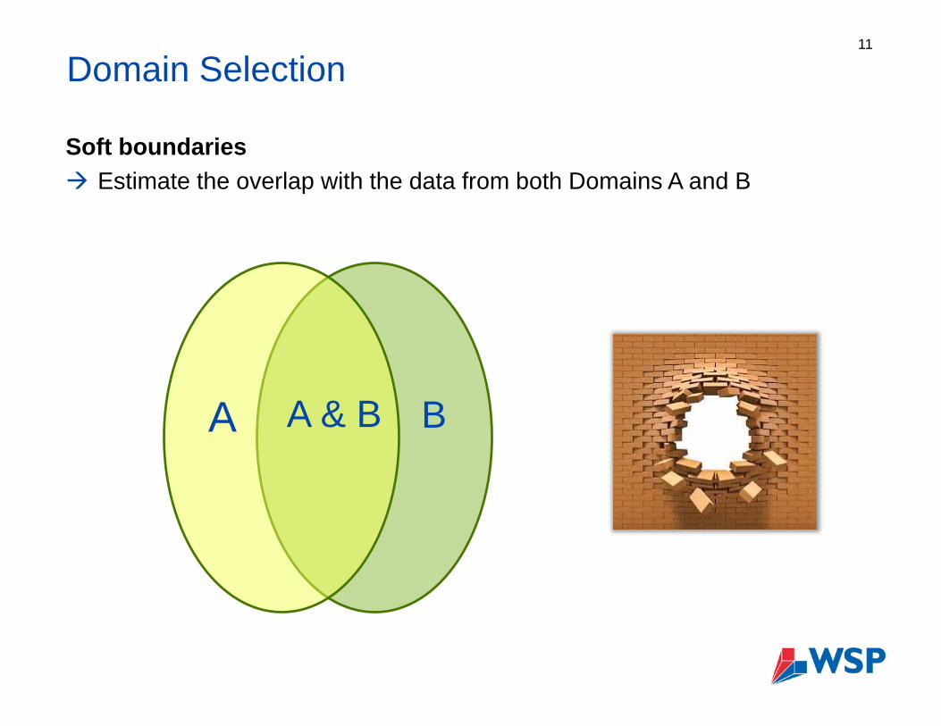
Domain Selection11

Soft boundaries Estimate the overlap with the data from both Domains A and B

A BA & B

Domain Selection12

Soft boundaries

Estimate Domain A using data from Domain A, then estimate Domain B using data from Domains A and B

Estimation of B might have a different capping strategy, variogram, and search ellipse

Estimate using data with X metres of the boundary

A B

Top Cut and Bottom Cut (Grade Capping)13

Fix all errors in the data

Do not blindly follow the advice in statistics books

Do not blindly use all data; follow local customs

Consider probability plots

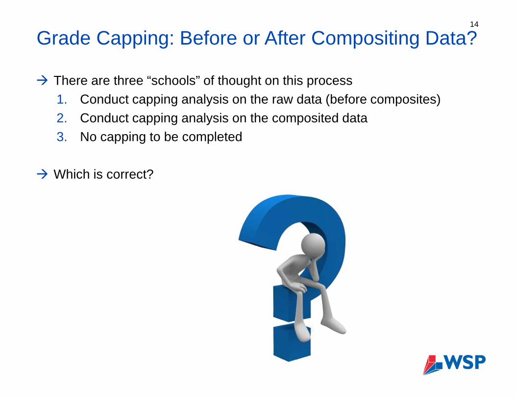
Grade Capping: Before or After Compositing Data?14

There are three “schools” of thought on this process1. Conduct capping analysis on the raw data (before composites)2. Conduct capping analysis on the composited data3. No capping to be completed

Which is correct?


Bottom cut Should be done with very large data sets that have a large population

which would be deemed as “background”

Removing bottom cut results in a the data shifting left

Probability plots Useful to identify populations and consider outlier treatment

Updated program Fits arbitrary number of populations with lines (fitted

non-parametric model) or mixture model Normal or lognormal Iterative optimization with least squares objective function Provides population adjusted values for upper tail Plots metal at risk for upper tail values

Top Cut and Bottom Cut (Grade Capping)


Some probability plots Fitted non-parametric – lines

Mixture model – curved wheredistributions overlap


Parrish Analysis (Decile Analysis) Paper in the Mining Engineering Journal

(April 1997)

Arrange the sample data into decile grouping (10%) If the top decile (90-100) has 40% or more of the metal

content, than capping may be required If the top decile (90-100) has more than twice the metal

content of the next decile (80-90), than capping may be required

If the top percentile (99-100) has more than 10% of the metal content, than capping maybe required

Before any capping, review the spatial distribution of the samples Might be a high-grade sub-domain

18


Example of a Parrish Analysis

No of Mean Minimum Maximum Metal %From To Samples Grade Grade Grade Content Metal

0 10 102 0.001 0.000 0.002 0.10 0.010 20 103 0.002 0.002 0.003 0.25 0.020 30 102 0.005 0.004 0.008 0.54 0.030 40 103 0.015 0.008 0.027 1.56 0.140 50 103 0.043 0.028 0.063 4.42 0.250 60 103 0.112 0.063 0.173 11.47 0.660 70 103 0.330 0.178 0.505 33.95 1.870 80 103 1.007 0.515 1.653 102.74 5.580 90 103 2.967 1.670 4.840 305.60 16.390 100 103 13.714 4.900 90.743 1412.52 75.4

90 91 10 5.205 4.900 5.556 52.05 2.891 92 10 5.805 5.571 6.095 58.05 3.192 93 10 6.691 6.183 7.058 66.91 3.693 94 11 7.549 7.148 7.992 83.03 4.494 95 10 8.482 7.997 8.991 84.82 4.595 96 10 9.710 9.089 10.398 97.10 5.296 97 11 12.136 10.399 13.788 133.50 7.197 98 10 15.093 13.854 16.859 150.93 8.198 99 10 19.476 17.102 22.917 194.76 10.499 100 11 44.668 23.071 90.743 491.35 26.2

%Quantile No of Mean Minumum Maximum Metal %From To Samples Grade Grade Grade Content Metal

0 10 75 0.118 0.003 0.327 7.625 0.40%10 20 73 0.558 0.334 0.760 35.360 1.86%20 30 74 0.922 0.770 1.100 59.514 3.13%30 40 73 1.237 1.100 1.380 77.712 4.09%40 50 74 1.528 1.380 1.700 96.022 5.05%50 60 73 1.919 1.700 2.140 114.261 6.01%60 70 74 2.483 2.150 2.830 144.685 7.61%70 80 73 3.363 2.830 3.940 209.012 10.99%80 90 74 5.115 3.956 6.530 305.072 16.04%90 100 73 19.791 6.757 162.800 853.086 44.84%

90 91 7 7.073 6.757 7.420 32.419 1.70%91 92 7 7.849 7.500 8.230 44.443 2.34%92 93 8 8.802 8.275 9.330 50.064 2.63%93 94 7 9.953 9.529 10.400 50.212 2.64%94 95 7 11.324 10.580 11.950 57.287 3.01%95 96 8 13.179 11.967 14.190 70.547 3.71%96 97 7 16.229 14.695 16.890 74.026 3.89%97 98 7 18.478 17.200 20.300 79.556 4.18%98 99 8 26.650 21.040 32.830 131.185 6.90%99 100 7 79.906 38.890 162.800 263.348 13.84%

%Quantile

Sample Compositing20

Procedure of combining adjacent values into longer down-hole intervals

These are usually weighted by length, and possibly by specific gravity and core recovery


Compositing leads to one of the following results Orebody intersections Lithological or metallurgical composites Regular length composites Bench composites or section composites High-grade composites Minimum length and grade composites

Each of these types of composite are produced for different purposes and in different situations

Regular length or bench composites are common in geostatistical analysis Geostatistical software assumes the data represent the same volume The length should be small enough to permit resolution of the final simulated

grid spacing The length shall respect domain contacts


Factors to consider Mean sample length

Median sample length

Potential block size

Potential mining width or height

Composites should not be shorter than the median sample length

Composites should be 1/3 to 1/2 the block size

Composites should be 1/3 to 1/2 the mining width

Most geostatisticians like longer composites (regardless of the geology)


Compositing procedure Top of hole Top of interval Bottom of interval Bench

Watch for “tails” A small interval remaining after the composites are completed Tend to be at the end of the interval

How to deal with tails Ignore Include “Backstitch”

Specific Gravity24

The ratio between the density of a material and the density of water

Specific Gravity25

In the metric system, specific gravity (SG) and density are the same value

In the imperial system, SG and density are different values

Not to be confused with tonnage factor

Could be one of the more important numbersin a resource estimation

Global SG

Linear equation

Polynomial equation

There is a temperature correction The SG of water is 1 at 4°C

Specific Gravity26

Polynomial equation based on measured values

Specific Gravity27

Why is SG so important in a resource model? Assume a block model with 10 x 10 x 10 m blocks

Each block has a volume of 1,000 m3

Tonnage of the block is volume x SG

SG = 2.75, then the tonnage is 2,750 t

SG = 2.76, then the tonnage is 2,760 t

Just added 10 tonnes per block by changing the SG by 0.01

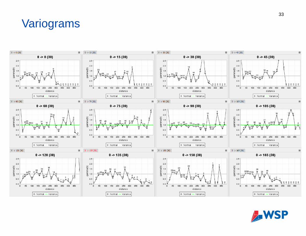
Variograms28

The empirical variogram provides a description of how the data is related (correlated) with distance

Variograms29

Components to make a variogram Azimuth: the horizontal direction the variogram searches

Plunge: the vertical direction the variogram searches

Lag: the distance between samples

Maximum distance: how far out to search

Spread: the cone angle to search

Spread limit: the maximum radius of the spread

Search Line

Spread

Spread Limit

Variograms

Components of a variogram Nugget: no spatial correlation from a the geological microstructures and

measurement errors

Sill: is the variance

Range: is the distance at which the variogram reaches the sill

30

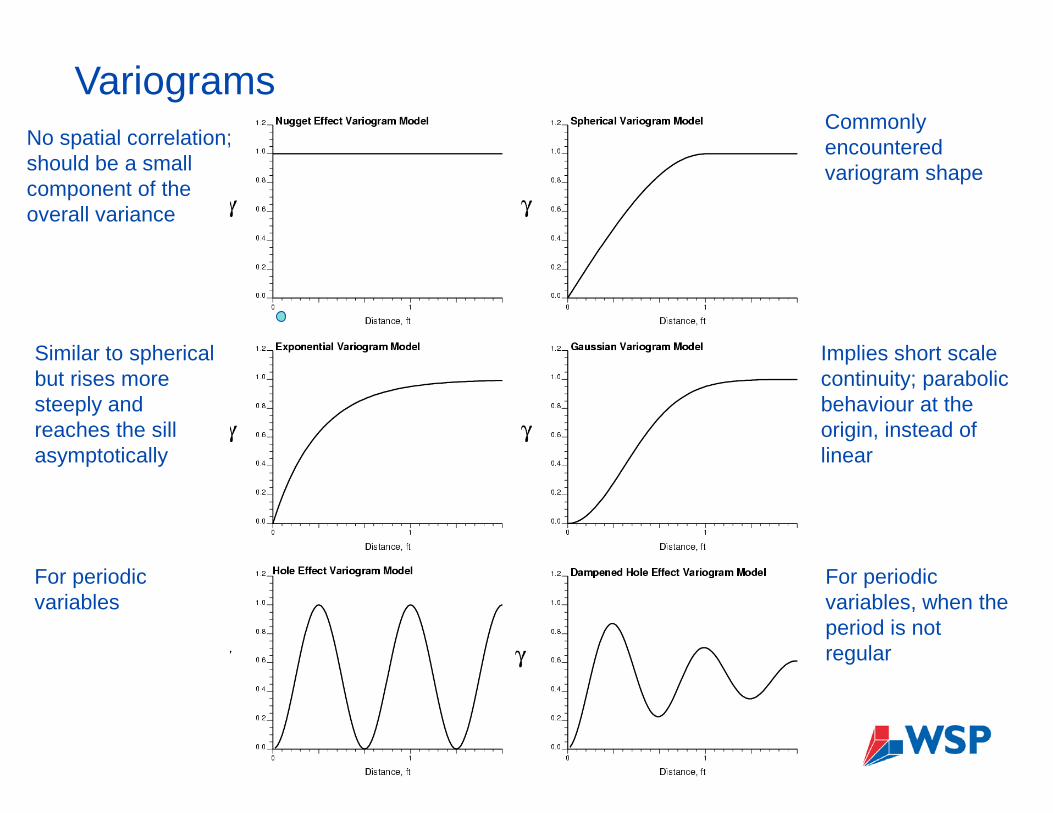
VariogramsNo spatial correlation;should be a small component of the overall variance

Commonly encounteredvariogram shape

Similar to spherical but rises more steeply and reaches the sill asymptotically

Implies short scale continuity; parabolic behaviour at the origin, instead of linear

For periodic variables

For periodic variables, when the period is not regular

Variograms

To improve the variogram Increase lag distance

Change rotation direction

Open or narrow spread

Allow overlap

Hide “pairs” less than 50, 100, 1000

32

0

0.2

0.4

0.6

0.8

1

1.2

2 4 6 8 10 12 14 16 18 20 22 24 26 28 30

Variance

0

0.2

0.4

0.6

0.8

1

1.2

1.4

1.6

2 4 6 8 10 12 14 16 18 20 22 24 26 28 30

Variance

Variograms33

Variograms34

Variograms35

Ensure a positive definite model by Picking a single (lowest) isotropic nugget effect Choosing the same number of variogram structures for all directions

based on most complex direction Ensuring that the same sill parameter is used for all variogram

structures in all directions Allowing a different range parameter in each direction Modeling a zonal anisotropy by setting a very large range parameter in

one or more of the principal directions Rotation direction of the variogram may not match geology

The responsibility is yours, but most software helps

Variogram modeling is one of the most important steps in the geostatistical study, however, do not spend days on it

Variograms

Block Size37

Block Size Selection

Some factors to consider The sample interval of the data; there's not a lot of point in being smaller than

that What is the scale of your problem? If this is part of an exploration exercise and

the model is really large, then you can safely and justifiably lose temporal resolution

How much time have you got? Small samples means more compute time, more statistics, more fiddling with details

1/3 to 1/2 sample spacing is typical Smallest mining unit Blocks do not have to be cubes (2 x 2 x 2) or (5 x 5 x 2) Sub-block or sub-cell Be careful of the sub-block routine

Smaller blocks does not mean more accuracy A block grade is the average of the estimation at the discretization points

38

Search Ellipse39

Search Ellipse

Creation of search ellipse The dimension of the ellipse should be generated from variogram model Based on the ratio of the Major / Semi-major / Minor Axis Rotation angle should mimic the geology

40

Search Ellipse

Search ellipse Different search ellipse rotations would be required as the mineralization

geometry changes (Dynamic Anisotropy)

41

Nearest Neighbour42

Nearest Neighbour

Provides the best global estimate Should not be used in a resource statement (if possible)

Estimates the grade of the block from the closest data point Uses a single sample point Does not take into account the distance from the sample Does not take into account the relative direction of the sample

Inverse Distance44

Inverse Distance

Used for early estimations and validation Can use several samples in the

estimation The distance of the sample is the

weighting factor Relative direction is not accounted for

in the estimation (Surpac might be different in this case)

The variance is not accounted for in the estimation

A power of 2 is the most common Power of 3 is acceptable

Increasing power makes the estimate “like” a nearest neighbour estimate

𝑊𝑊 𝑑𝑑 =1𝑑𝑑𝑝𝑝

Kriging46

Ordinary Kriging

Context The goal is to compute a best estimate at an un-sampled location

Considers the data as differences from their mean values

Statistical inference and a decision of stationarity provides the required information

Weights could be positive or negative, depending on relationship between unsampled location and data

Considering quadratic or higher order terms increases inference and does not lead to improved estimates

Co-variances are calculated from the variogram model

Ordinary Kriging48

Kriging will be similar to other estimation methods

If the data locations are fairly dense and uniformly distributed throughout the study area, fairly good estimates regardless will be obtained, regardless of interpolation algorithm

If the data locations fall in a few clusters with large gaps in between, unreliable estimates will be obtained, regardless of interpolation algorithm

Almost all interpolation algorithms will underestimate the highs and overestimate the lows; this is inherent to averaging and if an interpolation algorithm did not average, it would not consider it reasonable

Ordinary Kriging49

Some advantages of kriging

Helps to compensate for the effects of data clustering, assigning individual points within a cluster less weight than isolated data points (or, treating clusters more like single points)

Gives estimate of estimation error (kriging variance), along with estimate of the variable, Z, itself (but error map is basically a scaled version of a map of distance to nearest data point, so not that unique)

Availability of estimation error provides basis for stochastic simulation of possible realizations of Z(u)

Ordinary Kriging

Parameters to adjust during estimation runs Minimum number of samples Too low will use only a single sample Too high might not find enough data points to complete the estimate

Maximum number of samples Too low Too high results in an over-smoothed estimate

Maximum number per drillhole Too low results in a single sample per hole and not enough samples to

satisfy the minimum number of samples criteria Too high results in the entire holes being used in the estimate

50

Ordinary Kriging51

KE=(BV-KV)/BVA number between 0 and 1

Ordinary Kriging52

Ordinary KrigingEstimation strategies 3 or 4 estimation passes On each estimation pass the search ellipse is increased and the min/max criteria is adjusted There is not perfect fit

Pass 1- Smallest search ellipse (50% to 65% of variogram range)- Min samples 4 to 5- Max samples 15 to 20- Max / hole 2 or 3

Pass 2- Search ellipse (70% to 85% of variogram range)- Min samples 3 to 5- Max samples 15 to 20- Max / hole 2 or 3

Pass 3- Full search ellipse (100% of variogram range)- Min samples 2 to 5- Max samples 15 to 20- Max / hole 2 or 3

Pass 4- Large search ellipse (125% to 200% of variogram range)- Min samples 2 or 3- Max samples 15 to 20- Max / hole 2 or 3

53

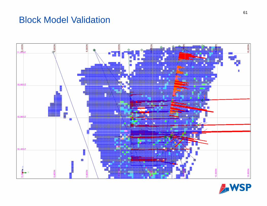
Block Model Validation54

WHY CHECK?

Block Model Validation

Resource model integrity

Field procedures Starting from scratch”; checking related to

- sampling- collar locations- topographic- down-the-hole surveys- drilling methods- sample collection and preparation- assaying, and sample quality control- quality assurance program

Data handling and processing


Resource model validation

Geological model validation Cross-check between solid and block model proportions

Statistical validation Statistical data (mean and variances) between dataset and block model Swath plots – grade trends analysis between declustered composite

grades and block model grades Contact analysis – grade behaviour near contact zones

Graphical validation Grade-tonnage curve Cross-sectional view, looking for spilling grades


Resource model validation Statistical validation – comparison between dataset and block model


Resource Model Validation Statistical validation – swath plots


Resource model validation Statistical validation – contact analysis

Resource Classification63

Historical Approaches

Expert assessment of geological continuity Distance from a sample(s) Sample density in the vicinity of a block Geometric configuration of data available to estimate a block Kriging variance or relative kriging variance

Geometric Measures

Geometric measures such as drillhole spacing, drillhole density, and closeness to the nearest drillhole are direct measures of the amount of data available

They are related

dLL 10000

221 =

+

21

10000LL

d⋅

=

and

222

21 )2( rLL =+

4

22

21 LLr +

=

Calculating Geometric Measures

Calculate the density of data per unit volume

Choice of thresholds depend on Industry-standard practice in the country and geologic province Experience from similar deposit types Calibration with uncertainty quantified by geostatistical calculations Expert judgement of the Competent or Qualified Person

210000

srnd

⋅⋅

=π d

L 10000=

Uncertainty

Geometric methods for classification are understandable, but do not give an actual measure of uncertainty or risk

Professionals in ore reserve estimation increasingly want to quantify the uncertainty / risk in their estimates

Classification of Resources and Reserves

Three aspects of probabilistic classification1. Volume2. Measure of “+/-” uncertainty3. Probability to be within the “+/-” measure of uncertainty

Format for uncertainty reporting is clear and understandable, e.g.: Monthly production volumes where the true grade will be within 15% of

the predicted grade 90% of the time are defined as measured Quarterly production volumes where the true grade will be within 15% of

the predicted grade 90% of the time are defined as indicated

Drillhole density and other geometric measures are understandable, but do not really tell us the uncertainty or risk associated with a prediction

There are no established rules or guidelines to decide on these three parameters; that remains in the hands of the Qualified Person

Example of Probabilistic Classification Note the limited number of

drillholes

A reference histogram and variogram are used

The probability to be within +/-50% of the estimated grade could be used for classification

More Drilling and a Change in Modeling More drillholes

(190 vs. 21 before)

Different decision of stationarity

New calculation of probabilities

The probability to be in interval has mostly increased, but 16% of the probabilities are lower!

Indicator Kriging71

Indicator Kriging

A variogram is needed for each threshold More difficult inference problem, however, there is great flexibility

Too few – insufficient resolution of the estimated distributions

Too many – insufficient data in the neighbourhood for reliable estimates

Conventional practice – consider 7 to 12 thresholds considering Regular spaced (probability) quantiles of the global distribution, say the

nine deciles (z0.1, z0.2, … z0.9) plus a high value z0.95

Resolution where needed – may need less in the low grades Consider the economic cutoff Consider inflection points on the probability plot

Standardize all points and models to a unit variance p(1-p)

Model the variograms with smoothly changing parameters for a consistent description Common origin imparts

consistency Reduced order relations in

IK/SIS Allows straightforward

interpolation of models for new cutoffs

Indicator Kriging

Indicator Variogram Models

In this case Nugget is larger for the first and last cutoff

Medium range exponential model with consistently increasing range, contribution, and anisotropy

Long range spherical model with decreasing range, decreasing contribution, and increasing anisotropy

Conclusion

Tricks to Creating a Resource Block Model

Documents

Transcript of Tricks to Creating a Resource Block Model