Georgia State University Georgia State University

ScholarWorks @ Georgia State University ScholarWorks @ Georgia State University

Physics and Astronomy Theses Department of Physics and Astronomy

Fall 12-1-2013

Transforming High School Physics With Modeling And Transforming High School Physics With Modeling And

Computation Computation

John M. Aiken Georgia State University

Follow this and additional works at: https://scholarworks.gsu.edu/phy_astr_theses

Recommended Citation Recommended Citation Aiken, John M., "Transforming High School Physics With Modeling And Computation." Thesis, Georgia State University, 2013. https://scholarworks.gsu.edu/phy_astr_theses/18

This Thesis is brought to you for free and open access by the Department of Physics and Astronomy at ScholarWorks @ Georgia State University. It has been accepted for inclusion in Physics and Astronomy Theses by an authorized administrator of ScholarWorks @ Georgia State University. For more information, please contact scholarworks@gsu.edu.

TRANSFORMING HIGH SCHOOL PHYSICS WITH MODELING AND COMPUTATION

by

JOHN M. AIKEN

Under the Direction of Brian D. Thoms

ABSTRACT

The Engage to Excel (PCAST) report, the National Research Council's Framework for K-12 Science

Education, and the Next Generation Science Standards all call for transforming the physics classroom

into an environment that teaches students real scientific practices. This work describes the early stages

of one such attempt to transform a high school physics classroom. Specifically, a series of model-

building and computational modeling exercises were piloted in a ninth grade Physics First classroom.

Student use of computation was assessed using a proctored programming assignment, where the stu-

dents produced and discussed a computational model of a baseball in motion via a high-level program-

ming environment (VPython). Student views on computation and its link to mechanics was assessed

with a written essay and a series of think-aloud interviews. This pilot study shows computation's ability

for connecting scientific practice to the high school science classroom.

INDEX WORDS: Computational Modeling, Physics, Education

TRANSFORMING HIGH SCHOOL PHYSICS WITH MODELING AND COMPUTATION

by

JOHN M. AIKEN

A Thesis Submitted in Partial Fulfillment of the Requirements for the Degree of

Masters of Science

in the College of Arts and Sciences

Georgia State University

2013

Copyright by

John Mark Aiken

2013

TRANSFORMING HIGH SCHOOL PHYSICS WITH MODELING AND COMPUTATION

by

JOHN M. AIKEN

Committee Chair: Brian D. Thoms

Committee: Marcos D. Caballero

Michael F. Schatz

Raj Sunderraman

Electronic Version Approved:

Office of Graduate Studies

College of Arts and Sciences

Georgia State University

December 2013

iv

ACKNOWLEDGEMENTS

I would like to acknowledge everyone who has participated in providing me with a transforma-

tive experience in my Masters program. Mike Schatz and Brian Thoms have fulfilled complimentary roles

as advisers. Danny Caballero and Shih-Yin Lin have given me valuable research advice. I’d also like to

acknowledge Scott Douglas, whose aid in coding and quantifying data has been enlightening, and Chasti-

ty Aiken, my wife, whose own expertise in research has been as valuable as her personal advice and

support.

vi

TABLE OF CONTENTS

ACKNOWLEDGEMENTS .......................................................................................................... v

LIST OF TABLES ................................................................................................................... viii

LIST OF FIGURES ..................................................................................................................... x

1 INTRODUCTION AND BACKGROUND .................................................................................. 1

1.1 Transforming High School Physics for the 21st Century ..............................................1

1.2 Building on a Research Base: Modeling and Computation ..........................................5

1.3 Modeling Instruction for High School Physics ............................................................7

1.3.1 What Is a Scientific Model? ..................................................................................7

1.3.2 Modeling Cycle ....................................................................................................8

1.3.3 An Example of a Modeling Instruction Model: Constant Velocity ......................... 10

1.3.4 Effectiveness of Modeling Instruction ................................................................. 12

1.3.5 Modeling Instruction's Goals for Teachers .......................................................... 15

1.4 Prior Use of Computation in 20th Century Science Classes ....................................... 16

1.5 Incorporating Computation into High School Physics ............................................... 19

1.6 Research Questions ................................................................................................ 22

2 ASSESSING STUDENT USE OF COMPUTATION IN A HIGH SCHOOL PHYSICS CLASS ............... 23

2.1 Introduction ........................................................................................................... 23

2.2 Proctored assignment ............................................................................................ 26

2.3 Essay questions ...................................................................................................... 30

vii

2.4 High School Student Interviews .............................................................................. 33

3 CONCLUSIONS .................................................................................................................. 35

3.1 Discussion .............................................................................................................. 35

3.2 Looking Back .......................................................................................................... 37

3.3 Looking Forward .................................................................................................... 37

REFERENCES ............................................................................ Error! Bookmark not defined.40

APPENDICES ........................................................................................................................ 48

A.1 Reasons for Choosing Python as a Learning Language .............................................. 48

A.2 Computational Activities Designed and Used by John Burk ...................................... 48

A.2.1 Introduction to Computational Modeling ........................................................... 50

A.2.2 WebAssign Constant Velocity Assignment .......................................................... 52

A.3 Student Technology Survey Results ......................................................................... 57

A.4 Proctored Assignment ............................................................................................ 59

A.4.1 Code That was given to students at the beginning of the assessment .................. 59

A.4.2 An example of successful code ........................................................................... 61

viii

LIST OF TABLES

Table 1 : Skills sought after by top employers [2]. ...............................................................................3

Table 2: Comparison of students' activities with those of a professional physicist[4]. ...........................4

Table 3: NRC Framework for K-12 Science Education[3]. ......................................................................5

Table 4: Instructional goals of the constant velocity model unit. ........................................................ 10

Table 5 : Constant velocity model sequence. ..................................................................................... 12

Table 6 : Results from two Physics First and Modeling Instruction studies. L. Liang's study had a total of

301 participating students in grades 9-12 [30]. M. O'Brien's study had a total of 321 students

participate[33]. M. O'Brien did not report standard deviation and reported average scores not

percentages (represented in parantheses). ....................................................................................... 14

Table 7 : Students were asked the question "Do you know anything about programming a

computer?". If they responded yes they were asked to explain their experiences (N=36). One student

who answered "yes" to the initial question responded in the follow up question explaining their

experience with " Like downloading software from a CD". This was marked as "None" for answer

purposes .......................................................................................................................................... 21

Table 8: Codes validated in previous work used for the proctored assignment [59]. Codes marked with

asterisks(*) were not applicable to the proctored assignment. GT students who were tasked with

modeling the motion of planets became confused when trying to select the appropriate exponent of

the interaction constant [59]. This issue does not arise when modeling projectile motion and thus IC5

was not needed. In orbital motion, an explicit separation vector is required due to the nature of

motion (i.e., where is the separation vector and not necessarily zero), GT students attempted to raise

this to a power (when in fact it is the magnitude of the difference that should be raised not the vector)

[59]. In projectile motion the separation vector is always zero therefore there is never a need to

interact with it (this is the excluded FC3). Due to the simplicity of the forces involved in the proctored

ix

assignment students didn't have any other force direction confusion (the only force direction would

be the direction of gravity) thus FC5 was inapplicable. Using Euler-Cromer integration to represent

Newton's 2nd law programmatically, students modeling orbital motion often had difficulties

differentiating between when to use a scalar or a vector [59]. Since the acceleration is one

dimensional in projectile motion SL3 was not needed. SL4 was in regards to momentum updates and

the proctored assignment does not consider momentum in its calculations (students were told force is

not the more general ) [59]. In projectile motion, the "massive particle" is the Earth. Generally,

Newton's theory of gravitation will work for this situation. However this can be reduced to for

projectile motion and this is done for the proctored assignment removing the need for O1. .............. 27

Table 9:Student views with examples. Highlighted portions (in grey) indicate sections coded as

applying to the associated view. Examples might include multiple views but this in not included in

these examples. ............................................................................................................................... 33

Table 10 : This table has been reproduced from [69]. ........................................................................ 48

x

LIST OF FIGURES

Figure 1: A motion diagram of a car moving at constant velocity. This image is used in a Modeling

Instruction worksheet [24]. ............................................................................................................. 10

Figure 2: Students are asked to move in front of a motion detector to reproduce the position versus

time and motion map represented in this image. .............................................................................. 11

Figure 3 : Student FCI mean scores. Modified from Ref. 9. Jackson did not report error or significance

in her study. .................................................................................................................................... 15

Figure 4 : Example VPython screenshot of the animation of a baseball in flight. This animation would

appear as a real time update of the integration calculation on a computer. Note the motion map and

force vector arrows. These are sized by the magnitude of the vector they represent. ........................ 18

Figure 5: Students who displayed Force-casual and Iterative views were more likely to be successful on

the proctored assignment (N=29). The bars represent a total proportion of the class (that is out of

100%). The percentages in this graph are different than the proctored assignment because the

number of students who responded to the essays is slightly less (proctored assignment N=32). ......... 31

1

1 INTRODUCTION AND BACKGROUND

1.1 Transforming High School Physics for the 21st Century

The high school physics classroom of the 21st century is failing at preparing students for under-

graduate studies and the work place [1-3]. This is because, in part, the average classroom does not focus

on teaching scientific practices (like computation, modeling, communicating, etc.) and instead stresses

content acquisition and "fact learning" [3]. When surveyed, over 400 employers report that high school

students possess none of the skills they expect new employees to possess. Employers rated four skills as

most important: work ethic, oral and written communications, the ability to collaborate, and critical

thinking (see Table 1 for the full list); when surveyed, high school graduates are inadequate in all of the-

se skills [2]. Further, the Engage to Excel report to the President of the United States (PCAST report) es-

timates that there will be approximately three million new Science, Technology, Engineering, and Math-

ematics (STEM) jobs opening in the next decade [1]. The PCAST report also projects that the current

production of STEM professionals will only fill about two thirds of the available jobs. This failure to pre-

pare an adequate number of STEM majors for STEM jobs is, in part, because only ~40% of declared

STEM majors finish their STEM undergraduate programs [1]. When surveyed, high-achieving students

most often cite "uninspiring introductory courses" as their reason for dropping out [1]. The PCAST report

recommends five ways to keep and attract people to STEM degree programs:

(1) Catalyze widespread adoption of empirically validated teaching practices;

(2) Advocate and provide support for replacing standard laboratory courses with

discovery based research courses;

(3) Launch a national experiment in postsecondary mathematics education to ad-

dress the mathematics preparation gap;

2

(4) Encourage partnerships among stakeholders to diversify pathways to STEM

careers; and

(5) Create a Presidential Council on STEM Education with leadership from the ac-

ademic and business communities to provide strategic leadership for trans-

formative and sustainable change in STEM undergraduate education.

Of the five paths to achieving the PCAST report's goal, high school physics courses are already

well equipped to tackle the first two. The Physics Education Research community has a long history of

informing the pedagogy and curricula of high school physics classrooms. These instructional innovations

include research-validated curriculum design, lessons learned from cognitive science, new tools for stu-

dents to use, and systematic measurements of affect, attitude, and efficacy [4-10]. But what does the

anatomy of science education reform look like? And how will it be specifically delivered to science

teachers?

The National Research Council's Framework for K-12 Science Education declares that the most

effective way to teach science is to have students learning the practices of a professional scientist [3].

The framework highlights three major dimensions in which science education should be better aligned

with science practice:

(1) Scientific and engineering practices

(2) Crosscutting concepts that unify the study of science and engineering

through their common application across fields

(3) Core ideas in four disciplinary areas: physical sciences; life sciences; earth

and space sciences; and engineering, technology, and applications of science

3

Scientific practices include critical thinking by "asking questions and defining problems", building com-

munication skills by "constructing explanations and designing solutions", and using computation and

model building to solve real world problems [3]. The framework's emphasis on making science class

more like professional science practice motivated much of the research and classroom implementation

found in this thesis. This work focuses chiefly on the introduction of two scientific practices into the high

school physics classroom: computation and model building.

Table 1 : Skills sought after by top employers [2].

Basic Knowledge/Skills Applied Skills

English Language (spoken)

Reading Comprehension (in English)

Writing in English (grammar, spelling, etc.)

Mathematics

Science

Government/Economics

Humanities/Arts

Foreign Languages

History/Geography

Critical Thinking/Problem Solving

Oral Communications

Written Communications

Teamwork/Collaboration

Diversity

Information Technology Application

Leadership

Creativity/Innovation

Lifelong Learning/Self Direction

Professionalism/Work Ethic

Ethics/Social Responsibility

How, then, do professional scientists practice science? That is, can real scientific practice (specif-

ically computation and model building) be characterized in a consistent way? And how do these practic-

es compare to what students do in an introductory physics course? In his seminal work with the Mary-

land University Project in Physics and Educational Technology (M.U.P.P.E.T.), Edward Redish reported

that introductory college physics courses "introduce[d] students to the basic content of physics, [but

they] provide[d] almost no activities that illustrate how research is done," [4]. Redish's comparison be-

tween the practices of students and the practices of a professional scientist show a stark reality; science

class does not resemble professional science (see Table 2). In class, students are given laws and rules

from on high, and have personal ownership of them; scientists tweak and play with models in their at-

tempts to describe physical phenomena, demonstrating familiarity with and ownership of the models.

4

Students attempt to solve analytically tractable problems; scientists most often address problems which

have no analytic solution, and so they use numerical methods. Thus, Redish claims students are not us-

ing tools like computers to solve meaningful problems in the same way that scientists do.

Table 2: Comparison of students' activities with those of a professional physicist [4].

Students: Professional Scientists:

Solve narrow, pre-defined problems of no personal

interest

Solve broad, open ended and often self discovered

problems

Work with laws presented by experts. Do not "dis-

cover" them on their own or learn why we believe

them. Do not see them as hypotheses for testing.

Work with models to be tested and modified.

Know that "laws" are constructs.

Use analytic tools to get "exact" answers to inexact

models.

Use analytic and numerical tools to get approxi-

mate answers to inexact models.

Rarely use a computer. Uses computers often.

Students also know that the science classroom does not resemble professional science. When

surveyed about physics’ “real-world connections” using the Colorado Learning Attitudes about Science

Survey (CLASS), students demonstrate a significant difference in their views and the views of profession-

al physicists [5]. The CLASS aims to measure "student's beliefs about physics and learning physics" [5].

Consisting of 36 items concerning topics likes problem solving (confidence, sophistication, etc.), real-

world connections, and personal interest, the CLASS has shown that overall, physics instruction has a

negative impact on student's attitudes towards physics. Furthermore, physics instruction has a more

significant impact on women's attitudes towards physics. Some instructional reformers have empha-

sized to need to highlight "real-world connections" to create positive attitudes and increased conceptual

understanding, but what does this look like in the classroom [1, 3]?

The Investigative Science Learning Environment (ISLE) labs exposed students in an introductory

physics course to an environment that encouraged scientific thinking and practices [6]. ISLE provides

instructors with course structure guidelines, lab activities, and rubrics. ISLE focuses on helping students

develop scientific reasoning. Students in this course respond positively. Students participating in an in-

troductory college physics lab designed to teach practices valuable in the workplace exhibited expert-

Formatted Table

5

like sense making and experimental design behavior [6]. These results could not be replicated in a tradi-

tional laboratory, even when the laboratory curriculum was augmented with conceptual and reflection

questions.

1.2 Building on a Research Base: Modeling and Computation

Changing how physics is taught,such as ISLE, can lead students to become more scientist-like in

their thinking. Such changes give students the opportunity to practice using new tools to solve problems

(like computation and modeling), and expand their ability to communicate and work with others. This

work attempts to make high school science more like real science in two ways:

1. Students will build predictive models of physical phenomena that they can observe in

their world.

2. Students will actively engage in building computational simulations and modeling to

solve these problems.

This work focuses on the NRC framework's Science and Engineering practices dimension [3].

While there are eight total scientific practices emphasized by the NRC, two of these practices stand out:

developing and using models, and using computational thinking (see Table 3). It is important to align our

goals with the NRC framework for two reasons: (1) Education transformation should be focused on re-

search-validated practices [1], (2) Next Generation Science Standards (NGSS) are based on the NRC

framework [7].

Table 3: NRC Framework for K-12 Science Education [3].

The Three Dimensions of the Framework

Scientific and Engineering Practices Asking questions (for science) and defining problems (for

engineering)

Developing and using models

Planning and carrying out investigations

Analyzing and interpreting data

Using mathematics and computational thinking

Constructing explanations (for science) and designing solu-

Formatted Table

6

tions (for engineering)

Engaging in argument from evidence

Obtaining, evaluating, and communicating information

Crosscutting Concepts Patterns

Cause and effect: Mechanism and explanation

Scale, proportion, and quantity

Systems and system models

Energy and matter: Flows, cycles, and conservation

Structure and function

Stability and change

Disciplinary Core Ideas Physical Sciences

PS1: Matter and its interactions

PS2: Motion and stability: Forces and interactions

PS3: Energy

PS4: Waves and their applications in technologies for in-

formation transfer

Life Sciences

LS1: From molecules to organisms: Structures and process-

es

LS2: Ecosystems: Interactions, energy, and dynamics

LS3: Heredity: Inheritance and variation of traits

LS4: Biological evolution: Unity and diversity

Earth and Space Sciences

ESS1: Earth’s place in the universe

ESS2: Earth’s systems

ESS3: Earth and human activity

Engineering, Technology, and Applications of Science

ETS1: Engineering design

ETS2: Links among engineering, technology, science, and

society

Computation and modeling were singled out from among all the NRC practices because they

feature prominently in the Modeling Instruction (MI) curriculum. The MI curriculum has a long history of

research supporting its success at core content acquisition through teaching procedural modeling build-

ing to students [8-10],. The MI curriculum emphasizes model building, experimentation, and using scien-

tific practices in the classroom. MI will be described thoroughly in Section 1.3. Computation has a long

history of education research both in and out of physics[11-14]. In physics education research specifical-

ly, computation is often taught with the Python programming language augmented with the Visual

7

module (the language/module pair is colloquially called "VPython"). VPython gives students access to

animations, graphs, and a host of other scientific tools [15]. In addition, another Python module named

PhysUtil provides specific tools that link VPython to the MI curriculum [16], and is used extensively in

computational work described here. VPython will be described in Section 1.4.

1.3 Modeling Instruction for High School Physics

Traditional physics education consists of lectures, disconnected labs, and little interaction be-

tween students and their peers or with faculty [17]. The Modeling Instruction (MI) curriculum was cre-

ated to change high school physics class into a place where students explored physical phenomena with

experimentation and systematic analysis [8]. MI aims to help students achieve four specific goals [18].

These goals are:

1. make sense of a physical experience,

2. understand scientific claims,

3. articulate coherent opinions of their own and defend them with cogent arguments, and

4. evaluate evidence in support of justified belief.

To facilitate these goals in the classroom, students are tasked with testing "scientific models" that de-

scribe physical phenomena. The modeling process is foreign to the traditional classroom setting [8].

Therefore, teachers were trained in the MI curriculum in workshops. Activities were created to explore

each model described within the MI curriculum; these activities are available on the Modeling Instruc-

tion website free of charge [19].

1.3.1 What Is a Scientific Model?

There is no unique definition of the word "model" in the scientific literature [10]. The authors of

MI agree that a "model" has a "well defined scope" [10]. When queried, scientists define models as gen-

eral frameworks that govern specific behavior found in nature, but not as rigorously as a theory [10].

8

The MI authors define a scientific model as a "conceptual system mapped, within the context of a specif-

ic theory, onto a specific pattern in the structure and/or behavior of a set of physical systems so as to

reliably represent the pattern in question and serve specific functions in its regard" [10]. As a practical

example, the "conceptual system" might be a physical concept like "constant velocity", where the be-

havior is dictated by a stationary or moving object that does not exhibit any acceleration. This model can

be represented with equations (e.g., vt

r∆=∆

rr

), graphs, and diagrams; a plurality of representations is a

general feature of models. A constant velocity model serves a very specific function; it cannot explain,

for example, the motion of an object experiencing a non-zero net force, so another model is required to

explain this behavior.

Scientists build and use models in a similar way, with similar limitations. The Hodgkin-Huxley

model for action potentials in neurons describes the biophysical behavior of cell membranes. This model

was a very good model, earning Hodgkin and Huxley the Nobel Prize in "Physiology or Medicine" in 1963

[20], but it made assumptions that ended up failing under experimental investigation and thus has been

updated and expanded [21]. Likewise, plate tectonics, the model that describes how the Earth's surface

moves, originally did not include a motivation for this movement. It wasn't until the 1960s that mantle

convection provided evidence for what motivated plate movement [22]. In both cases, scientists started

with a model, attempted to verify its explanation via experiment or observation, and changed the model

or created a new one when the current model did not accurately explain the observed phenomena. The

modeling process in MI is built to align with professional research. This process is called the "modeling

cycle" [9].

1.3.2 Modeling Cycle

The "modeling cycle" is broken into two major steps: (1) the "Model Development" stage, and

(2) the "Model Deployment" stage. Students begin the Model Development stage by learning about a

9

new model via a pre-lab demonstration and discussion. They then participate in a "paradigm experi-

ment", exploring a particular physical phenomenon with experiment and observation in small groups.

This is followed with a post-lab discussion. Students present their results to the class and participate in a

discussion of the failings or successes of each group's experiment. The experiment/observation process

of the Model Development stage is followed by the Model Deployment stage. In this stage, the students

are tasked with completing worksheets that ask students to further develop concepts by interacting

with various representations of the model (e.g., graphs, equations, diagrams (see Figure 1), etc.). These

worksheets are usually completed in small groups [9]. Students also are given quizzes that ask concep-

tual and quantitative questions. The final assessment in the Model Deployment stage is a lab practicum

and a test. The lab practicum asks the students to design an experiment that uses the model they have

been studying to solve a real world problem. This real-world problem often asks students to extend their

knowledge. For instance, a common lab practicum for the constant velocity model has students predict-

ing the position where two constant-velocity carts collide, assuming they travel at different speeds [19,

23]. This practicum has students practicing data gathering, using their models to predict future behavior,

and exposes them to the idea of momentum transfer, which cannot be explained with a model describ-

ing only constant velocity. Before being introduced to a new model, students are given a summative as-

sessment exam that assesses their problem solving. MI is supported by free materials hosted on the

American Modeling Teachers Association (AMTA) website, as well summer modeling workshops

[8,18,19]. These materials are comprehensive, and include learning goals, activities, and experiments.

An example of these materials is detailed below.

Figure 1: A motion diagram of a car moving at constant velocity.

1.3.3 An Example of a Modeling Instruction Model

The recently updated (2010) constant velocity unit introduces students

models, and to their experimental tools

goals of the unit aimed at the instructor.

mathematical vernacular of kinematics, and

sign. A full description of these goals can be found in

Table 4: Instructional goals of the constant velocity model unit.

moving object is a point mass. The original activity used inconsistent vector notation, where velocity was represented as a

vector but position was not. This is corrected here.

Instructional Goals

Reference frame, position and trajectory

Particle Model

Multiple representations of behavior

Dimensions and units

: A motion diagram of a car moving at constant velocity. This image is used in a Modeling Instruction worksheet

An Example of a Modeling Instruction Model: Constant Velocity

The recently updated (2010) constant velocity unit introduces students to the idea of building

their experimental tools [23]. The unit begins with an explanation of the instructional

goals of the unit aimed at the instructor. These goals concern students’ use of coordinate systems, the

inematics, and an introductionto the software used for ex

A full description of these goals can be found in Table 4.

Instructional goals of the constant velocity model unit. The particle model describes particle motion, i.e. it assumes a

original activity used inconsistent vector notation, where velocity was represented as a

vector but position was not. This is corrected here.

Description

Reference frame, position and trajectory Choose origin and positive direction f

Define motion relative to frame of reference

Distinguish between vectorial and scalar concepts

(displacement vs distance, velocity vs speed)

Kinematical properties (position and velocity) and

laws of motion

Derive the following relationships from position vs

time graphs:

f 0

0

t

t

x x x

xv

x v x

x tv

∆ =

∆=∆

=

∆ =

−

+

r r r

rr

r r r

r r

Multiple representations of behavior Introduce use of motion map and vectors

Relate graphical, algebraic and diagrammatic re

resentations.

Use appropriate units for kinematical properties

Dimensional analysis

10

This image is used in a Modeling Instruction worksheet [24].

to the idea of building

The unit begins with an explanation of the instructional

use of coordinate systems, the

to the software used for experimental de-

The particle model describes particle motion, i.e. it assumes a

original activity used inconsistent vector notation, where velocity was represented as a

Choose origin and positive direction for a system

Define motion relative to frame of reference

Distinguish between vectorial and scalar concepts

(displacement vs distance, velocity vs speed)

Kinematical properties (position and velocity) and

Derive the following relationships from position vs

Introduce use of motion map and vectors

Relate graphical, algebraic and diagrammatic rep-

Use appropriate units for kinematical properties

Formatted Table

Software

Students begin the Model Discovery phase by exploring the motion of a battery

stant velocity car (CV car). They cha

the average velocity and displacement of the CV car in two ways: the

created first analytically (via rise over run, etc.)

is followed by classroom discussion about the observations they made and how they described these

observations with graphs and mathematics.

that resembles graphs given by the instructor

Figure 2: Students are asked to move in front of a motion detect

represented in this image.

By the end of the Model Development phase

pleted a reading assignment, and participated in

Model Deployment. Model deployment begins with a quiz asking the students to make calculations

based on motion maps. Motion maps are diagrams that represent motion

companied by a picture (see Figure

Intro to Conceptual Kinematic Tutorial

Students begin the Model Discovery phase by exploring the motion of a battery

They chart the motion of this activity on graph paper. They then determine

the average velocity and displacement of the CV car in two ways: they find the slope of the graph they

via rise over run, etc.), then algebraically (with the equation v

is followed by classroom discussion about the observations they made and how they described these

observations with graphs and mathematics. Next, the students attempt to produce experimental data

aphs given by the instructor on worksheets (see Figure 2).

: Students are asked to move in front of a motion detector to reproduce the position versus time and motion map

By the end of the Model Development phase, students have completed a paradigm lab, co

pleted a reading assignment, and participated in follow-up exercises (see Table 5). They then

Model deployment begins with a quiz asking the students to make calculations

aps are diagrams that represent motion with vectors

Figure 1). They then participate in the constant velocity lab practicum.

11

Conceptual Kinematic Tutorial (PAS)

Students begin the Model Discovery phase by exploring the motion of a battery-powered con-

They then determine

find the slope of the graph they

f 0

f 0

x xv

t t

−=

−). This

is followed by classroom discussion about the observations they made and how they described these

the students attempt to produce experimental data

or to reproduce the position versus time and motion map

students have completed a paradigm lab, com-

They then begin

Model deployment begins with a quiz asking the students to make calculations

with vectors, sometimes ac-

onstant velocity lab practicum. This

12

lab practicum has the students observing the motion of two constant velocity cars: one slow, one fast.

They are tasked with predicting the position where the two cars will meet if they are driven towards

each other. This lab activity is followed by more worksheets and quizzes culminating in an exam that

covers all of the material.

Table 5 : Constant velocity model sequence.

Model Stage Description

Model Development Constant velocity car motion lab

Reading on motion maps

Lab: Multiple representations of motion

Worksheets: motion maps, position vs. time

graphs, velocity vs. time graphs

Model Deployment Quiz 1: Quantitative motion maps

Constant velocity lab practicum: Dueling Cars

Worksheet: position vs. time graphs, velocity vs.

time graphs

Quiz 2: average speed

Worksheets: velocity vs. time graphs and dis-

placement, multiple representations of

motion

Review sheet

Constant velocity Test

At the end of each modeling cycle, students are introduced to a new phenomenon that cannot

be explained with their current model. Scientists go through a similar experience when their models fail

to predict new phenomena. Not only does this process explicitly attempt to mirror the actions that pro-

fessional scientists take to produce a model, it has produced noticeable differences in student out-

comes. This will be discussed in the following section.

1.3.4 Effectiveness of Modeling Instruction

Modeling Instruction has had a strong relationship with Physics Education Research [9, 10, 25-

30]. When compared to traditional lecture courses, Modeling Instruction has produced substantial con-

tent gains as measured by the Force Concept Inventory [8, 9, 26]. Students participating in Modeling

Formatted Table

13

courses taught by novice teachers (defined as teachers teaching MI for their first year) who predomi-

nately did not come from a physics background (i.e., their undergraduate education was in something

other than physics) had scores 10% higher on post test (FCI) when compared to students in a traditional

lecture physics classroom (see Figure 3) [9]., Eleven expert teachers were identified after their second

year of teaching modeling. They were defined as experts not in terms of their physics knowledge, but in

terms of how well they understood the modeling process. These teachers showed a 69% post test score

average (see Figure 3). MI has also shown a positive impact on student affect and attitude. Introductory

college physics students participating in a course structured around the MI curriculum were queried

about their attitudes towards learning and doing physics using the Colorado Learning Attitudes about

Science Survey (CLASS) [5, 25]. Researchers saw large positive shifts in student attitude towards learning

and doing physics, particularly in the categories of problem-solving confidence, problem-solving sophis-

tication, and applied conceptual understanding (note: these are attitudes towards decisions made to

solve problems, not a measurement ability to solve problems) [25]. Students in traditional courses gen-

erally lose self-efficacy (a person's belief of their ability to complete a task) in physics [28, 31, 32]. In MI

courses, students’ scores change very little on pre/post self efficacy measures. While this initially seems

to be a null result, no change in overall self-efficacy is a positive outcome for students compared to the

negative change in traditional courses. Physics First classrooms also show positive results when using MI

over traditional instructional methods. The name “Physics First” expresses the notion that the tradition-

al high school order of science (biology, chemistry, physics) is backward, because physics is the founda-

tional science upon which chemistry and biology are built [33]. Students in MI based 9th grade classes

scored comparatively to their 12 grade students on the FCI, and considerably higher than non-MI peers

[33]. Moreover, honors-track ninth graders in modeling classes scored significantly higher on post-FCI

scores when compared to honors-track eleventh and twelfth grade non-modeling students (see Table 6)

[30].

14

Table 6 : Results from two Physics First and Modeling Instruction studies. L. Liang's study had a total of 301 participating

students in grades 9-12 [30]. M. O'Brien's study had a total of 321 students participate [33]. M. O'Brien did not report

standard deviation and reported average scores not percentages (represented in parantheses).

Class Pre-Test Mean and SD Post-Test Mean and SD

Modeling in Physics First (PF)

L. Liang, et. al. 24.80 7.37± 47.50 6.57±

M. O'Brien, et. al. (5.0) 18.52 (8.9) 46.30

M. O'Brien, et. al. (honors) (4.9) 18.15 (12.5)

46.30

Modeling in non-PF

L. Liang, et. al. 25.18 9.46± 47.33 7.65±

Non-modeling in PF

M. O'Brien, et. al. (5.6) 20.37 (6.3)

48.15

M. O'Brien, et. al. (honors) (5.5) 20.37 (13.0)

48.15

Non-modeling in non-PF

L. Liang, et. al. 26.28 8.02± 38.47 4.36±

L. Liang, et. al. (honors) 28.69 9.18± 41.95 6.57±

O'Brien et. al. (6.0) 22.22 (10.9)

40.37

15

Figure 3 : Student FCI mean scores. Modified from [9]. Jackson did not report error or significance in her study.

1.3.5 Modeling Instruction's Goals for Teachers

Modeling Instruction's long history of research makes it an ideal candidate to meet the PCAST

report's first two goals [1]. MI is an example of "empirically validated teaching practices" (see section

1.3.4). It also has been designed specifically for students to learn by discovery and doing. In fact, the

American Modeling Teachers Association lists seven goals for teachers that align with both the PCAST

report's goals for the classroom as well as the NRC framework's goals [18]. These teacher-aimed goals

are:

(1) Ground [teachers'] teaching in a well-defined pedagogical framework [here, Modeling Theo-

ry], rather than following rules of thumb;

(2) Organize course content around scientific models as coherent units of structured knowledge;

(3) Engage students collaboratively in making and using models to describe, to explain, to pre-

dict, to design and control physical phenomena;

(4) Involve students in using computers as scientific tools for collecting, organizing, analyzing,

visualizing, and modeling real data;

(5) Assess student understanding in more meaningful ways and experiment with more authentic

means of assessment;

(6) Continuously improve and update instruction with new software, curriculum materials and

insights from educational research;

(7) Work collaboratively in action research teams to mutually improve their teaching practice.

Over twenty years of development of the MI curriculum has yielded great success in the pursuit

of these goals [9]. Modeling Instruction provides a framework for the type of transformation in the sci-

ence classroom that the authors of the PCAST report, the NRC framework, and the report on employer

16

expectations are seeking [1-3]. But what is missing from the "traditional" modeling curriculum? How can

Modeling Instruction be augmented to follow the practice of professional science even more closely?

Scientific practice has overwhelmingly begun to include computation. How can computation fit into the

Modeling Instruction framework?

1.4 Prior Use of Computation in 20th Century Science Classes

In recent decades, computation has risen as a third tier of science practice equal in prominence

with theory and experiment/observation. Computation has been used to model a vast variety of physical

situations like Earth’s climate, nuclear interactions, and aerodynamic systems [34-36]. The advent of the

personal computer has only made this complex tool ubiquitous and accessible to the common person.

The 21st century student is a "digital native" [37]. Students use computers for online homework sys-

tems, email, instant messaging, and a whole host of other activities. yet using computers to solve com-

plex problems is largely absent in undergraduate physics curricula (and there is little evidence to show it

being used at lower levels, e.g. high school physics classrooms) [11]. Introducing computational model-

ing into the undergraduate physic major curriculum has been slow going [11]. Students leaving under-

graduate programs have essentially been teaching programming to themselves once they enter the

workforce [38]. Most science courses that do incorporate computers expose students to—at most—

spreadsheet calculators, “black-box” analysis tools, and word processors [1]. By introducing computa-

tional problem solving into the K-12 classroom, e.g. using a computational model to predict projectile

motion, students are better prepared to enter science and engineering undergraduate programs that

require rigorous understanding of programming, mathematics, and modeling [39].

At the introductory college physics level, the Matter & Interactions (M&I—not to be confused

with Modeling Instruction, MI) curriculum has gained some traction at several prominent universities

(Carnegie Mellon University, Georgia Institute of Technology, North Carolina State University, and Pur-

due University), [40]. The M&I curriculum uses a model-based approach reforming introductory me-

17

chanics in a modern physics context. It is intended to be taught in a computational environment, with

many problems in the text being unsolvable by analytic means alone. While the work done by the M&I

curriculum is a substantial move to align classroom physics with professional physics practice, only a mi-

nority of universities has yet adopted it. At the upper division, there have been small attempts to inte-

grate computation into the general mechanics and electricity and magnetism curriculum [11, 41, 42].

However this work, while being based in research pedagogy has not been studied extensively itself.

Research in computation's role in the K-12 classroom has been ongoing since the advent of

LOGO in the 1960s. LOGO is a computer language developed in the 1960s to teach children program-

ming skills. It's hallmark feature is the "turtle" that students can command to move, draw, and perform

other functions. Decades of research in LOGO has shown that students who are exposed to computation

become more creative in their original thoughts, generate higher achievement in meta-cognitive pro-

cessing, enhanced effectance motivation (i.e., the desire to master one's environment), and higher mo-

tivation [13, 43-45]. Klahr and Carver found that given a well structured environment, cognitive transfer

of problem solving skills could be facilitated using Logo [12]. LOGO's use in computational science has

been negligible outside of the computational science of agent-based modeling [46].

Figure 4 : Example VPython screenshot of the

real time update of the integration calculation on a computer.

by the magnitude of the vector they represent.

Unlike LOGO, the Python programming language is used often in science for statistical and n

merical analysis [47, 48]. It has also consistently been ranked in the

languages [49]. Python has been singled out

learning language given its clean syntax, dynamic typing, and

interpreter (see appendix 3.1 for a full list of reasons why Python is a good learning language)

have been specifically developed for

ally known as VPython when paired

50]. VPython provides an easy syntax for creating

screenshot of the animation of a baseball in flight. This animation would appear as a

real time update of the integration calculation on a computer. Note the motion map and force vector arrows.

by the magnitude of the vector they represent.

Unlike LOGO, the Python programming language is used often in science for statistical and n

It has also consistently been ranked in the top 10 most popular programming

singled out by computer science education researchers as an ideal

learning language given its clean syntax, dynamic typing, and the immediate feedback provided by

for a full list of reasons why Python is a good learning language)

have been specifically developed for Python to support physics education. The Visual module (

when paired with Python itself) has been in development for over a decade

an easy syntax for creating dynamic animation and visualization of represent

18

This animation would appear as a

Note the motion map and force vector arrows. These are sized

Unlike LOGO, the Python programming language is used often in science for statistical and nu-

top 10 most popular programming

by computer science education researchers as an ideal

immediate feedback provided by the

for a full list of reasons why Python is a good learning language). Modules

The Visual module (colloqui-

) has been in development for over a decade [14,

amic animation and visualization of representa-

19

tions that would otherwise be static in a traditional physics curriculum (see Figure 4). The visualization

provided by a numerical model is of paramount importance; certain aspects of visualization help stu-

dents communicate a more coherent picture of their understanding [51]. These graphical and diagram-

matic descriptions of the physical phenomenon, which might otherwise form the sole basis of the stu-

dents' exposure to the model, are reproduced precisely by the computational model. Furthermore, the

linking of representations can be done quite easily with a few simple lines of code. VPython has been

further extended by the PhysUtil module. The PhysUtil module has been specifically designed to provide

students in a Modeling Instruction environment access to common model representations (graphs, mo-

tion maps, axes, etc.) [16]. Thus, VPython is the obvious choice of language for a high school introducto-

ry physics course that includes a computational modeling component.

1.5 Incorporating Computation into High School Physics

Incorporating computation into any curriculum can be a monumental task [11]. However, the

motivation for doing so has been clearly provided by the NRC framework's report's call to include com-

putation in the K-12 science education environment [3]. The PCAST report recommendation to utilize

empirically validated teaching practices in conjunction with discovery-based research courses makes

Modeling Instruction an obvious choice as a curriculum [1]. This is further reinforced by the NRC frame-

work's recommendation to place model building and testing at the forefront of any science curriculum

reform [3]. VPython's close relationship with physics education research (and its suite of tools built spe-

cifically to implement computation into Modeling Instruction—i.e., PhysUtil) distinguishes the language

as the appropriate choice for the high school environment [15, 16]. But one piece is still missing: a pilot

classroom.

Partnering with an in-service high school physics teacher at a K-12 co-educational independent

day school located in Georgia), we began to develop computational activities for a 9th-grade Modeling

Instruction course. To support the computational activities, each student had access to a laptop with

20

VPython and PhysUtil installed. Leveraging the two-stage design of MI (see section 1.3.2), the instructor

replaced some of the worksheet activities that would take place during the "Model Deployment" stage

with computational assignments. Computational assignments would follow in-class experiments and

problem-solving sessions. Beginning with the typical constant-velocity car experiment (see section

1.3.3), students then constructed a computational model of a constant-velocity car. Students used these

computational models to make predictions for a variety of physical situations to which the model ap-

plied. Computation offers students the ability to easily solve every kinematics problem. This is due to

requiring minute changes in initial conditions to represent a different problem.

Modeling Instruction treats each force and motion model as distinct, but the common thread of

predicting motion using Newton's 2nd law and kinematics unites them. The computational algorithm

used to predict motion likewise retains the distinctions between the force and motion models, but high-

lights the commonality among them: namely, that such models differ only in the net force exerted on

the system and in their particular initial conditions. Given knowledge of the system's initial position and

velocity, as well as the net force on the system, the algorithm for predicting motion can be described as

a set of rules applied locally in space and time:

(1) At a given instant in time t , compute the net force, netFur

, acting on the system,

(2) For a short time t later, compute the new velocity of the system using Newton's 2nd law,

(3) At the same new time ( t t+ ∆ ), compute the new position of the object using this updated

velocity, and

(4) Repeat Steps (1)-(3) starting at the updated time t t+ ∆ .

Formally, the iterative application of Steps (1)-(3) is, in effect, explicit (Euler-Cromer) numerical integra-

tion of the equations of motion for Newtonian mechanics (net

,F

v a r vm

t∆ = = ∆ = ∆

urr r r r

) [52]. Computation

can be used thusly to highlight the instructional goals in the traditional MI curriculum for motion predic-

21

tion (see section 1.3.3). In the constant velocity model, students have greater opportunity to see the

links between the mathematical representation of kinematics and graphical representation when using

computation. This is because the computational models can produce immediate graphical feedback.

The pedagogical advantages of computation are not limited to the constant velocity model.

Computation highlights the relationship between the different physics models in MI (e.g., the no-forces

model, the balanced-forces model, and the unbalanced-forces model). To produce simulations with

qualitatively different behavior, students simply change the initial conditions (e.g., from 1D to 2D mo-

tion) or the net force (i.e., from constant to constantly changing). For example, the constant veloci-

ty/balanced forces model can be generalized to the constant acceleration/unbalanced forces model by

inserting a constant net force into the computational model—this involves only a very straightforward

change in the computer code. Furthermore, we can extend the constant acceleration/unbalanced forces

model to parabolic motion model by giving the object an initial velocity in both the x and y directions.

Table 7 : Students were asked the question "Do you know anything about programming a computer?". If they responded yes

they were asked to explain their experiences (N=36). One student who answered "yes" to the initial question responded in

the follow up question explaining their experience with " Like downloading software from a CD". This was marked as "None"

for answer purposes

Experience Number of students reporting

Only Q-BASIC in 7th grade 14

Summer experiences in C++ or JAVA 3

Arduino programming 1

None 17

No Answer to follow up question 1

Students were given an informal technology experience survey at the beginning of the year. This

survey had been given in previous years to get an idea of the student's background using a computer. It

also queried their at-home access to computing devices. The students answered questions like "What

22

type of operating system do you use?", rating their experience with computer and web-based applica-

tions, and to briefly discuss their exposure to programming. The results of this survey can be found in

Table 7 and Appendix 3.3, along with a discussion of the survey design and its implications. This survey

characterized the class in an important way. Most of the students (91%) reported that they were either

"comfortable" with the computer or "very comfortable" with the computer. "Comfortable" was defined

for the students as " I can install/delete programs and learn new applications on my own". "Very com-

fortable" was defined as "I'm the one everyone calls whenever the computer needs to be fixed". Three

students reported they were "not comfortable—I can only do things if I'm shown how, and don't know

what to do to fix it". While 86% of the students had little to no experience with programming, the se-

cond most common response to the question asking about their experience programming a computer

was to talk about a two-week QBASIC activity they did in the seventh grade. This survey helps character-

ize the setting and population we are studying. Ninth grade students with little to no computation back-

ground are being tasked to build predictive motion models using computation. These students demon-

strate competence in using computation as well as deep understanding of the physics involved.

1.6 Research Questions

One of the goals of the NRC framework is to make K-12 science education more like what pro-

fessional science practice. This work has narrowed this goal to focus on the NRC framework's highlighted

scientific practices of modeling and computation. How effective was the implementation described in

section 1.5 at teaching students to use computation? The large majority of the student population in this

study did not have any prior experience coding. Does this computational naiveté have an effect on the

students’ ability to learn to code? As a group, how successful were students at writing code in a test set-

ting? What did successful students do when they wrote code? What did unsuccessful students do when

they wrote code? Are students who write code memorizing algorithms or do they have some deeper

understanding?

23

2 ASSESSING STUDENT USE OF COMPUTATION IN A HIGH SCHOOL PHYSICS CLASS

A version of this chapter appeared in the American Institute of Physics Conference Proceedings

1513 titled Understanding Student Computational Thinking with Computational Modeling [53].

2.1 Introduction

We have worked with an in-service high school physics teacher for the past two years to devel-

op a computational curriculum for a 9th-grade conceptual physics course. The high school instructor has

used the Modeling Instruction physics curriculum for several years at a private co-educational K-12 day

school in Georgia. He has also presented simulations of physical phenomenon that were written using

the VPython programming environment. VPython allows students to create three-dimensional simula-

tions easily and to accompany those simulations with graphs and motion diagrams that update in real-

time [50]. To facilitate instruction in computation, we have developed a suite of computational assign-

ments (using VPython) that complement and enhance Modeling Instruction’s treatment of force and

motion topics [27]. The philosophy and motivation for these assignments are described in [27] and in

the first chapter of this thesis. The original version of these assignments are available on the classroom

teacher's blog and in appendix 3.2 [54]. These lab assignments have gone through several major revi-

sions and the ones used in the pilot high school class are considerably different in some respects (e.g.,

data collection is now done via video cameras or smart phone cameras exclusively and analyzed in

Tracker [55]). The motivation for these changes will be discussed in the conclusion.

During the fall semester 2011, high school students were instructed to develop computational

models of four Modeling Instruction force and motion models (constant velocity, constant acceleration,

balanced forces, and unbalanced forces) to predict the motion of objects described by various mathe-

matical models. We confined our computational extensions to models described by Newton’s 2nd Law

because computational modeling highlights the similarities of these four models [27]. Students would

24

observe different types of motion in class (e.g. constant velocity, constant acceleration, etc.) and then

attempt to describe this motion with computation. In all computational activities, students used Euler-

Cromer numerical integration to determine the velocity and position after each time step [52]. Students

were also instructed to use the net force divided by mass in their program rather than simply the accel-

eration (e.g., baseball.v = baseball.v + Fnet/baseball.m *deltaT) to update the

velocity. This emphasized the force’s relationship to the equations of motion [27].

It is important to note that students were not tasked with writing programs "from scratch." They

were given scaffolded code that would have many of the computational components written for them

like class declaration, importing modules, etc. They were then instructed to focus on the missing physics

parts of the python code. This would include the creation of the Euler-Cromer step integration of New-

ton's 2nd law as well as initial conditions and any other physics necessary for the program to represent

the observation. An example of the scaffolded program can be found in appendices 3.2 and 3.4.

Computational assignments followed in-class experiments and problem-solving sessions. Stu-

dents participating in in-class experiments while exploring the constant velocity model obtained and

graphed data from battery powered cars. Students then constructed a computational model of a con-

stant velocity car. Students used these computational models to reproduce their experimental data and,

later, to make predictions for a variety of physical situations to which the model applied. Students par-

ticipating in problem-solving sessions worked collaboratively in small groups on problems in an instruc-

tor created packet. The instructor would circulate the room interacting with students. Later they would

present problems to each other on whiteboards. During the problem presentations the students would

play the "Mistake Game" [56]. Students would intentionally introduce mistakes into their work. Then the

audience (i.e. other students and the instructor) asked the presenter questions to help the presenter

discover their mistake.

25

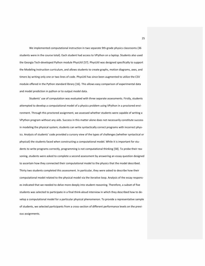
We implemented computational instruction in two separate 9th-grade physics classrooms (36

students were in the course total). Each student had access to VPython on a laptop. Students also used

the Georgia Tech-developed Python module PhysUtil [57]. PhysUtil was designed specifically to support

the Modeling Instruction curriculum, and allows students to create graphs, motion diagrams, axes, and

timers by writing only one or two lines of code. PhysUtil has since been augmented to utilize the CSV

module offered in the Python standard library [16]. This allows easy comparison of experimental data

and model prediction in python or to output model data.

Students’ use of computation was evaluated with three separate assessments. Firstly, students

attempted to develop a computational model of a physics problem using VPython in a proctored envi-

ronment. Through this proctored assignment, we assessed whether students were capable of writing a

VPython program without any aids. Success in this matter alone does not necessarily constitute success

in modeling the physical system; students can write syntactically correct programs with incorrect phys-

ics. Analysis of students’ code provided a cursory view of the types of challenges (whether syntactical or

physical) the students faced when constructing a computational model. While it is important for stu-

dents to write programs correctly, programming is not computational thinking [58]. To probe their rea-

soning, students were asked to complete a second assessment by answering an essay question designed

to ascertain how they connected their computational model to the physics that the model described.

Thirty two students completed this assessment. In particular, they were asked to describe how their

computational model related to the physical model via the iterative loop. Analysis of the essay respons-

es indicated that we needed to delve more deeply into student reasoning. Therefore, a subset of five

students was selected to participate in a final think-aloud interview in which they described how to de-

velop a computational model for a particular physical phenomenon. To provide a representative sample

of students, we selected participants from a cross-section of different performance levels on the previ-

ous assignments.

26

2.2 Proctored assignment

For the proctored assignment, students attempted to develop a 2D computational model that

determined the location and velocity of a thrown baseball after a specified amount of time. Students

completed this model individually and without aid from their instructor. The proctored assignment was

deployed on an online homework system that can randomize the values given in problem statements.

Students were provided with a program scaffold that imported the necessary modules, created the

baseball and ground objects, and defined the integration loop structure. See appendix 3.4 for an exam-

ple of a program scaffold and a completed assignment. To complete the assignment successfully, stu-

dents would assign the appropriate initial conditions and complete the integration loop by employing

Euler-Cromer integration [52]. To facilitate students’ successful completion of this assignment, students

were given a “Code Checking Case” [59]. In the "Code Checking Case", students were provided with the

correct final position and velocity of the ball after the given time had elapsed. Students could use this

case to check if their program modeled the situation correctly. After completing the "Code Checking

Case" students modeled a similar physical situation for the “Grading Case”. In the "Grading Case", the

initial conditions were altered including the integration time and the system was moved from the Earth

to the surface of the moon to reduce gravity. Answers were not provided for the "Grading Case." Stu-

dents input their final answers for the baseball’s final location and velocity and uploaded their code to

the homework system.

We sought to determine students’ success rates and if their struggles were due to challenges

with physics or with computational modeling. We started with codes that were developed to analyze

student code of orbital motion in the introductory physics class at Georgia Tech [59]. These codes are

split into five groups concerning different concepts: initial conditions, force calculation, updating New-

ton's 2nd law, and "other" concerning coding errors. New codes were suggested during the coding pro-

cess. The entire code set can be found in Table 8.

27

Table 8: Codes validated in previous work used for the proctored assignment [59]. Codes marked with asterisks(*) were not

applicable to the proctored assignment. GT students who were tasked with modeling the motion of planets became con-

fused when trying to select the appropriate exponent of the interaction constant [59]. This issue does not arise when model-

ing projectile motion and thus IC5 was not needed. In orbital motion, an explicit separation vector is required due to the

nature of motion (i.e., where is the separation vector and not necessarily zero), GT students attempted to raise this to a

power (when in fact it is the magnitude of the difference that should be raised not the vector) [59]. In projectile motion the

separation vector is always zero therefore there is never a need to interact with it (this is the excluded FC3). Due to the sim-

plicity of the forces involved in the proctored assignment students didn't have any other force direction confusion (the only

force direction would be the direction of gravity) thus FC5 was inapplicable. Using Euler-Cromer integration to represent

Newton's 2nd law programmatically, students modeling orbital motion often had difficulties differentiating between when

to use a scalar or a vector [59]. Since the acceleration is one dimensional in projectile motion SL3 was not needed. SL4 was in

regards to momentum updates and the proctored assignment does not consider momentum in its calculations (students

were told force is not the more general ) [59]. In projectile motion, the "massive particle" is the Earth. Generally, Newton's

theory of gravitation will work for this situation. However this can be reduced to for projectile motion and this is done for

the proctored assignment removing the need for O1.

Code Description

IC1 Student used all the correct given values from the grading case

IC2 Student used all the correct values from the test case

IC3 Student used the correct integration time from either the grading

case or test case.

IC4 Student used mixed initial conditions

IC5* Students confused the exponents on the units of the exponent of k

(interaction constant).

FC1 The force calculation was correct

FC2 The force calculation was incorrect, but the calculation procedure

was evident.

FC3* The student attempted to raise the separation vector to a power

FC4 The direction of the force was reversed

SL1 Newton’s second law was correct

SL2 Newton’s second law was incorrect but in a form that updates

SL3* Newton's second law was incorrect and the student attempted to

update it with a scalar force

SL4* Student created a new variable for p_f (momentum)

O1* Student attempted to update force, momentum, or position for

the massive particle.

O2 Student did not attempt the problem

O3 Student did not print final results

O4 Coding Error [60]

SUG1 Student didn't change anything inside the while loop

SUG2 Student created extra while loops

SUG3 Student printed in while loop

SUG4 Student did not indicate Newton's 2nd law causes a change in mo-

tion

Several of the codes needed to be dropped because they didn't apply, specifically, some issues

were not seen due to the high school students having an easier assessment problem. The Georgia Tech

(GT) students modeled the motion of orbiting planets, the high school students modeled the motion of a

28

baseball flying through the air. Two of these codes deal explicitly with vector issues that only arise with

complex problems like orbital motion (FC3, SL3). GT students were required to model momentum which

was not required for high school students, thus O1 was jettisoned. Finally, the GT students needed to

define the exponent of the separation constant which is not necessary for projectile motion (code IC5

and FC3).

The process for applying these codes had multiple steps and was based on producing high corre-

lation across two coders. Working with another graduate student, a small selection of proctored as-

signments were first analyzed using the codes from previous Georgia Tech work [59]. Examples and def-

initions of each code were developed from a subset of the high school student coding assignments. The-

se codes were applied to the entire data set. Cross correlation between codes at this stage indicated a

low agreement across all of the data set so the smaller data set selection was revisited. This process was

repeated until a high agreement between coders was reached. This process also generated new codes

labeled SUG# in Table 8. SUG1-4 all arose from how students wrote code within the while loop. SUG1-3

are computational idiosyncrasies that were interesting and merit further exploration. SUG4 is interesting

because students were explicitly instructed to define accelerations in their code in terms of force. Thus

SUG4 happens when students eschew this for simply writing the acceleration, in this case 2

m9.8

sg =

or 2

0,9.8s

,0 m

g ⟨ ⟩= .

To calculate the agreement between coders we tabulated the total number of agreements we

had (that is, the total number of times that two coders agreed that a code applied). Then we counted

the number of total codes. For example, if researcher A gave three unique codes to a student, and re-

searcher B gave two unique codes to a student, and researcher B's codes were contained within re-

searcher A's codes than they would disagree 1/3 of the time. Likewise, if researcher A gave two unique

codes and researcher B gave three unique codes but they only agreed once, the student would receive

29

four unique codes total and the researchers disagreed twice. The ratio of the total number of agree-

ments to the total number of unique codes gives the fractional agreement (that is, the inter-rater relia-

bility). In this case researchers agreed 83.8% of the time [61].

Our analysis of student python code suggests that high school students can engage in computa-

tional modeling in the context of physics and that these students are generally capable of using numeri-

cal computation to solve physics problems. Based on the output of their computational models, stu-

dents were placed into one of three categories: “correct results and animation” (N = 10, 31%), “pro-

duced animation, but incorrect results” (N=8, 25%), and “produced no animation” (N=14, 44%). The

group that produced an animation but had incorrect results could be broken down into two groups.

They either produced some number of errors either writing the integration algorithm alone (25%) or

writing the integration algorithm and assigning initial conditions (75%). The remaining 44% who pro-

duced no animation were split into two groups. They either had small syntactic errors (36%) or had nu-

merous physics and computational errors (64%). The group that had small syntactic errors most often

would have succeeded with minimal input from peers or instructors because these errors were minute

(e.g., missing a colon at end of while loop declaration but the rest of the program is correct).

The success rate here is important to note for several factors. First, the students had only spent

the fall semester learning to use computation. During this semester students only had two full activities

that had computation integrated. They then had a month long holiday break where they did not partici-

pate in any classroom activities. Upon returning the students had two weeks of beginning of year exam-

inations that did not include any material on computation. After this two weeks the students had a short

refresher (<1 day) on the Fall semester's material and then participated in the proctored assignment.

Thus students, had at least a 6 week gap between the education period (i.e., the fall semester where

they were learning to use computation in the context of force and motion) and the testing period. Four

of these weeks were not spent participating in educational instruction at all. Furthermore, in an informal

30

survey given by the classroom teacher indicates most students feel comfortable with the computer but

have no programming experience with the computer. Thus, high school students with little program-

ming experience can spend a relatively short period of time learning computation and a sizeable fraction

will be able to apply this knowledge in context at a later time. With more instruction and more integra-

tion, a more favorable portion of the class could complete this assessment successfully. But do these

students who complete code successfully understand it's link to the physics they are modeling? Or have

they simply memorized algorithms that can only be used in very specific contexts.

2.3 Essay questions

The code that students wrote for the proctored assignment demonstrated a variety of possible

outcomes, but this assessment was unable to probe deeply how students constructed these computa-

tional models. To look more deeply we asked the students to write a short essay. Students responded

to this essay question after they completed the proctored assignment. The essay question investigated

whether students’ success was predicated on simply reproducing an algorithm, or whether successful

students made deeper connections between the physics and the computational algorithm. That is, did

these students engage in the practice of computational thinking while developing their computational

model? The question given to the students probed the student understanding of how the computer in-

teracts with Newton's 2nd law via the Euler-Cromer integration. Twenty-nine of 32 students completed

the essay question. Students could run a working version of the program before answering the essay

question.

The practice of computational thinking requires a logical problem solving approach that often

involves thinking iteratively [59]. To further investigate how students developed their computational

models, we asked students to describe the integration (while) loop mathematically, physically, and pro-

grammatically. Specifically, the students were asked, "Download and run the completed baseball.py

program. What is the purpose of the loop? How can you describe (mathematically or physically) what

31

the loop does in your program? Run the program again and explain what the loop is doing while your

program is running." In order to provide a complete explanation, students needed to comment on the

iterative procedure of the loop itself and its relationship to the integration of the equations of motion by

the incremental stepping of Newton’s Second Law.

Three researchers catalogued all views that "arose" from the student responses. These views

formed codes that were tested against a small subset (<5) of essays. This process was repeated until an

agreement was formed on which codes applied where within the subset of essays. These codes were

then applied to all of the submitted essays. This process was repeated until there was a high agreement

between coders (100%).

Figure 5: Students who displayed Force-casual and Iterative views were more likely to be successful on the proctored as-

signment (N=29). The bars represent a total proportion of the class (that is out of 100%). The percentages in this graph are

32

different than the proctored assignment because the number of students who responded to the essays is slightly less (proc-

tored assignment N=32).

The explanations presented by students in response to this question were captured by four dis-

tinct but not necessarily exclusive views. Some (38%) students presented a “force-causal” view of the

loop structure. This view was characterized by a clear connection between force and motion. A student

presenting a force-causal view would describe how the force of gravity causes a change in the motion of

the ball; “The loop is constantly changing the velocity of the ball while the Fnet [net force] stays con-

stant. [The force] makes the ball fall faster with every loop that runs”. Another group (17%) of students

presented a “kinematic-observational” view of the loop structure. These students indicated they had

observed an acceleration (or some change in a kinematic quantity), but these students did not connect

this observation back to the concept of a non-zero net force. One student with a kinematic-

observational view noted, “The loop's purpose is to use the acceleration of the ball to affect the ball's

velocity and position. The loop is run every .01 seconds (deltat). It re-updates the velocity and position of

the ball at that interval.” Almost two-thirds (65%) of students described the integration loop as a local,

iterative process governed by instantaneous influences. This iterative-local view was characterized by a

discussion of incremental steps through the loop and statements such as “in this program, the [integra-

tion] loop is what the computer runs through to [compute] a new position, velocity, and all other forces

for every [time it executes].” All the students who exhibited a force-causal view and nearly all students

who presented a kinematic-observational view of motion also exhibited an iterative-local view of mo-

tion. Slightly more than a quarter (28%) of all respondents fell into no category. This group of students

most often wrote very short, incomplete responses that were too difficult to classify. More examples of

student essay coding can be found in Table 9.

33

Table 9:Student views with examples. Underlined portions indicate sections coded as applying to the associated view. Exam-

ples might include multiple views but this in not included in these examples.

Student View Example

Iterative procedures The program goes through all the steps and

prints/runs them while the "while" statement is

still true. While the program is running the loop is

going through the steps very fast.

Force-Causal (i.e., mentions force and motion

quantities together)

In this program the loop is what the computer runs

through to put in a new position, velocity and all

other forces for every .01 seconds. It is similar to a

movie in that in a movie there are a bunch of pic-

tures that scroll so quickly it looks like it is moving.

When it is running it moves the ball and updates

the time.

Kinematic-observational The loop shows the changes in every vector as the

time changes. I didn't really finish the vpython

module so I don't completely understand every-

thing yet. It also labels where the ball is at each

second.

No category No example

We compared the views that students presented on the essay question to their performance on

proctored coding assignment. Students with each view were binned into the broad proctored assign-

ment categories (i.e., “correct results and animation”, “produced animation, but incorrect results”, and

“produced no animation”). Students who presented both an iterative-local and force-causal view were

most likely to produce a correct program. Students whose essay were short and incomplete were most

likely to write programs that produced no animations. Figure 5 summarizes our findings.

2.4 High School Student Interviews

Students’ essay responses elucidated that the concepts of force, motion, and iterative processes

should be connected to facilitate computational thinking. However, investigating how students make

these connections requires observing and questioning students while they engage in the practice of

computational thinking. Several weeks after students completed the essay question, we interviewed five

of them while they filled in the missing pieces of a scaffolded computational modeling program on pa-

per. During the interview, students also answered questions about how they define a force and how

34

forces, motion, and the integration loop are related. Students were asked to speak out loud while com-

pleting the scaffolded code and answering questions; their responses were videotaped. Only students

whose proctored assignment code produced animations (i.e., “correct results and animation” and “pro-

duced animation, but incorrect results”) were invited to the study. Six students were chosen to partici-

pate; five completed the interview. Of the students who completed the interview, 3 presented force-

causal and iterative-local views on the essay question. One student had previously presented both a kin-

ematic-observational and an iterative-local view, but expressed a force-causal and an iterative-local view

in the interview. The last student presented a primarily iterative-local view on the essay question and in

the interview.

For students who developed a correct computational model, the interviews further highlighted

the links they made between force, motion, and iterative processes. A student who wrote a correct pro-

gram described her code with a force-causal and an iterative-local view, “To predict the velocity you

would have to do baseball.v = initial velocity of the baseball plus gravity times time. That would give me

the new velocity after [the execution of] every single loop. And then you need to update the position

based on the loop.” This student presents the basic concepts behind Newton’s 2nd law but also de-

scribes how the numerical integration loop updates the velocity of the ball in each execution. By con-

trast, a student who constructed a model that produced incorrect animation demonstrated an incorrect

conception of force and motion, “force generally [is] acquired through motion. There's always force act-

ing on an object.” When questioned about how the loop models the physics of the system, the student

presented solely an iterative-local view, “[the loop] has formulas that it solves for, like, update position

equals [baseball.pos + baseball.v*deltat].” While this student was able to generate a

computational model for the proctored assignment that ran without (syntactic) errors, she did not use

the correct physics to do so.

35

3 CONCLUSIONS

3.1 Discussion

The results of this preliminary study are promising. 9th grade students with little to no pro-

gramming experience were able to complete physics computational models to some (~31% totally cor-

rect) degree of proficiency. This raises the question, "What defines success?" In this implementation,

there were many decisions made by the experimenters that impacted the overall success of the stu-

dents. Students spent very little time in class actually programming. There were only two computational

assignments given to the entire class. There was also no link between experiment and computational

model building. These two choices are probable causes for the low "total success" number. However,

given the time between the educational period and the assessment period (6-8 weeks) and the success

rate (31% wrote completely correct programs), the results seem more positive than they would at first

glance. The 31% success rate indicates that students in high school can learn a computational tool like

python in the context of physics (with effort). This is reinforced by the fact that the majority of students

(86%) had little to no background in programming. Thus, it behooves future researchers to carry out

work that extends computation throughout the curriculum.

It is important to note the background of the students in this study. The high school in this study

is a private day school in Georgia. While students were not directly asked for their parents income lev-

els, some assumptions can be made about the socio-economic status of the students based on data col-

lected with the technology survey. Twenty percent of the students had iPads (in 2011, the iPad had been

out for less than two years and 8.9% of the population possessed one), 56% of the students had their

own smartphone, 78% had their own laptop (60% of which were MacBooks), and all students had high-

speed internet access at home [62]. While not a conclusive measure of socio-economic status, these

data do suggest that students at the high school are affluent. Thus, their classroom performance could

tend towards success more often than that of a student with lower socioeconomic status (SES) [63]. Fur-

36

ther work must be done to make these curriculum transformations accessible to all students, regardless

of socio-economic status.

Another variable that could affect student success is the classroom teacher's level of compe-

tence at computational modeling. Jackson reports that students are more successful with teachers that

have been labeled "master modelers" in Modeling Instruction classrooms [9]. This reasoning could ex-

tend to teaching computational modeling as well. The classroom teacher has an MS in Physics with sev-

eral years of experience in Python programming. He also had the support of a research group of PhD

students, physics professors, and researchers whose focus was on teaching computational physics. Can

less experienced teachers still see success in their classrooms with some training? What level of support

will these teachers need? It stands to reason that initially these teachers will need previously generated

activities and a framework to offer these activities. Community and departmental support will also be a

must for these teachers.

One of the stated goals of teaching physics with computation is for students to understand that

motion can be described with Newton's 2nd law. In Python code, initial conditions are first explicitly de-

clared, then calculations are performed. If a student were to add another force to the model, this would

be an explicit action on the student’s part. Our analysis of the essays begins to show that students are

thinking this way. Students who had a good understanding of how the computer interacted with the

physics were better at producing successful code (see Figure 5). To further explore this connection, stu-

dents should be challenged with a problem that is beyond their educational experience. For instance,

one might give a student a problem to model with a mix of forces, like a ball rolling down a hill, falling

into the ocean, then eventually settling on the ocean floor. If a student could a) describe the forces at

each step, and b) describe the code that would model this situation, this could demonstrate change in a

study which compares students in a traditional physics class to this group.

37

Students also need to see computation as a tool for solving physics. This question was not as-

sessed in this research. Students’ reactions to using computation is important because we want them to

not only learn to use the tool, we want them to understand why it is important to learn the tool at all.

Science class should be about practicing what scientists do. In conversations with classroom teachers at

the pilot high school, students have described a disconnect between computation and physics [64]. This

was an unfortunate outcome that may be due to the way computation was implemented in the MI cur-

riculum.

3.2 Looking Back

Ninth grade students were exposed to the scientific practices of modeling and computation.

Making science education more like science practice produces students better equipped to solve mod-

ern day problems [6, 25, 38]. Some students in this study demonstrated that in learning the scientific

practices of modeling and computation, they extended their sense making. Students who competently

produced programs were most likely to describe these models as a representation of a causal relation-

ship between force and motion change. This corroborates previous research in the use of computation

in the physics classroom [65-67]. High school students writing code also demonstrated problem-solving

difficulties similar to the difficulties exhibited by undergraduate students [59]. Thus, academic maturity

may not play a role in learning computation, at least in students who are adolescents or older. Confirm-

ing and expanding the results of this thesis will require more test classrooms and teacher support.

3.3 Looking Forward

Implementing course reform is never easy. Instructors report motivations for implementing re-

search based instructional strategies ranging from "it was easy" to "motivated by evidence" [68]. Many

instructors do not possess the skills to do computation themselves and need instruction to support im-

plementing computation in their courses [11]. Integrating computation into a curriculum also requires

38

the jettisoning of other knowledge or skills that could be covered [65]. Anecdotally, students buck at

curriculum change, which can cause instructors to hesitate. This has been noted by teachers at the pilot

high school [64]. Discussions with these teachers indicates this may be due to a poor link between com-

putational modeling and predicting experimental observations.

In this implementation, the computational component was kept separate because it was only in-

troduced to the students during the model deployment stage. The students would do an experiment,

discuss it in class, and expand it with additional assignments. They then would work on a computational

assignment that was related to the initial experiment. The classroom instructor would have a discussion

about the predictive power of computation, but this would never be strongly linked back to the experi-

ment. Future implementations should have a stronger link between the experiment/observation and the

computational prediction. This would involve actually predicting experimental values with the computa-

tional model, then testing the accuracy of these models. This process would more closely resemble real

scientific practice, and is currently being tested at the college level and with an online course [69].

Student sense-making while modeling with computation should be further developed. In this

study, many successful students demonstrated that they did more than memorize an algorithm in their

solution-making. How do these students organize this knowledge cognitively? How do they access it

when they solve problems? If we can characterize this process, can we operationalize it and teach it to

other students? Working with both high school students and college students, instructors note students

often resist "tweaking" models. Students often stop at descriptions that are not physical. What factors in

students knowledge's and skill sets lead them to wrong conclusions? How can we strengthen students

meta-cognitive abilities that allow them to "tweak" more effectively?

39

REFERENCES

1. J. P. Holden, “Engage to excel: Producing one million additional college graduates with

degress in science, technology, engineering, and mathematics,” 2012.

2. J. Casner-Lotto and M. W. Benner, “Are they really ready to work? Employers

Perspectives on the Basic Knowledge and Applied Skills of New Entrants to the 21st

Century U.S. Workforce,” The Conference Board, Inc., 2006.

3. H. e. a. Quinn, A Framework for K-12 Science Education: Practices, Crosscutting

Concepts, and Core Ideas, The National Academies Press, 2012.

4. E. F. Redish, “Student programming in the introductory physics course: M.U.P.P.E.T.,”

The American Journal of Physics, pp. 61:222-232, 1993.

5. W. K. Adams, K. K. Perkins, N. Podolefsky, M. Dubson, N. D. Finkelstein and C. E.

Wieman, “A new isntrument for measuring student beliefs about physics and learning

physics: The Colorado Learning Attitudes about Science Survey,” Physical Review

Special Topics - Physics Education Research, 2006.

6. A. Karelina and E. Etkina, “Acting like a physicist: Student approach study to

experimental design,” Physical Review Special Topics - Physics Education Research,

2007.

7. Achieve, Inc., “The Next Generation Science Standards,” 2013. [Online]. Available:

http://www.nextgenscience.org/next-generation-science-standards. [Accessed 21 June

2013].

8. D. Hestenes, “Findings of the modeling workshop: 1994-2000,” National Science

40

Foundation, 2000.

9. J. Jackson, “Modeling instruction: An effective model for science education,” Science

Educator, 2008.

10. I. A. Halloun, Modeling theory in science education, Netherlands: Kluwer Academic

Publishers, 2004.

11. N. Chonacky and D. Winch, “Integrating comutation into the undergraduate

curriculum: A vision and guidelines for future developments,” American Journal of

Physics, pp. 327-333, 2008.

12. D. S. M. C. Klahr, “Cognitive Objectives in a LOGO Debugging Curriculum: Instruction,

Learning, and Transfer,” Cognitive Psychology, pp. 362-404, 1988.

13. B. K. Nastasi and D. H. Clements, “Effectance motivation, percieved scholastic

competence, and higher-order thinking in two cooperative computer environments,”

Journal of Educational Psychology, pp. 10:249-275, 1994.

14. D. Scherer, P. Dubois and B. Sherwood, “VPython: 3D interactive scientific graphics for

students,” Computing in Science and Engineering, pp. 82-88, 2000.

15. “vpython.org,” 2013. [Online]. Available: http://vpython.org. [Accessed 10 June 2013].

16. “PhysUtil v.1.25.1,” 2013. [Online]. Available: https://code.google.com/p/python-

physutil/downloads/list.

17. R. D. Knight, Five easy lessons: Strategies for successful physics teaching, San

Francisco: Addison Wesley, 2004.

18. “What is Modeling Instruction?,” 2013. [Online]. Available:

http://modelinginstruction.org/researchers/publications/what-is-modeling-

41

instruction/. [Accessed 16 June 2013].

19. American Modeling Teachers Association, “American Modeling Teachers Association,”

2013. [Online]. Available: http://modelinginstruction.org/. [Accessed 21 June 2013].

20. Nobel Media AB, “All Nobel Laureates in Physiology or Medicine,” 2013. [Online].

Available: http://www.nobelprize.org/nobel_prizes/medicine/laureates/. [Accessed 21

June 2013].

21. A. F. Strassberg and L. J. Defelice, “Limitations of the Hodgkin-Huxley formalism:

Effects of the single channel kinetics on transmembrane voltage dynamics,” Neural

Computation, pp. 843-855, 1993.

22. D. L. Turcotte and G. Schubert, Geodynamics, Cambridge: Cambridge University Press,

2002.

23. M. Schober, 2010. [Online]. Available: http://modelinginstruction.org/wp-

content/uploads/2012/04/Mechanics-Unit-2-sample-.pdf. [Accessed 16 June 2013].

24. Modeling Workshop 2002, “Motion Maps,” 2002. [Online]. Available:

http://teachernotes.paramus.k12.nj.us/ning/images/documents/cycle1-

5/09_U2%20reading.pdf. [Accessed 8 August 2013].

25. E. Brewe, L. Kramer and G. O'Brien, “Modeling instruction: Positive attitudinal shifts in

introductory physics measured with C-LASS,” Phys. Rev. ST Phys. Educ. Res., 2009.

26. D. Hestenes, M. Wells and G. Swackhamer, “Force Concept Inventory,” The Physics

Teacher, pp. 141-158, 1992.

27. M. D. Caballero, J. B. Burk, J. M. Aiken, S. S. Douglas, E. M. Scanlon, B. D. Thoms and M.

F. Schatz, “Integrating Numerical Computation into the Modeling Instruction

Curriculum,” The Physics Teacher, p. Accepted, 2013.

42

28. V. Sawtelle, E. Brewe and L. H. Kramer, “Positive impacts of modeling instruction on

self-efficacy,” in Physics Education Research Conference 2010, Portland, 2010.

29. M. Wells, D. Hestenes and G. Swackhamer, “A modeling method for high school

physics instruction,” American Journal of Physics, pp. 606-619, 1994.

30. L. L. Liang, G. W. Fulmer, D. M. Majerich, R. Clevenstine and R. Howanski, “The effects

of a model-based physics curriculum program with a physics first approach: A causal-

comparitive study,” Jorunal of Science Education and Technology, pp. 114-124, 2012.

31. A. Bandura, “Self-efficacy: Toward a Unifying Theory of Behavioral Change,”

Psychological Review, pp. 191-215, 1977.

32. H. S. Fencl and K. R. Scheel, “Pedagogical approaches, contextual variables, and the

development of student self-efficacy in undergraduate physics courses,” Physics

Education Research Conference Proceedings, pp. 173-176, 2003.

33. M. J. O'Brien and J. R. Thompson, “Effectiveness of ninth-grade physics in Maine:

Conceptual understanding,” The Physics Teacher, pp. 234-239, 2009.

34. D. A. Stainforth, “Uncertainty in the predictions of the climate response to rising levels

of greenhouse gases,” Nature, pp. 433:403-406, 2005.

35. D. H. Boal and J. N. Glosli, “Computational model for nuclear reaction studies:

Quasiparticle dynamics,” Phys. Rev. C, pp. 2621-2629, 1988.

36. D. W. Nixon, 2013. [Online]. Available: http://www.mathworks.com/aerospace-

defense/miadc/presentations/10_F35_Flight_Control_DevelopmentDaveNixon.pdf.

[Accessed 13 March 2013].

37. M. Prensky, “Digital Natives, Digital Immigrants,” On the Horizon, 2001.

43

38. R. Ivie and K. Stowe, “The Early Careers of Physics Bachelors,” American Institute of

Physics, College Park, 2002.

39. D. Hagan and S. Markham, “Does it help to have some programming experience before

entering a computing degree program?,” Proceedings of the 5th annual SIGCSE/SIGCUE

ITiCSEconference on Innovation and technology in computer science education, pp. 25-

28, 2000.

40. M. A. Kohlmeyer, M. D. Caballero, R. Catrambone, R. W. Chabay, L. Ding, M. P. Haugan,

M. J. Marr, B. A. Sherwood and M. F. Schatz, “Tale of two curricula: The performance

of 2000 students in introductory electromagnetism,” Physical Review Special Topics -

Physics Education Research, 2009.

41. J. Ives, Personal communication, 2013.

42. A. Rundquist, Standards-Based Grading with Voice: Listening for Students’

Understanding, Nebraska: Physics Education Research Conference 2011 Dinner

Speaker, 2011.

43. D. H. Clements, “Enhancement of creativity in computer environments,” American

Educational Research Journal, pp. 28:173-87, 1991.

44. B. K. Nastasi, D. H. Clements and M. T. Battista, “Social-cognitive interactions,

motivation, and cognitive growth in Logo programming and CAI problem-solving

environments,” Journal of Educational Psychology, pp. 82:150-58, 1990.

45. A. Waytz, C. K. Morewedge, N. Epley, G. Monteleone, J.-H. Gao and J. T. Cacioppo,

“Making sence by making sentient: Effectance motivation increases

anthropomorphism,” Journal of Personality and Social Psychology, pp. 99:3,410-435,

2010.

44

46. S. F. Railsback, S. L. Lytinen and S. K. Jackson, “Agent-based simulation platforms:

Review and development recommendations,” Simulation, pp. 609-623, 2006.

47. “NumPy,” 2013. [Online]. Available: http://www.numpy.org/. [Accessed 24 January

2013].

48. “SciPy,” 2013. [Online]. Available: http://www.scipy.org/. [Accessed 24 January 2013].

49. TIOBE Software, “TIOBE Programming Community Index for June 2013,” June 2013.

[Online]. Available:

http://www.tiobe.com/index.php/content/paperinfo/tpci/index.html. [Accessed 18

June 2013].

50. B. A. a. R. C. Sherwood, “VPYTHON: 3D PROGRAMMING FOR ORDINARY MORTALS,” in

MPTL14, Udine, 2009.

51. R. Beichner and M. H. Dancy, “Impact on animation on assessment of conceptual

understanding in physics,” Physical review special topics physics education research,

2006.

52. A. Cromer, “Stable solutions using the euler approximation,” American Journal of

Physics, 1981.

53. J. M. Aiken, M. D. Caballero, S. S. Douglas, J. B. Burk, E. M. Scanlon, B. D. Thoms and M.

F. Schatz, “Understanding Student Computational Thinking with Computational

Modeling,” in Physics Education Research Conference 2012, Philadelphia, 2012.

54. J. B. Burk, “Computational Modeling,” 2011. [Online]. Available:

http://quantumprogress.wordpress.com/computational-modeling/. [Accessed 21 June

2013].

55. D. Brown, “Tracker: Video Analysis and Modeling Tool,” 2013. [Online]. Available:

45

http://www.cabrillo.edu/~dbrown/tracker/. [Accessed 5 June 2013].

56. J. B. Burk, Personal Correspondence, 2013.

57. “PhysUtil v1.22,” Atlanta, 2010-2012.

58. J. Wing, “Computational Thinking,” Communications of the Association for Computing

Machinery, pp. 49:3:33-35, 2006.

59. M. D. Caballero, M. A. Kohlmeyer and M. F. Schatz, “Fostering computational thinking

in introductory mechanics,” in AIP Conference Proceedings. Vol. 1413, 2012.

60. Microsoft Corporation, “Know your bugs: Three kinds of programming errors,” 2013.

[Online]. Available: http://msdn.microsoft.com/en-us/library/s9ek7a19(v=vs.80).aspx.

[Accessed 3 June 2013].

61. K. D. Multon, “Interrater Reliability,” in Encyclopedia of Research Design, Thousand

Oaks, CA, SAGE Publications, Inc., 2010, pp. 627-629.

62. eMarketer, "iPad Use to Nearly Double This Year," eMarketer, 11 June 2012. [Online].

Available: http://www.emarketer.com/Article/iPad-Use-Nearly-Double-This-

Year/1009106. [Accessed 13 August 2013].

63. R. H. Hadley and R. F. Corwyn, “Socioeconomic status and child development,” Annual

Review of Psychology, pp. 371-399, 2002.

64. M. Hayes-Golding, Personal Communication, 2013.

65. R. Chabay and B. Sherwood, “Computational physics in the introductory calculus-based

course,” American Journal of Physics, pp. 307-313, 2008.

66. M. D. Caballero, Evaluating and Extending a Novel course Reform of Introductory

Mechanics, Atlanta, GA, 2011.

46

67. M. A. Kohlmeyer, Student performance in computer modeling and problem solving in a

modern introductory physics course, Pittsburgh, 2005.

68. M. H. Dancy, C. Turpen and C. Henderson, “Why do faculty try research based

instructional strategies?,” in Physics Education Research Conference, 2010.

69. M. M. Waldrop, “Education online: The virtual lab,” Nature, vol. 499, no. 18 July 2013,

p. 268–270, 2013.

70. L. Grandell, M. Peltomäki, R.-J. Back and T. Salakoski, “Why complicate things?

Introducing programming in high school using Python,” ACE '06 Proceedings of the 8th

Australasian Conference on Computing Education, pp. 71-80, 2006.

71. M. F. Schatz, “Your World is Your Lab,” 2013. [Online]. Available:

https://class.coursera.org/phys1-001/class. [Accessed 5 June 2013].

72. J. M. Roschelle, R. D. Pea, C. M. Hoadley and D. N. Gordin, “Changing How and What

Children Learn in School with Computer-Based Technologies,” The Future of Children,

Vol. 10, No. 2, Children and Computer Technology, pp. 76-101, 2000.

73. D. Halliday, R. Resnick and J. Walker, Fundamentals of Physics, John Wiley & Sons, Inc.,

1997.

74. N. Finkelstein, “When learning about the real world is better done virtually: A study of

substituting computer simulations for laboratory equipment,” Physical Review Special

Topics - Physics Education Research, 2005.

75. K. E. Gray, W. K. Adams, C. E. Wieman and K. K. Perkins, “Students know what

physicists believe, but they don't agree: A study using the CLASS survey,” Physical

Review Special Topics - Physics Education Research, 2008.

76. R. W. Chabay and B. A. Sherwood, Matter and Interactions, Wiley, 2010.

47

77. M. D. Caballero, M. A. Kohlmeyer, E. F. Greco, E. R. Murray, K. R. Bujak, M. J. Marr, R.

Catrambone and M. F. Schatz, “Comparing large lecture mechanics curricula using the

Force Concept Inventory: A five thousand student study,” American Journal of Physics,

p. 638, 2012.

78. D. M. Kurland and R. D. Pea, “Children’s Mental Models of Recursive LOGO Programs,”

Journal of Educational Research, pp. 235-243, 1985.

48

APPENDICES

3.1 Reasons for Choosing Python as a Learning Language

Table 10 : This table has been reproduced from [70].

Feature Reason

Small and clean syntax Compared to languages such as Java or C++, Py-

thon has a more intuitive syntax.

Example Hello World program:

Python:

Print "Hello World!"

Java: class Hi {

public static void main (String

args[]) {

System.out.println("Hi!");

}

}

% javac Hi.java

% java Hi

Dynamic typing Python is dynamically typed, which further reduces

the notation.

Expressive semantics Python's basic types are powerful: for example,

lists can be introduced at the same time as other

built-in types.

Immediate feedback The interpreter enables fast and interactive

demonstration of programming concepts, and

gives immediate and understandable feedback on

potential errors.

Enforced structural design Python enforces an indented and structured way

of writing programs, and the code resembles

pseudo code.

Relevant open-source software Python is free and widely used. It comes with a

text editor (IDLE), and a large amount of tutorials,

books, course material, exercises, assignments and

extensive documentation is available on the web.

3.2 Computational Activities Designed and Used by John Burk

These activities can be found online at http://quantumprogress.wordpress.com/computational-

modeling/. While the activities report (at the bottom) that they were part of the 2006 Modeling Work-

49

shop Project, they were not developed for this project and the only relation to the project is our work

augmenting Modeling Instruction with computation.

3.2.1 Introduction to Computational ModelingIntroduction to Computational Modeling

50

51

3.2.2 WebAssign Constant Velocity Assignment

WebAssign is an online homework system

WebAssign Constant Velocity Assignment

WebAssign is an online homework system.

52

53

Computational Modeling Activity 2: Balanced ForcesComputational Modeling Activity 2: Balanced Forces

54

55

56

57

3.3 Student Technology Survey Results

Students were given an informal technology survey at the beginning of the school year. All stu-

dents had high speed internet access at home. In addition to the school provided laptops 24 (out of 36)

students had laptops they brought to school with them every day.

While this is an informal survey several comments can be made about the results due to the de-

sign. The question "how comfortable are you with the computer?" has a three point scale response

where the vast majority of the students picked the middle response. Survey design research has show

that on three point scales respondents often choose the middle response over lowest or highest re-

sponse. Thus, the design of this question may have biased the students. The granularity produced by the

question "Do you know anything about programming a computer?" is poor with a "Yes/No" response.

The question is also vague. A more appropriate way of gaining this information may be to split the ques-

tion into two parts. First ask the students to rate how comfortable they feel about their knowledge of

writing computer code on a five point scale (1 is very uncomfortable, 5 is very comfortable). Then, ask

the students to rate their experience with writing computer code on a five point scale (1 is no experi-

ence, 5 is expert level experience).

Only 20 out of 36 students responded "yes" to the question "Do you know anything about pro-

gramming a computer?" (in this context, "programming a computer" means writing code in any com-

puter language to produce a novel program or solution). In the follow up question asking students to

explain their experiences only one reported that they had an advanced level of programming experience

stating " I can code in Arduino [an embedded systems device] format very well and know bits and pieces

of java and C++". The other group reported that they had very little prior exposure to programming or

computation stating that the only experience was a brief period in 7th grade math using QBASIC (14).

This group made statements like, " Very limited knowledge: QBasic in 7th glade". See Table 7 : Students

58

were asked the question "Do you know anything about programming a computer?". If they responded

yes they were asked to explain their experiences (N=36).

Question Response

Do you have access to a computer high speed in-

ternet connection at home?

Yes

No

36

0

Do you have a laptop computer that you can

bring to school?

Yes, A Mac laptop

Yes, a Windows laptop

No, I don't have a lap-

top

No, I have a laptop, but

I can't bring it to school

15

9

8

4

Do you have a cell phone? Yes

No

35

1

Do you have a smartphone? iPhone 4

iPhone 3G

other iPhone

Android Phone

Blackberry

Other smartphone

No smartphone

7

7

1

3

1

1

16

Do you have an mp3 player? iPod Touch

iPod Nano

Other iPod

Other mp3 player

No mp3 player

20

2

12

1

1

Do you have a tablet computing device? iPad 1

iPad 2

Android tablet

No

6

1

0

29

What type of operating system does your com-

puter at home run?

Mac OS X 16

Windows XP 2

Windows Vista 4

Windows 7 6

How old is your computer? <6 months 7

6 months - 1 year 3

1-2 years 6

2-3 years 7

>3 years 5

How comfortable are you with a computer? not comfortable—I can

only do things if I'm

shown how, and don't

know what to do to fix

it.

3

comfortable—I can in- 29

59

stall/delete programs

and learn new applica-

tions on my own.

very comfortable—I'm

the one everyone calls

whenever the computer

needs to be fixed.

4

Do you know anything about programming a

computer?

Yes 20

No 16

Rate your experience with the following pro-

grams

program No experience

to basic expe-

rience

advanced to

expert experi-

ence

Word Proces-

sor (MS Word,

Pages)

7 29

Spreadsheet

(Excel)

15 21

Photo/Video

software

25 11

Google Docs 27 9

Please rate your familiarity with the following

web technologies

program No experience

to basic expe-

rience

advanced to

expert experi-

ence

Blogging 28 8

Twitter 31 5

Facebook 18 18

Search 8 28

Web Site De-

sign

32 4

3.4 Proctored Assignment

This appendix includes the scaffolded code that was given to the students during the proctored

assignment assessment as well as an example of what a completed computational model would look

like.

3.4.1 Code That was given to students at the beginning of the assessment

from __future__ import division

from visual import *

from physutil import *

from visual.graph import *

###SETUP Elements

60

#--------------------------------------------------------------

scene.title = 'Hit a home run!'

field = box(pos=vector(0,0,0),size=(122,10,50),color = color.green,opacity =

0.3)

baseball = sphere(radius=.5,color=color.red)

###SETUP PARAMETERS & INITIAL CONDITIONS

#--------------------------------------------------------------

baseball.pos = (-61,1,0)

baseball.m=.145 #mass in kg

baseball.v=vector(25,25,0)

ballparkwall = 122 #distance to outfield wall in m

gravity=vector(0,-9.8,0)

t=0

deltat=.01

tf = 10

###MOTION MAP

#--------------------------------------------------------------

motionMap = MotionMap(baseball, tf, 10, markerType="breadcrumbs",

labelMarkerOffset=vector(0,.3,0), dropTime=True)

###CALCULATION LOOP; perform physics updates and drawing

#--------------------------------------------------------------

while baseball.pos.x < ballparkwall and (baseball.pos.y)>field.pos.y: #while

the ball is inside the park

rate(100)

#Calculate forces

#update velocity

#update position

baseball.pos = baseball.pos + baseball.v*deltat

#update motionMap

motionMap.update(t)

#update time

t=t+deltat

###OUTPUT

#--------------------------------------------------------------

print t

61

3.4.2 An example of successful code

from __future__ import division

from visual import *

from physutil import *

from visual.graph import *

###SETUP Elements

#--------------------------------------------------------------

scene.title = 'Hit a home run!'

field = box(pos=vector(0,0,0),size=(122,10,50),color = color.green,opacity =

0.3)

baseball = sphere(radius=.5,color=color.red)

###SETUP PARAMETERS & INITIAL CONDITIONS

#--------------------------------------------------------------

baseball.pos = (-61,1,0)

baseball.m = .145 #mass in kg

baseball.v = vector(25,25,0)

ballparkwall = 122 #distance to outfield wall in m

gravity = vector(0,-9.8,0)

t=0

deltat=.01

tf = 10

###MOTION MAP

#--------------------------------------------------------------

motionMap = MotionMap(baseball, tf, 10, markerType="breadcrumbs",

labelMarkerOffset=vector(0,.3,0), dropTime=True)

###CALCULATION LOOP; perform physics updates and drawing

#--------------------------------------------------------------

while baseball.pos.x < ballparkwall and (baseball.pos.y)>field.pos.y: #while

the ball is inside the park

rate(100)

#Calculate forces

netforce = gravity*baseball.m #+ any other forces

#update velocity

baseball.v = baseball.v + netforce/baseball.m*deltat

#update position

baseball.pos = baseball.pos + baseball.v*deltat

#update motionMap

motionMap.update(t)

#update time

t=t+deltat

62

###OUTPUT

#--------------------------------------------------------------

print t

print baseball.v