HAL Id: hal-01104081https://hal.inria.fr/hal-01104081v2

Submitted on 19 Dec 2015

HAL is a multi-disciplinary open accessarchive for the deposit and dissemination of sci-entific research documents, whether they are pub-lished or not. The documents may come fromteaching and research institutions in France orabroad, or from public or private research centers.

L’archive ouverte pluridisciplinaire HAL, estdestinée au dépôt et à la diffusion de documentsscientifiques de niveau recherche, publiés ou non,émanant des établissements d’enseignement et derecherche français ou étrangers, des laboratoirespublics ou privés.

Optical flow modeling and computation: a surveyDenis Fortun, Patrick Bouthemy, Charles Kervrann

To cite this version:Denis Fortun, Patrick Bouthemy, Charles Kervrann. Optical flow modeling and computation: asurvey. Computer Vision and Image Understanding, Elsevier, 2015, 134, pp.21. hal-01104081v2

Optical flow modeling and computation: a survey

Denis Fortuna,∗, Patrick Bouthemya, Charles Kervranna

aInria, Centre de Rennes - Bretagne Atlantique, Rennes, France

Abstract

Optical flow estimation is one of the oldest and still most active research domains in computer vision. In 35 years, manymethodological concepts have been introduced and have progressively improved performances, while opening the way to newchallenges. In the last decade, the growing interest in evaluation benchmarks has stimulated a great amount of work. In this paper,we propose a survey of optical flow estimation classifying the main principles elaborated during this evolution, with a particularconcern given to recent developments. It is conceived as a tutorial organizing in a comprehensive framework current approachesand practices. We give insights on the motivations, interests and limitations of modeling and optimization techniques, and wehighlight similarities between methods to allow for a clear understanding of their behavior.

Keywords: Optical flow; Motion estimation; Regularization; Parametric models; Optimization; Feature matching, Occlusions.

1. Introduction

Motion analysis is one of the main tasks of computer vision.From an applicative viewpoint, the information brought by thedynamical behavior of observed objects or by the movementof the camera itself is a decisive element for the interpretationof observed phenomena. The motion characterizations can beextremely variable among the large number of application do-mains. Indeed, one can be interested in tracking objects, quan-tifying deformations, retrieving dominant motion, detecting ab-normal behaviors, and so on. The most low-level characteri-zation is the estimation of a dense motion field, correspondingto the displacement of each pixel, which is called optical flow.Most high-level motion analysis tasks employ optical flow as afundamental basis upon which more semantic interpretation isbuilt.

Optical flow estimation has given rise to a tremendous quan-tity of works for 35 years. If a certain continuity can be foundsince the seminal works of [120, 170], a number of methodolog-ical innovations have progressively changed the field and im-proved performances. Evaluation benchmarks and applicativedomains have followed this progress by proposing new chal-lenges allowing methods to face more and more difficult situ-ations in terms of motion discontinuities, large displacements,illumination changes or computational costs. Despite great ad-vances, handling these issues in a unique method still remainsan open problem. Comprehensive surveys of optical flow liter-ature were carried out in the nineties [21, 178, 228]. More re-cently, reviewing works have focused on variational approaches[267], benchmark results [13], specific applications [115], ortutorials restricted to a certain subset of methods [177, 260].

∗Corresponding author at Biomedical Imaging Group, Ecole PolytechniqueFederale de Lausanne (EPFL), CH-1015 Lausanne VD, Switzerland.

Email address: denis.fortun@epfl.ch (Denis Fortun)

However, covering all the main estimation approaches and in-cluding recent developments in a comprehensive classificationis still lacking in the optical flow field.

This survey paper is conceived as a tutorial aiming at orga-nizing in a comprehensive framework the main approaches andpractices for optical flow estimation. We will not try to tell thewhole story of optical flow evolution, neither we give an ex-haustive list of existing methods. We rather propose a syntheticclassification of the main methodological principles of exist-ing methods, with a particular concern given to recent develop-ments. We will insist on the modeling aspects, practical inter-ests and limitations of each introduced methodological element,with the aim of providing useful cues for a better understand-ing of optical flow. We adopt a classifying approach, decom-posing the optical flow estimation problem in sub-parts. Thisviewpoint has the advantage of being didactic and facilitatesthe identification of similarities between methods in a globalunique framework. However, this ambition of clarity shouldnot hide that individual methods are often conceived as coher-ent approaches, and cannot be reduced to a mere assembly ofisolated parts.

The remainder of this paper is organized as follows. In Sec-tion 2, we present general and basis concepts on optical flowused throughout the paper. Section 3 is devoted to a review ofdata constancy assumptions for optical flow and their usage forthe design of data terms. In Section 4, the parametric approach,its specific issues and existing solutions are described. Section5 presents the modelling and optimization aspects of globallyregularized methods. Section 6 focuses on the occlusion issue.Section 7 is dedicated to the recent trend of integrating featurematching in the optical flow estimation process. Finally, thegeneral conclusions of this survey are reported in Section 8.

Preprint submitted to Computer Vision and Image Understanding December 19, 2015

2. Preliminaries

2.1. Definition of optical flow

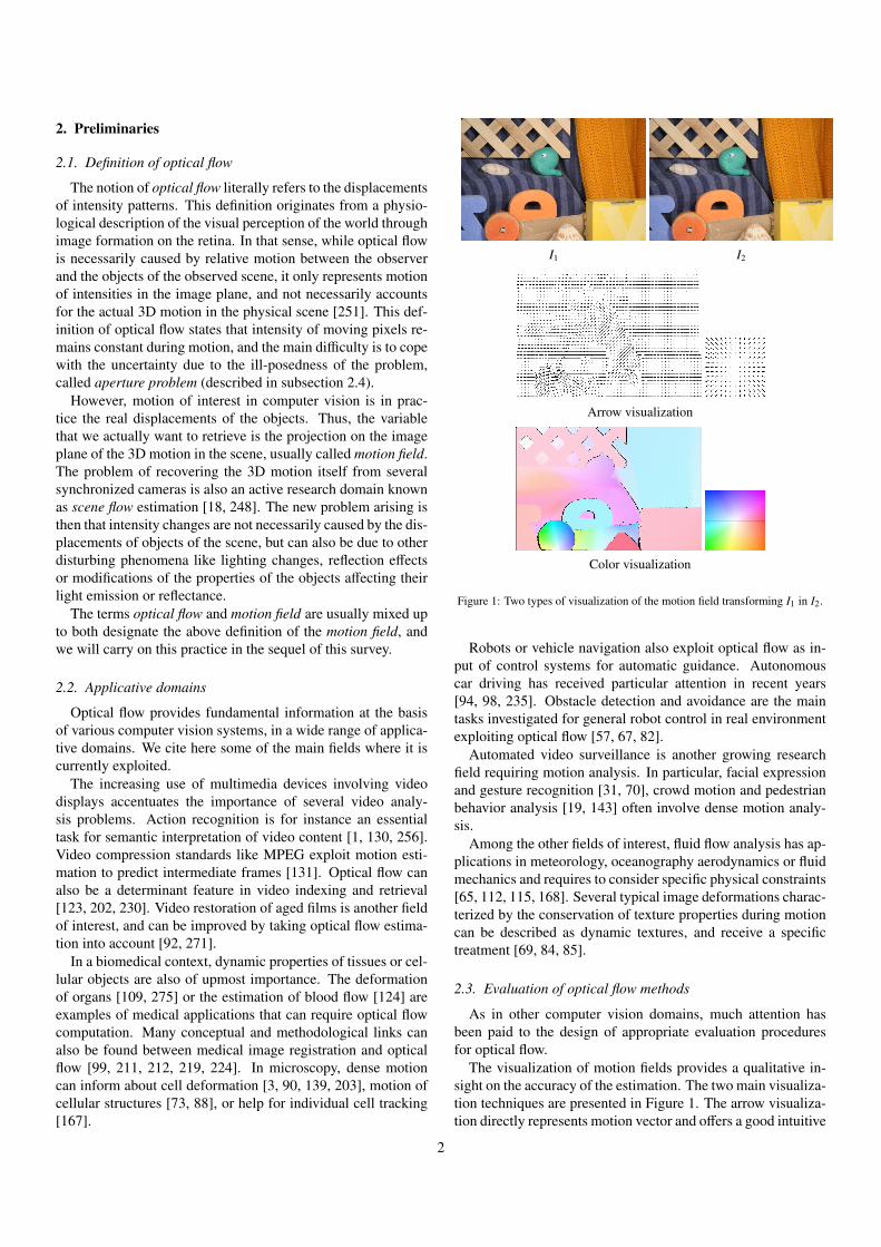
The notion of optical flow literally refers to the displacementsof intensity patterns. This definition originates from a physio-logical description of the visual perception of the world throughimage formation on the retina. In that sense, while optical flowis necessarily caused by relative motion between the observerand the objects of the observed scene, it only represents motionof intensities in the image plane, and not necessarily accountsfor the actual 3D motion in the physical scene [251]. This def-inition of optical flow states that intensity of moving pixels re-mains constant during motion, and the main difficulty is to copewith the uncertainty due to the ill-posedness of the problem,called aperture problem (described in subsection 2.4).

However, motion of interest in computer vision is in prac-tice the real displacements of the objects. Thus, the variablethat we actually want to retrieve is the projection on the imageplane of the 3D motion in the scene, usually called motion field.The problem of recovering the 3D motion itself from severalsynchronized cameras is also an active research domain knownas scene flow estimation [18, 248]. The new problem arising isthen that intensity changes are not necessarily caused by the dis-placements of objects of the scene, but can also be due to otherdisturbing phenomena like lighting changes, reflection effectsor modifications of the properties of the objects affecting theirlight emission or reflectance.

The terms optical flow and motion field are usually mixed upto both designate the above definition of the motion field, andwe will carry on this practice in the sequel of this survey.

2.2. Applicative domains

Optical flow provides fundamental information at the basisof various computer vision systems, in a wide range of applica-tive domains. We cite here some of the main fields where it iscurrently exploited.

The increasing use of multimedia devices involving videodisplays accentuates the importance of several video analy-sis problems. Action recognition is for instance an essentialtask for semantic interpretation of video content [1, 130, 256].Video compression standards like MPEG exploit motion esti-mation to predict intermediate frames [131]. Optical flow canalso be a determinant feature in video indexing and retrieval[123, 202, 230]. Video restoration of aged films is another fieldof interest, and can be improved by taking optical flow estima-tion into account [92, 271].

In a biomedical context, dynamic properties of tissues or cel-lular objects are also of upmost importance. The deformationof organs [109, 275] or the estimation of blood flow [124] areexamples of medical applications that can require optical flowcomputation. Many conceptual and methodological links canalso be found between medical image registration and opticalflow [99, 211, 212, 219, 224]. In microscopy, dense motioncan inform about cell deformation [3, 90, 139, 203], motion ofcellular structures [73, 88], or help for individual cell tracking[167].

I1 I2

Arrow visualization

Color visualization

Figure 1: Two types of visualization of the motion field transforming I1 in I2.

Robots or vehicle navigation also exploit optical flow as in-put of control systems for automatic guidance. Autonomouscar driving has received particular attention in recent years[94, 98, 235]. Obstacle detection and avoidance are the maintasks investigated for general robot control in real environmentexploiting optical flow [57, 67, 82].

Automated video surveillance is another growing researchfield requiring motion analysis. In particular, facial expressionand gesture recognition [31, 70], crowd motion and pedestrianbehavior analysis [19, 143] often involve dense motion analy-sis.

Among the other fields of interest, fluid flow analysis has ap-plications in meteorology, oceanography aerodynamics or fluidmechanics and requires to consider specific physical constraints[65, 112, 115, 168]. Several typical image deformations charac-terized by the conservation of texture properties during motioncan be described as dynamic textures, and receive a specifictreatment [69, 84, 85].

2.3. Evaluation of optical flow methods

As in other computer vision domains, much attention hasbeen paid to the design of appropriate evaluation proceduresfor optical flow.

The visualization of motion fields provides a qualitative in-sight on the accuracy of the estimation. The two main visualiza-tion techniques are presented in Figure 1. The arrow visualiza-tion directly represents motion vector and offers a good intuitive

2

Barron et al. [17]

Middlebury [12]

Kitti [94]

MPI Sintel [52]

Figure 2: Examples of frames and groud truth from the main optical flow evaluation benchmarks.

3

perception of physical motion. On the counterpart, a clean dis-play requires to under-sample the motion field to prevent over-lapping of arrows. The color code visualization associates acolor hue to a direction and a saturation to the magnitude of thevector. It allows for a dense visualization of the flow field and abetter visual perception of subtle differences between neighbormotion vectors.

On the other hand, objective quantitative evaluation basedon error metrics is necessary for an accurate comparison ofmethod performances. When ground truth is available, two er-ror measures are commonly used, namely the Angular Error(AE) and the Endpoint Error (EPE). The AE of an estimatedmotion vector west = (uest, vest)> w.r.t. the reference vectorwre f = (ure f , vre f )> is defined by the 3D angle created by theextended vectors (uest, vest, 1)> and (ure f , vre f , 1)>:

AE = cos−1

uesture f + vestvre f + 1√u2

est + v2est + 1

√u2

re f + v2re f + 1

. (1)

The EPE is defined as the Euclidean distance between the twovectors:

EPE =

√(uest − ure f )2 + (vest − vre f )2. (2)

These two metrics are complementary regarding motion mag-nitude. AE is very sensitive to small estimation errors, occur-ring for small displacement, whereas EPE hardly discriminatesbetween close motion vectors. On the contrary, AE tends tounder-evaluate distances between motion vectors in some casesof large motion magnitudes, while EPE strongly penalizes largeestimation errors.

The design of challenging benchmarks with ground truth onwhich to apply these error measures has motivated a substan-tial amount of work, which main steps are illustrated in Figure2. The first optical flow benchmark with ground truth estab-lished by [17] dealt either with simple parametric transforma-tions applied to real images, like translation or rotation, or withsynthetic sequences for which the true motion is available byconstruction. The resulting motion fields were characterized bysmall displacements and absence of discontinuities. More re-cent benchmarks have been designed to address new types ofproblems or specific applicative issues. The Middlebury bench-mark1 [12, 13] is composed of more challenging sequences,partly made of smooth deformations similar to the sequencesdescribed in [17], but also involving motion discontinuities andmotion details. While some sequences are synthetic, severalothers were acquired in a strictly controlled environment allow-ing to produce ground truth for real scenes. Issues raised byMiddlebury being almost solved by modern methods, the MPISintel benchmark2 [52] has been recently proposed. It is ex-tracted from a synthetic movie and opens new issues mostlyrelated to very large displacements, occlusions, illumination

1http://vision.middlebury.edu/flow/eval/2http://sintel.is.tue.mpg.de/

changes, and effects like blur or defocus. In parallel, dedi-cated datasets have been designed to solve specific problemsrelated to applicative contexts, the most successful example be-ing the KITTI benchmark3 [94] devoted to assisted driving ap-plications.

2.4. Estimation principles

Let us denote an image sequence by I : Ω × T → R, whereΩ ⊂ R2 is the image domain and T is the sampled time intervalof the sequence. Every optical flow estimation method is basedon an assumption on the relationship between the searched mo-tion field w : Ω → R2 at time t and the image I(·, t). The mostnatural and widely used assumption is that pixel intensity re-mains constant during displacement. The brightness constancyconstraint equation (BCCE) is then defined by:

dIdt

(x(t), t) = 0. (3)

Other feature constancy can be chosen, each encoding specificimage properties, which will be discussed in Section 3. Thediscrete approximation of (3) at a given pixel x ∈ Ω and time tyields:

I(x + w(x), t + 1) − I(x, t) = 0. (4)

However, constraint (4) usually generates particularly difficultoptimization problems. It can be much more tractable to con-sider the expanded version of (3) with partial derivatives, result-ing in a linear version of (4):

∂I∂x1

(x) u(x) +∂I∂x2

(x) v(x) +∂I∂t

(x) = 0, (5)

where w(x) = (u(x), v(x))> and x = (x1, x2)>. For the sake ofclarity, we have dropped the dependency of I over t. We canalso write (5) as

∇I(x) · w(x) + It(x) = 0, (6)

where ∇· =(∂·∂x1, ∂·∂x2

)Tis the spatial gradient operator, It =

∂I/∂t is the partial temporal derivative and the dot ” · ” denotesthe inner product.

The linearized brightness constancy constraint (5) providesonly one equation to recover the two unknown components ofw(x). From this single constraint, the component of the mo-tion vector w(x) in the direction of the image gradient can becomputed, but the two-dimensional problem remains under-constrained. This is known as the aperture problem, stating thatmotion of linear structures, as it is assumed by (5), is by natureambiguous if the neighboring context is not taken into account.

To make the problem well-posed, it is necessary to introducean additional constraint encoding a priori information on w.The a priori will take the form of spatial coherency imposedby either local or global constraints, described in Section 4 andSection 5.

3http://www.cvlibs.net/datasets/kitti/index.php

4

It is important to mention that while (4) holds for motion ofarbitrary magnitude, the continuous motion constraint (5) re-stricts its validity domain to the linear region of I, which usu-ally corresponds to small displacements or very smooth im-ages. The linearization is nevertheless necessary for methodsrelying on differential computations. The standard techniqueto cope with large displacements is to embed the estimation ina coarse-to-fine scheme [27, 81, 174]. The idea is to create apyramid of coarse-to-fine downsampled versions of the origi-nal image. At the coarsest level, the linearity domain of theimage encompasses large displacements and the estimation canbe based on (5). The estimations at coarser levels serves towarp the image at subsequent finer levels, where the estimationthen reduces to a search for small motion increments. The so-lution is iteratively refined at each level until reaching the fullimage resolution. It is possible to continue the process in stillhigher resolutions created by interpolation, as proposed in thecoarse-to-overfine approach [5]. The solution at each level ofthe multi-resolution pyramid can be interpreted as a fixed pointin the direct optimization of the non-linearized constancy equa-tion (4) [46]. Almost all differential methods concerned withlarge displacements resort to the multiscale approach, possiblywith some additional strategies to avoid its drawbacks.

The main undesirable effect produced by smoothing at coarselevels is the loss of small and rapidly moving objects in the finalestimated flow field. If the object extent is smaller than its dis-placement, it is likely to be smoothed out at coarse levels andthen “forgotten”. Avoiding this drawback has been a very activetopic in recent years. It has been accomplished mainly by in-tegrating feature matching in the estimation process, as will bediscussed in Section 7, or by resorting to discrete optimizationmethods, as detailed in Section 5.2.2.

3. Data cost

The deviations from the data constancy assumption (3)are penalized at every pixel x ∈ Ω via a data potentialρdata(x, I1, I2,w), defined in the case of brightness constancy (4)as

ρdata(x, I1, I2,w) = φ(I2(x + w(x)) − I1(x)), (7)where I1 = I(·, t) and I2 = I(·, t + 1) denote two successiveframes, and φ(·) is the penalty function.

The brightness constancy assumption is in practice an imper-fect photometric expression of the real physical motion in thescene. A common counter-example consists in moving the lightsource of an immobile scene, producing brightness variationswithout motion of any objects. In general, while it is possibleto create synthetic sequences for which the constraint strictlyholds [52], it is often violated in practice in case of changesin the illumination sources of the scene, shadows, noise in theacquisition process, specular reflections or large and complexdeformation.

Choosing a quadratic penalty function φ(z) = z2, as in earlyworks [120, 170], makes optimization much easier, but assumesthat the residual of the brightness constancy constraint equa-tion (3) is normally distributed and thus gives a strong influ-ence to large localized violations mentioned above. It is then

common to resort to robust statistics [125] to reduce the impactof local errors considered as outliers. Common robust alterna-tives to quadratic penalty are the L1 norm [46], the Tukey func-tion [193], the Lorentzian norm [27] or the Leclerc’s function[174]. Adapted optimization schemes must then be adopted tocope with non-linearity or non-convexity induced by the robustterms, as will be discussed in Sections 4.2 and 5.2. A priorismoothness assumption based on parametric constraint (Section4) or explicit regularization (Section 5) also counterbalances lo-cal invalidity of data constancy.

Robust statistics and regularization treat the problem of vio-lations of the constancy assumption by considering it as noise,with underlying distribution assumptions [155, 221]. The con-sidered distributions may not suitably model the possibly largelocalized violations implied by the above listed causes. There-fore, a large number of alternatives to brightness constancy havebeen proposed, aiming at more stable invariance properties. Afew experimental studies have compared performances of dif-ferent data costs given fixed optimization and regularizationcontexts [227, 252].

Let us notice as a preamble to this section that it is difficultin practice to design a data term independently from the spa-tial coherence constraint and the optimization strategy to whichit will be associated. For example, sophisticated feature con-servation usually involves specific optimization difficulties, andthus requires careful design of the optimization solution. Wewill dedicate this section to a review of the main classes of dataterms for optical flow estimation, emphasizing their validity do-mains and their limitations, independently from the estimationcontext in which they were elaborated.

3.1. Beyond brightness constancyWe explore several matching costs aiming at overcoming the

drawback of the brightness constancy, in particular its sensitiv-ity to noise and illumination changes.

3.1.1. Image transformationA first class of data potentials exploits the same pixel-wise

form as (7), but operates on a tranformed version f (I) of theoriginal image sequence:

ρdata(x, I1, I2,w) = φ( f (I2)(x + w(x)) − f (I1)(x)) (8)

Image smoothing. We can first notice that Gaussian smoothingis applied as a pre-processing step by most methods [46, 286],in order to reduce the influence of noise. It can be viewed as amodified version of brightness constancy, setting f as a Gaus-sian filtering operator.

High-order constancy. Image derivatives possess illuminationinvariance properties that are well suited for motion estimation.The constancy of spatial image gradient, defined by f (I) = ∇I,has been introduced in [245] for its ability to overcome theaperture problem when the determinant of the Hessian is non-zero. However, when applied on the directional derivative vec-tors, the gradient conservation only holds for translational or di-vergence motions. To achieve rotational invariance, the penalty

5

should rather be applied on the magnitude of the derivatives,that is f (I) = ‖∇I‖ [46]. It was subsequently used in the con-text of the local approach (see Section 4) in [240] and integratedin global variational methods (see Section 5) in [46].

Despite a demonstrated performance gain in the case of ad-ditive illumination changes compared to brightness constancy,gradient information is also much more sensitive to noise, anddisappears in poorly textured regions. Therefore, it is alwaysused in addition to brightness constancy. A large number ofmethods rely on this combination and achieve good results[46, 181, 279]. Finally [198] investigated higher-order dataconstancy like Laplacian of the image f (I) = ∆I, or norm anddeterminant of the Hessian f (I) = |H I|, f (I) = det(H I).

Texture. Another way to obtain robustness against illumina-tion changes is to work with the cartoon and texture compo-nents of the image, as initiated in [263]. The decompositionproposed in [8] consists in first obtaining the structure part IS

by discontinuity-preserving smoothing (using the ROF model[210] in [263]), and then deriving texture part IT by subtractingIS to the original image. Additive illumination changes only af-fect the cartoon image while the texture image is less impacted.However, even if IT captures most image information, it is stillinsufficiently discriminative in some regions, and it is also moresensitive to noise than IS . To limit this drawback, the textureimage used to compute optical flow is usually blended with thecartoon part by a parameter γ [154, 232, 262]: f (I) = IT − γIS .

Colour spaces. When dealing with colour images, severalphotometric-invariant colour spaces can be exploited. Inparticular, multiplicative illumination invariance is essentialfor realistic illumination models [246] and is achieved in theHSV space by the hue channel (local and global changes) andthe saturation channel (only global changes) [176]. As forpreviously mentioned image transformations, the benefit inillumination change regions coincide with a loss of informationin other parts, and the colour channels are in practice combinedwith the intensity valued channel [286]. Other colour spaceslike normalized RGB [103] or spherical space [246] have beeninvestigated.

Combination of linear filters. As mentioned before, it is of-ten necessary to combine several constancy assumptions. It hasbeen achieved in [259] by considering K different linear filtersfk providing a system of constancy equations to be solved ateach pixel. In [231], a learning approach is proposed for find-ing the best combination of constraints. The data constraintsinduced by the linear filters fk are imposed through a GaussianScale Mixture (GSM) φGS M .

ρdata(x, I1, I2,w) =

K∑k=1

φGS M( fk ∗ I2(x + w(x)) − fk ∗ I1(x),Ξk),

(9)where ∗ denotes the convolution operator and Ξk are the pa-rameters of the GSM associated to each filter. By learning the

parameters of the GSM from a set of ground truth sequences,the “weights” of each filter in (9) are automatically determined.These weights are constant in the whole image. Spatially adap-tive combination is also of upmost importance and will be ad-dressed in Section 3.2.1.

3.1.2. Patch-based similarity measuresRather than pre-filtering images, neighborhood information

can be integrated directly in the data term by patch-based simi-larity measures. Let us point out that a major issue with patch-based measure is the determination of the size an possibly shapeof the patch.

Filtering the data term. In addition to pre-smoothing the im-ages (8), Bruhn et al. [50] proposed to filter the data potentialas follows:

ρ(x, I1, I2,w) = f (φ(I2(x + w(x)) − I1(x))) , (10)

where f is chosen as a Gaussian filter. While it was demon-strated beneficial for very noisy sequences, this choice also sig-nificantly blurs motion discontinuities and degrades the overallperformance for low amount of noise, compared to pixel-wisedata term, as emphasized in [286]. This limitation is addressedin [78, 206] by replacing the Gaussian filtering with anisotropicdiscontinuity-preserving filtering (e.g. bilateral filtering in [78]and tensor voting in [206]). The relation between adaptive fil-tering and non-linear diffusion has also been exploited in [48].

Correlation-based measures. Similarity measures based oncross-correlation have been extensively used for various cor-respondence problems [44]. Normalized Cross Correlation(NCC) is usually preferred for its invariance to linear illumi-nation changes. The NCC for a windowW(x) centered at pixelx is defined as

NCC(x, I1, I2,w) =∑y∈W(x)(I2(y + w(x)) − µ2(x + w(x)))(I1(y) − µ1(x))

υ1(x)υ2(x + w(x))(11)

where for i = 1, 2, µi(x) is the mean and υi(x) the standard de-viation of Ii in the windowW(x). The associated data potentialis

ρdata(x, I1, I2,w) = 1 − NCC(x, I1, I2,w). (12)

NCC is actually discriminative enough to be used in a match-ing procedure without additional regularization, and producescoarse but reasonably robust motion fields. It is used in severalapplications like stereovision [72], fluid flow analysis [22] orbiological imaging [146] where it also enables direct physicalmeasures for diffusion processes.

The computational cost of (11) is a major limitation. Un-like simple cross-correlation which can be efficiently computedwith Fast Fourier Transform (FFT), the computation of NCC formatching purpose cannot be easily performed in the frequencydomain. In [163] only the numerator is computed with FFT andthe denominator is rewritten as a product of sums, independentof the position of the pixel and thus efficiently computable with

6

integral images [83]. In [171] this idea is generalized and thenumerator is also computed with integral images, dramaticallyreducing the computation time and making it invariant to thepatch size.

The challenge of integrating NCC in a variational opti-mization scheme is to cope with its non-differentiability.Indeed, Taylor expansion on the terms containing w(x) in(11) still yields a highly non-linear potential. The approachof [180, 272] has been applied to NCC but is able to handlearbitrary data terms as well. The authors directly linearizethe data term and compute its spatial derivatives with finitedifferences. Werlberger et al. [272] keeps a second-orderapproximation to ensure the convexity of the energy, necessaryin the primal-dual scheme used. Another recent techniqueallowing fast computation of NCC relies on the fact thatNCC is actually equivalent to the Sum of Square Differences(SSD) when the images are filtered with the cheaply computedcorrelation transform [79].

Census. Census transform [283] recently regained inter-est and was promoted in [226] for optical flow estimation[108, 118, 179, 182, 183, 205, 252]. The Census signature isa bit string reflecting relative value of pixels of a patch withrespect to the center pixel. By discarding the absolute intensityvalues, only the structure of the neighborhood is encoded inthe signature, which makes it robust to illumination changes.It has shown robust behaviour in outdoor scenes and vehicledriving scenarios [205, 226, 252]. Integrating the Censustransform in variational optical flow is not trivial since it cannotbe easily linearized. Solutions to remedy this problem areconvex approximation [252], reformulation as a generalizationof the gradient constancy conservation [108] or linearization ofthe data term [182, 205] as previously mentioned for NCC [272]

3.2. Spatially adaptive data cost

The validity of each of matching costs is limited to a givenrange of visual situations. In a single frame, regions can coex-ist satisfying a given constancy assumption, and violating oth-ers. One solution could be to linearly combine them to takeadvantage of their complementary invariance properties. Softlyselecting the best constancy constraint at each pixel is usuallydevoted to the robust penalty function, limiting the influenceof local constraint violations. However, the data term shouldideally be spatially adapted.

We distinguish two classes of methods achieving the spatialadaptivity: i) optimization of the weights of a linear combi-nation of data potentials, and ii) estimation of the spatial dis-tribution of the errors attached to a single data potential. Thenormalization of the data term used in [214, 221, 286] couldfall in this category since a spatially varying weight is appliedto the data term. It is derived from the linearized brightnessconstancy equation to prevent too strong constraints in regionsof high image gradient (see a detailed interpretation in [286]).

3.2.1. Combination of constancy assumptionsThe combination of P data constraints can be expressed as

the weighted sum of their associated potentials ρp(x, I1, I2,w):

ρdata(x, I1, I2,w) =

P∑p=1

λp(x) ρp(x, I1, I2,w). (13)

Weights λp(x) are spatially variant and have to be optimized tolocally favor different data terms.

The idea of combining several data constraints has alreadybeen explored twenty years ago in [116]. In addition to theclassical brightness constancy, the authors exploited a comple-mentary sparse edge-based constraint. Weights λp(x) are binaryconfidence measures derived from hypothesis testing providingevidence on each constraint.

In [279], intensity and gradient conservation are combinedand their complementarity is experimentally demonstrated. Theweights are defined to operate a binary selection between thetwo constraints and are obtained by considering a mean field ap-proximation of (13), which intuitively amounts to selecting theconstraint having the lower (normalized) potential. This ideahas been used subsequently in [181].

The work of [140] addresses the problem in its most generalform (13), allowing the combination of an arbitrary number andtype of data conservation assumptions. A confidence measurefor arbitrary data term is designed as an extension of the featurediscriminability [218] to data discriminability. The confidencemeasures are used as local constraints on the weights λp(x) in(13), and a regularization on λp(x) is also imposed. The weightsare then optimized jointly with the motion field.

3.2.2. Modeling intensity variationsAnother way to handle errors related to the constancy con-

straint is to design more elaborated models of intensity vari-ations. The goal is to explicitly model the intensity changesdue to environmental effects so as to isolate more accuratelymotion-induced changes.

The most common approach introduces an additional vari-able representing deviations from constancy assumption by afunction e(x, I1, I2, ξ) parametrized by the vector ξ:

ρdata(x, I1, I2,w, ξ) = φ(I2(x+w(x))−I1(x)−e(x, I1, I2, ξ)). (14)

The model proposed by [188] is composed of an offset changeξo : Ω → R, accounting, e.g., for moving shadows or high-lights, and a multiplicative change ξm : Ω → R encoding lin-ear illumination variations. The error function can then be ex-pressed as

e(x, I1, I2, ξ) = ξm(x)I1(x) + ξo(x). (15)

This general formulation has been exploited in a number ofworks, considering either the offset parameter alone [55, 88,193], the multiplier alone [285] or both parameters [142, 159,239]. They may differ on the type of spatial coherency, thepenalty function, or the optimization strategy. A smoothnessconstraint is assumed on ξo and ξm, either with a local para-metric form [188, 193] or a global regularization [55, 88, 142,

7

159, 239]. The offset formulation is also used in [10, 89], butis associated to a sparsity constraint aiming at retrieving vio-lations due to occlusions. The more general approach of [74]parametrizes intensity changes in terms of Brightness Trans-fer Function [106], which coefficients are learned from trainingdata.

The model (15) is based on a general polynomial approxima-tion. If specific knowledge about the observed physical processis available, dedicated models can be designed. A number ofphysical constraints are explored in [110], where a generic localestimation framework is designed based on a Taylor expansionof arbitrary data constraints similar to the subsequent methods[180, 272].

4. Parametric approach

As explained in Section 2.4, a spatial coherence constrainton the flow field must be added to the previously describeddata terms. To this end, one can impose the flow field to fol-low a parametric model in region R ⊆ Ω. The motion fieldwα : R → R2 is then fully characterized by the associated pa-rameter vector α. When the region R is a small sub-domain ofthe image, these methods are referred to as local approaches.The objective energy to be minimized is the weighted sum ofthe potentials provided by each pixel of R:

α = arg minα

∑x∈R

g(x) ρdata(x, I1, I2,wα) (16)

where g(x) is a spatial weighting function controlling the influ-ence of pixel x in the estimation.

It is crucial to determine the local estimation domain wherethe parametric form of the motion model is a valid approxima-tion of the true motion. Low-order polynomial motion mod-els like translation or affine deformation can usually representmotion in small neighborhoods, whereas more complex modelslike deviations from affine constraint or combination of basisfunctions can deal with larger regions.

We first give an overview of the mostly used motion mod-els and their associated optimization strategies. Secondly, wediscuss about the different ways to define appropriate local es-timation supports.

4.1. Motion models

The choice of the motion model is driven by a trade-off be-tween efficiency and representativeness. Complex nonlinearand physical-based models can be exploited to model defor-mations for image registration [224]. These models are partic-ularly well adapted to physically constrained situations as theycan be encountered in medical imaging, and in particular to cap-ture smooth deformations. In contrast, optical flow is dealingwith temporal sequences of arbitrary content, usually involvingmotions of several objects with unrelated behaviours, generat-ing motion discontinuities as well as smooth motion parts. Asa result, it is difficult to capture the whole complexity of mo-tion fields with a single unifying and computationally tractableparametric model. Therefore, attempts in this direction are not

frequent and not among the best performing methods in opticalflow benchmarks. The approach of most parametric methodsfor optical flow is rather to rely on much simpler motion mod-els, mostly polynomial models, and to restrict their applicationto local domains, where they can represent accurate approxima-tions.

We will restrict ourselves to linear models of the form

wα(x) =

K∑k=1

bk(x)αk(x), (17)

where b = bk(x)k∈[1,K], bk(x) ∈ R2 are basis functionsand α(x) = αk(x)k∈[1,K] are the parameters to be optimized.Other parametric models than those described here can befound, like planar surfaces or rigid body [23], or waveletbases [75, 76, 217, 274]. It can also be noted that parametricmodels are sometimes completed with explicit regularizationterms (see Section 5) imposed on the parameters themselves[75, 133, 175, 191].

4.1.1. Polynomial modelsPolynomial models are among the most compact parametric

representations of motion fields and are also remarkably wellsuited to retrieve local physical motion of individual objects andeven deformable motion. The polynomial model can be seen asa special case of (17), which we write for clarity as:

wθ(x) = B(x) θ, (18)

where B(x) is a matrix determining the form of the model andθ is the parameter vector. Apart from the exception of [191]where the parameters are spatially variant and regularized, theparameter θ is kept constant over the estimation domain. Thematrix B(x) depends on the pixel coordinates x ∈ R, and the or-der of the polynomial determines the complexity of the motionfield. Low-order polynomials are usually sufficient to modelsmooth motion fields, and their small number of parameters al-lows for efficient computation. The two mostly used polyno-mial models correspond to the translation and the affine motion:

Translational : θ = (a1, a2)>; B(x) =

(1 00 1

)Affine : θ = (a1, a2, a3, a4, a5, a6)>;

B(x) =

(1 x1 x2 0 0 00 0 0 1 x1 x2

)with x = (x1, x2)>.

The translation assumption is very restrictive and must beapplied to very small regions [170]. The physical assumptionunderlying the affine model is a rigid motion of 3D planar sur-faces projected orthogonally on the image plane. Higher-orderpolynomials can model more complex situations, but are stilltoo smooth to allow for motion discontinuities. For example,the 8-parameter quadratic model represents rigid motion of aplanar surface in perspective projection. The small number ofparameters of the affine model and its realistic local assumptionmake it often considered as the best trade-off between complex-ity and descriptiveness [27, 89, 175, 193]. The accuracy of of

8

local affine motion estimation in appropriate estimation supportwas experimentally demonstrated in [89].

4.1.2. Learned basisThe basis functions can also be learned from a set of train-

ing flow fields. As for polynomial models, the resulting learnedmotion models cannot describe motion of complex scenes, butthey are able to retrieve a larger diversity of local motion pat-terns, including discontinuities.

The design of the training set reflects the assumption on theform of the flow. In a generic point of view, Black et al. [32]used synthetic motion fields representing simple motion pat-terns. The method of [190] relies on a large number of patchesof ground truth motion fields. The training set can be dedi-cated to a specific application, as in [87] where the aim is toestimate mouth motion. To avoid resorting to external groundtruth, [93] defines the training set on the processed sequenceitself. The basis set is composed of trajectories constructed byfeature tracking on large temporal scales, in regions ensuringreliable tracks. In all these works, an orthogonal basis of flowfields is generated by PCA decomposition, conserving only thefirst K components containing most of the variance of the train-ing set.

4.1.3. Free-form deformationsThe free-form deformation model (FFD) [211] has been orig-

inally introduced for image registration and has demonstratedgreat efficiency to retrieve smooth deformations. The displace-ments are defined on a coarse regular subgrid of the image andis interpolated on the final resolution with B-splines. The mo-tion basis bk(x) is thus formed with the displacements of theK control points and coefficients αk(x) are B-spline influencefunctions. The dimensionality reduction induced by the sub-sampling of the image grid makes the computation much easier,and the spatial coherence of the deformation is ensured by theB-spline interpolation. On the counterpart, the framework can-not retrieve sharp motion discontinuities, while it is necessaryfor optical flow applications. Image-adaptive non-regular con-trol points distribution [212] or coarse-to-fine spacing strategies[211] are possibilities to address this issue.

The work of [236] was the first to apply this idea to opti-cal flow, with non-uniform control points defined on image-driven quadtrees. In [201], B-Splines defined on a uniform gridare used to retrieve smooth deformations. In [100] the prob-lem is turned in a discrete setting. The range of motion labelsis iteratively adapted by estimating a local uncertainty covari-ance. Despite good results, the method is still limited by over-smoothing. The method of [219] addresses the discontinuityproblem with a sparsity constraint on the B-spline coefficients,allowing to modulate the influence of the control points. Recentapproaches [99, 100, 219] also add an explicit regularization onthe motion field, overlapping with the methodology describedin Section 5.

4.2. OptimizationParametric models are usually associated with the penalty of

a pixel-wise data constancy constraint (7). In case of intensity

constancy (5), energy (16) then writes:

E(α) =∑x∈R

g(x)φ (∇I(x) · wα(x) + It(x)) (19)

where ∇I is the image gradient and It = ∂I/∂t. The specialcase of a quadratic function φ and a translational model as in[170] leads to a very simple optimization problem, since thecancelling of the derivatives of (19) amounts to solving the lin-ear system Mα = b, with

M =

( ∑x g(x) I2

x1(x)

∑x g(x) Ix1 (x)Ix2 (x)∑

x g(x) Ix1 (x)Ix2 (x)∑

x g(x) I2x2

(x)

)b = −

( ∑x g(x) Ix1 (x)It(x)∑x g(x) Ix2 (x)It(x)

)where Ix1 and Ix2 are the partial derivatives of I respectivelyalong the horizontal axis x1 and the vertical axis x2. The rankof M allows one to decide if a unique solution of the linearsystem exists, and can be used to adapt the size of the localdomain R (see Section 4.3.2). Despite the limitations of thequadratic penalty, this approach has become very popular for itsimplementation simplicity, low computational cost and avail-able code in the OpenCV library [36, 41].

However, robust estimation is often advocated [27, 32, 76,193, 215] as mentioned in Section 3, especially for polyno-mial models, to deal with the frequent case of multiple motionsin the estimation domain. Among the variety of optimizationmethods used in case of robust penalty function, the IterativeReweighted Least Squares (IRLS) [119] and gradient descentapproaches have mostly been used. IRLS proceeds by succes-sive optimizations of quadratic problems weighted by a func-tion of the current estimate and is implemented in the Motion2Dsoftware [193, 215] with . Gradient descent approaches are of-ten coupled with Graduated Non-Convexity (GNC) [27, 33] tocope with non-convexity of (19). Regarding the slow conver-gence of steepest descent, it is preferable to use second orderapproximations and Newton methods, or quasi Newton meth-ods like L-BFGS or Levenberg-Marquardt, approximating theHessian for large dimension problems.

4.3. Neighborhood selection

As previously mentioned, the spatial adaptation of the param-eters α(x) is a way to cope with complex and discontinuous flowfields [93, 191, 219]. This approach often involves a priori con-straints on the spatial distribution of α(x) and is thus stronglyrelated to the methods that will be presented in Section 5. Sucha dense parameter map moves away from the compactness ofparametric models.

On the other hand, when parameters are constant over theestimation domain R, the resulting motion field is smooth andcan constitute a valid approximation only in regions of coherentmotion. The region R must be large enough to enable motionestimation, while small enough to keep valid the parametric ap-proximation (generalized aperture problem [27]). We will de-scribe below the strategies for defining R in the case of constantparameters α(x) = α over R, for polynomial models.

9

4.3.1. Entire domainDespite their inability to retrieve realistic motion in arbitrary

scenes, polynomial models combined with robust estimationare well adapted to capture the dominant image motion. Ap-plied in the whole image domain Ω, they become particularlyuseful to separate or compensate the camera motion [193]. Ap-plications to moving object detection [194] or to action recog-nition [202] are among the most common ones.

4.3.2. Square patchesThe approach initiated by [170] performs independent esti-

mations in small square or circular patches. Most of the relatedmethods use fixed patch size, and conserve the velocity vectordeduced from the estimated motion model at the square center[11, 26, 141, 285]. This choice is very popular for its simplicityof implementation and can be naturally parallelized [222, 285].It is still extensively used for numerous applications. However,following the generalized aperture problem, patches centered ateach pixel with a fixed size are likely to contain either multiplemotions or no image gradient.

Multiple motions in a single patch can be partially handledwith robust estimation by rejecting secondary motions, consid-ered as outliers [27, 95, 193, 215].

The second option is to adapt the size or the position of thepatch so that it contains an unimodal motion distribution. Thesize of the patch can be adapted with a bias-variance criterion[173], or based on a confidence measure on the reliability of thelocal domain for parametric estimation. Starting from a smallpatch size, it is thus possible to increase the size of the patchuntil the condition for a reliable domain is violated [173, 215].In the translational model case, one can analyze the singular-ity of the matrix M of the linear system (20) and, for example,impose a minimum threshold to the maximum eigenvalue of M[17]. Rather than adapting the size, [132] adapts the position ofthe patches. Patches corrupted by strong intensity edges are dis-placed by a mean-shift procedure to reach more homogeneousregions. The method described in [89] adapts both size andposition of the square patches. This adaptation is performedthanks to the aggregation framework decoupling the estimationof candidates with predefined sizes and positions, and their se-lection achieved with a global model (see Section 5).

Finally, local adaptation of the weights g(x) in (16) is anotherway to adapt the estimation support. It can be done for instancewith bilateral filter weights as in [78], or using the non-linearstructure tensor [48].

4.3.3. Segmented regionsThe optimal supports to perform polynomial motion estima-

tion ideally correspond to a segmentation of the image in co-herently moving regions. We briefly describe two types of ap-proaches: independent image segmentation and joint estimationof motion and region supports or frontiers.

Image segmentation. While the ultimate goal is to segment theunknown motion field, color-based image segmentation is amuch simpler alternative which can help motion estimation. It

can be reasonably assumed that motion discontinuities coincidewith image discontinuities (but the inverse is far from beingtrue). It implies that an image segmentation is a motion fieldover-segmentation, and obtained regions are thus guaranteed tocontain no motion discontinuity. However, merely estimatingmotion in the resulting regions is problematic for two reasons.

The first limitation is that the segmented regions may notcontain enough information for motion estimation. Paramet-ric estimations in these regions must be performed by circum-vented ways. The very fine over-segmentation of [287] imposesfor instance to perform region matching. Generally, an inde-pendent coarse and cheap motion estimation is fused with thecolor image segmentation to overcome the lack of information[28, 34, 278]. In [278], hybrid regions are found by apply-ing mean-shift segmentation in the extended space of color andmotion. Differently, [28, 34] fit a parametric flow field on thecoarse initial motion field, obtained with a global regularizedmethod [30] for [28], and with the sparse KLT tracker [218] for[34].

The second problem is that spatial coherence between esti-mated motion in neighboring segments is not ensured. Globalregularization (see Section 5) can here be imposed, either on themotion parameters associated to each region [278] (similarlyto [133], not resorting to image segmentation), on the coarsemotion field completing color information [28] or, in a layeredapproach, on the layer assignment function [34]

Joint estimation and segmentation. Color segmentation is usu-ally too dependent on the image content to make it the basis of arobust motion estimation method. Rather than considering seg-mentation and estimation as two independent tasks, most meth-ods have a coupled approach of the problem. Motion param-eters and region supports are jointly estimated by minimizinga global energy imposing a coupling between them. This ap-proach has first been addressed as a labelling problem [37, 195]where the label field l : Ω → l1, . . . , lN associated to the Nregions is estimated jointly with the motion parameters in eachregion α = α1, . . . , αN, in a discrete Markov Random Fieldframework:

E(α, l) =∑x∈Ωd

ρdata

(x, I1, I2,wαl(x)

)+

∑<x,y>

ρMRFreg (l(x), l(y)), (20)

where Ωd is the discrete image domain and ρMRFreg (l(x), l(y)) is

a regularization prior on the label field, typically chosen asρMRF

reg (l(x), l(y)) = 1 − δ(l(x), l(y)), with δ(·) the Kronecker func-tion. The optimization is done alternatively between motionand regions. Another viewpoint in a variational framework ex-tends the Mumford-Shah formulation of image segmentation[184] to motion segmentation [66, 199, 247]. In addition to thedata fitting potential inside each region Ri, a constraint restrict-ing the lengthL(C) of the set of region boundaries C is imposedglobally, resulting in the energy

E(α,C) =

N∑i=1

∫Ri

ρdata(x, I1, I2,wαi )dx + νL(C). (21)

10

The minimization is performed alternatively on the flow and theboundaries. Minimizing (21) with respect to C requires a differ-entiable approximation of the contour length L(C). It is com-mon to implicitly represent the partitioning of the image withlevel sets, which allows to represent the interior of the regionsby the sign of the function, as well as the total length of theboundaries by their level lines. One level set function can onlyrepresent two regions. For an arbitrary number of N regions, itis possible to define N corresponding levels sets, at the price of ahigh computational cost and a more complex energy to preventvacuums in the partitioning. Other strategies can be employed,as the one of [56] re-used in [66], for more sophisticated com-binations between functions. In [199], this level set frameworkis augmented with an edge-driven tracking and background de-tection. In [207], the two images are jointly segmented, andthey influence each other through a dynamic prior term deter-mined by the similarity of the two evolving shapes. Segmen-tation of static and dynamic textures is performed in [85] byassigning different data conservation assumptions to each class.A graph-cut optimization scheme has been proposed in [80].These two formulations (20) and (21) can be found in numerousother works [138, 175, 213, 244]. Similarly, layered approaches[9, 223, 232, 234, 257, 276] aim at decomposing the observedscene into overlapping layers and introduce information aboutdepth ordering of regions. An important interest of such meth-ods is to provide a natural occlusion handling framework.

Two main drawbacks affect the joint motion estimation andsegmentation approach. First, alternating minimization w.r.t.regions and flow fields is computationally expensive. The re-lated layered approach [233, 234] achieving state-of-the-art re-sults requires several hours to process a pair of 640×480 pixels,and even GPU-based implementation [244] can need up to anhour.

Second, the initialization of motion and segmentation param-eters usually has a substantial impact on the evolution of the re-gion contours throughout the minimization procedure. There-fore, paradoxically, the best performing methods in terms ofaccuracy of optical flow fields resort to pre-calculated motionfields obtained with independent methods to initialize their al-gorithm. For example, the results reported in [233] and [244]are obtained with an initialization by the result of the meth-ods of [232] and [269] respectively. Nevertheless it is shownin [244] that the initialization affects more the speed of conver-gence than the final result.

Some works exploit more complex flow field representationsthan polynomial approximation, by authorizing deformationsfrom an initial affine model [28, 175, 233] or an explicit regu-larized model [4, 47]. Allowing such complex and discontinu-ous motion fields in segmented regions actually tends too pro-duce larger regions, and ultimately leads to global approacheswhere motion discontinuities are handled by the global mod-eling itself. Consequently, regions may not represent coherentmotion, but rather a delineation adapted to the specific estima-tion method. Finally, imposing prior on shapes and contourshas been investigated in medical imaging [137], but a limitednumber of regions can be handled at the same time.

5. Regularized models

In an alternating manner to the parametric representation ofspatial coherence, mostly adapted to smooth deformations, theglobal form of the motion field can be imposed by an explicitregularization term. Motion discontinuities are then no morerepresented by the boundaries of the regions delimiting para-metric motion fields, but they are involved in the global model,often considered as outliers w.r.t. smoothness assumptions. Thevariational approach has been initially proposed by [120] and isusually referred to as the global approach, since the regulariza-tion term interconnects all the pixels of the image and thus re-quires the optimization of the objective energy to be performedglobally. In this subsection, we review current versions of theregularization model and optimization strategies.

In its most general form, the energy minimized by globalregularization methods can be written as:

Eglobal(w) =

∫Ω

ρdata(x, I1, I2,w) + λ ρreg(x,w)dx (22)

where ρdata(x, I1, I2,w) is the data potential, as discussed in Sec-tion 3, ρreg(x,w) is the regularization potential encoding an apriori assumption on the field w, and λ is a parameter tuning thebalance between the two terms. Broadly speaking, the regular-ization potential aims at smoothing the motion field in regionsof coherent motion while preserving motion discontinuities atthe boundaries of moving objects. Finding the trade-off can alsobe partially addressed in the adaptation of the balance parame-ter λ [113, 156, 189, 286].

A major interest of the global variational framework is itsversatility, allowing one to model different forms of flow fieldsby combining different data and regularization terms. One mustnevertheless keep in mind that minimizing (22) is often a trickytask. The potentially unlimited combinations of data terms andregularization terms is restricted in practice to those compati-ble with efficient minimization. Besides, advances in opticalflow have often been correlated with new possibilities offeredby optimization techniques. For example, efficient Primal-Dualminimization for Total Variation regularization [55] have mo-tivated a number of optical flow models [244, 270, 284]. Thedevelopment of efficient discrete optimization techniques basedon graph cuts [40] or message passing [147] also inspired var-ious works [59, 161, 181]. Another consequence of the closeintricacy between energy model and optimization technique isthe difficulty to compare performances of different models, asglobal optimum is in general not guaranteed for sophisticatedenergies and the quality of the local optimum depends on thetype of optimization method.

We will detail in Section 5.1 existing regularization mod-els independently from optimization techniques, for the sake ofclarity. Section 5.2 focuses on the dependency between specificenergy models and optimization methods.

5.1. Regularization models5.1.1. Spatial flow gradient constraint

The most natural and widely used way to impose smooth-ness of the motion field is to penalize the magnitude of the flow

11

gradient:ρreg(x,w) = h(x, I1) φ(‖∇w(x)‖2) (23)

where φ(·) is the penalty function and h(x, I1) is a weightingfunction.

A taxonomy of optical flow regularizers has been proposedin [264]. The authors focus on convex and rotational invarianceproperties, and prove uniqueness of the solution in each case.For each regularization of type (23), they show the equivalencebetween the resolution of the Euler-Lagrange equations associ-ated with energy (22) and diffusion filtering. In addition, a dif-fusion tensor is derived for each particular variation of (23). Wewill give a more succinct overview, taking only some elementsfrom this classification and integrating more recent approaches.

Flow-driven regularization. In flow-driven approaches, no re-lation between the form of the flow field and the structure ofthe image is assumed. The weighting function is thus h(x, I1) =

1, ∀x ∈ Ω. The seminal formulation of [120] adopts a quadraticpenalization function:

ρreg(x,w) = ∇u(x)2 + ∇v(x)2, (24)

with w(x) = (u(x), v(x))>. The quadratic penalization beingunable to capture motion discontinuities, the introduction of acomplementary line process to handle motion discontinuitiesin the MRF framework [116, 153], and the use of robust sub-quadratic penalties [27, 77, 174] have soon been employed toovercome the problem. Among the wide panel of robust func-tions, the popular parameter-free Total Variation (TV) prior, hasinteresting and useful properties [46, 63, 279, 284]. Contrary tomost other robust norms, the TV yields a convex constraint fa-cilitating optimization. The non-differentiability in 0 is gener-ally alleviated by using the regularized version φ(z) =

√z2 + ε2,

where ε is a small constant. Associated to proximal splittingminimization, TV involves solving several ROF (Rudin-Osher-Fatemi) models [210], for which very efficient algorithms exist[54]. A series of optical flow estimation methods have exploitedthis idea for fast and accurate minimization [55, 263, 272, 284].

TV regularization actually favors piecewise constant flowfields. This framework is known to transform a smoothly vary-ing variable to a succession of small discontinuous constantsteps (staircasing artifacts). This undesirable effect can be re-duced by replacing the L1 penalization by a quadratic one forsmall gradient magnitude, which is the behaviour of the Hubernorm [220, 269]. Another possibility is to penalize higher-orderderivatives of the flow, as done in [241] for the second deriva-tive, to favor piecewise affine flow fields. The Total GeneralizedVariation (TGV) [43], generalizes L1 penalization to arbitrar-ily high order derivatives. The performance gain of the secondorder TGV has been experimentally shown for smooth defor-mation conditions, for which the staircasing effect is prominentwith TV regularization [42, 205, 252].

Despite the demonstrated performance of TV due to itsalgorithmic attractiveness, the real distribution of optical flowderivatives has been shown to follow a more heavy-tailedand concave distribution [208]. Finding good approximate

solutions for non-convex priors has motivated a number ofworks and will be discussed in Section 5.2. When appropriateminimization strategy is available, like graph cuts or the recentwork of [192], this kind of penalty functions has proven to yieldimprovements compared to the TV model. Efficient methods tominimize Potts model have also recently been investigated [53].

Inclusion of image gradient information. It is natural to as-sume a link between the motion field and its source image I1.As already stated in Section 4.3.3 about the relationship be-tween motion and image segmentation, it is reasonable to con-sider that motion discontinuities coincide with image discon-tinuities delineating moving objects. This information can beincorporated in the regularization through the weighting func-tion h(x, I1) taken as a smooth decreasing function of ‖∇I‖2

[2, 10, 181, 263, 279], often defined as

h(x, I1) = e−‖∇I(x)‖2/ς2(25)

where ς is a parameter setting the influence of the image gradi-ent on the regularization. Despite the risk of over-segmentation,this simple weighting strategy usually improves experimentalresults.

The weighting function (25) is isotropic since the smoothingis modulated by the same value in all the directions. This issuboptimal since we would ideally like to prevent the smooth-ing only across the boundaries, and allow it along them. Thiscan be achieved by defining the regularization axes differentlyfrom the horizontal and vertical axes. The eigenvectors s1 ands2 of the structure tensor Rρ(x) = Kρ ∗ [∇I(x)∇I(x)>] are welladapted since s1 is oriented across local image edges and s2 isorthogonal to s1. This idea has been first introduced in [186],which regularizer has been rewritten in [286] as:

ρreg(x,w) =1

‖∇I(x)‖2 + 2κ2 (26)(κ2

(u2

s1(x) + v2

s1(x)

)+ (‖∇I(x)‖2 + κ2)

(u2

s2(x) + v2

s2(x)

))where usi , i = 1, 2, are the derivatives of u along the si axisand κ is a regularization parameter. When κ is small, the reg-ularization is reduced in the direction of the image gradient s1and strengthened along image edges s2 depending on the imagegradient magnitude ‖∇I(x)‖2. In [186], the eigenvectors s1 ands2 are obtained with a radius ρ = 0 for the Gaussian filtering ofthe structure tensor Rρ(x).

The classical artifact produced by purely image-driven reg-ularization is an over-fitting of the flow field on image bound-aries, creating artificial motion discontinuities. To reduce theimpact of image gradient in the regularization, Sun et al. pro-posed in [231] to keep the s1 and s2 directions, while suppress-ing the weighting on ‖∇I(x)‖2 in (26) and employing a robustpenalty function φ:

ρreg(x,w) = φ(u2s1

(x)) + φ(v2s1

(x)) + φ(u2s2

(x)) + φ(v2s2

(x)). (27)

The work of [286] proposed a generalized computation ofthe regularization axes, oriented to follow the data constraint

12

rather than the image edges. In analogy with the previous ap-proach defining s1, s2 from the structure tensor, they computethe eigenvectors of a so-called regularization tensor, designedto be complementary with the data term. The approach of [286]can be generalized to data potentials built from the combinationof L linear constancy constraints, that is,

ρdata(x, I1, I2,w) =

L∑`=1

φ(A`(x)> w(x) + B`(x)). (28)

For this kind of data potential, the regularisation tensor is de-fined by

Rρ(x) =

L∑`=1

Kρ ∗ A`(x)A`(x)>, (29)

where Kρ is a Gaussian kernel and s1,s2 are the eigenvectors ofRρ(x). Taking L = 1, A1(x) = ∇I(x) and B1(x) = It(x) yields thebrightness constancy constraint, and the regularization tensorreduces to the structure tensor. For more elaborated data terms,as the combination of normalized brightness and gradient con-stancy used in [286], the resulting axes are more consistent withthe data constraints.

5.1.2. Non-local regularizationThe gradient of the flow can only provide a local constraint

on the interaction between pixels. Assuming long range inter-actions can capture more precisely the form of the motion field.Such non-local regularization has been recently investigated in[79, 154, 232, 270] by describing the structure of the flow in anextended neighborhood N(x) in a discrete setting as:

ρreg(x,w) =∑

y∈N(x)

k(x, y, I1) φ(‖w(x) − w(y)‖2

). (30)

The weights k(x, y, I1) indicate which pixel y ∈ N(x) shouldshare a similar motion with pixel x. They are derived from thebilateral filter, favoring small distances in the spatial and colorspaces [281]:

k(x, y, I1) = exp(−‖x − y‖2

σ2s−‖I1(x) − I1(y)‖2

σ2c

)(31)

where σs and σc control the influence of spatial distance andcolor similarity. This approach is image-driven in a similarway to local weighting (25), in the sense that the smoothnessis weighted by the image edges. Nevertheless, the integrationon a large neighborhood mitigates the influence of local gradi-ents and more globally exhibits the structure of the objects. It isimplemented as an alternate weighted median filtering in [232]and interpreted as a low-level soft segmentation in [272].

The high-order regularization causes severe optimization dif-ficulties discussed in Section 5.2, in particular in terms of com-putational cost, increasing with the size of the neighborhoodN(x).

5.1.3. Temporal coherenceA natural idea is to extend the spatial regularization described

above to the temporal dimension, assuming that motion varies

smoothly across consecutive frames. Similarly with the spatialcase, smoothness on the time axis can be achieved either locally,based on the temporal gradient, or taking into account a longerinterval by working on trajectories.

Constraint on the temporal flow gradient. The most straight-forward way to model temporal smoothness is to penalize thetemporal flow gradient, analogously with the spatial flow gra-dient in Section 5.1.1 [185]. This simple extension is how-ever unrealistic since motion of objects necessarily implies atemporal change of flow fields. Thus, regularization on thespatio-temporal direction of the motion field is more appro-priate, and is achieved in [60, 187, 265, 286] by extension ofthe spatial gradient penalties described in Section 5.1.1 to thespatio-temporal dimension. However, the performance of localtemporal regularization is deceiving in most cases.

Constraint on the trajectory. Regularization based on tempo-ral derivatives is unable to model large displacements. In thiscase, temporal coherence is more adequately modeled alongthe trajectories of objects. It was done in [29], who does notmodel explicitly the trajectories but estimates temporal changeson warped images to alleviate the problem of large displace-ments. However, the warping is done sequentially in the for-ward direction and is thus prone to propagate errors. In thesame spirit, Volz et al. [253] considers the same coordinate sys-tem for groups of five frames, which implies an implicit naturalregistration. The estimation is done jointly in all frames of thesequence, which overcomes the lack of feedback with previousframes of [29]. The trajectory constraint in [93] is explicitlyimposed by modeling the flow field as linear combination oflong-term trajectory bases, obtained from few reliable tracks.

5.2. Optimization

As previously mentioned the optimization strategy employedto minimize (22) has a decisive influence on the final result. Wegive an overview of the main continuous and discrete optimiza-tion methods and point out their adaptability to specific energyterms.

5.2.1. Continuous methods

Resolution of the Euler-Lagrange equations. The Euler-Lagrange equations give necessary conditions for minimizingenergy of the form

E(w) =

∫Ω

F(x,w,∇w) dx, (32)

which is the case of (22) with F(x,w,∇w) = ρdata(x, I1, I2,w) +

λ ρreg(x,∇w) when the regularization is a function of the flowgradient (23). They provide the following system of partial dif-ferential equations: ∂ρdata(x,I1,I2,w)

∂u − λ div(∂ρreg(x,∇w)

∂∇u

)= 0

∂ρdata(x,I1,I2,w)∂v − λ div

(∂ρreg(x,∇w)

∂∇v

)= 0,

(33)

13

where ∂·∂z is the partial derivative operator with respect to z,

div(·) is the divergence operator. The system (33) can be rewrit-ten by introducing the diffusion tensor D accounting for the re-lation with diffusion equations [264]: ∂ρdata(x,I1,I2,w)

∂u −λ div (D(x)∇u(x)) = 0∂ρdata(x,I1,I2,w)

∂v −λ div (D(x)∇v(x)) = 0.(34)

The analogy with diffusion equations makes explicit the direc-tion and magnitude of the smoothing, which correspond respec-tively to the eigenvectors and eigenvalues of D(x).

The discretization of the gradient and divergence operatorsyields a large system of equations to be solved. If the system islinear, its sparsity makes it well suited for iterative solvers likeGauss-Seidel or successive over-relaxation (SOR) [46]. Nev-ertheless, the linear case is in practice only encountered in themodel of [120] using quadratic penalties and a linearized dataconstraint. To cope with non-linearity, the typical approach[46, 266] is to resort to time-lagged schemes [62] by handlingeach source of non-linearity with fixed point iterations, turningthe problem into a succession of linear systems, and updatingiteratively the non-linear parts. Convergence of the scheme isensured if the linear systems are solved exactly, but approxima-tions and frequent updates often yield in practice good resultsand much faster convergence.

Fast computational schemes have been employed for achiev-ing near real-time performance. A multigrid framework hasbeen proposed in [49]. The scheme is very efficient, but it isproblem-specific and requires a substantial implementation ef-fort. Another approach is to consider the solution of the Euler-Lagrange equation as the steady state of the corresponding dif-fusion process (34), and use the Fast Explicit Diffusion (FED)principle [105] to accelerate convergence by adapting the timesteps. The implementation of [107] exploits the natural paral-lelization of explicit schemes to achieve a quasi real-time ver-sion of the variational method of [286] on GPU, based on FED.

The approach of [46] has become standard because of itssimplicity, the wide range of models it can handle, and itsgood experimental performances even for non-convex energies[46, 164, 253].

Early discretization. The computation of the Euler-Lagrangeequations can be complex or impossible for some forms of theenergy (22). Moreover, one can argue that the discretizationof the Euler-Lagrange equations can generate numerical errorswith respect to the original energy [204]. A way to alleviatethese shortcomings is to avoid computing the Euler-Lagrangeequations and instead to directly discretize the energy (22). Theequation to solve is then simply the cancellation of the differen-tiated discretized energy:

∂E(w)∂w

= 0. (35)

Solving (35) amounts to inverting a large linear system, simi-lar to the one obtained by Euler-Lagrange equation discretiza-tion for energies of the form (32). Employing a fixed-point

iterations scheme to cope with non-linearity amounts to anIRLS approach, which is shown by [165] to be equivalent tothe above described resolution of the Euler-Lagrange equationswith fixed-point.

Contrary to the Euler-Lagrange scheme, the regularizationis not imposed to be a derivative of w, and non-local regular-ization terms (30) can be handled. However, such an approachyields a dense linear system, not solvable with standard iterativemethods. In [154], a linear-time method is proposed to com-pute matrix product by successive Gaussian filtering, allowingto efficiently inverse the dense linear system with a conjugategradient solver. The method of [231] also exploited the abil-ity of handling more general energies to optimize learned dataand regularization terms. The general experimental study of[232] and the complex method of [233] also follows this ap-proach, with Graduated Non Convexity (GNC) to cope withmultimodality of the energy [27, 33].

Instead of solving (35), a gradient descent method can beapplied to minimize the discretized energy. Due to the largescale of the problem, Newton methods requiring the inversionof the Hessian of the energy are not applicable, and only quasi-Newton methods are computationally tractable. A few workshave explored this direction, with Truncated Newton [134, 135]or L-BFGS [75].

Half-quadratic minimization. Instead of solving directly theenergy (22), a number of optimization methods proceed to theaddition of an auxiliary variable splitting the original probleminto easier sub-problems. The half-quadratic minimization fallsin this class. It can be shown that under non-restrictive condi-tions [58, 96], a function φ can be rewritten as the followingfunction Φ introducing the additional variable γ ∈]0, 1]:

φ(z) = infγ

Φ(z, γ) = infγ

(γ z2 + ψ(γ)

), (36)

where the function ψ can be explicitly derived from φ. Therobust non-convex penalty φ(z) in data and regularization po-tentials can be replaced by Φ(z, γ) in the data and regularizationterms, so that the optimization in z becomes easy since it in-volves only quadratic terms. Moreover, the minimization w.r.t.γ has a closed-form solution:

γ = arg minγ

Φ(z, γ) =φ′(z)

2z. (37)

The original minimization problem in z is thus turned into alter-nate simple optimizations on z and γ. This approach also leadsto the IRLS algorithm described in Section 4.2.

The introduction of this approach for optical flow estimationcoincided with the use of robust penalties for discontinuity pre-serving regularization [7, 32, 77, 174] and was more recentlyexploited in [65, 113].

Proximal splitting. Another successful optimization methodbased on alternate minimization of simple sub-problems hasbeen proposed by [8] and used for optical flow in [284]. The

14

data and regularization terms are splitted and associated to sep-arate variables, which are quadratically coupled by a third term:

Esplit(w, v) =

∫Ω

ρdata(x, I1, I2,w)dx︸ ︷︷ ︸Edata

+12ε

∫Ω

‖w(x) − v(x)‖2dx + λ

∫Ω

ρreg(x, v)dx︸ ︷︷ ︸Ereg

, (38)

where v is an auxiliary variable. The parameter ε sets the in-tensity of the coupling. If ε is small, (38) tends to the originalunivariate problem (22). The minimization w.r.t. each variableis the computation of the proximal operator of Edata and Ereg:arg minw Esplit(w, v) = proxEdata

(v)arg minv Esplit(w, v) = proxEreg

(w)(39)

where the proximity operator of a function f is defined by

prox f (z) = arg minu

(f (u) +

12‖u − z‖2

). (40)

The minimization problems (39) can be viewed as alternatingcoarse pixel-wise data matching and denoising of the flow field.A large number of variants and generalizations of this proxi-mal splitting idea exist, among which the alternating directionmethod of multipliers (ADMM) [38] or the formalization in aprimal-dual framework described in [55].

This approach has initially been designed for L1 penalty onthe data and regularization terms, a.k.a. TV-L1 model [8, 284],for the simplicity of the resulting optimization sub-problems.The optimization of the data term with v fixed is efficiently per-formed by a thresholding scheme [280], and fixing w yields theRudin-Osher-Fatemi model [210], optimized with the dualitybased algorithm of [54]. An advantage is that a differentiableapproximation of the L1 norm is not required, as in [46], andone can solve for the exact TV-L1 model.

In a general point of view, the independence of the optimiza-tion of data and regularization parts allows one to design dedi-cated minimization schemes in a variety of cases. The restric-tion is to be able to compute the proximal operators, and theconvergence is ensured only for convex energies. For the datapart, the thresholding scheme of [284] is applicable in somecases for the L1 norm, and efficient solutions have been foundto handle an additional fundamental matrix constraint [261], atruncated L1 norm of normalized cross correlation [270], or mu-tual information [196]. Another advantage of the pixel-wisenature of the data part minimization is that it enables parallelimplementation strategies which can dramatically speed up thealgorithm and reach real-time [284]. Based on the pixel-wiseproperty, [227] proposes a discrete exhaustive matching for op-timization in w, which opens the usage of arbitrary data terms,only limited by the computational cost of the matching. Patch-based similarity measures have also recently been implementedwith the fast PatchMatch algorithm [15] by [114].

Concerning the regularization part, it is possible to minimizenon-local regularization terms [79, 272]. From an evaluation

viewpoint, the decoupling in the minization process also allowsfor a fair comparison of the effects of different data and regu-larization terms [252].

5.2.2. Combinatorial methodsIn a discrete setting, the solution of the minimization of (22)

is searched in a set of discrete labelsL corresponding to a quan-tization of the continuous motion vector space or the selectionof a finite subset of motion vectors. We give a fast overview ofbasic principles of optimization methods for this combinatorialproblem. For a more complete analysis, see the recent reviewof [255]. The spatial discretization of (22) yields an energy inthe Markov Random Field (MRF) framework:

ED(w) =∑x∈ΩD

ρdata(x, I1, I2,w) +∑

y∈N(x)

ρMRF(x, y,w)

(41)

where ΩD is the discrete image domain,N(x) denotes the pixelsinteracting with x in the model and ρMRF is the discrete versionof ρreg(x, y, I1, I2,w) which explicitly takes into account the in-teraction between two neighboring pixels x and y.

An important advantage of discrete optimization over thecontinuous approach is that it does not require differentiationof the energy and can thus handle a wider variety of data andregularization terms. On the counterpart, a trade-off has to befound between the accuracy of the motion labelling and the sizeof the search space L. Indeed, discrete optimization methodsare usually severely limited in terms of accuracy and speed bythe number of labels, particularly for optical flow where sub-pixel accuracy is necessary, and where the two-dimensionalmotion space becomes more rapidly intractable than the one-dimensional stereo case for instance. Therefore, the design ofthe label space L is a crucial component of discrete optimiza-tion methods for optical flow.

Among early methods for minimizing (41), simulated an-nealing [97] offers proved convergence towards the global mini-mum based on stochastic relaxation. However, the optimal con-vergence is guaranteed only under prohibitive computationalcost. An approximate solution can be obtained much fasterwith the Iterated Conditional Modes [25] or its High Confi-dence First variant [61], operating by iterative local minimiza-tions of the energy, but this local optimum often yields poorresults compared to modern methods [237], especially for non-convex functions. A multi-scale MRF approach was designedin [117] where the energy function is minimized over nestedsubspaces of the original discrete label space. This constrainedoptimization scheme offered simple implementation and fastconvergence towards high quality estimates for non-linear prob-lems such as motion computation.

Graph cut. The work of [39] gave rise to rapidly growing re-search interest and advances on graph cut approaches for MRF-based energy minimization. The basis of graph cuts is the max-flow/min-cut problem consisting in finding the optimal path be-tween two nodes in a directed graph, solvable by many algo-rithm in polynomial time [91, 102]. It is possible to model an

15

undirected MRF structure as a directed graph by introducingtwo additional source and sink nodes, and then interpret themin-cut partition as a binary label segmentation of the MRFenergy. The global minimum of the binary optimization can beguaranteed for pairwise interactions and submodular functions.In summary, it is possible to find the global optimum for theenergy (41) under the following conditions:

− submodularity of ρMRF(x, y,w),

− pairwise interactions,

− binary labels.

Research on graph cuts has attempted to overcome these threeconstraints, based on the original max-flow/min-cut algorithm.

Submodularity of the pairwise term is a required propertyfor convergence of the algorithm. Finding good approximatesolution can be achieved with the Quadratic Pseudo BooleanOptimization (QPBO) [35, 148, 209], leading to an optimal butpartial labelling. Dealing with higher-order local interactionsbetween pixels has also been addressed in several recent works[86, 128, 145, 150].

Submodularity and pairwise interactions are not too restric-tive constraints for a large range of computer vision problemsand let room for a number of applications. On the contrary, thecardinality of the label space satisfies |L| > 2 in most cases, sothat the binary label requirement is a much harder limitation.The extension of binary graph cuts to multi-label have mostlybeen realized through iterative move-making techniques. Theidea is to create at each iteration a binary-labeled space com-posed of the current solution and a new proposal label. The la-bel set L is thus explored progressively by each new proposal.If each binary minimization performed with the max-flow/min-cut method is ensured to be optimal, a decreasing of the energyis guaranteed at each iteration, and the method converges to alocal minimum. It can be noticed that the class of move-makingmethods is not restricted to graph cuts and the moves can beachieved by other techniques such as the variational approachof [242], optimizing in the continuous space by relaxing thebinary variable.

The elements of a move-making method are the move-space,specifying the set of new labelling proposals at each iteration,and the way the moves themselves are performed. The mostpopular move-space is the expansion-move, where the proposallabelling is defined as a constant label map. Another commonalternative is the αβ-swap move based on a label exchange atpixels having labels α or β. The range-move [250] extends bi-nary proposal choice to a larger range of labels, in the case ofordered label spaces. Pre-computed labellings computed withindependent and possibly continuous methods, can also serveas proposals [161].

Additionally, computational efficiency of graph-cut ap-proaches have been addressed by several works. The most rep-resentative ones are [152], operating in a Primal-Dual frame-work and speeding up convergence by minimizing the Primal-Dual gap, and on the other hand, [144] working on dynamicMRF and exploiting previous iterations as initializations. Formore details about existing move-spaces, see [249, 255]. Ap-

plications for optical flow have increased rapidly in recent years[59, 64, 89, 100, 101, 161, 164, 234, 279].

Message passing. Belief propagation is based on the max-product algorithm, which is able to find the MAP of a prob-ability distribution expressed as a product of factors, and thusrepresentable in a factor graph (see [157] for a detailed intro-duction). Taking the negative logarithmic version of such dis-tribution amounts to considering MRFs of the form (41), whichcan motivate to rename the algorithm min-sum in this case. In anutshell, the minimization is done by iteratively updating localmessages reflecting influence of local label configurations onthe energy. After convergence of the messages, they can be usedto define the probability of assigning a given label to a node, andthe label with the maximum probability is chosen. The max-product has originally been designed for tree structures and isguaranteed to find the global optimum in this case. Neverthe-less, it can also be used for MRFs exhibiting cycles (it is re-ferred to as loopy belief propagation in this case [200]), withoutconvergence guarantees but showing good experimental resultsin a large number of computer vision problems [136, 236]. TheTree Reweighted message passing approach [254] deals withsimilar concepts, but with a particular message passing strat-egy based on tree representations. The sequential approach of[147] has proven to yield good results and computational per-formance compared to other discrete methods in [237]. It hasbeen applied for optical flow estimation in [104, 121, 160, 181].It is also exploited for image matching involving large defor-mation models to cope with high computational complexity, asdescribed in [216] or in the SIFT-Flow algorithm [166].

6. Occlusion handling

The data costs described in Section 3 have been defined asmeasures of some data constancy between two correspond-ing points. However, they do not take into account the caseof pixels without correspondence, namely occlusions. Theocclusion issue in motion estimation, stereovision or imagecorrespondence has motivated different types of investigation[10, 116, 34, 129, 149, 162, 225, 273, 277]. Occluded regionsin the current image of the video sequence are defined as the setof pixels which become hidden by occluding (moving) objectsin the next image, as illustrated in Figure 3. These pixels haveno corresponding points in the next image and motion is notobservable at their locations. Points on (static or moving) ob-jects which leave the camera field of view to the next image arepart of a similar situation. Hence, the occlusion issue must becarefully addressed to ensure a reliable and accurate computedoptical flow. This is particularly the case for large displace-ments [229], as in the MPI Sintel dataset [52]. Most meth-ods implicitly deal with occlusion, together with other sourcesof violation of the data constancy assumption, by using robustnorms in the data term, as emphasized in Section 3. To describeexplicit occlusion handling approaches, we must further distin-guish between occlusion detection, i.e., segmenting the imageinto occluded and non-occluded regions, and occlusion filling,i.e., recovering the missing flow subfields in occluded regions.

16

I1 I2

Occlusions on I1 (occluded regions in red) Binary occlusion map (occluded regions in white)

Figure 3: Example of occluded regions.

6.1. Occlusion detection

Occlusion detection has been mostly investigated as a sub-sequent operation to motion computation, by thresholding aconsistency measure issued from the estimated motion field.Several criteria have been proposed as geometric forward-backward motion mismatch [127, 181], mapping unicity [279],divergence of the flow field [14] or data constancy violation[277]. The main limitation of the sequential approach is that ac-curacy of occlusion detection is highly dependent on the qualityof the motion estimation. Several flow and image criteria havealso been combined in a learning framework [126].

Other approaches estimate the occlusion map jointly with themotion field in an alternate optimization scheme [10, 89, 127,197, 244]. In the continuous setting of [10] involving a sparsityconstraint for occlusion detection, the data constancy deviationis balanced by an estimated continuous residual intensity field,from which occluded points are retrieved by thresholding. Theusual drawback of alternate optimization schemes is the conver-gence towards local minima due to the strong coupling betweenmotion and occlusions. This problem is addressed in [89] byintroducing an occlusion confidence map in the model, guidingocclusion estimation at each iteration independently from thecurrent motion estimate.

Finally, occlusion map can also be retrieved from the decom-position of the motion field in layers [223, 233, 234]. Indeed,occluded parts of each layers can be naturally derived from theirdepth ordering and the way they overlap with each other.

6.2. Occlusion filling

When occluded regions are known, occlusion filling withmotion vectors is conceptually closely related to image inpaint-ing, since it recovers motion in regions where it is by defini-tion not observable. Inpainting methods can be coarsely di-vided into two classes, diffusion-based methods [24, 56] andexemplar-based methods [6, 68, 151]. A synthesis of these two

approaches has been investigated in [51] in a variational frame-work.

Let us denote O ⊂ Ω the set of occluded pixels of I1. Classi-cal methods for occlusion filling with motion vectors operate ina global regularization framework by cancelling the data termat occluded points, that is ρdata(xo,w, I1, I2) = 0, ∀xo ∈ O.Thus, this class of diffusion-based (or geometry-oriented) oc-clusion filling relies on the diffusion process of the regular-ization to propagate motion from non-occluded regions to oc-cluded regions via partial derivative equation (PDE) resolution[10, 197, 279].

It is known that diffusion-based inpainting methods performwell in case of thin missing areas or cartoon-like images, butthey are usually unable to handle for large missing regions.Rather than simply cancelling the data term, it is then necessaryto design valid data costs for occluded pixels when dealing withlarge occlusion regions. This is achieved in [89], following theinpainting analogy and inspired by the superior performancesof exemplar-based approach for large missing regions. At oc-cluded pixels x ∈ O, the data cost imposes proximity with themotion vector of a matched non-occluded pixel m(xo) ∈ Ω\O,assumed to belong to the same object as xo and thus to havesimilar motion:

ρdata(xo,w, I1, I2) = ‖w(xo) − w(m(xo))‖2. (42)

Another possible definition of data cost at occluded pixels canbe found in [14], under the assumption of temporal constancy ofmotion. Assuming that a pixel xo ∈ O of I1, occluded in the nextframe I2, is non-occluded in the previous frame I0, backwarddata constancy is imposed at occluded pixels:

ρdata(xo,w, I1, I2) = φ(I0 − I1(xo − w(xo))). (43)

7. Combining feature matching and optical flow

An increasing challenge for optical flow estimation is to han-dle very large displacements and deformations, as it is reflected

17

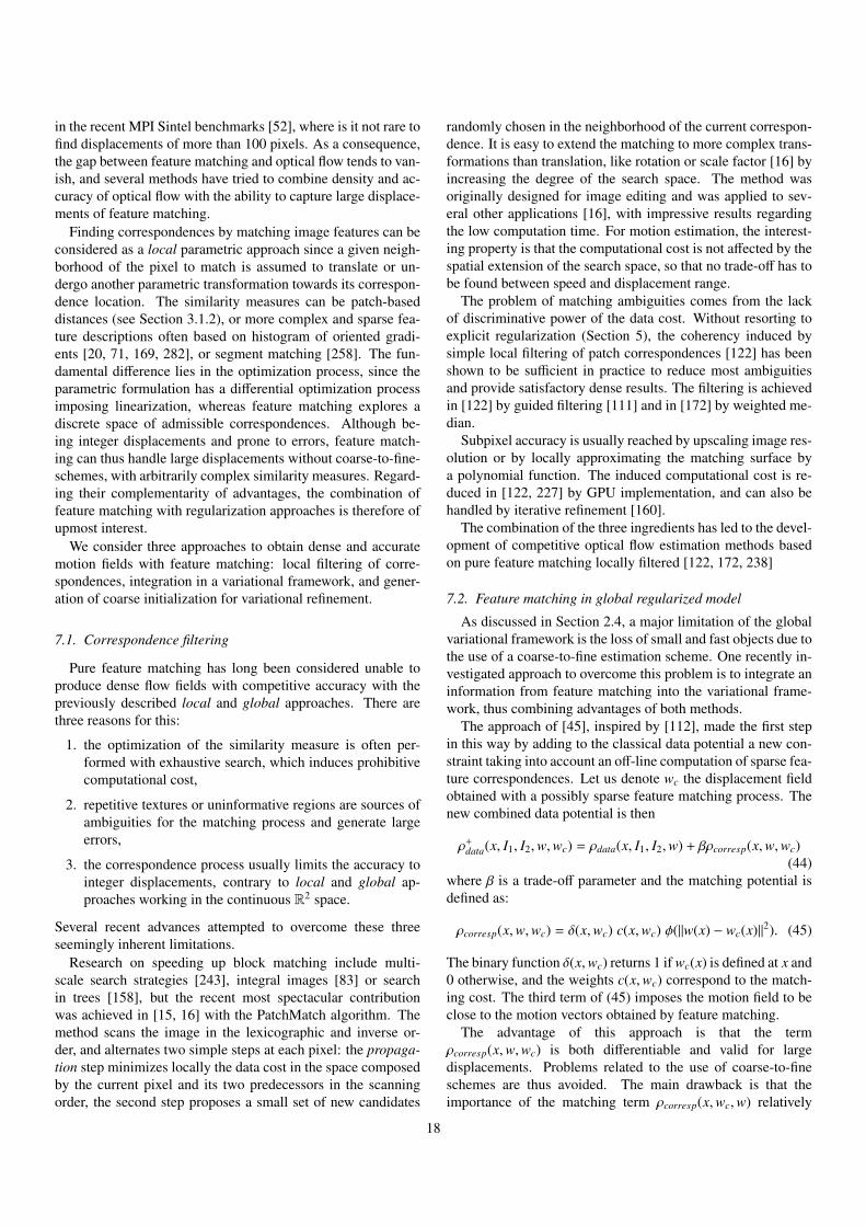
in the recent MPI Sintel benchmarks [52], where is it not rare tofind displacements of more than 100 pixels. As a consequence,the gap between feature matching and optical flow tends to van-ish, and several methods have tried to combine density and ac-curacy of optical flow with the ability to capture large displace-ments of feature matching.

Finding correspondences by matching image features can beconsidered as a local parametric approach since a given neigh-borhood of the pixel to match is assumed to translate or un-dergo another parametric transformation towards its correspon-dence location. The similarity measures can be patch-baseddistances (see Section 3.1.2), or more complex and sparse fea-ture descriptions often based on histogram of oriented gradi-ents [20, 71, 169, 282], or segment matching [258]. The fun-damental difference lies in the optimization process, since theparametric formulation has a differential optimization processimposing linearization, whereas feature matching explores adiscrete space of admissible correspondences. Although be-ing integer displacements and prone to errors, feature match-ing can thus handle large displacements without coarse-to-fine-schemes, with arbitrarily complex similarity measures. Regard-ing their complementarity of advantages, the combination offeature matching with regularization approaches is therefore ofupmost interest.

We consider three approaches to obtain dense and accuratemotion fields with feature matching: local filtering of corre-spondences, integration in a variational framework, and gener-ation of coarse initialization for variational refinement.

7.1. Correspondence filtering

Pure feature matching has long been considered unable toproduce dense flow fields with competitive accuracy with thepreviously described local and global approaches. There arethree reasons for this:

1. the optimization of the similarity measure is often per-formed with exhaustive search, which induces prohibitivecomputational cost,

2. repetitive textures or uninformative regions are sources ofambiguities for the matching process and generate largeerrors,

3. the correspondence process usually limits the accuracy tointeger displacements, contrary to local and global ap-proaches working in the continuous R2 space.

Several recent advances attempted to overcome these threeseemingly inherent limitations.

Research on speeding up block matching include multi-scale search strategies [243], integral images [83] or searchin trees [158], but the recent most spectacular contributionwas achieved in [15, 16] with the PatchMatch algorithm. Themethod scans the image in the lexicographic and inverse or-der, and alternates two simple steps at each pixel: the propaga-tion step minimizes locally the data cost in the space composedby the current pixel and its two predecessors in the scanningorder, the second step proposes a small set of new candidates

randomly chosen in the neighborhood of the current correspon-dence. It is easy to extend the matching to more complex trans-formations than translation, like rotation or scale factor [16] byincreasing the degree of the search space. The method wasoriginally designed for image editing and was applied to sev-eral other applications [16], with impressive results regardingthe low computation time. For motion estimation, the interest-ing property is that the computational cost is not affected by thespatial extension of the search space, so that no trade-off has tobe found between speed and displacement range.

The problem of matching ambiguities comes from the lackof discriminative power of the data cost. Without resorting toexplicit regularization (Section 5), the coherency induced bysimple local filtering of patch correspondences [122] has beenshown to be sufficient in practice to reduce most ambiguitiesand provide satisfactory dense results. The filtering is achievedin [122] by guided filtering [111] and in [172] by weighted me-dian.

Subpixel accuracy is usually reached by upscaling image res-olution or by locally approximating the matching surface bya polynomial function. The induced computational cost is re-duced in [122, 227] by GPU implementation, and can also behandled by iterative refinement [160].

The combination of the three ingredients has led to the devel-opment of competitive optical flow estimation methods basedon pure feature matching locally filtered [122, 172, 238]

7.2. Feature matching in global regularized model

As discussed in Section 2.4, a major limitation of the globalvariational framework is the loss of small and fast objects due tothe use of a coarse-to-fine estimation scheme. One recently in-vestigated approach to overcome this problem is to integrate aninformation from feature matching into the variational frame-work, thus combining advantages of both methods.

The approach of [45], inspired by [112], made the first stepin this way by adding to the classical data potential a new con-straint taking into account an off-line computation of sparse fea-ture correspondences. Let us denote wc the displacement fieldobtained with a possibly sparse feature matching process. Thenew combined data potential is then

ρ+data(x, I1, I2,w,wc) = ρdata(x, I1, I2,w) + βρcorresp(x,w,wc)

(44)where β is a trade-off parameter and the matching potential isdefined as:

ρcorresp(x,w,wc) = δ(x,wc) c(x,wc) φ(‖w(x) − wc(x)‖2). (45)

The binary function δ(x,wc) returns 1 if wc(x) is defined at x and0 otherwise, and the weights c(x,wc) correspond to the match-ing cost. The third term of (45) imposes the motion field to beclose to the motion vectors obtained by feature matching.

The advantage of this approach is that the termρcorresp(x,w,wc) is both differentiable and valid for largedisplacements. Problems related to the use of coarse-to-fineschemes are thus avoided. The main drawback is that theimportance of the matching term ρcorresp(x,wc,w) relatively

18

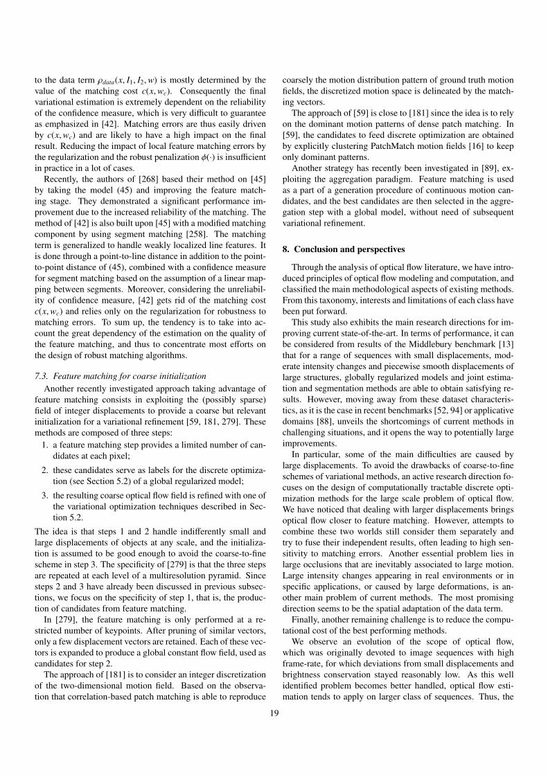
to the data term ρdata(x, I1, I2,w) is mostly determined by thevalue of the matching cost c(x,wc). Consequently the finalvariational estimation is extremely dependent on the reliabilityof the confidence measure, which is very difficult to guaranteeas emphasized in [42]. Matching errors are thus easily drivenby c(x,wc) and are likely to have a high impact on the finalresult. Reducing the impact of local feature matching errors bythe regularization and the robust penalization φ(·) is insufficientin practice in a lot of cases.

Recently, the authors of [268] based their method on [45]by taking the model (45) and improving the feature match-ing stage. They demonstrated a significant performance im-provement due to the increased reliability of the matching. Themethod of [42] is also built upon [45] with a modified matchingcomponent by using segment matching [258]. The matchingterm is generalized to handle weakly localized line features. Itis done through a point-to-line distance in addition to the point-to-point distance of (45), combined with a confidence measurefor segment matching based on the assumption of a linear map-ping between segments. Moreover, considering the unreliabil-ity of confidence measure, [42] gets rid of the matching costc(x,wc) and relies only on the regularization for robustness tomatching errors. To sum up, the tendency is to take into ac-count the great dependency of the estimation on the quality ofthe feature matching, and thus to concentrate most efforts onthe design of robust matching algorithms.

7.3. Feature matching for coarse initializationAnother recently investigated approach taking advantage of

feature matching consists in exploiting the (possibly sparse)field of integer displacements to provide a coarse but relevantinitialization for a variational refinement [59, 181, 279]. Thesemethods are composed of three steps:

1. a feature matching step provides a limited number of can-didates at each pixel;

2. these candidates serve as labels for the discrete optimiza-tion (see Section 5.2) of a global regularized model;

3. the resulting coarse optical flow field is refined with one ofthe variational optimization techniques described in Sec-tion 5.2.

The idea is that steps 1 and 2 handle indifferently small andlarge displacements of objects at any scale, and the initializa-tion is assumed to be good enough to avoid the coarse-to-finescheme in step 3. The specificity of [279] is that the three stepsare repeated at each level of a multiresolution pyramid. Sincesteps 2 and 3 have already been discussed in previous subsec-tions, we focus on the specificity of step 1, that is, the produc-tion of candidates from feature matching.

In [279], the feature matching is only performed at a re-stricted number of keypoints. After pruning of similar vectors,only a few displacement vectors are retained. Each of these vec-tors is expanded to produce a global constant flow field, used ascandidates for step 2.

The approach of [181] is to consider an integer discretizationof the two-dimensional motion field. Based on the observa-tion that correlation-based patch matching is able to reproduce

coarsely the motion distribution pattern of ground truth motionfields, the discretized motion space is delineated by the match-ing vectors.

The approach of [59] is close to [181] since the idea is to relyon the dominant motion patterns of dense patch matching. In[59], the candidates to feed discrete optimization are obtainedby explicitly clustering PatchMatch motion fields [16] to keeponly dominant patterns.

Another strategy has recently been investigated in [89], ex-ploiting the aggregation paradigm. Feature matching is usedas a part of a generation procedure of continuous motion can-didates, and the best candidates are then selected in the aggre-gation step with a global model, without need of subsequentvariational refinement.

8. Conclusion and perspectives

Through the analysis of optical flow literature, we have intro-duced principles of optical flow modeling and computation, andclassified the main methodological aspects of existing methods.From this taxonomy, interests and limitations of each class havebeen put forward.

This study also exhibits the main research directions for im-proving current state-of-the-art. In terms of performance, it canbe considered from results of the Middlebury benchmark [13]that for a range of sequences with small displacements, mod-erate intensity changes and piecewise smooth displacements oflarge structures, globally regularized models and joint estima-tion and segmentation methods are able to obtain satisfying re-sults. However, moving away from these dataset characteris-tics, as it is the case in recent benchmarks [52, 94] or applicativedomains [88], unveils the shortcomings of current methods inchallenging situations, and it opens the way to potentially largeimprovements.

In particular, some of the main difficulties are caused bylarge displacements. To avoid the drawbacks of coarse-to-fineschemes of variational methods, an active research direction fo-cuses on the design of computationally tractable discrete opti-mization methods for the large scale problem of optical flow.We have noticed that dealing with larger displacements bringsoptical flow closer to feature matching. However, attempts tocombine these two worlds still consider them separately andtry to fuse their independent results, often leading to high sen-sitivity to matching errors. Another essential problem lies inlarge occlusions that are inevitably associated to large motion.Large intensity changes appearing in real environments or inspecific applications, or caused by large deformations, is an-other main problem of current methods. The most promisingdirection seems to be the spatial adaptation of the data term.

Finally, another remaining challenge is to reduce the compu-tational cost of the best performing methods.

We observe an evolution of the scope of optical flow,which was originally devoted to image sequences with highframe-rate, for which deviations from small displacements andbrightness conservation stayed reasonably low. As this wellidentified problem becomes better handled, optical flow esti-mation tends to apply on larger class of sequences. Thus, the

19

gap between optical flow and other correspondence problemslike registration or feature matching progressively reduces andopens the way to unified correspondence methods.

Acknowledgements

This work was realized as part of the Quaero program,funded by OSEO, French State agency for innovation. Itwas also partly supported by the France-BioImaging projectgranted by the Investissement d’Avenir program, and by UMR144 CNRS of Institut Curie.

References

[1] S. Ali and M. Shah. Human action recognition in videos using kinematicfeatures and multiple instance learning. IEEE Trans. Pattern Analysisand Machine Intelligence, 32(2):288–303, 2010.

[2] L. Alvarez, J. Escların, M. Lefebure, and S. Javier. A PDE model forcomputing the optical flow. In Proc. XVI Congreso de ecuaciones difer-enciales y aplicaciones, pages 1349–1356, Las Palmas de Gran Canaria,Spain, September 1999.

[3] F. Amat, E. W. Myers, and P. J. Keller. Fast and robust optical flowfor time-lapse microscopy using super-voxels. Bioinformatics, 29(3):373–380, 2013.

[4] T. Amiaz and N. Kiryati. Piecewise-smooth dense optical flow via levelsets. International Journal of Computer Vision, 68(2):111–124, 2006.

[5] T. Amiaz, E. Lubetzky, and N. Kiryati. Coarse to over-fine optical flowestimation. Pattern Recognition, 40(9):2496–2503, 2007.

[6] P. Arias, G. Facciolo, V. Caselles, and G. Sapiro. A variational frame-work for exemplar-based image inpainting. International Journal ofComputer Vision, 93(3):319–347, 2011.

[7] G. Aubert, R. Deriche, and P. Kornprobst. Computing optical flow viavariational techniques. SIAM Journal on Applied Mathematics, 60(1):156–182, 1999.

[8] J.-F. Aujol, G. Gilboa, T. Chan, and S. Osher. Structure-texture imagedecomposition - modeling, algorithms, and parameter selection. Inter-national Journal of Computer Vision, 67(1):111–136, 2006.

[9] S. Ayer and H. Sawhney. Layered representation of motion video us-ing robust maximum-likelihood estimation of mixture models and MDLencoding. In IEEE Int. Conference on Computer Vision (ICCV), pages777–784, Boston, June 1995.

[10] A. Ayvaci, M. Raptis, and S. Soatto. Sparse occlusion detection withoptical flow. International Journal of Computer Vision, 97(3):322–338,2012.

[11] S. Baker and I. Matthews. Lucas-Kanade 20 years on: A unifying frame-work. International Journal of Computer Vision, 56(3):221–255, 2004.

[12] S. Baker, M. J. Black, J. Lewis, S. Roth, D. Scharstein, and R. Szeliski.A database and evaluation methodology for optical flow. In InternationalConference on Computer Vision (ICCV), pages 1–8, Rio de Janeiro,Brazil, October 2007.

[13] S. Baker, D. Scharstein, J. Lewis, S. Roth, M. Black, and R. Szeliski.A database and evaluation methodology for optical flow. InternationalJournal of Computer Vision, 92(1):1–31, 2011.

[14] C. Ballester, L. Garrido, V. Lazcano, and V. Caselles. A TV-L1 opticalflow method with occlusion detection. In Pattern Recognition, pages31–40, 2012.

[15] C. Barnes, E. Shechtman, A. Finkelstein, and D. B. Goldman. Patch-match: a randomized correspondence algorithm for structural imageediting. In ACM Trans. On Graphics, volume 28, page 24. ACM, 2009.

[16] C. Barnes, E. Shechtman, D. B. Goldman, and A. Finkelstein. The gen-eralized patchmatch correspondence algorithm. In European Conferenceon Computer Vision (ECCV), pages 29–43, 2010.

[17] J. Barron, D. Fleet, and S. Beauchemin. Evaluation of optical flow.International Journal of Computer Vision, 12(1):43–77, 1994.

[18] T. Basha, Y. Moses, and N. Kiryati. Multi-view scene flow estimation: Aview centered variational approach. International Journal of ComputerVision, 101(1):6–21, 2013.

[19] A. Basset, P. Bouthemy, and C. Kervrann. Recovery of motion patterns

and dominant paths in videos of crowded scenes. In International Con-ference on Image Processing (ICIP), Paris, October 2014.

[20] H. Bay, T. Tuytelaars, and L. Van Gool. Surf: Speeded up robust fea-tures. In European Conference Computer Vision (ECCV), pages 404–417, 2006.

[21] S. S. Beauchemin and J. L. Barron. The computation of optical flow.ACM Computing Surveys (CSUR), 27(3):433–466, 1995.

[22] F. Becker, B. Wieneke, S. Petra, A. Schroder, and C. Schnorr. Variationaladaptive correlation method for flow estimation. IEEE Trans. on ImageProcessing, 21(6):3053–3065, 2012.

[23] J. R. Bergen, P. Anandan, K. J. Hanna, and R. Hingorani. Hierarchicalmodel-based motion estimation. In European Conference on ComputerVision (ECCV), pages 237–252. Springer, 1992.

[24] M. Bertalmio, G. Sapiro, V. Caselles, and C. Ballester. Image inpainting.In Proceedings of the Annual Conference on Computer Graphics andInteractive Techniques, pages 417–424, 2000.

[25] J. Besag. On the statistical analysis of dirty pictures. Journal of the RoyalStatistical Society. Series B (Methodological), pages 259–302, 1986.

[26] J. Bigun, G. H. Granlund, and J. Wiklund. Multidimensional orientationestimation with applications to texture analysis and optical flow. IEEETrans. Pattern Analysis and Machine Intelligence, 13(8):775–790, 1991.

[27] M. Black and P. Anandan. The robust estimation of multiple motions:Parametric and piecewise-smooth flow fields. Computer Vision and Im-age Understanding, 63(1):75–104, 1996.

[28] M. Black and A. Jepson. Estimating optical flow in segmented im-ages using variable-order parametric models with local deformations.IEEE Trans. Pattern Analysis and Machine Intelligence, 18(10):972–986, 1996.

[29] M. J. Black. Recursive non-linear estimation of discontinuous flowfields. In European Conference on Computer Vision (ECCV), pages138–145, 1994.

[30] M. J. Black and P. Anandan. A framework for the robust estimation ofoptical flow. In International Conference on Computer Vision (ICCV),pages 231–236, 1993.

[31] M. J. Black and Y. Yacoob. Recognizing facial expressions in imagesequences using local parameterized models of image motion. Interna-tional Journal of Computer Vision, 25(1):23–48, 1997.

[32] M. J. Black, Y. Yacoob, A. D. Jepson, and D. J. Fleet. Learning pa-rameterized models of image motion. In Computer Vision and PatternRecognition (CVPR), pages 561–567, 1997.

[33] A. Blake and A. Zisserman. Visual reconstruction. MIT press Cam-bridge, 1987.

[34] M. Bleyer, C. Rhemann, and M. Gelautz. Segmentation-based motionwith occlusions using graph-cut optimization. In DAGM symposiumon Pattern Recognotion, pages 465–474, Berlin, Germany, September2006.

[35] E. Boros, P. Hammer, and X. Sun. Network flows and minimization ofquadratic pseudo-boolean functions. Technical report, Technical ReportRRR 17-1991, RUTCOR, 1991.

[36] J.-Y. Bouguet. Pyramidal implementation of the Lucas-Kanade featuretracker. Description of the algorithm. Technical report, Intel Micropro-cessor Research Labs, 1999.

[37] P. Bouthemy and E. Francois. Motion segmentation and qualitative dy-namic scene analysis from an image sequence. International Journal ofComputer Vision, 10(2):157–182, 1993.

[38] S. Boyd, N. Parikh, E. Chu, B. Peleato, and J. Eckstein. Distributedoptimization and statistical learning via the alternating direction methodof multipliers. Foundations and Trends R© in Machine Learning, 3(1):1–122, 2011.

[39] Y. Boykov, O. Veksler, and R. Zabih. Markov random fields with ef-ficient approximations. In Computer Vision and Pattern Recognition(CVPR), pages 648–655, 1998.

[40] Y. Boykov, O. Veksler, and R. Zabih. Fast approximate energy min-imization via graph cuts. IEEE Trans. Pattern Analysis and MachineIntelligence, 23(11):1222–1239, 2001.

[41] G. Bradski. Opencv. Dr. Dobb’s Journal of Software Tools, 2000.[42] J. Braux-Zin, R. Dupont, and A. Bartoli. A general dense image match-

ing framework combining direct and feature-based costs. In Interna-tional Conference on Computer Vision (ICCV), 2013.

[43] K. Bredies, K. Kunisch, and T. Pock. Total generalized variation. SIAMJournal on Imaging Sciences, 3(3):492–526, 2010.

20

[44] L. G. Brown. A survey of image registration techniques. ACM Comput-ing Surveys (CSUR), 24(4):325–376, 1992.

[45] T. Brox and J. Malik. Large displacement optical flow: descriptor match-ing in variational motion estimation. IEEE Trans. Pattern Analysis andMachine Intelligence, IEEE Trans. on, 33(3):500–513, 2011.

[46] T. Brox, A. Bruhn, N. Papenberg, and J. Weickert. High accuracy opti-cal flow estimation based on a theory for warping. In European Confer-ence on Computer Vision (ECCV), pages 25–36, Prague, Czech Repub-lic, May 2004.

[47] T. Brox, A. Bruhn, and J. Weickert. Variational motion segmentationwith level sets. European Conference on Computer Vision (ECCV),pages 471–483, 2006.

[48] T. Brox, J. Weickert, B. Burgeth, and P. Mrazek. Nonlinear structuretensors. Image and Vision Computing, 24(1):41–55, 2006.

[49] A. Bruhn and W. Weickert. A confidence measure for variational opticflow methods. Geometric Properties for Incomplete Data, pages 283 –298, 2006.

[50] A. Bruhn, J. Weickert, and C. Schnorr. Lucas/Kanade meetshorn/schunck: Combining local and global optic flow methods. Interna-tional Journal of Computer Vision, 61(3):211–231, 2005.

[51] A. Bugeau, M. Bertalmıo, V. Caselles, and G. Sapiro. A comprehensiveframework for image inpainting. IEEE Trans. on Image Processing, 19(10):2634–2645, 2010.

[52] D. J. Butler, J. Wulff, G. B. Stanley, and M. J. Black. A naturalistic opensource movie for optical flow evaluation. In European Conference onComputer Vision (ECCV), pages 611–625. Springer-Verlag, 2012.

[53] X. Cai, J. H. Fitschen, M. Nikolova, G. Steidl, and M. Storath. Dispar-ity and optical flow partitioning using extended Potts priors. Submittedto Information and Inference: A Journal of the IMA, 2014. PreprintarXiv:1405.1594.

[54] A. Chambolle. An algorithm for total variation minimization and appli-cations. Journal of Mathematical Imaging and Vision, 20(1-2):89–97,2004.

[55] A. Chambolle and T. Pock. A first-order primal-dual algorithm for con-vex problems with applications to imaging. Journal of MathematicalImaging and Vision, 40(1):120–145, 2011.

[56] T. F. Chan, S. H. Kang, and J. Shen. Euler’s elastica and curvature-based inpainting. SIAM Journal on Applied Mathematics, pages 564–592, 2002.

[57] H. Chao, Y. Gu, and M. Napolitano. A survey of optical flow techniquesfor robotics navigation applications. Journal of Intelligent & RoboticSystems, 73(1-4):361–372, 2014.

[58] P. Charbonnier, L. Blanc-Feraud, G. Aubert, and M. Barlaud. Determin-istic edge-preserving regularization in computed imaging. IEEE Trans.on Image Processing, 6(2):298–311, 1997.

[59] Z. Chen, H. Jin, Z. Lin, S. Cohen, and Y. Wu. Large displacement op-tical flow from nearest neighbor fields. In Computer Vision and PatternRecognition (CVPR), pages 2443–2450, 2013.

[60] T. M. Chin, W. C. Karl, and A. S. Willsky. Probabilistic and sequentialcomputation of optical flow using temporal coherence. IEEE Trans. onImage Processing, 3(6):773–788, 1994.

[61] P. Chou and C. Brown. The theory and practice of Bayesian image la-beling. International Journal of Computer Vision, 4(3):185–210, June1990.

[62] P. G. Ciarlet. The finite element method for elliptic problems. Elsevier,1978.

[63] I. Cohen. Nonlinear variational method for optical flow computation.In Proceedings of the 8th Scandinavian Conference on Image Analysis,pages 523–530, 1993.

[64] T. Cooke. Two applications of graph-cuts to image processing. In DigitalImage Computing: Techniques and Applications (DICTA), pages 498–504, 2008.

[65] T. Corpetti, E. Memin, and P. Perez. Dense estimation of fluid flows.IEEE Trans. Pattern Analysis and Machine Intelligence, 24(3):365–380,2002.

[66] D. Cremers and S. Soatto. Motion competition: A variational approachto piecewise parametric motion segmentation. International Journal ofComputer Vision, 62(3):249–265, 2005.

[67] A. Cretual and F. Chaumette. Visual servoing based on image motion.The International Journal of Robotics Research, 20(11):857–877, 2001.

[68] A. Criminisi, P. Perez, and K. Toyama. Region filling and object removal

by exemplar-based image inpainting. IEEE Trans. on Image Processing,13(9):1200–1212, 2004.

[69] T. Crivelli, B. Cernuschi-Frias, P. Bouthemy, and J.-F. Yao. Motiontextures: Modeling, classification, and segmentation using mixed-stateMarkov random fields. SIAM Journal on Imaging Sciences, 6(4):2484–2520, 2013.

[70] R. Cutler and M. Turk. View-based interpretation of real-time opticalflow for gesture recognition. In International Conference on AutomaticFace and Gesture Recognition, pages 416–416, 1998.

[71] N. Dalal and B. Triggs. Histograms of oriented gradients for human de-tection. In Computer Vision and Pattern Recognition (CVPR), volume 1,pages 886–893, 2005.

[72] J. Delon and B. Rouge. Small baseline stereovision. Journal of Mathe-matical Imaging and Vision, 28(3):209–223, 2007.

[73] J. Delpiano, J. Jara, J. Scheer, O. A. Ramırez, J. Ruiz-del Solar, andS. Hartel. Performance of optical flow techniques for motion analysisof fluorescent point signals in confocal microscopy. Machine Vision andApplications, 23(4):675–689, 2012.

[74] O. Demetz, M. Stoll, S. Volz, J. Weickert, and A. Bruhn. Learn-ing brightness transfer functions for the joint recovery of illuminationchanges and optical flow. In European Conference on Computer Vision(ECCV), pages 455–471, Zurich, September 2014.

[75] P. Derian, P. Heas, C. Herzet, and E. Memin. Wavelet-based fluid motionestimation. In Scale Space and Variational Methods in Computer Vision(SSVM), pages 737–748, 2011.

[76] P. Derian, P. Heas, C. Herzet, E. Memin, et al. Wavelets and opticalflow motion estimation. Numerical Mathematics: Theory, Methods andApplications, 6(1):117–137, 2013.

[77] R. Deriche, P. Kornprobst, and G. Aubert. Optical-flow estimation whilepreserving its discontinuities: a variational approach. In Recent Devel-opments in Computer Vision, pages 69–80. LNCS 1035, Springer, 1996.

[78] M. Drulea and S. Nedevschi. Total variation regularization of local-global optical flow. In Intelligent Transportation Systems Conference(ITSC), pages 318–323, 2011.

[79] M. Drulea and S. Nedevschi. Motion estimation using the correlationtransform. IEEE Trans. on Image Processing, 22(8):3260–3270, 2013.

[80] R. Dupont, N. Paragios, R. Keriven, and P. Fuchs. Extraction of layersof similar motion through combinatorial techniques. In Energy Mini-mization Methods in Computer Vision and Pattern Recognition, pages220–234. Springer, 2005.

[81] W. Enkelmann. Investigations of multigrid algorithms for the estimationof optical flow fields in image sequences. Computer Vision, Graphics,and Image Processing, 43(2):150–177, 1988.

[82] W. Enkelmann. Obstacle detection by evaluation of optical flow fieldsfrom image sequences. Image and Vision Computing, 9(3):160–168,1991.

[83] G. Facciolo, N. Limare, and E. Meinhardt. Integral images for blockmatching. Image Processing On Line, 2013.

[84] S. Fazekas and D. Chetverikov. Normal versus complete flow in dy-namic texture recognition: a comparative study. In Workshop on TextureAnalysis and Synthesis at International Conference on Computer Vision(ICCV), pages 37–42, Beijin, China, 2005.

[85] S. Fazekas, T. Amiaz, D. Chetverikov, and N. Kiryati. Dynamic texturedetection based on motion analysis. International Journal of ComputerVision, 82(1):48–63, 2009.

[86] A. Fix, A. Gruber, E. Boros, and R. Zabih. A graph cut algorithmfor higher-order Markov random fields. In International Conference onComputer Vision (ICCV), pages 1020–1027, 2011.

[87] D. J. Fleet, M. J. Black, Y. Yacoob, and A. D. Jepson. Design and useof linear models for image motion analysis. International Journal ofComputer Vision, 36(3):171–193, 2000.

[88] D. Fortun, P. Bouthemy, P. Paul-Gilloteaux, and C. Kervrann. Aggrega-tion of patch-based estimations for illumination-invariant optical flow inlive cell imaging. In International Symposium on Biomedical Imaging(ISBI), pages 660–663. IEEE, 2013.

[89] D. Fortun, P. Bouthemy, and C. Kervrann. Aggregation of local paramet-ric candidates with exemplar-based occlusion handling for optical flow.Preprint arXiv:1407.5759, June 2014.

[90] D. Fortun, C. Chen, P. Paul-Gilloteaux, F. Waharte, J. Salamero, andC. Kervrann. Correlation and variational approaches for motion anddiffusion estimation in fluorescence imaging. In European Signal Pro-

21

cessing Conference (EUSIPCO), pages 660–663, September 2013.[91] D. R. Fulkerson. Flows in networks. Princeton University Press, 1962.[92] R. Gal, N. Kiryati, and N. Sochen. Progress in the restoration of im-

age sequences degraded by atmospheric turbulence. Pattern RecognitionLetters, 14:8–14, October 2014.

[93] R. Garg, A. Roussos, and L. Agapito. Robust trajectory-space TV-L1optical flow for non-rigid sequences. In Energy Minimization Methodsin Computer Vision and Pattern Recognition (EMMCVPR), pages 300–314. Springer, 2011.

[94] A. Geiger, P. Lenz, and R. Urtasun. Are we ready for autonomous driv-ing? the KITTI vision benchmark suite. In Computer Vision and PatternRecognition (CVPR), pages 3354–3361, 2012.

[95] M. Gelgon, P. Bouthemy, and T. Dubois. A region tracking method withfailure detection for an interactive video indexing environment. In VisualInformation and Information Systems, pages 261–269. Springer, 1999.

[96] D. Geman and G. Reynolds. Constrained restoration and the recovery ofdiscontinuities. IEEE Trans. Pattern Analysis and Machine Intelligence,14(3):367–383, 1992.

[97] S. Geman and D. Geman. Stochastic relaxation, Gibbs distributions, andthe Bayesian restoration of images. IEEE Trans. Pattern Analysis andMachine Intelligence, (6):721–741, 1984.

[98] A. Giachetti, M. Campani, and V. Torre. The use of optical flow for roadnavigation. IEEE Trans. Robotics and Automation, 14(1):34–48, 1998.

[99] B. Glocker, N. Komodakis, N. Paragios, G. Tziritas, and N. Navab. In-ter and intra-modal deformable registration: Continuous deformationsmeet efficient optimal linear programming. In Information Processingin Medical Imaging (IPMI), pages 408–420. Springer, 2007.

[100] B. Glocker, N. Paragios, N. Komodakis, G. Tziritas, and N. Navab. Opti-cal flow estimation with uncertainties through dynamic MRFs. In Com-puter Vision and Pattern Recognition (CVPR), pages 1–8, Anchorage,Alaska, June 2008.

[101] B. Glocker, T. Heibel, N. Navab, P. Kohli, and C. Rother. Triangleflow:Optical flow with triangulation-based higher-order likelihoods. Euro-pean Conference on Computer Vision (ECCV), pages 272–285, 2010.

[102] A. V. Goldberg and R. E. Tarjan. A new approach to the maximum-flowproblem. Journal of the ACM (JACM), 35(4):921–940, 1988.

[103] P. Golland and A. M. Bruckstein. Motion from color. Computer Visionand Image Understanding, 68(3):346–362, 1997.

[104] S. Grauer-Gray and C. Kambhamettu. Hierarchical belief propagationto reduce search space using cuda for stereo and motion estimation.In Workshop on Applications of Computer Vision (WACV), pages 1–8,2009.

[105] S. Grewenig, J. Weickert, and A. Bruhn. From box filtering to fast ex-plicit diffusion. In DAGM symposium on Pattern Recognition, pages533–542, 2010.

[106] M. D. Grossberg and S. K. Nayar. Modeling the space of camera re-sponse functions. IEEE Trans. Pattern Analysis and Machine Intelli-gence, 26(10):1272–1282, 2004.

[107] P. Gwosdek, H. Zimmer, S. Grewenig, A. Bruhn, and J. Weickert. Ahighly efficient GPU implementation for variational optic flow based onthe Euler-Lagrange framework. In Trends and Topics in Computer Vi-sion, pages 372–383, 2012.

[108] D. Hafner, O. Demetz, and J. Weickert. Why is the census transformgood for robust optic flow computation? In Scale Space and VariationalMethods in Computer Vision (SSVM), pages 210–221, 2013.

[109] N. Hata, A. Nabavi, W. M. Wells III, S. K. Warfield, R. Kikinis, P. M.Black, and F. A. Jolesz. Three-dimensional optical flow method for mea-surement of volumetric brain deformation from intraoperative mr im-ages. Journal of Computer Assisted Tomography, 24(4):531–538, 2000.

[110] H. W. Haussecker and D. J. Fleet. Computing optical flow with phys-ical models of brightness variation. IEEE Trans. Pattern Analysis andMachine Intelligence, 23(6):661–673, 2001.

[111] K. He, J. Sun, and X. Tang. Guided image filtering. In European Con-ference on Computer Vision (ECCV), pages 1–14, 2010.

[112] P. Heas, E. Memin, N. Papadakis, and A. Szantai. Layered estimationof atmospheric mesoscale dynamics from satellite imagery. Trans. onGeoscience and Remote Sensing, 45(12):4087–4104, 2007.

[113] P. Heas, C. Herzet, and E. Memin. Bayesian inference of models and hy-perparameters for robust optical-flow estimation. IEEE Trans. on ImageProcessing, 21(4):1437–1451, 2012.

[114] P. Heise, S. Klose, B. Jensen, and A. Knoll. PM-Huber: Patchmatch with

Huber regularization for stereo matching. In International Conferenceon Computer Vision (ICCV), 2013.

[115] D. Heitz, E. Memin, and C. Schnorr. Variational fluid flow measure-ments from image sequences: synopsis and perspectives. Experimentsin fluids, 48(3):369–393, 2010.

[116] F. Heitz and P. Bouthemy. Multimodal estimation of discontinuous opti-cal flow using Markov random fields. IEEE Trans. Pattern Analysis andMachine Intelligence, 15(12):1217–1232, 1993.

[117] F. Heitz, P. Perez, and P. Bouthemy. Multiscale minimization of globalenergy functions in some visual recovery problems. CVGIP : ImageUnderstanding, 59(1):125–134, Jan. 1994.

[118] S. Hermann and R. Klette. Hierarchical scan-line dynamic programmingfor optical flow using semi-global matching. In Workshops of AsianConference Computer Vision, pages 556–567. Springer, 2013.

[119] P. W. Holland and R. E. Welsch. Robust regression using iterativelyreweighted least-squares. Communications in Statistics-Theory andMethods, 6(9):813–827, 1977.

[120] B. Horn and B. Schunck. Determining optical flow. Artificial intelli-gence, 17(1-3):185–203, 1981.

[121] M. Hornacek, F. Besse, J. Kautz, A. Fitzgibbon, and C. Rother. Highlyoverparameterized optical flow using PatchMatch belief propagation.In European Conference on Computer Vision (ECCV), volume LNCS8689, Part III, pages 220–234, Zurich, September 2014.

[122] A. Hosni, C. Rhemann, M. Bleyer, C. Rother, and M. Gelautz. Fast cost-volume filtering for visual correspondence and beyond. IEEE Trans.Pattern Analysis and Machine Intelligence, 35(2):504–511, 2013.

[123] W. Hu, N. Xie, L. Li, X. Zeng, and S. Maybank. A survey on visualcontent-based video indexing and retrieval. IEEE Trans. on Systems,Man, and Cybernetics, 41(6):797–819, 2011.

[124] T.-C. Huang, C.-K. Chang, C.-H. Liao, and Y.-J. Ho. Quantification ofblood flow in internal cerebral artery by optical flow method on digi-tal subtraction angiography in comparison with time-of-flight magneticresonance angiography. PloS one, 8(1):54678, 2013.

[125] P. J. Huber. Robust statistics. Springer, 1981.[126] A. Humayun, O. Mac Aodha, and G. J. Brostow. Learning to find oc-

clusion regions. In Computer Vision and Pattern Recognition (CVPR),pages 2161–2168, 2011.

[127] S. Ince and J. Konrad. Occlusion-aware optical flow estimation. IEEETrans. on Image Processing, 17(8):1443–1451, 2008.

[128] H. Ishikawa. Higher-order clique reduction in binary graph cut. In Com-puter Vision and Pattern Recognition (CVPR), pages 2993–3000, 2009.

[129] N. Jacobson, Y. Freund, and T. Nguyen. An online learning approach toocclusion boundary detection. IEEE Trans. on Image Processing, 21(1):252–261, Jan. 2012.

[130] M. Jain, H. Jegou, and P. Bouthemy. Better exploiting motion for bet-ter action recognition. In Computer Vision and Pattern Recognition(CVPR), pages 2555–2562, Portland, Oregon, June 2013.

[131] M. Jakubowski and G. Pastuszak. Block-based motion estimation algo-rithmsa survey. Opto-Electronics Review, 21(1):86–102, 2013.

[132] P.-M. Jodoin and M. Mignotte. Optical-flow based on an edge-avoidanceprocedure. Computer Vision and Image Understanding, 113(4):511–531, 2009.

[133] S. Ju, M. Black, and A. Jepson. Skin and bones: Multi-layer, locallyaffine, optical flow and regularization with transparency. In ComputerVision and Pattern Recognition (CVPR), pages 307–314, 1996.

[134] E. M. Kalmoun and L. Garrido. Trust region versus line search for com-puting the optical flow. Multiscale Modeling & Simulation, 11(3):890–906, 2013.

[135] E. M. Kalmoun, L. Garrido, and V. Caselles. Line search multileveloptimization as computational methods for dense optical flow. SIAMJournal on Imaging Sciences, 4(2):695–722, 2011.

[136] J. H. Kappes, B. Andres, F. A. Hamprecht, C. Schnorr, S. Nowozin,D. Batra, S. Kim, B. X. Kausler, J. Lellmann, N. Komodakis, et al. Acomparative study of modern inference techniques for discrete energyminimization problems. In Computer Vision and Pattern Recognition(CVPR), 2013.

[137] C. Kervrann and F. Heitz. Statistical deformable model-based segmenta-tion of image motion. Trans. on Image Processing, 8(4):583–588, 1999.

[138] C. Kervrann, J. Boulanger, T. Pecot, P. Perez, and J. Salamero. Mul-tiscale neighborhood-wise decision fusion for redundancy detection inimage pairs. SIAM Journal Multiscale Modeling & Simulation, 9(4):

22

1829–1865, 2011.[139] I.-H. Kim, Y.-C. M. Chen, D. L. Spector, R. Eils, and K. Rohr. Nonrigid

registration of 2-d and 3-d dynamic cell nuclei images for improved clas-sification of subcellular particle motion. IEEE Trans. on Image Process-ing, 20(4):1011–1022, 2011.

[140] T. H. Kim, H. S. Lee, and K. M. Lee. Optical flow via locally adap-tive fusion of complementary data costs. International Conference onComputer Vision (ICCV), 2013.

[141] Y. Kim, A. Martınez, and A. Kak. A local approach for robust opticalflow estimation under varying illumination. In British Machine VisionConference (BMVC), pages 91–1, 2004.

[142] Y.-H. Kim, A. M. Martınez, and A. C. Kak. Robust motion estimationunder varying illumination. Image and Vision Computing, 23(4):365–375, 2005.

[143] N. Kiryati, T. R. Raviv, Y. Ivanchenko, and S. Rochel. Real-time abnor-mal motion detection in surveillance video. In International Conferenceon Pattern Recognition (ICPR), pages 1–4, 2008.

[144] P. Kohli and P. H. Torr. Dynamic graph cuts for efficient inference inMarkov random fields. IEEE Trans. Pattern Analysis and Machine In-telligence, 29(12):2079–2088, 2007.

[145] P. Kohli, M. P. Kumar, and P. H. Torr. P3 & beyond: Move making algo-rithms for solving higher order functions. IEEE Trans. Pattern Analysisand Machine Intelligence, 31(9):1645–1656, 2009.

[146] D. L. Kolin and P. W. Wiseman. Advances in image correlation spec-troscopy: measuring number densities, aggregation states, and dynamicsof fluorescently labeled macromolecules in cells. Cell biochemistry andbiophysics, 49(3):141–164, 2007.

[147] V. Kolmogorov. Convergent tree-reweighted message passing for energyminimization. IEEE Trans. Pattern Analysis and Machine Intelligence,28(10):1568–1583, 2006.

[148] V. Kolmogorov and C. Rother. Minimizing nonsubmodular functionswith graph cuts-a review. IEEE Trans. Pattern Analysis and MachineIntelligence, 29(7):1274–1279, 2007.

[149] V. Kolmogorov and R. Zabih. Computing visual correspondences withocclusion using graph cuts. In IEEE Int. Conference on Computer Vision(ICCV), July 2001.

[150] N. Komodakis and N. Paragios. Beyond pairwise energies: Efficientoptimization for higher-order MRFs. In Computer Vision and PatternRecognition (CVPR), pages 2985–2992, 2009.

[151] N. Komodakis and G. Tziritas. Image completion using efficient beliefpropagation via priority scheduling and dynamic pruning. IEEE Trans.on Image Processing, 16(11):2649–2661, 2007.

[152] N. Komodakis, G. Tziritas, and N. Paragios. Performance vs computa-tional efficiency for optimizing single and dynamic MRFs: Setting thestate of the art with primal-dual strategies. Computer Vision and ImageUnderstanding, 112(1):14–29, 2008.

[153] J. Konrad and E. Dubois. Bayesian estimation of motion vector fields.IEEE Trans. Pattern Analysis and Machine Intelligence, 14(9):910–927,1992.

[154] P. Krahenbuhl and V. Koltun. Efficient nonlocal regularization for opticalflow. In European Conference on Computer Vision (ECCV), pages 356–369, 2012.

[155] K. Krajsek and R. Mester. On the equivalence of variational and statis-tical differential motion estimation. In Southwest Symposium on ImageAnalysis and Interpretation, pages 11–15, 1996.

[156] K. Krajsek and R. Mester. Bayesian model selection for optical flowestimation. Pattern Recognition, 4713:142–151, 2007.

[157] F. R. Kschischang, B. J. Frey, and H.-A. Loeliger. Factor graphs andthe sum-product algorithm. IEEE Trans. on Information Theory, 47(2):498–519, 2001.

[158] N. Kumar, L. Zhang, and S. Nayar. What is a good nearest neighbors al-gorithm for finding similar patches in images? In European Conferenceon Computer Vision (ECCV), pages 364–378, 2008.

[159] S.-H. Lai. Robust image matching under partial occlusion and spatiallyvarying illumination change. Computer Vision and Image Understand-ing, 78(1):84–98, 2000.

[160] K. Lee, D. Kwon, I. Yun, and S. Lee. Optical flow estimation with adap-tive convolution kernel prior on discrete framework. In Computer Visionand Pattern Recognition (CVPR), pages 2504–2511, San Fransisco, June2010.

[161] V. Lempitsky, C. Rother, S. Roth, and A. Blake. Fusion moves for

Markov random field optimization. IEEE Trans. Pattern Analysis andMachine Intelligence, 32(8):1392–1405, 2010.

[162] M. Leordeanu, A. Zanfir, and C. Sminchisescu. Locally affine sparse-to-dense matching for motion and occlusion estimation. In InternationalConference on Computer Vision (ICCV), 2013.

[163] J. Lewis. Fast normalized cross-correlation. Vision Interface, pages120–123, 1995.

[164] W. Li, D. Cosker, M. Brown, and R. Tang. Optical flow estimation usingLaplacian mesh energy. In Computer Vision and Pattern Recognition(CVPR), pages 2435–2442, June 2013.

[165] C. Liu. Beyond pixels: exploring new representations and applicationsfor motion analysis. PhD thesis, Massachusetts Institute of Technology,2009.

[166] C. Liu, J. Yuen, and A. Torralba. Sift flow: Dense correspondence acrossscenes and its applications. IEEE Trans. Pattern Analysis and MachineIntelligence, 33(5):978–994, 2011.

[167] K. Liu, S. S. Lienkamp, A. Shindo, J. B. Wallingford, G. Walz, andO. Ronneberger. Optical flow guided cell segmentation and tracking indeveloping tissue. In International Symposium on Biomedical Imaging(ISBI), pages 298–301, 2014.

[168] T. Liu and L. Shen. Fluid flow and optical flow. Journal of Fluid Me-chanics, 614:253–291, 2008.

[169] D. G. Lowe. Distinctive image features from scale-invariant keypoints.International Journal of Computer Vision, 60(2):91–110, 2004.

[170] B. Lucas and T. Kanade. An iterative image registration technique withan application to stereo vision. International Joint Conference on Artifi-cial Intelligence, pages 674–679, 1981.

[171] J. Luo and E. E. Konofagou. A fast normalized cross-correlation calcu-lation method for motion estimation. IEE Trans. on Ultrasonics, Ferro-electrics and Frequency Control, 57(6):1347–1357, 2010.

[172] Z. Ma, K. He, Y. Wei, J. Sun, and E. Wu. Constant time weighted medianfiltering for stereo matching and beyond. International Conference onComputer Vision (ICCV), 2013.

[173] M. Maurizot, P. Bouthemy, B. Delyon, A. Juditski, and J. M. Odobez.Determination of singular points in 2d deformable flow fields. In InInternational Conference on Image Processing (ICIP), volume 3, pages488–491, 1995.

[174] E. Memin and P. Perez. Dense estimation and object-based segmenta-tion of the optical flow with robust techniques. IEEE Trans. on ImageProcessing, 7(5):703–719, 1998.

[175] E. Memin and P. Perez. Hierarchical estimation and segmentation ofdense motion fields. International Journal of Computer Vision, 46(2):129–155, 2002.

[176] Y. Mileva, A. Bruhn, and J. Weickert. Illumination-robust variationaloptical flow with photometric invariants. Pattern Recognition, pages152–162, 2007.

[177] A. Mitiche and J. K. Aggarwal. Computer Vision Analysis of ImageMotion by Variational Methods. Springer, 2014.

[178] A. Mitiche and P. Bouthemy. Computation and analysis of image mo-tion: A synopsis of current problems and methods. International Journalof Computer Vision, 19(1):29–55, 1996.

[179] M. A. Mohamed and B. Mertsching. TV-L1 optical flow estimation withimage details recovering based on modified census transform. In Ad-vances in Visual Computing, pages 482–491, 2012.

[180] J. Molnar, D. Chetverikov, and S. Fazekas. Illumination-robust varia-tional optical flow using cross-correlation. Computer Vision and ImageUnderstanding, 114(10):1104–1114, 2010.

[181] M. Mozerov. Constrained optical flow estimation as a matching prob-lem. IEEE Trans. on Image Processing, 22(5):2044–2055, 2013.

[182] T. Muller, C. Rabe, J. Rannacher, U. Franke, and R. Mester.Illumination-robust dense optical flow using census signatures. In Pat-tern Recognition, pages 236–245. LNCS 6835, Springer, 2011.

[183] T. Muller, J. Rannacher, C. Rabe, and U. Franke. Feature-and depth-supported modified total variation optical flow for 3d motion field es-timation in real scenes. In Computer Vision and Pattern Recognition(CVPR), pages 1193–1200, 2011.

[184] D. Mumford and J. Shah. Optimal approximations by piecewise smoothfunctions and associated variational problems. Communications on Pureand Applied Mathematics, 42(5):577–685, 1989.

[185] D. W. Murray and B. F. Buxton. Scene segmentation from visual motionusing global optimization. IEEE Trans. Pattern Analysis and Machine

23

Intelligence, 9(2):220–228, 1987.[186] H. Nagel and W. Enkelmann. An investigation of smoothness constraints

for the estimation of displacement vector fields from image sequences.IEEE Trans. Pattern Analysis and Machine Intelligence, 8(5):565–593,1986.

[187] H.-H. Nagel. Extending the oriented smoothness constraint into the tem-poral domain and the estimation of derivatives of optical flow. In Euro-pean Conference on Computer Vision (ECCV), pages 139–148, 1990.

[188] S. Negahdaripour. Revised definition of optical flow: Integration of ra-diometric and geometric cues for dynamic scene analysis. IEEE Trans.Pattern Analysis and Machine Intelligence, 20(9):961–979, 1998.

[189] L. Ng and V. Solo. Errors-in-variables modelling in optical flow prob-lems. In International Conference on Acoustics, Speech and Signal Pro-cessing (ICASSP), volume 5, pages 2773–2776, 1998.

[190] C. Nieuwenhuis, D. Kondermann, and C. S. Garbe. Complex motionmodels for simple optical flow estimation. In Pattern Recognition, pages141–150. LNCS 6376, Springer, 2010.

[191] T. Nir, A. M. Bruckstein, and R. Kimmel. Over-parameterized varia-tional optical flow. International Journal of Computer Vision, 76(2):205–216, 2008.

[192] P. Ochs, Y. Chen, T. Brox, and T. Pock. iPiano: Inertial proximal algo-rithm for non-convex optimization. SIAM Journal on Imaging Science,7(2):1388–1419, 2013.

[193] J. M. Odobez and P. Bouthemy. Robust multiresolution estimation ofparametric motion models. Journal of Visual Vommunication and ImageRepresentation, 6(4):348–365, 1995.

[194] J. M. Odobez and P. Bouthemy. Separation of moving regions frombackground in an image sequence acquired with a mobile camera. InH.-H. Li, S. Sun, and H. Derin, editors, Video Data Compression forMultimedia Computing, volume 378 of Series in Engineering and Com-puter Science, chapter 8, pages 283–311. Springer, 1997.

[195] J. M. Odobez and P. Bouthemy. Direct incremental model-based imagemotion segmentation for video analysis. Signal Processing, 66(2):143–155, 1998.

[196] G. Panin. Mutual information for multi-modal, discontinuity-preservingimage registration. In Advances in Visual Computing, pages 70–81,2012.

[197] N. Papadakis, R. Yildizoglu, J.-F. Aujol, and V. Caselles. High-dimension multilabel problems: Convex or nonconvex relaxation? SIAMJournal on Imaging Sciences, 6(4):2603–2639, 2013.

[198] N. Papenberg, A. Bruhn, T. Brox, S. Didas, and J. Weickert. Highlyaccurate optic flow computation with theoretically justified warping. In-ternational Journal of Computer Vision, 67(2):141–158, 2006.

[199] N. Paragios and R. Deriche. Geodesic active regions and level set meth-ods for motion estimation and tracking. Computer Vision and ImageUnderstanding, 97(3):259–282, 2005.

[200] J. Pearl. Probabilistic reasoning in intelligent systems: networks of plau-sible inference. Morgan Kaufmann, 1988.

[201] M. Pingault, E. Bruno, and D. Pellerin. A robust multisacle B-splinefunction decomposition for estimating motion transparency. IEEETrans. on Image Processing, 12(11):1416–1426, Nov. 2003.

[202] G. Piriou, P. Bouthemy, and J.-F. Yao. Recognition of dynamic videocontents with global probabilistic models of visual motion. IEEE Trans.on Image Processing, 15(11):3417–3430, Nov. 2006.

[203] L. Pizarro, J. Delpiano, P. Aljabar, J. Ruiz-del Solar, and D. Rueck-ert. Towards dense motion estimation in light and electron microscopy.In International Symposium on Biological Imaging (ISBI), pages 1939–1942, 2011.

[204] T. Pock, M. Pock, and H. Bischof. Algorithmic differentiation: Appli-cation to variational problems in computer vision. IEEE Trans. PatternAnalysis and Machine Intelligence, 29(7):1180–1193, 2007.

[205] R. Ranftl, S. Gehrig, T. Pock, and H. Bischof. Pushing the limits ofstereo using variational stereo estimation. In Intelligent Vehicles Sympo-sium (IV), pages 401–407, 2012.

[206] H. A. Rashwan, M. A. Garcıa, and D. Puig. Variational optical flow esti-mation based on stick tensor voting. IEEE Trans. on Image Processing,22(7):2589–2599, 2013.

[207] T. Riklin-Raviv, N. Sochen, and N. Kiryati. Shape-based mutual seg-mentation. International Journal of Computer Vision, 79(3):231–245,2008.

[208] S. Roth and M. Black. On the spatial statistics of optical flow. Interna-

tional Journal of Computer Vision, 74(1):33–50, 2007.[209] C. Rother, V. Kolmogorov, V. Lempitsky, and M. Szummer. Optimizing

binary MRFs via extended roof duality. In Computer Vision and PatternRecognition (CVPR), pages 1–8, 2007.

[210] L. I. Rudin, S. Osher, and E. Fatemi. Nonlinear total variation basednoise removal algorithms. Physica D: Nonlinear Phenomena, 60(1):259–268, 1992.

[211] D. Rueckert, L. I. Sonoda, C. Hayes, D. L. Hill, M. O. Leach, and D. J.Hawkes. Nonrigid registration using free-form deformations: applica-tion to breast MR images. IEEE Trans. Pattern Analysis and MachineIntelligence, 18(8):712–721, 1999.

[212] J. A. Schnabel, D. Rueckert, M. Quist, J. M. Blackall, A. D. Castellano-Smith, T. Hartkens, G. P. Penney, W. A. Hall, H. Liu, C. L. Truwit,et al. A generic framework for non-rigid registration based on non-uniform multi-level free-form deformations. In Medical Image Com-puting and Computer-Assisted Intervention (MICCAI), pages 573–581.Springer, 2001.

[213] C. Schnorr and W. Peckar. Motion-based identification of deformabletemplates. In International Conference Computer Analysis of Imagesand Patterns (CAIP), pages 122–129, Prague, 1995.

[214] T. Schoenemann and D. Cremers. Near real-time motion segmentationusing graph cuts. In DAGM Symposium on Pattern Recognition, pages455–464, 2006.

[215] T. Senst, V. Eiselen, and T. Sikora. Robust local optical flow for featuretracking. IEEE Trans. on Circuits and Systems for Video Technology, 22(9):1377–1387, 2012.

[216] A. Shekhovtsov, I. Kovtun, and V. Hlavavc. Efficient MRF deforma-tion model for non-rigid image matching. Computer Vision and ImageUnderstanding, 112(1):91–99, 2008.

[217] X. Shen and Y. Wu. Sparsity model for robust optical flow estimationat motion discontinuities. In Computer Vision and Pattern Recognition(CVPR), pages 2456–2463, 2010.

[218] J. Shi and C. Tomasi. Good features to track. In Computer Vision andPattern Recognition (CVPR), pages 593–600, 1994.

[219] W. Shi, X. Zhuang, L. Pizarro, W. Bai, H. Wang, K.-P. Tung, P. Edwards,and D. Rueckert. Registration using sparse free-form deformations. InMedical Image Computing and Computer-Assisted Intervention (MIC-CAI), pages 659–666, 2012.

[220] D. Shulman and J.-Y. Herve. Regularization of discontinuous flow fields.In Workshop on Visual Motion, pages 81–86, 1989.

[221] E. P. Simoncelli, E. H. Adelson, and D. J. Heeger. Probability distri-butions of optical flow. In Computer Vision and Pattern Recognition(CVPR), pages 310–315, 1991.

[222] S. N. Sinha, J.-M. Frahm, M. Pollefeys, and Y. Genc. Feature trackingand matching in video using programmable graphics hardware. MachineVision and Applications, 22(1):207–217, 2011.

[223] P. Smith, T. Drummond, and R. Cipolla. Layered motion segmentationand depth ordering by tracking edges. IEEE Trans. Pattern Analysis andMachine Intelligence, 26(4):479–494, April 2004.

[224] A. Sotiras, C. Davatzikos, and N. Paragios. Deformable medical imageregistration: A survey. IEEE Trans. on Medical Imaging, 32(7):1153–1190, 2013.

[225] A. N. Stein and M. Hebert. Occlusion boundaries from motion: Low-level detection and mid-level reasoning. International Journal of Com-puter Vision, 82(3):325–357, 2009.

[226] F. Stein. Efficient computation of optical flow using the census trans-form. In Pattern Recognition, pages 79–86. LNCS 3175, Springer, 2004.

[227] F. Steinbrucker, T. Pock, and D. Cremers. Advanced data terms forvariational optic flow estimation. In Vision, Modeling, and VisualizationWorkshop, 2009.

[228] C. Stiller and J. Konrad. Estimating motion in image sequences. IEEESignal Processing Magazine, 16(4):70–91, July 1999.

[229] C. Strecha, R. Fransens, and L. Van Gool. A probabilistic approach tolarge displacement optical flow and occlusion detection. In Statisticalmethods in video processing, pages 71–82. Springer, 2004.

[230] C.-W. Su, H.-Y. Liao, H.-R. Tyan, C.-W. Lin, D.-Y. Chen, and K.-C.Fan. Motion flow-based video retrieval. IEEE Trans. on Multimedia, 9(6):1193–1201, 2007.

[231] D. Sun, S. Roth, J. Lewis, and M. Black. Learning optical flow. InEuropean Conference on Computer Vision (ECCV), pages 83–97, 2008.

[232] D. Sun, S. Roth, and M. Black. Secrets of optical flow estimation and

24

their principles. In Computer Vision and Pattern Recognition (CVPR),pages 2432–2439, San Fransisco, June 2010.

[233] D. Sun, E. Sudderth, and M. Black. Layered image motion with explicitocclusions, temporal consistency, and depth ordering. In Advances inNeural Information Processing Systems (NIPS), pages 2226–2234, Van-couver, December 2010.

[234] D. Sun, E. B. Sudderth, and M. J. Black. Layered segmentation and op-tical flow estimation over time. In Computer Vision and Pattern Recog-nition (CVPR), pages 1768–1775, 2012.

[235] Z. Sun, G. Bebis, and R. Miller. On-road vehicle detection: A review.IEEE Trans. Pattern Analysis and Machine Intelligence, 28(5):694–711,2006.

[236] R. Szeliski and H.-Y. Shum. Motion estimation with quadtree splines.IEEE Trans. Pattern Analysis and Machine Intelligence, 18(12):1199–1210, 1996.

[237] R. Szeliski, R. Zabih, D. Scharstein, O. Veksler, V. Kolmogorov,A. Agarwala, M. Tappen, and C. Rother. A comparative study of energyminimization methods for markov random fields with smoothness-basedpriors. IEEE Trans. Pattern Analysis and Machine Intelligence, 30(6):1068–1080, 2008.

[238] M. Tao, J. Bai, P. Kohli, and S. Paris. Simpleflow: A non-iterative, sub-linear optical flow algorithm. In Computer Graphics Forum, volume 31,pages 345–353, 2012.

[239] C.-H. Teng, S.-H. Lai, Y.-S. Chen, and W.-H. Hsu. Accurate optical flowcomputation under non-uniform brightness variations. Computer Visionand Image Understanding, 97(3):315–346, 2005.

[240] M. Tistarelli. Multiple constraints to compute optical flow. IEEE Trans.Pattern Analysis and Machine Intelligence, 18(12):1243–1250, 1996.

[241] Trobin, T. Pock, D. Cremers, and H. Bischof. An unbiased second-order prior for high-accuracy motion estimation. DAGM symposium onPattern Recognition, pages 396–405, 2008.

[242] W. Trobin, T. Pock, D. Cremers, and H. Bischof. Continuous energyminimization via repeated binary fusion. In European Conference onComputer Vision (ECCV), pages 677–690, Marseille, France, October2008.

[243] D. Tzovaras, M. G. Strintzis, and H. Sahinoglou. Evaluation of multires-olution block matching techniques for motion and disparity estimation.Signal Processing: Image Communication, 6(1):59–67, 1994.

[244] M. Unger, M. Werlberger, T. Pock, and H. Bischof. Joint motion estima-tion and segmentation of complex scenes with label costs and occlusionmodeling. In Computer Vision and Pattern Recognition (CVPR), pages1878–1885, 2012.

[245] S. Uras, F. Girosi, A. Verri, and V. Torre. A computational approach tomotion perception. Biological Cybernetics, 60(2):79–87, 1988.

[246] J. van de Weijer and T. Gevers. Robust optical flow from photometricinvariants. In International Conference on Image Processing (ICIP),volume 3, pages 1835–1838, 2004.

[247] C. Vasquez, A. Mitiche, and R. Laganiere. Joint multiresolution seg-mentation and parametric estimation of image motion by basis functionrepresentation and level set evolution. IEEE Trans. Pattern Analysis andMachine Intelligence, 28(5):782–793, May 2006.

[248] S. Vedula, S. Baker, P. Rander, R. Collins, and T. Kanade. Three-dimensional scene flow. In IEEE Int. Conference on Computer Vision(ICCV), volume 2, pages 722–729. IEEE, 1999.

[249] O. Veksler. Efficient graph-based energy minimization methods in com-puter vision. PhD thesis, Cornell University, 1999.

[250] O. Veksler. Graph cut based optimization for MRFs with truncated con-vex priors. In Computer Vision and Pattern Recognition (CVPR), pages1–8, 2007.

[251] A. Verri and T. Poggio. Motion field and optical flow: Qualitative prop-erties. IEEE Trans. Pattern Analysis and Machine Intelligence, 11(5):490–498, 1989.

[252] C. Vogel, S. Roth, and K. Schindler. An evaluation of data costs foroptical flow. In DAGM symposium on Pattern Recognition, pages 343–353, 2013.

[253] S. Volz, A. Bruhn, L. Valgaerts, and H. Zimmer. Modeling temporalcoherence for optical flow. In International Conference on ComputerVision (ICCV), pages 1116–1123, 2011.

[254] M. J. Wainwright, T. S. Jaakkola, and A. S. Willsky. MAP estimationvia agreement on trees: message-passing and linear programming. IEEETrans. on Information Theory, 51(11):3697–3717, 2005.

[255] C. Wang, N. Komodakis, and N. Paragios. Markov random field mod-eling, inference & learning in computer vision & image understanding:A survey. Computer Vision and Image Understanding, 117(11):1610–1627, 2013.

[256] H. Wang, A. Klaser, C. Schmid, and C.-L. Liu. Dense trajectories andmotion boundary descriptors for action recognition. International Jour-nal of Computer Vision, 103(1):60–79, 2013.

[257] J. Wang and E. Adelson. Representing moving images with layers. IEEETrans. on Image Processing, 3(5):625–638, September 1994.

[258] Z. Wang, F. Wu, and Z. Hu. MSLD: A robust descriptor for line match-ing. Pattern Recognition, 42(5):941–953, 2009.

[259] J. Weber and J. Malik. Robust computation of optical flow in a multi-scale differential framework. International Journal of Computer Vision,14(1):67–81, 1995.

[260] A. Wedel and D. Cremers. Optical flow estimation. In Stereo SceneFlow for 3D Motion Analysis, chapter 2, pages 5–30. Springer, 2011.

[261] A. Wedel, T. Pock, J. Braun, U. Franke, and D. Cremers. Duality TV-L1 flow with fundamental matrix prior. In Image and Vision ComputingNew-Zealand, pages 1–6, 2008.

[262] A. Wedel, D. Cremers, T. Pock, and H. Bischof. Structure-andmotion-adaptive regularization for high accuracy optic flow. In Interna-tional Conference on Computer Vision (ICCV), pages 1663–1668, Ky-oto,Japan, October 2009.

[263] A. Wedel, T. Pock, C. Zach, H. Bischof, and D. Cremers. An improvedalgorithm for TV-L1 optical flow. In Statistical and Geometrical Ap-proaches to Visual Motion Analysis, pages 23–45, 2009.

[264] J. Weickert and C. Schnorr. A theoretical framework for convex regular-izers in PDE-based computation of image motion. International Journalof Computer Vision, 45(3):245–264, 2001.

[265] J. Weickert and C. Schnorr. Variational optic flow computation with aspatio-temporal smoothness constraint. Journal of Mathematical Imag-ing and Vision, 14(3):245–255, 2001.

[266] J. Weickert, J. Heers, C. Schnorr, K. J. Zuiderveld, O. Scherzer, andH. Siegfried Stiehl. Fast parallel algorithms for a broad class of nonlinearvariational diffusion approaches. Real-Time Imaging, 7(1):31–45, 2001.

[267] J. Weickert, A. Bruhn, T. Brox, and N. Papenberg. A survey on vari-ational optic flow methods for small displacements. In Mathematicalmodels for registration and applications to medical imaging, pages 103–136. Springer, 2006.

[268] P. Weinzaepfel, J. Revaud, Z. Harchaoui, and C. Schmid. Deepflow:Large displacement optical flow with deep matching. In InternationalConference on Computer Vision (ICCV), 2013.

[269] M. Werlberger, W. Trobin, T. Pock, A. Wedel, D. Cremers, andH. Bischof. Anisotropic Huber-L1 optical flow. In British MachineVision Conference (BMVC), 2009.

[270] M. Werlberger, T. Pock, and H. Bischof. Motion estimation with non-local total variation regularization. In Computer Vision and PatternRecognition (CVPR), pages 2464–2471, San Fransisco, June 2010.

[271] M. Werlberger, T. Pock, M. Unger, and H. Bischof. Optical flow guidedtv-l1 video interpolation and restoration. In Energy Minimization Meth-ods in Computer Vision and Pattern Recognition (EMMCVPR), pages273–286, 2011.

[272] M. Werlberger, M. Unger, T. Pock, and H. Bischof. Efficient minimiza-tion of the non-local Potts model. In Scale Space and Variational Meth-ods in Computer Vision (SSVM), pages 314–325, 2012.

[273] O. Williams, M. Isard, and J. MacCormick. Estimating disparity andocclusions in stereo video sequences. In Computer Vision and PatternRecognition (CVPR), June 2005.

[274] Y.-T. Wu, T. Kanade, C.-C. Li, and J. Cohn. Image registration usingwavelet-based motion model. International Journal of Computer Vision,38(2):129–152, 2000.

[275] M. Xavier, A. Lalande, P. M. Walker, F. Brunotte, and L. Legrand. Anadapted optical flow algorithm for robust quantification of cardiac wallmotion from standard cine-mr examinations. IEEE Trans. on Informa-tion Technology in Biomedicine, 16(5):859–868, 2012.

[276] J. Xiao and M. Shah. Motion layer extraction in the presence of oc-clusions using graph cuts. IEEE Trans. Pattern Analysis and MachineIntelligence, 27(10):1644–1659, October 2005.

[277] J. Xiao, H. Cheng, H. Sawhney, C. Rao, and M. Isnardi. Bilateralfiltering-based optical flow estimation with occlusion detection. In Eu-ropean Conference on Computer Vision (ECCV), pages 211–224, 2006.

25

[278] L. Xu, J. Chen, and J. Jia. A segmentation-based variational model foraccurate optical flow estimation. In European Conference on ComputerVision (ECCV), pages 671–684, Marseille, October 2008.

[279] L. Xu, J. Jia, and Y. Matsushita. Motion detail preserving optical flowestimation. IEEE Trans. Pattern Analysis and Machine Intelligence, 34(9):1744–1757, 2012.

[280] J. Yang, W. Yin, Y. Zhang, and Y. Wang. A fast algorithm for edge-preserving variational multichannel image restoration. SIAM Journal onImaging Sciences, 2(2):569–592, 2009.

[281] K.-J. Yoon and I. S. Kweon. Adaptive support-weight approach for cor-respondence search. IEEE Trans. Pattern Analysis and Machine Intelli-gence, 28(4):650–656, 2006.

[282] G. Yu and J.-M. Morel. ASIFT: an algorithm for fully affine invariantcomparison. SIAM Journal on Imaging Science, 2:438–469, 2009.

[283] R. Zabih and J. Woodfill. Non-parametric local transforms for comput-ing visual correspondence. In European Conference on Computer Vision(ECCV), pages 151–158, 1994.

[284] C. Zach, T. Pock, and H. Bischof. A duality based approach for realtimeTV-L1 optical flow. In DAGM symposium on Pattern Recognition, pages214–223, 2007.

[285] C. Zach, D. Gallup, and J.-M. Frahm. Fast gain-adaptive KLT trackingon the GPU. In Computer Vision and Pattern Recognition Workshops(CVPRW), pages 1–7, 2008.

[286] H. Zimmer, A. Bruhn, and J. Weickert. Optic flow in harmony. Interna-tional Journal of Computer Vision, 93(3):1–21, 2011.

[287] C. Zitnick, N. Jojic, and S. Kang. Consistent segmentation for opti-cal flow estimation. In International Conference on Computer Vision(ICCV), pages 1308–1315, Beijing, October 2005.

26