Evolutionary computation method for modeling of material properties
20
Evolutionary computation method for modeling of material properties 199 X Evolutionary computation method for modeling of material properties Leo GUSEL University of Maribor, Faculty of Mechanical Engineering Slovenia 1. Introduction In order to reach high quality of the metal forming process and full functionality of the product, the properties of the material which the future product will be made of, have to be determined as precisely as possible. One of very important properties of material is impact toughness, which is defined as the ability of a material to resist fracture under the effect of shock loading. It is defined by the energy required to break a piece of metal of standard shape and with a cross-sectional area of 1 cm 2 (Lange, 2001). A test called the Charpy test is used for evaluation of impact toughness (CVN) of a variety of mass produced materials and is of great value for the selection of materials and for quality control (Tanguy et. al., 2005). To get precise data and to reduce the cost of the experiment, several modeling methods predicting the values of the dependent output variables (i.e. system behavior) have been used so far (Mondal & Maiti, 2002, Mohanty et. al., 2003, Özel & Karpat, 2005). Traditional methods often employed to solve complex real problems tend to inhibit elaborate explorations of the search space. They can be expensive and often results in sub-optimal solutions. In most traditional modeling methods, such as multiple regression analysis, a prediction model is determined in advance. Merely a set of coefficients has to be found by the deterministic procedure. Because of the pre-specified shape and size of the model, the latter is often not capable of capturing the complex relation among influencing parameters and the model would not be precise enough for industrial applicability. Evolutionary computation (EC) is generating considerable interest for solving real engineering problems. They are proving robust in delivering global optimal solutions and helping to resolve limitations encountered in traditional methods. EC harnesses the power of natural selection to turn computers into optimization tools. It is very applicable to different problems in manufacturing industry (Brezocnik et. al., 2005, Dimitriu et. al., 2009, Odugava et. al., 2005, Pierreval et. al., 2003, Sette et. al., 2001). One of the core methods of evolutionary computing is genetic programming (GP) method, which use the genetic algorithm paradigm to derive computer expressions to solve a given problem. The aim is often to build models capable of predicting output values from input values. It is very important that the influence of the independent input variables on the dependent output variables and, consequently, on the product quality can be examined in the early stage of 10 www.intechopen.com
Transcript of Evolutionary computation method for modeling of material properties

Evolutionary computation method for modeling of material properties 199
Evolutionary computation method for modeling of material properties
Leo GUSEL
X
Evolutionary computation method for modeling of material properties
Leo GUSEL
University of Maribor, Faculty of Mechanical Engineering Slovenia
1. Introduction
In order to reach high quality of the metal forming process and full functionality of the product, the properties of the material which the future product will be made of, have to be determined as precisely as possible. One of very important properties of material is impact toughness, which is defined as the ability of a material to resist fracture under the effect of shock loading. It is defined by the energy required to break a piece of metal of standard shape and with a cross-sectional area of 1 cm2 (Lange, 2001). A test called the Charpy test is used for evaluation of impact toughness (CVN) of a variety of mass produced materials and is of great value for the selection of materials and for quality control (Tanguy et. al., 2005). To get precise data and to reduce the cost of the experiment, several modeling methods predicting the values of the dependent output variables (i.e. system behavior) have been used so far (Mondal & Maiti, 2002, Mohanty et. al., 2003, Özel & Karpat, 2005). Traditional methods often employed to solve complex real problems tend to inhibit elaborate explorations of the search space. They can be expensive and often results in sub-optimal solutions. In most traditional modeling methods, such as multiple regression analysis, a prediction model is determined in advance. Merely a set of coefficients has to be found by the deterministic procedure. Because of the pre-specified shape and size of the model, the latter is often not capable of capturing the complex relation among influencing parameters and the model would not be precise enough for industrial applicability. Evolutionary computation (EC) is generating considerable interest for solving real engineering problems. They are proving robust in delivering global optimal solutions and helping to resolve limitations encountered in traditional methods. EC harnesses the power of natural selection to turn computers into optimization tools. It is very applicable to different problems in manufacturing industry (Brezocnik et. al., 2005, Dimitriu et. al., 2009, Odugava et. al., 2005, Pierreval et. al., 2003, Sette et. al., 2001). One of the core methods of evolutionary computing is genetic programming (GP) method, which use the genetic algorithm paradigm to derive computer expressions to solve a given problem. The aim is often to build models capable of predicting output values from input values. It is very important that the influence of the independent input variables on the dependent output variables and, consequently, on the product quality can be examined in the early stage of
10
www.intechopen.com

Engineering the Future200
process planning. Genetic programming method is most often used for complex system modeling (Chang et. al., 2005, Fakhrazd et. al. 2009). But with proper selection of several genetic parameters, genetic programming can also be effectively used for modeling of relatively simple system, such as system described in our paper, since it has a great advantage of being more accurate than conventional methods (e.g. regression analysis). In addition, when the complexity of the environment is increasing (e.g., more system parameters, more experiments), the adaptation of genetic programming run on such new environment is relative easily. In genetic programming, prevention against quick fall in local optimum (i.e. genetic model, which does not provide a suitable system solution) can be assured by different measures:
- With sufficient number of input variables (i.e. terminal genes T), influencing the output variable of the genetic programming process. - With proper selection of function genes F for adequate description of the relation between system variables. - With adequate mutation probability (assures new genetic material in the population).
In the chapter, an approach completely different from the conventional methods for determination of accurate models for the change of material properties, is presented. This approach is genetic programming method which is one of evolutionary computation methods and is based on imitation of natural evolution of living organisms. Genetic programming is a domain-independent method that genetically breeds a population of computer programs to solve a problem. Specifically, genetic programming iteratively transforms a population of computer programs into a new generation of programs by applying analogs of naturally occurring genetic operations. The main characteristic of genetic programming is its non-deterministic way of computing. No assumptions about the form and size of expressions were made in advance, but they were left to the self organization and intelligence of evolutionary process. Genetic programming method can automatically create, in a single run, a general (parameterized) solution to a problem in the form of a graphical structure whose nodes or edges represent components and where the parameter values of the components are specified by mathematical expressions containing free variables. That is, genetic programming can automatically create a general solution to a problem in the form of a parameterized topology. In this chapter an example of genetic programming modeling of impact toughness of formed material is described. First, copper alloy rods were cold drawn under different conditions and then impact toughness of cold drawn specimens was determined by Charpy tests. The values of independent variables (effective strain, coefficient of friction) influence the value of the dependent variable, impact toughness. On the basis of training data, different prediction models for impact toughness were developed by genetic programming. The study showed that a genetic programming approach is suitable for system modeling.
During our research, several different models for impact toughness satisfying the criterion of the success were discovered. The obtained models differ in size, shape, complexity and precision of the solution. Only the best models, gained by genetic programming are presented in the paper. Accuracy of the best models was proved with the testing data set. The comparison between deviation of genetic model results and regression model results concerning the experimental results is presented in the chapter. Because the proposed genetic programming method is general, it can be successfully used for modeling of different materials properties and phenomena where experimental data on the process are available. The book chapter is organized as follows. A description of genetic programming method is given in Section 2. A description of experimental work and experimental results is given in Section 3. Section 4 shows the fitness measure, genetic operations and values of genetic parameters used for genetic programming method. Results, discussion and comparison between the best genetically developed model results, regression model results and experimental results are given in Section 5. Finally, some concluding remarks are given in Section 6.
2. Methods used
One of the central challenges of computer science is to get a computer to do what needs to be done, without telling it how to do it. Genetic programming addresses this challenge by providing a method for automatically creating a working computer program from a high-level problem statement of the problem. Genetic programming achieves this goal of automatic programming by genetically breeding a population of computer programs using the principles of Darwinian natural selection and biologically inspired operations (Koza et. al., 1999). The operations include reproduction, crossover (sexual recombination), mutation, and architecture-altering operations patterned after gene duplication and gene deletion in nature. Genetic programming starts from a high-level statement of the requirements of a problem and attempts to produce a computer program that solves the problem. The human user communicates the high-level statement of the problem to the genetic programming system by performing certain well-defined preparatory steps (Koza et. al., 2003). The five major preparatory steps for the basic version of genetic programming require the specification of:
1. the set of terminals (e.g., the independent variables of the problem, zero-argument functions, and random constants) for each branch of the to-be-evolved program,
2. the set of primitive functions for each branch of the to-be-evolved program,
3. the fitness measure (for explicitly or implicitly measuring the fitness of individuals in the population),
4. certain parameters for controlling the run, and 5. the termination criterion and method for designating the result of the
run.
www.intechopen.com
Evolutionary computation method for modeling of material properties 201
process planning. Genetic programming method is most often used for complex system modeling (Chang et. al., 2005, Fakhrazd et. al. 2009). But with proper selection of several genetic parameters, genetic programming can also be effectively used for modeling of relatively simple system, such as system described in our paper, since it has a great advantage of being more accurate than conventional methods (e.g. regression analysis). In addition, when the complexity of the environment is increasing (e.g., more system parameters, more experiments), the adaptation of genetic programming run on such new environment is relative easily. In genetic programming, prevention against quick fall in local optimum (i.e. genetic model, which does not provide a suitable system solution) can be assured by different measures:
- With sufficient number of input variables (i.e. terminal genes T), influencing the output variable of the genetic programming process. - With proper selection of function genes F for adequate description of the relation between system variables. - With adequate mutation probability (assures new genetic material in the population).
In the chapter, an approach completely different from the conventional methods for determination of accurate models for the change of material properties, is presented. This approach is genetic programming method which is one of evolutionary computation methods and is based on imitation of natural evolution of living organisms. Genetic programming is a domain-independent method that genetically breeds a population of computer programs to solve a problem. Specifically, genetic programming iteratively transforms a population of computer programs into a new generation of programs by applying analogs of naturally occurring genetic operations. The main characteristic of genetic programming is its non-deterministic way of computing. No assumptions about the form and size of expressions were made in advance, but they were left to the self organization and intelligence of evolutionary process. Genetic programming method can automatically create, in a single run, a general (parameterized) solution to a problem in the form of a graphical structure whose nodes or edges represent components and where the parameter values of the components are specified by mathematical expressions containing free variables. That is, genetic programming can automatically create a general solution to a problem in the form of a parameterized topology. In this chapter an example of genetic programming modeling of impact toughness of formed material is described. First, copper alloy rods were cold drawn under different conditions and then impact toughness of cold drawn specimens was determined by Charpy tests. The values of independent variables (effective strain, coefficient of friction) influence the value of the dependent variable, impact toughness. On the basis of training data, different prediction models for impact toughness were developed by genetic programming. The study showed that a genetic programming approach is suitable for system modeling.
During our research, several different models for impact toughness satisfying the criterion of the success were discovered. The obtained models differ in size, shape, complexity and precision of the solution. Only the best models, gained by genetic programming are presented in the paper. Accuracy of the best models was proved with the testing data set. The comparison between deviation of genetic model results and regression model results concerning the experimental results is presented in the chapter. Because the proposed genetic programming method is general, it can be successfully used for modeling of different materials properties and phenomena where experimental data on the process are available. The book chapter is organized as follows. A description of genetic programming method is given in Section 2. A description of experimental work and experimental results is given in Section 3. Section 4 shows the fitness measure, genetic operations and values of genetic parameters used for genetic programming method. Results, discussion and comparison between the best genetically developed model results, regression model results and experimental results are given in Section 5. Finally, some concluding remarks are given in Section 6.
2. Methods used
One of the central challenges of computer science is to get a computer to do what needs to be done, without telling it how to do it. Genetic programming addresses this challenge by providing a method for automatically creating a working computer program from a high-level problem statement of the problem. Genetic programming achieves this goal of automatic programming by genetically breeding a population of computer programs using the principles of Darwinian natural selection and biologically inspired operations (Koza et. al., 1999). The operations include reproduction, crossover (sexual recombination), mutation, and architecture-altering operations patterned after gene duplication and gene deletion in nature. Genetic programming starts from a high-level statement of the requirements of a problem and attempts to produce a computer program that solves the problem. The human user communicates the high-level statement of the problem to the genetic programming system by performing certain well-defined preparatory steps (Koza et. al., 2003). The five major preparatory steps for the basic version of genetic programming require the specification of:
1. the set of terminals (e.g., the independent variables of the problem, zero-argument functions, and random constants) for each branch of the to-be-evolved program,
2. the set of primitive functions for each branch of the to-be-evolved program,
3. the fitness measure (for explicitly or implicitly measuring the fitness of individuals in the population),
4. certain parameters for controlling the run, and 5. the termination criterion and method for designating the result of the
run.
www.intechopen.com

Engineering the Future202
Figpregenpro
Fig ThcompoFuThstrariconinpusespeFitThmecomprocomofttheCoThentis treadesom
gure 1 shows theparatory steps netic programmogramming syste
g. 1. Major prepa
he first two prepmputer programs
opulation of progrunction set and terhe identification oraightforward prithmetic functionnditional branchputs (independeneful for a wide vecialized functiontness Measure: he third preparaeasure specifies wmmunicating theogramming systembines two or mten in competitione search space whontrol Parametershe fourth and fiftails specifying ththe population siasonably large nuvote to a problemehow analyzin
he five major pre(shown at the to
ming system. Them.
aratory steps for
paratory steps sps. A run of genetirams composed orminal set: of the function seocess. For some
ns of addition, shing operator. Thnt variables) and nvariety of problens and terminals
tory step concerwhat needs to be e high-level statem. It is, for man
more different elemn with one anothhereas the fitness s: fth preparatory he control paramize. In practice, thumber of generatem (as opposed
ng a problem’s fi
eparatory steps fop of the figure)he computer pro
genetic programm
pecify the ingredic programming of the available fu
et and terminal s problems, the fsubtraction, mulhe terminal set mnumerical consta
ems. For many o(Koza, 1994).
rns the fitness mdone. The fitnesstement of the p
ny practical problments. The differ
her to some degre measure implicit
steps are adminmeters for the runhe user may chootions in the amou to, say, analytictness landscape)
for genetic progr) are the humanogram is the o
ming (GP) metho
dients that are ais a competitive s
unctions and term
set for a particulafunction set mayltiplication, and may consist of tants. This functionother problems, t
measure for thes measure is the pproblem’s requirelems, multi-objecrent elements of te. The first two ptly specifies the s
nistrative. The fo. The most impor
ose a population sunt of computer cally choosing th. Other control p
ramming methodn-supplied input output of the g
od
available to creasearch among a d
minals.
ar problem is usuy consist of mere
division as welthe program’s exn set and terminathe ingredients in
e problem. The primary mechaniements to the g
ctive in the sense the fitness measu
preparatory steps search’s desired g
ourth preparatoryrtant control parasize that will pro time we are willhe population sparameters inclu
d. The to the
genetic
ate the diverse
ually a ely the ll as a xternal al set is nclude
fitness ism for genetic that it ure are define
goal.
y step ameter duce a ling to ize by de the
probabilities of performing the genetic operations, the maximum size for programs, and other details of the run. Termination: The fifth preparatory step consists of specifying the termination criterion and the method of designating the result of the run. The termination criterion may include a maximum number of generations to be run as well as a problem - specific success predicate (Koza, 1992). In practice, one may manually monitor and manually terminate the run when the values of fitness for numerous successive best-of-generation individuals appear to have reached a plateau. The single best-so-far individual is then harvested and designated as the result of the run. After the human user has performed the preparatory steps for a problem, the run of genetic programming can be launched. Once the run is launched, a series of well-defined, problem-independent executional steps (that is, the flowchart of genetic programming) is executed. Genetic programming starts with an initial population of computer programs composed of functions and terminals appropriate to the problem. The individual programs in the initial population are typically generated by recursively generating a rooted point-labeled program tree composed of random choices of the primitive functions and terminals (provided by the human user as part of the first and second preparatory steps of a run of genetic programming). The initial individuals are usually generated subject to a pre-established maximum size (specified by the user as a minor parameter as part of the fourth preparatory step). In general, the programs in the population are of different size (number of functions and terminals) and of different shape. Each individual program in the population is executed. Then, each individual program in the population is either measured or compared in terms of how well it performs the task at hand (using the fitness measure provided in the third preparatory step). For many problems, this measurement yields a single explicit numerical value, called fitness. The fitness of a program may be measured in many different ways, including, for example, in terms of the amount of error between its output and the desired output, the amount of time required to bring a system to a desired target state, etc.. The execution of the program sometimes returns one or more explicit values. Alternatively, the execution of a program may consist only of side effects on the state of a world (e.g., a robot’s actions). The creation of the initial random population is, in effect, a blind random search of the search space of the problem. It provides a baseline for judging future search efforts. Typically, the individual programs in generation 0 all have exceedingly poor fitness. Nonetheless, some individuals in the population are usually more fit than others. The differences in fitness are then exploited by genetic programming. Genetic programming applies Darwinian selection and the genetic operations to create a new population of offspring programs from the current population. The genetic operations include crossover, mutation, reproduction, and the architecture-altering operations. These genetic operations are applied to individual(s) that are probabilistically selected from the population based on fitness. In this probabilistic selection process, better individuals are favored over inferior individuals. However, the best individual in the population is not necessarily selected and the worst individual in the population is not necessarily passed over (Koza et. al., 1999).
www.intechopen.com

Evolutionary computation method for modeling of material properties 203
Figpregenpro
Fig ThcompoFuThstrariconinpusespeFitThmecomprocomofttheCoThentis treadesom
gure 1 shows theparatory steps netic programmogramming syste
g. 1. Major prepa
he first two prepmputer programs
opulation of progrunction set and terhe identification oraightforward prithmetic functionnditional branchputs (independeneful for a wide vecialized functiontness Measure: he third preparaeasure specifies wmmunicating theogramming systembines two or mten in competitione search space whontrol Parametershe fourth and fiftails specifying ththe population siasonably large nuvote to a problemehow analyzin
he five major pre(shown at the to
ming system. Them.
aratory steps for
paratory steps sps. A run of genetirams composed orminal set: of the function seocess. For some
ns of addition, shing operator. Thnt variables) and nvariety of problens and terminals
tory step concerwhat needs to be e high-level statem. It is, for man
more different elemn with one anothhereas the fitness s: fth preparatory he control paramize. In practice, thumber of generatem (as opposed
ng a problem’s fi
eparatory steps fop of the figure)he computer pro
genetic programm
pecify the ingredic programming of the available fu
et and terminal s problems, the fsubtraction, mulhe terminal set mnumerical consta
ems. For many o(Koza, 1994).
rns the fitness mdone. The fitnesstement of the p
ny practical problments. The differ
her to some degre measure implicit
steps are adminmeters for the runhe user may chootions in the amou to, say, analytictness landscape)
for genetic progr) are the humanogram is the o
ming (GP) metho
dients that are ais a competitive s
unctions and term
set for a particulafunction set mayltiplication, and may consist of tants. This functionother problems, t
measure for thes measure is the pproblem’s requirelems, multi-objecrent elements of te. The first two ptly specifies the s
nistrative. The fo. The most impor
ose a population sunt of computer cally choosing th. Other control p
ramming methodn-supplied input output of the g
od
available to creasearch among a d
minals.
ar problem is usuy consist of mere
division as welthe program’s exn set and terminathe ingredients in
e problem. The primary mechaniements to the g
ctive in the sense the fitness measu
preparatory steps search’s desired g
ourth preparatoryrtant control parasize that will pro time we are willhe population sparameters inclu
d. The to the
genetic
ate the diverse
ually a ely the ll as a xternal al set is nclude
fitness ism for genetic that it ure are define
goal.
y step ameter duce a ling to ize by de the
probabilities of performing the genetic operations, the maximum size for programs, and other details of the run. Termination: The fifth preparatory step consists of specifying the termination criterion and the method of designating the result of the run. The termination criterion may include a maximum number of generations to be run as well as a problem - specific success predicate (Koza, 1992). In practice, one may manually monitor and manually terminate the run when the values of fitness for numerous successive best-of-generation individuals appear to have reached a plateau. The single best-so-far individual is then harvested and designated as the result of the run. After the human user has performed the preparatory steps for a problem, the run of genetic programming can be launched. Once the run is launched, a series of well-defined, problem-independent executional steps (that is, the flowchart of genetic programming) is executed. Genetic programming starts with an initial population of computer programs composed of functions and terminals appropriate to the problem. The individual programs in the initial population are typically generated by recursively generating a rooted point-labeled program tree composed of random choices of the primitive functions and terminals (provided by the human user as part of the first and second preparatory steps of a run of genetic programming). The initial individuals are usually generated subject to a pre-established maximum size (specified by the user as a minor parameter as part of the fourth preparatory step). In general, the programs in the population are of different size (number of functions and terminals) and of different shape. Each individual program in the population is executed. Then, each individual program in the population is either measured or compared in terms of how well it performs the task at hand (using the fitness measure provided in the third preparatory step). For many problems, this measurement yields a single explicit numerical value, called fitness. The fitness of a program may be measured in many different ways, including, for example, in terms of the amount of error between its output and the desired output, the amount of time required to bring a system to a desired target state, etc.. The execution of the program sometimes returns one or more explicit values. Alternatively, the execution of a program may consist only of side effects on the state of a world (e.g., a robot’s actions). The creation of the initial random population is, in effect, a blind random search of the search space of the problem. It provides a baseline for judging future search efforts. Typically, the individual programs in generation 0 all have exceedingly poor fitness. Nonetheless, some individuals in the population are usually more fit than others. The differences in fitness are then exploited by genetic programming. Genetic programming applies Darwinian selection and the genetic operations to create a new population of offspring programs from the current population. The genetic operations include crossover, mutation, reproduction, and the architecture-altering operations. These genetic operations are applied to individual(s) that are probabilistically selected from the population based on fitness. In this probabilistic selection process, better individuals are favored over inferior individuals. However, the best individual in the population is not necessarily selected and the worst individual in the population is not necessarily passed over (Koza et. al., 1999).
www.intechopen.com

Engineering the Future204
Th(Kmuoff
Fig
he Figure 2 is a floza, 1994). The futation as well fspring version of
g. 2. Flowchart of
owchart showingflowchart shows as the architectuf the crossover op
f genetic program
g the executional the genetic operure-altering opeperation.
mming method
l steps of a run ofrations of crossorations. This flo
f genetic programover, reproductionowchart shows a
mming n, and a two-
In the crossover operation (Fig. 3), two parental programs are probabilistically selected from the population based on fitness. The two parents participating in crossover are usually of different sizes and shapes. A crossover point is randomly chosen in the first parent and a crossover point is randomly chosen in the second parent. Then the subtree rooted at the crossover point of the first, or receiving, parent is deleted and replaced by the subtree from the second, or contributing, parent. Crossover is the predominant operation in genetic programming (and genetic algorithm) work and is performed with a high probability.
a (cb+7) ab/c
parent 1 offspring 1
crossover
b/c – 4a (cb+7) – 4a parent 2 offspring 2
Fig. 3. Crossover operation in genetic programming. In the mutation operation, a single parental program is probabilistically selected from the population based on fitness. A mutation point is randomly chosen, the subtree rooted at that point is deleted, and a new subtree is grown there using the same random growth process that was used to generate the initial population. Mutation operation is typically performed sparingly with a low probability during each generation of the run. The reproduction operation copies a single individual, probabilistically selected based on fitness, into the next generation of the population. After the genetic operations are performed on the current population, the population of offspring (i.e., the new generation) replaces the current population. This iterative process of measuring fitness and performing the genetic operations is repeated over many generations. The main generational loop of a run of genetic programming consists of the fitness evaluation, Darwinian selection, and the genetic operations. Each individual program in the population is evaluated to determine how fit it is at solving the problem at hand. Programs are then probabilistically selected from the population based on their fitness to participate in the various genetic operations, with reselection allowed. While a more fit program has a better chance of being selected, even individuals known to be unfit are allocated some trials in a mathematically principled way (Koza et. al., 2003). That is, genetic programming is not a purely greedy hill-climbing algorithm. After a certain number of generations the computer programs are usually much better adapted to the environment. The meaning of the environment depends on the problem dealt with. The evolution is terminated when a termination criterion is fulfilled. This can be a prescribed number of generations or sufficient quality of the solution. Since evolution is a non-deterministic process, it does not end with a successful solution in each run (i.e., civilization). In order to obtain a successful solution, the problem must be processed in several independent runs. The number of runs required for the satisfactory solution depends on the difficulty of the problem.
www.intechopen.com

Evolutionary computation method for modeling of material properties 205
Th(Kmuoff
Fig
he Figure 2 is a floza, 1994). The futation as well fspring version of
g. 2. Flowchart of
owchart showingflowchart shows as the architectuf the crossover op
f genetic program
g the executional the genetic operure-altering opeperation.
mming method
l steps of a run ofrations of crossorations. This flo
f genetic programover, reproductionowchart shows a
mming n, and a two-
In the crossover operation (Fig. 3), two parental programs are probabilistically selected from the population based on fitness. The two parents participating in crossover are usually of different sizes and shapes. A crossover point is randomly chosen in the first parent and a crossover point is randomly chosen in the second parent. Then the subtree rooted at the crossover point of the first, or receiving, parent is deleted and replaced by the subtree from the second, or contributing, parent. Crossover is the predominant operation in genetic programming (and genetic algorithm) work and is performed with a high probability.
a (cb+7) ab/c
parent 1 offspring 1
crossover
b/c – 4a (cb+7) – 4a parent 2 offspring 2
Fig. 3. Crossover operation in genetic programming. In the mutation operation, a single parental program is probabilistically selected from the population based on fitness. A mutation point is randomly chosen, the subtree rooted at that point is deleted, and a new subtree is grown there using the same random growth process that was used to generate the initial population. Mutation operation is typically performed sparingly with a low probability during each generation of the run. The reproduction operation copies a single individual, probabilistically selected based on fitness, into the next generation of the population. After the genetic operations are performed on the current population, the population of offspring (i.e., the new generation) replaces the current population. This iterative process of measuring fitness and performing the genetic operations is repeated over many generations. The main generational loop of a run of genetic programming consists of the fitness evaluation, Darwinian selection, and the genetic operations. Each individual program in the population is evaluated to determine how fit it is at solving the problem at hand. Programs are then probabilistically selected from the population based on their fitness to participate in the various genetic operations, with reselection allowed. While a more fit program has a better chance of being selected, even individuals known to be unfit are allocated some trials in a mathematically principled way (Koza et. al., 2003). That is, genetic programming is not a purely greedy hill-climbing algorithm. After a certain number of generations the computer programs are usually much better adapted to the environment. The meaning of the environment depends on the problem dealt with. The evolution is terminated when a termination criterion is fulfilled. This can be a prescribed number of generations or sufficient quality of the solution. Since evolution is a non-deterministic process, it does not end with a successful solution in each run (i.e., civilization). In order to obtain a successful solution, the problem must be processed in several independent runs. The number of runs required for the satisfactory solution depends on the difficulty of the problem.
www.intechopen.com

Engineering the Future206
LISP language is especially well suited for GP because there is no syntactic distinction between programs and data (Mitchell, 1997). However, any other programming language that can manipulate computer programs as data and that can then compile, link and execute the new programs can be successfully used for GP method. Regression analysis is deterministic method of modeling, which allows with small number of experimental points the greatest information about influence to mathematical model of the process (Barnes, 1994). First, it is necessary to determine one dependent variable and one or more independent variables. The independent variables {x1, x2, x3, ...} are under our control in the sense that we can set the values of x1, x2, x3,…to whatever we wish (within the physical limitations imposed by the process under study). The dependent variable, Y, is a variable that attains its realization, y, in response to the selected setting of {x1, x2, x3, .. }. For this reason, Y is also called the response variable (Montgomery et. al., 2001).
3. Experimental work
The aim of the experimental work was to determine the influence of the effective strain e and coefficient of friction in cold drawing to the change of impact toughness (CVN) of cold drawn copper alloy CuCrZr. This is a copper–chrome–zirconium alloy with 0.71% Cr, 0.05% Zr and Cu as a base. It has high electrical and thermal conductivity and excellent mechanical and physical properties also at elevated temperatures. Copper alloy rods were deformed by cold drawing under different conditions. The drawing speed was 20 m/min and the angle of drawing die was = 28. Copper alloy rods were drawn from initial diameter D= 20 mm to six different diameters (i.e. six different effective strains). Three different lubricants with different coefficients of friction (=0.07, =0.11 and =0.16) were used for the drawing process. The coefficients of friction were determined by ring tests (Lange, 2001). In order to evaluate the impact toughness, standard Charpy V-notch specimens (with a central 45° V-notch of 2mm depth and a 0.25 mm notch root radius) were prepared from the location in the middle of drawn rods. In this way we got 18 different experimental specimens. Then, the impact toughness (CVN) of all specimens was determined by the standard Charpy test (SIST EN 10 045-1, V- notch) at the 20°C temperature. Three Charpy tests for each specimen were carried out to provide reliable results. The results (average values) for impact toughness are presented in Table 1. Experimental data serve as an environment which, during simulated evolution, the models for the impact toughness have to be adapted to. The number of experimental data is sufficient for our problem, because the relation between two independent variables and impact toughness is relatively simple and the difference between the highest (165 J) and the lowest (143.3 J) value of impact toughness (output variable) is very small. Such problems can be solved also with smaller genetic environment.
Nr.
Effective strain e
Coef. of friction Impact toughness
CVN [ J ]
initial spec. / / 169.3 1 0.10 0.07 165 2 0.21 0.07 161 3 0.32 0.07 159 4 0.44 0.07 155 5 0.57 0.07 151 6 0.71 0.07 148.3 7 0.10 0.11 163 8 0.32 0.11 155.3 9 0.71 0.11 145 10 0.10 0.16 160 11 0.44 0.16 152 12 0.71 0.16 143.3 13 0.21 0.11 159 14 0.44 0.11 153.3 15 0.57 0.11 149.3 16 0.21 0.16 158.3 17 0.32 0.16 154 18 0.57 0.16 147
Table 1. Experimental results
4. Modeling of impact toughness by genetic programming
In the GP method the initial random population P(t) consists of randomly generated organisms which are in fact mathematical models. The variable t represents the generation time. Each organism in the initial population consists of the available function genes F and terminal genes T. Terminal genes are in fact independent variables: strain and coefficient of friction. The random floating-point numbers from the range [-10, 10] are added to the set of terminals to increase genetic diversity of the organisms. Function genes F are basic arithmetical functions, exponential function and cosine function.
4.1 Fitness measure, genetic operations and evolutionary parameters The absolute deviation R (i, t) of individual model i (organism) in generation time t for the GP approach, was introduced as the standard raw fitness measure (Koza, 1992):
www.intechopen.com

Evolutionary computation method for modeling of material properties 207
LISP language is especially well suited for GP because there is no syntactic distinction between programs and data (Mitchell, 1997). However, any other programming language that can manipulate computer programs as data and that can then compile, link and execute the new programs can be successfully used for GP method. Regression analysis is deterministic method of modeling, which allows with small number of experimental points the greatest information about influence to mathematical model of the process (Barnes, 1994). First, it is necessary to determine one dependent variable and one or more independent variables. The independent variables {x1, x2, x3, ...} are under our control in the sense that we can set the values of x1, x2, x3,…to whatever we wish (within the physical limitations imposed by the process under study). The dependent variable, Y, is a variable that attains its realization, y, in response to the selected setting of {x1, x2, x3, .. }. For this reason, Y is also called the response variable (Montgomery et. al., 2001).
3. Experimental work
The aim of the experimental work was to determine the influence of the effective strain e and coefficient of friction in cold drawing to the change of impact toughness (CVN) of cold drawn copper alloy CuCrZr. This is a copper–chrome–zirconium alloy with 0.71% Cr, 0.05% Zr and Cu as a base. It has high electrical and thermal conductivity and excellent mechanical and physical properties also at elevated temperatures. Copper alloy rods were deformed by cold drawing under different conditions. The drawing speed was 20 m/min and the angle of drawing die was = 28. Copper alloy rods were drawn from initial diameter D= 20 mm to six different diameters (i.e. six different effective strains). Three different lubricants with different coefficients of friction (=0.07, =0.11 and =0.16) were used for the drawing process. The coefficients of friction were determined by ring tests (Lange, 2001). In order to evaluate the impact toughness, standard Charpy V-notch specimens (with a central 45° V-notch of 2mm depth and a 0.25 mm notch root radius) were prepared from the location in the middle of drawn rods. In this way we got 18 different experimental specimens. Then, the impact toughness (CVN) of all specimens was determined by the standard Charpy test (SIST EN 10 045-1, V- notch) at the 20°C temperature. Three Charpy tests for each specimen were carried out to provide reliable results. The results (average values) for impact toughness are presented in Table 1. Experimental data serve as an environment which, during simulated evolution, the models for the impact toughness have to be adapted to. The number of experimental data is sufficient for our problem, because the relation between two independent variables and impact toughness is relatively simple and the difference between the highest (165 J) and the lowest (143.3 J) value of impact toughness (output variable) is very small. Such problems can be solved also with smaller genetic environment.
Nr.
Effective strain e
Coef. of friction Impact toughness
CVN [ J ]
initial spec. / / 169.3 1 0.10 0.07 165 2 0.21 0.07 161 3 0.32 0.07 159 4 0.44 0.07 155 5 0.57 0.07 151 6 0.71 0.07 148.3 7 0.10 0.11 163 8 0.32 0.11 155.3 9 0.71 0.11 145 10 0.10 0.16 160 11 0.44 0.16 152 12 0.71 0.16 143.3 13 0.21 0.11 159 14 0.44 0.11 153.3 15 0.57 0.11 149.3 16 0.21 0.16 158.3 17 0.32 0.16 154 18 0.57 0.16 147
Table 1. Experimental results
4. Modeling of impact toughness by genetic programming
In the GP method the initial random population P(t) consists of randomly generated organisms which are in fact mathematical models. The variable t represents the generation time. Each organism in the initial population consists of the available function genes F and terminal genes T. Terminal genes are in fact independent variables: strain and coefficient of friction. The random floating-point numbers from the range [-10, 10] are added to the set of terminals to increase genetic diversity of the organisms. Function genes F are basic arithmetical functions, exponential function and cosine function.
4.1 Fitness measure, genetic operations and evolutionary parameters The absolute deviation R (i, t) of individual model i (organism) in generation time t for the GP approach, was introduced as the standard raw fitness measure (Koza, 1992):
www.intechopen.com
Engineering the Future208
,),()(),(1 n
jjiPjEtiR (1)
Where E(j) is the experimental value for measurement j, P(i, j) is the predicted value returned by the individual model i for measurement j, and n is the maximum number of measurements. The aim of the optimisation task is to find such models that equation (1) would give as low absolute deviation as possible. However, because it is not necessary that the smallest values of the above equation also means the smallest percentage deviation of this model, the average absolute percentage deviation of all measurements for individual model i was defined as (Koza, 1992):
%100|)(|),()( njEtiRi (2)
Equation (2) was not used as the fitness measure for evaluation of population, but only to find the best organism in population after completing the run. In the GP method, reproduction, crossover, and mutation operations were used for altering the population P(t). Evaluation and altering of the population P(t) were repeated until termination condition has been fulfilled. In this paper, the termination condition was the prescribed maximum number of generation to be run. The evolutionary processes were controlled by following evolutionary parameters: population size 1000, maximum number of generations to be run 30 (50), probability of reproduction 0.1, probability of crossover 0.7, probability of mutation 0.2, maximum depth for initial random organisms 6, maximum depth of mutation fragment 6, and maximum permissible depth of organisms after crossover 14. Higher mutation probability as usual was used for increasing the population variety, because mutation operation generates entire new sub-trees, which cause a larger population variety. Large population variety is one of the most important conditions for efficient GP modeling. The generative method for the initial random population was ramped half-and-half (Koza et. al., 1999). The method of selection for reproduction, crossover and mutation was tournament selection with a group size of 6.
4.2 Execution of the evolutionary process Modeling of the impact toughness was carried out by the special GP system (computer program), which comprises 49 program units (modules), and was programmed in our laboratory. Four personal computers were used for processing. The GP system ensures repeated development of the individual civilization (if necessary). This is very useful when it is necessary to repeat evolution of the civilization with a greater number of generations or when evolution is interrupted for any reason. Each individual GP run started with the training phase by the training data set shown in Table 1 (Nr.1 to Nr.12). The testing data set (Table 1: Nr.13 to Nr. 18) was not included within the training range. Each run lasted up to the generation 30 when it was temporarily interrupted. If the average percentage deviation Δ(i) of at least one prediction model (organism) in the population was smaller than 5%, the evolution of the population continued up to generation 50, otherwise it was terminated. After each training phase, the
accuracy of the prediction of the best models was tested with the testing data set. For modeling of impact toughness by GP method 400 independent runs were executed. The GP models in our research were originally developed as prefix LISP expression. In LISP the program code as well as the data structure are in the form of symbolic expressions (s-expressions), which are constructed in prefix notation. A special program interface then converted them into an infix notation.
5. Results and discussion
5.1 GP models All successful GP solutions in our research, which have fulfilled the fitness criterion, can be classified into two characteristic groups: (1) Solutions in which the evolutionary process gradually eliminates the independent variable out of the developing models. The final solution does not contain the variable . Such models are in the rule very simple but not as precise as more complex models which contain variable . The best GP model, which does not contains the variable , was generated with the set of function genes F = {+, -, *, /} and is presented as: 162.139 – 19.05e (3) It has the average percentage deviation of the training data (i) = 1.73%, and that of the testing data (i) = 1.10 %. Percentage deviation is in fact the percentage error between a single experimental value and the value predicted by the genetic model. (2) Solutions in which the evolutionary process gradually locates the independent variable in the organisms (models). Such models are very precise but also very complex. The best GP model was obtained in generation 49 and is presented as LISP expression: After simplification, the above expression is equivalent to:
www.intechopen.com

Evolutionary computation method for modeling of material properties 209
,),()(),(1 n
jjiPjEtiR (1)
Where E(j) is the experimental value for measurement j, P(i, j) is the predicted value returned by the individual model i for measurement j, and n is the maximum number of measurements. The aim of the optimisation task is to find such models that equation (1) would give as low absolute deviation as possible. However, because it is not necessary that the smallest values of the above equation also means the smallest percentage deviation of this model, the average absolute percentage deviation of all measurements for individual model i was defined as (Koza, 1992):
%100|)(|),()( njEtiRi (2)
Equation (2) was not used as the fitness measure for evaluation of population, but only to find the best organism in population after completing the run. In the GP method, reproduction, crossover, and mutation operations were used for altering the population P(t). Evaluation and altering of the population P(t) were repeated until termination condition has been fulfilled. In this paper, the termination condition was the prescribed maximum number of generation to be run. The evolutionary processes were controlled by following evolutionary parameters: population size 1000, maximum number of generations to be run 30 (50), probability of reproduction 0.1, probability of crossover 0.7, probability of mutation 0.2, maximum depth for initial random organisms 6, maximum depth of mutation fragment 6, and maximum permissible depth of organisms after crossover 14. Higher mutation probability as usual was used for increasing the population variety, because mutation operation generates entire new sub-trees, which cause a larger population variety. Large population variety is one of the most important conditions for efficient GP modeling. The generative method for the initial random population was ramped half-and-half (Koza et. al., 1999). The method of selection for reproduction, crossover and mutation was tournament selection with a group size of 6.
4.2 Execution of the evolutionary process Modeling of the impact toughness was carried out by the special GP system (computer program), which comprises 49 program units (modules), and was programmed in our laboratory. Four personal computers were used for processing. The GP system ensures repeated development of the individual civilization (if necessary). This is very useful when it is necessary to repeat evolution of the civilization with a greater number of generations or when evolution is interrupted for any reason. Each individual GP run started with the training phase by the training data set shown in Table 1 (Nr.1 to Nr.12). The testing data set (Table 1: Nr.13 to Nr. 18) was not included within the training range. Each run lasted up to the generation 30 when it was temporarily interrupted. If the average percentage deviation Δ(i) of at least one prediction model (organism) in the population was smaller than 5%, the evolution of the population continued up to generation 50, otherwise it was terminated. After each training phase, the
accuracy of the prediction of the best models was tested with the testing data set. For modeling of impact toughness by GP method 400 independent runs were executed. The GP models in our research were originally developed as prefix LISP expression. In LISP the program code as well as the data structure are in the form of symbolic expressions (s-expressions), which are constructed in prefix notation. A special program interface then converted them into an infix notation.
5. Results and discussion
5.1 GP models All successful GP solutions in our research, which have fulfilled the fitness criterion, can be classified into two characteristic groups: (1) Solutions in which the evolutionary process gradually eliminates the independent variable out of the developing models. The final solution does not contain the variable . Such models are in the rule very simple but not as precise as more complex models which contain variable . The best GP model, which does not contains the variable , was generated with the set of function genes F = {+, -, *, /} and is presented as: 162.139 – 19.05e (3) It has the average percentage deviation of the training data (i) = 1.73%, and that of the testing data (i) = 1.10 %. Percentage deviation is in fact the percentage error between a single experimental value and the value predicted by the genetic model. (2) Solutions in which the evolutionary process gradually locates the independent variable in the organisms (models). Such models are very precise but also very complex. The best GP model was obtained in generation 49 and is presented as LISP expression: After simplification, the above expression is equivalent to:
www.intechopen.com

Engineering the Future210
eeeee
e
eee
ee
eee
e
ee
ee
eee
eee
e
155.0558.2558.2244.2208.016.8
1689.8
23.854.3116.6
11.011.0439.0689.8116.6
055.7
68.8116.6164.8558.2
143.0116.6
854.16558.2055.7143.0
23.73261.0
293.7192.186.9
2
2
2
2
2
(4)
The model (4) was generated with the set of function genes F = {+, -, *, /} and has the average percentage deviation of the training data (i) = 0.22%, and that of the testing data (i) = 0.20%. Figure 4 shows the percentage deviation curve between the best model of individual generation and experimental results when the set of function genes F = {+, -, *, /} was used. It is obviously that in early generations the best models are not as precise as the models generated in late generations. The relatively slow improvement of the best models in late generations is due to unification trends of the population leading to shortage of new genetic ideas.
Fig. 4. Percentage deviation curve between the best model of each generation and experimental results (F=+, -,*, /).
0
0,4
0,8
1,2
1,6
2
2,4
2,8
3,2
3,6
4
0 5 10 15 20 25 30 35 40 45 50
devi
atio
n [%
]
generation
Fig. 5. Curve of all genes of the best GP model in each generation (F=+, -,*, /). Figure 5 shows the complexity curve of the best models (generated with function genes F = {+, -, *, /}) in each generation. In generation 0 created randomly, the best models consists of 129 genes (i.e. complexity is 129). Then, at generations 2 and 3 complexity decreases and reaches the value of only 8. In the next generations complexity increases significantly and the best model (4), obtained in generation 49 contains 167 genes. Higher number of genes means higher complexity of the genetic model.
5.2. Regression model A mathematical model for regression method was chosen according to (Montgomery et. al., 2001):
2
1
1
1 110)( ij
n
i
n
ijijij
n
i
n
ijiji
n
ii xbxbxbbxy
(5)
Where y is dependent variable, xi, xij are independent variables, while b0, bi, bij are coefficients to be determined by using regression analysis. In our case dependent variable was impact toughness (CVN), while effective strain e and coefficient of friction were independent variables. Coefficients b0, bi and bij were determined by using regression analysis program SPSS. By inserting the computed values of coefficients into the equation (5), the regression model for impact toughness can be presented as:
169.589 – 25.412 e – 38.771 - 1.531 e2 – 6.825 2 – 9.758 e (6)
0
20
40
60
80
100
120
140
160
180
0 5 10 15 20 25 30 35 40 45 50
num
ber o
f gen
es
generation
www.intechopen.com

Evolutionary computation method for modeling of material properties 211
eeeee
e
eee
ee
eee
e
ee
ee
eee
eee
e
155.0558.2558.2244.2208.016.8
1689.8
23.854.3116.6
11.011.0439.0689.8116.6
055.7
68.8116.6164.8558.2
143.0116.6
854.16558.2055.7143.0
23.73261.0
293.7192.186.9
2
2
2
2
2
(4)
The model (4) was generated with the set of function genes F = {+, -, *, /} and has the average percentage deviation of the training data (i) = 0.22%, and that of the testing data (i) = 0.20%. Figure 4 shows the percentage deviation curve between the best model of individual generation and experimental results when the set of function genes F = {+, -, *, /} was used. It is obviously that in early generations the best models are not as precise as the models generated in late generations. The relatively slow improvement of the best models in late generations is due to unification trends of the population leading to shortage of new genetic ideas.
Fig. 4. Percentage deviation curve between the best model of each generation and experimental results (F=+, -,*, /).
0
0,4
0,8
1,2
1,6
2
2,4
2,8
3,2
3,6
4
0 5 10 15 20 25 30 35 40 45 50
devi
atio
n [%
]
generation
Fig. 5. Curve of all genes of the best GP model in each generation (F=+, -,*, /). Figure 5 shows the complexity curve of the best models (generated with function genes F = {+, -, *, /}) in each generation. In generation 0 created randomly, the best models consists of 129 genes (i.e. complexity is 129). Then, at generations 2 and 3 complexity decreases and reaches the value of only 8. In the next generations complexity increases significantly and the best model (4), obtained in generation 49 contains 167 genes. Higher number of genes means higher complexity of the genetic model.
5.2. Regression model A mathematical model for regression method was chosen according to (Montgomery et. al., 2001):
2
1
1
1 110)( ij
n
i
n
ijijij
n
i
n
ijiji
n
ii xbxbxbbxy
(5)
Where y is dependent variable, xi, xij are independent variables, while b0, bi, bij are coefficients to be determined by using regression analysis. In our case dependent variable was impact toughness (CVN), while effective strain e and coefficient of friction were independent variables. Coefficients b0, bi and bij were determined by using regression analysis program SPSS. By inserting the computed values of coefficients into the equation (5), the regression model for impact toughness can be presented as:
169.589 – 25.412 e – 38.771 - 1.531 e2 – 6.825 2 – 9.758 e (6)
0
20
40
60
80
100
120
140
160
180
0 5 10 15 20 25 30 35 40 45 50
num
ber o
f gen
es
generation
www.intechopen.com
Engineering the Future212
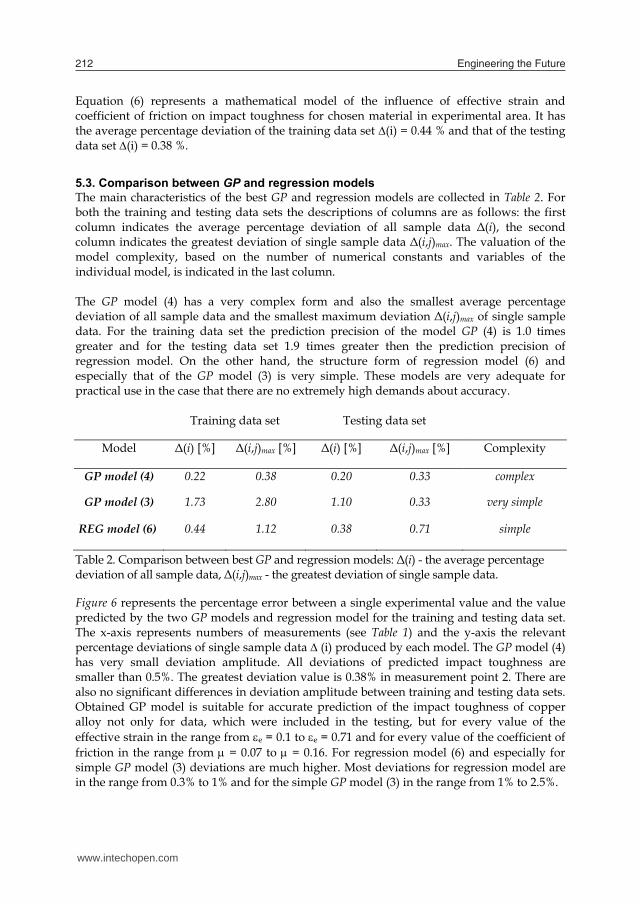
Equation (6) represents a mathematical model of the influence of effective strain and coefficient of friction on impact toughness for chosen material in experimental area. It has the average percentage deviation of the training data set ∆(i) = 0.44 % and that of the testing data set ∆(i) = 0.38 %.
5.3. Comparison between GP and regression models The main characteristics of the best GP and regression models are collected in Table 2. For both the training and testing data sets the descriptions of columns are as follows: the first column indicates the average percentage deviation of all sample data Δ(i), the second column indicates the greatest deviation of single sample data Δ(i,j)max. The valuation of the model complexity, based on the number of numerical constants and variables of the individual model, is indicated in the last column. The GP model (4) has a very complex form and also the smallest average percentage deviation of all sample data and the smallest maximum deviation Δ(i,j)max of single sample data. For the training data set the prediction precision of the model GP (4) is 1.0 times greater and for the testing data set 1.9 times greater then the prediction precision of regression model. On the other hand, the structure form of regression model (6) and especially that of the GP model (3) is very simple. These models are very adequate for practical use in the case that there are no extremely high demands about accuracy.
Training data set Testing data set
Model Δ(i) [%] Δ(i,j)max [%] Δ(i) [%] Δ(i,j)max [%] Complexity
GP model (4) 0.22 0.38 0.20 0.33 complex
GP model (3) 1.73 2.80 1.10 0.33 very simple
REG model (6) 0.44 1.12 0.38 0.71 simple
Table 2. Comparison between best GP and regression models: Δ(i) - the average percentage deviation of all sample data, Δ(i,j)max - the greatest deviation of single sample data. Figure 6 represents the percentage error between a single experimental value and the value predicted by the two GP models and regression model for the training and testing data set. The x-axis represents numbers of measurements (see Table 1) and the y-axis the relevant percentage deviations of single sample data ∆ (i) produced by each model. The GP model (4) has very small deviation amplitude. All deviations of predicted impact toughness are smaller than 0.5%. The greatest deviation value is 0.38% in measurement point 2. There are also no significant differences in deviation amplitude between training and testing data sets. Obtained GP model is suitable for accurate prediction of the impact toughness of copper alloy not only for data, which were included in the testing, but for every value of the effective strain in the range from e = 0.1 to e = 0.71 and for every value of the coefficient of friction in the range from = 0.07 to = 0.16. For regression model (6) and especially for simple GP model (3) deviations are much higher. Most deviations for regression model are in the range from 0.3% to 1% and for the simple GP model (3) in the range from 1% to 2.5%.
Fig. 6. Absolute deviation of model results from the experimental results in a singular measurement point.
6. Conclusion
The presented genetic programming approach for modeling of material properties (in our case impact toughness) strongly differs from the conventional methods since it does not use strict mathematical rules and does not derive equations in a rational human way of thinking. The evolutionary process is non-deterministic and involves asynchronous, uncoordinated, and self-organizing activities that are not centrally controlled. During our research, several different models for impact toughness satisfying the criterion of the success were discovered. The obtained models differ in size, shape, complexity and precision of the solution. The study showed that a GP approach is suitable for system modeling. A comparison was made between GP and regression models. In modeling with the regression method, the form of the prediction models was pre-specified. On the contrary, in modeling with the GP, the form, size, and complexity of the models were left to simulated evolution. The resulting models were tested by the testing data set and compared with respect to different criteria. It is a disadvantage of the GP approach that the modeling lasts longer than in regression approach and that the models are much more complicated. This is due to the fact that evolution is a stochastic process, and therefore parsimony in the development of the models is rare. But in many metal forming processes it is not the model
0
0,5
1
1,5
2
2,5
3
0 2 4 6 8 10 12 14 16 18 20
measurement point
abso
lute
dev
iatio
n [%
] GP model(4)
GP model(3)
REG model(6)
www.intechopen.com

Evolutionary computation method for modeling of material properties 213
Equation (6) represents a mathematical model of the influence of effective strain and coefficient of friction on impact toughness for chosen material in experimental area. It has the average percentage deviation of the training data set ∆(i) = 0.44 % and that of the testing data set ∆(i) = 0.38 %.
5.3. Comparison between GP and regression models The main characteristics of the best GP and regression models are collected in Table 2. For both the training and testing data sets the descriptions of columns are as follows: the first column indicates the average percentage deviation of all sample data Δ(i), the second column indicates the greatest deviation of single sample data Δ(i,j)max. The valuation of the model complexity, based on the number of numerical constants and variables of the individual model, is indicated in the last column. The GP model (4) has a very complex form and also the smallest average percentage deviation of all sample data and the smallest maximum deviation Δ(i,j)max of single sample data. For the training data set the prediction precision of the model GP (4) is 1.0 times greater and for the testing data set 1.9 times greater then the prediction precision of regression model. On the other hand, the structure form of regression model (6) and especially that of the GP model (3) is very simple. These models are very adequate for practical use in the case that there are no extremely high demands about accuracy.
Training data set Testing data set
Model Δ(i) [%] Δ(i,j)max [%] Δ(i) [%] Δ(i,j)max [%] Complexity
GP model (4) 0.22 0.38 0.20 0.33 complex
GP model (3) 1.73 2.80 1.10 0.33 very simple
REG model (6) 0.44 1.12 0.38 0.71 simple
Table 2. Comparison between best GP and regression models: Δ(i) - the average percentage deviation of all sample data, Δ(i,j)max - the greatest deviation of single sample data. Figure 6 represents the percentage error between a single experimental value and the value predicted by the two GP models and regression model for the training and testing data set. The x-axis represents numbers of measurements (see Table 1) and the y-axis the relevant percentage deviations of single sample data ∆ (i) produced by each model. The GP model (4) has very small deviation amplitude. All deviations of predicted impact toughness are smaller than 0.5%. The greatest deviation value is 0.38% in measurement point 2. There are also no significant differences in deviation amplitude between training and testing data sets. Obtained GP model is suitable for accurate prediction of the impact toughness of copper alloy not only for data, which were included in the testing, but for every value of the effective strain in the range from e = 0.1 to e = 0.71 and for every value of the coefficient of friction in the range from = 0.07 to = 0.16. For regression model (6) and especially for simple GP model (3) deviations are much higher. Most deviations for regression model are in the range from 0.3% to 1% and for the simple GP model (3) in the range from 1% to 2.5%.
Fig. 6. Absolute deviation of model results from the experimental results in a singular measurement point.
6. Conclusion
The presented genetic programming approach for modeling of material properties (in our case impact toughness) strongly differs from the conventional methods since it does not use strict mathematical rules and does not derive equations in a rational human way of thinking. The evolutionary process is non-deterministic and involves asynchronous, uncoordinated, and self-organizing activities that are not centrally controlled. During our research, several different models for impact toughness satisfying the criterion of the success were discovered. The obtained models differ in size, shape, complexity and precision of the solution. The study showed that a GP approach is suitable for system modeling. A comparison was made between GP and regression models. In modeling with the regression method, the form of the prediction models was pre-specified. On the contrary, in modeling with the GP, the form, size, and complexity of the models were left to simulated evolution. The resulting models were tested by the testing data set and compared with respect to different criteria. It is a disadvantage of the GP approach that the modeling lasts longer than in regression approach and that the models are much more complicated. This is due to the fact that evolution is a stochastic process, and therefore parsimony in the development of the models is rare. But in many metal forming processes it is not the model
0
0,5
1
1,5
2
2,5
3
0 2 4 6 8 10 12 14 16 18 20
measurement point
abso
lute
dev
iatio
n [%
] GP model(4)
GP model(3)
REG model(6)
www.intechopen.com
Engineering the Future214
complexity but the accuracy of prediction that is of vital importance. However, the best model developed by GP gives a more accurate prediction than the pre-specified model optimised by regression method, due to the fact that in GP a much wider solution space can be analysed since the structure of the models is not prescribed in advance but is left to the evolutionary process. Accuracy of solutions obtained by GP depends on applied evolutionary parameters and also on the number of measurements and the accuracy of measuring. In general, more measurements supply more information to the evolution which improves the structure of models. At the same time, the greater number of measurements causes the time-consuming computer processing and the execution of experiments is very expensive and requires much time. Because of the high precision of the models developed by the GP approach, an excessive number of experiments and computations can be avoided, which leads to reduction of the costs of product development. Because the proposed GP method is general, it can be successfully used for modeling of different materials properties and phenomena where experimental data on the process are available.
References
Barnes, W.(1994). Statistical Analysis for Engineers and Scientists – a computer based approach, The University of Texas at Austin, McGraw – Hill, New York.
Brezocnik M., Kovacic, M., & Gusel, L. (2005). Comparison between genetic algorithm and genetic programming approach for modeling the stress distribution. Materials and Manufacturing Processes, 20, 497 – 508.
Chang, Y.S., Kwang, S.P., & Kim, B.Y. (2005). Nonlinear model for ECG R-R interval variation using genetic programming approach. Future Generation Computer Systems, 21, 1117 – 1123.
Dimitriu, R. C., Bhadeshia, H. K. D. H., Fillon, C., & Poloni,C. (2009). Strength of Ferritic Steels: Neural Networks and Genetic Programming, Materials and Manufacturing Processes, 24/1, 10 – 15.
Fakhrzad, M.B., & Khademi Zare, H. (2009).Combination of genetic algorithm with Lagrange multipliers for lot-size determination in multi-stage production scheduling problems. Expert Systems with Applications, 36 (6),
10180-10187. Koza, J.R. (1992). Genetic programming. (1st ed.). The MIT Press, Massachusetts. Koza, J.R. (1994) Genetic programming II, The MIT Press, Massachusetts. Koza, J.R., Keane, M.A., Streeter, M. J., Mydlowec, W., Yu, J., & Lanza, G. (2003). Genetic
Programming IV: Routine Human - Competitive Machine Intelligence, Kluwer Academic Publishers.
Koza, J.R., Bennett III, F. H., Andre, D., & Keane, M. A. (1999).Genetic Programming III: Darwinian Invention and Problem Solving, Morgan Kaufmann Publishing.
Lange, K. (2001). Handbook of metal forming, McGraw Hill, New York. Mitchell, T.M. (1997). Machine learning, McGraw-Hill, New York. Mohanty, S., Mahanty, B., & Mohapatra, P.K.J. (2003). Optimization of Hot Rolled Coil
Widths Using a Genetic Algorithm. Materials and Manufacturing Processes, 18(3), 447-462.
Mondal, S., & Maiti, M. (2002). Multi-item fuzzy EOQ models using genetic algorithm, Computers & Industrial Engineering 44, 105–117.
Montgomery, D.C., Runger, G.C., & Hubele, N.F. (2001). Engineering statistics. (2nd ed.). New York. John Wiley & Sons.
Odugava, V., Tiwari, A., & Roy, R. (2005). Evolutionary computing in Manufacturing industry: an overview of recent applications, Applied Soft Computing, 5, 281 – 299.
Özel, T., & Karpat, I. (2005). Predictive modeling of surface roughness and tool wear in hard turning using regression and neural networks. International Journal of Machine Tools and Manufacture, 45 (4-5), 467 – 479.
Pierrevall, H., Caux, C., Paris, J.L., & Viguier, F. (2003). Evolutionary approaches to the design and organization of manufacturing system. Computers & Industrial Engineering, 44, 339 – 364.
Sette S., & Boullart, L. (2001). Genetic programming: principles and applications, Engineering Applications of Artificial Intelligence 14, 727 – 736.
Tanguy, B., Besson, J., Piques, R. & Pineau, A. (2005). Ductile to brittle transition of an A508 steel characterized by Charpy impact test – Part 1: experimental results.Engineering Fracture Mechanics, 72, 49 – 72.
www.intechopen.com

Evolutionary computation method for modeling of material properties 215
complexity but the accuracy of prediction that is of vital importance. However, the best model developed by GP gives a more accurate prediction than the pre-specified model optimised by regression method, due to the fact that in GP a much wider solution space can be analysed since the structure of the models is not prescribed in advance but is left to the evolutionary process. Accuracy of solutions obtained by GP depends on applied evolutionary parameters and also on the number of measurements and the accuracy of measuring. In general, more measurements supply more information to the evolution which improves the structure of models. At the same time, the greater number of measurements causes the time-consuming computer processing and the execution of experiments is very expensive and requires much time. Because of the high precision of the models developed by the GP approach, an excessive number of experiments and computations can be avoided, which leads to reduction of the costs of product development. Because the proposed GP method is general, it can be successfully used for modeling of different materials properties and phenomena where experimental data on the process are available.
References
Barnes, W.(1994). Statistical Analysis for Engineers and Scientists – a computer based approach, The University of Texas at Austin, McGraw – Hill, New York.
Brezocnik M., Kovacic, M., & Gusel, L. (2005). Comparison between genetic algorithm and genetic programming approach for modeling the stress distribution. Materials and Manufacturing Processes, 20, 497 – 508.
Chang, Y.S., Kwang, S.P., & Kim, B.Y. (2005). Nonlinear model for ECG R-R interval variation using genetic programming approach. Future Generation Computer Systems, 21, 1117 – 1123.
Dimitriu, R. C., Bhadeshia, H. K. D. H., Fillon, C., & Poloni,C. (2009). Strength of Ferritic Steels: Neural Networks and Genetic Programming, Materials and Manufacturing Processes, 24/1, 10 – 15.
Fakhrzad, M.B., & Khademi Zare, H. (2009).Combination of genetic algorithm with Lagrange multipliers for lot-size determination in multi-stage production scheduling problems. Expert Systems with Applications, 36 (6),
10180-10187. Koza, J.R. (1992). Genetic programming. (1st ed.). The MIT Press, Massachusetts. Koza, J.R. (1994) Genetic programming II, The MIT Press, Massachusetts. Koza, J.R., Keane, M.A., Streeter, M. J., Mydlowec, W., Yu, J., & Lanza, G. (2003). Genetic
Programming IV: Routine Human - Competitive Machine Intelligence, Kluwer Academic Publishers.
Koza, J.R., Bennett III, F. H., Andre, D., & Keane, M. A. (1999).Genetic Programming III: Darwinian Invention and Problem Solving, Morgan Kaufmann Publishing.
Lange, K. (2001). Handbook of metal forming, McGraw Hill, New York. Mitchell, T.M. (1997). Machine learning, McGraw-Hill, New York. Mohanty, S., Mahanty, B., & Mohapatra, P.K.J. (2003). Optimization of Hot Rolled Coil
Widths Using a Genetic Algorithm. Materials and Manufacturing Processes, 18(3), 447-462.
Mondal, S., & Maiti, M. (2002). Multi-item fuzzy EOQ models using genetic algorithm, Computers & Industrial Engineering 44, 105–117.
Montgomery, D.C., Runger, G.C., & Hubele, N.F. (2001). Engineering statistics. (2nd ed.). New York. John Wiley & Sons.
Odugava, V., Tiwari, A., & Roy, R. (2005). Evolutionary computing in Manufacturing industry: an overview of recent applications, Applied Soft Computing, 5, 281 – 299.
Özel, T., & Karpat, I. (2005). Predictive modeling of surface roughness and tool wear in hard turning using regression and neural networks. International Journal of Machine Tools and Manufacture, 45 (4-5), 467 – 479.
Pierrevall, H., Caux, C., Paris, J.L., & Viguier, F. (2003). Evolutionary approaches to the design and organization of manufacturing system. Computers & Industrial Engineering, 44, 339 – 364.
Sette S., & Boullart, L. (2001). Genetic programming: principles and applications, Engineering Applications of Artificial Intelligence 14, 727 – 736.
Tanguy, B., Besson, J., Piques, R. & Pineau, A. (2005). Ductile to brittle transition of an A508 steel characterized by Charpy impact test – Part 1: experimental results.Engineering Fracture Mechanics, 72, 49 – 72.
www.intechopen.com

Engineering the Future216
www.intechopen.com

Engineering the FutureEdited by Laszlo Dudas
ISBN 978-953-307-210-4Hard cover, 414 pagesPublisher SciyoPublished online 02, November, 2010Published in print edition November, 2010
InTech EuropeUniversity Campus STeP Ri Slavka Krautzeka 83/A 51000 Rijeka, Croatia Phone: +385 (51) 770 447 Fax: +385 (51) 686 166www.intechopen.com
InTech ChinaUnit 405, Office Block, Hotel Equatorial Shanghai No.65, Yan An Road (West), Shanghai, 200040, China
Phone: +86-21-62489820 Fax: +86-21-62489821
This book pilots the reader into the future. The first three chapters introduce new materials and materialprocessing methods. Then five chapters present innovative new design directions and solutions. The mainsection of the book contains ten chapters organized around problems and methods of manufacturing andtechnology, from cutting process optimisation through maintenance and control to the Digital Factory. The lasttwo chapters deal with information and energy, as the foundations of a prospering economy.
How to referenceIn order to correctly reference this scholarly work, feel free to copy and paste the following:
Leo Gusel (2010). Evolutionary Computation Method for Modeling of Material Properties, Engineering theFuture, Laszlo Dudas (Ed.), ISBN: 978-953-307-210-4, InTech, Available from:http://www.intechopen.com/books/engineering-the-future/evolutionary-computation-method-for-modeling-of-material-properties

© 2010 The Author(s). Licensee IntechOpen. This chapter is distributedunder the terms of the Creative Commons Attribution-NonCommercial-ShareAlike-3.0 License, which permits use, distribution and reproduction fornon-commercial purposes, provided the original is properly cited andderivative works building on this content are distributed under the samelicense.