totocaca

METALLURGY TRAINING MODULE 9 REV. A01

BY

JDD

DATE

06/03/13 Mechanical Properties

of 73 APPROVED

DATE

Introduction

Apply a stress to a metal and it will deform. Mechanical properties characterize how a metal will react to an applied stress. The deformation that occurs may either be temporary, that is, it will disappear if the stress is removed, or it may be permanent. For example, suppose we place a small, metal rod into a load frame and apply a tensile load. The rod will begin to stretch or increase in length. The volume of material cannot change hence as the rod becomes longer, its diameter must become smaller. Up to a certain point of loading the dimensional changes that occur will be completely reversible. The rod will return back to its original diameter and length if the load is removed. This is known as elastic behavior. If we continue loading beyond this point, some permanent deformation will occur. The rod will still contract slightly in length and increase in diameter if the load is removed, but will not it return all the way to its original dimensions. It has become permanently deformed. This is known as plastic behavior. There are many tests available for characterizing the mechanical properties of metals. In this module we will address the tensile test, impact testing, hardness testing, and fracture toughness testing.

The Tensile Test

The tensile test is one means of characterizing a metal’s mechanical properties in terms of strength and ductility when a tensile load is applied. All of the ARGUS material specifications reference ASTM A370 for the mechanical testing. ASTM A370, in turn, invokes ASTM E8 for tensile testing.

A typical tensile tester consists of a load frame, a movable crosshead, and a pair of specimen grips: one fixed and one attached to the movable crosshead. The movable crosshead can move up and down and is actuated by a hydraulic or electromechanical mechanism. The test specimen is placed in the grips and a device called an extensometer is attached to the specimen. The test specimen will be put in tension (or stretched) as the movable crosshead moves away from the fixed grips. The test specimen will elongate and eventually break as the load continues to increase. The test is finished after the test specimen has fractured in two. The speed that the movable crosshead travels is a critical test parameter and is controlled by ASTM. It may vary during different stages of the test. The load frames used in tensile testing come in many sizes depending on the size and strength of the material that they are designed to test. Those for testing standard size steel specimens as well as full size parts will be large and robust as shown in Figure 1. A medium duty frame is shown in Figures 2. Metals aren’t the only things that are tensile tested. A light duty frame may be used to test the tensile properties of fabrics,


BY

JDD

DATE


of 73 APPROVED

DATE

plastics, and elastomers. These materials are often tested in a table top model of tensile tester as shown in Figure 3.

Figure 1: Heavy Duty Load Frame (Photo Courtesy of Ron Richter, Houston

Metallurgy Laboratory, Inc.)

Figure 2: Medium Duty Load Frame ( Photo Courtesy of Ron Richter, Houston



BY

JDD

DATE


of 73 APPROVED

DATE

Figure 3: Light Duty Load Frame (Photo Courtesy of Ron Richter, Houston


There are two basic measurements made during a tensile test: the load that the test specimen is subject to at any given moment of time, and the corresponding elongation or displacement (stretching) of the test specimen. The load is continuously measured by a load cell attached to the fixed grip in the tensile tester, while the elongation is measured by the extensometer that was clipped on the test specimen (see Figure 4 for an example). The extensometer sends out an electrical signal proportional to the amount of movement that occurs between its two arms that are in contact with the test specimen. The outputs from the load cell and extensometer are digitally recorded on modern test machines and may also be recorded on an X-Y plotter. The extensometer is removed before the specimen fractures to prevent it from being damaged.

There are many types of tensile test specimens. The two basic types for steel products are round and flat specimens (see Figure 5). Both come in a number of standard sizes as prescribed by ASTM. There are many ways to affix the ends of a tensile specimen in the load frame so ASTM does not cover the configuration of the ends of the test specimens. Test specimens may have threaded ends, button head ends, etc. A round specimen will be turned so that it has a reduced cross section in the middle section of the specimen. The purpose of this is to ensure that fracture occurs in the approximate middle of the test specimen and not in the gripped ends. This reduced cross section is called the gage diameter. ASTM specifies a nominal gage diameter of 0.500” for a full


BY

JDD

DATE


of 73 APPROVED

DATE

size round specimen. ASTM also prescribes the minimum length of this reduced section. Flat tensile test specimens are typically used for flat, rolled products or for thin wall pipe. The ends of a flat specimen are considerably wider than the center section giving them a dumbbell shape (flat specimens are often referred to as “dog bone” specimens because of their shape). The thickness of the flat specimen is usually the thickness of the flat product or the wall thickness of the pipe from which it was removed.

Figure 4: Example of a Contact Extensometer

Figure 5: Tensile Test Specimens (From Wikipedia,

http://en.wikipedia.org/wiki/Tensile_testing)


BY

JDD

DATE


of 73 APPROVED

DATE

After the test specimen (either round or flat) has been machined, the reduced section of the specimen is marked with a steel punch that leaves two small indentations. The distance between the two points is called the gage length. It is an arbitrary distance specified by ASTM that serves as a reference in our calculations and interpretations of the test results. A gage length for a full size round specimen is 2” while that of a full size flat specimen is 8”.

The values of load versus elongation obtained during the test are used to develop an engineering stress-strain curve. The load - elongation curve and the engineering stress-strain curve have the same shape and differ only in units. A typical engineering stress – strain curve for a ductile steel is shown in Figure 6. Engineering stress is defined as the load at any given point in time divided by the original cross sectional area of the test specimen’s gage diameter section. It has units of pounds force per square inch or psi. Strain is the amount of elongation that occurs per unit of length at any given moment of time. It is expressed as a percentage or in inches/inch. A lot of useful information can be obtained from an engineering stress-strain curve. We’ll examine the key points.

Figure 6: Engineering Stress-Strain Curve Typical For A Ductile Steel


BY

JDD

DATE


of 73 APPROVED

DATE

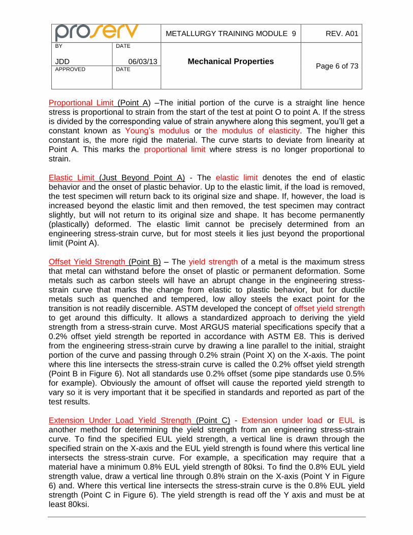
Proportional Limit (Point A) –The initial portion of the curve is a straight line hence stress is proportional to strain from the start of the test at point O to point A. If the stress is divided by the corresponding value of strain anywhere along this segment, you’ll get a constant known as Young’s modulus or the modulus of elasticity. The higher this constant is, the more rigid the material. The curve starts to deviate from linearity at Point A. This marks the proportional limit where stress is no longer proportional to strain.

Elastic Limit (Just Beyond Point A) - The elastic limit denotes the end of elastic behavior and the onset of plastic behavior. Up to the elastic limit, if the load is removed, the test specimen will return back to its original size and shape. If, however, the load is increased beyond the elastic limit and then removed, the test specimen may contract slightly, but will not return to its original size and shape. It has become permanently (plastically) deformed. The elastic limit cannot be precisely determined from an engineering stress-strain curve, but for most steels it lies just beyond the proportional limit (Point A).

Offset Yield Strength (Point B) – The yield strength of a metal is the maximum stress that metal can withstand before the onset of plastic or permanent deformation. Some metals such as carbon steels will have an abrupt change in the engineering stress-strain curve that marks the change from elastic to plastic behavior, but for ductile metals such as quenched and tempered, low alloy steels the exact point for the transition is not readily discernible. ASTM developed the concept of offset yield strength to get around this difficulty. It allows a standardized approach to deriving the yield strength from a stress-strain curve. Most ARGUS material specifications specify that a 0.2% offset yield strength be reported in accordance with ASTM E8. This is derived from the engineering stress-strain curve by drawing a line parallel to the initial, straight portion of the curve and passing through 0.2% strain (Point X) on the X-axis. The point where this line intersects the stress-strain curve is called the 0.2% offset yield strength (Point B in Figure 6). Not all standards use 0.2% offset (some pipe standards use 0.5% for example). Obviously the amount of offset will cause the reported yield strength to vary so it is very important that it be specified in standards and reported as part of the test results. Extension Under Load Yield Strength (Point C) - Extension under load or EUL is another method for determining the yield strength from an engineering stress-strain curve. To find the specified EUL yield strength, a vertical line is drawn through the specified strain on the X-axis and the EUL yield strength is found where this vertical line intersects the stress-strain curve. For example, a specification may require that a material have a minimum 0.8% EUL yield strength of 80ksi. To find the 0.8% EUL yield strength value, draw a vertical line through 0.8% strain on the X-axis (Point Y in Figure 6) and. Where this vertical line intersects the stress-strain curve is the 0.8% EUL yield strength (Point C in Figure 6). The yield strength is read off the Y axis and must be at least 80ksi.


BY

JDD

DATE


of 73 APPROVED

DATE

Curve Segment C to D - Plastic deformation is uniform along this part of the curve. The diameter along the gage length will uniformly contract as the specimen elongates (the volume must remain the same!). Ultimate Tensile Strength (Point D) - The ultimate tensile strength or just tensile strength is the highest point on the engineering stress-strain curve. It defines the highest load or stress that the metal can withstand before breaking. Curve Segment D to Fracture – The load necessary to cause a given amount of strain begins to lessen after the tensile strength of the metal has been reached because the test specimen no longer has uniform deformation. There will some point along the gage length where localized deformation will be much greater than other points due to inhomogeneities of the cross-sectional area or the local work-hardening rate. This causes an abrupt change in diameter (see Figure 7) referred to as “necking”. As the specimen necks down in diameter, the curve will begin to drop. Necking will continue until fracture occurs and the specimen breaks into two halves.

Figure 7: Necking In A Tensile Specimen

After the test is completed, we will have to take some measurements from the broken test specimen. The size and shape of the specimen have changed during the test. If the broken halves are fitted together, we’ll see that the overall length has increased while the diameter of the gage length section has decreased especially in that portion where necking occurred. The distance between the punch marks used to denote the gage


BY

JDD

DATE


of 73 APPROVED

DATE

length has become greater. The percent increase in gage length that occurs during the test is called percent elongation. It is found using the following formula:

%El = L final –L original X 100% Where %El = percent elongation L original L = distance between gage length punch marks

It is apparent from the formula why it is important to specify the desired gage length in a material specification as well as when reporting the percent elongation results. The original gage length is the reference distance against which we will compare the final distance between the punch marks. The calculated value of %El for a given specimen after testing will vary depending upon the original gage length. The test specimen volume doesn’t change during the test. Material is rearranged, but none is lost. If the length of the specimen elongates, then the diameter must contract. The percent decrease in cross sectional area that occurs when the initial gage diameter is reduced to the smallest diameter at the point of fracture is called percent reduction of area. It is found by the following formula: %RA = A final – A original X100% where %RA = percent reduction of area

A original A = area based upon the gage diameter

Note that the reduction of area cannot be calculated for flat tensile test specimens because of their rectangular cross sections.

Ductility is the metal’s ability to undergo plastic deformation under a tensile load without cracking or fracturing. Minimum values of elongation and reduction of area are prescribed in material specifications to insure adequate ductility. The greater the ductility, the harder it will be for a crack to initiate and grow. Even though the average bulk stresses on a metal part may be well below its yield strength, localized stresses at a stress riser such as a notch or a machine mark may easily exceed its yield strength. This can lead to rapid crack initiation and growth and result in brittle fracture. A ductile metal, on the other hand, will be able to plastically deform without cracking thus redistributing and lowering the stresses at the stress riser to below the yield strength. As a metal’s yield and tensile strengths increase, the percent elongation and reduction of area go down. Maximizing strength will minimize ductility and vice versa. Compromises must always be made. Microcleanliness has an important influence on a metal’s ductility: the cleaner the steel, the better its ductility. Small inclusion act as stress risers that can initiate microcracking.


BY

JDD

DATE


of 73 APPROVED

DATE

The yield and ultimate tensile strength of a metal both will vary by test temperature (decreasing as temperature increases). Material specifications for parts destined for high temperature service will frequently specify that elevated temperature tensile tests be run. To run a high temperature test, a longer than normal test specimen may be used (still with a standard gage length). The specimen is placed in the grips of the tensile tester and a small, electric clamshell furnace is placed around it. When the specimen reaches the test temperature, the clamshell furnace is removed, an extensometer clipped on the specimen, and then the test started. High temperature tensile testing requires special equipment and not all labs can do it. These issues can be avoided by using a material specification that requires only a room temperature tensile test, but imposes a higher minimum yield strength than that required at room temperature to allow for the drop that will occur at service temperatures. As a given steel is heat treated to higher strength levels, the yield strength will begin to approach the value of the ultimate tensile strength. The yield must not be allowed to become too close to the ultimate tensile strength or else there will be little room for plastic deformation to occur to redistribute stresses at stress risers and prevent rapid, brittle fracture. Many high strength steel specifications will specify a maximum yield strength/ultimate tensile strength ratio (often 0.9 or so) to insure that some plastic deformation can occur before fracture. The orientation of a tensile specimen in forged material is not particularly important unless the material has poor hardenability. Transverse or longitudinal specimens should have approximately the same strength levels, although % elongation and reduction of area may be slightly lower in a transverse specimen. Most specifications allow either orientation as convenient. Only one test is typically run, but occasionally several tests may be required if a part has several different critical areas that need to be examined. Tensile testing pipe presents several special problems. Heavy wall pipe may not have uniform tensile properties throughout its wall. Heavy wall, seamless pipe, for example, will typically have better properties near the OD than the ID because the OD gets a more effective quench during heat treating. A dog bone (flat) specimen may give results that are more representative of the overall properties of the pipe than a round specimen in this case. The dog bone specimen encompasses the entire wall thickness of the pipe. A round specimen may have a gage diameter much smaller than the pipe wall section so results may vary depending on where the specimen is removed. Pipe made from rolled and welded plate should have very uniform properties throughout the wall. Some pipe specifications require that tensile specimens be taken in a circumferential orientation (transverse to the longitudinal axis of the pipe). Usually either a round tensile specimen or a full cross section, dog bone specimen is permitted. A dog bone specimen blank removed in a transverse orientation from a large pipe will obviously have to be flattened to get rid of the curvature before tensile testing. Flattening the


BY

JDD

DATE


of 73 APPROVED

DATE

specimen prior to testing will induce some new, plastic strains that may alter the resulting yield strength during the tensile test. This is known as the Bauschinger effect.

As a result of the Bauschinger effect, metal plastically deformed will see an increase in yield strength in the direction of plastic flow, but a reduction in yield strength in other directions. A transverse tensile blank removed from a large diameter pipe will be curved somewhat like a banana. The OD surface will be strained in compression and the ID in tension during the flattening process. The final strain pattern in the flattened metal will be very complex. The magnitude and orientation of the imparted strains is highly dependent on how the flattening process is done. In most cases there will be a decrease (up to 10% or so!) in the yield strength of the flattened tensile specimen in comparison to the actual yield strength of the pipe. The Bauschinger effect can be minimized by flattening in small increments along the length of the tensile blank rather than flatten the entire specimen all between two platens. Pipe mills are thoroughly familiar with this effect, but some commercial labs are not. If you ever have to retest pipe at a commercial lab using transverse specimens and the yield strength results vary significantly from what the mill reported on the MTR, then check on how the lab flattened the specimen. You can have the lab run a longitudinal specimen for comparison. The longitudinal specimen does not require flattening. The yield strengths in both orientations should be approximately the same.

The use of turned (round), transverse tensile specimens avoids the problem of flattening and the Bauschinger effect, but now another problem arises. In a heavy wall, seamless pipe, the gage section of the turned specimen will be closest (tangent) to the ID surface while the ends of the specimen will be nearer the OD due to geometry constraints. The material near the ID surface often has the poorest properties. The advantage of a dog bone when the tensile specimen must be taken in a transverse orientation is that it can be full section size and thus take advantage of the stronger material on the OD.

The Impact Test

The purpose of a Charpy V-notch impact test is to determine the notch toughness of a metal. Notch toughness is the energy it takes to initiate and propagate a crack in a prescribed metal specimen that contains a stress riser in the form of a notch. The notch toughness of a metal varies with strength level, microstructure, test specimen configuration, orientation of the test specimen to the direction of greatest hot working in the metal, and testing parameters. Toughness is an important property in a metal because the higher a metal’s toughness, the harder it is for a crack to initiate and grow, and the less likely the metal will fail by rapid, brittle fracture. There are many standards for Charpy impact testing. ARGUS material specifications invoke ASTM A370 for mechanical testing. ASTM A370 in turn references ASTM E23 for impact testing.


BY

JDD

DATE


of 73 APPROVED

DATE

A standard ASTM E23 Charpy V-notch impact specimen is illustrated in Figure 8. The “V” refers to the shape of the small notch that is milled or broached into one side of the specimen. The root of the notch acts as a stress riser where a crack will initiate during the test. Specimen preparation must be done with care in order to obtain accurate and consistent test results. The notch dimensions and tolerances are tightly controlled by ASTM. Any small machining mark or variation in the radius at the notch tip can significantly change results. Notches should always be checked on an optical comparator or using a gage to insure that they have the exact radius. If the part to be impact tested is too small to obtain a full size Charpy specimen (such as a thin wall pipe), then ASTM allows the next smaller subsize specimen to be used instead. A subsize specimen will be thinner (less material under the notch) than a standard size specimen. A reduction factor must be applied to the acceptance criteria specified for a full size specimen. Most material specifications require a minimum of three specimens be tested and the results averaged due to the inherent scatter of the test. Often a minimum average is specified with a stipulation that no single value be below a certain minimum.

Figure 8: Standard SizeASTM Charpy V-Notch Test Specimen Dimensions (mm)

A typical impact tester consists of a rigid base and column securely bolted to the floor, a free swinging pendulum arm, and a cradle or anvil at the bottom to hold the test specimen (see Figure 9). The arm is weighted and has a vertical striking edge on the free swinging end. The arm is raised to the upright position where it latched in place and the dial indicator on top of the column is zeroed. The specimen to be tested is placed in a cradle (also called an “anvil”) at the bottom of the tester such that the cradle supports just the ends of the test specimen and allows the striking edge of the arm to freely pass through. The test specimen is held in the horizontal position, perpendicular to the arc of the swinging pendulum. The side of the specimen with the V-notch is placed directly opposite the side that will be struck by the pendulum (see Figure 10). Once the specimen is properly positioned, the pendulum arm will be released by tripping the latch. The arm will swing down and strike the specimen. The amount of energy absorbed by the test specimen is read off the dial indicator on top of the column.


BY

JDD

DATE


of 73 APPROVED

DATE

At the start of the test, the pendulum arm is fully raised and locked into position thus it has potential energy due to its weight and height, but no kinetic energy. When the latch is released, the pendulum swings down and the potential energy is converted into kinetic energy. At the bottom of its path, all of the potential energy has been converted to kinetic energy. If we allow the pendulum to freely swing (i.e. there is no test specimen in the cradle), the pendulum will begin to swing back upwards on the opposite side now converting kinetic energy back into potential energy. The pendulum will swing back up to its original height (ignoring minor energy losses due to friction of the bearing). The dial indicator will show 0 – there is no energy loss.

Figure 9: Impact Tester (From the National Institute for Standards and Testing)


BY

JDD

DATE


of 73 APPROVED

DATE

Figure 10: Orientation of Notch

Now let’s see what happens when a test specimen is in the cradle. After the latch is tripped, the pendulum arm swings down and strikes the specimen on the side opposite of the notch and breaks it in two. The pendulum will continue its swing after breaking the specimen and will start to rise on the other side, but this time its final height will be lower than its release height. Some of the kinetic energy that the pendulum had at the bottom of its swing was absorbed by the test specimen as it fractured so there’s now less kinetic energy to convert back into potential energy. The pendulum is always released from the same height at the start of the test so will always strike the test specimen with same kinetic energy. The difference between the release height and the final height multiplied by the weight of the pendulum’s striking head will give the amount of energy lost or absorbed by the test specimen. The energy loss is read directly from the dial indicator on top of the column. It is usually reported in ft-lbs (or joules in metric). A tough metal will absorb more energy than a brittle metal when impact tested. The term “impact strength” is occasionally seen in specifications, but this is incorrect - toughness is measured in terms of energy and not a stress. Toughness of a particular steel bar varies with orientation of the test specimen, test temperature, the strength of the material, and the microstructure. The toughness of a wrought material such as rolled or forged bar will vary with how the test specimen is oriented to the direction of greatest hot work. For a bar, the direction of greatest hot work is always along the longitudinal axis of the bar. The grains of metal will elongate and align themselves in the direction of greatest hot work. A longitudinal impact test specimen will be removed from a bar such that its longitudinal axis is parallel to the axis of the bar – the direction of greatest hot work. The notch in the test specimen will then be perpendicular to the bar axis. This will produce the highest toughness because a propagating crack will have to traverse a greater number of grain boundaries in this orientation. Grain boundaries help to strengthen and toughen the material. A transverse impact test specimen is taken with its longitudinal axis perpendicular to the bar axis (that is, in a radial or circumferential direction). A propagating crack will have fewer grain boundaries grain boundaries to cross in a transverse specimen consequently the toughness will be lower. A material specification requiring impact testing must always specify the orientation of the test specimens. Typically the acceptance criteria for longitudinal specimens will be higher than that for transverse specimens. If a material specification calls for a certain minimum impact value when testing is done in the longitudinal orientation, it is generally acceptable to accept transverse results as long as they meet the specified criteria because the transverse orientation is a worst case. If a material specification calls for a certain minimum impact value in the transverse orientation, you cannot accept longitudinal results regardless of their values. ASTM E1823 gives the nomenclature for specifying the orientation of test specimens. Orientation is specified by a two letter code. The first letter gives the orientation of the longitudinal axis of the test specimen in relation to the direction of greatest working. The


BY

JDD

DATE


of 73 APPROVED

DATE

second letter gives the direction that the crack initiating at the V-notch root will propagate in. The nomenclature for a rolled bar is illustrated in Figure 11. Nomenclature

may vary with other product forms. R - Radial L – Longitudinal C - Circumferential Note: If the disk shown is off a bar, then C-R, R-C, C-L, and R-L would all be considered transverse impact specimens.

Figure 11: Orientation Nomenclature for Rolled Bar (From ASTM E1823)

The impact toughness of many metals, especially ferritic metals such as quenched and tempered steels, may vary significantly with test temperature. Most API and other design standards require that material be impact tested at or below the minimum design temperature to insure adequate toughness. Test specimens are cooled down in a bath (the bath may be water and/or acetone with ice or dry ice as needed, or liquid nitrogen, chilling gas, etc.) until the specimen temperature stabilizes at the test temperature. ASTM requires at least 5 minutes in the bath when liquids are used. A pair of tongs is used to transport the specimen from the bath to the test cradle. The specimen handling end of the tongs is kept in the bath with the specimens so it does not affect the temperature of the specimen as it is removed from the bath. The test specimen is removed from the bath using the tongs and immediately placed on the test anvil such that the root of the V-notch is in the vertical position and the notch itself is opposite from the direction that the pendulum will strike from. The latch holding the pendulum in place is then released and the pendulum begins its swing. ASTM requires that the latch must be released within 5 seconds after the specimen has been removed from the bath. The toughness of the broken test specimen is read directly from the dial indicator or digital readout. The variation of a given metal’s toughness with temperature is often illustrated by a Charpy impact transition curve. A transition curve is made by testing a large number of specimens at different test temperatures and then plotting the results. A typical curve for a quenched and tempered, low alloy steel will look like Figure 12. There are several important things to note in Figure 12. First is that as the test temperature decreases eventually a point is reached where the toughness bottoms out to a minimum value. Decreasing the test temperature further will not alter the absorbed energy. This area of


BY

JDD

DATE


of 73 APPROVED

DATE

the curve is known as the lower shelf. Fracture is 100% brittle on the lower shelf – a worst case. Similarly there is a maximum toughness value that will be obtained with increasing test temperature. This maximum is indicative of 100% ductile fracture – a best case. Once we have attained this maximum, increasing the test temperature even further will not increase the absorbed energy. The portion of the curve where absorbed energy is at a maximum is called the upper shelf. The area between the upper and lower shelves is called the transition area. Note that a few degrees may make a big difference in toughness within the transition area. Because absorbed energy varies with temperature, material specifications that require impact testing must specify a test temperature. The test temperature is always at or below the minimum design or service temperature of the part being made from the material. Depending on the material and/or application, some customers may specify a test temperature equal to the minimum service temperature minus 10F or more just to be conservative. From the shape of the curve in Figure 11, it can be seen that if the absorbed energy at test temperature T

o is equal to X ft-lbs, then the absorbed energy at

To + ∆ T

o (any higher temperature higher than T

o) will also be equal to or exceed X ft-

lbs. Test temperatures are thus typically given as maximums. It is generally permissible to test either at or lower than the specified temperature as long as the specified acceptance criteria are met. It is never permissible to test at higher than the specified test temperature. For example, if a spec requires 45ft-lbs minimum at 0

oF, you could

accept a material cert that reports 50 ft-lbs at -50oF, but not one that has 215ft-lbs at

10oF.


BY

JDD

DATE


of 73 APPROVED

DATE

Figure 12: Charpy Impact Transition Curve There are two other pieces of information we can obtain from an individual Charpy test besides the absorbed energy: the percent ductile or fibrous fracture, and the lateral expansion. These are determined from the broken test specimen after the test has been run. The fracture surface of a broken Charpy specimen may appear shiny, dull, or have areas of both. The shiny area is the result of brittle or cleavage fracture where little energy is absorbed. A dull, sooty colored surface is indicative of a ductile or shear failure where a lot of energy is absorbed. The percent of the surface that failed in a ductile mode can quickly be estimated by comparing the broken end of the Charpy specimen to a series of reference photographs in ASTM E23. Material specifications for bars and forgings typically do not require a minimum value for the percent shear or ductile fracture, although they may require it to be reported for information. Carbon steel pipe specifications used in the natural gas transportation industry, however, often require a specified minimum of 50% ductile fracture to insure a predominately ductile failure mode. When the striking edge of the pendulum hits the test specimen in the cradle, the side of the impact specimen that is struck will flare out. The overall increase in the width of the struck side of the specimen is called lateral expansion or LE. It can be quickly measured by running the broken specimen halves along a gage with a dial indicator as shown in Figure 13. It is typically reported in mils (thousandths of an inch). Lateral


BY

JDD

DATE


of 73 APPROVED

DATE

expansion is another measure of the ductility of a fracture. It is generally reported for information only. At one time API 6A had a minimum LE requirement of 15 mils for PSL 4 pressure containing parts, but this requirement has been removed from the standard.

Figure 13: Lateral Expansion Gage

Figure 14 shows a series of Charpy v-notch impact specimens that progress from 100% ductile fracture on the left side of the figure to 100% brittle fracture on the right side. Note the sooty gray appearance as well as the large amount of plastic deformation on the ductile fracture faces on the left side of the figure. The brittle fracture faces on the right show little deformation. They have a shiny, granular appearance. The first two sets of ductile specimens on the left clearly show the flaring that occurred on the side opposite the notch, while the brittle specimens show no discernible flaring thus the ductile specimens have a much greater lateral expansion.


BY

JDD

DATE


of 73 APPROVED

DATE

Figure 14: Broken CVN Impact Specimens Showing Lateral Expansion & Ductile

Fracture (Photo Courtesy of Ron Richter, Houston Metallurgy Laboratory, Inc.)

The absorbed energy of an impact specimen generally varies inversely with strength. The higher the strength that a metal is heat treated to, the lower its impact energy will be. Impact energy is also be a function of the microstructure of the metal. A small grain size will result in higher toughness. A microstructure with more rounded features will typically be tougher than a microstructure with coarse, sharp features that can act as stress risers. Microcleanliness is an important parameter in determining the toughness of a metal: the cleaner the steel, the better the toughness. Inclusions act as stress risers where cracks can initiate. The impact properties of a metal part large bar can vary significantly from surface to mid-wall to center because of the changes in strength, microstructure, and grain size due to the limits in hardenability of the alloy and variation in hot work. Material specifications must thus specify exactly where test specimens are to be taken because results will vary depending on location. The impact test acceptance criteria given in a specification is a somewhat arbitrary number. It is not an inherent material property like tensile or yield strength because it varies with the size of the test specimen. Engineers do not design using an impact value as they would with a tensile or yield strength. Very often the acceptance criteria for a given material (such as in API 6A) is based upon a level of toughness found in parts that have a good track record in service. What constitutes a tough metal? There is no one answer to this because it depends on the metal and how it was processed. An impact value of 15 ft-lbs at 0

oF would be a very low toughness for 4140 low alloy steel

heat treated to 75ksi yield strength, yet it would be an outstanding value for 4140 heat treated to 150ksi yield strength. A Stellite™ having an impact value 2 ft-lbs at 0

oF would

have outstanding toughness. The acceptance criteria specified should reflect the toughness needed for the part in service as well as what toughness would reflect proper processing for a given metal heat treated to the required minimum strength. Because


BY

JDD

DATE


of 73 APPROVED

DATE

an impact value is highly dependent on the material being properly processed (sufficient hot work, proper grain size, good microcleanliness, correct heat treatment, etc.), impact testing is a very effective quality control tool for verifying correct processing. Many specifications for CRA’s (especially for duplex stainless steels and age hardenable nickel based alloys such as 718) require impact values higher than those for low alloy steels or higher than the minimum values specified by design standards such as API 6A. This insures that the CRA’s are correctly processed.

Introduction to Hardness Testing

Hardness is a measure of a metal’s ability to resist penetration of its surface. The surface hardness of a metal is an important factor in determining its resistance to wear, abrasion, and galling. The hardness of a metal can be correlated to its strength if the metal’s heat treat condition is known. The susceptibility of metals to stress corrosion cracking in certain environments is often a function of the metal’s hardness. Hardness testing is a powerful quality control tool to verify that a metal part was processed correctly. Clearly a thorough understanding of hardness is important!

Tensile and impact testing are destructive tests. Test specimens are destroyed during the test and are no longer of any use. We can destructively test a QTC (Qualification Test Coupon) such as a prolongation on a production part, a sacrificial part, or a separately forged test bar, but we cannot tensile or impact test an actual production part without destroying its usefulness. Hardness, on the other hand, is a non-destructive test. The hardness of a metal part can be determined without impairing its subsequent usefulness. In comparison to other mechanical property tests, hardness testing is fast, easy to perform, inexpensive, and non-destructive.

Hardness testing is often the only mechanical test performed on a production part. Only one bar in a heat treat lot of 20 may have a prolongation cut off and be tensile and Charpy V-notch impact tested. The prolongation is wasted material and testing is expensive. It is assumed that the properties obtained are representative of the other bars in the lot. How do we know this is a good assumption? All of the bars in the lot will typically be hardness tested. If the resulting hardness values all fall within the allowable hardness range specified in the applicable material specification, then it is assumed that all the bars were correctly processed and have the necessary mechanical properties similar to those reported for the sacrificial prolongation. Hardness testing of production parts is for acceptance so it must be done correctly. A single hardness value out of range can cause the rejection of a part worth thousands of dollars. We need to have confidence that the surface preparation was done correctly, the indentation was properly made, that the hardness value was accurately read, and that the resulting


BY

JDD

DATE


of 73 APPROVED

DATE

hardness is indeed a true reflection of the hardness of the part before rejecting or accepting a part! The person performing or evaluating a hardness test needs to have a basic understanding of metallurgy in order to avoid pitfalls and errors. Let’s review some of the things we covered previously in the modules on Basic Metallurgy and Heat Treating that pertain to hardness testing. Low alloy steels used in our products are typically austenitized, quenched, and tempered. The austenitizing step consists of heating the steel up to a high temperature (typically 1550-1650F) and holding it until it becomes homogenized and develops a completely austenitic (FCC) crystal structure. The steel is then immersed or quenched in a fluid to cool it as rapidly as possible without cracking it. The austenite will transform into several possible products as it is cooled down depending on the cooling rate. In order of increasing hardness, these transformation products include ferrite, pearlite, bainite, and martensite. Bainite and martensite will only form if a critical cooling rate is exceeded during quenching. The as-quenched steel is very strong and hard, but also very brittle. To restore some of the ductility and toughness, it is tempered. The tempering temperature is selected to produce the desired mechanical properties (typically somewhere between 900-1350F for low alloy steels). This is well below the austenitizing range. The steel is held at the tempering temperature until the desired properties are obtained. Tempering reduces the strength and hardness, but will greatly improve ductility and toughness.

The hardness properties of a steel bar are dependent on its composition, the specific heat treatment, and the size (cross section) of the part at the time of heat treatment. The hardenability of a steel is a measure of how easy it is to attain a given hardness or other mechanical properties at a specific location within its cross section during heat treatment. Steel is essentially an alloy of iron and carbon. As the amount of carbon increases, so does the strength and hardness of the steel for a given heat treatment. 4130. 4140, and 4145 are all members of the Cr-Mo low alloy steel family (the 41XX series). They differ primarily in carbon content (the last two digits in the number represent their nominal carbon content in hundredths of a per cent). Thus 4130 has a nominal carbon content of 0.30%, 4140 has 0.40% nominal carbon, and 4145 has 0.45% nominal carbon. 4145 will have a higher as-quenched hardness than the 4130 because of the higher carbon content in 4145. Similarly, if one heat of 4130 has an actual carbon content of 0.28% and another heat of 4130 has a 0.32% carbon content and they are both heat treated together in the same furnace load, you would expect the heat with 0.32% carbon to be stronger and harder after heat treatment.

The carbon content of a heat of steel is fixed once it’s melted and solidified, however, the surface carbon content of a steel part can change during hot working or during annealing or austenitizing through a process called decarburization. Carbon at the surface of the steel can react with oxygen in the air to form carbon monoxide gas which is then lost to the atmosphere. This leaves a carbon depleted zone on the surface of the metal about 1/16” thick that will be much softer than the underlying metal. This


BY

JDD

DATE


of 73 APPROVED

DATE

decarb layer, as it is called, must be removed during surface preparation in order to obtain an accurate bulk hardness. Steels have many different alloying elements added for varying reasons. Elements such as manganese, chromium, nickel, molybdenum, vanadium, and columbium are added to increase the hardenability of the steel. These elements make it easier to meet the required properties in heavy cross sections by reducing the critical cooling rate necessary for bainite and martensite formation. The higher the content of these alloying elements, the greater the hardenability of the steel will be resulting better hardness uniformity. The specific heat treat parameters obviously will have a profound effect on the hardness of the steel. The as-quenched hardness is primarily a function of the composition of the steel and how rapidly it is quenched. The hardness of the steel following the temper is dependent on tempering time and temperature. The higher the tempering temperature, the softer the metal will become. The longer the holding time at a given tempering temperature, the softer the metal will become. The size at the time of heat treatment affects the hardness of a low alloy steel part. There is a certain critical rate that must be exceeded in order to get the desired change in crystal structure. The faster part can be cooled after austenitizing, the higher the resulting hardness will be and the greater the depth of hardening.

Consider a 1” diameter bar and a 12” diameter bar of 4130 low alloy steel. We’ll austenitize both at 1625F, water quench, and then temper both at 1250F. If we then take a transverse slice through the middle of each bar and make a hardness traverse across a diameter, how will the hardnesses compare? The surface hardness of the 1” bar will be higher than that of the 12” bar because it cools more rapidly during the quench. The second thing to notice is that the hardness throughout the cross section of the1” bar is uniform, while there is a significant drop in hardness as you get below the surface of the 12” bar. The reason for this behavior is obvious. The 1” bar can be cooled much more rapidly during the water quench than the 12” bar. The 1” bar in our example has uniform properties throughout its cross section because the surface and the center cool at approximately the same rate. This is not true for the 12” bar where the center will cool at a much slower rate than the surface. There may be a point below the surface in the 12” bar where the cooling rate falls below the critical rate and no hardening will occur. If we can’t cool a large bar fast enough to get the desired properties where we need them, we must either change the steel to another grade with higher hardenability or we can preheat treat machine the bar. If we can rough out the part to be made from the bar prior to heat treating, we may remove enough material to significantly improve the cooling rate during quenching and hence improve the properties. Often preheat treat machining a simple bore is sufficient.

The bottom line of this discussion is that the surface hardness of an autenitized, quenched, and tempered low alloy steel will always be harder than the center hardness. As you go below the surface, the cooling rate during quenching drops off and hardness


BY

JDD

DATE


of 73 APPROVED

DATE

will decrease until it reaches a minimum at the center. Steels always behave like this – it’s the nature of the beast. If your hardness values don’t show this, then there’s something wrong with the way you are doing the surface preparation, your test set-up, or how you’re reading the results!

The surface hardness of metals may be increased mechanically through work hardening, cold straightening, cold rolling, etc. All of these impart high residual stresses in the metal that strengthen and harden the surface. The hardness of a work hardened metal may be considerably higher than the bulk hardness developed during heat treatment. The hardness increase due to work hardening can be removed by stress relieving..

Hardness Acceptance Criteria

An inspector performing a hardness test on a part in the shop will evaluate the results against the required hardness range in the applicable material specification. How were the minimum and maximum values in the material spec established? A rough correlation between a metal’s hardness and its tensile and yield strengths can be made provided the heat treatment is known. The minimum acceptable value of the specified hardness range is generally based upon the minimum specified yield strength of the metal in the specified heat treated condition. In some cases a slightly higher hardness value may be selected to be conservative. The maximum acceptable hardness of the specified range can be based on several different parameters. It may be based on the highest allowed strength level in the metal that still has adequate ductility and toughness for a given application. As hardness increases in a metal with a given type of heat treatment, strength increases, but toughness and ductility decrease. To get the required ductility and toughness, the hardness and strength must have an upper limit. Many metals are subject to stress corrosion cracking in certain environments if they exceed a certain strength or hardness. Thus a maximum hardness may be based a threshold hardness limit below which stress corrosion cracking in service will not occur. A good example of this is 22 HRC hardness limit imposed by NACE MR0175/ISO 15156 for low alloy steels used in oilfield applications that may be exposed to H2S. The rough correlation between hardness and the tensile and yield strengths of a metal only holds true if the metal’s heat treatment is known. What if you have a part no pedigree? If the hardness falls within range can we assume that the tensile and yield strength are also acceptable? No we cannot. For example, a 4” bar of normalized 4140 has a surface hardness around 241 HBW. The same bar can be austenitized, quenched, and tempered to exactly the same surface hardness. The tensile strengths in both bars will be approximately the same – about 115 ksi. The yield strengths, however, will be significantly different. The normalized yield strength will be


BY

JDD

DATE


of 73 APPROVED

DATE

approximately 70 ksi, while the austenitized, quenched, and tempered bar will have a yield strength of approximately 100 ksi.

An acceptable surface hardness, depending on the grade of steel, does not necessarily mean that the mechanical properties are acceptable throughout the entire cross section of a part nor does it necessarily mean that the part was correctly processed. This is due to the hardenability limitations of the alloy, the cooling rate limitations in the section size being quenched, and the adequacy of the quench. You can have an acceptable surface hardness, but an inch or two below the surface in a large bar may have a hardness well below the minimum. The engineer that uses the bar must take this decrease in properties into account or else change materials. Unless otherwise stated in the material specification, hardness ranges apply only to the surface hardness readings. Sometimes a hardness test may be specified at some point below the surface of a bar in a location that may be a critical area in the finished part. If this is the case, a transverse slab may be required off the bar. The slab can be ground flat and then hardness tested along a diameter. An appropriate hardness range can then be given for each specific location of interest (such as midradius or midwall). This may or may not be the same range specified for surface hardness. An engineer may specify a higher or more restrictive hardness range for raw material than for the finished part made from that raw material to allow for the drop in hardness occurring after final machining or welding and stress relieving.

Hardness Test Surface Preparation

Proper surface preparation is critical to obtaining a valid hardness test. Surface preparation is necessary for a number of reasons. Ideally the surface to be tested should be flat, clean, free from decarburization, and smooth. While it may be possible to accurately hardness test a finished part on a machined surface with little or no surface preparation, surface preparation will definitely be required on a raw material’s as-heat treated surface. All hardness test methods require good surface preparation, but it is particularly important for those that have a small indenter footprint. These produce results that are easily skewed by surface irregularities, decarb, etc. Grinding is may be necessary to produce a flat surface on which to test. ASTM does allow testing curved surfaces for some test methods depending on the radius of curvature. A correction factor may have to be applied to the results - follow the recommendations in the specific procedure. The size of the flat should be sufficient to allow an indenter to make an impression perpendicular to the surface. The indentation should be at least 2.5 X the indentation diameter away from an edge of the flat. The proper depth of grinding depends on several factors. It should be deep enough to develop a flat of the necessary surface area for the indentation. It must remove surface irregularities. It should be deep enough to remove all oxides (scale). It should be deep enough to completely remove a decarburized layer – if present. The worst case for


BY

JDD

DATE


of 73 APPROVED

DATE

decarburization is on forged surfaces that have been batch heat treated. Here the decarb layer may be 1/16

” to as much as 1/8

” thick. For continuously heat treated bar

and pipe, the decarb layer will be relatively thin. A 1/16” deep flat should be more than

sufficient to completely remove it. Finished machined parts or peeled bar will not have a decarb layer. If in doubt about the depth of grinding, perform a test and then grind a little more and then perform a second test. The second reading should be about the same value or slightly less than the first. If it’s higher, the first was probably influenced by a remaining decarb layer. The grinding technique and equipment are important. Bearing down hard while grinding can significantly work harden the metal and give a false, high hardness reading. This is especially a problem with stainless steels and nickel base alloys. It’s always good practice to use a rotary flapper wheel (abrasive strips joined at one end on a spindle) to make a flat or at least to make the final finish on a flat. This minimizes cold work and produces a smooth surface by cutting action rather smearing the surface as a conventional grinder would. Grinding should never be deeper than necessary. Deep grinding increases the chance of work hardening. The hardness may vary significantly from the surface to a point 1/8” below the surface just due to the limited hardenability of the alloy in a heavy cross section. Grinding too deep on a thin wall product may encroach upon the minimum wall thickness. Grind a 1/8” deep flat on a pipe that only has a ¼” wall and you may scrap the pipe. It is often necessary to prepare not only the surface being tested, but also the surface directly on the opposite side when testing with certain hardness test methods. The opposite surface should be clean, smooth, and parallel to the test surface. If the opposite side is rough, greasy, has burs, is tapered, etc., some deflection or rocking of the part can occur when the load is applied to the indenter leading to an error in the hardness reading. Microhardness test methods require exacting surface preparation. The test surface must be polished to a mirror finish. The surface will often be acid etched to highlight the microstructure so different structures can be identified under a microscope and the tested.

Number, Location, & Frequency of Testing What is the hardness of a finished metal part? A simple question, but the answer may be very complex! Parts may have different hardnesses in different areas due to differences in section size at the time of heat treatment. The amount of material removed in different areas of the part during final machining may vary. More than one hardness test may be necessary in order to completely characterize the part’s hardness. Uniform products such as pipe and bar seldom require more than a single hardness punch per piece. They have tight chemistry control, uniform hot work, uniform cross sections, and tight heat treat controls so hardness should not vary significantly.


BY

JDD

DATE


of 73 APPROVED

DATE

Small parts heat treated in a lot may require only sample hardness testing. Large, complex parts with varying cross sections may require multiple hardness tests. There may be several critical areas that need to be checked. Subsurface hardness tests may be required on prolongations to verify the adequacy of the heat treatment especially of the quench. The inspector must follow the hardness testing requirements in the applicable material specification and the engineering bill-of-materials (BOM). Unless otherwise specified, a single hardness test on each piece is required. Design standards such as API 6A often specify the minimum number of hardness tests to be performed on each part. The engineer setting up the BOM for the part must insure that the hardness testing instructions meet these minimum requirements, but he is not limited to just this number of tests. He can impose additional tests to better characterize the hardness of the parts. It is very important for large parts that an adequate number of tests be performed. There may be a large amount of scatter in the hardness of a large part – one side may be closer to a pump discharge during quenching for example. The precise locations must be specified. An engineer may want each high stressed area tested. A metallurgist may want the smallest and heaviest cross section tested. Customers frequently specify the number and location of hardness tests that they want on their finished parts. It is very important that raw material be checked in these locations so that there are no surprises when the finished part is tested in front of the customer! The engineer specifying the hardness testing locations on the BOM must take into account the specified hardness test method. Some methods require access to both sides of the part. Curved or skewed surfaces not perpendicular to the hardness tester indenter may be impossible to test with the required method. Always consider the ease of testing when specifying a location. The inspector performing the hardness test has the option of doing more than required punches if he feels it necessary to validate results. Retests may be allowed by some specifications if an out-of-range value is obtained. Suspect readings should always be followed by additional punches to validate the first reading. It is often a good idea to do a preliminary hardness punch for information before doing the official punch for acceptance. This insures that the surface preparation is adequate and that the part is properly seated during the official test (doesn’t rock or deflect while under load).

Hardness Tester Calibration

Every hardness testing machine that is used for acceptance testing must be under a formal calibration program. This requires that the test machine be periodically checked against one or more reference blocks of known hardness that are traceable to NIST – National Institute of Standards and Technology (formally called the Bureau of


BY

JDD

DATE


of 73 APPROVED

DATE

Standards). This calibration program is the responsibility of the Quality Manager. He determines the frequency of this official calibration test taking into account the requirements of any pertinent standards. Hardness test machines can go out of calibration very quickly. This may be due to abuse, wear, dirt, hydraulic leaks, etc. An up-to-date calibration sticker on a hardness testing machine doesn’t mean that it is still in calibration! The inspector that uses the hardness test machine should perform a working calibration check at the start of each shift in which the hardness test machine will be used or when indenters, loads, or scales are changed. This check is done on working test blocks of known hardness that bracket the expected hardness values of the parts to be tested. If the hardness values aren’t right, don’t use the machine! It may be time to have the machine serviced, cleaned, or change out the indenter. This working check should be always be documented in a log. If there is a problem, the number of parts that may have invalid hardness test results can be limited to those tested since the last working calibration check. In some cases it may be prudent to do a calibration check on the part to be tested itself in order to verify a proper set up before doing the official test. A test block can be placed on the surface to be tested immediately under the indenter and then hardness tested. If t the right value is obtained, then the set-up is acceptable. The test block can then be removed and the official hardness test performed on the part. If an unacceptable value is obtained on the test block, adjustments will have to be made. A thin wall pipe may distort under a high load during hardness testing. Again a test block can be placed directly on the part and tested to see if deflection occurs. Any time multiple, unexpected hardness readings are obtained on a part, always check the test machine out using a test block!

Survey of Hardness Test Methods

There are many types of hardness testers available. Most are indenter types: a known load is applied to an indenter with fixed size and geometry. This forces the indenter into the surface of the metal being tested. The size of the impression left in the surface after the indenter is withdrawn gives an indication of the metal’s hardness. In this section we will briefly look at the more common types of hardness testers used in the Oil Patch and discuss their advantages and disadvantages. Any hardness test method can be used for in-process hardness testing, but many standards (such as API 6A) restrict the test methods allowed for acceptance testing of the end product to either Rockwell or Brinell testing.

1. Brinell Hardness Testing


BY

JDD

DATE


of 73 APPROVED

DATE

Brinell hardness testing (see Figure 15) is covered in ASTM E10. A Brinell tester for steels has an indenter with a 10mm diameter, tungsten carbide ball at the tip. The applied load varies with the material being tested. A 3000kg load is used for steels. As the load is applied, the ball is pushed into the surface of the part being tested. The load is held for 12-15 seconds to insure all plastic (permanent) deformation occurring in the metal under the indenter is complete. The load is then released and the indenter retracted. A round indentation will remain on the part. The diameter of the indentation is measured at two places at 90

o to each other using a lower power, hand held magnifier

(called a Brinell scope) fitted with a measuring reticle, and the average diameter calculated.

Figure 15: Brinell Hardness Testing (Photo Courtesy of Ron Richter, Houston

Metallurgy Laboratory, Inc.) The Brinell hardness number is defined as the applied load divided by the surface area of the indentation, or HBW = P /(πD/2) [ D – (D

2 – d

2 )

1/2 ]

Where HBW = Brinell Hardness Number P = applied load in kg D = diameter of ball indenter in mm d = average surface diameter of indentation in mm


BY

JDD

DATE


of 73 APPROVED

DATE

The Brinell hardness number is readily found in published tables once the average diameter of the indentation is calculated. When reporting the hardness, the letters HBW must be added after the number. The “HB” means Hardness Brinell. The “W” means that a tungsten carbide ball was utilized in making the indentation. Brinell hardness testers come in many sizes. Some are bench models. Others are floor standing models. The size of parts that can be tested in these machines is limited by the throat size of the tester. A part is placed in the throat such that desired area to be tested is directly under the indenter. This may not be practical for very large parts. These can still be Brinell hardness tested using specially modified test equipment. The indenter head and hydraulic actuator can be mounted on a large steel frame that spans large parts (a “bridge” Brinell hardness tester). The part is placed under the “bridge” and the test head lowered until it contacts the part. Alternatively the test head and actuator can be mounted on an old radial arm drill press frame (or something similar). The arm with the test head and actuator is positioned over the part to be tested. Both of these types of Brinell testers are usually custom made.

Brinell testing has many advantages compared to other hardness test methods. It produces a large indentation which gives a good average bulk hardness value. Metals are not homogeneous on a microscopic level. There will always be hard areas and soft constituents in the microstructure. These can skew the hardness results if an indenter has a very small “footprint”. The large Brinell indentation makes it less sensitive to minor surface irregularities that may influence small footprint indenters. Brinell testing uses only one hardness scale that is suitable for all materials: from the very soft to the very hard. A bad test is usually easily discernible by comparing the diameter measurements. The two measurements should be nearly identical. If the indentation is oval or egg-shaped, the surface being tested wasn’t flat, the indenter is worn, or the indenter wasn’t perpendicular to the surface. And lastly, the Brinell indentation can be read at any time even after the part has been removed from the tester. It is a permanent record of the part’s hardness.

The main disadvantage of Brinell testing is that the indentation must be carefully measured. Measuring is typically done by the inspector using a Brinell scope containing a measuring reticle capable of measuring to the nearest 0.05mm. Human error in making this measurement is a major source of inaccurate hardness values and also for the variations that can occur between different inspectors measuring the same indentation. An optical scanner (see Figure 16) should always be used when available. An optical scanner will automatically make and average multiple diameter readings, evaluate the impression for roundness compliance as prescribed in ASTM E10, display the Brinell hardness number, evaluate the hardness against specified limits, and store the data all in a matter of a few seconds. It can measure to the nearest 0.01mm. An optical scanner is a tremendous time saver and eliminates human error. It is a necessity


BY

JDD

DATE


of 73 APPROVED

DATE

for any shop doing a lot of Brinell testing and will pay for itself in saved labor costs and preventing parts from being unnecessarily scrapped. Some parts may not be able to be Brinell hardness tested because of their size, geometry, etc. Thin wall parts may deflect under the large load and give a false high hardness reading. Seal surfaces may not be able to tolerate the large indentation. It can be difficult or very time consuming to position large parts so that the desired area can be Brinell hardness tested. Brinell testing is totally unsuitable for testing small, precise areas such as platings, heat affected zones of welds, case hardened layers, etc.

Figure 16: Optical Scanner for Brinell Hardness Reading. Shown is the B.O.S.S.®

(Brinell Optical Scanning System) PC Desk Top Model OS-100WX by Newage

Testing Instruments, Inc. (© Newage Testing Instruments, Inc., Used with

Permission). The accuracy of Brinell testing is not as high as with some other hardness test methods. A Brinell tester can measure hardnesses ranging from 67HBW to 945HBW. The acceptance criteria given in most ARGUS material specifications have spread from minimum to maximum hardness of 40 Brinell points or less. This is less than 5% of the total range. Brinell testing machines have a precision of ± 7 points. The variation between two inspectors manually measuring the same indentation can be as high as ± 10 points. Bottom line is that there can be a lot of variation in Brinell values even when everything is done correctly.

2. Rockwell Hardness Testing


BY

JDD

DATE


of 73 APPROVED

DATE

Rockwell hardness testing (see Figure 17) is covered in ASTM E18. A Rockwell hardness tester may use several different combinations of indenter types and loads to test materials depending on their hardness. A specific combination of indenter and load constitutes a “scale”. The two scales most commonly used for steels are the “B” and “C” scales. The C scale is used for testing the high end hardnesses while the B scale is used for softer steels. The C scale uses a Brale indenter – an indenter made out of a diamond ground into a 120

o cone with a spherical apex having a 0.2mm radius – and a

major load of 150kg. The B scale uses a 1/16” diameter tungsten carbide ball as the indenter and a major load of 100kg. There are other combinations of indenters and loads for testing other materials.

Most Rockwell hardness testers are bench models. The part to be tested is placed on the bottom anvil within the throat of the tester. The area to be tested is positioned directly under the indenter. The anvil with the part is then raised by turning the capstan at the bottom of the column until the part comes into contact with the indenter. A minor load of 10kg is applied. This eliminates any backlash in the load train and allows the tip of the indenter to break through any slight surface roughness or foreign matter. The depth of the indenter after the minor load is applied is used the base line on the dial gage of the tester. Once we have zeroed the gage on this point, the major load is then applied by tripping a lever. Through a cam, weight, and dash pot system, the indenter automatically comes done forcing the indenter deeper into the surface of the part. After the full load has been applied and held at least 3 seconds, the indenter is retracted. The minor load is maintained on the part throughout the test. The difference between the initial indenter depth with just the minor load applied and the indenter depth with the major load applied is automatically measured by the tester. Each division on the gage represents a difference in indentation depth of 0.002 mm. The hardness value can be read directly off the gage. There is no measuring required. Each Rockwell scale is accurate only over certain hardness ranges. If the hardness of the material you are hardness testing falls outside of the allowed range, then you must change scales. The scale must always be reported along with the Rockwell hardness number. For example, 22 HRC means a hardness value of 22 using a Rockwell C scale. Rockwell hardness testing can be done on parts too thin for Brinell testing. Parts must have a thickness at least 10X greater than the depth of the Rockwell indentation.


BY

JDD

DATE


of 73 APPROVED

DATE

Figure 17: Two Models of Rockwell Hardness Testers (Photo Courtesy of Ron

Richter, Houston Metallurgy Laboratory, Inc.) Bench type testers can only test parts small enough to fit in their throats. Long parts may need additional support on their free end(s). Large parts such as gate valve bodies may be impossible to test with a bench model. Fortunately there are some alternative testers that can handle the big guys! The Versitron® tester is a Rockwell tester that uses a spring rather than dead weights to provide the load onto the indenter. Access to the part need only be to the surface being tested. The test head is brought into contact with the part being tested rather than raising the part itself to the test head as in conventional test machines. The test head can be rotated so that it is perpendicular to the desired surface: the surface does not need to be horizontal. Large parts can thus be tested by mounting the test head on a movable arm. There are some portable Rockwell testers available that have a magnetic base for mounting on large parts such as plate, bar, or pipe. Most of these have limited available scales: too high a major load can lift the magnetic base off the part and give a false reading.

The main advantages of Rockwell testing include it is fast, automatic (no measuring of indentation required), and has a small footprint allowing precise positioning of the area to be tested. Small or thin parts that cannot be tested with Brinell because of the large indentation can often be tested with Rockwell. A seal surface may tolerate a Rockwell indentation, but not a Brinell. The small foot print also reduces the size of the area that must be ground in preparation for testing. Rockwell is the “referee” method of hardness testing in NACE MR0175. If a part is destined for sour (H2S) service and must be NACE compliant, but has a slightly high Brinell reading, it is generally permissible to retest with Rockwell. If the Rockwell hardness is acceptable, the Brinell hardness can be ignored


BY

JDD

DATE


of 73 APPROVED

DATE

and the part accepted. This is particularly important when dealing with stainless steels or nickel alloys that tend to work harden rapidly. The large Brinell indenter requires much more material to be moved while making the indentation than does the Rockwell indenter. The Brinell indentation has a lot of cold work associated with it that increases the localized hardness above the bulk material hardness.

As with any hardness testing method, Rockwell testing has some limitations and disadvantages. We’ve already mentioned that only small parts can be tested on most test machines (this is not a limitation for portable Rockwell or the Versitron©). Parts must fit within the throat of the machine. Because of the small footprint of the Rockwell indentation, there is likely to be more variation in multiple hardness readings taken in the same general area with a Rockwell tester than with a Brinell tester. The smaller Rockwell indentation is more likely to be skewed by inhomogeneities on the surface being tested. The large Brinell indentation tends to average these areas out. Unlike Brinell testing, Rockwell testing requires the selection of a scale appropriate for the hardness of the material being tested. Scales cannot be directly correlated to each other. The Rockwell hardness can only be determined when the part is actually in the test machine. Once the part is taken out of the tester, the indentation can no longer be measured. Great care must be taken to insure that surface preparation is done correctly, the part is properly supported during testing, and that the indenter moves perpendicular to the surface being tested. You can usually tell when a Brinell punch is bad because the indentation will be out-of-round. The Rockwell test machine will still produce a hardness value on the gage even if the set-up is wrong. The resulting hardness value will be wrong, but you may not know it! The indenter must be exactly perpendicular to the test surface otherwise a soft reading may result. This is a major issue when testing the end of a long part such as a gate valve stem or a stud. If the end faces of the part aren’t exactly parallel to each other and perpendicular to the longitudinal axis of the part, a soft reading may result. Soft readings on these long parts should be suspect until the end faces can be checked on an optical comparator or other device for parallelism and perpendicularity to the longitudinal axis. The supporting anvil can wear with time. The part being tested may have perfectly flat and parallel surfaces, but if the anvil is no longer flat, a bad reading will result. Anvils should be routinely inspected and lapped as necessary. Dirt, grinding dust, and other contaminants on the elevating screw threads and bearings, on the anvil, on fixtures, etc. can cause errors in the hardness readings as they become compressed with time. Keep the test machine clean and covered when not in use. If you get an unexpected hardness value during the initial test of a part, repeat the test to see if you get the same results before rejecting the part. Sometimes a small amount of dirt or other contaminant or a machine mark on the surface of the part skews the initial reading. After the initial load has been applied, the part becomes “seated” in the tester and a second test will be accurate.


BY

JDD

DATE


of 73 APPROVED

DATE

The Brale indenter used in the Rockwell C scale has a diamond tip. The diamond, while very hard, is very brittle. The tip of the diamond will occasionally fracture. This increases the surface area of the tip making it more difficult for the indenter to penetrate into the surface of the part being tested and produce a false, high reading. Similarly, the B-scale uses a tungsten carbide ball. These also can chip or wear and cause a false, high reading. Always do a calibration check at the start of each shift to catch these problems or to validate an unexpected reading on a production part. A Rockwell machine will give a hardness value regardless of the condition of the indenter. There’s no way for you to know if it’s valid or not unless you do the calibration check. Make sure that when you calibrate your Rockwell B set up with a tungsten ball, you use a calibration block that was calibrated with a tungsten ball and not with one calibrated with one of the old hardened steel ball indenters. Heavy vibrations can give false, soft readings. Vibrations can cause the dead weights that apply the load to jiggle or vibrate. This minute “bouncing” increases the load ever so slightly, but when dealing with depth measurements in millionths of an inch, it can make a difference! Locate the Rockwell machine well away from other heavy machinery.

3. King Portable® Hardness Testing

King Portable® hardness testing (see Figure 18) is covered in ASTM E110. It is essentially a portable Brinell hardness tester. The indenter and test head are similar to those described for the Brinell test. The test head contains a manual hydraulic pump that is actuated by stroking a lever. The King Portable® is clamped onto the part to be tested. The indenter is brought into contact with the surface to be tested and then the load applied by stroking the lever until a gage on the test head shows that the required load is 3000kg has been reached. A relief valve in the pump insures that this load is not exceeded. Once the 3000kg load is reached, the inspector strokes the lever 2-3 more times to insure any plastic deformation of the metal under the indenter is complete. The pressure is then bled off, the indenter retracted, and the tester removed from the part so that the indentation can be read. The indentation is read with a hand held magnifier or scope with a measuring reticle just as with a standard Brinell test. Two measurements are taken 90

o to each other. The average of the two diameters is then

used to determine the Brinell hardness number just as described for the standard Brinell test.

There are several different ways to attach a King Portable® hardness tester to the part being tested. As shown in the photograph, the test head is mounted on a frame. The lower anvil is fixed on the frame and the test head can be raised or lowered by turning the crank. It can thus be clamped onto any part that fits in within the throat. There are a number of different attachments that can be made to the lower anvil to make a more


BY

JDD

DATE


of 73 APPROVED

DATE

secure clamp depending on the part being tested. For example there is a dome shaped anvil that is used when testing pipe. Rather than clamping on the entire outside diameter, the lower anvil with the dome is inserted into the end of the pipe and the head brought down to the OD surface thus clamping on a single wall. For large, solid parts too big to fit in the throat of the frame, the test head can be removed from the frame and a chain attachment added. The chain is wrapped around the part and the ends attached to opposite sides of the test head. Regardless of the clamping arrangement used to secure the test head to the part, it is very important that the test head be rigidly fixed on the surface to be tested so that the indenter doesn’t rock back and forth when the hydraulic lever is being stroked. Improper fixturing is the greatest cause of error when testing with a King Portable™. The dome anvil can be a source of error when clamping on the ID and OD at the end of a large diameter cylinder. A soft reading may result. Use a two prong anvil instead. There are several custom made “shoes” that can be added to the chain attachment that help prevent the chain from twisting while the test head hydraulic pump is being stroked. These should always be used to prevent false, soft readings.

Figure 18: King Portable® Hardness Tester (Photo Courtesy of


BY

JDD

DATE


of 73 APPROVED

DATE

Sunbelt Steel Texas, LLC) The King Portable®, as the name says, has the advantage of being portable: it can be taken to parts too big to fit in a bench Brinell tester. It can be used anywhere. It’s relatively easy to position the test head over the area you want to test: no need to move a large, heavy part. It is a true Brinell test so it has all the advantages of the Brinell test previously discussed. As a true Brinell test, the King Portable® has the same limitations and disadvantages as the standard Brinell test.. The large indentation cannot be tolerated on some parts. Small parts may not be able to be tested because of geometry. The indentation diameter must be measured and is subject to human error. Securing the test head properly to the part is critical to getting a valid reading especially when using a chain.

4. Vickers Hardness Testing

The Vickers hardness test, also called a diamond pyramid hardness test, is a laboratory test that is not suitable for testing large parts (see Figure 19). It is covered in ASTM E384. Specimens to be tested must be small enough to fit in the throat of the tester, have a flat surface parallel to the surface being tested, and must be polished. A microscope is built into the tester. It is used to precisely locate the area to be tested on the specimen. When the desired location is found, the microscope is rotated out of the way to the side. This brings the indenter head directly over the area previously under the microscope. The anvil and specimen are raised to within a millimeter of the indenter. The indenter is then tripped and a cam and weight arrangement will cause the indenter to go down, make an indentation in the surface of the specimen, and then return back to its original position. The rate at which the load is applied as well as the time the indenter is on the surface are all controlled by the test machine mechanism.

The indenter is a diamond cut in the shape of a square base pyramid. The angle between opposite sides is 136o. Applied loads can vary between 1-120 kilograms with 1, 5, 10, 30, and 50 kg being the most common. The resulting indentation has a square cross section (see Figure 20). The lengths of both diagonals are measured using a reticle in the same microscope used to position the area to be tested. The Vickers hardness number is equal to the applied load divided by the surface area of the indentation.

Where HV = Vickers Hardness

P = applied load

θ = angle between faces of the indenter (136°)

d

/2)( P 2=HV

2

sin


BY

JDD

DATE


of 73 APPROVED

DATE

d = average length of diagonals

Figure 19: Vickers/Knoop Hardness Tester. (Photo Courtesy of Ron Richter,

Houston Metallurgy Laboratory, Inc.)

Figure 20: A Vickers Indentation

Note indenter head swung

to the right allowing the use

of the microscope.


BY

JDD

DATE


of 73 APPROVED

DATE

The applied load must be reported along with the Vickers number, e.g. 150 HV10 where

the “10” subscript refers to a 10 kg applied load. The Vickers hardness number is

independent of the applied load over most of its range except for extremely light loads

that are used for microhardness testing (loads less than 1kg). This allows

measurements to be made on parts regardless of hardness using any standard load.

The main advantage of Vickers hardness testing is that the indenter can be positioned

in a precise location with the aid of the microscope and the indenter has a small

footprint. This allows the Vickers test method to measure the hardness of very small,

localized areas such as the heat affected zones of welds, case hardnesses, the depth

of a decarburized layer, extremely thin parts, etc. By using very light loads (measured in

grams), the Vickers hardness test becomes a microhardness test that can be used to

hardness test the individual phases in a microstructure.

Vickers hardness testing is a lab test that is not suited for checking production parts - a

small test slab must be cut and polished. The surface to be tested and the back face of

the test slab must be exactly parallel to each other. Test slab surface preparation is

time consuming and must be done with care. A Vickers test can be too precise for

some applications. Metals are not homogeneous. They consist of a variety of phases

and may have various inclusions, contaminants, areas of work hardening, etc. in them.

These inhomogeneities may have different hardnesses. A Rockwell or a Brinell punch

has a foot print broad enough so that an average, bulk hardness reading is obtained. A

Vickers indentation has a very small footprint (see Figure 21) so the resulting hardness

value is much more likely to be skewed by an isolated hard or soft spot. Multiple tests in

close proximity can have a large variation in hardness values because of this.


BY

JDD

DATE


of 73 APPROVED

DATE

Figure 21: Hardness Testing Method Footprints On A Weld Clad Layer (Photo

Courtesy of Ron Richter, Houston Metallurgy Laboratory, Inc.)

5. Knoop Hardness Testing

Knoop hardness testing, like Vickers testing, is another laboratory test method. It is

covered, along with Vickers hardness testing, in ASTM E384. It is used for making

microhardness measurements. The hardness tester itself is the same as that used for

Vickers (often the same test machine can be used for either method), but utilizes a

different indenter. The Knoop indenter is a diamond ground into a pyramid that makes a

diamond-shaped indentation having an approximate ratio of seven to one between the

long and short diagonals (see Figure 22). The pyramid has an included longitudinal

angle of 172 30' and included transverse angle of 130. The depth of indentation is

about 1/30 of its length. The Knoop indenter’s shape allows multiple tests to be closely

spaced, and allows accurate results with extremely light loads. This makes Knoop

hardness testing ideal for many microhardness applications including, hardness testing

microconstituents, testing platings and coatings, determining case depth, etc.

The Knoop hardness number is the ratio of the load applied to the indenter to the projected area of the indentation or Error! Objects cannot be created from editing field codes.

Where HK = Knoop hardness P = applied load A = projected area of indentation C = 0.07028 L = measured length of long diagonal in millimeters The applied load must always be referenced. Microhardness values may change with

the applied load at these low load levels because of the differences in the rate of strain

hardening as the indenter penetrates the surface.


BY

JDD

DATE


of 73 APPROVED

DATE

Figure 22: Knoop Hardness Indentation Knoop hardness testing is often used to determine the degree of banding in a metal

(see Figure 23). Banding is a type of chemical segregation that is characterized by

alternating layers having different chemistries and different properties. Banding may

result from many processing factors including melting practice, hot work, heat treat, etc.

Severe banding may be detrimental to a part because of its non-homogeneous

properties. There may be degradation in corrosion resistance. The degree of banding in

a material can be measured by performing a Knoop hardness traverse along a line

perpendicular to the banding and evaluating the variation in the resulting hardnesses.

Figure 23: A Banded Steel Structure Knoop hardness testing has the same limitations and disadvantages as the Vickers test method.

6. Shear Pin Hardness Testing

There is no ASTM standard for shear pin hardness testing. It is an inexpensive, simple,

easy to use, portable means of hardness testing very large parts. It can be used in any


BY

JDD

DATE


of 73 APPROVED

DATE

orientation as long as it is perpendicular to the surface being tested. Access is needed

only to the surface on the part to be tested. The tester (see Figure 24) consists of the

cylindrical housing; the indenter, and of course the shear pin. The housing has a blind

hole on the bottom end that extends about half way up its length and terminates into a

large cavity. The indenter rod will be inserted into this hole. There is a second hole in

the housing transverse to and intersecting the indenter hole just below the cavity of the

blind hole. This hole holds the shear pin.

Figure 24: Shear Pin Hardness Tester. Illustrated is the Model CPIT

Impact Pin Brinell Hardness Tester by Newage Testing Instruments, Inc.

(© Newage Testing Instruments, Inc., Used with Permission) To use the tester, a shear pin is first inserted into the transverse hole in the housing. Both ends of the shear pin are supported by the walls of the cylinder. The indenter rod is then inserted into the bottom of the tester and stops when it reaches the shear pin. We’re now ready for testing. The tip of the indenter is placed on the part perpendicular to the area to be tested. The top of the tester is then sharply struck with a heavy hammer. The shear pin transmits the load to the indenter which is then forced into the surface of the metal being tested. The shear pin is designed to break at a constant, specific load. Once this load is reached and the pin breaks, the indenter is free to move up into the housing so no additional load is applied. The diameter of the impression is then read with a hand held microscope containing a measuring reticle. The hardness


BY

JDD

DATE


of 73 APPROVED

DATE

number is found in a table of impression diameters versus hardness numbers. In a variation of this tester, a “C” clamp type housing with a screw drive may be used. Here the load is applied by tightening the screw rather than striking the tester with a hammer. Very large parts can be quickly tested without having to move them around. It produces an indentation smaller than a Brinell, but much larger than a Rockwell so it gives a good, average bulk hardness.

There is some variability inherent in shear pin hardness testing. The load that causes the shear pins break may vary slightly from heat treat lot to heat treat lot or even within a given lot. Theoretically it shouldn’t matter how hard you strike the tester with the hammer as long as you do so with sufficient force to break the shear pin, however, some small variation in results does occur with the way you swing the hammer. The tester must be held perpendicular to the surface or a bad reading will result, although testing can be done at any angle as long at the tester is perpendicular to the surface. Measuring the indentation can introduce human error. Many standards do not allow shear pin testing for final acceptance testing of production parts. It is still a very useful hardness test method for performing in-process checks on very large parts. It can be very accurate and repeatable when performed by an experienced inspector. It is invaluable for giving a quick, “second opinion” when the results of hardness testing using another method are in question.

7. Telebrineller® Hardness Testing

The Telebrineller® hardness test is covered in ASTM A833. It is a portable, inexpensive

hardness tester that can be used in the field (see Figure 25). Referring to Figure 26, a

soft rubber head (3 in the illustration) that can be slid along the test bar (1) holds the

anvil (2) directly over the indenter ball (5). The test bar has a known hardness and is

supported on the opposite end with a rubber shoe (4). The tester is placed on the part

to be tested. The indenter ball is in contact with both the bottom surface of the test bar

and the top surface of the part. The anvil is struck sharply with a heavy hammer. This

simultaneously creates indentations both in the part and the test bar. Because the force

used to make both indentations is identical, the diameters of the resulting indentations

are strictly a function of hardness. The diameters of the indentations on the part and the

test bar are measured (again two readings of each impression are taken 90o to each

other and averaged) and the hardness of the part is determined using the formula:

Hardness of Part = hardness of test bar X diameter of test bar indentation diameter of part indentation


BY

JDD

DATE


of 73 APPROVED

DATE

The Telebrineller® has many of the same advantages as the shear pin test. It is very

inexpensive and easy to use. It can be used in any orientation. Large parts can be

easily checked in the field. Unlike the shear pin tester, there is no variability due to

hammer force. The hardness value is independent of load. The major downside is that

you have to measure two indentations which increases the likelihood of human error

and increases inspection time. Part size or geometry may preclude the use of the

Telebrineller®.

Figure 25: Telebrineller® Hardness Tester Kit (© Qualitest®, Used With

Permission)

Figure 26: Telebrineller Principle of Operation (© Qualitest®, Used With

Permission)


BY

JDD

DATE


of 73 APPROVED

DATE

8. Ultrasonic Impedance Hardness Testing

Ultrasonic impedance testing is covered in ASTM 1038. It is a portable hardness tester that utilizes an oscillating rod inside a hand held probe (see Figure 27). The end of the rod has a diamond tip with a 136

o angle. The rod is ultrasonically oscillated

longitudinally by a piezoelectric transducer at a frequency of about 70 kHz. The tip is depressed into the surface of the part being hardness tested under a fixed spring load. This causes a shift in the resonant frequency of oscillation of the rod and is measured by a receiver in the probe. The amount of frequency shift is related to the indent area (the contact area between the material and the indenter) which, in turn, is related to the material’s hardness. The softer the material, the greater the indent area, and the greater the frequency shift will be.

Figure 27: Ultrasonic Impedance Hardness Tester. Illustrated is the Phase II

Model MET-U1A (Photo Courtesy of Sunbelt Steel Texas) The amount of frequency shift that occurs when the end of the rod is embedded into the

surface of the part is also a function of the modulus of elasticity (Young’s modulus) as

well as the hardness of the material being tested. Consequently the tester needs to be

recalibrated for materials having different moduli such as steel and titanium.


BY

JDD

DATE


of 73 APPROVED

DATE

Ultrasonic impedance hardness testers are easy to use in the field on almost any size

part. The indentation is extremely small so even seal surfaces can be tested. Hardness

testing is rapid and no operator measurements have to be made. Complex geometries,

parts as thin as 1 mm, internal bores and cavities large enough to put the probe in are

all easily and quickly tested. Only the surface being tested needs to be accessible. It

can be used to check the hardness of platings or surface hardened layers that are at

least 10X the thickness of the depth of indentation.

Ultrasonic impedance hardness testing is very sensitive to improper surface

preparation. Too rough a surface, decarb, cold work from grinding, etc. can all skew the

hardness readings. Rust, scale, grease and other surface contaminants must be totally

removed. Surface grinding must be done with care to avoid excessive work hardening.

The results can be reported in a number of different scales such as Rockwell and

Brinell. If a material spec requires a Rockwell or Brinell hardness for acceptance, then

testing must be done per ASTM E10 or E18 using a Rockwell or Brinell tester. A

Rockwell or Brinell value obtained using an ultrasonic impedance hardness tester does

not satisfy the requirement! Although it may not always be allowed for final acceptance

testing, an ultrasonic impedance hardness tester is invaluable for performing in-process

hardness checks.

9. Leeb Hardness Testing

Leeb hardness testing (see Figure 28) is covered by ASTM A596. A common Leeb-type

portable hardness tester in the U.S. is called the Equotip®. The Equotip® has a hollow

test probe that contains a free falling indicator with a permanent magnet. The end of the

probe is placed on the surface to be tested. A button on top of the probe is pushed

releasing a compressed spring that propels the indicator down the tube towards the

surface of the part. It strikes the surface and rebounds back up the tube. The velocities

of the indicator just before and after impact with surface are measured electronically. As

the indicator travels through the tube, a current proportional to its velocity is generated

in the coils surrounding the tube as the permanent magnet passes through. The

rebound velocity will increase with increasing hardness. The probe is connected to a

small console where the electrical signal is processed and the hardness displayed. The

indentation made by the indicator is almost imperceptible. Because of this tiny footprint,

there is a lot of variation in results. Hard and soft constituents in the microstructure of

the metal can skew results. Multiple readings are made and then averaged for each

area being tested in order to obtain a bulk hardness value.


BY

JDD

DATE


of 73 APPROVED

DATE

There are many advantages to Leeb hardness testing. The indentation is virtually

indiscernible after the test so testing seal surfaces on a part is possible. A Leeb

hardness tester is the fastest possible way of making a hardness test. It is very

portable. The computer console can store readings, average readings, evaluate the

readings, etc. Many mills that produce high volume products such as bar or pipe use

the Equotip® because of its speed. The small probe allows hardness testing to be done

in areas impossible to do with Brinell or Rockwell methods (the seat pockets of a gate

valve body, the bottom of a ring groove, in the bore of a pipe, for example). Leeb

testers like the Equotip® are an excellent way of doing a rapid survey of a part to find

high and low hardness areas.

Figure 28: Leeb Hardness Tester. Illustrated is the Equotip #3 by

Proceq USA,Inc. (© Proceq USA, Inc., Used With Permission)

There are some issues with Leeb type testers. They are extremely sensitive to minute

surface imperfections on the metal being tested. Surface roughness, work hardening

during grinding, oxides, surface contaminants, etc. that would not affect a Brinell or

Rockwell test may skew Leeb results. A very large part that has the exact same

Rockwell or Brinell hardness as a small part may give a different result than the small

part when tested with a Leeb tester - size does matter. The probe must be held

perpendicular to the surface being tested. The rebound velocity is sensitive to the

modulus of elasticity of the material being tested so recalibration may be necessary


BY

JDD

DATE


of 73 APPROVED

DATE

when switching between materials with different moduli. There can be wide scatter in

the results. The results can be reported in a number of different scales including

Rockwell and Brinell, however, if a material spec requires a Rockwell or Brinell

hardness for acceptance, then testing must be done per ASTM E10 or E18 using a

Rockwell or Brinell tester. Reporting Leeb hardness tester obtained values in Rockwell

or Brinell does not satisfy the requirement! Although it may not always be allowed for

final acceptance testing, a Leeb hardness tester is an excellent instrument for

performing in-process hardness checks.

Hardness Conversions

Hardness values obtained using one method of hardness testing must occasionally be

converted into another method’s values (Brinell to Rockwell, Rockwell to Vickers, etc.).

You may have only one type of tester available yet the specification you are working to

gives the acceptance criteria based upon another method for example. In some

applications it may be impossible to use the method referenced in a specification

because of the size or geometry of the part so another test method must be used and

the results converted. ASTM E140 provides hardness conversion tables for many

common metals. There are different tables for different materials so be sure you use

the correct one when making a conversion. Carbon and low alloy steels are considered

“ferritic” steels in E140. The ferritic steels make up the largest table in E140 and a

common error is to use this table for non-ferritic metals as well. The hardness test

report should always give the value obtained using the actual test method and then give

the converted value.

ASTM E140 does not include conversion tables for all materials, heat treat conditions,

etc. or they may not be accurate for certain alloys. If the material you are dealing with is

not included in one of the tables in E140, then ASTM allows you to develop your own

correlation curve for the different test methods you are interested. This consists of

hardness testing a number of parts having a wide range of hardnesses using both test

methods and then plotting the results. This testing should be overseen by a quality

manager and a metallurgist. The results should be documented in an engineering

report. NACE MR0175/ISO 15156 typically prescribes hardness limits in terms of the

Rockwell C scale. It allows the use of other hardness test methods (as agreed upon

with the end user). When methods other than Rockwell C are used, the results must be

converted to HRC. NACE references ASTM E140 and thus allows the use of either the

tables in E140 or the development of a conversion curve for the specific material.

Always get a customer approval before using a conversion curve developed for a

specific material.


BY

JDD

DATE


of 73 APPROVED

DATE

A customer may require a specific type of hardness test on his equipment and not allow

conversions from other hardness test methods. This requirement should be highlighted

in the material spec and in the quality plan for the part. Unless it is otherwise stated in a

material spec and quality, either Rockwell or Brinell testing may be performed

regardless of how the acceptance criteria are stated. The inspector is free to use either

method at his discretion as appropriate for the part being tested, and report the results.

He is not free to use another test method (shear pin, etc.), convert the results into

Rockwell or Brinell values, and then report these converted results!

Interpreting Hardness Test Results

A single hardness test may be the only mechanical test actually performed on a part.

We must be confident that the hardness test is valid and that the reported hardness

value is accurate. There’s a lot riding on this test. One bad value, either too hard or too

soft, can sink a part worth many thousands of dollars. Evaluating a set of hardness test

values is not just a matter of comparing each value to the specified range and rejecting

those that fall outside of it. The inspector performing the hardness test and the engineer

evaluating any discrepant values must be thoroughly familiar with the hardness test

method – know its limitations and likely source of errors. They must also be thoroughly

familiar with the metal being tested – its hardenability and expected hardness behavior.

Both need to be able to find the root cause of discrepant hardnesses whether it be

material or procedural related. An invalid hardness reading can cause the rejection of a

perfectly acceptable part. It creates tons of paperwork. It slows production. The rejected

part sits taking up space while people try to figure out what went wrong. It can cause

missed deliveries. The old adage about an ounce of prevention certainly applies here.

The inspector performing a hardness test must have the applicable material spec,

hardness test procedure, and quality plan available in order to know the required

hardness range and the number, location, and frequency of testing. He must have

access to the mill and heat treat certs to help evaluate discrepant hardness results. A

knowledgeable inspector will be familiar with the alloy he is testing: how it responds to

heat treatment in various sizes, how variations in composition can affect hardness, how

hardness in the alloy changes with the tempering temperature, how it work hardens, the

hardenability of the alloy, etc. He will have a feel for how the hardness of material from

a given supplier/ heat treater combination typically comes in (mid-range, high side, low

side, uniform, lots of scatter, etc.). He knows metals are consistent and predictable in

their response to heat treatment. He can recognize aberrant behavior when he sees it.

He doesn’t need to be an Einstein to know all of this. It comes from study, following

procedures, observing, questioning, and lots of experience.


BY

JDD

DATE


of 73 APPROVED

DATE

The hardness test is finished. The set up was good, the surface preparation was done

correctly, the hardness test procedure was followed, the diameters of the indentations

were carefully measured, and the results are within the specified range. Great! No

problem here. A hardness report is written up and it’s on to the next part. But what if a

hardness result is outside the range? Should the part be immediately rejected and a

non-conformance report filled out? Obviously the answer is no. First validate the bad

hardness value by punching the part at least two more times in the same general area

to see if you get approximately the same hardness values. Indentations need to be at

least 2.5 times the diameter apart from each other and any edge. If the readings

confirm the original punch, then reject the part. If the readings are significantly different,

it’s time to do some trouble shooting: there’s something wrong with the way the first test

was conducted and the reported hardness may not be valid.

When validating an out of range hardness reading, often a different type of hardness

tester can prove useful. The size or geometry of a part can make one hardness test

method more difficult to set up than another and introduce error. Use a shear pin to

validate a King Portable® reading for example. Although the shear pin value may not

be acceptable to use for final acceptance, it can be used as an internal a cross check. If

there is any doubt about the set-up for hardness testing – alignment of the part under

the test head, support of the part when the load is applied, etc. – lay a calibration test

block on the surface of the part to be tested and hardness test it. If the set-up is proper,

you should get the right hardness on the test block.

Bars and tubes are very uniform products. You would not expect to see a huge

difference in the hardness readings taken along the length of a pipe or a small diameter

bar. All the locations are on the same bar, have the same composition, saw the same

heat treatment, etc. There may be some minor variation because of variation in surface

preparation (extent of grinding, etc.), measuring diameters, the precision of the test

machine, etc. Suppose you get the following values:

227HBW – 221HBW – 212HBW – 172HBW – 217HBW- 231HBW -212HBW The 172HBW value looks suspicious – all the other values are closely grouped

together. Metal doesn’t behave this way unless there’s something very unusual or very

wrong with the way it was processed. There’s a good chance that there was a problem

with the hardness test at the 172HBW location. Troubleshoot this area.

You receive some 12” diameter, quenched and tempered, 4130 low alloy steel bars that

were hardness tested by the heat treater on one end. All met the required 212-237HBW

range. Most of the bars have a mid-range hardness value reported. Because of a


BY

JDD

DATE


of 73 APPROVED

DATE

customer requirement for a hardness test at each end, you punch the other end of all

the bars with a King Portable tester and almost a third of the bars come in low at 195-

207HBW. What do you do? First thing is to see if you can locate the heat treater’s

original hardness indentation. Reread it and confirm he reported the right hardness. If

it’s correct, then look at the depth of grinding and compare to the depth on the end you

tested. If your depth is much greater, try grinding another spot adjacent to the first, but

not so deep and retest. 4130 has poor hardenability in heavy cross sections when high

strength levels are required. It’s not unusual to have a 5-10 point drop in Brinell

hardness from the surface to a point just an 1/8” below the surface. If you still get a bad

reading, try repunching adjacent to the heat treater’s punch to see if you get the same

value. If you don’t, there’s something wrong with either his set up or yours. If the bar

was 4140, 4340, or 4145 – steels with much higher alloy and carbon content than 4130

– the rapid drop off in hardness from the surface would not have occurred.

A vendor sends in some 8” round 4140 bar that was batch heat treated, The material

spec requires 105ksi minimum yield strength and a hardness range of 277-321HBW.

The vendor reports actual hardnesses on the high side, but still within range. Due to a

customer requirement, you test the other end of each bar and almost a third drop out

because of high hardness (323-327 HBW). What do you do? Again the first thing to do

is locate the vendor’s original indentation, reread it, and confirm that the right hardness

was reported. If it’s correct, then look at the depth of grinding and compare to the depth

on the end you tested. If the vendor’s is shallower than yours, maybe he didn’t get

completely below the decarb layer which would tend to lower the hardness. Try grinding

the vendor’s area a little deeper and retest. If the hardness goes up, decarb was the

problem. If the hardness remains the same, your test area preparation could be the

problem. If it’s ground significantly deeper than the vendor’s, maybe you work hardened

the surface by bearing down with the grinder too much. This could easily add 5 Brinell

points or more to the hardness. Try redressing the surface by lightly grinding and then

retesting.

You receive a 5” round, 4130 low alloy steel, quenched and tempered bar that was

batch heat treated. The material spec requires 75ksi minimum yield with a hardness

range of 197-237HB. The vendor cert shows a tempering temperature of 1240F and an

actual yield strength of 80ksi. The vendor reports a 211HBW hardness on the bar. You

test it and get 187HBW. What do you do? The 1240F tempering temperature is

appropriate for 75ksi minimum yield. The 211HBW corresponds to the 80ksi yield

strength reported on the cert. Everything the vendor reports on the cert matches what

would be expected for this material and the way it was processed. There shouldn’t be

much variation in surface hardness on a 5” diameter bar. Your hardness reading

corresponds to a yield strength around 70ksi. It doesn’t correspond to the tempering


BY

JDD

DATE


of 73 APPROVED

DATE

temperature or the reported yield. Compare your grinding depth to his. Did you grind too

deep? Unless there was a mix up and the wring bar was sent (which can happen!), the

vendor’s value is probably the correct one. Time to troubleshoot your hardness test!

Understanding how a particular metal behaves can help you evaluate discrepant

hardness readings. The expected scatter you get testing the surface a bar depends on

the size, the alloy, and the heat treatment (required strength). The smaller the diameter

and the lower the strength requirement, the less the hardness variation should be. The

better the hardenability of the alloy, the lower the hardness variation should be (in order

of increasing hardenability: 4130 →4140 →4145 →4340). Testing a finished machine

part can result in a wide range of hardnesses depending on the amount of material

removed below the original heat treat surface and the hardenability of the alloy..

It’s always a good idea to do some retests to validate a suspect reading. This does not

mean you keep hardness punching until you get the answer you like! If you have

identified the cause of the suspect value and you can show that it was the result of an

invalid test, the discrepant hardness need not be reported. The test should be repeated

with the necessary corrections to obtain the reportable hardness.

Fracture Mechanics

Oil Patch equipment very seldom fails due to simple tensile overload. The elastic

stress analysis performed by design engineers in accordance with API design codes is

very conservative, yet parts do fail. How come? There are of course some obvious

answers. Parts weren’t processed correctly. Environmentally assisted cracking can

cause cracking at stresses well below the material’s yield strength. Parts were loaded

beyond what they were designed for. Some failures are not so obvious. Traditional

elastic stress analysis is often insufficient to prevent failure in high strength materials

because it does not address the initiation and propagation of cracks in the material. The

presence of cracks can change the ballgame! Local stresses at crack tips can greatly

exceed the gross stress that may be well under the material’s yield strength. The crack

can grow under these local stresses. When it reaches a certain critical size, it will

propagate catastrophically. Fracture mechanics is the quantitative study of the fracture

behavior of materials as a function of the material’s inherent resistance to crack growth

(toughness), crack length, and stress.

Every metal part contains flaws. The flaws may be macroscopic (quench cracks, tool

marks, etc.) and thus potentially detectable by nondestructive examination. They may

be microscopic and be virtually undetectable except under a microscope (hydrogen


BY

JDD

DATE


of 73 APPROVED

DATE

cracks, micro-hot tears, etc.). It is important that we be able to analyze these flaws and

be able to predict when and how they will grow and at what point they will reach a

critical size that will result in the fast, brittle fracture of the part. Fracture mechanics is

the tool that will allow us to do this analysis. We’ll start by looking at linear-elastic

fracture mechanics approach (or LEFM) that is suitable for materials that are normally

ductile, but become brittle in the presence of a flaw. These materials are often referred

to as ductile, crack sensitive. Ductile, crack sensitive materials include high strength

ferritic steels, titanium alloys, and high strength aluminum alloys. We will then move on

to materials that fail with a great deal of plasticity such as the lower strength, low alloy

steels commonly used in wellhead equipment. There are two basic approaches to

fracture mechanics: the energy balance approach and the stress intensity approach.

Energy Balance Approach to Fracture Mechanics

We’ll look briefly at the energy balance approach first as it was the first to be

developed. A.A. Griffith in WWI during his study of why glass rods failed at stresses far

below their theoretical strength postulated that the low fracture stress was due to

defects in the material. The stress concentration around an elliptical shaped hole in a

metal had been calculated by C.E. Inglis a few years earlier. Griffith at first tried to

incorporate Inglis’s findings into a general theory why brittle materials fail, but was

unable to do so. According to Inglis, the stresses near a perfectly sharp crack would

approach infinity. In real life this is impossible because the crack tip would undergo

blunting as the result of plastic deformation (infinite stress would mean all the bonds

would break and the material would have zero strength!). Griffith’s inspired solution to

this conundrum was to develop the energy balance approach.

A material under stress has a certain amount of strain energy associated with it. When

a crack propagates into a solid material to a depth α, the material immediately adjacent

to the free surfaces of the crack become unloaded and releases its strain energy. Using

the Inglis solution, Griffith calculated the total strain energy U released as the strain

energy per unit volume times the volume of the unloaded regions on either side of the

crack or (assuming a unit thickness):

Eq. #1

Where U = Total strain energy released by crack growth


BY

JDD

DATE


of 73 APPROVED

DATE

σ = Applied stress

E = Young’s modulus

= Depth of crack

As the crack grows, bonds must be broken at the crack tip and the energy expended in

doing this is absorbed by the material. There is a surface energy associated with the

newly formed crack surfaces (again assuming a unit thickness):

Eq, #2 S = 2γ

Where S = the total surface energy associated with the crack

γ = surface energy per unit area (multiplied by 2 because

2 surfaces are created)

= Depth of crack

The total energy that is associated with the crack is thus the sum of the energy absorbed to create new surfaces (positive) minus the strain energy (negative) that is released. This is illustrated in Figure 29. Note in Figure 29 the total energy reaches a

peak when reaches a critical value c. Until it reaches c, the crack will grow only if

the stress is increased. Once the critical crack depth c is reached, the system can

lower its total energy by allowing the crack to spontaneously and catastrophically grow deeper.

c


BY

JDD

DATE


of 73 APPROVED

DATE

Figure 29: Total Energy Associated With A Crack

The value of c can be calculated by differentiating the S+U curve with respect to in

Figure 29 and setting it equal to 0 and then solving for c.

Eq. #3

Fast fracture will start when reaches c. The stress level at fast fracture, σf, can be

calculated from the above equation,

σf Eq. #4

Equation #4 developed by Griffith works well for very brittle material such as glass, but

not it’s so hot for more ductile fractures such as occur in steels. G.R. Irwin and E.

Orowan in the late 1940’s independently deduced that there was a factor missing in

Griffith’s equation. They postulated that in a ductile material most of the released strain

energy was absorbed not by the creation of new crack surfaces, but by energy

dissipation as the result of plastic deformation near the crack tip. They rewrote Griffith’s

equation to reflect this new energy sink:

Eq. #5 σf

Where Ψc is the critical strain energy release rate (the strain energy release rate that

satisfies all the energy sinks – the creation of new surfaces, energy dissipation due to

plastic deformation at the crack tip, etc.)


BY

JDD

DATE


of 73 APPROVED

DATE

Equation #5 is a powerful design analysis tool for preventing brittle fracture. It shows

the relationship between the critical strain energy release rate Ψc (a material

parameter), the stress level σf, and the flaw size . For example, a design engineer

may choose a flaw size based upon the smallest crack that can be routinely detected

using a given NDE method. Then knowing his design stresses, he can select a material

with the appropriate value of Ψc. Alternatively, for a given material with a particular

value of Ψc, a safe design stress maximum can be determined. Note that the critical flaw

size is independent of the size of the part containing it.

The Stress Intensity Approach to Fracture Mechanics

The energy balance approach to fracture mechanics helps to explain brittle fracture.

The stress intensity approach to fracture mechanics characterizes the state of stress at

a crack tip. It is more useful for evaluating parts from an engineering point of view than

the energy balance approach. The basis of stress intensity approach to fracture

mechanics is that the stress field ahead of a sharp crack can be characterized by a

single parameter K, the stress intensity factor. K has units of ksi√in and is a function of

the stress level and the flaw size. Unstable, rapid crack growth will occur whenever K

reaches a certain critical value called Kc.

Plane strain describes a state of stress in thick or brittle parts in which the stress

adjacent to a flaw is tri-axial tension. A part in a plane strain condition that contains a

crack is subject to rapid, catastrophic fracture if the stress intensity adjacent to the flaw

exceeds a critical value. As the part is slowly loaded, the crack will grow because the

restraining effects of the bulk of the material and the Poisson effect of the metal prevent

significant local yielding from occurring. The strain energy will be absorbed by the

metal to a limited amount: any additional stress beyond this point will result in rapid,

brittle fracture. There are three possible displacement modes for crack propagation in a

solid (see Figure 30). Mode I (where the applied stress is perpendicular to the crack

surfaces) has been studied the most because it is typical of the loading in many

catastrophic failures.


BY

JDD

DATE


of 73 APPROVED

DATE

Figure 30: Displacement Modes

The opening mode stresses for Mode I are shown in Figure 31. Note that the

distribution of the stress field adjacent to the crack tip is invariant for all components

that are Mode I loaded. The magnitude of the stresses at a given location from the

crack tip may vary, but the distribution of these stresses will always take the shape of

the curve shown in Figure 31. Westergaard developed the following equations in 1939

to describe the Mode I opening stresses near the crack tip:

Eq. 6


BY

JDD

DATE


of 73 APPROVED

DATE

Figure 31: Stresses Ahead of a Crack Tip – Mode I

For distances near the crack tip where r ≤ 0.1 , the higher terms of these equations

(after the dots) can be ignored. The parameter KI in Westergaard’s equations is called

the stress intensity factor for Mode I because it gives the overall stress distribution

intensity. The magnitude of KI is affected by the applied stress, the square root of the

crack size , and the geometry of the part. Stress intensity factors for different types of

cracks in differently configured parts are readily available in handbooks. When the

stress intensity at a crack tip exceeds a certain critical amount, or KIc, rapid fracture will

occur. KIc is the critical stress intensity factor for static, Mode I loading and plane strain

conditions. It is a measure of a material’s toughness: it's resistance to crack

propagation in the presence of a notch. KIc is a material property just like tensile

strength or hardness.

A design engineer always selects a material that has a yield strength well above the

nominal stress that a given part will see in service. Similarly, the engineer must select a

material that has a KIc value well above the maximum stress intensity, KI that will be


BY

JDD

DATE


of 73 APPROVED

DATE

induced in the part as it is loaded in service. The engineer will assume that the part

being designed may contain a certain maximum size flaw. This size is typically based

upon the lower limit of detectability for the particular nondestructive inspection method

to be used on the part. For example, if a ultrasonic testing (UT) procedure is qualified to

detect internal cracks as small as 3/8” long, then the engineer will assume that any

production part passing UT may have a crack that is just shy of 3/8” long. As long as

the value of KI (which is dependent on the magnitude of the applied stress and the size

of flaw for a given part) is below the KIc value of the material used to make the part, the

flaw will not grow catastrophically under load (see Figure 32).

Referring to Figure 32, any combination of σ and α (such as σ1 and α1) resulting in a KI

value below and to the left of the blue KIc line is in the safe zone. At σ2 and α2, KI has

reached a critical value and rapid, catastrophic failure would be imminent.

The stress intensity factor, KI, is the magnitude of the stress field of an ideal crack tip in

mode I loading in a linear-elastic material. A linear-elastic material is characterized by

the following:

Strains in the material are small.

Stress is proportional to strain

The material deforms when loaded, but returns to its original shape when unloaded along the same load path

The rate of loading or straining has no effect

High strength materials that are not very ductile are linear elastic. Ductile materials that

are notch sensitive (become brittle in the presence of a notch) are linear-elastic. What

about the low alloy steels used by Argus? Most are ductile and will undergo a

substantial amount of yielding at a crack tip during loading. This can blunt the crack tip

and redistribute stresses so that these materials are not linear-elastic. We cannot

determine a valid KIc value for these materials directly through testing. Instead we

characterize their fracture toughness using Jc and CTOD values.


BY

JDD

DATE


of 73 APPROVED

DATE

Figure 32: Material Selection Based Upon KIc

A J-integral is a mathematical expression used to characterize the stress-strain field around a crack tip in a metal that is either too ductile or lacks sufficient thickness to undergo a valid test for KIc. JIc is the critical value of J at fracture instability just before the onset of stable crack growth in mode I loading. In practical terms for elastic materials such as the low alloy steels at the strength levels typically used by ARGUS, the J-integral is equal to the crack extension force - the elastic energy per unit of new separation area that is made available at the tip of an ideal crack during incremental crack growth and is thus a measure of fracture toughness. JIc has units of inch-pounds per square inch (kilojoules/square meter). It may vary with specimen thickness (i.e. the length of the crack front). Crack tip opening displacement, CTOD, Is the crack displacement (the separation vector between two points on the surfaces of a deformed crack that were originally coincident on the undeformed crack) due to elastic and plastic deformation at various

specified locations near the original crack tip. δc represents the CTOD fracture

toughness of a material at fracture instability just before the onset of significant stable crack growth. It may vary with specimen thickness (i.e. the length of the crack front).


BY

JDD

DATE


of 73 APPROVED

DATE

Fracture Toughness Testing

There are many standardized tests for determining the fracture toughness of materials.

In this section we will review some of the more common ones. Not all are appropriate

for all materials. ASTM E1820, Standard Test Method for Measurement of Fracture

Toughness, is a fairly recent spec that incorporates several different, older ASTM

standards for determining the fracture toughness values. It allows a single test

methodology to be used to evaluate the fracture toughness of a material regardless of

the material’s fracture behavior. The results of the test are evaluated against several

criteria and a type of fracture toughness value is calculated that is appropriate for the

type of fracture behavior observed.

In an ASTM E1820 test a precracked specimen is placed in a load frame similar to a

tensile tester and loaded until one or both of the following occur:

1. Unstable crack growth, including “pop-in” (fracture instability), occurs

2. Stable crack growth occurs

Two alternative procedures for measuring the crack extension during the test are

allowed. The basic procedure consists of physically marking the crack advance on the

specimen. The initial and final crack extension is optically measured. Multiple

specimens are used to make a plot from which a single value initiation fracture

toughness can be determined. The resistance curve method is an elastic compliance

(compliance is the ratio of incremental displacement per incremental force) method in

which multiple points are determined from a single specimen and used to develop an R-

curve: a curve of crack resistance versus crack extension. Crack size is measured by

compliance and verified optically after the test.

The test utilizes pre-cracked specimens that are loaded either in tension or three point

bending. There are a number of possible test specimen configurations. The two most

common ones are the standard bend and compact tension specimens (see Figure 33).

The specimens are precracked in order to introduce a sharp crack of known size and

orientation. Precracking is done in load frame where the specimen is cyclically loaded in

order to produce a fatigue crack at the tip of the machined slot. Because the validity of

the test is dependent on the establishment of a sharp crack condition at the tip of the

fracture crack, the stress intensity level at which the fatigue pre-cracking is restricted.

The test specimen must see a large number of loading cycles (usually 104-10

6 cycles)

in order to achieve a fatigue crack of the desired size and orientation: both parameters


BY

JDD

DATE


of 73 APPROVED

DATE

must be tightly controlled to obtain a valid test. A minimum of three specimens is

recommended to characterize a given material. A displacement gage is clipped into the

machined notch of the specimen during the test and a load versus displacement curve

generated.

A – Bend Specimen & Fixture B – Compact Tension Specimen

Figure 33: Test Specimen Configurations (Taken from ASTM E1820)

In the basic procedure the specimen is loaded at a constant rate to a selected

displacement level and then the amount of crack extension determined. The loading

rate must be such that the time to reach the maximum load is between 0.3-3 minutes. If

the test ends by fracture instability, the initial crack size and any ductile extension are

measured. The results are then evaluated for fracture toughness in terms of K, J, or

CTOD as applicable. If stable crack growth occurs (tearing), additional specimens must

be tested to determine an initiation value of toughness. In order to determine the final

crack size, steel test specimens are removed from the load frame and heated to 570F

for 30 minutes. This leaves a heat tint on the crack surfaces. The specimen is then

cooled below 0F to insure brittle behavior and broken in half to expose the crack

extension that occurred during the test. The area from the end of the initial fatigue crack

to the end of the tinted area is the crack extension size of interest. The size is

Note: for both specimens, B=W/2

Note: For both specimens,

B=W/2


BY

JDD

DATE


of 73 APPROVED

DATE

measured at 9 equally spaced points along the crack. All of the values must be within a

certain specified amount of each otherwise the test is invalid.

In the resistance curve method, the specimen is loaded under the displacement gage,

test machine crosshead, or actuator displacement control at a rate such that the

maximum load is reached within 0.3-3.0 minutes. The time for a given load/unload cycle

should be long enough to estimate crack size, but in no case longer than 10 minutes.

Each test specimen is then taken through the following steps:

1. Measure compliance to estimate the original crack size using unloading/loading

sequences using a force within the range of 0.5-1.0 times the maximum

precracking force. The initial crack size must be estimated from at least 3

unloading/loading sequences.

2. Proceed with testing the specimen using unloading/loading sequences that

produce crack extension measurements at prescribed intervals. At least 8 data

points are required before the specimen is loaded under maximum force.

The specimen is then removed from the load frame. Steel specimens are then heat

tinted as described for the standard method, broken apart, and the crack size optically

measured. The test specimen is subject to a preliminary analysis where the initial and

final crack sizes and the crack extension are evaluated at a minimum of the nine

locations. The values obtained must be within the prescribed limits or else the test is

not valid.

Evaluating the Results

Evaluating the results from a fracture toughness test is a complex business no matter

what method is utilized. It involves a great deal of number crunching as well as

interpretation of measurements taken from the force versus crack mouth displacement

curve that is developed during the test. Provisional values of fracture toughness are first

obtained which are then subjected to a series of validation tests for the type of fracture

toughness (K, J, or CTOD) involved. We are not going to try to cover all the possible

scenarios listed in ASTM E1820, but will go over a few examples to give you a taste of

what’s involved. We’ll limit ourselves to the standard test method using a compact

tension specimen.

Let’s assume we are testing a high strength steel with limited ductility in order to

determine a value of KIc. Typical forms that the force versus crack mouth displacement


BY

JDD

DATE


of 73 APPROVED

DATE

curve may take are shown in Figure 34. A secant line is drawn from the origin with a

slope equal to 0.95 x slope of the linear portion of the curve. This equates to a 2%

apparent increment of crack extension. The load P5 is where the line intersects the

curve. The force value we will use in our calculations, PQ, will equal P5 for a type I

curve. For type II or III curves where there is a value of P preceding P5 that is greater

than P5, then this value of P shall be used for PQ.

Figure 34: Typical Forms of Force-Displacement Curves

(Taken from ASTM E1820)

The PQ value obtained from the curve is then used to calculate a provisional value of KIc

called KQ in accordance with the following formulas (derived from those from Annex A.2

of ASTM E1820).

Eq. 7

With f(αi/W) =

K(i) = P(i) ∙ f(αi/W)

(BW)1/2

[(2 + αi/W) {0.866 + 4.64 (αi/W) – 13.32 (αi/W)2 + 14.72 (αi/W)3 – 5.6 (αi/W)4 }] (1- αi/W)3/2


BY

JDD

DATE


of 73 APPROVED

DATE

This rather intimidating formula is greatly simplified by the use of an ASTM E1820 table

of precalculated values of f(αi/W) for common values of αi/W. We plug in our value of

PQ obtained from the force displacement curve into Equation 7 and get a value of KQ.

We must now validate the provisional value of KQ to see if meets a KIc criteria. This is

done by verifying that the following conditions are met:

1. Pmax/PQ ≤ 1.10 (Pmax is the maximum force the specimen could

sustain – see Figure 34)

2. 2.5 (KQ/σYS)2 < the length of the original uncracked ligament or bo

(The distance from the original crack front to the back edge of the test specimen or bo = W - αo .)

If both of these conditions are met, then our provisional value of fracture toughness KQ

is equal to the KIc value of the material. If one or both of these conditions are not met,

then KQ is not a valid KIc and it’s back to the drawing board. Many of our low alloy steels

cannot meet the second condition. The test can be repeated using a larger sample in

an effort to get plain strain conditions, but this is not always practical. For example, a

low alloy steel having a yield strength of 75 ksi will have a KQ of about 200 ERROR!

OBJECTS CANNOT BE CREATED FROM EDITING FIELD CODES.. We would need a

compact tension specimen with a minimum bo of about 18" in order to have a valid KIc

test. This would result in a gigantic specimen. There is no load frame in the world big

enough to break it! We will, instead, not try to get a valid KIc, but go to an alternate

fracture toughness test method to characterize the material such as the J integral.

Assuming the KQ value we calculated failed to meet the criteria for a valid KIc because

our material is too ductile, we will use the value to calculate a J-integral value. The J-

integral is equal to:

Eq. 8 ds)

Where:

W = Loading work per unit volume or strain energy density (for elastic bodies)

Γ = Path of the integral that contains the crack tip

ds = increment of the contour path


BY

JDD

DATE


of 73 APPROVED

DATE

T = outward traction vector on ds

U = displacement vector at ds

x, y, z rectangular coordinates

T (du/dx) ds = rate of work input from the stress field into the area enclosed by Γ

We can calculate J for a point v, P on the force versus load-line displacement curve as

follows:

.Where K = our previously calculated value from Equation 7 with α = αo, and

Jpl = ηApl / (BNbo)

Where Apl = Area under the Force, P versus Total load-Line Displacement, v curve as

shown in Figure 35.

BN = Net specimen thickness

Bo = uncracked ligament (W – αo)

Η = 2 + 0.522bo/W

Eq. 9


BY

JDD

DATE


of 73 APPROVED

DATE

Figure 35: Area Used in J-Integral Calculation Using the Basic Method (Taken

From ASTM E1820)

The value of the J integral at the onset of instability before stable tearing is calculated.

It is then corrected for crack growth as outlined in Annex A16 in ASTM E1820. The

corrected value of J is a provisional value of Jc called JQ. JQ will equal Jc provided it

satisfies both of the following criteria:

1. B, bo ≥ 100(JQ/σy)

2. Crack extension Δαp < 0.2mm + JQ/Mσy

Where M=2 or an alternative value determined experimentally

There are formulas that allow the conversion of a Jc value into a Kc value

ASTM E1820 has provisions for determining CTOD values from the load –

displacement curve, but the British Standard BS 7448, Methods for Crack Opening

Displacement (COD) Testing, is more frequently specified for CTOD (or COD as the

Brits call it) testing than ASTM E1820. Like the J-integral, CTOD testing is used when

the material is too ductile to obtain a valid Kc test. The test specimen is a three-point

bend specimen that has been notched and fatigue pre-cracked. The preferred test

specimen is a rectangular block having a thickness B (where B is the cross section

thickness of the material under examination), a width equal to 2B, and a length equal to

4.6 W. This may result in very large test specimens for product forms other than plate

so BS 7448 allows smaller size specimens when agreed upon by the manufacturer and

purchaser.

The test consists of slowly bending the test specimen in three point bending. The load

is applied opposite the notch in the center of the bar. An extensometer records

displacement in the width of the notch as the load is applied. CTOD values are

calculated from critical points on the load versus displacement curve. A CTOD value is

the displacement of the crack surfaces normal to the original (unloaded) crack plane at

the tip of the fatigue pre-crack. It typically has units of millimeters. Depending on the


BY

JDD

DATE


of 73 APPROVED

DATE

shape of the load versus displacement curve, one or more different CTOD values (δ)

may be derived. They are as follows:

δc - CTOD value at either unstable fracture or the onset of arrested

brittle crack growth (“pop-in”) when no slow crack growth has

occurred.

δi - CTOD value at which slow crack growth commences.

δm - CTOD value at the first attainment of maximum load plateau.

δu - CTOD value at either unstable fracture or the onset of arrested

brittle crack growth (“pop-in”) when slow crack growth has

occurred.

CTOD testing is specified more often in Europe than in the U.S., although it is

sometimes required here for materials subject to fatigue.

Fracture Toughness of Materials

Fracture toughness is a material property just like tensile or yield strength. It is

temperature dependent, just like Charpy impacts, with lower values as temperature

decreases. This temperature effect is most pronounced for ferritic and other BCC

materials. These materials will undergo a distinct shift from ductile to brittle as the

mechanism for crystallographic separation changes. At high temperatures where ductile

behavior is evident, separation occurs by fibrous tearing (also called microvoid

coalescence or dimpled rupture). Small voids start to nucleate around particles of

second phases or impurities as the metal is stressed. These turn into tears as the voids

enlarge and elongate. Eventually these enlarged voids combine (coalesce) until fracture

is complete. At low temperatures where brittle fracture is exhibited, the crystallographic

separation occurs by cleavage. Metals having a non-BCC structure generally will have a

much smaller decrease in fracture toughness as temperature decreases than BCC

metals.

Strain rate affects fracture toughness. In steels and other BCC metals higher strain

rates result in lower fracture toughness. This shift is more pronounced at higher

temperatures. Increasing strain rate has the effect of shifting the KIc versus temperature

curve to the right (with increasing temperature on the x-axis).


BY

JDD

DATE


of 73 APPROVED

DATE

The environment can have a profound effect on the fracture toughness of a metal.

Certain alloys are subject to environmentally assisted cracking in specific environments.

It is important to remember that the fracture toughness of certain metals may be much

less in certain environments than in air because of embrittling mechanisms and stress

corrosion cracking. Do not use published fracture toughness data unless it was

developed from tests in an environment similar to yours.

The strength of a material affects its fracture toughness. As yield strength of a given

metal in a particular heat treated condition increases, fracture toughness will decrease.

Alloying elements must be looked at individually for their effects on specific metals.

Increasing carbon in steel, for example, will increase strength, but decrease fracture

toughness. Increasing nickel in steel will increase fracture toughness. Grain size

influences fracture toughness - the smaller the grain size, the greater the fracture

toughness. Controlling microcleanliness is very important in order to maximize fracture

toughness. Foreign particles may act as stress risers. Impurities may form brittle

compounds or films at grain boundaries (e.g. phosphorous or sulfur in steel) that greatly

reduce fracture toughness..

Specific types of heat treatment can greatly alter the microstructure and hence the

fracture toughness of a metal. Annealing, spheroidizing, and tempering are all designed

to improve the toughness of steel by producing more rounded constituents in the

microstructure. Quenching, on the other hand, increases strength, but decreases

toughness. The temperatures selected for a specific heat treatment play a critical role in

determining a metal’s fracture toughness. For example, as the tempering temperature

for a steel is increased, strength decreases and fracture toughness increases. The

exception to this is when increasing the tempering temperature puts it into an

embrittling range as we discussed in the module on heat treating. Cooling rates during

heat treating can also affect fracture toughness. For example, duplex stainless steels

must be rapidly quenched after annealing to prevent the formation of the embrittling

sigma phase.

As with Charpy impact toughness, the fracture toughness of a metal can vary with the

direction of working in the metal (grain flow). Many metals exhibit higher toughness

when the specimen axis is taken in the longitudinal orientation such that the crack

propagates in a direction transverse to the grain flow. ASTM E1823 gives the

nomenclature for specimen and crack orientation. It consists of a two letter code (see

Figure 11 in this module for specimens in round bar). The first letter represents the

direction normal to the crack plane. The second designates the expected direction of

crack propagation. The letters and their meaning will vary by product form.


BY

JDD

DATE


of 73 APPROVED

DATE

Fracture Mechanics Summary

No doubt you found this very brief introduction difficult to follow and were somewhat

overwhelmed by the mathematics. Clearly fracture mechanics is not for the faint of

heart. Only a diehard number cruncher with a very limited social life can revel in its

intricacies. Yet it is a very powerful tool for those in the know. It permits you to analyze

defects to see how they will respond to different loading conditions in service. It can be

used to establish non-destructive testing acceptance criteria. It can be used to evaluate

defects to see if they can be left alone or require removal and repair. It can be used to

predict flaw growth under cyclic loading. Unlike impact testing, it considers

environmental factors other than just temperature.

With all these advantages, why isn’t fracture toughness testing done more often on

production parts? The simple answer is that the analysis and testing are complex, time

consuming, and expensive. Fracture toughness is starting to be specified by many of

the majors for high pressure, deep water applications especially when designing to

ASME B&PV Code, Section VIII, Division 3. Many manufacturers will fracture

toughness test

their commonly used materials and, at the same time, run Charpy V-notch impact tests.

This allows a correlation between fracture toughness and impact values to be made.

Once this correlation has been established, a minimum impact toughness can then be

imposed on a production part that corresponds to the necessary level of fracture

toughness. This allows the use of the much cheaper Charpy V-notch impact test. There

are some published formulas for converting impact toughness into fracture toughness

for generic materials such as low alloy steels, but these formulas are only approximate.

This is especially true in a corrosive environment that may alter the normal fracture

toughness of a metal.

Fatigue


BY

JDD

DATE


of 73 APPROVED

DATE

Fatigue is the failure of a metal part under a cyclic load. The overall stresses the part

sees may be well below the static yield strength of the metal. Cyclic loading may be due

to vibrations, pressure pulses, thermal cycling, mechanical loading and unloading, etc.

Vortex induced vibrations are a major concern for piping subsea. Fatigue is a three

stage process. The first is the crack initiation stage. Localized strain in a metal is not

completely reversible when a load is reversed or removed. This is the result of stresses

around microscopic imperfections that may actually be higher than the bulk stress on

the part. A permanent strain may arise adjacent to the imperfection. As the part is

repeatedly loaded, this localized strain will increase due to work hardening and

eventually a crack will form. The second stage is crack propagation. Here the newly

formed cracks grow larger in a direction normal to the maximum tensile stress as the

cyclic loading causes the material adjacent to the crack tip to work harden. Fracture is

the last. It occurs when cracks have grown to the extent that the effective cross section

of the part can no longer support the load.

The number of cycles that a given part can withstand before fracture is dependent on

the amplitude of the applied stress (the difference between the maximum and minimum

stresses for each cycle) and the average stress. The higher the amplitude, the fewer

the cycles a part can withstand before failing. As the mean stress becomes increasingly

tensile, the smaller the amplitude has to be to maintain the same number of cycles to

failure.

The behavior of a metal under a cyclic load is typically shown in a S/N curve (see

Figure 36). Applied stress (S) is on the Y-axis with the number of cycles to failure (N) on

the X-axis. As the stress decreases, the number of cycles to failure increases. Note in

Figure 36 that the curve for steel in air has a stress value below which failure will not

occur regardless of the number of cycles. This stress is known as the endurance or

fatigue limit. Most nonferrous alloys have no fatigue limit and thus can only be

subjected to a finite number of cycles however small the applied stress. Note also in

Figure 36 that the there is no endurance limit for steel in seawater. The combination of

cyclic loading in a corrosive environment can result in failure much earlier than would

be expected by either fatigue or corrosion acting alone: in corrosion-fatigue there is no

endurance limit so all metals will eventually fail given enough cycles. Never use

published fatigue data to analyze a part unless the data was developed in a test

environment similar to your service environment.


BY

JDD

DATE


of 73 APPROVED

DATE

Figure 36: S/N Curve for Steel in Air & Seawater

The fatigue life (the number of cycles until failure) of a part is very dependent on the

surface condition and configuration of the part. Fatigue cracks typically initiate at the

surface of a part. Nicks, scratches, grooves, tool marks, sharp radii on internal corners,

etc., are all stress risers that can cause premature failure in fatigue. Internal defects

such as porosity, shrinkage, micro cracks, and inclusions in the microstructure of a

metal can also be stress risers and reduce fatigue life. Fatigue life can generally be

improved by polishing or grinding the surface of a part to remove nicks, tool marks, and

other stress risers. Fatigue life can also be improved by imparting a compressive

residual stress to the surface of a part through cold work or by shot peening.

Carburizing, nitriding, and boriding increase fatigue life both by strengthening the

surface of the metal and by imparting a compressive, residual stress in the surface.

Metals having a fine, rounded microstructure such as tempered martensite or tempered

bainite l generally have a better fatigue life than those with an angular microstructure

such as pearlite. The grain flow orientation also impacts fatigue life: generally the

longitudinal direction gives better fatigue properties than the transverse.

S/N curves are developed by counting the number of cycles that a metal specimen can

withstand until failure under known loading conditions. How the load is applied will

affect results. The minimum and maximum load during each cycle are important

parameters Typically 6 to 12 specimens may be run under different loads to completely

describe the curve. Fatigue tests are characterized by the mode of loading: direct axial

stress, plane bending, rotating beam, alternating torsion, or a combination of modes.


BY

JDD

DATE


of 73 APPROVED

DATE

Test specimens vary in size, shape, surface finish, and whether or not they are

notched.

Fracture Mechanics & Fatigue

During a routine inspection we find a defect in a used gate valve body. It can’t be

removed and weld repaired because the body has borderline low hardness and a stress

relief is likely to make the body too soft. A replacement body will take four months to

obtain. The customer can’t wait that long – here needs his gate valve back now! Can

we safely use the old body for a few more months until a new body is obtained? We

can analyze the part to see if the defect induces a stress intensity KI well below the KIc

for the metal. If it does, then it’s safe to return the part to service. But if the part is

subject to cyclic loading in service, we have a different problem to consider. If we return

the part with the defect to service, how many additional load cycles can the part

withstand reaches a critical size where stress intensity KI becomes greater than KIc and

fractures occur?

Figure 37 is a logarithmic plot of crack growth per load cycle, dα/dn, versus the stress

intensity factor range, ΔK, for a pre-cracked metal specimen subject to a cyclic load.

The vertical dashed lines separate the three stages of crack growth. Note that the

stable crack growth stage is by far the longest and that the curve is linear in this

section.


BY

JDD

DATE


of 73 APPROVED

DATE

Figure 37: dα/dn Versus ΔK Curve

The linear portion of the curve in Figure 37 can be represented by the following

equation:

Eq. 10

Where C and m are material constants.

Separating n from α, we can integrate Equation 10 as follows.

Eq. 11

Where, no =initial number of cycles

nf =final number of cycles

αo =initial flaw size

αf =final flaw size

If we assume that the cyclic stress has a constant amplitude:

Eq. 12

where, Δσ = the change in stress

G = a correction factor based upon part geometry

Substituting this expression for ΔK into Equation (11), we get the following:

Eq. 13


BY

JDD

DATE


of 73 APPROVED

DATE

Assuming G does not vary much over the range of crack lengths it can be considered a

constant. Equation 13 then becomes:

Eq. 14

Equation 14 is an extremely important fatigue analysis tool. Using it we can determine

the number of cycles a part containing a known-size flaw (αo) will last before the flaw

grows to a critical size (αf) and fracture occurs. We can determine the maximum

allowable flaw size for nondestructive inspection on a part so that the critical flaw size is

not reached after a given number of cycles. And finally we can determine the maximum

level of stress that a component containing a flaw can tolerate without the flaw growing

to critical size for a given number of cycles.

αf

αo

n = nf - no

totocaca

Documents

Transcript of totocaca