Milankovitch Cycles in the Distant Past

By Kate Tierney

May, 2002

Matthew R. Saltzman, Advisor

A L L

In prehistory celestial movement was tracked and scrutinized,

as demonstrated by monuments like Stonehenge and the Mayan

observatories. From the knowledge gained in this pursuit, our

ancestors decided when to plant, when to harvest, and when to

expect a change in the weather. In modern history we have

examined, measured, and recorded our weather, dutifully mapping

and modeling our environment and climate, Our records over this

relatively short span of time show us that our climate is

changing. Some would say more quickly than is desired and more

quickly than it ever has before.

We are all aware of the daily and annual demonstrations of

Earth's orbit affecting our climate, After all, this is the

governing force of day and night and seasonal change. Year after

year, the seasons cycle, yet no year is exactly like the year

before. Over long periods of time this gradual change accumulates

and leaves us with very different environmental conditions than

those that existed at our initial point of reference. There are

many reasons climate can change, both anthropogenic in the post-

industrial world, and natural causes over the history of the

Earth. A very important driving force in the change in long term

climate is the variation in our orbit, which changes the amount of

energy added to our system by the Sun.

It was suggested by James Croll in the late 1800's that

change in glaciation was a function of changes in the Earth's

orbital parameters (Croll, 1875). This argument was taken up by

Milankovitch in 1941 who demonstrated three aspects of

astronomical control of climate. He studied celestial mechanics,

quantifying planetary movement and isolating elements of orbital

movement. He also modeled the Earth's insolation, how much solar

energy is received by the Earth's surface. Finally, he

Tierney 1

investigated the impact of the energy supply on the Earth's

climate. This work is the foundation of modern understanding of

orbital controls of climate.

Milankovitch's Theory

Milankovitch broke our orbit into three discreet sets of

movement. These sets function in a quasi-periodic way. While not

perfectly rhythmic, they do have one very important

characteristic: they are predictable. As the three function,

their signals often commingle, affecting the strength of their

expression. Sometimes their strengths are moderated, sometimes

enhanced. This can make them difficult to distinguish, but not

impossible. The three elements Milankovitch suggested impacted

our insolation were obliquity, eccentricity and precession.

Obliquity is the changing tilt of the Earth's axis. This

tilt is the driver of seasonal change. The tilt, currently 23.6"

away from the plane formed by the Earth's orbit, causes regular,

cyclic, variation in the intensity of solar radiation reaching the

Earth's surface. This tilt varies from 22.2" to 24.5". As tilt,

obliquity, increases (toward 24.5") seasons become more intense.

As obliquity decreases, as the Earth's equator becomes closer to

parallel to the plane made by Earth's orbit, seasons are

suppressed because there is less difference in the angle of

incidence of the solar radiation as the Earth moves around the

Sun. This means milder conditions globally and increased

glaciation at the poles. The cycle proceeds at a rate of one

cycle per 41,000 years. As you can imagine, as tilt increases the

parts of the globe that are the most affected are the poles.

These areas are turned farther away from radiation for longer each

winter season than they were when the tilt was less extreme. This

also means that summers are longer and hotter. These hotter

summers generally cause any accumulated snow to melt, decreasing

glaciation. Not only are the seasons more intense in the area we

think of as above the arctic circles, but more of the planet falls

into the region that experiences a seasonal night, essentially a

lowering of the arctic circles.

Eccentricity is the variation in the elliptical path followed

by the Earth about the Sun. This path becomes more and less

elongate. The ellipse is measured by comparing the semimajor axis

to the semiminor axis of our orbit. The closer the lengths are to

one another, the closer the orbit is to circular. This cycle

varies more than obliquity, only reaching maximum elongation every

fourth cycle. As a result there is a variation in the time it

takes to complete a cycle ranging from 95 ka to 131 ka. There are

three cycles linked with this process, two of which are notable

and the third of which is very weak. The first prominent cycle is

100 ka. This is the average time it takes to move the ellipse

from its maximum point of elongation through a minimum and back.

The second prominent cycle is the 413 ka cycle. This is the time

it takes for the cycle to move from its most extreme elongation

through three more moderate cycles to the fourth cycle when it

reaches its most elongate again. The third and least prominent

cycle is 2.1 Ma. This is very hard to distinguish and not

particularly consequential to climate change, as it is understood.

Eccentricity is important to climate because the amount of solar

radiation that the Earth receives varies. When the Earth is

orbiting comparatively close to the Sun it is subjected to more

energy input. When it is orbiting in a more elliptical path, the

opposite. This process affects the globe equally and will be

important at all latitudes.

Tierney 3

The third orbital element isolated by Milankovitch is

precession. This is the shortest of the elements cycling in about

20 ka. There are two parts of precession, together they are known

as the precession of the equinoxes. The first part is called

axial precession. This is the movement of Earth's axis in a

roughly circular path, with one full turn in 23 ka. Today the

northern end of Earth's axis points towards Polaris, the North

Star, as the cycle proceeds our axis will rotate away from this

focus and eventually back.

The second part of the cycle is called precession of the

ellipse. This is the rotation of the long axis of our orbit. As

a result we are at the perihelion (point closest to the Sun) at a

gradually different point every year. This causes the solstices

and the equinoxes to rotate around the orbit and backwards through

the year. This affects where in our orbit we are receiving the

most solar radiation. If we receive the most radiation when we

are tilted away from the Sun, in winter, it does not have as great

an impact as it would if we were tilted toward the Sun, during the

summer.

These two processes aperate in very much the same time scale

overprinting each other and blending together. They can mainly be

seen in the rock record as a strong 21.7 ka cycle. If broken down

and disentangled farther a 23 ka cycle and a 19 ka cycle can be

seen. This will be the most important at the equator and at low

latitudes.

Deep Sea Pleistocene Sediments and Milankovitch

Milankovitch applied his theory first to deep sea Pleistocene

sediments. In 1941 he calculated the radiation insolation curve, a

representation of the amount of solar energy reaching the Earth's

surface, varying depending on our orbit. He compared his findings

Tierney 4

to Pleistocene stratigraphy and recognized the four known major

stages of glaciation for this time period. He saw some agreement,

but not perfect. In retrospect, we notice that the faults were

not with his understanding of the function of insolation, but were

limited by understanding of stratigraphy of his time. It was

Milankovitch's dates for the glaciations that allowed others like

Emiliani and Geiss (1955) to recognize that a180 and a160 ratios

were not only an indicator of water temperature, but also of

continental ice.

With the understanding of magnetic reversal zones, better

dates were achieved, and power spectra of the time series were

done. This showed perfect 100 ka, 40 ka and 21 ka wavelengths.

When these spectra were further refined two frequency peaks

emerged at 19 ka and 23 ka showing the different dimensions of

precession.

Another important revelation evolved from the study of the

pleistocene sediments. This was the assynchronous expression of

the cycles. These cycles, particularly the longer wavelengths, do

not express themselves in direct relation to the energy input;

there is a lag time. This apparent discrepancy is largely

attributed to the high specific heat of water and the difference

in the amount of energy it takes to freeze ice versus the amount

it takes to melt ice.

Milankovitch cycles in the distant past

Evidence from corals from 440 Ma show that there were 11%

more days per year than there are currently and that those days

were longer. Gradually over the last 440 Ma the spin rate and

length of our day has decreased to current levels. This kind of

evidence makes us ask ourselves how applicable Milankovitch's

findings are to the distant past and how far back into the past we

can use these astronomical parameters as they are observed today.

This question is really three questions bundled up together: how

accurate are the astronomical solutions from which we are working,

are there any slow changes in the system which determines the

Earth's movement, and how stable is the planetary system

(Schwar~acher~l993).

The general consensus is that we do understand the movement

of our solar system, particularly our planet. The body of

evidence to this effect is growing every year. As we learn more,

the calculations seem to be reinforced by the new data. We know

that our orbit is not perfectly cyclic. We do not return to the

precise point of origin at the end of a cycle. However, we do

return to a very close point and the change in the orbit is very

predictable. This is key. While the cycles are not perfect we

can calculate what they were in the past and what they will be in

the future.

The geologic record of the past 500 Ma is sufficiently

complete such that it is very unlikely that any major change has

occurred in the form of some catastrophic event since accretion of

our planet was completed. Even the major extra-terrestrial

impacts like the one that caused the Sudbury complex in Ontario or

the impact that is preported to define the Cretaceous-Tertiary

boundary did very little to alter our orbit. Berger (1989)

calculated the period lengths of the precession related cycles

accounting for decreasing day length, increasing distance from the

Earth to the Moon, and the changes in inertia due to tectonic

arrangement over the last 400 Ma. The shorter Earth-Moon distance

would cause the precessional movement to have been larger and the

precession and obliquity cycles would have been shorter. By

Berger's estimation in the upper Carboniferous (298 Ma) the 19,000

Tierney 6

year cycle of precession would have taken 17,272 year and the

23,000 cycle would have taken 20,468 years. The obliquity cycle

which in modern times takes 41,600 years, in the Upper

Carboniferous takes 32,954 years.

A test of a~~licability of Milankovitch cycles in the Atokan at

Arrow Canyon, Clark County Nevada

Arrow Canyon is a 1.5 km long cut through an upturned

sequence of seemingly cyclic carbonates, These rocks were

deposited in a shallow marine environment which by some

paleogeographic reconstructions lay at a near equatorial latitude

during the Pennsylvanian (Scotese, 2002). This environment was

ideal for recording the rise and fall of sea level. It produced

varied lithologies depending on the depth of water resulting from

distant glaciations. The area was thought to be a passive

continental margin with a carbonate ramp and unrestricted access

to the open ocean.

Only a part of the Arrow Canyon section measured and

described by H. Richard Lane and R.R. West in 1977 will be

considered here. This section between stations A 116 and A 298

from the column developed by Lane and West has been chosen because

it looks like a likely candidate to have preserved the cycles, if

they indeed were occurring. Within this subsection of the larger

canyon, two dates have been established, The lower date occurs at

station A 186. This is based on the first appearance of the

primitive foraminifer Eoschubertella ssp. According to Groves et

al. this is a defining operational index for the basal Atokan

sequence. This, when correlated to Eastern Europe, lies just

above the Westphalian B-C boundary and is given the chronologic

Tierney 7

date of 310.8 Ma based on the dating of a coal tonstein called the

Fire Clay Tonstein in the Donets Basin in the Ukraine by Groves,

et al.

The second date is at the top of the considered section,

station A 298. This has been identified as the Atokan-

Desmoinesian boundary based on the first appearance of

~edekindellina (Heckle, 1990). This has been found to date to

309.0 Ma. So, over course of 1.8 Ma the top 167.5 meters of this

section were deposited. I am going to make a projection that the

rate of sedimentation was consistent throughout the canyon and

therefore the previous 130.5 meters was deposited in the course of

approximately 1.4 Ma. This gives us a total time span of 3.2 Ma

with which we are concerned.

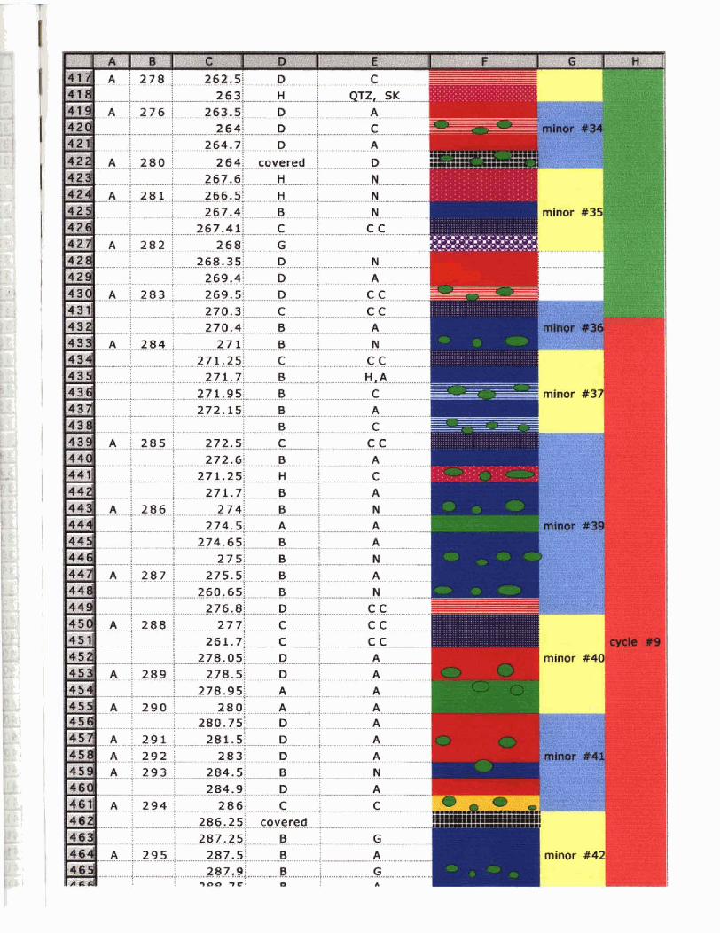
In this section, between stations A 103 and A 298 I have

extracted 8 major bundles of cycles. These bundles are based on

the changes in dominant lithology. This was almost always a

variation between dominant packstone and wackestone changing into

a mudstone dominant lithology and the back again. These changes

were repetative and fairly regular. I placed the cycle boundary

where the wackestone packstone lithology reappeared. Considering

the 3.2 Ma the frequency of these cycles is about 400,000 years.

This is fairly close to the 413,000 year cycle, but not exactly.

I think this is a result of the last cycle not being complete with

in our sample area.

Within these bundles there seems to be a smaller cyclic

pattern. This pattern is more vividly expressed in some places

than it is in others. For example in the twenty meters between

stations A 161 and A 181 There are three minor cycles. In other

areas such as between stations A 135 and A 152 there are massive

beds of cherty mudstone. This I would attribute, not to the

Tierney 8

cessation of cycling, but to the depth of water not changing

enough to make this deep water lithology shift.

I chose these cycles based on the model developed by Algeo et

al. (1992). The model predicts that there well be a thin bedded

nodular argillaceous wackestone at the base. This will be capped

by a bedded chert. Above this unit will be a massive fossil

bearing wackestone, a burrowed wackestone and finally by a cross

bedded fossil/oolitic grainstone. Most of the time in this

section the top part of the model cycle doe not appear.above the

burrowed fabric wackestone. The model predicts that this cycle

will range in thickness between 3 and 30 meters. Most of these

fall at the smaller end of that range. In total I defined 43

minor cycles. I believe that there are places where the cyclicity

of the rock is hard to see because the water at the time was a

particularly high stand and the deposition surface was below a

level of frequent lithology change.

In an attempt to define the frequency of this cycle we will

again consider our 3.2 Ma which we have defined earlier. Within

this time 43 minor cycles yield a frequency of 74,418 years. If

all the cycles could be defined I think that these cycles would

prove to be the obliquity cycle.

Conclusion

The cyclicity of these rocks is excellent. They repeat

Algeo's model cycle in a slightly abbreviated way, again and

again. The frequency of these cycles would be interesting to

study in more detail and in conjunction with the sequence

stratigraphy and a high resolution sea level curve of the time.

Tierney 9

Algeo, Thomas J., Rich Mark. 1992. Bangor Limestone; depositional environments and cyclicity on a Late Mississippian carbonate shelf. S Southeastern Geology. Vol 32, no 3. Durham, NC : Duke University, Department of Geology, Feb, 1992.

Berger, A.L., 1989. Pre-quaternary Milankovitch frequencies. Nature, 342:133.

Croll, J., 1875. Climate and Time in their Geological Relations. Appleton, New York, N. Y.

Emiliani, C., 1955. Pleistocene Temperature. J. Geol., 63: 538-578.

Groves, John R., Nemyrovska, Tamara I., Alekseev, Alexander S., 1999. Correlation of the Type Bashkirian Stage (Middle Carboniferous, South Urals) with the Morrowan and Atokan Series of the Midcontinental and Western United States. Journal of Paleontology. 73(3). pp. 529-539

Heckle, Philip H., Lambert, Lance L., Manger, Walter L., 1990. The Atokan/Desntoinesian boundary in North America; preliminary considerations for selecting a boundary horizon. CFS. Vol. 130 p. 307- 318.

Hess, Jurgen C., ~ippolt, Hans J., Burger, Kurt. 1999. High-precision

40Ar/39Ar spectrum dating on sanidine from the Donets Basin, Ukraine: evidence for correlation problems in the Upper Carboniferous. Journal of the Geological Society, London, Vol 156. pp 527-533.

Peppers, Russel A., 1996. Palynological correlation of major Pennsylvanian (Middle and Upper Carboniferous) chronostratigraphic boundaries in the Illinois and other coal basins. GSA Memoirs 188. GSA Inc. Boulder Co.

pp. 111

Schwarzacher, W., 1993. Cyclostratigraphy and the Milankovitch Theory. Elsevier, New York, N.Y. pp 225.

Scotese, Christopher R. 2002. Paleogeographic reconstruction of the Late Carboniferous, 306 Ma. www.scotese.com.

A i 142 ! 58 !ji 0 .......... ............................................ A - + ?....! : A i 143 i 6 0; 0 ................................. A + * A ; 144 : 61.5: D ............................................ A + :

6 31 D . . . . . ; A

A 146 D ......... . A - : ttttttt.tttttt..t.s~4?.~~ii ............................ A ; 147 ; 6 6; D ............... A " * : .-.---.-....-.--.-....-L-. A : 148 i 67.5 D . ,( ................................................. *. ............................... : ............................................ A A 149 1 6 9: D A A 150 i D ................. ................................ ............................................. A 1 703: j A ; ! 1 5 f ; 7 2: : ..... D .: A

H 72.8; A C G . . . . : ; - " 1 ................... 1 ..... f.,.,.: ........... A i 152 j 73.5; H .................. ....... .... ....... A C G .................................. ; 1 : .'.-.

............... ; ................. ; 73.7; covered ... 0 C ............... 1 ................. 1 ................. 7.4.:.3: - !

minor i t

- -- -. - - -- - .-. - -

minor X I

minor # 1

minor 41

i

A j_,ss.C-2&sj-0 .---: J A C I . . , . i 232.21 _.+.+ i-L-L H 1

I."..

I????,,,.

mtnar 828

minor ~ 3 4

. . . . - . -. ," . - - , " ,i- - . .

I . '