Thermomechanical Analyses ofMetal Solidification Processes

by

Winnie c. M. Leung

Submitted to the Department of Mechanical Engineeringin Partial Fulfillment of the Requirements for the Degree of

Master of Science in Mechanical Engineering

at the

MASSACHUSETTS INSTITUTE OF TECHNOLOGY

February 1995.

Copyright 1995 Winnie C. M. Leung. All rights reserved.

The author hereby grants MIT permission to reproduce and to distributepublicly paper and electronic copies of this thesis document in whole or in part.

Signature of Author ---------------------'f'"-'t-­Department of Mechanical Enginkl'ing

Certified by: -<:~~~4Z=!:::=~------------=-_=_--:-:::-::-:-~ ;32 Dr. Peter J. Raboin

Company Supervisor, Lawrence Livermore National Laboratory

Certified by: ---~'---------_7"T_'_------------o Professor Merton C. FlemingsThesis Supervisor, Department of Materials Science and Engineering

Certified by: _

Professor Carl R. PetersonDepartmental Reader, Department of Mechanical Engineering

Accepted by: ---....-...-.,...,----"""---""---'-'--------------

4HCHiVCS

Professor Ain A. SoninGraduate Thesis Committee

1995

Thermomechanical Analyses ofMetal Solidification Processes

by

Winnie C. M. Leung

Submitted to the Department of Mechanical Engineering on January 20, 1995 inpartial fulfillment of the requirements for the degree of

Master of Science in Mechanical Engineering.

Abstract

Coupled thermal and mechanical finite element analyses were used to model

the solidification of metal castings. A constitutive material model capable of predicting

the flow strength of mushy metals was developed using rate dependent plasticity. A model

addressing the reduction in heat transfer across casting-mold interfaces was created. Ther-

momechanical analyses of a simple casting experiment generated realistic predictions

which showed some discrepancies with experimental results. Analysis of a hot tear exper-

iment was successful in providing explanations to why past experiments had failed.

Company Supervisor: Dr. Peter J. Raboin

Thesis Supervisor: Dr. Merton C. FlemingsDepartment Head of Material Sciences and Engineering

Departmental Reader: Dr. Carl R. PetersonAssociate Professor of Mechanical Engineering

I would like to express my deepest gratitude to Peter Raboin, my company supervisor, forbeing a great mentor over the past three years. I thank him for the patience, insight, andmuch appreciated optimism through the seemingly endless obstacles. I appreciate hisalways taking the time out of his hectic schedule to guide me through my work.

I am also very grateful to Professor Merton Flemings for supervising this thesis project. Ithank him for all his advice and support.

I thank Professor Carl Peterson, my departmental reader, for taking the time to read andapprove this thesis.

Thank you to everyone at Lawrence Livermore: Dale Schauer for all his help and support;Brad Maker and Art Shapiro for their help in my analysis work; Larry Sanford for alwaysbeing there to help; and Barbara Kornblum for all her advice and support, Thank you alsoto everyone who have made my stay very enjoyable.

Most of all, I thank my family and friends for their advice and encouragement. In one wayor the other, they have helped me bring this thesis to completion.

Winnie C. M. Leung

Acknowledgments

A b stract ............................................................................................................................ 3A cknow ledgm ent ....................................................................................................... 5Table of C ontents ......................................................................................................... 7List of Figures .............................................................................................................. 91.0 Introduction ................................................. ...................................................... 11

1.1 B ackground ........................................... ................................................. 111.2 Project Overview .......................................................... 11

2.0 Validation of Mechanical Analysis Results ........................................ ........ 152.1 Test Problem ............................................................... ........................... 152.2 Theoretical Solution ........................................................ 162.3 Finite Element Analysis ........................................... ................ 202.4 Comparison of Results ...................................... 21

3.0 Modeling of Casting Processes ..................................... ..... ................. 253.1 Thermomechanical Approach ......................................... ............ 253.2 Thermal Model ........................................................... 26

3.2.1 Boundary Conditions ..................................... ..... .............. 273.2.2 Modeling the Specific Heat, Cp ............................. 273.2.3 Modeling the Conductivity, K ....................................... ........ 293.2.4 Modeling of Heat Transfer Mechanisms Across

Metal-Mold Interface .......................................... .............. 303.2.5 Modeling of Material Interface ....................................... ....... 32

3.3 Mechanical Model ......................................................... 343.3.1 Temperature Dependency of Density ........................................ 343.3.2 Material Strength Constitute Model ......................................... 35

4.0 Benchmarking of Finite Element Results ........................................ ......... 414.1 Cup Casting Experiment ...................................... 414.2 Finite Element Model ...................................................... 45

4.2.1 Thermal Solution ...................................................... 464.2.2 Mechanical Solution ..................................... .............. 47

4.3 R esults ............................................ ............................................... . 544.3.1 Solidification of Casting ......................................... ............ 544.3.2 Cooling Curves ....................................................... 554.3.3 Mechanical Results ........................................... ............... 62

4.4 Conclusion ............................................................................................ 655.0 Finite Element Analysis of Hot Tear Experiment ......................................... 67

5.1 Background on Hot Tears ................................................................. 675.2 Analysis of Hot Tear Experiment ........................................ .......... 68

5.2.1 Finite Element Model .................................................................. 705.2.2 Thermal Solution ......................................................................... 715.2.3 Mechanical Analyses ..................................... .... ............... 735.2.4 R esults ........................................................................................ 73

5.3 Simplified Hot Tear Casting .............................................................. 745.3.1 Finite Element Model ................................................................. 74

5.3.2 Results ............................................................. 765.4 D iscussion ........................................... ................................................... 805.5 Conclusion and Recommendations ..................................... 81

6.0 C onclusion ............................................................................................................... 83B ibliography .................................................................................................................... 85Appendix A: Properties of Pure Aluminum ........................................ ........... 87Appendix B: Properties of Aluminum Alloy 319 ...................................... ....... 91Appendix C: Properties of Carbon Steel .......................................... ............. 95Appendix D: Properties of Al 319 and Silica Sand ...................................... ...... 97

List of Fiures

Figure Title Page1 Steel and aluminum shrink fit tube assembly 152 Finite element mesh for steel and aluminum part 223 Comparison of radial stress distributions 234 Comparison of hoop stress distributions 235 Integration of Cp value into the specific heat curve 296 Initial temperature profiles of example a) without and b) with

interface slideline 337 Variation of strain rate sensitivity with strain rate and stress 388 Cross sectional diagram showing dimensions of aluminum casting

assembly 439 a) Position of thermocouples for Aluminum experiment;

b) Position of thermocouples for Aluminum 319 experiment 4410 Finite element mesh of cup casting assembly 4511 Deformation mechanism map for pure Aluminum 4912 Strain-rate-dependent flow strength model for pure Aluminum 5213 Strain-rate-dependent flow strength model for Al 319 5314 Meshes illustrating the shrinkage experienced by solidifying casting 5415 Temperature fringe plots of aluminum solidify in steel cup 5516 Temperature history plots from thermal only analysis for:

a) the casting; b) the mold 5917 Temperature history plots from thermomechanical analyses with

rate independent flow strength model for: a) the casting and b) thesteel cup 60

18 Temperature history plots from thermomechanical analyses withrate dependent flow strength model for: a) the casting and b) thesteel cup 61

19 a) Effective stress within the pure aluminum casting as solidificationprogresses; b) detailed plot of effective stress for rate dependentmodel 63

20 Effective strain rate within Al 319 casting as solidification pro-gressed 64

21 Comparison of a) the soldified casting and b) the finite elementfinal shape prediction. 65

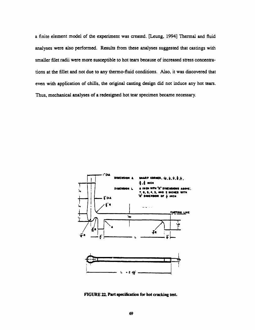
22 Part specification for hot cracking test 6923 Three-dimensional finite element mesh for redesigned casting 7024 Six nodal positions selected for temperature history data 7225 Set of cooling curves at various positions along the span of the

casting 7226 Specification for simplified hot tear casting and mold 7527 Finite element mesh for simplified hot tear casting and mold 7628 Temperature fringe plot 7729 Deformation of casting and sand mold after 300 seconds 7830 Fringes of effective stress in casting after 300 seconds shows

maximum stress in the region where bending is most severe. 79

1.0 INTRODUCTION

1.1 Background

For a casting process to be successful, the finished parts must be of sound strength

and free from defects. Designing defect free cast-metal parts by experimental trial and

error can be costly and inefficient. The motivation behind this project, undertaken by

Lawrence Livermore National Laboratory (LLNL), is to develop the means to simulate

casting processes on a computer. The ultimate goal of this project is to be able to use finite

element analyses to predict the final shape and the probable existence of any defects in the

castings. One application of interest is then to use such codes to predict the presence of hot

tears in sand castings.

To assure that the finite element analysis of a casting procedure generates realistic

predictions, the solidification process and material properties must be modeled properly.

Many current thermal and mechanical finite element computer codes depend on the user to

input the appropriate temperature-dependent parameters to model the many physical phe-

nomena which occur during solidification.

1.2 Project Overview

The objective of the work presented here was to gain an understanding of how

casting processes should be modeled for thermomechanical analysis using existing analyt-

ical tools. Because thermomechanical analyses have not been performed extensively

before, many issues still needed to be addressed. As such, this thesis project consisted of

several phases.

First, predictions from finite element mechanical analysis were compared with

theoretical calculations. Results from a finite element analysis of the stresses and strains

resulting from a simple cool down process are compared to those predicted by solid

mechanics theory in order to confirm the validity of the numerical prediction. The closed

form solution enabled assessment of the validity of the numerical predictions.

Next, a general approach to the thermal and mechanical models of a typical

finite element casting analysis is presented. A method of modeling the transfer of heat

across air gaps at metal-mold interfaces during solidification is presented. Also, a material

constitutive model capable of predicting the flow strength of metals at melting range tem-

peratures is developed.

Coupled thermomechanical analyses were then performed for a cup casting

experiment. The modeling methods developed were utilized and analytical results were

benchmarked against experimental results. By studying the discrepancies between numer-

ical and experimental results, much insight to solidification modeling was gained.

Finally, thermal and mechanical analyses were applied to a study of hot tears.

A finite element model was created for an experiment used to produce hot tear specimens.

Analyses were performed so that stress concentrations within the casting could be

observed. A simplified hot tear design was created so that the analyses can be performed

much more efficiently. Numerical analyses provided insight as to why past experiments

had been unsuccessful.

In this thesis, each of these efforts is discussed in a chapter. In addition, infor-

mation regarding the properties and parameters used in the finite element models is pro-

vided in the appendices so that the reader can repeat or modify the analyses if so desired.

2.0 VALIDATION OF MECHANICAL ANALYSIS RESULTS

Prior to using existing finite element codes to perform mechanical analyses for

complicated models, a test problem was created for which stress predictions can be

obtained from solid mechanics theory for comparison to finite element results. The closed

form solution enabled assessment of the validity of the numerical predictions.

2.1 Test Problem

The stress distribution in a shrink-fit tube during cool down was predicted by theo-

retical calculations and also by finite element analysis. The problem was modeled as a

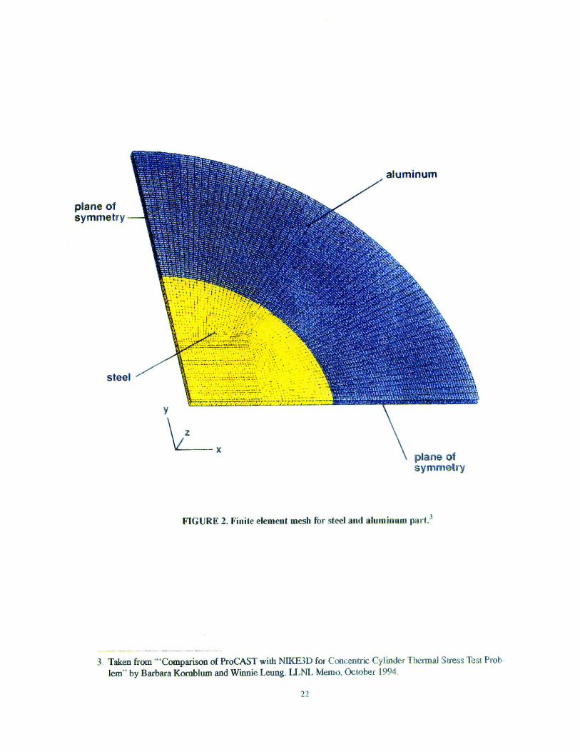
steel cylinder surrounded by an outer ring of aluminum. (See Figure 1.)

Steel

Aluminum

FIGURE 1. Steel and aluminum shrink fit tube assembly.

Aluminum SteelYoung's Modulus [psi] 10E+06 30E+06Poisson's ratio 0.33 0.29

coef. of thermal expansion [oC] 11E-06 6E-06

TABLE 1. Aluminum and steel material properties used in analyses.

15

The entire part was cooled from 300 OC to 100 (C. The part was modeled as being

constrained on the top and bottom surfaces so that there can be no axial displacements.

The aluminum and steel properties used in the analyses are shown in Table 1. Since the

coefficient of thermal expansion for aluminum is greater than that for steel, the outer alu-

minum annulus will experience more shrinkage than the inner steel core. The resulting

constraint will impose stresses on the entire part. Although this test problem is very sim-

ple, it is representative of thermal stress problems which can arise in casting processes.

2.2 Theoretical Solution

A theoretical prediction to the distribution of stresses can be obtained by starting

with the stress-strain relations expressed by Hooke's Law:

or = v(oe + Oz) + E(er -CAT) (EQ 1)

oa = v(or + Oz) + E(E~ - aAT) (EQ 2)

oz = n(or + oe) + E(Ez - aAT) (EQ 3)

where E is Young's Modulus, v is the poisson ratio, 0 is the stress, and E is the strain. The

radial, hoop, and axial components of the stresses and strains are designated by the sub-

scripts r, 0, and z respectively. Since the assembly is contrained to prohibit axial displace-

ments, we have a state of plane strain, or Ez = 0. Using this condition, Eqn. 1 can be

simplified to the form:

(EQ 4)

E (1+v)aAT+ V [] Var~ ~ I 2 1Cr -v Cy

Similarly, Eqn. 2 can be written as:

(EQ 5)

1-v vE,= (1+v)aAT+ [- -[0 -va0

[ E2 r -v 01

Expressions for the radial and hoop stresses can then be obtained by combining Eq. 4 and

Eq. 5.

(EQ 6)

E[Er -l0]r 0 1 +v

(EQ 7)

E(1-v) [[r (1 -2v) (1 +v) [ r

These two expressions are useful in rewriting the equation for radial force equilibrium:

(EQ 8)

dor or - 0- + =0dr r

as an equation in terms of the strains:

(EQ 9)

F-v rv r 1+vld+ - - a -AT1 -2vJ Ldr + dr 1-v dr

Eq. 9 can then be further simplified into a form which can be solved easily by using the

strain-displacement equations:

dur dr

uE0

(EQ 10)

(EQ 11)

Er - E 0r 0+ = 0

r

v l +v+ E - LT -+1 -v 0 1 + VI-I I - V~l

where u is the radial displacement. Recognizing also the fact that dAT/dr = 0, Eq. 9 can be

expressed as a differential equation for u(r):

(EQ 12)

du

dr2

Idu urdr 2r

which has a general solution of the form:

(EQ 13)

u= I C2

where C1 and C2 are constants of integration. Substituting this solution into the strain-dis-

placement equations, the strain in the hoop and axial directions can be expressed as:

(EQ 14)

SC C2e -= - T+ -r 2 2r

(EQ 15)

du C 1 C2dr 2 2r

These two equations can then be substituted into Eqs. 6 and 7 to obtain equations for the

radial stress and hoop stress distributions.

(EQ 16)

E C

r= [(1-2v) (1 +v)]2-

E C Ir (1-2v) (l+v) 2

SE 1C2 EaAT(l+v) r2 (1-2v)

[E EC 2 EaATL(l+v)J 2 (1-2v)

r

(EQ 17)

In order to obtain the stress distributions in the steel and aluminum, the four

unknowns C1 ,steel, C2, steel, Cl, alum, and C2, alum must be found. The value of the con-

stants can be found by considering the requirements imposed by the geometric constraint

and boundary conditions. The boundary conditions are or, steel = a0, steel in the center (r =

0); or, alum = 0 on the outer surface at r = r2; and o r, alum = or, steel at the interface at r =

r1. Also, at the interface, geometric constraint requires that Ualum = -usteel.

Upon solving the four equations generated by the constrains and substituting in

values for the material properties, the following equations can be obtained for the stress

distributions: (The unit of psi is used for the stresses and inch is used for radial position.)

* In the aluminum outer ring:

(EQ 18)3 31

o = 2.186x10 - 8.729x10 -ralum r 2

(EQ 19)

3 31G = 2.186x10 + 8.729x10 -

Oalum r2

* In the steel core:

(EQ 20)

steel = steel = -6.536x10 3

rsteeI Osteel

(Closed form solutions in terms of the material properties and geometric parameters are

not provided here because they are too complex algebraically.)

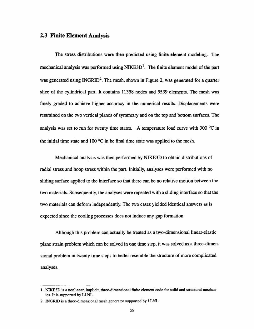
2.3 Finite Element Analysis

The stress distributions were then predicted using finite element modeling. The

mechanical analysis was performed using NIKE3D 1 . The finite element model of the part

was generated using INGRID2 . The mesh, shown in Figure 2, was generated for a quarter

slice of the cylindrical part. It contains 11358 nodes and 5539 elements. The mesh was

finely graded to achieve higher accuracy in the numerical results. Displacements were

restrained on the two vertical planes of symmetry and on the top and bottom surfaces. The

analysis was set to run for twenty time states. A temperature load curve with 300 OC in

the initial time state and 100 OC in be final time state was applied to the mesh.

Mechanical analysis was then performed by NIKE3D to obtain distributions of

radial stress and hoop stress within the part. Initially, analyses were performed with no

sliding surface applied to the interface so that there can be no relative motion between the

two materials. Subsequently, the analyses were repeated with a sliding interface so that the

two materials can deform independently. The two cases yielded identical answers as is

expected since the cooling processes does not induce any gap formation.

Although this problem can actually be treated as a two-dimensional linear-elastic

plane strain problem which can be solved in one time step, it was solved as a three-dimen-

sional problem in twenty time steps to better resemble the structure of more complicated

analyses.

1. NIKE3D is a nonlinear, implicit, three-dimensional finite element code for solid and structural mechan-ics. It is supported by LLNL.

2. INGRID is a three-dimensional mesh generator supported by LLNL.

20

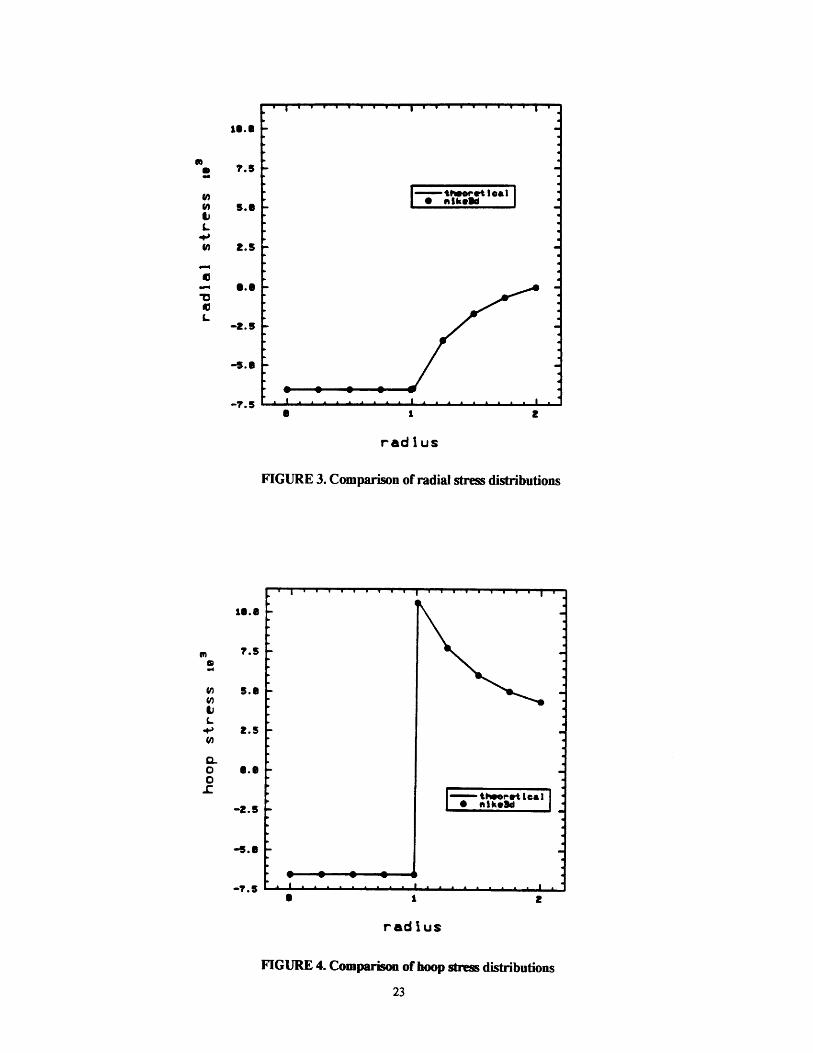
2.4 Comparison of Results

Stress predictions by NIKE3D are plotted against those predicted by Eqs. 18, 19,

and 20. The radial stress and hoop stress distributions are shown in Fig. 3 and 4, respec-

tively. It can be seen that the results are in very good agreement.

aluminum

plane ofsymmetry -

-... I,----r ~ I-..I·r ,... 7

·,t f· ·:II '~~` "C-c~·· -· i.--- · ~,.· · i··~~-··-··· .·.iL'j -·C;-r _m·

.. ,I II ·ii··, !· ; :: · -· · · .·- · .- · ·

-CLCI:--II~· 1·... I-.--.... ,,I.. ... L.('~' :'·'' ' '.

-- · ---r-.--,..·· -· ·1. . LI ···-··r t-·-· ~~"" L ~--·~I~···"~' ' ' ~· ·-

steel

zplane ofsymmetry

FIGURE 2. Finite element mesh for steel and aluminum part.

3 Taken from "'Comparison of ProCAST with NIKE3D for Concentric Cylinder Thermal Stress Test Prob

lem" by Barbara Kornblum and Winnie Leung. LLNL Memo. October 1994.

10.8

7.5

5.5

2.5

5.5

-S.8

19.0

rad us

FIGURE 3. Comparison of radial stress distributions

radius

FIGURE 4. Comparison of hoop stress distributions

----- theet I o

7

0 1

5.m

2.5

S..

-2.5

-5.8

,T W I I I I I I I I I

·I A _ .

1 1 1 I 1 1 I I

. ql

I ' ' ~ ` ~ ` - -~I I .. . . . . Ic

cc

L

3

1

3.0 MODELING OF CASTING PROCESS

For analyses of casting procedures, models which can adequately describe the

involved thermal and mechanical processes are essential to obtaining reliable results.

There are two common difficulties in performing thermomechanical analyses of solidifica-

tion processes. First, the formation of air gaps at metal-mold interfaces during solidifica-

tion needs to be modeled to obtained the correct thermal response of the system. This

effort is often complicated by the lack of understanding of the predominant modes of heat

transfer across the gap. Second, a material constitutive model capable of predicting the

liquid-solid mechanical behavior of metals needs to be developed. This problem is com-

plicated by the fact that mechanical property data at high temperatures are usually not

available, especially for metal alloys.

In this chapter, a general approach to the thermal and mechanical models used in

the finite element casting analyses is described. The attempt to address the gap formation

and material constitutive models is also discussed.

3.1 Thermomechanical Approach

The limiting capability of past technologies had dictated that thermal and mechan-

ical analyses of solidification processes be performed in an uncoupled manner. That is,

the thermal problem is solved for a fixed geometry, and then the temperature results are

used as inputs to the mechanical problem. This approach neglects the effects of the

mechanical response on the thermal problems. In problems where thermal contact is a

significant factor, the uncoupled thermal and mechanical analyses will provide only

approximate solutions. For casting processes, where the formation of air gaps at metal-

mold interface significantly diminish the transfer of heat, the coupled thermomechanical

approach is likely to provide better solutions.

Recently, LLNL has developed a coupled thermomechanical code PALM2D which

combines the thermal analysis traditionally performed by TOPAZ2D 4 and mechanical

analysis by NIKE2D. In PALM2D 5, the thermal response of an initial time step is found

and used to solve for the mechanical response. In turn, the thermal response at the subse-

quent time step is solved for the geometry determined by the mechanical analysis of the

previous time step. The mechanical response is then found for the second time step and

the process continues. This coupled approach allows for better predictions as the thermal

analysis is now performed for a deforming geometry.

The thermomechanical approach to analyzing casting processes allows for predic-

tions of phenomena which are thermally and mechanically related:

* Model the modes of heat transfer across casting-mold interfaces

* Model the mechanical behavior of metal near melting range temperatures

* Obtain predictions of temperature history and solidification time

* Predict the final shape of solidified castings and any interface gaps

3.2 Thermal Model

Many finite element analysis codes model thermal phenomena through time-

dependent or temperature-dependent values of relevant parameters supplied by the users.

4. TOPAZ2D is a heat transfer finite element analysis code supported by LLNL.

5. PALM2D is a LLNL supported finite element analysis code which uses the staggered step approach.

26

Thus, it is very important to be able to identify the significant thermal conditions and to

supply the appropriate modeling parameters.

3.2.1 Boundary Conditions

Convection and radiation boundary conditions can be applied to the exposed sur-

faces in the thermal analyses to model heat lost to the surroundings. The equation used for

the convection boundary condition is:

(EQ 21)a

q = hc[ T - Tmb ] [T- Tamb

where hc is the convective heat transfer coefficient, Tamb is the ambient temperature, and a

is the free convection exponent. For the radiation boundary conditions, the equation for

radiation heat transfer was used:

(EQ 22)

qr = E[T4 Tamb]

where E is the emittance and a is the Stefan-Boltzmann constant.

3.2.2 Modeling the Specific Heat, Cp

In the thermal analysis, the specific heat of a metal is supplied by temperature-

dependent data. Such data are usually available for common pure metals. The thermal

properties for most specific alloys, however, have not been well established. A model of

an alloy Cp data can be created by modifying that for its base metal. The specific heat val-

ues at low temperatures are usually known for most alloys. If high temperature data are

not available, then the assumption that the base metal and its alloys have similar specific

heat values at melt temperatures is made.

For analyses of metal solidification processes, the heat effects due to phase

changes must be modeled. In TOPAZ, this is achieved by modifying the specific heat data

to account for the heat of fusion, Ahf. The amount of latent heat present can be integrated

into the Cp curve since the latent heat can be defined as:

(EQ 23)

-J" C dT= Ah

where Ts is the solidus temperature and T1 is the liquidus temperature. This is also shown

graphically in Figure 5. The area of the jump in the curve is equal to Ahf. While the latent

heat is actually released at the phase change temperature, it is advisable that the width of

the spike not be made too narrow. If the width of the jump is smaller than the time step

used in the finite element analysis, the latent heat will be overlooked if the interval should

lie between two time steps.

For pure metals, the jump can take on any shape. For alloys, however, the heat of

fusion at any temperature in the freezing range corresponds to the fraction solid,fs, at that

temperature such that:

(EQ 24)

-7J C'dT

Such a model will generate a curve with several peaks at the phase transformation temper-

atures.

Cp

Tm T

FIGURE 5. Integrating Cp value into the specific heat curve.

3.2.3 Modeling the Conductivity, k

The conductivity of a metal is also supplied by temperature-dependent data. Simi-

lar to the method used to create the specific heat model, the conductivity data is taken

from literature whenever possible. The model is then completed using data for the base

metal as an estimate.

In addition, the model can be further modified to simulate the effects of natural

convection within the liquid metal in the very early stage of solidification. Convection

occurs as the hotter liquids expand and rise while the cooler liquids contract and sink.

This effect essentially sets up a circulation within the liquid, mixing the regions of differ-

ent temperature. This natural phenomenon, however, is not simulated in Lagrangian finite

element analyses. Therefore, unrealistically high thermal gradients might be predicted

within the casting. To remedy this situation, the value of the conductivity of the metal

above the melting temperature can be increased by a factor of 5 to 10 in order to decrease

the extreme temperature gradients which might be otherwise predicted. This modeling

trick is unlikely to lead to any erroneous thermal response of the system since the value of

K is increased only when the metal is still liquid.

3.2.4 Modeling of Heat Transfer Mechanisms Across Metal-Mold Interface

When a casting melt is first introduced into a cold mold, heat is transferred between

the two by means of simple liquid-solid conduction. As the casting starts to cool, a solidi-

fying shell forms and can contract away from the mold. At the same time, the mold sur-

face increases in temperature and expands. The thermal expansion and contraction lead to

the formation of interface gaps, causing the conduction through solid contacts to become

negligible. A large drop in the amount of heat transfer across the gap is observed as the

predominant mode of heat transfer changes from solid-solid conduction to convection

through the gases in the gap. To model the change in heat transfer for finite element anal-

ysis, a load curve can be used to estimate the relationship between the heat transfer coeffi-

cient across the gap and the size of the gap. Also, a gap radiation multiplier can be used to

model the effects of radiation.

As the contact between the casting and the mold diminishes, the conduction of heat

through the gases within the interface gaps becomes the predominant mechanism of heat

transfer. In modeling the correlation between heat transfer coefficient and gap size, dimen-

sional analysis can be used to find the relationship:

(EQ 25)

kho.-

where h is the heat transfer coefficient, k is the overall conductivity of the gases inside the

gap, and d is the gap width. Using this relationship, a curve can be determined for h at dif-

ferent widths as the gap formation progresses. As h is inversely proportional to d, its value

approaches infinity as the gap size approaches zero. Thus, a physical upper limit must be

applied for the value of h when no gap is present. The heat transfer can then be expressed

by:

(EQ 26)

q = hAT

where q is the heat flux and AT is the temperature difference across the gap.

It is worthwhile to note the importance of recognizing the approximate make-up of

the gases inside the gap. For instance, hydrogen is a common component in mold gases.

The thermal conductivity of hydrogen is approximately 7 times higher than that of air.

Thus, neglecting to correctly identify the gap gases can lead to a significant error in the

heat transfer coefficient model.

As the gap forms between the mold and casting, radiation heat transfer becomes

more significant. This mode of heat transfer can be described by:

(EQ 27)

qr = EE T- T1

where qr is the heat flux from radiation, E is the emittance, a is the Stefan-Boltzmann con-

stant, and T1 and T2 are the temperatures on opposite sides of the gap, such that (T1-

T2)=AT. This equation can also be expressed in the form of Eq. 10:

31

(EQ 28)

qr = hrAT = [e[T -2] [T 1 +T 2]]AT

where [eo(T2_-T22)(TI+T2)] is defined as the radiation multiplier. By comparing the val-

ues of the h in Eq. 9 and the radiation multiplier, one can determine whether the effects of

radiation are negligible.

It should be noted that the significance of radiation heat transfer varies from case

to case. Two experimental findings were cited by Campbell in his work. [Campbell,

1991] For the casting of light alloys, radiation effects are negligible as the amount of heat

transfer across the air gap by radiation is generally only of the order of 1 percent of that

due to conduction by gas. [Ho and Pehlke, 1984] However, for higher temperature metals,

such as the casting of steels in different gases or in vacuum, radiation heat transfer

becomes increasingly significant. [Jacobi, 1976]

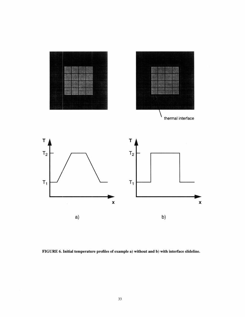
3.2.5 Modeling of Material Interface

In TOPAZ finite element thermal analysis, the application of a thermal interface

slideline allows an interface heat transfer coefficient to be defined. Furthermore, the pres-

ence of a slideline allows adjacent elements of different materials to be assigned their own

distinct initial temperatures. Without a slideline, adjacent elements of different materials

at the interface will be assigned a temperature gradient to transition the difference in tem-

perature. While a transition in adjacent temperatures can allow for easier convergence of

a thermal solution, neglecting to assign a thermal slideline can result in a significant tem-

perature profile. This point is demonstrated graphically in Figure 6.

thermal interface

T

T2

T1

x

a) b)

FIGURE 6. Initial temperature profiles of example a) without and b) with interface slideline.

T

T2

T,

X

3.3 Mechanical Model

Mechanical analyses were performed using a new solidification constitutive

model currently being developed at LLNL. We have begun studying creep behavior to

understand how metal behaves at high temperature as it experiences stresses. We have

also set up a method to model the temperature dependency of metal density.

3.3.1 Temperature Dependency of Density

The changes in density associated with the phase transformations can be modeled

by the thermal expansions and contractions using the metal's secant coefficient of thermal

expansion (CTE) at different temperatures. As phase transformations occur, a metal's

CTEs vary as it experiences thermal expansions or contractions. A set of temperature-

dependent CTE values needs to be determined. First, density data as a function of temper-

ature is needed. The density, p, can then be derived as a function of the thermal strain by

using the basic relationship of p = Mass / Volume. As the material experiences the rise in

temperature, its density decreases as it expands. Thus, the density, pT, at a higher tempera-

ture can be determined by:

(EQ 29)

T M

= [1 + 3 V0

The temperature dependency of density can then be expressed as:

(EQ 30)

In[ = 31n [ + E•I pO

where po is the density at the reference temperature. Using Eq. 30, the thermal strain, eT,

can be determined. The secant coefficient of thermal expansion, a, can then be obtained

from the relationship:

ET = a(T-Tref) (EQ 31)

Note also that eT is defined to be zero at the reference temperature, Trey; and the material is

said to be in its stress free state.

3.3.2 Material Strength Constitutive Model

The modeling of a material's constitutive properties is difficult because of scarcity

of information on the mechanical behavior of metals in the semi-solid state. While a

metal's mechanical properties at low temperature is are readily obtainable, those for ele-

vated temperatures near its melting range are usually not available. We studied how a

metal behaves near its melting point in order to model its material properties. At high

temperatures, metals show rate-dependent plasticity, or creep. Thus, the strength of liquid

metal is modeled by predicting the stress resulting from different strain rates at varying

temperatures. After determining the material strength at the extreme liquidus and solidus

ranges, a transition between the high and low temperatures can be attempted.

In steady state creep (or secondary creep), the relationship between the steady state

creep rate aP, stress a, and absolute temperature T, can be expressed as:

(EQ 32)

.peRT= Anee = Aa

where Q is the activation energy for creep, R is the Universal Gas Constant, A is the creep

constant, and n is the creep exponent. [Harper et. al., 1958] The values of the constants Q,

A, and n are unique to each material, and have to be found experimentally. At low

stresses, n has a value of about 1. At intermediate stresses, power law is observed and n

typically has a value between 3 and 8.

For common metals, data from deformation mechanism maps can be used to set up

the flow strength model. Unfortunately, such data are often not available for metal alloys.

In such cases, models are created for alloys by using data for the low temperature strength.

The mechanical behavior at melting range temperature is then modeled by using data for

its base metal. Again, a transition is created by curve fitting the data for the low and high

temperature regimes.

In the mechanical analysis code NIKE2D, a simplified and more robust form of

Eq. 31 is used. Here, the deviatoric strain rate is approximated as the plastic strain rate.

An equation of the following form is used:

(EQ 33)

o- S -

where a is the flow strength, A is the strength coefficient, S is the strength parameter, i is

the deviatoric strain rate, and m is the strain sensitivity. m can also be expressed as I/n,

where n is the strain exponent as defined in Eq. 31. S can be assigned different values to

model strain hardening effects. In our casting analysis, S has a value of 1 since no strain

hardening behavior is expected.

In setting up the flow strength model, values of m and A are found by solving Eq.

33 using any existing strength data. Temperature-dependent data points for A and m are

then inputted as load curves for the mechanical analysis. Since A and m are entered as

discrete data points at the temperatures for which data were available, the strengths at

these temperature will be given in the strength data. For temperatures in between the data

points, a linear interpolation is made for the values of A and m. The corresponding flow

strength value is then calculated. However, as indicated by Eq. 32, A is not linearly pro-

portional to a. Therefore, because of the exponential nature of the equation, there is not a

smooth transition in the curve from one point to the next. This deviation from a smooth

curve, however, can be minimized by increasing the number of data points for A and m.

Another modeling error introduced by our model is the over-estimation of flow

strength caused by the simplification of m as being dependent only on the temperature. In

reality, m is also dependent on the stress and the strain rate as indicated by Eq. 31. The

error caused by this assumption is illustrated in Figure 7. Consider, for instance, the

strength of the metal at a given temperature. In our model, the material has different

strengths depending on the strain rate. However, m is modeled to be dependent only on

temperature and does not change with the strain rate. Suppose that a value of m=ml was

determined from the creep data for a small strain rate. While the value of m actually

changes from mi to m2 as the strain rate increases, m is assigned a constant value of mI in

our model, resulting in a very large modeling error of el. This monstrous error is caused

by the large slope change as m changes from having a value of about 1 at low stresses to a

value on the order of 100 at high stresses. Similarly, if data for a large strain rate was

available, then the value of m=m 2 will be used in the strength model. The modeling error

e2 in this case is much less severe than el for the former case.

Thus, the modeling error resulting from neglecting the strain rate and stress depen-

dency of m can be minimized by determining a value of m from strength data for larger

strain rates if they are available. This will minimize the error in the flow strength predic-

tions for high strain rates at low temperatures. However, comprehensive sets of creep data

are often not available, especially for specialized metal alloys. Fortunately, this modeling

error is unlikely to have any significant effects in the analysis because the strain rates

observed at low temperatures are typically very small once the casting has solidified.

In Y

In E

FIGURE 7. Variation of strain rate sensitivity with strain rate and stress

Another limitation of the current model is that a cut-off stress level has to be

picked arbitrarily above which the value of the strength is modeled as remaining constant.

Our constitutive model is only capable of predicting the strength while the material is still

in the power law creep regime. For very high stresses, the model is no longer valid as the

material will be deforming by a different mechanism.

Finally, it should also be noted that the strength predicted by this model is only a

general approximation. In reality, the parameters of a casting procedure can greatly influ-

ence the strength of the finished parts. For instance, the finished products of sand casting

and permanent mold castings will have different mechanical properties. Other factors

such as grain size, feeding length, and cooling rate are also important.

4.0 BENCHMARKING OF FINITE ELEMENT RESULTS

In order to understand how casting procedures should be modeled for finite ele-

ment analyses, ways to benchmark results from computer models must be available.

Experimental casting results can be used as comparison with numerical results. For this

purpose, experimental castings of aluminum in a steel cup were made. The thermal and

mechanical responses of the system were observed and measured. Subsequently, the prob-

lem was modeled using finite element analysis. The finite element predictions were then

compared to experimental data.

The availability of a benchmarking tool allowed assessment of the success of the

thermal only and thermomechanical analyses. In addition, modeling approaches dis-

cussed in Chapter 3 were utilized and evaluated. The cup casting experiment was chosen

as a benchmarking tool because it was simple to conduct. Also, the experiment can be

accurately modeled using two dimensional finite element analysis. This is very important

since the simplicity of the finite element model permits the analyses to be done more effi-

ciently.

4.1 Cup Casting Experiment

The cup casting experiment was part of an on going research project at LLNL to

model the solidification of metal castings. The experiment involved simply pouring mol-

ten metal into a cylindrical steel cup. The mold was formed by welding a cylindrical piece

to a flat base piece. In a first experiment, pure Aluminum was poured at 730 OC into an

unheated cup at 27 OC. A second experiment was performed where Aluminum 319 was

41

poured at 757 OC into the mold at 25 OC. Upon solidification, the assembly was sawn

apart so that the cross section can be observed.

A cross sectional diagram of the casting assembly showing its dimensions is

shown in Figure 8. Thermocouples were placed throughout the casting to collect temper-

ature history data as the metal solidified. Linear-variable differential transformers

(LVDTs) were also used to capture any displacements as the casting cooled and con-

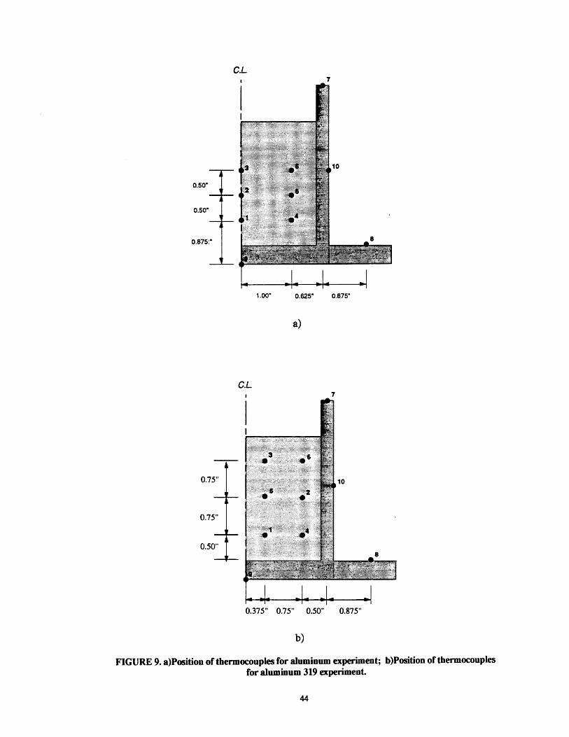
tracted. In the first experiment in which pure Aluminum was used, the thermocouples

were inserted horizontally. The position of the thermocouples is shown in Figure 9a. Dur-

ing the experiment, it was observed that the thermocouples inhibited the shrinkage of the

casting as it cooled. Therefore, in the second experiment in which Al 319 was used, the

thermocouples were inserted vertically. The new position of the thermocouples is shown

in Figure 9b.

Steel

Aluminum

N

···.............. 0. -..""" .............

'·'·'·`·'·'........................·'...........''' '''' ''' '' '

: ' ' ' ' ... ........ .........'"~"".........................:::::::::::::................... .::· · · · · · ·. .................. 5"""""".......... .......

.:....·. · ·.·..·. · ·. · ..... ... .... ·

.. .

I I ý w w I w w ý w r% %% % e% 0% % %0

% % % %% % %

J# .0 / /)/% % %% % %% %. . . . . . .

- 1.250"

3.000"

3.6

0.375"

Fiberg(4" tal

25"

lassII)

FIGURE 8. Cross sectional diagram showing dimensions of aluminum casting assembly.

Ci

! I

00- 1.500" No

C.L7

0.50'

0.50"

0.875:"

1.00" 0.625" 0.875"

a)

C.L

0.75"

0.75"

0.50"--

0.375" 0.75" 0.50" 0.875"

b)

FIGURE 9. a)Position of thermocouples for aluminum experiment; b)Position of thermocouplesfor aluminum 319 experiment.

44

I

r

r

r

4.2 Finite Element Model

A finite element model of the casting experiment was created. Since the problem

is axially symmetric, only a two dimensional cross section need be modeled. The mesh,

generated using MAZE, is shown in Figure 11. The mesh contains 1967 nodes and 1775

elements. Thermal analyses were performed using TOPAZ2D. Coupled thermomechani-

cal analyses were performed using PALM2D. The thermomechanical approach was dis-

cussed in Section 3.1.

------------------------------- 1-1-

FIGURE 10. Finite element mesh of cup casting assembly

,rr rII llI II II II

4.2.1 Thermal Solution

In our model, the melt surface and the cup's outer surfaces were cooled by convec-

tion and radiation heat loss to an ambient temperature of 25 OC. The convection boundary

condition was modeled by Eq. 21. The convective heat transfer coefficient, hC, was appro-

ximated to be 1 Btu/hr-ft2-OF (5.6786 W/m2-OK). The free convection exponent, a, was

chosen to be 0.25, which is the free convection exponent for laminar air flow over vertical

or horizontal plates. Radiation heat transfer was modeled by Eq. 22. A value of 0.7 was

used for the emittance in the equation for radiation heat transfer. In addition, an adiabatic

boundary condition was assigned to the section at the base of the cup which was supported

by a thick fiber glass block.

In the thermal only analyses, thermal conduction between the casting and the mold

is assumed since the analyses assumes a fixed geometry. A thermal slideline was

assigned at the casting-mold interface and the interface heat transfer coefficient was

approximated as 1000 W/m2-OK.

In the coupled thermomechanical analyses, the transfer of heat across interface

gaps was modeled by the approach discussed in Section 3.2.4. A load curve was set up to

model the gap heat transfer coefficient using Eq. 25. k was chosen to be 0.02414 W/m-oK,

which is the conductivity of air at room temperature. It is valid to assume that the gap

formed at the interface consisted mostly of air since our experiment involved an open

mold. In our analysis, a limiting value of h=10000 W/m2-OK was applied for a gap size of

zero. This value was chosen as an order of magnitude estimate of the heat transfer coeffi-

cient in the presence of a perfect contact interface. 6 This high value of h is likely to be

accurate only in the very early stage when the thermal contact is still excellent. In addi-

tion, radiation heat transfer across the gap was also modeled using Eq. 27. The emissivity

was estimated to be about 0.85.

Thermal properties of pure Aluminum were available in literature and are shown

in Appendix A. For Al 319, only the thermal properties at low temperatures were avail-

able. 7 The thermal data were then completed by approximating the thermal properties of

Al 319 at melt temperatures to be the same as that for pure Aluminum. The thermal prop-

erties for Al 319 used in the thermal model can be found in Appendix B. Also, for both

metals, the latent heat of fusion quantity was integrated into the specific heat curve as

described in Section 3.2.2. The conductivity values were increased by a factor of 10 in the

liquidus range to model the circulation of the cooling liquid metal due to natural convec-

tion.

4.2.2 Mechanical Solution

A mechanical interface slideline was applied between the cup and the casting so

that the two can deform independently. Nodes along the center line were constrained in

the horizontal direction to form the symmetry plane. Nodes along the bottom of the cup

were constrained in the vertical direction to model the physical support. In addition, a

downward body force was applied to model gravitational effects.

6. "Heat Transfer Data Book" by General Electric Company Corporate Research and Development.November 1970.

7. "Aluminum 319.0", Alloy Digest, May 1985.

The mechanical material properties of pure Aluminum and Al 319 can also be

found in Appendix A and B. Such data were available only for lower temperatures. Near

the liquidus ranges, the metal properties changes drastically as it becomes mushy and

retains little strength. Using thermomechanical analyses, we studied the importance of

strain rate dependence on the strength of the castings.

PALM2D analyses were first performed using a strain rate independent yield

strength model. (Shown in Table B5 in Appendix B.) The values for the yield stress were

determined by an "iterative" process. That is, initial values were chosen and the analysis

was performed. The predicted approximate strain rate within the part was observed and

the corresponding yield stress predicted by the rate dependent model was then used as the

material yield strength for future analyses. This method is not always feasible though.

The stresses predicted by the rate dependent model are typically too small to achieve con-

vergence in the rate independent solution. The low strength caused the rate independent

analyses to hourglass and deform wildly. Because of this numerical difficulty, the yield

strength had to be made arbitrarily higher so that the solution would not diverge.

Subsequently, analyses were also performed using a strain rate dependent strength

model using the approach which was described in Section 3.3.2. To construct the flow

strength model for pure Aluminum, data from a deformation mechanism map were used.

(Shown in Figure 11.) Eq. 33 was used to obtained the parameters necessary to create the

model. (Repeated here in Eq. 34 for convenience.)

TEMPERATURE. CC)

In

@I._1

HOMOLOGOUS TEMPERATURE, /TM

FIGURE 11. Deformation mechanism map for pure Aluminum.8

(EQ 34)

u= S -[Aý]A

The values of m and A are used as inputs in the mechanical finite element code to deter-

mine the rate dependent strengths. A and m are entered as discrete data points at intervals

of temperature. As discussed earlier, because of the non-linear nature of Eq. 34, increas-

ing the number of data points will increase the smoothness of the flow strength curves

generated.

The temperature-dependent values of m are determined by reading from the defor-

mation mechanism map the strengths at two different strain rates for a given temperature.

Substituting these values into Eq. 34, m can be determined by solving:

8. Taken from Frost and Ashby, 1982.

(EQ 35)In [ol/0 2]m=

In -2

and approximating for now that A1 equals A2. After obtaining values for m, A can simply

be determined by solving Eq. 34. A simple computer algorithm was then written which

used the data points for m and A to generate the strain dependent models. Figure 12

shows such a plot of the flow strength model for pure Aluminum. Example curves are

shown for the strain rates of 10-1, 10-3, 10-5 , and 10-7 per second.

The constitutive model for Al 319 was created similarly. Our efforts were compli-

cated by the fact that we only had a few data points to base the model on. (Shown in Table

2.) Unfortunately, the data were also for extremely small strain rates, (2.8x10 -1l and

2.8x10-ll per second), making the model even less accurate.

Table 2. Creep Data for Aluminum 319. 9

Values of m and A for Al 319 were then computed for the temperatures for which

the creep data were available. Since the alloy has a melting range of 789 OK to 878 oK, the

flow strength was approximated as that of pure aluminum above 650 OK. A transition

9. "Aluminum 319.0", Alloy Digest, May 1985.

Temperature Stress [psi] Stress [psi][K] creep rate: 0.0001%/hr. creep rate: 0.00001%/hr.

373 25000 24500

422 20500 17500

477 13500 10000

between the two regimes was then found by approximating a curve fit. In addition, a cut-

off in the stress level was imposed on the model beyond which our model is considered

invalid. Figure 13 shows a plot of the Al 319 rate-dependent strength model. The data

points used for m and A in the analysis are shown in Appendix B. It can be observed that

m was found to have a value of about 1 at the liquidus temperature; 0.25 near the solidus,

and only about 0.01 at room temperatures.

Ez~ 100Co

00)0.

U)_

0.2 0.3 0.4 0.5 0.6 0.7 B.9 0.9 1.0

temperature [K] 103

FIGURE 12. Strain-rate-dependent Flow Strength Model for Pure Aluminum

is(0

0crzS

- e

0.2 0.9 0.4 0.5 0.6 B.7 0.9 0.9

temperature [K] 103

FIGURE 13. Strain-rate-dependent Flow Strength Model for Al 319.

1.0

4.3 Results

4.3.1 Solidification of Casting

Meshes detailing the deformation of the cooling casting are shown in Figure

14. Temperature fringe plots of the aluminum solidifying in the steel cup are shown in Fig-

ure 15. By studying these plots, the cooling process can be better understood.

In the early stages of solidification, the outer region of the aluminum casting

begins to cool rapidly as it transfers heat to the cup. The top surface begins to drop near

the cup as the casting contracts. A well defined gap forms along the side wall. On the bot-

tom interface, small openings can be found near the axis. As solidification progresses, the

outer region of the ingot has become solid and the inner core region continues to cool. A

crater is formed on the top surface in the center as the core region cools and contracts.

Once the entire casting has solidified, there is no longer any significant changes in shape

and only small degrees of overall shrinkage are observed.

a.

'&K-

ti i i i i i ii -" i i , i I I

FIGURE 14. Meshes illustrating the shrinkage experienced by solidifying casting.

54

i

_i

m I/

-~i~ig~

o (V

) U

) co

-4 o

SO

(v

0 d

O

( N

W

G O

5 r: Ti I :i t

i t i i

0 N

to 00

0 C

O

V-

.4 1 Q

(D

(0 (0•

f€ "-

'-.-I-, (0

G

co

co •

CL

E

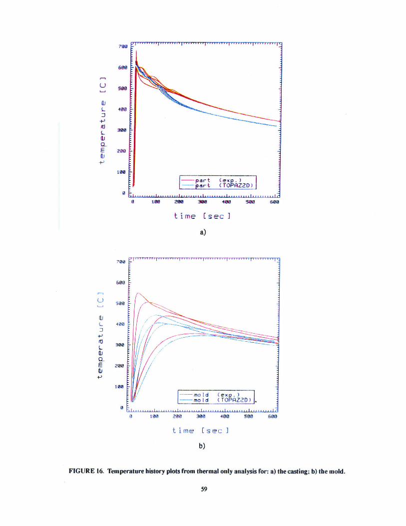
4.3.2 Cooling Curves

The temperature history plots generated by the TOPAZ2D thermal only analy-

sis of Al 319 is shown in Figure 16. The PALM2D thermomechanical analyses for Al 319

also generated cooling curves for the case with the strain rate independent flow strength

model, which is shown in Figure 17. That for the rate dependent model is shown in Figure

18. By comparing these curves with the experimental thermocouple data, insight into the

finite element models can be gained.

From these plots, it can be observed that the two thermomechanical analyses

generated cooling curves which are about identical, with the rate depend model predicting

just slightly lower cooling rates with the casting. The thermal only analysis with a con-

stant interface of h = 1000 W/m 2 -oK, however, predicted cooling curves which showed

more discrepancies with experimental results. In the early stages of solidification, the

results are still comparable. As the gap forms at the casting-mold interface, however, the

cooling rates decreases. From this point, the numerical cooling rates start to deviate from

the experimental results because the constant-h model did not address the drop in heat

transfer caused by the gap.

Furthermore, the curves in Figure 18a suggest that the value of h is higher than

1000 W/m 2-OK initially. While the molten metal is still in good contact with the mold,

much heat is rapidly transferred to the mold during the experiment, raising the mold tem-

perature to as high as 550 OC in less than 20 seconds. This behavior is not predicted in the

analyses. A comparison of the curves in Figure A clearly confirms the fact that the heat

transfer across the casting-mold interface is indeed very high in the beginning. As solidi-

fication continues, however, the transfer of heat decreases as interface gaps form. Thus, h

must take on values which change as solidification progresses in order to obtain better

thermal results.

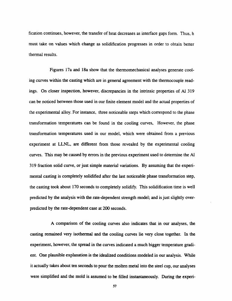
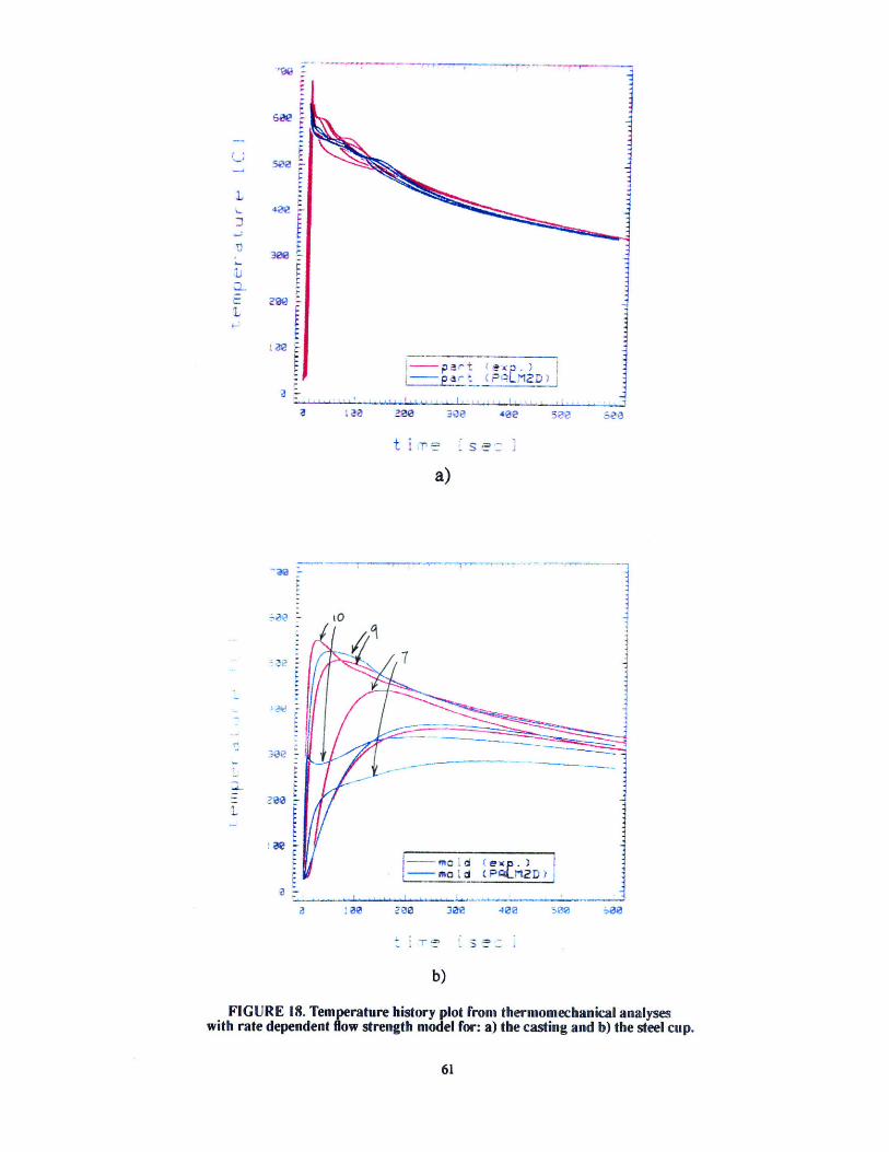
Figures 17a and 18a show that the thermomechanical analyses generate cool-

ing curves within the casting which are in general agreement with the thermocouple read-

ings. On closer inspection, however, discrepancies in the intrinsic properties of Al 319

can be noticed between those used in our finite element model and the actual properties of

the experimental alloy. For instance, three noticeable steps which correspond to the phase

transformation temperatures can be found in the cooling curves, However, the phase

transformation temperatures used in our model, which were obtained from a previous

experiment at LLNL, are different from those revealed by the experimental cooling

curves. This may be caused by errors in the previous experiment used to determine the Al

319 fraction solid curve, or just simple material variations. By assuming that the experi-

mental casting is completely solidified after the last noticeable phase transformation step,

the casting took about 170 seconds to completely solidify. This solidification time is well

predicted by the analysis with the rate-dependent strength model; and is just slightly over-

predicted by the rate-dependent case at 200 seconds.

A comparison of the cooling curves also indicates that in our analyses, the

casting remained very isothermal and the cooling curves lie very close together. In the

experiment, however, the spread in the curves indicated a much bigger temperature gradi-

ent. One plausible explanation is the idealized conditions modeled in our analysis. While

it actually takes about ten seconds to pour the molten metal into the steel cup, our analyses

were simplified and the mold is assumed to be filled instantaneously. During the experi-

57

ment, however, the melt starts to solidify as soon as it splashes into the cup. Therefore, by

the time all of the melt had been poured, a substantial temperature gradient might already

exist.

By comparing the cooling curves for the steel cup, we can understand how

well our model predicted the formation of gaps. Experimental data show that the thermo-

couple (#10) in the side of the cup rises to 550 OC before dropping as solidification contin-

ued. In our analysis, however, this sharp rise is not observed. After reaching only about

210 OC, a gap opens on the side interface and the cooling rate drops drastically. As a

result, the cooling curve predicted at the rim of the cup (#7) is extremely low. On the

other hand, the predicted cooling curve at the thermocouple (#9) on the bottom of the cup

along the axis is in much better agreement. The analysis predicted a greater amount of

heat being transferred to the bottom than the experimental results. This is consistent with

the fact that our model predicted a gap at the bottom interface which is smaller than that

observed in the experiment.

766

600

U 9NA6

L 408J

1PV 30L

E 200a)Ws

zoo

700

600

U see

L 400

300L

E 2o010

100

?00

600

U 5•0

dJ400g.i-)roL •10o

€3_E •o0

+:,

lOO

0 100 200 300 400 So9 600

time I sec ]

b)

FIGURE 16. Temperature history plots from thermal only analysis for: a) the casting; b) the mold.

- part (expZ)part (TOPAZ2D)

.! ......€ .. . . .. .! . . .. . . . .. . . . . .| . . .. . . ! .. . . . .h

-;-

/

-- mol d (exp.)-- mo Id (TOPZ2D)

.LL I ll L f1 I f LIia ±ll I Jlll 1 LLLL 11 ill Lf l I t i lllli t hIill I

I

S ee ee 2 e 30 408 se see

time Esec]

a)

Sae

520a

-~-~:

=

b)

FIGURE 17. Temperature history plot fron thermomechanical analyseswith rate independent flow strength model for: a) the casting and b) the steel cup

60

-LIL~ ----r --I.· · · ·L.r~-i·--r~-L--L( 1 '-_--~

rc------ ·----- ·----

PPRI -

a i 121 ?A-Oi 30e. 4JBJ2 50? S-2

ii ~E-

;d~~·

E~BE!

13e

~

ri

I -

~ __ __

j~3j~

ý'M :380 410e S 50 1

10 -1

b)

FIGURE 18. Temperature history plot from thermomechanical analyseswith rate dependent flow strength model for: a) the casting and b) the steel cup.

61

rt

tr

i

E

a

a

4QP

~c*-~~

r --~ t 2 D..

~)cd

• a • ( PqLM2DI:

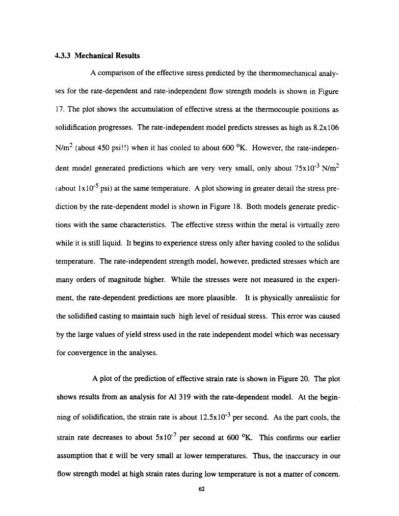
4.3.3 Mechanical Results

A comparison of the effective stress predicted by the thermomechanical analy-

ses for the rate-dependent and rate-independent flow strength models is shown in Figure

17. The plot shows the accumulation of effective stress at the thermocouple positions as

solidification progresses. The rate-independent model predicts stresses as high as 8.2x106

N/m 2 (about 450 psi!!) when it has cooled to about 600 OK. However, the rate-indepen-

dent model generated predictions which are very very small, only about 75x103l N/m 2

(about 1x10-5 psi) at the same temperature. A plot showing in greater detail the stress pre-

diction by the rate-dependent model is shown in Figure 18. Both models generate predic-

tions with the same characteristics. The effective stress within the metal is virtually zero

while it is still liquid. It begins to experience stress only after having cooled to the solidus

temperature. The rate-independent strength model, however, predicted stresses which are

many orders of magnitude higher. While the stresses were not measured in the experi-

ment, the rate-dependent predictions are more plausible. It is physically unrealistic for

the solidified casting to maintain such high level of residual stress. This error was caused

by the large values of yield stress used in the rate independent model which was necessary

for convergence in the analyses.

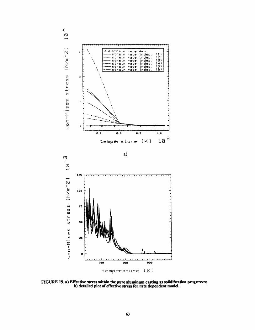
A plot of the prediction of effective strain rate is shown in Figure 20. The plot

shows results from an analysis for Al 319 with the rate-dependent model. At the begin-

ning of solidification, the strain rate is about 12.5x10-3 per second. As the part cools, the

strain rate decreases to about 5x10-7 per second at 600 OK. This confirms our earlier

assumption that e will be very small at lower temperatures. Thus, the inaccuracy in our

flow strength model at high strain rates during low temperature is not a matter of concern.

62

C0

0.7 0.8 0.9 1.8

10temperature E[K

79

70 8900 908

temperature £K I

FIGURE 19. a) Effective stress within the pure aluminum casting as solidification progresses;b) detailed plot of effective stress for rate dependent model.

-s-strain rate dep.- strain rate indep. (1)---- strain rate Indep. (2)-- strain rate indep. (3)---- strain rate Indep. (4)---- strain rate Indep. (5)--- strain rate indep. (6)

N

N`

A1 319 (rate dep. )

17.5

15.0

12.5

18.8

7.5

5.e

2.5

0.8

70ee see see

temperature [K]

FIGURE 20. Effective strain rate within Al 319 casting as solidification progressed.

A comparison of the final shape prediction generated by thermomechanical

analyses and the shape of the actual casting is shown in Figure 21. The analysis predicted

a slighter cratering on the top surface and a side gap which is larger than that observed in

the experimental casting. On the bottom interface, the analysis predicted only a very

small gap. Graphical comparisons of the gap sizes are not provided in this work because

they are not indicative of the success of the analysis. Both the experimental procedure and

the analysis are very sensitive to the process parameters, and can generate results which

are very different from trial to trial.

miS)

T--4

jI

I . ... I . . . -I..... ...... .. I

max. displacement[inches]

0.01185

0.02295

0.03402

0.04512

0.05618

.Jm71 0

L~J Jv

0.08945I ~1

)55

61

272

78UP

FIGURE 21. Comparison of a) the solidified casting and b) the finite elementfinal shape prediction.

V.IA 7

O A7 RA

4.4 Conclusion

The simplicity of the cup casting experiment allows parameter studies to be

performed efficiently. In our study, the interface gaps were confirmed to significantly

reduce the cooling rate of the assembly. Thermomechanical analyses were then performed

to address the deforming geometry. To model the strength of a metal near the melting

temperature, a constitutive material model was created in which the strain rate dependency

of a metal's flow strength was addressed. This model has been found to generate more

realistic predictions of the residual stress upon solidification than the traditional strain rate

independent model. The approach of using gap convection to model the transfer of heat

across inter face gaps was also successful in modeling the decrease in cooling rate caused

by the opening. Discrepancies in experimental and analytical results were difficult to rec-

oncile because of the great number of process parameters involved.

The benchmarking of the experimental and finite element results is difficult.

The thermocouples and LVDTs used during the experiment had introduced too many dis-

turbance to the solidification process. The thermocouples conduct heat from the melt,

thereby recording cooling rates which can be significantly higher than those in other

regions of the casting. Also, the LVDTs inhibit the casting from shrinking freely as it

cools. Thus, the experiment had introduced some uncertainty into the data.

Further finite element studies and better controlled experiments are necessary

to perfect the casting model. It is unknown at this time why the finite element model did

not predict the deformations upon solidification more precisely. For future studies, fine

tuning the high temperature material properties and improving the imposed thermal condi-

tions are recommended.

5.0 FINITE ELEMENT ANALYSIS OF HOT TEAREXPERIMENT

After gaining experience in modeling casting problems, analyses for hot tear

studies were performed. Previously, finite element analyses were performed for an exper-

iment designed for benchmarking the hot tear susceptibilities of different alloys. Thermal

and fluid analyses have been completed for a hot tearing test of aluminum sand castings.

Mechanical analyses were deemed necessary before any predictions of hot tears can be

made.

Attempts to perform loosely coupled thermal and mechanical analyses for the

hot tear experiment were unsuccessful. The mesh for the model was very large and ineffi-

cient to debug. Finally, a much simpler casting assembly with the same characteristics as

the hot tear experiment was designed so that results can be obtained more efficiently.

5.1 Background on Hot Tears

In sand casting processes of metal alloys, the presence of hot tears is one of

many common causes of defects. Hot tearing can occur as a metal part solidifies in the

sand mold. A casting develops tears if the stresses it experiences due to solidification and

cool down shrinkage are greater than the ability of the metal to withstand them. The cause

of hot tears is a complex matter. Factors such as solidification conditions, material proper-

ties, and part geometry all affect a casting's hot tear susceptibility. Typically, alloys are

more prone to hot tears than pure metals because alloys solidify over a range of tempera-

tures rather than at a discrete temperature. Hot tears take place in an alloy casting while it

is still in the mushy zone, where both liquid and solid states coexist.

Hot tears result from stress concentrations within a casting caused by factors

such as hindered contractions, hot spots, or extreme temperature gradients. The geometri-

cal configuration of a casting can also have significant effects on its hot tearing tendency.

Inadequate fillets in sharp corners can set up high stresses during solidification. Abrupt

variations in the casting's thickness cause large variations in cooling rate, resulting in hot

spots. In addition, sections which are I-shaped or U-shaped also experience high stresses

during cooling due to restriction from the mold. In addition to the factors mentioned

above, there are still many other issues which influence hot tearing susceptibility. Metal-

lurgical casting parameters such as g din size, alloy composition, molding sand compress-

ibility, and gas content of the melt all have significant effects.

Engineers and scientists at General Motors Research Laboratories, Oak Ridge

National Laboratory, Sandia National Laboratories, and LLNL have undertaken a study on

hot tears in order to develop an aluminum alloy with high resistance to hot tearing. The

project entailed designing and executing an experiment to be used for benchmarking of

existing and any newly developed alloys. LLNL's role in the project was to provide the

metallurgists and material scientists with insights to the casting procedure gained by per-

forming finite element analyses of the experiment.

5.2 Analysis of Hot Tear Experiment

The experiment used was modeled after that developed by E.J. Gamber. [Gam-

ber, 1959] Designed to show that cracks are more probable at sharp internal angles, the

experiment entailed casting parts of various fillet radii. The specification for the speci-

mens is shown in Figure 22. The effects of using end chills were also studied. Previously,

68

a finite element model of the experiment was created. [Leung, 1994] Thermal and fluid

analyses were also performed. Results from these analyses suggested that castings with

smaller filet radii were more susceptible to hot tears because of increased stress concentra-

tions at the fillet and not due to any thermo-fluid conditions. Also, it was discovered that

even with application of chills, the original casting design did not induce any hot tears.

Thus, mechanical analyses of a redesigned hot tear specimen became necessary.

uaa, asna,. *r..*.+.*.

a IoNc Wff" VA' DIalmOes AGovI;.6, S,4, . aNm a lme$es wrN

A'" *miNa O•e or ICmen

04ajIfe LuNe1-_

L

.I,.r.FL

I s

L

FIGURE 22. Part specification for hot cracking test.

42I

.. P-.

!

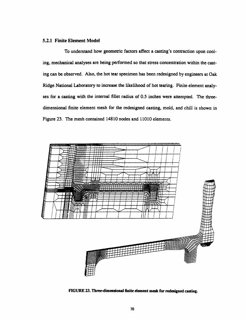
5.2.1 Finite Element Model

To understand how geometric factors affect a casting's contraction upon cool-

ing, mechanical analyses are being performed so that stress concentration within the cast-

ing can be observed. Also, the hot tear specimen has been redesigned by engineers at Oak

Ridge National Laboratory to increase the likelihood of hot tearing. Finite element analy-

ses for a casting with the internal fillet radius of 0.5 inches were attempted. The three-

dimensional finite element mesh for the redesigned casting, mold, and chill is shown in

Figure 23. The mesh contained 14810 nodes and 11010 elements.

FIGURE 23. Three-dimensional finite element mesh for redesigned casting.

After creating the finite element mesh, thermal and mechanical analyses can be

performed. A loosely coupled thermomechanical approach is taken because the features

of PALM2D have not yet been implemented for three dimensional analyses. In a loosely

coupled thermomechanical approach, thermal analysis is first performed. The temperature

results are then used as inputs to a mechanical analysis.

5.2.2 Thermal Solution

Thermal only analyses were performed for a system which has already been

filled. The Aluminum 319 was initially at 715 OC. The sand mold and copper end chill

were initially at 25 OC. Analyses were performed in ProCAST lo with the heat transfer

coefficient at the casting-chill interface estimated as 2000 W/m 2 oK. The heat transfer

coefficient at the chill-sand interface was estimated to be 200 w/m 2 OK. Fluid analyses

were not performed since it was confirmed in the previous study that fluid effects during

the filling process do not affect the accuracy of the thermal results.

The temperature versus time data were predicted at five different positions in

the casting. There are four points distributed along a center line in the body, and one point

in the center of the variable radius. Figure 23 shows the six nodal positions. The cooling

curves generated from the ProCAST analyses are shown in Figure 24.

10.ProCAST is a finite element analysis package for casting systems. ProCAST is a trademark of UES, Inc.,Dayton, Ohio.

FIGURE 24. Six nodal positions selected for temperature history data.

a 1 a a

time (seconds] i3'U

FIGURE 25. Set of cooling curves at various positions along the span of the casting.

1.1

8.9

e..

8.7

U.6

on'4

L

0

L41f,.CLi.4414A

5.2.3 Mechanical Analyses

Mechanical analyses are performed using NIKE3D. The temperature results

from ProCAST were processed by ProCONVERT 11 into a form compatible as tempera-

ture time-state data for NIKE3D. A simple elastic-plastic material model is used (Shown

in Appendix D.) The properties for silica sand were estimated from results of triaxial

compression tests for dense fine silica sand. [Duncan et. al., 1970] In addition, a mechan-

ical slideline is applied at all of the material interfaces to allow the casting to deform inde-

pendently of the casting and mold.

5.2.4 Results

Unfortunately, the mesh for the hot tear experiment is too large, making the

finite element analyses very costly and time ineffective. Many difficulties were encoun-

tered in achieving convergence of solution in the initial time steps. This was due to the

lack of experience in performing such analyses and the inefficiencies of a large mesh.

Debugging was almost impossible since the model required a typical turn-around time of

about 24 hours on the Cray Computers as the series of iterations and reformations are per-

formed to attempt convergence.

As a result, analyses of the hot tear experiment were suspended. Instead, a

much simpler model was created which has all the characteristics of the hot tear experi-

ment. This smaller mesh allowed us to gain insight to the hot tear experiment in a much

more effective manner.

I1.ProCONVERT is a program used at LLNL to make ProCAST temperature ouputs compatible asNIKE3D input.

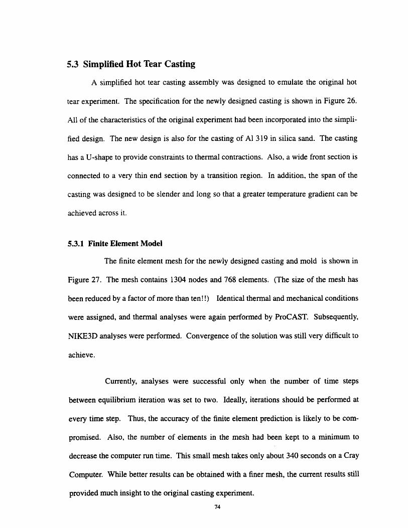
5.3 Simplified Hot Tear Casting

A simplified hot tear casting assembly was designed to emulate the original hot

tear experiment. The specification for the newly designed casting is shown in Figure 26.

All of the characteristics of the original experiment had been incorporated into the simpli-

fied design. The new design is also for the casting of Al 319 in silica sand. The casting

has a U-shape to provide constraints to thermal contractions. Also, a wide front section is

connected to a very thin end section by a transition region. In addition, the span of the

casting was designed to be slender and long so that a greater temperature gradient can be

achieved across it.

5.3.1 Finite Element Model

The finite element mesh for the newly designed casting and mold is shown in

Figure 27. The mesh contains 1304 nodes and 768 elements. (The size of the mesh has

been reduced by a factor of more than ten!!) Identical thermal and mechanical conditions

were assigned, and thermal analyses were again performed by ProCAST. Subsequently,

NIKE3D analyses were performed. Convergence of the solution was still very difficult to

achieve.

Currently, analyses were successful only when the number of time steps

between equilibrium iteration was set to two. Ideally, iterations should be performed at

every time step. Thus, the accuracy of the finite element prediction is likely to be com-

promised. Also, the number of elements in the mesh had been kept to a minimum to

decrease the computer run time. This small mesh takes only about 340 seconds on a Cray

Computer. While better results can be obtained with a finer mesh, the current results still

provided much insight to the original casting experiment.

74

sc

cIvriucu

oIn

if-

i- o

m

Ir

6lin/

mm

ý

i i

TC)tn

• I

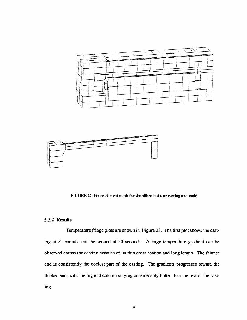
FIGURE 27. Finite element mesh for simplified hot tear casting and mold.

5.3.2 Results

Temperature fringe plots are shown in Figure 28. The first plot shows the cast-

ing at 8 seconds and the second at 50 seconds. A large temperature gradient can be

observed across the casting because of its thin cross section and long length. The thinner

end is consistently the coolest part of the casting. The gradients progresses toward the

thicker end, with the big end column staying considerably hotter than the rest of the cast-

ing.

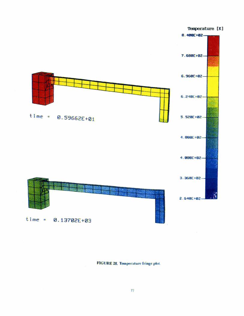
Temperature [K]S. 4@WE+82-

7.688E+82-

6. 96@E+02

6 248E+B2-

5 52•E 982--

4 .8OW8 e +82-

4. 8÷BE+8Z-

3. 368E -82 -

2. S48E .82-

FIGURE 28. Temperature fringe pkl)

2ý6 E,

,!

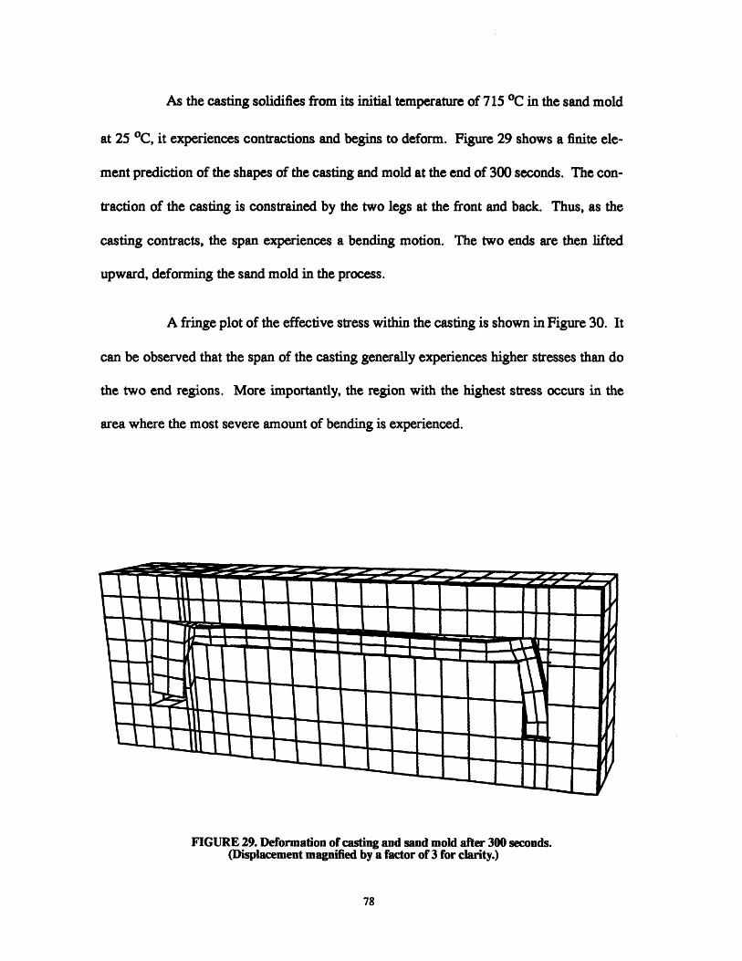
As the casting solidifies from its initial temperature of 715 oC in the sand mold

at 25 oC, it experiences contractions and begins to deform. Figure 29 shows a finite ele-

ment prediction of the shapes of the casting and mold at the end of 300 seconds. The con-

traction of the casting is constrained by the two legs at the front and back. Thus, as the

casting contracts, the span experiences a bending motion. The two ends are then lifted

upward, deforming the sand mold in the process.

A fringe plot of the effective stress within the casting is shown in Figure 30. It

can be observed that the span of the casting generally experiences higher stresses than do

the two end regions. More importantly, the region with the highest stress occurs in the

area where the most severe amount of bending is experienced.

FIGURE 29. Deformation of casting and sand mold after 300 seconds.(Displacement magnified by a factor of 3 for clarity.)

time = 0. 30000E+03fringes of eff. stress (v-m)

4. 484E+85-

3. 762E+85-

3. 119E+05-

2.477E+95-

1. 834E+85-

1. 191E+95-

5. 498E+94-

-9.433E+893-

FIGURE 30. Fringe plot of effective stress in casting after 300 seconds showsmaximumr stress in the region where bending is most severe.

.... .. I" ̧

5.4 Discussion

Although the analysis of the simplified casting design yielded only approxi-

mate predictions, it provided much insight into why the original hot tear experiment was

unsuccessful. Previously, the hot tear specimen was thought to have failed because of the

lack of temperature gradients in the span. Thus, the front leg was widened so that the

cooling rate can be decreased. This design change was made with the intention that the

metal in the widened leg will remain mushy longer and become subjected to contraction

forces as the thinner span and back leg contracted. However, for this design to induce hot

tears at the variable radius, the span must be long and slender enough so that a very sig-

nificant temperature gradient is present across the casting. The redesigned casting, how-

ever, did not have a span slender enough and was likely to be unsuccessful again in

producing hot tears in the specimens. In fact, the only effects of the widened front leg is

that the stress it experiences will be reduced because of the increase in cross sectional

area. Therefore, the region near the variable radius has actually been made less sensitive

to hot tears.

In order for hot tears to occur in a specimen, the part must have regions of

abrupt variation in cross section and extreme temperature gradients. In addition, the

geometry of the casting and mold must provide enough geometric constraint that any ther-

mal contractions in the part is hindered. Results from the finite element analyses have

shown that this condition is met neither in the original nor the simplified hot tear design.

Because the two end legs, especially the thinner back leg, are not massive enough, they do

not sufficiently prohibit the contraction of the span. As a result, the span is allowed to

contract by bending and lifting the two ends. Thus, the ends must be made massive

enough so that this bending action is minimized to provide maximum hindrance to the

contraction of the span.

5.5 Conclusion and Recommendations

Finite element analysis of the original hot tear experiment was unsuccessful

because of its large mesh size. Because of the lack of experience in performing thermo-

mechanical analyses, much debugging was required. The debugging process was very

time consuming and inefficient because the model was so cpu intensive. Therefore, a sim-

plified hot tear model with the characteristics of the original one was created. The thermal

and mechanical analyses provided insight to the flaws in the design of the hot tear speci-

men. The geometry of the part did not induce a large enough temperature gradient across

the casting. In addition, the shape of the casting provided insufficient hindrance to ther-

mal contraction in the span.

In designing a new hot tear specimen, simplicity in the geometry is important

if finite element analysis predictions are desired. As new features are being implemented

into the thermomechanical approach, much debugging and parametric studies are neces-

sary. Large models will be too time and cost inefficient for this purpose.

6.0 Conclusion

While the ultimate goal of this project was to perform thermomechanical anal-

yses for a hot tear experiment, development of the finite element model required bench-

marking analyses to be first performed for a much simpler casting procedure. Insight into

the solidification process was then applied to the hot tear analyses.

Finite element analyses of casting processes performed using the coupled ther-

mal and mechanical approach are capable of taking into consideration the changes in

geometry often present during solidification. An approach to model the transfer of heat

across interface gaps was presented. The interface gaps and surface deformations predic-

tion showed some disagreement with experimental results. The discrepancies can be

attributed to simplifications made in the finite element model which were necessary to

keep the model robust. Difficulties in controlling the experiment also introduced uncer-

tainty into the experimental data. More importantly, the solidification process is highly

sensitive; and repeated casting trials often do not generate identical results even under the

same apparent conditions. Thus, it can be concluded that our model is satisfactory in pro-

viding an approximation to the gaps and surface deformations formed during solidifica-

tion.

An approach to model the flow strength of metals at melting range tempera-

tures was also developed using rate dependent plasticity. This model was found to gener-

ate more realistic results than previous analyses using a creep rate independent model,

which had erroneously predicted high residual stresses within the casting even after com-

plete solidification.

Finite element analyses of the hot tear experiment were found to be inefficient

because of the large mesh size. A simplified hot tear design with the characteristics of the

original one was created so that analyses could be performed more efficiently. Prelimi-

nary thermal and mechanical analyses predicted flaws in the hot tear design. The geom-

etry of the casting was found to provide insufficient hindrance to thermal contraction in

the span.

Because of time limitations, analyses using the models for interface gaps and

rate-dependent plasticity flow strength were not performed. For future studies, it is rec-

ommended that the hot tear design be revised before any further analyses is performed.

While more detailed finite element meshes can generate more accurate predictions, sim-

pler models are better suited for the purposes of debugging and parameter studies. With

more experience in performing thermomechanical analyses, the interface gap and rate

dependent flow strength models can be further improved.

Bibliographv

1. "Heat Transfer Data Book", General Electric Company Corporate Research andDevelopment, November 1970.

2. Campbell, John. Castings, Butterworth-Heinemann Ltd., Oxford. (1991)

4. Crandall, S., Dahl, N., and Lardner, T. An Introduction to the Mechanics of Solids.McGraw-Hill Book Company: New York, 1978.

5. Duncan, James M., and Chang, Chin-Yung, "Nonlinear Analysis of Stress and Strainin Soils", Journal of the Soil Mechanics and Foundation Division, Proceedings of theAmerican Society of Civil Engineers, September 1970.

6. Frost, Harold J. and Ashby, Michael F., Deformation-Mechanism Maps: The Plastic-ity and Creep of Metals and Ceramics. Pergamon Press: Oxford, 1982, pp 26-27.

7. Gamber, E.J., "Hot Cracking Test for Light Metal Casting Alloys", TransactionsAmerican Founrymen Society, vol. 67, 1959. pp 237-241.

8. Harper, J. G., Shepard, L.A. and Dorn, J.E., "Creep of Aluminum Under ExtremelySmall Stresses", Acta Metallurgica, vol. 6, July 1958, pp 509-518.

9. Ho, K., and Pehlke, R. D., "Mechanisms of Heat Transfer at a Metal-Mold Interface",American Foundrymen Transactions, 1984, pp 587-598.

10. Jacobi, H. Arch. Eisenhuttenwesen, vol. 47, pp 441-446. (1976)

11. Kornblum. B., and Leung, W., "Comparison of ProCAST with NIKE3D for Concen-tric Cylinder Thermal Stress Test Problem", Lawrence Livermore national Laboratory,October 1994.

12. Leung, W., "Finite Element Analyses of Hot Tearing Test for Aluminum Sand Cast-ings", S.B. Thesis for M.I.T., May 1994.

13. McClintock, Frank A. and Argon, Ali S., Mechanical Behavior of Materials. Red-ding, Massachusetts: Addisson-Wesley Publishing Company, 1966.

14. Raboin, Peter J., "A solidification Constitutive Model for NIKE2D and NIKE3D",Lawrence Livermore National Laboratory, January 1994.

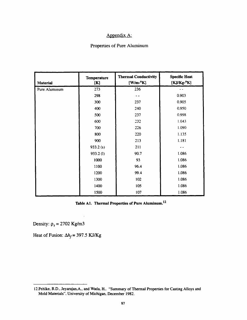
Appendix A:

Properties of Pure Aluminum

Table Al. Thermal Properties of Pure Aluminum. 12

Density: p, = 2702 Kg/m3

Heat of Fusion: Ahf= 397.5 KJ/Kg

12.Pehlke, R.D., Jeyarajan,A., and Wada, H.. "Summary of Thermal Properties for Casting Alloys andMold Materials", University of Michigan, December 1982.

a. CTE stands for Coefficient of Thermal Expansion

Table A2: Mechanical Properties of Pure Aluminum.

Temperature Flow Strength[K] [Nim2 ]

298 90.00E+06

598 45.00E+06

900 1.00E+04

933 1.00E+04

1500 1.00E+04

Table A3: Rate Independent Flow Strength for Pure Aluminum.

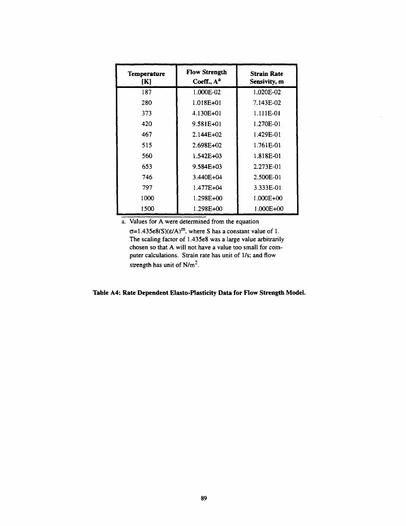
Temperature Flow Strength Strain Rate[K] Coeff., Aa Sensivity, m

187 1.000E-02 1.020E-02

280 1.018E+01 7.143E-02

373 4.130E+01 1.111E-01

420 9.581E+01 1.270E-01

467 2.144E+02 1.429E-01

515 2.698E+02 1.761E-01

560 1.542E+03 1.818E-01

653 9.584E+03 2.273E-01

746 3.440E+04 2.500E-01

797 1.477E+04 3.333E-01

1000 1.298E+00 1.000E+00

1500 1.298E+00 1.000E+00

a. Values for A were determined from the equation

o=1.435e8(S)(E/A)m, where S has a constant value of 1.The scaling factor of 1.435e8 was a large value arbitrarilychosen so that A will not have a value too small for com-puter calculations. Strain rate has unit of I/s; and flow

strength has unit of N/m2 .

Table A4: Rate Dependent Elasto-Plasticity Data for Flow Strength Model.

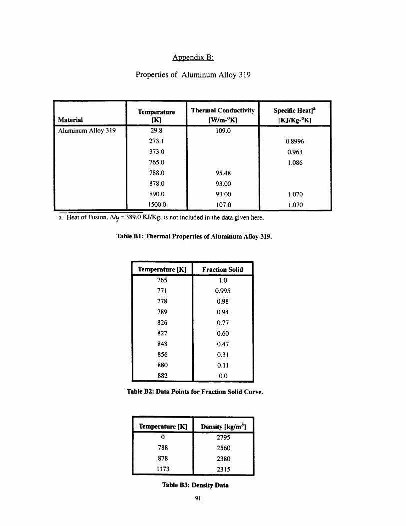
Appendix B:

Properties of Aluminum Alloy 319

Temperature Thermal Conductivity Specific Heat]a

Material [K] [W/m-OK] [KJ/Kg-oK]

Aluminum Alloy 319 29.8 109.0

273.1 0.8996

373.0 0.963

765.0 1.086

788.0 95.48

878.0 93.00

890.0 93.00 1.070

1500.0 107.0 1.070

a. Heat of Fusion. Ahf = 389.0 KJ/Kg, is not included in the data given here.

Table BI: Thermal Properties of Aluminum Alloy 319.

Temperature [K] Fraction Solid

765 1.0

771 0.995

778 0.98

789 0.94

826 0.77

827 0.60

848 0.47

856 0.31

880 0.11

882 0.0

Table B2: Data Points for Fraction Solid Curve.

Temperature [K] Density [kg/m 3 ]

0 2795

788 2560

878 2380

1173 2315

Table B3: Density Data

Temperature Young's Modulus Poisson's Ratio Secant CTEa[K] [N/m 2] [i/K]

298 69.00E+09 0.33 23.90E-06

598 69.00E+09 0.33 23.90E-06

730 50.00E+09 0.33

760 10.00E+09 0.33

788 57.69E-06

877 1.00E+09 0.33 90.97E-06

1173 72.02E-06

1500 1.00E+09 0.33

a. CTE stands for Coefficient of Thermal Expansion

Table B4: Mechanical Properties of Aluminum Alloy 319.

Temperature Flow Strength[K] [N/m 2 ]298 90.00E+06

598 45.00E+06

730 1.00E+04

790 1.00E+04

877 1.00E+04

1500 1.00E+04

Table B5: Rate Independent Flow Strength for Al 319.

Temperature[K]373

422

477

500

525

540

565

595

620

630

638

653

700

746

797

1000

1500

Flow Strengtn

Coeff., Aa

2.778E-08

4.986E-07

3.139E-06

1.317E-05

2.148E-04

4.026E-04

3.968E-03

2.147E-01

3.489E+00

1.167E+01

1.013E+01

3.566E+01

1.420E+03

7.609E+04

2.679E+04

1.582E+00

1.582E+00

a. Values for A were determined from the equation

0=1.75e8(S)(E/A)m, where S has a constant value of 1.The scaling factor of 1.75e8 was a large value arbitrarilychosen so that A will not have a value too small for com-puter calculations. Strain rate has unit of 1/s; and flow

strength has unit of N/m2 .

Table B6: Rate Dependent Elasto-Plasticity Data for Flow Strength Model.

Strain RateSensivity, m

8.774E-03

6.893E-02

1.303E-01

1.487E-01

1.594E-01

1.701E-01

1.786E-01

1.915E-01

2.000E-01

2.083E-01

2. 165E-01

2.273E-01

2.400E-01

2.500E-01

3.333E-01

1.000E+00

1.000E+00Wý

Appendix C:

Properties of Carbon Steel

Table C1: Thermal Properties of Carbon Steel

Young'stemperature Modulus Poisson's Secant CTE Yield Stress

[K] iN/m2] Ratio [1/K] [N/m2]

200 2.00E+I 1 0.3 10.0E-06 7.0E+08

1500 2.00E+ 11 0.3 10.0E-06 7.0E+08

Table C2: Mechanical Properties of Carbon Steel

(Density = 7800 Kg/m 3)

temperature Specific Heat Thermal Conduc-[K] [J/Kg oK] tivity [W/m 2 oK]

200 434 60.5

400 487 56.7

600 559 48.0

800 685 39.2

1000 1169 30.0

1500 1169 30.0

Appendix D:

Properties of Silica Sand and Al 319 used in Hot Tear Analysis

Temperature Young's Modulus Poisson's Yield Strength[K] [N/m 2 ] Ratio Secant CTE [N/m 2]298 10.000E+06 0.33 2.390E-05 9.000E+07

598 7.100E+06 0.33 2.390E-05 4.500E+07

790 1.400E+06 0.33 5.770E-05 1.000E+05

877 1.400E+06 0.33 9.100E-05 5.000E+04

1500 1.400E+06 0.33 7.200E-05 5.000E+04

Table Dl: Mechanical Properties of Aluminum 319.

Temperature Young's Modulus Poisson's Yield Strength[K] [N/m 2] Ratio Secant CTE [N/m 2]

298 6.300E+04 0.20 5.000E-06 1.000E+05

598 6.300E+04 0.20 5.000E-06 1.000E+05

790 6.300E+04 0.20 5.500E-06 1.000E+05

877 6.300E+04 0.20 6.000E-06 1.000E+05

1500 6.300E+04 0.20 6.000E-06 1.000E+05

Table D2: Mechanical Properties of Silica Sand.