The Spitzer Survey of Interstellar Clouds in the Gould Belt. VI.The Auriga-California Molecular Cloud observed with IRAC and

MIPS

Hannah Broekhoven-Fiene1, Brenda C. Matthews2,1, Paul M. Harvey3, Robert A.Gutermuth4, Tracy L. Huard5,6, Nicholas F. H. Tothill7, David Nutter8, Tyler L. Bourke9,

James DiFrancesco2, Jes K. Jørgensen10,11, Lori E. Allen12, Nicholas L. Chapman13,Michael M. Dunham14, Bruno Merın15, Jennifer F. Miller5,9, Susan Terebey16, Dawn E.

Peterson17, Karl R. Stapelfeldt18

ABSTRACT

We present observations of the Auriga-California Molecular Cloud (AMC) at 3.6, 4.5, 5.8, 8.0,24, 70 and 160 μm observed with the IRAC and MIPS detectors as part of the Spitzer Gould BeltLegacy Survey. The total mapped areas are 2.5 deg2 with IRAC and 10.47 deg2 with MIPS. Thisgiant molecular cloud is one of two in the nearby Gould Belt of star-forming regions, the otherbeing the Orion A Molecular Cloud (OMC). We compare source counts, colors and magnitudesin our observed region to a subset of the SWIRE data that was processed through our pipeline.Using color-magnitude and color-color diagrams, we find evidence for a substantial population of166 young stellar objects (YSOs) in the cloud, many of which were previously unknown. Mostof this population is concentrated around the LkHα 101 cluster and the filament extending fromit. We present a quantitative description of the degree of clustering and discuss the fraction ofYSOs in the region with disks relative to an estimate of the diskless YSO population. Althoughthe AMC is similar in mass, size and distance to the OMC, it is forming about 15 – 20 timesfewer stars.

Subject headings: infrared: general — ISM: clouds — stars: formation

1Department of Physics and Astronomy, University ofVictoria, Victoria, BC, V8W 3P6, Canada

2National Research Council Herzberg Astronomy & As-trophysics, Victoria, BC, V9E 2E7, Canada

3Astronomy Department, University of Texas at Austin,1 University Station C1400, Austin, TX 78712-0259, USA

4Department of Astronomy, University of Mas-sachusetts, Amherst, MA, USA

5Department of Astronomy, University of Maryland,College Park, MD 20742, USA

6Columbia Astrophysics Laboratory, Columbia Univer-sity, New York, NY 10027, USA

7School of Computing, Engineering & Mathematics,University of Western Sydney, Locked Bag 1797, Penrith,NSW 2751, Australia

8School of Physics and Astronomy, Cardiff University,Queen’s Buildings, The Parade, Cardiff CF24 3AA, UK

9Harvard-Smithsonian Center for Astrophysics, 60 Gar-den Street, Cambridge, MA 02138, USA

10Niels Bohr Institute, University of Copenhagen, Ju-liane Maries Vej 30, DK-DK-2100 Copenhagen Ø., Den-mark

11Centre for Star and Planet Formation, Natural His-tory Museum of Denmark, Øster Voldgade 5-7, DK-1350Copenhagen K., Denmark

12National Optical Astronomy Observatories, Tucson,AZ, USA

13Center for Interdisciplinary Exploration and Researchin Astrophysics (CIERA) & Department of Physics & As-tronomy, Northwestern University, 2145 Sheridan Road,Evanston, IL 60208

14Department of Astronomy, Yale University, P.O. Box208101, New Haven, CT 06520, USA

15Herschel Science Centre, ESAC-ESA, P.O. Box 78,28691 Villanueva de la Canada, Madrid, Spain

16Department of Physics and Astronomy PS315, 5151State University Drive, California State University at LosAngeles, Los Angeles, CA 90032, USA

17Space Science Institute, 4750 Walnut Street, Suite 205,

1

arX

iv:1

402.

6329

v1 [

astro

-ph.

GA

] 25

Feb

201

4

1. Introduction

The cycle 4 Spitzer Space Telescope Legacyproject “The Gould Belt: Star Formation in theSolar Neighborhood” (PID: 30574; PI: L.E. Allen)completed the Spitzer survey of the large, nearbystar-forming regions begun by the c2d LegacyProject (Evans et al. 2003, 2009). The cloud withthe least prior study included in the survey is thecloud we have designated as “Auriga” which lieson the Perseus-Auriga border. This cloud has alsobeen designated the California Molecular Cloudby Lada et al. (2009) since it extends from theCalifornia Nebula in the west to the LkHα 101 re-gion and associated NGC 1529 cloud in the east.We adopt the name Auriga-California MolecularCloud (AMC) to encompass both nomenclatures.

Despite the AMC’s proximity to two of themost well-examined star-forming clouds, Taurus-Auriga and Perseus, it is a relatively unstudiedregion. Several dark nebulae were noted along itslength by Lynds (1962), and CO associated withmany Lynds objects was measured by Ungerechts& Thaddeus (1987), who note the presence of a CO“cloud extending from the California nebula (NGC1499) in Perseus along NGC 1579 and LkHα 101well into Auriga” (their cloud 12). Only very re-cently has a giant molecular cloud been unam-biguously associated with the series of Lynds neb-ulae through high resolution extinction maps byLada et al. (2009) who placed its distance firmlywithin the Gould Belt (GB) at 450 ± 23 pc. Atthis distance, the cloud’s extent of 80 pc and massof ∼ 105 M� rivals that of the Orion MolecularCloud (L1641) for the most massive in the GouldBelt. For the remainder of this paper, we adoptthis distance of 450 pc for the entire AMC. This isconsistent with the distance of 510+100

−40 pc foundby (Wolk et al. 2010) on their study of LkHα 101with Chandra. We note that this distance differsfrom that adopted by Gutermuth et al. (2009) forLkHα 101 of 700 pc.

We have mapped a significant fraction of theAMC with the Infrared Array Camera (IRAC;Fazio et al. 2004) and the Mid-Infrared Photome-ter for Spitzer (MIPS; Rieke et al. 2004) on boardthe Spitzer Space Telescope (Werner et al. 2004),

Boulder, CO 80301, USA18Code 667, NASA Goddard Space Flight Center, Green-

belt, MD 20771, USA

with a total overlapping coverage of 2.5 deg2 inthe four IRAC bands (3.6, 4.5, 5.8 and 8.0 μm)and 10.47 deg2 in the three MIPS bands (24, 70,and 160 μm). The mapped areas are not all con-tiguous and were chosen to include the areas withAV > 3, as given by the Dobashi et al. (2005) ex-tinction maps. The goal of these observations isto identify and characterize the young stellar ob-ject (YSO) and substellar object populations. Thedata presented here are the first mid-IR censusof the YSO population in this region. The areaaround LkHα 101 and its associated cluster wasobserved as part of a survey of 36 clusters within1 kpc of the Sun with Spitzer by Gutermuth et al.(2009) and those data have been incorporated intoour dataset through the c2d pipeline.

More recently, the AMC has been observed bythe Herschel Space Observatory at 70 – 500 μm,and by the Caltech Submillimeter Observatorywith the Bolocam 1.1 mm camera (Harvey et al.2013). These observations characterize the diffusedust emission and the cooler Class 0 and Class Iobjects which can be bright in the far-IR. We donot analyze the large scale structure of the cloudin this paper as Harvey et al. (2013) present suchan analysis with the Herschel observations, whichare more contiguous and have a higher resolutionthan our MIPS observations. Harvey et al. (2013)also include a comparison to these MIPS data andso further analysis is not required here.

We describe the observations and data reduc-tion (briefly as it is well-documented elsewhere) in§ 2. In § 3, we describe the source statistics, thecriteria for identifying and classifying YSO can-didates and we compare the YSO population toother clouds. The SEDs and disk properties ofYSOs are modeled in § 4. We characterize thespatial distribution of YSOs in § 5 and summarizeour findings in § 6.

2. Observations and Data Reduction

The areas mapped are shown in Figure 1. TheMIPS coverage is more contiguous than the IRACcoverage due to the mapping modes of the two in-struments. Observations were designed to coverregions with AV > 3 within the extinction mapsof Dobashi et al. (2005). All areas were observedtwice with IRAC and MIPS cameras with theAORs and dates of the observations compiled in

2

Fig. 1.— Integrated Spitzer mapped areas from the Gould Belt Survey and other projects. The grey boxedarea shows the MIPS coverage; the white boxes show the IRAC coverage (with the sub-regions labelled);and the hatched black box shows the non-GBS survey data in the field from Gutermuth et al. (2009). Theseregions are schematic to give a general picture of the layout of the coverage and to identify the subregions.The greyscale is the extinction map of Dobashi et al. (2005). Contours show the AV levels of 1, 3 and 5mag.

3

Tables 1 and 2. The two epochs were compared toremove transient asteroids that are numerous atthe low ecliptic latitude of these observations.

The GBS survey data and the LkHα 101 datafrom Gutermuth et al. (2009) were processedthrough the c2d pipeline. Details of the dataprocessing are available in Evans et al. (2007).Briefly, the data processing starts with a checkof the images whereupon image corrections aremade for obvious problems. Mask files are cre-ated to remove problematic pixels. The individualframes are then mosaicked together, with one mo-saic created for each epoch and one joint mosaic aswell. Sources are detected in each mosaic and thenre-extracted from the stack of individual imageswhich include the source position. Finally, thesource lists for each wavelength are band-merged,and sources not detected at some wavelengths are“band-filled” to find appropriate fluxes or upperlimits at the positions which had clear detectionsat other wavelengths.

As noted by Harvey et al. (2008), the details ofthis data reduction are essentially the same as thatof the original c2d datasets except that the inputto the c2d pipeline are products of later versions ofthe Spitzer BCD pipeline. The c2d processing ofIRAC data was described by Harvey et al. (2006),and the MIPS data processing was described byYoung et al. (2005) and Rebull et al. (2007). Har-vey et al. (2007) describe additional reduction pro-cesses which we have used for the AMC data.

3. Star-forming Objects in the AMC

Figures 2 – 5 show RGB mosaics for the IRACcovered regions using 4.5 μm (blue), 8.0 μm(green) and 24 μm (red) data with the positionsof YSOs overlaid. The diffuse 8.0 μm emissionis strongly concentrated at the eastern edge ofthe cloud, near the well-known object LkHα 101.The LkHα 101 data are taken from and have beendiscussed by Gutermuth et al. (2009).

3.1. YSO Selection

The majority of objects in our fields are notYSOs. The maps are contaminated by back-ground/foreground stars and background galaxies.We have selected our YSO candidates (YSOcs) byvarious methods, augmenting the list where possi-ble based on data outside the Spitzer IRAC/MIPS

Fig. 2.— False colour image with 4.5 μm (blue),8 μm (green), and 24 μm (red) of the IRAC 1cdefields with YSO positions are overlaid. (Similarfigures for other IRAC regions are shown in Fig-ures 3 – 5.)

4

Fig. 3.— False colour image with 4.5 μm (blue), 8 μm (green), and 24 μm (red) of the IRAC 2a field withYSO positions are overlaid. (Similar figures for other IRAC regions are shown in Figures 2, 4, and 5.)

5

Fig. 4.— False colour image with 4.5 μm (blue), 8 μm (green), and 24 μm (red) of the IRAC fields 3a, 4a,2b, 5, and North (left to right, top to bottom) with YSO positions are overlaid. These regions contain onlya few YSOs each. (Similar figures for other IRAC regions are shown in Figures 2, 3, and 5.)

6

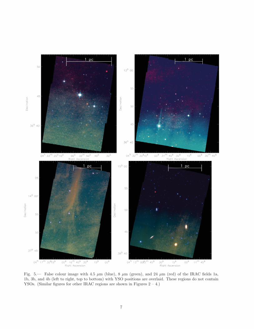
Fig. 5.— False colour image with 4.5 μm (blue), 8 μm (green), and 24 μm (red) of the IRAC fields 1a,1b, 3b, and 4b (left to right, top to bottom) with YSO positions are overlaid. These regions do not containYSOs. (Similar figures for other IRAC regions are shown in Figures 2 – 4.)

7

wavelength bands. The fundamental criteria useIRAC, MIPS and 2MASS data (Cutri et al. 2003)and are based on identification of infrared excessand brightness limits below which the probabil-ity of detection of external galaxies becomes high.The total number of sources is 704,045. In regionsobserved by both IRAC and MIPS, the YSOc se-lection follows that of Harvey et al. (2008). Werefer to these as IRAC+MIPS YSOcs. For objectswith upper limits on the MIPS 24 μm flux, we fol-low the method outlined by Harvey et al. (2006).We refer to these as IRAC-only YSOcs. In regionsobserved only by MIPS and not IRAC, we haveused the formalism of Rebull et al. (2007), exceptwe use a tighter 2MASS KS cut of [KS] < 13.5.This tighter magnitude cut removed objects thatwere similar in color and magnitude to others thathad already been eliminated. We further removegalaxies from the MIPS-only source list by includ-ing photometry from the Wide-field Infrared Sur-vey Explorer (WISE; Wright et al. 2010) and ap-plying color cuts suggested by Koenig et al. (2012)(see their Figure 7) and requiring the WISE Band2 magnitude criterion of [4.6] < 12. We refer tothese as MIPS-only YSOcs. Note that the MIPS-only YSOcs were not observed with IRAC, as op-posed to the IRAC-only YSOcs which were ob-served, but not detected, with MIPS.

Figure 6 shows the IRAC color-magnitude andcolor-color diagrams relevant for classifying IRAC-only sources. The different domains occupiedby stars, YSOcs, and other (e.g., extragalactic)sources are are shown.

For sources in regions observed by both IRACand MIPS, Figure 7 shows the color and mag-nitude boundaries used to remove sources thatare likely extragalactic. This identification isdone by comparing the observed fluxes and col-ors to results from the SWIRE extragalactic sur-vey (Surace et al. 2004). The sources in the AMCfield are compared to a control catalogue from theSWIRE dataset that is resampled to match oursensitivity limits and the extinction level derivedfor the AMC. (See Evans et al. 2007 for a completedescription.)

Finally, we vetted the YSOcs through individ-ual inspection of the Spitzer maps (and opticalimages where available), and determined that 24of the original 159 IRAC+MIPS YSOcs, 14 of theoriginal 17 IRAC-only YSOcs, and 56 (26 based

on WISE and other photometric criteria) of theoriginal 84 MIPS-only YSOcs were unlikely to beYSOs. Henceforth we refer to the list of vettedYSOcs, totalling 166, as YSOs to distinguish themfrom the raw unvetted list. While we have under-gone an extensive process to construct a list ofsources that are very likely to be YSOs, we stressthat these YSOs have not been confirmed spec-troscopically. Table 3 lists the final source countsfor objects in the observed fields. The IRAC andMIPS fluxes of the IRAC+MIPS and IRAC-onlyYSOs are listed in Table 4. The 70 μm fluxeshave been listed where available. (There are fewerYSOs with fluxes at 70 μm because of the lowersensitivity and, in some cases, the bright back-ground.) The fluxes of MIPS-only vetted YSOsare listed in Table 5 with their WISE and MIPSfluxes (and IRAC fluxes where available). In Ta-bles 4 and 5, we have noted which YSOs are inregions of low column density (NH2 < 5 × 1021

cm−2) according to the column density maps byHarvey et al. (2013), as these are more likely to becontaminants than YSOs in regions of high columndensity.

We compare our final YSO source list to thosefound for LkHα 101 in Gutermuth et al. (2009).All 103 YSOs in Gutermuth et al. (2009) are iden-tified as sources in our catalogue with positionsthat are within a couple tenths of an arcsecondagreement. Where this work and Gutermuth et al.(2009) provide fluxes, they agree at the shorterIRAC bands (IRAC1-3) typically within 0.05 –0.1 mag. At IRAC4 and MIPS1, the agreementis typically within 0.2 mag. These differences arewhat one might expect for PSF-fitting (used here)versus aperture fluxes (used by Gutermuth et al.2009) at wavelengths where there is substantialdiffuse emission. (Recall that we have incorpo-rated their dataset into our own.) Therefore nopreviously identified sources have been missed inthis study, and our measurements agree well withthose of Gutermuth et al. (2009). Note, however,that the different classification methods used inthis work and by Gutermuth et al. (2009) eachyield a different total number of YSOs in this re-gion; we have identified 42 YSOs whereas Guter-muth et al. (2009) identified 103. Our total breaksdown into 7 YSOs identified here that were notidentified by Gutermuth et al. (2009) and 35 YSOsshared between the two lists. (The c2d pipeline

8

Fig. 6.— IRAC colors of the sources in the the regions observed with IRAC. Stars are in blue; YSOs arein red; and “other sources” (e.g., galaxies) are in green. The boxed region on the right panel marks theapproximate domain of Class II sources identified by Allen et al. (2004).

identified 47 YSOcs that were listed as YSOs byGutermuth et al. (2009), but 12 were removed dur-ing the vetting process.) The major source of thisdiscrepancy is that we require 4 (or 5) band pho-tometry with S/N ≥ 3 in IRAC (and MIPS 24 μmbands) to identify YSO candidates. Such crite-ria are especially difficult to satisfy in the regionof bright and diffuse emission around LkHα 101.Therefore, our results do not contradict those inGutermuth et al. (2009), rather we believe thatthe stringent criteria used here have excluded someYSOs. We keep these criteria for consistency withother c2d and Spitzer GBS observations and anal-yses, but note the limitations in such a bright re-gion.

The diffuse emission problem is isolated to theimmediate vicinity of LkHα 101. To demonstratethis point, in Figure 8 we have plotted the locationof all the sources having an SED consistent withbeing a reddened stellar photosphere and an as-sociated dust component, which do not have S/N≥ 3 at all IRAC bands. The SEDs of these sourcesare classified as ‘star+dust’ in our catalogue. Ofthe 56 YSOs listed by Gutermuth et al. (2009)that were not identified as YSOs in this work, themajority of them (34 of 56) have a ‘star+dust’SED. There is a total of 465 ‘star+dust’ sources

without robust 4-band IRAC fluxes in the AMCfield. These sources are relatively evenly dis-tributed throughout the field, with the exceptionof a striking over-density at the center of LkHα 101compared to other IRAC regions. Therefore, webelieve this over-density is an effect of the diffi-culty in getting detections with S/N ≥ 3 across 4bands in the bright LkHα 101 region and not thatthere are significantly fewer YSOs than suggestedby Gutermuth et al. (2009).

Harvey et al. (2013) identified 60 YSOs in theAMC with Herschel/PACS, 49 of which are alsoidentified in this work. Four of these Spitzer -identified YSOs are members of pairs of YSOsthat are blended in the Herschel images. Her-schel is more sensitive to the rising- and flat-spectrum sources, i.e., of the other 45 Spitzer -identified YSOs that are also detected in the Her-schel maps, most (76%) are Class I/F objects, andthe remaining 24% are Class IIs.

3.2. YSO classification

The YSOs are classified according to the slopeof their SED in the infrared (see Evans et al. 2009for a description). The spectral index, α, is given

9

Fig. 7.— Color-magnitude and color-color diagrams for the AMC (left), the SWIRE dataset resampled tomatch our sensitivities and measured extinction (middle), and the full SWIRE dataset (right). The blackdash-dot lines show soft boundaries for YSO candidates whereas the red dash-dot lines show hard limits,fainter than which objects are not included as YSO candidates.10

Fig. 8.— Sources with SEDs consistent with a reddened stellar photosphere and a dust component (IRexcess) but for which detections with S/N ≥ 3 across all 4 IRAC bands, required to considered a YSOc,did not exist (see text). The positions of these sources are plotted against the 160 μm greyscale (colorbarunits are MJy sr−1). The striking over-density at the center of LkHα 101 compared to other IRAC+MIPSregions (marked by black lines) suggests that we are missing veritable YSOs in this region. The robust setof measurements required to identify whether a source is a likely YSO or background galaxy is difficult toattain in this region of very bright emission.

−3 −2 −1 0 1 2α

0

5

10

15

20

25

Num

ber

of

obje

cts

Class IClass FClass IIClass III

Fig. 9.— Left: Distribution of α values (the slope of the SED in the IR) used to determine the ‘class’ of theYSOs in the AMC. The vertical dotted lines mark the boundaries between the different classes as definedby Greene et al. (1994). Right: Pie chart for the AMC showing the percentage of sources in each SED class.Green is Class I; blue is Flat; red is Class II; and yellow is Class III (colors are the same as in Figure 18).

11

by

α ≡ d log(λS(λ))

d log(λ)(1)

and determined by fitting the photometry between2 μm and 24 μm. The distribution of α values isshown in Figure 9 along with the relative numberof YSOs in each SED class. The majority of YSOsidentified in the cloud are Class II objects (55%).The percentage of sources in each SED class forthe AMC is strikingly similar to that of Perseus(23%, 11%, 58%, and 8% for Class Is, Fs, IIs andIIIs, respectively; Evans et al. 2009).

Table 6 lists the breakdown of Class Is, Fs, andIIs for the AMC and other clouds in the GB andc2d surveys to estimate their relative ages. Wedid not include Class IIIs in this analysis sincethis population is typically incomplete in Spitzersurveys (e.g., see discussions in Harvey et al. 2008;Evans et al. 2009; Gutermuth et al. 2009) due totheir weak IR excess. This simplifies the compari-son to other clouds where the completeness limitsmay vary. We compared the ratio of Class Is andFs to Class IIs, NI+F/NII, for the different cloudpopulations in other GB and c2d surveys whichuse the same classification scheme. We also in-clude YSOs in the OMC identified with Spitzerby Megeath et al. (2012); since they use a dif-ferent classification scheme however, we have re-calculated the α values for their sample. TheClass I/F lifetime is relatively short compared tothe Class II lifetime, and therefore a higher ratioindicates a younger population (see discussion inEvans et al. 2009). The high number of Class Isand Fs suggests that the AMC is relatively youngcompared to other clouds.

Finally, we also compared the number of YSOsper square degree in the AMC (11.5 deg2)1 to thatin the OMC (14 deg2). The OMC is forming vastlylarger amounts of stars. It has 237 YSOs per deg2

whereas the AMC only has 13 YSOs per deg2, afactor of about 20 fewer. Even if we only comparethe number of YSOs in the OMC with 4 bandphotometry (as this was the source of the discrep-ancy between the total number of YSOs aroundLkHα 101 identified in this work and by Guter-muth et al. 2009, who use a similar identification

1Here we use the total coverage of IRAC + MIPS1, the fivebands used to identify YSOs. This differs from the over-lapping MIPS1, MIPS2 and MIPS3 coverage of 10.47 deg2

described in Section 1.

method to Megeath et al. 2012), this still suggeststhat there is at least a factor 15 more YSOs in theOMC than in the AMC. Despite the differences inidentification methods used for the OMC and forthe AMC, it is clear that the OMC is forming farmore stars than the AMC is. The YSOs in theOMC are also concentrated much more stronglythan the AMC, despite both clouds having com-parable sizes and masses. We note that Ladaet al. (2009) attribute the difference between theamount of star formation to the different amountsof material at high AV/column density.

4. Spectral Energy Distribution Modeling

Optical data of the YSOs were downloadedfrom the USNO NOMAD catalogue (Zacharias etal. 2004). SEDs of the YSOs are shown in Fig-ures 10 and 11 (Class Is and Class Fs), 12 – 14(Class IIs) and 15 (Class IIIs). We were able toperform relatively detailed modelling of the stel-lar and dust components of the Class II and ClassIII sources (YSOs which are not heavily obscuredby dust). The luminosities of sources in the earlierclasses are presented in Dunham et al. (2013). Themajority of the Class II and Class III sources arelikely in the physical stage where the stellar sourceand circumstellar disk are no longer enshroudedby a circumstellar envelope. We note that the ob-served “class” does not always correspond to theassociated physical stage of the YSO (see discus-sion in Evans et al. 2009) and that some Class IIsmay be sources, viewed pole-on, with circumstel-lar envelopes that are only beginning to dissipate.Conversely, an edge-on disk without an envelopecould look like a Class I object.

Our SED modelling methods follow those usedby Harvey et al. (2007) (and similar works since,e.g., Merın et al. 2008, Kirk et al. 2009) to modelthe SEDs. The stellar spectrum of a K7 starwas fit to the SEDs by normalizing it to the de-reddened fluxes in the shortest available IR bandof J, K or IRAC1. We use the extinction law ofWeingartner & Draine (2001) with RV= 5.5 tocalculate the de-reddened fluxes. The AV valuewas estimated by matching the de-reddened fluxeswith the stellar spectrum. In eight cases, we usedan A0 spectrum when the K7 spectrum was unableto produce a reasonable fit. The use of only twostellar spectra is of course over-simplified; how-

12

Fig. 10.— SEDs of Class I and Flat sources. The YSO ID, from Tables 4 and 5, is shown in the upper rightof each panel along with the Class (I or F) of the YSO.

13

Fig. 11.— continued from Figure 10.

14

Fig. 12.— SEDs of Class II sources. The YSO ID, from Tables 4 and 5, is shown in the upper right ofeach panel. The observed fluxes are plotted with unfilled circles. The de-reddened fluxes are plotted withfilled circles. The grey line plots the model stellar spectrum fit to the shorter wavelengths. The black lineshows the median SED of T Tauri stars in Taurus (with error bars denoting quartiles of the distribution,D’Alessio et al. 1999) normalized to the B band flux and J band flux of the K7 and A0 stellar spectrummodels, respectively.

15

Fig. 13.— continued from Figure 12.

16

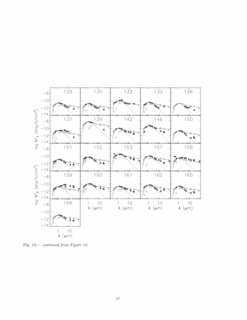
Fig. 14.— continued from Figure 12.

17

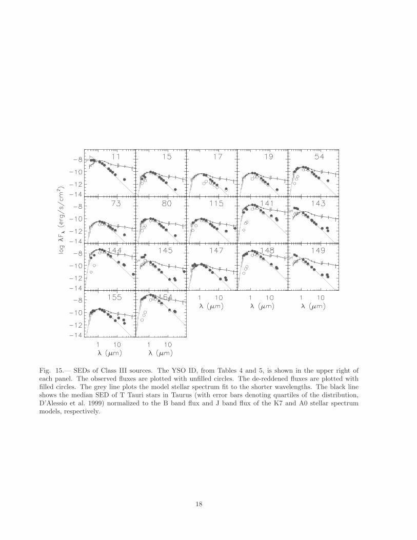
Fig. 15.— SEDs of Class III sources. The YSO ID, from Tables 4 and 5, is shown in the upper right ofeach panel. The observed fluxes are plotted with unfilled circles. The de-reddened fluxes are plotted withfilled circles. The grey line plots the model stellar spectrum fit to the shorter wavelengths. The black lineshows the median SED of T Tauri stars in Taurus (with error bars denoting quartiles of the distribution,D’Alessio et al. 1999) normalized to the B band flux and J band flux of the K7 and A0 stellar spectrummodels, respectively.

18

ever, it produces adequate results for the purposesof this study. More exact spectral typing is diffi-cult with only the photometric data presented hereand the uncertainties in AV. We nevertheless ob-tain a broad overview of the disk population withthe applied assumptions. Tables 7 and 8 list thestellar spectrum, the AV value, and stellar lumi-nosity (Lstar) used for the stellar models of eachsource’s SED for the Class II and Class III YSOs,respectively.

4.1. Second order SED parameters αexcess andλturnoff

The first order SED parameter α is used as aprimary diagnostic of the excess and circumstellarenvironment and to separate the YSOs into differ-ent “classes” (§ 3.2). Once we have a model of thestellar source, however, we are able to character-ize the circumstellar dust better. For each sourcewe determined the values of αexcess and λturnoff

defined by Cieza et al. (2007) and Harvey et al.(2007) and used in many works since. λturnoff isthe longest measured wavelength before an excessgreater than 80% of the stellar model is observed.If no excess > 80% is observed, than λturnoff isset to 24 μm. αexcess is the slope of the SED atwavelengths longward of λturnoff . αexcess is not cal-culated for YSOs with λturnoff = 24 μm as thereare not enough data points to determine the slopeof the excess. These parameters provide a bet-ter characterization of the excess since α can in-clude varying contributions from the stellar anddust components.

Figure 16 shows the distribution of αexcess andλturnoff for the Class IIs and Class IIIs. Class IIand Class III YSOs with long λturnoff and posi-tive αexcess (YSOs 2, 24, 58, 64, 74, 102, 108, 113,115, and 133 in the 8 μm bin and YSOs 145, 150,162, and 165 in the 12 μm bin of Figure 16) aregood classical transition disk candidates; the lackof near-IR excess but large mid-IR excess is a signof a deficit of material close to the star within asubstantial disk. Cieza et al. (2012) have recentlydone a study on the transition disks in the AMC,Perseus and Taurus and identify six transition diskcandidates in the AMC, three of which are also inour list of candidates (YSOs 58, 102 and 115). Oftheir remaining candidates, two were debris-likedisks (YSOs 11 and 54) and the other was notidentified in our YSO list. The larger distribu-

2 4 6 8 10 12 14

λturnoff

(μm)

−3

−2

−1

0

1

2

αexcess

Class IIs

Class IIIs

Fig. 16.— Distribution of αexcess and λturnoff forClass II and Class III sources. The Class IIIs withλturnoff= 24 μm (IDs 15, 19, 80, and 148) are notshown as those sources typically do not have excessmeasured across a wide enough range to calculatereliable values of αexcess.

tion of αexcess for sources with longer λturnoff isconsistent with distributions found for other diskpopulations (e.g., Cieza et al. 2007; Alcala et al.2008; Harvey et al. 2008; Merın et al. 2008).

4.2. Disk luminosities

Figure 17 shows the ratio of the disk luminosi-ties to stellar luminosities for the Class II andClass III sources. The disk luminosity is the in-tegral of the observed excesses. (The excess at agiven wavelength is calculated by subtracting theflux of the stellar model at that wavelength fromthe observed flux). The distribution of Ldisk/Lstar

for Class II and III sources in the AMC is simi-lar to that found for other c2d and GB surveyswith Spitzer (Serpens: Harvey et al. 2007, IC5146: Harvey et al. 2008, Chameleon II: Alcalaet al. 2008, Lupus: Merın et al. 2008, and theCepheus Flare: Kirk et al. 2009). We find theClass III sources in the regions typically occupiedby sources with passive disks and debris disks (e.g.,0.02 < Ldisk/Lstar< 0.08 for passive disks; Kenyon& Hartmann 1987). The low disk luminosity maybe attributable to the lack of mid-IR excess atIRAC wavelengths in these sources’ SEDs.

19

−3 −2 −1 0 1 2

log Ldisk/Lstar

0

5

10

15

20

Num

ber

of

obje

cts

Debris Passive Accreting

All

Class IIs

Class IIIs

Fig. 17.— The ratio of the disk luminosity tothe stellar luminosity for Class II and Class IIIsources. Also shown are the typical boundariesfound for accreting disks, passive disks and debrisdisks (Kenyon & Hartmann 1987).

4.3. Questionable Class III sources

It is possible that some of the Class III sourcesidentified here are field giants. Oliveira et al.(2009) followed up on 150 Spitzer identified YSOsin Serpens and obtained 78 optical spectra withsufficient signal-to-noise. They showed that therewere at least 20 giant contaminants in this list, 18of which were identified as Class III sources. Themore scattered spatial distribution of Class IIIsthroughout the AMC is consistent with this ideathat they are contaminants. Additionally, five ofour Class III objects (YSOs 11, 141, 144, 148, 164)have very high luminosities (> 100 L�). Four ofthese objects (YSOs 141, 144, 148, 164), as wellas YSO 149 which is not of particularly high lu-minosity, are quite removed from the areas of highextinction towards the AMC (see Figure 18 in thefollowing section) and regions of low column den-sity (NH2 < 5× 1021 cm−2, see § 3.1).

5. Spatial Distribution of Star Formation

The spatial distribution of IRAC/MIPS-identifiedYSOs by class is shown in Figure 18. A close-up ofthe region surrounding the LkHα 101 cluster andthe cluster extension along the filament is also

included so the relatively densely clustered YSOscan be better distinguished. Figure 18 shows thatthe bulk of star formation in the AMC has beenconcentrated in this southern region of the cloud;the majority of the identified YSOs (79%) are inthis area. (Note that the number of YSOs in thatregion is a lower limit as it is likely that a signifi-cant number of YSOs in the LkHα 101 region arenot identified, see discussion at the end of § 3.1.)

5.1. Identification of YSO groups

We performed a clustering analysis on the iden-tified Class I, F, and II sources in the AMC to iden-tify the densest regions of YSOs and the largestgroups. The details of the analysis are describedin Masiunas et al. (2012). We omit the Class IIIsources from the analysis to avoid the risk of in-cluding field giants (see for example § 4.3). Weperformed a minimum spanning tree (MST) anal-ysis to identify groups of YSOs within the re-gion. This analysis connects YSOs by the mini-mum distance to the next YSO to form a “branch”(Cartwright & Whitworth 2004). Figure 19 showsthe cumulative distribution function (CDF) of thebranch lengths between YSOs. This is used to de-termine the MST critical branch length, Lcrit, thatdefines the transition between the branch lengthsin the denser regions to the branch lengths in thesparser regions (Gutermuth et al. 2009). ThereforeLcrit is based on relative over densities of objects.We measure an Lcrit of 210

′′ for the AMC. Groupmemberships are defined by members which are allconnected by branches of lengths less than Lcrit.The boundary of a group is defined where thebranch length between adjacent sources exceedsLcrit. Figure 20 shows that we have extractedfour groups with 10 or more members (markedby colored convex hulls) and three groups with5–9 members (marked with magenta circles). Ta-ble 9 lists the properties of these groups. The po-sition of the group is given by its geometric center.The group’s effective radius, Reff , defines the ra-dius of a circle with the same area as the convexhull containing the group members. The maxi-mum radial distance to a member from the me-dian position gives Rcirc, therefore a circle withthis radius would contain all group members. Fi-nally, the elongation of the group is determinedby comparing Rcirc to Reff and represented by theaspect ratio, Rcirc

2/Reff2. The MST analysis on

20

Fig. 18.— Left: The positions of YSOs and IRAC fields in Auriga. The greyscale is the MIPS 160μm map(colorbar units are MJy sr−1) and the YSOs are marked according to their classification: green circles denoteClass Is; blue +s denote Class Fs; red ×s denote Class IIs; yellow triangles denote Class IIIs. The magentadiamonds mark the Class III sources of high luminosities that are likely contaminants (see § 4.3). IRACfields are outlined in black and labelled. (Note that some YSOs fall beyond the 160 μm coverage because itis slightly offset from the 24 μm coverage that is used for YSO identification.) Right: Close-up of the regionaround LkHα 101. The greyscale is the log (base 10) of the flux (colorbar units are log(MJy sr−1)). Thecentre of the field is entirely saturated. As is evident, there are some YSOs outside the IRAC coverage area.This list of MIPS-only YSOs has been trimmed by using WISE data to remove more objects that are likelybackground galaxies.

21

the full cloud recovers the clustering surroundingLkHα 101. The cluster subtends a larger area thanthat measured in Gutermuth et al. (2009) confirm-ing their claim that there was star formation ex-tended beyond their field of view. The star for-mation is mostly extended along the North-Southdirection of the cluster and therefore we measurea more elongated group than measured by Guter-muth et al. (2009). This is still the largest groupin the AMC in terms of area and the number ofmembers.

Fig. 19.— Cumulative distribution function(CDF) of MST branch lengths (asterisks). Thesolid lines represent linear fits to each end of theCDF. The dot-dash line marks Lcrit where thesolid lines meet. The solid lines follow the CDFin the dense regions (steep line) and the sparserregions (shallow line).

As discussed in § 3.1, our analysis is likely tohave underestimated the number of YSOs in theregion around LkHα 101. To check the consistencyof our analysis with Gutermuth et al. (2009), weran the MST analysis on both YSO lists within theGutermuth et al. (2009) area of 4-channel IRACcoverage. This leaves us with 41 of the YSOs pre-sented here and 102 of those presented in Guter-muth et al. (2009). (There is one bright YSOin Gutermuth et al. 2009 that lies just outsidetheir 4-channel IRAC coverage to the south. It

was only observed at IRAC1 and IRAC3.) Weget an Lcrit of 120′′ for our cropped list of YSOsand an Lcrit of 73′′ for the cropped Gutermuthet al. (2009) YSO list. (Note that running theanalysis on the cropped field, which is dense com-pared to the rest of the cloud, yields a smallerLcrit than when the analysis is run on the wholecloud. This is expected as Lcrit is based on overdensities, as discussed above.) The ratio of theLcrit values for the two YSO lists (73/120 = 0.61)agrees with our expectation that it should scalewith the square-root of the density, and hence thecropped YSO count (

√102/41 = 0.63). There-

fore we report that the derived properties are con-sistent with those measured by Gutermuth et al.(2009). (Differences are expected as shown byGutermuth et al. (2009) with their comparisonsamong several shared regions.) However, the miss-ing YSOs at the centre of the cluster complicateany further comparison their results.

5.2. Comparison of grouped and non-grouped YSOs

We find 76% (113 of the 149) of the ClassIs, Class Fs, and Class IIs are found in groups.Rather than compare the class fractions, given byNI+F/NII in Table 9, we directly compare the un-derlying distribution of α to determine whetherthe distribution of YSOs within groups is consis-tent with the whole cloud. We get the same resultfor each group: a KS test on the α distributionof the group and the α distribution of the wholecloud shows that we cannot reject the hypothe-sis that they are drawn from the same sample (p-values > 0.13). (We also did a KS test for eachgroup with the extended population and found thesame result.)

Similarly, we compared the properties of diskswithin groups and those not in groups by perform-ing a KS test on the distributions of disk luminosi-ties (p-value of 0.08), αexcess (p-value of 0.9), andλturnoff (p-value of 0.9) and find no evidence thatthe two populations are drawn from different par-ent populations.

6. Summary

We observed the AMC with IRAC and MIPSaboard the Spitzer Space Telescope and identify138 YSOs in the cloud. As our IRAC coverage is

22

segmented, we complemented our more contiguousMIPS coverage with WISE data to further elimi-nate galaxies from the sample, leaving 28 MIPS-only YSOs remaining, bringing the total numberof YSOs in the AMC to 166. We classified theYSOs based on the spectral slope of their SEDsbetween 2 μm and 24 μm and find 37 Class I ob-jects, 21 Class F objects (flat spectrum sources),91 Class II objects, and 17 Class III objects. Thehigh fraction of Class Is and Class Fs suggeststhat the AMC is relatively unevolved comparedto other star-forming clouds. Despite the simi-larity in cloud properties between the AMC andthe OMC, there is a distinct difference in the starformation properties. The star formation in theAMC is also concentrated along its filament, how-ever, it is also forming a factor of about 20 fewerstars than the OMC. Lada et al. (2009) find thatthere is much less material at high density in theAMC than in the OMC and attribute the differ-ence in star formation to this. Further studiesof the star formation and YSO population in theAMC are needed to highlight the differences of thetwo clouds given their similar age.

We modelled the SEDs of the Class II and ClassIII sources and their excesses by first fitting a K7stellar spectrum to the optical and near-IR fluxes.The spectrum is normalized to the 2MASS flux (orthe IRAC1 flux when 2MASS is unavailable) andwe use an AV value to match the spectrum of thestellar model to the de-reddened observed opticalfluxes. An A0 stellar spectrum is used in the eightcases where a K7 spectrum is unable to provide areasonable fit. Fitting a stellar spectrum allows usto measure the disk luminosities and characterizethe excess. The excesses of the Class II and ClassIII sources were further parameterized by λturnoff ,the longest wavelength before an excess greaterthat 80% is measured, and αexcess, the slope of theSED at wavelengths longward of λturnoff . λturnoff

is a useful tracer for the proximity of dust to thestar and consequently we identify fourteen classi-cal transition disk candidates.

The bulk of the star formation in the AMCis in the southern region of the cloud. We in-cluded a clustering analysis to quantify the dens-est areas of star formation and to identify groupswithin the cloud. We find four groups with 10 ormore members all in the region around LkHα 101and its adjoining filament. We find three smaller

groups with 5 – 9 members scattered through-out the cloud. The largest group is that aroundLkHα 101 and contains 49 members. We notethat there are likely even more YSOs in this groupsince our YSO identification criteria of S/N ≥ 3 inIRAC1-4 and MIPS1 are difficult to attain in thisbright region.

We thank the referee whose comments and sug-gestions greatly helped improve the paper andits clarity. H.B.F gratefully acknowledges re-search support from an NSERC Discovery Grant.This research made use of APLpy, an open-source plotting package for Python hosted athttp://aplpy.github.com This research made useof Montage, funded by the National Aeronauticsand Space Administration’s Earth Science Tech-nology Office, Computation Technologies Project,under Cooperative Agreement Number NCC5-626 between NASA and the California Instituteof Technology. Montage is maintained by theNASA/IPAC Infrared Science Archive.

REFERENCES

Alcala, J. M., Spezzi, L., Chapman, N., et al. 2008,ApJ, 676, 427

Allen, L. E., Calvet, N., D’Alessio, P., et al. 2004,ApJS, 154, 363

Cartwright, A., & Whitworth, A. P. 2004, MN-RAS, 348, 589

Cieza, L., Padgett, D. L., Stapelfeldt, K. R., et al.2007, ApJ, 667, 308

Cieza, L. A., Schreiber, M. R., Romero, G. A.,et al. 2012, ApJ, 750, 157

Cutri, R. M., Skrutskie, M. F., van Dyk, S., et al.2003, 2MASS All Sky Catalog of point sources.,ed. Cutri, R. M., Skrutskie, M. F., van Dyk, S.,Beichman, C. A., Carpenter, J. M., Chester,T., Cambresy, L., Evans, T., Fowler, J., Gizis,J., Howard, E., Huchra, J., Jarrett, T., Kopan,E. L., Kirkpatrick, J. D., Light, R. M., Marsh,K. A., McCallon, H., Schneider, S., Stiening,R., Sykes, M., Weinberg, M., Wheaton, W. A.,Wheelock, S., & Zacarias, N.

D’Alessio, P., Calvet, N., Hartmann, L., Lizano,S., & Canto, J. 1999, ApJ, 527, 893

23

Dobashi, K., Uehara, H., Kandori, R., et al. 2005,PASJ, 57, 1

Dunham, M. M., Arce, H. G., Allen, L. E., et al.2013, AJ, 145, 94

Evans, N. J., Dunham, M. M., Jørgensen, J. K.,et al. 2009, ApJS, 181, 321

Evans, II, N. J., Allen, L. E., Blake, G. A., et al.2003, PASP, 115, 965

Evans, II, N. J., Harvey, P. M., Dunham, M. M.,et al. 2007

Fazio, G. G., Hora, J. L., Allen, L. E., et al. 2004,ApJS, 154, 10

Greene, T. P., Wilking, B. A., Andre, P., Young,E. T., & Lada, C. J. 1994, ApJ, 434, 614

Gutermuth, R. A., Megeath, S. T., Myers, P. C.,et al. 2009, ApJS, 184, 18

Harvey, P., Merın, B., Huard, T. L., et al. 2007,ApJ, 663, 1149

Harvey, P. M., Chapman, N., Lai, S.-P., et al.2006, ApJ, 644, 307

Harvey, P. M., Huard, T. L., Jørgensen, J. K.,et al. 2008, ApJ, 680, 495

Harvey, P. M., Fallscheer, C., Ginsburg, A., et al.2013, ApJ, 764, 133

Jørgensen, J. K., Harvey, P. M., Evans, II, N. J.,et al. 2006, ApJ, 645, 1246

Kenyon, S. J., & Hartmann, L. 1987, ApJ, 323,714

Kirk, J. M., Ward-Thompson, D., Di Francesco,J., et al. 2009, ApJS, 185, 198

Koenig, X. P., Leisawitz, D. T., Benford, D. J.,et al. 2012, ApJ, 744, 130

Lada, C. J., Lombardi, M., & Alves, J. F. 2009,ApJ, 703, 52

Lynds, B. T. 1962, ApJS, 7, 1

Masiunas, L. C., Gutermuth, R. A., Pipher, J. L.,et al. 2012, ApJ, 752, 127

Megeath, S. T., Gutermuth, R., Muzerolle, J.,et al. 2012, AJ, 144, 192

Merın, B., Jørgensen, J., Spezzi, L., et al. 2008,ApJS, 177, 551

Oliveira, I., Merın, B., Pontoppidan, K. M., et al.2009, ApJ, 691, 672

Peterson, D. E., Caratti o Garatti, A., Bourke,T. L., et al. 2011, ApJS, 194, 43

Rebull, L. M., Stapelfeldt, K. R., Evans, II, N. J.,et al. 2007, ApJS, 171, 447

Rieke, G. H., Young, E. T., Engelbracht, C. W.,et al. 2004, ApJS, 154, 25

Surace, J. A., Shupe, D. L., Fang, F., et al. 2004,VizieR Online Data Catalog, 2255, 0

Ungerechts, H., & Thaddeus, P. 1987, ApJS, 63,645

Weingartner, J. C., & Draine, B. T. 2001, ApJ,548, 296

Werner, M. W., Roellig, T. L., Low, F. J., et al.2004, ApJS, 154, 1

Wolk, S. J., Winston, E., Bourke, T. L., et al.2010, ApJ, 715, 671

Wright, E. L., Eisenhardt, P. R. M., Mainzer,A. K., et al. 2010, AJ, 140, 1868

Young, K. E., Harvey, P. M., Brooke, T. Y., et al.2005, ApJ, 628, 283

This 2-column preprint was prepared with the AAS LATEXmacros v5.2.

24

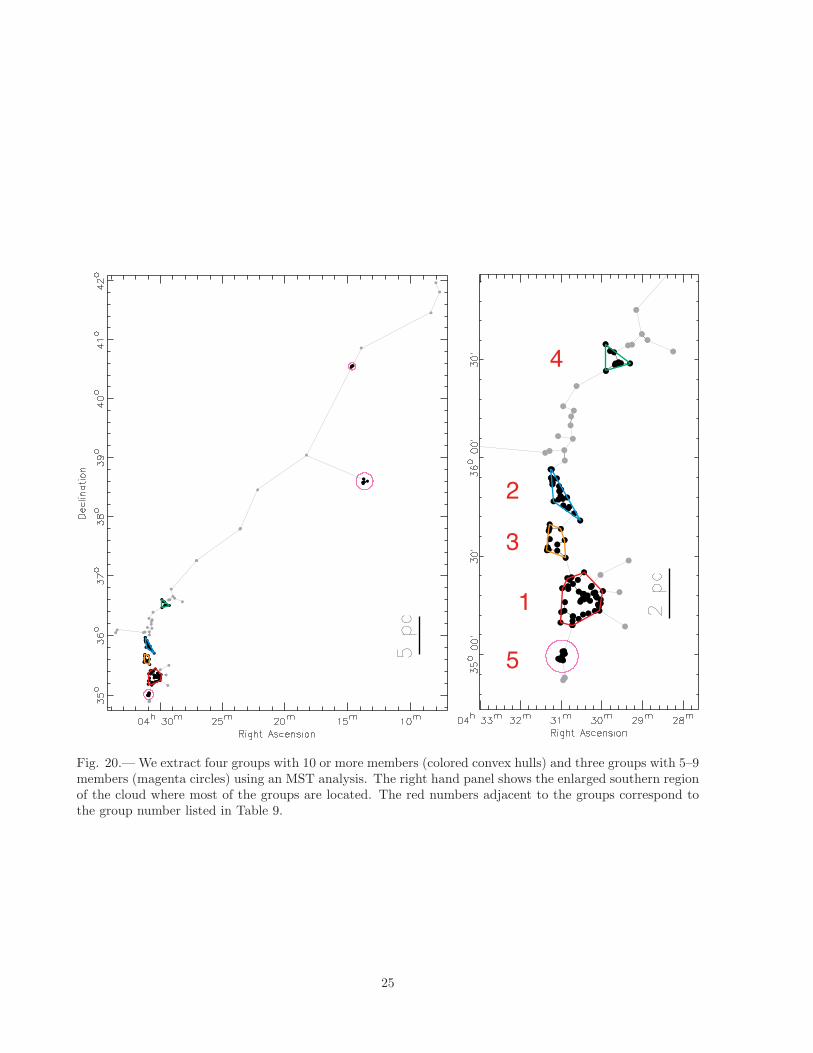
Fig. 20.— We extract four groups with 10 or more members (colored convex hulls) and three groups with 5–9members (magenta circles) using an MST analysis. The right hand panel shows the enlarged southern regionof the cloud where most of the groups are located. The red numbers adjacent to the groups correspond tothe group number listed in Table 9.

25

Table 1

Summary of IRAC Observations

IRAC Sub-region Size AOR Sub-region ID AOR Key (1st epoch, 2nd epoch)(sq. deg.)

AUR 1a 0.3 × 0.2 auri irac6b 19972096, 19971584AUR 1b 0.4 × 0.3 auri irac6 20014336, 20014080AUR 1c 0.9 × 0.3 auri irac7 19980544, 19980288

auri irac7b 19984384, 19984128AUR 1d 0.3 × 0.2 non-GB data 03654144AUR 1e 0.3 × 0.3 auri irac8 20013312, 20013056AUR 2a 1.3 × 1.4 auri irac3 19983360, 19983104

auri irac4 20016640, 20016384auri irac5 19981824, 19981568auri irac5b 19956480, 19956224

AUR 2b 0.4 × 0.3 auri irac2 20018432, 20017920AUR 3a 0.8 × 0.9 auri irac1 19984640, 19967744

auri irac9 19978240, 19977984AUR 3b 0.4 × 0.3 auri irac9b 20012288, 20011776

auri irac9c 19976960, 19976192AUR 4a 0.4 × 0.7 auri irac10 19993344, 19993088

auri irac10b 19988992, 19988736AUR 4b 0.3 × 0.3 auri irac11 19961088, 19960832AUR 5 0.3 × 0.3 auri irac12 19992576, 19992064AUR NORTH 0.5 × 0.3 auri irac13 19960320, 19959808

Table 2

Summary of MIPS Observations

MIPS Sub-region Size AOR Key(sq. deg)

AUR 1 1.2 × 3.2 20019712,19983872,20019456,19983616AUR 2 1.6 × 2.6 20017152,19982336,20016896,19982080AUR 3 1.0 × 2.0 20015360,20014848AUR 4 1.4 × 2.2 19981312,19979520,19981056,19979008AUR 5 0.5 × 1.9 20013824,20013568AUR NORTH 0.5 × 1.9 20011520

26

Table 3

Sources in the AMC Field

Sources Number

Total 704045YSO 166Galc 322Stellar 325792MASS 87745Zero a 247257Something else 335976

aSources that do not havedetections in the combinedepochs data in any of the2MASS, IRAC or MIPSbands. (It may have beendetected in one or both of theepochs at different bands.)

27

Table 4

YSOs in the AMC Based on IRAC and MIPS

3.6 μm 4.5 μm 5.8 μm 8.0 μm 24.0 μm 70.0 μmID Name Class α (mJy) (mJy) (mJy) (mJy) (mJy) (mJy)

1N 04012455+4101490 I 2.04 0.50±0.03 4.06±0.20 7.94±0.38 8.49±0.41 352± 32 8410± 9652N 04013436+4111430 II -1.00 10.5± 0.5 9.66±0.46 8.99±0.44 7.65±0.36 14.7± 1.4 288± 303 04100064+4002361 II -0.31 2.64±0.13 3.63±0.18 4.50±0.22 5.16±0.25 9.66±0.93 · · ·4 04100263+4002482 I 0.98 0.60±0.04 0.99±0.05 0.96±0.06 0.91±0.06 49.3± 4.6 · · ·5 04100562+4002386 II -0.79 3.46±0.20 3.65±0.20 3.74±0.20 4.18±0.20 3.51±0.68 · · ·6 04100841+4002244 I 1.70 18.6± 2.8 53.3± 3.0 119± 6 237± 11 4770± 470 24600± 35507 04101116+4001262 I 1.99 0.066±0.006 0.35±0.02 0.34±0.03 0.27±0.04 41.1± 3.8 · · ·8 04104051+3805004 II -0.78 12.9± 0.6 11.5± 0.5 11.6± 0.6 14.9± 0.7 25.1± 2.3 64.0±13.19 04104163+3808058 II -0.32 13.9± 0.7 14.1± 0.9 14.3± 1.0 18.9± 1.6 226± 75 · · ·10 04104109+3807545 I 2.03 1280± 78 2150± 132 4330± 244 5530± 304 11000± 2200 · · ·11 04104211+3805599 III -2.26 341± 25 210± 12 151± 9 87.1± 4.4 43.9± 4.2 · · ·12 04104761+3803338 II -0.87 6.21±0.32 6.14±0.33 6.11±0.30 7.42±0.37 7.18±0.70 · · ·13 04104916+3804458 II -0.49 44.1± 2.2 46.3± 2.2 57.0± 2.7 85.0± 4.1 123± 11 253± 2614 04194467+3811219 F -0.07 4.54±0.23 5.62±0.27 7.26±0.36 10.2± 0.5 22.5± 2.1 · · ·15 04205246+3806358 III -2.42 14.5± 0.7 10.1± 0.5 7.13±0.35 4.33±0.23 1.08±0.17 · · ·16 04213795+3734418 II -0.85 284± 14 387± 20 443± 21 432± 20 223± 20 5530± 123017 04213808+3735409 III -1.64 1.88±0.09 1.71±0.08 1.29±0.07 0.77±0.06 0.92±0.20 · · ·18 04214080+3733590 I 1.99 1.12±0.06 4.07±0.20 10.2± 0.5 26.1± 1.2 241± 22 945± 11219 04244934+3716464 III -2.27 6.19±0.30 4.14±0.20 3.05±0.16 1.89±0.11 0.91±0.20 · · ·20 04253848+3707012 I 1.43 0.60±0.03 1.04±0.08 1.95±0.13 4.50±0.25 59.1± 5.5 1350± 15221 04253979+3707082 F -0.01 254± 12 485± 25 671± 33 744± 39 727± 68 1160± 15722 04275080+3631264 II -0.86 7.15±0.35 6.93±0.34 6.45±0.32 7.28±0.35 11.4± 1.1 · · ·23 04275826+3633265 II -1.03 1.72±0.08 1.59±0.08 1.52±0.08 1.54±0.09 2.08±0.30 · · ·24 04280289+3640586 II -0.37 1.81±0.09 1.59±0.08 1.39±0.08 1.23±0.08 12.5± 1.2 · · ·25 04281515+3630286 F 0.25 7.28±0.36 10.4± 0.5 13.8± 0.7 18.3± 0.9 61.3± 5.7 75.4±13.826 04282116+3624478 II -0.83 6.30±0.31 5.79±0.28 5.20±0.26 5.40±0.26 11.8± 1.1 · · ·27 04282136+3630215 II -1.09 2.93±0.14 2.60±0.13 2.63±0.14 2.50±0.13 2.55±0.30 · · ·28 04283509+3625064 I 0.88 10.7± 0.5 27.5± 1.3 45.8± 2.2 62.1± 2.9 237± 21 840± 9229 04283789+3624553 II -0.63 124± 6 140± 6 161± 8 188± 9 204± 18 1240± 12330 04283856+3625289 I 1.14 0.83±0.04 1.56±0.08 1.56±0.09 1.99±0.11 143± 13 896± 9631 04284335+3625117 II -0.44 9.32±0.45 9.36±0.45 9.92±0.48 15.7± 0.7 30.1± 2.8 · · ·32 04284367+3628393 I 1.16 1.34±0.07 3.58±0.18 4.01±0.19 4.01±0.20 192± 17 2170± 24433 04284443+3624456 F 0.12 1.73±0.08 2.55±0.12 3.46±0.17 5.78±0.28 10.4± 1.0 · · ·34 04284958+3629107 I 0.47 3.08±0.15 5.70±0.27 7.60±0.37 9.14±0.44 51.0± 4.7 93.2±16.935 04285530+3631225 I 1.18 17.9± 0.9 51.0± 2.4 83.1± 4.0 109± 5 752± 70 4290± 47636∗ 04285911+3623112 II -1.23 30.7± 1.5 28.5± 1.4 24.9± 1.2 27.2± 1.3 21.9± 2.0 · · ·37 04293901+3516105 II -1.00 37.0± 2.1 35.0± 1.8 29.5± 1.6 41.0± 2.1 36.8± 3.5 · · ·38 04294001+3521089 I 0.51 22.7± 1.1 28.1± 1.4 50.6± 2.5 160± 8 147± 14 · · ·39 04294358+3513386 II -0.86 18.8± 0.9 17.9± 0.9 17.8± 0.9 23.0± 1.1 21.0± 2.1 · · ·40 04294421+3512300 F -0.21 8.89±0.43 9.39±0.46 10.2± 0.5 16.2± 0.8 44.2± 4.1 · · ·41 04294728+3510192 II -0.54 10.9± 0.5 11.4± 0.5 13.6± 0.7 21.1± 1.0 16.6± 1.6 · · ·42 04294742+3511335 II -1.37 5.59±0.27 4.66±0.22 4.19±0.22 3.99±0.20 2.70±0.36 · · ·43 04294854+3512125 II -0.75 3.21±0.15 4.47±0.22 3.54±0.18 5.09±0.25 4.13±0.50 · · ·44 04294921+3514227 F -0.24 62.6± 3.2 74.9± 3.7 76.9± 3.7 94.9± 4.7 196± 18 · · ·45 04294961+3514438 II -0.51 8.80±0.44 11.0± 0.5 9.26±0.46 9.66±0.48 27.6± 2.8 · · ·46 04295084+3515579 F -0.11 33.3± 1.7 43.1± 2.2 45.1± 2.2 65.0± 3.1 177± 17 · · ·47 04295101+3515475 I 0.74 5.80±0.30 8.90±0.44 15.3± 0.8 31.1± 1.5 98.6±11.0 · · ·48 04295346+3515485 F -0.26 17.7± 0.9 17.9± 0.9 21.0± 1.1 31.5± 1.9 79.0± 8.4 · · ·49 04295415+3510216 F 0.08 2.44±0.12 4.56±0.22 6.10±0.32 8.85±0.44 16.5± 1.6 · · ·

28

Table 4—Continued

3.6 μm 4.5 μm 5.8 μm 8.0 μm 24.0 μm 70.0 μmID Name Class α (mJy) (mJy) (mJy) (mJy) (mJy) (mJy)

50 04295479+3518025 II -0.32 29.6± 1.5 32.0± 1.6 35.0± 1.8 51.2± 3.4 135± 12 · · ·51 04295627+3517429 I 0.61 10.0± 0.5 17.4± 0.9 23.1± 1.3 28.3± 2.6 57.7±11.2 · · ·52 04295976+3513342 II -0.81 139± 8 128± 6 114± 5 151± 8 195± 18 · · ·53∗ 04300016+3603227 II -1.05 12.2± 0.6 11.4± 0.5 10.6± 0.5 11.8± 0.6 12.9± 1.2 · · ·54 04300114+3517246 III -1.93 75.7± 4.0 48.0± 2.5 30.8± 1.6 22.9± 1.5 26.5± 3.4 · · ·55 04300263+3515143 II -1.00 53.3± 2.7 44.5± 2.2 41.0± 2.1 46.4± 2.7 66.4± 7.3 · · ·56 04300363+3514201 I 0.75 8.19±0.57 12.5± 0.6 17.6± 1.3 31.4± 4.1 37.4±11.2 · · ·57 04300423+3509459 II -1.17 2.06±0.10 1.85±0.09 1.73±0.10 2.02±0.12 1.33±0.26 · · ·58∗ 04300425+3522238 II -0.62 6.47±0.37 4.25±0.21 3.23±0.25 2.69±0.60 24.8± 2.5 688± 11859 04300743+3514579 II -0.88 124± 6 127± 6 121± 5 139± 7 137± 13 · · ·60 04300773+3515484 II -0.77 24.3± 1.2 24.6± 1.2 22.2± 1.3 27.6± 2.0 53.8±12.8 · · ·61 04300825+3514100 I 0.46 9.62±0.48 14.9± 0.7 19.3± 1.1 27.1± 2.0 119± 13 · · ·62 04300874+3514375 II -0.84 107± 5 105± 5 105± 5 127± 8 158± 38 · · ·63 04300951+3514403 I 0.81 8.53±0.51 12.5± 0.6 16.6± 1.6 24.6± 5.2 334± 33 · · ·64∗ 04300980+3540355 II -0.89 3.61±0.18 2.96±0.14 2.46±0.13 2.47±0.13 8.30±0.79 57.0± 9.065 04300991+3515539 II -0.94 56.8± 3.2 48.4± 2.9 44.8± 2.8 63.2± 4.0 139± 42 · · ·66 04301234+3509346 II -0.99 7.18±0.35 7.73±0.37 7.17±0.35 6.30±0.30 7.86±0.76 · · ·67 04301309+3513586 II -0.90 107± 7 93.5± 4.8 81.6± 4.6 93.2± 7.1 153± 15 · · ·68 04301453+3513326 II -0.39 81.4± 7.7 96.1± 4.9 96.3± 5.0 108± 7 160± 27 · · ·69 04301474+3520143 II -0.60 136± 10 146± 8 166± 8 191± 11 197± 19 · · ·70 04301495+3600085 I 1.77 0.22±0.01 1.07±0.05 2.61±0.14 4.45±0.22 48.2± 4.5 137± 1671 04301576+3556578 I 0.40 996± 51 1450± 79 2080± 103 2910± 163 5500± 1100 · · ·72∗ 04301627+3542429 II -0.35 3.34±0.16 3.31±0.16 3.66±0.19 5.18±0.25 11.2± 1.1 · · ·73 04301784+3603266 III -1.72 5.90±0.29 4.77±0.23 3.72±0.19 2.94±0.15 1.87±0.25 · · ·74 04301808+3545389 II -0.82 2.46±0.12 1.76±0.09 1.34±0.08 1.27±0.08 8.13±0.78 · · ·75 04301899+3542120 II -1.60 4.95±0.24 4.09±0.20 3.53±0.18 2.79±0.14 1.78±0.28 · · ·76 04301959+3508216 F -0.11 3.96±0.19 5.25±0.25 5.47±0.28 7.74±0.38 20.3± 1.9 · · ·77 04302219+3604359 II -1.07 13.9± 0.7 13.9± 0.7 13.0± 0.6 12.5± 0.6 12.3± 1.1 · · ·78 04302268+3519081 II -0.72 4.64±0.22 5.02±0.24 5.45±0.28 4.07±0.56 5.66±1.81 · · ·79 04302382+3521123 I 0.61 1.37±0.07 2.35±0.11 3.20±0.16 5.95±0.29 25.7± 2.4 · · ·80∗ 04302433+3459165 III -2.43 13.9± 0.7 9.19±0.44 6.62±0.32 3.73±0.18 1.43±0.24 · · ·81 04302468+3545206 I 1.32 20.3± 1.0 48.6± 2.4 90.9± 4.3 156± 7 1400± 131 4530± 52082 04302503+3543179 II -0.73 97.7± 4.9 120± 5 152± 7 173± 8 122± 11 · · ·83 04302589+3548113 II -0.68 2.82±0.14 2.71±0.13 2.40±0.13 2.56±0.13 7.15±0.68 · · ·84 04302702+3520284 II -0.63 88.4± 4.2 109± 5 116± 5 132± 6 128± 11 · · ·85 04302704+3545505 F -0.11 1.75±0.09 1.61±0.08 1.80±0.10 2.47±0.13 14.4± 1.4 · · ·86 04302741+3509178 I 1.60 21.1± 1.5 102± 6 265± 13 367± 17 1580± 155 12600± 149087 04302775+3546150 F 0.16 17.8± 0.9 22.4± 1.1 28.2± 1.4 37.0± 1.7 95.0± 8.8 · · ·88 04302809+3509164 I 1.43 1.34±0.09 8.70±0.47 8.40±0.45 15.0± 0.8 287± 33 · · ·89∗ 04302842+3532419 II -1.21 40.0± 2.0 36.8± 1.8 27.7± 1.4 22.6± 1.1 41.0± 3.8 43.1±12.290 04302844+3549176 F -0.30 12.5± 0.6 13.8± 0.7 16.6± 1.0 26.5± 1.3 45.7± 4.2 · · ·91 04302861+3547407 II -0.62 21.7± 1.1 25.3± 1.2 28.4± 1.4 34.5± 1.6 33.4± 3.1 76.8± 9.992 04302871+3547498 II -0.54 6.66±0.32 6.42±0.31 6.11±0.30 6.24±0.30 24.4± 2.3 · · ·93 04302898+3507540 II -0.66 1.92±0.10 1.46±0.07 1.76±0.10 1.81±0.10 4.78±0.54 · · ·94 04302961+3527172 II -0.82 7.65±0.38 6.83±0.32 6.33±0.31 8.76±0.41 14.7± 1.4 · · ·95 04302966+3506390 II -0.49 3.97±0.19 3.16±0.16 4.17±0.20 5.58±0.27 14.7± 1.5 · · ·96 04303014+3506392 II -0.79 18.1± 0.9 18.1± 0.9 13.7± 0.6 14.6± 0.7 38.5± 3.7 · · ·97 04303028+3521040 II -0.60 32.8± 1.6 33.8± 1.6 34.9± 1.6 47.1± 2.2 70.0± 6.5 · · ·98∗ 04303043+3518337 II -0.52 3.92±0.19 5.44±0.27 4.82±0.25 6.46±0.56 10.3± 1.2 · · ·99∗ 04303051+3517447 II -0.80 13.5± 0.6 12.9± 0.6 12.7± 0.6 14.9± 0.8 20.8± 2.4 · · ·

29

Table 4—Continued

3.6 μm 4.5 μm 5.8 μm 8.0 μm 24.0 μm 70.0 μmID Name Class α (mJy) (mJy) (mJy) (mJy) (mJy) (mJy)

100 04303056+3551440 I 0.93 4.77±0.24 10.6± 0.5 15.2± 0.7 20.4± 1.0 187± 17 628± 64101 04303158+3545137 F -0.11 82.0± 4.0 112± 5 151± 7 200± 9 403± 37 405± 42102 04303235+3536134 II -0.64 33.7± 1.6 24.2± 1.2 17.2± 0.8 15.5± 0.7 292± 27 1400± 146103 04303680+3554362 I 1.49 4.65±0.26 18.2± 0.9 46.2± 2.2 72.6± 3.5 529± 49 4260± 476104 04303740+3600180 II -0.69 16.0± 0.8 16.8± 0.8 16.3± 0.8 20.3± 1.0 35.8± 3.3 · · ·105 04303751+3513486 II -1.54 2.38±0.11 2.24±0.11 1.77±0.09 1.55±0.09 1.27±0.31 · · ·106 04303751+3550317 II -0.81 138± 7 149± 7 160± 8 173± 8 390± 36 1910± 314107 04303789+3551014 I 1.28 0.070±0.009 0.27±0.02 0.38±0.04 0.34±0.05 9.82±0.92 · · ·108 04303826+3549593 II -1.08 1.60±0.13 1.98±0.15 1.39±0.09 0.74±0.06 8.84±2.08 1880± 214109 04303865+3554391 F 0.10 8.32±0.40 14.6± 0.7 16.5± 0.8 16.2± 0.8 53.4± 4.9 · · ·110 04303912+3544498 II -1.17 50.4± 2.5 45.4± 2.2 40.9± 2.0 38.4± 1.8 39.8± 3.7 · · ·111 04303916+3552038 F -0.14 94.6± 4.8 116± 5 139± 6 150± 17 625± 63 · · ·112 04303931+3552007 F -0.27 165± 8 179± 8 186± 8 202± 13 899± 84 3010± 327113∗ 04303956+3518069 II -1.35 4.77±0.23 3.38±0.16 2.43±0.12 1.77±0.14 7.17±0.87 · · ·114∗ 04303958+3511128 II -1.14 6.71±0.34 6.11±0.29 5.24±0.26 5.37±0.26 6.32±0.63 · · ·115∗ 04304005+3542103 III -1.64 14.4± 0.7 10.2± 0.5 7.32±0.37 5.57±0.28 7.36±0.70 62.9±10.5116 04304014+3531341 II -1.00 16.2± 0.8 14.7± 0.7 12.7± 0.6 14.4± 0.7 18.9± 1.8 · · ·117 04304116+3529410 I 1.49 1.30±0.07 5.87±0.28 12.0± 0.6 15.9± 0.8 176± 16 1930± 204118 04304423+3559511 I 1.08 31.2± 1.6 123± 6 276± 13 443± 21 1270± 119 3440± 371119∗ 04304469+3510521 II -1.06 2.17±0.11 2.23±0.11 1.46±0.09 1.31±0.08 3.54±0.38 · · ·120 04304558+3458080 II -1.03 10.9± 0.5 10.5± 0.5 9.33±0.44 8.82±0.42 11.3± 1.1 · · ·121 04304625+3458562 I 1.41 0.15±0.01 0.55±0.03 0.69±0.05 0.60±0.05 26.9± 2.5 756± 101122 04304723+3507432 II -0.39 14.9± 0.7 24.6± 1.2 17.5± 0.8 30.1± 1.4 51.8± 4.8 83.4±11.1123 04304757+3458242 II -0.76 4.11±0.20 4.47±0.22 4.58±0.23 4.53±0.22 6.31±0.63 · · ·124 04304852+3537537 I 1.46 4.12±0.22 16.3± 0.9 28.4± 1.3 38.1± 1.8 452± 42 4120± 451125 04304861+3458535 I 0.34 27.7± 1.4 32.5± 1.6 43.2± 2.1 69.7± 3.3 677± 63 · · ·126 04304922+3456103 I 0.69 11.1± 0.5 22.3± 1.1 34.3± 1.6 50.5± 2.4 277± 25 432± 46127 04304934+3536419 II -0.90 4.90±0.24 4.86±0.24 5.34±0.26 6.02±0.29 7.21±0.70 · · ·128 04304968+3457277 II -0.72 416± 21 458± 30 438± 21 437± 21 677± 62 1030± 108129 04305057+3533235 II -1.05 3.62±0.18 3.36±0.17 2.96±0.15 3.09±0.16 4.19±0.43 · · ·130 04305098+3535548 II -1.01 2.34±0.11 2.07±0.10 1.93±0.10 2.31±0.12 2.66±0.31 · · ·131 04305350+3456274 I 0.98 0.50±0.03 0.92±0.05 1.50±0.09 2.04±0.11 27.2± 2.5 · · ·132 04305390+3530110 II -0.62 23.7± 1.2 24.9± 1.2 24.9± 1.2 30.0± 1.4 99.7± 9.3 · · ·133 04305501+3530562 II -0.85 4.71±0.23 3.56±0.17 2.86±0.15 2.39±0.12 17.5± 1.6 · · ·134 04305599+3456478 I 1.23 1.69±0.08 2.96±0.14 4.77±0.24 9.80±0.47 141± 13 360± 40135 04305661+3530045 I 2.35 0.30±0.02 1.12±0.06 1.78±0.10 3.85±0.19 302± 28 1470± 153136 04295017+3514445 II -0.90 2.82±0.14 2.38±0.12 2.35±0.15 3.14±0.20 < 7.75 · · ·137 04300986+3514163 II -0.47 27.6± 1.4 30.2± 1.5 25.7± 1.5 28.6± 2.5 < 40.4 · · ·138 04301521+3516398 F -0.22 131± 12 85.4±13.2 198± 28 368± 52 < 196 · · ·

∗The YSO is in a region of low column density (NH2 < 5× 1021 cm−2) and so is a possible contaminant.

NThe YSO lies beyond the NH2 column density map from Harvey et al. (2013) and so NH2 at its position is unknown.

Note.—The names of the YSOs give their J2000 positions. Note that YSOs with 24 μm upper limits are identified accordingto the IRAC-only criteria.

30

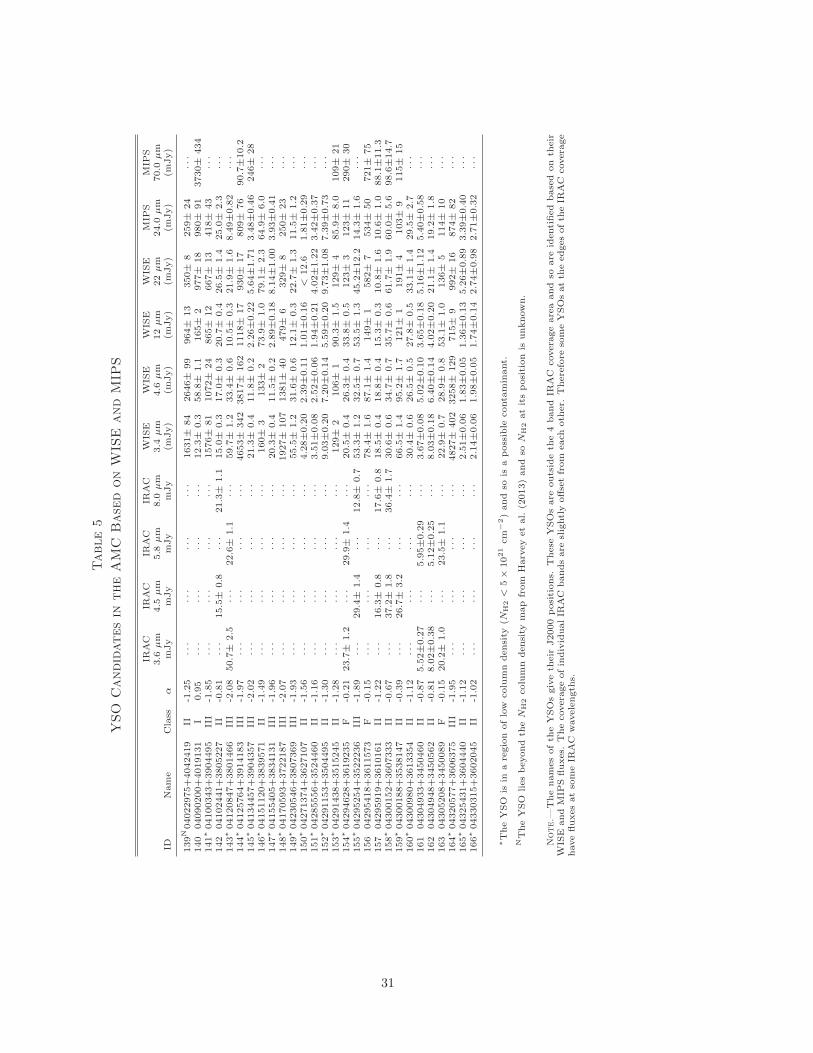
Table5

YSO

CandidatesintheAMC

Based

onW

ISE

and

MIPS

IRAC

IRAC

IRAC

IRAC

WIS

EW

ISE

WIS

EW

ISE

MIP

SM

IPS

3.6

μm

4.5

μm

5.8

μm

8.0

μm

3.4

μm

4.6

μm

12μm

22μm

24.0

μm

70.0

μm

IDName

Class

αmJy

mJy

mJy

mJy

(mJy)

(mJy)

(mJy)

(mJy)

(mJy)

(mJy)

139N04022975+4042419

II-1.25

···

···

···

···

1631±

84

2646±

99

964±

13

350±

8259±

24

···

140

04090200+4019131

I0.95

···

···

···

···

12.3±

0.3

58.8±

1.1

165±

2977±

18

980±

91

3730±

434

141∗04100343+3904495

III

-1.85

···

···

···

···

1576±

81

1072±

24

865±

12

667±

13

418±

43

···

142

04102441+3805227

II-0.81

···

15.5±

0.8

···

21.3±

1.1

15.0±

0.3

17.0±

0.3

20.7±

0.4

26.5±

1.4

25.0±

2.3

···

143∗04120847+3801466

III

-2.08

50.7±

2.5

···

22.6±

1.1

···

59.7±

1.2

33.4±

0.6

10.5±

0.3

21.9±

1.6

8.49±0.82

···

144∗04125764+3914183

III

-1.97

···

···

···

···

4653±

342

3817±

162

1118±

17

930±

17

809±

76

90.7±10.2

145∗04134457+3904357

III

-2.02

···

···

···

···

21.3±

0.4

11.8±

0.2

2.26±0.22

5.64±1.71

3.48±0.46

246±

28

146∗04151120+3839571

II-1.49

···

···

···

···

160±

3133±

273.9±

1.0

79.1±

2.3

64.9±

6.0

···

147∗04155405+3834131

III

-1.96

···

···

···

···

20.3±

0.4

11.5±

0.2

2.89±0.18

8.14±1.00

3.93±0.41

···

148∗04170593+3722187

III

-2.07

···

···

···

···

1927±

107

1381±

40

479±

6329±

8250±

23

···

149∗04230546+3807369

III

-1.93

···

···

···

···

55.5±

1.2

31.6±

0.6

12.1±

0.3

22.7±

1.3

11.5±

1.2

···

150∗04271374+3627107

II-1.56

···

···

···

···

4.28±0.20

2.39±0.11

1.01±0.16

<12.6

1.81±0.29

···

151∗04285556+3524460

II-1.16

···

···

···

···

3.51±0.08

2.52±0.06

1.94±0.21

4.02±1.22

3.42±0.37

···

152∗04291153+3504495

II-1.30

···

···

···

···

9.03±0.20

7.20±0.14

5.59±0.20

9.73±1.08

7.39±0.73

···

153∗04291438+3515245

II-1.28

···

···

···

···

129±

2106±

190.3±

1.5

129±

485.9±

8.0

109±

21

154∗04294628+3619235

F-0.21

23.7±

1.2

···

29.9±

1.4

···

20.5±

0.4

26.3±

0.4

33.8±

0.5

123±

3123±

11

290±

30

155∗04295254+3522236

III

-1.89

···

29.4±

1.4

···

12.8±

0.7

53.3±

1.2

32.5±

0.7

53.5±

1.3

45.2±12.2

14.3±

1.6

···

156

04295418+3611573

F-0.15

···

···

···

···

78.4±

1.6

87.1±

1.4

149±

1582±

7534±

50

721±

75

157

04295919+3610161

II-1.22

···

16.3±

0.8

···

17.6±

0.8

18.5±

0.4

18.8±

0.4

15.3±

0.3

10.8±

1.6

10.6±

1.0

88.1±11.3

158∗04300152+3607333

II-0.67

···

37.2±

1.8

···

36.4±

1.7

30.6±

0.6

34.7±

0.7

35.7±

0.6

61.7±

1.9

60.0±

5.6

98.6±14.7

159∗04300188+3538147

II-0.39

···

26.7±

3.2

···

···

66.5±

1.4

95.2±

1.7

121±

1191±

4103±

9115±

15

160∗04300980+3613354

II-1.12

···

···

···

···

30.4±

0.6

26.5±

0.5

27.8±

0.5

33.1±

1.4

29.5±

2.7

···

161

04304933+3450460

II-0.87

5.52±0.27

···

5.95±0.29

···

3.67±0.08

5.02±0.10

3.65±0.18

5.16±1.12

5.40±0.58

···

162

04304948+3450562

II-0.81

8.02±0.38

···

5.12±0.25

···

8.03±0.18

6.40±0.14

4.02±0.20

21.1±

1.4

19.2±

1.8

···

163

04305208+3450089

F-0.15

20.2±

1.0

···

23.5±

1.1

···

22.9±

0.7

28.9±

0.8

53.1±

1.0

136±

5114±

10

···

164∗04320577+3606375

III

-1.95

···

···

···

···

4827±

402

3258±

129

715±

9992±

16

874±

82

···

165∗04325431+3604440

II-1.12

···

···

···

···

2.51±0.06

1.83±0.05

1.36±0.13

5.26±0.89

3.39±0.40

···

166∗04330315+3602045

II-1.02

···

···

···

···

2.14±0.06

1.98±0.05

1.74±0.14

2.74±0.98

2.71±0.32

···

∗ TheYSO

isin

aregion

oflow

column

density

(NH2<

5×

1021cm

−2)and

sois

apossible

conta

minant.

NTheYSO

liesbeyond

theN

H2column

density

map

from

Harv

eyetal.

(2013)and

soN

H2atitsposition

isunknown.

Note.—

Thenamesofth

eYSOsgiveth

eir

J2000positions.

These

YSOsare

outsideth

e4band

IRAC

covera

geareaand

soare

identified

based

on

their

WIS

EandM

IPSfluxes.

Thecovera

geofindividualIR

AC

bandsare

slightlyoffsetfrom

each

oth

er.

Therefore

someYSOsatth

eedgesofth

eIR

AC

covera

ge

havefluxesatso

meIR

AC

wavelength

s.

31

Table 6

Relative ages

Region NYSO NI NF NII NI+F/NII

AMC 149 37 21 91 0.64OMC 3330 668 467 2195 0.52

Perseus 368 54 71 243 0.51Serpens 196 39 25 132 0.49

Ophiuchus 258 35 47 176 0.47IC 5146 128 29 12 87 0.47

Cepheus Flare 122 21 14 87 0.40Corona Australis 37 7 2 28 0.32

Lupus 95 8 12 75 0.27Chameleon II 22 2 1 19 0.16

References. — AMC: this work, OMC: Megeath et al. (2012),Perseus: Jørgensen et al. (2006), Serpens: Harvey et al. (2007),Ophiuchus: L. Allen, in preparation (see Evans et al. 2009), IC 5146:Harvey et al. (2008), Cepheus Flare: Kirk et al. (2009), Corona Aus-tralis: Peterson et al. (2011), Lupus: Merın et al. (2008), ChameleonII: Alcala et al. (2008)

32

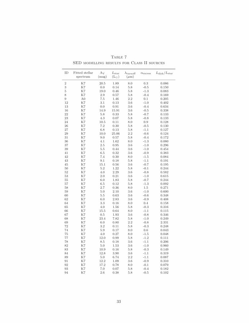
Table 7

SED modelling results for Class II sources

ID Fitted stellar AV Lstar λturnoff αexcess Ldisk/Lstar

spectrum (mag) (L�) (μm)

2 K7 20.5 1.89 8.0 0.3 0.0863 K7 0.0 0.14 5.8 -0.5 0.1505 K7 19.0 0.46 5.8 -1.3 0.0838 K7 2.9 0.57 5.8 -0.4 0.1699 A0 7.5 1.46 2.2 0.1 0.20512 K7 3.1 0.13 3.6 -1.0 0.40213 K7 0.0 0.91 3.6 -0.4 0.63416 K7 14.9 15.91 3.6 -0.5 0.33822 K7 5.8 0.33 5.8 -0.7 0.13323 K7 4.3 0.07 5.8 -0.8 0.13324 K7 10.5 0.11 8.0 0.9 0.12826 K7 7.2 0.30 5.8 -0.5 0.13027 K7 6.8 0.13 5.8 -1.1 0.12729 K7 10.0 25.06 2.2 -0.6 0.12431 K7 9.0 0.57 5.8 -0.4 0.17236 K7 4.1 1.62 8.0 -1.3 0.08037 K7 2.5 0.95 3.6 -1.0 0.29639 K7 5.5 0.44 3.6 -1.0 0.45441 K7 6.5 0.32 3.6 -0.9 0.38342 K7 7.4 0.30 8.0 -1.5 0.08443 K7 9.1 0.18 5.8 -1.1 0.19145 K7 15.1 0.56 3.6 -0.7 0.19550 K7 5.2 1.22 5.8 -0.1 0.24452 K7 4.0 2.29 3.6 -0.8 0.58253 K7 2.0 0.21 3.6 -1.0 0.61555 K7 6.0 1.83 5.8 -0.7 0.24457 K7 6.5 0.12 5.8 -1.3 0.09258 K7 2.7 0.36 8.0 1.5 0.27159 K7 5.0 2.10 3.6 -1.0 0.60060 K7 5.5 0.63 3.6 -0.6 0.34862 K7 6.0 2.83 3.6 -0.9 0.40864 K7 3.3 0.16 8.0 0.4 0.15865 K7 4.0 1.56 5.8 -0.3 0.31666 K7 15.5 0.64 8.0 -1.1 0.11567 K7 0.5 1.93 3.6 -0.8 0.34668 K7 23.4 7.82 5.8 -1.0 0.24969 K7 6.0 0.80 2.2 -0.8 2.33172 K7 3.2 0.11 5.8 -0.3 0.24874 K7 5.9 0.17 8.0 0.6 0.04375 K7 4.0 0.27 8.0 -1.5 0.04877 K7 12.0 0.99 5.8 -1.2 0.11178 K7 8.5 0.18 3.6 -1.1 0.20682 K7 5.0 1.53 3.6 -1.0 0.96083 K7 10.9 0.16 5.8 -0.3 0.14984 K7 12.8 3.90 3.6 -1.1 0.31989 K7 5.0 6.74 2.2 -1.1 0.08791 K7 12.2 1.09 3.6 -0.9 0.31092 K7 17.2 0.78 8.0 -0.1 0.07993 K7 7.0 0.07 5.8 -0.4 0.18294 K7 2.6 0.38 5.8 -0.5 0.102

33

Table 7—Continued

ID Fitted stellar AV Lstar λturnoff αexcess Ldisk/Lstar

spectrum (mag) (L�) (μm)

95 K7 0.5 0.08 3.6 -0.2 0.49996 K7 0.0 0.26 3.6 -0.6 0.43497 K7 4.0 0.80 3.6 -0.6 0.39498 K7 3.8 0.12 3.6 -0.6 0.32199 K7 7.0 0.53 5.8 -0.8 0.204102 K7 4.6 2.31 8.0 1.0 0.215104 K7 3.0 0.45 3.6 -0.6 0.319105 K7 4.8 0.13 8.0 -1.3 0.062106 K7 3.0 38.62 4.5 -0.1 0.110108 K7 10.2 0.11 8.0 2.4 1.830110 K7 1.5 0.83 3.6 -1.1 0.428113 K7 3.8 0.29 8.0 0.2 0.027114 K7 5.0 0.44 8.0 -1.0 0.053116 K7 1.0 0.24 3.6 -0.9 0.541119 K7 3.0 0.06 3.6 -0.8 0.241120 K7 9.4 0.55 5.8 -1.0 0.134122 K7 5.5 0.26 3.6 -0.5 1.164123 K7 23.0 0.76 8.0 -1.2 0.064127 K7 13.2 0.70 8.0 -1.1 0.059128 K7 2.0 3.04 2.2 -0.7 1.477129 K7 6.5 0.19 5.8 -0.8 0.096130 K7 4.5 0.14 8.0 -1.0 0.072132 K7 5.0 0.79 5.8 -0.1 0.599133 K7 4.0 0.31 8.0 0.7 0.040136 K7 0.0 0.15 5.8 -1.1 0.066137 K7 6.0 0.23 2.2 -1.8 1.156139 K7 15.9 52.81 2.2 -1.8 0.228142 K7 6.7 0.91 4.6 -0.9 0.112146 K7 0.0 5.13 4.6 -1.4 0.109150 K7 2.0 0.20 12.0 0.2 0.033151 K7 1.0 0.11 4.6 -0.8 0.123152 K7 2.6 0.48 4.6 -0.9 0.057153 K7 2.0 2.94 3.4 -1.1 0.349157 K7 6.4 0.98 4.6 -0.7 0.112158 K7 3.0 0.27 2.2 -0.7 1.353159 K7 1.0 0.17 2.2 -0.6 4.827160 K7 3.0 0.96 4.6 -0.9 0.215161 K7 10.0 0.21 3.6 -1.2 0.185162 K7 4.4 0.48 12.0 1.3 0.044165 K7 4.5 0.21 12.0 0.5 0.026166 K7 5.2 0.11 4.6 -0.9 0.095

34

Table 8

SED modelling results for Class III sources

ID Fitted stellar AV Lstar λturnoff αexcess Ldisk/Lstar

spectrum (mag) (L�) (μm)

11 A0 0.0 156.74 8.0 -1.6 0.01915 K7 1.5 0.79 24.0 · · · 0.01517 K7 20.0 0.40 8.0 -1.3 0.00619 K7 8.1 0.53 24.0 · · · 0.00954 K7 4.0 4.66 8.0 -1.0 0.01473 K7 4.3 0.30 8.0 -1.5 0.05380 K7 3.0 0.86 24.0 -99.0 0.008115 K7 2.6 0.78 8.0 0.1 0.041141 K7 6.0 137.96 12.0 -2.0 0.019143 K7 2.0 36.17 12.0 -0.8 0.009144 K7 4.8 326.26 12.0 -2.6 0.032145 K7 2.5 13.61 12.0 1.7 0.012147 K7 0.0 1.35 12.0 -0.0 0.007148 K7 6.0 191.61 24.0 -99.0 0.010149 K7 2.3 38.39 12.0 -0.7 0.007155 K7 0.0 2.92 8.0 -0.7 0.026164 K7 7.0 558.63 24.0 -99.0 0.003

Table 9

AMC Groups Summary

Group Position NYSO NII NF NI NI+F/NII Reff Rcirc Aspect Ratio Mean Surf. Dens.

(RA, Dec) (pc) (pc) (pc−2)

1a 67.562286, 35.239391 49 34 7 8 0.44 0.99 1.22 1.52 15.82 67.610970, 35.770126 23 12 7 4 0.92 0.55 1.23 5.01 24.13 67.671758, 35.541806 12 9 0 3 0.33 0.66 0.74 1.26 8.554 67.188288, 36.440921 10 4 1 5 1.5 0.48 0.69 2.03 13.35 67.708443, 34.958037 8 3 0 5 · · · · · · · · · · · · · · ·6 62.662345, 38.094258 6 5 0 1 · · · · · · · · · · · · · · ·7 62.525460, 40.037669 5 2 0 3 · · · · · · · · · · · · · · ·

aSeveral known members near LkHα 101 are missing in our YSO list, affecting the values reported for this group.

35