The regression discontinuity design in epidemiology · The regression discontinuity design in...

The regression discontinuity design inepidemiology

S.Geneletti1, G.Baio2 and A.P.Dawid3

1 London School of Economics and Political Science,2 University College London,3 University of Cambridge

30/11/2010

Outline

I What is the RD design?

I Causal inference

I RD design applied to statins

I THIN data

I Results

I Further work

What is the RD design?

I The regression discontinuity (RD) design was firstintroduced in the educational econometrics literature inthe 60’s [5]

I Recently other econometricians have become interested informal causal aspects [3, 6]

I The original idea was to exploit policy thresholds toestimate the causal effect of an educational intervention


ExampleI We want to know what the effect of going to college is on

income

I Comparing the income of individuals who attend collegeand those who do not will not tell us the effect of collegeattendance alone

I Confounders such as social class, ability, motivation etc.will make this difficult

I Classic problem of observational studies


Example cont’dI Often college scholarships are given on the basis of grades

obtained in final school examinations

I For example: if all exam grades are above 75% studentgets scholarship

I If one student gets 74% and another 76%

I Can we really consider them as coming from differentpopulations especially if in other respects (e.g. familyincome etc) they are the same?

I Given that there is natural variability in exam performanceeven for the same individual?


Public health ExampleI Many medicines are prescribed according to a particular

guidelineI Antiretroviral HIV drugs prescribed when patient’s CD4 counts

is less than 200 cells/mm3

I Blood pressure medication is prescribed when patient’s BP is140/90mmHg or above

I Statins are prescribed when e.g. 10 year Framingham riskscore is over 20%


Public Health Example cont’dI Consider the HIV patients.

I If one patient has a CD4 count of 195 and another of 205cells/mm3

I Theoretically, one patient gets the drugs while the otherdoesn’t

I If the two are the same in every other relevant respect

I Can we really consider them as coming from differentpopulations?

I Given that there is a natural variability in CD4 counts andin the instruments used to measure them?

RD design and confounding

Sharp DesignI The idea of the RD design is that the threshold behaves

like a randomising deviceI If we imagine that the thresholds are adhered to very

strictlyI termed sharp design

I Then we can think of the RD design as removing theconfounding due unobserved factors

I For education could be e.g. academic history, talent,motivation

I For HIV could also be unobserved health/personalcharacteristics

RD design and confounding

Fuzzy DesignI In public health contexts the sharp threshold is unlikely to

be adhered to

I Often GP’s override guidelines – generally because theyfeel patients will benefit from medication even when theydo not fit guidelines

I Often patients do not take the prescribed drugs asrecommended

I There are statistical methods that cater for these casesI termed fuzzy design

RD design and compliance

I For RD applied to GP prescription context there are twolayers of compliance

1. Compliance of GP to prescription guidelines [i.e. only givepatients with CD4 count below 200 cells/mm3 theantiretroviral drug]

2. Compliance of patient to prescription [i.e. take theantiretroviral drug twice a day every day]

I The RD design is related to compliance of the first type

I The RD’s relation to compliance means it is also relatedto intention-to-treat experiments

RD design and compliance

I RD with sharp threshold = randomised trial with perfectcompliance

I RD with fuzzy threshold = randomised trial with partialcompliance

I Mathematically the LHS and RHS of both equations areidentical

I So in the fuzzy design we don’t estimate an averagecausal effect but rather a complier causal effect

I The compliers are those who “respect” the threshold,

I For the GP prescription it is those who the GP prescribesthe drug to in accordance to the guidelines

I Whether the patients take the drugs as recommendedneeds to be dealt with separately

Causality in Statistics

MotivationI Causation = intervention

I However we cannot always intervene and randomise

I The trick is to understand what mechanisms behave inthe same way under intervention and under observation

I These mechanisms are then causal

Decision theoretic (DT) set-up

I F intervention variable, X other variables

I p(T = t|F = t,X) = 1 means set T = t e.g. byrandomisation in trial

I p(T |F = ∅, X) = p(T |X), T arises “naturally” in theobservational regime

I We estimate effects as predictive expectations (or otherfunctions) -i.e. we answer which treatment would benefita new unit exchangeable to those we have observed?

Simple problem first

I Consider theATE = E(Y |F = 1, T = 1)− E(Y |F = 0, T = 0)

I Where we leave out X for simplicity

I This is not necessarily the same as the “naive” treatmenteffectNTE = E(Y |F = ∅, T = 1)− E(Y |F = ∅, T = 0)

I Unless Y does not depend on how the treatment wasadministered

I I.e. F⊥⊥Y |T

Simple problem cont

F T Y

1. Y⊥⊥F |T means only the value of treatment matters for Y

2. However that does not tend to hold...

3. Usually there is a confounder U s.t.

U ⊥⊥ F

Y ⊥⊥ F |(U, T )

4. If U is unobserved and there is no randomisation thenATE 6= NTE

Simple problem cont

F T Y

U

1. Y⊥⊥F |T means only the value of treatment matters for Y

2. However that does not tend to hold...

3. Usually there is a confounder U s.t.

U ⊥⊥ F

Y ⊥⊥ F |(U, T )

4. If U is unobserved and there is no randomisation thenATE 6= NTE

Simple problem first

I If we look at adherence to the threshold as compliance

I We can introduce another variable binary Z – thethreshold indicator:

I If Z = 1 the individual is above the threshold

I If Z = 0 the individual is below the threshold

I When the threshold is strict then Z = F

RD design

F T Y

U

Z

I Z and F both have the same relationship with U ,T and Y

I This means Z can be used for causal inference

The RD design

AssumptionsA1 The threshold is set prior to the observed data and is not

changed after observationI Generally plausible as threshold set by the powers that be e.g.

gov’t agencies, NICE etc.

A2.1 Individuals close to the threshold are exchangeableI We have no reason to believe that the individuals just above

and below the threshold are differentI This is violated if individuals can change their outcome to fall

above or below the thresholdI Benefit fraud: individuals might say their income is below a

threshold in order to fall into a category that receives benefits

The RD design

Assumptions cont’dI Another way of expressing A2.1:

A2.1 The threshold is a randomising deviceI This means that a comparison of above and below gives us a

causal effect estimate of the treatment – at the thresholdI This is because randomisation is the gold standard for causal

inference as controls for confoundingI The question is how far above and how far below?

The RD design

The RD design

Assumptions cont’dA3 The assignment variable is continuous

I There cannot be a threshold w/out a continuous variableI Means we don’t have to worry about choosing bandsI We fit two separate regressions – one above and one below the

thresholdI Or assume a common slope and fit one regression – this

assumes effect is the same everywhere

The RD design

The causal effect

The continuous case: Sharp thresholdI Let Y be the outcome, W the assignment variable and T

the treatment indicator

I If the regressions are given by

E(Y )s = αs + βsW

where:I x is the value of X at the threshold;I s = b⇒W < w (below)I s = a⇒W ≥ w (above)

An estimate of the causal effect of the treatment is

ACE = E(Y |T = 1)− E(Y |T = 0)

= αb − αa + (βb − βa)w

I There are more sophisticated estimates[3, 6]

The causal effect

The continuous case: Fuzzy thresholdI Often there is not strict adherence to threshold

I Use the relationship between RD design and complianceto estimate the effect in this situation

I If Z = 1 if individual is above the threshold and Z = 0below then RD fuzzy estimate same as partial complianceestimate

I The local average treatment effect (LATE) – compliereffect [? ]

I Can be equated to fuzzy average causal effect (FACE)

LATE

The causal effect

The continuous case: Fuzzy thresholdI The formula for the fuzzy estimator is

FACE =E(Y |Z = 1)− E(Y |Z = 0)

E(T |Z = 1)− E(T |Z = 0)

I One estimate is:

αb − αa + (βb − βa)wˆp1|1 − ˆp1|0

I Where ˆpt|z is an estimate of p(T = t|Z = z)

I This is partly based on the compliance literature [1]

The RD design for binary outcomes

I Many outcomes in public health are binary (death, cvdevent)

I The RD design can be used for binary outcomes by usinglogistic regressions

I And then looking at treatment risk-ratios (RR)

I We don’t want to use odds ratios because we don’tnecessarily have rare outcomes

I Also, we want to be able to evaluate the RR at thethreshold

The RD design for binary outcomes

The causal risk ratio

The binary case: sharp thresholdI If we fit two separate logistic regressions

logit(p)s = αs + βsX,where s = {a, b} for above and below,

I then causal risk ratio at the threshold x is given by

RR =1 + exp(−{αb + βbx})1 + exp(−{αa + βax})

The causal risk ratio

The binary case: fuzzy thresholdI The fuzzy design for a binary outcome was originally

developed in the compliance literature by [2]

FRR =

1− p(Y |Z = 1)− p(Y |Z = 0)

p(Y |T = 1, Z = 1)p(T |Z = 1)− p(Y |T = 1, Z = 0)p(T |Z = 0)

I The different parts are estimated using logistic regressionsevaluated at the threshold

I The FRRI =RR when the design is sharpI Is further from the RR the more fuzzy the design

I This can also be derived along the same lines as the LATEbut much harder work!

The trouble with statins

I Statins are a class of drugs used to lower cholesterol andprescribed to prevent heart disease

I They are amongst the most prescribed drugs in the UK

I Some even suggest handing them out with fast food!


I Trials [7] show an average reduction of LDL cholesterol ofapproximately 2 mmol/l

I Also, NHS guidelines are to prescribe statins to individualsw/out previous CVD if their 10 year CVD score exceeds20% [4]

I CVD scores are predicted probabilities of event in next 10 yearsand are based on age, sex, smoking status, pressure, cholesteroland depending on type of score also diabetes, LVH etc.

I We could use the RD design with the threshold to seewhether the effect of statins is the same as in the trials


I In a second instance we can also try and determinewhether the prescription threshold is ideal

I By looking at CVD events and incorporating acost-effectiveness analysis

RD design design for statins

How do we measure the effects?I We have two outcomes of interest:

I Change in LDL cholesterol after treatmentI Occurrence of CVD events after treatment

I The threshold variable is the 10 year Framingham CVDscore

I Or another continuous variable that might be used by GPsto determine statin prescription

Example — RD design in the THIN data

I The THIN data set contains data from routine generalpractice prescriptions as well as information on thevariables that determine these prescriptions

I Individual characteristics (sex, date of birth, date ofregistration with practice, proxies of socioeconomic status)

I Medical history (GP visits, prescriptions, exams)

I This information can be used to characterise the patientswith respect to

I Measurements of health indicators that allow to estimate a riskof experiencing cardiovascular events

I Treatment with statinsI Measurements of suitable outcomes (e.g. LDL level, CHD

events, deaths)

Example (cont’d)

Preliminary analysis

I Data from THIN10 (a sub sample of 10 practices as ofFebruary 2009)

I Already existing “code lists” to identify and managecardiovascular events & related variables

I Identify relevant read codes & select records of patients withmeasurements for suitable variables

I Will need to update and perhaps modify this code list

I Created new (provisional) lists to identify records ofprescription for statin treatment

Example (cont’d)

I Estimated a cardiovascular risk predictorI Based on University of Edinburgh risk calculator

(http://cvrisk.mvm.ed.ac.uk/calculator/calc.asp)

Example (cont’d)

I Estimated a cardiovascular risk predictorI Combines two dimensions from Framingham risk calculatorI NB: Framingham risk calculator would be ideal, but it is not

consistently recorded in THINI Requires measurements of

I HLD and total cholesterol;I systolic blood pressure;I smoking and diabetes status and the presence of left

ventricular hypetrophy;I age and sex

I Problems with recording of smoking status, so will need tomake this estimation more robust

Example (cont’d)

Preliminary analysisI For the sake of simplicity we considered a simple

continuous outcomeI Measure of LDL cholesterol following the estimation of CVD

risk

I To simplify the analysis, we grouped the patientsaccording to their age at the risk prediction

I Bins of 5 years (50-54 — 85+)

I Each patient was associated with the treatment group ifthey had a prescription for statins in the year following therisk prediction

Example — Sharp design

I Assume that the design is sharp (i.e. “perfect” treatmentallocation)

I Run two regression analysesI Control for sex, risk and age at LDL measurement

I Treatment effect measured as ACE

ACE = E(Y |T = 1)− E(Y |T = 0)


0.0 0.1 0.2 0.3

02

46

Age at prediction = 50−54 (n = 1484) ACE = −0.271

Predicted risk score

LDL

(mm

ol/l)

Not TreatedTreated

0.0 0.1 0.2 0.3 0.4 0.5 0.6

01

23

45

67



LDL

(mm

ol/l)

Not TreatedTreated

0.0 0.1 0.2 0.3 0.4 0.5 0.6

12

34

56



LDL

(mm

ol/l)

Not TreatedTreated

0.0 0.2 0.4 0.6

02

46

8



LDL

(mm

ol/l)

Not TreatedTreated

0.0 0.2 0.4 0.6 0.8

24

68

Age at prediction = 70−74 (n = 2142) ACE = 0.0552


LDL

(mm

ol/l)

Not TreatedTreated

0.0 0.2 0.4 0.6 0.8 1.0

12

34

56

7



LDL

(mm

ol/l)

Not TreatedTreated

0.0 0.2 0.4 0.6 0.8 1.0

12

34

5



LDL

(mm

ol/l)

Not TreatedTreated

0.0 0.1 0.2 0.3 0.4 0.5 0.6 0.7

12

34

5

Age at prediction = 85+ (n = 251) ACE = 3.32


LDL

(mm

ol/l)

Not TreatedTreated


I ACE reasonably stable and negative (i.e. treatmentdecreases level of LDL) for age groups 50-54 up to 70-74

I Older age groups show very unstable estimates (few datapoints in the treatment group!)

I Overall, treatment effect is small


0.0 0.2 0.4 0.6

02

46

8



LDL

(mm

ol/l)

Not TreatedTreated


I ACE reasonably stable and negative (i.e. treatmentdecreases level of LDL) for age groups 50-54 up to 70-74

I Older age groups show very unstable estimates (few datapoints in the treatment group!)

I Overall, treatment effect is small

I More importantly, the design is not sharp!

Example — Fuzzy design

0.1 0.2 0.3

02

46

Age at prediction = 50−54 (n = 1484)


LDL

(mm

ol/l)

Not TreatedTreated

0.0 0.1 0.2 0.3 0.4 0.5

01

23

45

67



LDL

(mm

ol/l)

Not TreatedTreated

0.0 0.1 0.2 0.3 0.4 0.5 0.6

24

68

10



LDL

(mm

ol/l)

Not TreatedTreated

0.1 0.2 0.3 0.4 0.5 0.6

02

46

8


Predicted risk scoreLD

L (m

mol

/l)

Not TreatedTreated

0.0 0.2 0.4 0.6 0.8

24

68



LDL

(mm

ol/l)

Not TreatedTreated

Example — Fuzzy design

I Under these circumstances, we cannot use ACE toestimate the causal effect, but need to build FACE

I For this preliminary analysis, we estimate the denominatorusing the observed raw proportions

I There are a few possible ways of computing the estimandI By threshold onlyI By treatment onlyI By treatment & threshold

Example (cont’d)

0.1 0.2 0.3

02

46

Age at prediction = 50−54 (n = 1484) FACE = −0.326


LDL

(mm

ol/l)

Not TreatedTreated

0.0 0.1 0.2 0.3 0.4 0.5

01

23

45

67



LDL

(mm

ol/l)

Not TreatedTreated

0.0 0.1 0.2 0.3 0.4 0.5 0.6

24

68

10



LDL

(mm

ol/l)

Not TreatedTreated

0.1 0.2 0.3 0.4 0.5 0.6

02

46

8



LDL

(mm

ol/l)

Not TreatedTreated

Some results

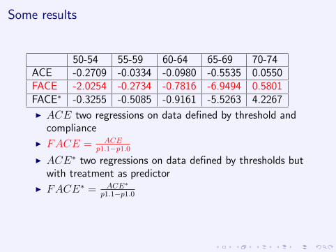
50-54 55-59 60-64 65-69 70-74ACE -0.2709 -0.0334 -0.0980 -0.5535 0.0550FACE -2.0254 -0.2734 -0.7816 -6.9494 0.5801FACE∗ -0.3255 -0.5085 -0.9161 -5.5263 4.2267

I ACE two regressions on data defined by threshold andcompliance

I FACE = ACEp1.1−p1.0

I ACE∗ two regressions on data defined by thresholds butwith treatment as predictor

I FACE∗ = ACE∗

p1.1−p1.0

Some results

I Estimates of FACE are very unstable

I Need to come up with more robust estimates ofdenominator

Example — Comments

I The results are only indicative of the underlying causalmechanism, due to a series of factors

I Data need to be made more robust (include more practices &more precise information on crucial predictor, such as smokingstatus)

I Account properly for the two layers on “non compliance”I GPs prescribing below threshold (or not prescribing above)I Individual compliance (patients prescribed statins who do not

take them continuously)

I There seems to be an effect of treatment, especially insome age groups, but more analyses are required

I Careful stratification by sexI Control for more health conditions

Where to next?

I Clean up data more and apply to whole THIN dataset

I Find more stable/robust estimates of the denominator ofthe FACE

I Incorporate cost-effectiveness analysis

I Apply RD design to other drugs/screening

References

[1] A. P. Dawid. Causal inference using influence diagrams: The problem of partial compliance (with Discussion).In P.J. Green, N.L. Hjort, and S. Richardson, editors, Highly Structured Stochastic Systems, pages 45–81.Oxford University Press, 2003.

[2] MA Hernan and JM Robins. Instruments for causal inference - An epidemiologist’s dream? Epidemiology,17(4):360–372, JUL 2006.

[3] Guido W. Imbens and Thomas Lemieux. Regression discontinuity designs: A guide to practice. Journal ofEconometrics, 142(2):615 – 635, 2008. The regression discontinuity design: Theory and applications.

[4] NICE. Quick reference guide: Statins for the prevention of cardiovascular events, 2008.

[5] DL. Thistlethwaite and DT. Campbell. Regression-Discontinuity Analysis - An alternative to the ex-post-factoexperiment. Journal of Educational Psychology, 51(6):309–317, 1960.

[6] G. van der Klaauw. Regression-discontinuity analysis: A survey of recent developments in economics. Labour,22(2):219–245, 2008.

[7] S. Ward, L. Jones, A. Pandor, M. Holmes, R. Ara, A. Ryan, W. Yeo, and N. Payne. A systematic review andeconomic evaluation of statins for the prevention of coronary events. Health Technology Assessment, 11(14),2007.

Deriving the LATE

I Pretend we’re looking at a randomised trial with partialcompliance

I Introduce three variablesI Z the randomised treatment – not necessarily complied toI U the unobserved confoundersI CZ the preferred treatment under Z

Deriving the LATE

Z T Y

U

I If the DAG above describes the situation

I Then we can replace U with CZ

Deriving the LATE

Z T Y

CZ

I If the DAG above describes the situation

I Then we can replace U with CZ

Deriving the LATE

I The CZ ’s look a bit like counterfactuals

I But they aren’t as they represent preferences that you canelicit prior to any treatment being assigned

I So they are random variablesI We assume that T = CZ ,

I i.e. the treatment actually taken is the preferred treatment

I We also assume monotonicityI Individuals do not want to do the opposite of what they are

recommendedI p(C0 = 1, C1 = 0) = 0

Deriving the LATE

I By using this set-up it is possible to derive an estimate ofthe LATE

I based on only the Z’s and the T ’sI rather than the CZ ’s which we cannot directly observe

back

The regression discontinuity design in epidemiology · The regression discontinuity design in...

Documents

Transcript of The regression discontinuity design in epidemiology · The regression discontinuity design in...