Regression

Discontinuity MethodDay 3, Lecture 2

By Ragui Assaad

Training on Applied Micro-Econometrics and Public Policy Evaluation

July 25-27, 2016

Economic Research Forum

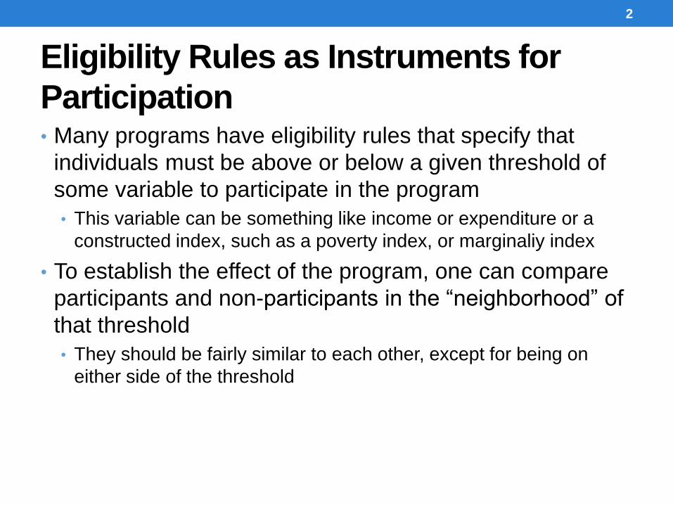
Eligibility Rules as Instruments for

Participation• Many programs have eligibility rules that specify that

individuals must be above or below a given threshold of

some variable to participate in the program

• This variable can be something like income or expenditure or a

constructed index, such as a poverty index, or marginaliy index

• To establish the effect of the program, one can compare

participants and non-participants in the “neighborhood” of

that threshold

• They should be fairly similar to each other, except for being on

either side of the threshold

2

Sharp vs. Fuzzy Regression

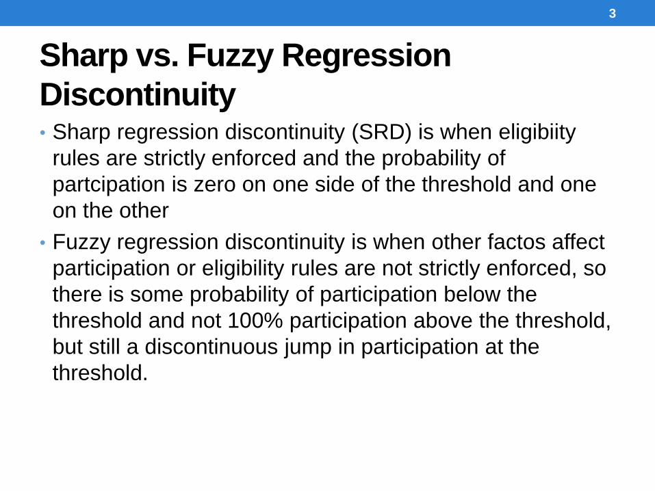
Discontinuity• Sharp regression discontinuity (SRD) is when eligibiity

rules are strictly enforced and the probability of

partcipation is zero on one side of the threshold and one

on the other

• Fuzzy regression discontinuity is when other factos affect

participation or eligibility rules are not strictly enforced, so

there is some probability of participation below the

threshold and not 100% participation above the threshold,

but still a discontinuous jump in participation at the

threshold.

3

SRD vs FRD

4

RD and IV Approaches: what is the

connection?• RD approach introduces introduces an exogenous

variable (a dummy for being below or above the

threshold) that strongly affects participation but that does

not directly affect the outcome of interest, conditional on

controlling for the continuous effects of the eligibility

variable itself.

• This variable can essentially serve as an IV for

participation

5

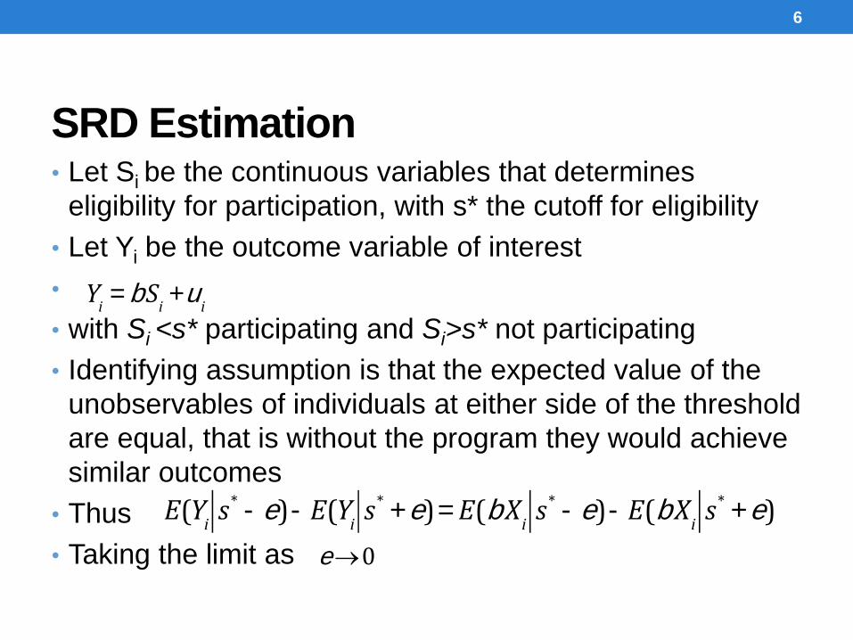
SRD Estimation• Let Si be the continuous variables that determines

eligibility for participation, with s* the cutoff for eligibility

• Let Yi be the outcome variable of interest

•

• with Si <s* participating and Si>s* not participating

• Identifying assumption is that the expected value of the

unobservables of individuals at either side of the threshold

are equal, that is without the program they would achieve

similar outcomes

• Thus

• Taking the limit as

6

Y

i= bS

i+u

i

E(Y

is* -e)- E(Y

is* +e)= E(bX

is* -e)- E(bX

is* +e)

e®0

7

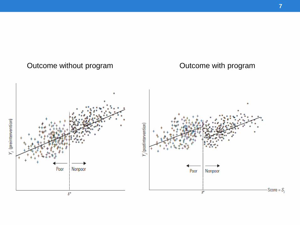
Outcome without program Outcome with program

SRD Estimation

8

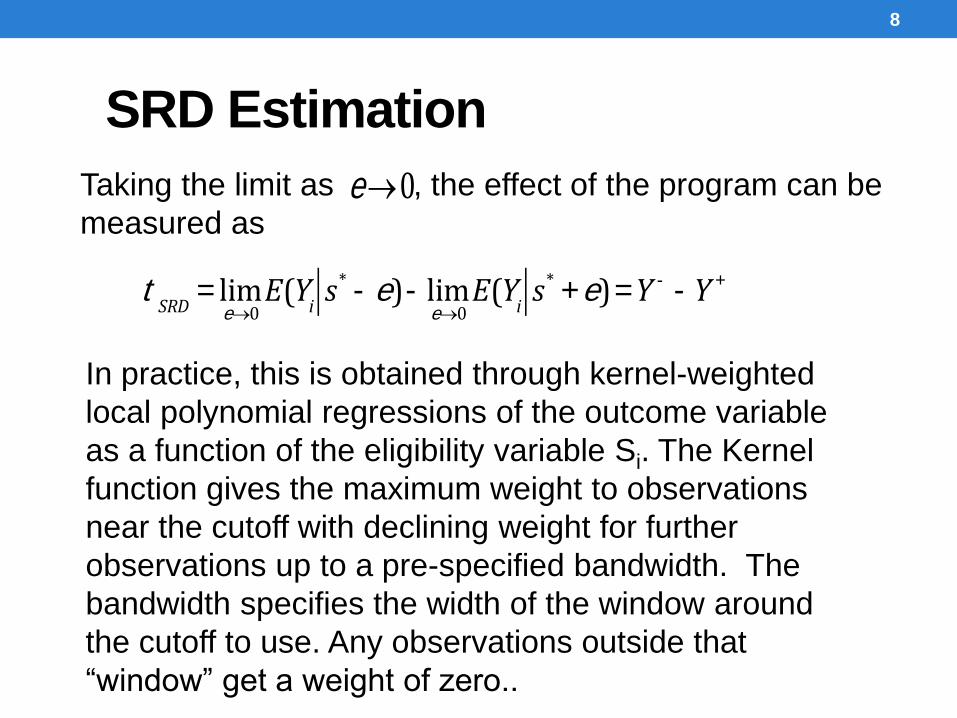
e®0Taking the limit as , the effect of the program can be

measured as

t

SRD= lim

e®0E(Y

is* -e)- lim

e®0E(Y

is* +e)=Y - -Y +

In practice, this is obtained through kernel-weighted

local polynomial regressions of the outcome variable

as a function of the eligibility variable Si. The Kernel

function gives the maximum weight to observations

near the cutoff with declining weight for further

observations up to a pre-specified bandwidth. The

bandwidth specifies the width of the window around

the cutoff to use. Any observations outside that

“window” get a weight of zero..

SRD Estimations

• Use these regressions to estimate the mean outcome

below and above the threshold in a narrow window

around the threshold

• Use these means to construct the test statistic

• Use bootstrapping to calculate SE’s

9

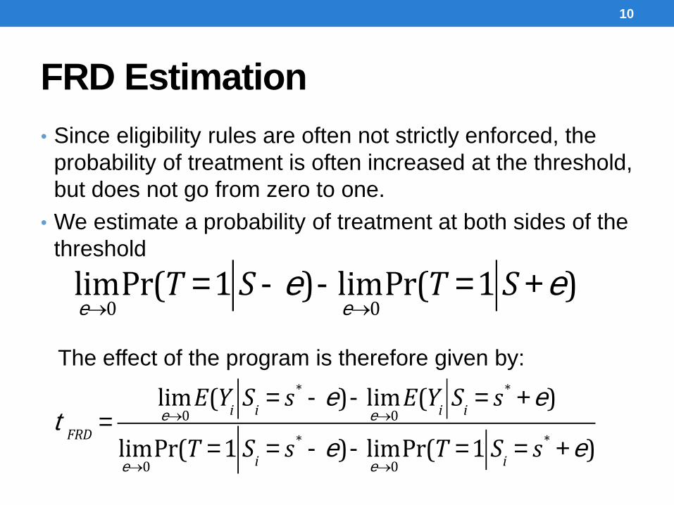
FRD Estimation

• Since eligibility rules are often not strictly enforced, the

probability of treatment is often increased at the threshold,

but does not go from zero to one.

• We estimate a probability of treatment at both sides of the

threshold

10

lime®0

Pr(T =1 S -e)-lime®0

Pr(T =1 S +e)

The effect of the program is therefore given by:

tFRD

=lime®0

E(Yi

Si= s* -e )- lim

e®0E(Y

iS

i= s* +e)

lime®0

Pr(T = 1 Si= s* -e )- lim

e®0Pr(T =1 S

i= s* +e)

FRD Estimation in Practice

• Again we use kernel-weighted local polynomial regression to estimate the outcome as a function of the eligibility variable Si

at each side of the threshold for the numerator of the ratio

• We then estimate a kernel-weighted local polynomial regression of the treatment variable as a function of the eligibility variable Si at each side of the threshold for the denominator.

• Use the outcome regressions to estimate the mean outcomes below and above the threshold in a window around the threshold

• Use the treatment probability regressions to estimate the mean probabilities of treatment below and above the threshold

• Construct the test-statistic

• Use bootstrapping to obtain SE’s

11

Sensitivity Analysis

• Results are likely to depend on the width of the window

around the threshold

• Conduct sensitivity analysis around the bandwidth of the

kernel function and the width of the window used to

calculate the mean outcomes and mean probability of

treatment

12

Case Study: The Impact of a

Community Development and

Poverty Reduction Program in

Morocco

Caroline Krafft

Joint work with Safaa El-Kogali, Touhami Abdelkhalek, Mohamed Benkassmi, Monica Chavez, Lucy Bassett and Fouzia Ejjanoui

13

Background: INDH

• To combat poverty and inequality, in 2005 Morocco

launched the National Human Development Initiative

(INDH)

• Community driven development program

• First phase: 2005-2010

• US$1.7 billion of spending, 700 local plans, 22,000

activities, 5.2 million beneficiaries

• In rural areas, targeted communes with high poverty rates

• Additional communes targeted in 2011-2015 (second

phase of US$2.1 billion)

14

Data for Evaluating INDH

15

• Decision to evaluate INDH occurred after program rolled out

• No data from before the program

• In rural areas, communities were targeted if poverty (map) rates were 30% or higher

• Targeting allows for regression discontinuity design (RDD)

• National Human Development Observatory (ONDH) INDH impact evaluation panel survey

• Panel survey on the household level• Communes just above and below cutoff (27-32%)

• 12 households per commune, 124 rural communes

• Rounds in 2008, 2011, 2013 (71% of control in Phase II)

Outcomes

16

• Economic outcomes

• Income

• Consumption

• Assets

• All in 2013 dirham, annually, and per capita

• US$1=8.17 Moroccan dirham

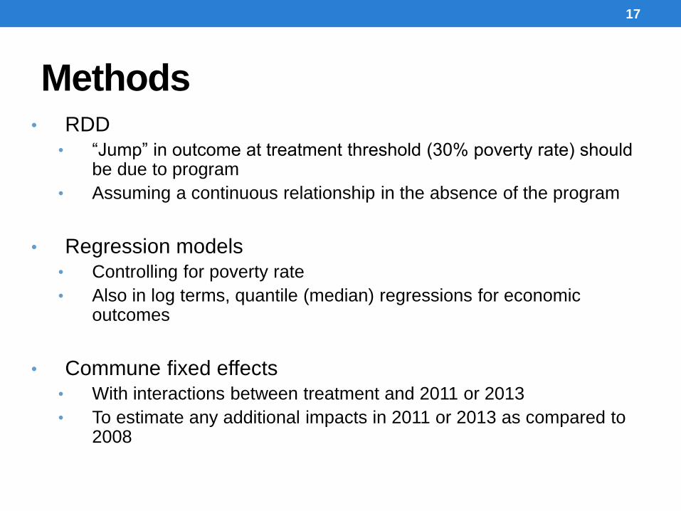
Methods

17

• RDD

• “Jump” in outcome at treatment threshold (30% poverty rate) should be due to program

• Assuming a continuous relationship in the absence of the program

• Regression models

• Controlling for poverty rate

• Also in log terms, quantile (median) regressions for economic outcomes

• Commune fixed effects

• With interactions between treatment and 2011 or 2013

• To estimate any additional impacts in 2011 or 2013 as compared to 2008

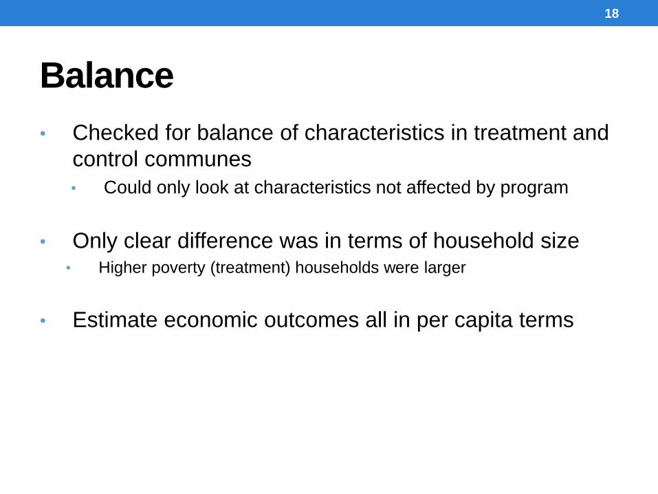
Balance

18

• Checked for balance of characteristics in treatment and

control communes

• Could only look at characteristics not affected by program

• Only clear difference was in terms of household size• Higher poverty (treatment) households were larger

• Estimate economic outcomes all in per capita terms

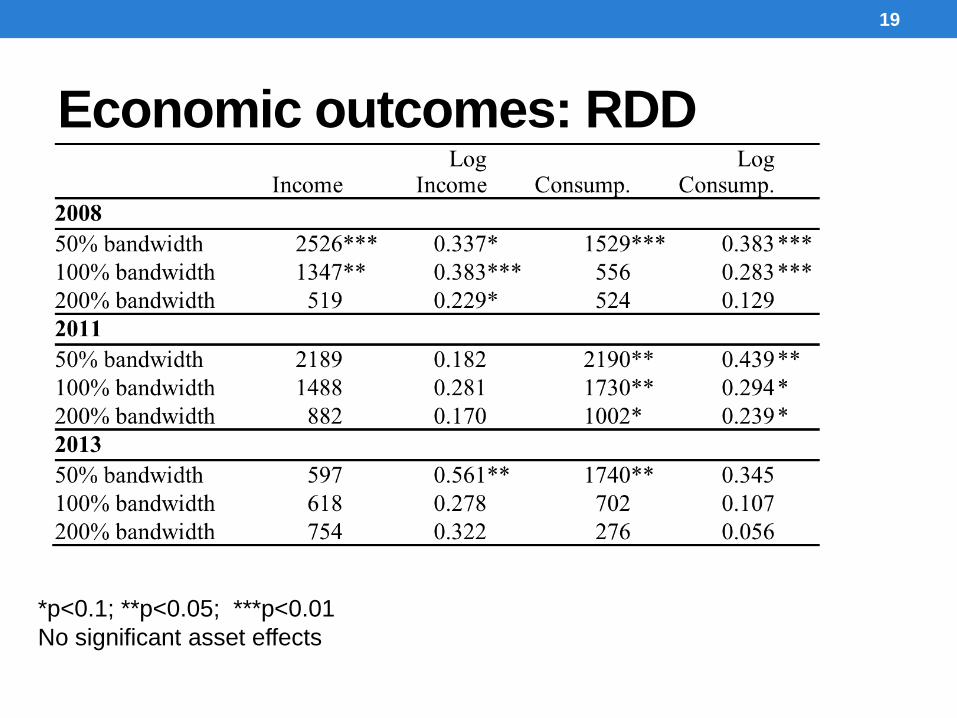
Economic outcomes: RDD

19

*p<0.1; **p<0.05; ***p<0.01

No significant asset effects

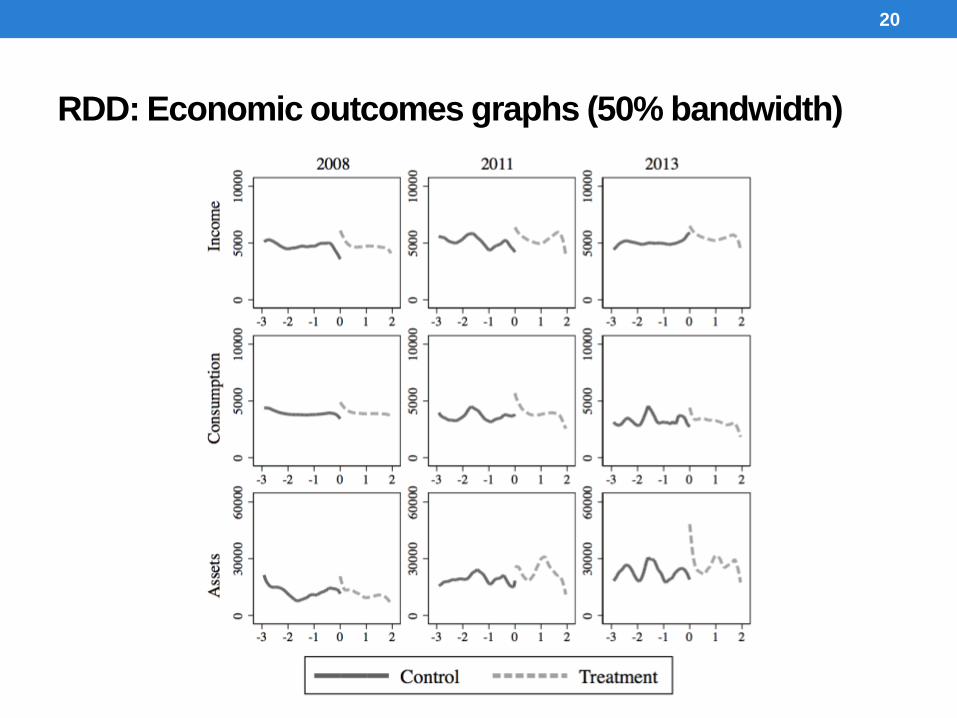
RDD: Economic outcomes graphs (50% bandwidth)

20

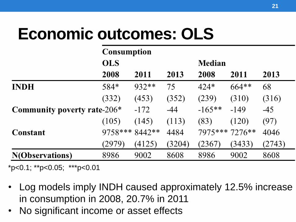
Economic outcomes: OLS

21

*p<0.1; **p<0.05; ***p<0.01

• Log models imply INDH caused approximately 12.5% increase

in consumption in 2008, 20.7% in 2011

• No significant income or asset effects

Limitations

22

• No baseline data from before the program• Treatment not randomly assigned

• RDD method• If communities are similar right around cutoff, as good as random

• Extremely sensitive to bandwidth

• Program expanded to control areas in 2011 onwards

• Generalizability• Just around cutoff for inclusion

• Problems in implementing INDH, particularly coordination challenges