HCEO WORKING PAPER SERIES

Working Paper

The University of Chicago1126 E. 59th Street Box 107

Chicago IL 60637

www.hceconomics.org

Breaking Ties:

Regression Discontinuity Design Meets Market Design

ú

Atila Abdulkadiro�lu Joshua D. Angrist Yusuke Narita Parag A. Pathak

†

March 6, 2019

Abstract

Centralized school assignment algorithms must distinguish between applicants with thesame preferences and priorities. This is done with randomly assigned lottery numbers, non-lottery tie-breakers like test scores, or both. The New York City public high school matchillustrates the latter, using test scores, grades, and interviews to rank applicants to screenedschools, combined with lottery tie-breaking at unscreened schools. We show how to identifycausal e�ects of school attendance in such settings. Our approach generalizes regressiondiscontinuity designs to allow for multiple treatments and multiple running variables, someof which are randomly assigned. Lotteries generate assignment risk at screened as wellas unscreened schools. Centralized assignment also identifies screened school e�ects awayfrom screened school cuto�s. These features of centralized assignment are used to assess thepredictive value of New York City’s school report cards. Grade A schools improve SAT mathscores and increase the likelihood of graduating, though by less than OLS estimates suggest.Selection bias in OLS estimates is egregious for Grade A screened schools.

úThis paper is a revision of our NBER Working Paper 24172, “Impact Evaluation in Matching Markets withGeneral Tie-Breaking.” We thank Nadiya Chadha, Andrew McClintock, Sonali Murarka, Lianna Wright, andthe sta� of the New York City Department of Education for answering our questions and facilitating accessto data. Don Andrews, Tim Armstrong, Eduardo Azevedo, Yeon-Koo Che, Glenn Ellison, Brigham Frandsen,John Friedman, Justine Hastings, Guido Imbens, Jacob Leshno, Whitney Newey, Ariel Pakes, Pedro Sant’Anna,Hal Varian and seminar participants at Columbia, Montreal, Harvard, Hebrew University, Google, the NBERSummer Institute, the NBER Market Design Working Group, the FRB of Minneapolis, CUNY, Yale, Hitotsubashi,and Tokyo provided helpful feedback. We’re especially indebted to Adrian Blattner, Ignacio Rodriguez, andSuhas Vijaykumar for expert research assistance and to MIT SEII program manager Eryn Heying for invaluableadministrative support. We gratefully acknowledge funding from the Laura and John Arnold Foundation, theNational Science Foundation (under awards SES-1056325 and SES-1426541), and the W.T. Grant Foundation.Abdulkadiro�lu is a Scientific Advisory Board members of the Institute for Innovation in Public School Choice.Angrist’s daughter teaches at a Boston charter school.

†Abdulkadiro�lu: Department of Economics, Duke University and NBER, email: atila.abdulkadiroglu@duke.edu.Angrist: Department of Economics, MIT and NBER, email: angrist@mit.edu. Narita: Department of Economicsand Cowles Foundation, Yale University, email: yusuke.narita@yale.edu. Pathak: Department of Economics, MITand NBER, email: ppathak@mit.edu.

1 Introduction

Large urban school districts increasingly use sophisticated matching mechanisms to assign theirseats. In addition to producing fair and transparent admissions decisions, centralized assignmentschemes o�er a unique resource for research and accountability: the data they generate canbe used to construct unbiased estimates of school value-added. This research dividend arisesfrom the tie-breaking embedded in centralized matching. A commonly used school matchingscheme, deferred acceptance (DA), takes as input information on applicant preferences andschool priorities. In settings where slots are scarce, tie-breaking variables distinguish betweenapplicants who have the same preferences and are subject to the same priorities. Holdingpreferences and priorities fixed, stochastic tie-breakers become a source of quasi-experimentalvariation in school assignment.

Many districts break ties with a single random variable, often described as a “lottery num-ber”. Abdulkadiro�lu, Angrist, Narita and Pathak (2017b) show that lottery tie-breaking assignsstudents to schools as in a stratified randomized trial. That is, conditional on preferences andpriorities, admission o�ers generated by such systems are randomly assigned and therefore in-dependent of potential outcomes. In practice, however, preferences and priorities, which we callapplicant type, are too finely distributed for full non-parametric conditioning to be useful. Thekey to a feasible DA-based research design is the DA propensity score, defined as the proba-bility of school assignment conditional on preferences and priorities. In a match with lotterytie-breaking, conditioning on the scalar DA propensity score is su�cient to make assignmentignorable, that is, independent of potential outcomes. Moreover, because the DA propensityscore for a market with lottery tie-breaking depends on only a few school-level cuto�s, the scoredistribution is much coarser than the distribution of types.

We turn here to the problem of crafting research designs from a broad class of assignmentmechanisms in which the tie-breaking variable is non-random and potentially correlated withunobserved potential outcomes. Non-random tie-breaking, used for school assignment in Boston,Chicago, and New York City, raises important challenges for causal inference in matching mar-kets.1 Most importantly, seat assignment under non-random tie-breaking is no longer ignorableconditional on type. Exam schools, for instance, select students with higher test scores, and thesehigh-scoring students can be expected to do well no matter where they go to school. In regres-sion discontinuity (RD) parlance, the running variable used to distinguish between applicantsof the same type is a source of omitted variables bias (OVB).

Other barriers to causal inference in this setting are raised by the fact that the propensityscore in a general tie-breaking scenario depends on the unknown distribution of tie-breakers for

1Non-lottery tie-breaking embedded in centralized assignment schemes has been used in econometric researchon schools in Chile (Hastings, Neilson and Zimmerman, 2013; Zimmerman, 2019), Ghana (Ajayi, 2014), Italy(Fort, Ichino and Zanella, 2016), Kenya (Lucas and Mbiti, 2014), Norway (Kirkeboen, Leuven and Mogstad, 2016),Romania (Pop-Eleches and Urquiola, 2013), Trinidad and Tobago (Jackson, 2010, 2012; Beuermann, Jackson andSierra, 2016), and the U.S. (Abdulkadiro�lu, Angrist and Pathak, 2014; Dobbie and Fryer, 2014; Barrow, Sartainand de la Torre, 2016). These studies treat di�erent schools and tie-breakers in isolation, without exploitingcentralized assignment. Other related work considers estimation methods in regression discontinuity designs withmultiple assignment variables and multiple cuto�s (Papay, Willett and Murnane, 2011; Zajonc, 2012; Wong,Steiner and Cook, 2013; Cattaneo, Titiunik, Vazquez-Bare and Keele, 2016).

each applicant type. This means that the propensity score under general tie-breaking may beno coarser than the underlying type distribution. Moreover, with an unknown distribution oftie-breakers, we cannot easily estimate the propensity score by simulation. These problems aresolved here by integrating the non-parametric RD framework introduced by Hahn, Todd andVan der Klaauw (2001) with the large-market matching model used to study random tie-breakingin Abdulkadiro�lu et al. (2017b).2 Our results provide an easily-implemented framework for awide variety of assignment schemes with multiple cuto�s and multiple running variables, someof which may be randomly assigned.3

The research value of a matching market with general tie-breaking is demonstrated throughan investigation of the predictive value of New York City (NYC) high school report cards.Specifically, we exploit variation generated by the NYC high school match, which uses a DAmechanism that integrates distinct non-lottery “screened school” tie-breaking with a commonlottery tie-breaker at “unscreened schools". The quasi-experimental assignment variation gen-erated by this system is used here to answer questions about school quality in a two-stage leastsquares (2SLS) setup.

Our results show that attendance at one of NYC’s “Grade A schools” boosts SAT mathscores modestly and may have a small e�ect on high school graduation. These e�ects aresmaller than the corresponding ordinary least squares (OLS) estimates of Grade A value-added.Grade A attendance also boosts measures of college and career readiness. The practical util-ity of our approach is seen in the markedly increased precision of estimates that exploit allsources of assignment risk. Motivated by the ongoing debate over screened admissions policiesin public schools, we also compare 2SLS estimates of Grade A e�ects computed separately forscreened and unscreened schools. These are similar, but OLS estimates showing a large GradeA screened school advantage are especially misleading. Finally, we address concerns that RDe�ects identified solely for applicants close to screened school cuto�s might be idiosyncratic.Specifically, we show that centralized assignment identifies screened school e�ects for applicantswith tie-breakers away from screened school cuto�s.

2 School Choice Experiments

School assignment problems are defined by a set of applicants, schools, and school capacities.Applicants have preferences over schools while schools have priorities over applicants. For ex-ample, schools may prioritize applicants who live nearby or with currently enrolled siblings. Lets = 0, 1, ..., S index schools, where s = 0 represents an outside option. The letter I denotes a setof applicants, indexed by i. I may be finite or, in our large-market model, a continuum, withapplicants indexed by values in the unit interval. Seating is constrained by a capacity vector,q = (q0, q1, q2, ..., qS), where q

s

is defined as the proportion of I that can be seated at school s.We assume q0 = 1.

2We also build upon the “local random assignment” interpretation of nonparametric RD, discussed by Frölich(2007); Cattaneo, Frandsen and Titiunik (2015); Cattaneo, Titiunik and Vazquez-Bare (2017); Frandsen (2017)and Sekhon and Titiunik (2017). See Lee and Lemieux (2010) for a survey of RD methods.

3Large-market results for the special case of serial dictatorship with a single non-random tie-breaker aresketched in Abdulkadiro�lu, Angrist, Narita, Pathak, and Zarate (2017a).

2

Applicant i’s preferences over schools constitute a partial ordering, �i

, where a �i

b meansthat i prefers school a to school b. Each applicant is also granted a priority at every school.Let ⇢

is

2 {1, ...,K,1} denote applicant i’s priority at school s, where ⇢is

< ⇢

js

means schools prioritizes i over j. For instance, ⇢

is

= 1 might encode the fact that applicant i has siblingpriority at school s, while ⇢

is

= 2 encodes neighborhood priority, and ⇢

is

= 3 for everyone else.We use ⇢

is

= 1 to indicate that i is ineligible for school s. Many applicants share priorities ata given school, in which case ⇢

is

= ⇢

js

for some i 6= j. The vector ⇢i

= (⇢

i1, ..., ⇢iS) recordsapplicant i’s priorities at each school.

Applicant type is defined as ✓i

= (�i

, ⇢

i

), that is, the combination of an applicant’s preferencesand priorities at all schools. We say that an applicant of type ✓ has preferences �

✓

and priorities⇢

✓

. ⇥ denotes the set of possible types. A mechanism is a rule determining assignment as afunction of type and a set of tie-breaking variables that schools use to discriminate betweenapplicants of the same type.

In our framework, tie-breakers and priorities are distinct because the latter are fixed, whilethe former are modeled as random variables. Resampling tie-breakers makes the mechanismsof interest to us stochastic: the assignment distribution generated by any stochastic mechanismis induced by the distribution of tie-breakers. In particular, stochastic mechanisms generate aprobability or “risk” of assignment for each applicant to each school. Assignment risk is createdby repeatedly drawing tie-breakers from each applicant’s tie-breaker distribution and re-runningthe match, fixing other market features.

Tie-breakers may be uniformly distributed lottery numbers, in which case they’re distributedindependently of type, or variables like entrance exam scores, that depend on type. With lotterytie-breaking, the relevant distribution is a permutation distribution under which all applicantorderings are equally likely. Tie-breakers overlap with the concept of a running variable insimple RD-style research designs. We prefer the term “tie-breaker” because this highlights therole such variables play in a centralized match. As is typical of RD, non-lottery tie-breakers inschool choice are not uniformly distributed, and may depend on applicant characteristics likerace or potential outcomes, as well as on type.

To describe assignment risk more formally, consider first a market with a single continuouslydistributed tie-breaker common to all schools, denoted R

i

for applicant i. Although R

i

is notnecessarily uniform, we assume that it’s scaled (preserving position or rank) to be distributedover [0, 1], with continuously di�erentiable cumulative distribution function F

i

R

(an assumptionwe maintain throughout). These common support and smoothness assumptions notwithstand-ing, tie-breakers may be correlated with type, so that R

i

and R

j

for applicants i and j are notnecessarily identically or uniformly distributed, though they’re assumed to be independent ofone another.4

By the law of iterated expectations, the probability type ✓ applicants have a tie-breakerbelow any value r is F

R

(r|✓) ⌘ E[F

i

R

(r)|✓i

= ✓], where F

i

R

(r) is F

i

R

evaluated at r and theexpectation is assumed to exist. To be concrete, suppose that the tie-breaker is a test score.

4We assume that sets of applicants of the form {i|a < Ri

b}, where a and b are constants, are measurable.A su�cient condition for this is that the mapping from i 2 [0, 1] to R

i

2 [0, 1] be left continuous (Aliprantis andBorder, 2006). This is satisfied by reordering applicants by their tie-breaker realizations.

3

Suppose also that type ✓0 applicants do exceptionally well on tests and therefore have tie-breakervalues drawn from a distribution with higher mean than the score distribution for type ✓1. Thisimplies F

R

(r|✓0) 6= F

R

(r|✓1). By contrast, when R

i

is a lottery number drawn independentlyfrom the same distribution for all applicants, F

R

(r|✓) = F

i

R

(r) = r for any r 2 [0, 1] and for all iand ✓. Although lottery tie-breaking is important, many real-world markets diverge from this.

2.1 OVB from Type and Tie-Breakers

Suppose we’d like to estimate the causal e�ect of attendance at school s on the likelihood ofhigh school graduation. Under centralized assignment, o�ers of a seat at s are determined solelyby type and tie-breakers. These variables are therefore the only confounding factors that mightcompromise causal inference. Provided we can eliminate OVB from these two sources, the o�ersgenerated by centralized assignment become powerful instrumental variables that identify causale�ects of school attendance.

Our causal quest begins with strategies that eliminate OVB from type. Even in a market withlottery tie-breaking, students who list schools di�erently are likely to have di�erent potentialoutcomes (many applicants prefer a neighborhood school, for example). On the other hand, sincelottery tie-breakers are independent of potential outcomes, type is the only source of OVB in thiscase. Full-type conditioning therefore eliminates OVB in markets with lottery tie-breaking. Inpractice, however, matching markets typically have many types (almost as many as applicantsin some cases), rendering full-type conditioning impractical. We therefore exploit the fact thatthe OVB induced by correlation between type and school o�ers is controlled by conditioning ona scalar function of type, the propensity score.5

To formalize the argument for propensity score conditioning in analyses of school choice, letD

i

(s) indicate whether applicant i is o�ered a seat at school s. The propensity score for schoolassignment is the conditional probability of assignment to s, which can be written

p

s

(✓) = E[D

i

(s)|✓i

= ✓].

The expectation here is computed using the distribution of tie-breakers. The probability p

s

(✓)

quantifies the “risk” of assignment to s faced by an applicant of type ✓ in repeated executionsof a match, drawing tie-breakers anew each time; empirical models that control for p

s

(✓) arelikewise said to “control for risk.”

Now, let Wi

be any random variable independent of lottery numbers. This includes potentialoutcomes as well as applicant demographic characteristics. Lottery tie-breaking implies

P [D

i

(s) = 1|✓i

= ✓,W

i

] = E[D

i

(s) = 1|✓i

= ✓] = p

s

(✓), (1)

where P [D

i

(s) = 1|·] is the conditional relative frequency of assignment to s determined by allpossible lottery draws for subsets of applicants. Iterating expectations over type, (1) yields

P [D

i

(s) = 1|ps

(✓) = p,W

i

] = p. (2)5Use of propensity score conditioning to control OVB originates with Rosenbaum and Rubin (1983).

4

In other words, control for risk makes assignment independent of W

i

, eliminating OVB. Thisconditional independence (CI) relation means that in school choice markets with lottery tie-breaking, empirical strategies that control for risk identify causal e�ects.

Equation (2) provides a valuable foundation for causal inference. With lottery tie-breaking,p

s

(✓) is typically a function of a few key cuto�s. This coarseness makes score-conditioningpreferable to full type conditioning. With non-lottery tie-breaking, however, control for thepropensity score fails to eliminate all sources of OVB: the tie-breaker itself is an omitted variable.Moreover, it no longer need be true that p

s

(✓) has support coarser than ✓. Finally, with unknowntie-breaker distributions, p

s

(✓) is hard to estimate reliably. These problems are solved here by(a) using a theoretical propensity score to isolate the set of cuto�s that generate assignmentrisk; (b) focusing on applicants near these cuto�s. In a limit computed by shrinking bandwidthsaround relevant cuto�s, applicants have constant non-degenerate risk of clearing cuto�s evenwhen tie-breakers are variables like test scores that are correlated with potential outcomes.

We illustrate this fundamental result in a simple scenario with three screened schools, A,B, and C, each of which uses a common non-lottery tie-breaker, a test score, say, to selectapplicants. Let R

i

denote the tie-breaker. The assignment mechanism in this example is serialdictatorship (SD), with applicants ordered by the tie-breaker.

SD, a version of DA without priorities, works like this:

Order applicants by tie-breaker. Proceeding in order, o�er each applicant his or hermost preferred school with seats remaining.

Like any mechanism in the DA class (defined below), SD generates a set of randomization cuto�s,denoted ⌧

s

for school s. For any school s that ends up full, cuto� ⌧

s

is given by the tie-breakerof the last student o�ered a seat at s. Otherwise, ⌧

s

= 1. Finite-market cuto�s are typicallyrandom, that is, they depend on the distribution of lottery draws. In large “continuum” markets,however, cuto�s are constant, a result that motivates our use of the continuum model.6

Suppose applicants di�er in their preferences over B and C, but all list A first and that thereare more applicants than seats at A (imagine A is a prestigious selective school). This markethas two types of applicants, those who list B second and those who list C second. With everyonelisting A first, SD assigns A to any applicant with R

i

below the school-A randomization cuto�,⌧

A

. The propensity score for assignment to school A is therefore

p

A

(✓) = E[1(R

i

⌧

A

)|✓] = F

R

(⌧

A

|✓).

This simple score nevertheless depends on the unknown distribution F

R

(⌧

A

|✓), itself a func-tion of ✓. Type is therefore a source of OVB; applicants preferring B to C might live in betterneighborhoods and have higher test scores, for example. It’s also clear that any applicant whodoes well on tests is more likely to be o�ered a seat at A. Nevertheless, Proposition 1 belowshows that for applicants in a �-neighborhood of ⌧

A

, assignment risk converges to 0.5 as � goesto zero, and equals 0 or 1 otherwise.

6Abdulkadiro�lu et al. (2017b) explores alternative justifications of the continuum model.

5

The “local risk” of qualification at A is formalized by partitioning the support of tie-breakerR

i

into intervals around ⌧

A

. Given bandwidth �, these intervals are defined by

t

iA

(�) =

8

>

<

>

:

n if Ri

> ⌧

A

+ �

a if Ri

⌧

A

� �

c if Ri

2 (⌧

A

� �, ⌧

A

+ �].

(3)

To establish the conditional independence properties of local risk, let W

i

be any applicantcharacteristic, such as demographic characteristics and potential outcomes, that is unchanged byschool assignment. This includes tie-breakers other than the one in use at school s.7 Proposition1 shows that for all applicant types and conditional on W

i

, local risk is constant at 0.5 ordegenerate:

Proposition 1. Assume that ⌧A

is fixed. Let F

R

(·|✓, w) = E[F

i

R

(·)|✓i

= ✓,W

i

= w] and notethat F

R

(·|✓, w) is di�erentiable at ⌧A

for every ✓ and w by virtue of continuous di�erentiabilityof F i

R

(r). We also assume that F 0R

(⌧

A

|✓, w) 6= 0. Then, for t 2 {n, a, c}, all ✓, and all w,

lim

�!0E[1(R

i

⌧

A

)|✓i

= ✓, t

iA

(�) = t,W

i

= w] =

A

(✓, t),

where

A

(✓, t) =

8

>

<

>

:

0 if t = n

1 if t = a

0.5 if t = c.

(4)

Proposition 1 is a restatement of results in Frölich (2007), which shows that limiting qualifi-cation risk at a single cuto� is constant at one-half, and in an unpublished draft of Frandsen(2017), which shows something similar for an asymmetric bandwidth. These earlier results omitconditioning variables and degenerate cases; for reference, our version is proved in the appendix.

The arguments of function A

(✓, t) include applicant type because risk in more complicatedmatches (and for applicants who list A below first in this simple example) depends on type.Our formulation of Proposition 1 highlights the fact that risk is independent of confoundingvariables, potential outcomes, and other tie-breakers. The latter property helps us describe riskconcisely in models with multiple tie-breakers. Proposition 1 can also be rewritten to show localconditional independence given the propensity score, a result stated below as a corollary:

Corollary 1 (Local Conditional Independence). Let Di

(A) = 1(R

i

⌧

A

). Then,

lim

�!0P [D

i

(A) = 1|✓i

= ✓, t

iA

(�) = t,W

i

= w,

A

(✓, t) = p] = p

for p 2 {0, 0.5, 1}.

This follows by observing that

P [D

i

(A) = 1|✓i

= ✓, t

iA

(�) = t,W

i

= w,

A

(✓, t)] = P [D

i

(A) = 1|✓i

= ✓, t

iA

(�) = t,W

i

= w],

7Let Wi

= W0i(1�Di

(s)) +W1iDi

(s), where W0i is the potential value of Wi

revealed when Di

(s) = 0, andW1i is the potential value revealed when D

i

(s) = 1. Then Wi

is unchanged by school assignment when W0i = W1i

for all i. Covariates unchanged by school assignment are independent of lottery tie-breakers.

6

and then taking the limit of the right hand side. In this simple example, to know t is to knowp, but the conditional independence described in the corollary carries over to more elaboratematches.

Corollary 1 formalizes the idea of “local random assignment” suggested by Cattaneo et al.(2015, 2017) and Sekhon and Titiunik (2017). As noted by Sekhon and Titiunik (2017), mosttheoretical work on nonparametric RD identification relies on continuity of conditional expec-tation functions for potential outcomes rather than restrictions on the assignment mechanism.Here, random assignment is a consequence of the fact that, given continuous di�erentiability ofthe tie-breaker distribution function, the tie-breaker density is approximately uniform in smallenough neighborhoods around the cuto�.8

Proposition 1 is a key building block for more elaborate statements of risk. The limitingnature of this theoretical result raises the question of whether Proposition 1 and its corollary havean operational, empirical counterpart. We demonstrate the empirical conditional independenceproperty stated in the corollary by evaluating qualification risk for a particular school in windowsof various sizes around this school’s cuto� (we say an applicant is empirically qualified at schools when he or she clears ⌧

s

, without regard to school assignment).Figure 1 describes qualification risk (rates) for applicants to one of NYC’s most selective

screened schools, Townsend Harris (TH). The top panel of the figure compares the probabilityof clearing the TH cuto� for two applicant types, those who list TH first and those who list itlower.9 As can be seen in the left pair of bars in the top panel, applicants who list TH first tendto be high achievers and are therefore more likely than others to qualify for a seat at TH.

In a sample of applicants near the TH cuto�, qualification rates for the two types are closer.Specifically, for the sample of TH applicants with tie-breaker values inside an Imbens and Kalya-naraman (2012) (IK) bandwidth around the cuto�, qualification rates di�er by only a few points.Moreover, cutting the window width to 75% of its original size and then in half leads to furtherconvergence in qualification rates, with rates in both of these narrower groups remarkably closeto 0.5. This is the convergence in assignment rates predicted by Proposition 1.

The middle and bottom panels of Figure 1 document qualification rate equalization nearcuto�s for groups of TH applicants defined by baseline scores rather than by type. The leftmostpair of bars compares all TH applicants in the upper and lower quartiles of the baseline mathand ELA (reading) score distributions, without regard to cuto� proximity. Not surprisingly,applicants with high baseline math scores are far more likely to qualify for a seat at TH thanare applicants with low baseline math scores. The qualification gap by baseline scores narrowsfor applicants with tie-breaker values in an IK bandwidth, however, and again approaches 0.5for both groups as the window width is cut to 75% of its original size and then halved.

It’s noteworthy that the IK bandwidth in this case is insu�ciently narrow to equalize quali-fication rates across baseline score groups. In practice, most RD applications use a data-drivenbandwidth combined with local linear regression to minimize bias. Our empirical strategy like-wise uses an IK bandwidth to compute locally regression-adjusted comparisons that also condi-

8The empirical consequences of possible jumps and holes in screened school tie-breaker distributions are ex-plored in the online appendix.

9Although TH runs only one program, it has a new cuto� each year. Qualified applicants in the figure clearthe cuto� for the year they apply.

7

tion on the score. As in Robins (2000) and Okui, Small, Tan and Robins (2012), this strategyamounts to a doubly-robust estimator. We control for theoretical propensity scores, while alsoregression-adjusting for tie-breaker e�ects in case score control is imperfect. The covariate bal-ance tests and robustness checks reported below suggest this approach works well.

2.2 Risk in Serial Dictatorship

Our TH example illustrates local risk. But real school matching problems involves many cuto�sand a rich variety of types. We explain real-world risk determination in two steps. First, as inAbdulkadiro�lu, Che and Yasuda (2015) and Azevedo and Leshno (2016), we employ a large-market model with a unit continuum of applicants to characterize global assignment risk. Thecontinuum can be interpreted as the limit of a sequence that repeatedly doubles the number ofapplicants of each type while doubling each school’s capacity. In the continuum, randomizationcuto�s are fixed, that is, cuto�s are the same across repeated executions of the match with tie-breakers re-drawn each time. As in Abdulkadiro�lu et al. (2017b), the continuum model revealswhich randomization cuto�s matter for each applicant facing risk at school s. Having identifiedwhich of these cuto�s are relevant for risk determination, we evaluate risk for applicants withtie-breakers close to them.

This strategy is outlined first for a realistic version of SD with many schools and types.In SD, applicants seated at school s qualify there and are (necessarily) disqualified at schoolsthey like better. The building blocks for risk at school s are therefore (a) the cuto� at s and(b) cuto�s at schools preferred to s. The latter are characterized by a quantity we call mostinformative disqualification (MID), which tells us how the tie-breaker distribution among type✓ applicants to s is truncated by o�ers at schools ✓ prefers to s. Formally, let ⇥

s

denote the setof applicant types who list s and let

B

✓s

= {s0 2 S | s0 �✓

s} for ✓ 2 ⇥

s

(5)

denote the set of schools type ✓ prefers to s. For each type and school, MID

✓s

is a function ofrandomization cuto�s at schools in B

✓s

, specifically:

MID

✓s

⌘(

0 if B✓s

= ;max{⌧

b

| b 2 B

✓s

} otherwise.(6)

MID

✓s

is zero when school s is listed first since all who list s first compete for a seat there.The second line reflects the fact that an applicant who lists s second is seated there only whendisqualified at the school they’ve listed first, while applicants who list s third are seated therewhen disqualified at their first and second choices, and so on. Moreover, anyone who fails toclear cuto� ⌧

b

is surely disqualified at schools with lower (less forgiving) cuto�s. For example,applicants who fail to qualify at a school with a cuto� of 0.5 are disqualified at schools withcuto�s below 0.5. We can therefore quantify the truncation induced by disqualification at schoolspreferred to s by recording the most forgiving cuto� among them.

Type ✓ cannot be seated at s when MID

✓s

> ⌧

s

because those qualified at s can do better(they qualify at the school that determines MID

✓s

). This scenario is sketched in the top panel

8

of Figure 2. Assignment risk when MID

✓s

⌧

s

is the probability that

MID

✓s

< R

i

⌧

s

,

an event sketched in the middle panel of Figure 2. We summarize these facts in the followingproposition, which is implied by a more general result for DA derived in the next section.

Proposition 2 (Global Score in Serial Dictatorship). Consider serial dictatorship in a contin-uum market. For all s and ✓ 2 ⇥

s

, we have:

p

s

(✓) = max {0, FR

(⌧

s

|✓)� F

R

(MID

✓s

|✓)} .

SD assignment risk, which is positive only when when the randomization cuto� at s exceedsMID

✓s

, is given by the size of the group with R

i

between MID

✓s

and ⌧

s

. This is

F

R

(⌧

s

|✓)� F

R

(MID

✓s

).

With lottery tie-breaking (and a uniformly distributed lottery number), the SD risk formulasimplifies to ⌧

s

� MID

✓s

. With non-lottery tie-breaking, the SD propensity score depends onthe conditional distribution function, F

R

(·|✓), evaluated at ⌧s

and MID

✓s

.Proposition 2 leaves us with three empirical challenges not encountered in markets with

lottery tie-breaking. First, with non-random tie-breakers like test scores, conditional tie-breakerdistributions, F

R

(.|✓), are likely to depend on ✓, so the score in Proposition 2 need not havecoarser support than does ✓. This is in spite of the fact many applicants with di�erent values of✓ share the same MID

✓s

. Second, FR

(.|✓) is typically unknown. This precludes straightforwardcomputation of the propensity score by repeatedly sampling from F

R

(.|✓). Finally, while controlfor the propensity score eliminates confounding from type, assignments are a function of tie-breakers as well as type, and non-lottery tie-breakers are likely to be correlated with potentialoutcomes.

As in the simple example in the previous section, we address these challenges by evaluatingrisk for applicants close to cuto�s. Proposition 2 identifies the relevant cuto�s in markets withmany schools and types. As before, intervals around each cuto� are encoded by relation (3),but now replacing t

iA

(�) with t

is

(�) for each school, s. We collect the set of these for all schoolsin the vector

T

i

(�) = [t

i1(�), ..., tis(�), ..., tiS(�)]0.

The following is a consequence of Theorem 1 in the next section, which characterizes local riskfor any DA match.

Proposition 3 (Local Score in Serial Dictatorship). Consider serial dictatorship in a continuummarket. Assume that cuto�s ⌧

s

are distinct. For each s 2 S and ✓ 2 ⇥

s

such that MID

✓s

6= 0,suppose MID

✓s

= ⌧

s

0 for s

0 6= s. For T = [t1, ..., ts, ..., tS ]0 2 {n, a, c}S, all � > 0, and all w,

P [D

i

(s) = 1|✓i

= ✓, T

i

(�) = T,W

i

= w] = 0 if ⌧s

0> ⌧

s

.

Otherwise,

lim

�!0P [D

i

(s) = 1|✓i

= ✓, T

i

(�) = T,W

i

= w] =

8

>

<

>

:

0 if ts

= n or t

s

0= a

1 if ts

= a and t

s

0= n

0.5 if ts

= c or t

s

0= c.

9

When MID

✓s

= 0, risk is determined by t

s

alone as in Proposition 1.

Like Proposition 1 and its corollary, Proposition 3 establishes a key conditional independenceresult: limiting SD assignment risk depends only on tie-breaker proximity to the cuto� at s and toMID

✓s

; risk is otherwise unrelated to applicant characteristics.10 Panel C in Figure 2 interpretsthis result. Type ✓ applicants with tie-breakers near either MID

✓s

or the cuto� at s face risk ofone-half. This fact is an extension of Proposition 1, applied here to the pair of cuto�s drivingSD risk for each type. Applicants with t

s

= a and t

s

0= n have tie-breakers strictly between

MID

✓s

and ⌧

s

, meaning they’re disqualified at s

0 but qualified at s. Finally, applicants witht

s

= n or t

s

0= a cannot be seated at s, either because they’re disqualified there or because they

qualify at s

0.In the empirical (as opposed to theoretical) world, almost all applicants necessarily have

tie-breaker values that are strictly above or below any particular randomization cuto�. We seeapplicants with tie-breakers close to either MID

✓s

or the cuto� at s as special because it is theseapplicants for whom qualification is (almost) randomly assigned.

3 The DA Score with General Tie-Breaking

SD is a version of DA without priorities. Student-proposing DA, which nests all school choicemechanisms in wide use, works like this:

Each applicant proposes to his or her most preferred school. Each school ranks theseproposals, first by priority then by tie-breaker within priority groups, provisionallyadmitting the highest-ranked applicants in this order up to its capacity. Otherapplicants are rejected.

Each rejected applicant proposes to his or her next most preferred school. Eachschool ranks these new proposals together with applicants admitted provisionally inthe previous round, first by priority and then by tie-breaker. From this pool, theschool again provisionally admits those ranked highest up to capacity, rejecting therest.

The algorithm terminates when there are no new proposals (some applicants mayremain unassigned).

With multiple tie-breakers, di�erent schools may order applicants di�erently, but the DAalgorithm is otherwise unchanged. For example, NYC runs a centralized DA match for mostof its high schools, a match that includes a diverse set of screened schools (Abdulkadiro�lu,Pathak and Roth, 2005, 2009). These schools order applicants using (mostly) school-specific tie-breakers derived from interviews, auditions, or GPA in earlier grades, as well as test scores. Afew screened-school tie-breakers are shared by multiple programs. The NYC match also includesmany “unscreened schools” that use a common lottery tie-breaker.

Formal analysis of markets with general tie-breaking requires notation to keep track of thetie-breakers. Let v 2 {0, 1, ..., V } index tie-breakers and let {S

v

: v 2 {0, 1, ..., V }} be a partition10Abdulkadiro�lu et al. (2017a) reference a version of Proposition 3 in a brief analysis of Chicago exam schools.

10

of schools such that S

v

is the set of schools using tie-breaker v. Schools s and s

0 use the sametie-breaker if and only if s, s0 2 S

v

for some v. The random variable R

iv

denotes applicant i’stie-breaker at schools in S

v

. For any v and students i 6= j, tie-breakers Riv

and R

jv

are assumedto be independent when both exist, though not necessarily identically distributed.11 Likewise,for v 6= v

0, tie-breakers R

iv

and R

iv

0 are initially assumed to be independent, an assumptionrelaxed in Theorem 1 below.

Define the function v(s) to be the index of the tie-breaker used at school s. By definition,s 2 S

v(s). We adopt the convention that v = 0 identifies the lottery tie-breaker, so S0 denotesthe set of unscreened (lottery) schools.

With a continuum of applicants, DA assignment risk depends on priorities as well as on tie-breakers and cuto�s. We therefore combine applicants’ priority status and tie-breaking variablesinto a single number for each school, called applicant position at school s:

⇡

is

= ⇢

is

+R

iv(s).

Since the di�erence between any two priorities is at least 1 and tie-breaking variables are between0 and 1, applicant position at s is a lexicographic ordering, first by priority then by tie-breaker.We also generalize cuto�s to incorporate priorities; these DA cuto�s are denoted ⇠

s

. For any s

that ends up full, ⇠s

is given by the position of the last student o�ered a seat at s. Otherwise,⇠

s

= K + 1.Our characterization of large-market DA with general tie-breakers follows from the large

market model in Abdulkadiro�lu et al. (2017b), replacing position as function of a single tie-breaker (⇢

is

+R

i

) with the tie-breaker-specific ⇡is

defined above.In the large-market model, DA sets the cuto� to K + 1 at any school that remains unfilled

and o�ers a seat at s to any applicant i listing s who has

⇡

is

⇠

s

and ⇡

ib

> ⇠

b

for all b �i

s. (7)

This is a consequence of the fact that the student-proposing DA mechanism is stable. In par-ticular, if an applicant is seated at s but prefers b, she must be qualified at s and not have beeno�ered a seat at b. Moreover, since DA-generated o�ers at b are made in order of position, thefact that she wasn’t o�ered a seat at b means she is disqualified there.

Condition (7) nests our characterization of assignments under SD, since we can set ⇢is

= 0

for all applicants and use a single tie-breaker to determine position. Statement (7) then amountsto saying that R

i

⌧

s

and R

i

> MID

✓s

for applicants with ✓

i

= ✓. In finite markets, cuto�s⇠

s

are stochastic, varying from tie-breaker draw to tie-breaker draw in repeated executions ofthe match. In large (continuum) markets, however, ⇠

s

is fixed. Equation (7) therefore yieldsa characterization of assignment risk determined by fixed cuto�s and priorities and by thedistribution of stochastic tie-breakers.

Our characterization of DA assignment risk covers all mechanisms in the DA class. Assign-ments using mechanisms in this class can be computed by student-proposing DA, possibly with

11Real-world tie-breakers, including those in New York City, are often coded as ranks that may be correlatedacross applicants, even when the underlying orderings are independent. For example, in a sample of two, itmatters that only one can be first. Such dependence vanishes as the number of applicants grows, as we show inAppendix B. Tie-breaker positions therefore satisfy our independence assumption in a continuum market.

11

applicant priorities replaced by �(✓i

), where � : ⇥ ! N|S| is a function of actual priorities. TheDA class includes student- and school-proposing DA, serial dictatorship, and the immediateacceptance (Boston) mechanism. This class omits TTC, which need not satisfy equation (7).12

After any transformation needed to facilitate DA computation, applicant position at school s is

⇡

is

= �s

(✓

i

) +R

iv(s).

The propensity score can then be computed using this transformed position data. In whatfollows, we ignore any necessary transformations, continuing to denote priorities by ⇢

is

.The propensity score for DA uses the notion of marginal priority at school s, denoted ⇢

s

and defined as int(⇠s

), that is, the integer part of the DA cuto�. Applicants for whom seatsare rationed by tie-breakers have priority ⇢

s

. Conditional on rejection by all more preferredschools, applicants to s are assigned s with certainty if ⇢

is

< ⇢

s

, that is, if they clear marginalpriority. Applicants with ⇢

is

> ⇢

s

have no chance of finding a seat at s. Applicants for whom⇢

is

= ⇢

s

are marginal: these applicants are seated at s when their tie-breaker values fall belowrandomization cuto� ⌧

s

, which can now be written as the decimal part of the DA cuto�:

⌧

s

= ⇠

s

� ⇢

s

.

When ⇢

is

= ⇢

s

,⇡

is

⇠

s

, R

iv(s) ⌧

s

.

Again, this covers SD, since ⇢is

can be fixed at zero for everyone.These observations motivate a partition of the set of applicant types. Specifically, partition

⇥

s

, the set of applicant types who list s, according to:

i) ⇥

n

s

= {✓ 2 ⇥

s

| ⇢✓s

> ⇢

s

}, (never seated)

ii) ⇥

a

s

= {✓ 2 ⇥

s

| ⇢✓s

< ⇢

s

}, (always seated)

iii) ⇥

c

s

= {✓ 2 ⇥

s

| ⇢✓s

= ⇢

s

}. (conditionally seated)

Never seated applicants have worse-than-marginal priority at s, so no one in this group is assignedto s. Always seated applicants clear marginal priority at s. Some of these applicants may endup seated at a school they prefer to s, but they’re assigned s for sure if they fail to find a seatat any school they’ve listed more highly. Finally, conditionally seated applicants are marginalat s. These applicants are assigned s when not assigned a higher choice and when they draw atie-breaker that clears the randomization cuto� at s. Under SD, all applicants are in ⇥

c

s

.12Under TTC, equation (7) need not be satisfied for all matching problems. But the DA class includes China’s

parallel mechanisms (Chen and Kesten, 2017), England’s first-preference-first mechanisms (Pathak and Sönmez,2013), and the Taiwan mechanism (Dur, Pathak, Song and Sönmez, 2018). In large markets satisfying regularityconditions that imply a unique stable matching, the DA class includes school-proposing as well as applicant-proposing DA (these conditions are spelled out in Azevedo and Leshno (2016)). For serial dictatorship, �(✓) =(0, ..., 0) for all ✓ 2 ⇥. For immediate acceptance, �

s

(✓i

) < �s

(✓j

) if i ranks s ahead of j, and �s

(✓i

) < �s

(✓j

) ifand only if i and j rank s the same and ⇢

is

< ⇢js

(Ergin and Sönmez, 2006).

12

3.1 Global DA Risk

Let F

i

v

(r) denote the cumulative distribution function (CDF) of Riv

evaluated at r and define

F

v

(r|✓) = E[F

i

v

(r)|✓i

= ✓]. (8)

This is the fraction of type ✓ applicants with tie-breaker v below r (set to zero when type ✓ listsno schools using tie-breaker v). We again assume tie-breakers have support [0, 1]. As with asingle tie-breaker, distributions of normalized R

iv

depend on type.With multiple tie-breakers, qualification at higher-listed choices may truncate the distribu-

tion of any or all Riv

. We therefore define tie-breaker-specific MIDs for each S

v

. To this end,partition B

✓s

into disjoint sets denoted by

B

v

✓s

= B

✓s

\ S

v

,

for each v. This partition is used to construct tie-breaker-specific MIDs:

MID

v

✓s

=

8

>

<

>

:

0 if ✓ 2 ⇥

n

b

for all b 2 B

v

✓s

or if Bv

✓s

= ;1 if ✓ 2 ⇥

a

b

for some b 2 B

v

✓s

max{⌧b

| b 2 B

v

✓s

and ✓ 2 ⇥

c

b

} otherwise

This extends MID

✓s

defined in (6) in two ways. In addition to capturing tie-breaker specificity,MID

v

✓s

allows for complete truncation of Riv

when ✓ clears marginal priority at a school in B

v

✓s

.MID

v

✓s

and the partition of ⇥

s

by priority status determine global DA risk with generaltie-breakers:

Proposition 4 (Global Score with General Tie-breaking). Consider continuum DA with multi-ple tie-breakers indexed by v, distributed independently of one another according to F

v

(r|✓). Forall s and ✓ in this match,

p

s

(✓) =

8

>

<

>

:

0 if ✓ 2 ⇥

n

s

Q

v

(1� F

v

(MID

v

✓s

|✓)) if ✓ 2 ⇥

a

s

Q

v 6=v(s)(1� F

v

(MID

v

✓s

|✓))⇥max

n

0, F

v(s)(⌧s|✓)� F

v(s)(MID

v(s)✓s

|✓)o

if ✓ 2 ⇥

c

s

where F

v(s)(⌧s|✓) = ⌧

s

and F

v(s)(MID

v(s)✓s

|✓) = MID

0✓s

when v(s) = 0.

Proposition 4, which generalizes an earlier multiple lottery tie-breaker result in Abdulka-diro�lu et al. (2017b), covers three sorts of applicants, corresponding to the partition of ⇥

s

.First, applicants with less-than-marginal priority at s have no chance of being seated there. Thesecond line of the theorem reflects the likelihood of qualification at schools preferred to s amongapplicants surely seated at s when they can’t do better. Since tie-breakers are assumed inde-pendent, the probability of not doing better than s is described by a product over tie-breakers,Q

v

(1 � F

v

(MID

v

✓s

|✓)). If type ✓ is sure to do better than s, then MID

v

✓s

= 1 and risk at s iszero.

13

Finally, risk for applicants in ⇥

c

s

multiplies the termY

v 6=v(s)

(1� F

v

(MID

v

✓s

|✓))

bymax

n

0, F

v(s)(⌧s|✓)� F

v(s)(MID

v(s)✓s

|✓)o

.

The first of these is the probability of failing to improve on s by virtue of being seated at schoolsusing a tie-breaker other than v(s). The second parallels assignment risk in single-tie-breakerSD: to be seated at s, applicants in ⇥

c

s

must have R

iv(s) between MID

v(s)✓s

and ⌧

s

.Proposition 4 allows for single tie-breaking, lottery tie-breaking, or a mix of non-lottery and

lottery tie-breakers as in the NYC high school match. With a single tie-breaker, the risk formulasimplifies, omitting product terms over v:

Corollary 2 (Abdulkadiro�lu et al. (2017b)). Consider a continuum DA match using a singletie-breaker, R

i

, distributed according to F

R

(r|✓) for type ✓. For all s and ✓ in this market, wehave:

p

s

(✓) =

8

>

>

<

>

>

:

0 if ✓ 2 ⇥

n

s

,

1� F

R

(MID

✓s

|✓) if ✓ 2 ⇥

a

s

,

(1� F

R

(MID

✓s

|✓))⇥max

⇢

0,

F

R

(⌧

s

|✓)� F

R

(MID

✓s

|✓)1� F

R

(MID

✓s

|✓)

�

if ✓ 2 ⇥

c

s

,

where p

s

(✓) = 0 when MID

✓s

= 1 and ✓ 2 ⇥

c

s

, and MID

✓s

is as defined in Section 2.2, appliedto a single tie-breaker.

Common lottery tie-breaking for all schools further simplifies the DA propensity score. Whenv(s) = 0 for all s, F

R

(MID

✓s

) = MID

✓s

and F

R

(⌧

s

|✓) = ⌧

s

, as in the Denver match analyzedby Abdulkadiro�lu et al. (2017b). In this case, the DA propensity score is a function only ofMID

✓s

and the partition of ⇥s

into applicants that are never, always, and conditionally seated.This contrasts with the scores in Proposition 2 and Proposition 4, which depend on the unknownand unrestricted conditional distributions of tie-breakers given type (F

R

(⌧

s

|✓) and F

R

(MID

✓s

|✓)with a single tie-breaker; F

v

(⌧

s

|✓) and F

v

(MID

✓s

|✓) with general tie-breakers). We thereforeturn again to local risk to isolate risk that is independent of type and potential outcomes.

3.2 DA Goes Local

Under general DA, local risk is defined only in marginal priority groups. We therefore modifythe set of t

is

variables to be

t

is

(�) =

8

>

<

>

:

n if ✓ 2 ⇥

n

s

or, if v(s) 6= 0, ✓ 2 ⇥

c

s

and R

iv(s) > ⌧

s

+ �

a if ✓ 2 ⇥

a

s

or, if v(s) 6= 0, ✓ 2 ⇥

c

s

and R

iv(s) ⌧

s

� �

c if ✓ 2 ⇥

c

s

and, if v(s) 6= 0, R

iv(s) 2 (⌧

s

� �, ⌧

s

+ �]

for each applicant and school. This expands the classification of applicants to school s intot

is

(�) = a, n, or c by including those who fail to clear marginal priority at s in group n and by

14

including those who clear marginal priority at s in group a. These classifiers are again collectedin the vector,

T

i

(�) = [t

i1(�), ..., tis(�), ..., tiS(�)]0.

The local DA propensity score is defined as a function of type and cuto� proximity, assummarized by T

i

(�):

s

(✓, T ) = lim

�!0E[D

i

(s)|✓i

= ✓, T

i

(�) = T ],

for T = [t1, ..., ts, ..., tS ]0 2 {n, a, c}S . This describes assignment risk for applicants with tie-

breaker values above, below, and near cuto�s for any and all schools in the match. We againrequire that all tie-breaker distributions be continuously di�erentiable at randomization cuto�sand that these cuto�s be distinct:

Assumption 1. (a) For every v and for r = ⌧1, ..., ⌧S , Fi

v

(r|e) is continuously di�erentiablewith F

i

0v

(r|e) > 0 given any event e of the form that ✓i

= ✓, R

iu

> r

u

for u = 1, ..., v � 1, andT

i

(�) = T . (b) ⌧s

6= ⌧

s

0 for any schools s 6= s

0 with ⌧s

6= 0 and ⌧s

0 6= 0.

This set-up yields a compact and useful characterization of local assignment risk in continuumDA with general tie-breaking:

Theorem 1 (Local Score with General Tie-breaking). Consider continuum DA with multipletie-breakers indexed by v, distributed according to F

v

(r|✓), and suppose Assumption 1 holds. Forall s 2 S, ✓ 2 ⇥

s

, T = [t1, ..., ts, ..., tS ]0 2 {n, a, c}S, and all w, we have

lim

�!0E[D

i

(s)|✓i

= ✓, T

i

(�) = T,W

i

= w] =

s

(✓, T ),

where s

(✓, T ) = 0 if (a) t

s

= n; or (b) t

b

= a for some b 2 B

✓s

. Otherwise,

s

(✓, T ) =

8

>

<

>

:

0.5

m

s

(✓,T )(1�MID

0✓s

) if ts

= a

0.5

m

s

(✓,T )max

�

0, ⌧

s

�MID

0✓s

if ts

= c and v(s) = 0

0.5

1+m

s

(✓,T )(1�MID

0✓s

) if ts

= c and v(s) > 0.

(9)

where m

s

(✓, T ) = |{v > 0 : MID

v

✓s

= ⌧

b

and t

b

= c for some b 2 B

v

✓s

}|.

The local DA score for type ✓ applicants is determined in part by the screened schools ✓prefers to s. Relevant screened schools are those at which applicants to s are in the marginalpriority group with a tie-breaker close to randomization cuto�s. The variable m

s

(✓, T ) countsthe number of tie-breakers involved in such close encounters. As expressed in equation (4) for thesingle-school case, applicants drawing screened school tie-breakers close to ⌧

b

for some b 2 B

v

✓s

face qualification risk of 0.5.Theorem 1 starts with a scenario where applicants to s are either sure to do better or are

never seated at s and therefore face no risk there. In this case, we need not worry aboutwhether s is a screened or lottery school. In other scenarios, where applicants fail to improveon s, risk at any lottery s is determined in part by truncation of the lottery tie-breaker at morepreferred unscreened schools and by possible qualification at more preferred screened schools,

15

where qualification risk is 0.5. These sources of risk combine to produce the second line of (9).Similarly, risk at any screened s is determined by possible qualification at more preferred schools(lottery and screened) plus an additional 0.5 risk term for those marginal at s. This explainsthe addition of 1 to the exponent in the third line of equation (9).

This theorem also yields a general conditional independence relation, similar to Corollary 1:

lim

�!0P [D

i

(s) = 1|✓i

= ✓, T

i

(�) = T,W

i

= w,

s

(✓, T ) = p] = p, (10)

for p 2 [0, 1]. In other words, fixing s

(✓, T ), DA-generated o�ers are independent of type andany W

i

that’s una�ected by treatment. Local conditional independence allows us to eliminateOVB by conditioning on

s

(✓, T ). Moreover, s

(✓, T ) is typically far coarser than the underlyingtype distribution.

3.3 Estimating the Local Score

A sample analog of the theoretical local DA score described by Theorem 1 is shown here toconverge uniformly to the corresponding local score for a finite market, in an asymptotic sequencethat increases market size with a shrinking bandwidth. Our empirical application establishesthe relevance of this asymptotic result by showing that applicant characteristics are balancedby o�er status conditional on estimates of the local propensity score.

The sequence used to study the estimated score increases the size of a random sample ofN applicants. We refer to sampled applicants by the order in which they’re sampled, that is,by i 2 {1, 2, ..., N}. The applicant sample is augmented with information on applicant typeand large-market school capacities, {q

s

}, which give the proportion of the market that can beseated at s. Each applicant is associated with an individual tie-breaker distribution, F

i

v

(r),as described above. We observe a realized tie-breaker value for each applicant, but not theunderlying distribution.

Fix the number of seats at school s in each sampled finite market to be the integer part ofNq

s

and run DA with these applicants and schools. We consider the limiting behavior of anestimator that uses the resulting MID

v

✓s

, ⌧s

, and marginal priorities generated by this singlerealization. Also, given a bandwidth �

N

> 0, we determine t

is

(�

N

) for each i and s. This is usedto compute

m̂

Ns

(✓, T ) = |{v > 0 : MID

v

✓s

= ⌧

b

and t

ib

(�

N

) = c for some b 2 B

v

✓s

}|.

Empirical bandwidths in the application below are determined separately for each cuto�.Our propensity score estimator is constructed by plugging these ingredients into the formula

in Theorem 1. If tis

(�

N

) = n or t

ib

(�

N

) = a for some b 2 B

✓s

, then

ˆ

Ns

(✓, T ; �

N

) = 0.

Otherwise,

ˆ

Ns

(✓, T ; �

N

) =

8

>

<

>

:

0.5

m̂

Ns

(✓,T )(1�MID

0✓s

) if tis

(�

N

) = a

0.5

m̂

Ns

(✓,T )max

�

0, ⌧

s

�MID

0✓s

if tis

(�

N

) = c, v(s) = 0

0.5

1+m̂

Ns

(✓,T )(1�MID

0✓s

) if tis

(�

N

) = c, v(s) 6= 0.

16

Note that ⌧s

, MID

0✓s

, and m̂

Ns

(✓, T ) in this expression are sample quantities.As a theoretical benchmark for the large-sample performance of ˆ

Ns

(✓, T ; �

N

), we define thetrue local score for a finite market of size N . This is

Ns

(✓, T ) = lim

�!0E

N

[D

i

(s)|✓i

= ✓, T

i

(�) = T ],

where EN

is the expectation induced by the set of tie-breaker distributions {F i

v

(r); i = 1, 2, ..., N}for applicants in the finite market. This quantity fixes the distribution of types and the vectorof proportional school capacities, as well as market size.

Ns

(✓, T ) is the limit of the averageof D

i

(s) across infinitely many tie-breaker draws in ever-narrowing windows near cuto�s in amatch governed by these parameters. Because tie-breaker distributions are assumed to havecontinuous density in the neighborhood of any cuto�, the population average assignment rate iswell-defined for any positive �.

We’re interested in the gap between the estimator ˆ

Ns

(✓, T ; �

N

) and the true local score

Ns

(✓, T ) as N grows and �N

shrinks. We can show that ˆ

Ns

(✓, T ; �

N

) described above convergesuniformly to

Ns

(✓, T ) in such a sequence. This result uses a regularity condition:

Assumption 2. (Rich support) In the continuum market, for every school s and every priority⇢ held by a positive mass of applicants at s, the proportion of applicants with ⇢

is

= ⇢ who ranks first is also positive.

This says that for each priority group at school s represented among applicants in the continuum,some applicants list s first.

Uniform convergence of ˆ

Ns

(✓, T ; �

N

) is formalized below:

Theorem 2 (Consistency of the DA Local Score). In the asymptotic sequence described aboveand maintaining Assumptions 1 and 2, the estimated local propensity score ˆ

Ns

(✓, T ; �

N

) is aconsistent estimator of

Ns

(✓, T ) in the following sense: For any �

N

such that �N

! 0 andN�

N

! 1 as N ! 1,

sup

✓2⇥,s2S,T2{n,c,a}S| ˆ

Ns

(✓, T ; �

N

)�

Ns

(✓, T )| p�! 0,

as N ! 1.

Proof. The proof uses lemmas established in the appendix. The first lemma shows that thevector of DA cuto�s computed for the sampled market, ˆ⇠

N

, converges to the vector of cuto�s inthe continuum, that is,

ˆ

⇠

N

a.s.�! ⇠,

where ⇠ denotes the vector of continuum cuto�s. This result implies that the estimated scoreconverges to the large-market local score as market size grows and bandwidth shrinks. Specifi-cally, for all ✓ 2 ⇥, s 2 S, and T 2 {n, c, a}S , we have

ˆ

Ns

(✓, T ; �

N

)

a.s.�!

s

(✓, T )

as N ! 1 and �

N

! 0.

17

The second lemma shows that the true finite market score with a fixed bandwidth, defined as

Ns

(✓, T ; �

N

) ⌘ E

N

[D

i

(s)|✓i

= ✓, T

i

(�

N

) = T ], also converges to s

(✓, T ) as market size growsand bandwidth shrinks. That is, for all ✓ 2 ⇥, s 2 S, T 2 {n, c, a}S , and �

N

such that �N

! 0

and N�

N

! 1 as N ! 1,

Ns

(✓, T ; �

N

)

p�!

s

(✓, T )

as N ! 1.Finally, the definitions of

Ns

(✓, T ; �

N

) and Ns

(✓, T ) imply that | Ns

(✓, T ; �

N

)� Ns

(✓, T )| a.s.�!0 as �

N

! 0. Combining these results shows that for all ✓ 2 ⇥, s 2 S, and T , as N ! 1 and�

N

! 0 with N�

N

! 1, we have

| ˆ Ns

(✓, T ; �

N

)�

Ns

(✓, T )|

=| ˆ Ns

(✓, T ; �

N

)�

Ns

(✓, T ; �

N

) +

Ns

(✓, T ; �

N

)�

Ns

(✓, T )|

| ˆ Ns

(✓, T ; �

N

)�

Ns

(✓, T ; �

N

)|+ | Ns

(✓, T ; �

N

)�

Ns

(✓, T )|p�!|

s

(✓, T )�

s

(✓, T )|+ 0

=0.

This yields the theorem since ⇥, S, and {n, c, a}S are finite.

Theorem 2 justifies our use of the formula in Theorem 1 to eliminate OVB in empirical workestimating school attendance e�ects.

4 A Brief Report on NYC Report Cards

Since the 2003-04 school year, the NYC Department of Education (DOE) has used DA to assignrising ninth graders to high schools. Many high schools in the match host multiple programs,which act like schools, with their own admissions protocols. Each applicant for a ninth gradeseat can list up to twelve programs. All traditional public high schools participate in the match,but charter schools and NYC’s exam schools have separate admissions procedures.13

The NYC match is structured like the match described in Section 3: unscreened programs usea common randomly assigned tie-breaker, while screened programs use a variety of non-lotterytie-breaking variables. Screened tie-breakers are mostly distinct, with one for each school orprogram, though some screened programs share a tie-breaker. In any case, our theoreticalframework accommodates all of NYC’s many tie-breaking protocols.14

Our analysis uses Theorem 1 to compute propensity scores for programs rather than schoolssince programs are the unit of assignment. But since the match yields a single o�er, we cansum program propensity scores to produce school-level scores and then sum again for groups of

13Some special needs students are also matched separately. The centralized NYC high school match is detailedin Abdulkadiro�lu et al. (2005, 2009). Abdulkadiro�lu et al. (2014) describe NYC exam school admissions.

14Screened tie-breakers are reported as an integer reflecting raw tie-breaker order in this group. We scale these soas to lie in (0, 1] by transforming raw tie-breaking realizations R

iv

into [Riv

�min

j

Rjv

+1]/[max

j

Rjv

�min

j

Rjv

+1]

for each tie-breaker v. This transformation produces a positive cuto� at s when only one applicant is seated at s

and a cuto� of 1 when all applicants who list s are seated there.

18

schools. The score for attendance at any screened Grade A school, for example, is the sum ofthe scores for all screened Grade A schools in the match. For our purposes, an “unscreened”school is a school hosting any lottery program; other schools are screened. Our analysis refersto all programs of these types as “screened” since all use some sort of non-lottery tie-breaker.15

In 2007, the NYC DOE launched a school accountability system that graded schools fromA to F. This mirrors similar accountability systems in Florida and other states. NYC’s schoolgrades were determined by achievement levels and, especially, achievement growth, as well as bysurvey- and attendance-based features of the school environment. Growth looked at credit ac-cumulation, Regents test completion and pass rates; performance measures were derived mostlyfrom four- and six-year graduation rates. Some schools were ungraded. Figure 3 reproduces asample letter-graded school progress report.16

The 2007 grading system was controversial. Proponents applauded the integration of multiplemeasures of school quality while opponents objected to high-stakes consequences of low schoolgrades, such as school closure or consolidation. Rocko� and Turner (2011) provide a partialvalidation of the system by showing that low grades seem to have sparked school improvement.In 2014, the DOE replaced the 2007 scheme with school quality measures that place less weighton test scores and more on curriculum characteristics and subjective assessments of teachingquality. The relative merits of the old and new systems continue to be debated.

We showcase the use of centralized assignment with general tie-breaking for impact evaluationby estimating e�ects of being assigned to a Grade A school. This analysis uses application datafrom the 2011-12, 2012-13, and 2013-14 school years. Our sample includes first-time applicantsseeking 9th grade seats, who submit preferences over programs in the main round of the NYChigh school match. Data include school capacities and priorities, lottery numbers, and screenedschool tie-breakers, information that allows us to replicate the match. Detail related to ourmatch replication e�ort appear in the online appendix.

Students at Grade A schools have higher average SAT scores and higher graduation ratesthan do students at other schools. Di�erences in graduation rates across schools feature inmedia accounts of socioeconomic di�erences in NYC high school match results (see, e.g., Harrisand Fessenden (2017) and Disare (2017)). Grade A students are also more likely than studentsattending other schools to be deemed “college- and career-prepared” or “college-ready”.17 Theseand other school characteristics are documented in Table 1. Achievement gaps between screenedand unscreened Grade A schools are especially large. This likely reflects selection bias inducedby test-based screening.

Screened Grade A schools have a majority white or Asian student body, the only group ofschools described in the table to do so. These schools are also over-represented in Manhattan,

15Some NYC high schools sort applicants on a coarse screening tie-breaker that allows ties, while breaking theseties using the common lottery number. Schools of this type are treated as unscreened schools, adding prioritygroups defined by values of the screened tie-breaker. Seats for Ed-Opt programs are split into halves, one of whichscreens applicants using a single non-lottery tie-breaker while the other uses the common lottery number. See theonline appendix for an explanation of how Ed-Opt programs are integrated into our analysis.

16Walcott (January 2012) details the NYC grading methodology used in this period.17These composite variables are determined as a function of Regents and AP scores, course grades, vocational

or arts certification, and college admission tests.

19

a borough that includes most of New York’s wealthiest neighborhoods (though average familyincome is higher on Staten Island). Teacher experience is similar across school types, whilescreened Grade A schools have somewhat more teachers with advanced degrees.

Table 2 describes the roughly 180,000 ninth graders enrolled in the 2012-13, 2013-14, and2014-15 school years. Students enrolled in a Grade A school, including those enrolled in theGrade A schools assigned outside the match, are less likely to be black or Hispanic and havehigher baseline scores than the general population of 9th graders. The 153,000 eighth graderswho applied for ninth grade seats are described in column 3 of the table. Roughly 130,000 listeda Grade A school assigned in the match (“Match A”) on their application form and a little overa third of these were o�ered a Grade A seat. The di�erence between total 9th grade enrollment(about 182,000) and the number of match participants is accounted for by groups of specialeducation students outside the main match, direct-to-charter enrollment, and a few schools thatstraddle 9th grade. Applicants in the match have baseline (6th grade) scores above the overalldistrict mean (baseline scores are standardized to the population of test-takers). As can be seenby comparing columns 3 and 4, in Table 2, however, the average characteristics of Grade Aapplicants are much like those of the entire applicant population.

The statistics in column 5 of Table 2 show that applicants enrolled in a Grade A school(among schools participating in the match) are somewhat less likely to be black and have higherbaseline scores than the total applicant pool. Here too, these gaps likely reflect selection bias atscreened Grade A schools. Most of those attending a Grade A school were o�ered a seat there,and most ranked a Grade A school first. Grade A students are about twice as likely to go to anunscreened school as to a screened school.

Enthusiasm for Grade A schools is far from universal: just under half of all applicantsin the match listed a Grade A school first. Around 31,000 Grade A applicants have non-degenerate risk of Grade A assignment, that is, an estimated ˆ

Ns

(✓, T ; �

N

) strictly between 0and 1, conditional on which there’s variation in o�er status. Throughout we use “assignmentrisk” to mean an estimated ˆ

Ns

(✓, T ; �

N

) for the relevant set of treatment schools. Applicantsat risk of Grade A assignment, described in column 6 of Table 2, have baseline scores anddemographic characteristics much like those of the sample enrolled at a Grade A school. Theratio of screened to unscreened enrollment among those with Grade A risk is also similar to thecorresponding ratio in the sample of enrolled students (compare 33.4/16.6 in the former groupto 71.9/28.4 in the latter).

The balancing property of propensity score conditioning is documented in Table 3, whichreports raw and score-controlled di�erences in covariate means for applicants who do and don’treceive Grade A o�ers. Score-controlled di�erences are estimated in the following setup. LetD1i be a dummy indicating match Grade A school o�ers and let d1i(x) be a dummy indicatingp̂1i = x, where x indexes values the score might take. Likewise, let D0i indicate o�ers atungraded schools and let d0i(x) be a dummy indicating p̂0i = x. Estimated propensity scores forGrade A and ungraded schools o�ers, denoted p̂1i and p̂0i, are computed by summing estimatedscores for Grade A and ungraded schools, respectively. We control for ungraded school o�ers toensure that estimated Grade A e�ects compare schools with high and low grades, omitting the

20

ungraded.18

Let W

i

be any applicant covariate measured before assignment, including features of ✓i

.Balance tests are estimates of parameter �1 in

W

i

= �1D1i + �0D0i +X

x

↵1(x)d1i(x) +X

x

↵0(x)d0i(x) + h(Ri

) + ⌫

i

, (11)

with local linear control for the screened tie-breaker parameterized as

h(Ri

) =

X

s2S\S0

!1sais + k

is

[!2s + !3s(Riv(s) � ⌧

s

) + !4s(Riv(s) � ⌧

s

)1(R

iv(s) > ⌧

s

)], (12)

where Ri

⌘ [R

i1, ..., RiV

]

0 is the vector of screened tie-breakers, S\S0 is the set of screenedprograms, a

is

indicates whether applicant i applied to program s, and k

is

= a

is

⇥ 1(⌧

s

� �

s

<

R

iv(s) < ⌧

s

+ �

s

) indicates applicants in a bandwidth of size �s

around randomization cuto� ⌧

s

.Parameters in (11) and (12) vary by application cohort. The sample is limited to applicantswith non-degenerate Grade A o�er risk. Bandwidths are estimated as suggested by Imbensand Kalyanaraman (2012), separately for each program, for the set of applicants in the relevantmarginal priority group.19

As can be seen in column 2 of Table 3, applicants o�ered a Grade A seat are much more likelyto have listed a Grade A school first, and listed more Grade A schools than did other applicants.Minority and free-lunch-eligible applicants are less likely to be o�ered a Grade A seat, whilethose o�ered a Grade A seat have much higher baselines scores, with gaps in the range of 0.3and 0.4 standard deviations in favor of those o�ered. These raw di�erences notwithstanding,our theoretical results suggest that estimates of �1 in equation (11) should be close to zero.This is borne out by the estimates reported in column 4 of the table, which shows small, mostlyinsignificant di�erences in covariates by o�er status when estimated using equation (11). Theestimates establish the empirical relevance of both the large-market framework and the notionof limiting local risk underlying the theoretical results in Section 3.

The encouraging balance results in Table 3 are especially noteworthy in view of Figure1, which shows that an IK bandwidth is insu�ciently narrow to drive the propensity scorefor qualification at Townsend Harris to the theoretical limit of one-half. Screened tie-breakercontrol via local linear regression mitigates this approximation error. Our local linear regressionestimation strategy, which combines saturated control for the propensity score with linear tie-breaker control can be seen as a “doubly robust” score-based estimator of the sort suggested byRobins (2000) and Okui et al. (2012), the latter in an IV context. Even if the local score is poorlyapproximated, screened tie-breaker controls minimize omitted variable bias from non-lottery tie-breakers. At the same time, the theoretical score tells us which tie-breakers are important andfor whom.

Causal e�ects of school attendance on test scores are estimated by 2SLS, using o�er dummiesas instruments for years of exposure to schools of a particular type. Exposure variables are

18Ungraded schools are mostly new or had data insu�cient to determine a grade.19Bandwidths are also computed separately for each outcome variable; we use the smallest of these for each

program. We set � = 0 for screened programs if either the number of applicants with Riv

2 (⌧s

� �, ⌧s

] or thenumber of applicants with R

iv(s) 2 (⌧s

, ⌧s

+ �] is less than five.

21

denoted C1i and C0i for Grade A and ungraded schools, respectively. E�ects on graduationoutcomes are estimated by replacing years of exposure with dummies for any Grade A exposure.The causal e�ects of interest are 2SLS estimates of parameter �1 in

Y

i

= �1C1i + �0C0i +X

x

↵21(x)d1i(x) +X

x

↵20(x)d0i(x) + g(Ri

) + ⌘

i

, (13)

with associated first stage equations,

C1i = �11D1i + �10D0i +X

x

↵11(x)d1i(x) +X

x

↵10(x)d0i(x) + h1(Ri

) + ⌫1i (14)

C0i = �01D1i + �00D0i +X

x

↵01(x)d1i(x) +X

x

↵00(x)d0i(x) + h0(Ri

) + ⌫0i.

Screened tie-breaker control functions in these equations, denoted h1(Ri

), h2(Ri

), and g(Ri

),are analogous to (12). Risk set dummies d1i(x) and d0i(x) are included as in equation (11).Reported results are from specifications that also control for baseline math and English scores,free lunch, special education, English language learner indicators, and gender and race dummies(estimates without these controls are similar, though less precise). The three applicant cohortsin our sample are stacked, so all parameters except �1,�0, �11, �10, �01, and �00 are interactedwith cohort.

Theorems 1 and 2 imply that Grade A and ungraded school o�ers are locally and asymp-totically independent of potential outcomes conditional on estimates of the relevant local score.Given an exclusion restriction, the conditional random assignment of school o�ers supports ourinterpretation of 2SLS estimates of �1 and �2 as capturing causal e�ects of attendance at dif-ferent sorts of schools. The exclusion restriction in this case means that Grade A and ungradedschool o�ers have no e�ect on outcomes other than by boosting time spent at Grade A andungraded schools.

This exclusion restriction fails when Grade A and ungraded school o�ers change schoolquality by moving applicants between schools of di�erent quality within the Grade A or anothersector. In other words, exclusion fails if Grade A and ungraded school o�ers change the type ofschool attended through channels other than a school’s grade. We therefore explore multi-sectormodels that distinguish causal e�ects of attendance at di�erent sorts of Grade A schools, suchas screened and unscreened. Estimates of these multi-sector models are discussed following thediscussion of overall Grade A e�ects.

OLS estimates of Grade A e�ects, reported as a benchmark in the second column of Table4, show Grade A attendance is associated with higher SAT scores and graduation rates, andincreased college and career readiness. The OLS estimates in Table 4 are constructed by fittingequation (13), without propensity score controls or instrumenting, in a sample that includes allparticipants in the high school match without regard to o�er risk. OLS estimates of SAT gainsare around 6.5 points. Graduation gains are similarly modest at just under 4 points, but e�ectson college and career readiness are substantial, running 8-11 points on a base rate around 40.

First stage e�ects of Grade A o�ers on Grade A enrollment, computed by estimating equation(14) and reported in Panel A of Table 4, show that o�ers of a Grade A seat boost Grade Aenrollment by 1.8 years between the time of application and SAT test-taking. Grade A o�ers

22

boost the likelihood of any Grade A enrollment by about 64 percentage points. This can becompared with Grade A enrollment rates around 17 percent among those not o�ered a GradeA seat in the match.

In contrast with the OLS estimates in column 2, the 2SLS estimates in column 4 of Table 4suggest that most of the SAT gains associated with Grade A attendance reflect selection bias.The 2SLS estimate of an e�ect on SAT math is only around 2.2, though significantly di�erentfrom zero with a standard error of about 0.7. The corresponding 2SLS estimate of readinggains is even smaller and not significantly di�erent from zero, though estimated with similarprecision. The 2SLS estimate for graduation shows a marginally significant gain of 3 percentagepoints. The estimated standard error of 0.013 associated with the graduation estimate seemsespecially noteworthy, as this means our research design has the power to uncover even modestimprovements in high school completion.20

The strongest Grade A e�ects appear for indicators of college and career preparedness andcollege readiness. These two indicators, the construction of which is detailed in our onlineappendix, are determined by various sorts of achievement and certification milestones, andcontribute to the determination of school grades. 2SLS estimates of e�ects on these outcomesare remarkably close to the corresponding OLS estimates and estimated with a level of precisionsimilar to that associated with 2SLS estimates of graduation e�ects.

4.1 Screened versus Unscreened Grade A Schools

NYC education policy controversies often revolve around access to screened schools. Longstand-ing policy interest, along with concerns about within-sector changes in school quality that mightviolate our 2SLS exclusion restrictions, motivate an analysis that distinguishes screened fromlottery Grade A e�ects.

The multi-sector estimates reported in Table 5 are from models that include separate en-dogenous variables for screened and unscreened Grade A schools, along with a third endogenousvariable for the ungraded sector. Instruments for this just-identified set-up are two dummies in-dicating each sort of Grade A o�er, as well as a dummy indicating ungraded school o�ers. 2SLSmodels include separate saturated propensity score controls for each Grade A school sector o�er,as well as for the risk of an ungraded school o�er. These multi-sector estimates are computedin a sample limited to applicants at risk of assignment to either a screened or unscreened GradeA school.

OLS estimates again provide an interesting benchmark. As can be seen in the first twocolumns of Table 5, screened Grade A students appear to reap a large SAT advantage even aftercontrolling for baseline achievement and other covariates. In particular, OLS estimates of GradeA e�ects for schools in the screened sector are on the order of 16-19 points. At the same time,unscreened Grade A schools appear to generate achievement gains around only one point. Bycontrast, 2SLS estimates of multi-sector models, reported in columns 3 and 4 of Table 5, showequally modest SAT e�ects for Grade A schools in both sectors. These range from 2-3 points

20Empirical Appendix Table B1 shows little di�erence in follow-up rates between applicants who are and aren’to�ered a Grade A seat. The 2SLS estimates in Table 4 are therefore unlikely to be compromised by di�erentialattrition associated with Grade A o�ers.

23

for math, with smaller estimates for reading that are not significantly di�erent from zero. Thissuggests that OLS estimates of the screened school advantage are driven in part by selectionbias.

2SLS estimates also suggest that screened and unscreened Grade A schools both boost gradu-ation rates somewhat, with marginally significant gains ranging from 0.048 for screened to 0.024

for unscreened schools. Estimated Grade A e�ects on college and career preparedness and collegereadiness in column 3 and 4 are markedly larger than estimated e�ects on other outcomes. Thismay in part reflect the fact that Grade A schools are more likely than other schools to o�er thesort of advanced courses that contribute to the college- and career-related composites. Acrossall outcomes, however, the 2SLS estimates for screened and unscreened schools in columns 3and 4 are similar.

4.2 DA Assignment Dividends: RD Away from the Cuto�

The external validity of RD designs is sometimes said to be limited by the fact that causal e�ectsidentified for applicants local to cuto�s need not be representative of e�ects in the generalpopulation. NYC’s centralized match provides two answers to this critique. The first arisesfrom the fact that screened school e�ects can be identified by lottery risk alone. In particular,unscreened (lottery) schools create assignment risk at screened schools for applicants with tie-breaker values away from screened school cuto�s. To see this, define applicant classifier `

is

, asfollows:

`

is

=

8

>

<

>

:

n if tis

(0) = n

a otherwise, if tis

(0) = a or if tis

(0) = c and v(s) > 0

c otherwise, if tis

(0) = c and v(s) = 0.

(15)

Classification variable `is

is defined by setting � = 0, e�ectively turning screened-school tie-breakers into priorities.

Paralleling the collection of t

is(�) in the vector T

i

(�), here we collect the group of `is

in avector,

L

i

= [`

i1, ..., `is, ..., `iS ]0,

and define�

s

(✓, L) = E[D

i

(s)|✓i

= ✓, L

i

= L],

for L = [`1, ..., `s, ..., `S ]0 2 {n, a, c}S . Note that, having fixed � = 0, we no longer need be

concerned with limiting risk. Lottery risk can now be written,

�

s

(✓, L) =

8

>

<

>

:

0 if `s

= n or if `b

= a for some b 2 B

✓s

(1�MID

0✓s

) if `s

= a

max

�

0, ⌧

s

�MID

0✓s

if `s

= c.

(16)

The second line of (16) describes non-degenerate lottery risk at screened schools. Lotter-ies create risk at screened schools because students who list lottery schools ahead of screenedschools need not qualify for lottery-based (unscreened) admission; this happens with probability1 �MID

0✓s

. Note that �s

(✓, L) is equal to zero or to one more often than

s

(✓, T ), especially

24

for screened schools.21 Still, lotteries may create risk enough to evaluate both screened andunscreened schools in a match where applicants list schools of both types. This is worth high-lighting because evidence on screened school e�ects generated by lottery risk comes partly fromapplicants with tie-breakers far from cuto�s.

Each Grade A school in the NYC high school match has at least a few applicants exposed tonon-degenerate assignment risk in at least one cohort. Many schools have applicants exposed tolottery risk, but many more applicants are exposed to general risk, that is, risk from lottery ornon-lottery tie-breaking. The y-axis in Figure 4 shows the number of applicants to each GradeA school added to the at-risk sample by consideration of general risk instead of lottery risk. Thisis plotted against the number of applicants subject only to lottery risk on the x-axis. Applicantsare said to have lottery risk when their estimated �

s

(✓, L) is strictly between 0 and 1. Orangeand blue circles plot numbers of applicants at risk for each lottery and screened Grade A school,respectively, where circle sizes are scaled by school capacity.

General risk is especially valuable for screened schools. This is apparent from the manyblue circles with positive general risk clustered near the y-axis, meaning they have few or noapplicants subject to lottery risk. But the cloud of blue circles away from both axes show thatmany screened schools also have applicants subject to lottery risk. At the same time, screenedschools clearly add applicants to the pool with assignment risk at many unscreened schools.

The estimates in columns 5 and 6 of Table 5, labeled “2SLS using lottery risk", rely on theassignment risk defined by �

s

(✓, L) to identify e�ects of Grade A attendance. Here, �s

(✓, L) iscomputed separately for o�ers of seats at screened and unscreened Grade A schools. This allowsus to distinguish causal e�ects of screened and unscreened Grade A attendance using distincto�er instruments. Importantly, the lottery-risk analysis generates estimates of screened schoole�ects for screened school applicants with tie-breaker values away from screened-school cuto�s.The experiment implicit in this scenario arises from screened school applicants’ disqualificationat more preferred unscreened schools.

Perhaps surprisingly, lottery variation alone is su�cient to capture a reasonably precisescreened school e�ect, with standard errors under 3 points for the estimated e�ects on SATscores reported in column 5. Although the 2SLS estimates in this case are not significantlydi�erent from zero, they’re close to the corresponding estimates computed using general risk.It’s also worth noting that standard errors below 3 are small enough to provide statistical powerfor detection of SAT gains under one-tenth of a standard deviation (the standard deviation ofan SAT score is around 100). It seems fair to say, therefore, that SAT e�ects identified usinglottery risk alone are informative for schools in both the screened and unscreened sectors.

Graduation e�ects identified by lottery risk are small and not significantly di�erent fromzero for either type of school. But these estimates are not statistically distinguishable fromthe corresponding e�ects identified by general risk. Lottery-risk-based estimates of e�ects oncollege and career preparedness, however, are larger than the corresponding estimates identifiedby general risk (compare, for example, 0.17 in column 5 to 0.09 in column 3).

Screened school tie-breaking generates especially large precision gains for estimates of screenedschool e�ects. For example, lottery risk alone yields a standard error around 0.89 (shown in

21The third line of (16) describes lottery risk at lottery schools.

25

column 6) for the e�ects of unscreened school attendance on SAT math scores. This standarderror falls to 0.76 (in column 4) when the unscreened school e�ect is estimated using generalrisk, a precision gain equivalent to increasing sample size by one-third. By contrast, the corre-sponding precision gain for estimates of screened school e�ects is dramatic: a standard error of2.81 using lottery risk falls to 1.24 for estimates exploiting general risk, a gain that otherwiserequires around five times as much data. Similar precision gains from the use of general risk toidentify screened school e�ects are seen for other outcomes in the table. Lottery risk can indeedbe used to generate useful estimates of screened school e�ects, but the most powerful estimatorsexploit all sources of risk.

A second response to concerns about external validity in this context begins with the obser-vation that, even without lottery tie-breaking, DA may create risk at screened s for applicantsaway from ⌧

s

. As with lottery risk, this sort of risk arises from risk at schools ranked aheadof s. In the scenario we’re now contemplating, however, all risk is screened. Formally, this“inframarginal screened risk” is

�

s

(✓, T ) =

8

>

<

>

:

0 if ts

= n or if tb

= a for some b 2 B

✓s

0.5

m

s

(✓,T ) otherwise, if ts

= a

0.5

1+m

s

(✓,T ) otherwise, if ts

= c,

for any school with v(s) > 0. Among schools preferred to s, ms

(✓,T) counts screened schooltie-breakers that generate risk. When B

✓s

contains Grade B or lower schools, �s

(✓, T ) yieldsscreened Grade A risk for inframarginal applicants to s, even in a match without lottery schools.

This sort of inframarginal screening risk is depicted in Figure 5, which describes the fate offour sorts of applicants. All four rank the school Bard first, while ranking Bard Queens, anotherschool a�liated with Bard College, second. Bard is a Grade B school; Bard Queens is GradeA. Applicants 3 and 4, plotted in orange, fail to clear the Bard cuto�. This pair is marginalat Bard Queens, with tie-breaker values inside the Bard Queens bandwidth (applicant 3 is alsomarginal at Bard). Applicant 4 clears the Bard Queens cuto�, thereby obtaining a Grade Aseat. Applicants 1 and 2 illustrate inframarginal Grade A risk: both are marginal at Bard, butbelow and outside the bandwidth at Bard Queens. One is seated at Bard, the other at BardQueens. Applicants like this are exposed to Grade A screened-school risk at schools at whichthey’re well-qualified.

The fruits of inframarginal risk are documented in Table 6, which distinguishes e�ects onapplicants marginal at the screened Grade A school where they’re o�ered a seat (that is, close tothis school’s cuto�) from e�ects on applicants o�ered a screened Grade A seat, though they’reoutside and below the o�ering school’s bandwidth. To formalize this distinction, let s

⇤ be aparticular Grade A screened school, say Bard Queens. Marginal applicants at Bard Queenshave t

is

⇤(�) = c. Other applicants o�ered a seat at s

⇤ have t

is

⇤(�) = a.

As a first take on the importance of cuto� proximity, Columns 2 and 5 of Table 6 report 2SLSestimates identified using screened Grade A o�ers made to inframarginal applicants only. Inparticular, these estimates use a single instrumental variable constructed by interacting screenedGrade A o�ers with an indicator for t

is

⇤(�) = a. The 2SLS setup in this case includes propensity

score controls for this interacted instrument and uses a sample containing applicants subject to

26

general risk at either an unscreened Grade A school, a screened Grade A school where they’reinframarginal, or both. This strategy produces estimates that di�er little from those in columns1 and 4, which repeat the SAT and high school graduation results reported in columns 3 and4 of Table 5. Compare, for example, an estimated screened Grade A e�ect of 2.91 in column 1and the corresponding estimate for inframarginal applicants of 2.59 in column 2. Because theinframarginal instrument discards information, however, the estimate in column 2 is less precise.

A further exploration of the importance of cuto� proximity adds an endogenous variable tothe general risk 2SLS setup, generating a model with two screened Grade A e�ects. The firstis for applicants who enroll in a Grade A screened school when assigned a screened Grade Aseat at a school where they have t

is

⇤(�) = c; the second is for all others who attend a Grade A

screened school. A screened Grade A o�er dummy interacted with dummies for t

is

⇤(�) = c and

for t

is

⇤(�) = a provides the two instruments needed to identify these two causal e�ects.

As can be seen in columns 3 and 6 of Table 6, estimates of e�ects on marginal and otherapplicants are similar, though the estimates for marginal applicants are considerably more pre-cise. Test statistics (not reported in the table) show the two sorts of screened A e�ects tobe statistically indistinguishable. On balance, the estimates in Table 6 suggest the causal ef-fects of screened Grade A attendance are unlikely to be compromised by applicants’ marginalqualification for selective programs.22

5 Summary and Next Steps

Centralized student assignment opens new horizons for the measurement of school quality. Theresearch potential of matching markets is extended here by marrying the conditional randomassignment generated by lottery tie-breaking with RD-style variation at screened schools. Thepropensity score for DA with mixed multiple tie-breakers allows us to exploit all sources ofquasi-experimental variation arising from any stochastic match in the DA class. Our analysisalso shows how markets with general tie-breakers can be used to study treatment e�ects atscreened schools for applicants with tie-breakers away from screened-school cuto�s. This ad-dresses concerns, often raised in an RD context, that causal e�ects identified for applicants localto cuto�s need not be relevant for the general population.

Our analysis of NYC school report cards suggests Grade A schools generate some gains fortheir students, boosting Math SAT scores and graduation rates by a few points. OLS estimates,by contrast, show considerably larger e�ects of Grade A attendance. Grade A screened schoolsenroll some of the city’s highest achievers, but large OLS estimates of achievement gains fromattendance at Grade A screened schools appear to be an artifact of selection bias. Concerns aboutaccess to such schools (expressed, for example, in Harris and Fessenden (2017)) may therefore beoverblown. On the other hand, Grade A attendance convincingly increases composite indicatorsof college and career preparedness. These results may reflect the greater availability of theadvanced courses that contribute to the composites in Grade A schools.

On the methodological side, the NYC analysis demonstrates the precision gains from ex-22Angrist and Rokkanen (2015) reach similar conclusions regarding the external validity of RD estimates of the

e�ects of attending a Boston exam school.

27

ploitation of general risk in markets with mixed multiple tie-breakers. But because di�erentrisk sources a�ect screened and unscreened school attendance rates di�erently, the IV exclusionrestriction in this context turns in part on a common e�ects assumption. It’s therefore worthasking whether screened and unscreened schools should indeed be treated as having the samee�ect. Our analysis supports the idea that screened and unscreened Grade A schools can bepooled and treated as a homogeneous sector with a common average causal e�ect.

In an ongoing work, Angrist, Pathak and Zarate (2017) deploy the methods developed herein a study of Chicago’s exam schools. Chicago combines centralizing non-lottery tie-breakingwith school-specific lotteries. Further afield, our theoretical framework may be applicable to ananalysis of causal e�ects of centrally-assigned entry-level jobs in medicine and law. For example,the US National Residency Matching Program assigns medical school graduates to hospitalsusing a version of DA with non-lottery tie-breakers (Roth and Peranson, 1999). This match canbe leveraged to answer questions about the e�ects of alternative medical internships, such asthe value of experience in high-volume hospitals. Our framework may also be useful to studythe e�ects of resources allocated by some auction mechanisms.

Our provisional agenda for further research also includes an investigation of econometricimplementation strategies, such as bandwidth selection. Zajonc (2012) and Papay et al. (2011)propose procedures for joint bandwidth selection in RD designs with multiple tie-breakers. Mul-tivariate procedures may have better properties than our one-size-fits-all approach. The relativestatistical performance of 2SLS and semiparametric estimators likewise warrants investigation,as does the development of propensity score estimators that compute the score by simulation.Finally, inference on treatment e�ects in the application discussed here relies on conventionallarge sample reasoning of the sort widely applied in empirical RD applications. It seems naturalto consider permutation or randomization inference along the lines suggested by Canay andKamat (2017) and Cattaneo et al. (2015, 2017), along with optimal inference and estimationstrategies such as those recently introduced by Armstrong and Kolesár (2018) and Imbens andWager (2018).

28

References

Abdulkadiro�lu, A., Angrist, J. and Pathak, P. (2014). The Elite Illusion: AchievementE�ects at Boston and New York Exam Schools. Econometrica, 82(1), 137–196.

—, Angrist, J. D., Narita, Y., Pathak, P. A., and Zarate, R. A. (2017a). Regression Dis-continuity in Serial Dictatorship: Achievement E�ects at Chicago’s Exam Schools. AmericanEconomic Review, Papers and Proceedings.

—, —, — and — (2017b). Research Design Meets Market Design: Using Centralized Assign-ment for Impact Evaluation. Econometrica, 85(5), 1373–1432.

—, Che, Y.-K. and Yasuda, Y. (2015). Expanding "Choice" in School Choice. AmericanEconomic Journal: Microeconomics, 7(1), 1–42.

—, Pathak, P. A. and Roth, A. E. (2005). The New York City High School Match. AmericanEconomic Review, Papers and Proceedings, 95, 364–367.

—, — and Roth, A. E. (2009). Strategy-Proofness versus E�ciency in Matching with Indif-ferences: Redesigning the New York City High School Match. American Economic Review,99(5), 1954–1978.

Ajayi, K. (2014). Does School Quality Improve Student Performance? New Evidence fromGhana. Working Paper, Boston University.

Aliprantis, C. D. and Border, K. C. (2006). Infinite Dimensional Analysis: A Hitchhiker’sGuide. Springer.

Angrist, J. D., Pathak, P. A. and Zarate, R. (2017). Choice and Consequence: Under-standing Mismatch at Chicago’s Exam Schools. Working Paper, MIT.

— and Rokkanen, M. (2015). Wanna Get Away? Regression Discontinuity Estimation ofExam School E�ects Away From the Cuto�. Journal of the American Statistical Association.

Armstrong, T. B. and Kolesár, M. (2018). Optimal Inference in a Class of RegressionModels. Econometrica, 86 (2), 655–683.

Azevedo, E. and Leshno, J. (2016). A Supply and Demand Framework for Two-Sided Match-ing Markets. Journal of Political Economy, 124(5), 1235–1268.

Barrow, L., Sartain, L. and de la Torre, M. (2016). The Role of Selective High Schoolsin Equalizing Educational Outcomes: Heterogeneous E�ects by Neighborhood SocioeconomicStatus. FRB of Chicago Working Paper No. 2016-17.

Beuermann, D., Jackson, C. K. and Sierra, R. (2016). Privately Managed Public Sec-ondary Schools and Academic Achievement in Trinidad and Tobago: Evidence from Rule-Based Student Assignments. Working Paper.

29

Canay, I. A. and Kamat, V. (2017). Approximate Permutation Tests and Induced Or-der Statistics in the Regression Discontinuity Design. Review of Economic Studies, 85 (3),1577–1608.

Cattaneo, M. D., Frandsen, B. R. and Titiunik, R. (2015). Randomization Inference inthe Regression Discontinuity Design: An Application to Party Advantages in the US Senate.Journal of Causal Inference, 3(1), 1–24.

—, Titiunik, R. and Vazquez-Bare, G. (2017). Comparing Inference Approaches for RDDesigns: A Reexamination of the E�ect of Head Start on Child Mortality. Journal of PolicyAnalysis and Management, 36(3), 643–681.

—, —, — and Keele, L. (2016). Interpreting Regression Discontinuity Designs with MultipleCuto�s. Journal of Politics, 78(4), 1229–1248.

Chen, Y. and Kesten, O. (2017). Chinese College Admissions and School Choice Reforms: ATheoretical Analysis. Journal of Political Economy, 125 (1), 99–139.

Disare, M. (2017). City to Eliminate High School Admissions Method that Favored Familieswith Time and Resources. Chalkbeat, June 6.

Dobbie, W. and Fryer, R. G. (2014). Exam High Schools and Academic Achievement: Evi-dence from New York City. American Economic Journal: Applied Economics, 6(3), 58–75.

Dur, U., Pathak, P., Song, F. and Sönmez, T. (2018). Deduction Dilemmas: The TaiwanAssignment Mechanism, NBER Working Paper 25024.

Ergin, H. and Sönmez, T. (2006). Games of School Choice under the Boston Mechanism.Journal of Public Economics, 90, 215–237.

Fort, M., Ichino, A. and Zanella, G. (2016). Cognitive and Non-cognitive Costs of Daycare0-2 for Girls. Working Paper.

Frandsen, B. R. (2017). Party Bias in Union Representation Elections: Testing for Manip-ulation in the Regression Discontinuity Design When the Running Variable is Discrete. InRegression Discontinuity Designs: Theory and Applications, Emerald Publishing Limited, pp.281–315.

Frölich, M. (2007). Regression Discontinuity Design with Covariates (Unpublished Appendix).IZA Discussion Paper No. 3024.

Hahn, J., Todd, P. and Van der Klaauw, W. (2001). Identification and Estimation ofTreatment E�ects with a Regression-Discontinuity Design. Econometrica, 69(1), 201–209.

Harris, E. and Fessenden, F. (2017). The Broken Promises of Choice in New York CitySchools. New York Times, May 5.

Hastings, J., Neilson, C. and Zimmerman, S. (2013). Are Some Degrees Worth More thanOthers? Evidence from College Admission Cuto�s in Chile. NBER Working Paper 19241.

30

Imbens, G. and Kalyanaraman, K. (2012). Optimal Bandwidth Choice for the RegressionDiscontinuity Estimator. Review of Economic Studies, 79(3), 933–959.

— and Wager, S. (2018). Optimized Regression Discontinuity Designs. Review of Economicsand Statistics.

Jackson, K. (2010). Do Students Benefit from Attending Better Schools? Evidence from Rule-based Student Assignments in Trinidad and Tobago. Economic Journal, 120(549), 1399–1429.

— (2012). Single-sex Schools, Student Achievement, and Course Selection: Evidence from Rule-based Student Assignments in Trinidad and Tobago. Journal of Public Economics, 96(1-2),173–187.

Kirkeboen, L., Leuven, E. and Mogstad, M. (2016). Field of Study, Earnings, and Self-Selection. Quarterly Journal of Economics, 131, 1057–1111.

Lee, D. S. and Lemieux, T. (2010). Regression Discontinuity Designs in Economics. Journalof Economic Literature, 48, 281–355.

Lucas, A. and Mbiti, I. (2014). E�ects of School Quality on Student Achievement: Disconti-nuity Evidence from Kenya. American Economic Journal: Applied Economics, 6(3), 234–263.

Okui, R., Small, D. S., Tan, Z. and Robins, J. M. (2012). Double Robust InstrumentalVariables Regression. Statistica Sinica, 22(1), 173–205.

Papay, J. P., Willett, J. B. and Murnane, R. J. (2011). Extending the Regression-Discontinuity Approach to Multiple Assignment Variables. Journal of Econometrics, 161(2),203–207.

Pathak, P. A. and Sönmez, T. (2013). School Admissions Reform in Chicago and England:Comparing Mechanisms by their Vulnerability to Manipulation. American Economic Review,103(1), 80–106.

Pop-Eleches, C. and Urquiola, M. (2013). Going to a Better School: E�ects and BehavioralResponses. American Economic Review, 103(4), 1289–1324.

Robins, J. (2000). Robust Estimation in Sequentially Ignoring Missing Data and Causal Infer-ence Models. Proceedings of the American Statistical Association Section on Bayesian Statis-tical Science.

Rockoff, J. and Turner, L. (2011). Short Run Impacts of Accountability of School Quality.American Economic Journal: Economic Policy, 2(4), 119–147.

Rosenbaum, P. R. and Rubin, D. B. (1983). The Central Role of the Propensity Score inObservational Studies for Causal E�ects. Biometrica, pp. 41–55.

Roth, A. E. and Peranson, E. (1999). The Redesign of the Matching Market for AmericanPhysicians: Some Engineering Aspects of Economic Design. American Economic Review, 89,748–780.

31

Sekhon, J. S. and Titiunik, R. (2017). On Interpreting the Regression Discontinuity Design asa Local Experiment. In Regression Discontinuity Designs: Theory and Applications, EmeraldPublishing Limited, pp. 1–28.

van der Vaart, A. W. (2000). Asymptotic Statistics. Cambridge University Press.

van Handel, R. (2016). APC 550: Probability in High Dimension, Lecture Notes. Prince-ton University. Retrieved from https://web.math.princeton.edu/r̃van/APC550.pdf on Decem-ber 21, 2016.

Walcott, D. (January 2012). NYC Department of Education: Progress Reports for New YorkCity Public Schools.

Wellner, J. A. (1981). A Glivenko-Cantelli Theorem for Empirical Measures of Independentbut Non-Identically Distributed Random Variables. Stochastic Processes and Their Applica-tions, 11(3), 309–312.

Wong, V. C., Steiner, P. M. and Cook, T. D. (2013). Analyzing Regression-DiscontinuityDesigns with Multiple Assignment Variables: A Comparative Study of Four Estimation Meth-ods. Journal of Educational and Behavioral Statistics, 38 (2), 107–141.

Zajonc, T. (2012). Regression Discontinuity Design with Multiple Forcing Variables. Essayson Causal Inference for Public Policy, pp. 45–81.

Zimmerman, S. D. (2019). Elite Colleges and Upward Mobility to Top Jobs and Top Incomes.American Economic Review, 109 (1), 1–47.

32

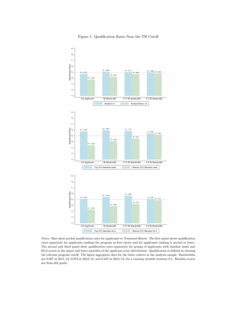
Figure 1: Qualification Rates Near the TH Cutoff

1� �����

1� �����

1� �����

1� ����

1� �����

1� ����1� �����

1� ������

����

����

����

����

4XDOLILFDWLRQ�5DWH

$OO�$SSOLFDQWV ,.�%DQGZLGWK �����,.�%DQGZLGWK ����,.�%DQGZLGWK

5DQNHG��VW 5DQNHG�EHORZ��VW

1� �����

1� �����

1� �����

1� ����

1� ����

1� ����

1� ����1� ����

����

����

����

����

��

4XDOLILFDWLRQ�5DWH

$OO�$SSOLFDQWV ,.�%DQGZLGWK �����,.�%DQGZLGWK ����,.�%DQGZLGWK

7RS�����%DVHOLQH�PDWK %RWWRP�����%DVHOLQH�PDWK

1� �����

1� �����

1� �����

1� ����

1� ����

1� ����

1� ����1� ����

����

����

����

����

��

4XDOLILFDWLRQ�5DWH

$OO�$SSOLFDQWV ,.�%DQGZLGWK �����,.�%DQGZLGWK ����,.�%DQGZLGWK

7RS�����%DVHOLQH�(/$ %RWWRP�����%DVHOLQH�(/$

Notes: Bars show pooled qualification rates for applicants to Townsend Harris. The first panel shows qualificationrates separately for applicants ranking the program as first choice and for applicants ranking it second or lower.The second and third panel show qualification rates separately for groups of applicants with baseline math andELA scores in the upper and lower quartiles of the applicant score distribution. Qualification is defined as clearingthe relevant program cutoff. The figure aggregates data for the three cohorts in the analysis sample. Bandwidthsare 0.007 in 2011/12, 0.073 in 2012/13, and 0.437 in 2013/14, for a running variable between 0-1. Baseline scoresare from 6th grade.

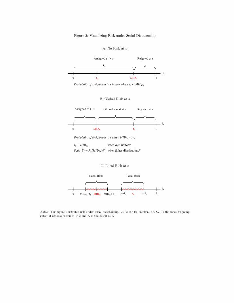
Figure 2: Visualizing Risk under Serial Dictatorship

A. No Risk at s

Probability of assignment to s is zero !ℎ#$ τ% < '()*%

Assigned +′ ≻ + Rejected at s

Ri

0 τs MIDθs 1

B. Global Risk at s

Probability of assignment to s !ℎ#$'()*% < τ%

τ% − '()*% when Ri is uniform

FR(τ%|1) − 3R('()*%|1) when Ri has distribution F

Assigned +′ ≻ + Offered a seat at s Rejected at s

Ri

0 MIDθs τs 1

C. Local Risk at s

Local Risk

Ri

0 MIDθs-51MIDθs MIDθs+51 τs–52 τs

τs+52

Local Risk

1

////////////////////////////// //////////////////////////////

Notes: This figure illustrates risk under serial dictatorship. Ri is the tie-breaker. MID✓s is the most forgiving

cutoff at schools preferred to s and ⌧s is the cutoff at s.

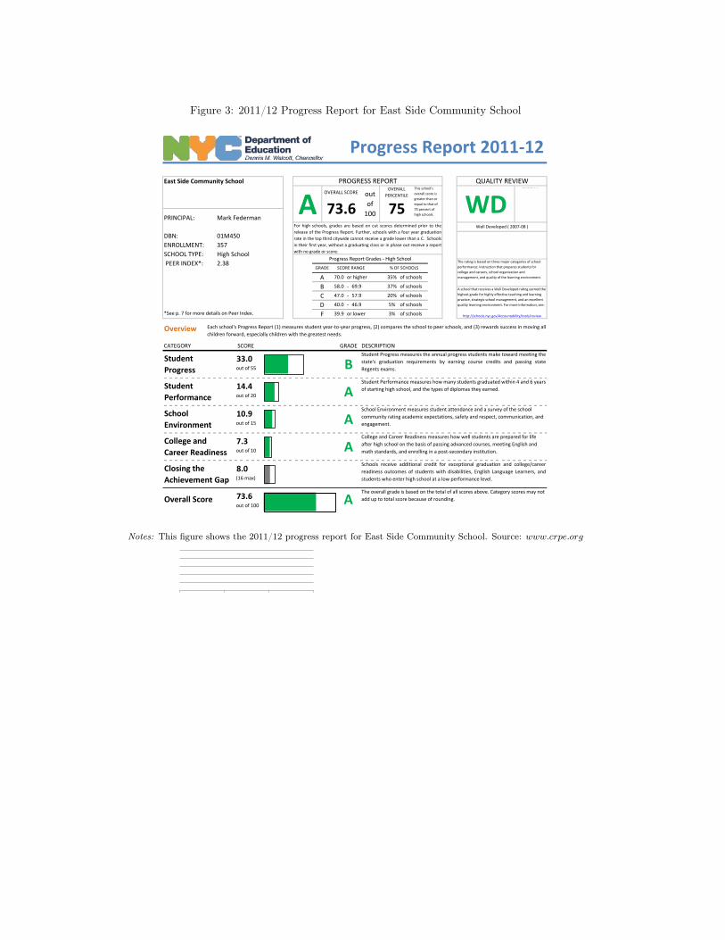
Figure 3: 2011/12 Progress Report for East Side Community School

College and Career Readiness

7.3out of 10 A

College and Career Readiness measures how well students are prepared for life after high school on the basis of passing advanced courses, meeting English and math standards, and enrolling in a post-secondary institution.

*See p. 7 for more details on Peer Index.

of schools

School Environment

Overview

CATEGORY SCORE GRADE

10.9 A

DESCRIPTION

F 39.9

20% of schools

D 40.0 - 46.9 5%

OVERALL PERCENTILE

RANK

75

East Side Community School

01M450

PRINCIPAL:

DBN:

Mark Federman

37%

357High School2.38 PEER INDEX*:

ENROLLMENT:SCHOOL TYPE:

out of 55

Student Performance

14.4 A

47.0 - 57.9

A 70.0

C

OVERALL

SCORE

Each school's Progress Report (1) measures student year-to-year progress, (2) compares the school to peer schools, and (3) rewards success in moving allchildren forward, especially children with the greatest needs.

Student Performance measures how many students graduated within 4 and 6 years of starting high school, and the types of diplomas they earned.

out of 20

http://schools.nyc.gov/ProgressReport

Strong Progress Report results are the basis for recognition and potential rewards for school leaders, and poor results are an important factor in determining whether schools require intensive support or intervention. For more information, see:

http://schools.nyc.gov/community/planning/Support+and+Intervention.htm

92 - 100 72 - 91

GRADE SCORE RANGE % OF SCHOOLS

or lower 3%

A school that receives a Well Developed rating earned the highest grade for highly effective teaching and learning practice, strategic school management, and an excellent quality learning environment. For more information, see:of schools

of schools

B 58.0 - 69.9

School Environment measures student attendance and a survey of the school community rating academic expectations, safety and respect, communication, and engagement.out of 15

out of 100

Closing the Achievement Gap

8.0

The Progress Report is a one-year snapshot of a school’s performance. The Progress Report methodology has evolved over time in response to school and community feedback, changes in state policy, and higher standards. For a description of methodology changes, visit:

Performance Over Time

State Accountability

Percentile rank of this school's overall Progress Report score for the past three years:

The school's current status: In Good Standing

Progress Report Implications

This designation is determined by the New York State Department of Education under theElementary and Secondary Education Act (ESEA) Flexibility Waiver. More information on NewYork State accountability can be found here:

http://schools.nyc.gov/Accountability/tools/accountability/default.htm

Schools receive additional credit for exceptional graduation and college/careerreadiness outcomes of students with disabilities, English Language Learners, andstudents who enter high school at a low performance level.(16 max)

Overall Score 73.6 AThe overall grade is based on the total of all scores above. Category scores may not add up to total score because of rounding.

out of 100

Student Progress

33.0 BStudent Progress measures the annual progress students make toward meeting thestate's graduation requirements by earning course credits and passing stateRegents exams.

http://schools.nyc.gov/Accountability/tools/review

Progress Report 2011-12

AOVERALL SCORE

This school's overall score is greater than or equal to that of 75 percent of high schools.

out of

100

Progress Report Grades - High School 47 - 71

73.6For high schools, grades are based on cut scores determined prior to therelease of the Progress Report. Further, schools with a four year graduationrate in the top third citywide cannot receive a grade lower than a C. Schoolsin their first year, without a graduating class or in phase out receive a reportwith no grade or score.

25 - 46The rating is based on three major categories of school performance: instruction that prepares students for college and careers, school organization and management, and quality of the learning environment.

PROGRESS REPORT QUALITY REVIEW

WDWell Developed ( 2007-08 )

RATING SCORE RANGE

Well DevelopedProficient

DevelopingUnderdeveloped

or higher 35%

of schools

88 8575

0

20

40

60

80

100

2010 2011 2012

Notes: This figure shows the 2011/12 progress report for East Side Community School. Source: www.crpe.org

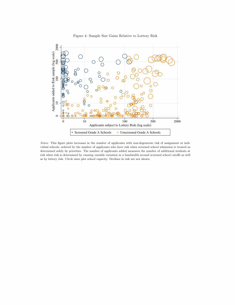
Figure 4: Sample Size Gains Relative to Lottery Risk

���

���

���

����

$SSOLFDQWV�DGGHG�WR�5LVN�VDPSOH��ORJ�VFDOH�

� �� ��� ��� ����

$SSOLFDQWV�VXEMHFW�WR�/RWWHU\�5LVN��ORJ�VFDOH�

6FUHHQHG�*UDGH�$�6FKRROV 8QVFUHHQHG�*UDGH�$�6FKRROV

Notes: This figure plots increases in the number of applicants with non-degenerate risk of assignment at indi-

vidual schools, ordered by the number of applicants who have risk when screened school admission is treated as

determined solely by priorities. The number of applicants added measures the number of additional students at

risk when risk is determined by running variable variation in a bandwidth around screened school cutoffs as well

as by lottery risk. Circle sizes plot school capacity. Declines in risk are not shown.

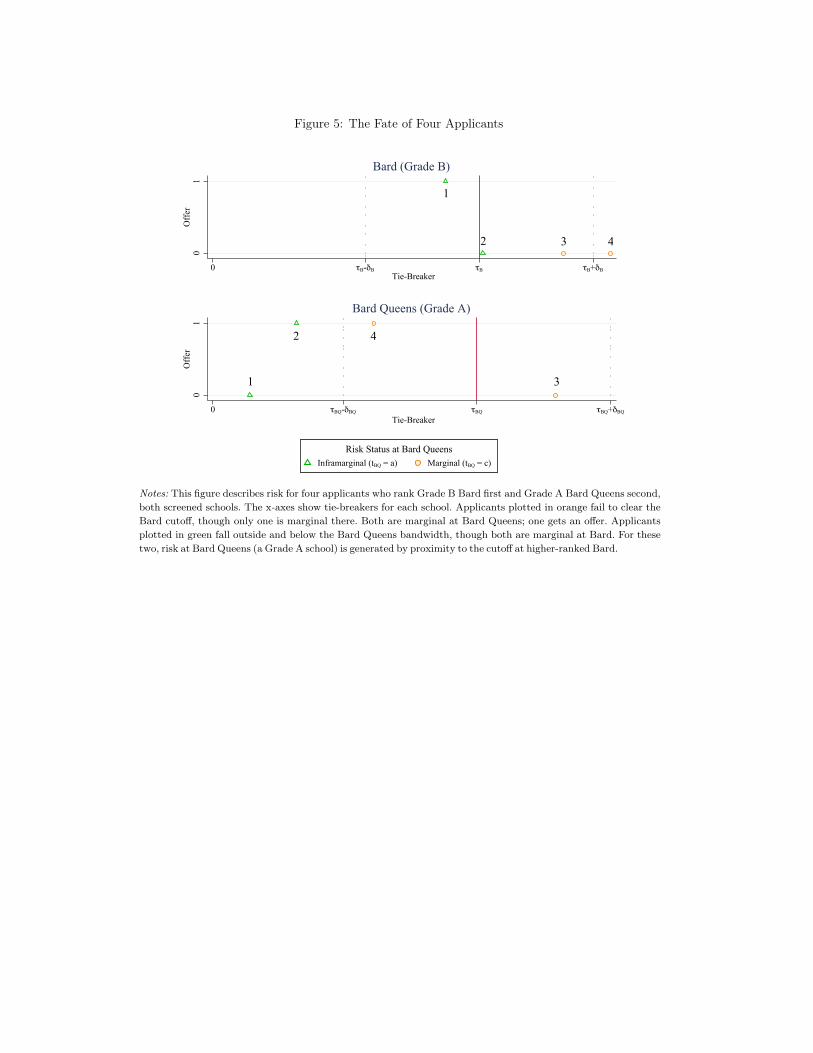
Figure 5: The Fate of Four Applicants

��

2IIHU

� τ%�δ% τ% τ%�δ%Tie-Breaker

%DUG��*UDGH�%�

��

2IIHU

� τ%4�δ%4 τ%4 τ%4�δ%4Tie-Breaker

%DUG�4XHHQV��*UDGH�$�

,QIUDPDUJLQDO��W%4� �D� 0DUJLQDO��W%4� �F�

5LVN�6WDWXV�DW�%DUG�4XHHQV

Notes: This figure describes risk for four applicants who rank Grade B Bard first and Grade A Bard Queens second,

both screened schools. The x axes show tie-breakers for each school. Applicants plotted in orange fail to clear the

Bard cutoff, though only one is marginal there. Both are marginal at Bard Queens; one gets an offer. Applicants

plotted in green fall outside and below the Bard Queens bandwidth, though both are marginal at Bard. For these

two, risk at Bard Queens (a Grade A school) is generated by proximity to the cutoff at higher-ranked Bard.

1

1

2 3 4

3

2 4

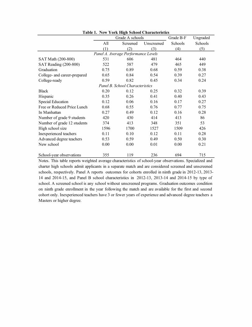
All Screened Unscreened(1) (2) (3) (4) (5)

SAT Math (200-800) 531 606 481 464 440SAT Reading (200-800) 522 587 479 465 449Graduation 0.75 0.89 0.68 0.59 0.38College- and career-prepared 0.65 0.84 0.54 0.39 0.27College-ready 0.59 0.82 0.45 0.34 0.24

Black 0.20 0.12 0.25 0.32 0.39Hispanic 0.35 0.26 0.41 0.40 0.43Special Education 0.12 0.06 0.16 0.17 0.27Free or Reduced Price Lunch 0.68 0.55 0.76 0.77 0.75In Manhattan 0.27 0.49 0.12 0.16 0.28Number of grade 9 students 420 430 414 413 86Number of grade 12 students 374 413 348 351 53High school size 1596 1700 1527 1509 426Inexperienced teachers 0.11 0.10 0.12 0.11 0.28Advanced degree teachers 0.53 0.59 0.49 0.50 0.30New school 0.00 0.00 0.01 0.00 0.21

School-year observations 355 119 236 694 715Notes. This table reports weighted average characteristics of school-year observations. Specialized andcharter high schools admit applicants in a separate match and are considered screened and unscreenedschools, respectively. Panel A reports outcomes for cohorts enrolled in ninth grade in 2012-13, 2013-14 and 2014-15, and Panel B school characteristics in 2012-13, 2013-14 and 2014-15 by type ofschool. A screened school is any school without unscreened programs. Graduation outcomes conditionon ninth grade enrollment in the year following the match and are available for the first and secondcohort only. Inexperienced teachers have 3 or fewer years of experience and advanced degree teachers aMasters or higher degree.

Table 1. New York High School CharacteristicsGrade A schools Grade B-F

SchoolsUngraded

Schools

Panel A. Average Performance Levels

Panel B. School Characteristics

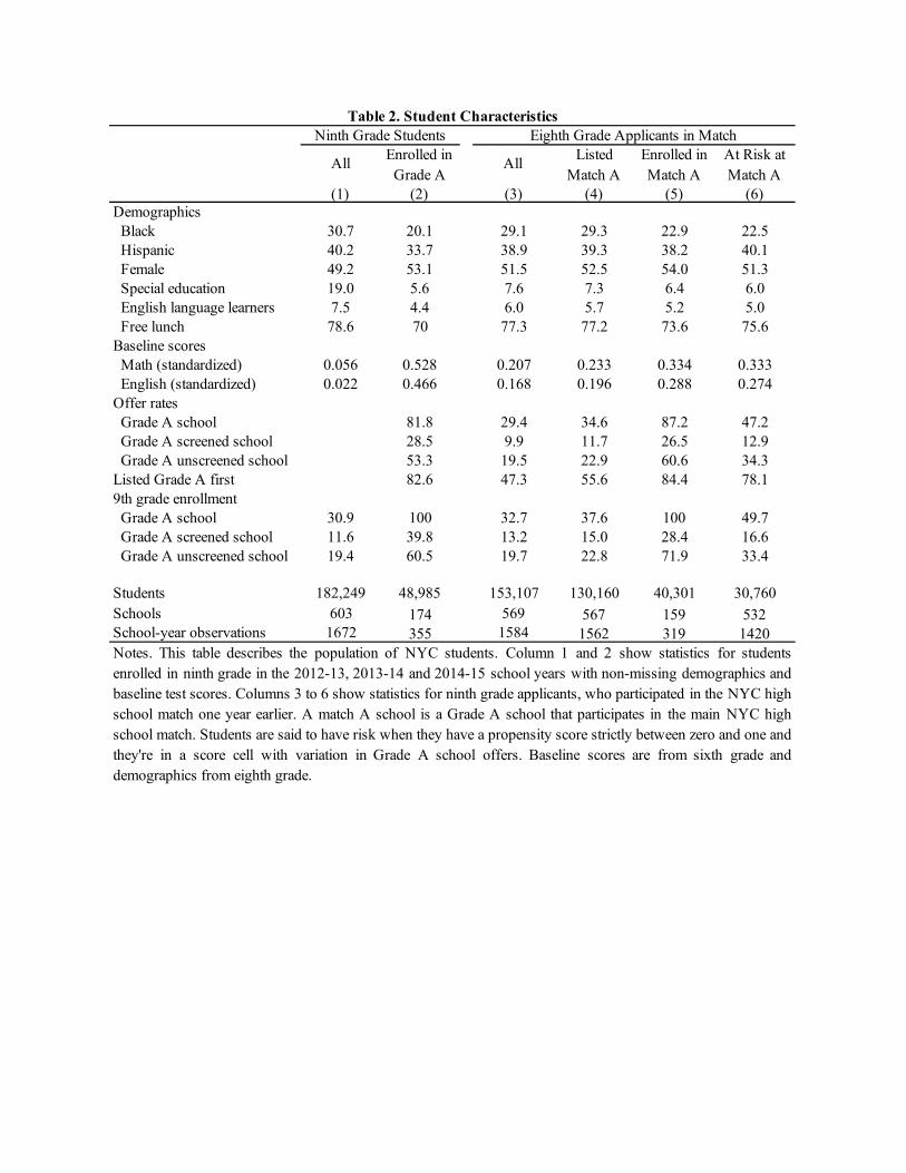
(1) (2) (3) (4) (5) (6)

Black 30.7 20.1 29.1 29.3 22.9 22.5Hispanic 40.2 33.7 38.9 39.3 38.2 40.1Female 49.2 53.1 51.5 52.5 54.0 51.3Special education 19.0 5.6 7.6 7.3 6.4 6.0English language learners 7.5 4.4 6.0 5.7 5.2 5.0Free lunch 78.6 70 77.3 77.2 73.6 75.6

Math (standardized) 0.056 0.528 0.207 0.233 0.334 0.333English (standardized) 0.022 0.466 0.168 0.196 0.288 0.274

Grade A school 81.8 29.4 34.6 87.2 47.2Grade A screened school 28.5 9.9 11.7 26.5 12.9Grade A unscreened school 53.3 19.5 22.9 60.6 34.3

Listed Grade A first 82.6 47.3 55.6 84.4 78.1

Grade A school 30.9 100 32.7 37.6 100 49.7Grade A screened school 11.6 39.8 13.2 15.0 28.4 16.6Grade A unscreened school 19.4 60.5 19.7 22.8 71.9 33.4

Students 182,249 48,985 153,107 130,160 40,301 30,760Schools 603 174 569 567 159 532School-year observations 1672 355 1584 1562 319 1420

Table 2. Student CharacteristicsNinth Grade Students Eighth Grade Applicants in Match

All Enrolled in Grade A

All Listed Match A

Enrolled in Match A

At Risk at Match A

Demographics

Baseline scores

Offer rates

9th grade enrollment

Notes. This table describes the population of NYC students. Column 1 and 2 show statistics for studentsenrolled in ninth grade in the 2012-13, 2013-14 and 2014-15 school years with non-missing demographics andbaseline test scores. Columns 3 to 6 show statistics for ninth grade applicants, who participated in the NYC highschool match one year earlier. A match A school is a Grade A school that participates in the main NYC highschool match. Students are said to have risk when they have a propensity score strictly between zero and one and they're in a score cell with variation in Grade A school offers. Baseline scores are from sixth grade anddemographics from eighth grade.

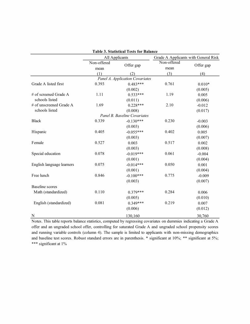
(1) (2) (3) (4)

Grade A listed first 0.393 0.483*** 0.761 0.010*(0.002) (0.005)

# of screened Grade A 1.11 0.533*** 1.19 0.005 schools listed (0.011) (0.006)# of unscreened Grade A 1.69 0.228*** 2.10 -0.012 schools listed (0.008) (0.017)

Black 0.339 -0.130*** 0.230 -0.003 (0.003) (0.006)

Hispanic 0.405 -0.055*** 0.402 0.005 (0.003) (0.007)

Female 0.527 0.003 0.517 0.002(0.003) (0.008)

Special education 0.078 -0.019*** 0.061 -0.004(0.001) (0.004)

English language learners 0.075 -0.014*** 0.050 0.001(0.001) (0.004)

Free lunch 0.846 -0.100*** 0.775 -0.009(0.003) (0.007)

Baseline scoresMath (standardized) 0.110 0.379*** 0.284 0.006

(0.005) (0.010)English (standardized) 0.081 0.349*** 0.219 0.007

(0.006) (0.012)

N 130,160 30,760

Panel A. Application Covariates

Panel B. Baseline Covariates

Notes. This table reports balance statistics, computed by regressing covariates on dummies indicating a Grade Aoffer and an ungraded school offer, controlling for saturated Grade A and ungraded school propensity scoresand running variable controls (column 4). The sample is limited to applicants with non-missing demographicsand baseline test scores. Robust standard errors are in parenthesis. * significant at 10%; ** significant at 5%;*** significant at 1%

Table 3. Statistical Tests for BalanceAll Applicants Grade A Applicants with General Risk

Non-offered mean

Offer gapNon-offered

mean Offer gap

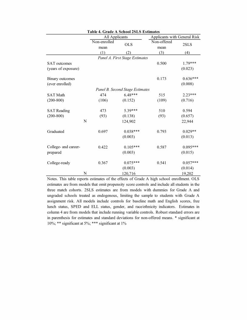
(1) (2) (3) (4)

SAT outcomes 0.500 1.79***(years of exposure) (0.023)

0.173 0.636***(ever enrolled) (0.008)

474 6.48*** 515 2.23***(200-800) (106) (0.152) (109) (0.716)

473 5.39*** 510 0.594(200-800) (93) (0.138) (93) (0.657)

N 124,902 22,944

0.697 0.038*** 0.793 0.029**(0.003) (0.013)

0.422 0.105*** 0.587 0.095***(0.003) (0.015)

0.367 0.075*** 0.541 0.057***(0.003) (0.014)

N 120,716 19,202

Table 4. Grade A School 2SLS EstimatesAll Applicants Applicants with General Risk

Non-enrolledmean

OLSNon-offered

mean2SLS

Graduated

College- and career-prepared

College-ready

Notes. This table reports estimates of the effects of Grade A high school enrollment. OLSestimates are from models that omit propensity score controls and include all students in thethree match cohorts. 2SLS estimates are from models with dummies for Grade A andungraded schools treated as endogenous, limiting the sample to students with Grade Aassignment risk. All models include controls for baseline math and English scores, freelunch status, SPED and ELL status, gender, and race/ethnicity indicators. Estimates incolumn 4 are from models that include running variable controls. Robust standard errors arein parenthesis for estimates and standard deviations for non-offered means. * significant at10%; ** significant at 5%; *** significant at 1%

Binary outcomes

SAT Math

SAT Reading

Panel A. First Stage Estimates

Panel B. Second Stage Estimates

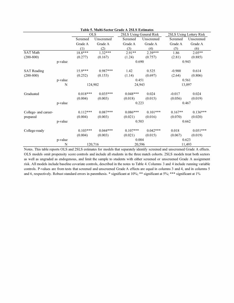
(1) (2) (3) (4) (5) (6) SAT Math 18.8*** 1.32*** 2.91** 2.39*** 1.86 2.05**(200-800) (0.277) (0.167) (1.24) (0.757) (2.81) (0.885)

p-value

SAT Reading 15.9*** 0.987*** 1.42 0.525 -0.900 0.614(200-800) (0.252) (0.153) (1.14) (0.697) (2.64) (0.806)

p-valueN

Graduated 0.018*** 0.035*** 0.048*** 0.024 -0.017 0.024(0.004) (0.003) (0.018) (0.015) (0.056) (0.019)

p-value

College- and career- 0.112*** 0.087*** 0.086*** 0.101*** 0.167** 0.136***prepared (0.004) (0.003) (0.021) (0.016) (0.070) (0.020)

p-value

College-ready 0.103*** 0.044*** 0.107*** 0.042*** 0.018 0.051***(0.004) (0.003) (0.021) (0.015) (0.067) (0.019)

p-valueN

Table 5. Multi-Sector Grade A 2SLS EstimatesOLS 2SLS Using General Risk 2SLS Using Lottery Risk

ScreenedGrade A

UnscreenedGrade A

ScreenedGrade A

UnscreenedGrade A

ScreenedGrade A

UnscreenedGrade A

0.503 0.662

0.690 0.943

0.451 0.561124,902 24,943 13,097

0.223 0.467

0.004 0.623120,716 20,596 11,493

Notes. This table reports OLS and 2SLS estimates for models that separately identify screened and unscreened Grade A effects.OLS models omit propensity score controls and include all students in the three match cohorts. 2SLS models treat both sectorsas well as ungraded as endogenous, and limit the sample to students with either screened or unscreened Grade A assignmentrisk. All models include baseline covariate controls, described in the notes to Table 4. Columns 3 and 4 include running variablecontrols. P-values are from tests that screened and unscreened Grade A effects are equal in columns 3 and 4, and in columns 5and 6, respectively. Robust standard errors in parenthesis. * significant at 10%; ** significant at 5%; *** significant at 1%

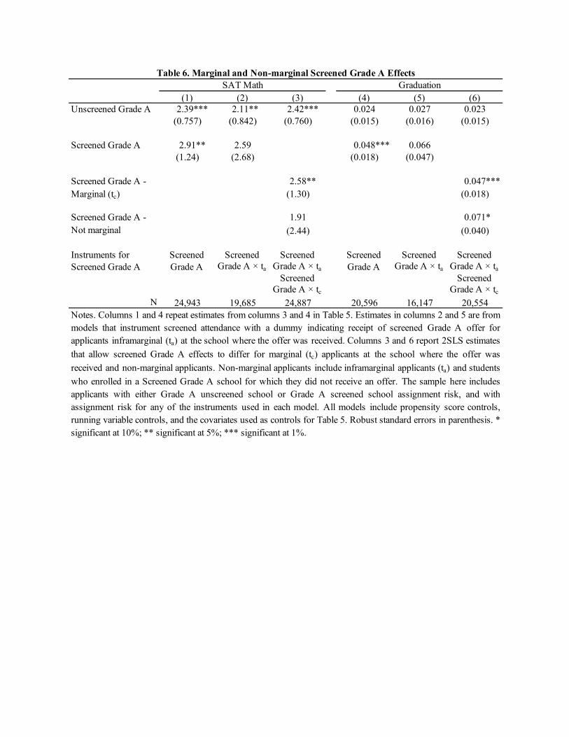
(1) (2) (3) (4) (5) (6) Unscreened Grade A 2.39*** 2.11** 2.42*** 0.024 0.027 0.023

(0.757) (0.842) (0.760) (0.015) (0.016) (0.015)

Screened Grade A 2.91** 2.59 0.048*** 0.066(1.24) (2.68) (0.018) (0.047)

Screened Grade A - 2.58** 0.047***Marginal (tc) (1.30) (0.018)

Screened Grade A - 1.91 0.071*Not marginal (2.44) (0.040)

Instruments for Screened Screened Screened Screened Screened ScreenedScreened Grade A Grade A Grade A × ta Grade A × ta Grade A Grade A × ta Grade A × ta

Screened ScreenedGrade A × tc Grade A × tc

N 24,943 19,685 24,887 20,596 16,147 20,554

Table 6. Marginal and Non-marginal Screened Grade A EffectsSAT Math Graduation

Notes. Columns 1 and 4 repeat estimates from columns 3 and 4 in Table 5. Estimates in columns 2 and 5 are from models that instrument screened attendance with a dummy indicating receipt of screened Grade A offer forapplicants inframarginal (ta) at the school where the offer was received. Columns 3 and 6 report 2SLS estimatesthat allow screened Grade A effects to differ for marginal (tc) applicants at the school where the offer wasreceived and non-marginal applicants. Non-marginal applicants include inframarginal applicants (ta) and studentswho enrolled in a Screened Grade A school for which they did not receive an offer. The sample here includesapplicants with either Grade A unscreened school or Grade A screened school assignment risk, and withassignment risk for any of the instruments used in each model. All models include propensity score controls,running variable controls, and the covariates used as controls for Table 5. Robust standard errors in parenthesis. * significant at 10%; ** significant at 5%; *** significant at 1%.

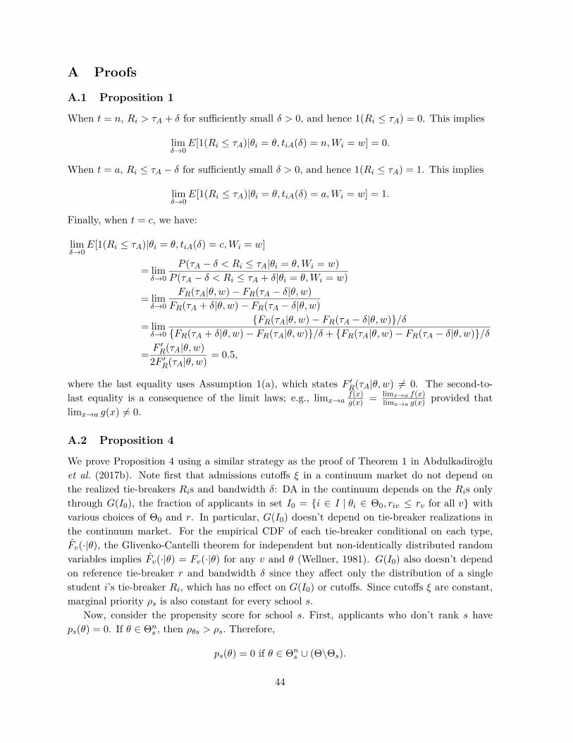
A Proofs

A.1 Proposition 1

When t = n, Ri

> ⌧

A

+ � for su�ciently small � > 0, and hence 1(R

i

⌧

A

) = 0. This implies

lim

�!0E[1(R

i

⌧

A

)|✓i

= ✓, t

iA

(�) = n,W

i

= w] = 0.

When t = a, Ri

⌧

A

� � for su�ciently small � > 0, and hence 1(R

i

⌧

A

) = 1. This implies

lim

�!0E[1(R

i

⌧

A

)|✓i

= ✓, t

iA

(�) = a,W

i

= w] = 1.

Finally, when t = c, we have:

lim

�!0E[1(R

i

⌧

A

)|✓i

= ✓, t

iA

(�) = c,W

i

= w]

= lim

�!0

P (⌧

A

� � < R

i

⌧

A

|✓i

= ✓,W

i

= w)

P (⌧

A

� � < R

i

⌧

A

+ �|✓i

= ✓,W

i

= w)

= lim

�!0

F

R

(⌧

A

|✓, w)� F

R

(⌧

A

� �|✓, w)F

R

(⌧

A

+ �|✓, w)� F

R

(⌧

A

� �|✓, w)

= lim

�!0

{FR

(⌧

A

|✓, w)� F

R

(⌧

A

� �|✓, w)}/�{F

R

(⌧

A

+ �|✓, w)� F

R

(⌧

A

|✓, w)}/� + {FR

(⌧

A

|✓, w)� F

R

(⌧

A

� �|✓, w)}/�

=

F

0R

(⌧

A

|✓, w)2F

0R

(⌧

A

|✓, w) = 0.5,

where the last equality uses Assumption 1(a), which states F

0R

(⌧

A

|✓, w) 6= 0. The second-to-last equality is a consequence of the limit laws; e.g., lim

x!a

f(x)g(x) =

limx!a

f(x)lim

x!a

g(x) provided thatlim

x!a

g(x) 6= 0.

A.2 Proposition 4

We prove Proposition 4 using a similar strategy as the proof of Theorem 1 in Abdulkadiro�luet al. (2017b). Note first that admissions cuto�s ⇠ in a continuum market do not depend onthe realized tie-breakers R

i

s and bandwidth �: DA in the continuum depends on the R

i

s onlythrough G(I0), the fraction of applicants in set I0 = {i 2 I | ✓

i

2 ⇥0, riv r

v

for all v} withvarious choices of ⇥0 and r. In particular, G(I0) doesn’t depend on tie-breaker realizations inthe continuum market. For the empirical CDF of each tie-breaker conditional on each type,ˆ

F

v

(·|✓), the Glivenko-Cantelli theorem for independent but non-identically distributed randomvariables implies ˆ

F

v

(·|✓) = F

v

(·|✓) for any v and ✓ (Wellner, 1981). G(I0) also doesn’t dependon reference tie-breaker r and bandwidth � since they a�ect only the distribution of a singlestudent i’s tie-breaker R

i

, which has no e�ect on G(I0) or cuto�s. Since cuto�s ⇠ are constant,marginal priority ⇢

s

is also constant for every school s.Now, consider the propensity score for school s. First, applicants who don’t rank s have

p

s

(✓) = 0. If ✓ 2 ⇥

n

s

, then ⇢

✓s

> ⇢

s

. Therefore,

p

s

(✓) = 0 if ✓ 2 ⇥

n

s

[ (⇥\⇥s

).

44

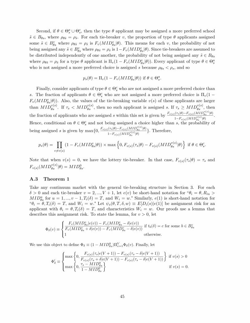
Second, if ✓ 2 ⇥

a

s

[ ⇥

c

s

, then the type ✓ applicant may be assigned a more preferred schools̃ 2 B

✓s

, where ⇢✓s̃

= ⇢

s̃

. For each tie-breaker v, the proportion of type ✓ applicants assignedsome s̃ 2 B

v

✓s

where ⇢✓s̃

= ⇢

s̃

is F

v

(MID

v

✓s

|✓). This means for each v, the probability of notbeing assigned any s̃ 2 B

v

✓s

where ⇢✓s̃

= ⇢

s̃

is 1�F

v

(MID

v

✓s

|✓). Since tie-breakers are assumed tobe distributed independently of one another, the probability of not being assigned any s̃ 2 B

✓s

where ⇢✓s̃

= ⇢

s̃

for a type ✓ applicant is ⇧

v

(1� F

v

(MID

v

✓s

|✓)). Every applicant of type ✓ 2 ⇥

a

s

who is not assigned a more preferred choice is assigned s because ⇢✓s

< ⇢

s

, and so

p

s

(✓) = ⇧

v

(1� F

v

(MID

v

✓s

|✓)) if ✓ 2 ⇥

a

s

.

Finally, consider applicants of type ✓ 2 ⇥

c

s

who are not assigned a more preferred choice thans. The fraction of applicants ✓ 2 ⇥

c

s

who are not assigned a more preferred choice is ⇧

v

(1 �F

v

(MID

v

✓s

|✓)). Also, the values of the tie-breaking variable v(s) of these applicants are largerthan MID

v(s)✓s

. If ⌧s

< MID

v(s)✓s

, then no such applicant is assigned s. If ⌧s

� MID

v(s)✓s

, then

the fraction of applicants who are assigned s within this set is given by F

v(s)(⌧s|✓)�F

v(s)(MID

v(s)✓s

|✓)1�F

v(s)(MID

v(s)✓s

|✓).

Hence, conditional on ✓ 2 ⇥

c

s

and not being assigned a choice higher than s, the probability ofbeing assigned s is given by max{0, Fv(s)(⌧s|✓)�F

v(s)(MID

v(s)✓s

|✓)1�F

v(s)(MID

v(s)✓s

|✓)}. Therefore,

p

s

(✓) =

Y

v 6=v(s)

(1� F

v

(MID

v

✓s

|✓))⇥max

n

0, F

v(s)(⌧s|✓)� F

v(s)(MID

v(s)✓s

|✓)o

if ✓ 2 ⇥

c

s

.

Note that when v(s) = 0, we have the lottery tie-breaker. In that case, F

v(s)(⌧s|✓) = ⌧

s

andF

v(s)(MID

v(s)✓s

|✓) = MID

0✓s

.

A.3 Theorem 1Take any continuum market with the general tie-breaking structure in Section 3. For each� > 0 and each tie-breaker v = 2, ..., V + 1, let e(v) be short-hand notation for “✓

i

= ✓, R

iu

>

MID

u

✓s

for u = 1, ..., v � 1, T

i

(�) = T, and W

i

= w." Similarly, e(1) is short-hand notation for“✓

i

= ✓, T

i

(�) = T, and W

i

= w." Let s

(✓, T, �, w) ⌘ E[D

i

(s)|e(1)] be assignment risk for anapplicant with ✓

i

= ✓, T

i

(�) = T, and characteristics W

i

= w. Our proofs use a lemma thatdescribes this assignment risk. To state the lemma, for v > 0, let

��(v) ⌘

8

>

<

>

:

Fv(MID

v✓s|e(v))� Fv(MID

v✓s � �|e(v))

Fv(MID

v✓s + �|e(v))� Fv(MID

v✓s � �|e(v)) if tb(�) = c for some b 2 B

v✓s

1 otherwise.

We use this object to define �� ⌘ (1�MID

0✓s)⇧

Vv=1��(v). Finally, let

�

0� ⌘

8

>

>

<

>

>

:

max

⇢

0,

Fv(s)(⌧s|e(V + 1))� Fv(s)(⌧s � �|e(V + 1))

Fv(s)(⌧s + �|e(V + 1))� Fv(s)(⌧s � �|e(V + 1))

�

if v(s) > 0

max

⇢

0,

⌧s �MID

0✓s

1�MID

0✓s

�

if v(s) = 0.

45

Lemma 1. In the general tie-breaking setting of Section 3, for any fixed � > 0 such that� < min

✓,s,v

|⌧s

�MID

v

✓,s

|, we have:

s

(✓, T, �, w) =

8

>

<

>

:

0 if ts

(�) = n or t

b

(�) = a for some b 2 B

✓s

,

�

�

otherwise and t

s

(�) = a,

�

�

⇥ �

0�

otherwise and t

s

(�) = c.

Proof of Lemma 1. We start verifying the first line in

s

(✓, T, �, w). Applicants who don’t lists have

s

(✓, T, �, w) = 0. Among those who list s, those of ts

(�) = n have ✓ 2 ⇥

n

s

or, if v(s) 6=0, ✓ 2 ⇥

c

s

and R

iv(s) > ⌧

s

+ �. If ✓ 2 ⇥

n

s

, then ⇢

✓s

> ⇢

s

so that s

(✓, T, �, w) = 0. Even if✓ 62 ⇥

n

s

, as long as ✓ 2 ⇥

c

s

and R

iv(s) > ⌧

s

+ �, student i never clears the cuto� at school s so

s

(✓, T, �, w) = 0.To show the remaining cases, take as given that it is not the case that t

s

(�) = n or t

b

(�) =

a for some b 2 B

✓s

. Applicants with t

b

(�) 6= a for all b 2 B

✓s

and t

s

(�) = a or c may be assignedb 2 B

✓s

, where ⇢✓b

= ⇢

b

. Since the (aggregate) distribution of tie-breaking variables for type✓ students is ˆ

F

v

(·|✓) = F

v

(·|✓), conditional on T

i

(�) = T , the proportion of type ✓ applicantsnot assigned any b 2 B

✓s

where ⇢✓b

= ⇢

b

is �

�

= (1 �MID

0✓s

)⇧

v

�

�

(v) since each �

�

(v) is theprobability of not being assigned to any b 2 B

v

✓s

. To see why �

�

(v) is the probability of not beingassigned to any b 2 B

v

✓s

, note that if tb

(�) 6= c for all b 2 B

v

✓s

, then t

b

(�) = n for all b 2 B

v

✓s

sothat applicants are never assigned to any b 2 B

v

✓s

. Otherwise, i.e., if tb

(�) = c for some b 2 B

v

✓s

,then applicants are assigned to s if and only if their values of tie-breaker v clear the cuto� ofthe school that produces MID

v

✓s

, where applicants have t

s

(�) = c. This event happens withprobability

F

v

(MID

v

✓s

|e(v))� F

v

(MID

v

✓s

� �|e(v))F

v

(MID

v

✓s

+ �|e(v))� F

v

(MID

v

✓s

� �|e(v)) ,

implying that �

�

(v) is the probability of not being assigned to any b 2 B

v

✓s

.Given this fact, to see the second line, note that every applicant of type t

s

(�) = a who is notassigned a higher choice is assigned s for sure because ⇢

✓s

< ⇢

s

or ⇢✓s

+ R

iv(s) < ⇠

s

. Therefore,we have

s

(✓, T, �, w) = �

�

.

Finally, consider applicants with t

s

(�) = c. The fraction of those who are not assigned ahigher choice is �

�

, as explained above. Also, for tie-breaker v(s), the tie-breaker values ofthese applicants are larger (worse) than MID

v(s)✓s

. If ⌧s

< MID

v(s)✓s

, then no such applicant isassigned s. If ⌧

s

� MID

v(s)✓s

, then the fraction of applicants who are assigned s conditional on⌧

s

� MID

v(s)✓s

is given by

max

(

0,

F

v(s)(⌧s|e(V + 1))�max{Fv(s)(MID

v(s)✓s

|e(V + 1)), F

v(s)(⌧s � �|e(V + 1))}

F

v(s)(⌧s + �|e(V + 1))�max{Fv(s)(MID

v(s)✓s

|e(V + 1)), F

v(s)(⌧s � �|e(V + 1))}

)

if v(s) 6= 0

andmax

⇢

0,

⌧

s

�MID

0✓s

1�MID

0✓s

�

if v(s) = 0.

46

If MID

v(s)✓s

< ⌧

s

, then � < min

✓,s,v

|⌧s

�MID

v

✓,s

| implies MID

v(s)✓s

< ⌧

s

� �. This in turn implies

max{Fv(s)(MID

v(s)✓s

|e(V + 1)), F

v(s)(⌧s � �|e(V + 1))} = F

v(s)(⌧s � �|e(V + 1)).

If MID

v(s)✓s

> ⌧

s

, then � < min

✓,s,v

|⌧s

�MID

v

✓,s

| implies MID

v(s)✓s

> ⌧

s

+ �. By the definition ofe(V +1), R

iu

> MID

u

✓s

for u = 1, ..., V . Therefore, there is no applicant with R

iv(s) > MID

v(s)✓s

and R

iv(s) 2 [⌧

s

� �, ⌧

s

+ �].Hence, conditional on t

s

(�) = c and not being assigned a choice more preferred than s, theprobability of being assigned s is given by �

0�

. Therefore, for students with t

s

(�) = c, we have

s

(✓, T, �, w) = �

�

⇥ �

0�

.

Lemma 2. In the general tie-breaking setting of Section 3, for all s, ✓, and su�ciently small� > 0, we have:

s

(✓, T, �, w) =

8

>

>

>

>

>

>

>

>

>

>

>

<

>

>

>

>

>

>

>

>

>

>

>

:

0 if ts

(0) = n or t

b

(0) = a for some b 2 B

✓s

,

�

⇤�

otherwise and t

s

(0) = a,

�

⇤�

⇥F

v(s)(⌧s|e(V + 1))� F

v(s)(⌧s � �|e(V + 1))

F

v(s)(⌧s + �|e(V + 1))� F

v(s)(⌧s � �|e(V + 1))

otherwise and t

s

(0) = c and v(s) 6= 0.

�

⇤�

⇥ max{0,⌧

s

�MID

0✓s

1�MID

0✓s

}

otherwise and t

s

(0) = c and v(s) = 0.

(17)

where

�

⇤�

(v) ⌘

8

>

<

>

:

F

v

(MID

v

✓s

+ �|e(v))� F

v

(MID

v

✓s

|e(v))F

v

(MID

v

✓s

+ �|e(v))� F

v

(MID

v

✓s

� �|e(v)) if MID

v

✓s

= ⌧

b

and t

b

= c for some b 2 B

v

✓s

,

1 otherwise

and

�

⇤�

⌘ (1�MID

0✓s

)⇧

V

v=1�⇤�

(v).

Proof of Lemma 2. The first line follows from Lemma 1 and the fact that t

s

(0) = n or t

b

(0) =

a for some b 2 B

✓s

imply t

s

(�) = n or t

b

(�) = a for some b 2 B

✓s

for su�ciently small � > 0.For the remaining lines, first note that conditional on t

s

(0) 6= n and t

b

(0) 6= a for all b 2 B

✓s

,we have �

⇤�

(v) = �

�

(v) and so �

⇤�

= �

�

holds for small enough �. �

⇤�

therefore is the probabilityof not being assigned to a school preferred to s in the last three cases.

The second line is then by the fact that t

s

(0) = a implies t

s

(�) = a for small enough � > 0.The third line is by the fact that for small enough � > 0,

�

0�

= max

⇢

0,

F

v(s)(⌧s|e(V + 1))� F

v(s)(⌧s � �|e(V + 1))

F

v(s)(⌧s + �|e(V + 1))� F

v(s)(⌧s � �|e(V + 1))

�

=

F

v(s)(⌧s|e(V + 1))� F

v(s)(⌧s � �|e(V + 1))

F

v(s)(⌧s + �|e(V + 1))� F

v(s)(⌧s � �|e(V + 1))

,

47

where we invoke Assumption 1(b), which implies MID

v

✓s

6= ⌧

s

. The last line directly followsfrom Lemma 1.

We use Lemma 2 to derive Theorem 1. We characterize lim

�!0 s

(✓, T, �, w) and show that itcoincides with

s

(✓, T ) in the main text. In the first case in Lemma 2, s

(✓, T, �, w) is constant(0) for any small enough �. The constant value is also lim

�!0 s

(✓, T, �, w) in this case.To characterize lim

�!0 s

(✓, T, �, w) in the remaining cases, note that by the di�erentiabilityof F

v

(·|e(v)) (recall Assumption 1), L’Hopital’s rule implies:

lim

�!0

F

v(s)(⌧s|e(V + 1))� F

v(s)(⌧s � �|e(V + 1))

F

v(s)(⌧s + �|e(V + 1))� F

v(s)(⌧s � �|e(V + 1))

=

F

0v(s)(⌧s|e(V + 1))

2F

0v(s)(⌧s|e(V + 1))

= 0.5

andlim

�!0

F

v

(MID

v

✓s

+ �|e(v))� F

v

(MID

v

✓s

|e(v))F

v

(MID

v

✓s

+ �|e(v))� F

v

(MID

v

✓s

� �|e(v)) =

F

0v

(MID

v

✓s

|e(v))2F

0v

(MID

v

✓s

|e(v)) = 0.5.

This implies lim

�!0�⇤�

(v) = 0.5

1{MID

v

✓s

=⌧

b

and t

b

=c for some b2Bv

✓s

} since 1{MID

v

✓s

= ⌧

b

and t

b

=

c for some b 2 B

v

✓s

} does not depend on �. Therefore

lim

�!0�

⇤�

= (1�MID

0✓s

)0.5

m

s

(✓,T )

where m

s

(✓, T ) = |{v > 0 : MID

v

✓s

= ⌧

b

and t

b

= c for some b 2 B

v

✓s

}|.Combining these limiting facts with the fact that the limit of a product of functions equals

the product of the limits of the functions, we obtain the following: lim

�!0 s

(✓, T, �, w) = 0 if(a) t

s

= n or (b) t

b

= a for some b 2 B

✓s

. Otherwise,

lim

�!0

s

(✓, T, �, w) =

8

>

<

>

:

0.5

m

s

(✓,T )(1�MID

0✓s

) if ts

(0) = a

0.5

m

s

(✓,T )max

�

0, ⌧

s

�MID

0✓s

if ts

(0) = c and v(s) = 0

0.5

1+m

s

(✓,T )(1�MID

0✓s

) if ts

(0) = c and v(s) > 0.

This expression coincides with

s

(✓, T ), completing the proof of Theorem 1.

A.4 Theorem 2

Here we prove the following lemmas used in the proof of Theorem 2 in the main text.

Lemma 3. (Cuto� almost sure convergence) ˆ

⇠

N

a.s.�! ⇠ where ⇠ denotes the vector of continuummarket cuto�s.

Lemma 4. (Estimated local propensity score almost sure convergence) For all ✓ 2 ⇥, s 2 S, andT 2 {a, c, n}S, we have ˆ

Ns

(✓, T ; �

N

)

a.s.�!

s

(✓, T ) as N ! 1 and �N

! 0.

Lemma 5. (Bandwidth-specific propensity score almost sure convergence) For all ✓ 2 ⇥, s 2 S,

T 2 {a, c, n}S, and �N

such that �N

! 0 and N�

N

! 1 as N ! 1, we have Ns

(✓, T ; �

N

)

p�!

s

(✓, T ) as N ! 1.

48

Proof of Lemma 3

The proof of Lemma 3 is analogous to the proof of Lemma 3 in Abdulkadiro�lu et al. (2017b)and available upon request. The main di�erence is that to deal with multiple non-lottery tie-breakers, the proof of Lemma 3 needs to invoke Assumption 1 and the Glivenko-Cantelli theoremfor independent but non-identically distributed random variables (Wellner, 1981).

Proof of Lemma 4

ˆ

Ns

(✓, T ; �

N

) is almost everywhere continuous in finite sample cuto�s ˆ

⇠

N

, finite sample MIDs(MID

v

✓s

), and bandwidth �

N

. Since every MID

v

✓s

is almost everywhere continuous in finitesample cuto�s ˆ

⇠

N

, ˆ

Ns

(✓, T ; �

N

) is almost everywhere continuous in finite sample cuto�s ˆ

⇠

N

and bandwidth �

N

. Recall �N

! 0 by assumption while ˆ

⇠

N

a.s.�! ⇠ by Lemma 3. Therefore,by the continuous mapping theorem, as N ! 1, ˆ

Ns

(✓, T ; �

N

) almost surely converges toˆ

Ns

(✓, T ; �

N

) with ⇠ replacing ˆ

⇠

N

, which is s

(✓, T ).

Proof of Lemma 5

We use the following fact, which is implied by Example 19.29 in van der Vaart (2000).

Lemma 6. Let X be a random variable distributed according to some CDF F over [0, 1]. LetF (·|X 2 [x� �, x+ �]) be the conditional version of F conditional on X being in a small window[x � �, x + �] where x 2 [0, 1] and � 2 (0, 1]. Let X1, ..., XN

be iid draws from F . Let ˆ

F

N

bethe empirical CDF of X1, ..., XN

. Let ˆ

F

N

(·|X 2 [x� �, x+ �]) be the conditional version of ˆ

F

N

conditional on a subset of draws falling in [x� �, x+ �], i.e., {Xi

|i = 1, ..., n,X

i

2 [x� �, x+ �]}.Suppose (�

N

) is a sequence with �

N

# 0 and �

N

⇥ N ! 1. Then ˆ

F

N

(·|X 2 [x � �

N

, x + �

N

])

uniformly converges to F (·|X 2 [x� �

N

, x+ �

N

]), i.e.,

sup

x

02[0,1]| ˆF

N

(x

0|X 2 [x� �

N

, x+ �

N

])�F (x

0|X 2 [x� �

N

, x+ �

N

])| !p

0 as N ! 1 and �N

! 0.

Proof of Lemma 6. We first prove the statement for x 2 (0, 1). Let P be the probability measureof X and ˆ

P

N

be the empirical measure of X1, ..., XN

. Note that

sup

x

02[0,1]| ˆF

N

(x

0|X 2 [x� �

N

, x+ �

N

])� F (x

0|X 2 [x� �

N

, x+ �

N

])|

= sup

t2[�1,1]| ˆF

N

(x+ t�

N

|X 2 [x� �

N

, x+ �

N

])� F (x+ t�

N

|X 2 [x� �

N

, x+ �

N

])|

= sup

t2[�1,1]|ˆ

P

N

[x� �

N

, x+ t�

N

]

ˆ

P

N

[x� �

N

, x+ �

N

]

� P

X

[x� �

N

, x+ t�

N

]

P

X

[x� �

N

, x+ �

N

]

|

=

1

ˆ

P

N

[x� �

N

, x+ �

N

]P

X

[x� �

N

, x+ �

N

]

⇥ sup

t2[�1,1]| ˆP

N

[x� �

N

, x+ t�

N

]P

X

[x� �

N

, x+ �

N

]� ˆ

P

N

[x� �

N

, x+ �

N

]P

X

[x� �

N

, x+ t�

N

]|

49

=

1

ˆ

P

N

[x� �

N

, x+ �

N

]P

X

[x� �

N

, x+ �

N

]

⇥ sup

t2[�1,1]| ˆP

N

[x� �

N

, x+ t�

N

](P

X

[x� �

N

, x+ �

N

]� ˆ

P

N

[x� �

N

, x+ �

N

])

+

ˆ

P

N

[x� �

N

, x+ �

N

](

ˆ

P

N

[x� �

N

, x+ t�

N

]� P

X

[x� �

N

, x+ t�

N

])|

1

ˆ

P

N

[x� �

N

, x+ �

N

]P

X

[x� �

N

, x+ �

N

]

⇥ { sup

t2[�1,1]

ˆ

P

N

[x� �

N

, x+ t�

N

]| ˆPN

[x� �

N

, x+ �

N

]� P

X

[x� �

N

, x+ �

N

]|

+ sup

t2[�1,1]

ˆ

P

N

[x� �

N

, x+ �

N

]| ˆPN

[x� �

N

, x+ t�

N

]� P

X

[x� �

N

, x+ t�

N

]|}

=

1

P

X

[x� �

N

, x+ �

N

]

⇥ {| ˆPN

[x� �

N

, x+ �

N

]� P

X

[x� �

N

, x+ �

N

]|+ sup

t2[�1,1]| ˆP

N

[x� �

N

, x+ t�

N

]� P

X

[x� �

N

, x+ t�

N

]|}

=

A

N

P

X

[x� �

N

, x+ �

N

]

,

where

A

N

= | ˆPN

[x��N

, x+�

N

]�P

X

[x��N

, x+�

N

]|+ sup

t2[�1,1]| ˆP

N

[x��N

, x+t�

N

]�P

X

[x��N

, x+t�

N

]|.

The above inequality holds by the triangle inequality and the second last equality holds becausesup

t2[�1,1]ˆ

P

N

[x� �

N

, x+ t�

N

] =

ˆ

P

N

[x� �

N

, x+ �

N

].We show that A

N

/P

X

[x� �

N

, x+ �

N

]

p�! 0. Example 19.29 in van der Vaart (2000) impliesthat the sequence of processes {

p

n/�

N

(

ˆ

P

N

[x� �N

, x+ t�

N

]�P

X

[x� �N

, x+ t�

N

]) : t 2 [�1, 1]}converges in distribution to a Gaussian process in the space of bounded functions on [�1, 1] asN ! 1. We denote this Gaussian process by {G

t

: t 2 [�1, 1]}. We then use the continuousmapping theorem to obtain

p

n/�

N

A

N

d�! |G1|+ sup

t2[�1,1]|G

t

|

as N ! 1. Since {Gt

: t 2 [�1, 1]} has bounded sample paths, it follows that |G1| < 1 andsup

t2[�1,1] |Gt

| < 1 for sure. By the continuous mapping theorem, under the condition thatN�

N

! 1,

(1/�

N

)A

N

= (1/

p

N�

N

)⇥p

n/�

N

A

N

d�! 0⇥ (|G1|+ sup

t2[�1,1]|G

t

|)

= 0.

50

This implies that (1/�

N

)A

N

p�! 0, because for any ✏ > 0,

Pr(|(1/�N

)A

N

| > ✏) = Pr((1/�

N

)A

N

< �✏) + Pr((1/�

N

)A

N

> ✏)

Pr((1/�

N

)A

N

�✏) + 1� Pr((1/�

N

)A

N

✏)

! Pr(0 �✏) + 1� Pr(0 ✏)

= 0,

where the convergence holds since (1/�

N

)A

N

d�! 0. To show that AN

/P

X

[x��N

, x+�

N

]

p�! 0,it is therefore enough to show that lim

N!1(1/�

N

)P

X

[x� �

N

, x+ �

N

] > 0. We have

(1/�

N

)P

X

[x� �

N

, x+ �

N

] = (1/�

N

)(F

X

(x+ �

N

)� F

X

(x� �

N

))

= (1/�

N

)(2f(x)�

N

+ o(�

N

))

= 2f(x) + o(1)

! 2f(x)

> 0,

where we use Taylor’s theorem for the second equality and the assumption of f(x) > 0 for thelast inequality.

We next prove the statement for x = 0. Note that

sup

x

02[0,1]| ˆF

N

(x

0|X 2 [��N

, �

N

])� F (x

0|X 2 [��N

, �

N

])|

= sup

t2[0,1]| ˆF

N

(t�

N

|X 2 [0, �

N

])� F (t�

N

|X 2 [0, �

N

])|

= sup

t2[0,1]|ˆ

F

N

(t�

N

)

ˆ

F

N

(�

N

)

� F

X

(t�

N

)

F

X

(�

N

)

|

=

1

ˆ

F

N

(�

N

)F

X

(�

N

)

sup

t2[0,1]| ˆF

N

(t�

N

)F

X

(�

N

)� ˆ

F

N

(�

N

)F

X

(t�

N

)|

=

1

ˆ

F

N

(�

N

)F

X

(�

N

)

sup

t2[0,1]| ˆF

N

(t�

N

)(F

X

(�

N

)� ˆ

F

N

(�

N

)) +

ˆ

F

N

(�

N

)(

ˆ

F

N

(t�

N

)� F

X

(t�

N

))|

1

ˆ

F

N

(�

N

)F

X

(�

N

)

{ sup

t2[0,1]ˆ

F

N

(t�

N

)| ˆFN

(�

N

)� F

X

(�

N

)|+ sup

t2[0,1]ˆ

F

N

(�

N

)| ˆFN

(t�

N

)� F

X

(t�

N

)|}

=

1

F

X

(�

N

)

{| ˆFN

(�

N

)� F

X

(�

N

)|+ sup

t2[0,1]| ˆF

N

(t�

N

)� F

X

(t�

N

)|} =

A

0N

F

X

(�

N

)

,

where A

0N

= | ˆFN

(�

N

)�F

X

(�

N

)|+ sup

t2[0,1] | ˆFN

(t�

N

)�F

X

(t�

N

)|. By the argument used in theabove proof for x 2 (0, 1), we have (1/�

N

)A

0N

p�! 0. It also follows that

(1/�

N

)F

X

(�

N

) = (1/�

N

)(f(0)�

N

+ o(�

N

))

= f(0) + o(1)

! f(0)

> 0.

51

Thus, A

0N

F

X

(�N

)

p�! 0, and hence sup

x

02[0,1] | ˆFN

(x

0|X 2 [��N

, �

N

]) � F (x

0|X 2 [��N

, �

N

])| p�! 0.The proof for x = 1 follows from the same argument.

Consider any deterministic sequence of economies {gN

} such that g

N

2 G for all N andg

N

! G in the (G, d) metric space. Let (�

N

) be an associated sequence of positive numbers(bandwidths) such that �

N

! 0 and N�

N

! 1 as N ! 1. Let Ns

(✓, T ; �

N

) ⌘ E

N

[D

i

(s)|✓i

=

✓, T

i

(�

N

) = T ] be the (finite-market, deterministic) bandwidth-specific propensity score forparticular g

N

and �

N

.For Lemma 5, it is enough to show deterministic convergence of this finite-market score, that

is, Ns

(✓, T ; �

N

) !

s

(✓, T ) as g

N

! G and �

N

! 0. To see this, let G

N

be the distributionover I(⇥0, r0, r1)’s induced by randomly drawing N applicants from G. Note that G

N

is randomand that G

N

a.s.! G by Wellner (1981)’s Glivenko-Cantelli theorem for independent but non-identically distributed random variables. G

N

p! G and

Ns

(✓, T ; �

N

) !

s

(✓, T ) allow us toapply the Extended Continuous Mapping Theorem (Theorem 18.11 in van der Vaart (2000)) toobtain ˜

Ns

(✓, T ; �

N

)

p�!

s

(✓, T ) where ˜

Ns

(✓, T ; �

N

) is the random version of Ns

(✓, T ; �

N

)

defined for G

N

.For notational simplicity, consider the single-school RD case analyzed in Proposition 1, where

there is only one school s making o�ers based on a single non-lottery tie-breaker v(s) (withoutusing any priority). A similar argument with additional notation shows the result for DA withgeneral tie-breaking.

For any �N

> 0, whenever T

i

(�

N

) = a, it is the case that D

i

(s) = 1. As a result,

Ns

(✓, a; �

N

) ⌘ E

N

[D

i

(s)|✓i

= ✓, T

i

(�

N

) = a] = 1 ⌘

s

(✓, a).

Therefore, Ns

(✓, a; �

N

) !

s

(✓, a) as N ! 1. Similarly, for any �N

> 0, whenever Ti

(�

N

) = n,it is the case that D

i

(s) = 0. As a result,

Ns

(✓, n; �

N

) ⌘ E

N

[D

i

(s)|✓i

= ✓, T

i

(�

N

) = n] = 0 ⌘

s

(✓, n).

Therefore, Ns

(✓, n; �

N

) !

s

(✓, n) as N ! 1. Finally, when T

i

(�

N

) = c, let

F

N,v(s)(r|✓) ⌘P

N

i=1 1{✓i = ✓}F i

v(s)(r)

P

N

i=1 1{✓i = ✓}

be the aggregate tie-breaker distribution conditional on each applicant type ✓ in the finite market.As in the proof of Lemma 3, ⇠̃

Ns

denotes the random cuto� at school s in a realized economyg

N

. For any ✏, there exists N0 such that for any N > N0, we have

Ns

(✓, c; �

N

) ⌘ E

N

[D

i

(s)|✓i

= ✓, T

i

(�

N

) = c]

= P

N

[R

iv(s) ⇠̃

Ns

|✓i

= ✓, R

iv(s) 2 (⇠̃

Ns

� �

N

, ⇠̃

Ns

+ �

N

]]

2 (P [R

iv(s) ⇠

s

|✓i

= ✓, R

iv(s) 2 (⇠

s

� �

N

, ⇠

s

+ �

N

]]� ✏/2,

P [R

iv(s) ⇠

s

|✓i

= ✓, R

iv(s) 2 (⇠

s

� �

N

, ⇠

s

+ �

N

]] + ✏/2),

52

where ⇠s

is school s’s continuum cuto�, P is the probability induced by the tie-breaker distri-butions in the continuum economy, and the inclusion is by Assumption 1 and Lemmata 3 and6. Again for any ✏, there exists N0 such that for any N > N0, we have

(P [R

iv(s) ⇠

s

|✓i

= ✓, R

iv(s) 2 (⇠

s

� �

N

, ⇠

s

+ �

N

]]� ✏/2,

P [R

iv(s) ⇠

s

|✓i

= ✓, R

iv(s) 2 (⇠

s

� �

N

, ⇠

s

+ �

N

]] + ✏/2)

= (

F

v(s)(⇠s|✓)� F

v(s)(⇠s � �

N

|✓)F

v(s)(⇠s + �

N

|✓)� F

v(s)(⇠s � �

N

|✓) � ✏/2,

F

v(s)(⇠s|✓)� F

v(s)(⇠s � �

N

|✓)F

v(s)(⇠s + �

N

|✓)� F

v(s)(⇠s � �

N

|✓) + ✏/2)

= (

{Fv(s)(⇠s|✓)� F

v(s)(⇠s � �

N

|✓)}/�N

{Fv(s)(⇠s + �

N

|✓)� F

v(s)(⇠s|✓)}/�N + {Fv(s)(⇠s|✓)� F

v(s)(⇠s � �

N

|✓)}/�N

� ✏/2,

{Fv(s)(⇠s|✓)� F

v(s)(⇠s � �

N

|✓)}/�N

{Fv(s)(⇠s + �

N

|✓)� F

v(s)(⇠s|✓)}/�N + {Fv(s)(⇠s|✓)� F

v(s)(⇠s � �

N

|✓)}/�N

+ ✏/2)

2 (0.5� ✏, 0.5 + ✏)

= (

s

(✓, c)� ✏,

s

(✓, c) + ✏),

completing the proof.

53

B Running Variables Coded as Ranks

Rank transformation of independent tie-breakers can induce dependence. This section showsthat tie-breakers transformed into ranks become independent as the number of students growsto infinity. The assumption of independent tie-breakers therefore holds for a continuum marketas long as the underlying tie-breakers are independent. Let (X1, X2, . . .) be a sequence ofindependent random variables. Define the rank function as follows.

rank

N

(t) =

1

N

N

X

i=1

{Xi

< t}.

Let

F

N

(t) =

1

N

N

X

i=1

P (X

i

< t).

Proposition 5. For all k, we have�

�

rank

N

(X

k

)� F

N

(X

k

)

�

�! 0 a.s.

Thus the process (rank

N

(X

k

) : k 2 N) converges to the independent sequence (F

N

(X

k

) : k 2 N)uniformly in k on a set of measure 1.

Proof of Proposition 5. We prove Proposition 5 using a few lemmas below.

Lemma 7 (Hoe�ding’s maximal inequality; Lemma 5.1 in van Handel (2016)). Let A be a finitesubset of RN and write kAk2 = sup

a2A kak2, where || · ||2 is the square root of the sum of squares(||x||2 ⌘

p

x

21 + ...+ x

2m

for any vector x ⌘ (x1, ..., xm)). Let X1, . . . , XN

be independent,centered (mean zero) random variables supported on [�1, 1]. Then we have

E sup

a2A

(

N

X

i=1

a

i

X

i

)

kAk2p

2 log |A|,

where |A| is the cardinality of set A.

Lemma 8. The expected supremum of the rank process satisfies

E sup

t2R

(

�

�

�

�

�

1

N

N

X

i=1

( {Xi

< t}� P (X

i

< t))

�

�

�

�

�

)

r

8 log(n+ 1)

n

.

Proof of Lemma 8. Let ft

(s) = {s < t}. For each k, construct an independent random variableY

k

with the same distribution as X

k

. Note that (i) E[f

t

(Y

k

)] = P (X

k

< t) and (ii) the law off

t

(X

k

)� f

t

(Y

k

) is symmetric around 0. By Jensen’s inequality, we have

E sup

t2R

(

�

�

�

�

�

1

N

N

X

i=1

(f

t

(X

i

)� P (X

i

< t))

�

�

�

�

�

)

E sup

t2R

(

�

�

�

�

�

1

N

N

X

i=1

(f

t

(X

i

)� f

t

(Y

i

))

�

�

�

�

�

)

.

54

By symmetry and independence of the summands, their joint distribution does not change ifwe multiply each by an independent random variable "

k

that is uniformly distributed on {±1}.This gives us

E sup

t2R

(

�

�

�

�

�

1

N

N

X

i=1

(f

t

(X

i

)� f

t

(Y

i

))

�

�

�

�

�

)

= E sup

t2R

(

�

�

�

�

�

1

N

N

X

i=1

"

i

�

f

t

(X

i

)� f

t

(Y

i

)

�

�

�

�

�

�

)

E

"

sup

t2R

(

�

�

�

�

�

1

N

N

X

i=1

"

i

f

t

(X

i

)

�

�

�

�

�

)

+ sup

t2R

(

�

�

�

�

�

1

N

N

X

i=1

�"i

f

t

(Y

i

)

�

�

�

�

�

)#

= 2 · E sup

t2R

(

�

�

�

�

�

1

N

N

X

i=1

"

i

f

t

(X

i

)

�

�

�

�

�

)

We then have

2 · E sup

t2R

(

�

�

�

�

�

1

N

N

X

i=1

"

i

f

t

(X

i

)

�

�

�

�

�

)

= 2 · E"

E

"

sup

t2R

(

�

�

�

�

�

1

N

N

X

i=1

"

i

f

t

(X

i

)

�

�

�

�

�

)

�

�

�

�

�

X1, . . . , XN

##

= 2 · E"

E

"

sup

t2R

(

�

�

�

�

�

1

N

N

X

i=1

"

i

f

t

(X(i))

�

�

�

�

�

)

�

�

�

�

�

X1, . . . , XN

##

.

Here X(i) refers to the i

th smallest element of {X1, . . . , XN

}; we use the fact that the inner sumis invariant to re-ordering. As t 2 R varies, the vector

u

t

(X1, . . . , XN

) =

�

1N

f

t

(X(1)), . . . ,1N

f

t

(X(N))�

takes on at most n+ 1 values, and we always have ||ut

||2 1/

pN . This follows from observing

that nu

t

takes values in the set of increasing binary sequences of length N . Applying Lemma 7to the inner expectation then gives

2 · E"

E

"

sup

t2R

(

�

�

�

�

�

1

N

N

X

i=1

"

i

f

t

(X(i))

�

�

�

�

�

)

�

�

�

�

�

X1, . . . , XN

##

r

8 log(N + 1)

N

.

Lemma 9. Write

h(X1, . . . , XN

) = sup

t2R

(

�

�

�

�

�

1

N

N

X

i=1

( {Xi

< t}� P (X

i

< t))

�

�

�

�

�

)

.

Then P

�

|h(X1, . . . , XN

)� E[h(X1, . . . , XN

)]| > �) e

�2N�

2.

Proof of Lemma 9. Note that varying X

i

(!) can change h(!) by at most 1/n, for all ! in thesample space. Lemma 9 then follows from McDiarmid’s inequality as stated in van Handel(2016) (Theorem 3.11).

55

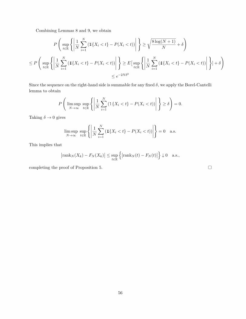
Combining Lemmas 8 and 9, we obtain

P

sup

t2R

(

�

�

�

�

�

1

N

N

X

i=1

( {Xi

< t}� P (X

i

< t))

�

�

�

�

�

)

�r

8 log(N + 1)

N

+ �

!

P

sup

t2R

(

�

�

�

�

�

1

N

N

X

i=1

( {Xi

< t}� P (X

i

< t))

�

�

�

�

�

)

� E

⇥

sup

t2R

(

�

�

�

�

�

1

N

N

X

i=1

( {Xi

< t}� P (X

i

< t))

�

�

�

�

�

)

] + �

!

e

�2N�

2

Since the sequence on the right-hand side is summable for any fixed �, we apply the Borel-Cantellilemma to obtain

P

lim sup

N!1sup

t2R

(

�

�

�

�

�

1

N

N

X

i=1

( {Xi

< t}� P (X

i

< t))

�

�

�

�

�

)

� �

!

= 0.

Taking � ! 0 gives

lim sup

N!1sup

t2R

(

�

�

�

�

�

1

N

N

X

i=1

( {Xi

< t}� P (X

i

< t))

�

�

�

�

�

)

= 0 a.s.

This implies that�

�

rank

N

(X

k

)� F

N

(X

k

)

�

� sup

t2R

n

�

�

rank

N

(t)� F

N

(t)

�

�

o

# 0 a.s.,

completing the proof of Proposition 5.

56

C Empirical Appendix

C.1 Additional Results

Table A1 reports estimates of the e�ect of Grade A o�ers on attrition, computed by estimatingmodels like those used to gauge balance. Under general risk, applicants who receive Grade Aschool o�ers have a slightly higher likelihood of taking the SAT. Decomposing Grade A schoolsinto screened and unscreened schools, applicants who receive unscreened Grade A school o�ersare 1.7 percent more likely to have SAT scores, while o�ers to Grade A screened schools donot correspond to a statistically significant di�erence in the likelihood of having follow-up SATscores. This modest di�erence seems unlikely to bias the 2SLS Grade A estimates reported inTables 4 and 5.

Table A2 reports estimates of the e�ect of enrollment in an ungraded high school. These usemodels like those used to compute the estimates presented in Table 4. OLS estimates show asmall positive e�ect of ungraded school attendance on SAT scores and a strong negative e�ecton graduation outcomes. 2SLS estimates, by contrast, suggest ungraded school attendance isunrelated to these outcomes.

C.2 Bandwidth Computation and Robustness Checks

Bandwidths are estimated as suggested by Imbens and Kalyanaraman (2012), separately for eachscreened program that has applicants on both sides of the cuto�. Bandwidths are estimatedfor the set of applicants who are in the relevant marginal priority group. Bandwidths are alsocomputed separately for each outcome variable. Estimates reported in the text use the smallestof these.

The robustness of this procedure is evaluated by comparing the results generated underalternative restrictions on the distribution of tie-breakers and bandwidth size. Estimates incolumn 2 of Table A3 are from a model that ignores general risk stemming from screenedprograms with four or more duplicate tie-breaker values in the estimated bandwidth, resultingin modest changes in sample and e�ect size. Estimates in column 3 are from a model thatignores general risk stemming from screened programs with any gap of four or more in tie-breaker positions within the estimated bandwidth. Columns 4 and 5 show results that combinethese restrictions, reducing the sample of applicants with general risk by 17 and 31 percent,respectively. The restrictions leave e�ect size and precision largely unchanged.

Table A4 reports 2SLS estimates computed using alternative bandwidths. Halving the band-width size at screened programs reduces the sample of applicants with general risk by about20 percent, while doubling of bandwidth size increases sample size by about 20 percent. Theestimates in column 4 are from regressions that use sixth grade baseline scores instead of SATand graduation outcomes when computing the bandwidth. These variations leave the magnitudeand precision of Grade A school e�ects mostly unchanged.

57

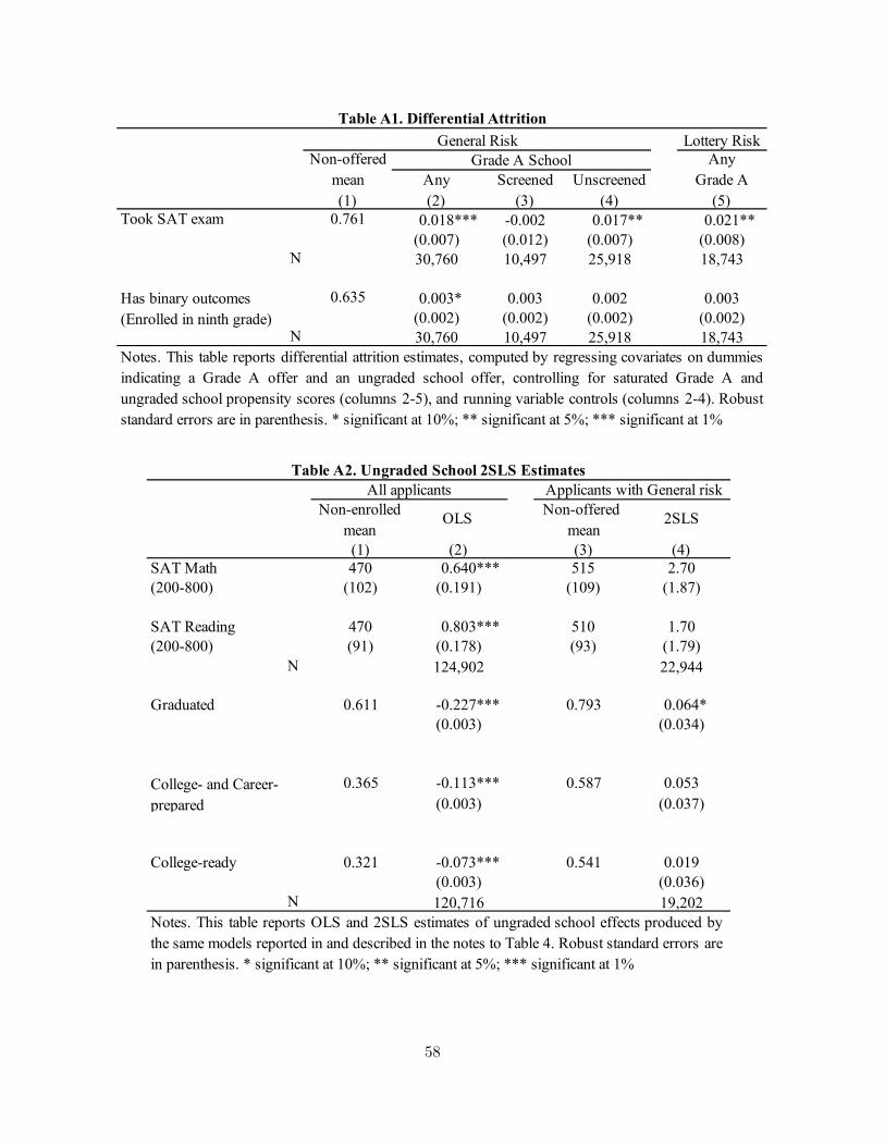
Lottery Risk

Any Screened Unscreened(1) (2) (3) (4) (5)

Took SAT exam 0.761 0.018*** -0.002 0.017** 0.021**(0.007) (0.012) (0.007) (0.008)

N 30,760 10,497 25,918 18,743

0.635 0.003* 0.003 0.002 0.003(0.002) (0.002) (0.002) (0.002)

N 30,760 10,497 25,918 18,743Notes. This table reports differential attrition estimates, computed by regressing covariates on dummiesindicating a Grade A offer and an ungraded school offer, controlling for saturated Grade A andungraded school propensity scores (columns 2-5), and running variable controls (columns 2-4). Robuststandard errors are in parenthesis. * significant at 10%; ** significant at 5%; *** significant at 1%

Table A1. Differential AttritionGeneral Risk

Non-offered mean

Grade A School Any Grade A

Has binary outcomes(Enrolled in ninth grade)

(1) (2) (3) (4) 470 0.640*** 515 2.70

(200-800) (102) (0.191) (109) (1.87)

470 0.803*** 510 1.70(200-800) (91) (0.178) (93) (1.79)

N 124,902 22,944

0.611 -0.227*** 0.793 0.064*(0.003) (0.034)

0.365 -0.113*** 0.587 0.053(0.003) (0.037)

0.321 -0.073*** 0.541 0.019(0.003) (0.036)

N 120,716 19,202

SAT Reading

Table A2. Ungraded School 2SLS EstimatesAll applicants Applicants with General risk

Non-enrolledmean

OLS Non-offered mean

2SLS

SAT Math

Graduated

College- and Career-prepared

College-ready

Notes. This table reports OLS and 2SLS estimates of ungraded school effects produced bythe same models reported in and described in the notes to Table 4. Robust standard errors arein parenthesis. * significant at 10%; ** significant at 5%; *** significant at 1%

58

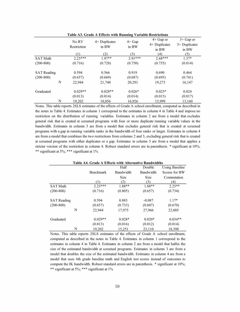
No RV Restriction

4+ Duplicatesin BW

4+ Gapin BW

4+ Gap or 4+ Duplicates

in BW

3+ Gap or 3+ Duplicates

in BW(1) (2) (3) (4) (5)

2.23*** 1.97** 2.91*** 2.68*** 1.37*(200-800) (0.716) (0.728) (0.750) (0.755) (0.814)

0.594 0.566 0.919 0.690 0.464(200-800) (0.657) (0.669) (0.687) (0.695) (0.741)

N 22,944 21,740 20,291 19,273 16,147

0.029** 0.028** 0.026* 0.025* 0.024(0.013) (0.014) (0.014) (0.015) (0.017)

N 19,202 18,056 16,926 15,999 13,160Notes. This table reports 2SLS estimates of the effects of Grade A school enrollment, computed as described in the notes to Table 4. Estimates in column 1 correspond to the estimates in column 4 in Table 4 and impose norestriction on the distribution of running variables. Estimates in column 2 are from a model that excludesgeneral risk that is created at screened programs with four or more duplicate running variable values in thebandwidth. Estimates in column 3 are from a model that excludes general risk that is created at screenedprograms with a gap in running variable ranks in the bandwidth of four ranks or larger. Estimates in column 4are from a model that combines the two restrictions from columns 2 and 3, excluding general risk that is created at screened programs with either duplicates or a gap. Estimates in column 5 are from a model that applies astricter version of the restriction in column 4. Robust standard errors are in parenthesis. * significant at 10%;** significant at 5%; *** significant at 1%

Table A . Grade A Effects with Running Variable Restrictions

SAT Math

SAT Reading

Graduated

BenchmarkHalf

BandwidthSize

DoubleBandwidth

Size

Using Baseline Scores for BW Computation

(1) (2) (3) (4) 2.23*** 1.88** 1.88** 2.25**

(200-800) (0.716) (0.805) (0.657) (0.734)

0.594 0.883 -0.087 1.17*(200-800) (0.657) (0.733) (0.607) (0.670)

N 22,944 17,975 27,966 22,005

0.029** 0.028* 0.020* 0.034**(0.013) (0.016) (0.012) (0.014)

N 19,202 15,251 23,110 18,398Notes. This table reports 2SLS estimates of the effects of Grade A school enrollment,computed as described in the notes to Table 4. Estimates in column 1 correspond to theestimates in column 4 in Table 4. Estimates in column 2 are from a model that halfes thesize of the estimated bandwidth at screened programs. Estimates in column 3 are from amodel that doubles the size of the estimated bandwidth. Estimates in column 4 are from amodel that uses 6th grade baseline math and English test scores instead of outcomes tocompute the IK bandwidth. Robust standard errors are in parenthesis. * significant at 10%;** significant at 5%; *** significant at 1%

Table A . Grade A Effects with Alternative Bandwidths

SAT Math

SAT Reading

Graduated

59