The Real Exchange Rate, Real Interest Rates, and the Risk Premium

Charles Engel University of Wisconsin

cengel@ssc.wisc.edu

October 17, 2012 (First version 5-31-11.)

Abstract

The well-known uncovered interest parity puzzle arises from the empirical regularity that, among developed country pairs, the high interest rate country tends to have high expected returns on its short term bonds. At the same time, another strand of the literature has documented that high real interest rate countries tend to have currencies that are strong in real terms – indeed, stronger than can be accounted for by the path of expected real interest differentials under uncovered interest parity. These two strands – one concerning short-run expected changes and the other concerning the level of the real exchange rate – have apparently contradictory implications for the relationship of the foreign exchange risk premium and interest-rate differentials. This paper documents the puzzle, and shows that it poses a challenge for asset pricing models. The features of a model that might reconcile the findings are discussed.

I thank Bruce Hansen and Ken West for many useful conversations and Mian Zhu and Cheng-Ying Yang for excellent research assistance. I thank David Backus, Gianluca Benigno, Cosmin Ilut, Keyu Jin, Richard Meese, Michael Melvin, Anna Pavlova, John Prins, Alan Taylor, and Adrien Verdelhan for comments on an earlier draft of the paper. I have benefited from helpful comments at seminars at Duke, North Carolina, European Central Bank, Enti Einaudi, International Monetary Fund, Federal Reserve Bank of Phildadelphia, Federal Reserve Bank of Kansas City, Federal Reserve Board, and Wharton. I have benefited from support from the following organizations at which I was a visiting scholar: Federal Reserve Bank of Dallas, Federal Reserve Bank of St. Louis, Federal Reserve Bank of San Francisco, Federal Reserve Board, European Central Bank, Hong Kong Institute for Monetary Research, Central Bank of Chile, and CREI. I acknowledge support from the National Science Foundation grant no. 0451671.

1

This study concerns two prominent empirical findings in international finance that have achieved

almost folkloric status. The interest parity puzzle in foreign exchange markets finds that over short time

horizons (from a week to a quarter) when the interest rate (one country relative to another) is higher than

average, the short-term bonds of the high-interest rate currency tend to earn an excess return. That is, the

high interest rate country tends to have the higher expected return in the short run. A risk-based

explanation of this anomaly requires that the short-term bonds in the high-interest rate country are

relatively riskier, and therefore incorporate an excess return as a reward for risk-bearing.

The second stylized fact concerns evidence that when a country’s relative real interest rate lies

above its average, its currency in levels tends to be stronger than average in real terms. Moreover, the

strength of the currency tends to be greater than is warranted by rational expectations of future short-term

interest differentials. One way to rationalize this finding is to appeal to the influence of expected future

risk premiums on the level of the exchange rate. That is, the country with the relatively high real interest

rate has the lower risk premium and hence the stronger currency. When a country’s real interest rate is

high, its currency is appreciated not only because its bonds pay a higher interest rate but also because they

are less risky.

These two predictions about risk go in opposite directions: the high interest rate country has

higher expected returns in the short run, but a stronger currency in levels. The former implies the high

interest rate currency is riskier, the latter that it is less risky. That is the central puzzle of this paper.

This paper produces evidence in a unified framework that confirms these empirical regularities

for the exchange rates of the G7 countries (Canada, France, Germany, Italy, Japan and the U.K.) relative

to the U.S. However, these findings, taken together, constitute a previously unrecognized puzzle

regarding how cumulative excess returns or foreign exchange risk premiums affect the level of the real

exchange rate. Theoretically, a currency whose assets are perceived to be risky not only currently but

looking forward should be weaker, ceteris paribus. In the data, we find that when the U.S. real interest

rate is high, its short-term bonds are expected to earn a higher return than foreign bonds, but the dollar is

actually stronger in real terms.

It is well-known that macroeconomic models that incorporate the uncovered interest parity

assumption imply short-run behavior of changes in exchange rates that is inconsistent with the empirical

findings of the interest parity puzzle, but it apparently has gone unrecognized that the set of models that

have been built to account for this anomaly are inconsistent with the behavior of the level of the real

exchange rate. Many models of foreign exchange risk premiums predict that the high-interest rate

currency will be weaker than average in real terms and appreciate over both the short- and long-run. On

the other hand, simple models that account for the uncovered interest parity puzzle by positing slow

reaction in asset markets do imply that the high-interest rate currency is strong, but have the implication

2

that the exchange rate is excessively stable (rather than excessively volatile) relative to the interest parity

benchmark. Neither approach is consistent with the observation that the currency is strong, even relative

to the interest-parity milepost, when the country’s real interest rates are high.

The literature on the forward premium anomaly is vast. Classic early references include Bilson

(1981) and Fama (1984). Engel (1996) surveys the early work that establishes this puzzle, and discusses

the problems faced by the literature that tries to account for the regularity. There have been many recent

important contributions, including prominent papers by Backus, Foresi, and Telmer (2002), Lustig and

Verdelhan (2007), Burnside et. al. (2011a, 2011b, 2011c), Verdelhan (2010), Bansal and Shaliastovich

(2012), Backus et. al. (2010).

Dornbusch (1976) and Frankel (1979) are the original papers to draw the link between real

interest rates and the level of the real exchange rate in the modern, asset-market approach to exchange

rates. The connection has not gone unchallenged, principally because the persistence of real exchange

rates and real interest differentials makes it difficult to establish their comovement with a high degree of

uncertainty. For example, Meese and Rogoff (1988) and Edison and Pauls (1993) treat both series as

non-stationary and conclude that evidence in favor of cointegration is weak. However, more recent work

that examines the link between real interest rates and the real exchange rate, such as Engel and West

(2006), Alquist and Chinn (2008), and Mark (2009), has tended to reestablish evidence of the empirical

link. Another approach connects surprise changes in real interest rates to unexpected changes in the real

exchange rate. There appears to be a strong link of the real exchange rate to news that alters the expected

real interest differential – see, for example, Faust et. al. (2006), Andersen et. al. (2007) and Clarida and

Waldman (2008).

However, it is widely recognized that exchange rates are excessively volatile relative to the

predictions of monetary models that assume interest parity, or no foreign exchange risk premium.

Frankel and Meese (1987) and Rogoff (1996) are prominent papers that make this point. Evans (2011)

refers to the “exchange-rate volatility puzzle” as one of six major empirical challenges in the study of

exchange rates. Recent contributions include Engel and West (2004), Bacchetta and van Wincoop

(2006), and Evans (2012).

The study of risk premiums in foreign exchange markets sheds light on important questions in

asset pricing that go beyond the narrow interest of specialists in international asset markets. The foreign

exchange rate is one of the few, if not the only, aggregate asset for an economy whose price is readily

measurable, so its pricing offers an opportunity to investigate some key predictions of asset pricing

theories. For example, in the absence of arbitrage, the rate of real depreciation of the “Home” country’s

currency equals the log of the stochastic discount factor (s.d.f.) for Foreign returns relative to the log of

the corresponding s.d.f. for Home returns, while the risk premium (as conventionally measured) is

3

proportional to the conditional variance of the log of the s.d.f. for Home relative to the variance of the

s.d.f. for Foreign returns.1 Thus, the behavior of the foreign exchange rate gives direct evidence on the

fundamental building blocks of equilibrium asset pricing models.

Section 1 develops the approach of this paper. Section 2 presents empirical results. Section 3

explains why the empirical findings constitute a puzzle. It develops some general conditions that have to

be satisfied in order to account for our empirical findings, and then shows that existing theories do not

satisfy these conditions. We discuss the difficulties encountered by asset pricing approaches such as

representative agent models of the risk premium, and models of “delayed overshooting”.2 We then

describe the features of a model that can reconcile the empirical findings. In section 4, we consider

various caveats to our findings.

1. Excess Returns and Real Exchange Rates

We develop here a framework for examining behavior of ex ante excess returns and the level of

the real exchange rate. Our set-up will consider a Home and Foreign country. In the empirical work of

section 2, we always take the US as the Home country (as does the majority of the literature), and

consider other major economies as the Foreign country. Let ti be the one-period nominal interest in

Home. We denote Foreign variables throughout with a superscript *, so *ti is the Foreign interest rate. ts

denotes the log of the foreign exchange rate, expressed as the US dollar price of Foreign currency. 1t tE s

refers to the expectation, conditional on time t information, of the log of the spot exchange rate at time

1t . We define the “expected excess return”, t , as:

(1) *1t t t t t ti E s s i .

This definition of expected returns corresponds with the definition in the literature. We can

interpret *1t t t ti E s s as a first-order log approximation of the expected return in Home currency terms

for a Foreign security. As Engel (1996) notes, the first-order log approximation may not really be

adequate for appreciating the implications of economic theories of the excess return. For example, if the

exchange rate is conditionally log normally distributed, then 11 1 12ln ( / ) var ( )t t t t t t t tE S S E s s s ,

where 1var ( )t ts refers to the conditional variance of the log of the exchange rate. Engel (1996) points

out that this second-order term is approximately the same order of magnitude as the risk premiums

1 The s.d.f.s for Home and Foreign returns are unique only when asset markets are complete. See Backus et. al. (2002), Brandt et. al. (2006), and section 3.2 below. 2 “Representative agent models” may be an inadequate label for models of the risk premium that are developed off of the Euler equation of a representative agent under complete markets, generally taking the consumption stream as exogenous. “Delayed overshooting” refers to models in which agents are not necessarily able to rebalance their portfolios instantly in response to shocks.

4

implied by some economic models. However, we proceed with analysis of t defined according to

equation (1) both because it is the object of almost all of the empirical analysis of excess returns in

foreign exchange markets, and because the theoretical literature that we consider in section 3 seeks to

explain t as defined above including possible movements in 1var ( )t ts .

The well-known uncovered interest parity puzzle comes from the empirical finding that the

change in the log of the exchange rate is negatively correlated with the Home less Foreign interest

differential, *t ti i . That is, estimates of * *

1 1cov( , ) cov( , )t t t t t t t t ts s i i E s s i i tend to be negative.

As Engel (1996) surveys, and subsequent empirical work confirms, this finding is consistent over time

among pairs of high-income, low-inflation countries.3 From equation (1), we note that the relationship *

1cov( , ) 0t t t t tE s s i i is equivalent to * *cov( , ) var( ) 0t t t t ti i i i . That is, when the Home

interest rate is relatively high, so *t ti i is above average, the excess return on Home assets also tends to

be above average: t is below average. This is considered a puzzle because it has been very difficult to

find plausible economic models that can account for this relationship.

Let tp denote the log of the consumer price index at Home, and 1 1t t tp p is the inflation

rate. The log of the real exchange rate is defined as *t t t tq s p p . The ex ante real one-period real

interest rates, Home and Foreign, are given by 1t t t tr i E and * * *1t t t tr i E . Note also

*1 1 1 1t t t t t t t t t tE q q E s s E E . We can rewrite (1) as:

(2) *1t t t t t tr r E q q .

We take as uncontroversial the proposition that the real interest differential, *t tr r , and expected excess

returns, t , are stationary random variables without time trends, and denote their means as r and ,

respectively. We will also stipulate that there is no deterministic time trend or drift in the log of real

exchange rates, so that the unconditional mean of 1t t tE q q is zero. Rewriting (2):

(3) *1 ( ) ( )t t t t t tq E q r r r .

Iterate equation (3) forward, applying the law of iterated expectations, to get:

(4) limt t t j t tjq E q R ,

where

(5) *

0

( )t t t j t jj

R E r r r , and

3 Bansal and Dahlquist (2000) find that the relationship is not as consistent among emerging market countries, especially those with high inflation.

5

(6) 0

( )t t t jj

E .

tR is the expected sum of the current and all future values of the Home less Foreign real interest

differential (relative to its unconditional mean). It is important to note that tR is not the real interest

differential on long-term bonds, even hypothetical infinite-horizon bonds. tR is the difference between

the expected real return from holding an infinite sequence of short-term Home bonds and the expected

real return from the infinite sequence of short-term Foreign bonds. An investment that involves rolling

over short term assets has different risk characteristics than holding a long-term asset, which might

include a holding-period risk premium.

Similarly, t is the expected infinite sum of excess returns on the Foreign security. We label this

the ex ante “level excess return” or “level risk premium”, to make reference to its influence on the level of

the real exchange rate.

The left-hand side of (4), limt t t jjq E q , can be interpreted as the transitory component of the

real exchange rate. In fact, according to our empirical findings reported in section 2, we can treat the real

exchange rate as a stationary variable, so lim t t jjE q q . As is well known, even if the real exchange

rate is stationary, it is very persistent. Engel (2000), in fact, argues that it may be practically impossible

to distinguish between the stationary case and the unit root case under plausible economic conditions. We

proceed in examining tq q , assuming stationarity, but note that our methods could be applied to the

transitory component of the real exchange rate, taken as the difference between tq and a measure of the

permanent component, lim t t jjE q . In section 4, we note how Engel’s (2000) interpretation implies that

in practice it may not be possible to distinguish a permanent and transitory component, but make the case

that the economic analysis of that paper argues for treating the real exchange rate as stationary.

In section 3, we discuss the common assumption in theoretical models of expected returns that

markets are complete, implying that log of the real exchange rate change is equal to the difference

between the logs of the marginal utilities of a Home consumer and Foreign consumer (plus a constant).

Stationarity of the real exchange rate is completely compatible with a unit root in the log of consumption,

or in the marginal utility of consumption. It requires simply that Home and Foreign marginal utilities of

consumption be cointegrated, which is a natural condition among well-integrated economies such as the

highly developed countries used in this study. It is analogous to the assumption made in almost all

closed-economy models that we can treat the marginal utilities of different consumers within a country as

cointegrated.

6

Under the stationarity assumption, we can write (4) as:

(7) IPt t tq q , IP

t tq R q .

The level excess return, t , captures the potential effect of risk premiums on the level of the real

exchange rate, holding tR constant. We use the notation IPtq to denote the “interest parity” level of the

real exchange rate, or the value of tq setting 0t .

In the next section, we present evidence that *cov( , ) 0IPt t tq r r and *cov( , ) 0t t tr r . Taken

together, these two findings imply from (7) that *cov( , ) 0t t tq r r , which jibes with the concept familiar

from Dornbusch (1976) and Frankel (1979) that when a country’s real interest rate is high (relative to the

foreign real interest rate, relative to average), its currency tends to be strong in real terms (relative to

average.) But if *cov( , ) 0t t tr r , the strength of the currency cannot be attributed entirely to IPtq , as it

would be in Dornbusch and Frankel (who both assume uncovered interest parity, or that 0t .) The

relationship between expected excess returns and real interest differential plays a role in determining the

relation between the real exchange rate and real interest rates.

It is entirely unsurprising that we find *cov( , ) 0IPt t tq r r . This simply implies that there is not a

great deal of non-monotonicity in the adjustment of real interest rates toward the long run mean.

The central puzzle raised by this paper concerns the two findings, *cov( , ) 0t t tr r and

*cov( , ) 0t t tr r . The short-run ex ante excess return on the Foreign security, t , is negatively

correlated with the real interest differential, consistent with the many empirical papers on the uncovered

interest parity puzzle. But the level excess return, t , is positively correlated. Given the definition of t

in equation (6), we must have that for at least 0j and possibly for some 0j , *cov( , ) 0t t j t tE r r ,

but for other 0j , *cov( , ) 0t t j t tE r r . The sum of the latter covariances must exceed the sum of the

former to generate *cov( , ) 0t t tr r . As we discuss in section 3, models in the literature that are

constructed to account for *cov( , ) 0t t tr r , have the counterfactual implication that *cov( , ) 0t t tr r .

The empirical approach of this paper can be described simply. We estimate VARs in the

variables tq , *t ti i , and * *

1 1 ( )t t t ti i . From the VAR estimates, we construct measures of

* * *1 1( )t t t t t t tE i i r r . Using standard projection formulas, we can also construct estimates of

IPtq . To measure t , we take the difference of IP

tq and tq . From these VAR estimates, we calculate our

estimates of the covariances just discussed. As an alternative approach, we estimate VARs in tq , *t ti i ,

7

and *t t , and then construct the needed estimates of *

t tr r , IPtq , and t .4 The estimated covariances

under this alternative approach are very similar to those from the original VAR. Our approach of

estimating undiscounted expected present values of interest rates from VARs is presaged in Mark (2009)

and Brunnermeier et. al. (2009).5

2. Empirical Results

We investigate the behavior of real exchange rates and interest rates for the U.S. relative to the

other six countries of the G7: Canada, France, Germany, Italy, Japan, and the U.K. We also consider the

behavior of U.S. variables relative to an aggregate weighted average of the variables from these six

countries.6 Our study uses monthly data. Foreign exchange rates are noon buying rates in New York, on

the last trading day of each month, culled from the daily data reported in the Federal Reserve historical

database. The price levels are consumer price indexes from the Main Economic Indicators on the OECD

database. Nominal interest rates are taken from the last trading day of the month, and are the midpoint of

bid and offer rates for one-month Eurorates, as reported on Intercapital from Datastream. The interest

rate data begin in June 1979. Most of our empirical work uses the time period June 1979 to October

2009. In some of the tests for a unit root in real exchange rates, reported in the Appendix, we use a longer

time span from June 1973 to October 2009. It is important for our purposes to include these data well

into 2009 because it has been noted in some recent papers that there was a crash in the “carry trade” in

2008, so it would perhaps bias our findings if our sample ended prior to this crash.7 We treat the real

exchange rates as stationary throughout our empirical analysis.

The Appendix details evidence that allows us to reject a unit root in real exchange rates. It is well

known that real exchange rates among advanced countries are very persistent.8 There is no consensus on

whether these real exchange rates are stationary or have a unit root. Two recent studies of uncovered

interest parity, Mark (2010) and Brunnermeier, et. al. (2009) estimate statistical models that assume the

real exchange rate is stationary, but do not test for a unit root. Jordà and Taylor (2012) demonstrate that

there is a profitable carry-trade strategy that exploits the uncovered interest parity puzzle when the trading

rule is enhanced by including a forecast that the real exchange rate will return to its long-run level when

its deviations from the mean are large. That paper assumes a stationary real exchange rate and includes 4 We also consider VARs that are augmented with data on stock market returns and long-term interest rates, which are included solely for the purpose of improving the forecasts of future interest rates and inflation rates. 5 This method does not require estimation of long-term real interest rates, about which there is some controversy, but instead estimates the sum of expected future short term nominal interest rates less expected inflation. See Bansal, et. al. (2012). 6 The weights are determined by the value of each country’s exports and imports as a fraction of the average value of trade over the six countries. 7 See, for example, Brunnermeier, et. al. (2009) and Jordà and Taylor (2012). 8 See Rogoff (1996) for example.

8

statistical tests that cannot reject cointegration of ts with *t tp p .

2.1 Fama regressions

The “Fama regression” (see Fama, 1984) is the basis for the forward premium puzzle. It is

usually reported as a regression of the change in the log of the exchange rate between time t+1 and t on

the time t interest differential:

*1 , 1( )t t s s t t s ts s i i u

Under uncovered interest parity, 0s and 1s . We can rewrite this regression as:

(8) * *1 , 1( )t t t t s s t t s ti s s i i i u ,

where 1s s . The left-hand side of the regression is the ex post excess return on the Foreign

security. If 0s but 0s , then the high-interest rate currency tends to have a higher excess return.

There is a positive correlation between the excess return on the Foreign currency and the Foreign-Home

interest differential.

Table 1 reports the 90% confidence interval for the regression coefficients from (8), based on

Newey-West standard errors. For all of the currencies, the point estimates of s are positive. The 90%

confidence interval for s lies above zero for four (Italy and France being the exceptions, where the

confidence interval for the latter barely includes zero.) For four of the six, zero is inside the 90%

confidence interval for the intercept term, s . (In the case of the U.K., the confidence interval barely

excludes zero, while for Japan we find strong evidence that s is greater than zero.)

The G6 exchange rate (the weighted average exchange rate, defined in the data section) appears

to be less noisy than the individual exchange rates. In all of our tests, the standard errors of the

coefficient estimates are smaller for the G6 exchange rate than for the individual country exchange rates,

suggesting that some idiosyncratic movements in country exchange rates get smoothed out when we look

at averages. The weights in the G6 exchange rate are constant. We can think of this exchange rate as the

dollar price of a fixed basket of currencies, and can interpret our tests as examining the properties of

expected returns on this asset. Our discussion focuses on the returns on this asset because its returns

appear to be more predictable than for the individual currencies. Examining the behavior of the returns

on the weighted portfolio is a more appealing way of aggregating the data and reducing the effects of the

idiosyncratic noise in the country data than estimating the Fama regression as a panel using all six

exchange rates. There is not a good theoretical reason to believe that the coefficients in the Fama

regression are the same across currencies, so the gains from panel methods are likely to be small because

the panel would impose no restrictions across the equations on the coefficients. Table 1 reports that the

9

90% confidence interval for this exchange rate lies well above zero, with a point estimate of 2.467.9

2.2 Fama regressions in real terms

Regression (8) in real terms can be written as:

(9) 1 , 1ˆ ˆd dt t t q q t q tq q r r u .

In this regression, ˆdtr refers to estimates of the ex ante real interest rate differential,

* *1 1( )d

t t t t t t tr i E i E . We estimate the real interest rate from VARs. As noted above, we

consider two different VAR models. Model 1 is a VAR with 3 lags in the variables tq , *t ti i , and

* *1 1 ( )t t t ti i . From the VAR estimates, we construct measures of d

tr . Model 2 is a 3-lag VAR in

tq , *t ti i , and *

t t .

There are two senses in which our measures of ˆdtr are estimates. The first is that the parameters

of the VAR are estimated. But even if the parameters were known with certainty, we would still only

have estimates of dtr because we are basing our measures of d

tr on linear projections. Agents certainly

have more sophisticated methods of calculating expectations, and use more information than is contained

in our VAR.

The findings regression (9) in real terms are similar to those when the regression is estimated on

nominal variables. For all currencies, the estimates of q , reported in Table 2, are positive, which

implies that the high real interest rate currency tends to have high real expected excess returns. The

estimated coefficient for the G6 aggregate is close to 2. This summary is true for both VAR models.

Table 2 and all of the subsequent tables report three sets of confidence intervals for each

parameter estimate. The first is based on Newey-West standard errors, ignoring the fact that ˆdtr is a

generated regressor. The second two are based on bootstraps. The first bootstrap uses percentile intervals

and the second percentile-t intervals.10

From Table 2, all three sets of confidence intervals are similar. For the individual currencies, for

both Model 1 and Model 2, the confidence interval for q lies above zero for Germany, Japan, and the

U.K. It contains zero for Canada and Italy, and contains zero for France except using the second

confidence interval. The point estimates from the Fama regressions in nominal returns (reported in Table

1) and in real terms (Table 2) are quite similar, but the confidence intervals for the bilateral exchange

rates are wider, leading to fewer rejections of the uncovered interest parity null.

9 The intercept coefficient, on the other hand is very near zero, and the 90% confidence interval easily contains zero. 10 See Hansen (2010). The Appendix describes the bootstraps in more detail.

10

The findings are clear using the G6 average exchange rate: the coefficient estimate is 1.93 when

the real interest estimate comes from Model 1, and 1.91 when Model 2 is used. All of the confidence

intervals lie above zero. For both models, the estimate of q is very close to zero, and the confidence

intervals contain zero.

In summary, the evidence on the interest parity puzzle is similar in real terms as in nominal terms.

The point estimates of the coefficient q are positive and tend to be statistically significantly greater than

zero, which implies cov( , ) 0dt tr . Even in real terms, the country with the higher interest rate tends to

have short-run excess returns (i.e., excess returns and the interest rate differential are positively

correlated.)

2.3 The real exchange rate, real interest rates, and the level risk premium

Table 3 reports estimates from

(10) ,ˆdt q Q t q tq r u .

In all cases (all currencies, for both Model 1 and Model 2), the coefficient estimate is negative. In almost

all cases, although the confidence intervals are wide, the coefficient is significantly negative.11

Recall from equation (7) that IPt t tq q , where IP

t tq R q . If there were no excess returns,

so that IPt tq q , and d

tr were positively correlated with tR , then there is a negative correlation between

tq and dtr . That is, under uncovered interest parity, the high real interest rate currency tends to be

stronger. For example, this is the implication of the Dornbusch-Frankel theory in which real interest

differentials are determined in a sticky-price monetary model.

But we can make a stronger statement – there is a relationship between the real interest

differential, ˆdtr , and our measure of the level excess return, ˆ

t (where ˆt is our estimate of t based on

the VAR models.) Our central empirical finding is reported in Table 4. This table reports the regression:

(11) ˆ ˆdt t tr u .12

In all cases, the estimated slope coefficient is positive, implying cov( , ) 0dt tr . The 90 percent

confidence intervals are wide, but with a few exceptions, lie above zero. The confidence interval for the

G6 average strongly excludes zero. To get an idea of magnitudes, a one percentage point difference in

11 The exceptions are that the third confidence interval contains zero for Model 1 for France, and Models 1 and 2 for the U.K. 12 To be precise, ˆ

t is calculated as the difference between tq and our VAR estimate of tR . To calculate our estimate of tR , given by the infinite sum of equation (5), we demean *

t j t jr r by its sample mean. We use the sample mean rather than maximum likelihood estimate of the mean because it tends to be a more robust estimate.

11

annual rates between the home and foreign real interest rates equals a 1/12th percentage point difference in

monthly rates. The coefficient of around 32 reported for the regression when we take the U.S. relative to

the average of the other G7 countries translates into around a 2.7% effect on the level risk premium. That

is, if the U.S. real rate increases one annualized percentage point above the real rate in the other countries,

the dollar is predicted to be 2.7% stronger in real terms from the level risk premium effect.

This finding that cov( , ) 0dt tr is surprising in light of the well-known uncovered interest parity

puzzle. In the previous two subsections, we have documented that when dtr is above average, Home

bonds tend to have expected excess returns relative to Foreign bonds. That seems to imply that the high

interest rate currency is the riskier currency. But the estimates from equation (11) deliver the opposite

message – the high interest rate currency has the lower level risk premium. t is the level risk premium

for the Foreign currency – it is positively correlated with dtr , so it tends to be high when d

tr is high.

We can write

(12) 0

cov( , ) cov[ ( ), ]t t tj

t td

jdr rE .

The short-run interest parity puzzle establishes that cov( , ) 0td

tr . Clearly if cov( , ) 0td

tr , then we

must have cov[ ( ), ] 0t t jd

tE r for at least some 0j . That is, in order for cov( , ) 0td

tr , we must

have a reversal in the correlation of the short-run risk premiums with dtr as the horizon extends.

This is illustrated in Figure 2, which plots estimates of the slope coefficient in a regression of

1ˆ ( )t t jE on ˆd

tr for 1, ,100j :

1 ,ˆ ( ) ˆd j

jt t j tj tr uE

For the first few j, this coefficient is negative, but it eventually turns positive at longer horizons.

The Figure also plots the slope of regressions of 1ˆ ( )d

t t jE r on ˆdtr for 1, ,100j :

*1 1 ,

ˆ ˆ( ) d jt t j t j rj rj t r tE r r r u

These tend to be positive at all horizons.

The Figure also includes a plot of the slope coefficients from regressing 1ˆ ( )t t j t jE q q for

1, ,100j :

1 ,ˆ ˆ( ) d j

t t j t j qj qj t q tE q q r u

Since 11 1ˆˆ ( (ˆ) )d

t t j t j t j t t jtE q q E r E , these regression coefficients are simply the sum of the other

two regression coefficients that are plotted. In this case, the regression coefficients start out negative for

12

the first few months, but then turn positive for longer horizons.

To summarize, when the Home real interest rate relative to the Foreign real interest rate is higher

than average, the Home currency is stronger in real terms than average. Crucially, it is even stronger than

would be predicted by a model of uncovered interest parity. Ex ante excess returns or the foreign

exchange risk premium contribute to this strength. If Home’s real interest rate is high – in the sense that

the Home relative to Foreign real interest rate is higher than average – the level risk premium on the

Foreign security is higher than average.

Figure 2 presents a slightly different perspective. This chart plots the slope coefficients from

regressions of IPt jq and t jq on ˆd

tr for the G6 average exchange rate.13 That is, it plots the estimated

slope coefficients from the regressions:

,ˆ ˆIP d jt j Rj Rj t R tq r u

,ˆd jt j Qj Qj t Q tq r u .

If interest parity held, the behavior of the real exchange rate should conform to the plot for IPt jq .

That line indicates that the U.S. dollar tends to be strong in real terms when ˆdtr is high, and then is

expected to depreciate back toward its long-run mean. The line for the regression of t jq on ˆdtr shows

three things: First, when ˆdtr is above average, the dollar tends to be strong in real terms, and much

stronger than would be implied under uncovered interest parity. Second, when ˆdtr is above average, the

dollar is expected to appreciate even more in the short run. This is the uncovered interest parity puzzle.

Third, when ˆdtr is above average, the dollar is expected to reach its maximum appreciation after around 5

months, then to depreciate gradually.14 One implication of these dynamics is similar to Jordà and

Taylor’s (2012) findings about forecasting nominal exchange rate changes. They find that the nominal

interest differential can help to predict exchange rate changes in the short run: the high interest rate

currency is expected to appreciate (contrary to the predictions of uncovered interest parity.) But the

forecasts of the exchange rate can be enhanced by taking into account purchasing power parity

considerations. The deviation from PPP helps predict movements of the nominal exchange rate as the

real exchange rate adjusts toward its long-run level.

We consider two extensions of the empirical analysis to see if augmenting the simple VARs

estimated here can sharpen the forecasts of future short-term real interest rates. The results reported so far

are from VARs with three lags, using monthly data. We estimated the model using 12 lags for all VARs.

13 The plots for most of the other real exchange rates look qualitatively very similar. 14 The line labeled “Model” is discussed in the next section.

13

The second extension added two variables to the VARs for each country – a stock price index and a

measure of long-term nominal government bond yields. The long-term bond yields are from the IMF’s

International Financial Statistics, “interest rates, government securities and government bonds.” The

stock price indexes are monthly, from Datastream.15 These augmented VARs were then used to construct

regressions of the form reported in Tables 2, 3, and 4.

The point estimates from the augmented models were quite similar to those from the more

parsimonious models, but the confidence intervals were wider. In short, the augmented models do not

seem to add any useful information. Figure 3 reproduces the plot of the slope coefficient estimates that

correspond to Figure 2. The top panel is for the 12-lag VAR, and the bottom for the VAR augmented

with stock-price and government bond yield data.

We turn now to the implications of these empirical findings for models of the foreign exchange

risk premium.

3. The Puzzle

3.1 The General Problem

Macroeconomic models that are built to explain the uncovered interest parity often incorporate

only a single macroeconomic variable that drives both interest rates and ex ante excess returns. Write the

moving average representations of dtr and t as:

(13) 0

dt j t j

jr a

0t j t j

jc ,

where t is a zero mean, unit variance, i.i.d. random variable.16

There are two common formulations of such models. In the first, there is a common factor that

drives both dtr and t . In a linear model, d

tr and t are linear functions of the factor, so dt tr k for

some constant k. In this case, there may not be any restrictions on the pattern of signs (positive or

negative) for ja and jc . The second typical set-up assumes the impulse response functions for dtr and

t do not change signs as j increases (so ja and jc do not change signs), but does not necessarily require

that dt tr k .

In the first case, cov( , ) var( )dt t tr k , so the finding that cov( , ) 0d

t tr requires 0k .

Since dt tr k , then IP

t tq k and cov( , ) cov( , )d IP dt t t tr k q r . The data show, and many models

15 The Datastream codes are TOTMKCN(PI), TOTMKFR(PI), TOTMKIT(PI), TOTMKUK(PI), TOTMKBD(PI), TOTMKJP(PI), and TOTMKUS(PI) 16 For convenience, constant terms are dropped in the rest of section 3.

14

assume strong positive serial correlation in the real interest differential, so cov( , ) 0IP dt tq r . With 0k ,

this implies cov( , ) 0dt tr , in contradiction to the data.

This type of model implies 1 (1 )d dt t t t tE d r k r , (we adopt the notation 1 1t t td q q for

the real rate of depreciation.) Such a model implies that dtr incorporates all of the relevant information

required to forecast 1td . It is common to calibrate models so that 1 0k , to match the negative

correlation of the depreciation rate with the interest differential. Since (1 )IPt t t tq q k , and we

have seen this class of models implies cov( , ) 0dt tr then the models also predict the real exchange rate

level is positively correlated with dtr , cov( , ) 0d

t tq r . Figure 1 illustrates the problem. As already

noted, this chart plots the slope coefficients from regressions of IPtq and t jq on d

tr for the G6 average

exchange rate – these are the lines labeled bRj and bQj, respectively. The third line, labeled Model, is an

example of the theoretical regression coefficients of lim t t kkt jq E q on dtr implied by the models that

assume perfect correlation between the interest differential and the risk premium, which are discussed

below in section 3.2. The models are built to account for the empirical finding that the Home currency

tends to appreciate in the short run when the home interest rate is high, but the models leave the

correlation of the level of the real exchange rate and the real interest differential with the wrong sign. 17

The second type of model is the one that assumes the impulse response functions of dtr and t do

not change signs. To account for the finding that cov( , ) 0dt tr , and normalizing 0ja , j , we must

assume 0jc , j because 0

cov( , ) jd

t t jj

a cr . This assumption implies 0

cov( , ) 0dt t j i

j i jr a c ,

in contradiction to our empirical findings.

In order to have cov( , ) 0dt tr and cov( , ) 0d

t tr , there must be at least two different variables

driving dtr and t , if we assume that the impulse response functions to each shock do not change signs:

(14) 1 1, 2 2,0 0

dt j t j j t j

j jr a a 1 1, 2 2,

0 0t j t j j t j

j jc c ,

where 1t and 2t are white noise shocks. Two sources of shocks are necessary but not sufficient. It

must be the case that 1 ja and 1 jc are opposite signs, while 2 ja and 2 jc are the same sign.18 dtr and t

must respond in opposite directions to one of the shocks to explain the interest parity puzzle, but in the

17 In terms of Figure 2, it is the fact that the Model line and the solid line for the actual real exchange rate are both initially downward sloping that demonstrates the models can account for 1cov( , )d

t t tE d r in the data. 18 Or vice-versa.

15

same direction to account for the covariance of the interest differential and t . Typically a model that

introduces more than one source of risk does not resolve the puzzle, since, as we see in section 3.2, the

response of dtr and t to the two sources of risk are qualitatively the same.

3.2 Models of the foreign exchange risk premium under complete markets

Almost since the initial discovery of the interest-parity puzzle, there have been attempts to

account for the behavior of expected returns in foreign exchange markets without relying on any market

imperfections, such as market incompleteness or deviations from rational expectations.19 The literature

has built models of risk premiums based on risk aversion of a representative agent. Those models

formulate preferences in order to generate volatile risk premiums which are important not only for

understanding the uncovered interest parity puzzle, but also a number of other puzzles in asset pricing

regarding returns on equities and the term structure.20 Here we briefly review the basic theory of foreign exchange risk premiums in complete-markets

models and relate the factors driving the risk premium to the state variables driving stochastic discount

factors. See, for example, Backus et. al. (2001) or Brandt et. al. (2006).

When markets are complete, there is a unique stochastic discount factor, 1tM that prices returns

denominated in units of the Home consumption basket. That is, the returns on any asset j denominated in

units of Home consumption satisfy , 111 ( )j tr

t tE M e for all j. Likewise, there is a unique s.d.f., *1tM that

prices returns expressed in units of the Foreign consumption basket. As Backus et. al. (2001) show, when

the s.d.f. and returns are log-normally distributed (or, as an approximation), we can write:

(15) *1 1 1t t t t t tE d E m E m ,

(16) *11 12 (var var )t t t t tm m

(17) * *11 1 1 12( ) (var ( ) var ( ))d

t t t t t t t tr E m m m m

The lower case variables, 1tm and *1tm are the logs of 1tM and *

1tM , respectively.

It is convenient to discuss the literature that builds general equilibrium economic models based

with complete markets, based on optimizing behavior by households, in the context of the affine pricing

models of Backus et. al. (2001). The models we examine express 1tm and *1tm , as linear functions of

state variables itz (ignoring intercepts):

(18) 1/ 21 1

1 1( )

k k

t i it i i i it iti i

m z z

19 See Engel (1996) for a survey of the earlier theoretical literature. 20 See for example Bansal and Yaron (2004).

16

(19) * * * * * 1/ 2 *1 1

1 1( )

k k

t i it i i i it iti i

m z z

We assume it and *it are i.i.d. over time, with mean zero and variance equal to one. The it are

mutually independent as are the *it , but it and *

it could be correlated for each i. We assume the state

variables follow the processes (again, setting unconditional means to zero for convenience):

(20) 1 1it i it itz z ,

where 0 1i , and it are i.i.d. over time with mean zero and variance equal to one. 21 Equations (18)-

(20) are a special case of the general formulation in Backus et. al. (2001), but encompass all of the models

we subsequently discuss. This formulation allows for independent factors to influence 1tm and *1tm

because some of the parameters ( i , *i , i ,

*i , i , *

i ) may be zero.

From these equations, ignoring the intercept terms, we have:

(21) * *

1( )

kd

t i i i i iti

r z , 212i i i , * *2 *1

2i i i

(22) *

1( )

k

t i i iti

z

As noted above, in order to build a model that can account for both cov( , ) 0dt tr and

cov( , ) 0dt tr , we need at least two factors driving 1t tE d and t .22 The models in the literature fall

into two categories, symmetric and asymmetric.

Consider symmetric models with driving variables labeled 1tz , 2tz , *1tz , and *

2tz . For example,

consumption growth in each country may have a permanent and a transitory component. 1tz and *1tz may

be the variances of the permanent components in Home and Foreign, respectively, and 2tz and *2tz may

be the variances of the transitory components. In this class of symmetric models, the preference

parameters of households are the same in Home and Foreign, and the parameters of the stochastic

processes for itz and *itz , 1,2i are the same for each i. Ignoring constant terms, we can specialize (21)

and (22) in this case to be:23

(23) * *1 1 1 1 2 2 2 2( )( ) ( )( )d

t t t t tr z z z z

21 We follow the literature and assume that when itz is negative, we still have i i itz positive, and likewise in the Foreign country. 22 In fact, the conditions in the appendix are necessary and sufficient for a multi-factor model. There must be a grouping of factors into two groups, which satisfy the conditions. 23 In other words, *

1tz maps into 3tz in equations (18) and (19), and *2tz maps into 4tz . Then, e.g., *

1 0 , *2 0 ,

3 0 , 4 0 , *3 1 and *

4 2 .

17

(24) * *1 1 1 2 2 2( ) ( )t t t t tz z z z .

There are two factors, *1 1t tz z and *

2 2t tz z , each AR(1) processes with persistence i , 1,2i ,

that drive dtr and t , so this formulation is a special case of (14). To account for the empirical findings

of cov( , ) 0dt tr and cov( , ) 0d

t tr , the response of dtr and t to the two factors must be in opposite

directions. Normalize 1 2, 0 , so an increase in each of the factors raises t . Then to explain the

empirical facts, we need at least that 1 10 and 2 2 0 .24

Models with complete markets and rational expectations, but with standard preferences (based on

expected utility, time-separable preferences) are unsuccessful in accounting for the interest parity puzzle,

as Bekaert et. al. (1997) show. That paper argues that only models with non-standard preferences have

the potential for explaining the interest-parity puzzle. Backus et. al. (2001) further delineate a set of

restrictions that must hold on linear representations of the log of the stochastic discount factor that will be

consistent with complete-markets, risk premium explanations for the interest parity puzzle.

Verdelhan (2010) builds a two-country endowment model, with a representative agent in each

country whose preferences are of the form first proposed by Campbell and Cochrane (1999).25 Bansal

and Shaliastovich (2012) consider models in which households have Epstein-Zin (1989) preferences.26 It

is immediate that neither of these approaches can successfully explain both cov( , ) 0dt tr and

cov( , ) 0dt tr because in both cases, a single factor drives expected returns and the risk premium. We

have already seen that no single-factor model will work.

In Verdelhan’s approach based on Campbell-Cochrane preferences, the single factor is related to

the consumption “habit” in each country. Each agents utility depends on his consumption relative to tH ,

an aggregate “habit” level that is determined as a function of the aggregate consumption level. Then

define in Verdelhan’s notation t tt

t

C HSC

, where tC is the aggregate per capita consumption. An

analogous expression defines *tS . tS is determined by a stochastic processes that relates it to its own lag

and shocks to consumption growth, which itself is exogenously specified (and analogously for *tS .) The

single factor that drives expected returns and risk premiums is *(log( ) log( ))t tS S .

Bansal and Shaliastovich (2012) extend Bansal and Yaron’s (2004) “long-run risks” model to the

24 Or the opposite. 25 Moore and Roche (2010) also use Campbell-Cochrane preferences to provide a solution to the interest parity puzzle. 26 Bekaert et. al. (1997) and Lustig and Verdelhan (2007) are earlier approaches that also use Epstein-Zin preferences.

18

open economy.27 The single factor that drives expected returns and the risk premium is the difference

between the variances of the long-term growth rates of consumption in the Home and Foreign economies.

It is difficult to conceive of a natural generalization of the symmetric model with Campbell-

Cochrane preferences to two factors, since that would imply there are two habit levels that matter for

utility. The symmetric long-run risk model, on the other hand, could be generalized because there might

be different components to consumption growth, whose variance could affect both expected returns and

the risk premium. However, the restrictions on preferences that can deliver the result that cov( , ) 0dt tr

will also imply cov( , ) 0dt tr . Following Lustig, et. al. (2011), the economic intuition of these

restrictions comes from the fact that in order to explain the interest parity puzzle, there must be factors

that drive both 1var ( )t tm and 1( )t tE m (and similarly in the foreign country.) i measures the impact of

an increase in factor i on the volatility of the s.d.f. If the increase in risk lowers interest rates, then

0 i i . As Lustig et. al. explain: “This condition is intuitive and has a natural counterpart in most

consumption-based asset pricing models: when precautionary saving demand is strong enough, an

increase in the volatility of … marginal utility growth lowers interest rates.” In the models with Epstein-

Zin preferences, the factors that increase the volatility of marginal utility growth are the variances of the

components of consumption growth. In the Campbell-Cochrane model, as consumption nears the habit

level, the volatility of marginal utility growth increases. As long as the condition 0 i i holds in the

symmetric model for all i, we cannot account for cov( , ) 0dt tr .

The models we have considered so far are symmetric – households in both countries have

identical utility functions for aggregate consumption, and the parameters in the exogenous stochastic

processes for endowments are the same in the two countries. Now consider the possibility of a common

component to risk, for which the two countries respond asymmetrically. To simplify matters, assume a

single factor, tz , and ask whether it can account for cov( , ) 0dt tr . In the context of equations (21) and

(22), allow a single factor but different parameters:

(25) * *( )dt tr z

(26) *( )t tz .

Suppose the precautionary effect is larger in the Home country, so * 0 . If the Home country then

has a larger drop in the interest rate when risk increases, * *( ) 0 , such a model will still

not account for cov( , ) 0dt tr . Lustig et. al. (2011) and Martin (2012b) are examples of asymmetric

models with common risk factors, but in both models, cov( , ) 0dt tr . Additional common factors will

27 See Colacito and Croce (2011) for an application of the long-run risks model to other exchange rate puzzles.

19

not resolve the problem if preferences are such that this property is preserved.

The general equilibrium complete market models of the foreign exchange risk premium require

that there be economic factors that drive both *1 1var ( ) var ( )t t t tm m and *

1 1( ) ( )t t t tE m E m . These

models are able to account for the interest parity puzzle by imbuing agents with preferences such that an

increase in *1 1var ( ) var ( )t t t tm m leads to a decline in d

tr , but an increase in 1t tE d . Preferences are

modeled, in other words, so that high interest rate countries also have bonds with higher risk premiums.

However, in order to explain the relation between the level of the real exchange rate and interest

differentials, the opposite relationship must hold for some shocks to *1 1var ( ) var ( )t t t tm m . The findings

that cov( , ) 0dt tr and cov( , ) 0d

t tr constitute a challenge for this line of research.

3.3 Not delayed overshooting/ delayed reaction

The behavior of exchange rates and interest rates described here seems related to the notion of

“delayed overshooting”. The term was coined by Eichenbaum and Evans (1995), but is used to describe a

hypothesis first put forward by Froot and Thaler (1990). Froot and Thaler’s explanation of the forward

premium anomaly was that when, for example, the Home interest rate rises, the currency appreciates as it

would in a model of interest parity such as Dornbusch’s (1976) classic paper. They hypothesize that the

full reaction of the market is delayed, perhaps because some investors are slow to react to changes in

interest rates, so that the currency keeps on appreciating in the months immediately following the interest

rate increase. Bacchetta and van Wincoop (2010) build a model based on this intuition. Much of the

empirical literature that has documented the phenomenon of delayed overshooting has focused on the

impulse response of exchange rates to identified monetary policy shocks, though in the original context,

the story was meant to apply to any shock that leads to an increase in relative interest rates.28

Figure 2 plots estimates of cov( , ) / var( )d dQj t j t tq r r and cov( , ) / var( )IP d d

Rj t j t tq r r . The

plots of Qj look qualitatively like the plots of the impulse response function of t jq to a home monetary

contraction that raises dtr that previous literature has estimated. 0Q is negative, just as the initial impact

of an increase in dtr on tq is negative. For several periods after the initial period, Qj continues to

decline, before rising again eventually toward zero, which is exactly the pattern of the impulse responses

of t jq to the monetary policy shock that increases dtr . However, the two plots are fundamentally

different, for two reasons. First, the Qj are not impulse responses to any shock, even if dtr were

28 See, for example, Eichenbaum and Evans (1995), Kim and Roubini (2000), Faust and Rogers (2003), Scholl and Uhlig (2008), and Bjornland (2009).

20

exogenous and driven by a single shock. Second, one of our key findings – the one that is difficult to

reconcile with models built to explain the interest-parity puzzle – is cov( , ) 0dt tr . Since IP

t t tq q ,

Figure 2 implicitly depicts this relationship because 0 0cov( , ) /(var( ))d dt t t R qr r . More generally

cov( , ) /(var( ))d dt j t t Rj qjr r , so the vertical distance between the plots of Rj and Qj give

estimates of cov( , ) /(var( ))d dt j t tr r . The literature that examines impulse responses of the real exchange

rate does not compare the response of t jq to the response of IPt jq , so it does not provide on information

on the time series behavior of t j .

To get further insights, suppose that the real interest differential is exogenous and driven by a

single shock (and unconditional means are set to zero for convenience.) This is not a realistic scenario –

the real interest rate is probably driven by many different types of economic shocks, and is not

exogenous. We consider this example to make two points. First, even though the delayed overshooting

result is frequently given as a possible explanation of the interest parity puzzle,29 it is not sufficient for

1cov( , ) 0dt t tE d r . The second is to relate the empirical finding to the models of delayed reaction in

financial markets that are constructed to explain delayed overshooting. We can derive some insight into

why such a model cannot explain both facts, cov( , ) 0dt tr and cov( , ) 0d

t tr .

We reproduce (13) for convenience:

(27) 0

dt j t j

jr a

0t j t j

jc .

From these relations, we can derive:

(28) 0

, ( )t j t j j i ij i j

q b b a c 10

( )t t j j t jj

E d a c

0

t i t jj i j

c0

IPt j t j j i

j i jq f f a .

The coefficients ib in the moving-average representation for tq in equation (28) give us the

impulse response function. The empirical literature that estimates the impulse response function to

monetary shocks finds 0 0b and generally finds (and sometimes imposes) that lim 0jjb . Delayed

overshooting refers to the empirical finding that 0min( ) 0jb b , so that the largest impact of the

interest-rate shock on real exchange rates does not occur initially (as it would in the Dornbusch model),

29 See Eichenbaum and Evans (1995), for example.

21

but at some subsequent period. Typically when VARs are estimated on monthly data, the jb decline for

several periods before beginning to increase again. If the jb are declining, so that 1 0j jb b , then we

have 0j ja c .

Note that this behavior of the estimated jb does not relate to the behavior of the impulse

responses of IPtq . As already noted, the empirical literature that estimates jb does not estimate (or at least

does not report) the IPjb coefficients. Hence, that literature does not allow us to draw any inference on

t . Also, it is apparent that Qj is a different object than the impulse response function for tq .30

Delayed overshooting is not sufficient to find 1cov( , ) 0dt t tE d r . We have:

(29) 10

cov( , ) ( )dt t t j j j

jE d r a a c .

If 0ja for all j, which appears to be true in the data, then clearly it is necessary for 0j ja c for some

j, but not sufficient. That is, delayed overshooting is necessary but not sufficient since delayed

overshooting implies only 0j ja c for some small values of j.

Froot and Thaler (1990) present a descriptive model of delayed overshooting that, they say, can

explain the interest parity puzzle:

Consider as an example, the hypothesis that at least some investors are slow in responding to changes in the interest differential. It may be that these investors need some time to think about trades before executing them, or that they simply cannot respond quickly to recent information. These investors might also be called "central banks," who seem to "lean against the wind" by trading in such a way as to attenuate the appreciation of a currency as interest rates increase. Other investors in the model are fully rational, albeit risk averse, and even may try to exploit the first group's slower movements. A simple story along these lines has the potential for reconciling the above facts. First, it yields negative coefficient estimates of -3 as long as some changes in nominal interest differentials also reflect changes in real interest differentials. While changes in nominal interest rates have different instantaneous effects on the exchange rate across different exchange-rate models, most of these models predict that an increase in the dollar real interest rate (all else equal) should lead to instantaneous dollar appreciation. If only part of this appreciation occurs immediately, and the rest takes some time, then we might expect the exchange rate to appreciate in the period subsequent to an increase in the interest differential. (p. 188)

In this story of delayed reactions in markets, Froot and Thaler imply that the impulse responses of tq are

negative but smaller in absolute value than the impulse responses of IPtq , because of slow adjustment in

markets. So, j jb f for all j, though eventually tq converges toward IPtq . Even though this type of

30 2

0 0Qj i i j i

i ia b a , while the impulse response for a unit increase in d

tr is 0/jb a

22

story can account for the interest parity puzzle, 1cov( , ) 0dt t tq q r , it cannot account for the empirical

facts developed here. The underreaction of tq compared to IPtq (that is, j jb f ) implies

cov ( , ) cov( , ) 0IP d dt t t t t tq q r r .31

Perhaps some further intuition can be gained in the case in which dtr follows a first-order

autoregression as does the interest differential in Bacchetta and van Wincoop (2010),

(30) 1d d

t t tr r , 0 1.

Then the moving-average coefficients in equation (27) are given by jja , and /(1 )IP d

t tq r , so

the jf coefficients in equation (28) are /(1 )jjf . This is the one case in which Rj jf . This

example appears to be approximately empirically relevant because, in Figure 2, the Rj roughly obey

geometric decay.

Suppose the real exchange rate gradually adjusts toward IPtq , as in the Froot and Thaler story:

(31) 1 1 0 0( ) ( )IP IPt t t t tq q q q b f , 0 1,

so that the innovation in tq is given by 0b . Assuming that there is initial underreaction (in absolute

value) so 0 0 0f b , then we may find 1cov( , ) 0dt td r :

2

1 0( 1)(1 ) 1cov( , ) 1 0

1 1d

t t tE d r b if 20 (1 )(1 )b .

Keeping in mind that 0 0b , this condition can be satisfied if 0b is small enough in absolute value, and

is sufficiently larger than .

This model implies 1 0 0(1 )( )t t tb f . All of the moving average coefficients for t

are negative: 0 0(1 )( ) 0jjc b f , but as previously noted the impulse response function for d

tr is

strictly positive, jja . So the model accounts for cov( , ) 0d

t tr since 0

cov( , ) jd

t t jj

a cr . But in

this case, 0

cov( , ) 0dt t j i

j i jr a c . The model is an example of the general problem noted in section

3.1: when the impulse response functions for dtr and t do not change signs, a model with a single source

of economic shocks cannot account for both cov( , ) 0dt tr and cov( , ) 0d

t tr .

31 Bacchetta and van Wincoop’s (2010) formalization of the Froot and Thaler (1990) story is complicated, involving investors who are slow to adjust portfolios and noise traders. Short of numerically solving that model, it is impossible to say whether it can deliver cov( , ) 0d

t tr .

23

The delayed reaction model can lead to delayed overshooting of the real exchange rate when

0 0 0f b and . The impulse response of the real exchange rate at period j for an t shock is

given by 0 0 0( )j jb f f , which under the conditions stated will be negative and initially declining

when 0 0( ) (1 )f b , before increasing again toward zero. We have seen that the model can give

us cov( , ) 0dt tr and under certain parameter restrictions, 1cov( , ) 0d

t td r , but it implies cov( , ) 0dt tr

so it will not account for the empirical puzzles found here.

3.4 Liquidity return

As was noted in section 3.1, a model that can successfully account for the empirical findings of

this paper may need to incorporate two sources of economic shocks that have different implications for

the impact on interest rates and excess returns. A model that might have such properties is one in which

short-term assets are valued not only for their return but also for some role they play as liquid assets. We

use “liquidity” in the same sense as Brunnermeier and Pedersen (2009), to refer to the usefulness of an

asset to meet capital and margin requirements so that lenders can obtain funding. For example, short-term

interest bearing assets might be used as collateral for loans. However, U.S. and foreign short-term assets

might not be perfect substitutes as collateral. For institutional reasons, perhaps, some lenders prefer one

country’s assets as collateral to another’s. There can be economic reasons as well – different perceptions

of default risk, for example. Here we do not derive such a model from first principles, but only sketch the

implications of considering the role of liquidity return.

We append the model of liquidity return onto a simple standard New Keynesian open economy

macroeconomic model. The New Keynesian model is a natural starting place because it already delivers

the important empirical relationship that tq is negatively correlated with dtr . In a standard symmetric

two-country New Keynesian model, the dynamics of exchange rates, interest rates and prices are

summarized by three equations: a price adjustment equation (or open-economy Phillips curve); a

monetary policy rule; and an equation that summarizes financial market equilibrium, typically uncovered

interest parity. It is the last equation that we will modify here.

When producers set prices in the currency of consumers (local-currency pricing), relative

consumer price inflation can be summarized by the equation:

(32) * *1 1( )t t t t t tq E , 0 1 .

Here, 1t t tp p is the Home country consumer price inflation rate. The household’s utility discount

factor is . The parameter governing the speed of adjustment of prices, , depends on two underlying

parameters in the model: , and the probability that a firm will not change its price in a given period (in

24

a Calvo pricing framework), . Specifically, (1 )(1 ) / , so that is decreasing in .

Equation (32) arises in a special case of the New Keynesian local-currency pricing models of Benigno

(2004) and Engel (2011). If the frequency of price adjustment is the same for Home and Foreign goods in

Benigno (2004), or if there is no home-bias in preferences and no mark-up shocks in Engel (2011), then

(32) will obtain.

Monetary policy is specified as a simple Taylor rule:

(33) * *( )t t t t ti i .

The stability condition in the dynamic system is the familiar Taylor condition, 1 . Equation (33)

assumes in each country, the policymaker targets its own consumer price inflation, and that the instrument

rules are identical. t are deviations of monetary policy from strict inflation targeting. We assume that

these deviations are persistent, to match the extensive empirical evidence on the persistence of short-term

policy rates:

(34) 1t t t , 0 1,

where t is assumed to be mean-zero, i.i.d.

The third component is the model of ex ante excess returns:

(35) * *1 1( )t t t t t t t ti E i E , 0 .

t represents the shock to the liquidity return of Foreign relative to Home assets. It is assumed to be

mean-zero, i.i.d., though the relevant assumption is that it is not as persistent as t . A positive realization

of t reduces the expected return on the Foreign short-term asset relative to the expected return on the

Home asset. This represents an increase in the liquidity value of the Foreign asset (relative to the Home.)

That is, the true return to the holder of the Foreign asset includes the monetary return plus the shadow

value of the liquidity or collateral value.

We also assume that t increases as the Home less Foreign real interest differential increases.

When Home monetary policy tightens ( t rises), the Home central bank drains short-term Home-currency

denominated liquidity. As a result, the liquidity value of the Home short-term assets remaining in the

hands of the public increases. This reduces the required ex ante return on Home assets relative to Foreign

assets, implying an increase in t .

Using standard methods, we can solve for tq , t , t and dtr in terms of the two driving factors,

t and t :

(36) (1 )(1 ) 1(1 )( ) (1 )(1 ) 1 (1 )t t tq

25

(37) (1 )(1 ) 1(1 )( ) (1 )(1 ) 1 (1 )t t t

(38) (1 ) 1(1 )( ) (1 )(1 ) 1 (1 )t t t

(39) (1 )(1 )(1 )( ) (1 )(1 ) 1 (1 )

dt t tr .

Inspection of these equations shows that it is possible to find cov( , ) 0dt tr and cov( , ) 0d

t tr .

In particular, when the variance of t is sufficiently large relative to the variance of t , and when t is

sufficiently persistent (so is large), clearly this outcome is possible.

When there is a shock that reduces the liquidity value of Home short-term assets, so that t rises,

there is a depreciation in Home’s real exchange rate ( tq rises.) For a given interest rate, an increase in t

reduces the relative value of holding Home short-term assets because their liquidity return has fallen

relative to that of Foreign assets, which leads to the currency depreciation. The real depreciation

increases inflation pressure in the Home country, and reduces it in the Foreign country. This leads to an

increase in nominal and real interest rates at Home and a fall in the Foreign country because of the

reaction of monetary policymakers. Since an increase in t , ceteris paribus, represents a drop in t , this

model can deliver the negative correlation of t and dtr .

A monetary contraction in the Home country relative to the Foreign country (an increase in t )

also causes an increase in the liquidity return to Home short-term assets held by the public. Thus directly

the t shock works to increase dtr and t . This source of economic shocks works toward giving us

cov( , ) 0dt tr .

When t has sufficiently high variance, they play a large enough role in the dynamics of real

exchange rates and interest rates to deliver cov( , ) 0dt tr . When t is sufficiently persistent, it

dominates the long-run dynamics of exchange rates and interest rates, so we can get cov( , ) 0dt tr .

4. Other Issues

4.1 Whose price index?

The empirical approach taken in section 2 requires taking a stand on the appropriate price index

used to deflate nominal returns for the Home and Foreign investor. In each country, we deflated nominal

returns using the consumer price index measure of inflation. The theory of the risk premium discussed in

26

section 3.3, however, applies to a representative agent, but the theory does not give us any guide as to

which real world price index best represents the model’s representative agent.

However, Engel (1993,1999) presents evidence that there is very little within-country variation in

prices compared to the variation of the real exchange rate, at least for the U.S. relative to other advanced

countries. The real exchange rate is given by *t t t tq s p p . In turn each log price index is a weighted

average of individual consumer goods prices: 1

N

t i iti

p w p , * * *

1

N

t i iti

p w p . The papers show, in essence,

that there is very high correlation between *t it its p p for almost all goods, and these are very highly

correlated with tq . On the other hand, relative prices of goods within a country, it jtp p , generally have

much lower variance than *t it its p p . The implication is that if we consider price indexes that use

different weights than the CPI weights, the constructed real exchange rate will still be highly correlated

with tq .

This suggests that there probably is not much to be gained by ascribing some other price index to

the representative investor. That is, changing the weights on the goods in the price index is unlikely to

have much effect on the measurement of real returns on Home and Foreign assets for Home and Foreign

investors.

4.2 The method when real exchange rates are non-stationary

If the real exchange rate is non-stationary, the empirical method used here can be adapted. The

forward iteration that is the foundation of the empirical study, limt t t j t tjq E q R , does not

require that the real exchange rate be stationary. Instead, we could measure lim t t jjE q as the

permanent component of the real exchange rate. The level risk premium, t , could then be constructed

as limt t jjt tR q E q .

The Appendix presents evidence that the real exchange rate is stationary, so there is no permanent

component. Another approach, potentially, is to measure the permanent component using the Beveridge-

Nelson (1981) decomposition, or some related method.32 However, Engel (2000) discusses the problem

of near observational equivalence of stationary and non-stationary representations of the real exchange

rate. Suppose the real exchange rate is the sum of a pure random walk component, t , and a transitory

component, t . Engel (2000) argues, based on an economic model and evidence from disaggregated 32 See Morley, Nelson, and Zivot (2003) for a discussion of the relationship between the Beveridge-Nelson decomposition and more restrictive state-space decompositions.

27

prices, that it is plausible that U.S. real exchange rates contain a transitory component that itself is very

persistent (though stationary) and very volatile (high innovation variance.) There may be a random walk

component related to the relative price of nontraded goods, but this component has a low innovation

variance. The transitory component, t , dominates the forecast variance of real exchange rates even for

reasonably long horizons because it is so persistent and volatile.

In this case, there are two dangers in trying to separate a transitory component from the

permanent component. On the one hand, even if the real exchange rate were stationary, so that 0t ,

the econometrician may not reject a random walk because of the high persistence of t . The permanent-

transitory decomposition might mistakenly determine that there is a permanent component that accounts

for most of the variation of the real exchange rate, with little role for a transitory component.

The other danger is the opposite – that the econometrician uses powerful enough methods to

detect the stationarity of t , but does not tease out the random-walk component, t . In this case, the

econometrician might conclude that all movements in the real exchange rate are transitory (though quite

persistent).

We have rejected a unit root in the real exchange rate, and so conclude that there is only a t

component. However, if the t component has such a small innovation variance that it is undetectable, it

is nearly observationally equivalent to the model with a stationary real exchange rate, and we cannot

improve on the approach of measuring the transitory component, t , by the actual real exchange rate.

4.3 The term structure

There are two possible ways to see connections between this study and studies of the term

structure. First, is there a relationship between the findings here, and those of Alexius (2001) and Chinn

and Meredith (2004) that interest-parity holds better at long horizons using long-term interest

differentials? (Note that Bekaert et. al. (2007) do not find evidence to support this claim.) The answer is

no, not directly. Our study does not derive any relationship between long-term interest rates and

exchange rate changes. It is critical to realize that the prospective real interest rate, tR , is not a long-term

rate but instead an infinite sum of expected short-term rates. The two differ because long-term interest

rates incorporate a term premium. Our study has not offered any insights into the relationship between

the term premium and exchange rates.33

Another connection is that there is an analogy to the uncovered interest parity puzzle in the term

structure literature. The long-short yield differential can predict excess returns. However, the literature 33 To be sure, many papers, such as those of Verdelhan (2010) and Bansal and Shaliastovich (2012) build models that are meant to account for both the term premium and the uncovered interest parity puzzle.

28

on the term structure does not have evidence such as that in Figure 1 – that the expected excess return

reverses signs at some horizon. We can draw an analogy between the Fama regression for exchange rates

and a version of the empirical work that establishes the term structure anomaly. Let ,t np be the log of the

price of a bond with n periods to maturity at time t, that has a payoff of one (in levels) at maturity. If an

investor holds that bond for one period, the return is 1, 1 ,t n t np p . The expected excess return is given by

1, 1 ,bt t t n t n tE p p r , where tr is the return on a one-period bond. The yield to maturity of the bond

with n periods to maturity is given by , , /t n t ny p n . Then consider the regression:

(40) 1, 1 , , 11 ( )

1t n t n t n t ty y y r un

.

If the expectations hypothesis of the term structure held, we would find 0 and 1 . Instead, the

empirical literature tends to find 1 , and sometimes 0 .34 Equation (40) is equivalent to:

(41) 1, 1 , , 1(1 )( )t n t n t t n t tp p r y r u ,

where ( 1)n , and ( 1)t tu n u . The expected value at time t of the left-hand side of this

regression is bt , so 1 implies ,cov( , ) 0b

t t t ntr y . This is analogous to the finding in the foreign

exchange literature that cov( , ) 0dt tr .

We can rewrite the equation for the risk premium and iterate forward to get:

(42) 1 1

,0 0

n nb

t n t t j t t jj j

p E r E .

The equivalent to our finding in foreign exchange markets that cov( , ) 0dt tr would be evidence that

1

,0

cov( , ) 0n

bt t nt t t j

jr y E . Just as cov( , ) 0d

t tr requires cov( , ) 0dt t j tE r for some j, a necessary

condition for 1

,0

cov( , ) 0n

bt t j t t nt

jE r y is that ,cov( , ) 0b

t t j t n tE r y for some j. However, so far such

evidence has not been established in the term structure literature.

5. Conclusions

To summarize: An enormous literature has been devoted to explaining the uncovered interest

parity puzzle, 1cov( , ) 0dt t tE d r , or the weaker relationship that cov( , ) 0d

t tr . Another stylized fact

that is generally accepted is that when a country’s real interest rate is relatively high, its currency is

relatively strong, cov( , ) 0dt tq r . However, exchange rates appear to be more volatile than can be

34 See for example Campbell and Shiller (1991) and Dai and Singleton (2002).

29

accounted for if uncovered interest parity holds, suggesting cov( , ) 0dt tr . Our empirical findings

confirm cov( , ) 0dt tr and cov( , ) 0d

t tr .

We then note that these findings pose a puzzle. Models that have been built to account for the

uncovered interest parity puzzle cannot also account for cov( , ) 0dt tr . A model of delayed reaction to

monetary shocks does not work, because it implies a dampened response, not an excessively volatile

response to monetary shocks, giving us cov( , ) 0dt tr . In general, under plausible assumptions, a model

relying on a single source of shocks cannot account for the two empirical findings.

On the other hand, models of t based on risk averse behavior also run into difficulties. Our

empirical findings imply that somehow the country that has the high real interest rate today must have

short term assets that are riskier in the short run but less risky in the long run. Models that are built to

account for the uncovered interest parity puzzle impose restrictions on preferences that give

cov( , ) 0dt tr , but these models then imply cov( , ) 0d

t tr .

We suggest a possible avenue to explain our findings by introducing a non-pecuniary liquidity

return on assets. When a country’s assets become more valued for their liquidity, the country’s currency

appreciates. This eases inflationary pressure, allowing policymakers to lower interest rates. On the other

hand, when monetary policy is deliberately made tighter, the short-term assets remaining in the hands of

the public are more valued for their liquidity. So the non-pecuniary liquidity return can be negatively

correlated with the interest rate for short-term shocks to liquidity, but positively correlated when there is a

persistent monetary contraction. This allows for the possibility of 1cov( , ) 0dt t tE d r and

cov( , ) 0dt tr .

There may be other possible resolutions to the empirical puzzles presented here. Several recent

papers have explored the implications for rare, large currency depreciations for the uncovered interest

parity puzzle. Farhi and Gabaix (2011) present a full general equilibrium model of rare disasters and real

exchange rates. Their model implies that when the Home real interest rate is high, the Home currency is

weak in real terms, and so cannot account for the levels puzzle presented here.35 This correlation occurs

during “normal times” in their model – the anticipation of a future disaster leads to a simple positive

correlation between the real interest differential and the real exchange rate. Nonetheless, there are two

caveats that must be considered in light of Farhi and Gabaix and the related literature. The first is that if

rare disasters are important, than the linear VAR technology used in this paper may not correctly capture

the stochastic process for real exchange rates and real interest rates. Farhi et. al. (2009) and Burnside et.

al. (2011a, 2011b) extract information from options to infer expectations about rare large movements in

35 See also Guo (2009), Gourio et. al. (2012) and Gourinchas et. al. (2010).

30

exchange rates. Moreover, if these large rare events are important, then the lognormal approximations

that lie behind our analysis of the risk premium in sections 3.3 and 3.4 are not correct. Higher order

cumulants matter for the risk premium in that case.36

It may be that it is necessary to abandon the assumption that all agents have fully rational

expectations. Some version of the model proposed by Hong and Stein (1999) may account for the

empirical results uncovered here, which perhaps could be described as a combination of overreaction and

momentum trading. That is, the short-term behavior of the real exchange rate under high interest rates

incorporates overreaction in that the currency appreciates more than it would under interest parity. But

perhaps momentum trading leads to expectations of further appreciation in the short run when the interest

rate is high. Burnside et. al. (2011c), and Gourinchas and Tornell (2004), are recent approaches that have

relaxed the assumption of full rationality in some way. Ilut (2012) adopts an optimizing approach in

which ambiguity averse agents who are averse to uncertainty may underreact to good news and overreact

to bad news.

High real interest rates tend to strengthen a currency. That is common wisdom in foreign

exchange markets. It fits the textbook description of exchange rate behavior, and is consistent with the

empirical evidence in this paper and in other recent studies. This regularity cannot be ignored when we

try to explain the uncovered interest parity puzzle. The high interest rate country may have short run

expected excess returns (the uncovered interest parity puzzle), but it has a strong currency as well.

References

Alexius, Annika. 2001. “Uncovered Interest Parity Revisited.” Review of International Economics 9, 505-517.

Alquist, Ron, and Menzie D. Chinn. 2008. “Conventional and Uncoventional Approaches to Exchange

Rate Modeling and Assessment.” International Journal of Finance and Economics 13, 2-13. Andersen, Torben G.; Tim Bollerslev; Francis X. Diebold; and, Clara Vega. 2007. “Real-Time Price

Discovery in Global Stock, Bond and Foreign Exchange Markets.” Journal of International Economics 73, 251-277.

Bacchetta, Philippe, and Eric van Wincoop. 2006. “Can Information Heterogeneity Explain the Exchange

Rate Determination Puzzle?” American Economic Review 96, 552-576. Bacchetta, Philippe, and Eric van Wincoop. 2010. “Infrequent Portfolio Decisions: A Solution to the

Forward Discount Puzzle.” American Economic Review 100, 870-904. Backus, David K.; Silverio Foresi; and, Chris I. Telmer. 2002. “Affine Term Structure Models and the

Forward Premium Anomaly.” Journal of Finance 56, 279-304. 36 See Martin (2012a).

31

Backus, David K.; Federico Gavazzoni; Chris Telmer; and, Stanley E. Zin. 2010. “Monetary Policy and the Uncovered Interest Parity Puzzle.” National Bureau of Economic Research, working paper no. 16218.

Bansal, Ravi, and Magnus Dahlquist. 2000. “The Forward Premium Puzzle: Different Tales from

Developed and Emerging Economies.” Journal of International Economics 51, 115-144. Bansal, Ravi; Dana Kiku; and, Amir Yaron. 2012. “An Empirical Investigation of the Long-Run Risks

Model for Asset Prices.” Critical Finance Review 1, 183-221. Bansal, Ravi, and Ivan Shaliastovich. 2012. “A Long-Run Risks Explanation of Predictability Puzzles in

Bond and Currency Markets.” Manuscript, Fuqua School of Business, Duke University. Bansal, Ravi, and Amir Yaron. 2004. “Risks for the Long Run: A Potential Resolution of Asset Pricing

Puzzles.” Journal of Finance 59, 1481-1509. Bekaert, Geert; Robert J. Hodrick; and, David A. Marshall. 1997. “The Implications for First-Order Risk

Aversion for Asset Market Risk Premiums.” Journal of Monetary Economics 40, 3-39. Bekaert, Geert; Min Wei; and, Yhang Xing. 2007. “Uncovered Interest Parity and the Term Structure.”

Journal of International Money and Finance 26, 1038-1069. Beveridge, Stephen, and Charles R. Nelson. 1981. “A New Approach to Decomposition of Economic

Time Series into Permanent and Transitory Components with Particular Attention to Measurement of the ‘Business Cycle’.” Journal of Monetary Economics 7, 151-174.

Bilson, John F.O. 1981. “The ‘Speculative Efficiency’ Hypothesis.” The Journal of Business 54, 435-451. Bjornland, Hilde C. 2009. “Monetary Policy and Exchange Rate Overshooting: Dornbusch Was Right

After All.” Journal of International Economics 79, 64-77. Brandt, Michael W.; John H. Cochrane; and, Pedro Santa-Clara. 2006. “International Risk Sharing Is

Better thanYou Think, or Exchange Rates Are Too Smooth.” Journal of Monetary Economics 53, 671-698.

Brunnermeier, Markus, and Lasse Pedersen. 2009. “Market Liquidity and Funding Liquidity.” Review of

Financial Studies 22, 2201-2238. Brunnermeier, Markus; Stefan Nagel; and, Lasse Pedersen. 2009. “Carry Trades and Currency Crashes.”

NBER Macroeconomics Annual 2008 23, 313-347. Burnside, Craig; Martin Eichenbaum; and, Sergio Rebelo. 2011a. “Carry Trade and Momentum in Currency

Markets.” Annual Review of Financial Economics 3, 511-535. Burnside, Craig; Martin Eichenbaum; Isaac Kleshchelski; and, Sergio Rebelo. 2011b. “Do Peso Problems

Explain the Returns to the Carry Trade?” Review of Financial Studies 24, 853-891. Burnside, Craig; Bing Han; David Hirshleifer; and, Tracy Yue Wang. 2011c. “Investor Overconfidence

and the Forward Premium Puzzle.” Review of Economic Studies 78, 523-558.

32

Campbell, John Y., and John H. Cochrane. 1999. “By Force of Habit: A Consumption-Based Explanation of Aggregate Stock Market Behavior.” Journal of Political Economy 107, 205-251.

Campbell, John Y., and Robert J. Shiller. 1991. “Yield Spreads and Interest Rate Movements: A Bird’s

Eye View.” Review of Economic Studies 58, 495-514. Chinn, Menzie D., and Guy Meredith. 2004. “Monetary Policy and Long-Horizon Uncovered Interest

Parity.” IMF Staff Papers 51, 409-430. Clarida, Richard H., and Daniel Waldman. 2008. “Is Bad News About Inflation Good News for the

Exchange Rate? And If So, Can That Tell Us Anything about the Conduct of Monetary Policy?” In Asset Prices and Monetary Policy (NBER) 371-396.

Colacito, Riccardo, and Marian M. Croce. 2011. “Risks for the Long Run and the Real Exchange Rate.”

Journal of Political Economy 119, 153-182. Dai, Qiang, and Kenneth J. Singleton. 2002. “Expectations Puzzles, Time-Varying Risk Premia, and

Affine Models of the Term Structure.” Journal of Financial Economics 63, 415-441. Dornbusch, Rudiger. 1976. “Expectations and Exchange Rate Dynamics.” Journal of Political Economy

84, 1161-1176. Edison, Hali J., and B. Dianne Pauls. 1993. “A Reassessment of the Relationship between Real Exchange

Rates and Real Interest Rates, 1974-1990.” Journal of Monetary Economics 31, 165-187. Eichenbaum, Martin, and Charles L. Evans. 1995. “Some Empirical Evidence on the Effects of Shocks to

Monetary Policy on Exchange Rates.” Quarterly Journal of Economics 110, 975-1009. Elliott, Graham; Thomas J. Rothenberg; and, James H. Stock. 1996. “Efficient Tests for an

Autoregressive Unit Root.” Econometrica 64, 813-836. Engel, Charles. 1993. “Real Exchange Rates and Relative Prices: An Empirical Investigation.” Journal of

Monetary Economics 32, 35-50. Engel, Charles. 1996. “The Forward Discount Anomaly and the Risk Premium: A Survey of Recent

Evidence.” Journal of Empirical Finance 3, 123-192. Engel, Charles. 1999. “Accounting for U.S. Real Exchange Rate Changes.” Journal of Political Economy

107, 507-538. Engel, Charles. 2000. “Long-Run PPP May Not Hold After All.” Journal of International Economics 57,

247-273. Engel, Charles. 2011. “Currency Misalignments and Optimal Monetary Policy: A Reexamination.”

American Economic Review 101, 2796-2822. Engel, Charles, and Kenneth D. West. 2004. “Accounting for Exchange Rate Variability in Present Value

Models when the Discount Factor is Near One.” American Economic Review, Papers & Proceedings 94, 119-125.

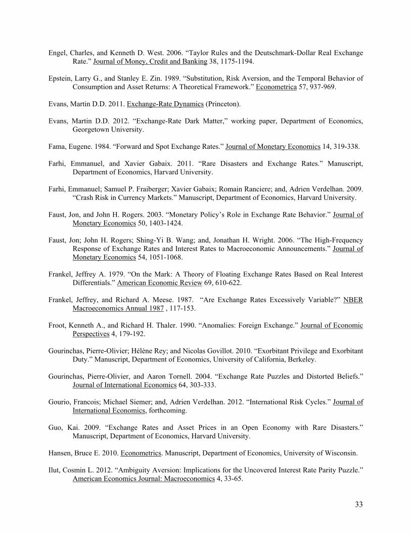
33

Engel, Charles, and Kenneth D. West. 2006. “Taylor Rules and the Deutschmark-Dollar Real Exchange Rate.” Journal of Money, Credit and Banking 38, 1175-1194.

Epstein, Larry G., and Stanley E. Zin. 1989. “Substitution, Risk Aversion, and the Temporal Behavior of

Consumption and Asset Returns: A Theoretical Framework.” Econometrica 57, 937-969. Evans, Martin D.D. 2011. Exchange-Rate Dynamics (Princeton). Evans, Martin D.D. 2012. “Exchange-Rate Dark Matter,” working paper, Department of Economics,

Georgetown University. Fama, Eugene. 1984. “Forward and Spot Exchange Rates.” Journal of Monetary Economics 14, 319-338. Farhi, Emmanuel, and Xavier Gabaix. 2011. “Rare Disasters and Exchange Rates.” Manuscript,

Department of Economics, Harvard University. Farhi, Emmanuel; Samuel P. Fraiberger; Xavier Gabaix; Romain Ranciere; and, Adrien Verdelhan. 2009.

“Crash Risk in Currency Markets.” Manuscript, Department of Economics, Harvard University. Faust, Jon, and John H. Rogers. 2003. “Monetary Policy’s Role in Exchange Rate Behavior.” Journal of

Monetary Economics 50, 1403-1424. Faust, Jon; John H. Rogers; Shing-Yi B. Wang; and, Jonathan H. Wright. 2006. “The High-Frequency

Response of Exchange Rates and Interest Rates to Macroeconomic Announcements.” Journal of Monetary Economics 54, 1051-1068.

Frankel, Jeffrey A. 1979. “On the Mark: A Theory of Floating Exchange Rates Based on Real Interest

Differentials.” American Economic Review 69, 610-622. Frankel, Jeffrey, and Richard A. Meese. 1987. “Are Exchange Rates Excessively Variable?” NBER

Macroeconomics Annual 1987 , 117-153. Froot, Kenneth A., and Richard H. Thaler. 1990. “Anomalies: Foreign Exchange.” Journal of Economic

Perspectives 4, 179-192. Gourinchas, Pierre-Olivier; Hélène Rey; and Nicolas Govillot. 2010. “Exorbitant Privilege and Exorbitant

Duty.” Manuscript, Department of Economics, University of California, Berkeley. Gourinchas, Pierre-Olivier, and Aaron Tornell. 2004. “Exchange Rate Puzzles and Distorted Beliefs.”

Journal of International Economics 64, 303-333. Gourio, Francois; Michael Siemer; and, Adrien Verdelhan. 2012. “International Risk Cycles.” Journal of

International Economics, forthcoming. Guo, Kai. 2009. “Exchange Rates and Asset Prices in an Open Economy with Rare Disasters.”

Manuscript, Department of Economics, Harvard University. Hansen, Bruce E. 2010. Econometrics. Manuscript, Department of Economics, University of Wisconsin. Ilut, Cosmin L. 2012. “Ambiguity Aversion: Implications for the Uncovered Interest Rate Parity Puzzle.”

American Economics Journal: Macroeconomics 4, 33-65.

34

Jordà, Òscar, and Alan M. Taylor. 2012. “The Carry Trade and Fundamentals: Nothing to Fear but FEER

Itself.” Journal of Interniational Economics 88, 74-90. Kim, Soyoung, and Nouriel Roubini. 2000. “Exchange Rate Anomalies in the Industrial Countries: A

Solution with a Structural VAR Approach.” Journal of Monetary Economics 45, 561-586. Lustig, Hanno; Nikolai Roussanov; and, Adrien Verdelhan. 2011. “Common Risk Factors in Currency

Markets.” Review of Financial Studies 24, 3731-3777. Lustig, Hanno, and Adrien Verdelhan. 2007. “The Cross Section of Foreign Currency Risk Premia and

Consumption Growth Risk.” American Economic Review 97, 89-117. Mark, Nelson. 2009. “Changing Monetary Policy Rules, Learning, and Real Exchange Rate Dynamics.”

Journal of Money, Credit and Banking 41, 1047-1070. Martin, Ian. 2012a. “Consumption-Based Asset Pricing with Higher Cumulants.” Review of Economic

Studies, forthcoming. Martin, Ian. 2012b. “The Forward Premium Puzzle in a Two-Country World.” National Bureau of

Economic Research, working paper no. 17564. Meese, Richard, and Kenneth Rogoff. 1988. “Was It Real? The Exchange Rate – Interest Differential

Relation over the Modern Floating-Rate Period.” Journal of Finance 43, 933-948. Morley, James C.; Charles R. Nelson; and, Eric Zivot. 2003. “Why Are the Beveridge-Nelson and

Unobserved Components Decompositions of GDP So Different?” Review of Economics and Statistics 85, 235-243.

Moore, Michael J., and Maurice J. Roche. 2010. “Solving Exchange Rate Puzzles with Neither Sticky

Prices Nor Trade Costs.” Journal of International Money and Finance 29, 1151-1170. Rogoff, Kenneth. 1996. “The Purchasing Power Parity Puzzle.” Journal of Economic Literature 34, 647-

668. Scholl, Almuth, and Harald Uhlig. 2008. “New Evidence on the Puzzles: Results from Agnostic

Identification on Monetary Policy and Exchange Rates.” Journal of International Economics 76, 1-13.

Verdelhan, Adrien. 2010. “A Habit-Based Explanation of the Exchange Rate Risk Premium.” Journal of

Finance 65, 123-146.

Table 1

Fama Regressions: * *1 , 1( )t t t t s s t t s ti s s i i i u

1979:6-2009:10

Country ˆs 90% c.i. ( ˆ

s ) ˆs 90% c.i. ( ˆ

s ) Canada -0.045 (-0.250,0.160) 2.271 (1.186,3.355) France -0.028 (-0.346,0.290) 1.216 (-0.171,2.603)

Germany 0.192 (-0.136,0.520) 2.091 (0.599,3.583) Italy 0.032 (-0.325,0.389) 0.339 (-0.680,1.359) Japan 0.924 (0.504,1.343) 3.713 (2.390,5.036)

United Kingdom -0.410 (-0.768,-0.051) 3.198 (1.170,5.225) G6 0.054 (-0.184,0.292) 2.467 (0.769,4.164)

Notes: 90 percent confidence intervals in parentheses.

Table 2 Fama Regression in Real Terms: 1 , 1ˆ ˆd d

t t t q q t q tq q r r u 1979:6-2009:10

Model 1 Model 2

Country ˆq 90% c.i.( ˆ

q ) ˆq 90% c.i.( ˆ

q ) ˆq 90% c.i.( ˆ

q ) ˆq 90% c.i.( ˆ

q )

Canada 0.021 (-0.170,0.212) (-0.159,0.166) (-0.135,0.157)

0.862 (-0.498,2.222) (-0.632,2.908) (-0.676,2.800)

0.022 (-0.170,0.214) (-0.159,0.168) (-0.136,0.165)

0.851 (-0.523,2.225) (-0.683,2.827) (-0.668,2.739)

France -0.080 (-0.399,0.239)

(-0.281,0.052) (-0.294,0.054)

1.576 (-0.117,3.269) (0.281,3.240) (-0.125,3.602)

-0.075 (-0.397,0.247) (-0.286,0.064) (-0.290,0.064)

1.526 (-0.213,3.265) (0.267,2.964) (-0.260,3.485)

Germany -0.042 (-0.341,0.257)

(-0.209,0.082) (-0.207,0.081)

1.837 (-0.015,3.689) (0.687,4.458) (0.589,4.419)

-0.043 (-0.341,0.255) (-0.206,0.086) (-0.205,0.079)

1.912 (0.071,3.753) (0.748,4.622) (0.627,4.531)

Italy 0.075 (-0.234,0.384)

(-0.149,0.274) (-0.124,0.261)

0.360 (-1.336,2.056) (-1.087,2.136) (-1.358,2.328)

0.082 (-0.229,0.393) (-0.141,0.278) (-0.116,0.276)

0.267 (-1.426,1.960) (-1.115,2.038) (-1.465,2.228)

Japan 0.108 (-0.201,0.417)

(0.008,0.336) (0.015,0.326)

2.314 (0.768,3.860) (0.746,4.300) (0.621,4.441)

0.110 (-0.197,0.418) (0.006,0.325) (0.012,0.326)

2.358 (0.815,3.911) (0.889,4.167) (0.737,4.485)

United Kingdom -0.241 (-0.603,0.121)

(-0.574,-0.074) (-0.611,-0.067)

2.448 (0.854,4.042) (0.873,4.614) (1.039,4.846)

-0.228 (-0.588,0.132) (-0.555,-0.073) (-0.588,-0.069)

2.347 (0.789,3.915) (0.998,4.369) (0.973,4.725)

G6 -0.048 (-0.287,0.191)

(-0.210,0.080) (-0.202,0.068)

1.933 (0.318,4.548) (0.510,3.932) (0.473,4.005)

-0.047 (-0.286,0.192) (-0.189,0.082) (-0.181,0.077)

1.914 (0.317,3.511) (0.553,3.909) (0.412,3.861)

Notes: 90 percent confidence interval in parentheses. The first confidence interval is based on Newey-West. The second two are bootstrapped. The first reports a percentile interval bootstrap and the second a percentile-t interval bootstrap. See Appendix for details.

Table 3 Regression of tq on *ˆ ˆt tr r : ,ˆd

t q Q t q tq r u 1979:6-2009:10

Model 1 Model 2

Country ˆQ 90% c.i.( ˆ

Q ) ˆQ 90% c.i.( ˆ

Q )

Canada -48.517 (-62.15,-34.88) (-94.06,-31.41)

(-140.54,-27.34)

-48.962 (-62.73,-35.19) (-92.51,-33.11)

(-139.93,-29.36)

France -20.632 (-32.65,-8.62) (-44.34,-1.27) (-54.26,1.75)

-20.388 (-32.42,-8.35) (-42.53,-3.73) (-52.83,-0.46)

Germany -52.600 (-67.02.-38.18)

(-85.97,-25.35) (-105.29,-19.38)

-52.738 (-67.10,-38.37) (-85.87,-25.88)

(-105.62,-19.06)

Italy -39.101 (-51.92,-26.28) (-67.63,-16.36) (-90.01,-13.70)

-39.550 (-52.46,-26.64) (-67.29,-17.78) (-87.39,-15.45)

Japan -19.708 (-29.69,-9.72)

(-42.01,-1.05) (-46.53,-4.33)

-19.669 (-29.72,-9.61) (-42.79,-0.92) (-46.23,-3.94)

United Kingdom -18.955 (-31.93,-5.98)

(-40.19,-3.08) (-55.94,4.08)

-18.387 (-31.01,-5.76) (-38.63,-3.61) (-52.82,4.95)

G6 -44.204 (-55.60,-32.80)

(-73.17,-23.62) (-82.87,-21.74)

-44.032 (-55.34,-32.72) (-74.89,-22.06) (-82.93,-22.75)

Notes: 90 percent confidence interval in parentheses. The first confidence interval is based on Newey-West. The second two are bootstrapped. The first reports a percentile interval bootstrap and the second a percentile-t interval bootstrap. See Appendix for details.

Table 4

Regression of ˆt on *ˆ ˆt tr r : ˆ ˆd

t t tr u 1979:6-2009:10

Model 1 Model 2

Country ˆ 90% c.i.( ˆ ) ˆ 90% c.i.( ˆ )

Canada 23.610 (15.12,32.10) (12.62,51.96) (11.96,63.71)

24.192 (15.64,32.75) (13.35,53.16) (12.99,71.13)

France 13.387 (1.06,25.72)

(-2.56,36.25) (-6.98,42.40)

14.045 (1.84,26.25) (0.80,35.39) (-3.60,41.27)

Germany 34.722 (19.66,49.78)

(9.34,57.59) (3.68,69.36)

34.816 (19.77,49.87) (10.30,59.11) (5.701,73.54)

Italy 27.528 (17.58,37.48)

(14.98,48.32) (12.51,58.54)

28.400 (18.40,38.40) (16.00,48.83) (13.26,57.41)

Japan 15.210 (4.76,25.66)

(-0.45,37.08) (0.91,38.87)

15.208 (4.71,25.70) (-0.99,37.77) (1.50,38.48)

United Kingdom 14.093 (0.33,27.86)

(0.39,34.46) (-8.70,46.45)

13.575 (0.17,26.98) (-0.11,33.13) (-8.70,44.32)

G6 31.876 (20.62,43.13)

(16.89,54.62) (16.78,60.89)

31.876 (20.78,42.97) (17.39,55.49) (16.33,59.36)

Notes: 90 percent confidence interval in parentheses. The first confidence interval is based on Newey-West. The second two are bootstrapped. The first reports a percentile interval bootstrap and the second a percentile-t interval bootstrap. See Appendix for detail

Figure 1

Canada

1.5

1.0

0.5

0.0

0.5

1.0

1.5

1 4 7 10 13 16 19 22 25 28 31 34Months

brj

bqj

blj

France

2.0

1.5

1.0

0.5

0.0

0.5

1.0

1.5

1 4 7 10 13 16 19 22 25 28 31 34Months

brj

bqj

blj

Germany

2.0

1.5

1.0

0.5

0.0

0.5

1.0

1.5

1 4 7 10 13 16 19 22 25 28 31 34 Months

brj

bqj

blj

Italy

0.8

0.6

0.4

0.2

0.0

0.2

0.4

0.6

0.8

1.0

1.2

1 4 7 10 13 16 19 22 25 28 31 34 Months

brj

bqj

blj

Figure 1

Japan

2.5

2.0

1.5

1.0

0.5

0.0

0.5

1.0

1.5

1 4 7 10 13 16 19 22 25 28 31 34 Months

brj

bqj

blj

U.K.

3.0

2.5

2.0

1.5

1.0

0.5

0.0

0.5

1.0

1.5

1 4 7 10 13 16 19 22 25 28 31 34 Months

brj

bqj

blj

G6

2.5

2.0

1.5

1.0

0.5

0.0

0.5

1.0

1.5

1 4 7 10 13 16 19 22 25 28 31 34 Months

brj

bqj

blj

Figures plot the slope coefficients of these regressions: brj refers to slope in *

1 1 ,ˆ ˆ( ) d j

t t j t j rj rj t r tE r r r u

bqj refers to slope in 1 ,ˆ ˆ( ) d j

t t j t j qj qj t q tE q q r u

blj refers to slope in 1 ,ˆ ( ) ˆd j

jt t j tj tr uE

Figure 2

The line labeled bRj plots estimates of Rj from the regression ,ˆ ˆIP d j

t j Rj Rj t R tq r u

The line labeled bQj plots estimates of Qj from the regression ,ˆd jt j Qj Qj t Q tq r u

The line labeled Model plots the regression coefficient of t jq on dtr implied by a class of models discussed in Section 3

G6 Levels

-60

-50

-40

-30

-20

-10

0

10

20

Months

ModelbQjbRj

Figure 3

1

G6 Levels (Model with 12 lags)

-30.000

-25.000

-20.000

-15.000

-10.000

-5.000

0.000

5.000

1 11 21 31 41 51 61 71 81months

bQj

bRj

G6 Levels (Model with Equity Prices and Government Bond Yields)

-45.000

-40.000

-35.000

-30.000

-25.000

-20.000

-15.000

-10.000

-5.000

0.000

5.000

1 11 21 31 41 51 61 71 81months

bQj

bRj

1

Appendix

Appendix to section 2: Evidence on stationarity of real exchange rates

Table A1 presents standard ADF tests for a unit root. The null is not rejected for any currency except

the U.K. pound at the 10 percent level. The table also includes tests for a unit root based on the GLS test

proposed by Elliott et. al. (1996). These tests show stronger evidence against a unit root – the null is rejected at

the 5% level for three currencies, at the 10% level for two others, and not rejected for the Canadian dollar or

Japanese yen. However, the test statistic is based on the assumption that there may be a trend in the real

exchange rate under the alternative, which is not a realistic assumption for these real exchange rates.

We next follow much of the recent literature on testing for a unit root in real exchange rates by

exploiting the power from panel estimation. The lower panel of Table A1 reports estimates from a panel

model. The null model in this test is:

(43) 1 11

( )ik

it it i i it j it j itj

q q c q q .

Under the null, the change in the real exchange rate for country i follows an autoregressive process of order ik .

Note that the parameters and the lag lengths can be different across the currencies. Under the alternative:

(44) 1 1 11

( )ik

it it i it i it j it j itj

q q q c q q ,

with a common for the currencies.

We estimate for the six currencies from (44).37 We find the lag length for each currency by first

estimating a univariate version of (44), and using the BIC criterion. The estimated value of is reported in

the lower panel of Table 1, in the row labeled “no covariates”.

This table also reports the bootstrapped distribution of . The bootstrap is constructed by estimating

(43), then saving the residuals for the six real exchange rates for each time period. We then construct 5000

artificial time series (each of length 440, corresponding to our sample of 440 months) for the real exchange rate

by resampling the residuals and using the estimates from (43) to parameterize the model.

The lower panel of Table A1, in the row labeled “no covariates” reports certain points of the

distribution of from the bootstrap. We see that we can reject the null of a unit root at the 5 percent level.

We also consider a version of the panel test in which we include covariates. Specifically, we

investigate the possibility that the inflation differential (with the U.S.) helps account for the dynamics of the

real exchange rate. We follow the same procedure as above, but add lagged own relative inflation terms to

equation (44). To generate the distribution of the estimate of , we estimate a VAR in the change in the real

37 We do not include the average G6 real exchange rate as a separate real exchange rate in this test.

2

exchange rate (as in (43)) and the inflation rate. For each country, the real exchange rate and inflation rates

depend only on own-country lags under the null. The bootstrap proceeds as in the model with no covariates.

The bottom panel of Table A1 reports the estimated and its distribution for the model with

covariates in the row labeled “with covariates”. Adding covariates does not alter the conclusion that we can

reject a unit root at the 5 percent level.

Based on these tests, we will proceed to treat the real exchange rate as stationary, though we note that

the evidence favoring stationarity is thin for the Canadian dollar and Japanese yen real exchange rates.

Table A1 Tests for Unit Root in Real Exchange Rates

Univariate Unit Root Tests, 1973:3-2009:10

Country ADF DF-GLS Canada -1.771 -1.077 France -2.033 -2.036*

Germany -2.038 -2.049* Italy -1.888 -1.914† Japan -2.071 -0.710

United Kingdom -2.765† -2.076* G6 -2.052 -1.846†

* significant at 5% level, † significant at 10% level

Panel Unit Root Test, 1973:3-2009:10 Model Estimated Coefficient 1% 5% 10%

No Covariates -0.01705* -0.02199 -0.01697 -0.01485 With Covariates -0.01703* -0.02174 -0.01697 -0.01455

* significant at 5% level

Appendix to section 2.2: Bootstraps

For both bootstraps in the results reported in Tables 2, 3, and 4, we construct pseudo-samples using the

VAR estimates.38 For each pseudo-sample, we estimate the VAR. We estimate all of the regression

coefficients reported in Tables 2, 3 and 4, and calculate the Newey-West standard errors for each of those

regressions. We repeat this exercise 1000 times.

The first confidence interval based on the bootstraps (the second confidence interval reported for each

coefficient estimate) uses the coefficient estimates reported in the tables. Let ˆ refer to any of the coefficient

estimates reported in Tables 2, 3 and 4. From the regressions on the pseudo-samples, we order the coefficient

estimates from these 1000 replications from smallest to largest - 1̂ is the smallest and 1000ˆ be the largest. The

confidence interval reported in the tables is based on ( 950 50ˆ ˆ ˆ ˆ ˆ ˆ[ ( ), ( )] . That is, the reported

38 Initial values are set at the sample means. We generate samples of 865 observations, then use the last 365 observations, corresponding to the length of the time series we use in estimation.

3

confidence interval corrects for the asymmetry in the distribution of ˆi from the regressions on the pseudo-

samples.

Hansen (2010) argues that the first bootstrap method performs poorly when the ˆi do not have a

symmetric distribution. Instead, he recommends the following procedure. As above, let ˆ refer to the

estimated coefficient in the data, and ˆ to be the Newey-West standard error in the data. For each pseudo-

sample i, we will record analogous estimates: ˆi and ˆ i . i is defined by:

ˆ ˆ

ˆi

ii

. We arrange these i

from smallest to largest, so that 1 is the smallest and 1000 is the largest. The third confidence interval

reported for each coefficient estimate is given by 950 50ˆ ˆˆ ˆ[ , ] . It turns out that our two bootstraps

generally produce very similar confidence intervals.