Real exchange rates and real interest differentialspeople.bu.edu/mbaxter/papers/rer.pdf8 M. Baxter,...

Journal of Monetary Economics 33 (1994) 5537. North-Holland

Real exchange rates and real interest differentials

Have we missed the business-cycle relationship?

Marianne Baxter* Unioersity of Virginia, Charlottesville, VA 22901, USA

Received March 1992, final version received December 1993

This paper investigates the link between real exchange rates and real interest differentials over the recent floating-rate period. In contrast to earlier econometric studies, we find evidence of a relationship, with the strongest link at trend and business-cycle frequencies. Because these prior studies focused on high-frequency components of the data, they found no statistical link between real exchange rates and real interest differentials.

Key words: Real exchange rates; Real interest differentials

JEL classification: F30; F41

1. Introduction

This paper investigates the link between real exchange rates and real interest differentials over the recent floating-rate period. On the face of it, there is little reason to expect any relationship between these variables: even the units do not

Correspondence to: Marianne Baxter, Department of Economics, University of Virginia, Charlottes- ville, VA 22901, USA.

*This paper was written for the conference ‘The Transmission of Monetary Policy in Open Economies’ sponsored by the Swiss National Bank, March 19-20, 1992, Gerzensee, Switzerland. This project was begun while the author was a visiting scholar at the Institute for Empirical Macroeconomics; thanks are due to the Institute and the Federal Reserve Bank of Minneapolis for permitting me to use the Board of Governors database. Special thanks go to the Institute’s research assistant, Martyna Werner, who worked overtime assembling the data. Finally, the paper has benefited from the comments of John Campbell, Morris Goldstein, Robert Hodrick, Robert King, Michael Kouparitsas, and Maurice Obstfeld. Any remaining errors are my own.

0304-3932/94/$07.00 0 1994-Elsevier Science B.V. All rights reserved

6 M. Ba.xtrr, Real exchange rates and vecrl interest d@erentiak

- 120

2-

- 100

.-_

2-

I I

'.j

4 I I I I I I I I I I I I I I I1 60 ,974 1976 1978 1980 1982 1984 1986 1988 1490

Fig. I. The dollar and real interest rates.

match. The real exchange rate is the level of the relative price of one country’s goods in terms of another’s; the real interest differential is quoted in percentage points, and is essentially a rate of change. Nevertheless, it is widely believed that such a link does exist. Fig. 1 plots the U.S. trade-weighted real exchange rate uis-a-ois the G-10 countries, together with a measure of the corresponding long-term, ex ante real interest differential.’ The impression from this figure is that the real exchange rate and real interest differential exhibit the same overall shape, although their short-term movements do not appear to be closely related.

Popular theories of exchange-rate determination also predict a link between real exchange rates and real interest differentials. These theories combine the uncovered interest parity relationship with the assumption that the real exchange rate deviates from its long-run level only temporarily. Under these assumptions, shocks to the real exchange rate - which are often viewed as caused by shocks to monetary policy - are expected to reverse themselves over time.’ For example, if the US dollar real exchange rate is above its long-run level

’ This plot is fig. 1 from Edison and Pauls (1993). Nominal interest differentials are converted to ex ante real interest differentials by subtracting a measure of expected inflation, computed via a two- sided, twelve-quarter moving average.

‘One specific example of a theory that predicts such a link is the sticky-price theory of Dornbusch (1976). In this theory the short-run dynamics of the real exchange rate derive from short-term price rigidity. Thus changes in real exchange rates are expected to reverse themselves over time as prices adjust to their new levels.

M. Baxter. Real exchange rates and real interest d@erentials I

vis-a-ois the Deutsche mark, the dollar is expected to depreciate in real terms in the future. To equate ex ante real yields between the U.S. and Germany, the ex ante real yield on U.S. securities must exceed the ex ante real yield on German securities by the expected real devaluation of the dollar over the term of the bonds. Thus there is a predicted link between the level of the real exchange rate and the ex anre real yield differential.

Nevertheless, prior research has failed to uncover a link between real exchange rates and real interest differentials. In particular, Campbell and Clarida (1987) and Meese and Rogoff (1988) use very different econometric methodolo- gies (reviewed in section 4 below), but both reject the hypothesis that there is a statistically significant link between real exchange rates and real interest differentials. Both studies embed the central assumptions of the sticky-price exchange-rate theories; both therefore conclude that these theories are empiri- cally inadequate.

Yet it is hard to look at fig. 1 and not believe that some relationship exists between the real exchange rate and the real interest differential. This paper therefore re-opens investigation of the link between these variables. In contrast to previous studies, our goal is not to test the implications of particular exchange-rate theories, although our results will necessarily have implications for the empirical validity of these theories. Since we are not testing particular theories, we are not bound by the theoretical or statistical restrictions that characterized previous studies. Thus we stand a better chance of uncovering a link between the variables of interest, if one is there to be found.

The paper is structured as follows. Section 2 presents evidence on the link between real exchange rates and real interest differentials, using (i) short-term and long-term interest rates and (ii) both ex ante and ex post measures of the real interest differential, for six country pairs. As noted above, visual inspection of the data suggests that the strongest relationship between real exchange rates and real interest differentials may be in the slow-moving or low-frequency components. This consideration motivated us to filter the variables to isolate low- frequency, medium-frequency, and high-frequency components, and to study the correlations by frequency band. We find that the correlation between real exchange rates and real interest differentials is, in fact, strongest at medium- to-low frequencies. However, there is essentially zero correlation between these variables at high frequencies. This finding explains why previous researchers, who applied a first-difference filter to the data, failed to uncover a significant link between real exchange rates and real interest differentials. The first-difference filter weights the highest frequencies relatively heavily, with little weight on low and medium frequencies (this is discussed more precisely in section 2). By filtering in a way that emphasized the high-frequency movements, these researchers filtered out the components of the data where the link is strongest.

Section 3 briefly reviews the central elements of the sticky-price theories of exchange rates which have the central implication that there exists a strong link

8 M. Baxter, Real exchange rates and real interest d@wntials

between the real exchange rate and the real interest differential. In addition to the assumption that prices adjust slowly to their new equilibrium values in response to shocks, these theories makes several auxiliary assumptions which must hold if there is to be a strong relationship between the real exchange rate and the real interest differential. The most important of these are (i) uncovered interest parity and (ii) ex ante purchasing power parity. In section 4, we first review empirical evidence on each of these ‘building blocks’ of exchange rate theory. Next, we review prior empirical work on the link between real exchange rates and real interest differentials.

Section 5 presents a statistical mode1 of the real exchange rate, in which the real exchange rate is posited to have both permanent and temporary components. We develop a relationship between the real exchange rate and the real interest differential without making the assumptions inherent in the model of section 3; in particular, we allow deviations from uncovered interest parity, and do not impose ex ante purchasing power parity. The statistical mode1 predicts the following. First, the link that should exist in the data is between the temporary component of the real exchange rate and the real interest differential. Second (but related) is the prediction that there should be no cointegrating relationship between real exchange rates and real interest differentials.

Section 6 implements the statistical mode1 of section 5, decomposing the real exchange rate into permanent and temporary components using univariate and multivariate approaches to trend-cycle decomposition, based on prior work by Beveridge and Nelson (198 l), Blanchard and Quah (1989), and King, Plosser, Stock, and Watson (1991). We investigate the hypothesis that the real interest differential is useful in predicting the temporary component of the real exchange rate. We find that, for some country pairs, there is evidence of a significant link between real exchange rates and real interest differentials, and that the link is stronger when the multivariate decomposition is used. Section 7 reviews the main results of the paper and suggests directions for future research.

2. Real exchange rates and real interest differentials: A first look

This section explores the link between real exchange rates and real interest rates over the recent floating-rate period. Using plots of the data and simple summary statistics, we investigate the following three questions. First, is the link between real exchange rates and real interest differentials sensitive to the measurement of real interest rates? Second, is this link equally strong across all (pairs of) countries? Third, at what frequency is this relationship strongest?

2.1. Measuring real interest difJerentia1.s

To investigate the dependence of this link on the term of the interest rate, we examine quarterly data on short-term and long-term government obligations.

M. Baxtrr. Real exchunge rakes and real interest dt$kwztials 9

The short-term interest rates are three-month interest rates for interbank de- posits or, in the case of the U.S., Treasury bills. The long-term interest rates are yields on ten- to fifteen-year government bonds. In the theory sketched in the introduction, the relevant measure of the real return differential is the ex ante

(i.e., expected) real yield differential. Computing a measure of the ex ante real interest differential requires

a measure of expected inflation. There are many ways to proceed in generating a measure of expected inflation: three common approaches are (i) to use survey data on inflationary expectations, (ii) to compute an inflation forecast from a time-series model such as an ARMA model, or (iii) to compute expected inflation by ‘smoothing’ the inflation series using, for example, a long moving average or an exponential smoother (these can be one- or two-sided). In this paper, we compute one-quarter-ahead expected inflation as the forecast from an ARMA (4,l) model of the inflation differential (additive seasonal dummies were used to remove seasonal components from the inflation rates). Ex ante short- term interest differentials are then computed as the nominal interest differential minus this measure of the expected inflation differential.

Ex ante returns on long-term bonds are more problematic to compute, since this requires forecasts of inflation for the term of the bond. While such a forecast can easily be generated from the ARMA model, these models generaliy do not provide good long-term forecasts. One specific worry is that the revisions in the forecasts of long-term inflation which occur between one period and the next may be so large that these dominate movements in the real rates in computation of the ex ante long-term real rates. The two-sided moving average estimate of expected inflation used by Edison and Pauls (1993). as plotted in fig. 1, produces a time series for expected inflation that is very smooth compared with actual inflation, or expected inflation computed from an ARMA model. A drawback of the two-sided moving average method is that it cannot be a rational forecast of inRation differentials since (i) it uses data from time periods in the future and (ii) the forecast errors from such a smooth measure of expected inflation will not be white noise, as is required of rational forecast errors. In this paper, we use the same (one-quarter-ahead) inflation forecast to compute both ex unte short-term differentials and ex ante long-term differentials. While not entirely satisfactory, this approach to measuring ex ante long-term differentials corresponds to the approach (described below) used by Meese and Rogoff (1988) to compute ex post long-term real interest differentials.

As an alternative to computing a measure of ex ante real interest differentials, one can simply use ex post (i.e., realized) real interest differentials. The ex post differential differs from the ex ante differential by the forecast error for the inflation differential. If expectations are rational, the forecast error is a mean- zero, serially uncorrelated random variable. Thus, if there is a relationship between the ex ante real rate differential and real exchange rates, it should be evident using ex post real rates as well, although the ex post differential is more

10 M. Baxter, Real exchange rates and real interest Qjerentials

1.2

1.1

1

0.9

0.6

0.7

0.6

0.5

real exchange rate vs ex ante real interest diierentiil Brwnth interest rates

0.4 72 74 76 76 80 82 64 66 66 SO

date

real exchange rate vs ex ante real interest differential real exchange rate vs ex post real interest dfferantial biwterm interest rates bngterm interest rates

1.2

1.1

1

0.9

0.6

0.7

0.6

0.5

0.4

real exchange rate v-s ax post real iMeres differenti 5mrmth interest rates

72 74 76 76 6062646666 90!

date

8 6

4

2

0

-2

-4

-6

a

-10

-12

-14

1.2 t L ] IO

0.4 E 1 72 74 76 76 80 62 64 66 66 90 92-15

----- real exchange rate: left scale ($/DM) - - - real interest differential: right scale (% per yr)

Fig. 2a. Real exchange rates and real interest differentials: U.S.-Germany.

volatile than the ex ante differential because it contains an additional ortho- gonal random component.

We compute the ex post short-term real interest differential as the three- month nominal yield differential at the end of quarter t minus the inflation differential realized between the end of quarter t and quarter t + 1. We follow Meese and Rogoff (1988) in computing the ex post long-term interest differential by subtracting realized one-quarter interest rates from the long-term interest differential3 Throughout, nominal rates are converted to real rates using the seasonally unadjusted CPI.

3 As noted by Meese and Rogoff, this procedure does not generate true ex post real return differentials, since the inflation rate is not computed over the term of the bond. However, with less than twenty years of data we have only one or two nonoverlapping observations on true ex post, long-term real returns.

M. Baxter, Real exchange rates and real interest differentials 11

real exchange rate vs ex ante real interest diiafantial 3-rnmth intarast rams

5.6 , I 7.5

76 76 60 62 64 66 88 90 92

date

real exchange rate vs ex ante real intarasl diiarantial k3fyt.m i8tarest rates

5.6 , , 7.5

5.5

5.4

5.3

5.2

5.1

5

4.9 76 76 80 62 64 66 66 90 92

real exchange rate vs ax post real intarast di#fmntial 3mmth interest rates

4'g76 76 60 62 64 96 66 90 !

date

32

real exchange rate vs ex pm! real interest differential bnptm interest rates

10

5

0

-5

-10

5.6 ,

10

5

0

-5

-10

-15

4.g[ vv 76 76 60 62 64 66 66 90 92

-15

----- real exchange rate: left scale ($/Yen) - - - real interest differential: right scale (% per yr)

Fig. 2b. Real exchange rates and real interest differentials: U.S.-Japan.

2.2. Plots and summary statistics

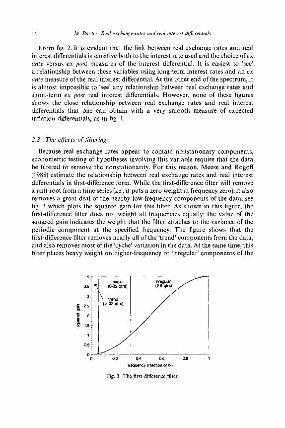
We consider the U.S. vis-a-vis five other countries: France, Germany, Japan, Switzerland, and the U.K., as well as France-Germany. Figs. 2a-2c plot the log of the real exchange rates against the real interest differentials for three country pairs using quarterly data from 1973:l through 1991:2. In each figure (i.e., for each country pair) there are four subpanels, which plot the log of the real exchange rate against four measures of the real interest differential: short- term and long-term, ex ante and ex post.

Figs. 2a and 2b, which plot the real exchange rate of U.S. dollar versus DM and yen, respectively, show the dramatic rise in the value of the dollar from the late 1970s roughly through 1984, followed by its subsequent sharp decline. The subsequent rise and fall of the dollar between approximately 1986 and 1990 was much smaller in magnitude, compared with the earlier period. Fig. 2c illustrates the general decline over time of the French franc in terms of the DM, even

12 M. Baxter, Real exchange rales and real interest djferentials

real exchange rate vs ex ante real interest diierential 5month interest rates

1.4 , , 12

0.9 ’ ’ -9 72 74 76 76 80 82 84 86 86 93 92

dale

real exchange rate vs ex ante real interest ~ffer~~~l long&m bteraat rates

74 76 78 80 62 a4 66 66 90

12

9

6

3

0

-3

-6

-9

date

real exchange rate vs ex post real inter& differential

Smooth interest rates 1.4 I , 12

9 1.3

6

1.2 1 3

1.1 0

-3 1

6

0.9 72

--a 74 76 70 80 82 84 86 88 90 92

1.4

1.3

1.2

1.1

1

real excbartge raters ex post real intwest ~~~1 kli?$wm &teriBt rates

0.9 - 72 74 76 70 80 62 84 96 66 90

date

12

9

6

3

0

3

6

-9

----- real exchange rate: left scale (FF/D~) - - - real interest differ~tial: right scale (% per yr)

Fig. 2~. Real exchange rates and real interest differentials: France-Germany.

though these currencies were tied together via the EMS with occasional align- ments.

Table 1 provides summary statistics on the ex ante and ex post measures of real interest differentials. First, we find that ex ante real interest differentials are about two-thirds as volatile as ex post differentials. Second, ex ante real rate differentials show strong persistence for all country pairs. E‘x post real rate differentials are also positively serially correlated, but in each case the persistence of the ex ante differential is higher than that of the ex post differential. This is what we should expect if individuals form rational expectations of inflation differentials, for under rational expectations the forecast error for the inflation differential should be a white-noise process. Since the ex post differential combines the ex ante differential with the inflation forecast error (i.e., it combines a persistent process with a white noise process), it is expected to exhibit lower persistence than the ex ante differential.

Tab

le

1

Sum

mar

y st

atis

tics

for

real

in

tere

st

diff

eren

tials

. --

-

___-

-

~ -.

___.

- __

____

___

Stan

dard

de

viat

ion

Pers

iste

nce

Cor

rela

tion

- -_

___

Shor

t-te

rm

rate

s L

ong-

term

ra

tes

Shor

t-te

rm

rate

s L

ong-

term

ra

tes

Shor

t-

Lon

g-

--

__.._

_.__

___

term

te

rm

Cou

ntry

pa

ir

Ex

ante

E

x po

st

Ex

ante

E

x po

st

Ex

ante

E

x po

st

Ex

ante

E

x po

st

rate

s ra

tes

-__I

- .~

__

_.-.

__

_ --

.-.

~_

__.

--.

_-

____

-._

____

-.

U.S

.-Fra

nce

2.03

3.

06

1.58

2.

14

0.58

0.

39

0.71

0.

25

0.52

0.

35

U.S

.--G

erm

any

2.46

3.

65

2.78

4.

09

0.67

0.

40

0.90

0.

60

0.66

0.

74

U.S

.-Jap

an

2.08

3.

39

2.24

3.

81

0.52

0.

11

0.84

0.

34

0.55

0.

67

U.S

.--S

witz

erla

nd

2.17

3.

85

2.70

4.

71

0.62

0.

30

0.90

0.

60

0.48

0.

71

U.S

.--U

.K.

3.19

5.

58

2.33

5.

14

0.48

0.

05

0.34

-

0.11

0.

49

0.34

Fr

ance

-Ger

man

y 1.

93

3.72

2.

09

3.66

0.

67

0.39

0.

83

0.46

0.

66

0.63

p 1.

U

nits

ar

e an

nual

ized

pe

rcen

t pe

r qu

arte

r. 2.

Pe

rsis

tenc

e m

easu

re

is t

he

firs

t-or

der

auto

corr

elat

ion

coef

fici

ent.

3.

Cor

rela

tion

is t

he

corr

elat

ion

betw

een

the

ex a

nte

and

ex

post

re

al

inte

rest

di

~ere

ntia

ls.

4.

Sam

ple

peri

ods

are

as

follo

ws.

U

.S.-

Fran

ce:

1973

:4-1

990:

4,

U.S

.-Ger

man

y:

1973

:4-1

991:

1,

U.S

.-Jap

an:

1977

:1-1

991:

1,

U.S

.-Sw

itzer

land

: 19

7.5:

3-19

90:3

, U

.S.-

U.K

.: 19

75:1

--19

91:1

, Fr

ance

-Ger

man

y:

1973

:4-1

990:

4.

w

14 M. Baxter, Real exchange rates and real interesr differentials

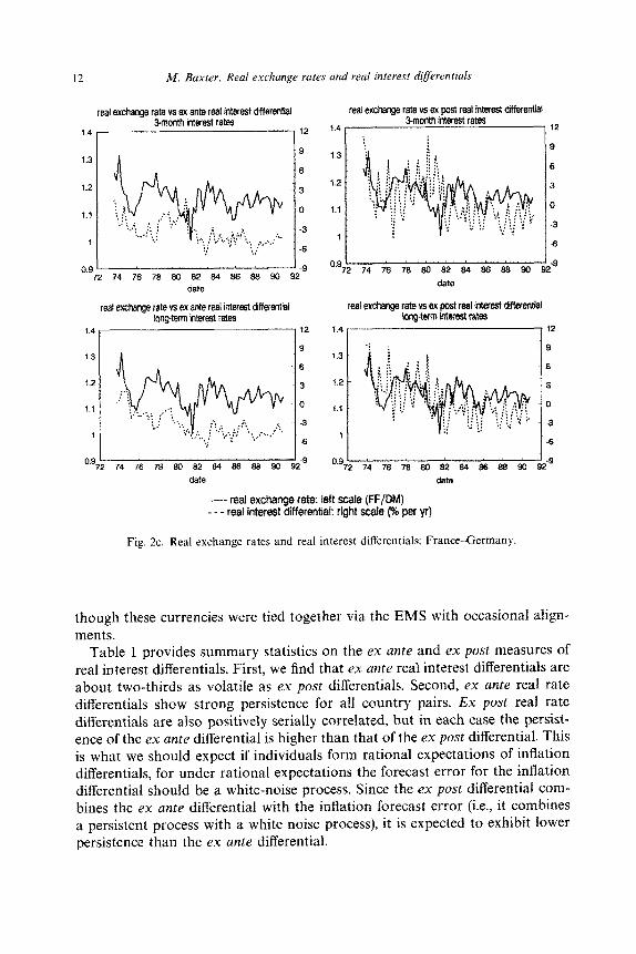
From fig. 2, it is evident that the link between real exchange rates and real interest differentials is sensitive both to the interest rate used and the choice of ex ante versus ex post measures of the interest differential. It is easiest to ‘see’ a relationship between these variables using long-term interest rates and an ex ante measure of the real interest differential. At the other end of the spectrum, it is almost impossible to ‘see’ any relationship between real exchange rates and short-term ex post real interest differentials. However, none of these figures shows the close relationship between real exchange rates and real interest differentials that one can obtain with a very smooth measure of expected inflation differentials, as in fig. 1.

2.3. The clfSects ofjltering

Because real exchange rates appear to contain nonstationary components, econometric testing of hypotheses involving this variable require that the data be filtered to remove the nonstationarity. For this reason, Meese and Rogoff (1988) estimate the relationship between real exchange rates and real interest differentials in first-difference form. While the first-difference filter will remove a unit root from a time series (i.e., it puts a zero weight at frequency zero), it also removes a great deal of the nearby low-frequency components of the data; see fig. 3 which plots the squared gain for this filter. As shown in this figure, the first-difference filter does not weight all frequencies equally: the value of the squared gain indicates the weight that the filter attaches to the variance of the periodic component at the specified frequency. The figure shows that the first-difference filter removes nearly all of the ‘trend’ components from the data, and also removes most of the ‘cyclic’ variation in the data. At the same time, this filter places heavy weight on higher-frequency or ‘irregular’ components of the

frequency (fraction of pi)

Fig. 3. The first-difference filter.

M. Baxter, Real exchange rates and real interest dlrerentials 15

correlation = 0.17 1, ,, ,,1

4

3

2

1

0

-1

-2

-3 76 70 90 92 94 96 99 90 92

-- -- log real exchange rate: left scale ($/DM) - ex post real interest differential: right scale (%)

Fig. 4. Effect of first-difference filter: U.S.-Germany.

data ~ for example, the filter increases by four the variance of cycles in the data which last for two periods (the squared gain is four at frequency n).

To understand how application of this filter alters the data, fig. 4 plots the first-difference of the real exchange rate for the U.S. versus Germany against the first-difference of the ex post long-term real interest differential. There is no evident relationship between the first differences of the real exchange rate and the real interest differential; this impression is confirmed by the low correlation coefficient (0.17). The first-difference filter thus has the unfortunate attribute that it removes a great deal of the low frequencies where, it appears, the link between real exchange rates and real interest differentials may be strongest. Since our goal is to discover whether any link exists between these variables, we do not want to filter our data in a way that biases us against finding this relationship.

Based on these considerations, we chose to proceed by applying approximate band-pass filters to the data on real exchange rates and real interest differentials, and then examining the correlation of these variables by frequency band. In this investigation, we have specified three frequency bands, chosen to correspond to specific definitions of ‘trend’, ‘business-cycle’, and ‘irregular’ movements in the data. Specifically, we define the ‘trend’ component as fluctuations in the data which exceed 32 quarters in length, ‘business-cycle’ fluctuations are cycles of 6-32 quarters in length, and ‘irregular’ fluctuations are those with frequency 2-5 quarters. The approximate band-pass filters used in this analysis are the BP,&, 4) filters described in Baxter and King (1993), where the notation reflects the fact that the filter passes through components of the data with cycles

16 M. Baxter, Real exchange rates and real interest diffrentials

frequency (kaction of pi)

Fig. 5. A business-cycle filter

between p and q periods in length, and the subscript ‘12’ means that 12 leads and lags of the data were used in constructing the filter (i.e., 12 quarterly observations are lost at the beginning and ends of the sample period for the filtered data).4 Fig. 5 plots the squared gain of the business cycle filter [the BP1J6, 32) filter]; this figure shows the way in which the filter approximately isolates those components of the data that lie in this band.

Figs. 6a-6c plot the relationship between the real exchange rate and the long-term ex ante real interest differential, by frequency band, for each country pair. For each country we have plotted the raw data together with the trend, business-cycle, and irregular components. Overall, the trend and business-cycle components of real exchange rates and real interest differentials appear positively correlated, while the irregular components show no consistent pattern.

Table 2 gives the correlations of the filtered components of real exchange rates and real interest differentials for all four measures of the real interest differential. This table confirms the impression from fig. 6: the correlation between real exchange rates and real interest differentials is generally positive at trend and business-cycle frequencies, and is stronger for long-term interest differentials.5 The correlations of the irregular movements (2-5 quarters) are generally close to zero, with many point estimates which are actually negative.

In summary, we have found that a positive relationship exists between real exchange rates and real interest differentials, with the strongest link at trend and business-cycle frequencies. However, there does not appear to be an important

4 For a more detailed discussion of the issues involved in constructing approximate band-pass filters for economic time series, see Baxter and King (1993).

’ The correlations for the trend components may not be meaningful if these are nonstationary. Nevertheless, they may be interpreted as statistics which summarize the within-sample pattern of comovement of the trend components of the time series.

M. Baxter, Real exchange rates and real interest di@rentials 17

raw data “trend” ( > 32 auartersl I 8 , 0.95 5

0.9 .,‘--... 4 0.85 ._

,,’ A_.

0.0 3 .I~.

. 0.75 ,:’ 2 0.7

~

,,,’

.,,’ 1

0.35 ,<I’

.,,’ 0

0.6 _/___..

0.55 -1

t o,576 I

78 00 62 84 a6 af2

date

“cycle” (6-32 quarters) 12.5 008

ml 82 84 86 A-2.5

0.06

0.M

0.02

0

0.02

0.04

0.00

date

“irregular” (2-5 quarters)

----- real exchange rate: lsft scale ($/DM) - - - real interest differential: right scale (% per yr)

Fig. 6a. Components of real exchange rates and real interest differentials: U.S.-Germany.

short-term (high-frequency) link between these variables. This explains why prior research which first-differenced the data failed to find any link - this procedure removed the very components of the data for which the link was strongest.

3. Theory

Popular sticky-price theories of exchange-rate determination predict that, under standard assumptions, there should be a strong statistical relationship between real exchange rates and real interest differentials. This section reviews the central components of these theories, and establishes the notation that will be used in the remainder of the paper.6

In the mid-1970s two competing theories of exchange-rate determination were developed. While both theories stressed monetary disturbances as the central source of short-run fluctuations in exchange rates and interest rates, they

6 This presentation of alternative theories of exchange rate determination owes a great deal to the discussions in section I of Meese and Rogoff (1988) and sections I and II of Frankel (1979).

18 M. Baxter, Real exchange rates and real interest d#erentials

raw data “trend’ ( > 32 quarters) 5.6 6

5.5 .?; ,. ; ; ..: '1 :

5

5.4 ;i ;: r. 4 : .-:

5.3 ‘. ,: : i : : :...i _.' :

; : : :' : 3

; : :..i :.: :; 2

5.2 i:" :*": : : ::

:i 1

5.1 '3 0

: 5 / -1

4.9 b ,’ u -2 5.05 f 80 81 82 33 34 85 36 87 38 80 81 32 33 a4 35 86 37

date date

4

35

3

2.5

2

1.5

1

0.5

0

0.5

“cycle” (632 quarters) “irregular” (2-5 quarters) 0.25 p , IS 005 h ,2

date date

----- real exchange rate: left scale ($/Yen) - - - real interest differential: right scale (% per yr)

Fig. 6b. Components of real exchange rates and real interest differentials: US-Japan.

differed importantly in the channels by which money affected these variables. One theory, developed by Dornbusch and exposited in his (1976) paper, stressed sluggish price adjustment and exchange rate ‘overshooting’. The other theory, developed by Frenkel (1976) and others associated with the University of Chicago, assumed that prices were flexible and stressed the link between expected depreciation of a currency and expected inflation differentials. The two schools of thought nevertheless agreed on two important points: first, that an ‘asset markets’ approach was the correct way to think about exchange-rate determination and, second, that monetary factors were likely the most important determinants of short-run exchange rate movements, while ‘real factors’ became relatively more important later in the adjustment process.

Both theories begin with the assumption that uncovered interest-rate parity holds:’

‘The UIP relationship is more commonly written in the form E,s,+, - s, = brl - &), where s, is the home-country currency per unit foreign currency. In the sticky-price theories of exchange rate determination, this leads to a negatiue relationship between real exchange rates and real interest differentials. 1 have specified the UIP relation in a form that will lead to a positive relationship between these variables, so that it will be easier to see this relationship, if it exists, in the figures presented in the paper.

raw data “trend” ( > 32 quarters) ,O 1.2 ( ,O

;;f L: . 4 .

. . -.. .-.---.- 1.12 .____,,.,....... ._..._

-5

76 82 84 e6 ea “76 L 78 en 02 84 86 as8

data

%ycW (6-32 quarters) ~‘irr~ula~ (2-5 quarters)

date

3

2

1

0

-1

-2

:F

19

-_--- real exchange rate: left scale (FF/DM) - _ - reel interest differential: right scale (% per yr)

Fig. 6c. Components of real exchange rates and real interest differentials: France-Germany.

W,+,c - s,) = - (rR, - km (1)

where kRr and kR: denote the period t nominal yields to maturity on k-period domestic and foreign bonds, respectively, s, denotes the log of the exchange rate, defined as units of foreign currency per unit domestic currency, and E&s,+~ - SJ denotes the expected change in the log exchange rate between periods t and t + k.

The second component common to both theories was the assumption that ex ante purchasing power parity would hold if prices were fully flexible, i.e.,

Eh+k -I- ~t+k - P;F+A = sz + it - PT. (2)

If prices are less than fully flexible, as in the Dornbusch theory, there may be temporary deviations from ex ante purchasing power parity, but this relation is nevertheless assumed to hold in the ‘long run’ when price level adjustments are complete.

The log of the real exchange rate is qt = s, + pt - p,*. Let qt denote the log of the real exchange rate under the assumption that prices are fully flexible; from

20 M. Baxter, Real exchange rates and real interest diffkrentials

Table 2

Frequency-band correlation of real exchange rates and real interest differentials

Country pair Measure of (time period) real interest differential

U.S.-France (1976:4-1987:4)

U.%Germany (1976:4&1988:1)

U.S.-Japan (1980:1-1988:l)

U.S.-Switzerland (1978:3-1987:3)

U.S.-U.K. (1978:lp1988:l)

France-Germany (1976:4-1987:4)

Ex ante: Ex post:

Ex ante: Ex post:

Ex ante: Ex post:

Ex ante: Ex post:

Ex ante: Ex post:

Ex ante: Ex post:

Ex ante: Ex post:

Ex ante: Ex post:

Ex ante: Ex post:

Ex ante: Ex post:

Ex ante: Ex post:

Ex ante: Ex post:

Frequency band (qtrs)

2-5

Short-term Short-term

Long-term Long-term

Short-term Short-term

Long-term Long-term

Short-term 0.16 Short-term 0.11

Long-term Long-term

Short-term 0.17 Short-term 0.22

Long-term Long-term

Short-term -0.14 Short-term 0.25

Long-term Long-term

Short-term - 0.23 Short-term - 0.07

Long-term Long-term

- 0.05 0.10

0.07 0.14

-0.21 0.09

-0.14 0.17

- 0.25 -0.05

0.06 0.18

-0.13 0.26

0.00 0.01

6-32 > 32

0.17 0.08 0.08 -0.09

0.64 0.98 0.45 0.7 1

0.40 0.99 0.51 0.98

0.67 0.98 0.59 0.97

-0.02 0.88 0.26 0.75

0.39 -0.01 0.55 0.08

0.02 0.68 0.18 0.86

0.56 0.96 0.44 0.94

0.12 -0.37 0.16 -0.46

0.18 0.83 0.21 0.80

- 0.40 -0.47

0.22 -0.04

0.57 0.54

0.94 0.83

eq. (2), we have E,qttk = qt. Thus an implication of ex ante purchasing power parity is that St is either constant or a random walk.

In sticky-price theories of exchange-rate determination, the actual value of the real exchange rate, ql, is assumed to follow:’

Et(qt+k - 41 +d = elt - 4th o<e<1.

*In fact, the Dornbusch (1976) and Frankel(l979) expositions of the sticky-price model assumed that expectations of nominal exchange rate changes followed this adaptive process; it is almost the same thing to assume adaptive expectations of real exchange rates, as in Meese and Rogoff (1988). Since this paper is concerned with real exchange rates, we follow Meese and Rogoff.

M. Baxter, Real exchange rates and real interest differentials 21

Combining eqs. (lH3) and defining g, E kRt - (E,P,+~ - pt) as the ex ante real return on domestic bonds (with ,Q-: defined similarly), we have:

4r = 4t + dkr, - kc+?, (4)

where a 3 l/(1 - Ok) > 1. In eq. (4), we have the desired relationship between the real exchange rate and

the real interest differential. Note that this link depends on (i) uncovered interest parity, (ii) ex ante purchasing power parity, and (iii) a specific stochastic process for the real exchange rate, as reflected in eq. (3). In the next section, we review the empirical evidence on each of these ‘building blocks’ which form the foundation for this theory.

4. Prior empirical work

The theories that link the real exchange rate to the real interest differential make three fundamental assumptions: (i) uncovered interest rate parity (UIP), (ii) ex ante purchasing power parity (PPP), and (iii) sticky prices or some other mechanism under which real exchange rates follow eq. (3). This section first reviews empirical evidence on UIP and PPP separately. Second, we review the evidence on ex ante real rate equality which constitutes a test of the joint hypothesis that (i)(ii) hold simultaneously. Finally, we review existing evidence on the statistical properties of real exchange rates and real interest differentials and the linkages between these variables.’

4.1. Uncovered interest parity

Uncovered interest parity states that nominal interest differentials reflect expected movements in exchange rates:

where s, is the log of the spot exchange rate (units of foreign currency per unit domestic currency), kR, is the k-period nominal interest rate in the home country, and kRT is the k-period nominal rate in the foreign country.

Covered interest parity is a no-arbitrage condition under which

(kfl - 4 = - (A - d-V),

9 Cumby and Obstfeld (1984) review the evidence on these ‘building blocks’ of popular exchange rate theories and provide additional empirical evidence. At that time, the evidence was overwhelm- ingly against the hypotheses of uncovered interest parity and ex ante real rate equality. Subsequent empirical studies have not overturned these conclusions.

22 M. Baxter, Real exchange rates and real interest dlflerentials

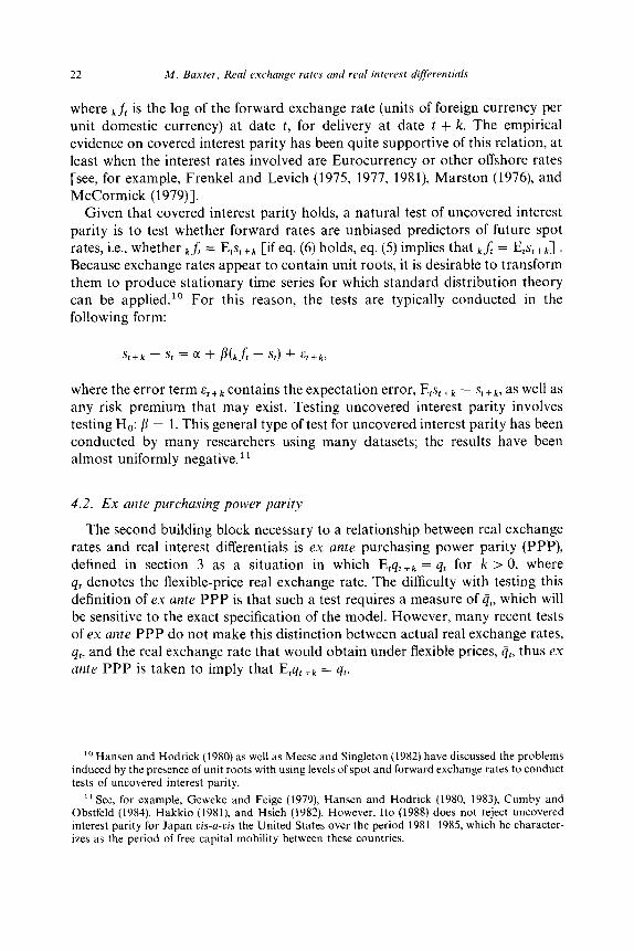
where kff is the log of the forward exchange rate (units of foreign currency per unit domestic currency) at date t, for delivery at date t + k. The empirical evidence on covered interest parity has been quite supportive of this relation, at least when the interest rates involved are Eurocurrency or other offshore rates [see, for example, Frenkel and Levich (1975, 1977, 1981) Marston (1976) and McCormick (1979)].

Given that covered interest parity holds, a natural test of uncovered interest parity is to test whether forward rates are unbiased predictors of future spot rates, i.e., whether kft = E*s,+~ [if eq. (6) holds, eq. (5) implies that kft = E1s,+J Because exchange rates appear to contain unit roots, it is desirable to transform them to produce stationary time series for which standard distribution theory can be applied. lo For this reason, the tests are typically conducted in the following form:

&+k - St = a + b(kft - St) + Et+k>

where the error term E, + k contains the expectation error, E,s, + k - s, + k, as well as any risk premium that may exist. Testing uncovered interest parity involves testing Ho: fi = 1. This general type of test for uncovered interest parity has been conducted by many researchers using many datasets; the results have been almost uniformly negative.”

4.2. Ex ante purchasing power parity

The second building block necessary to a relationship between real exchange rates and real interest differentials is ex ante purchasing power parity (PPP), defined in section 3 as a situation in which E,q,+k = L!$ for k > 0, where qr denotes the flexible-price real exchange rate. The difficulty with testing this definition of ex ante PPP is that such a test requires a measure of &, which will be sensitive to the exact specification of the model. However, many recent tests of ex ante PPP do not make this distinction between actual real exchange rates, qt, and the real exchange rate that would obtain under flexible prices, qr, thus ex ante PPP is taken to imply that E,q,+k = qt.

lo Hansen and Hodrick (1980) as well as Meese and Singleton (1982) have discussed the problems induced by the presence of unit roots with using levels of spot and forward exchange rates to conduct tests of uncovered interest parity.

‘I See, for example, Geweke and Feige (1979) Hansen and Hodrick (1980, 1983) Cumby and Obstfeld (1984) Hakkio (1981) and Hsieh (1982). However, Ito (1988) does not reject uncovered interest parity for Japan vis-a-ok the United States over the period 1981L1985, which he character- izes as the period of free capital mobility between these countries.

M. Baxter, Real exchange rates and real interest diSf&entials 23

4.2.1. Evidence for unit roots

Under the second definition of ex ante PPP (E,q,+k = qJ, ex ante PPP can be tested by testing the null hypothesis that the real exchange rate follows a random walk without drift. The empirical evidence supports the hypothesis that real exchange rates have unit-root components over the post-1973 period. Meese and Rogoff (1988) perform Dickey-Fuller tests on the dollar/mark, dollar/pound, and dollar/yen real exchange rates sampled monthly, and do not reject the null hypothesis of a unit root for any of these exchange rates. In related work, Edison and Pauls (1993) similarly do not reject the hypothesis of unit roots for the above three exchange rates and the U.S. dollar/Canadian dollar rate as well; their analysis used quarterly data.

4.2.2. Evidence for temporary components

However, the existence of permanent components in real exchange rates does not imply that real exchange rates follow a random walk; there may be temporary (mean-reverting) components in the data as well. Tests for the existence of mean reversion in real exchange rates have been carried out by Cumby and Obstfeld (1984), Huizinga (1987) Cumby and Huizinga (1990), and many others.”

Huizinga (1987) used two different approaches to test for mean-reverting components in real exchange rates: (i) the variance-ratio and regression approaches of Cochrane (1988) and Fama and French (1988) and (ii) a univariate Beveridge-Nelson (1981) decomposition of the real exchange rate into permanent and temporary components. Both approaches yielded the same answer: real exchange rates appear to contain both permanent and temporary components. Huizinga also tested for cointegration of real exchange rates with a variety of macroeconomic variables: stock prices, industrial production, real wages, unit labor costs, and productivity. However, he found no support for the hypothesis that real exchange rates are cointegrated with any of these variables.

A novel approach, undertaken by Cumby and Huizinga (1990) was to investigate the hypothesis that the expected change in the real exchange rate over a particular horizon was perfectly correlated with the expected inflation differential over the same horizon, as predicted by ex ante PPP. If changes in real exchange rates were completely unpredictable, the correlation between these two variables should be one. But Cumby and Huizinga find that the estimated correlation is typically small, and is sometimes even negative. Second,

I2 More recently, Mark (1993) has shown that long-horizon changes in nominal exchange rates contain a sizable predictable component - it seems likely that his results would be even stronger for real exchange rates.

24 M. Baxter, Real exchange rates and real interest differentials

Cumby and Huizinga employ a multivariate approach to trend-cycle decomposition. They find that the extracted temporary components to real exchange rates exhibit strong serial correlation, so that real exchange rates lie above or below estimated permanent components for as much as two to three years. Third, Cumby and Huizinga find that as much as 30% of the variance of changes in actual real exchange rates is explained by variance in the temporary components. In summary, recent empirical evidence confirms that real exchange rates contain both permanent and temporary components, leading to a rejection of ex ante purchasing power parity.

4.3. Ex ante real rate equality

Under the combined assumptions that (i) uncovered interest parity holds, (ii) ex ante purchasing power parity holds, and (iii) prices are fully flexible, ex ante real rates should be equalized across countries [set qt = & in eq. (4)]. In the preceding sections we reviewed empirical evidence which casts doubt on each of these assumptions, so it is not surprising that empirical studies of ex ante real rate equality have been almost uniformly negative; see the contributions of Hodrick (1987), Mishkin (1984), and Cumby and Obstfeld (1984).

4.4. Real interest difSerentials and real exchange rates

Empirical work on the link between real exchange rates and real interest differentials has been carried out by a number of authors using a variety of statistical techniques. This section reviews the results of two of the most influential papers, those of Campbell and Clarida (1987) and Meese and Rogoff (1988).13

4.4.1. The Meese and RogofSstudy

Meese and Rogoff (1988) proceed by directly estimating a version of eq. (4). Since real exchange rates appear to be nonstationary, it is undesirable to run this equation in levels. Meese and Rogoff therefore regress the first-difference of the log real exchange rate on seasonal dummies and the ex post long-term real interest differential, using monthly data since 1973, and an instrumental-variables GMM estimator.14 They consider regressions with and without the term &; when included, & is proxied by the cumulated U.S. and foreign trade

I3 In recent work, Clarida and Gali (1993) explore the link between real exchange rates and real interest differentials in a structural-VAR framework.

I4 Meese and Rogoff note (1988, fn. 4, p. 937) that the inflation proxy does not correspond to the term of the long interest rates that they use to construct ex post real rates. Nevertheless, they report that the results are best for the long-term rates.

M. Baxier. Real exchange rates and real interest differentials 25

balances, following the suggestion of Hooper and Morton (1982). The instruments are changes in qrP4 and ( k f 4 - krF_4) for the equations without the trade r balance variables; when these are included, the instrument list includes lagged trade balances as well.

Meese and Rogoff’s main findings are as follows. First, the estimate of c( (the coefficient on the real interest differential) is positive for all three currencies considered: the dollar/mark rate, the dollar/yen rate, and the dollar/pound rate (this is true for equations with and without the trade balance variables). How- ever, none of the estimates of CI is larger than one in absolute value, as predicted by the theory. The standard errors of the estimates are so large, in fact, that conventional tests could not reject in most cases the hypothesis that a = 0. Finally, Meese and Rogoff test for a structural break in the relationship at the Reagan election (November 1980), and strongly reject the null hypothesis of no break. Meese and Rogoff’s own interpretation of these results is as follows:”

‘Our evidence provides no support whatsoever for the view that a model (emphasizing the interaction of sticky prices and monetary disturbances) can explain the major swings in the real exchange rate. The strongest prediction of those models-that real interest differentials will be highly correlated with real exchange rate movements-simply does not appear in the data.’

In the second part of their paper, Meese and Rogoff undertake tests of cointegration of real exchange rates and real long-term interest differentials. They present statistical evidence that real long-term interest differentials are nonstationary, opening up the possibility that these are cointegrated with real exchange rates. l6 However, there is no evidence that real exchange rates are cointegrated with real long-term interest differentials.”

4.4.2. The Campbell-Claridn study

Using a very different econometric methodology, Campbell and Clarida (1987) investigate whether expected real interest differentials can explain a sizable proportion of the variation in real exchange rates, as predicted by sticky- price theories of the exchange rate. Their procedure is to estimate a state-space system in which they impose the following restrictions. First, the long-run real

I5 Meese and Rogoff (1988, para. I, p. 940).

r6As noted by Meese and Rogoff, it is puzzling that real long-term interest-rate differentials should be nonstationary across pairs of countries with highly integrated capital markets. However, a recent study by Cavaglia (1992) finds that real interest differentials are stationary.

I7 Edison and Pauls (1993) use a similar methodology and turn up similar results. Specifically, they fail to find a strong statistical link between real exchange rates and real interest differentials, and they also test and reject cointegration of these variables.

26 M. Baxter, Real exchange rates and real interest dzrerentials

exchange rate is assumed to follow a random walk, with the transitory part of actual real exchange rates identified with ex ante real interest differentials (which are thus assumed to be stationary). Second, uncovered interest parity is assumed to hold exactly; or if it does not, the ‘risk-premium’ term is assumed to be proportional to the ex ante real interest differential. This system contains two unobservable components: expected inflation differentials and the expected long-run real exchange rate. Campbell and Clarida use Kalman filtering techniques to estimate their model under the above assumptions, together with additional identifying assumptions concerning the stochastic process for the unobserved components.

Their findings are as follows. First, the volatility of changes in real exchange rates is about ten times as high as the volatility of real interest differentials. This is not necessarily inconsistent with the theory: the theory predicts that the coefficient c( is greater than one in absolute value, implying that real exchange rates should be more volatile than real interest differentials. Second, they find that most of the movement in real exchange rates is attributable to changes in the permanent component (i.e., the long-run real exchange rate). Third, they find that very little of the movement in real exchange rates is attributable to movement in real interest differentials. As noted by Mishkin (1987), the combi- nation of the Meese-Rogoff results and the Campbell-Clarida study casts serious doubt on the adequacy of the sticky-price theories to explain a link between real exchange rates and real interest differentials. In fact, these authors concluded that there was no statistically significant link between these variables at all. However, their empirical analyses embedded restrictions on the relationship between these variables that are not supported by the data. In the next section, we develop a statistical model of the real exchange rate that relaxes these assumptions, and derives a relationship between the real exchange rate and the real interest differential under these weaker assumptions.

5. A statistical model of the real exchange rate - real interest rate link

This section develops a statistical model of real exchange rates and real interest differentials. Although we shall relax the restrictions imposed by prior theories and empirical work, we maintain a link with the earlier literature by specifying conditions under which our statistical model is identical to models used in prior empirical work.

5.1. Modeling the real exchange rate

Our first point of departure from prior analyses involves permitting deviations from uncovered interest rate parity by including a ‘risk premium’, u,:

Ers,+k - st = - (,A - ,E) + ut.

M. Baxter, Real exchange rates and real interesr d@rentials 27

An expression in the real exchange rate is obtained by adding the term

C(E,p, + k - P,) - (E&+ k - p:)] to both sides of eq. (7):

Note that the ‘error term’ in eq. (8) is identical to the ‘risk premium’ in eq. (7). Next, we specify a statistical model of the real exchange rate. In contrast to

previous studies, we do not require that ex ante purchasing power parity holds. Since Huizinga (1987) and Cumby and Huizinga (1990) found that the real exchange rate has both permanent and temporary components, we specify that

where qf’ is the permanent component of q, and 4: is the temporary component. The permanent component is specified to follow a random walk with drift ,u and with serially-independent innovations $‘:

(10)

An implication of eq. (10) is that predictable changes in real exchange rates are related to predictable movements in the temporary component of real exchange rates:

E&+k - 41 = kp + E,(q,T,k - q,‘,. (11)

Combining eq.(ll) with eq. (8). we find that the predicted link is between real interest differentials and expected changes in the temporary component of real exchange rates. Since variation in temporary components of real exchange rates may be due to a wide range of macroeconomic factors, this analysis suggest the value of a multivariate approach to decomposing the real exchange rate into permanent and temporary components. We follow this approach in section 6.2 below.

5.2. Relationship to sticky-price theories

Before proceeding further, it is useful to ask what restrictions on the stochastic processes for qr and q: lead to the relationship between real exchange rates and real interest rates that was derived from the Dornbusch-Frankel model. The answer is that no further restrictions must be placed on 4:; however, qT must follow an AR(l) process, i.e.,

qT = pq:- 1 + ET. (12)


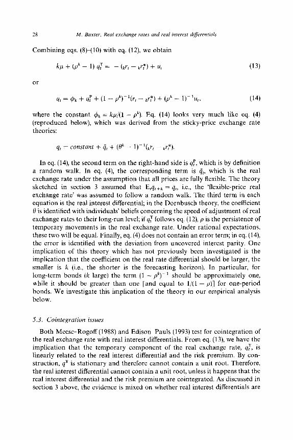
Combining eqs. (SHlO) with eq. (12), we obtain

kp + (p” - 1) q: = - (krf - kr?) + ut (13)

or

qt = $k + 4: + (1 - pk)-l(rt - kr;k) + (p” - l)m’ut, (14)

where the constant @k = kp/(l - pk). Eq. (14) looks very much like eq. (4) (reproduced below), which was derived from the sticky-price exchange rate theories:

qt = constant + cjt + (ok - l)-l(krt - kr:).

In eq. (14), the second term on the right-hand side is qr, which is by definition a random walk. In eq. (4), the corresponding term is &, which is the real exchange rate under the assumption that all prices are fully flexible. The theory sketched in section 3 assumed that E,q,+k = qt, i.e., the ‘flexible-price real exchange rate’ was assumed to follow a random walk. The third term in each equation is the real interest differential; in the Dornbusch theory, the coefficient f3 is identified with individuals’ beliefs concerning the speed of adjustment of real exchange rates to their long-run level; if qf follows eq. (12), p is the persistence of temporary movements in the real exchange rate. Under rational expectations, these two will be equal. Finally, eq. (4) does not contain an error term; in eq. (14), the error is identified with the deviation from uncovered interest parity. One implication of this theory which has not previously been investigated is the implication that the coefficient on the real rate differential should be larger, the smaller is k (i.e., the shorter is the forecasting horizon). In particular, for long-term bonds (k large) the term (1 - pk)-’ should be approximately one, while it should be greater than one [and equal to l/(1 - p)] for one-period bonds. We investigate this implication of the theory in our empirical analysis below.

5.3. Cointegration issues

Both Meese-Rogoff (1988) and Edison-Pauls (1993) test for cointegration of the real exchange rate with real interest differentials. From eq. (13), we have the implication that the temporary component of the real exchange rate, q:, is linearly related to the real interest differential and the risk premium. By con- struction, qT is stationary and therefore cannot contain a unit root. Therefore, the real interest differential cannot contain a unit root, unless it happens that the real interest differential and the risk premium are cointegrated. As discussed in section 3 above, the evidence is mixed on whether real interest differentials are

M. Baxter. Real exchange rates and wal intrrest dtfkwttiais 29

integrated variables; Meese and Rogoff (1988) present evidence that some interest differentials (notably long-term interest differentials) may be nonstationary; both Meese-Rogoff and Cavaglia (1992) find that short-term interest differentials appear stationary. In any case, we see in eq. (14) that the only cointegrating relationship is (trivially) between q1 and 4:. It is worth noting, then, that there is one implication of the sticky-price model that is not rejected by the data: the real exchange rate should not be cointegrated with the real rate diferen- tial!

6. Real exchange rates and real interest differentials once again

The preceding section presented a statistical model of the real exchange rate and derived its implications for the relationship between real exchange rates and real interest differentials. The model predicts that the relationship is between the temporary components of the real exchange rate and the real interest differential. In this section, we use both univariate and multivariate approaches to decomposing the real exchange rate into permanent and temporary components, and then explore whether the hypothesized link exists between temporary components of real exchange rates and real interest differentials.

6.1. Univariate decomposition of’ the real exchange rate

We begin by implementing a univariate decomposition of the real exchange rate into nonstationary (trend) and stationary (cyclic) components, using an approached based on the work of Beveridge and Nelson (1981). Implementing the decomposition requires that we take a stand on the lag length of the autoregressive component of the first difference of the real exchange rate. Two offsetting factors must be considered: (i) arbitrarily truncating the lag length versus (ii) overfitting the data. Huizinga (1987) estimated a univariate Beveridge- Nelson (B-N) decomposition for monthly real exchange rates and used 24 lags. We chose a lag length of 10 quarters for the present study, since the temporary component becomes more important as the lag length is increased, and we wanted to give the data every chance of displaying a link between real exchange rates and real interest differentials.

Table 3a gives the standard deviations of the innovations to the temporary components innovations divided by the standard deviations of the innovations to the permanent components, together with the first four autocorrelations of the temporary components. In each case, the standard deviation of the innovation to the permanent component is larger than the standard deviation of the temporary component. The temporary components are all highly persistent, with first-order autocorrelation coefficients ranging from 0.41 to 0.82.

Table 3b contains information on the cross-country correlations of the innovations to the permanent and temporary components of real exchange

30 M. Baxter, Real exchange rates and real interest d$erentials

Table 3a

Summary statistics: Univariate Beveridge-Nelson decomposition of real exchange ratesa ~~____~

Country pair

Relative volatilityi’ (permanent component vs.

temporary component) PI

Autocorrelations of temporary component

P2 P3 P4

U.S.-France 1.94 0.47 0.27 0.15 - 0.06 US-Germany 1.68 0.78 0.57 0.37 0.10 US-Japan 1.43 0.79 0.63 0.51 0.41 U.S.-Switzerland 1.45 0.82 0.68 0.44 0.24 U.S.-U.K. 2.30 0.41 0.03 0.01 0.11

a Quarterly data, 1976:3-1991:l. b Standard deviation of innovation to permanent component divided by the standard deviation of

the temporary component.

Table 3b

Cross-country correlations of permanent and temporary components of real exchange rates: Univariate Beveridge-Nelson decomposition.

US-France U.S.-Germany U.S.-Japan US-Switzerland U.S.-UK

U.S.-Fra U.S.-Ger U.SJap

(I) Innocations to permanent components

1 .oo 0.55 0.65 1 .oo 0.53

I .oo

(11) Temporary components

US-France U.S.-Germany U.S.-Japan U.S.-Switzerland U.SU.K.

1 .oo 0.63 0.13 1 .oo - 0.31

1 .oo

US-Swi U.SU.K.

0.8 1 0.55 0.65 0.67 0.69 0.56 1 .oo 0.67

1.00

0.39 0.25

0.78 - 0.04 - 0.47 0.44

1.00 - 0.25 1.00

rates. Generally, the cross-country correlation of the innovation to the permanent components is quite high. No clear pattern emerges for the cross-country correlation of the temporary components: a few correlations are strongly positive, while others are approximately zero or even negative.

6.2. Multivariate decompositions

The univariate decompositions computed in section 6.1 above assumed that real exchange rates were a function only of lagged real exchange rates. However,

M. Baxter, Real exchange rates and real interest dlferentials 31

Cumby and Huizinga (1990) tested the hypothesis that nominal exchange rates and the nominal interest differential carried equal and opposite signs in a forecasting equation for the real exchange rates; for most currencies, they marginally reject this hypothesis. They use a bivariate vector autoregression in monthly changes in the real exchange rate and the inflation differential, with twelve lags (and monthly data) to compute a multivariate decomposition. They find, using this technique, that the temporary components of real exchange rates are substantial. We follow Cumby and Huizinga in estimating permanent and temporary components of the real exchange rate from the same bivariate vector

Table 4a

Summary statistics: Multivariate Beveridge-Nelson decomposition of real exchange ratesa

Country pair

Relative volatilityb (permanent component vs.

temporary component) Pl

Autocorrelations of temporary component

PZ P3 P‘S ~~~

U.S.-France 1.72 0.59 0.28 0.20 0.28 U.S.-Germany 0.67 0.92 0.79 0.64 0.50 U.S.-Japan 0.75 0.89 0.80 0.68 0.54 U.S.-Switzerland 0.72 0.91 0.77 0.64 0.55 U.S.-U.K. 2.48 0.46 0.55 0.41 0.27

a Quarterly data, 1976:3-1991:l. b Standard deviation of innovation to permanent component divided by the standard deviation of

the temporary component.

Table 4b

Cross-country correlations of permanent and temporary components of real exchange rates: Multivariate Beveridge-Nelson decomposition.

U.S.-France U.S.-Germany US-Japan U.S.-Switzerland U.S.-U.K.

U.S.-Fra U.S.-Ger U.S.-Jap

(1) Innovations to permanent components

1.00 0.44 0.46 1.00 0.34

1 .oo

(II) Temporary components

U.S.-France U.S.-Germany U.S.-Japan U.S.-Switzerland U.S.-U.K.

1 .oo 0.50 0.33 1.00 0.63

1.00

U.S.-Swi U.S.-U.K.

0.61 0.55 0.65 0.44 0.51 0.40 1.00 0.5 1

1.00

0.28 - 0.01 0.88 - 0.14 0.38 - 0.22 1.00 0.06

1.00

32 hf. Baxter, Real exchange rates and real interest differentials

autoregression, using four lags (and quarterly data). Compared with the univariate decompositions, the temporary component is more important when the multivariate approach is used (except in the U.S.-U.K. case), as shown in table 4a. In fact, with the multivariate decomposition, the volatility of the innovations to the permanent component are now smaller than the volatility of the temporary component for three exchange rates (table 4a). The temporary components exhibit increased persistence with the multivariate decomposition. Table 4b shows that the cross-country correlations of the permanent components are somewhat smaller under the multivariate decomposition but nevertheless continue to be substantial; while the cross-country correlations of the temporary components are generally higher under the multivariate decomposition.

6.3. Interest d@erentials and temporary components of real exchange rates

Having reviewed the statistical properties of the permanent and temporary components of real exchange rates, we turn next to investigating whether the temporary component of real exchange rates is predictable using real interest differentials, as suggested by the theories of sections 3 and 5. We estimate an equation of the form:

qT = constant + c&r, - krt*) + ukt.

We estimate this equation using ex ante and ex post interest rates on both short-term and long-term bonds. For the ex post regressions, we continue in the spirit of Meese and Rogoff, using lagged values of qT and the ex post real return differential as instruments in estimating this equation. The ex ante regressions were estimated using least squares. Standard errors are corrected for possible heteroscedasticity.

The results of this estimation are reported in table 5; panel I reports results for the univariate measure of qT and panel II results for the multivariate measure. Recall that the theory of section 3 predicted that (i) c(~ 2 1 and (ii) elk should be larger the smaller is k; for long-term bonds (k z co), the theory predicts & = 1.

Panel I of table 5 shows that, in most cases, we do not find &+ 2 1. The best results are for the ex post short rates in Germany and Switzerland; these are the only cases in which the point estimate of ak exceeds one. In the German and Swiss cases, the point estimate for the short rate is larger than the point estimate for the long rate, as predicted by the theory. For Japan, we do find that the coefficient estimates for the two long-rate measures are positive, although the short-rate measures yielded negative coefficients. Overall, however, the data show little support for the hypothesis that a strong contemporaneous relationship exists between the temporary component of real exchange rates and alternative measures of the real interest differential.

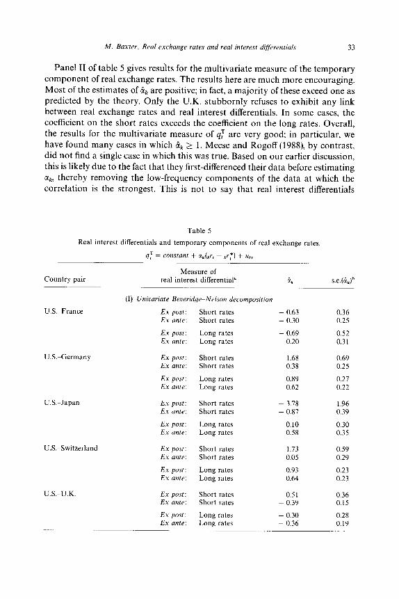
M. Baxter. Real exchange rates and real interest d@wztials 33

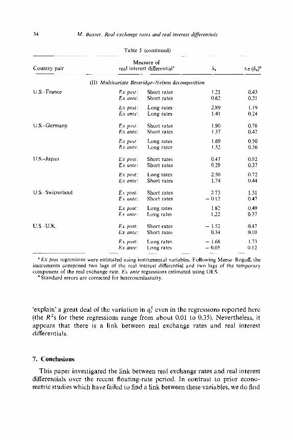
Panel II of table 5 gives results for the multivariate measure of the temporary component of real exchange rates. The results here are much more encouraging. Most of the estimates of kk are positive; in fact, a majority of these exceed one as predicted by the theory. Only the U.K. stubbornly refuses to exhibit any link between real exchange rates and real interest differentials. In some cases, the coefficient on the short rates exceeds the coefficient on the long rates. Overall, the results for the multivariate measure of L$ are very good; in particular, we have found many cases in which Bk 2 1. Meese and Rogoff (1988) by contrast, did not find a single case in which this was true. Based on our earlier discussion, this is likely due to the fact that they first-differenced their data before estimating &, thereby removing the low-frequency components of the data at which the correlation is the strongest. This is not to say that real interest differentials

Table 5

Real interest differentials and temporary components of real exchange rates

qT = constant + cc&r, - ,r:) + ut,

Country pair Measure of

real interest differential” s.e.(&P

U.&France

U.S.PGermany

(1) Univariate BeueridgeeNelson decomposition

Ex post: Short rates - 0.63 0.36 Ex ante: Short rates - 0.30 0.25

Ex post: Long rates - 0.69 0.52 Ex ante: Long rates 0.20 0.31

Ex post: Short rates 1.68 0.69 Ex ante: Short rates 0.38 0.25

Ex post: Long rates 0.89 0.27 Ex ante: Long rates 0.62 0.22

U.S.-Japan

USAwitzerland

Ex post: Short rates - 3.78 1.96 Ex ante: Short rates - 0.87 0.39


Ex post: Short rates 1.73 0.59

Ex ante: Short rates 0.05 0.29


U.S.pU.K. Ex post: Short rates ~ 0.51 0.36 Ex ante: Short rates - 0.39 0.15

Ex post: Long rates - 0.30 0.28 Ex ante: Long rates - 0.36 0.19


Table 5 (continued)

Country pair Measure of

real interest differential” s.e.(d$

U.S.-Japan

US-Switzerland

U.S.-U.K

(II) M&variate Beueridge-Nelson decomposition

U.S.-France Ex post: Ex ante:

Ex post: Ex ante:

Short rates 1.21 0.43 Short rates 0.62 0.21

Long rates 2.89 1.19 Long rates 1.41 0.24

US-Germany Ex post: Ex ante:

Ex post: Ex ante:

Short rates Short rates

Long rates Long rates

Ex post: Short rates Ex ante: Short rates

Ex post: Ex ante:

Long rates Short rates

Ex post: Ex ante:


Ex post: Ex ante:


Ex post: Ex ante:


Ex post: Ex ante:


1.90 0.78 1.37 0.42

1.69 0.50 1.52 0.36

0.47 0.92 0.29 0.37

2.50 0.72 1.74 0.44

2.73 1.31 - 0.12 0.47

1.82 0.49 1.22 0.37

- 1.52 0.47 - 0.34 0.10

- 1.68 1.73 - 0.05 0.12

a Ex post regressions were estimated using instrumental variables. Following MeeseeRogoff, the instruments comprised two lags of the real interest differential and two lags of the temporary component of the real exchange rate. Ex ante regressions estimated using OLS.

b Standard errors are corrected for heteroscedasticity.

‘explain’ a great deal of the variation in qT even in the regressions reported here (the R’s for these regressions range from about 0.01 to 0.35). Nevertheless, it appears that there is a link between real exchange rates and real interest differentials.

7. Conclusions

This paper investigated the link between real exchange rates and real interest differentials over the recent floating-rate period. In contrast to prior econometric studies which have failed to find a link between these variables, we do find

M. Ba.rter. Real exchange rates and real interesf d@erentials 35

evidence of a relationship which can be characterized as follows. First, using band-spectral methods, we found that the strongest correlations between real exchange rates and real interest differentials are found at trend and business cycle-frequencies. There is no relationship between these variables at high frequencies (cycles of 2-5 quarters). This confirms the visual impression obtained from plots of the data: the overall shape of the two time series are similar, but they do not appear highly correlated over short horizons. Our findings explain why prior researchers have had difficulty uncovering a statistical relationship between real exchange rates and real interest differentials: these researchers employed a filter (the first-difference filter) which places most of the weight on the very highest-frequency components of the data.

Next, we reviewed existing theory and the empirical evidence on the ‘building blocks’ of this theory; the maintained hypotheses of uncovered interest parity and ex ante purchasing power parity are found to be poor characterizations of the data. Because of these negative empirical findings, we constructed a statistical model of the link between real exchange rates and real interest differentials which relaxes the counterfactual assumptions of prior theories. This model tells us to look for a link between the temporary component of real exchange rates and the real interest differential. We employed both univariate and multivariate approaches to decomposing time series into permanent and temporary components, and found some evidence that the real interest differential is positively correlated with real exchange rates. This evidence is stronger for the multivariate measure. However, real interest differentials do not explain a great deal of the variance in the temporary components of real exchange rates.

What should we conclude about the link between real exchange rates and real interest differentials? Since real interest differentials are related only to the temporary component of real exchange rates, and since most of the movement in real exchange rates is due to changes in the permanent component, the link between real exchange rates and real interest differentials is necessarily very weak. This may also help explain why prior studies have had so much trouble uncovering a statistically significant relationship. In fact, as summarized above, the link between temporary components of real exchange rates and the real interest differential is itself quite weak. Most of the movement in the temporary component of real exchange rates is attributed, in this study, to the unobserved ‘risk premium’ from the open interest parity relation.

Our findings suggest two fruitful avenues for further research. First, since the data show that the link between real exchange rates and real interest differentials occurs at business-cycle and trend frequency bands, the next step is to construct international macroeconomic models which generate comovement at these frequencies. For example, many of the models discussed in this paper view monetary policy as the driving force behind movements in the real exchange rate and real interest differentials. It remains to be seen whether existing models of this type can produce the observed business-cycle link between these variables.

36 M. Baxter, Real erchangr rates and real intrrest differentials

Second, there is the empirical problem of discovering the underlying causes of movements in real exchange rates and real interest differentials. An early contribution to this literature is Barro (1983); Baxter (1993) also investigated whether an array of policy variables could explain (in a statistical sense) movements in these variables. Both of these studies failed to find policy variables or other macroeconomic variables which could explain movements in real exchange rates or real interest differentials. Thus it remains an open empirical problem to discover the underlying determinants of fluctuations in real exchange rates and real interest differentials.

References

Barro, R.J., 1983, Real determinants of real exchange rates, Manuscript (Department of Economics, University of Chicago, Chicago, IL).

Baxter, M., 1993, Real exchange rates, real interest rates, and government policy: Theory and evidence, Manuscript, Nov. (Department of Economics, University of Virginia, Charlottesville, VA).

Baxter, M. and R.G. King, 1993, Measuring business cycles: Approximate band-pass filters for economic time series, Manuscript, Nov. (Department of Economics, University of Virginia, Charlottesville, VA).

Beveridge, S. and CR. Nelson, 1981, A new approach to the decomposition of economic time series into permanent and transitory components, with particular attention to the measurement of the ‘business cycle’, Journal of Monetary Economics 7, 151-174.

Blanchard, 0. and D. Quah, 1989, The dynamic effects of aggregate supply and demand disturbances, American Economic Review 79, 6555673.

Cavaglia, S., 1992, The persistence of real interest differentials: A Kalman filtering approach, Journal of Monetary Economics 29, 4299444.

Campbell, J.Y. and R.H. Clarida, 1987, The dollar and real interest rates, Carnegie-Rochester Conference Series on Public Policy 27, 103-140.

Clarida, R. and J. Gali, 1993, Sources of real exchange rate fluctuations: How important are nominal shocks?, Manuscript, Oct. (Department of Economics, Columbia University, New York, NY), forthcoming in the Carnegie-Rochester Conference Series on Public Policy.

Cochrane, J., 1988, How big is the unit root component of GNP?, Journal of Political Economy 96, 893-920.

Cumby, R.E. and J. Huizinga, 1990, Investigating the correlation of unobserved expectations: Expected returns in equity and foreign exchange markets and other examples, Manuscript (New York University, New York, NY).

Cumby, R.I. and M. Obstfeld, 1984, International interest rate and price level linkages under flexible exchange rates: A review of recent evidence, in: J. Bilson and R. Marston, eds., Exchange rate theory and practice (University of Chicago Press, Chicago, IL) 121-151.

Dornbusch. R., 1976, Expectations and exchange rate dynamics, Journal of Political Economy 84, 1161~1176.

Edison, J.H. and B.D. Pauls, 1993, A m-assessment of the relationship between real exchange rates and real interest rates: 1974-1990, Journal of Monetary Economics 31, 1499164.

Fama, E. and K. French, 1988, Permanent and temporary components of stock prices, Journal of Political Economy 96, 246-273.

Frankel, J., 1979, On the mark: A theory of floating exchange rates based on real interest differentials, American Economic Review 69, 61@622.

Frenkel, J., 1976, A monetary approach to the exchange rate: Doctrinal aspects and empirical evidence, Scandinavian Journal of Economics 78, 2555276.

Frenkel, J. and R.M. Levich, 1975, Covered interest arbitrage: Unexploited profits?, Journal of Political Economy 83, 325 338.

M. Baxter, Real e.whange rutes and real interest d@rentials 37

Frenkel, J. and R.M. Levich, 1977, Transaction costs and interest arbitrage: Tranquil versus turbulent periods, Journal of Political Economy 85, 120991226.

Frenkel, J. and R.M. Levich, 1981, Covered interest arbitrage in the 1970’s, Economics Letters 8, 2677274.

Geweke, J.F. and E.L. Feige, 1979, Some joint tests of the efficiency of markets for forward foreign exchange, Review of Economics and Statistics 61, 334341.

Hakkio, C.S., 1981, The term structure of the forward premium, Journal of Monetary Economics 8, 41-58.

Hansen, L.P. and R.J. Hodrick, 1980, Forward exchange rates as optima1 predictors of future spot rates: An econometric analysis, Journal of Political Economy 88, 8299853.

Hansen, L.P. and R.J. Hodrick, 1983, Risk averse speculation in the forward foreign exchange market: An econometric analysis of linear models, in: J.A. Frenkel, ed., Exchange rates and international macroeconomics (University of Chicago Press, Chicago, IL).

Hodrick, R.J., 1987, The empirical evidence on the efficiency of forward and futures foreign exchange markets (Harwood, London).

Hooper, P. and J. Morton, 1982, Fluctuations in the dollar: A model of nominal and real exchange rate determination, Journal of International Money and Finance 1, 39-56.

Hsieh, D.A., 1982. Tests of rational expectations and no risk premium in forward exchange markets, National Bureau of Economic Research working paper no. 843.

Huizinga, J., 1987, An empirical investigation of the long-run behavior of real exchange rates, Carnegie-Rochester Conference Series on Public Policy 27, 1499214.

Ito, T., 1988, Use of (time-domain) vector autoregressions to test uncovered interest parity, Review of Economics and Statistics, 2966305.

King, R., C. Plosser, J. Stock, and M. Watson, 1991, Stochastic trends and economic fluctuations, American Economic Review 81, 819-840.

Mark, N., 1993, Exchange rates and fundamentals: Evidence on long-horizon predictability, Manu- script, Aug. (Department of Economics, Ohio State University, Columbus, OH).

Marston, R.C., 1976, Interest arbitrage in the eurocurrency markets, European Economic Review 7, l-13.

McCormick, R., 1979, Covered interest arbitrage: Unexploited profits: A comment, Journal of Political Economy 867, 41 l-417.

Meese, R. and K. Rogoff, 1988, Was it real? The exchange rate-interest rate differential relation over the modern floating-rate period, Journal of Finance 43, 9333948.

Meese, R. and K. Singleton, 1982, On unit roots and the empirical modeling of exchange rates, Journal of Finance 37, 1029-1035.

Mishkin, F.S., 1984, Are real interest rates equal across countries: An empirical investigation of international parity conditions, Journal of Finance 39, 134551358.

Mishkin, F.S., 1987, The dollar and real interest rates: A comment on the Campbell and Clarida paper, CarnegieeRochester Conference Series on Public Policy 27, 141-148.

Obstfeld, M. and K. Rogoff, 1984, Exchange rate dynamics with sluggish prices under alternative price-adjustment rules, International Economic Review 25, 159-174.

Real exchange rates and real interest differentialspeople.bu.edu/mbaxter/papers/rer.pdf8 M. Baxter,...

Documents

Transcript of Real exchange rates and real interest differentialspeople.bu.edu/mbaxter/papers/rer.pdf8 M. Baxter,...