The Method of Steepest Descent - math.uwaterloo.catbury/documents/academic_works/steepe… ·...

AMATH 732 - Asymptotic Analysis and Perturbation Theory

The Method of Steepest Descent

Kamran Akbari, Thomas Bury, Brendon Phillips

November 22, 2015

CONTENTS 1

Contents1 Introduction 2

2 A Review of Asymptotic Methods for Integrals 32.1 Integration of the Taylor Series . . . . . . . . . . . . . . . . . . . . . . . . . . . . . . . . . . . 32.2 What Does Major (Dominant) Contribution Mean? . . . . . . . . . . . . . . . . . . . . . . . . 42.3 Repeated Integration by Parts . . . . . . . . . . . . . . . . . . . . . . . . . . . . . . . . . . . 42.4 Laplace Type integrals . . . . . . . . . . . . . . . . . . . . . . . . . . . . . . . . . . . . . . . . 4

3 The Method of Steepest Descent 63.1 Steepest Path . . . . . . . . . . . . . . . . . . . . . . . . . . . . . . . . . . . . . . . . . . . . . 63.2 The Saddle point . . . . . . . . . . . . . . . . . . . . . . . . . . . . . . . . . . . . . . . . . . . 73.3 How to Find Steepest Paths . . . . . . . . . . . . . . . . . . . . . . . . . . . . . . . . . . . . . 73.4 Laplace Method for Complex Contours . . . . . . . . . . . . . . . . . . . . . . . . . . . . . . . 7

4 Small-amplitude limit of the Korteweg-deVries equation 104.1 Fourier Transform solution . . . . . . . . . . . . . . . . . . . . . . . . . . . . . . . . . . . . . 104.2 Solution curves for various initial conditions . . . . . . . . . . . . . . . . . . . . . . . . . . . . 114.3 Applying the Method of Steepest Descent . . . . . . . . . . . . . . . . . . . . . . . . . . . . . 11

5 Non-linear Steepest Descent and the KdV equation 175.1 Background . . . . . . . . . . . . . . . . . . . . . . . . . . . . . . . . . . . . . . . . . . . . . . 175.2 Posing the Riemann-Hilbert Problem . . . . . . . . . . . . . . . . . . . . . . . . . . . . . . . . 185.3 Deforming Our Riemann-Hilbert Problem . . . . . . . . . . . . . . . . . . . . . . . . . . . . . 20

1 INTRODUCTION 2

1 Introduction

Towards the end of the 19th Century, the Dutch mathematician Gustav de Vries and his supervisor DiederikKorteweg formulated an equation that was to become one of the most famous equations in non-linear wavedynamics. Despite this breakthrough, it was not until the mid 20th Century that further progress was madeon the so-called Korteweg-de Vries (KdV) equation. Many beautiful properties were then discovered, suchas the large time decomposition of the solutions into solitons and in 1967 an analytic solution was foundusing inverse scattering theory.

This project focuses on the method of steepest descent and its application to the long-time asymptoticsof the Korteweg-de Vries equation. We begin by briefly reviewing some of the fundamental ideas and meth-ods for the asymptotic behaviour of integrals. Once the foundation is laid we move onto the theory behindthe method of steepest descent and how it may be applied. Chapter 4 then uses direct application of thismethod on the linearised KdV equation to work out the long-time asymptotic behaviour of the solutions.Chapter 5 approaches the more involved problem of finding the asymptotics for the non-linear KdV equationusing the non-linear variant of the method of steepest descent.

2 A REVIEW OF ASYMPTOTIC METHODS FOR INTEGRALS 3

2 A Review of Asymptotic Methods for IntegralsWe begin with a quick review of the methods of asymptotic evaluation of integrals. The weaknesses andapplicability of each method are analysed. This leads on nicely to the method of steepest descent whichexhibits powerful properties and can be applied to a more diverse range of problems.

2.1 Integration of the Taylor SeriesThe easiest way to form an asymptotic series of an integral is to first expand the integrand into an asymptoticseries, and then integrate term by term. Consider the function f(x) and its Taylor series:

f(x) =

∞∑n=1

un(x).

If un(x) is integrable on interval [a, b], and∞∑n=1

un(x) converges uniformly to f(x), then we can integrate the

Taylor series term by term to obtain the asymptotic behaiviour of the following integral:∫ b

a

f(x)dx =

∞∑n=1

(∫ b

a

un(x)dx

)

There is in fact a weaker condition sufficient for our needs, called Lebesque’s dominated convergence theorem.It says that the partial sums should be bounded, i.e∣∣∣∣ M∑

n=1

un(x)

∣∣∣∣ ≤ Kfor all M and for all a ≤ x ≤ b.

Example:

f(x) =

∫ 1

x

cos t

tdt

cos t

t∼ 1

t− t

2+t3

24−+ . . . →

∫cos t

tdt ∼ ln(t)− t2

2.2!+

t4

4.4!− t6

6.6!+− . . .

For the endpoint t = 1 we have:

−1

4+

1

4.4!+

1

6.6!−+ . . . = C ≈ −0.23981.

Thus, we will have:

→∫ 1

x

cos t

tdt ∼ − ln(x)− C +

x2

2.2!− x4

4.4!+

x6

6.6!−+ . . .

Note that, integrating an asymptotic series term by term gives an asymptotic series, but, this does notalways work for differentiation.


2.2 What Does Major (Dominant) Contribution Mean?To obtain the asymptotic behaviour of integrals, we are concerned with the terms in the integrand that givethe major contribution to the value of the integral. To clarify further, consider the following integral:

I(x) =

∫ x

1

et

tdt

Here, the integral is dominated by ex, that is, in the integrand the term et is dominant to other terms. Infact, it is the exponential function that grows most rapidly in general. In cases where we have terms likeau(t)et as the integrand (so that au(x) grows more rapidly), the ex term is no longer dominant. However, wemay write au(t) as eln au(t) , so, the integrand would be et+ln au(t) . Hence, for integrals involving an exponentialfunction, the only significant part of the integral is the neighbourhood where the exponent is at its maximum.

For our example, the exponential term reaches its maximum when t = x. The lower bound at t = 1 isirrelevant, since the constants are subdominant to the series. Hence, we can write:

I(x) =

∫ x

1

et

tdt =

∫ x−ε

1

et

tdt+

∫ x

x−ε

et

tdt→

∫ x

1

et

tdt ∼

∫ x

x−ε

et

tdt

With the linear transformation: t = x− s, we will have:

→∫ ε

0

ex−s

x− sds = ex

∫ ε

0

e−s

x− sds

Now, by using the Maclaurin series of the term 1x−s ,

1

x− s=

1

x+

s

x2+s2

x3+ . . . ,

and knowing that∫∞

0sne−sds = n!, we will have:

I(x) =

∫ x

1

et

tdt ∼ ex

(1

x+

1

x2+ . . .

)This is a rigorous method of finding the asymptotic behaviour of an integral. It is actually fundamental tothe Laplace method, which we shall talk about in detail later.

2.3 Repeated Integration by Parts

I(x) =

∫ b

a

udv = uv|ba −∫ b

a

vdu

Integration by parts is one of the methods used for asymptotic analysis of integrals. It analyses the integrandnear the boundaries, so this method is useful for asymptotic analysis when the major contribution is nearthe boundaries of [a, b].

2.4 Laplace Type integralsIntegrals of the form

I(k) =

∫ b

a

f(t)e−kφ(t)dt


are said to be in the general form of Laplace integrals. When φ(t) = t, the integral is simply the ordinarytype of Laplace integral (i.e. Laplace transform).

There are three different ways to asymptotically analyse this type of integral.

1. Integration by parts:

As we have seen before, integration by parts is a useful method when the major contributions arenear the boundaries. Here, the exponential function is dominant. So, the major contribution to thisintegral is near the maximum of the exponent, as k → ∞. Because of the minus sign in the expo-nent, we have to find the asymptotic behavior of the integral near the minimum of φ(t). If φ(t) is amonotonic function, the minimum occurs at one of the boundaries. Another point that we should payattention to is that the function f(t) should be sufficiently smooth at the boundary that minimisesφ(t), because we need the value of this function and some of its derivatives at this boundary point.Hence, the integration by parts works in this case. The truncated integration by parts yields

I(k) ∼N∑n=0

(−1)n

(ik)n+1

[f (n)(b)eikb − f (n)(a)eika

], k →∞

In the above formula, the major contribution happens at either a or b, hence we only need include oneof these terms.

2. Watson’s Lemma:

If f(t) is not sufficiently smooth at the boundary of interest, integration by parts no longer works.In this case, Watson suggests that we use the asymptotic power series expansion of f(t). Consider theminimum of φ(t) to be at t = a, and a singularity at this point for f . Thus, the major contributionwould be:

I(k) =

∫ a+ε

a

f(t)e−kφ(t)dt

Now, we expand f(t) near a:

f(t) ∼∞∑n=0

antα+βn, t→ a

Where, α > −1, β > 0, and ε is the radius of validity of the series for f(t). If the end point b is finite,then we should have |f(t)| ≤ A, where A is a constant, for t > 0. When b is infinite, |f(t)| ≤MeCt fort > 0, M constant.

3. Laplace Method:

If φ(t) is not monotonic, the major contribution no longer happens at the boundaries. Thus, wehave to find the asymptotic behaviour of the integral near the minimum of φ, which is in the interiorof the interval. Let c ∈ (a, b) be the value that minimises φ, so φ′(c) = 0 and φ′′(c) > 0. The integralbecomes ∫ c+ε

c−εf(c) exp

{k

(φ(c) +

(t− c)2

2φ′′(c)

)}dt.

3 THE METHOD OF STEEPEST DESCENT 6

Here, we used the Taylor expansion for φ near c. Using the change of variable, τ =√

kφ′′

2 (t − c), wehave

I(k) ∼ e−kφ(c)f(c)

∫ c+ε

c−εexp

{−k (t− c)2

2φ′′(c)

}dt =

e−kφ(c)f(c)√kφ′′/2

∫ −ε√ kφ′′2

+ε

√kφ′′2

e−τ2

dτ

Now, this integral is familiar; as k →∞ the integral is√π. So,

I(k) =

∫ a+ε

a

f(t)e−kφ(t)dt ∼ e−kφ(c)f(c)

√2π

kφ′′(c)

3 The Method of Steepest DescentNow, the goal is to find the asymptotic behaviour of the following integral:

I(k) =

∫C

f(z)ekφ(z)dz, k →∞

where, f(z) and φ(z) are complex analytic functions. The general idea is, by using the analytic characterof the functions, to reform the contour C to another contour C ′ (Cauchy theorem) in which the imaginarypart of the exponent is constant. Hence, the integral would have the form of a Laplace integral, then we usethe rigorous Laplace method. Write

φ(z) = u(x, y) + iv(x, y), z = x+ iy

Supposing, Im{φ} = v is constant in contour C ′, then,

I(k) =

∫C

f(z)ekφ(z)dz = eikv∫C′f(z)ekudz

In order to choose the contour C ′, we usually choose the path of steepest descent passing through z0 inwhich φ′(z0) = 0 (saddle point). We later will show how to find this path. After choosing the path, we haveto find where the major contributions come from. The dominant contributions will happen at critical pointsi.e. where φ′(z) = 0, singular points, and end points. Hence, we have to analyse the integral of the Laplaceform at these points.

3.1 Steepest PathLet φ(z) = u(x, y) + iv(x, y), with z = x + iy; then the paths passing through the point z = z0 (wherev(x, y) = v(x0, y0)) are the paths where the imaginary part of φ is constant. The direction of descent is adirection away from z0 in which u is decreasing; when this decrease is maximal, the path is called the pathof steepest descent. Similarly, the direction of ascent is a direction away from z0 in which u is increasing;when this increase is maximal, the path is called the path of steepest ascent. From calculus we know thatif u(z0) and ∇u 6= 0, then −∇u is the steepest ath decreasing away from u(z0). It is easily shown that thecurves defined by v(x, y) = v(x0, y0) are curves of steepest descent or ascent. If we consider δφ as the changeof the function φ from the point z0, then

δφ = φ(z)− φ(z0) = δu+ iδv → |δu| ≤ |δφ|.

Equality occurs when δu is maximal, so, δv = 0→ v(x, y) = v(x0, y0). This, in fact, shows why we need thesteepest path.


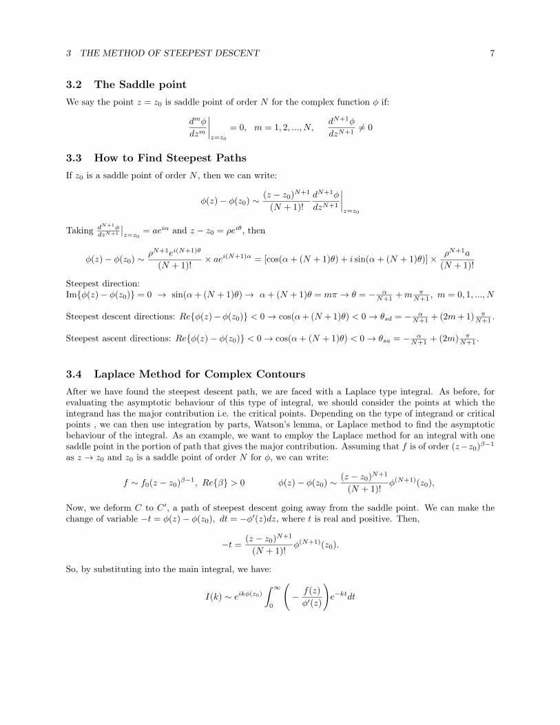
3.2 The Saddle pointWe say the point z = z0 is saddle point of order N for the complex function φ if:

dmφ

dzm

∣∣∣∣z=z0

= 0, m = 1, 2, ..., N,dN+1φ

dzN+16= 0

3.3 How to Find Steepest PathsIf z0 is a saddle point of order N , then we can write:

φ(z)− φ(z0) ∼ (z − z0)N+1

(N + 1)!

dN+1φ

dzN+1

∣∣∣∣z=z0

Taking dN+1φdzN+1

∣∣z=z0

= aeiα and z − z0 = ρeiθ, then

φ(z)− φ(z0) ∼ ρN+1ei(N+1)θ

(N + 1)!× aei(N+1)α = [cos(α+ (N + 1)θ) + i sin(α+ (N + 1)θ)]× ρN+1a

(N + 1)!

Steepest direction:Im{φ(z)− φ(z0)} = 0 → sin(α+ (N + 1)θ)→ α+ (N + 1)θ = mπ → θ = − α

N+1 +m πN+1 , m = 0, 1, ..., N

Steepest descent directions: Re{φ(z)−φ(z0)} < 0→ cos(α+ (N + 1)θ) < 0→ θsd = − αN+1 + (2m+ 1) π

N+1 .

Steepest ascent directions: Re{φ(z)− φ(z0)} < 0→ cos(α+ (N + 1)θ) < 0→ θsa = − αN+1 + (2m) π

N+1 .

3.4 Laplace Method for Complex ContoursAfter we have found the steepest descent path, we are faced with a Laplace type integral. As before, forevaluating the asymptotic behaviour of this type of integral, we should consider the points at which theintegrand has the major contribution i.e. the critical points. Depending on the type of integrand or criticalpoints , we can then use integration by parts, Watson’s lemma, or Laplace method to find the asymptoticbehaviour of the integral. As an example, we want to employ the Laplace method for an integral with onesaddle point in the portion of path that gives the major contribution. Assuming that f is of order (z−z0)β−1

as z → z0 and z0 is a saddle point of order N for φ, we can write:

f ∼ f0(z − z0)β−1, Re{β} > 0 φ(z)− φ(z0) ∼ (z − z0)N+1

(N + 1)!φ(N+1)(z0),

Now, we deform C to C ′, a path of steepest descent going away from the saddle point. We can make thechange of variable −t = φ(z)− φ(z0), dt = −φ′(z)dz, where t is real and positive. Then,

−t =(z − z0)N+1

(N + 1)!φ(N+1)(z0).

So, by substituting into the main integral, we have:

I(k) ∼ eikφ(z0)

∫ ∞0

(− f(z)

φ′(z)

)e−ktdt


Here, we just consider one portion of the path C ′ that gives the major contribution, and we change the upperlimit of integration to ∞ because the major contribution happens near the origin, according to Watson’slemma.

Now, we find the leading behaviour of the term − f(z)φ′(z) :

f(z)

φ′(z)∼ f0(z − z0)β−1

(z − z0)NφN+1(z0)/N != N !

f0(z − z0)β−N−1

φN+1(z0)= N !

f0(ρeiθ)β−N−1

(aeiα)N+1

Plugging this term into the above integral (along with some algebra) gives us:

I(k) ∼ f0[(N + 1)!]β/(N+1)eiβθ

N + 1

ekφ(z0)Γ( βN+1 )

[ka]β/(N+1)

Example: Find the asymptotic evaluation of the integral∫ 1

0log(t)eiktdt as k →∞.

Here we have: φ(z) = iz = i(x + iy) = −y + ix. So, φ′(z) = i, and we have no saddle point. Actu-ally the dominant contribution is the endpoint, and the steepest paths (i.e. Im{φ} = const) are given byx = const. Thus, if y > 0 or y < 0, we are on steepest descent or steepest ascent path, respectively. We haveto choose the path of steepest descent so that it passes through end points. Therefore x = 0, y > 0 and x = 1,y > 0 are the paths of steepest descent going through the endpoints. Notice that Im{φ(0)} = Im{φ(1)};so there is no continuous contour joining t = 0 and t = 1 on which Im{φ} is constant. Hence, we have toconnect these two portions of the steepest descent path. We connect these two contours by another contourat infinity which, by Jordan’s Lemma, will not give any major contribution (the integral over this contour∼ 0). Then, using Cauchy’s theorem, we deform the contour in [0, 1]. Note that, since t = 0 is an integrablesingularity, we shall allow the contour to pass through the origin. Thus, we can write:

I(k) =

∫C1∪C2∪C3

log zeikzdz = i

∫ R

0

log(ir)e−krdr +

∫ 1

0

log(x+ iR)eikx−kRdx− ieik∫ R

0

log(1 + ir)e−krdr

where, according to Figure 1, R→∞. Hence the second integral vanishes and we get

I(k) = i

∫ ∞0

log(ir)e−krdr − ieik∫ ∞

0

log(1 + ir)e−krdr

Figure 1: Contour of integration


Letting s = kr, we get

I1(k) =i

k

∫ ∞0

(log

(i

k

)+ log(s)

)e−sds

Using the results from the familiar integral∫∞

0log(s)e−sds,

I1(k) = − i log k

k−

(iγ + π2 )

k

where, γ = 0.577216... is the Euler constant. For the second integral, we use Watson’s lemma. We knowthat

log(1 + ir) = −∞∑n=1

(−ir)n

n.

So, as k →∞, the complete expansion for the second integral is ieik∞∑n=1

(−i)n(n−1)!kn+1 . Finally, we have

I(k) ∼ − i log k

k− (iγ + π/2)

k+ ieik

∞∑n=1

(−i)n(n− 1)!

kn+1, k →∞

4 SMALL-AMPLITUDE LIMIT OF THE KORTEWEG-DEVRIES EQUATION 10

4 Small-amplitude limit of the Korteweg-deVries equationThe Korteweg-deVries (KdV) equation is a model for waves on shallow water surfaces. Its non-dimensionalform is given by

Vt + 6V Vx + Vxxx = 0 (4.1)

Here we will be investigating the small-amplitude limit of this equation. This can be obtained by settingV = εu in the above equation and taking the limit as ε→ 0. We will thus be working with the equation

ut + uxxx = 0, −∞ < x <∞, t > 0. (4.2)

with initial valuesu(x, 0) = u0(x). (4.3)

Since there are no external energy sources we may assume that u→ 0 sufficiently rapidly as |x| → ∞.

4.1 Fourier Transform solutionEquation (4.2) can be solved using Fourier transforms. Taking u(k, t) to be the Fourier Transform of u in x,we have

u(x, t) =1

2π

∫ ∞−∞

u(k, t)eikxdk. (4.4)

Upon substitution of this form of u into the PDE (4.2) we obtain

∂

∂tu(k, t) + (ik)3u(k, t) = 0 (4.5)

which can be readily solved to giveu(k, t) = u(k, 0)eik

3t. (4.6)

Using the initial condition we have

u0(x) = u(x, 0) =1

2π

∫ ∞−∞

u(k, 0)eikxdk (4.7)

and so we seeu(k, 0) = u0(k)

where u0(k) is the Fourier transform of u0(x) in x. Thus our solution to (4.2) in integral form is given by

u(x, t) =1

2π

∫ ∞−∞

u0(k)eikx+ik3tdk

=1

2π

∫ ∞−∞

u0(k)etφ(k)dk, φ(k) = i

(k3 +

kx

t

)(4.8)

This now has the required form for use of the method of steepest descent, assuming that u0(k) can becontinued analytically off the real k axis.


4.2 Solution curves for various initial conditionsBefore we embark on the method of steepest descents to find the asymptotic behaviour as t → ∞, let usobserve some solution curves for different initial conditions. It is interesting to see the way in which theenergy dissipates for various initial waves. These were constructed using Fast Fourier Transform methodson equation (4.8), using the Python programming language.

(a) Initial wave u0(x) = e−x2

(b) Initial wave u0(x) = xe−x2

Figure 2: Solution curves for fixed t.

4.3 Applying the Method of Steepest DescentExtending (4.8) onto the complex plane, we have the integral

I(t) =1

2π

∫ ∞−∞

u0(z)etφ(z)dz (4.9)

whereφ(z) = i

(z3 +

zx

t

)(4.10)

First, we look for the saddle points z0 of φ. These are points that satisfy φ′(z0) = 0. Differentiating, we have

φ′(z) = i(

3z2 +x

t

). (4.11)

The nature of the saddle points will depend upon the sign of x/t, so we will consider the three cases

(a) xt < 0. This gives two real saddle points z± = ±

∣∣ x3t

∣∣1/2.(b) x

t > 0. This gives two pure-imaginary saddle points z± = ±i(x3t

)1/2.(c) x

t → 0. Now we have the single saddle point z = 0 of higher order which requires a different approachas we shall see.


Recall the equation for the direction of steepest descent θ at a saddle point z0 of order n− 1.

θ = −αn

+ (2m+ 1)π

n, m = 0, 1, ..., n− 1 (4.12)

wherednφ

dzn

∣∣∣∣z=z0

= aeiα. (4.13)

4.3.1 Case (a)

To compute the order of the real saddle points we must compute further derivatives of φ. We see that

φ′′(z±) = ±6i∣∣∣ x3t

∣∣∣ 12 = 6∣∣∣ x3t

∣∣∣ 12 e±iπ2 (4.14)

is non-zero and so these are order one saddle points. Thus our equation for the direction of steepest descentis

θ = −α2

+ (2m+ 1)π

2, m = 0, 1 (4.15)

where α is seen to be ±π2 from (4.14).

So at z+ we have steepest descent directions θ = π4 ,

5π4 . At z− we have steepest descent directions θ = 3π

4 ,7π4 .

This is illustrated in Figure 3.

The next stage is to deform the contour (−∞ < z < ∞) onto the steepest descent contour going throughboth of the saddle points. From the earlier theory, we know that the contours of steepest descent are givenby Imφ(z) = const. In our case then, we have

Imφ(z) = Imφ(z±). (4.16)

This gives a hyperbola as the steepest descent contour. Consider z = |z|eiϕ, ϕ = π/4, 3π/4, for large |z|.Then φ(z) will be dominated by the cubic term and we will have

φ(z) ≈ iz3 = i|z|3e3iϕ = i|z|3(±1 + i) = |z|3(−1± i). (4.17)

Then clearly for large |z|, the exponential etφ(z) will decay rapidly. Thus we can deform our original contouronto the steepest descent contour going through both of the saddle points without any problem.

To find the asymptotic behaviour of I(t), it remains to sum up the contributions to the integral from eachsaddle point. The equation for the contributions is outlined in the theory earlier and in this case is given by

Iz0(t) ∼ u0(z0)eiθetφ(z0)Γ( 1

2 )

(t|φ′′(z0)|) 12

(4.18)

Substituting values in, we obtain the two contributions

u0

(∣∣ x3t

∣∣ 12) e−2it| x3t |32 + iπ

4

2√πt∣∣ x

3t

∣∣ 14 andu0

(−∣∣ x

3t

∣∣ 12) e2it| x3t |32− iπ4

2√πt∣∣ x

3t

∣∣ 14 . (4.19)


(a) Steepest descent directions (b) Deformation of the contour

Figure 3: Saddle point illustrations for the case where xt < 0.

These contributions form a conjugate pair. Write

u0

(∣∣∣ x3t

∣∣∣ 12) = ρ(∣∣∣xt

∣∣∣) eiψ( xt ) (4.20)

then adding the contributions gives

u(x, t) ∼ρ(xt

)√πt∣∣ x

3t

∣∣ 14 cos

(2t∣∣∣ x3t

∣∣∣ 32 − π

4− ψ

(xt

))as t→∞, x

t< 0. (4.21)

4.3.2 Case (b)

We now consider the case where xt > 0. This gives two complex roots for φ′(z) = 0 given by

z± = i

√x

3t. (4.22)

We then compute

φ′′(z±) = ∓6

√x

3t(4.23)

which in the form of (4.13) has a = 6√

x3t and α = π, 0. Note also that since φ′′(z±) 6= 0, these saddle points

are of first order. The direction of steepest descent at these saddle points can then be computed using (4.12).For z+ we get θ = 0, π. For z− we get θ = π/2, 3π/2. This is illustrated in Figure 4.

Writing z as z = zR + izI for zR, zI ∈ R, we find that

Imφ(z) = zR

(z2R − 3z2

I +x

t

). (4.24)


(a) Steepest descent directions (b) Deformation of the contour

Figure 4: Saddle point illustrations for the case where xt > 0

One can also calculate

φ(z±) = ∓2( x

3t

) 32

(4.25)

which we see is real. The contours of steepest descent that go through the saddle points z± satify

Imφ(z) = Imφ(z±) (4.26)

⇒ zR

(z2R − 3z2

I +x

t

)= 0. (4.27)

At z+, it is the hyperbola z2R − 3z2

I + x/t = 0 that is consistent with the direction of steepest descent. Wecan deform the original contour onto the upper half plane part of this hyperbola, since the exponential etφdecays exponentially in this region. The exponential grows in the lower half plane, so we cannot use thepath going through z−.Using equation (4.18) to find the contribution of z+ to the integral we get

u(x, t) ∼u0

(i(x3t

) 12

)e−2t( x3t )

32

2√πt(

3xt

) 14

, t→∞, x

t> 0. (4.28)

4.3.3 Case (c)

In the case where xt → 0 our asymptotic expressions for u derived thus far break down due to the occurrence

of xt in the denominator. The way around this is to introduce the similarity variables

ξ = k(3t)12 , η =

x

(3t)12

. (4.29)


The expression for u in (4.8) becomes

u(x, t) =1

2π(3t)13

∫ ∞−∞

u0

(ξ

(3t)13

)eiξη+ iξ3

3 dξ (4.30)

For large t we may Taylor expand u0 near ξ = 0 to give the asymptotic expression

u(x, t) ∼ 1

2π(3t)13

∫ ∞−∞

eiξη+ iξ3

3

(u0(0) +

ξ

(3t)13

u′0(0) + . . .

)dξ as t→∞. (4.31)

Recall the Airy function Ai(η) is the solution to the differential equation

Aηη − ηA = 0 (4.32)

that satisfies A(η)→ 0 as η →∞. One can verify that it can be written in integral form as

Ai(η) =1

2π

∫ ∞−∞

eiξη+ iξ3

3 dξ (4.33)

which is what we observe in (4.31). Note that each derivative of Ai(η) includes an extra factor of iξ, whichaccommodates the higher order terms in (4.31). Thus we can write

u(x, t) ∼ (3t)−13 u0(0)Ai(η)− i(3t)− 2

3 u′0(0)Ai′(η) as t→∞. (4.34)

4.3.4 Asymptotic Matching of solutions

We should check that our asymptotic solution for u in the region where xt → 0 (the inner region) matches

smoothly with the solution in the two outer regions. For this, we will need the asymptotic behaviour of theAiry function, given by

Ai(η) ∼ 1

2√πη

14

e−23η

32 as η →∞ (4.35)

Ai(η) ∼ 1√π|η| 14

cos

(2

3|η| 32 − π

4

)as η → −∞. (4.36)

The leading order solution for u in the inner region is given by

u(x, t) ∼ (3t)−13 u0(0)Ai(η) as t→∞ (4.37)

Taking the limit as η →∞ gives

u(x, t) ∼ (3t)−13 u0(0)

2√πη

14

e−23η

32 as t→∞ (4.38)

=u0(0)

2√πt

(t

3x

) 14

e−2t( x3t )3/2

(4.39)


which is in accordance with the right outer solution (4.28) upon Taylor expanding u0 and keeping the leadingorder term.

Taking the limit as η → −∞ gives

u(x, t) ∼ (3t)−13 u0(0)

√π|η| 14

cos

(2

3|η| 32 − π

4

)as t→∞ (4.40)

=u0(0)√πt∣∣ x

3t

∣∣ 14 cos

(2t∣∣∣ x3t

∣∣∣ 32 − π

4

)(4.41)

which agrees nicely with the leading order solution in the left outer region (4.21).

5 NON-LINEAR STEEPEST DESCENT AND THE KDV EQUATION 17

5 Non-linear Steepest Descent and the KdV equation

AbstractThe method of nonlinear steepest descent was developed and applied to the canonical Korteweg-de

Vries (KdV) and modified KdV (mKdV) equations by Deift and Zhou in [2, 3], and further expounded byKamvassis in [5]. Grunert and Teschl then applied the method to the KdV equation in [4]; in this sectionof the presentation, we will closely follow Grunert’s approach in [4] to find the asymptotic behaviour ofthe solution in the soliton region x > βt for some positive constant β > 0. Since q(−x,−t) is a solutionof the KdV equation if and only if q(x, t) is, we only investigate the behaviour of the solution for largepositive t.

5.1 BackgroundFirst we gather the necessary information from Scattering Theory. As outlined in [4, 6, 11], we start withKdV equation, given as

∂tq − 6q∂xq + ∂3xq = 0

Consider the connection between the KdV equation and the Schrödinger operator H(t) = −∂2x + q defined

on H2 (order-2 Sobolev space), where the potential q = q(x, t) is a solution of the KdV equation. Thecorresponding eigenvalue problem is given by

−∂2Φ

∂x2+ q(x, ∗)Φ = λ2Φ, λ = a+ ib (5.1)

with the assumption that the solution decays quickly (‖(1 + |x|)q(x, ∗)‖L1 <∞). Whenever b > 0, thereexists a unique pair of (eigenvalue-dependent) analytic solutions ψ±(λ, x, ∗) called Jost solutions, implicitlydefined by

ψ±(λ, x, ∗) = e±iλx ± 1

λ

∫ ±∞x

sin(λ(x− y))q(y, t)ψ±(λ, x, ∗) dy

and which behave asymptotically like e±iλx as x→ +∞ [6]. If λ ∈ R, then ψ± is also a pair of solutions of(5.1), and is linearly independent to ψ±, since the Wronskian determinant of the pair (taking functions withcorresponding signs) is 2iRe(λ). We then have the relation

ψ− =1

2iRe(λ)[ψ+, ψ−]︸︷︷︸

f(a)

·ψ+ +1

2iRe(λ)

[ψ−, ψ+

]︸︷︷︸

g(a)

·ψ+

Tanaka [11] interprets f(a) (respectively, g(a)) as the boundary value of the analytic function f(λ) (resp.g(λ)). Also, the roots of f are finite, simple and purely imaginary1 (since ψ±(λ, x, ∗) ∈ L1(R) ∩ L2(R) at

1By the Spectral Theorem for Self-Adjoint Differential Operators, the spectrum of (5.1) splits into a continuous part (λ > 0)and a discrete part (λ < 0). Denote the discrete eigenvalues as iλ1, iλ2, . . . , iλn, and their corresponding bound states ψn(x, t) ∈L2(R). The reflection and transmission coefficients R(λ) and T (λ) are recovered from the continuous spectrum by looking atthe asymptotic behavior of the eigenfunctions:

ψ ∼{T (λ) eiλx x→ +∞R(λ) e−iλx x→ −∞


the roots of f); say that they are {iλj}1≤j≤n.

The reflection coefficient is given by the function R =g

f, and the norming constants are defined as

γj(t) =1

‖ψ+(iλj , ∗, t)‖2=

1∫R |ψ+(iλj , ∗, t, )|2 dx

The scattering data is the set {R(a), λj , γj(∗)}j , with its time evolution given by the relations2

R(k, t) = R(λj)e8ik3t γj(t) = γje

4λ3j t γj = γj(0), R(λj) = R(λj , 0)

We also have the relation

T (k)ψ±(k, x, t) = ψ±(k, x, t) +R±(k, t)ψ±(k, x, t)

where R± denotes the left and right reflection coefficients. The asymptotic behaviour of the Jost solutionswith respect to k is given in [2, 4] as

ψ± ∼(

1 +Q±(x, t)1

2ik+O

(1

k2

))e±ikx as k → +∞, Q± = ∓

∫ ±∞x

q(y, t) dy (5.2)

Lemma 1 (Properties of the Reflection and Transmission Coefficients [4])

1. T (k) ∈ C1(C \ R) is meromorphic on H+ with simple poles {iλj}1≤j≤n

2. Res [T (k), iλj ] =ψ+

ψ−(iλj , x, ∗)γ2

j (∗)

3. T (k)R+(k, t) = −T (k)R−(k, t) and |T (k)|2 + |R±(k, t)|2 = 1

5.2 Posing the Riemann-Hilbert ProblemWe start with the following definitions.

Definition 1 (Sectionally Analytic Function)A sectionally analytic function is a function Φ defined by a Cauchy-type integral

Φ(z) =1

2πi

∮Γ

φ(s)

s− zds

where φ(s) is Hölder continuous on the compact curve Γ. Notice that Φ(z) ∼(

12πi

∮Γφ(s) ds

)1z as |z| → ∞.

�

Definition 2 (Riemann–Hilbert problem [7, 8])Let Γ be an oriented contour (that is, an oriented non-intersecting Hölder-continuous union of smooth curves)Γ ⊂ C, and a smooth jump matrix V : Γ → M2×2(C). The problem is that of finding a matrix-valuedfunction Υ : C \ Γ → M2×2(C) partitioning the plane into the interior and exterior regions D+ and D−respectively. Υ is (sectionally) analytic on C \ Γ = D+ ∪D−, with Υ+(z) = Υ−(z)V (z) for all z ∈ Γ, anduniqueness of solution guaranteed by the normalisation Υ(∞) = I2×2. Here, Υ±(z) denotes lim

z→Γ±Υ(z), and

Υ(∞) = lim|z|→∞

Υ(z), where Υ± must exist and be continuous. �

2Tanaka [11] gives the evolution of the norming constant as γj(x, t) = γje8λ3j t.


In the previous section, we dealt with the linear variant of the method of steepest decent. Here, we moveto the nonlinear variant. The main difference between the methods is that the linear method calls for thedeformation of the contour of integration onto the path of stationary phase, while the nonlinear method callsfor deformation of the Riemann-Hilbert (hereafter written RH) problem (by conjugating the jump matrix)into a form that is exactly soluble [5, 9]3.

Here, we offer the first formulation of our KdV RH problem:

Vector Riemann-Hilbert Problem 1 ([4, 6])Find a Υ(k) = Υ(k, x, t) meromorphic on C \ R with simple poles at ±iλj so that

1. Υ+(k) = Υ−(k)

[1− |R(k)|2 −R(k)e−φ(k,t)

R(λ)eφ(k,t) 1

](jump condition)

2. Res[Υ(k), iλj ] = γ2j eφ(iλj ,t) lim

k→iλjΥ(k)

[0 0i 0

](pole condition)

3. Υ(−k) = Υ(k)

[0 11 0

](symmetry condition)

4. Υ(+i∞) =[1 1

](normalisation)

where the phase of the solution is given by φ(k, t) = 2ikx+ 8ik3t, with φ(k) =φ(k, t)

t. �

It follows from simple calculations that

Υ(k, x, t) =

(T (k)ψ−(k, x, t)eikx ψ+(k, x, t)e−ikx

)k ∈ H+

(ψ+(−k, x, t)eikx T (−k)ψ−(−k, x, t)e−ikx

)k ∈ H−

is a solution to the given RH problem, if the orientation of the contour matches that of R. Now, (5.2) givesus that

T (k)ψ+ψ−(k, x, t) = 1 +q(x, t)

2k2+O

(1

k4

)as k → +∞ (5.3)

and we have the asymptotic behaviour of Υ in k

Υ(k, x, t) =(1 1

)+Q+(x, t)

1

2ik

(−1 1

)+O

(1

k2

)(5.4)

Grunert and Teschl now follow Deift and Zhou ([3]) in rewriting the pole condition of Problem 1 as a jumpcondition in order to transform the problem to a holomorphic RH problem, rather than working with thecurrent meromorphic form. Deift and Zhou (later Kamvassis) do this by compatibly redefining the behaviourof Υ on a pairwise-disjoint collection of small ε-neighbourhoods around each pole (and their complex conju-gates).

3Palais [9] demonstrates the existence of a conjugation matrix that achieves this (assuming that the RH problem dependsonly on one variable) by decomposing the original (k-regular) contour into a sum of two analytic functions, where one is amultiple of a fixed contour. By constructing a sequence of RH problems (in the dependent variable) converging in the operatornorm on Hk, we can find the leading behaviour of the solution up to some small order.


This is achieved by applying a series of well-chosen conjugation matrices; interestingly, Kamvassis [5] statesthat each possible choice of redefinition corresponds to some analytic interpolating function of the normingconstants. Grunert proposes the fix

Υ(k) = Υ(±k)

1 0

−γ2j eφ(iλj ,t)

±k ∓ iλji 1

if k ∈ Bε(±iλj)

which preserves the symmetry condition of Problem 1. Rewritten as a jump condition on the ε-neighbourhoodof the poles (thereby replacing the pole condition of Problem 1), this becomes

Υ+(k) = Υ−(k)

1 0

−γ2j eψ(iλj ,t)

±k ∓ iλji 1

if k ∈ Bε(±iλj)

Here, ∂Bε(−iλj) and ∂Bε(iλj) have clockwise and counterclockwise orientations respectively.

Further, suppose the reflection coefficient of our RH problem is identically zero; this eliminates the jumpsall along R, and our symmetry condition demands that the solution be of form

(f(k) f(−k)

). Given that

the only possible singularity of f(k) occurs at iλ, then f has the form f(k) = A + B kk−iλ , with A,B ∈ C.

Since these constants are completely determined by the RH criteria, then we can write the explicit solution.

Lemma 2 (Initial Solution)If the RH problem has a unique eigenvalue λ and an identically zero reflection coefficient, then we have theunique solution to Problem 1

m0(k) =

(f(k)f(−k)

)T, where f(k) =

2λ

2λ+ γ2eφ(iλ,t)+

γ2eφ(iλ,t)

2λ+ γ2eφ(iλ,t)

k + iλ

k − iλ

Comparison with the series expansion (5.4) gives Q+(x, t) =4λγ2eφ(iλ,t)

2λ+ γ2eφ(iλ,t).

�

5.3 Deforming Our Riemann-Hilbert ProblemIn [2, 3, 4, 5], the vector RH problem is deformed such that all jumps are exponentially close to I2×2

away from its stationary points. We follow that process here, using the assumption that the right reflectioncoefficient R(k) can be analytically continued to any neighbourhood of R (this follows from our assumptionthat the solution vanishes exponentially). Grunert goes on to remove this assumption in [4, section 6].

Lemma 3 ([4])

Recall the jump matrix V (k) =

[1− |R(k)|2 −R(k)e−φ(k,t)

R(λ)eφ(k,t) 1

]from Problem 1. Let Σ and Σ be two contours

in C such that Σ ⊆ Σ, with a sectionally analytic function d : C \ Σ → C, and a matrix D(k) of the form[ 1d(k) 0

0 d(k)

]. If we have Υ(k) = Υ(k)D(k), then the jump matrix of the deformed problem is given by

V (k) = D−1− (k)V (k)D+(k)


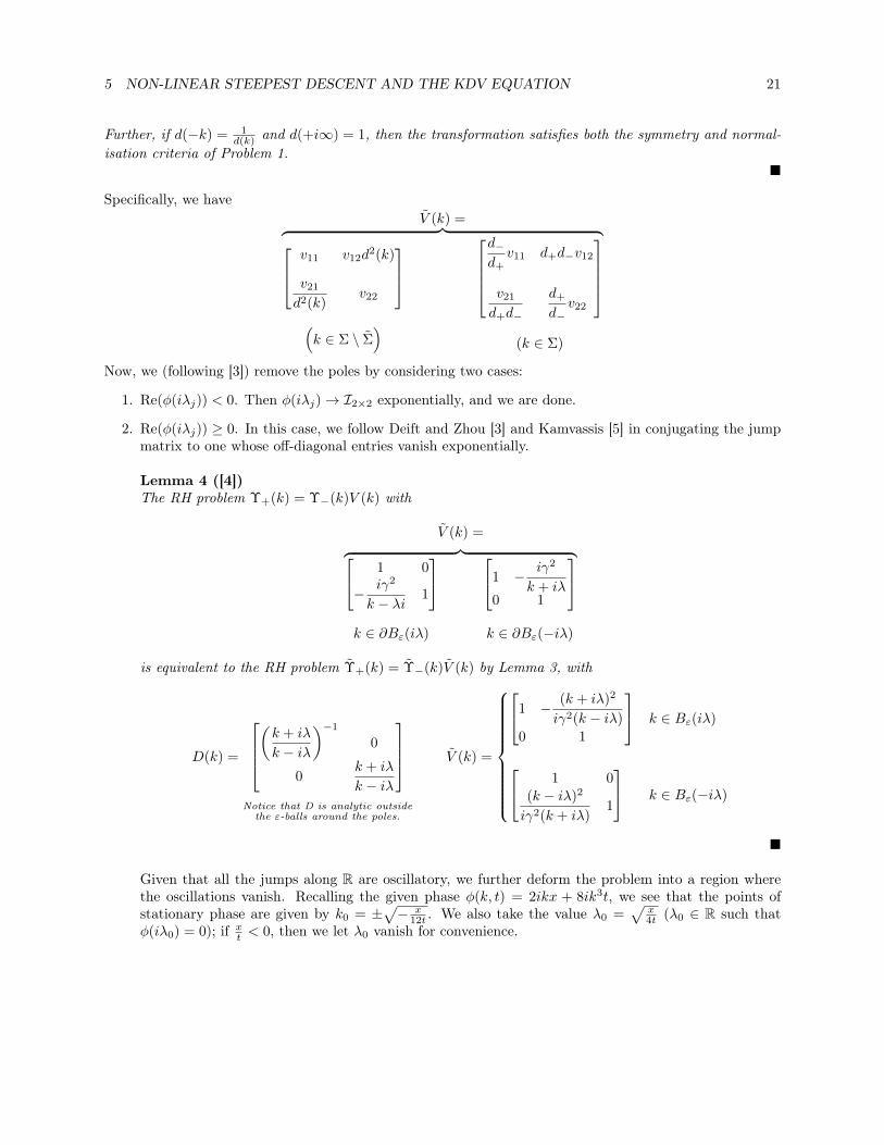
Further, if d(−k) = 1d(k) and d(+i∞) = 1, then the transformation satisfies both the symmetry and normal-

isation criteria of Problem 1.�

Specifically, we haveV (k) =︷︸︸︷ v11 v12d

2(k)

v21

d2(k)v22

(k ∈ Σ \ Σ

)

d−d+

v11 d+d−v12

v21

d+d−

d+

d−v22

(k ∈ Σ)

Now, we (following [3]) remove the poles by considering two cases:

1. Re(φ(iλj)) < 0. Then φ(iλj)→ I2×2 exponentially, and we are done.

2. Re(φ(iλj)) ≥ 0. In this case, we follow Deift and Zhou [3] and Kamvassis [5] in conjugating the jumpmatrix to one whose off-diagonal entries vanish exponentially.

Lemma 4 ([4])The RH problem Υ+(k) = Υ−(k)V (k) with

V (k) =︷︸︸︷ 1 0

− iγ2

k − λi1

k ∈ ∂Bε(iλ)

1 − iγ2

k + iλ0 1

k ∈ ∂Bε(−iλ)

is equivalent to the RH problem Υ+(k) = Υ−(k)V (k) by Lemma 3, with

D(k) =

(k + iλ

k − iλ

)−1

0

0k + iλ

k − iλ

Notice that D is analytic outside

the ε-balls around the poles.

V (k) =

1 − (k + iλ)2

iγ2(k − iλ)

0 1

k ∈ Bε(iλ)

1 0(k − iλ)2

iγ2(k + iλ)1

k ∈ Bε(−iλ)

�

Given that all the jumps along R are oscillatory, we further deform the problem into a region wherethe oscillations vanish. Recalling the given phase φ(k, t) = 2ikx + 8ik3t, we see that the points ofstationary phase are given by k0 = ±

√− x

12t . We also take the value λ0 =√

x4t (λ0 ∈ R such that

φ(iλ0) = 0); if xt < 0, then we let λ0 vanish for convenience.


Factorise V (k) as follows:

V (k) =

[1 R(k)eφ(k,t)

0 1

]︸︷︷︸

b−(k)

−1 [1 0

R(k)eφ(k,t) 1

]︸︷︷︸

b+(k)

|k| > Re(λ0)

[1 0

−R(k)eφ(k,t)

1−|R(k)|

]︸︷︷︸

B−(k)

−1 [1− |R(k)|2 0

0 11−|R(k)|

]︸︷︷︸

A

[1 −R(k)e−φ(k,t)

1−|R(k)|0 1

]︸︷︷︸

B+(k)

|k| < Re(λ0)

Now we eliminate the terms introduced by matrix A in the above factorisation, and conjugate thejumps near the eigenvalues, by defining the partial transmission coefficient with respect to k0 as

T (k, k0) =

∏λj>λ0

(k + iλjk − iλj

)x

t> 0

n∏j=1

(k + iλjk − iλj

)exp

(1

2πi

∫ k0

−k0

ln |T (ξ)|2

ξ − kdξ

)x

t< 0

meromorphic for k ∈ C\Σ(λ0), with k ∈ C\Σ(k0) and Σ(k0) = ∂BRe(k0) (with left-to-right orientation).Taking an O

(1k2

)expansion of the coefficient around k = 0, we get that

T1(k0) =

∑λj>λ0

2λjx

t> 0

n∑j=1

2λj +1

2π

∫ k0

−k0ln(|T (ξ)|2

)dξ

x

t< 0

forT (k, k0) = 1 + T1(k0)i

1

k+O

(1

k2

)(5.5)

Also, we have the following properties ([4]):

(a) T+(k, k0) ≡ (1− |R(k)|2) · T−(k, k0) ∀k ∈ Σ(k0)

(b) T (−k, k0) · T (k, k0) ≡ 1 ∀k ∈ C \ Σ(k0)

(c) T (−k, k0) ≡ T (k, k0) ∀k ∈ C


As in [3] and [4], we define F (k) =

1

T (k, k0)0

0 T (k, k0)

, and create the transformation

D(k) =︷︸︸︷ 1 − k − iλjiγ2j eφ(iλj ,t)

iγ2j eφ(iλj ,t)

k − iλj0

· F (k)

k ∈ Bε(iλj) and λ0 < λj

0 −iγ2j eφ(iλj ,t)

k + iλjk + iλj

iγ2j eφ(iλj ,t)

1

· F (k)

k ∈ Bε(−iλj) and λ0 < λj

F (k)

else

Simplifying, we have that

D(k) =

1

T (k, k0)− (k − iλj)T (k, k0)

iγ2j eφ(iλj ,t)

iγ2j eφ(iλj ,t)

(k − iλj)T (k, k0)0

k ∈ Bε(iλj) and λ0 < λj

0 −

iγ2j eφ(iλj ,t)T (k, k0)

k + iλj

k + iλjiγ2j eφ(iλj ,t)T (k, k0)

T (k, k0)

k ∈ Bε(−iλj) and λ0 < λj

1

T (k, k0)0

0 T (k, k0)

else

(5.6)

We transform the Riemann-Hilbert problem Υ(k) = Υ(k)D(k), where

D(−k) =

[0 11 0

]D(k)

[0 11 0

]


Using Lemmas 3 and 4, we can formulate the jump by

V (k) =

1 − (k − iλj)T 2(k, k0)

iλ2jeφ(iλj ,t)

0 1

k ∈ ∂Bε(iλj)

1 0

− (k + iλj)T2(k, k0)

iγ2j eφ(iλj ,t)

1

k ∈ ∂Bε(−iλj)

λ0 < λj

1 0

−iγ2j eφ(iλj ,t)

(k − iλj)T 2(k, k0)1

k ∈ ∂Bε(iλj)

1 −iλ2jeφ(iλj ,t)

(k + iλj)T 2(k, k0)

0 1

k ∈ ∂Bε(−iλj)

λ0 > λj

Now, all the jumps near singularities will approach I2×2 as t→ +∞ when λ0 6= λj . If λj = λ0, then weretain a pole condition resembling that in Problem 1, but this time compensating for the introductionof the partial transmission coefficient to our new problem:

Res[Υ(k), iλj

]=γ2j eφ(iλj ,t)

T 2(k, k0)limk→iλj

Υ(k)

[0 0i 0

]with the other residue given by the symmetry criterion. The jump along R is then

V (k) =

1R(−k)e−φ(k,t)

T 2(k, k0)

0 1

︸︷︷︸

b−(k)

−1 1 0

R(k)eψ(k,t)

T 2(k, k0)0

︸︷︷︸

b+(k)

k ∈ R \ Σ(k0)

1 0

−T−(k, k0)R(k)eψ(k,t)

T−(k, k0)1

︸︷︷︸

B−(k)

−1 1 −T+(k, k0)R(−k)e−ψ(k,t)

T+(−k, k0)

0 1

︸︷︷︸

B+(k)

k ∈ Σ(k0)

Finally, we deform the jump along R in a way that allows all the oscillatory terms to vanish. Grunertconsiders two cases:

(a) Ifx

t> 0, we take ε > 0 sufficiently small that

i. Σ± = {k ∈ C : Im = ±ε} ⊆ {k : ±Re(φ(k)) < 0}


ii. Bε(±iλj) lies outside of the strip |Im(z)| < ε for all 1 ≤ j ≤ n

Finally, redefine the jump by Υ(k) =

Υ(k)b+(k)−1 0 < Im(k) < ε

Υ(k)b−(k)−1 −ε < Im(k) < 0

Υ(k) else

so that it becomes

V (k) =

{b+(k)−1 k ∈ Σ+

b−(k)−1 k ∈ Σ−

}, vanishing along R, and we are done.

(b) Ifx

t< 0, then Grunert deforms the contour Σ± into Σ1

± ∪ Σ2±, where

• Σ1± holds the value ±ε with positive orientation everywhere on |Re φ(k)| > k0, except in a

neighbourhood of ±k0, where it vanishes smoothly• Σ2

± holds the value ±ε with positive orientation everywhere on |Re φ(k)| < k0, except in aneighbourhood of ±k0, where it vanishes smoothly

• The contours Σ1,2± vanish at the same rate

• Bε(±iλj) lies outside of the region between the contours for all 1 ≤ j ≤ nWe then redefine the problem as

Υ(k) =

Υ(k)b±(k)−1 k between R and Σ1

±Υ(k)B±(k)−1 k between R and Σ2

±Υ(k) else

Again, the jump along R vanishes, and we are left with the jump along the contour given by

V (x) =

{b±(k)±1 k ∈ Σ1

±B±(k)±1 k ∈ Σ2

±

Now, all jumps along Σ± \ {±k0} vanish, and we are done.

Finally, we end by describing the asymptotic behaviour of the solution to the KdV equation when sgn(x) =sgn(t).

Theorem 1 (Asymptotic Behaviour in the Soliton Range [4])

Assume∫R

(1 + |x|)L+1|q(x, 0)| dx <∞ for some integer L ≥ 1 and take the velocity 4λ2j = Re(ψ(iλj)) of the

jth soliton. Let ε > 0 be sufficiently small that the collection {Bε(4λ2j )}i≤j≤n ⊆ R+ is pairwise disjoint.

1. Ifx

t∈ Bε(4λ2

j ) for some j, then

−Q+(x, t) =

∫ ∞x

q(y, t) dt = −4

n∑i=j+1

λi

− 4λjγ2j (x, t)

2λj + γ2j (x, t)

+O(t−L

)

and so we have that q(x, t) =−16λ3

jγ2j (x, t)

(2λj + γ2j (x, t))2

+O(t−L

), where

γ2j (x, t) = γ2

j eφ(iλj ,t)

n∏i=j+1

(λi − λjλi + λj

)2


2. Else, ifx

t6∈ Bε(4λ2

j ) for all j, we have that

−Q+(x, t) =

∫ ∞x

q(y, t) dy = −4

∑λj>λ0

λj

+O(t−L

)(recall that λ0 =

√x

4t

), and so q(x, t) = O

(t−L

).

Proof: ([4])If k is sufficiently far from the R, then Υ(k) ≡ Υ(k), so that we can use (5.4), with the matrix D(k) as givenin (5.6). Taking the truncated series expansion of the partial coefficient T (k, k0) as given in (5.5), we get theexpansion

Υ(k) =

(11

)T+Q+(x, t)− 2T1(k0)

2ki

(−11

)T+O

(1

k2

)Recall that all jumps along the contour vanish exponentially, so we have the following:

Definition 3 (The Cauchy Transform [4, 9])Let Σ be a contour, and f ∈ HomL2 (Σ,C). The Cauchy transform is the analytic functionL2(C \ Σ)→ L2(C) given by

Cf(k) =1

2πi

∫Σ

f(s)

s− kds

with boundary values denoted by C± ∈ End[L2(Σ)

]such that C+ ≡ I+C−. These operators can

also be taken from the Plemelj-Sokhotsky formula C± = 12 (iH ± I), where for k ∈ Σ

Hf(k) =1

πPV

∫Σ

f(s)

k − sds

is the Hilbert transform. �

Definition 4 (The Cauchy Operator [4, 9])If f is a vector-valued function Σ → C2, then the Cauchy operator is the integral operator

C[f ](k) =1

2πi

∫Σ

Ξλ(s, k) ds with the kernel

Ξλ(s, k) = diag

[k + iλ

(s− k)(s+ iλ),

k − iλ(s− k)(s− iλ)

]Denote Cωf = C+(fω−) + C−(fω+) ∈ End

[L2(Σ)

]. �

Lemma 5 ([4]) Let Σ be a fixed contour, and choose λ, γ = γT , and νT depending on someparameter t ∈ R such that we satisfy the following criteria:

1. Σ is a finite collection of smooth oriented finite curves on C which self-intersects almostnowhere and only transversally

2. ±iλ 6∈ Σ and ∃ y0 ∈ R+ such that dist (Σ, iR≥y0) > 0

3. Σ is invariant under the negation map, and is oriented so that all sequences converging toΣ also observe this negation


4. The jump matrix ν is non-singular, with the factorisation

ν = b−1− b+ = (I − ω−)

−1(I + ω+)

ω±(−k) =

[0 11 0

]ω∓(k)

[0 11 0

], k ∈ Σ

5. The jump satisfies ‖ω‖∞ = ‖w+‖Lα(Σ) + ‖w−‖Lα(Σ) <∞ for α ∈ {2,∞}

If ‖ωt‖Lα ≤ ρ(t) for α ∈ {2,∞} for some function ρ(t)→ 0 as t→∞, the operator (I −Cωt) ∈End[L2(Σ)] is invertible for sufficiently large t, and the solution Υ(k) of the Riemann-Hilbertproblem satisfying the above criteria differs from the one soliton solution mt

0(k) only by O(ρ(t)),with the error term dependent on dist (k,Σ ∪ {±iλ}). �

Case 1:x

t∈ Bε(4λ2

j ) or k20 ∈ Bε(λ2

j ) for all i ≤ j ≤ nLet us choose γt = 0 and ωt = ω. Now, ω vanishes exponentially for large t, so that we can use Lemma 5 tosay that all the solutions of the Riemann-Hilbert problems differ only by O

(t−L

)for all L ∈ N+. Therefore,

with reference to the two solutions Υ(k) and m0(k), we must have Q+(x, t)− 2T1(k0) ≡ 0. Hence,

Q+(x, t) = 4T1(k0) = −4

∑λj>λ0

λj

+O(t−L

)Case 2:

x

t6∈ Bε(4λ2

j ) or k20 6∈ Bε(λ2

j ) for some i ≤ j ≤ n.Again, choose ωt = ω, but now γt = γj(x, t), with

γj(x, t) ≡γje

12φ(iλj ,t)

T(iλj ,

λj√3i) ≡ γjeφ(iλj ,t)

n∏i=j+1


)

Again, ω vanishes exponentially, so we conclude that the solutions m0 (Lemma 2) and Υ are identical. Thisgives that

Q+(x, t) ≡ 2T1(k0) +4λγ2eφ(iλ,t)

2λ+ γ2eφ(iλ,t)+O

(t−L

)For k close to R, we can follow the same argument, this time constructing the series expansion using (5.3)instead of (5.4), obtaining the above final terms. Writing

Q+(x, t) ≡ −2

2∑λj>λ0

λj −2λγ2eφ(iλ,t)

2λ+ γ2eφ(iλ,t)

+O(t−L

)differentiation with respect to x and algebraic manipulation gives

q(x, t) ∼ −2

n∑j=1

(λ2j

cosh2[λjx− 4λ2

j − τ(j)]) with τ(j) =

1

2ln

γ2j

2λj

n∏i=j+1


)2

This shows that for large t, the solution will always split into a sum of one-solitons.�

REFERENCES 28

References[1] Ablowitz, Mark J., and Athanassios S. Fokas. Complex variables: introduction and applications. Cam-

bridge University Press, 2003.

[2] Deift, P., Venakides, S., Zhou, X.: An extension of the steepest descent method for Riemann-Hilbertproblems: The small dispersion limit of the Korteweg-de Vries (KdV) equation. Proc. Nat. Acad. of Sci.USA. 95: 450–454 (1998)

[3] Deift, P., Zhou, X,: A Steepest Descent Method for Oscillatory Riemann–Hilbert Problems. Asymptoticsfor the MKdV Equation. Annals of Mathematics. 137: 295–368 (1993)

[4] Grunert, K., Teschl, G.: Long-Time Asymptotics for the Korteweg-de Vries Equation via NonlinearSteepest Descent. Math. Phys. Anal. Geom. 12: 287–324 (2009)

[5] Kamvassis, S,: From Stationary Phase to Steepest Descent. arXiv:math-ph/0701033v5 (4 Mar 2008)

[6] Koelink, E.: Scattering Theory (unpublished master’s degree thesis). Radbout Universiteit Nijmegen,The Netherlands. (2008)

[7] Lenells, J.: Matrix Riemann-Hilbert Problems with Jumps across Carleson Contours. arXiv:1401.2506v2[math.CV] (18 Feb 2014)

[8] Olver, S., Trogdon, T.: Nonlinear steepest descent and the numerical solution of Riemann-Hilbert prob-lems. Comm. Pure App. Math. 67: 135–1389 (2014)

[9] Palais, R.: An Introduction to Wave Equations and Solitons. (unpublished) Dept. Math., U.C. Irvine,CA. (2000)

[10] Paulsen, William. Asymptotic analysis and perturbation theory. CRC Press, 2013.

[11] Tanaka, S.: Korteweg -De Vries Equation; Asymptotic Behaviour of Solutions. Publ. RIMS, Kyoto Univ.10: 367–379 (1975)

The Method of Steepest Descent - math.uwaterloo.catbury/documents/academic_works/steepe… ·...

Documents

Transcript of The Method of Steepest Descent - math.uwaterloo.catbury/documents/academic_works/steepe… ·...