The Impact of Cosmology on Quantum Mechanics∗

James B. Hartle†

Department of Physics, University of California,

Santa Barbara, CA 93106-9530 and

Santa Fe Institute, Santa Fe, NM 87501

(Dated: March 6, 2019)

Abstract

When quantum mechanics was developed in the ’20s of the last century another revolution

in physics was just starting. It began with the discovery that the universe is expanding. For

a long time quantum mechanics and cosmology developed independently of one another. Yet

the very discovery of the expansion would eventually draw the two subjects together because it

implied the big bang where quantum mechanics was important for cosmology and for understanding

and predicting our observations of the universe today. Textbook (Copenhagen) formulations of

quantum mechanics are inadequate for cosmology for at least four reasons: 1) They predict the

outcomes of measurements made by observers. But in the very early universe no measurements

were being made and no observers were around to make them. 2) Observers were outside of the

system being measured. But we are interested in a theory of the whole universe where everything,

including observers, are inside. 3) Copenhagen quantum mechanics could not retrodict the past.

But retrodicting the past to understand how the universe began is the main task of cosmology.

4) Copenhagen quantum mechanics required a fixed classical spacetime geometry not least to give

meaning to the time in the Schrodinger equation. But in the very early universe spacetime is

fluctuating quantum mechanically (quantum gravity) and without definite value. A formulation of

quantum mechanics general enough for cosmology was started by Everett and developed by many.

That effort has given us a more general framework that is adequate for cosmology — decoherent (or

consistent) histories quantum theory in the context of semiclassical quantum gravity. Copenhagen

quantum theory is an approximation to this more general quantum framework that is appropriate

for measurement situations. We discuss whether further generalization may still be required.

∗ A pedagogical essay. Based in part on a talk given at the conference 90 Years of Quantum Mechanics.

Singapore, January, 2017†Electronic address: hartle@physics.ucsb.edu

1

arX

iv:1

901.

0393

3v2

[gr

-qc]

5 M

ar 2

019

Contents

I. Introduction 3

II. The Copenhagen Quantum Mechanics of Laboratory Measurements

(CQM) 4

III. Copenhagen Quantum Mechanics is Inadequate for Cosmology 5

A. No Quasiclassical Realm, No observers, No measurements,

in the Early Universe 6

B. Observers are Physical Systems within the Universe 6

C. No Retrodiction 7

D. Fixed Classical Spacetime 7

IV. A Model Quantum Universe in a Closed Box 8

A. Coarse-grained Histories in General 9

B. Coarse Grained Histories of the Universe 10

V. Decoherent Histories Quantum Theory (DH) 10

A. Two-Slit Experiment 12

B. Calculating Amplitudes for Histories in the Two-Slit Experiment 14

C. A Simple Model of Decoherence 15

D. General Features of Quantum Mechanics Illustrated by the

Two-Slit Experiment 18

VI. Generalized Decoherent Histories Quantum Mechanics of Quantum

Spacetime (GDH) 18

VII. Back to Observations, Measurements, Observers and Copenhagen

Quantum Mechanics as an Approximation. 20

A. Predicting Probabilities for the Results of Observations 20

B. Copenhagen Quantum Mechanics Recovered as an Approximation 20

VIII. Emergent Formulations of Quantum Mechanics for Cosmology 21

IX. Conclusion — Are We Finished Generalizing Quantum Mechanics? 23

2

Acknowledgments 24

References 25

I. INTRODUCTION

In the late ’20s and early ’30s of the last century quantum mechanics was revolutionizing

our understanding of the physics of the very small. At roughly the same time another

revolution in physics was beginning that was to change our understanding of the physics of

the very large. This started with the discovery that the universe was expanding through

the work of Lemaıtre, Hubble, and Slipher. For many years these two revolutions proceeded

independently of one another. But in more recent times each has had a significant impact

on the other.

Quantum mechanics is central to an understanding of important physical processes that

take place in the very early universe. Well known examples are big bang nucleosynthesis,

recombination, and, most importantly, the generation of quantum fluctuations in matter

density that grow under gravitational attraction to produce the large scale structure we see

today in the distribution of the galaxies and in the temperature fluctuations of the cosmic

background radiation (CMB).

What is perhaps less widely appreciated that cosmology had a significant impact on

our understanding of quantum mechanics. That is because the Copenhagen formulations

that appear in many textbooks are inadequate for cosmology for several reasons. Quantum

mechanics had to be generalized to apply to cosmology, and those generalizations led to a

different understanding of the subject and what it is about.

This essay will describe very briefly the impact of cosmology on quantum mechanics and

a little of the more general formulations of quantum theory that resulted. Throughout we

attempt to explain the basic ideas with a minimum of technical development.1 We trade

lack of precision for hope of being more widely understandable.

We should also stress that we will not address issues of the interpretation of quantum

theory. Rather, we aim at describing how cosmology has affected what has to be interpreted.

1 That is with a minimum of equations. For those who want the equations there are a large number of

references, many by the author, that offer different levels of explanation.

3

We begin in Section II by describing the status of Copenhagen quantum mechanics (CQM)

today. Section III explains why this Copenhagen quantum theory is inadequate for cos-

mology and why a generalization of it is needed. Section IV describes a model quantum

universe in a very large box. Section V describes the decoherent (or consistent) histories

generalization of Copenhagen quantum theory that is adequate for closed systems like the

universe. Section VI describes further generalizations to deal with quantum spacetime ge-

ometry. Section VII A describes how to get probabilities for the results of our observations

from probabilities for histories of the universe. Section VII B recovers Copenhagen quantum

mechanics as approximation appropriate for measurement situations in more general formu-

lations of quantum mechanics applicable to the universe. Section VIII describes how various

formulations of quantum theory can be regarded as features of the universe that emerge

along with other features that are a prerequisite to the formulations. Section Section IX

concludes by speculating on whether further generalizations will be required .

II. THE COPENHAGEN QUANTUM MECHANICS OF LABORATORY MEA-

SUREMENTS (CQM)

The Copenhagen quantum mechanics (CQM) found in standard textbooks2 is arguably

the most successful theoretical framework in the history of physics. It is central to our

understanding of a vast range of physical phenomena, including atoms, molecules, chemistry,

the solid state, how stars are formed, shine, evolve, and die, nuclear energy, thermonuclear

explosions, how transistors work, and many, many, many, more phenomena. It has often

been claimed that quantum mechanics is responsible for a significant fraction of the US

GDP.

Work continues today to better understand Copenhagen quantum mechanics, to make

its central notions of measurement and state vector reduction more precise, and to resolve

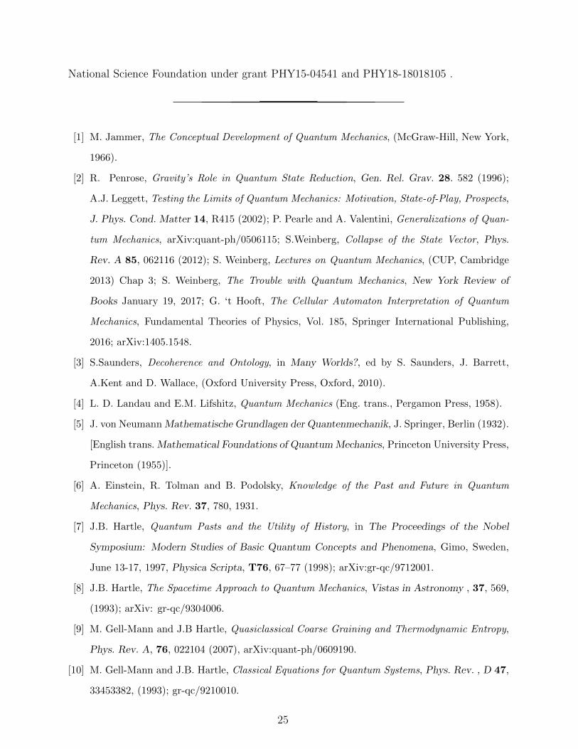
‘problems’ that it is alleged to have like the ‘measurement problem’ (Figure 1). Even given

these concerns, the author knows no mistake that was made because of them in correctly

2 By ‘Copenhagen quantum mechanics’, or ‘textbook quantum mechanics’ we mean the standard formula-

tion that is found in many textbooks including the assumption of the quasiclassical realm of every day

experience as described in III A. We do not necessarily mean that it conforms exactly to what the founders

of quantum mechanics meant by the ‘Copenhagen interpretation of quantum mechanics’ [1].

4

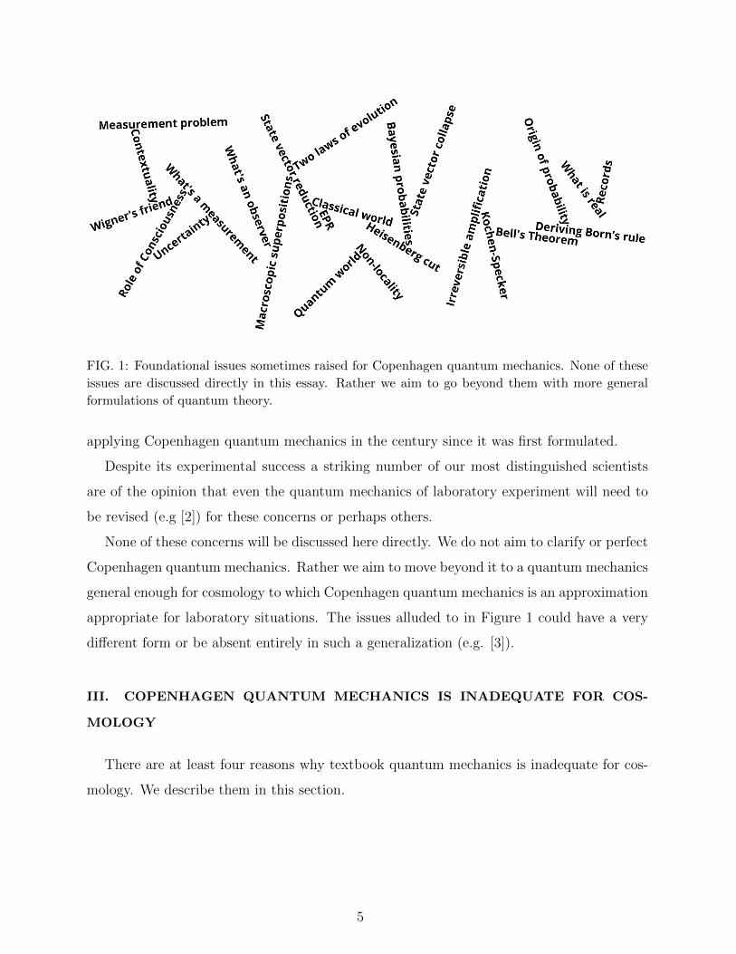
FIG. 1: Foundational issues sometimes raised for Copenhagen quantum mechanics. None of these

issues are discussed directly in this essay. Rather we aim to go beyond them with more general

formulations of quantum theory.

applying Copenhagen quantum mechanics in the century since it was first formulated.

Despite its experimental success a striking number of our most distinguished scientists

are of the opinion that even the quantum mechanics of laboratory experiment will need to

be revised (e.g [2]) for these concerns or perhaps others.

None of these concerns will be discussed here directly. We do not aim to clarify or perfect

Copenhagen quantum mechanics. Rather we aim to move beyond it to a quantum mechanics

general enough for cosmology to which Copenhagen quantum mechanics is an approximation

appropriate for laboratory situations. The issues alluded to in Figure 1 could have a very

different form or be absent entirely in such a generalization (e.g. [3]).

III. COPENHAGEN QUANTUM MECHANICS IS INADEQUATE FOR COS-

MOLOGY

There are at least four reasons why textbook quantum mechanics is inadequate for cos-

mology. We describe them in this section.

5

A. No Quasiclassical Realm, No observers, No measurements,

in the Early Universe

Copenhagen quantum mechanics assumes the quasiclassical realm of every day experience

— the wide range of time, place, and scale on which the deterministic laws of classical physics

apply. Notable examples are the laws of gravity summarized by the Einstein equation and

the laws of motion of continua summarized in the Navier-Stokes equation. These and other

classical laws are needed just to describe measurement apparatus and observers and their

operation in physical terms. Indeed, some formulations of Copenhagen quantum mechanics

assumed the existence entirely separate classical and quantum worlds with a kind of movable

boundary between them (e.g. [4]). There is no evidence for such a division in cosmology.

B. Observers are Physical Systems within the Universe

Copenhagen quantum mechanics predicts probabilities for the outcomes of measurements

carried out on a subsystem of the universe by another subsystem called the ‘observer’ or

‘measuring apparatus’ that is outside the subsystem being measured3.

But in the very early universe there were no measurements being made and no observers

around to make them. Are we to believe that quantum mechanics does not apply to the

early universe before the evolution of observers approximately 10 Gyr after the big bang?

Certainly not! But then we need a generalization of Copenhagen quantum mechanics in

which observers are physical systems inside the universe. We need a generalization of text-

book quantum mechanics in which observers and their measurements can be described in

quantum mechanical terms but play no special role in the theory’s formulation and are not

prerequisites for the theory’s application4.

3 Individually and collectively observers are examples of the general concept of IGUSes — information

gathering and utilizing subsystems. It would be both more accurate and more accessible to present

Copenhagen quantum mechanics in terms of IGUSes. But we aim at a discussion that is as broadly

accessible as possible and to that end we will stick with the more broadly familiar if less nuanced ‘observer’

in this paper.4 Sometimes one meets the suggestion that no such generalization is needed. The idea is that Copenhagen

quantum mechanics retrodicts the past when present observers measure present records of what went on

in the past. But what exactly is a record? A record is a physical quantity today that is correlated with

one or more past events with high probability. This probability is for a two time history of the events and

6

C. No Retrodiction

In his now classic book The Mathematical Foundations of Quantum Mechanics [5] John

von Neumann formulated quantum evolution in terms of two laws. First, unitary evolution

of the state vector described by the Schrodinger equation. Second, the reduction of the

state vector after an ‘ideal’ measurement5 that disturbs the measured subsystem as little as

possible.

Starting from the state of an isolated subsystem at one time, and using these two laws,

Copenhagen quantum theory can predict probabilities for the histories of later measurements

an observer might decide to carry out on the same subsystem. This is the sense in which

Copenhagen quantum theory can predict the results of future measurements starting from

the present state of the measured subsystem.

Copenhagen quantum mechanics cannot retrodict the past of a subsystem starting from

its present quantum state. The Schrodinger differential equation can of course be evolved

backward in time as well as forward. But state vector reduction runs only one way —

forward in time, usually taken to be the direction in which entropy is increasing in the

universe. Thus retrodiction is impossible in Copenhagen quantum mechanics6.

But retrodiction is central to cosmology. We use present data and and an initial quantum

state to make a model of what went on in our past to simplify our predictions of the future [7].

We are interested in particular in a quantum framework that can can be used to construct a

history of how the universe came to be the way it is today starting from its initial condition

roughly 14Gyr ago using its quantum state.

D. Fixed Classical Spacetime

Copenhagen quantum mechanics assumes a fixed spacetime geometry. This geometry

defines the possible time directions for the ‘t’ in the Schrodinger equation. States are defined

the formation of a later record of them. A generalization of Copenhagen quantum mechanics is needed to

assign probabilities to such time histories and define what is meant by records.5 vonNeumann had the opposite order of one and two but the one here is more used today6 The sole consideration of the past in Copenhagen quantum theory appears to be a paper by Einstein,

Podolsky and Tolman [6] which concluded ‘quantum mechanics must involve an uncertainty in the de-

scription of past events which is analogous to the uncertainty in the prediction of future events’. (Don

Howard, private communication).

7

on spacelike surfaces in this fixed spacetime and evolve by the Schrodinger equation through

a foliating family of such surfaces in this fixed spacetime. After an ideal measurement,

the state is ‘reduced’ all across one of these spacelike surfaces that extend over the whole

universe. Copenhagen quantum mechanics requires a fixed spacetime geometry just to make

sense of these two modes of evolution.

But in the early universe near the big bang energy scales above the Planck scale

(hc5/G)1/2 ∼ 1019Gev will be reached at which quantum gravity becomes important and

spacetime geometry will fluctuate quantum mechanically and be without the definiteness

required by Copenhagen quantum theory.

Rather we expect Copenhagen quantum mechanics to emerge in the early universe along

with classical spacetime geometry when the latter is sufficiently slowly varying to provide

the notions of time and spacelike surfaces that Copenhagen quantum mechanics assumes

(e.g. [8]).

The conclusion of the discussion in this section is that CQM has to be generalized for

quantum cosmology. The rest of the paper discusses possible generalizations.

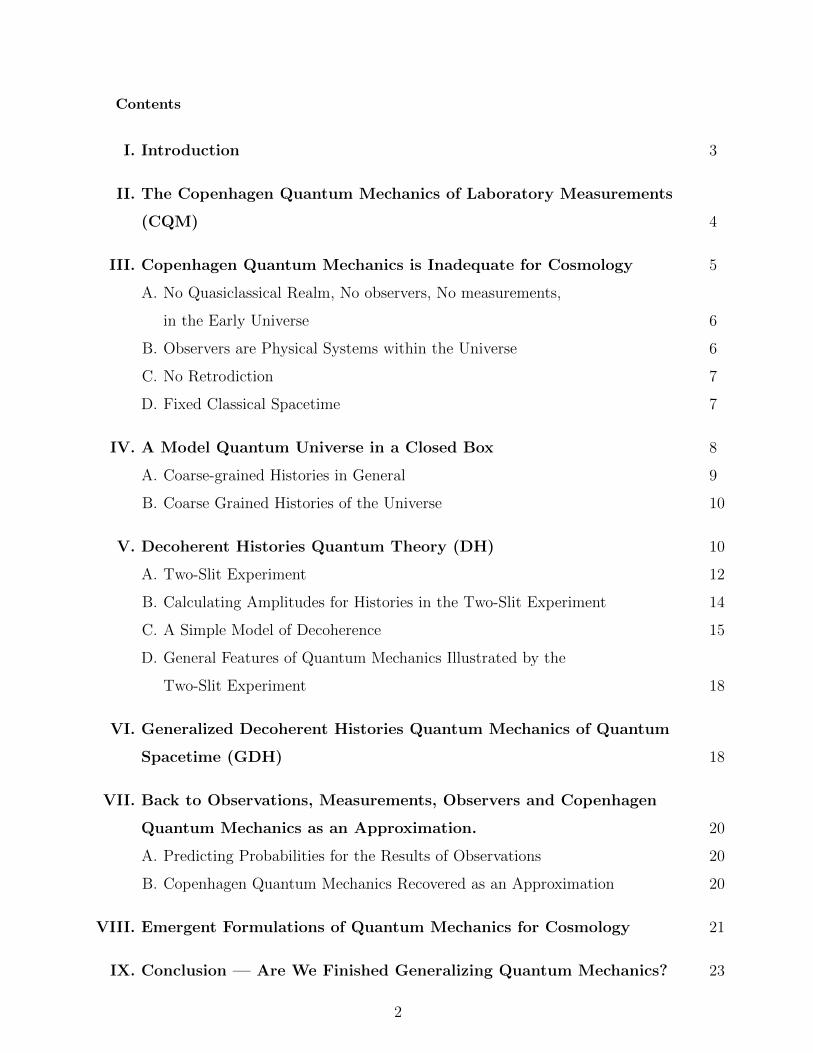
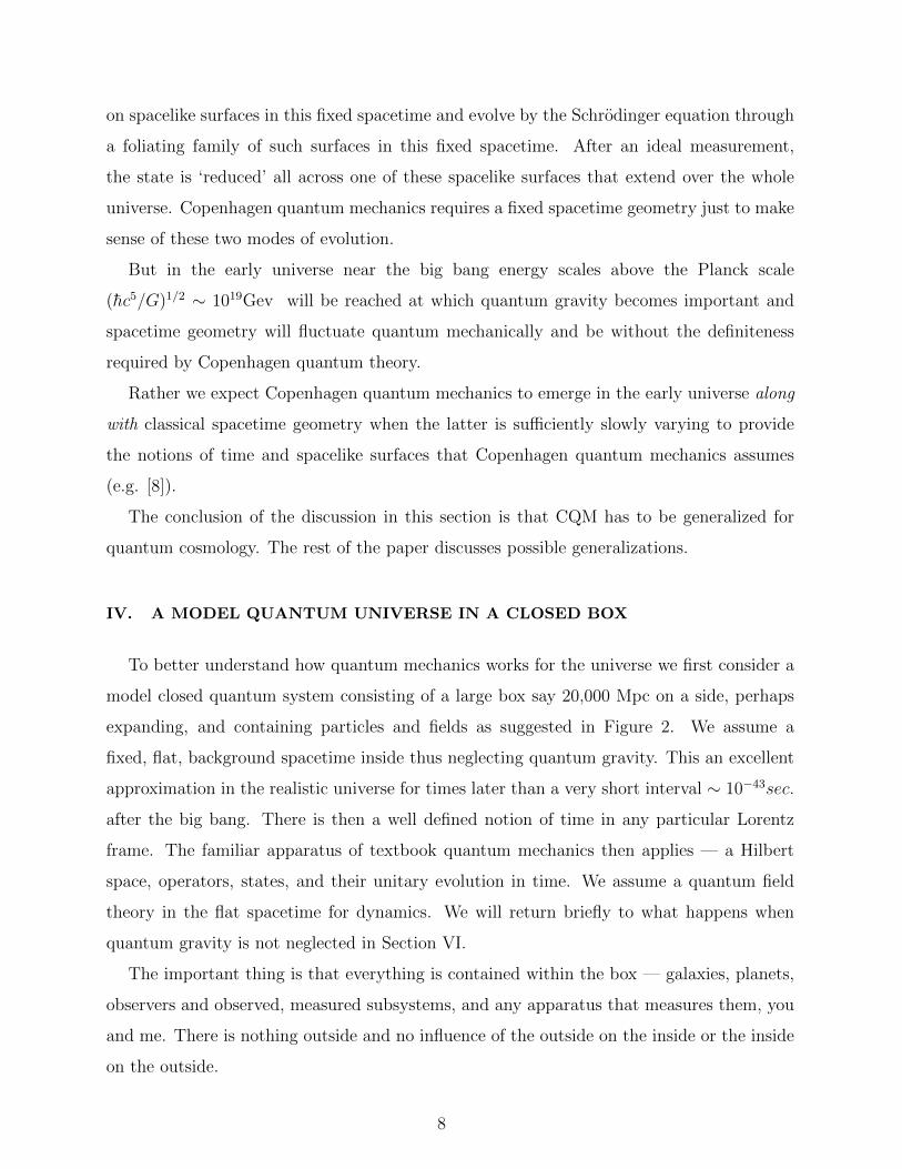
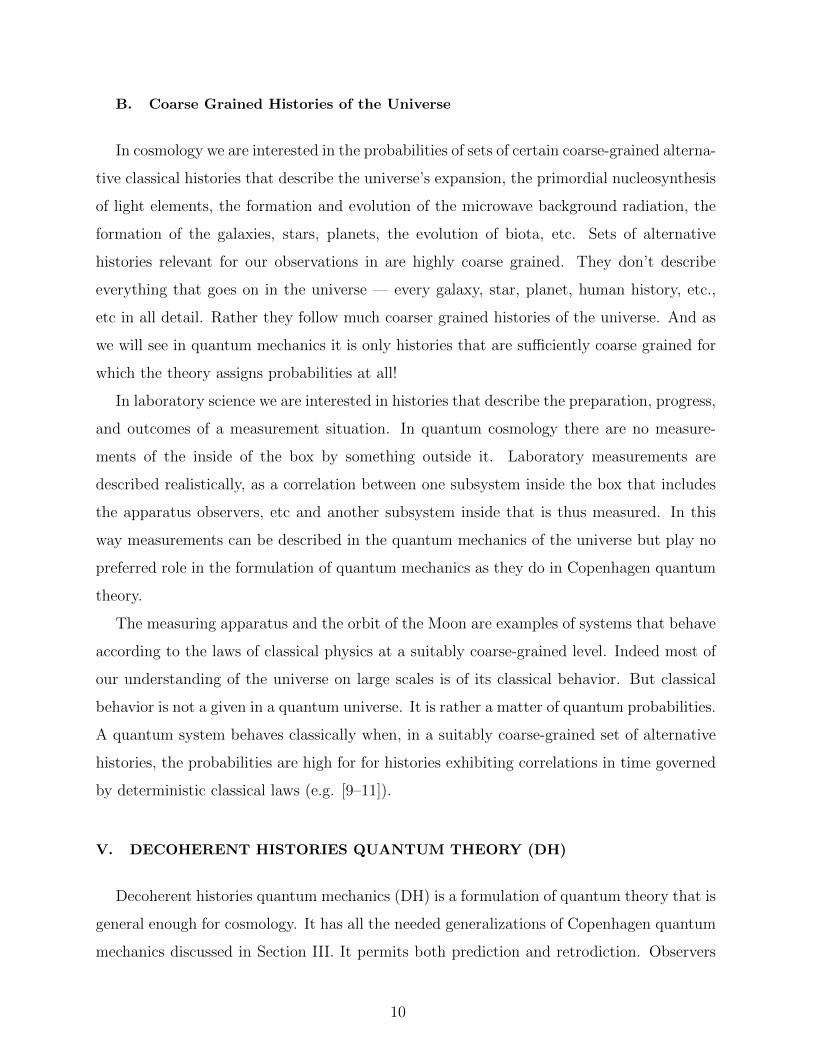
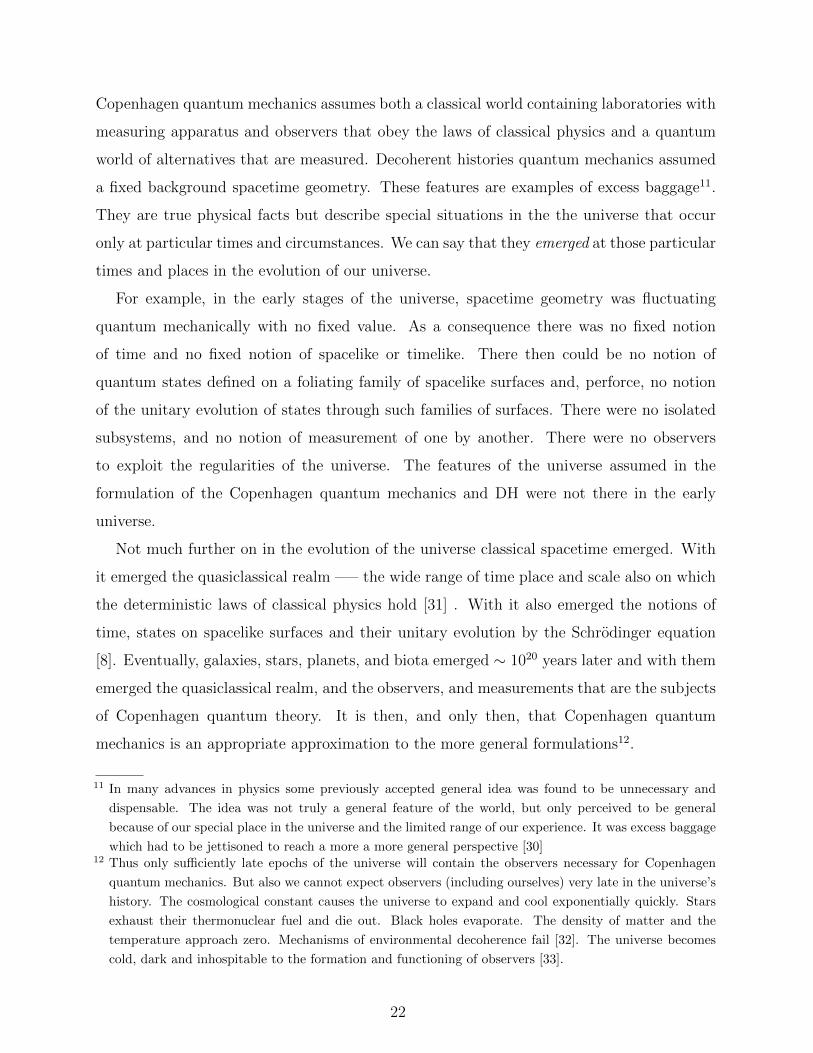
IV. A MODEL QUANTUM UNIVERSE IN A CLOSED BOX

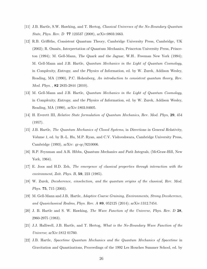
To better understand how quantum mechanics works for the universe we first consider a

model closed quantum system consisting of a large box say 20,000 Mpc on a side, perhaps

expanding, and containing particles and fields as suggested in Figure 2. We assume a

fixed, flat, background spacetime inside thus neglecting quantum gravity. This an excellent

approximation in the realistic universe for times later than a very short interval ∼ 10−43sec.

after the big bang. There is then a well defined notion of time in any particular Lorentz

frame. The familiar apparatus of textbook quantum mechanics then applies — a Hilbert

space, operators, states, and their unitary evolution in time. We assume a quantum field

theory in the flat spacetime for dynamics. We will return briefly to what happens when

quantum gravity is not neglected in Section VI.

The important thing is that everything is contained within the box — galaxies, planets,

observers and observed, measured subsystems, and any apparatus that measures them, you

and me. There is nothing outside and no influence of the outside on the inside or the inside

on the outside.

8

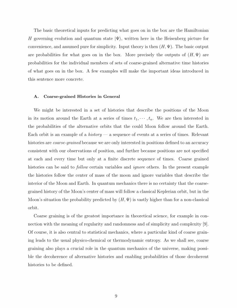
The basic theoretical inputs for predicting what goes on in the box are the Hamiltonian

H governing evolution and quantum state |Ψ〉, written here in the Heisenberg picture for

convenience, and assumed pure for simplicity. Input theory is then (H,Ψ). The basic output

are probabilities for what goes on in the box. More precisely the outputs of (H,Ψ) are

probabilities for the individual members of sets of coarse-grained alternative time histories

of what goes on in the box. A few examples will make the important ideas introduced in

this sentence more concrete.

A. Coarse-grained Histories in General

We might be interested in a set of histories that describe the positions of the Moon

in its motion around the Earth at a series of times t1, · · · , tn. We are then interested in

the probabilities of the alternative orbits that the could Moon follow around the Earth.

Each orbit is an example of a history — a sequence of events at a series of times. Relevant

histories are coarse-grained because we are only interested in positions defined to an accuracy

consistent with our observations of position, and further because positions are not specified

at each and every time but only at a finite discrete sequence of times. Coarse grained

histories can be said to follow certain variables and ignore others. In the present example

the histories follow the center of mass of the moon and ignore variables that describe the

interior of the Moon and Earth. In quantum mechanics there is no certainty that the coarse-

grained history of the Moon’s center of mass will follow a classical Keplerian orbit, but in the

Moon’s situation the probability predicted by (H,Ψ) is vastly higher than for a non-classical

orbit.

Coarse graining is of the greatest importance in theoretical science, for example in con-

nection with the meaning of regularity and randomness and of simplicity and complexity [9].

Of course, it is also central to statistical mechanics, where a particular kind of coarse grain-

ing leads to the usual physico-chemical or thermodynamic entropy. As we shall see, coarse

graining also plays a crucial role in the quantum mechanics of the universe, making possi-

ble the decoherence of alternative histories and enabling probabilities of those decoherent

histories to be defined.

9

B. Coarse Grained Histories of the Universe

In cosmology we are interested in the probabilities of sets of certain coarse-grained alterna-

tive classical histories that describe the universe’s expansion, the primordial nucleosynthesis

of light elements, the formation and evolution of the microwave background radiation, the

formation of the galaxies, stars, planets, the evolution of biota, etc. Sets of alternative

histories relevant for our observations in are highly coarse grained. They don’t describe

everything that goes on in the universe — every galaxy, star, planet, human history, etc.,

etc in all detail. Rather they follow much coarser grained histories of the universe. And as

we will see in quantum mechanics it is only histories that are sufficiently coarse grained for

which the theory assigns probabilities at all!

In laboratory science we are interested in histories that describe the preparation, progress,

and outcomes of a measurement situation. In quantum cosmology there are no measure-

ments of the inside of the box by something outside it. Laboratory measurements are

described realistically, as a correlation between one subsystem inside the box that includes

the apparatus observers, etc and another subsystem inside that is thus measured. In this

way measurements can be described in the quantum mechanics of the universe but play no

preferred role in the formulation of quantum mechanics as they do in Copenhagen quantum

theory.

The measuring apparatus and the orbit of the Moon are examples of systems that behave

according to the laws of classical physics at a suitably coarse-grained level. Indeed most of

our understanding of the universe on large scales is of its classical behavior. But classical

behavior is not a given in a quantum universe. It is rather a matter of quantum probabilities.

A quantum system behaves classically when, in a suitably coarse-grained set of alternative

histories, the probabilities are high for for histories exhibiting correlations in time governed

by deterministic classical laws (e.g. [9–11]).

V. DECOHERENT HISTORIES QUANTUM THEORY (DH)

Decoherent histories quantum mechanics (DH) is a formulation of quantum theory that is

general enough for cosmology. It has all the needed generalizations of Copenhagen quantum

mechanics discussed in Section III. It permits both prediction and retrodiction. Observers

10

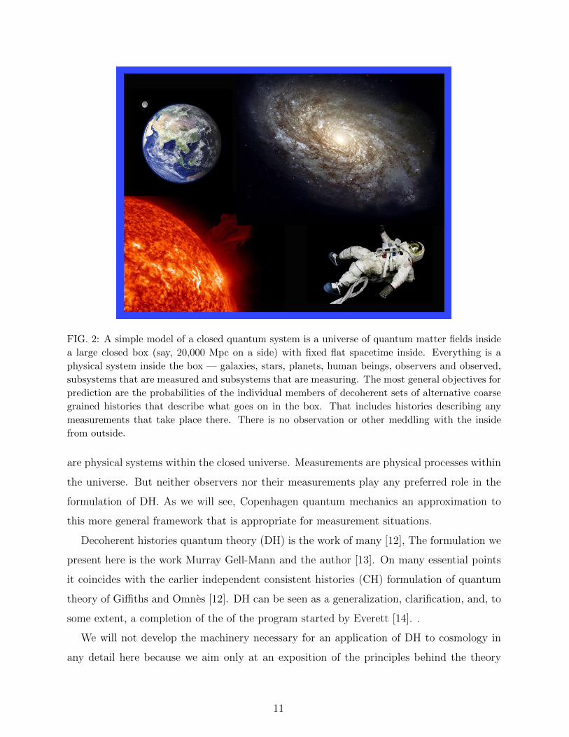
FIG. 2: A simple model of a closed quantum system is a universe of quantum matter fields inside

a large closed box (say, 20,000 Mpc on a side) with fixed flat spacetime inside. Everything is a

physical system inside the box — galaxies, stars, planets, human beings, observers and observed,

subsystems that are measured and subsystems that are measuring. The most general objectives for

prediction are the probabilities of the individual members of decoherent sets of alternative coarse

grained histories that describe what goes on in the box. That includes histories describing any

measurements that take place there. There is no observation or other meddling with the inside

from outside.

are physical systems within the closed universe. Measurements are physical processes within

the universe. But neither observers nor their measurements play any preferred role in the

formulation of DH. As we will see, Copenhagen quantum mechanics an approximation to

this more general framework that is appropriate for measurement situations.

Decoherent histories quantum theory (DH) is the work of many [12], The formulation we

present here is the work Murray Gell-Mann and the author [13]. On many essential points

it coincides with the earlier independent consistent histories (CH) formulation of quantum

theory of Giffiths and Omnes [12]. DH can be seen as a generalization, clarification, and, to

some extent, a completion of the of the program started by Everett [14]. .

We will not develop the machinery necessary for an application of DH to cosmology in

any detail here because we aim only at an exposition of the principles behind the theory

11

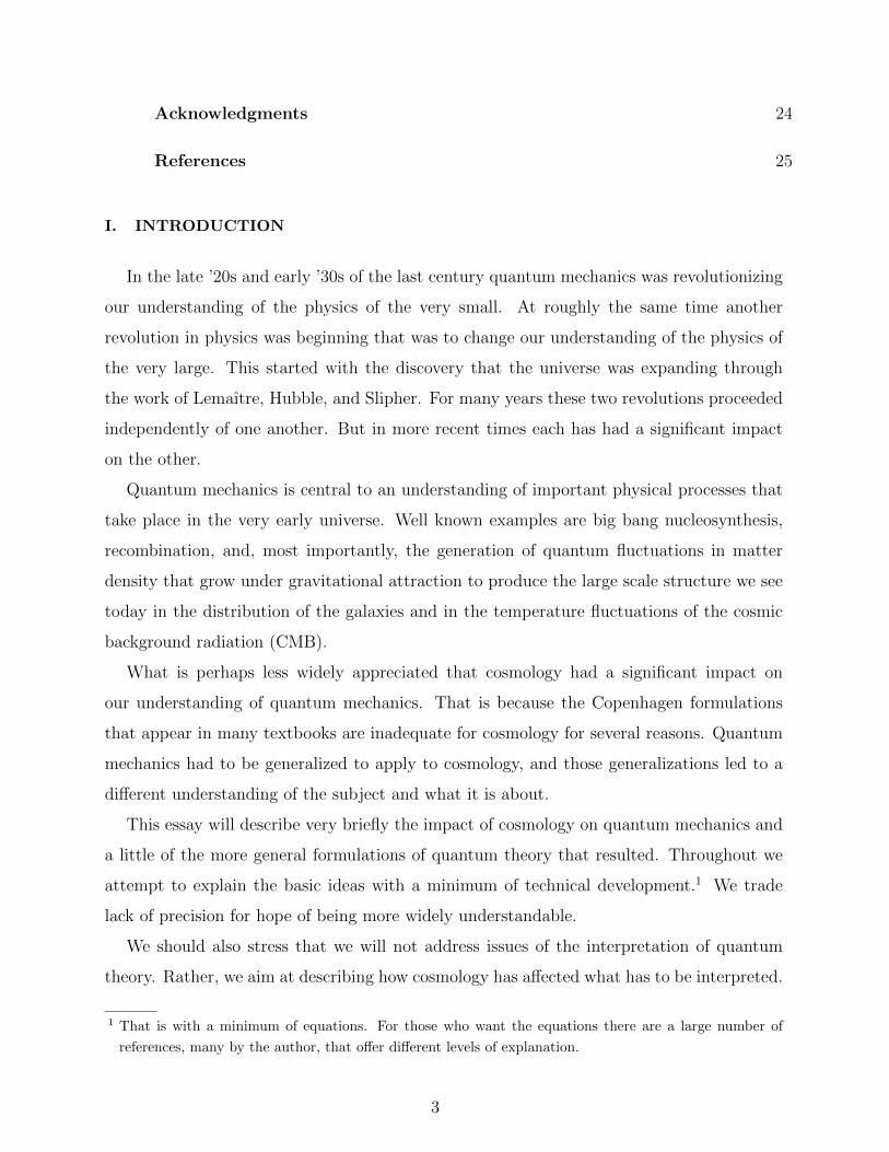
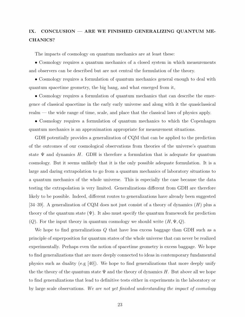
2Ψ

U

L

y

y

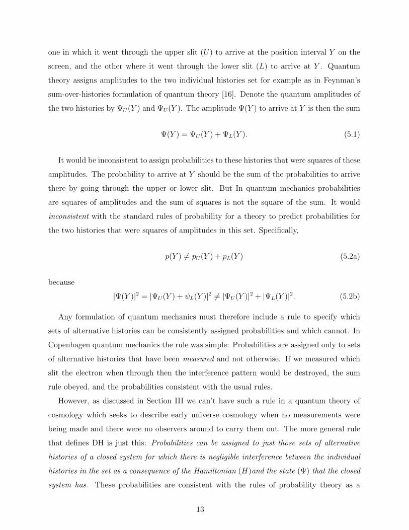
FIG. 3: The two-slit experiment. An electron gun at left emits an electron traveling towards

a screen with two slits, its progress in space recapitulating its evolution in time. When precise

detections are made of an ensemble of such electrons at the screen the classic interference pattern

emerges — evidence that the two histories interfere. is not possible, because of this quantum

interference, to assign a probability to the alternatives of whether an individual electron went

through the upper slit or the lower slit. However, if the electron interacts with apparatus that

measures which slit it passed through, then these alternatives decohere and probabilities can be

assigned.

with a minimum of technical complication7. For definiteness we first focus this discussion

on the universe in a box of the previous section with a fixed, flat, spacetime geometry. As

described there, we aim at predicting probabilities for the individual members of sets of

coarse grained alternative histories of what goes on in the box. But quantum interference

is an obstacle to assigning probabilities sets of alternative histories for any closed system.

Nowhere is this more simply illustrated than in the classic two-slit experiment shown in Fig.

3.

A. Two-Slit Experiment

In the two-slit setup shown in Figure 3 suppose an electron arrives at a position Y on

the detecting screen after passing through a screen with two slits U and L. There is an

obvious set of two alternative histories of how it might have got to the detecting screen —

7 For a pedagogical introduction with more equations than here see, e.g. [15].

12

one in which it went through the upper slit (U) to arrive at the position interval Y on the

screen, and the other where it went through the lower slit (L) to arrive at Y . Quantum

theory assigns amplitudes to the two individual histories set for example as in Feynman’s

sum-over-histories formulation of quantum theory [16]. Denote the quantum amplitudes of

the two histories by ΨU(Y ) and ΨU(Y ). The amplitude Ψ(Y ) to arrive at Y is then the sum

Ψ(Y ) = ΨU(Y ) + ΨL(Y ). (5.1)

It would be inconsistent to assign probabilities to these histories that were squares of these

amplitudes. The probability to arrive at Y should be the sum of the probabilities to arrive

there by going through the upper or lower slit. But In quantum mechanics probabilities

are squares of amplitudes and the sum of squares is not the square of the sum. It would

inconsistent with the standard rules of probability for a theory to predict probabilities for

the two histories that were squares of amplitudes in this set. Specifically,

p(Y ) 6= pU(Y ) + pL(Y ) (5.2a)

because

|Ψ(Y )|2 = |ΨU(Y ) + ψL(Y )|2 6= |ΨU(Y )|2 + |ΨL(Y )|2. (5.2b)

Any formulation of quantum mechanics must therefore include a rule to specify which

sets of alternative histories can be consistently assigned probabilities and which cannot. In

Copenhagen quantum mechanics the rule was simple: Probabilities are assigned only to sets

of alternative histories that have been measured and not otherwise. If we measured which

slit the electron when through then the interference pattern would be destroyed, the sum

rule obeyed, and the probabilities consistent with the usual rules.

However, as discussed in Section III we can’t have such a rule in a quantum theory of

cosmology which seeks to describe early universe cosmology when no measurements were

being made and there were no observers around to carry them out. The more general rule

that defines DH is just this: Probabilities can be assigned to just those sets of alternative

histories of a closed system for which there is negligible interference between the individual

histories in the set as a consequence of the Hamiltonian (H)and the state (Ψ) that the closed

system has. These probabilities are consistent with the rules of probability theory as a

13

result of the absence of quantum interference. Such a set of histories for which the mutual

interference between any pair of histories is negligible is said to decohere.

B. Calculating Amplitudes for Histories in the Two-Slit Experiment

We can get an idea of how to calculate the amplitudes for histories in the two-slit exper-

iment just from the Schrodinger equation defining the quantum evolution of the electron’s

wave function. To keep the discussion simple we ignore the spin of the electron and consider

only its position. The state of the electron in the two-slit experiment can then be described

by a wave function of the form

Ψ = Ψ(x, y, t) (5.3)

using a coordinate x for the horizontal direction and y for the vertical direction in Figure 3

and assuming symmetry in the perpendicular direction.

Denote the initial state at time t0 by Ψ(x, y, t0). This is a product of wave packet in the

x-direction φ(x, t0) and a wave function ψ0(y, t0) localized at the gun, viz.

Ψ(x, y, t0) = ψ(y, t0)φ(x, t0). (5.4)

This wave function evolves in time by the Schrodinger equation

ih∂Ψ

∂t= HΨ. (5.5)

where H is the Hamiltonian of a free particle interacting with the screens. We assume that

φ(x, t) is a narrow wave packet peaked to the left of the slits but moving to the right so as to

reach the slits at time ts and the detecting screen at td. Thus, its progress in x recapitulates

evolution in time. After passing through the slits the wave function has the approximate

form

Ψ(x, y, t) = ψU(y, t)φ(x, t) + ΨL(y, t)φ(x, t), ts < t < td. (5.6a)

≡ ΨU(x, y, t) + ΨL(x, y, t). (5.6b)

Here, in the first term, ψU(y, t) is localized near the upper slit at time ts and spreads over

14

a larger region of y by the time td that the wave packet hits the detecting screen. Similarly

for the second term. When evaluated at the arrival position xd and time td ,and projected

on the interval of arrival Y , these are the amplitudes ΨU(Y ) and ΨL(Y ) in (5.1). They are

wave functions of two branch state vectors |ΨU(Y )〉 and |ΨL(Y )〉 for the two histories in the

set. The set does not decohere because

〈ΨU(Y )|ΨL(Y )〉 6≈ 0 (5.7)

so that the decoherence condition is not satisfied. The two histories interfere. There will be

no consistent set of probabilities for this set of histories .

C. A Simple Model of Decoherence

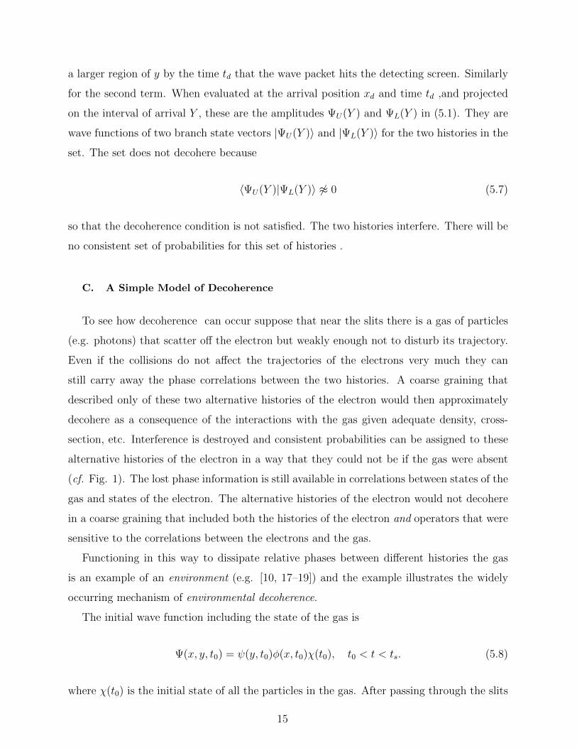
To see how decoherence can occur suppose that near the slits there is a gas of particles

(e.g. photons) that scatter off the electron but weakly enough not to disturb its trajectory.

Even if the collisions do not affect the trajectories of the electrons very much they can

still carry away the phase correlations between the two histories. A coarse graining that

described only of these two alternative histories of the electron would then approximately

decohere as a consequence of the interactions with the gas given adequate density, cross-

section, etc. Interference is destroyed and consistent probabilities can be assigned to these

alternative histories of the electron in a way that they could not be if the gas were absent

(cf. Fig. 1). The lost phase information is still available in correlations between states of the

gas and states of the electron. The alternative histories of the electron would not decohere

in a coarse graining that included both the histories of the electron and operators that were

sensitive to the correlations between the electrons and the gas.

Functioning in this way to dissipate relative phases between different histories the gas

is an example of an environment (e.g. [10, 17–19]) and the example illustrates the widely

occurring mechanism of environmental decoherence.

The initial wave function including the state of the gas is

Ψ(x, y, t0) = ψ(y, t0)φ(x, t0)χ(t0), t0 < t < ts. (5.8)

where χ(t0) is the initial state of all the particles in the gas. After passing through the slits

15

!2

y

FIG. 4: The two-slit experiment with an interacting gas. Near the slits light particles of a gas

collide with the electrons. Even if the collisions do not affect the trajectories of the electrons very

much they can still carry away the phase correlations between the histories in which the electron

arrived at point y on the screen by passing through the upper slit and that in which it arrived at

the same point by passing through the lower slit. A coarse graining that described only of these

two alternative histories of the electron would approximately decohere as a consequence of the

interactions with the gas given adequate density, cross-section, etc. Interference is destroyed and

probabilities can be assigned to these alternative histories of the electron in a way that they could

not be if the gas were not present (cf. Fig. 1). .

this becomes

Ψ(x, y, t) = ψU(y, t)φ(x, t)χU(t) + ψL(y, t)φ(x, t)χL(t), ts < t < td. (5.9a)

≡ ΨU(x, y, t) + ΨL(x, y, t). (5.9b)

where χU(t) and χL(t) denote the state of the gas particles that have scattered from the

region of the upper and lower slit respectively. Then ΨU(x, y, td) and ΨL(x, y, td) are the

branch wave functions for the two histories that the electron arrived in the interval Y at time

td after passing through either the upper or lower slit. The condition that this set of two

histories decoheres is the absence of interference between these two branch wave functions,

16

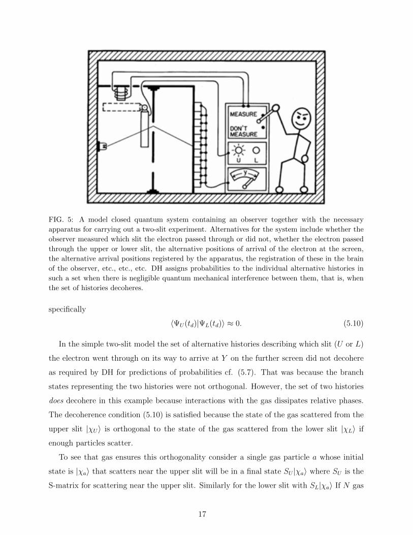
FIG. 5: A model closed quantum system containing an observer together with the necessary

apparatus for carrying out a two-slit experiment. Alternatives for the system include whether the

observer measured which slit the electron passed through or did not, whether the electron passed

through the upper or lower slit, the alternative positions of arrival of the electron at the screen,

the alternative arrival positions registered by the apparatus, the registration of these in the brain

of the observer, etc., etc., etc. DH assigns probabilities to the individual alternative histories in

such a set when there is negligible quantum mechanical interference between them, that is, when

the set of histories decoheres.

specifically

〈ΨU(td)|ΨL(td)〉 ≈ 0. (5.10)

In the simple two-slit model the set of alternative histories describing which slit (U or L)

the electron went through on its way to arrive at Y on the further screen did not decohere

as required by DH for predictions of probabilities cf. (5.7). That was because the branch

states representing the two histories were not orthogonal. However, the set of two histories

does decohere in this example because interactions with the gas dissipates relative phases.

The decoherence condition (5.10) is satisfied because the state of the gas scattered from the

upper slit |χU〉 is orthogonal to the state of the gas scattered from the lower slit |χL〉 if

enough particles scatter.

To see that gas ensures this orthogonality consider a single gas particle a whose initial

state is |χa〉 that scatters near the upper slit will be in a final state SU |χa〉 where SU is the

S-matrix for scattering near the upper slit. Similarly for the lower slit with SL|χa〉 If N gas

17

particles scatter the overlap between |χU〉 and |χL〉 will be proportional to N inner products

of the formN∏a=1

|〈χa|S†USL|χa〉|. (5.11)

Since the two final state vectors SU |χa〉 and SL|χa〉 are different each individual product has

a magnitude less than 1. The product of a very large number of such products will be near

zero implying decoherence as in (5.10).

D. General Features of Quantum Mechanics Illustrated by the

Two-Slit Experiment

This two-slit example illustrates two general features of the quantum mechanics of histo-

ries that are central to its formulation.

First, it illustrates that sets of alternative histories must decohere in order to have prob-

abilities consistent with the rules of probability theory.

Second, the two-slit experiment illustrates the crucial role that coarse graining plays by

making decoherence possible. Sets of fine-grained alternative histories like the set of all

possible Feynman paths of a particle generally do not decohere except in trivial cases. Some

degrees of freedom must be ignored to carry away the phase information between individual

coarse grained histories that can be followed. It is remarkable fact that in quantum mechanics

some information must be lost to have any information at all.

Third, the two-slit experiment leads to understanding the central role that cosmology

plays in implementing environmental decoherence. Mechanisms of decoherence are wide

spread in our epoch of the universe. We see that cosmology is not just important for

formulating quantum but also for implementing the decoherence that is necessary for its

predictions.

VI. GENERALIZED DECOHERENT HISTORIES QUANTUM MECHANICS OF

QUANTUM SPACETIME (GDH)

The exposition of decoherent histories quantum mechanics of closed systems (DH) in

Section V assumed one fixed classical background spacetime. Histories describe the motion

18

of particles and the evolution of fields in this background spacetime. But in a quantum

theory of spacetime geometry we do not expect just one classical spacetime geometry. Rather

we expect an ensemble of possible classical spacetimes for which quantum theory predicts

probabilities for which we observe from the theories of dynamics and the quantum state8

(H,Ψ).

It is conceptually simple but technically complicated to generalize the DH in Section V

to include dynamical spacetime. Here we describe only the three simple conceptual changes

from DH . We call the resulting generalization “Generalized Consistent Histories Quantum

Mechanics” (GDH). The three important ingredients in GDH are:

• Fine-grained histories:. The set of possible alternative histories of spacetime geometry

and matter field configurations that our universe might have each specified by one

spacetime geometry and one field history.

• Coarse grained histories: These are defined by a partition of the set of fine grained

histories into exclusive bundles of fine-grained histories. The bundles are the coarse-

grained histories.

• A measure of quantum interference between different coarse-grained histories con-

structed by Feynman path integrals over∫

exp{−iS/h} over the fine-grained histories

in the coarse grained sets. The functional S is the action of the dynamical theory H

and the integral is weighted by a wave function of the universe representing Ψ like the

no-boundary quantum state [20, 21].

Details can be found in [21, 22]. So formulated GDH would predict probabilities for the

individual members of decoherent sets of alternative coarse-grained cosmological classical

histories of geometries and fields 9.

8 Theories of spacetime like general relativity are more straightforwardly summarized by an action than a

Hamiltonisn but we will denote the dynamical theory by H however it is expressed.9 At the time of writing, ways of implementing coarse graining and decoherence for histories of spacetime

geometry are at an early stage of development.

19

VII. BACK TO OBSERVATIONS, MEASUREMENTS, OBSERVERS AND

COPENHAGEN QUANTUM MECHANICS AS AN APPROXIMATION.

A. Predicting Probabilities for the Results of Observations

When implemented in a quantum framework Q like DH or GDH a theory (H,Ψ) predicts

probabilities for which of a set of alternative coarse-grained histories of the universe occurs.

A triple (H,Ψ, Q) is tested by its success in predicting the results of our observations of the

universe. Predictions for our observations are through probabilities for histories supplied by

(H,Ψ) conditioned on data Dobs describing our observational situation, including a descrip-

tion of any observers making the observation, and assuming here for simplicity that there is

a unique instance of Dobs in the universe10.

By way of example, consider a prediction for the temperature of the CMB that will be

observed in a particular experiment. Locally the experiment would be described by data Dobs

that would include of a description of the detector, where it is pointing, whether its shielded

from radiation from the ground, a description of the observers running the experiment,

etc. But the theory (H,Ψ) by itself does not supply a probability for the one temperature

observed. The temperature varies in time getting lower as the universe expands. Rather,

(H,Ψ) supplies probabilities for histories of how the temperature varies over time. But we

don’t observe entire four-dimensional histories of the CMB. We observe the CMB at a narrow

range of times compared about 14Gyr after the big bang. Predictions for our observations of

the CMB thus depend on a Dobs that include the astronomical observations that determine

the time from the big bang that when observation is being made — the observed Hubble

constant, the cosmological constant, and the mean mass density for instance.

B. Copenhagen Quantum Mechanics Recovered as an Approximation

The construction, operation, and outcomes of realistic measurement situations can be

described by an appropriate set of four-dimensional histories. In a measurement situation

a subsystem — the apparatus — interacts over a short time with another subsystem, —

10 In the vast universes contemplated by current theories of inflation Dobs is not likely to be unique. Then

a further assumption is needed about which of the instances of Dobs is us (e.g. [23–26]

20

the measured subsystem — to produce records of the values of the measured quantities.

DH supplies probabilities for the values of these records as the probabilities of appropriate

histories.

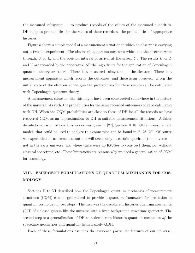
Figure 5 shows a simple model of a measurement situation in which an observer is carrying

out a two-slit experiment. The observer’s apparatus measures which slit the electron went

through, U or L, and the position interval of arrival at the screen Y . The results U or L

and Y are recorded by the apparatus. All the ingredients for the application of Copenhagen

quantum theory are there. There is a measured subsystem — the electron. There is a

measurement apparatus which records the outcomes, and there is an observer. Given the

initial state of the electron at the gun the probabilities for these results can be calculated

with Copenhagen quantum theory.

A measurement situation like this might have been constructed somewhere in the history

of the universe. As such, the probabilities for the same recorded outcomes could be calculated

with DH. When the CQM probabilities are close to those of DH for all the records we have

recovered CQM as an approximation to DH in suitable measurement situations. A fairly

detailed discussion of how this works was given in [27], Section II.10. Other measurement

models that could be used to analyze this connection can be found in [5, 28, 29]. Of course

we expect that measurement situations will occur only at certain epochs of the universe —

not in the early universe, not where there were no IGUSes to construct them, not without

classical spacetime, etc. These limitations are reasons why we need a generalization of CGM

for cosmology.

VIII. EMERGENT FORMULATIONS OF QUANTUM MECHANICS FOR COS-

MOLOGY

Sections II to VI described how the Copenhagen quantum mechanics of measurement

situations (CQM) can be generalized to provide a quantum framework for prediction in

quantum cosmology in two steps. The first was the decoherent histories quantum mechanics

(DH) of a closed system like the universe with a fixed background spacetime geometry. The

second step is a generalization of DH to a decoherent histories quantum mechanics of the

spacetime geometries and quantum fields namely GDH.

Each of these formulations assumes the existence particular features of our universe.

21

Copenhagen quantum mechanics assumes both a classical world containing laboratories with

measuring apparatus and observers that obey the laws of classical physics and a quantum

world of alternatives that are measured. Decoherent histories quantum mechanics assumed

a fixed background spacetime geometry. These features are examples of excess baggage11.

They are true physical facts but describe special situations in the the universe that occur

only at particular times and circumstances. We can say that they emerged at those particular

times and places in the evolution of our universe.

For example, in the early stages of the universe, spacetime geometry was fluctuating

quantum mechanically with no fixed value. As a consequence there was no fixed notion

of time and no fixed notion of spacelike or timelike. There then could be no notion of

quantum states defined on a foliating family of spacelike surfaces and, perforce, no notion

of the unitary evolution of states through such families of surfaces. There were no isolated

subsystems, and no notion of measurement of one by another. There were no observers

to exploit the regularities of the universe. The features of the universe assumed in the

formulation of the Copenhagen quantum mechanics and DH were not there in the early

universe.

Not much further on in the evolution of the universe classical spacetime emerged. With

it emerged the quasiclassical realm —– the wide range of time place and scale also on which

the deterministic laws of classical physics hold [31] . With it also emerged the notions of

time, states on spacelike surfaces and their unitary evolution by the Schrodinger equation

[8]. Eventually, galaxies, stars, planets, and biota emerged ∼ 1020 years later and with them

emerged the quasiclassical realm, and the observers, and measurements that are the subjects

of Copenhagen quantum theory. It is then, and only then, that Copenhagen quantum

mechanics is an appropriate approximation to the more general formulations12.

11 In many advances in physics some previously accepted general idea was found to be unnecessary and

dispensable. The idea was not truly a general feature of the world, but only perceived to be general

because of our special place in the universe and the limited range of our experience. It was excess baggage

which had to be jettisoned to reach a more a more general perspective [30]12 Thus only sufficiently late epochs of the universe will contain the observers necessary for Copenhagen

quantum mechanics. But also we cannot expect observers (including ourselves) very late in the universe’s

history. The cosmological constant causes the universe to expand and cool exponentially quickly. Stars

exhaust their thermonuclear fuel and die out. Black holes evaporate. The density of matter and the

temperature approach zero. Mechanisms of environmental decoherence fail [32]. The universe becomes

cold, dark and inhospitable to the formation and functioning of observers [33].

22

IX. CONCLUSION — ARE WE FINISHED GENERALIZING QUANTUM ME-

CHANICS?

The impacts of cosmology on quantum mechanics are at least these:

• Cosmology requires a quantum mechanics of a closed system in which measurements

and observers can be described but are not central the formulation of the theory.

• Cosmology requires a formulation of quantum mechanics general enough to deal with

quantum spacetime geometry, the big bang, and what emerged from it,

• Cosmology requires a formulation of quantum mechanics that can describe the emer-

gence of classical spacetime in the early early universe and along with it the quasiclassical

realm — the wide range of time, scale, and place that the classical laws of physics apply.

• Cosmology requires a formulation of quantum mechanics to which the Copenhagen

quantum mechanics is an approximation appropriate for measurement situations.

GDH potentially provides a generalization of CQM that can be applied to the prediction

of the outcomes of our cosmological observations from theories of the universe’s quantum

state Ψ and dynamics H. GDH is therefore a formulation that is adequate for quantum

cosmology. But it seems unlikely that it is the only possible adequate formulation. It is a

large and daring extrapolation to go from a quantum mechanics of laboratory situations to

a quantum mechanics of the whole universe. This is especially the case because the data

testing the extrapolation is very limited. Generalizations different from GDH are therefore

likely to be possible. Indeed, different routes to generalizations have already been suggested

[34–39]. A generalization of CQM does not just consist of a theory of dynamics (H) plus a

theory of the quantum state (Ψ). It also must specify the quantum framework for prediction

(Q). For the input theory in quantum cosmology we should write (H,Ψ, Q).

We hope to find generalizations Q that have less excess baggage than GDH such as a

principle of superposition for quantum states of the whole universe that can never be realized

experimentally. Perhaps even the notion of spacetime geometry is excess baggage. We hope

to find generalizations that are more deeply connected to ideas in contemporary fundamental

physics such as duality (e.g [40]). We hope to find generalizations that more deeply unify

the the theory of the quantum state Ψ and the theory of dynamics H. But above all we hope

to find generalizations that lead to definitive tests either in experiments in the laboratory or

by large scale observations. We are not yet finished understanding the impact of cosmology

23

on quantum mechanics.

Cosmology, quantum mechanics, and fundamental physics are inextricably but fruitfully

liked. The big bang is the place in the universe where the near Planck energy scales that

characterize much of today’s fundamental theory are reached. The observable consequences

of the big bang by which these theories might be tested are scattered over the large scales of

space and time observable today. We should not imagine that predicting these consequences

from (H,Ψ) is simply an a matter of calculating in a fixed quantum framework established

by low energy experiment. Rather, as we have seen in this paper, our understanding of

cosmology impacts our understanding of what is the quantum mechanics that applies to the

universe as a whole.

We end with a quotation that is the final paragraph of the first paper on decoherent

histories quantum mechanics [13]:

“We conclude that resolution of the problems of interpretation presented by quantum

mechanics is not to be accomplished by further intense scrutiny of the subject as it applies

to reproducible laboratory situations, but rather through an examination of the origin of the

universe and its subsequent history. Quantum mechanics is best and most fundamentally

understood in the context of quantum cosmology. The founders of quantum mechanics

were right in pointing out that something external to the framework of wave function and

Schrodinger equation is needed to interpret the theory. But it is not a postulated classical

world to which quantum mechanics does not apply. Rather it is the initial condition of the

universe that, together with the action function of the elementary particles and the throws

of quantum dice since the beginning, explains the origin of quasiclassical domain(s) within

quantum theory itself”.

Acknowledgments

The author thanks Murray Gell-Mann, Thomas Hertog, and Mark Srednicki for discus-

sions of the quantum mechanics of the universe over a long period of time. He thanks the

Santa Fe Institute for supporting many productive visits there. He thanks the organizers

of the conference 90 Years of Quantum Mechanics in Singapore which was the occasion of

a talk on which this work is partially based. The this work was supported in part by the

24

National Science Foundation under grant PHY15-04541 and PHY18-18018105 .

[1] M. Jammer, The Conceptual Development of Quantum Mechanics, (McGraw-Hill, New York,

1966).

[2] R. Penrose, Gravity’s Role in Quantum State Reduction, Gen. Rel. Grav. 28. 582 (1996);

A.J. Leggett, Testing the Limits of Quantum Mechanics: Motivation, State-of-Play, Prospects,

J. Phys. Cond. Matter 14, R415 (2002); P. Pearle and A. Valentini, Generalizations of Quan-

tum Mechanics, arXiv:quant-ph/0506115; S.Weinberg, Collapse of the State Vector, Phys.

Rev. A 85, 062116 (2012); S. Weinberg, Lectures on Quantum Mechanics, (CUP, Cambridge

2013) Chap 3; S. Weinberg, The Trouble with Quantum Mechanics, New York Review of

Books January 19, 2017; G. ‘t Hooft, The Cellular Automaton Interpretation of Quantum

Mechanics, Fundamental Theories of Physics, Vol. 185, Springer International Publishing,

2016; arXiv:1405.1548.

[3] S.Saunders, Decoherence and Ontology, in Many Worlds?, ed by S. Saunders, J. Barrett,

A.Kent and D. Wallace, (Oxford University Press, Oxford, 2010).

[4] L. D. Landau and E.M. Lifshitz, Quantum Mechanics (Eng. trans., Pergamon Press, 1958).

[5] J. von Neumann Mathematische Grundlagen der Quantenmechanik, J. Springer, Berlin (1932).

[English trans. Mathematical Foundations of Quantum Mechanics, Princeton University Press,

Princeton (1955)].

[6] A. Einstein, R. Tolman and B. Podolsky, Knowledge of the Past and Future in Quantum

Mechanics, Phys. Rev. 37, 780, 1931.

[7] J.B. Hartle, Quantum Pasts and the Utility of History, in The Proceedings of the Nobel

Symposium: Modern Studies of Basic Quantum Concepts and Phenomena, Gimo, Sweden,

June 13-17, 1997, Physica Scripta, T76, 67–77 (1998); arXiv:gr-qc/9712001.

[8] J.B. Hartle, The Spacetime Approach to Quantum Mechanics, Vistas in Astronomy , 37, 569,

(1993); arXiv: gr-qc/9304006.

[9] M. Gell-Mann and J.B Hartle, Quasiclassical Coarse Graining and Thermodynamic Entropy,

Phys. Rev. A, 76, 022104 (2007), arXiv:quant-ph/0609190.

[10] M. Gell-Mann and J.B. Hartle, Classical Equations for Quantum Systems, Phys. Rev. , D 47,

33453382, (1993); gr-qc/9210010.

25

[11] J.B. Hartle, S.W. Hawking, and T. Hertog, Classical Universes of the No-Boundary Quantum

State, Phys. Rev. D 77 123537 (2008), arXiv:0803:1663.

[12] R.B. Griffiths, Consistent Quantum Theory, Cambridge University Press, Cambridge, UK

(2002); R. Omnes, Interpretation of Quantum Mechanics, Princeton University Press, Prince-

ton (1994); M. Gell-Mann, The Quark and the Jaguar, W.H.. Freeman New York (1994);

M. Gell-Mann and J.B. Hartle, Quantum Mechanics in the Light of Quantum Cosmology,

in Complexity, Entropy, and the Physics of Information, ed. by W. Zurek, Addison Wesley,

Reading, MA (1990), P.C. Hohenberg, An introduction to consistent quantum theory, Rev.

Mod. Phys. , 82 2835-2844 (2010).

[13] M. Gell-Mann and J.B. Hartle, Quantum Mechanics in the Light of Quantum Cosmology,

in Complexity, Entropy, and the Physics of Information, ed. by W. Zurek, Addison Wesley,

Reading, MA (1990), arXiv:1803.04605.

[14] H. Everett III, Relative State formulation of Quantum Mechanics, Rev. Mod. Phys, 29, 454

(1957).

[15] J.B. Hartle, The Quantum Mechanics of Closed Systems, in Directions in General Relativity,

Volume 1, ed. by B.-L. Hu, M.P. Ryan, and C.V. Vishveshwara, Cambridge University Press,

Cambridge (1993), arXiv: gr-qc/9210006.

[16] R.P. Feynman and A.R. Hibbs, Quantum Mechanics and Path Integrals, (McGraw-Hill, New

York, 1964).

[17] E. Joos and H.D. Zeh, The emergence of classical properties through interaction with the

environment, Zeit. Phys. B, 59, 223 (1985).

[18] W. Zurek, Decoherence, einselection, and the quantum origins of the classical, Rev. Mod.

Phys. 75, 715 (2003).

[19] M. Gell-Mann and J.B, Hartle, Adaptive Coarse Graining, Environments, Strong Decoherence,

and Quasiclassical Realms, Phys. Rev. A 89, 052125 (2014); arXiv:1312.7454.

[20] J. B. Hartle and S. W. Hawking, The Wave Function of the Universe, Phys. Rev. D 28,

2960-2975 (1983).

[21] J.J. Halliwell, J.B. Hartle, and T. Hertog, What is the No-Boundary Wave Function of the

Universe; arXiv:1812 01760.

[22] J.B. Hartle, Spacetime Quantum Mechanics and the Quantum Mechanics of Spacetime in

Gravitation and Quantizations, Proceedings of the 1992 Les Houches Summer School, ed. by

26

B. Julia and J. Zinn-Justin, Les Houches Summer School Proceedings Vol. LVII, North Hol-

land, Amsterdam (1995); arXiv:gr-qc/9304006.

[23] J.B Hartle and T. Hertog, The Observer Strikes Back, in The Philosophy of Cosmology

ed. by K. Chamcham, J. Silk, J.D. Barrow, and S. Saunders, (Cambridge University Press,

Cambridge, 2017), p181-205, arXiv:1503.07205.

[24] S.W. Hawking and T. Hertog, Populating the Landscape: A Top Down Approach, Phys. Rev.

D 73, 123527 (2006), arXiv:hep-th/0602091

[25] J.B. Hartle and M. Srednicki, Are We Typical?, Phys. Rev. D, 75, 123523 (2007),

arXiv:0704:2630.

[26] M. Srednicki and J.B.Hartle, Science in a Very Large Universe, Phys. Rev. D, 81 123524

(2010), arXiv:0906.0042, a summary of this work with different emphases is in The Xerographic

Distribution: Scientific Reasoning in a Large Universe, arXiv:1004.3816.

[27] J.B. Hartle, The Quantum Mechanics of Cosmology, in Quantum Cosmology and Baby Uni-

verses: Proceedings of the 1989 Jerusalem Winter School for Theoretical Physics, ed. by

S. Coleman, J.B. Hartle, T. Piran, and S. Weinberg, World Scientific, Singapore (1991), pp.

65-157; arXiv:1805.12246. Section II.10

[28] F. London and E. Bauer, La theorie de l’observation en mecanique quantique, (Hermann,

Paris,1939).

[29] E. Wigner, The Problem of Measurement, Am. J. Phys. 31, 6, 1963.

[30] J.B. Hartle, Excess Baggage, in Elementary Particles and the Universe: Essays in Honor

of Murray Gell-Mann ed. by J. Schwarz, Cambridge University Press, Cambridge (1990);

arXiv:gr-qc/0508001.

[31] J.B. Hartle, The quasiclassical realms of this quantum universe, arXiv:0806.3776. A slightly

shorter version is published in Many Worlds? edited by S. Saunders, J. Barrett, A. Kent,

and D. Wallace (Oxford University Press, Oxford, 2010), the longer version was published in

Foundations of Physics, 41 982 (2011).

[32] J.B Hartle and T, Hertog, forthcoming.

[33] J.B. Hartle, Why Our Universe is Comprehensible; arXiv:1612.01952.

[34] J.B. Hartle, Linear Positivity and Virtual Probability, Phys. Rev. A, 70, 022104 (2004); arXiv;

quant-ph/0401108.

[35] J.B. Hartle, Generalizing Quantum Mechanics for Quantum Spacetime in The Quantum Struc-

27

ture of Space and Time: Proceedings of the 23rd Solvay Conference on Physics, ed. by

D. Gross, M Henneaux, and A. Sevrin, World Scientific, Singapore, 2007; arXiv:gr-qc/0602013.

[36] J.B. Hartle, Quantum Mechanics with Extended Probabilities, Phys. Rev. A 78, 012108 (2008),

arXiv:0801.0688.

[37] M. Gell-Mann and J.B. Hartle, Decoherent Histories Quantum Mechanics with One Real Fine-

Grained History, Phys. Rev. A 85, 062120 (2012); arXiv:1106.0767.

[38] J.B. Hartle, Decoherent Histories Quantum Mechanics Starting with Records of What Happens

arXiv:1608.04145.

[39] Steven B. Giddings, Universal Quantum Mechanics, Phys. Rev. D 78, 084004;

arXiv:0711.0757.

[40] T. Hertog and J.B. Hartle, Holographic No-Boundary Measure, JHEP, Number 5, 95 (2012);

arXiv:1111:6090.

28