
Martin Bojowald- Loop Quantum Cosmology
99
Living Rev. Re lativit y , 8, (2005), 11 http://www.livingreviews.org/lrr-2005-11 Loop Quantum Cosmology Martin Bojowald Max Planck Institute for Gravitational Physics (Albert Einstein Institute) Am M¨ uhlenberg 1, 14476 Potsdam, Germany and Institute for Gravitational Physics and Geometry The Pennsylvania State University University Park, PA 16802, U.S.A. email: [email protected] Accepted on 28 October 2005 Published on 8 December 2005 Living Reviews in Relativity Published by the Max Planck Institute for Gravitational Physics (Albert Einstein Institute) Am M¨ uhlenberg 1, 14424 Golm, Germany ISSN 1433-8351 Abstract Quantum gravity is expected to be necessary in order to understand situations where clas- sical general relativity breaks down. In particula r in cosmolo gy one has to deal with initial singularities, i.e., the fact that the back ward evolu tion of a classical space-time inevitably comes to an end after a finite amount of proper time. This presents a breakdown of the clas- sical picture and requires an extended theory for a meaningful description. Since small length scales and high curvatu res are inv olve d, quantum effects must play a role. Not only the singu- larit y itself but also the surroundin g space-time is then modified. One particula r realization is loop quantum cosmology, an application of loop quantum gravity to homogeneous systems, which removes classical singularities. Its implications can be studied at different levels. Main effects are introduced into effective classical equations which allow to avoid interpretational problems of quantum theory. They give rise to new kinds of early unive rse phenomeno logy with applications to inflation and cyclic models. To resolve classical singularities and to under- stand the structure of geometry around them, the quantum description is necessa ry . Classical evolution is then replaced by a difference equation for a wave function which allows to ex- tend space-time beyon d classical singularities . One main questio n is how these homogeneous scenarios are related to full loop quantum gravity, which can be dealt with at the level of dis- tribut ional symmetric states. Finally, the new structure of space-time arising in loop quan tum gravity and its application to cosmology sheds new light on more general issues such as time. c Max Planck Society and the authors. Further information on copyright is given at http://relativit y.livingreviews. org/About/copyri ght.html For permission to reproduce the article please contact [email protected].
Transcript of Martin Bojowald- Loop Quantum Cosmology

8/3/2019 Martin Bojowald- Loop Quantum Cosmology
http://slidepdf.com/reader/full/martin-bojowald-loop-quantum-cosmology 1/99
Living Rev. Relativity , 8, (2005), 11http://www.livingreviews.org/lrr-2005-11
Loop Quantum CosmologyMartin Bojowald
Max Planck Institute for Gravitational Physics(Albert Einstein Institute)
Am Muhlenberg 1, 14476 Potsdam, Germanyand
Institute for Gravitational Physics and GeometryThe Pennsylvania State UniversityUniversity Park, PA 16802, U.S.A.
email: [email protected]
Accepted on 28 October 2005Published on 8 December 2005
Living Reviews in Relativity
Published by theMax Planck Institute for Gravitational Physics
(Albert Einstein Institute)Am Muhlenberg 1, 14424 Golm, Germany
ISSN 1433-8351
Abstract
Quantum gravity is expected to be necessary in order to understand situations where clas-sical general relativity breaks down. In particular in cosmology one has to deal with initialsingularities, i.e., the fact that the backward evolution of a classical space-time inevitablycomes to an end after a finite amount of proper time. This presents a breakdown of the clas-sical picture and requires an extended theory for a meaningful description. Since small lengthscales and high curvatures are involved, quantum effects must play a role. Not only the singu-larity itself but also the surrounding space-time is then modified. One particular realizationis loop quantum cosmology, an application of loop quantum gravity to homogeneous systems,which removes classical singularities. Its implications can be studied at different levels. Maineffects are introduced into effective classical equations which allow to avoid interpretationalproblems of quantum theory. They give rise to new kinds of early universe phenomenologywith applications to inflation and cyclic models. To resolve classical singularities and to under-stand the structure of geometry around them, the quantum description is necessary. Classicalevolution is then replaced by a difference equation for a wave function which allows to ex-tend space-time beyond classical singularities. One main question is how these homogeneousscenarios are related to full loop quantum gravity, which can be dealt with at the level of dis-tributional symmetric states. Finally, the new structure of space-time arising in loop quantum
gravity and its application to cosmology sheds new light on more general issues such as time.
cMax Planck Society and the authors.Further information on copyright is given at
http://relativity.livingreviews.org/About/copyright.htmlFor permission to reproduce the article please contact [email protected].
8/3/2019 Martin Bojowald- Loop Quantum Cosmology
http://slidepdf.com/reader/full/martin-bojowald-loop-quantum-cosmology 2/99
How to cite this article
Owing to the fact that a Living Reviews article can evolve over time, we recommend to cite the
article as follows:
Martin Bojowald,“Loop Quantum Cosmology”,
Living Rev. Relativity , 8, (2005), 11. [Online Article]: cited [<date>],http://www.livingreviews.org/lrr-2005-11
The date given as <date> then uniquely identifies the version of the article you are referring to.
Article Revisions
Living Reviews supports two different ways to keep its articles up-to-date:
Fast-track revision A fast-track revision provides the author with the opportunity to add shortnotices of current research results, trends and developments, or important publications tothe article. A fast-track revision is refereed by the responsible subject editor. If an articlehas undergone a fast-track revision, a summary of changes will be listed here.
Major update A major update will include substantial changes and additions and is subject tofull external refereeing. It is published with a new publication number.
For detailed documentation of an article’s evolution, please refer always to the history document
of the article’s online version at http://www.livingreviews.org/lrr-2005-11.
8/3/2019 Martin Bojowald- Loop Quantum Cosmology
http://slidepdf.com/reader/full/martin-bojowald-loop-quantum-cosmology 3/99
Contents
1 Introduction 5
2 The Viewpoint of Loop Quantum Cosmology 6
3 Loop Quantum Gravity 83.1 Geometry . . . . . . . . . . . . . . . . . . . . . . . . . . . . . . . . . . . . . . . . . 83.2 Ashtekar variables . . . . . . . . . . . . . . . . . . . . . . . . . . . . . . . . . . . . 83.3 Representation . . . . . . . . . . . . . . . . . . . . . . . . . . . . . . . . . . . . . . 103.4 Function spaces . . . . . . . . . . . . . . . . . . . . . . . . . . . . . . . . . . . . . . 113.5 Composite operators . . . . . . . . . . . . . . . . . . . . . . . . . . . . . . . . . . . 123.6 Hamiltonian constraint . . . . . . . . . . . . . . . . . . . . . . . . . . . . . . . . . . 133.7 Open issues . . . . . . . . . . . . . . . . . . . . . . . . . . . . . . . . . . . . . . . . 14
4 Loop Cosmology 154.1 Isotropy . . . . . . . . . . . . . . . . . . . . . . . . . . . . . . . . . . . . . . . . . . 154.2 Isotropy: Connection variables . . . . . . . . . . . . . . . . . . . . . . . . . . . . . 164.3 Isotropy: Implications of a loop quantization . . . . . . . . . . . . . . . . . . . . . 174.4 Isotropy: Effective densities and equations . . . . . . . . . . . . . . . . . . . . . . . 184.5 Isotropy: Properties and intuitive meaning . . . . . . . . . . . . . . . . . . . . . . . 194.6 Isotropy: Applications . . . . . . . . . . . . . . . . . . . . . . . . . . . . . . . . . . 20
4.6.1 Collapsing phase . . . . . . . . . . . . . . . . . . . . . . . . . . . . . . . . . 204.6.2 Expansion . . . . . . . . . . . . . . . . . . . . . . . . . . . . . . . . . . . . . 214.6.3 Model building . . . . . . . . . . . . . . . . . . . . . . . . . . . . . . . . . . 244.6.4 Stability . . . . . . . . . . . . . . . . . . . . . . . . . . . . . . . . . . . . . . 24
4.7 Anisotropies . . . . . . . . . . . . . . . . . . . . . . . . . . . . . . . . . . . . . . . . 254.8 Anisotropy: Connection variables . . . . . . . . . . . . . . . . . . . . . . . . . . . . 264.9 Anisotropy: Applications . . . . . . . . . . . . . . . . . . . . . . . . . . . . . . . . 26
4.9.1 Isotropization . . . . . . . . . . . . . . . . . . . . . . . . . . . . . . . . . . . 264.9.2 Bianchi IX . . . . . . . . . . . . . . . . . . . . . . . . . . . . . . . . . . . . 274.9.3 Isotropic curvature suppression . . . . . . . . . . . . . . . . . . . . . . . . . 30
4.10 Anisotropy: Implications for inhomogeneities . . . . . . . . . . . . . . . . . . . . . 324.11 Inhomogeneities . . . . . . . . . . . . . . . . . . . . . . . . . . . . . . . . . . . . . . 324.12 Inhomogeneous matter with isotropic quantum geometry . . . . . . . . . . . . . . . 334.13 Inhomogeneity: Perturbations . . . . . . . . . . . . . . . . . . . . . . . . . . . . . . 344.14 Inhomogeneous models . . . . . . . . . . . . . . . . . . . . . . . . . . . . . . . . . . 344.15 Inhomogeneity: Results . . . . . . . . . . . . . . . . . . . . . . . . . . . . . . . . . 35
4.15.1 Matter gradient terms and small-a effects . . . . . . . . . . . . . . . . . . . 354.15.2 Matter gradient terms and large-a effects . . . . . . . . . . . . . . . . . . . 364.15.3 Non-inflationary structure formation . . . . . . . . . . . . . . . . . . . . . . 36
4.15.4 Stability . . . . . . . . . . . . . . . . . . . . . . . . . . . . . . . . . . . . . . 374.16 Summary . . . . . . . . . . . . . . . . . . . . . . . . . . . . . . . . . . . . . . . . . 37
5 Loop quantization of symmetric models 385.1 Symmetries and backgrounds . . . . . . . . . . . . . . . . . . . . . . . . . . . . . . 385.2 Isotropy . . . . . . . . . . . . . . . . . . . . . . . . . . . . . . . . . . . . . . . . . . 395.3 Isotropy: Matter Hamiltonian . . . . . . . . . . . . . . . . . . . . . . . . . . . . . . 405.4 Isotropy: Hamiltonian constraint . . . . . . . . . . . . . . . . . . . . . . . . . . . . 415.5 Semiclassical limit and correction terms . . . . . . . . . . . . . . . . . . . . . . . . 43
5.5.1 WKB approximation . . . . . . . . . . . . . . . . . . . . . . . . . . . . . . . 44
8/3/2019 Martin Bojowald- Loop Quantum Cosmology
http://slidepdf.com/reader/full/martin-bojowald-loop-quantum-cosmology 4/99
8/3/2019 Martin Bojowald- Loop Quantum Cosmology
http://slidepdf.com/reader/full/martin-bojowald-loop-quantum-cosmology 5/99
Loop Quantum Cosmology 5
1 Introduction
Die Grenzen meiner Sprache bedeuten die Grenzen meiner Welt.
(The limits of my language mean the limits of my world.) Ludwig Wittgenstein
Tractatus logico-philosophicus
While general relativity is very successful in describing the gravitational interaction and thestructure of space and time on large scales [205], quantum gravity is needed for the small-scalebehavior. This is usually relevant when curvature, or in physical terms energy densities and tidalforces, becomes large. In cosmology this is the case close to the Big Bang, and also in the interiorof black holes. We are thus able to learn about gravity on small scales by looking at the earlyhistory of the universe.
Starting with general relativity on large scales and evolving backward in time, the universebecomes smaller and smaller and quantum effects eventually become important. That the classicaltheory by itself cannot be sufficient to describe the history in a well-defined way is illustrated by
singularity theorems [123] which also apply in this case: After a finite time of backward evolutionthe classical universe will collapse into a single point and energy densities diverge. At this point,the theory breaks down and cannot be used to determine what is happening there. Quantumgravity, with its different dynamics on small scales, is expected to solve this problem.
The quantum description does not only present a modified dynamical behavior on small scalesbut also a new conceptual setting. Rather than dealing with a classical space-time manifold, wenow have evolution equations for the wave function of a universe. This opens a vast numberof problems on various levels from mathematical physics to cosmological observations, and evenphilosophy. This review is intended to give an overview and summary of the current status of thoseproblems, in particular in the new framework of loop quantum cosmology.
Living Reviews in Relativity http://www.livingreviews.org/lrr-2005-11
8/3/2019 Martin Bojowald- Loop Quantum Cosmology
http://slidepdf.com/reader/full/martin-bojowald-loop-quantum-cosmology 6/99
6 Martin Bojowald
2 The Viewpoint of Loop Quantum Cosmology
Loop quantum cosmology is based on quantum Riemannian geometry, or loop quantum gravity[172, 22, 195, 174], which is an attempt at a non-perturbative and background independent quan-tization of general relativity. This means that no assumptions of small fields or the presence of aclassical background metric are made, both of which is expected to be essential close to classicalsingularities where the gravitational field would diverge and space degenerates. In contrast to otherapproaches to quantum cosmology there is a direct link between cosmological models and the fulltheory [38, 66], as we will describe later in Section 6. With cosmological applications we are thusable to test several possible constructions and draw conclusions for open issues in the full theory.At the same time, of course, we can learn about physical effects which have to be expected fromproperties of the quantization and can potentially lead to observable predictions. Since the fulltheory is not completed yet, however, an important issue in this context is the robustness of thoseapplications to choices in the full theory and quantization ambiguities.
The full theory itself is, understandably, extremely complex and thus requires approximationschemes for direct applications. Loop quantum cosmology is based on symmetry reduction, in
the simplest case to isotropic geometries [46]. This poses the mathematical problem as to how thequantum representation of a model and its composite operators can be derived from that of the fulltheory, and in which sense this can be regarded as an approximation with suitable correction terms.Research in this direction currently proceeds by studying symmetric models with less symmetriesand the relations between them. This allows to see what role anisotropies and inhomogeneitiesplay in the full theory.
While this work is still in progress, one can obtain full quantizations of models by using basicfeatures as they can already be derived from the full theory together with constructions of morecomplicated operators in a way analogous to what one does in the full theory (see Section 5). Forthose complicated operators, the prime example being the Hamiltonian constraint which dictatesthe dynamics of the theory, the link between model and the full theory is not always clear-cut.Nevertheless, one can try different versions in the model in explicit ways and see what implications
this has, so again the robustness issue arises. This has already been applied to issues such asthe semiclassical limit and general properties of quantum dynamics. Thus, general ideas whichare required for this new, background independent quantization scheme, can be tried in a rathersimple context in explicit ways to see how those constructions work in practice.
At the same time, there are possible phenomenological consequences in the physical systemsbeing studied, which is the subject of Section 4. In fact it turned out, rather surprisingly, thatalready very basic effects such as the discreteness of quantum geometry and other features brieflyreviewed in Section 3, for which a reliable derivation from the full theory is available, have veryspecific implications in early universe cosmology. While quantitative aspects depend on quantiza-tion ambiguities, there is a rich source of qualitative effects which work together in a well-definedand viable picture of the early universe. In such a way, as illustrated later, a partial view of thefull theory and its properties emerges also from a physical, not just mathematical perspective.
With this wide range of problems being investigated we can keep our eyes open to inputfrom all sides. There are mathematical consistency conditions in the full theory, some of whichare identically satisfied in the simplest models (such as the isotropic model which has only oneHamiltonian constraint and thus a trivial constraint algebra). They are being studied in different,more complicated models and also in the full theory directly. Since the conditions are not easyto satisfy, they put stringent bounds on possible ambiguities. From physical applications, on theother hand, we obtain conceptual and phenomenological constraints which can be complementaryto those obtained from consistency checks. All this contributes to a test and better understandingof the background independent framework and its implications.
Other reviews of loop quantum cosmology at different levels can be found in [ 56, 55, 199, 50,
Living Reviews in Relativity http://www.livingreviews.org/lrr-2005-11
8/3/2019 Martin Bojowald- Loop Quantum Cosmology
http://slidepdf.com/reader/full/martin-bojowald-loop-quantum-cosmology 7/99
Loop Quantum Cosmology 7
69, 51, 96]. For complementary applications of loop quantum gravity to cosmology see [140, 141,2, 114, 152, 1].
Living Reviews in Relativity http://www.livingreviews.org/lrr-2005-11
8/3/2019 Martin Bojowald- Loop Quantum Cosmology
http://slidepdf.com/reader/full/martin-bojowald-loop-quantum-cosmology 8/99
8 Martin Bojowald
3 Loop Quantum Gravity
Since many reviews of full loop quantum gravity [172, 195, 22, 174, 161] as well as shorter accounts[9, 10, 173, 190, 167, 198] are already available, we describe here only those properties which will
be essential later on. Nevertheless, this review is mostly self-contained; our notation is closest tothat in [22]. A recent bibliography can be found in [93].
3.1 Geometry
General relativity in its canonical formulation [6] describes the geometry of space-time in termsof fields on spatial slices. Geometry on such a spatial slice Σ is encoded in the spatial metric qab,which presents the configuration variables. Canonical momenta are given in terms of extrinsiccurvature K ab which is the derivative of the spatial metric under changing the spatial slice. Thosefields are not arbitrary since they are obtained from a solution of Einstein’s equations by choosinga time coordinate defining the spatial slices, and space-time geometry is generally covariant. In thecanonical formalism this is expressed by the presence of constraints on the fields, the diffeomorphism
constraint and the Hamiltonian constraint. The diffeomorphism constraint generates deformationsof a spatial slice or coordinate changes, and when it is satisfied spatial geometry does not dependon which coordinates we choose on space. General covariance of space-time geometry also forthe time coordinate is then completed by imposing the Hamiltonian constraint. This constraint,furthermore, is important for the dynamics of the theory: Since there is no absolute time, there isno Hamiltonian generating evolution, but only the Hamiltonian constraint. When it is satisfied, itencodes correlations between the physical fields of gravity and matter such that evolution in thisframework is relational. The reproduction of a space-time metric in a coordinate dependent waythen requires to choose a gauge and to compute the transformation in gauge parameters (includingthe coordinates) generated by the constraints.
It is often useful to describe spatial geometry not by the spatial metric but by a triad eai whichdefines three vector fields which are orthogonal to each other and normalized in each point. Thisyields all information about spatial geometry, and indeed the inverse metric is obtained from the
triad by qab = eai ebi where we sum over the index i counting the triad vector fields. There aredifferences, however, between metric and triad formulations. First, the set of triad vectors can berotated without changing the metric, which implies an additional gauge freedom with group SO(3)acting on the index i. Invariance of the theory under those rotations is then guaranteed by a Gaussconstraint in addition to the diffeomorphism and Hamiltonian constraints.
The second difference will turn out to be more important later on: We can not only rotatethe triad vectors but also reflect them, i.e., change the orientation of the triad given by sgn det eai .This does not change the metric either, and so could be included in the gauge group as O(3).However, reflections are not connected to the unit element of O(3) and thus are not generated bya constraint. It then has to be seen whether or not the theory allows to impose invariance underreflections, i.e., if its solutions are reflection symmetric. This is not usually an issue in the classicaltheory since positive and negative orientations on the space of triads are separated by degenerate
configurations where the determinant of the metric vanishes. Points on the boundary are usuallysingularities where the classical evolution breaks down such that we will never connect betweenboth sides. However, since there are expectations that quantum gravity may resolve classicalsingularities, which indeed are confirmed in loop quantum cosmology, we will have to keep thisissue in mind and not restrict to only one orientation from the outset.
3.2 Ashtekar variables
To quantize a constrained canonical theory one can use Dirac’s prescription [ 105] and first representthe classical Poisson algebra of a suitable complete set of basic variables on phase space as an
Living Reviews in Relativity http://www.livingreviews.org/lrr-2005-11
8/3/2019 Martin Bojowald- Loop Quantum Cosmology
http://slidepdf.com/reader/full/martin-bojowald-loop-quantum-cosmology 9/99
Loop Quantum Cosmology 9
operator algebra on a Hilbert space, called kinematical. This ignores the constraints, which canbe written as operators on the same Hilbert space. At the quantum level the constraints arethen solved by determining their kernel, to be equipped with an inner product so as to define thephysical Hilbert space. If zero is in the discrete part of the spectrum of a constraint, as e.g., for theGauss constraint when the structure group is compact, the kernel is a subspace of the kinematicalHilbert space to which the kinematical inner product can be restricted. If, on the other hand, zerolies in the continuous part of the spectrum, there are no normalizable eigenstates and one has toconstruct a new physical Hilbert space from distributions. This is the case for the diffeomorphismand Hamiltonian constraints.
To perform the first step we need a Hilbert space of functionals ψ[q] of spatial metrics. Un-fortunately, the space of metrics, or alternatively extrinsic curvature tensors, is mathematicallypoorly understood and not much is known about suitable inner products. At this point, a newset of variables introduced by Ashtekar [7, 8, 30] becomes essential. This is a triad formulation,but uses the triad in a densitized form (i.e., it is multiplied with an additional factor of a Jaco-bian under coordinate transformations). The densitized triad E ai is then related to the triad by
E ai = det ebj−1
eai but has the same properties concerning gauge rotations and its orientation (note
the absolute value which is often omitted). The densitized triad is conjugate to extrinsic curvaturecoefficients K ia := K abebi :
K ia(x), E bj (y) = 8πGδbaδijδ(x, y) (1)
with the gravitational constant G. Extrinsic curvature is then replaced by the Ashtekar connection
Aia = Γia + γK ia (2)
with a positive value for γ , the Barbero–Immirzi parameter [30, 133]. Classically, this numbercan be changed by a canonical transformation of the fields, but it will play a more important andfundamental role upon quantization. The Ashtekar connection is defined in such a way that it isconjugate to the triad,
Aia(x), E bj (y)
= 8πγGδbaδijδ(x, y) (3)
and obtains its transformation properties as a connection from the spin connection
Γia = −ijkebj(∂ [aeke] + 12 eckela∂ [celb]). (4)
Spatial geometry is then obtained directly from the densitized triad, which is related to thespatial metric by
E ai E bi = qab det q.
There is more freedom in a triad since it can be rotated without changing the metric. The theoryis independent of such rotations provided the Gauss constraint
G[Λ] =1
8πγG Σ d3x ΛiDaE a
i=
1
8πγG Σ d3x Λi(∂ aE a
i+ ijkAj
aE a
k)≈
0 (5)
is satisfied. Independence from any spatial coordinate system or background is implemented bythe diffeomorphism constraint (modulo Gauss constraint)
D[N a] =1
8πγG
Σ
d3x N aF iabE bi ≈ 0, (6)
with the curvature F iab of the Ashtekar connection. In this setting, one can then discuss spatialgeometry and its quantization.
Living Reviews in Relativity http://www.livingreviews.org/lrr-2005-11
8/3/2019 Martin Bojowald- Loop Quantum Cosmology
http://slidepdf.com/reader/full/martin-bojowald-loop-quantum-cosmology 10/99
10 Martin Bojowald
Space-time geometry, however, is more complicated to deduce since it requires a good knowledgeof the dynamics. In a canonical setting, dynamics is implemented by the Hamiltonian constraint
H [N ] =
1
16πγG Σ d3
x N |det E |−1/2 ijkF
i
abE a
j E b
k − 2(1 + γ 2
)K i
[aK
j
b]E a
i E b
j ≈ 0, (7)
where extrinsic curvature components have to be understood as functions of the Ashtekar connec-tion and the densitized triad through the spin connection.
3.3 Representation
The key new aspect is now that we can choose the space of Ashtekar connections as our configura-tion space whose structure is much better understood than that of a space of metrics. Moreover,the formulation lends itself easily to a background independent quantization. To see this we needto remember that quantizing field theories requires one to smear fields, i.e., to integrate them overregions in order to obtain a well-defined algebra without δ-functions as in Equation (3). Usuallythis is done by integrating both configuration and momentum variables over three-dimensionalregions, which requires an integration measure. This is no problem in ordinary field theories,which are formulated on a background such as Minkowski or a curved space. However, doing thishere for gravity in terms of Ashtekar variables would immediately spoil any possible backgroundindependence since a background would already occur at this very basic step.
There is now a different smearing available that does not require a background metric. Insteadof using three-dimensional regions we integrate the connection along one-dimensional curves e andexponentiate in a path-ordered manner, resulting in holonomies
he(A) = P exp
e
τ iAiaea dt (8)
with tangent vector ea to the curve e and τ j = − 12
iσj in terms of Pauli matrices. The path
ordered exponentiation needs to be done in order to obtain a covariant object from the non-Abelian connection. The prevalence of holonomies or, in their most simple gauge invariant formas Wilson loops trhe(A) for closed e, is the origin of loop quantum gravity and its name [175].Similarly, densitized vector fields can naturally be integrated over 2-dimensional surfaces, resultingin fluxes
F S(E ) =
S
τ iE ai na d2y (9)
with the co-normal na to the surface.The Poisson algebra of holonomies and fluxes is now well-defined and one can look for repre-
sentations on a Hilbert space. We also require diffeomorphism invariance, i.e., there must be aunitary action of the diffeomorphism group on the representation by moving edges and surfacesin space. This is required since the diffeomorphism constraint has to be imposed later. Under
this condition, there is even a unique representation that defines the kinematical Hilbert space[179, 180, 164, 183, 113, 146].We can construct the Hilbert space in the representation where states are functionals of con-
nections. This can easily be done by using holonomies as “creation operators” starting with a“ground state” which does not depend on connections at all. Multiplying with holonomies thengenerates states that do depend on connections, but only along the edges used in the process.These edges can be collected in a graph appearing as a label of the state. An independent setof states is given by spin network states [178] associated with graphs whose edges are labeled byirreducible representations of the gauge group SU(2), in which to evaluate the edge holonomies,and whose vertices are labeled by matrices specifying how holonomies leaving or entering the vertex
Living Reviews in Relativity http://www.livingreviews.org/lrr-2005-11
8/3/2019 Martin Bojowald- Loop Quantum Cosmology
http://slidepdf.com/reader/full/martin-bojowald-loop-quantum-cosmology 11/99
Loop Quantum Cosmology 11
are multiplied together. The inner product on this state space is such that these states, with anappropriate definition of independent contraction matrices in vertices, are orthonormal.
Spatial geometry can be obtained from fluxes representing the densitized triad. Since these arenow momenta, they are represented by derivative operators with respect to values of connections onthe flux surface. States as constructed above depend on the connection only along edges of graphssuch that the flux operator is non-zero only if there are intersection points between its surface andthe graph in the state it acts on [145]. Moreover, the contribution from each intersection pointcan be seen to be analogous to an angular momentum operator in quantum mechanics which hasa discrete spectrum [20]. Thus, when acting on a given state we obtain a finite sum of discretecontributions and thus a discrete spectrum of flux operators. The spectrum depends on the value of the Barbero–Immirzi parameter, which can accordingly be fixed using implications of the spectrumsuch as black hole entropy, which gives a value of the order of but smaller than one [11, 12, 108, 155].Moreover, since angular momentum operators do not commute, flux operators do not commute ingeneral [17]. There is thus no triad representation, which is another reason why using a metricformulation and trying to build its quantization with functionals on a metric space is difficult.
There are important basic properties of this representation, which we will use later on. First,
as already noted, flux operators have discrete spectra and, secondly, holonomies of connections arewell-defined operators. It is, however, not possible to obtain operators for connection components ortheir integrations directly but only in the exponentiated form. These are direct consequences of thebackground independent quantization and translate to particular properties of more complicatedoperators.
3.4 Function spaces
A connection 1-form Aia can be reconstructed uniquely if all its holonomies are known [118]. It
is thus sufficient to parameterize the configuration space by matrix elements of he for all edgesin space. This defines an algebra of functions on the infinite dimensional space of connectionsA, which are multiplied as C-valued functions. Moreover, there is a duality operation by complexconjugation, and if the structure group G is compact a supremum norm exists since matrix elementsof holonomies are then bounded. Thus, matrix elements form an Abelian C ∗-algebra with unit asa subalgebra of all continuous functions on A.
Any Abelian C ∗-algebra with unit can be represented as the algebra of all continuous func-tions on a compact space A. The intuitive idea is that the original space A, which has manymore continuous functions, is enlarged by adding new points to it. This increases the number of continuity conditions and thus shrinks the set of continuous functions. This is done until onlymatrix elements of holonomies survive when continuity is imposed, and it follows from generalresults that the enlarged space must be compact for an Abelian unital C ∗-algebra. We thus obtaina compactification A, the space of generalized connections [23], which densely contains the spaceA.
There is a natural diffeomorphism invariant measure dµAL on A, the Ashtekar–Lewandowskimeasure [19], which defines the Hilbert space
H= L2(
A, dµAL) of square integrable functions
on the space of generalized connections. A dense subset Cyl of functions is given by cylindricalfunctions f (he1 , . . . , hen), which depend on the connection through a finite but arbitrary numberof holonomies. They are associated with graphs g formed by the edges e1, . . . , en. For functionscylindrical with respect to two identical graphs the inner product can be written as
f |g =
A
dµAL(A)f (A)∗g(A) =
SU(2)n
ni=1
dµH(hi)f (h1, . . . , hn)∗g(h1, . . . , hn) (10)
with the Haar measure dµH on G. The importance of generalized connections can be seen fromthe fact that the space A of smooth connections is a subset of measure zero in A [154].
Living Reviews in Relativity http://www.livingreviews.org/lrr-2005-11
8/3/2019 Martin Bojowald- Loop Quantum Cosmology
http://slidepdf.com/reader/full/martin-bojowald-loop-quantum-cosmology 12/99
12 Martin Bojowald
With the dense subset Cyl of H we obtain the Gel’fand triple
Cyl ⊂ H ⊂ Cyl∗ (11)
with the dual Cyl∗ of linear functionals from Cyl to the set of complex numbers. Elements of Cyl∗ are distributions, and there is no inner product on the full space. However, one can defineinner products on certain subspaces defined by the physical context. Often, those subspaces appearwhen constraints with continuous spectra are solved following the Dirac procedure. Other examplesinclude the definition of semiclassical or, as we will use in Section 6, symmetric states.
3.5 Composite operators
From the basic operators we can construct more complicated ones which, with growing degree of complexity, will be more and more ambiguous for instance from factor ordering choices. Quitesimple expressions exist for the area and volume operator [177, 20, 21], which are constructedsolely from fluxes. Thus, they are less ambiguous since no factor ordering issues with holonomies
arise. This is true because the area of a surface and volume of a region can be written classicallyas functionals of the densitized triad alone, AS = S E ai naE binbd2y and V R =
R |det E ai |d3x.
At the quantum level, this implies that, just as fluxes, also area and volume have discrete spectrashowing that spatial quantum geometry is discrete. (For discrete approaches to quantum gravityin general see [150].) All area eigenvalues are known explicitly, but this is not possible even inprinciple for the volume operator. Nevertheless, some closed formulas and numerical techniquesexist [149, 103, 102, 83].
The length of a curve, on the other hand, requires the co-triad which is an inverse of thedensitized triad and is more problematic. Since fluxes have discrete spectra containing zero, theydo not have densely defined inverse operators. As we will describe below, it is possible to quantizethose expressions but requires one to use holonomies. Thus, here we encounter more ambiguitiesfrom factor ordering. Still, one can show that also length operators have discrete spectra [192].
Inverse densitized triad components also arise when we try to quantize matter Hamiltonians
such as
H φ =
d3x
1
2
p2φ + E ai E bi ∂ aφ∂ bφ det E cj
+ det E cj
V (φ)
(12)
for a scalar field φ with momentum pφ and potential V (φ) (not to be confused with volume). Theinverse determinant again cannot be quantized directly by using, e.g., an inverse of the volumeoperator which does not exist. This seems, at first, to be a severe problem not unlike the situationin quantum field theory on a background where matter Hamiltonians are divergent. Yet, it turnsout that quantum geometry allows one to quantize these expressions in a well-defined manner [ 193].
To do this, we notice that the Poisson bracket of the volume with connection components,
Aia, |det E |d
3
x = 2πγGijk
abcE bjE ck |det E | , (13)
amounts to an inverse of densitized triad components and does allow a well-defined quantization:we can express the connection component through holonomies, use the volume operator and turnthe Poisson bracket into a commutator. Since all operators involved have a dense intersection of their domains of definition, the resulting operator is densely defined and amounts to a quantizationof inverse powers of the densitized triad.
This also shows that connection components or holonomies are required in this process, and
thus ambiguities can arise even if initially one starts with an expression such as
|det E |−1, which
Living Reviews in Relativity http://www.livingreviews.org/lrr-2005-11
8/3/2019 Martin Bojowald- Loop Quantum Cosmology
http://slidepdf.com/reader/full/martin-bojowald-loop-quantum-cosmology 13/99
Loop Quantum Cosmology 13
only depends on the triad. There are also many different ways to rewrite expressions as above,which all are equivalent classically but result in different quantizations. In classical regimes thiswould not be relevant, but can have sizeable effects at small scales. In fact, this particular aspect,which as a general mechanism is a direct consequence of the background independent quantizationwith its discrete fluxes, implies characteristic modifications of the classical expressions on smallscales. We will discuss this and more detailed examples in the cosmological context in Section 4.
3.6 Hamiltonian constraint
Similarly to matter Hamiltonians one can also quantize the Hamiltonian constraint in a well-definedmanner [194]. Again, this requires to rewrite triad components and to make other regularizationchoices. Thus, there is not just one quantization but a class of different possibilities.
It is more direct to quantize the first part of the constraint containing only the Ashtekarcurvature. (This part agrees with the constraint in Euclidean signature and Barbero–Immirziparameter γ = 1, and so is sometimes called Euclidean part of the constraint.) Triad components
and their inverse determinant are again expressed as a Poisson bracket using the identity ( 13), andcurvature components are obtained through a holonomy around a small loop α of coordinate size∆ and with tangent vectors sa1 and sa2 at its base point [176]:
sa1sb2F iabτ i = ∆−1(hα − 1) + O(∆). (14)
Putting this together, an expression for the Euclidean part H E[N ] can then be constructed in theschematic form
H E[N ] ∝v
N (v)IJK tr
hαIJ hsKh−1sK
, V + O(∆), (15)
where one sums over all vertices of a triangulation of space whose tetrahedra are used to define
closed curves αIJ and transversal edges sK .An important property of this construction is that coordinate functions such as ∆ disappear
from the leading term, such that the coordinate size of the discretization is irrelevant. Nevertheless,there are several choices to be made, such as how a discretization is chosen in relation to a graphthe constructed operator is supposed to act on, which in later steps will have to be constrained bystudying properties of the quantization. Of particular interest is the holonomy hα since it createsnew edges to a graph, or at least new spin on existing ones. Its precise behavior is expected tohave a strong influence on the resulting dynamics [189]. In addition, there are factor orderingchoices, i.e., whether triad components appear to the right or left of curvature components. Itturns out that the expression above leads to a well-defined operator only in the first case, which inparticular requires an operator non-symmetric in the kinematical inner product. Nevertheless, onecan always take that operator and add its adjoint (which in this full setting does not simply amountto reversing the order of the curvature and triad expressions) to obtain a symmetric version, suchthat the choice still exists. Another choice is the representation chosen to take the trace, whichfor the construction is not required to be the fundamental one [ 116].
The second part of the constraint is more complicated since one has to use the function Γ(E ) inK ia. As also developed in [194], extrinsic curvature can be obtained through the already constructedEuclidean part via K ∼ H E, V . The result, however, is rather complicated, and in models oneoften uses a more direct way exploiting the fact that Γ has a more special form. In this way,additional commutators in the general construction can be avoided, which usually does not havestrong effects. Sometimes, however, these additional commutators can be relevant, which canalways be decided by a direct comparison of different constructions (see, e.g., [125]).
Living Reviews in Relativity http://www.livingreviews.org/lrr-2005-11
8/3/2019 Martin Bojowald- Loop Quantum Cosmology
http://slidepdf.com/reader/full/martin-bojowald-loop-quantum-cosmology 14/99
14 Martin Bojowald
3.7 Open issues
For an anomaly-free quantization the constraint operators have to satisfy an algebra mimickingthe classical one. There are arguments that this is the case for the quantization as described above
when each loop α contains exactly one vertex of a given graph [191], but the issue is still open.Moreover, the operators are quite complicated and it is not easy to see if they have the correctexpectation values in appropriately defined semiclassical states.
Even if one regards the quantization and semiclassical issues as satisfactory, one has to faceseveral hurdles in evaluating the theory. There are interpretational issues of the wave functionobtained as a solution to the constraints, and also the problem of time or observables emerges[143]. There is a wild mixture of conceptual and technical problems at different levels, not at leastbecause the operators are quite complicated. For instance, as seen in the rewriting procedure above,the volume operator plays an important role even if one is not necessarily interested in the volumeof regions. Since this operator is complicated, without an explicitly known spectrum, it translatesto complicated matrix elements of the constraints and matter Hamiltonians. Loop quantum gravityshould thus be considered as a framework rather than a uniquely defined theory, which however
has important rigid aspects. This includes the basic representation of the holonomy-flux algebraand its general consequences.All this should not come as a surprise since even classical gravity, at this level of generality, is
complicated enough. Most solutions and results in general relativity are obtained with approxima-tions or assumptions, one of the most widely used being symmetry reduction. In fact, this allowsaccess to the most interesting gravitational phenomena such as cosmological expansion, black holesand gravitational waves. Similarly, symmetry reduction is expected to simplify many problems of full quantum gravity by resulting in simpler operators and by isolating conceptual problems suchthat not all of them need to be considered at once.
Living Reviews in Relativity http://www.livingreviews.org/lrr-2005-11
8/3/2019 Martin Bojowald- Loop Quantum Cosmology
http://slidepdf.com/reader/full/martin-bojowald-loop-quantum-cosmology 15/99
Loop Quantum Cosmology 15
4 Loop Cosmology
Je abstrakter die Wahrheit ist, die du lehren willst, um so mehr mußt du noch die Sinnezu ihr verf¨ uhren.
(The more abstract the truth you want to teach is, the more you have to seduce to it the senses.)
Friedrich Nietzsche
Beyond Good and Evil
The gravitational field equations, for instance in the case of cosmology where one can as-sume homogeneity and isotropy, involve components of curvature as well as the inverse metric.(Computational methods to derive information from these equations are described in [5].) Sincesingularities occur, these components will become large in certain regimes, but the equations havebeen tested only in small curvature regimes. On small length scales such as close to the Big Bang,modifications to the classical equations are not ruled out by observations and can be expectedfrom candidates of quantum gravity. Quantum cosmology describes the evolution of a universe bya constraint equation for a wave function, but some effects can be included already at the levelof effective classical equations. In loop quantum gravity, the main modification happens throughinverse metric components which, e.g., appear in the kinematic term of matter Hamiltonians. Thisone modification is mainly responsible for all the diverse effects of loop cosmology.
4.1 Isotropy
Isotropy reduces the phase space of general relativity to be 2-dimensional since, up to SU(2)-gaugefreedom, there is only one independent component in an isotropic connection and triad, respectively,which is not already determined by the symmetry. This is analogous to metric variables, wherethe scale factor a is the only free component in the spatial part of an isotropic metric
ds2 = −N (t)2 dt2 + a(t)2((1 − kr2)−1 dr2 + r2 dΩ2). (16)
The lapse function N (t) does not play a dynamical role and correspondingly does not appear inthe Friedmann equation
a
a
2
+k
a2=
8πG
3a−3H matter(a) (17)
with the matter Hamiltonian H matter and the gravitational constant G, and the parameter k takingthe discrete values zero or ±1 depending on the symmetry group or intrinsic spatial curvature.
Indeed, N (t) can simply be absorbed into the time coordinate by defining proper time τ throughdτ = N (t)dt. This is not possible for the scale factor since it depends on time but multiplies spacedifferentials in the line element. The scale factor can only be rescaled by an arbitrary constant,
which can be normalized at least in the closed model where k = 1.One can understand these different roles of metric components also from a Hamiltonian analysis
of the Einstein–Hilbert action
S EH =1
16πG
dt d3xR[g]
specialized to isotropic metrics (16) whose Ricci scalar is
R = 6
a
N 2a+
a2
N 2a2+
k
a2− a
a
N
N 3
.
Living Reviews in Relativity http://www.livingreviews.org/lrr-2005-11
8/3/2019 Martin Bojowald- Loop Quantum Cosmology
http://slidepdf.com/reader/full/martin-bojowald-loop-quantum-cosmology 16/99
16 Martin Bojowald
The action then becomes
S =V 0
16πG dt Na3R =
3V 08πG
dt N
−aa2
N 2+ ka
(with the spatial coordinate volume V 0 =
Σ
d3x) after integrating by parts, from which one derivesthe momenta
pa =∂L
∂ a= − 3V 0
4πG
aa
N , pN =
∂L
∂ N = 0
illustrating the different roles of a and N . Since pN must vanish, N is not a degree of freedom buta Lagrange multiplier. It appears in the canonical action S = (16πG)−1
dt(apa − N H )) only as
a factor of
H = −2πG
3
p2a
V 0a− 3
8πGV 0ak
such that variation with respect to N forces H , the Hamiltonian constraint, to be zero. In thepresence of matter, H also contains the matter Hamiltonian, and its vanishing is equivalent to theFriedmann equation.
4.2 Isotropy: Connection variables
Isotropic connections and triads, as discussed in Appendix B.2, are analogously described by singlecomponents c and ˜ p, respectively, related to the scale factor by
|˜ p| = a2 =a2
4(18)
for the densitized triad component ˜ p and
c = Γ + γ ˙a =
1
2 (k + γ a) (19)
for the connection component c. Both components are canonically conjugate:
c, ˜ p =8πγG
3V 0. (20)
It is convenient to absorb factors of V 0 into the basic variables, which is also suggested by theintegrations in holonomies and fluxes on which background independent quantizations are built[15]. We thus define
p = V 2/3
0 ˜ p, c= V 1/3
0 c (21)
together with Γ = V 1/3
0 Γ. The symplectic structure is then independent of V 0 and so are integrated
densities such as total Hamiltonians. For the Hamiltonian constraint in isotropic Ashtekar variableswe have
H = − 3
8πG(γ −2(c − Γ)2 + Γ2)
| p| + H matter( p) = 0, (22)
which is exactly the Friedmann equation. (In most earlier papers on loop quantum cosmology somefactors in the basic variables and classical equations are incorrect due, in part, to the existence of different and often confusing notations in the loop quantum gravity literature.1)
1The author is grateful to Ghanashyam Date and Golam Hossain for discussions and correspondence on thisissue.
Living Reviews in Relativity http://www.livingreviews.org/lrr-2005-11
8/3/2019 Martin Bojowald- Loop Quantum Cosmology
http://slidepdf.com/reader/full/martin-bojowald-loop-quantum-cosmology 17/99
Loop Quantum Cosmology 17
The part of phase space where we have p = 0 and thus a = 0 plays a special role since this iswhere isotropic classical singularities are located. On this subset the evolution equation (17) withstandard matter choices is singular in the sense that H matter, e.g.,
H φ(a,φ,pφ) = 12| p|−3/2 p2
φ + | p|3/2V (φ) (23)
for a scalar φ with momentum pφ and potential V (φ), diverges and the differential equation doesnot pose a well-defined initial value problem there. Thus, once such a point is reached the furtherevolution is no longer determined by the theory. Since, according to singularity theorems [123, 80],any classical trajectory must intersect the subset a = 0 for the matter we need in our universe, theclassical theory is incomplete.
This situation, certainly, is not changed by introducing triad variables instead of metric vari-ables. However, the situation is already different since p = 0 is a submanifold in the classical phasespace of triad variables where p can have both signs (the sign determining whether the triad isleft or right handed, i.e., the orientation). This is in contrast to metric variables where a = 0 isa boundary of the classical phase space. There are no implications in the classical theory sincetrajectories end there nonetheless, but it will have important ramifications in the quantum theory(see the sections following Section 5.13).
4.3 Isotropy: Implications of a loop quantization
We are now dealing with a simple system with finitely many degrees of freedom, subject to aconstraint. It is well known how to quantize such a system from quantum mechanics, which hasbeen applied to cosmology starting with DeWitt [104]. Here, one chooses a metric representationfor wave functions, i.e., ψ(a), on which the scale factor acts as multiplication operator and itsconjugate pa, related to a, as a derivative operator. These basic operators are then used to formthe Wheeler–DeWitt operator quantizing the constraint (17) once a factor ordering is chosen.
This prescription is rooted in quantum mechanics which, despite its formal similarity, is phys-
ically very different from cosmology. The procedure looks innocent, but one should realize thatthere are already basic choices involved. Choosing the factor ordering is harmless, even thoughresults can depend on it [142]. More importantly, one has chosen the Schrodinger representationof the classical Poisson algebra, which immediately implies the familiar properties of operatorssuch as the scale factor with a continuous spectrum. There are inequivalent representations withdifferent properties, and it is not clear that this representation, which works well in quantum me-chanics, is also correct for quantum cosmology. In fact, quantum mechanics is not very sensitive tothe representation chosen [18] and one can use the most convenient one. This is the case becauseenergies and thus oscillation lengths of wave functions described usually by quantum mechanicsspan only a limited range. Results can then be reproduced to arbitrary accuracy in any repre-sentation. Quantum cosmology, in contrast, has to deal with potentially infinitely high matterenergies, leading to small oscillation lengths of wave functions, such that the issue of quantum
representations becomes essential.That the Wheeler–DeWitt representation may not be the right choice is also indicated by thefact that its scale factor operator has a continuous spectrum, while quantum geometry whichis a well-defined quantization of the full theory, implies discrete volume spectra. Indeed, theWheeler–DeWitt quantization of full gravity exists only formally, and its application to quantumcosmology simply quantizes the classically reduced isotropic system. This is much easier, and alsomore ambiguous, and leaves open many consistency considerations. It would be more reliable tostart with the full quantization and introduce the symmetries there, or at least follow the sameconstructions of the full theory in a reduced model. If this is done, it turns out that indeed weobtain a quantum representation inequivalent to the Wheeler–DeWitt representation, with strong
Living Reviews in Relativity http://www.livingreviews.org/lrr-2005-11
8/3/2019 Martin Bojowald- Loop Quantum Cosmology
http://slidepdf.com/reader/full/martin-bojowald-loop-quantum-cosmology 18/99
18 Martin Bojowald
implications in high energy regimes. In particular, just as the full theory such a quantization hasa volume or p operator with a discrete spectrum, as derived in Section 5.2.
4.4 Isotropy: Effective densities and equationsThe isotropic model is thus quantized in such a way that the operator ˆ p has a discrete spectrumcontaining zero. This immediately leads to a problem since we need a quantization of | p|−3/2 inorder to quantize a matter Hamiltonian such as ( 23) where not only the matter fields but alsogeometry are quantized. However, an operator with zero in the discrete part of its spectrum doesnot have a densely defined inverse and does not allow a direct quantization of | p|−3/2.
This leads us to the first main effect of the loop quantization: It turns out that despite thenon-existence of an inverse operator of ˆ p one can quantize the classical | p|−3/2 to a well-definedoperator. This is not just possible in the model but also in the full theory where it even has beendefined first [193]. Classically, one can always write expressions in many equivalent ways, whichusually result in different quantizations. In the case of | p|−3/2, as discussed in Section 5.3, there isa general class of ways to rewrite it in a quantizable manner [41] which differ in details but have
all the same important properties. This can be parameterized by a function d( p)j,l [47, 50] whichreplaces the classical | p|−3/2 and strongly deviates from it for small p while being very close atlarge p. The parameters j ∈ 1
2N and 0 < l < 1 specify quantization ambiguities resulting from
different ways of rewriting. With the function
pl(q) =3
2lq1−l
1
l + 2
(q + 1)l+2 − |q − 1|l+2
(24)
− 1
l + 1q
(q + 1)l+1 − sgn(q − 1)|q − 1|l+1
we haved( p)j,l := | p|−3/2 pl(3| p|/γj2
P)3/(2−2l), (25)
which indeed fulfills d( p)j,l ∼ | p|−3/2
for | p| p∗ :=13 jγ
2P, but is finite with a peak around p∗
and approaches zero at p = 0 in a manner
d( p)j,l ∼ 33(3−l)/(2−2l)(l + 1)−3/(2−2l)(γj )−3(2−l)/(2−2l)−3(2−l)/(1−l)P | p|3/(2−2l) (26)
as it follows from pl(q) ∼ 3q2−l/(1 + l). Some examples displaying characteristic properties areshown in Figure 9 in Section 5.3.
The matter Hamiltonian obtained in this manner will thus behave differently at small p. Atthose scales also other quantum effects such as fluctuations can be important, but it is possible toisolate the effect implied by the modified density (25). We just need to choose a rather large valuefor the ambiguity parameter j such that modifications become noticeable already in semiclassicalregimes. This is mainly a technical tool to study the behavior of equations, but can also be usedto find constraints on the allowed values of ambiguity parameters.
We can thus use classical equations of motion, which are corrected for quantum effects by usingthe effective matter Hamiltonian
H (eff)φ ( p,φ,pφ) :=
1
2d( p)j,l p
2φ + | p|3/2V (φ) (27)
(see Section 5.5 for details on effective equations). This matter Hamiltonian changes the classicalconstraint such that now
H = − 3
8πG(γ −2(c − Γ)2 + Γ2)
| p| + H (eff)
φ ( p,φ,pφ) = 0. (28)
Living Reviews in Relativity http://www.livingreviews.org/lrr-2005-11
8/3/2019 Martin Bojowald- Loop Quantum Cosmology
http://slidepdf.com/reader/full/martin-bojowald-loop-quantum-cosmology 19/99
Loop Quantum Cosmology 19
Since the constraint determines all equations of motion, they also change: We obtain the effectiveFriedmann equation from H = 0,
a
a2
+
k
a2 =
8πG
3 1
2 | p|−3/2
d( p)j,l p2φ + V (φ) (29)
and the effective Raychaudhuri equation from c = c, H ,
a
a= − 4πG
3| p|3/2
H matter( p,φ,pφ) − 2 p∂H matter( p,φ,pφ)
∂p
(30)
= −8πG
3
| p|−3/2d( p)−1
j,l φ2
1 − 1
4a
dlog(| p|3/2d( p)j,l)
da
− V (φ)
. (31)
Matter equations of motion follow similarly as
φ = φ, H = d( p)j,l pφ
˙ pφ
= pφ
, H
=−|
p|3/2V (φ),
which can be combined to the effective Klein–Gordon equation
φ = φ adlog d( p)j,l
da− | p|3/2d( p)j,lV (φ). (32)
Further discussion for different forms of matter can be found in [186].
4.5 Isotropy: Properties and intuitive meaning
As a consequence of the function d( p)j,l, the effective equations have different qualitative behaviorat small versus large scales p. In the effective Friedmann equation (29), this is most easily seen bycomparing it with a mechanics problem with a standard Hamiltonian, or energy, of the form
E =1
2a2 − 2πG
3V 0a−1d( p)j,l p
2φ − 4πG
3a2V (φ) = 0
restricted to be zero. If we assume a constant scalar potential V (φ), there is no φ-dependence andthe scalar equations of motion show that pφ is constant. Thus, the potential for the motion of a isessentially determined by the function d( p)j,l.
In the classical case, d( p) = | p|−3/2 and the potential is negative and increasing, with a diver-gence at p = 0. The scale factor a is thus driven toward a = 0, which it will always reach in finitetime where the system breaks down. With the effective density d( p)j,l, however, the potential isbounded from below, and is decreasing from zero for a = 0 to the minimum around p∗. Thus, thescale factor is now slowed down before it reaches a = 0, which depending on the matter contentcould avoid the classical singularity altogether.
The behavior of matter is also different as shown by the effective Klein–Gordon equation ( 32).Most importantly, the derivative in the φ-term changes sign at small a since the effective densityis increasing there. Thus, the qualitative behavior of all the equations changes at small scales,which as we will see gives rise to many characteristic effects. Nevertheless, for the analysis of theequations as well as conceptual considerations it is interesting that solutions at small and largescales are connected by a duality transformation [147], which even exists between effective solutionsfor loop cosmology and braneworld cosmology [90].
We have seen that the equations of motion following from an effective Hamiltonian are expectedto display qualitatively different behavior at small scales. Before discussing specific models in detail,it is helpful to observe what physical meaning the resulting modifications have.
Living Reviews in Relativity http://www.livingreviews.org/lrr-2005-11
8/3/2019 Martin Bojowald- Loop Quantum Cosmology
http://slidepdf.com/reader/full/martin-bojowald-loop-quantum-cosmology 20/99
20 Martin Bojowald
Classical gravity is always attractive, which implies that there is nothing to prevent collapse inblack holes or the whole universe. In the Friedmann equation this is expressed by the fact that thepotential as used before is always decreasing toward a = 0 where it diverges. With the effectivedensity, on the other hand, we have seen that the decrease stops and instead the potential starts toincrease at a certain scale before it reaches zero at a = 0. This means that at small scales, wherequantum gravity becomes important, the gravitational attraction turns into repulsion. In contrastto classical gravity, thus, quantum gravity has a repulsive component which can potentially preventcollapse. So far, this has only been demonstrated in homogeneous models, but it relies on a generalmechanism which is also present in the full theory.
Not only the attractive nature of gravity changes at small scales, but also the behavior of matter in a gravitational background. Classically, matter fields in an expanding universe areslowed down by a friction term in the Klein–Gordon equation ( 32) where adlog a−3/da = −3a/ais negative. Conversely, in a contracting universe matter fields are excited and even diverge whenthe classical singularity is reached. This behavior turns around at small scales where the derivativedlog d(a)j,l/da becomes positive. Friction in an expanding universe then turns into antifrictionsuch that matter fields are driven away from their potential minima before classical behavior sets
in. In a contracting universe, on the other hand, matter fields are not excited by antifriction butfreeze once the universe becomes small enough.
These effects do not only have implications for the avoidance of singularities at a = 0 butalso for the behavior at small but non-zero scales. Gravitational repulsion can not only preventcollapse of a contracting universe [187] but also, in an expanding universe, enhance its expansion.The universe then accelerates in an inflationary manner from quantum gravity effects alone [45].Similarly, the modified behavior of matter fields has implications for inflationary models [ 77].
4.6 Isotropy: Applications
There is now one characteristic modification in the matter Hamiltonian, coming directly from aloop quantization. Its implications can be interpreted as repulsive behavior on small scales and
the exchange of friction and antifriction for matter, and it leads to many further consequences.
4.6.1 Collapsing phase
When the universe has collapsed to a sufficiently small size, repulsion becomes noticeable andbouncing solutions become possible as illustrated in Figure 1. Requirements for a bounce are thatthe conditions a = 0 and a > 0 can be fulfilled at the same time, where the first one can beevaluated with the Friedmann equation, and the second one with the Raychaudhuri equation. Thefirst condition can only be fulfilled if there is a negative contribution to the matter energy, whichcan come from a positive curvature term k = 1 or a negative matter potential V (φ) < 0. In thosecases, there are classical solutions with a = 0, but they generically have a < 0 corresponding to arecollapse. This can easily be seen in the flat case with a negative potential where (30) is strictlynegative with d log a3d(a)
j,l/da
≈0 at large scales.
The repulsive nature at small scales now implies a second point where a = 0 from (29) at smallera since the matter energy now decreases also for a → 0. Moreover, the modified Raychaudhuriequation (30) has an additional positive term at small scales such that a > 0 becomes possible.
Matter also behaves differently through the modified Klein–Gordon equation (32). Classically,with a < 0 the scalar experiences antifriction and φ diverges close to the classical singularity. Withthe modification, antifriction turns into friction at small scales, damping the motion of φ such thatit remains finite. In the case of a negative potential [ 68] this allows the kinetic term to cancel thepotential term in the Friedmann equation. With a positive potential and positive curvature, on theother hand, the scalar is frozen and the potential is canceled by the curvature term. Since the scalar
Living Reviews in Relativity http://www.livingreviews.org/lrr-2005-11
8/3/2019 Martin Bojowald- Loop Quantum Cosmology
http://slidepdf.com/reader/full/martin-bojowald-loop-quantum-cosmology 21/99
Loop Quantum Cosmology 21
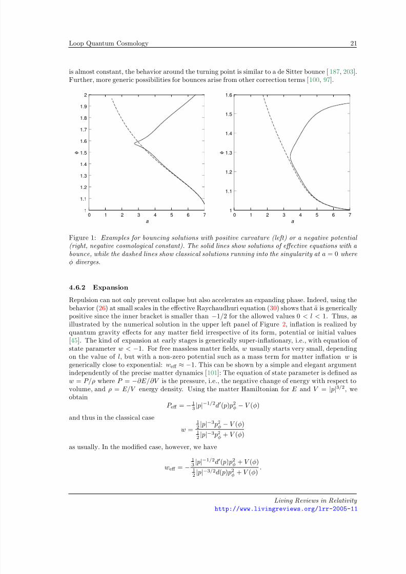
is almost constant, the behavior around the turning point is similar to a de Sitter bounce [ 187, 203].Further, more generic possibilities for bounces arise from other correction terms [100, 97].
0 1 2 3 4 5 6 7
a
1
1.1
1.2
1.3
1.4
1.5
1.6
1.7
1.8
1.9
2
φ
0 1 2 3 4 5 6 7
a
1
1.1
1.2
1.3
1.4
1.5
1.6
φ
Figure 1: Examples for bouncing solutions with positive curvature (left) or a negative potential (right, negative cosmological constant). The solid lines show solutions of effective equations with a bounce, while the dashed lines show classical solutions running into the singularity at a = 0 whereφ diverges.
4.6.2 Expansion
Repulsion can not only prevent collapse but also accelerates an expanding phase. Indeed, using thebehavior (26) at small scales in the effective Raychaudhuri equation (30) shows that a is genericallypositive since the inner bracket is smaller than −1/2 for the allowed values 0 < l < 1. Thus, asillustrated by the numerical solution in the upper left panel of Figure 2, inflation is realized byquantum gravity effects for any matter field irrespective of its form, potential or initial values[45]. The kind of expansion at early stages is generically super-inflationary, i.e., with equation of state parameter w < −1. For free massless matter fields, w usually starts very small, dependingon the value of l, but with a non-zero potential such as a mass term for matter inflation w isgenerically close to exponential: weff ≈ −1. This can be shown by a simple and elegant argumentindependently of the precise matter dynamics [101]: The equation of state parameter is defined asw = P/ρ where P = −∂E/∂V is the pressure, i.e., the negative change of energy with respect tovolume, and ρ = E/V energy density. Using the matter Hamiltonian for E and V = | p|3/2, weobtain
P eff = − 13| p|−1/2d( p) p2
φ − V (φ)
and thus in the classical case
w =12| p|−3 p2
φ − V (φ)12| p|−3 p2
φ + V (φ)
as usually. In the modified case, however, we have
weff = −13| p|−1/2d( p) p2
φ + V (φ)12| p|−3/2d( p) p2
φ + V (φ).
Living Reviews in Relativity http://www.livingreviews.org/lrr-2005-11
8/3/2019 Martin Bojowald- Loop Quantum Cosmology
http://slidepdf.com/reader/full/martin-bojowald-loop-quantum-cosmology 22/99
22 Martin Bojowald
0
0.5
φ
0 100 5000 10000t
0
5
10
a
a/ 300
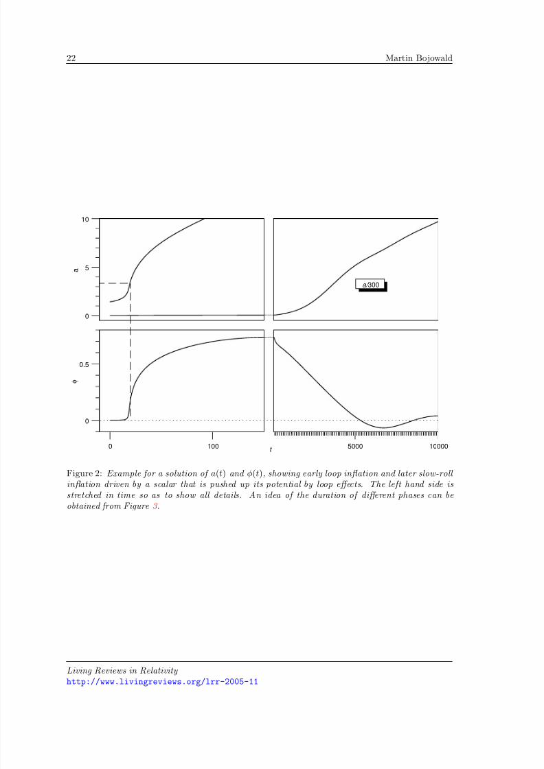
Figure 2: Example for a solution of a(t) and φ(t), showing early loop inflation and later slow-roll inflation driven by a scalar that is pushed up its potential by loop effects. The left hand side isstretched in time so as to show all details. An idea of the duration of different phases can beobtained from Figure 3 .
Living Reviews in Relativity http://www.livingreviews.org/lrr-2005-11
8/3/2019 Martin Bojowald- Loop Quantum Cosmology
http://slidepdf.com/reader/full/martin-bojowald-loop-quantum-cosmology 23/99
Loop Quantum Cosmology 23
V (φ)
a (t ) φ(t )
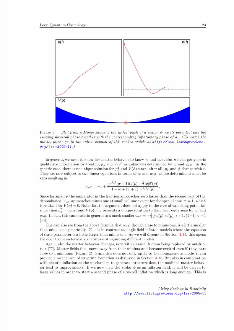
Figure 3: Still from a Movie showing the initial push of a scalar φ up its potential and theensuing slow-roll phase together with the corresponding inflationary phase of a. (To watch themovie, please go to the online version of this review article at http: //www.livingreviews.org/lrr-2005-11 .)
In general, we need to know the matter behavior to know w and weff . But we can get genericqualitative information by treating pφ and V (φ) as unknowns determined by w and weff . In thegeneric case, there is no unique solution for p2
φ and V (φ) since, after all, pφ and φ change with t.
They are now subject to two linear equations in terms of w and weff , whose determinant must bezero resulting in
weff = −1 +| p|3/2(w + 1)(d( p) − 2
3| p|d( p))
1 − w + (w + 1)| p|3/2d( p).
Since for small p the numerator in the fraction approaches zero faster than the second part of thedenominator, weff approaches minus one at small volume except for the special case w = 1, whichis realized for V (φ) = 0. Note that the argument does not apply to the case of vanishing potentialsince then p2
φ = const and V (φ) = 0 presents a unique solution to the linear equations for w and
weff . In fact, this case leads in general to a much smaller weff = − 23| p|d( p)/d( p) ≈ −1/(1− l) < −1
[45].
One can also see from the above formula that weff , though close to minus one, is a little smallerthan minus one generically. This is in contrast to single field inflaton models where the equationof state parameter is a little larger than minus one. As we will discuss in Section 4.15, this opensthe door to characteristic signatures distinguishing different models.
Again, also the matter behavior changes, now with classical friction being replaced by antifric-tion [77]. Matter fields thus move away from their minima and become excited even if they startclose to a minimum (Figure 2). Since this does not only apply to the homogeneous mode, it canprovide a mechanism of structure formation as discussed in Section 4.15. But also in combinationwith chaotic inflation as the mechanism to generate structure does the modified matter behav-ior lead to improvements: If we now view the scalar φ as an inflaton field, it will be driven tolarge values in order to start a second phase of slow-roll inflation which is long enough. This is
Living Reviews in Relativity http://www.livingreviews.org/lrr-2005-11
8/3/2019 Martin Bojowald- Loop Quantum Cosmology
http://slidepdf.com/reader/full/martin-bojowald-loop-quantum-cosmology 24/99
24 Martin Bojowald
satisfied for a large range of the ambiguity parameters j and l [67] and can even leave signatures[197] in the cosmic microwave spectrum [134]: The earliest moments when the inflaton starts toroll down its potential are not slow roll, as can also be seen in Figures 2 and 3 where the initialdecrease is steeper. Provided the resulting structure can be seen today, i.e., there are not toomany e-foldings from the second phase, this can lead to visible effects such as a suppression of power. Whether or not those effects are to be expected, i.e., which magnitude of the inflaton isgenerically reached by the mechanism generating initial conditions, is currently being investigatedat the basic level of loop quantum cosmology [27]. They should be regarded as first suggestions,indicating the potential of quantum cosmological phenomenology, which have to be substantiatedby detailed calculations including inhomogeneities or at least anisotropic geometries. In particularthe suppression of power can be obtained by a multitude of other mechanisms.
4.6.3 Model building
It is already clear that there are different inflationary scenarios using effects from loop cosmology. Ascenario without inflaton is more attractive since it requires less choices and provides a fundamental
explanation of inflation directly from quantum gravity. However, it is also more difficult to analyzestructure formation in this context while there are already well-developed techniques in slow rolescenarios.
In these cases where one couples loop cosmology to an inflaton model one still requires thesame conditions for the potential, but generically gets the required large initial values for thescalar by antifriction. On the other hand, finer details of the results now depend on the ambiguityparameters, which describe aspects of the quantization that also arise in the full theory.
It is also possible to combine collapsing and expanding phases in cyclic or oscillatory models[148]. One then has a history of many cycles separated by bounces, whose duration depends ondetails of the model such as the potential. There can then be many brief cycles until eventually, if the potential is right, one obtains an inflationary phase if the scalar has grown high enough. In thisway, one can develop ideas for the pre-history of our universe before the Big Bang. There are alsopossibilities to use a bounce to describe the structure in the universe. So far, this has only been
described in effective models [137] using brane scenarios [151] where the classical singularity hasbeen assumed to be absent by yet to be determined quantum effects. As it turns out, the explicitmechanism removing singularities in loop cosmology is not compatible with the assumptions madein those effective pictures. In particular, the scalar was supposed to turn around during the bounce,which is impossible in loop scenarios unless it encounters a range of positive potential during itsevolution [68]. Then, however, generically an inflationary phase commences as in [148], which isthen the relevant regime for structure formation. This shows how model building in loop cosmologycan distinguish scenarios that are more likely to occur from quantum gravity effects.
Cyclic models can be argued to shift the initial moment of a universe in the infinite past, butthey do not explain how the universe started. An attempt to explain this is the emergent universemodel [110, 112] where one starts close to a static solution. This is difficult to achieve classically,however, since the available fixed points of the equations of motion are not stable and thus a
universe departs too rapidly. Loop cosmology, on the other hand, implies an additional fixed pointof the effective equations which is stable and allows to start the universe in an initial phase of oscillations before an inflationary phase is entered [160, 53]. This presents a natural realization of the scenario where the initial scale factor at the fixed point is automatically small so as to startthe universe close to the Planck phase.
4.6.4 Stability
Cosmological equations displaying super-inflation or antifriction are often unstable in the sensethat matter can propagate faster than light. This has been voiced as a potential danger for loop
Living Reviews in Relativity http://www.livingreviews.org/lrr-2005-11
8/3/2019 Martin Bojowald- Loop Quantum Cosmology
http://slidepdf.com/reader/full/martin-bojowald-loop-quantum-cosmology 25/99
Loop Quantum Cosmology 25
cosmology, too [94, 95]. An analysis requires inhomogeneous techniques at least at an effectivelevel, such as those described in Section 4.12. It has been shown that loop cosmology is free of this problem, because the modified behavior for the homogeneous mode of the metric and matteris not relevant for matter propagation [129]. The whole cosmological picture that follows from theeffective equations is thus consistent.
4.7 Anisotropies
Anisotropic models provide a first generalization of isotropic ones to more realistic situations.They thus can be used to study the robustness of effects analyzed in isotropic situations and, atthe same time, provide a large class of interesting applications. An analysis in particular of thesingularity issue is important since the classical approach to a singularity can be very differentfrom the isotropic one. On the other hand, the anisotropic approach is deemed to be characteristiceven for general inhomogeneous singularities if the BKL scenario [31] is correct.
A general homogeneous but anisotropic metric is of the form
ds2 = −N (t)2 dt2 +
3I,J =1
qIJ (t)ωI ⊗ ωJ
with left-invariant 1-forms ωI on space Σ, which, thanks to homogeneity, can be identified withthe simply transitive symmetry group S as a manifold. The left-invariant 1-forms satisfy theMaurer–Cartan relations
dωI = −1
2C I JKωJ ∧ ωK
with the structure constants C I JK of the symmetry group. In a matrix parameterization of thesymmetry group, one can derive explicit expressions for ωI from the Maurer–Cartan form ωI T I =θMC = g−1dg with generators T I of S .
The simplest case of a symmetry group is an Abelian one with C I JK = 0, corresponding to theBianchi I model. In this case, S is given by R3 or a torus, and left-invariant 1-forms are simplyωI = dxI in Cartesian coordinates. Other groups must be restricted to class A models in thiscontext, satisfying C I JI = 0 since otherwise there is no Hamiltonian formulation. The structureconstants can then be parameterized as C I JK = I JK n(I ).
A common simplification is to assume the metric to be diagonal at all times, which correspondsto a reduction technically similar to a symmetry reduction. This amounts to qIJ = a2
(I )δIJ as wellas K IJ = K (I )δIJ for the extrinsic curvature with K I = aI . Depending on the structure constants,there is also non-zero intrinsic curvature quantified by the spin connection components
ΓI =1
2
aJ aK
nJ +aKaJ
nK − a2I
aJ aKnI
for IJK = 1. (33)
This influences the evolution as follows from the Hamiltonian constraint
− 18πG
a1a2a3 + a2a1a2 + a3a1a2 − (Γ2Γ3 − n1Γ1)a1 − (Γ1Γ3 − n2Γ2)a2
− (Γ1Γ2 − n3Γ3)a3
+ H matter(aI ) = 0. (34)
In the vacuum Bianchi I case the resulting equations are easy to solve by aI ∝ tαI withI αI =
I α
2I = 1 [135]. The volume a1a2a3 ∝ t vanishes for t = 0 where the classical singularity
appears. Since one of the exponents αI must be negative, however, only two of the aI vanish atthe classical singularity while the third one diverges. This already demonstrates how different thebehavior can be from the isotropic one and that anisotropic models provide a crucial test of anymechanism for singularity resolution.
Living Reviews in Relativity http://www.livingreviews.org/lrr-2005-11
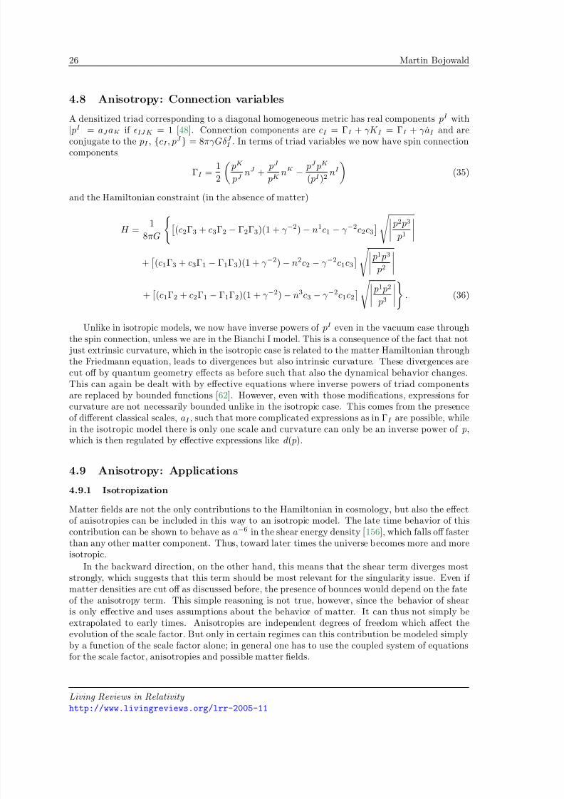
8/3/2019 Martin Bojowald- Loop Quantum Cosmology
http://slidepdf.com/reader/full/martin-bojowald-loop-quantum-cosmology 26/99
26 Martin Bojowald
4.8 Anisotropy: Connection variables
A densitized triad corresponding to a diagonal homogeneous metric has real components pI with
| pI
|= aJ aK if IJK = 1 [48]. Connection components are cI = ΓI + γK I = ΓI + γ aI and are
conjugate to the pI , cI , pJ = 8πγGδJ I . In terms of triad variables we now have spin connectioncomponents
ΓI =1
2
pK
pJ nJ +
pJ
pKnK − pJ pK
( pI )2nI
(35)
and the Hamiltonian constraint (in the absence of matter)
H =1
8πG
(c2Γ3 + c3Γ2 − Γ2Γ3)(1 + γ −2) − n1c1 − γ −2c2c3
p2 p3
p1
+
(c1Γ3 + c3Γ1 − Γ1Γ3)(1 + γ −2) − n2c2 − γ −2c1c3
p1 p3
p2
+
(c1Γ2 + c2Γ1 − Γ1Γ2)(1 + γ −2) − n3c3 − γ −2c1c2
p1 p2
p3
. (36)
Unlike in isotropic models, we now have inverse powers of pI even in the vacuum case throughthe spin connection, unless we are in the Bianchi I model. This is a consequence of the fact that not just extrinsic curvature, which in the isotropic case is related to the matter Hamiltonian throughthe Friedmann equation, leads to divergences but also intrinsic curvature. These divergences arecut off by quantum geometry effects as before such that also the dynamical behavior changes.This can again be dealt with by effective equations where inverse powers of triad componentsare replaced by bounded functions [62]. However, even with those modifications, expressions forcurvature are not necessarily bounded unlike in the isotropic case. This comes from the presence
of different classical scales, aI , such that more complicated expressions as in ΓI are possible, whilein the isotropic model there is only one scale and curvature can only be an inverse power of p,which is then regulated by effective expressions like d( p).
4.9 Anisotropy: Applications
4.9.1 Isotropization
Matter fields are not the only contributions to the Hamiltonian in cosmology, but also the effectof anisotropies can be included in this way to an isotropic model. The late time behavior of thiscontribution can be shown to behave as a−6 in the shear energy density [156], which falls off fasterthan any other matter component. Thus, toward later times the universe becomes more and moreisotropic.
In the backward direction, on the other hand, this means that the shear term diverges moststrongly, which suggests that this term should be most relevant for the singularity issue. Even if matter densities are cut off as discussed before, the presence of bounces would depend on the fateof the anisotropy term. This simple reasoning is not true, however, since the behavior of shearis only effective and uses assumptions about the behavior of matter. It can thus not simply beextrapolated to early times. Anisotropies are independent degrees of freedom which affect theevolution of the scale factor. But only in certain regimes can this contribution be modeled simplyby a function of the scale factor alone; in general one has to use the coupled system of equationsfor the scale factor, anisotropies and possible matter fields.
Living Reviews in Relativity http://www.livingreviews.org/lrr-2005-11
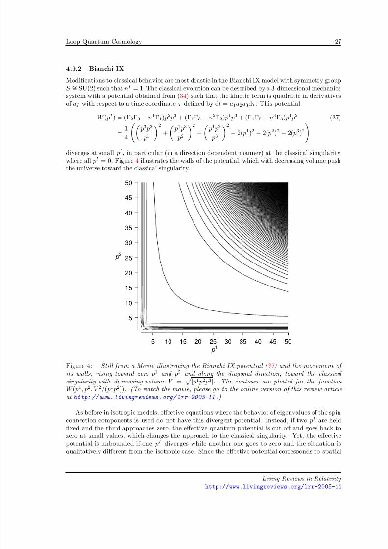
8/3/2019 Martin Bojowald- Loop Quantum Cosmology
http://slidepdf.com/reader/full/martin-bojowald-loop-quantum-cosmology 27/99
Loop Quantum Cosmology 27
4.9.2 Bianchi IX
Modifications to classical behavior are most drastic in the Bianchi IX model with symmetry groupS ∼= SU(2) such that nI = 1. The classical evolution can be described by a 3-dimensional mechanics
system with a potential obtained from (34) such that the kinetic term is quadratic in derivativesof aI with respect to a time coordinate τ defined by dt = a1a2a3dτ . This potential
W ( pI ) = (Γ2Γ3 − n1Γ1) p2 p3 + (Γ1Γ3 − n2Γ2) p1 p3 + (Γ1Γ2 − n3Γ3) p1 p2 (37)
=1
4
p2 p3
p1
2
+
p1 p3
p2
2
+
p1 p2
p3
2
− 2( p1)2 − 2( p2)2 − 2( p3)2
diverges at small pI , in particular (in a direction dependent manner) at the classical singularitywhere all pI = 0. Figure 4 illustrates the walls of the potential, which with decreasing volume pushthe universe toward the classical singularity.
5
10
15
20
25
30
35
40
45
50
p 2
5 10 15 20 25 30 35 40 45 50
p 1
Figure 4: Still from a Movie illustrating the Bianchi IX potential ( 37 ) and the movement of its walls, rising toward zero p1 and p2 and along the diagonal direction, toward the classical
singularity with decreasing volume V = | p1
p
2
p
3
|. The contours are plotted for the function W ( p1, p2, V 2/( p1 p2)). (To watch the movie, please go to the online version of this review articleat http: //www.livingreviews.org/lrr-2005-11 .)
As before in isotropic models, effective equations where the behavior of eigenvalues of the spinconnection components is used do not have this divergent potential. Instead, if two pI are heldfixed and the third approaches zero, the effective quantum potential is cut off and goes back tozero at small values, which changes the approach to the classical singularity. Yet, the effectivepotential is unbounded if one pI diverges while another one goes to zero and the situation isqualitatively different from the isotropic case. Since the effective potential corresponds to spatial
Living Reviews in Relativity http://www.livingreviews.org/lrr-2005-11
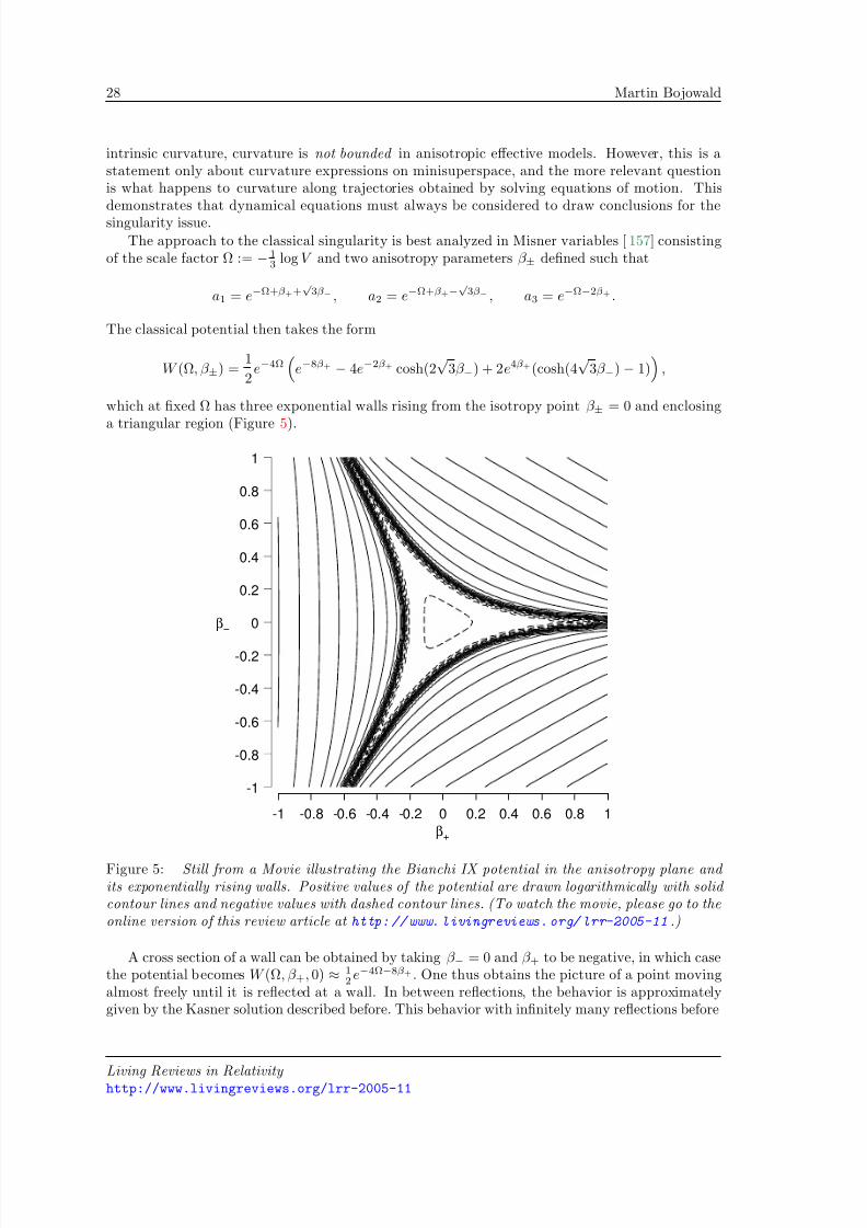
8/3/2019 Martin Bojowald- Loop Quantum Cosmology
http://slidepdf.com/reader/full/martin-bojowald-loop-quantum-cosmology 28/99
28 Martin Bojowald
intrinsic curvature, curvature is not bounded in anisotropic effective models. However, this is astatement only about curvature expressions on minisuperspace, and the more relevant questionis what happens to curvature along trajectories obtained by solving equations of motion. Thisdemonstrates that dynamical equations must always be considered to draw conclusions for thesingularity issue.
The approach to the classical singularity is best analyzed in Misner variables [ 157] consistingof the scale factor Ω := − 1
3 log V and two anisotropy parameters β ± defined such that
a1 = e−Ω+β++√
3β− , a2 = e−Ω+β+−√
3β− , a3 = e−Ω−2β+ .
The classical potential then takes the form
W (Ω, β ±) =1
2e−4Ω
e−8β+ − 4e−2β+ cosh(2
√3β −) + 2e4β+(cosh(4
√3β −) − 1)
,
which at fixed Ω has three exponential walls rising from the isotropy point β ± = 0 and enclosing
a triangular region (Figure 5).
-1
-0.8
-0.6
-0.4
-0.2
0
0.2
0.4
0.6
0.8
1
β−
-1 -0.8 -0.6 -0.4 -0.2 0 0.2 0.4 0.6 0.8 1
β+
Figure 5: Still from a Movie illustrating the Bianchi IX potential in the anisotropy plane and its exponentially rising walls. Positive values of the potential are drawn logarithmically with solid contour lines and negative values with dashed contour lines. (To watch the movie, please go to theonline version of this review article at http://www. livingreviews.org/ lrr-2005-11 .)
A cross section of a wall can be obtained by taking β − = 0 and β + to be negative, in which casethe potential becomes W (Ω, β +, 0) ≈ 1
2e−4Ω−8β+ . One thus obtains the picture of a point moving
almost freely until it is reflected at a wall. In between reflections, the behavior is approximatelygiven by the Kasner solution described before. This behavior with infinitely many reflections before
Living Reviews in Relativity http://www.livingreviews.org/lrr-2005-11
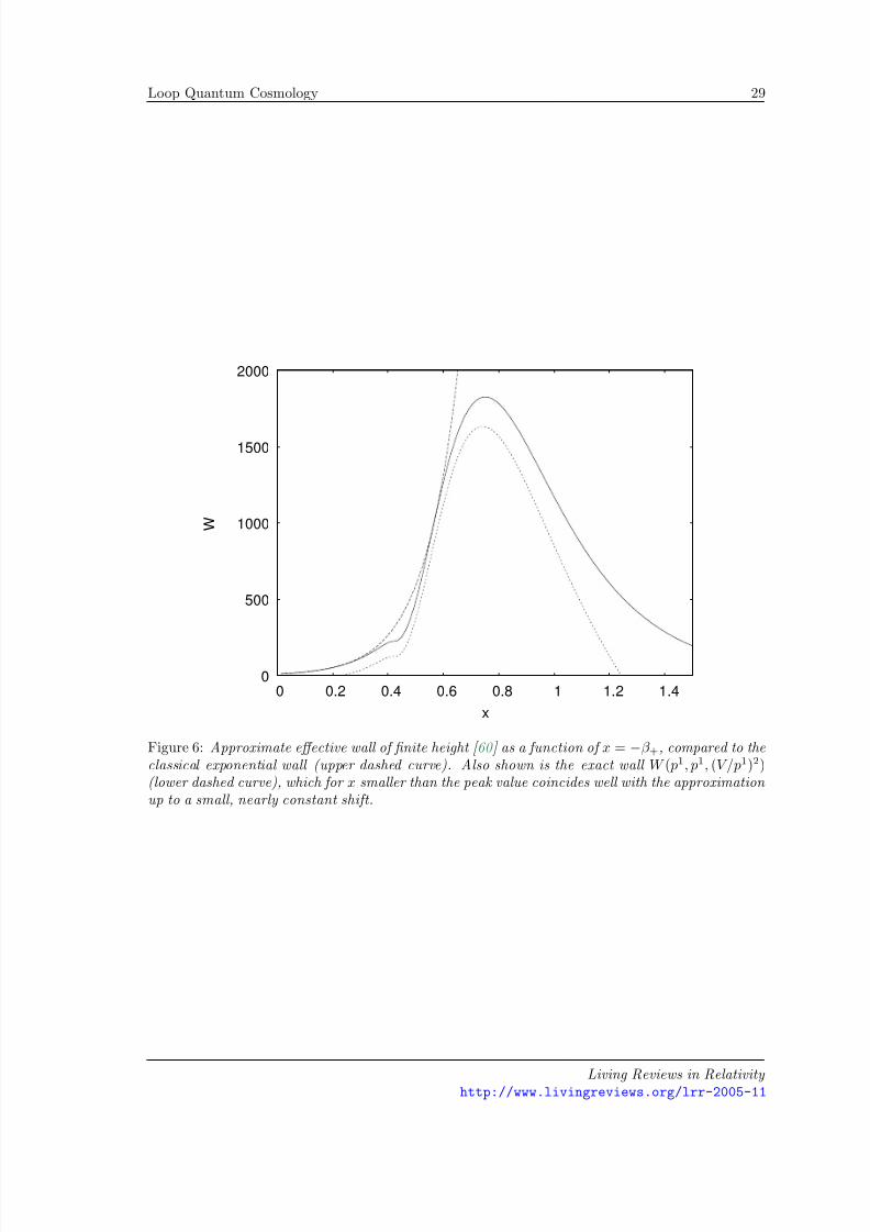
8/3/2019 Martin Bojowald- Loop Quantum Cosmology
http://slidepdf.com/reader/full/martin-bojowald-loop-quantum-cosmology 29/99
Loop Quantum Cosmology 29
0
500
1000
1500
2000
0 0.2 0.4 0.6 0.8 1 1.2 1.4
W
x
Figure 6: Approximate effective wall of finite height [ 60 ] as a function of x = −β +, compared to theclassical exponential wall (upper dashed curve). Also shown is the exact wall W ( p1, p1, (V /p1)2)(lower dashed curve), which for x smaller than the peak value coincides well with the approximation up to a small, nearly constant shift.
Living Reviews in Relativity http://www.livingreviews.org/lrr-2005-11
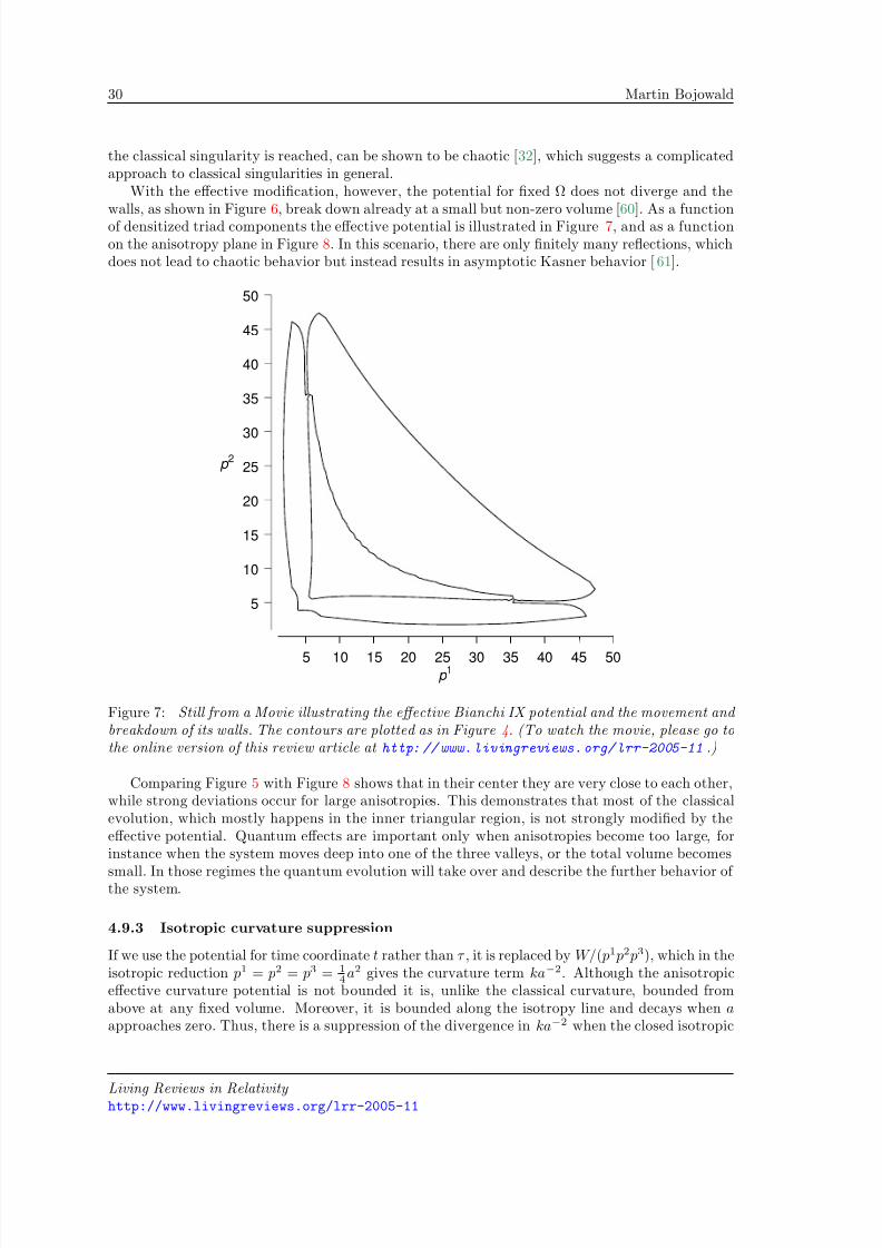
8/3/2019 Martin Bojowald- Loop Quantum Cosmology
http://slidepdf.com/reader/full/martin-bojowald-loop-quantum-cosmology 30/99
30 Martin Bojowald
the classical singularity is reached, can be shown to be chaotic [32], which suggests a complicatedapproach to classical singularities in general.
With the effective modification, however, the potential for fixed Ω does not diverge and thewalls, as shown in Figure 6, break down already at a small but non-zero volume [60]. As a functionof densitized triad components the effective potential is illustrated in Figure 7, and as a functionon the anisotropy plane in Figure 8. In this scenario, there are only finitely many reflections, whichdoes not lead to chaotic behavior but instead results in asymptotic Kasner behavior [ 61].
5
10
15
20
25
30
35
40
45
50
p 2
5 10 15 20 25 30 35 40 45 50
p 1
Figure 7: Still from a Movie illustrating the effective Bianchi IX potential and the movement and breakdown of its walls. The contours are plotted as in Figure 4. (To watch the movie, please go tothe online version of this review article at http: //www.livingreviews.org/lrr-2005-11 .)
Comparing Figure 5 with Figure 8 shows that in their center they are very close to each other,while strong deviations occur for large anisotropies. This demonstrates that most of the classicalevolution, which mostly happens in the inner triangular region, is not strongly modified by theeffective potential. Quantum effects are important only when anisotropies become too large, forinstance when the system moves deep into one of the three valleys, or the total volume becomes
small. In those regimes the quantum evolution will take over and describe the further behavior of the system.
4.9.3 Isotropic curvature suppression
If we use the potential for time coordinate t rather than τ , it is replaced by W/( p1 p2 p3), which in theisotropic reduction p1 = p2 = p3 = 1
4 a2 gives the curvature term ka−2. Although the anisotropiceffective curvature potential is not bounded it is, unlike the classical curvature, bounded fromabove at any fixed volume. Moreover, it is bounded along the isotropy line and decays when aapproaches zero. Thus, there is a suppression of the divergence in ka−2 when the closed isotropic
Living Reviews in Relativity http://www.livingreviews.org/lrr-2005-11
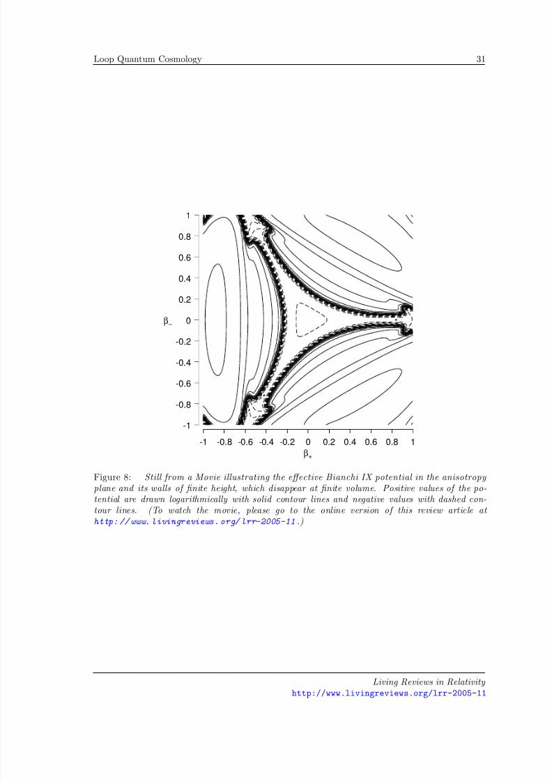
8/3/2019 Martin Bojowald- Loop Quantum Cosmology
http://slidepdf.com/reader/full/martin-bojowald-loop-quantum-cosmology 31/99
Loop Quantum Cosmology 31
-1
-0.8
-0.6
-0.4
-0.2
0
0.2
0.4
0.6
0.8
1
β−
-1 -0.8 -0.6 -0.4 -0.2 0 0.2 0.4 0.6 0.8 1
β+
Figure 8: Still from a Movie illustrating the effective Bianchi IX potential in the anisotropy plane and its walls of finite height, which disappear at finite volume. Positive values of the po-tential are drawn logarithmically with solid contour lines and negative values with dashed con-tour lines. (To watch the movie, please go to the online version of this review article at http://www. livingreviews.org/ lrr-2005-11 .)
Living Reviews in Relativity http://www.livingreviews.org/lrr-2005-11
8/3/2019 Martin Bojowald- Loop Quantum Cosmology
http://slidepdf.com/reader/full/martin-bojowald-loop-quantum-cosmology 32/99
32 Martin Bojowald
model is viewed as embedded in a Bianchi IX model. Similarly to matter Hamiltonians, intrinsiccurvature then approaches zero at zero scale factor.
This is a further illustration for the special nature of isotropic models compared to anisotropicones. In the classical reduction, the pI in the anisotropic spin connection cancel such that the spinconnection is a constant and no special steps are needed for its quantization. By viewing isotropicmodels within anisotropic ones, one can consistently realize the model and see a suppression of intrinsic curvature terms. Anisotropic models, on the other hand, do not have, and do not need,complete suppression since curvature functions can still be unbounded.
4.10 Anisotropy: Implications for inhomogeneities
Even without implementing inhomogeneous models the previous discussion allows some tentativeconclusions as to the structure of general singularities. This is based on the BKL picture [ 31] whosebasic idea is to study Einstein’s field equations close to a singularity. One can then argue thatspatial derivatives become subdominant compared to time-like derivatives such that the approachshould locally be described by homogeneous models, in particular the Bianchi IX model since it
has the most freedom in its general solution.Since spatial derivatives are present, though, they lead to small corrections and couple the
geometries in different spatial points. One can visualize this by starting with an initial slicewhich is approximated by a collection of homogeneous patches. For some time, each patch evolvesindependently of the others, but this is not precisely true since coupling effects have been ignored.Moreover, each patch geometry evolves in a chaotic manner, which means that two initially nearbygeometries depart rapidly from each other. The approximation can thus be maintained only if thepatches are subdivided during the evolution, which goes on without limits in the approach to thesingularity. There is, thus, more and more inhomogeneous structure being generated on arbitrarilysmall scales, which leads to a complicated picture of a general singularity.
This picture can be taken over to the effective behavior of the Bianchi IX model. Here, thepatches do not evolve chaotically even though at larger volume they follow the classical behavior.
The subdivision thus has to be done also for the initial effective evolution. At some point, however,when reflections on the potential walls stop, the evolution simplifies and subdivisions are no longernecessary. There is thus a lower bound to the scale of structure whose precise value depends on theinitial geometries. Nevertheless, from the scale at which the potential walls break down one canshow that structure formation stops at the latest when the discreteness scale of quantum geometryis reached [60]. This can be seen as a consistency test of the theory since structure below thediscreteness could not be supported by quantum geometry.
We have thus a glimpse on the inhomogeneous situation with a complicated but consistentapproach to a general classical singularity. The methods involved, however, are not very robustsince the BKL scenario, which even classically is still at the level of a conjecture for the generalcase [32, 168], would need to be available as an approximation to quantum geometry. For morereliable results the methods need to be refined to take into account inhomogeneities properly.
4.11 Inhomogeneities
Allowing for inhomogeneities inevitably means to take a big step from finitely many degrees of freedom to infinitely many ones. There is no straightforward way to cut down the number of degreesof freedom to finitely many ones while being more general than in the homogeneous context. Onepossibility would be to introduce a small-scale cut-off such that only finitely many wave modesarise (e.g., through a lattice as is indeed done in some coherent state constructions [184]). This isin fact expected to happen in a discrete framework such as quantum geometry, but would at thisstage of defining a model simply be introduced by hand.
Living Reviews in Relativity http://www.livingreviews.org/lrr-2005-11
8/3/2019 Martin Bojowald- Loop Quantum Cosmology
http://slidepdf.com/reader/full/martin-bojowald-loop-quantum-cosmology 33/99
Loop Quantum Cosmology 33
For the analysis of inhomogeneous situations there are several different approximation schemes:
• Use only isotropic quantum geometry and in particular its effective description, but couple
to inhomogeneous matter fields. Problems in this approach are that back-reaction effects areignored (which is also the case in most classical treatments) and that there is no direct wayhow to check modifications used in particular for gradient terms of the matter Hamiltonian.So far, this approach has led to a few indications of possible effects.
• Start with the full constraint operator, write it as the homogeneous one plus correctionterms from inhomogeneities, and derive effective classical equations. This approach is moreambitious since contact to the full theory is realized. So far, there are not many results sincea suitable perturbation scheme has to be developed.
• There are inhomogeneous symmetric models, such as Einstein–Rosen waves or the sphericallysymmetric one, which have infinitely many kinematical degrees of freedom but can be treated
explicitly. Also here, contact to the full theory is present through the symmetry reductionprocedure of Section 6. This procedure itself can be tested by studying those models betweenhomogeneous ones and the full theory, but results can also be used for physical applicationsinvolving inhomogeneities. Many issues that are of importance in the full theory, such as theanomaly problem, also arise here and can thus be studied more explicitly.
4.12 Inhomogeneous matter with isotropic quantum geometry
Inhomogeneous matter fields cannot be introduced directly to isotropic quantum geometry sinceafter the symmetry reduction there is no space manifold left for the fields to live on. There are thentwo different routes to proceed: One can simply take the classical field Hamiltonian and introduceeffective modifications modeled on what happens to the isotropic Hamiltonian, or perform a modedecomposition of the matter fields and just work with the space-independent amplitudes. The latteris possible since the homogeneous geometry provides a background for the mode decomposition.
The basic question, for the example of a scalar field, then is how the metric coefficient in thegradient term of Equation (12), E ai E bi /
|det E |, would be replaced effectively. For the other terms,
one can simply use the isotropic modification, which is taken directly from the quantization. For thegradient term, however, one does not have a quantum expression in this context and a modificationcan only be guessed. The problem arises since the inhomogeneous term involves inverse powers of E , while in the isotropic context the coefficient just reduces to
| p|, which would not be modified
at all. There is thus no obvious and unique way to find a suitable replacement.
A possible route would be to read off the modification from the full quantum Hamiltonian, or atleast from an inhomogeneous model, which requires a better knowledge of the reduction procedure.Alternatively, one can take a more phenomenological point of view and study the effects of possiblereplacements. If the robustness of these effects to changes in the replacements is known, one canget a good picture of possible implications. So far, only initial steps have been taken and there isno complete programme in this direction.
Another approximation of the inhomogeneous situation has been developed in [ 70] by patchingisotropic quantum geometries together to support an inhomogeneous matter field. This can beused to study modified dispersion relations to the extent that the result agrees with preliminarycalculations performed in the full theory [115, 3, 4, 181, 182] even at a quantitative level. There isthus further evidence that symmetric models and their approximations can provide reliable insightsinto the full theory.
Living Reviews in Relativity http://www.livingreviews.org/lrr-2005-11
8/3/2019 Martin Bojowald- Loop Quantum Cosmology
http://slidepdf.com/reader/full/martin-bojowald-loop-quantum-cosmology 34/99
34 Martin Bojowald
4.13 Inhomogeneity: Perturbations
With a symmetric background, a mode decomposition is not only possible for matter fields but alsofor geometry. The homogeneous modes can then be quantized as before, while higher modes are
coupled as perturbations implementing inhomogeneities [120]. As with matter Hamiltonians before,one can then also deal with the gravitational part of the Hamiltonian constraint. In particular,there are terms with inverse powers of the homogeneous fields which receive modifications uponquantization. As with gradient terms in matter Hamiltonians, there are several options for thosemodifications which can only be restricted by relating them to the full Hamiltonian. This wouldrequire introducing the mode decomposition, analogously to symmetry conditions, at the quantumlevel and writing the full constraint operator as the homogeneous one plus correction terms.
An additional complication compared to matter fields is that one is now dealing with infinitelymany coupled constraint equations since the lapse function N (x) is inhomogeneous, too. Thisfunction can itself be decomposed into modes
n N nY n(x), with harmonics Y n(x) according to
the symmetry, and each amplitude N n is varied independently giving rise to a separate constraint.The main constraint arises from the homogeneous mode, which describes how inhomogeneities
affect the evolution of the homogeneous scale factors.
4.14 Inhomogeneous models
The full theory is complicated at several different levels of both conceptual and technical na-ture. For instance, one has to deal with infinitely many degrees of freedom, most operators havecomplicated actions, and interpreting solutions to all constraints in a geometrical manner can bedifficult. Most of these complications are avoided in homogeneous models, in particular when ef-fective classical equations are employed. These equations use approximations of expectation valuesof quantum geometrical operators which need to be known rather explicitly. The question thenarises whether one can still work at this level while relaxing the symmetry conditions and bringingin more complications of the full theory.
Explicit calculations at a level similar to homogeneous models, at least for matrix elements
of individual operators, are possible in inhomogeneous models, too. In particular the sphericallysymmetric model and cylindrically symmetric Einstein–Rosen waves are of this class, where thesymmetry or other conditions are strong enough to result in a simple volume operator. In thespherically symmetric model, this simplification comes from the remaining isotropy subgroup iso-morphic to U(1) in generic points, while the Einstein–Rosen model is simplified by polarizationconditions that play a role analogous to the diagonalization of homogeneous models. With thesemodels one obtains access to applications for black holes and gravitational waves, but also toinhomogeneities in cosmology.
In spherical coordinates x, ϑ, ϕ a spherically symmetric spatial metric takes the form
ds2 = qxx(x, t) dx2 + qϕϕ(x, t) dΩ2
with dΩ2 = dϑ2 + sin2 ϑ dϕ2. This is related to densitized triad components by [196, 136]
|E x| = qϕϕ, (E ϕ)2 = qxxqϕϕ,
which are conjugate to the other basic variables given by the Ashtekar connection component Ax
and the extrinsic curvature component K ϕ:
Ax(x), E x(y) = 8πGγδ(x, y), γK ϕ(x), E ϕ(y) = 16πGγδ(x, y).
Note that we use the Ashtekar connection for the inhomogeneous direction x but extrinsic curvaturefor the homogeneous direction along symmetry orbits [75]. Connection and extrinsic curvature
Living Reviews in Relativity http://www.livingreviews.org/lrr-2005-11
8/3/2019 Martin Bojowald- Loop Quantum Cosmology
http://slidepdf.com/reader/full/martin-bojowald-loop-quantum-cosmology 35/99
Loop Quantum Cosmology 35
components for the ϕ-direction are related by A2ϕ = Γ2
ϕ+γ 2K 2ϕ with the spin connection component
Γϕ = − E x
2E ϕ. (38)
Unlike in the full theory or homogeneous models, Aϕ is not conjugate to a triad component but to[52]
P ϕ =
4(E ϕ)2 − A−2
ϕ (P β)2
with the momentum P β conjugate to a U(1)-gauge angle β . This is a rather complicated functionof both triad and connection variables such that the volume V = 4π
|E x|E ϕdx would have arather complicated quantization. It would still be possible to compute the full volume spectrum,but with the disadvantage that volume eigenstates would not be given by triad eigenstates such thatcomputations of many operators would be complicated [74]. This can be avoided by using extrinsiccurvature which is conjugate to the triad component [75]. Moreover, this is also in accordancewith a general scheme to construct Hamiltonian constraint operators for the full theory as well assymmetric models [194, 42, 58].
The constraint operator in spherical symmetry is given by
H [N ] = −(2G)−1
B
dxN (x)|E x|−1/2
(K 2ϕE ϕ + 2K ϕK xE x) + (1 − Γ2ϕ)E ϕ + 2ΓϕE x
(39)
accompanied by the diffeomorphism constraint
D[N x] = (2G)−1
B
N x(x)(2E ϕK ϕ − K xE x). (40)
We have expressed this in terms of K x for simplicity, keeping in mind that as the basic variablefor quantization we will later use the connection component Ax.
Since the Hamiltonian constraint contains the spin connection component Γϕ given by (38),
which contains inverse powers of densitized triad components, one can expect effective classicalequations with modifications similar to the Bianchi IX model. However, the situation is now muchmore complicated since we have a system constrained by many constraints with a non-Abelianalgebra. Simply replacing the inverse of E ϕ with a bounded function as before will change theconstraint algebra and thus most likely lead to anomalies. It is currently open if a more refinedreplacement can be done where not only the spin connection but also the extrinsic curvature termsare modified. This issue has the potential to shed light on many questions related to the anomalyissue. It is one of the cases where models between homogeneous ones, where the anomaly problemtrivializes, and the full theory are most helpful.
4.15 Inhomogeneity: Results
There are some results obtained for inhomogeneous systems. We have already discussed glimpsesfrom the BKL picture, which used loop results only for anisotropic models. Methods described inthis section have led to some preliminary insights into possible cosmological scenarios.
4.15.1 Matter gradient terms and small-a effects
When an inhomogeneous matter Hamiltonian is available it is possible to study its implicationson the cosmic microwave background with standard techniques. With modifications of densitiesthere are then different regimes since the part of the inflationary era responsible for the formationof currently visible structure can be in the small-a or large-a region of the effective density.
Living Reviews in Relativity http://www.livingreviews.org/lrr-2005-11
8/3/2019 Martin Bojowald- Loop Quantum Cosmology
http://slidepdf.com/reader/full/martin-bojowald-loop-quantum-cosmology 36/99
36 Martin Bojowald
The small-a regime below the peak of effective densities has more dramatic effects since inflationcan here be provided by quantum geometry effects alone and the matter behavior changes to beanti-frictional [45, 77]. Mode evolution in this regime has been investigated for a particular choiceof gradient term and using a power-law approximation for the effective density at small a, with theresult that there are characteristic signatures [130]. As in standard inflation models the spectrumis nearly scale invariant, but its spectral index is slightly larger than one (blue tilt) as comparedto slightly smaller than one (red tilt) for single-field inflaton models. Since small scale factors atearly stages of inflation generate structure which today appears on the largest scales, this impliesthat low multipoles of the power spectrum should have a blue tilt. The running of the spectralindex in this regime can also be computed but depends only weakly on ambiguity parameters.
The main parameter then is the duration of loop inflation. In the simplest scenario, one canassume only one inflationary phase, which would require huge values for the ambiguity parameter j. This is unnatural and would imply that the spectrum is blue on almost all scales, which isin conflict with present observations. Thus, not only conceptual arguments but also cosmologicalobservations point to smaller values for j, which is quite remarkable.
In order to have sufficient inflation to make the universe big enough one then needs additional
stages provided by the behavior of matter fields. One still does not need an inflaton since now thedetails of the expansion after the structure generating phase are less important. Any matter fieldbeing driven away from its potential minimum during loop inflation and rolling down its potentialthereafter suffices. Depending on the complexity of the model there can be several such phases.
4.15.2 Matter gradient terms and large-a effects
At larger scale factors above the peak of effective densities there are only perturbative correctionsfrom loop effects. This has been investigated with the aim of finding trans-Planckian corrections tothe microwave background, also here with a particular gradient term. In this model, cancellationshave been observed that imply that corrections appear only at higher orders of the perturbationseries and are too weak to be observable [126].
A common problem of both analyses is that the robustness of the observed effects has not yetbeen studied. This is in particular a pressing problem since one modification of the gradient termhas been chosen without further motivation. Moreover, the modifications in both examples weredifferent. Without a more direct derivation of the modifications from inhomogeneous models orthe full theory one can only rely on a robustness analysis to show that the effects can be trusted.In particular the cancellation in the second example must be shown to be realized for a larger classof modifications.
4.15.3 Non-inflationary structure formation
Given a modification of the gradient term, one obtains effective equations for the matter field,which for a scalar results in a modified Klein–Gordon equation. After a mode decomposition, onecan then easily see that all the modes behave differently at small scales with the classical frictionreplaced by anti-friction as in Section 4.5. Thus, not only the average value of the field is drivenaway from its potential minimum but also higher modes are being excited. The coupled dynamicsof all the modes thus provides a scenario for structure formation, which does not rely on inflationbut on the anti-friction effect of loop cosmology.
Even though all modes experience this effect, they do not all see it in the same way. Thegradient term implies an additive contribution to the potential proportional to k2 for a mode of wave number k, which also depends on the metric in a way determined by the gradient termmodification. For larger scales, the additional term is not essential and their amplitudes willbe pushed to similar magnitudes, suggesting scale invariance for them. The potential relevant
Living Reviews in Relativity http://www.livingreviews.org/lrr-2005-11

8/3/2019 Martin Bojowald- Loop Quantum Cosmology
http://slidepdf.com/reader/full/martin-bojowald-loop-quantum-cosmology 37/99
Loop Quantum Cosmology 37
for higher modes, however, becomes steeper and steeper such that they are less excited by anti-friction and retain a small initial amplitude. In this way, the structure formation scenario providesa dynamical mechanism for a small-scale cut-off, possibly realizing older expectations [165, 166].
4.15.4 Stability
As already noted, inhomogeneous matter Hamiltonians can be used to study the stability of cos-mological equations in the sense that matter does not propagate faster than light. The modifiedbehavior of homogeneous modes has led to the suspicion that loop cosmology is not stable [ 94, 95]since other cosmological models displaying super-inflation have this problem. A detailed analy-sis of the loop equations, however, shows that the equations as they arise from modifications areautomatically stable. While the homogeneous modes display super-inflationary and anti-frictionalbehavior, they are not relevant for matter propagation. Modes relevant for propagation, on theother hand, are modified differently in such a manner that the total behavior is stable [129].Most importantly, this is an example where an inhomogeneous matter Hamiltonian with its mod-ifications must be used and the qualitative result of stability can be shown to be robust under
possible changes of the effective modification. This shows that reliable conclusions can be drawnfor important issues without a precise definition of the effective inhomogeneous behavior.
4.16 Summary
Loop cosmology is an effective description of quantum effects in cosmology, obtained in a frameworkof a background independent and non-perturbative quantization. There is mainly one changecompared to classical equations coming from modified densities in matter Hamiltonians or alsoanisotropy potentials. These modifications are non-perturbative as they contain inverse powers of the Planck length and thus the gravitational constant, but also perturbative corrections arise fromcurvature terms, which are now being studied.
The non-perturbative modification alone is responsible for a surprising variety of phenomena,which all improve the behavior in classical cosmology. Nevertheless, the modification had not
been motivated by phenomenology but derived through the background independent quantization.Details of its derivation in cosmological models and its technical origin will now be reviewed inSection 5, before we come to a discussion of the link to the full theory in Section 6.
Living Reviews in Relativity http://www.livingreviews.org/lrr-2005-11
8/3/2019 Martin Bojowald- Loop Quantum Cosmology
http://slidepdf.com/reader/full/martin-bojowald-loop-quantum-cosmology 38/99
38 Martin Bojowald
5 Loop quantization of symmetric models
Analogies prove nothing, but they can make one feel more at home.Sigmund Freud
Introductory Lectures on Psychoanalysis
In full loop quantum gravity, the quantum representation is crucial for the foundation of thetheory. The guiding theme there is background independence, which requires one to smear thebasic fields in a particular manner to holonomies and fluxes. In this section, we will see whatimplications this has for composite operators and the physical effects they entail. We will base thisanalysis on symmetric models in order to be able to perform explicit calculations.
Symmetries are usually introduced in order to simplify calculations or make them possiblein the first place. However, symmetries can sometimes also lead to complications in conceptualquestions if the additional structure they provide is not fully taken into account. In the presentcontext, it is important to realize that the action of a symmetry group on a space manifold providesa partial background such that the situation is always slightly different from the full theory. If the
symmetry is strong, such as in homogeneous models, other representations such as the Wheeler–DeWitt representation can be possible even though the fact that a background has been usedmay not be obvious. While large scale physics is not very sensitive to the representation used,it becomes very important on the smallest scales, which we have to take into account when thesingularity issue is considered.
Instead of looking only at one symmetric model, where one may have different possibilities tochoose the basic representation, one should thus keep the full view on different models as well asthe full theory. In fact, in loop quantum gravity it is possible to relate models and the full theorysuch that symmetric states and basic operators, and thus the representation, can be derived fromthe unique background independent representation of the full theory. We will describe this in detailin Section 6, after having discussed the construction of quantum models in the present section.Without making use of the relation to the full theory, one can construct models by analogy . Thismeans that quantization steps are modeled on those which are known to be crucial in the full
theory, which starts with the basic representation and continues to the Hamiltonian constraintoperator. One can then disentangle places where additional input as compared to the full theoryis needed and which implications it has.
5.1 Symmetries and backgrounds
It is impossible to introduce symmetries in a completely background independent manner. Themathematical action of a symmetry group is defined by a mapping between abstract points, whichdo not exist in a diffeomorphism invariant setting (if one, for instance, considers only equivalenceclasses up to arbitrary diffeomorphisms).
More precisely, while the full theory has as background only a differentiable or analytic manifoldΣ, a symmetric model has as background a symmetric manifold (Σ, S ) consisting of a differentiable
or analytic manifold Σ together with an action of a symmetry group S : Σ → Σ. How strong theadditional structure is depends on the symmetry used. The strongest symmetry in gravitationalmodels is realized with spatial isotropy, which implies a unique spatial metric up to a scale factor.The background is thus equivalent to a conformal space.
All constructions in a given model must take its symmetry into account since otherwise itsparticular dynamics, for instance, could not be captured. The structure of models thus depends onthe different types of background realized for different symmetry groups. This can not only lead tosimplifications but also to conceptual differences, and it is always instructive to keep the completeview on different models as well as the full theory. Since the loop formalism is general enough toencompass all relevant models, there are many ways to compare and relate different systems. It is
Living Reviews in Relativity http://www.livingreviews.org/lrr-2005-11
8/3/2019 Martin Bojowald- Loop Quantum Cosmology
http://slidepdf.com/reader/full/martin-bojowald-loop-quantum-cosmology 39/99
Loop Quantum Cosmology 39
thus possible to observe characteristic features of (metric) background independence even in caseswhere more structure is available.
5.2 IsotropyIsotropic models are described purely in terms of the scale factor a(t) such that there is only asingle kinematical degree of freedom. In connection variables, this is parameterized by the triadcomponent p conjugate to the connection component c.
If we restrict ourselves to invariant connections of a given form, it suffices to probe them withonly special holonomies. For an isotropic connection Ai
a = cΛiI ω
I a (see Appendix B.2) we can
choose holonomies along one integral curve of a symmetry generator X I . They are of the form
hI = exp
AiaX aI τ i = cos 1
2µc + 2Λi
I τ i sin 12
µc (41)
where µ depends on the parameter length of the curve and can be any real number (thanks to
homogeneity, path ordering is not necessary). Since knowing the values cos1
2 µ and sin1
2 µc for allµ uniquely determines the value of c, which is the only gauge invariant information contained inthe connection, these holonomies describe the configuration space of connections completely.
This illustrates how symmetric configurations allow one to simplify the constructions behindthe full theory. But it also shows which effects the presence of a partial background can haveon the formalism [15]. In the present case, the background enters through the left-invariant 1-forms ωI defined on the spatial manifold whose influence is contained in the parameter µ. Allinformation about the edge used to compute the holonomy is contained in this single parameter,which leads to degeneracies compared to the full theory. Most importantly, one cannot distinguishbetween the parameter length and the spin label of an edge: Taking a power of the holonomy ina non-fundamental representation simply rescales µ, which could just as well come from a longerparameter length. That this is related to the presence of a background can be seen by looking at theroles of edges and spin labels in the full theory. There, both concepts are independent and appear
very differently. While the embedding of an edge, including its parameter length, is removed bydiffeomorphism invariance, the spin label remains well-defined and is important for ambiguities of operators. In the model, however, the full diffeomorphism invariance is not available such thatsome information about edges remains in the theory and merges with the spin label. Issues likethat have to be taken into account when constructing operators in a model and comparing withthe full theory.
The functions appearing in holonomies for isotropic connections define the algebra of functionson the classical configuration space which, together with fluxes, is to be represented on a Hilbertspace. This algebra does not contain arbitrary continuous functions of c but only almost periodicones of the form [15]
f (c) =
µf µ exp(iµc/2) (42)
where the sum is over a countable subset of R. This is analogous to the full situation, reviewed inSection 3.4, where matrix elements of holonomies define a special algebra of continuous functionsof connections. As in this case, the algebra can be represented as the set of all continuous functionson a compact space, called its spectrum. This compactification can be imagined as being obtainedfrom enlarging the classical configuration space R by adding points, and thus more continuityconditions, until only functions of the given algebra survive as continuous ones. A well-knownexample is the one point compactification, which is the spectrum of the algebra of continuousfunctions f for which limx→−∞ f (x) = limx→∞ f (x) exists. In this case, one just needs to add asingle point at infinity.
Living Reviews in Relativity http://www.livingreviews.org/lrr-2005-11
8/3/2019 Martin Bojowald- Loop Quantum Cosmology
http://slidepdf.com/reader/full/martin-bojowald-loop-quantum-cosmology 40/99
40 Martin Bojowald
In the present case, the procedure is more complicated and leads to the Bohr compactificationRBohr, which contains R densely. It is very different from the one point compactification, as can beseen from the fact that the only function which is continuous on both spaces is the zero function.In contrast to the one point compactification, the Bohr compactification is an Abelian group, justlike R itself. Moreover, there is a one-to-one correspondence between irreducible representationsof R and irreducible representations of RBohr, which can also be used as the definition of theBohr compactification. Representations of RBohr are thus labeled by real numbers and given byρµ : RBohr → C, c → eiµc. As with any compact group, there is a unique normalized Haar measuredµ(c) given by
RBohr
f (c) dµ(c) = limT →∞
1
2T
T −T
f (c) dc, (43)
where on the right hand side the Lebesgue measure on R is used.The Haar measure defines the inner product for the Hilbert space L2(RBohr, dµ(c)) of square
integrable functions on the quantum configuration space. As one can easily check, exponentials of the form c|µ = eiµc/2 are normalized and orthogonal to each other for different µ,
µ1|µ2 = δµ1,µ2 , (44)
which demonstrates that the Hilbert space is not separable.Similarly to holonomies, one needs to consider fluxes only for special surfaces, and all informa-
tion is contained in the single number p. Since it is conjugate to c, it is quantized to a derivativeoperator
ˆ p = −13 iγ2
P
d
dc, (45)
whose actionˆ p|µ = 1
6γ2
Pµ|µ =: pµ|µ (46)
on basis states |µ can easily be determined. In fact, the basis states are eigenstates of the fluxoperator, which demonstrates that the flux spectrum is discrete (all eigenstates are normalizable).
This property is analogous to the full theory with its discrete flux spectra, and similarly itimplies discrete quantum geometry. We thus see that the discreteness survives the symmetryreduction in this framework [37]. Similarly, the fact that only holonomies are represented in thefull theory but not connection components is realized in the model, too. In fact, we have so farrepresented only exponentials of c, and one can see that these operators are not continuous inthe parameter µ. Thus, an operator quantizing c directly does not exist on the Hilbert space.These properties are analogous to the full theory, but very different from the Wheeler–DeWittquantization. In fact, the resulting representations in isotropic models are inequivalent. While therepresentation is not of crucial importance when only small energies or large scales are involved[18], it becomes essential at small scales which are in particular realized in cosmology.
5.3 Isotropy: Matter Hamiltonian
We now know how the basic quantities p and c are quantized, and can use the operators to constructmore complicated ones. Of particular importance, also for cosmology, are matter Hamiltonianswhere now not only the matter field but also geometry is quantized. For an isotropic geometryand a scalar, this requires us to quantize | p|−3/2 for the kinetic term and | p|3/2 for the potentialterm. The latter can be defined readily as |ˆ p|3/2, but for the former we need an inverse power of p. Since ˆ p has a discrete spectrum containing zero, a densely defined inverse does not exist.
At this point, one has to find an alternative route to the quantization of d( p) = | p|−3/2, orelse one could only conclude that there is no well-defined quantization of matter Hamiltonians asa manifestation of the classical divergence. In the case of loop quantum cosmology it turns out,
Living Reviews in Relativity http://www.livingreviews.org/lrr-2005-11
8/3/2019 Martin Bojowald- Loop Quantum Cosmology
http://slidepdf.com/reader/full/martin-bojowald-loop-quantum-cosmology 41/99
Loop Quantum Cosmology 41
following a general scheme of the full theory [193], that one can reformulate the classical expressionin an equivalent way such that quantization becomes possible. One possibility is to write, similarlyto (13)
d( p) = 13πγG
3I =1
trτ I hI h−1I , √V 6
where we use holonomies of isotropic connections and the volume V = | p|3/2. In this expression wecan insert holonomies as multiplication operators and the volume operator, and turn the Poissonbracket into a commutator. The result
d( p) =
8iγ −1−2P (sin 1
2c
V cos 12
c − cos 12
c
V sin 12
c)6
(47)
is not only a densely defined operator but even bounded, which one can easily read off from theeigenvalues [41]
d( p)
|µ
= 4γ −1−2
P ( V µ+1
− V µ−
1 )6
|µ
(48)
with V µ = | pµ|3/2 and pµ from (46).Rewriting a classical expression in such a manner can always be done in many equivalent ways,
which in general all lead to different operators. In the case of | p|−3/2, we highlight the choiceof the representation in which to take the trace (understood as the fundamental representationabove) and the power of | p| in the Poisson bracket (
√V = | p|3/4 above). This freedom can be
parameterized by two ambiguity parameters j ∈ 12N for the representation and 0 < l < 1 for the
power such that
d( p) =
3
8πγGlj( j + 1)(2 j + 1)
3I =1
trj(τ I hI h−1I , | p|l)
3/(2−2l)
.
Following the same procedure as above, we obtain eigenvalues [47, 50]
d( p)(µ)
j,l =
9
γ2Plj( j + 1)(2 j + 1)
jk=−j
k| pµ+2k|l3/(2−2l)
,
which, for larger j, can be approximated by (25), see also Figure 9. This provides the basis forloop cosmology as described in Section 4.
Notice that operators for the scale factor, volume or their inverse powers do not refer to observ-able quantities. It can thus be dangerous, though suggestive, to view their properties as possiblebounds on curvature. The importance of operators for inverse volume comes from the fact thatthis appears in matter Hamiltonians, and thus the Hamiltonian constraint of gravity. Properties
of those operators such as their boundedness or unboundedness can then determine the dynamicalbehavior (see, e.g., [54]).
5.4 Isotropy: Hamiltonian constraint
Dynamics is controlled by the Hamiltonian constraint, which classically gives the Friedmann equa-tion. Since the classical expression (28) contains the connection component c, we have to useholonomy operators. In the quantum algebra we only have almost periodic functions at our dis-posal, which does not include polynomials such as c2. Quantum expressions can therefore onlycoincide with the classical one in appropriate limits, which in isotropic cosmology is realized for
Living Reviews in Relativity http://www.livingreviews.org/lrr-2005-11
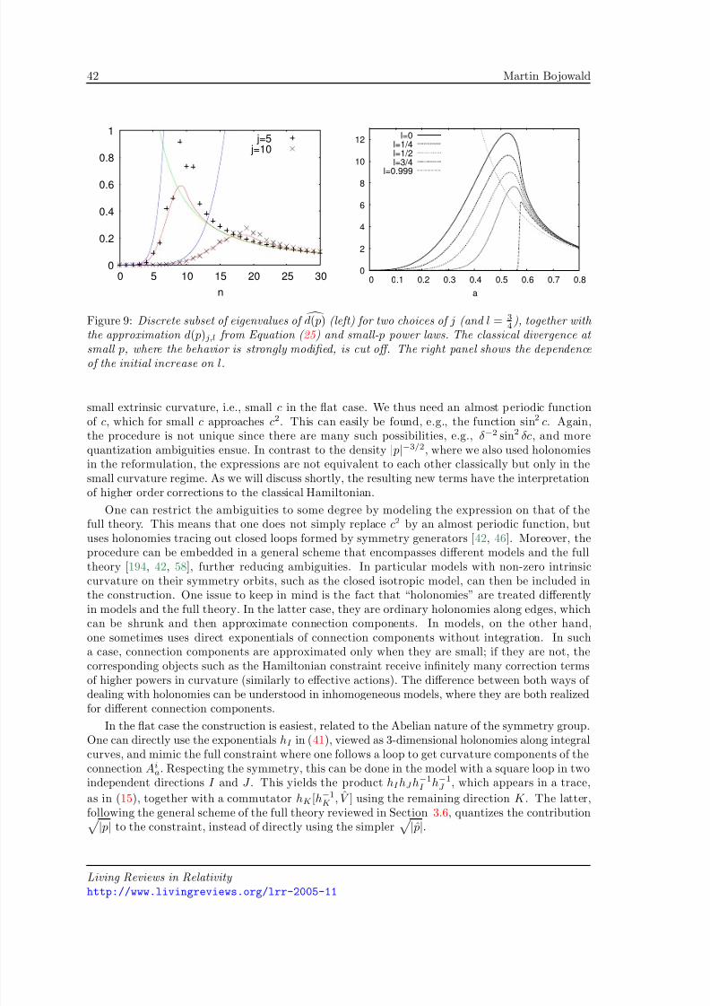
8/3/2019 Martin Bojowald- Loop Quantum Cosmology
http://slidepdf.com/reader/full/martin-bojowald-loop-quantum-cosmology 42/99
42 Martin Bojowald
0
0.2
0.4
0.6
0.8
1
0 5 10 15 20 25 30
n
j=5 j=10
0
2
4
6
8
10
12
0 0.1 0.2 0.3 0.4 0.5 0.6 0.7 0.8
a
l=0l=1/4l=1/2l=3/4
l=0.999
Figure 9: Discrete subset of eigenvalues of
d( p) (left) for two choices of j (and l = 3
4), together with
the approximation d( p)j,l from Equation ( 25 ) and small- p power laws. The classical divergence at
small p, where the behavior is strongly modified, is cut off. The right panel shows the dependenceof the initial increase on l.
small extrinsic curvature, i.e., small c in the flat case. We thus need an almost periodic functionof c, which for small c approaches c2. This can easily be found, e.g., the function sin2 c. Again,the procedure is not unique since there are many such possibilities, e.g., δ−2 sin2 δc, and morequantization ambiguities ensue. In contrast to the density | p|−3/2, where we also used holonomiesin the reformulation, the expressions are not equivalent to each other classically but only in thesmall curvature regime. As we will discuss shortly, the resulting new terms have the interpretationof higher order corrections to the classical Hamiltonian.
One can restrict the ambiguities to some degree by modeling the expression on that of the
full theory. This means that one does not simply replace c2
by an almost periodic function, butuses holonomies tracing out closed loops formed by symmetry generators [42, 46]. Moreover, theprocedure can be embedded in a general scheme that encompasses different models and the fulltheory [194, 42, 58], further reducing ambiguities. In particular models with non-zero intrinsiccurvature on their symmetry orbits, such as the closed isotropic model, can then be included inthe construction. One issue to keep in mind is the fact that “holonomies” are treated differentlyin models and the full theory. In the latter case, they are ordinary holonomies along edges, whichcan be shrunk and then approximate connection components. In models, on the other hand,one sometimes uses direct exponentials of connection components without integration. In sucha case, connection components are approximated only when they are small; if they are not, thecorresponding objects such as the Hamiltonian constraint receive infinitely many correction termsof higher powers in curvature (similarly to effective actions). The difference between both ways of dealing with holonomies can be understood in inhomogeneous models, where they are both realized
for different connection components.
In the flat case the construction is easiest, related to the Abelian nature of the symmetry group.One can directly use the exponentials hI in (41), viewed as 3-dimensional holonomies along integralcurves, and mimic the full constraint where one follows a loop to get curvature components of theconnection Ai
a. Respecting the symmetry, this can be done in the model with a square loop in twoindependent directions I and J . This yields the product hI hJ h
−1I h−1
J , which appears in a trace,
as in (15), together with a commutator hK [h−1K , V ] using the remaining direction K . The latter,
following the general scheme of the full theory reviewed in Section 3.6, quantizes the contribution | p| to the constraint, instead of directly using the simpler
|ˆ p|.
Living Reviews in Relativity http://www.livingreviews.org/lrr-2005-11
8/3/2019 Martin Bojowald- Loop Quantum Cosmology
http://slidepdf.com/reader/full/martin-bojowald-loop-quantum-cosmology 43/99
Loop Quantum Cosmology 43
Taking the trace one obtains a diagonal operator
sin( 12 δc)V cos(1
2 δc) − cos(12 δc)V sin( 1
2 δc)
in terms of the volume operator, as well as the multiplication operator
sin2( 12
δc)cos2( 12
δc) = sin2(δc).
In the triad representation where instead of working with functions c|ψ = ψ(c) one works withthe coefficients ψµ in an expansion |ψ =
µ ψµ|µ, this operator is the square of a difference
operator. The constraint equation thus takes the form of a difference equation [46, 77, 15]
(V µ+5δ − V µ+3δ)eikψµ+4δ(φ) − (2 + k2γ 2δ2)(V µ+δ − V µ−δ)ψµ(φ)
+ (V µ−3δ − V µ−5δ)e−ikψµ−4δ(φ) = −16π
3Gγ 3δ32
PH matter(µ)ψµ(φ) (49)
for the wave function ψµ, which can be viewed as an evolution equation in internal time µ. (Notethat this equation is not valid for k =
−1 since the derivation via a Hamiltonian formulation is
not available in this case.) Thus, discrete spatial geometry implies a discrete internal time [43].The equation above results in the most direct way from a non-symmetric constraint operator withgravitational part acting as
H |µ =3
16πGγ 3δ32P
(V µ+δ − V µ−δ)(e−ik|µ + 4δ − (2 + k2γ 2δ2)|µ + eik|µ − 4δ).
One can symmetrize this operator and obtain a difference equation with different coefficients, whichwe do here after multiplying the operator with sgn p for reasons that will be discussed in the contextof singularities in Section 5.15. The resulting difference equation is
(|∆δV |(µ + 4δ) + |∆δV |(µ))eikψµ+4δ(φ) − 2(2 + k2γ 2δ2)|∆δV |(µ)ψµ(φ)
+ (
|∆δV
|(µ
−4δ) +
|∆δV
|(µ))e−ikψµ
−4δ(φ) =
−32π
3
Gγ 3δ32PH matter(µ)ψµ(φ) (50)
where |∆δV |(µ) := sgn(µ)(V µ+δ − V µ−δ) = |V µ+δ − V µ−δ|.Since sin c|µ = − 1
2 i(|µ+2−|µ−2), the difference equation is of higher order, even formulatedon an uncountable set, and thus has many independent solutions. Most of them, however, oscillateon small scales, i.e., between µ and µ + mδ with small integer m. Others oscillate only on largerscales and can be viewed as approximating continuum solutions. The behavior of all the solutionsleads to possibilities for selection criteria of different versions of the constraint since there arequantization choices. Most importantly, one chooses the routing of edges to construct the squareholonomy, again the spin of a representation to take the trace [116, 201], and factor ordering choicesbetween quantizations of c2 and
| p|. All these choices also appear in the full theory such that
one can draw conclusions for preferred cases there.When the symmetry group is not Abelian and there is non-zero intrinsic curvature, the con-
struction is more complicated. For non-Abelian symmetry groups integral curves as before donot form a closed loop and one needs a correction term related to intrinsic curvature components[46, 62]. Moreover, the classical regime is not as straightforward to specify since connection compo-nents are not necessarily small when there is intrinsic curvature. A general scheme encompassingintrinsic curvature, other symmetric models and the full theory will be discussed in Section 5.14.
5.5 Semiclassical limit and correction terms
When replacing c2 by holonomies we have modified the constraint as a function on the classicalphase space. This is necessary since otherwise the function cannot be quantized, but is different
Living Reviews in Relativity http://www.livingreviews.org/lrr-2005-11
8/3/2019 Martin Bojowald- Loop Quantum Cosmology
http://slidepdf.com/reader/full/martin-bojowald-loop-quantum-cosmology 44/99
44 Martin Bojowald
from the quantization of densities because now the replacements are not equivalent to the originalconstraint classically. Also the limit limδ→0 δ−2 sin2 δc, which would give the classical result, doesnot exist at the operator level.
This situation is different from the full theory, again related to the presence of a partial back-ground [15]. There, the parameter length of edges used to construct appropriate loops is irrelevantand thus can shrink to zero. In the model, however, changing the edge length with respect tothe background does change the operator and the limit does not exist. Intuitively, this can beunderstood as follows: The full constraint operator (15) is a vertex sum obtained after introducinga discretization of space used to choose loops αIJ . This classical regularization sums over all tetra-hedra in the discretization, whose number diverges in the limit where the discretization size shrinksto zero. In the quantization, however, almost all these contributions vanish since a tetrahedronmust contain a vertex of a state in order to contribute non-trivially. The result is independent of the discretization size once it is fine enough, and the limit can thus be taken trivially.
In a homogeneous model, on the other hand, contributions from different tetrahedra of thetriangulation must be identical owing to homogeneity. The coordinate size of tetrahedra drops outof the construction in the full background independent quantization, as emphasized in Section 3.6,
which is part of the reason for the discretization independence. In a homogeneous configurationthe number of contributions thus increases in the limit, but their size does not change. This resultsin an ill-defined limit as we have already seen within the model itself.
The difference between models and the full theory is thus only a consequence of the symmetryand not of different approaches. This will also become clear later in inhomogeneous models whereone obtains a mixture between the two situations. Moreover, in the full theory one has a situationsimilar to symmetric models if one does not only look at the operator limit when the regularizationis removed but also checks the classical limit on semiclassical states. In homogeneous models, theexpression in terms of holonomies implies corrections to the classical constraint when curvaturebecomes larger. This is in analogy to other quantum field theories where effective actions generallyhave higher curvature terms. In the full theory, those correction terms can be seen when one com-putes expectation values of the Hamiltonian constraint in semiclassical states peaked at classical
configurations for the connection and triad. When this classical configuration becomes small involume or large in curvature, correction terms to the classical constraint arise. In this case, thesemiclassical state provides the background with respect to which these corrections appear. Ina homogeneous model, the symmetry already provides a partial background such that correctionterms can be noticed already for the constraint operator itself.
5.5.1 WKB approximation
There are different procedures to make contact between the difference equation and classical con-straints. The most straightforward way is to expand the difference operators in a Taylor series,assuming that the wave function is sufficiently smooth. On large scales, this indeed results in theWheeler–DeWitt equation as a continuum limit in a particular ordering [44]. From then on, onecan use the WKB approximation or Wigner functions as usually.
That this is possible may be surprising because as just discussed the continuum limit δ → 0does not exist for the constraint operator. And indeed, the limit of the constraint equation, i.e., theoperator applied to a wave function, does not exist in general. Even for a wave function the limitδ → 0 does not exist in general since some solutions are sensitive to the discreteness and do nothave a continuum limit at all. When performing the Taylor expansion we already assumed certainproperties of the wave function such that the continuum limit does exist. This then reduces thenumber of independent wave functions to that present in the Wheeler–DeWitt framework, subjectto the Wheeler–DeWitt equation. That this is possible demonstrates that the constraint in termsof holonomies does not have problems with the classical limit.
Living Reviews in Relativity http://www.livingreviews.org/lrr-2005-11
8/3/2019 Martin Bojowald- Loop Quantum Cosmology
http://slidepdf.com/reader/full/martin-bojowald-loop-quantum-cosmology 45/99
Loop Quantum Cosmology 45
The Wheeler–DeWitt equation results at leading order, and in addition higher order termsarise in an expansion of difference operators in terms of δ or γ . Similarly, after the WKB or othersemiclassical approximation there are correction terms to the classical constraint in terms of γ aswell as [99].
This procedure is intuitive, but it is not suitable for inhomogeneous models where the Wheeler–DeWitt representation becomes ill-defined. One can evade this by performing the continuum andsemiclassical limit together. This again leads to corrections in terms of γ as well as , which aremainly of the following form [29]: Matter Hamiltonians receive corrections through the modifieddensity d( p), and there are similar terms in the gravitational part containing
| p|. These are
purely from triad coefficients, and similarly connection components lead to higher order correctionsas well as additional contributions summarized in a quantum geometry potential. A possibleinterpretation of this potential in analogy to the Casimir effect has been put forward in [128]. Arelated procedure to extract semiclassical properties from the difference operator, based on theBohmian interpretation of quantum mechanics, has been discussed in [185].
5.5.2 Effective formulationIn general, one does not only expect higher order corrections for a gravitational action but alsohigher derivative terms. The situation is then qualitatively different since not only correction termsto a given equation arise, but also new degrees of freedom coming from higher derivatives beingindependent of lower ones. In a WKB approximation, this could be introduced by parameterizingthe amplitude of the wave function in a suitable way, but it has not been worked out yet. Analternative approach makes use of a geometrical formulation of quantum mechanics [26], whichnot only provides a geometrical picture of the classical limit but also a clear-cut procedure forcomputing effective Hamiltonians in analogy to effective actions [73].
Instead of using linear operators on a Hilbert space, one can formulate quantum mechanics onan infinite-dimensional phase space. This space is directly obtained from the Hilbert space wherethe inner product defines a metric as well as a symplectic form on its linear vector space (which in
this way even becomes Kahler). This formulation brings quantum mechanics conceptually muchcloser to classical physics, which also facilitates a comparison in a semiclassical analysis.
We thus obtain a quantum phase space with infinitely many degrees of freedom, together witha flow defined by the Schrodinger equation. Operators become functions on this phase spacethrough expectation values. Coordinates can be chosen by suitable parameterizations of a generalwave function, in particular using the expectation values q = q and p = ˆ p together withuncertainties and higher moments. The projection π : H → R2, ψ → (ψ|q|ψ, ψ|ˆ p|ψ) defines thequantum phase space as a fiber bundle over the classical phase space with infinite-dimensionalfibers. Sections of this bundle can be defined by embedding the classical phase space into thequantum phase space by means of suitable semiclassical states.
For a harmonic oscillator this embedding can be done by coherent states which are preserved bythe quantum evolution. This means that the quantum flow is tangential to the embedding of theclassical phase space such that it agrees with the classical flow. The harmonic oscillator thus doesnot receive quantum corrections as is well known from effective actions for free field theories. Othersystems, however, behave in a more complicated manner where in general states spread. This meansthat additional coordinates of the quantum phase space are dynamical and may become excited. If this is the case, the quantum flow differs from the classical flow and an effective Hamiltonian ariseswith correction terms that can be computed systematically. This effective Hamiltonian is given bythe expectation value H in approximate coherent states [16, 206, 188]. In these calculations, onecan include higher degrees of freedom along the fibers, which, through the effective equations of motion, can be related to higher derivatives or higher curvature in the case of gravity.
For a constrained system, such as gravity, one has to compute the expectation value of the
Living Reviews in Relativity http://www.livingreviews.org/lrr-2005-11
8/3/2019 Martin Bojowald- Loop Quantum Cosmology
http://slidepdf.com/reader/full/martin-bojowald-loop-quantum-cosmology 46/99
46 Martin Bojowald
Hamiltonian constraint, i.e., first go to the classical picture and then solve equations of motion.Otherwise, there would simply be no effective equations left after the constraints would alreadyhave been solved. This is the same procedure as in standard effective actions, which one canalso formulate in a constrained manner if one chooses to parameterize time. Indeed, also fornon-constrained systems agreement between the geometrical way to derive effective equations andstandard path integral methods has been shown for perturbations around a harmonic oscillator[73].
5.6 Homogeneity
A Hamiltonian formulation is available for all homogeneous models of Bianchi class A [111], whichhave structure constants C I JK fulfilling C I JI = 0. The structure constants also determine left-
invariant 1-forms ωI in terms of which one can write a homogeneous connection as Aia = φiI ω
I a (see
Appendix B.1) where all freedom is contained in the x-independent φiI . A homogeneous densitized
triad can be written in a dual form with coefficients ˜ pI i conjugate to φiI . As in isotropic models,one absorbs powers of the coordinate volume to obtain variables φiI and pI i .
The kinematics is the same for all class A models, except possibly for slight differences in thediffeomorphism constraint [25, 36]. Connection components define a distinguished triple of su(2)elements φiI τ i, one for each independent direction of space. Holonomies in those directions are then
obtained as h(µI)I = exp(µI φ
iI τ i) ∈ SU(2) with parameters µI for the edge lengths. Cylindrical func-
tions depend on those holonomies, i.e., are countable superpositions of terms f (h(µ1)1 , h(µ2)
2 , h(µ3)3 ).
A basis can be written down as spin network states
f (h(µ1)1 , h
(µ2)2 , h
(µ3)3 ) = ρj1(h
(µ1)1 )A1
B1ρj2(h
(µ2)2 )A2
B2ρj3(h
(µ3)3 )A3
B3K B1B2B3
A1A2A3
where the matrix K specifies how the representation matrices are contracted to a gauge invariantfunction of φiI . There are uncountably many such states for different µI and thus the Hilbert spaceis non-separable. In contrast to isotropic models, the general homogeneous theory is genuinely
SU(2) and therefore not much simpler than the full theory for individual calculations.As a consequence of homogeneity we observe the same degeneracy as in isotropic models where
both spin and edge length appear similarly as parameters. Spins are important to specify thecontraction K and thus appear, e.g., in the volume spectrum. For this one needs to know thespins, and it is not sufficient to consider only products jI δI . On the other hand, there is stilla degeneracy of spin and edge length and keeping both jI and δI independent leaves too manyparameters. It is therefore more difficult to determine what the analog of the Bohr compactificationis in this case.
5.7 Diagonalization
The situation simplifies if one considers diagonal models, which is usually also done in classical
considerations since it does not lead to much loss of information. In a metric formulation, onerequires the metric and its time derivative to be diagonal, which is equivalent to a homogeneousdensitized triad pI i = p(I )ΛI
i and connection φiI = c(I )ΛiI with real numbers cI and pI (where
coordinate volume has been absorbed as described in Appendix B.1) which are conjugate to eachother, cI , pJ = 8πγGδJ I , and internal directions Λi
I as in isotropic models [48]. In fact, thekinematics becomes similar to isotropic models, except that there are now three independentcopies. The reason for the simplification is that we are able to separate off the gauge degreesof freedom in Λi
I from gauge invariant variables cI and pI (except for remaining discrete gaugetransformations changing the signs of two of the pI and cI together). In a general homogenousconnection, gauge-dependent and gauge-invariant parameters are mixed together in φiI , which both
Living Reviews in Relativity http://www.livingreviews.org/lrr-2005-11
8/3/2019 Martin Bojowald- Loop Quantum Cosmology
http://slidepdf.com/reader/full/martin-bojowald-loop-quantum-cosmology 47/99
Loop Quantum Cosmology 47
react differently to a change in µI . This makes it more difficult to discuss the structure of relevantfunction spaces without assuming diagonalization.
As mentioned, the variables pI and cI are not completely gauge invariant since a gauge trans-formation can flip the sign of two components pI and cI while keeping the third fixed. There isthus a discrete gauge group left, and only the total sign sgn( p1 p2 p3) is gauge invariant in additionto the absolute values.
Quantization can now proceed simply by using as Hilbert space the triple product of theisotropic Hilbert space, given by square integrable functions on the Bohr compactification of thereal line. This results in states |ψ =
µ1,µ2,µ3
ψµ1,µ2,µ3 |µ1, µ2, µ3 expanded in an orthonormalbasis
c1, c2, c3|µ1, µ2, µ3 = ei(µ1c1+µ2c2+µ3c3)/2.
Gauge invariance under discrete gauge transformations requires ψµ1,µ2,µ3 to be symmetric undera flip of two signs in µI . Without loss of generality one can thus assume that ψ is defined for allreal µ3 but only non-negative µ1 and µ2.
Densitized triad components are quantized by
ˆ pI |µ1, µ2, µ3 = 12
µI γ2P|µ1, µ2, µ3,
which directly give the volume operator V = |ˆ p1 ˆ p2 ˆ p3| with spectrum
V µ1,µ2,µ3 = ( 12
γ2P)3/2
|µ1µ2µ3|.
Moreover, after dividing out the remaining discrete gauge freedom the only independent sign intriad components is given by the orientation sgn(ˆ p1 ˆ p2 ˆ p3), which again leads to a doubling of themetric minisuperspace with a degenerate subset in the interior, where one of the pI vanishes.
5.8 Homogeneity: Dynamics
The Hamiltonian constraint can be constructed in the standard manner and its matrix elementscan be computed explicitly thanks to the simple volume spectrum. There are holonomy operatorsfor all three directions, and so in the triad representation the constraint equation becomes a partialdifference equation for ψµ1,µ2,µ3 in three independent variables. Its (lengthy) form can be foundin [48] for the Bianchi I model and in [62] for all other class A models.
Simpler cases arise in so-called locally rotationally symmetric (LRS) models, where a non-trivialisotropy subgroup is assumed. Here, only two independent parameters µ and ν remain, where onlyone, e.g., ν can take both signs if discrete gauge freedom is fixed, and the vacuum differenceequation is, e.g., for Bianchi I,
2δ
|ν + 2δ|(ψµ+2δ,ν+2δ − ψµ−2δ,ν+2δ)
+ 12
(
|ν + δ| −
|ν − δ|) ((µ + 4δ)ψµ+4δ,ν − 2µψµ,ν + (µ − 4δ)ψµ−4δ,ν)
−2δ |ν − 2δ|(ψµ+2δ,ν−2δ − ψµ−2δ,ν−2δ)= 0 (51)
from the non-symmetric constraint and
2δ(
|ν + 2δ| +
|ν |)(ψµ+2δ,ν+2δ − ψµ−2δ,ν+2δ)
+(
|ν + δ| −
|ν − δ|) ((µ + 2δ)ψµ+2δ,ν − µψµ,ν + (µ − 2δ)ψµ−2δ,ν)
−2δ(
|ν − 2δ| +
|ν |)(ψµ+2δ,ν−2δ − ψµ−2δ,ν−2δ)
= 0 (52)
Living Reviews in Relativity http://www.livingreviews.org/lrr-2005-11
8/3/2019 Martin Bojowald- Loop Quantum Cosmology
http://slidepdf.com/reader/full/martin-bojowald-loop-quantum-cosmology 48/99
48 Martin Bojowald
from the symmetric version (see also [14]). This leads to a reduction between fully anisotropic andisotropic models with only two independent variables, and provides a class of interesting systemsto analyze effects of anisotropies.
5.9 Inhomogeneous models
Homogeneous models provide a rich generalization of isotropic ones, but inhomogeneities lead tostronger qualitative differences. To start with, at least at the kinematical level one has infinitelymany degrees of freedom and is thus always dealing with field theories. Studying field theoreticalimplications does not require going immediately to the full theory since there are many inhomo-geneous models of physical interest.
We will describe some 1-dimensional models with one inhomogeneous coordinate x and twoothers parameterizing symmetry orbits. A general connection is then of the form (with coordinatedifferentials ωy and ωz depending on the symmetry)
A = Ax(x)Λx(x) dx + Ay(x)Λy(x)ωy + Az(x)Λz(x)ωz + field independent terms (53)
with three real functions AI (x) and three internal directions ΛI (x) normalized to tr(Λ2I ) = −
1
2 ,which in general are independent of each other. The situation in a given point x is thus similarto general homogeneous models with nine free parameters. Correspondingly, there are not manysimplifications from this general form, and one needs analogs of the diagonalization employed forhomogeneous models. What is required mathematically for simplifications to occur is a connectionwith internally perpendicular components, i.e., tr(ΛI ΛJ ) = −1
2δIJ in each point. This arises in
different physical situations.
5.10 Einstein–Rosen waves
One class of 1-dimensional models is given by cylindrically symmetric gravitational waves, withconnections and triads
A = Ax(x)τ 3 dx + (A1(x)τ 1 + A2(x)τ 2) dz + (A3(x)τ 1 + A4(x)τ 2) dϕ, (54)E = E x(x)τ 3
∂
∂x+ (E 1(x)τ 1 + E 2(x)τ 2)
∂
∂z+ (E 3(x)τ 1 + E 4(x)τ 2)
∂
∂ϕ(55)
in cylindrical coordinates. This form is more special than (53), but still not simple enough forarbitrary A1, A2, A3 and A4. Einstein–Rosen waves [109, 34] are a special example of cylindricalwaves subject to the polarization condition A2A4 + A1A3 = 0, and analogously for triad compo-nents. This is just what is needed to restrict the model to internally perpendicular connectioncomponents and is thus analogous to diagonalization in a homogeneous model.
5.10.1 Canonical variables
A difference to homogeneous models, however, is that the internal directions of a connection anda triad do not need to be identical, which in homogeneous models with internal directions Λi
I
is
the case as a consequence of the Gauss constraint ijkφjI pI k = 0. With inhomogeneous fields, now,
the Gauss constraint reads
E x + A1E 2 − A2E 1 + A3E 4 − A4E 3 = 0 (56)
or, after splitting off norms and internal directions
Az :=
A21 + A2
2 , Aϕ :=
A23 + A2
4 (57)
ΛAz :=
A1τ 1 + A2τ 2Az
, ΛAϕ :=
A3τ 1 + A4τ 2Aϕ
(58)
Living Reviews in Relativity http://www.livingreviews.org/lrr-2005-11
8/3/2019 Martin Bojowald- Loop Quantum Cosmology
http://slidepdf.com/reader/full/martin-bojowald-loop-quantum-cosmology 49/99
Loop Quantum Cosmology 49
and analogously E z, E ϕ, ΛzE and Λϕ
E ,
E x + (AzE z + AϕE ϕ)sin α = 0 (59)
with sin α := −2tr(ΛAz Λ
zEτ 3). If E
x
is not constant, α cannot be zero and thus connections andtriads have different internal directions.
As a consequence, E z is not conjugate to Az, anymore, and instead the momentum of Az
is E z cos α [52]. This seems to make a quantization more complicated since the momenta willbe quantized to simple flux operators, but do not directly determine the geometry such as thevolume V = 4π
dx
|E xE zE ϕ|. For this, one would need to know the angle α which depends onboth connections and triads. Moreover, it would not be obvious how to obtain a discrete volumespectrum since then volume does not depend only on fluxes.
It turns out that there is a simple canonical transformation, which allows one to work withcanonical variables E z and E ϕ playing the role of momenta of Az cos α and Aϕ cos α [75]. Thisseems to be undesirable, too, since now the connection variables are modified which play animportant role for holonomies. That these canonical variables are very natural, however, followsafter one considers the structure of spin connections and extrinsic curvature tensors in this model.The new canonical variables are then simply given by Az cos α = γK z, Aϕ cos α = γK ϕ, i.e.,proportional to extrinsic curvature components. Thus, in the inhomogeneous model we simplyreplace connection components with extrinsic curvature in homogeneous directions (note that Ax
remains unchanged) while momenta remain elementary triad components. This is part of a broaderscheme which is also important for the Hamiltonian constraint operator (Section 5.14).
5.10.2 Representation
With the polarization condition the kinematics of the quantum theory simplifies. Relevant holonomiesare given by he(A) = exp( 1
2i ∫ e Ax(x)dx) along edges in the 1-dimensional manifold and
hzv(A) = exp(iγν vK z(v)), hϕv (A) = exp(iγµvK ϕ(v))
in vertices v with real µv, ν v ≥ 0. Cylindrical functions depend on finitely many of those holonomies,whose edges and vertices form a graph in the 1-dimensional manifold. Flux operators, i.e., quan-tized triad components, act simply by
E x(x)T g,k,µ =γ2
P
8π
ke+(x) + ke−(x)
2T g,k,µ (60)
I E zT g,k,µ =
γ2P
4π
v∈I
ν vT g,k,µ (61) I
E ϕT g,k,µ =γ2
P
4π
v∈I
µvT g,k,µ (62)
on a spin network state
T g,k,µ(A) =e∈g
ρke(he)
v∈V (g)
ρµv(γK ϕ(v))ρνv(γK z(v))ρkv(β (v))
=e∈g
exp
12 ike ∫
eAx(x)dx
v∈V (g)
eiγµvKϕ(v)eiγνvKz(v)eikvβ(v), (63)
which also depend on the gauge angle β determining the internal direction of ΛEz . If we solve
the Gauss constraint at the quantum level, the labels kv will be such that a gauge invariant spinnetwork only depends on the gauge invariant combination Ax + β .
Living Reviews in Relativity http://www.livingreviews.org/lrr-2005-11
8/3/2019 Martin Bojowald- Loop Quantum Cosmology
http://slidepdf.com/reader/full/martin-bojowald-loop-quantum-cosmology 50/99
50 Martin Bojowald
Since triad components have simple quantizations, one can directly combine them to get thevolume operator and its spectrum
V k,µ,ν =
γ 3/23P
4√π v µvν v|ke+(v) + ke−(v)|. (64)
The labels µv and ν v are always non-negative, and the local orientation is given through the signof edge labels ke.
Commutators between holonomies and the volume operator will technically be similar to homo-geneous models, except that there are more possibilities to combine different edges. Accordingly,one can easily compute all matrix elements of composite operators such as the Hamiltonian con-straint. The result is only more cumbersome because there are more terms to keep track of. Againas in diagonal homogeneous cases, the triad representation exists and one can formulate the con-straint equation there. Now, however, one has infinitely many coupled difference equations for thewave function since the lapse function is inhomogeneous (one obtains one difference equation foreach vertex).
There are obvious differences to cases considered previously owing to inhomogeneity. For in-stance, each edge label can take positive or negative values, or go through zero during evolutioncorresponding to the fact that a spatial slice does not need to intersect the classical singularityeverywhere. Also the structure of coefficients of the difference equations, though qualitativelysimilar to homogeneous models, is changed crucially in inhomogeneous models, mainly due to thevolume eigenvalues (64). Now, ke+ , say, and thus E x can be zero without volume eigenvalues inneighboring vertices having zero volume.
5.11 Spherical symmetry
For spherically symmetric models, a connection has the form (Appendix B.3)
A = Ax(x)τ 3 dr + (A1(x)τ 1 + A2(x)τ 2) dϑ + (A1(x)τ 2 − A2(x)τ 1)sin ϑ dϕ + τ 3 cos ϑ dϕ (65)
whose field-dependent terms automatically have perpendicular internal directions. In this case, itis not diagonalization as in the polarization condition for Einstein–Rosen waves but a non-trivialisotropy subgroup which leads to this property. The kinematical quantization is then simplified asdiscussed before, with the only difference being that there is only one type of vertex holonomy
hv(A) = exp(iγµvK ϕ(v))
as a consequence of a non-trivial isotropy subgroup. The Hamiltonian constraint can again becomputed explicitly [75].
Spherically symmetric models are usually used for applications to non-rotating black holes, butthey can also be useful for cosmological purposes. They are particularly interesting as models for
the evolution of inhomogeneities as perturbations, which can be applied to gravitational collapsebut also cosmology. In such a context one often reduces the spherically symmetric configurationeven further by requiring a spatial metric
ds2 = qxx(x, t) dx2 + qϕϕ(x, t) dΩ2,
where qxx is related to qϕϕ by ∂ x√
qxx =√
qϕϕ. One example for such a metric is the spatial partof a flat Friedmann–Robertson–Walker space-time, where qϕϕ(x, t) = x2a(t)2. This allows one tostudy perturbations around a homogeneous space-time, which can also be done at the quantumlevel.
Living Reviews in Relativity http://www.livingreviews.org/lrr-2005-11
8/3/2019 Martin Bojowald- Loop Quantum Cosmology
http://slidepdf.com/reader/full/martin-bojowald-loop-quantum-cosmology 51/99
Loop Quantum Cosmology 51
5.12 Loop inspired quantum cosmology
The constructions described so far in this section follow all the steps in the full theory as closelyas possible. Most importantly, one obtains quantum representations inequivalent to those used
in a Wheeler–DeWitt quantization, which results in many further implications. This has inspiredinvestigations where not all the steps of loop quantum gravity are followed, but only the same typeof representation, i.e., the Bohr Hilbert space in an isotropic model, is used. Other constructions,based on ADM rather than Ashtekar variables, are then done in the most straightforward wayrather than a way suggested by the full theory [131].
In isotropic models the results are similar, but already here one can see conceptual differences.Since the model is based on ADM variables, in particular using the metric and not triads, it isnot clear what the additional sign factor sgn(µ), which is then introduced by hand, means geo-metrically. In loop quantum cosmology it arose naturally as orientation of triads, even before itsrole in removing the classical singularity, to be discussed in Section 5.15, had been noticed. (Thenecessity of having both signs available is also reinforced independently by kinematical consistencyconsiderations in the full theory [117].) In homogeneous models the situation is even more compli-
cated since sign factors are still introduced by hand, but not all of them are removed by discretegauge transformations as in Section 5.7 (see [158] as opposed to [14]). Those models are useful toilluminate possible effects, but they also demonstrate how new ambiguities, even with conceptualimplications, arise if guidance from a full theory is lost.
In particular the internal time dynamics is more ambiguous in those models and thus notusually considered. There are then only arguments that the singularity could be avoided throughboundedness of relevant operators, but those statements are not generic in anisotropic models[62] or even the full theory [85]. Moreover, even if all curvature quantities could be shown to bebounded, the evolution could still stop (as happens classically where not any singularity is also acurvature singularity).
5.13 Dynamics
Because irrational numbers are always the result of calculations, never the result of direct measurement, might it not be possible in physics to abandon irrational numbersaltogether and work only with the rational numbers? That is certainly possible, but it would be a revolutionary change. . . .
At some future time, when much more is known about space and time and the other magnitudes of physics, we may find that all of them are discrete.
Rudolf Carnap
An Introduction to the Philosophy of Science
So far we have mainly described the kinematical construction of symmetric models in loopquantum gravity up to the point where the Hamiltonian constraint appears. Since many dynamicalissues in different models appear in a similar fashion, we discuss them in this section with a common
background. The main feature is that dynamics is formulated by a difference equation that by itself,compared to the usual appearance of differential equations, implies new properties of evolution.Depending on the model there are different classes, which even within a given model are subjectto quantization choices. Yet, since there is a common construction procedure many characteristicfeatures are very general.
Classically, curvature encodes the dynamics of geometry and does so in quantum gravity, too.On the other hand, quantum geometry is most intuitively understood in eigenstates of geometry,e.g., a triad representation if it exists, in which curvature is unsharp. Anyway, only solutions to theHamiltonian constraint are relevant, which in general are peaked neither on spatial geometry noron extrinsic curvature. The role of curvature thus has a different, less direct meaning in quantum
Living Reviews in Relativity http://www.livingreviews.org/lrr-2005-11
8/3/2019 Martin Bojowald- Loop Quantum Cosmology
http://slidepdf.com/reader/full/martin-bojowald-loop-quantum-cosmology 52/99
52 Martin Bojowald
gravity. Still, it is instructive to quantize classical expressions for curvature in special situations,such as a−2 in isotropy. Since the resulting operator is bounded, it has played an influential roleon the development of statements regarding the fate of classical singularities.
However, one has to keep in mind that isotropy is a very special case, as emphasized before,and already anisotropic models shed quite a different light on curvature quantities. Isotropy isspecial because there is only one classical spatial length scale given by the scale factor a, such thatintrinsic curvature can only be a negative power such as a−2 just for dimensional reasons. Thatthe modification is not obvious by quantization in the model is illustrated by comparing the intrin-sic curvature term ka−2, which remains unmodified and thus unbounded in the purely isotropicquantization, with the term coming from a matter Hamiltonian where the classical divergence of a−3 is cut off.
In an anisotropic model we do have different classical scales and thus dimensionally also termslike a1a−3
2 are possible. It is then not automatic that the quantization is bounded even if a−32 were
to be bounded. As an example for such quantities consider the spatial curvature scalar given byW ( p1, p2, p3)/( p1 p2 p3) with W in (37) through the spin connection components. When quantizedand then reduced to isotropy, one does obtain a cut-off to the intrinsic curvature term ka−2 as
mentioned in Section 4.9, but the anisotropic expression remains unbounded on minisuperspace.The limit to vanishing triad components is direction dependent and the isotropic case picks outa vanishing limit. However, in general this is not the limit taken by the dynamical trajectories.Similarly, in the full theory one can show that inverse volume operators are not bounded even,in contrast to anisotropic models, on states where the volume eigenvalue vanishes [85]. However,this is difficult to interpret since nothing is known about its relevance for dynamics, and even thegeometrical role of spin labels, and thus of the configurations considered, is unclear.
It is then quantum dynamics that is necessary to see what properties are relevant and howdegenerate configurations are approached. This should allow one to check if the classical boundarya finite distance away is removed in quantum gravity. This can only happen if quantum gravityprovides candidates for a region beyond the classical singularity, and means to probe how to evolvethere. The most crucial aim is to prevent incompleteness of space-time solutions or their quantum
replacements. Even if curvature would be finite, by itself it would not be enough since one couldnot tell if the singularity persists as incompleteness. Only a demonstration of continuing evolutioncan ultimately show that singularities are absent.
5.14 Dynamics: General construction
Not all steps in the construction of the full constraint can be taken over immediately to a modelsince symmetry requirements have to be respected. It is thus important to have a more generalconstruction scheme that shows how generic different steps are, and whether or not crucial inputin a given symmetric situation is needed.
We have already observed one such issue, which is the appearance of holonomies but also simpleexponentials of connection components without integration. This is a consequence of differenttransformation properties of different connection components in a reduced context. Componentsalong remaining inhomogeneous directions, such as Ax for Einstein–Rosen waves, play the role of connection components in the model, giving rise to ordinary holonomies. Other components, suchas Az and Aϕ in Einstein–Rosen waves or all components in homogeneous models, transform asscalars and thus only appear in exponentials without integration. In the overall picture, we have thefull theory with only holonomies, homogeneous models with only exponentials, and inhomogeneousmodels in between where both holonomies and exponentials appear.
Another crucial issue is that of intrinsic curvature encoded in the spin connection. In thefull theory, the spin connection does not have any covariant meaning and in fact can locally bemade to vanish. In symmetric models, however, some spin connection components can become
Living Reviews in Relativity http://www.livingreviews.org/lrr-2005-11
8/3/2019 Martin Bojowald- Loop Quantum Cosmology
http://slidepdf.com/reader/full/martin-bojowald-loop-quantum-cosmology 53/99
Loop Quantum Cosmology 53
covariantly well-defined since not all coordinate transformations are allowed within a model. Inisotropic models, for instance, the spin connection is simply given by a constant proportional tothe curvature parameter. Of particular importance is the spin connection when one considerssemiclassical regimes because intrinsic curvature does not need to become small there in contrastto extrinsic curvature. Since the Ashtekar connection mixes the spin connection and extrinsiccurvature, its semiclassical properties can be rather complicated in symmetric models.
The full constraint is based on holonomies around closed loops in order to approximate Ashtekarcurvature components when the loop becomes small in a continuum limit. For homogeneous direc-tions, however, one cannot shrink the loop and instead works with exponentials of the components.One thus approximates the classical components only when arguments of the exponential are small.If these arguments were always connection components, one would not obtain the right semiclas-sical properties because those components can remain large. In models one thus has to base theconstruction for homogeneous directions on extrinsic curvature components, i.e., subtract off thespin connection from the Ashtekar connection. For inhomogeneous directions, on the other hand,this is not possible since one needs a connection in order to define a holonomy.
At first sight this procedure seems rather ad hoc and even goes half a step back to ADM
variables since extrinsic curvature components are used. However, there are several places wherethis procedure turns out to be necessary for a variety of independent reasons. We have alreadyseen in Section 5.10 that inhomogeneous models can lead to a complicated volume operator whenone insists on using all Ashtekar connection components. When one allows for extrinsic curvaturecomponents in the way just described, on the other hand, the volume operator becomes straight-forward. This appeared after performing a canonical transformation, which rests non-trivially onthe form of inhomogeneous spin connections and extrinsic curvature tensors.
Moreover, in addition to the semiclassical limit used above as justification one also has to discusslocal stability of the resulting evolution equation [59]: Since higher order difference equations haveadditional solutions, one must ensure that they do not become dominant in order not to spoil thecontinuum limit. This is satisfied with the above construction, while it is generically violated if one were to use only connection components.
There is thus a common construction scheme available based on holonomies and exponentials.As already discussed, this is responsible for correction terms in a continuum limit, but also givesrise to the constraint equation being a difference equation in a triad representation, whenever itexists. In homogeneous models the structure of the resulting difference equation is clear, but thereare different open possibilities in inhomogeneous models. This is intimately related to the issue of anomalies, which also appears only in inhomogeneous models.
With a fixed choice, one has to solve a set of coupled difference equations for a wave function onsuperspace. The basic question then always is what kind of initial or boundary value problem has tobe used in order to ensure the existence of solutions with suitable properties, e.g., in a semiclassicalregime. Once this is specified one can already discuss the singularity problem since one needs tofind out if initial conditions in one semiclassical regime together with boundary conditions awayfrom classical singularities suffice for a unique solution on all of superspace. A secondary questionis how this equation can be interpreted as evolution equation for the wave function in an internal
time. This is not strictly necessary and can be complicated owing to the problem of time in general.Nevertheless, when available, an evolution interpretation can be helpful for interpretations.
5.15 Singularities
Il n’est rien de plus precieux que le temps, puisque c’est le prix de l’eternite.
(There is nothing more precious than time, for it is the price of eternity.)Louis Bourdaloue
Sermon sur la perte de temps
Living Reviews in Relativity http://www.livingreviews.org/lrr-2005-11
8/3/2019 Martin Bojowald- Loop Quantum Cosmology
http://slidepdf.com/reader/full/martin-bojowald-loop-quantum-cosmology 54/99
54 Martin Bojowald
In the classical situation, we always have trajectories on superspace running into singularsubmanifolds where some or all densitized triad components vanish. In semiclassical regimes onecan think of physical solutions as wave packets following these trajectories in internal time, but atsmaller triad components spreading and deformations from a Gaussian become stronger. Moreover,discreteness becomes essential and properties of difference equations need to be taken into accountin order to see what is happening at the singular submanifolds.
The simplest situation is given by isotropic models where superspace is one dimensional withcoordinate p. Minisuperspace is thus disconnected classically with two sides separated by theclassical singularity at p = 0. At this point, classical energy densities diverge and there is nowell-defined initial value problem to evolve further. (Sometimes, formal extensions of solutionsbeyond a classical singularity exist [122], but they are never unique and unrelated to the solutionpreceding the singularity. This shows that a resolution of singularities has not only to provide a newregion, but also an evolution there uniquely from initial values at one side.) A Wheeler–DeWittquantization would similarly lead to diverging matter Hamiltonian operators and the initial valueproblem for the wave function generically breaks down. In isotropic loop quantum cosmology wehave already seen that the matter Hamiltonian does not have diverging contributions from inverse
metric components even at the classical singularity. Nevertheless, the evolution could break downif highest order coefficients in the difference equation become zero. This indeed happens with thenon-symmetric constraint (49) or (51), but in these cases can be seen not to lead to any problems:some coefficients can become zero such that the wave function at µ = 0 remains undeterminedby initial conditions, but the wave function at the other side of the classical singularity is stilldetermined uniquely. There is no breakdown of evolution, and thus no singularity [39]. As onecan see, this relies on crucial properties of the loop representation with well-defined inverse metriccomponents and a difference rather than differential equation [43].
Also the structure of difference equations is important, depending on some choices. Most im-portant is the factor ordering or symmetrization chosen. As just discussed, the ordering usedearlier leads to non-singular evolution but with the wave function at the classical singularity itself remaining undetermined. In anisotropic models one can symmetrize the constraint and obtain a
difference equation, such as (52), whose leading order coefficients never vanish. Evolution thennever stops and even the wave function at the classical singularity is determined. In the isotropiccase, direct symmetrization would lead to a break-down of evolution, which thus provides an ex-ample for singular quantum evolution and demonstrates the non-triviality of continuing evolution:The leading order coefficient would then be V µ−3δ−V µ−5δ+V µ+δ−V µ−δ, which vanishes if and onlyif µ = 2δ. Thus, in the backward evolution ψ−2δ remains undetermined, just as ψ0 is undeterminedin the non-symmetric ordering. However, now ψ−2δ would be needed to evolve further. Since it isnot determined by initial data, one would need to prescribe this value, or else the evolution stops.There is thus a new region at negative µ, but evolution does not continue uniquely between the twosides. In such a case, even though curvature is bounded, the quantum system would be singular.Similar behavior happens in other orderings such as when triads are ordered to the left. Note thatalso in the full theory one cannot order triads to the left since otherwise the constraint would notbe densely defined [194].
The breakdown of the symmetric ordering in isotropic models is special and related to thefact that all directions degenerate. The breakdown does not happen for a symmetric ordering inanisotropic or even inhomogeneous systems. One can avert it in isotropic cases by multiplying theconstraint with sgn ˆ p before symmetrizing, so that the additional factor of sgn µ leads to non-zerocoefficients as in (50).
This is the general scheme, which also applies in more complicated cases. The prime examplefor the general homogeneous behavior is given by the Kasner evolution of the Bianchi I model.Here, the approach to the singularity is not isotropic but given in such a way that two of thethree diagonal metric components become zero while the third one diverges. This would lead to
Living Reviews in Relativity http://www.livingreviews.org/lrr-2005-11
8/3/2019 Martin Bojowald- Loop Quantum Cosmology
http://slidepdf.com/reader/full/martin-bojowald-loop-quantum-cosmology 55/99
Loop Quantum Cosmology 55
a different picture than described before since the classical singularity then lies at the infiniteboundary of metric or co-triad minisuperspace. Also unlike in the isotropic case, densities orcurvature potentials are not necessarily bounded in general as functions on minisuperspace, andthe classical dynamical approach is important. In densitized triad variables, however, we have asituation as before since here all components approach zero, although at different rates. Now theclassical singularity is in the interior of minisuperspace and one can study the evolution as before,again right through the classical singularity. Note that densitized triad variables were required fora background independent quantization, and now independently for non-singular evolution.
Other homogeneous models are more complicated since for them Kasner motion takes place witha potential given by curvature components. Approximate Kasner epochs arise when the potentialis negligible, intermitted by reflections at the potential walls where the direction of Kasner motionin the anisotropy plane changes. Still, since in each Kasner epoch the densitized triad componentsdecrease, the classical singularity remains in the interior and is penetrated by the discrete quantumevolution.
One can use this for indications as to the general inhomogeneous behavior by making use of the BKL scenario. If this can be justified, in each spatial point the evolution of geometry is given
by a homogeneous model. For the quantum formulation this indicates that also here classicalsingularities are removed. However, it is by no means clear whether the BKL scenario appliesat the quantum level since even classically it is not generally established. If the scenario is notrealized (or if some matter systems can change the local behavior), diverging p are possible and thebehavior would qualitatively be very different. One thus has to study the inhomogeneous quantumevolution directly as done before for homogeneous cases.
In the 1-dimensional models described here classical singularities arise when E x becomes zero.Since this is now a field, it depends on the point x on the spatial manifold where the slice hitsthe classical singularity. At each such place, midisuperspace opens up to a new region not reachedby the classical evolution, where the sign of E x(x) changes and thus the local orientation of thetriad. Again, the kinematics automatically provides us with these new regions just as needed, andquantum evolution continues. Also, the scheme is realized much more non-trivially, and now even
the non-symmetric ordering is not allowed. This is a consequence of the fact that ke = 0 for a singleedge label does not imply that neighboring volume eigenvalues vanish. There is thus no obviousdecoupling in a non-singular manner, and it shows how less symmetric situations put more stringentrestrictions on the allowed dynamics. Still, the availability of other possibilities, maybe with leadingcoefficients which can vanish and result in decoupling, needs to be analyzed. Most importantly, thesymmetric version still leads to non-singular evolution even in those inhomogeneous cases whichhave local gravitational degrees of freedom [57].
There is thus a general scheme for the removal of singularities: In the classical situation, onehas singular boundaries of superspace which cannot be penetrated. Densitized triad variables thenlead to new regions, given by a change in the orientation factor sgn det E which, however, doesnot help classically since singularities remain as interior boundaries. For the quantum situationone has to look at the constraint equation and see whether or not it uniquely allows to continuea wave function to the other side (which does not require time parameters even though they maybe helpful if available). This usually depends on factor ordering and other choices that arise inthe construction of constraint operators and play a role also for the anomaly issue. One can thusfix ambiguities by selecting a non-singular constraint if possible. However, the existence of non-singular versions, as realized in a natural fashion in homogeneous models, is a highly non-trivialand by no means automatic property of the theory showing its overall consistency.
In inhomogeneous models the issue is more complicated. We thus have a situation where thetheory, which so far is well-defined, can be tested by trying to extend results to more generalcases. It should also be noted that different models should not require different quantizationchoices unless symmetry itself is clearly responsible (as happens with the orientation factor in the
Living Reviews in Relativity http://www.livingreviews.org/lrr-2005-11
8/3/2019 Martin Bojowald- Loop Quantum Cosmology
http://slidepdf.com/reader/full/martin-bojowald-loop-quantum-cosmology 56/99
56 Martin Bojowald
symmetric ordering for an isotropic model, or when non-zero spin connection components receivecovariant meaning in models), but that there should rather be a common scheme leading to non-singular behavior. This puts further strong conditions on the construction, and is possible only if one knows how models and the full theory are related.
5.16 Initial/boundary value problems
In isotropic models the gravitational part of the constraint corresponds to an ordinary differenceoperator which can be interpreted as generating evolution in internal time. One thus needs tospecify only initial conditions to solve the equation. The number of conditions is large since, first,the procedure to construct the constraint operator usually results in higher order equations and,second, this equation relates values of a wave function ψµ defined on an uncountable set. In general,one thus has to choose a function on a real interval unless further conditions are used.
This can be achieved, for instance, by using observables that can reduce the kinematical frame-work back to wave functions defined on a countable discrete lattice [202]. Similar restrictions cancome from semiclassical properties or the physical inner product [162], all of which has not yet
been studied in generality.The situation in homogeneous models is similar, but now one has several gravitational degrees
of freedom only one of which is interpreted as internal time. One has a partial difference equationfor a wave function on a minisuperspace with boundary, and initial as well as boundary conditionsare required [48]. Boundary conditions are imposed only at non-singular parts of minisuperspacesuch as µ = 0 in LRS models (51). They must not be imposed at places of classical singularities,of course, where instead the evolution must continue just as at any regular part.
In inhomogeneous models, then, there are not only many independent kinematical variablesbut also many difference equations for only one wave function on midisuperspace. These differenceequations are of a similar type as in homogeneous models, but they are coupled in complicatedways. Since one has several choices in the general construction of the constraint, there are differentpossibilities for the way how difference equations arise and are coupled. Not all of them are expected
to be consistent, i.e., in many cases some of the difference equations will not be compatible suchthat there would be no non-zero solution at all. This is related to the anomaly issue since thecommutation behavior of difference operators is important for properties and the existence of common solutions.
So far, the evolution operator in inhomogeneous models has not been studied in detail, andsolutions in this case remain poorly understood. The difficulty of this issue can be illustrated bythe expectations in spherical symmetry where there is only one classical physical degree of freedom.If this is to be reproduced for semiclassical solutions of the quantum constraint, there must be asubtle elimination of infinitely many kinematical degrees of freedom such that in the end only onephysical degree of freedom remains. Thus, from the many parameters needed in general to specify asolution to a set of difference equations, only one can remain when compatibility relations betweenthe coupled difference equations and semiclassicality conditions are taken into account.
How much this cancellation depends on semiclassicality and asymptotic infinity conditionsremains to be seen. Some influence is to be expected since classical behavior should have a bearingon the correct reproduction of classical degrees of freedom. However, it may also turn out thatthe number of solutions to the quantum constraint is more sensitive to quantum effects. It isalready known from isotropic models that the constraint equation can imply additional conditionsfor solutions beyond the higher order difference equation, as we will discuss in Section 5.18. Thisusually arises at the place of classical singularities where the order of the difference equationcan change. Since the quantum behavior at classical singularities is important here, the numberof solutions can be different from the classically expected freedom, even when combined withpossible semiclassical requirements far away from the singularity. We will now first discuss these
Living Reviews in Relativity http://www.livingreviews.org/lrr-2005-11
8/3/2019 Martin Bojowald- Loop Quantum Cosmology
http://slidepdf.com/reader/full/martin-bojowald-loop-quantum-cosmology 57/99
Loop Quantum Cosmology 57
requirements in semiclassical regimes, followed by more information on possibly arising additionalconditions for solutions.
5.17 Pre-classicality and boundednessThe high order of difference equations implies that there are in general many independent solu-tions, most of which are oscillating on small scales, i.e., when the labels change only slightly. Onepossibility to restrict the number of solutions then is to require suppressed or even absent oscilla-tions on small scales [40]. Intuitively, this seems to be a pre-requisite for semiclassical behavior andhas thus been called pre-classicality. It can be motivated by the fact that a semiclassical solutionshould not be sensitive to small changes of, e.g., the volume by amounts of Planck size. However,even though the criterion sounds intuitively reasonable, there is so far no justification throughmore physical arguments involving observables or measurement processes to extract informationfrom wave functions. The status of pre-classicality as a selection criterion is thus not final.
Moreover, pre-classicality is not always consistent in all disjoint classical regimes or with otherconditions. For instance, as discussed in the following section, there can be additional conditions
on wave functions arising from the constraint equation at the classical singularity. Such conditionsdo not arise in classical regimes, but they nevertheless have implications for the behavior of wavefunctions there through the evolution equation [87, 86]. Pre-classicality also may not be possibleto impose in all disconnected classical regimes. If the evolution equation is locally stable – whichis a basic criterion for constructing the constraint – choosing initial values in classical regimes,which do not have small-scale oscillations, guarantees that oscillations do not build up throughevolution in a classical regime [59]. However, when the solution is extended through the quantumregime around a classical singularity, oscillations do arise and do not in general decay after a newsupposedly classical regime beyond the singularity is entered. It is thus not obvious that indeeda new semiclassical region forms even if the quantum evolution for the wave function is non-singular. On the other hand, evolution does continue to large volume and macroscopic regions,which is different from other scenarios such as [124] where inhomogeneities have been quantized
on a background.A similar issue is the boundedness of solutions, which also is motivated intuitively by referring
to the common probability interpretation of quantum mechanics [119] but must be supportedby an analysis of physical inner products. The issue arises in particular in classically forbiddenregions where one expects exponentially growing and decaying solutions. If a classically forbiddenregion extends to infinite volume, as happens for models of recollapsing universes, the probabilityinterpretation would require that only the exponentially decaying solution is realized. As before,such a condition at large volume is in general not consistent in all asymptotic regions or with otherconditions arising in quantum regimes.
Both issues, pre-classicality and boundedness, seem to be reasonable, but their physical signif-icance has to be founded on properties of the physical inner product. They are rather straight-forward to analyze in isotropic models without matter fields, where one is dealing with ordinarydifference equations. However, other cases can be much more complicated such that conclusionsdrawn from isotropic models alone can be misleading. Moreover, numerical investigations have tobe taken with care since in particular for boundedness an exponentially increasing contributioncan easily arise from numerical errors and dominate the exact, potentially bounded solution.
One thus needs analytical or at least semi-analytical techniques to deal with these issues. Forpre-classicality one can advantageously use generating function techniques [87] if the differenceequation is of a suitable form, e.g., has only coefficients with integer powers of the discrete pa-rameter. The generating function G(x) :=
n ψnxn for a solution ψn on an equidistant lattice
then solves a differential equation equivalent to the difference equation for ψn. If G(x) is known,one can use its pole structure to get hints for the degree of oscillations in ψn. In particular the
Living Reviews in Relativity http://www.livingreviews.org/lrr-2005-11
8/3/2019 Martin Bojowald- Loop Quantum Cosmology
http://slidepdf.com/reader/full/martin-bojowald-loop-quantum-cosmology 58/99
58 Martin Bojowald
behavior around x = −1 is of interest to rule out alternating behavior where ψn is of the formψn = (−1)nξn with ξn > 0 for all n (or at least all n larger than a certain value). At x = −1we then have G(−1) =
n ξn, which is less convergent than the value for a non-alternating so-
lution ψn = ξn resulting in G(−
1) = n
(−
1)nξn. One can similarly find conditions for the polestructure to guarantee boundedness of ψn, but the power of the method depends on the form of the difference equation. More general techniques are available for the boundedness issue, and alsofor alternating behavior, by mapping the difference equation to a continued fraction which canbe evaluated analytically or numerically [71]. One can then systematically find initial values forsolutions that are guaranteed to be bounded.
5.18 Dynamical initial conditions
I am Aton when I am alone in the Nun, but I am Re when he appears, in the moment when he starts to govern what he has created.
Book of the Dead
The traditional subject of quantum cosmology is the imposition of initial conditions for the wavefunction of a universe in order to guarantee its uniqueness. In the Wheeler–DeWitt framework thisis done at the singularity a = 0, sometimes combined with final conditions in the classical regime.One usually uses intuitive pictures as guidance, akin to Lemaitre’s primitive atom whose decay issupposed to have created the world, Tryon’s and Vilenkin’s tunneling event from nothing, or theclosure of space-time into a Euclidean domain by Hartle and Hawking.
In the latter approaches, which have been formulated as initial conditions for solutions of theWheeler–DeWitt equation [204, 121], the singularity is still present at a = 0, but re-interpretedas a meaningful physical event through the conditions. In particular, the wave function is stillsupported at the classical singularity, i.e., ψ(0) = 0, in contrast to DeWitt’s original idea of requiring ψ(0) = 0 as a means to argue for the absence of singularities in quantum gravity [ 104].DeWitt’s initial condition is in fact, though most appealing conceptually, not feasible in general
since it does not lead to a well-posed initial value formulation in more complicated models: theonly solution would then vanish identically. Zeh tried to circumvent this problem, for instanceby proposing an ad hoc Planck potential, which is noticeable only at the Planck scale and makesthe initial problem well-defined [89]. However, the problem remains that in general there is nosatisfying origin of initial values.
In all these ideas, the usual picture in physics has been taken that there are dynamical lawsdescribing the general behavior of a physical system, and independently initial or boundary con-ditions to select a particular situation. This is reasonable since usually one can prepare a system,corresponding to choosing initial and boundary values, and then study its behavior as determinedby the dynamical laws. For cosmology, however, this is not appropriate since there is no way toprepare the universe.
At this point, there is a new possibility opened up by loop quantum cosmology where the dy-namical law and initial conditions can be part of the same entity [ 40, 78, 49]. This is a specialtyof difference equations whose order can change locally, in contrast to differential equations. Math-ematically, such a difference equation would be called singular since its leading order coefficientscan become zero. However, physically we have already seen that the behavior is non-singular sincethe evolution does not break down.
The difference equation follows from the constraint equation, which is the primary object incanonical quantum gravity. As discussed before, it is usually of high order in classical regimes,where the number of solutions can be restricted, e.g., by pre-classicality. But this, at most, bringsus to the number of solutions that we have for the Wheeler–DeWitt equation such that one needsadditional conditions as in this approach. The new aspect now is that this can follow from the
Living Reviews in Relativity http://www.livingreviews.org/lrr-2005-11
8/3/2019 Martin Bojowald- Loop Quantum Cosmology
http://slidepdf.com/reader/full/martin-bojowald-loop-quantum-cosmology 59/99
Loop Quantum Cosmology 59
constraint equation itself: since the order of the difference equation can become smaller at theclassical singularity, there are less solutions than expected from the semiclassical behavior. In thesimplest models, this is just enough to result in a unique solution up to norm, as appropriatefor a wave function describing a universe. In those cases, the dynamical initial conditions arecomparable to DeWitt’s initial condition, albeit in a manner that is well-posed even in some caseswhere DeWitt’s condition is not [64].
In general, the issue is not clear but should be seen as a new option presented by the discreteformulation of loop quantum cosmology. Since there can be many conditions to be imposed onwave functions in different regimes, one has to see in each model whether or not suitable non-zero solutions remain at all. In fact, some first investigations indicate that different requirementstaken together can be very restrictive [86], which seems to relate well with the non-separabilityof the kinematical Hilbert space [98]. So far, only homogeneous models have been investigatedin detail, but the mechanism of decoupling is known not to be realized in an identical manner ininhomogeneous models.
Inhomogeneous models can add qualitatively new ingredients also to the issue of initial con-ditions due to the fact that there are many coupled difference equations. There can then be
consistency conditions for solutions to the combined system which can strongly restrict the num-ber of independent solutions. This may be welcome, e.g., in spherical symmetry where a singlephysical parameter remains, but the restriction can easily become too strong even below the clas-sically expected one. Since the consistency between difference equations is related to the anomalyissue, there may be an important role played by quantum anomalies. While classically anomaliesshould be absent, the quantum situation can be different since it also takes the behavior at theclassical singularity into account and is supposed to describe the whole universe. Anomalies canthen be precisely what one needs in order to have a unique wave function of a universe even in in-homogeneous cases where initially there is much more freedom. This does not mean that anomaliesare simply ignored or taken lightly since it is difficult to arrange having the right balance betweenmany solutions and no non-zero solution at all. However, quantum cosmology suggests that it isworthwhile to have a less restricted, unconventional view on the anomaly issue.
5.19 Summary
There is a general construction of a loop representation in the full theory and its models, whichis characterized by compactified connection spaces and discrete triad operators. Strong simplifica-tions of some technical and conceptual steps occur in diverse models. Such a general constructionallows a view not only on the simplest case, isotropy, but on essentially all representative systemsfor gravity.
Most important is the dynamics, which in the models discussed here can be formulated bya difference equation on superspace. A general scheme for a unique extension of wave functionsthrough classical singularities is realized, such that the quantum theory is non-singular. Thisgeneral argument, which has been verified in many models, is quite powerful since it does not require
detailed knowledge of or assumptions about matter. It is independent of the availability of a globalinternal time, and so the problem of time does not present an obstacle. Moreover, a complicateddiscussion of quantum observables can be avoided since once it is known that a wave function can becontinued uniquely one can extract relational information at both sides of the classical singularity.(If observables would distinguish both sides with their opposite orientations, they would stronglybreak parity even on large scales in contradiction with classical gravity.) Similarly, information onthe physical inner product is not required since there is a general statement for all solutions of theconstraint equation. The uniqueness of an extension through the classical singularity thus remainseven if some solutions have to be excluded for the physical Hilbert space or factored out if theyhave zero norm.
Living Reviews in Relativity http://www.livingreviews.org/lrr-2005-11
8/3/2019 Martin Bojowald- Loop Quantum Cosmology
http://slidepdf.com/reader/full/martin-bojowald-loop-quantum-cosmology 60/99
60 Martin Bojowald
This is far from saying that observables or the physical inner product are irrelevant for anunderstanding of dynamical processes. Such constructions can, fortunately, be avoided for a generalstatement of non-singular evolution in a wide class of models. For details of the transition and toget information of the precise form of space-time at the other side of classical singularities, however,all those objects are necessary and conceptual problems in their context have to be understood.
So far, the transition has often been visualized by intuitive pictures such as a collapsing uni-verse turning its inside out when orientation is reversed. An hourglass presents a picture for theimportance of discrete quantum geometry close to the classical singularity and the emergence of continuous geometry on large scales: Away from the bottleneck of the hourglass, its sand seemsto be sinking down almost continuously. Directly at the bottleneck with its small circumference,however, one can see that time measured by the hourglass proceeds in discrete steps – one grainat a time.
The main remaining issue for the mechanism to remove singularities then is the question howthe models, where it has been demonstrated, are related to the full theory and to what extent theyare characteristic for full quantum geometry.
Living Reviews in Relativity http://www.livingreviews.org/lrr-2005-11
8/3/2019 Martin Bojowald- Loop Quantum Cosmology
http://slidepdf.com/reader/full/martin-bojowald-loop-quantum-cosmology 61/99
Loop Quantum Cosmology 61
6 Models within the Full Theory
If he uses a model at all, he is always aware that it pictures only certain aspects of thesituation and leaves out other aspects. The total system of physics is no longer required to be such that all parts of its structure can be clearly visualized. . . .
A physicist must always guard against taking a visual model as more than a pedagogical device or makeshift help. At the same time, he must also be alert to the possibility that a visual model can, and sometimes does, turn out to be literally accurate. Naturesometimes springs such surprises.
Rudolf Carnap
An Introduction to the Philosophy of Science
In the preceding section, the link between models and the full theory was given through thesame basic variables and the same kind of representation used, as well as a general constructionscheme for the Hamiltonian constraint operator. The desired simplifications were realized thanks
to the symmetry conditions, but not too strongly since basic features of the full theory are stillrecognizable in models. For instance, even though possible in many ways and often made useof, we did not employ special gauges or coordinate or field dependent transformations obscuringthe relation. The models are thus as close to the full theory as possible while making full use of simplifications in order to have explicit applications.
Still, there are always some differences not all of which are easy to disentangle. For instance,we have discussed possible degeneracies between spin labels and edge lengths of holonomies, whichcan arise in the presence of a partial background and lead to new ambiguity parameters not presentin the full theory. The question thus arises what the precise relation between models and the fulltheory is, or even how and to what extent a model for a given symmetry type can be derived fromthe full theory.
This is possible for the basic representation: The symmetry and the partial background it
provides can be used to define natural subalgebras of the full holonomy/flux algebra by usingholonomies and fluxes along symmetry generators and averaging in a suitable manner. Since thefull representation is unique and cyclic, it induces uniquely a representation of models that istaken directly from the full theory. This will now be described independently for states and basicoperators to provide the idea and to demonstrate the role of the extra structure involved. See also[57] and [63] for illustrations in the context of spherical symmetry and anisotropy, respectively.
6.1 Symmetric states
One can imagine to construct states that are invariant under a given action of a symmetry groupon space by starting with a general state and naively summing over all its possible translates byelements of the symmetry group. For instance on spin network states, the symmetry group acts by
moving the graph underlying the spin network, keeping the labels fixed. Since states with differentgraphs are orthogonal to each other, the sum over uncountably many different translates cannot benormalizable. In simple cases, such as for graphs with a single edge along a symmetry generator,one can easily make sense of the sum as a distribution. But this is not clear for arbitrary states,in particular for states whose graphs have vertices, which on the other hand would be neededfor sufficient generality. A further problem is that any such action of a symmetry group is asubgroup of the diffeomorphism group. At least on compact space manifolds where there areno asymptotic conditions for diffeomorphisms in the gauge group, it then seems that any groupaveraged diffeomorphism invariant state would already be symmetric with respect to arbitrarysymmetries, which is obviously not sensible.
Living Reviews in Relativity http://www.livingreviews.org/lrr-2005-11

8/3/2019 Martin Bojowald- Loop Quantum Cosmology
http://slidepdf.com/reader/full/martin-bojowald-loop-quantum-cosmology 62/99
62 Martin Bojowald
In fact, symmetries and (gauge) diffeomorphisms are conceptually very different, even thoughmathematically they are both expressed by group actions on a space manifold. Gauge diffeomor-phisms are generated by first class constraints of the theory, which in canonical quantum gravityare imposed in the Dirac manner [105] or following refined algebraic quantization [28], convenientlydone by group averaging [153]. Symmetries, however, are additional conditions imposed on a giventheory to extract a particular sector of special interest. They can also be formulated as constraintsadded to the theory, but these constraints must be second class for a well defined framework:One obtains a consistent reduced theory, e.g., with a non-degenerate symplectic structure, only if configuration and momentum variables are required to be symmetric in the same (or dual) way.
In the case of gravity in Ashtekar variables, the symmetry type determines, along the lines of Appendix A the form of invariant connections and densitized triads defining the phase space of thereduced model. At the quantum level, however, one cannot keep connections and triads on the samefooting since a polarization is required. One usually uses the connection representation in loopquantum gravity such that states are functionals on the space of connections. In a minisuperspacequantization of the classically reduced model states would then be functionals only of invariantconnections for the given symmetry type. This suggests to define symmetric states in the fulltheory to be those states whose support contains invariant connections as a dense subset [66, 38](one requires only a dense subset because possible generalized connections must be allowed for).As such, they must necessarily be distributional, as already expected from the naive attempt atconstruction. Symmetric states thus form a subset of the distributional space Cyl∗. In this manner,only the reduced degrees of freedom are relevant, i.e., the reduction is complete, and all of themare indeed realized, i.e., the reduction is not too strong. Moreover, an “averaging” map from anon-symmetric state to a symmetric one can easily be defined by restricting the non-symmetricstate to the space of invariant connections and requiring it to vanish everywhere else.
This procedure defines states as functionals, but since there is no inner product on the fullCyl∗ this does not automatically result in a Hilbert space. Appropriately defined subspaces of Cyl∗, nevertheless, often carry natural inner products, which is also the case here. In fact, sincethe reduced space of invariant connections can be treated by the same mathematical techniquesas the full space, it carries an analog of the full Ashtekar–Lewandowski measure and this is indeedinduced from the unique representation of the full theory. The only difference is that in generalan invariant connection is not only determined by a reduced connection but also by scalar fields(see Appendix A). As in the full theory, this space Ainv of reduced connections and scalars iscompactified to the space Ainv of generalized invariant connections on which the reduced Hilbertspace is defined. One thus arrives at the same Hilbert space for the subset of symmetric states inCyl∗ as used before for reduced models, e.g., using the Bohr compactification in isotropic models.The new ingredient now is that these states have meaning in the full theory as distributions, whoseevaluation on normalizable states depends on the symmetry type and partial background structureused.
That the symmetric Hilbert space obtained in this manner is identical to the reduced loopquantization of Section 5 does not happen by definition but is a result of the procedure. Thesupport of a distribution is by definition a closed subset of the configuration space, and wouldthus be larger than just the set of generalized invariant connections if Ainv would not be a closedsubset in A. In such a case, the reduction at the quantum level would give rise to more degreesof freedom than a loop quantization of the classically reduced model. As shown in [66], however,the set of invariant connections is a closed subset of the full space of connections such that loopquantum cosmology can be interpreted as a minisuperspace quantization.
Living Reviews in Relativity http://www.livingreviews.org/lrr-2005-11
8/3/2019 Martin Bojowald- Loop Quantum Cosmology
http://slidepdf.com/reader/full/martin-bojowald-loop-quantum-cosmology 63/99
Loop Quantum Cosmology 63
6.2 Basic operators
In the classical reduction, symmetry conditions are imposed on both connections and triads, butso far at the level of states only connections have been taken into account. Configuration and
momentum variables play different roles in any quantum theory since a polarization is necessary.As we based the construction on the connection representation, symmetric triads have to be imple-mented at the operator level. (There cannot be additional reduction steps at the state level since,as we already observed, states just implement the right number of reduced degrees of freedom.)
Classically, the reduction of phase space functions is simply done by pull back to the reducedphase space. The flow generated by the reduced functions then necessarily stays in the reducedphase space and defines canonical transformations for the model. An analog statement in thecorresponding quantum theory would mean that the reduced state space would be fixed by fulloperators such that their action (or dual action on distributions) could directly be used in themodel without further work. This, however, is not the case with the reduction performed so far.We have considered only connections in the reduction of states, and also classically a reduction toa subspace Ainv × E , where connections are invariant but not triads, would be incomplete. First,
this would not define a phase space of its own with a non-degenerate symplectic structure. Moreimportant in this context is the fact that this subspace would not be preserved by the flow of reduced functions.
As an example (see also [52] for a different discussion in the spherically symmetric model) weconsider a diagonal homogeneous model, such as Bianchi I for simplicity, with connections of theform Ai
adxa = c(I )ΛiI ω
I and look at the flow generated by the full volume V =
d3x
|det E |. Itis straightforward to evaluate the Poisson bracket
Aia(x), V = 2πγGabcijkE bjE ck/
|det E |
already used in (13). A point on Ainv × E characterized by c(I )ΛiI and an arbitrary triad thus
changes infinitesimally by
δ(c(I )ΛiI ) = 2πγGIbcijkE bjE ck/ |det E |,which does not preserve the invariant form: First, on the right hand side we have arbitrary fields E such that δ(c(I )Λi
I ) is not homogeneous. Second, even if we would restrict ourselves to homogeneousE , δ(c(I )Λi
I ) would not be of the original diagonal form. This is the case only if δ(c(I )ΛiI ) =
ΛiI δ(c(I )) since only the cI are canonical variables. The latter condition is satisfied only if
ijkΛjI δ(c(I )Λi
I ) = 4πγGIbcΛj(I )E bi E cj/
|det E |
vanishes, which is not the case in general. This condition is true only if E ai ∝ Λai , i.e., if we restrict
the triads to be of diagonal homogeneous form just as the connections.A reduction of only one part of the canonical variables is thus incomplete and leads to a
situation where most phase space functions generate a flow that does not stay in the reducedspace. Analogously, the dual action of full operators on symmetric distributional states does notin general map this space to itself. Thus, an arbitrary full operator maps a symmetric state to anon-symmetric one and cannot be used to define the reduced operator. In general, one needs asecond reduction step that implements invariant triads at the level of operators by an appropriateprojection of its action back to the symmetric space. This can be quite complicated, and fortunatelythere are special full operators adapted to the symmetry for which this step is not necessary.
From the above example, it is clear that those operators must be linear in the momenta E ai ,for otherwise one would have a triad remaining after evaluating the Poisson bracket, which onAinv × E would not be symmetric everywhere. Fluxes are linear in the momenta, so we can try
Living Reviews in Relativity http://www.livingreviews.org/lrr-2005-11
8/3/2019 Martin Bojowald- Loop Quantum Cosmology
http://slidepdf.com/reader/full/martin-bojowald-loop-quantum-cosmology 64/99
64 Martin Bojowald
pK(z0) := Sz0
d2yΛk(K)E akωK
a where S z0 is a surface in the IJ -plane at position z = z0 in the K -
direction. By choosing a surface along symmetry generators X I and X J this expression is adaptedto the symmetry, even though it is not fully symmetric yet since the position z0 has to be chosen.
Again, we compute the Poisson bracket
Aia(x), pK(z0) = 8πγGΛi
(K)
Sz0
δ(x, y)ωKa (y) d2y
resulting inδ(c(I )Λi
I ) = 8πγGΛiI δ(z, z0).
Also here the right hand side is not homogeneous, but we have ijkΛjI δ(c(I )Λk
I ) = 0 such thatthe diagonal form is preserved. The violation of homogeneity is expected since the flux is nothomogeneous. This can easily be remedied by “averaging” the flux in the K -direction to
pK := limN →∞
N −1N
α=1
pK(αN −1L0),
where L0 is the coordinate length of the K -direction if it is compact. For any finite N theexpression is well-defined and can directly be quantized, and the limit can be performed in awell-defined manner at the quantum level of the full theory.
Most importantly, the resulting operator preserves the form of symmetric states for the diagonalhomogeneous model in its dual action, corresponding to the flux operator of the reduced model asused before. In averaging the full operator the partial background provided by the group actionhas been used, which is responsible for the degeneracy between edge length and spin in one reducedflux label. Similarly, one can obtain holonomy operators along the I -direction that preserve theform of symmetric states after averaging them along the J and K directions (in such a way that theedge length is variable in the averaging limit). Thus, the dual action of full operators is sufficientto derive all basic operators of the model from the full theory. The representation of states and
basic operators, which was seen to be responsible for most effects in loop quantum cosmology, isthus directly linked to the full theory. This, then, defines the cosmological sector of loop quantumgravity.
6.3 Quantization before reduction
When quantizing a model after a classical reduction, there is much freedom even in choosingthe basic representation. For instance, in homogeneous models one can use the Wheeler–DeWittformulation based on the Schrodinger representation of quantum mechanics. In other models onecould choose different smearings, e.g., treating triad components by holonomies and connectioncomponents by fluxes, since transformation properties can change from the reduced point of view(see, e.g., [52]). There is thus no analog of the uniqueness theorem of the full theory, and models
constructed in this manner would have much inherent freedom even at a basic level. With the linkto the full theory, however, properties of the unique representation there are transferred directly tomodels, resulting in analogous properties such as discrete fluxes and an action only of exponentiatedconnection components. This is sufficient for a construction by analogy of composite operators,such as the Hamiltonian constraint according to the general scheme.
If the basic representation is taken from the full quantization, one makes sure that manyconsistency conditions of quantum gravity are already observed. This can never be guaranteedwhen classically reduced models are quantized since then many consistency conditions trivializeas a consequence of simplifications in the model. In particular, background independence requiresspecial properties, as emphasized before. A symmetric model, however, always incorporates a
Living Reviews in Relativity http://www.livingreviews.org/lrr-2005-11
8/3/2019 Martin Bojowald- Loop Quantum Cosmology
http://slidepdf.com/reader/full/martin-bojowald-loop-quantum-cosmology 65/99
Loop Quantum Cosmology 65
partial background and within a model alone one cannot determine which structures are requiredfor background independence. In loop quantum cosmology, on the other hand, this is realizedthanks to the link to the full theory. Even though a model in loop quantum cosmology can also beseen as obtained by a particular minisuperspace quantization, it is distinguished by the fact thatits representation is derived by quantizing before performing the reduction.
In general, symmetry conditions take the form of second class constraints since they are im-posed for both connections and triads. It is often said that second class constraints always haveto be solved classically before the quantization because of quantum uncertainty relations. Thisseems to make impossible the above statement that symmetry conditions can be imposed afterquantizing. It is certainly true that there is no state in a quantum system satisfying all secondclass constraints of a given reduction. Also using distributional states, as required for first classconstraints with zero in the continuous spectrum, does not help. The reduction described abovethus does not simply proceed in this way by finding states, normalizable or distributional, in thefull quantization. Instead, the reduction is done at the operator algebra level, or alternatively theselection of symmetric states is accompanied by a reduction of operators which, at least for basicones, can be performed explicitly. In general terms, one does not look for a sub-representation
of the full quantum representation, but for a representation of a suitable subalgebra of operatorsrelated to the symmetry. This gives a well-defined map from the full basic representation to a newbasic representation for the model. In this map, non-symmetric degrees of freedom are removedirrespective of the uncertainty relations from the full point of view.
Since the basic representations of the full theory and the model are related, it is clear that similarambiguities arise in the construction of composite operators. Some of them are inherited directly,such as the representation label j one can choose when connection components are representedthrough holonomies [116]. Other ambiguities are reduced in models since many choices can resultin the same form or are restricted by adaptations to the symmetry. This is for instance the case forpositions of new vertices created by the Hamiltonian constraint. However, also new ambiguities canarise from degeneracies such as that between spin labels and edge lengths resulting in the parameterδ in Section 5.4. Also factor ordering can appear more ambiguously in a model and lead to less
unique operators than in the full theory. As a simple example we can consider a system with twodegrees of freedom (q1, p1; q2, p2) constrained to be equal to each other: C 1 = q1 −q2, C 2 = p1 − p2.In the unconstrained plane (q1, q2), angular momentum is given by J = q1 p2 − q2 p1 with anunambiguous quantization. Classically, J vanishes on the constraint surface C 1 = 0 = C 2, but inthe quantum system ambiguities arise: q1 and p2 commute before but not after reduction. Thereis thus a factor ordering ambiguity in the reduction which is absent in the unconstrained system.Since angular momentum operators formally appear in the volume operator of loop quantumgravity, it is not surprising that models have additional factor ordering ambiguities in their volumeoperators. Fortunately, they are harmless and result, e.g., in differences as an isotropic volumespectrum |µ|3/2 compared to
(|µ| − 1)|µ|(|µ| + 1), where the second form [37] is closer to SU(2)
as compared to U(1) expressions.
6.4 Minisuperspace approximationMost physical applications in quantum gravity are obtained in mini- or midisuperspace approxi-mations by focusing only on degrees of freedom relevant for a given situation of interest. Otherdegrees of freedom and their interactions with the remaining ones are ignored so as to simplify thecomplicated full dynamics. Their role in particular for the evolution, however, is not always clear,and so one should check what happens if they are gradually tuned in.
There are examples, in the spirit of [144], where minisuperspace results are markedly differentfrom less symmetric ones. In those analyses, however, already the classical reduction is unstable, orback reaction is important, and thus solutions that start almost symmetric move away rapidly from
Living Reviews in Relativity http://www.livingreviews.org/lrr-2005-11
8/3/2019 Martin Bojowald- Loop Quantum Cosmology
http://slidepdf.com/reader/full/martin-bojowald-loop-quantum-cosmology 66/99
66 Martin Bojowald
the symmetric submanifold of the full phase space. The failure of a minisuperspace quantizationin those cases can thus already be decided classically and is not a quantum gravity issue. Evena violation of uncertainty relations, which occurs in any reduction at the quantum level, is notautomatically dangerous but only if corresponding classical models are unstable.
As for the general approach to a classical singularity, the anisotropic behavior and not somuch inhomogeneities is considered to be essential. Isotropy can indeed be misleading, but theanisotropic behavior is more characteristic. In fact, relevant features of full calculations on a singlevertex [85] agree with the anisotropic [48, 62], but not the isotropic behavior [46]. Also patchingof homogeneous models to form an inhomogeneous space reproduces some full results even at aquantitative level [70]. The main differences and simplifications of models can be traced back toan effective Abelianization of the full SU(2)-gauge transformations, which is not introduced byhand in this case but a consequence of symmetries. It is also one of the reasons why geometricalconfigurations in models are usually easier to interpret than in the full theory. Most importantly,it implies strong conceptual simplifications since it allows a triad representation in which thedynamics can be understood more intuitively than in a connection representation. Explicit resultsin models have thus been facilitated by this property of basic variables, and therefore a comparison
with analogous situations in the full theory is most interesting in this context, and most importantas a test of models.
If one is using a quantization of a classically reduced system, it can only be considered a modelfor full quantum gravity. Relations between different models and the full theory are important inorder to specify to what degree such models approximate the full situation, and where additionalcorrection terms by the ignored degrees of freedom have to be taken into account. This is undersystematic investigation in loop quantum cosmology.
6.5 Quantum geometry from models to the full theory
By now, many models are available explicitly and can be compared with each other and the fulltheory. Original investigations were done in isotropic models, which in many respects are special,
but important aspects of the loop quantization are now known to be realized in all models andsometimes the full theory without contradictions so far. There is thus a consistent picture of singularity-free dynamical behavior together with candidates for characteristic phenomenology.
There are certainly differences between models, which can be observed already for geometricalspectra such as area or volume. Akin to level splitting in atoms or molecules, spectra become morecomplicated when symmetry is reduced [66, 74, 65]. Also the behavior of densities or curvatureson arbitrary geometrical configurations can be different in different models. In isotropic models,densities are bounded, which is a kinematical statement but in this case important for a singularityfree evolution. It is important here since minisuperspace is just one-dimensional and so dynamicaltrajectories could not pass regions of unbounded curvature should they exist. Anisotropic modelsare more characteristic for the approach to classical singularities, and here curvature expressions ingeneral remain unbounded if all of minisuperspace is considered. Again, this is only kinematical,and here the dynamics tells us that evolution does not proceed along directions of unboundedcurvature. This is similar in inhomogeneous models studied so far.
In the full theory the situation becomes again more complicated since here densities can beunbounded even on degenerate configurations of vanishing volume eigenvalue [85]. In this case,however, it is not known what the significance for evolution is, or even the geometrical meaning of the degenerate configurations.
As an analogy one can, as before, take spectroscopy of atoms and level splitting. Essentialproperties, such as the stability of the hydrogen atom in quantum mechanics as opposed to theclassical theory, are unchanged if complicated interactions are taken into account. In this context,it is important to take into account that stability can and does change if arbitrary interactions
Living Reviews in Relativity http://www.livingreviews.org/lrr-2005-11
8/3/2019 Martin Bojowald- Loop Quantum Cosmology
http://slidepdf.com/reader/full/martin-bojowald-loop-quantum-cosmology 67/99
Loop Quantum Cosmology 67
would be considered, rather than realistic ones, which one already fixed from other observations.Hydrogen then remains stable under those realistic interactions, but its properties would changedrastically if any possible interaction term would be considered. Similarly, it is not helpful toconsider the behavior of densities on arbitrary geometries unless it is known which configurationsare important for dynamics or at least their geometrical role is clear. Dynamics in the canonicalpicture is encoded in the Hamiltonian constraint, and including it (or suitable observables) in theanalysis is analogous, in the picture of atomic spectra, to making use of realistic gravitationalinteraction terms. In the full theory, such an analysis is currently beyond reach, but it has beenextensively studied in loop quantum cosmology. Since the non-singular behavior of models, whetheror not curvature is bounded, is a consequence of basic effects and the representation derived fromthe full theory, it can be taken as reliable information on the behavior in quantum geometry.
Living Reviews in Relativity http://www.livingreviews.org/lrr-2005-11
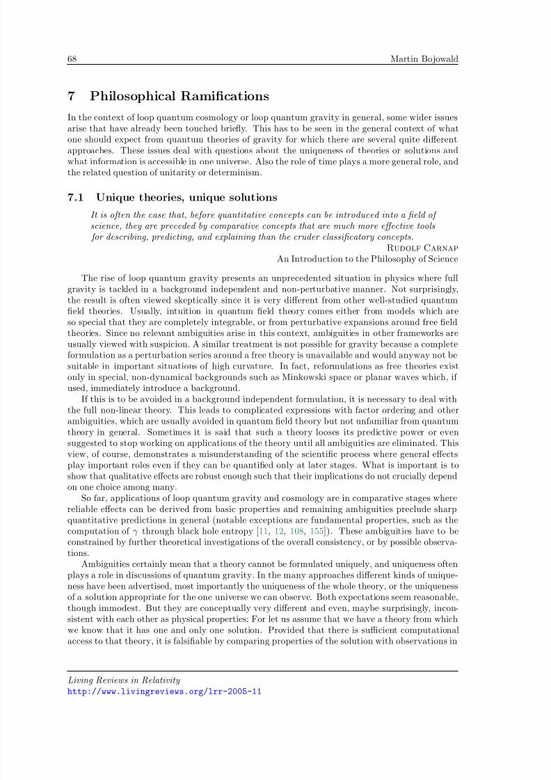
8/3/2019 Martin Bojowald- Loop Quantum Cosmology
http://slidepdf.com/reader/full/martin-bojowald-loop-quantum-cosmology 68/99
68 Martin Bojowald
7 Philosophical Ramifications
In the context of loop quantum cosmology or loop quantum gravity in general, some wider issuesarise that have already been touched briefly. This has to be seen in the general context of what
one should expect from quantum theories of gravity for which there are several quite differentapproaches. These issues deal with questions about the uniqueness of theories or solutions andwhat information is accessible in one universe. Also the role of time plays a more general role, andthe related question of unitarity or determinism.
7.1 Unique theories, unique solutions
It is often the case that, before quantitative concepts can be introduced into a field of science, they are preceded by comparative concepts that are much more effective tools for describing, predicting, and explaining than the cruder classificatory concepts.
Rudolf Carnap
An Introduction to the Philosophy of Science
The rise of loop quantum gravity presents an unprecedented situation in physics where fullgravity is tackled in a background independent and non-perturbative manner. Not surprisingly,the result is often viewed skeptically since it is very different from other well-studied quantumfield theories. Usually, intuition in quantum field theory comes either from models which areso special that they are completely integrable, or from perturbative expansions around free fieldtheories. Since no relevant ambiguities arise in this context, ambiguities in other frameworks areusually viewed with suspicion. A similar treatment is not possible for gravity because a completeformulation as a perturbation series around a free theory is unavailable and would anyway not besuitable in important situations of high curvature. In fact, reformulations as free theories existonly in special, non-dynamical backgrounds such as Minkowski space or planar waves which, if used, immediately introduce a background.
If this is to be avoided in a background independent formulation, it is necessary to deal with
the full non-linear theory. This leads to complicated expressions with factor ordering and otherambiguities, which are usually avoided in quantum field theory but not unfamiliar from quantumtheory in general. Sometimes it is said that such a theory looses its predictive power or evensuggested to stop working on applications of the theory until all ambiguities are eliminated. Thisview, of course, demonstrates a misunderstanding of the scientific process where general effectsplay important roles even if they can be quantified only at later stages. What is important is toshow that qualitative effects are robust enough such that their implications do not crucially dependon one choice among many.
So far, applications of loop quantum gravity and cosmology are in comparative stages wherereliable effects can be derived from basic properties and remaining ambiguities preclude sharpquantitative predictions in general (notable exceptions are fundamental properties, such as thecomputation of γ through black hole entropy [11, 12, 108, 155]). These ambiguities have to be
constrained by further theoretical investigations of the overall consistency, or by possible observa-tions.Ambiguities certainly mean that a theory cannot be formulated uniquely, and uniqueness often
plays a role in discussions of quantum gravity. In the many approaches different kinds of unique-ness have been advertised, most importantly the uniqueness of the whole theory, or the uniquenessof a solution appropriate for the one universe we can observe. Both expectations seem reasonable,though immodest. But they are conceptually very different and even, maybe surprisingly, incon-sistent with each other as physical properties: For let us assume that we have a theory from whichwe know that it has one and only one solution. Provided that there is sufficient computationalaccess to that theory, it is falsifiable by comparing properties of the solution with observations in
Living Reviews in Relativity http://www.livingreviews.org/lrr-2005-11

8/3/2019 Martin Bojowald- Loop Quantum Cosmology
http://slidepdf.com/reader/full/martin-bojowald-loop-quantum-cosmology 69/99
Loop Quantum Cosmology 69
the universe. Now, our observational access to the universe will always be limited and so, even if the one solution of our theory does agree with observations, we can always find ways to change thetheory without being in observational conflict. The theory thus cannot be unique. Changing it inthe described situation may only violate other, external conditions that are not observable.
The converse, that a unique theory cannot have a unique solution, follows by logically reversingthe above argument. However, one has to be careful about different notions of uniqueness of atheory. It is clear from the above argument that uniqueness of a theory can be realized only underexternal, such as mathematical, conditions, which always are a matter of taste and depend onexisting knowledge. Nevertheless, the statement seems to be supported by current realizations of quantum gravity. String theory is one example where the supposed uniqueness of the theory is faroutweighed by the non-uniqueness of its solutions. It should also be noted that the uniqueness of a theory is not falsifiable, and therefore not a scientific claim, unless its solutions are sufficientlyrestricted within the theory. Otherwise, one can always find new solutions if one comes in conflictwith observations. A theory itself, however, is falsifiable if it implies characteristic effects for itssolutions even though it may otherwise be ambiguous.
7.2 The role of time
Dies alles dauerte eine lange Zeit, oder eine kurze Zeit: denn, recht gesprochen, gibt es f¨ ur dergleichen Dinge auf Erden keine Zeit.
(All this took a long time, or a short time: for, strictly speaking, for such things notime on earth exists.)
Friedrich Nietzsche
Thus Spoke Zarathustra
Often, time is intuitively viewed as coordinate time, i.e., one direction of space-time. However,this does not have invariant physical meaning in general relativity, and conceptually an internaltime is more appropriate. Evolution is then measured in a relational manner of some degrees of
freedom with respect to others [33, 170, 106]. In quantum cosmology, as we have seen, this conceptis even more general since internal time keeps making sense at the quantum level also aroundsingularities where the classical space-time dissolves.
The wave function thus extends to a new branch beyond the classical singularity, i.e., to aclassically disconnected region. Intuitively this leads to a picture of a collapsing universe precedingthe Big Bang, but one has to keep in mind that this is the picture obtained from internal timewhere other time concepts are not available. In such a situation it is not clear, intuitive picturesnotwithstanding, how this transition would be perceived by observers were they able to withstandthe extreme conditions. It can be said reliably that the wave function is defined at both sides,“before” and “after”, and every computation of physical predictions, e.g., using observables, wecan do at “our” side can also be done at the other side. In this sense, quantum gravity is free of singularities and provides a transition between the two branches. The more complicated question
is what this means for evolution in a literal sense of our usual concept of time (see also [200]).Effective equations displaying bounces in coordinate time evolution indicate that indeed clas-sical singularities are replaced by a bouncing behavior. However, this does not occur completelygenerally and does not say anything about the orientation reversal which is characteristic for thequantum transition. In fact, effective equations describe the motion of semiclassical wave packets,which becomes less reliable at very small volume. And even if the effective bounce happens faraway from the classical singularity will there in general be a part of the wave function splitting off and traversing to the other orientation as can be seen in the example of Figure 10.
It is not clear in general that a wave function penetrating a classical singularity enters a newclassical regime even if the volume becomes large again. For instance, there can be oscillations
Living Reviews in Relativity http://www.livingreviews.org/lrr-2005-11
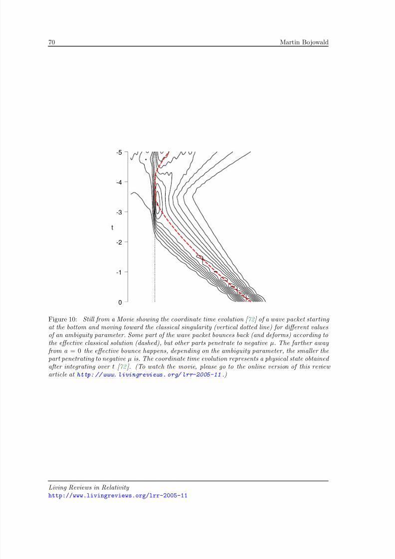
8/3/2019 Martin Bojowald- Loop Quantum Cosmology
http://slidepdf.com/reader/full/martin-bojowald-loop-quantum-cosmology 70/99
70 Martin Bojowald
0
-1
-2
-3
-4
-5
t
Figure 10: Still from a Movie showing the coordinate time evolution [ 72 ] of a wave packet starting at the bottom and moving toward the classical singularity (vertical dotted line) for different valuesof an ambiguity parameter. Some part of the wave packet bounces back (and deforms) according tothe effective classical solution (dashed), but other parts penetrate to negative µ. The farther away from a = 0 the effective bounce happens, depending on the ambiguity parameter, the smaller thepart penetrating to negative µ is. The coordinate time evolution represents a physical state obtained after integrating over t [ 72 ]. (To watch the movie, please go to the online version of this review article at http://www. livingreviews.org/ lrr-2005-11 .)
Living Reviews in Relativity http://www.livingreviews.org/lrr-2005-11
8/3/2019 Martin Bojowald- Loop Quantum Cosmology
http://slidepdf.com/reader/full/martin-bojowald-loop-quantum-cosmology 71/99
Loop Quantum Cosmology 71
on small scales, i.e., violations of pre-classicality, picked up by the wave function when it travelsthrough the classical singularity. As discussed in Section 5.17, the question of what conditionson a wave function to require for a classical regime is still open, but even if one can confidentlysay that there is such a new classical region does the question arise if time continues during thetransition through the pure quantum regime. At least in the special model of a free massless scalarin isotropic cosmology the answer to both questions is affirmative, based on the availability of aphysical inner product and quantum observables in this model [24].
Also related to this context is the question of unitary evolution. Even if one uses a selfadjointconstraint operator, unitary evolution is not guaranteed. First, the constraint splits into a timegenerator part containing derivatives or difference operators with respect to internal time and asource part containing, for instance, the matter Hamiltonian. It is then not guaranteed that thetime generator will lead to unitary evolution. Secondly, it is not obvious in what inner productto measure unitarity since the constraint is formulated in the kinematical Hilbert space but thephysical inner product is relevant for its solutions. This shows that the usual expectation of unitaryevolution, commonly motivated by preservation of probability or normalization of a wave functionin an absolute time parameter, is not reliable in quantum cosmology. It must be replaced by
suitable conditions on relational probabilities computed from physical wave functions.
7.3 Determinism
Hat die Zeit nicht Zeit? (Does time not have time? )Friedrich Nietzsche
Beyond Good and Evil
Loosely related to unitarity, but more general, is the concept of determinism. This is usuallyweakened in quantum mechanics anyway since in general one makes only probabilistic statements.Nevertheless, the wave function is determined at all times by its initial values, which is sometimesseen as the appropriate substitute for deterministic behavior. In loop quantum cosmology thesituation again changes slightly since, as discussed in Section 5.18, the wave function may not bedetermined by the evolution equation everywhere, i.e., not at points of classical singularities, andinstead acquire new conditions on its initial values. This could be seen as a form of indeterministicbehavior, even though the values of a wave function at classical singularities would not have anyeffect on the behavior for non-degenerate configurations.2 (If they had such an effect, the evolutionwould be singular.) In this situation one deals with determinism in a background independentcontext, which requires a new view.
In fact, rather than interpreting the freedom of choosing values at classical singularities asindeterministic behavior, it seems more appropriate to see this as an example for deterministic be-havior in a background independent theory. The internal time label µ first appears as a kinematicalobject through the eigenvalues of the triad operator (46). It then plays a role in the constraintequation (49) when formulated in the triad representation. Choosing internal time is just made forconvenience, and it is the constraint equation that must be used to see if this choice makes sense
in order to formulate evolution. This is indeed the case at non-zero µ where we obtain a differenceoperator in the evolution parameter. At zero µ, however, the operator changes and does not allowus to determine the wave function there from previous values. Now, we can interpret this simply asa consequence of the constraint equation rejecting the internal time value µ = 0. The backgroundindependent evolution selects the values of internal time it needs to propagate a wave functionuniquely. As it turns out, µ = 0 is not always necessary for this and thus simply decouples. Inhindsight, one could already have split off |0 from the kinematical Hilbert space, thereby removingthe classical singularity by hand. Since we did not do this, it is the evolution equation that tells
2The author thanks Christian Wuthrich for discussions.
Living Reviews in Relativity http://www.livingreviews.org/lrr-2005-11
8/3/2019 Martin Bojowald- Loop Quantum Cosmology
http://slidepdf.com/reader/full/martin-bojowald-loop-quantum-cosmology 72/99
72 Martin Bojowald
us that this is happening anyway. Recall, however, that this is only one possible scenario obtainedfrom a non-symmetric constraint. For the evolution (50) following from the symmetric constraint,no decoupling happens and µ = 0 is just like any other internal time value.
Living Reviews in Relativity http://www.livingreviews.org/lrr-2005-11
8/3/2019 Martin Bojowald- Loop Quantum Cosmology
http://slidepdf.com/reader/full/martin-bojowald-loop-quantum-cosmology 73/99
Loop Quantum Cosmology 73
8 Research Lines
Currently, the development of loop quantum cosmology proceeds along different lines, at all levelsdiscussed before. We present here a list of the main ones, ordered by topics rather than importance
or difficulty.
8.1 Conceptual issues
The list of conceptual issues is not much different from but equally pressing as in quantum gravityin general. Here, mainly the issue of time (its interpretation, different roles and explicit implemen-tation into physics), the interpretation of the wave function in quantum theory, and technical aswell as conceptual questions related to the physical inner product need to be addressed.
8.2 Mathematical development of models
The main open issue, requiring new insights at all levels, is that of inhomogeneities. While inho-
mogeneous models have been formulated and partly analyzed, the following tasks are still to becompleted:
Exact models: In particular the dynamics of inhomogeneous models is much more complicatedto analyze than in homogeneous ones. Understanding may be improved by an interestingcross-relation with black holes. This allows one to see if the different ingredients and effectsof a loop quantization fit together in a complete picture, which so far seems to be the case[14, 159, 13, 76, 57]. Moreover, the dynamics can possibly be simplified and understoodbetter around slowly evolving horizons [79, 76]. Other horizon conditions are also beingstudied in related approaches [132, 107].
Consistency: Not directly related to physical applications but equally important is the issueof consistency of the constraints. The constraint algebra trivializes in homogeneous models,
but is much more restrictive with inhomogeneities. Here, the feasibility of formulating aconsistent theory of quantum gravity can be tested in a treatable situation. Related toconsistency of the algebra, at least at a technical level, is the question of whether or notquantum gravity can predict initial conditions for a universe, or at least restrict its set of solutions.
Relation between models and the full theory: By strengthening the relation between mod-els and the full theory, ideally providing a complete derivation of models, physical applicationswill be put on a much firmer footing. This is also necessary to understand better effects of reductions such as degeneracies b etween different concepts or partial backgrounds. One as-pect not realized in models so far is the large amount of non-Abelian effects in the full theory,which can be significant also in models [54].
Numerical quantum gravity: Most systems of difference equations arising in loop quantumgravity are too complicated to solve exactly or even to analyze. Special techniques, such asthose in [72, 87, 71, 24, 88] have to be developed so as to apply to more general systems.In particular for including inhomogeneities, both for solving equations and interpreting solu-tions, a new area of numerical quantum gravity has to be developed.
Perturbations: If the relation between different models is known, as presently realized forisotropic within homogeneous models [63], one can formulate the less symmetric model per-turbatively around the more symmetric one. This then provides a simpler formulation of themore complicated system, easing the analysis and uncovering new effects. In this context,
Living Reviews in Relativity http://www.livingreviews.org/lrr-2005-11
8/3/2019 Martin Bojowald- Loop Quantum Cosmology
http://slidepdf.com/reader/full/martin-bojowald-loop-quantum-cosmology 74/99
74 Martin Bojowald
also alternative methods to introduce approximate symmetries, based on coherent states ase.g., advocated in [84], exist.
Effective equations: Finding effective equations that capture the quantum behavior of basic
difference equations, at least in some regimes, will be most helpful for a general analysis.However, their derivation is much more complicated for inhomogeneous systems owing to theconsistency issue. On the other hand, trying to derive them will provide important tests forthe framework, in addition to giving rise to new applications.
8.3 Applications
Once available, equations for inhomogeneous systems have the prospect of applications such as thefollowing.
Structure formation: There are diverse scenarios for the early universe with a potential forviable structure formation, which can only be checked with a reliable handle on inhomo-geneities. This applies to inflaton models with loop effects, inflation models without inflaton,
and the generation of structure before and subsequent propagation through a bounce.
Robustness: All results obtained so far have to be regarded as preliminary and their validity inthe presence of perturbative inhomogeneities has to be established. A detailed analysis of their robustness to quantization freedom such as ambiguities or choosing matter fields is stillto be undertaken.
New effects: Some cosmological issues that have not been addressed so far from loop quantumgravity, and which most likely require inhomogeneities, are: the initial state of the inflaton(Gaussianity) or the present acceleration of cosmic expansion. The latter could be a result of small, local quantum corrections adding up to a sizeable effect on the whole universe. Froma technical point of view, contact to quantum gravity phenomenology in a particle physicscontext can be made (as initially in [70]).
Ansatze: For the time being, those questions can be addressed preliminaryly by choosing suitableforms of inhomogeneous equations motivated by operators in full loop quantum gravity.
8.4 Homogeneous models
There are still several open areas in homogeneous models, which later can be extended to inhomo-geneous ones:
Conceptual issues: This has already been mentioned above. Isotropic models provide simplersettings to analyze, e.g., the physical inner product [127, 162, 24], observables, differentinterpretations of quantum aspects or the emergence of a classical world.
Effective equations: Even in isotropic models effective equations have not yet been derivedcompletely. A general scheme exists, shown to be analogous to standard effective actiontechniques [73], but it remains to be applied completely to quantum cosmology. This willthen lead to a complete set of correction terms and their ranges of validity and importance.Also the question of whether an effective action for quantum cosmology exists and what itsform is can be addressed.
Matter systems: Matter systems provide a rich source of diverse scenarios, but a full analysisis yet to be done. This includes adding different kinds of fluids [163], fermions or anisotropyparameters (shear term).
Living Reviews in Relativity http://www.livingreviews.org/lrr-2005-11
8/3/2019 Martin Bojowald- Loop Quantum Cosmology
http://slidepdf.com/reader/full/martin-bojowald-loop-quantum-cosmology 75/99
Loop Quantum Cosmology 75
8.5 Outlook
All these developments will certainly also aid and suggest developments in the full theory, andreciprocally be assisted by new ideas realized there. At the other side, guidance as well as means
for testing can be expected from future observations.
Living Reviews in Relativity http://www.livingreviews.org/lrr-2005-11
8/3/2019 Martin Bojowald- Loop Quantum Cosmology
http://slidepdf.com/reader/full/martin-bojowald-loop-quantum-cosmology 76/99
76 Martin Bojowald
A Invariant connections
We first fix our notation by describing the additional structure provided by a given action of asymmetry group on a space manifold. This allows us to review the mathematical classification of principal fiber bundles carrying an action of a symmetry group, and their invariant connections.
A.1 Partial backgrounds
To describe a theory of connections we need to fix a principal fiber bundle P (Σ, G , π) over theanalytic base manifold Σ with compact structure group G. Let S < Aut(P ) be a Lie symmetrysubgroup of bundle automorphisms acting on the principal fiber bundle P . Using the bundleprojection π : P → Σ we get a symmetry operation of S on Σ. For simplicity we will assume thatall orbits of S are of the same type. If necessary we will have to decompose the base manifold intoseveral orbit bundles Σ(F ) ⊂ Σ, where F ∼= S x is the isotropy subgroup of S consisting of elementsfixing a point x of the orbit bundle Σ(F ) (isotropy subgroups for different points in Σ(F ) are notidentical but conjugate to each other). This amounts to a special treatment of possible symmetry
axes or centers.By restricting ourselves to one fixed orbit bundle we fix an isotropy subgroup F ≤ S up to
conjugacy, and we require that the action of S on Σ is such that the orbits are given by S (x) ∼= S/F for all x ∈ Σ. This will be the case if S is compact but also in most other cases of physical interest.Moreover, we will have to assume later on that the coset space S/F is reductive [138, 139], i.e.,that LS can be written as a direct sum LS = LF ⊕ LF ⊥ with AdF (LF ⊥) ⊂ LF ⊥. If S issemisimple, LF ⊥ is the orthogonal complement of LF with respect to the Cartan–Killing metricon LS . Further examples are provided by freely acting symmetry groups, in which case we haveF = 1, and semidirect products of the form S = N F , where LF ⊥ = LN . The latter cases arerelevant for homogeneous and isotropic cosmological models.
The base manifold can be decomposed as Σ ∼= Σ/S × S/F where Σ/S ∼= B ⊂ Σ is the basemanifold of the orbit bundle and can be realized as a submanifold B of Σ via a section in this
bundle. As already noted in the main text, the action of a symmetry group on space introduces apartial background into the model. In particular, full diffeomorphism invariance is not preservedbut reduced to diffeomorphisms only on the reduced manifold B. To see what kind of partialbackground we have in a model it is helpful to contrast the mathematical definition of symmetryactions with the physical picture.
To specify an action of a group on a manifold one has to give, for each group element, a mapbetween space points satisfying certain conditions. Mathematically, each point is uniquely deter-mined by labels, usually by coordinates in a chosen (local) coordinate system. The group actioncan then be written down in terms of maps of the coordinate charts, and there are compatibilityconditions for maps expressed in different charts to ensure that the ensuing map on the manifoldis coordinate independent. If we have active diffeomorphism invariance, however, individual pointsin space are not well-defined. This leads to the common view that geometrical observables suchas the area of a surface are, for physical purposes, not actually defined by integrating over a sub-manifold simply in parameter form, but over subsets of space defined by the values of matter fields[171, 169]. Since matter fields are subject to diffeomorphisms just as the metric, area defined insuch a manner is diffeomorphism invariant.
Similarly, orbits of the group action are not to be regarded as fixed submanifolds, but as beingdeformed by diffeomorphisms. Fixing a class of orbits filling the space manifold Σ correspondsto selecting a special coordinate system adapted to the symmetry. For instance, in a sphericallysymmetric situation one usually chooses spherical coordinates (r,ϑ,ϕ), where r > 0 labels theorbits and ϑ and ϕ are angular coordinates and can be identified with some parameters of thesymmetry group SO(3). In a Euclidean space the orbits can be embedded as spheres S 2 of constant
Living Reviews in Relativity http://www.livingreviews.org/lrr-2005-11
8/3/2019 Martin Bojowald- Loop Quantum Cosmology
http://slidepdf.com/reader/full/martin-bojowald-loop-quantum-cosmology 77/99
Loop Quantum Cosmology 77
curvature. Applying a diffeomorphism, however, will deform the spheres and they are in generalonly topological S 2. Physically, the orbits can be specified as level surfaces of matter fields, similarto specifying space points. This concept allows us to distinguish in a diffeomorphism invariantmanner between curves (such as edges of spin networks) that are tangential and curves that aretransversal to the group orbits.
It is, however, not possible to label single points in a given orbit in such a physical manner,simply because we could not introduce the necessary matter fields without destroying the symmetry.Thus we have to use the action of the symmetry group, which provides us with additional structure,to label the points, e.g., by using the angular coordinates in the example above. A similar role isplayed by the embedding of the reduced manifold B into Σ by choosing a section of the orbit bundle,which provides a base point for each orbit (a north pole in the example of spherical symmetry).This amounts to a partial fixing of the diffeomorphism invariance by allowing only diffeomorphismsthat respect the additional structure. The reduced diffeomorphism constraint will then in generalrequire only invariance with respect to diffeomorphisms of the manifold B.
In a reduced model, a partial fixing of the diffeomorphism invariance does not cause problemsbecause all fields are constant along the orbits anyway. However, if we study symmetric states
as generalized states of the full theory, as in Section 6, we inevitably have to break partially thediffeomorphism invariance. The distributional evaluation of symmetric states and the dual actionof basic operators thus depends on the partial background provided by the symmetry.
A.2 Classification of symmetric principal fiber bundles
Fields that are invariant under the action of a symmetry group S on space Σ are defined by a setof linear equations for invariant field components. Nevertheless, finding invariant fields in gaugetheories is not always straightforward since, in general, fields need to be invariant only up togauge transformations which depend on the symmetry transformation. An invariant connection,for instance, satisfies the equation
s∗A = g(s)−1Ag(s) + g(s)−1dg(s) (66)
with a local gauge transformation g(s) for each s ∈ S . These gauge transformations are notarbitrary since two symmetry transformations s1 and s2 applied one after another have to implya gauge transformation with g(s2s1) related to g(s1) and g(s2). However, this does not simplyamount to a homomorphism property and allowed maps g : S → G are not easily determined bygroup theory. Thus, even though for a known map g one simply has to solve a system of linearequations for A, finding appropriate maps g can be difficult. In most cases, the equations wouldnot have any non-vanishing solution at all, which would certainly be insufficient for interestingreduced field theories.
In the earlier physical literature, invariant connections and other fields have indeed been deter-mined by trial and error [91], but the same problem has been solved in the mathematical literature[138, 139, 82] in impressive generality. This uses the language of principal fiber bundles which
already provides powerful techniques. Moreover, the problem of solving one system of equationsfor A and g(s) at the same time is split into two separate problems, which allows a more systematicapproach. The first step is to realize that a connection whose local 1-forms A on Σ are invariant upto gauge is equivalent to a connection 1-form ω defined on the full fiber bundle P , which satisfiesthe simple invariance conditions s∗ω = ω for all s ∈ S . This is indeed simpler to analyze since wenow have a set of linear equations for ω alone. However, even though hidden in the notation, themap g : S → G is still present. The invariance conditions for ω defined on P are well-defined onlyif we know a lift from the original action of S on the base manifold Σ to the full bundle P . As withmaps g : S → G, there are several inequivalent choices for the lift which have to be determined.The advantage of this procedure is that this can be done by studying symmetric principal fiber
Living Reviews in Relativity http://www.livingreviews.org/lrr-2005-11
8/3/2019 Martin Bojowald- Loop Quantum Cosmology
http://slidepdf.com/reader/full/martin-bojowald-loop-quantum-cosmology 78/99
78 Martin Bojowald
bundles, i.e., principal fiber bundles carrying the action of a symmetry group, independently of the behavior of connections. In a second step, one can then ask what form invariant connectionson a given symmetric principal fiber bundle have.
We now discuss the first step of determining lifts of the symmetry action of S from Σ to P .Given a point x ∈ Σ, the action of the isotropy subgroup F yields a map F : π−1(x) → π−1(x)of the fiber over x, which commutes with the right action of G on the bundle. To each point p ∈ π−1(x) we can assign a group homomorphism λ p : F → G defined by f ( p) =: p · λ p(f ) for allf ∈ F . To verify this we first note that commutativity of the action of S < Aut(P ) with rightmultiplication of G on P implies that we have the conjugate homomorphism λ p = Adg−1 λ p fora different point p = p · g in the same fiber:
p · λ p(f ) = f ( p · g) = f ( p) · g = ( p · λ p(f )) · g = p · Adg−1λ p(f ).
This yields
(f 1 f 2)( p) = f 1( p · λ p(f 2)) = ( p · λ p(f 2)) · Adλp(f 2)−1λ p(f 1) = p · (λ p(f 1) · λ p(f 2))
demonstrating the homomorphism property. We thus obtain a map λ : P × F → G, ( p,f ) → λ p(f )obeying the relation λ p·g = Adg−1 λ p.
Given a fixed homomorphism λ : F → G, we can build the principal fiber subbundle
Qλ(B, Z λ, πQ) := p ∈ P |B : λ p = λ (67)
over the base manifold B, which as structure group has the centralizer
Z λ := Z G(λ(F )) = g ∈ G : gf = f g for all f ∈ λ(F )
of λ(F ) in G. P |B is the restricted fiber bundle over B. A conjugate homomorphism λ = Adg−1 λsimply leads to an isomorphic fiber bundle.
The structure elements [λ] and Q classify symmetric principal fiber bundles according to the
following theorem [82]:
Theorem 1 An S -symmetric principal fiber bundle P (Σ, G , π) with isotropy subgroup F ≤ S of theaction of S on Σ is uniquely characterized by a conjugacy class [λ] of homomorphisms λ : F → Gtogether with a reduced bundle Q(Σ/S,Z G(λ(F )), πQ).
Given two groups F and G we can make use of the relation [81]
Hom(F, G)/Ad ∼= Hom(F, T (G))/W (G) (68)
in order to determine all conjugacy classes of homomorphisms λ : F → G. Here, T (G) is a maximaltorus and W (G) the Weyl group of G. Different conjugacy classes correspond to different sectorsof the theory, which can be interpreted as having different topological charge. In spherically
symmetric electromagnetism, for instance, this is just magnetic charge [35, 66].
A.3 Classification of invariant connections
Now let ω be an S -invariant connection on the symmetric bundle P classified by ([λ], Q), i.e.,s∗ω = ω for any s ∈ S . After restriction, ω induces a connection ω on the reduced bundle Q.Because of S -invariance of ω the reduced connection ω is a one-form on Q with values in the Liealgebra of the reduced structure group. To see this, fix a point p ∈ P and a vector v in T pP such that π∗v ∈ σ∗T π( p)B, where σ is the embedding of B into Σ. Such a vector, which does nothave components along symmetry orbits, is fixed by the action of the isotropy group: df (v) = v.
Living Reviews in Relativity http://www.livingreviews.org/lrr-2005-11

8/3/2019 Martin Bojowald- Loop Quantum Cosmology
http://slidepdf.com/reader/full/martin-bojowald-loop-quantum-cosmology 79/99
Loop Quantum Cosmology 79
The pull back of ω by f ∈ F applied to v is by definition f ω p(v) = ωf ( p)(df (v)) = ωf ( p)(v).Now using the fact that f acts as gauge transformation in the fibers and observing the definitionof λ p and the adjoint transformation of ω, we obtain ωf ( p)(v) = Adλp(f )−1ω p(v). By assumptionthe connection ω is S -invariant implying f ω p(v) = Adλ
p(f
)
−1ω p(v) = ω p(v) for all f ∈
F . Thisshows that ω p(v) ∈ LZ G(λ p(F )), and ω can be restricted to a connection on the bundle Qλ withstructure group Z λ.
Furthermore, using ω we can construct the linear map Λ p : LS → LG, X → ω p(X ) for any
p ∈ P . Here, X is the vector field on P given by X (h) := d(exp(tX )h)/dt|t=0 for any X ∈LS and h ∈ C 1(P,R). For X ∈ LF the vector field X is a vertical vector field, and we haveΛ p(X ) = dλ p(X ), where dλ : LF → LG is the derivative of the homomorphism defined above.This component of Λ is therefore already given by the classifying structure of the principal fiberbundle. Using a suitable gauge, λ can be held constant along B. The remaining componentsΛ p|LF ⊥ yield information about the invariant connection ω. They are subject to the condition
Λ p(Adf (X )) = Adλp(f )(Λ p(X )) for f ∈ F, X ∈ LS, (69)
which follows from the transformation of ω under the adjoint representation and which provides aset of equations determining the form of the components Λ.Keeping only the information characterizing ω we have, besides ω, the scalar field φ : Q →
LG ⊗ LF ⊥, which is determined by Λ p|LF ⊥ and can be regarded as having dim LF ⊥ componentsof LG-valued scalar fields. The reduced connection and the scalar field suffice to characterize aninvariant connection [82]:
Theorem 2 (Generalized Wang Theorem) Let P (Σ, G) be an S -symmetric principal fiber bun-dle classified by ([λ], Q) according to Theorem 1, and let ω be an S -invariant connection on P .
Then the connection ω is uniquely classified by a reduced connection ω on Q and a scalar fieldφ : Q × LF ⊥ → LG obeying Equation ( 69 ).
In general, φ transforms under some representation of the reduced structure group Z λ: Its
values lie in the subspace of LG determined by Equation (69) and form a representation spacefor all group elements of G (which act on Λ) whose action preserves the subspace. These are bydefinition precisely elements of the reduced group.
The connection ω can be reconstructed from its classifying structure (ω, φ) as follows: Accordingto the decomposition Σ ∼= B × S/F we have
ω = ω + ωS/F , (70)
where ωS/F is given by Λ ιθMC in a gauge depending on the (local) embedding ι : S/F → S .Here θMC is the Maurer–Cartan form on S taking values in LS . Through Λ, ω depends on λ andφ.
Living Reviews in Relativity http://www.livingreviews.org/lrr-2005-11
8/3/2019 Martin Bojowald- Loop Quantum Cosmology
http://slidepdf.com/reader/full/martin-bojowald-loop-quantum-cosmology 80/99
80 Martin Bojowald
B Examples
With these general results we can now quickly derive the form of invariant connections for thecases studied in the main text.
B.1 Homogeneous models
In Bianchi models the transitive symmetry group acts freely on Σ, which implies that Σ canlocally be identified with the group manifold S . The three generators of LS will be denoted as T I ,1 ≤ I ≤ 3, with relations [T I , T J ] = C KIJ T K , where C KIJ are the structure constants of LS fulfillingC J IJ = 0 for class A models by definition. The Maurer–Cartan form on S is given by θMC = ωI T I with left invariant one-forms ωI on S , which fulfill the Maurer–Cartan equations
dωI = −12
C I JKωJ ∧ ωK . (71)
Due to F = 1, all homomorphisms λ : F → G are given by 1 → 1, and we can use the embeddingι = id: S/F → S . An invariant connection then takes the form A = φ θMC = φiI τ iω
I = Aiaτ idxa
with matrices τ i generating LSU(2). The scalar field is given by φ : LS → LG, T I → φ(T I ) =: φiI τ ialready in its final form, because condition (69) is empty for a trivial isotropy group.
Using left invariant vector fields X I obeying ωI (X J ) = δI J and with Lie brackets [X I , X J ] =
C KIJ X K the momenta canonically conjugate to Aia = φiI ω
I a can be written as E ai =
√g0 ˜ pI i X aI with
˜ pI i being canonically conjugate to φiI . Here, g0 = det(ωI a)2 is the determinant of the left invariant
metric (g0)ab :=
I ωI aωI
b on Σ, which is used to provide the density weight of E ai . The symplecticstructure can be derived from
1
8πγG
Σ
d3x AiaE ai =
1
8πγG
Σ
d3x√
g0˙φiI ˜ p
J i ωI (X J ) =
V 08πγG
˙φiI ˜ pI i ,
to obtainφiI , ˜ pJ j = 8πγGV 0δijδJ I (72)
with the volume V 0 := Σ d3x√g0 of Σ measured with the invariant metric g0.It is convenient to absorb the coordinate volume V 0 into the fields by redefining φiI := V
1/30 φiI
and pI i := V 2/30 ˜ pI i . This makes the symplectic structure independent of V 0 in accordance with
background independence. These redefined variables automatically appear in holonomies andfluxes through coordinate integrations.
B.2 Isotropic models
On Bianchi models, additional symmetries can be imposed, which corresponds to a further sym-metry reduction and introduces non-trivial isotropy subgroups. These models with enhanced sym-metry can be treated on an equal footing by writing the symmetry group as a semidirect productS = N ρ F , with the isotropy subgroup F and the translational subgroup N , which is one of
the Bianchi groups. Composition in this group is defined as (n1, f 1)(n2, f 2) := (n1ρ(f 1)(n2), f 1f 2),which depends on the group homomorphism ρ : F → AutN into the automorphism group of N (which will be denoted by the same letter as the representation on AutLN used below). Inverse ele-ments are given by (n, f )−1 = (ρ(f −1)(n−1), f −1). To determine the form of invariant connectionswe have to compute the Maurer–Cartan form on S (using the usual notation):
θ(S)MC(n, f ) = (n, f )−1d(n, f ) = (ρ(f −1)(n−1), f −1)(dn, df )
= (ρ(f −1)(n−1)ρ(f −1)(dn), f −1df ) = (ρ(f −1)(n−1dn), f −1df )
=
ρ(f −1)(θ(N )MC(n)), θ(F )
MC(f )
. (73)
Living Reviews in Relativity http://www.livingreviews.org/lrr-2005-11
8/3/2019 Martin Bojowald- Loop Quantum Cosmology
http://slidepdf.com/reader/full/martin-bojowald-loop-quantum-cosmology 81/99
Loop Quantum Cosmology 81
Here the Maurer–Cartan forms θ(N )MC on N and θ
(F )MC on F appear. We then choose an embedding
ι : S/F = N → S , which can most easily be done as ι : n → (n, 1). Thus, ι∗θ(S)MC = θ
(N )MC , and a
reconstructed connection takes the form φ ι∗θ(S)MC = φiI ω
I τ i, which is the same as for anisotropic
models before (where now ωI
are left invariant one-forms on the translation group N ). However,here φ is constrained by equation (69) and we get only a subset as isotropic connections.
To solve Equation (69) we have to treat LRS (locally rotationally symmetric) models with asingle rotational symmetry and isotropic models separately. In the first case we choose LF = τ 3,whereas in the second case we have LF = τ 1, τ 2, τ 3 (· denotes the linear span). Equation (69)can be written infinitesimally as
φ(adτ i(T I )) = addλ(τ i)φ(T I ) = [dλ(τ i), φ(T I )]
(i = 3 for LRS, 1 ≤ i ≤ 3 for isotropy). The T I are generators of LN = LF ⊥, on whichthe isotropy subgroup F acts by rotation, adτ i(T I ) = iIKT K . This is the derivative of therepresentation ρ defining the semidirect product S : Conjugation on the left hand side of (69) isAd(1,f )(n, 1) = (1, f )(n, 1)(1, f −1) = (ρ(f )(n), 1), which follows from the composition in S .
Next, we have to determine the possible conjugacy classes of homomorphisms λ : F → G. ForLRS models their representatives are given by
λk : U(1) → SU(2), exp tτ 3 → exp ktτ 3
for k ∈ N0 = 0, 1, . . . (as will be shown in detail below for spherically symmetric connections). Forthe components φiI of φ defined by φ(T I ) = φiI τ i, Equation (69) takes the form 3IK φjK = k3lj φlI .
This has a non-trivial solution only for k = 1, in which case φ can be written as
φ1 = aτ 1 + bτ 2, φ2 = −bτ 1 + aτ 2, φ3 = cτ 3
with arbitrary numbers a, b, c (the factors of 2−12 are introduced for the sake of normalization).
Their conjugate momenta take the form
˜ p1 = 1
2
(˜ paτ 1 + ˜ pbτ 2), ˜ p2 = 1
2
(
−˜ pbτ 1 + ˜ paτ 2), ˜ p3 = ˜ pcτ 3,
and the symplectic structure is given by
a, ˜ pa = b, ˜ pb = c, ˜ pc = 8πγGV 0
and vanishes in all other cases. There is remaining gauge freedom from the reduced structure group
Z λ ∼= U(1) which rotates the pairs (a, b) and (˜ pa, ˜ pb). Gauge invariant are then only
a2 + b2 and
its momentum (a˜ pa + b˜ pb)/
a2 + b2.In the case of isotropic models we have only two homomorphisms λ0 : SU(2) → SU(2), f → 1
and λ1 = id up to conjugation (to simplify notation we use the same letters for the homomorphismsas in the LRS case, which is justified by the fact that the LRS homomorphisms are restrictionsof those appearing here). Equation (69) takes the form iIK φjK = 0 for λ0 without non-trivial
solutions, and iIK φjK = ilj φlI for λ1. Each of the last equations has the same form as for LRS
models with k = 1, and their solution is φiI = cδiI with an arbitrary c. In this case the conjugatemomenta can be written as ˜ pI i = ˜ pδI i , and we have the symplectic structure c, ˜ p = 8π
3GγV 0.
Thus, in both cases there is a unique non-trivial sector, and no topological charge appears. The
symplectic structure can again be made independent of V 0 by redefining a := V 1/30 a, b := V
1/30 b,
c := V 1/3
0 c and pa := V 2/3
0 ˜ pa, pb := V 2/3
0 ˜ pb, pc := V 2/3
0 ˜ pc, p := V 2/3
0 ˜ p. If one computes theisotropic reduction of a Bianchi IX metric following from the left-invariant 1-forms of SU(2), oneobtains a closed Friedmann–Robertson–Walker metric with scale factor a = 2a = 2
|˜ p| (see, e.g.,
[36] for the calculation). Thus, we obtain the identification (18) used in isotropic loop cosmology.(Such a normalization can only be obtained in curved models.)
Living Reviews in Relativity http://www.livingreviews.org/lrr-2005-11
8/3/2019 Martin Bojowald- Loop Quantum Cosmology
http://slidepdf.com/reader/full/martin-bojowald-loop-quantum-cosmology 82/99
82 Martin Bojowald
B.3 Spherical symmetry
In the generic case (i.e., outside a symmetry center) of spherical symmetry we have S = SU(2),F = U(1) = exp
τ 3
(
·denotes the linear span), and the connection form can be gauged to be
AS/F = (Λ(τ 2)sin ϑ + Λ(τ 3)cos ϑ) dϕ + Λ(τ 1)dϑ. (74)
Here (ϑ, ϕ) are (local) coordinates on S/F ∼= S 2 and as usually we use the basis elements τ iof LS . Λ(τ 3) is given by dλ, whereas Λ(τ 1,2) are the scalar field components. Equation (74)contains as special cases the invariant connections found in [91]. These are gauge equivalentby gauge transformations depending on the angular coordinates (ϑ, ϕ), i.e., they correspond tohomomorphisms λ that are not constant on the orbits of the symmetry group.
In order to specify the general form (74) further, the first step is again to find all conjugacyclasses of homomorphisms λ : F = U(1) → SU(2) = G. To do so we can make use of Equation (68)to which end we need the following information about SU(2) (see, e.g., [81]): The standard maximaltorus of SU(2) is given by
T (SU(2)) = diag(z, z−1
) : z ∈ U(1) ∼= U(1)and the Weyl group of SU(2) is the permutation group of two elements, W (SU(2)) ∼= S 2, itsgenerator acting on T (SU(2)) by diag(z, z−1) → diag(z−1, z).
All homomorphisms in Hom(U(1), T (SU(2))) are given by
λk : z → diag(zk, z−k)
for any k ∈ Z, and we have to divide out the action of the Weyl group leaving only the maps λk,k ∈ N0, as representatives of all conjugacy classes of homomorphisms. We see that spherically sym-metric gravity has a topological charge taking values in N0 (but only if degenerate configurationsare allowed, as we will see below).
We will represent F as the subgroup expτ 3 < SU(2) of the symmetry group S , and use thehomomorphisms λk : exp tτ 3
→exp ktτ 3 out of each conjugacy class. This leads to a reduced
structure group Z G(λk(F )) = expτ 3 ∼= U(1) for k = 0 and Z G(λ0(F )) = SU(2) (k = 0; this isthe sector of manifestly invariant connections of [92]). The map Λ|LF is given by dλk : τ 3 →LG, τ 3 → kτ 3, and the remaining components of Λ, which give us the scalar field, are determinedby Λ(τ 1, 2) ∈ LG subject to Equation (69), which here can be written as
Λ adτ 3 = addλ(τ 3) Λ.
Using adτ 3τ 1 = τ 2 and adτ 3τ 2 = −τ 1 we obtain
Λ(a0τ 2 − b0τ 1) = k(a0[τ 3, Λ(τ 1)] + b0[τ 3, Λ(τ 2)]),
where a0τ 1 + b0τ 2, a0, b0 ∈ R is an arbitrary element of LF ⊥. Since a0 and b0 are arbitrary, this isequivalent to the two equations
k[τ 3, Λ(τ 1)] = Λ(τ 2), k[τ 3, Λ(τ 2)] = −Λ(τ 1).
A general ansatz
Λ(τ 1) = a1τ 1 + b1τ 2 + c1τ 3 , Λ(τ 2) = a2τ 1 + b2τ 2 + c2τ 3
with arbitrary parameters ai, bi, ci ∈ R yields
k(a1τ 2 − b1τ 1) = a2τ 1 + b2τ 2 + c2τ 3,
k(−a2τ 2 + b2τ 1) = a1τ 1 + b1τ 2 + c1τ 3
Living Reviews in Relativity http://www.livingreviews.org/lrr-2005-11
8/3/2019 Martin Bojowald- Loop Quantum Cosmology
http://slidepdf.com/reader/full/martin-bojowald-loop-quantum-cosmology 83/99
Loop Quantum Cosmology 83
which have non-trivial solutions only if k = 1, namely
b2 = a1, a2 = −b1, c1 = c2 = 0.
The configuration variables of the system are the above fields a,b,c : B → R of the U(1)-connection form A = c(x) τ 3 dx on the one hand and the two scalar field components
Λ|τ 1 : B → LSU(2),
x → a(x)τ 1 + b(x)τ 2 =1
2
0 −b(x) − ia(x)
b(x) − ia(x) 0
=:
0 −w(x)
w(x) 0
on the other hand. Under a local U(1)-gauge transformation z(x) = exp(t(x)τ 3) they transform asc → c + dt/dx and w(x) → exp(−it)w, which can be read off from
A → z−1Az + z−1dz = A + τ 3dt,
Λ(τ 1)
→z−1Λ(τ 1)z =
0 − exp(it)w
exp(−it)w 0 .
In order to obtain a standard symplectic structure (see Equation (77) below), we reconstructthe general invariant connection form
A(x,ϑ,ϕ) = A1(x)τ 3dx + (A2(x)τ 1 + A3(x)τ 2)dϑ (75)
+ (A2(x)τ 2 − A3(x)τ 1)sin ϑ dϕ + cos ϑ dϕ τ 3.
An invariant densitized triad field is analogously given by
(E x, E ϑ, E ϕ) = (E 1 sin ϑ τ 3, 12
sin ϑ(E 2τ 1 + E 3τ 2), 12
(E 2τ 2 − E 3τ 1)) (76)
with coefficients E I canonically conjugate to AI (E 2 and E 3 are non-vanishing only for k = 1).
The symplectic structure AI (x), E J (y) = 2γGδJ I δ(x, y) (77)
can be derived by inserting the invariant expressions into (8 πγG)−1
Σd3xAi
aE ai .Information about the topological charge k can be found by expressing the volume in terms of
the reduced triad coefficients E I : Using
abcijkE ai E bjE ck = −2abc tr(E a[E b, E c]) = 32
sin2 ϑE 1
(E 2)2 + (E 3)2
(78)
we have
V =
Σ
d3x
16
abcijkE iaE jbE kc
= 2π
B
dx
|E 1|((E 2)2 + (E 3)2). (79)
We can now see that in all the sectors with k = 1 the volume vanishes because then E 2 = E 3 = 0.
All these degenerate sectors have to be rejected on physical grounds and we arrive at a uniquesector of invariant connections given by the parameter k = 1.
Living Reviews in Relativity http://www.livingreviews.org/lrr-2005-11
8/3/2019 Martin Bojowald- Loop Quantum Cosmology
http://slidepdf.com/reader/full/martin-bojowald-loop-quantum-cosmology 84/99
84 Martin Bojowald
References
[1] Alexander, S., “A Quantum Gravitational Relaxation of The Cosmological Constant”,(2005). URL (cited on 09 October 2005):
http://arXiv.org/abs/hep-th/0503146. 2
[2] Alexander, S., Malecki, J., and Smolin, L., “Quantum Gravity and Inflation”, Phys. Rev. D,70, 044025, (2004). Related online version (cited on 09 October 2005):http://arXiv.org/abs/hep-th/0309045. 2
[3] Alfaro, J., Morales-Tecotl, H.A., and Urrutia, L.F., “Quantum gravity corrections to neutrinopropagation”, Phys. Rev. Lett., 84, 2318–2321, (2000). Related online version (cited on 09October 2005):http://arXiv.org/abs/gr-qc/9909079. 4.12
[4] Alfaro, J., Morales-Tecotl, H.A., and Urrutia, L.F., “Loop quantum gravity and light propa-gation”, Phys. Rev. D, 65, 103509, (2002). Related online version (cited on 09 October 2005):
http://arXiv.org/abs/hep-th/0108061. 4.12
[5] Anninos, P., “Computational Cosmology: From the Early Universe to the Large Scale Struc-ture”, Living Rev. Relativity , 4, lrr-2001-2, (2001). URL (cited on 09 October 2005):http://www.livingreviews.org/lrr-2001-2. 4
[6] Arnowitt, R., Deser, S., and Misner, C.W., “The dynamics of general relativity”, in Witten,L., ed., Gravitation: An Introduction to Current Research , 227–265, (Wiley, New York,U.S.A., 1962). 3.1
[7] Ashtekar, A., “New Variables for Classical and Quantum Gravity”, Phys. Rev. Lett., 57,2244–2247, (1986). 3.2
[8] Ashtekar, A., “New Hamiltonian Formulation of General Relativity”, Phys. Rev. D, 36(6),
1587–1602, (1987). 3.2
[9] Ashtekar, A., “Quantum Geometry and Gravity: Recent Advances”, in Bishop, N.T., andMaharaj, S.D., eds., General Relativity and Gravitation , Proceedings of the 16th Interna-tional Conference on General Relativity and Gravitation, Durban, South Africa, 15–21 July2001, (World Scientific, Singapore; River Edge, U.S.A., 2002). Related online version (citedon 09 October 2005):http://arXiv.org/abs/gr-qc/0112038. 3
[10] Ashtekar, A., “Quantum Geometry In Action: Big Bang and Black Holes”, in Lyubich,M., and Takhtajan, L., eds., Graphs and Patterns in Mathematics and Theoretical Physics,Proceedings of the conference dedicated to Dennis Sullivan’s 60th birthday, June 14–21, 2001,Stony Brook University, Stony Brook, NY, (American Mathematical Society, Providence,
U.S.A., 2002). Related online version (cited on 09 October 2005):http://arXiv.org/abs/math-ph/0202008. 3
[11] Ashtekar, A., Baez, J.C., Corichi, A., and Krasnov, K.V., “Quantum Geometry and BlackHole Entropy”, Phys. Rev. Lett., 80, 904–907, (1998). Related online version (cited on 09October 2005):http://arXiv.org/abs/gr-qc/9710007. 3.3, 7.1
[12] Ashtekar, A., Baez, J.C., and Krasnov, K.V., “Quantum Geometry of Isolated Horizons andBlack Hole Entropy”, Adv. Theor. Math. Phys., 4, 1–94, (2000). Related online version (cited
Living Reviews in Relativity http://www.livingreviews.org/lrr-2005-11
8/3/2019 Martin Bojowald- Loop Quantum Cosmology
http://slidepdf.com/reader/full/martin-bojowald-loop-quantum-cosmology 85/99
Loop Quantum Cosmology 85
on 09 October 2005):http://arXiv.org/abs/gr-qc/0005126. 3.3, 7.1
[13] Ashtekar, A., and Bojowald, M., “Black hole evaporation: A paradigm”, Class. Quantum
Grav., 22, 3349–3362, (2005). Related online version (cited on 09 October 2005):http://arXiv.org/abs/gr-qc/0504029. 8.2
[14] Ashtekar, A., and Bojowald, M., “Quantum Geometry and the Schwarzschild Singularity”,(2005). URL (cited on 09 October 2005):http://arXiv.org/abs/gr-qc/0509075. 5.8, 5.12, 8.2
[15] Ashtekar, A., Bojowald, M., and Lewandowski, J., “Mathematical structure of loop quantumcosmology”, Adv. Theor. Math. Phys., 7, 233–268, (2003). Related online version (cited on09 October 2005):http://arXiv.org/abs/gr-qc/0304074. 4.2, 5.2, 5.4, 5.5
[16] Ashtekar, A., Bojowald, M., and Willis, J., in preparation. 5.5.2
[17] Ashtekar, A., Corichi, A., and Zapata, J.A., “Quantum Theory of Geometry III: Non-commutativity of Riemannian Structures”, Class. Quantum Grav., 15, 2955–2972, (1998).Related online version (cited on 09 October 2005):http://arXiv.org/abs/gr-qc/9806041. 3.3
[18] Ashtekar, A., Fairhurst, S., and Willis, J.L., “Quantum gravity, shadow states, and quantummechanics”, Class. Quantum Grav., 20, 1031–1062, (2003). Related online version (cited on09 October 2005):http://arXiv.org/abs/gr-qc/0207106. 4.3, 5.2
[19] Ashtekar, A., and Lewandowski, J., “Projective Techniques and Functional Integration forGauge Theories”, J. Math. Phys., 36(5), 2170–2191, (1995). 3.4
[20] Ashtekar, A., and Lewandowski, J., “Quantum Theory of Geometry I: Area Operators”,Class. Quantum Grav., 14, A55–A82, (1997). Related online version (cited on 09 October2005):http://arXiv.org/abs/gr-qc/9602046. 3.3, 3.5
[21] Ashtekar, A., and Lewandowski, J., “Quantum Theory of Geometry II: Volume Operators”,Adv. Theor. Math. Phys., 1, 388–429, (1997). Related online version (cited on 09 October2005):http://arXiv.org/abs/gr-qc/9711031. 3.5
[22] Ashtekar, A., and Lewandowski, J., “Background independent quantum gravity: A statusreport”, Class. Quantum Grav., 21, R53–R152, (2004). Related online version (cited on 09October 2005):
http://arXiv.org/abs/gr-qc/0404018. 2, 3[23] Ashtekar, A., Lewandowski, J., Marolf, D., Mourao, J.M., and Thiemann, T., “Quantization
of Diffeomorphism Invariant Theories of Connections with Local Degrees of Freedom”, J.Math. Phys., 36(11), 6456–6493, (1995). Related online version (cited on 09 October 2005):http://arXiv.org/abs/gr-qc/9504018. 3.4
[24] Ashtekar, A., Pawlowski, T., and Singh, P., in preparation. 7.2, 8.2, 8.4
[25] Ashtekar, A., and Samuel, J., “Bianchi Cosmologies: The Role of Spatial Topology”, Class.Quantum Grav., 8, 2191–2215, (1991). 5.6
Living Reviews in Relativity http://www.livingreviews.org/lrr-2005-11
8/3/2019 Martin Bojowald- Loop Quantum Cosmology
http://slidepdf.com/reader/full/martin-bojowald-loop-quantum-cosmology 86/99
86 Martin Bojowald
[26] Ashtekar, A., and Schilling, T.A., “Geometrical Formulation of Quantum Mechanics”, inHarvey, A., ed., On Einstein’s Path: Essays in Honor of Engelbert Sch¨ ucking , Proceedingsof a symposium held at the Physics department in New York University, December 12–13,1996, 23–65, (Springer, New York, U.S.A., 1999). Related online version (cited on 09 October2005):http://arXiv.org/abs/gr-qc/9706069. 5.5.2
[27] Ashtekar, A., Singh, P., and Vandersloot, K., in preparation. 4.6.2
[28] Ashtekar, A., and Tate, R.S., “An Algebraic Extension of Dirac Quantization: Examples”,J. Math. Phys., 35, 6434, (1994). Related online version (cited on 09 October 2005):http://arXiv.org/abs/gr-qc/9405073. 6.1
[29] Banerjee, K., and Date, G., “Discreteness Corrections to the Effective Hamiltonian of Isotropic Loop Quantum Cosmology”, Class. Quantum Grav., 22, 2017–2033, (2005). Re-lated online version (cited on 09 October 2005):http://arXiv.org/abs/gr-qc/0501102. 5.5.1
[30] Barbero G, J.F., “Real Ashtekar Variables for Lorentzian Signature Space-Times”, Phys.Rev. D, 51(10), 5507–5510, (1995). Related online version (cited on 09 October 2005):http://arXiv.org/abs/gr-qc/9410014. 3.2, 3.2
[31] Belinskii, V.A., Khalatnikov, I.M., and Lifschitz, E.M., “A general solution of the Einsteinequations with a time singularity”, Adv. Phys., 13, 639–667, (1982). 4.7, 4.10
[32] Berger, B.K., “Numerical Approaches to Spacetime Singularities”, Living Rev. Relativity , 5,lrr-2002-1, (2002). URL (cited on 09 October 2005):http://www.livingreviews.org/lrr-2002-1. 4.9.2, 4.10
[33] Bergmann, P.G., “Observables in General Relativity”, Rev. Mod. Phys., 33, 510–514, (1961).
7.2
[34] Bicak, J., and Schmidt, B., “Asymptotically flat radiative space-times with boost-rotationsymmetry: The general structure”, Phys. Rev. D, 40, 1827–1853, (1989). 5.10
[35] Bojowald, M., “Abelian BF -Theory and Spherically Symmetric Electromagnetism”, J. Math.Phys., 41, 4313–4329, (2000). Related online version (cited on 09 October 2005):http://arXiv.org/abs/hep-th/9908170. A.2
[36] Bojowald, M., “Loop Quantum Cosmology: I. Kinematics”, Class. Quantum Grav., 17,1489–1508, (2000). Related online version (cited on 09 October 2005):http://arXiv.org/abs/gr-qc/9910103. 5.6, B.2
[37] Bojowald, M., “Loop Quantum Cosmology: II. Volume Operators”, Class. Quantum Grav.,17, 1509–1526, (2000). Related online version (cited on 09 October 2005):http://arXiv.org/abs/gr-qc/9910104. 5.2, 6.3
[38] Bojowald, M., Quantum Geometry and Symmetry , Ph.D. Thesis, (RWTH Aachen, Aachen,Germany, 2000). 2, 6.1
[39] Bojowald, M., “Absence of a Singularity in Loop Quantum Cosmology”, Phys. Rev. Lett.,86, 5227–5230, (2001). Related online version (cited on 09 October 2005):http://arXiv.org/abs/gr-qc/0102069. 5.15
Living Reviews in Relativity http://www.livingreviews.org/lrr-2005-11
8/3/2019 Martin Bojowald- Loop Quantum Cosmology
http://slidepdf.com/reader/full/martin-bojowald-loop-quantum-cosmology 87/99
Loop Quantum Cosmology 87
[40] Bojowald, M., “Dynamical Initial Conditions in Quantum Cosmology”, Phys. Rev. Lett., 87,121301, (2001). Related online version (cited on 09 October 2005):http://arXiv.org/abs/gr-qc/0104072. 5.17, 5.18
[41] Bojowald, M., “Inverse Scale Factor in Isotropic Quantum Geometry”, Phys. Rev. D, 64,084018, (2001). Related online version (cited on 09 October 2005):http://arXiv.org/abs/gr-qc/0105067. 4.4, 5.3
[42] Bojowald, M., “Loop Quantum Cosmology III: Wheeler-DeWitt Operators”, Class. Quantum Grav., 18, 1055–1070, (2001). Related online version (cited on 23 May 2005):http://arXiv.org/abs/gr-qc/0008052. 4.14, 5.4
[43] Bojowald, M., “Loop Quantum Cosmology IV: Discrete Time Evolution”, Class. Quantum Grav., 18, 1071–1088, (2001). Related online version (cited on 23 May 2005):http://arXiv.org/abs/gr-qc/0008053. 5.4, 5.15
[44] Bojowald, M., “The Semiclassical Limit of Loop Quantum Cosmology”, Class. Quantum
Grav., 18, L109–L116, (2001). Related online version (cited on 09 October 2005):http://arXiv.org/abs/gr-qc/0105113. 5.5.1
[45] Bojowald, M., “Inflation from quantum geometry”, Phys. Rev. Lett., 89, 261301, (2002).Related online version (cited on 09 October 2005):http://arXiv.org/abs/gr-qc/0206054. 4.5, 4.6.2, 4.6.2, 4.15.1
[46] Bojowald, M., “Isotropic Loop Quantum Cosmology”, Class. Quantum Grav., 19, 2717–2741,(2002). Related online version (cited on 09 October 2005):http://arXiv.org/abs/gr-qc/0202077. 2, 5.4, 5.4, 6.4
[47] Bojowald, M., “Quantization ambiguities in isotropic quantum geometry”, Class. Quantum Grav., 19, 5113–5130, (2002). Related online version (cited on 09 October 2005):
http://arXiv.org/abs/gr-qc/0206053. 4.4, 5.3
[48] Bojowald, M., “Homogeneous loop quantum cosmology”, Class. Quantum Grav., 20, 2595–2615, (2003). Related online version (cited on 09 October 2005):http://arXiv.org/abs/gr-qc/0303073. 4.8, 5.7, 5.8, 5.16, 6.4
[49] Bojowald, M., “Initial Conditions for a Universe”, Gen. Relativ. Gravit., 35, 1877–1883,(2003). Related online version (cited on 09 October 2005):http://arXiv.org/abs/gr-qc/0305069. 5.18
[50] Bojowald, M., “Loop quantum cosmology: Recent progress”, in Iyer, B.R., Kuriakose, V.C.,and Vishveshwara, C.V., eds., Gravitation and Cosmology (ICGC-2004), Proceedings of theFifth International Conference on Gravitation and Cosmology (ICGC-2004), Cochin Univer-
sity of Science and Technology, Cochin, India, vol. 63 of Pramana, Special Issues, 765–776,(Indian Academy of Sciences, Bangalore, India, 2004). Related online version (cited on 09October 2005):http://arXiv.org/abs/gr-qc/0402053. 2, 4.4, 5.3
[51] Bojowald, M., “Quantum Gravity and the Big Bang”, in Basa, S., Ealet, A., Le Brun,V., Mazure, A., and Virey, J.M., eds., Where Cosmology and Fundamental Physics Meet ,Proceedings of the IVth Marseille International Cosmology Conference, 54–58, (FrontierGroup, France, 2004). Related online version (cited on 09 October 2005):http://arXiv.org/abs/astro-ph/0309478. 2
Living Reviews in Relativity http://www.livingreviews.org/lrr-2005-11
8/3/2019 Martin Bojowald- Loop Quantum Cosmology
http://slidepdf.com/reader/full/martin-bojowald-loop-quantum-cosmology 88/99
88 Martin Bojowald
[52] Bojowald, M., “Spherically Symmetric Quantum Geometry: States and Basic Operators”,Class. Quantum Grav., 21, 3733–3753, (2004). Related online version (cited on 09 October2005):http://arXiv.org/abs/gr-qc/0407017. 4.14, 5.10.1, 6.2, 6.3
[53] Bojowald, M., “Cosmology: Original questions”, Nature, 436, 920–921, (2005). 4.6.3
[54] Bo jowald, M., “Degenerate Configurations, Singularities and the Non-Abelian Nature of Loop Quantum Gravity”, (2005). URL (cited on 09 October 2005):http://arXiv.org/abs/gr-qc/0508118. 5.3, 8.2
[55] Bojowald, M., “The Early Universe in Loop Quantum Cosmology”, in Cervantes, J., Alcu-bierre, M., and Montesinos, M., eds., Approaches to Quantum Gravity , VI Mexican Schoolon Gravitation and Mathematical Physics, vol. 24 of J. Phys.: Conf. Ser., 77–86, (Institute of Physics Publishing, Bristol, U.K., Philadelphia, U.S.A., 2005). Related online version (citedon 09 October 2005):http://arXiv.org/abs/gr-qc/0503020. 2
[56] Bojowald, M., “Loop Quantum Cosmology”, in Ashtekar, A., ed., 100 Years of Relativity.Space-Time Structure: Einstein and Beyond , (World Scientific, Singapore, 2005). Relatedonline version (cited on 09 October 2005):http://arXiv.org/abs/gr-qc/0505057. 2
[57] Bojowald, M., “Non-singular black holes and degrees of freedom in quantum gravity”, Phys.Rev. Lett., 95, 061301, (2005). Related online version (cited on 09 October 2005):http://arXiv.org/abs/gr-qc/0506128. 5.15, 6, 8.2
[58] Bojowald, M., “Quantum Riemannian Geometry and Black Holes”, in Moore, D.C., ed.,Trends in Quantum Gravity Research , (Nova Science, New York, U.S.A., 2006). in press.4.14, 5.4
[59] Bojowald, M., and Date, G., “Consistency conditions for fundamentally discrete theories”,Class. Quantum Grav., 21, 121–143, (2004). Related online version (cited on 09 October2005):http://arXiv.org/abs/gr-qc/0307083. 5.14, 5.17
[60] Bojowald, M., and Date, G., “Quantum Suppression of the Generic Chaotic Behavior Closeto Cosmological Singularities”, Phys. Rev. Lett., 92, 071302, (2004). Related online version(cited on 09 October 2005):http://arXiv.org/abs/gr-qc/0311003. 6, 4.9.2, 4.10
[61] Bojowald, M., Date, G., and Hossain, G.M., “The Bianchi IX model in loop quantum cos-mology”, Class. Quantum Grav., 21, 3541–3569, (2004). Related online version (cited on 09October 2005):
http://arXiv.org/abs/gr-qc/0404039. 4.9.2
[62] Bojowald, M., Date, G., and Vandersloot, K., “Homogeneous loop quantum cosmology: Therole of the spin connection”, Class. Quantum Grav., 21, 1253–1278, (2004). Related onlineversion (cited on 09 October 2005):http://arXiv.org/abs/gr-qc/0311004. 4.8, 5.4, 5.8, 5.12, 6.4
[63] Bojowald, M., Hernandez, H.H., and Morales-Tecotl, H.A., “Perturbative degrees of freedomin loop quantum gravity: Anisotropies”, (2005). URL (cited on 06 December 2005):http://arXiv.org/abs/gr-qc/0511058. 6, 8.2
Living Reviews in Relativity http://www.livingreviews.org/lrr-2005-11
8/3/2019 Martin Bojowald- Loop Quantum Cosmology
http://slidepdf.com/reader/full/martin-bojowald-loop-quantum-cosmology 89/99
Loop Quantum Cosmology 89
[64] Bojowald, M., and Hinterleitner, F., “Isotropic loop quantum cosmology with matter”, Phys.Rev. D, 66, 104003, (2002). Related online version (cited on 09 October 2005):http://arXiv.org/abs/gr-qc/0207038. 5.18
[65] Bojowald, M., and Kastrup, H.A., “Symmetric States in Quantum Geometry”, in Gurzadyan,V.G., Jantzen, R.T., and Ruffini, R., eds., The Ninth Marcel Grossmann Meeting: On recent developments in theoretical and experimental general relativity, gravitation, and relativistic field theories, Part B , Proceedings of the MGIX MM meeting held at the University of Rome“La Sapienza”, 2–8 July 2000, 1271–1272, (World Scientific, Singapore; River Edge, U.S.A.,2000). Related online version (cited on 09 October 2005):http://arXiv.org/abs/gr-qc/0101061. 6.5
[66] Bojowald, M., and Kastrup, H.A., “Symmetry reduction for quantized diffeomorphism-invariant theories of connections”, Class. Quantum Grav., 17, 3009–3043, (2000). Relatedonline version (cited on 09 October 2005):http://arXiv.org/abs/hep-th/9907042. 2, 6.1, 6.5, A.2
[67] Bojowald, M., Lidsey, J.E., Mulryne, D.J., Singh, P., and Tavakol, R., “Inflationary Cosmol-ogy and Quantization Ambiguities in Semi-Classical Loop Quantum Gravity”, Phys. Rev. D,70, 043530, (2004). Related online version (cited on 09 October 2005):http://arXiv.org/abs/gr-qc/0403106. 4.6.2
[68] Bojowald, M., Maartens, R., and Singh, P., “Loop Quantum Gravity and the Cyclic Uni-verse”, Phys. Rev. D, 70, 083517, (2004). Related online version (cited on 09 October 2005):http://arXiv.org/abs/hep-th/0407115. 4.6.1, 4.6.3
[69] Bojowald, M., and Morales-Tecotl, H.A., “Cosmological applications of loop quantum grav-ity”, in Breton, N., Cervantes-Cota, J.L., and Salgado, M., eds., The Early Universe and Observational Cosmology , Fifth Mexican School on Gravitation and Mathematical Physics,November 2002, vol. 646 of Lecture Notes in Physics, 421–462, (Springer, Berlin, Germany;
New York, U.S.A., 2004). Related online version (cited on 09 October 2005):http://arXiv.org/abs/gr-qc/0306008. 2
[70] Bojowald, M., Morales-Tecotl, H.A., and Sahlmann, H., “Loop quantum gravity phenomenol-ogy and the issue of Lorentz invariance”, Phys. Rev. D, 71, 084012–1–7, (2005). Relatedonline version (cited on 09 October 2005):http://arXiv.org/abs/gr-qc/0411101. 4.12, 6.4, 8.3
[71] Bojowald, M., and Rej, A., “Asymptotic Properties of Difference Equations for IsotropicLoop Quantum Cosmology”, Class. Quantum Grav., 22, 3399–3420, (2005). Related onlineversion (cited on 09 October 2005):http://arXiv.org/abs/gr-qc/0504100. 5.17, 8.2
[72] Bojowald, M., Singh, P., and Skirzewski, A., “Coordinate time dependence in quantum
gravity”, Phys. Rev. D, 70, 124022, (2004). Related online version (cited on 09 October2005):http://arXiv.org/abs/gr-qc/0408094. 10, 8.2
[73] Bojowald, M., and Skirzewski, A., “Effective Equations of Motion for Quantum Systems”,(2005). URL (cited on 06 December 2005):http://arXiv.org/abs/math-ph/0511043. 5.5.2, 8.4
[74] Bojowald, M., and Swiderski, R., “The Volume Operator in Spherically Symmetric QuantumGeometry”, Class. Quantum Grav., 21, 4881–4900, (2004). Related online version (cited on
Living Reviews in Relativity http://www.livingreviews.org/lrr-2005-11
8/3/2019 Martin Bojowald- Loop Quantum Cosmology
http://slidepdf.com/reader/full/martin-bojowald-loop-quantum-cosmology 90/99
90 Martin Bojowald
09 October 2005):http://arXiv.org/abs/gr-qc/0407018. 4.14, 6.5
[75] Bojowald, M., and Swiderski, R., “Spherically Symmetric Quantum Geometry: Hamiltonian
Constraint”, (2005). URL (cited on 06 December 2005):http://arXiv.org/abs/gr-qc/0511108. 4.14, 4.14, 5.10.1, 5.11
[76] Bojowald, M., and Swiderski, R., “Spherically Symmetric Quantum Horizons”, Phys. Rev.D, 71, 081501(R), (2005). Related online version (cited on 09 October 2005):http://arXiv.org/abs/gr-qc/0410147. 8.2
[77] Bojowald, M., and Vandersloot, K., “Loop quantum cosmology, boundary proposals, andinflation”, Phys. Rev. D, 67, 124023, (2003). Related online version (cited on 09 October2005):http://arXiv.org/abs/gr-qc/0303072. 4.5, 4.6.2, 4.15.1, 5.4
[78] Bojowald, M., and Vandersloot, K., “Loop Quantum Cosmology and Boundary Proposals”,
in Novello, M., Perez-Bergliaffa, S., and Ruffini, R., eds., The Tenth Marcel Grossmann Meet-ing: On recent developments in theoretical and experimental general relativity, gravitation,and relativistic field theories, Proceedings of the meeting held at Rio de Janeiro, July 20–26,2003, (World Scientific, Singapore, 2005). Related online version (cited on 09 October 2005):http://arXiv.org/abs/gr-qc/0312103. in press. 5.18
[79] Booth, I., and Fairhurst, S., “The first law for slowly evolving horizons”, Phys. Rev. Lett.,92, 011102, (2004). Related online version (cited on 09 October 2005):http://arXiv.org/abs/gr-qc/0307087. 8.2
[80] Borde, A., Guth, A.H., and Vilenkin, A., “Inflationary spacetimes are not past-complete”,Phys. Rev. Lett., 90, 151301, (2003). Related online version (cited on 09 October 2005):http://arXiv.org/abs/gr-qc/0110012. 1
[81] Brocker, T., and tom Dieck, T., Representations of Compact Lie Groups, vol. 98 of GraduateTexts in Mathematics, (Springer, New York, U.S.A., 1995), 2nd edition. A.2, B.3
[82] Brodbeck, O., “On Symmetric Gauge Fields for Arbitrary Gauge and Symmetry Groups”,Helv. Phys. Acta , 69, 321–324, (1996). Related online version (cited on 09 October 2005):http://arXiv.org/abs/gr-qc/9610024. A.2, A.2, A.3
[83] Brunnemann, J., and Thiemann, T., “Simplification of the Spectral Analysis of the VolumeOperator in Loop Quantum Gravity”, (2004). URL (cited on 09 October 2005):http://arXiv.org/abs/gr-qc/0405060. 3.5
[84] Brunnemann, J., and Thiemann, T., “On (Cosmological) Singularity Avoidance in LoopQuantum Gravity”, (2005). URL (cited on 09 October 2005):
http://arXiv.org/abs/gr-qc/0505032. 8.2
[85] Brunnemann, J., and Thiemann, T., “Unboundedness of Triad-Like Operators in Loop Quan-tum Gravity”, (2005). URL (cited on 09 October 2005):http://arXiv.org/abs/gr-qc/0505033. 5.12, 5.13, 6.4, 6.5
[86] Cartin, D., and Khanna, G., “Absence of pre-classical solutions in Bianchi I loop quantumcosmology”, Phys. Rev. Lett., 94, 111302, (2005). Related online version (cited on 09 October2005):http://arXiv.org/abs/gr-qc/0501016. 5.17, 5.18
Living Reviews in Relativity http://www.livingreviews.org/lrr-2005-11
8/3/2019 Martin Bojowald- Loop Quantum Cosmology
http://slidepdf.com/reader/full/martin-bojowald-loop-quantum-cosmology 91/99
Loop Quantum Cosmology 91
[87] Cartin, D., Khanna, G., and Bojowald, M., “Generating function techniques for loop quan-tum cosmology”, Class. Quantum Grav., 21, 4495–4509, (2004). Related online version (citedon 09 October 2005):http://arXiv.org/abs/gr-qc/0405126. 5.17, 8.2
[88] Connors, S., and Khanna, G., “Approximate pre-classical solutions in loop quantum cosmol-ogy”, (2005). URL (cited on 09 October 2005):http://arXiv.org/abs/gr-qc/0509081. 8.2
[89] Conradi, H.D., and Zeh, H.D., “Quantum cosmology as an initial value problem”, Phys. Lett.A, 154, 321–326, (1991). 5.18
[90] Copeland, E.J., Lidsey, J.E., and Mizuno, S., “Correspondence between Loop-inspired andBraneworld Cosmology”, (2005). URL (cited on 09 October 2005):http://arXiv.org/abs/gr-qc/0510022. 4.5
[91] Cordero, P., “Canonical Formulation of the Spherically Symmetric Einstein–Yang–Mills–
Higgs System for a General Gauge Group”, Ann. Phys. (N.Y.), 108, 79–98, (1977). A.2,B.3
[92] Cordero, P., and Teitelboim, C., “Hamiltonian Treatment of the Spherically SymmetricEinstein–Yang–Mills System”, Ann. Phys. (N.Y.), 100, 607–631, (1976). B.3
[93] Corichi, A., and Hauser, A., “Bibliography of Publications related to Classical Self-dualvariables and Loop Quantum Gravity”, (2005). URL (cited on 09 October 2005):http://arXiv.org/abs/gr-qc/0509039. 3
[94] Coule, D.H., “Contrasting Quantum Cosmologies”, (2003). URL (cited on 09 October 2005):http://arXiv.org/abs/gr-qc/0312045. 4.6.4, 4.15.4
[95] Coule, D.H., “Quantum Cosmological Models”, Class. Quantum Grav., 22, R125–R166,
(2005). Related online version (cited on 09 October 2005):http://arXiv.org/abs/gr-qc/0412026. 4.6.4, 4.15.4
[96] Date, G., “Quantum Geometric Description of Cosmological Models”, Mod. Phys. Lett. A,17, 967–976, (2002). Related online version (cited on 09 October 2005):http://arXiv.org/abs/gr-qc/0205100. 2
[97] Date, G., “Absence of the Kasner singularity in the effective dynamics from loop quantumcosmology”, Phys. Rev. D, 71, 127502, (2005). Related online version (cited on 09 October2005):http://arXiv.org/abs/gr-qc/0505002. 4.6.1
[98] Date, G., “Preclassical solutions of the vacuum Bianchi I loop quantum cosmology”, Phys.Rev. D, 72, 067301–1–4, (2005). Related online version (cited on 09 October 2005):
http://arXiv.org/abs/gr-qc/0505030. 5.18
[99] Date, G., and Hossain, G.M., “Effective Hamiltonian for Isotropic Loop Quantum Cosmol-ogy”, Class. Quantum Grav., 21, 4941–4953, (2004). Related online version (cited on 09October 2005):http://arXiv.org/abs/gr-qc/0407073. 5.5.1
[100] Date, G., and Hossain, G.M., “Genericity of Big Bounce in isotropic loop quantum cosmol-ogy”, Phys. Rev. Lett., 94, 011302, (2005). Related online version (cited on 09 October 2005):http://arXiv.org/abs/gr-qc/0407074. 4.6.1
Living Reviews in Relativity http://www.livingreviews.org/lrr-2005-11
8/3/2019 Martin Bojowald- Loop Quantum Cosmology
http://slidepdf.com/reader/full/martin-bojowald-loop-quantum-cosmology 92/99
92 Martin Bojowald
[101] Date, G., and Hossain, G.M., “Genericity of inflation in isotropic loop quantum cosmology”,Phys. Rev. Lett., 94, 011301, (2005). Related online version (cited on 09 October 2005):http://arXiv.org/abs/gr-qc/0407069. 4.6.2
[102] De Pietri, R., “Spin networks and recoupling in loop quantum gravity”, Nucl. Phys. B (Proc.Suppl.), 57, 251–254, (1997). Related online version (cited on 09 October 2005):http://arXiv.org/abs/gr-qc/9701041. 3.5
[103] De Pietri, R., and Rovelli, C., “Geometry Eigenvalues and the Scalar Product from Recou-pling Theory in Loop Quantum Gravity”, Phys. Rev. D, 54(4), 2664–2690, (1996). 3.5
[104] DeWitt, B.S., “Quantum Theory of Gravity. I. The Canonical Theory”, Phys. Rev., 160(5),1113–1148, (1967). 4.3, 5.18
[105] Dirac, P.A.M., Lectures on Quantum Mechanics, vol. 2 of Belfer Graduate School of Science.Monographs Series, (Yeshiva Press, New York, U.S.A., 1964). 3.2, 6.1
[106] Dittrich, B., “Partial and Complete Observables for Hamiltonian Constrained Systems”,
(2004). URL (cited on 09 October 2005):http://arXiv.org/abs/gr-qc/0411013. 7.2
[107] Dittrich, B., and Loll, R., “Counting a black hole in Lorentzian product triangulations”,(2004). URL (cited on 09 October 2005):http://arXiv.org/abs/gr-qc/0506035. 8.2
[108] Domagala, M., and Lewandowski, J., “Black hole entropy from Quantum Geometry”, Class.Quantum Grav., 21, 5233–5243, (2004). Related online version (cited on 09 October 2005):http://arXiv.org/abs/gr-qc/0407051. 3.3, 7.1
[109] Einstein, A., and Rosen, N., “On Gravitational Waves”, J. Franklin Inst., 233, 43, (1937).5.10
[110] Ellis, G.F.R., and Maartens, R., “The Emergent Universe: inflationary cosmology with nosingularity”, Class. Quantum Grav., 21, 223–232, (2004). Related online version (cited on09 October 2005):http://arXiv.org/abs/gr-qc/0211082. 4.6.3
[111] Ellis, G.F.R., and MacCallum, M.A.H., “A Class of Homogeneous Cosmological Models”,Commun. Math. Phys., 12, 108–141, (1969). 5.6
[112] Ellis, G.F.R., Murugan, J., and Tsagas, C.G., “The Emergent Universe: An Explicit Con-struction”, Class. Quantum Grav., 21, 233–250, (2004). Related online version (cited on 09October 2005):http://arXiv.org/abs/gr-qc/0307112. 4.6.3
[113] Fleischhack, C., “Representations of the Weyl Algebra in Quantum Geometry”, (2004). URL(cited on 09 October 2005):http://arXiv.org/abs/math-ph/0407006. 3.3
[114] Freidel, L., and Smolin, L., “The linearization of the Kodama state”, Class. Quantum Grav.,21, 3831–3844, (2004). Related online version (cited on 09 October 2005):http://arXiv.org/abs/hep-th/0310224. 2
[115] Gambini, R., and Pullin, J., “Nonstandard optics from quantum spacetime”, Phys. Rev. D,59, 124021, (1999). Related online version (cited on 09 October 2005):http://arXiv.org/abs/gr-qc/9809038. 4.12
Living Reviews in Relativity http://www.livingreviews.org/lrr-2005-11
8/3/2019 Martin Bojowald- Loop Quantum Cosmology
http://slidepdf.com/reader/full/martin-bojowald-loop-quantum-cosmology 93/99
Loop Quantum Cosmology 93
[116] Gaul, M., and Rovelli, C., “A generalized Hamiltonian Constraint Operator in Loop QuantumGravity and its simplest Euclidean Matrix Elements”, Class. Quantum Grav., 18, 1593–1624,(2001). Related online version (cited on 09 October 2005):http://arXiv.org/abs/gr-qc/0011106. 3.6, 5.4, 6.3
[117] Giesel, K., and Thiemann, T., “Consistency Check on Volume and Triad Operator Quanti-sation in Loop Quantum Gravity I”, (2005). URL (cited on 09 October 2005):http://arXiv.org/abs/gr-qc/0507036. 5.12
[118] Giles, R., “The reconstruction of gauge potentials from Wilson loops”, Phys. Rev. D, 24,2160–2168, (1981). 3.4
[119] Green, D., and Unruh, W.G., “Difficulties with recollapsing models in closed isotropic loopquantum cosmology”, Phys. Rev. D, 70, 103502–1–7, (2004). Related online version (citedon 09 October 2005):http://arXiv.org/abs/gr-qc/0408074. 5.17
[120] Halliwell, J.J., and Hawking, S.W., “Origin of Structure in the Universe”, Phys. Rev. D,31(8), 1777–1791, (1985). 4.13
[121] Hartle, J.B., and Hawking, S.W., “Wave function of the Universe”, Phys. Rev. D, 28, 2960–2975, (1983). 5.18
[122] Hawking, S.W., and Ellis, G.F.R., The Large Scale Structure of Space-Time, (CambridgeUniversity Press, Cambridge, U.K., 1973). 5.15
[123] Hawking, S.W., and Penrose, R., “The singularities of gravitational collapse and cosmology”,Proc. R. Soc. London, Ser. A, 314, 529–548, (1970). 1, 1
[124] Hertog, T., and Horowitz, G.T., “Holographic Description of AdS Cosmologies”, J. High Energy Phys., 2005(04), 005, (2005). Related online version (cited on 09 October 2005):http://arXiv.org/abs/hep-th/0503071. 5.17
[125] Hinterleitner, F., and Major, S., “Isotropic Loop Quantum Cosmology with Matter II: TheLorentzian Constraint”, Phys. Rev. D, 68, 124023, (2003). Related online version (cited on09 October 2005):http://arXiv.org/abs/gr-qc/0309035. 3.6
[126] Hofmann, S., and Winkler, O., “The Spectrum of Fluctuations in Inflationary QuantumCosmology”, (2004). URL (cited on 09 October 2005):http://arXiv.org/abs/astro-ph/0411124. 4.15.2
[127] Hossain, G.M., “Hubble operator in isotropic loop quantum cosmology”, Class. Quantum Grav., 21, 179–196, (2004). Related online version (cited on 09 October 2005):
http://arXiv.org/abs/gr-qc/0308014. 8.4
[128] Hossain, G.M., “Large volume quantum correction in loop quantum cosmology: Gravitonillusion?”, (2005). URL (cited on 09 October 2005):http://arXiv.org/abs/gr-qc/0504125. 5.5.1
[129] Hossain, G.M., “On Energy Conditions and Stability in Effective Loop Quantum Cosmol-ogy”, Class. Quantum Grav., 22, 2653–2670, (2005). Related online version (cited on 09October 2005):http://arXiv.org/abs/gr-qc/0503065. 4.6.4, 4.15.4
Living Reviews in Relativity http://www.livingreviews.org/lrr-2005-11
8/3/2019 Martin Bojowald- Loop Quantum Cosmology
http://slidepdf.com/reader/full/martin-bojowald-loop-quantum-cosmology 94/99
94 Martin Bojowald
[130] Hossain, G.M., “Primordial Density Perturbation in Effective Loop Quantum Cosmology”,Class. Quantum Grav., 22, 2511–2532, (2005). Related online version (cited on 09 October2005):http://arXiv.org/abs/gr-qc/0411012. 4.15.1
[131] Husain, V., and Winkler, O., “On singularity resolution in quantum gravity”, Phys. Rev. D,69, 084016, (2004). Related online version (cited on 09 October 2005):http://arXiv.org/abs/gr-qc/0312094. 5.12
[132] Husain, V., and Winkler, O., “Quantum black holes”, (2004). URL (cited on 09 October2005):http://arXiv.org/abs/gr-qc/0412039. 8.2
[133] Immirzi, G., “Real and Complex Connections for Canonical Gravity”, Class. Quantum Grav.,14, L177–L181, (1997). 3.2
[134] Jones, A., and Lasenby, A.N., “The Cosmic Microwave Background”, Living Rev. Relativity ,
1, lrr-1998-11, (1998). URL (cited on 09 October 2005):http://www.livingreviews.org/lrr-1998-11. 4.6.2
[135] Kasner, E., “Geometrical Theorems on Einstein’s Cosmological Equations”, Am. J. Math.,43, 217, (1921). 4.7
[136] Kastrup, H.A., and Thiemann, T., “Spherically Symmetric Gravity as a Completely Inte-grable System”, Nucl. Phys. B , 425, 665–686, (1994). Related online version (cited on 09October 2005):http://arXiv.org/abs/gr-qc/9401032. 4.14
[137] Khoury, J., Ovrut, B.A., Steinhardt, P.J., and Turok, N., “The Ekpyrotic Universe: CollidingBranes and the Origin of the Hot Big Bang”, Phys. Rev. D, 64, 123522, (2001). Related online
version (cited on 09 October 2005):http://arXiv.org/abs/hep-th/0103239. 4.6.3
[138] Kobayashi, S., and Nomizu, K., Foundations of Differential Geometry, Vol. 1, (John Wiley,New York, U.S.A., 1963). A.1, A.2
[139] Kobayashi, S., and Nomizu, K., Foundations of Differential Geometry, Vol. 2 , (John Wiley,New York, U.S.A., 1969). A.1, A.2
[140] Kodama, H., “Specialization of Ashtekar’s Formalism to Bianchi Cosmology”, Prog. Theor.Phys., 80(6), 1024–1040, (1988). 2
[141] Kodama, H., “Holomorphic wave function of the Universe”, Phys. Rev. D, 42, 2548–2565,(1990). 2
[142] Kontoleon, N., and Wiltshire, D.L., “Operator ordering and consistency of the wavefunctionof the Universe”, Phys. Rev. D, 59, 063513, (1999). Related online version (cited on 09October 2005):http://arXiv.org/abs/gr-qc/9807075. 4.3
[143] Kuchar, K.V., “Time and interpretations of quantum gravity”, in Kunstatter, G., Vincent,D.E., and Williams, J.G., eds., General Relativity and Relativistic Astrophysics, Proceedingsof the Fourth Canadian Conference, held 16–18 May, 1991 at University of Winnipeg, (WorldScientific, Singapore; River Edge, U.S.A., 1992). 3.7
Living Reviews in Relativity http://www.livingreviews.org/lrr-2005-11
8/3/2019 Martin Bojowald- Loop Quantum Cosmology
http://slidepdf.com/reader/full/martin-bojowald-loop-quantum-cosmology 95/99
Loop Quantum Cosmology 95
[144] Kuchar, K.V., and Ryan, M.P., “Is minisuperspace quantization valid?: Taub in Mixmaster”,Phys. Rev. D, 40, 3982–3996, (1989). 6.4
[145] Lewandowski, J., Newman, E.T., and Rovelli, C., “Variations of the parallel propagator and
holonomy operator and the Gauss law constraint”, J. Math. Phys., 34, 4646–4654, (1993).3.3
[146] Lewandowski, J., Okolow, A., Sahlmann, H., and Thiemann, T., “Uniqueness of diffeomor-phism invariant states on holonomy-flux algebras”, (2005). URL (cited on 09 October 2005):http://arXiv.org/abs/gr-qc/0504147. 3.3
[147] Lidsey, J.E., “Early Universe Dynamics in Semi-Classical Loop Quantum Cosmology”, J.Cosmol. Astropart. Phys., 2004(12), 007, (2004). Related online version (cited on 09 October2005):http://arXiv.org/abs/gr-qc/0411124. 4.5
[148] Lidsey, J.E., Mulryne, D.J., Nunes, N.J., and Tavakol, R., “Oscillatory Universes in Loop
Quantum Cosmology and Initial Conditions for Inflation”, Phys. Rev. D, 70, 063521, (2004).Related online version (cited on 09 October 2005):http://arXiv.org/abs/gr-qc/0406042. 4.6.3
[149] Loll, R., “Simplifying the Spectral Analysis of the Volume Operator”, Nucl. Phys. B , 500,405–420, (1997). Related online version (cited on 09 October 2005):http://arXiv.org/abs/gr-qc/9706038. 3.5
[150] Loll, R., “Discrete Approaches to Quantum Gravity in Four Dimensions”, Living Rev. Rela-tivity , 1, lrr-1998-13, (1998). URL (cited on 09 October 2005):http://www.livingreviews.org/lrr-1998-13. 3.5
[151] Maartens, R., “Brane-World Gravity”, Living Rev. Relativity , 7, lrr-2004-7, (2004). URL
(cited on 09 October 2005):http://www.livingreviews.org/lrr-2004-7. 4.6.3
[152] Malecki, J., “Inflationary Quantum Cosmology: General Framework and Exact Bianchi ISolution”, Phys. Rev. D, 70, 084040, (2004). Related online version (cited on 09 October2005):http://arXiv.org/abs/gr-qc/0407114. 2
[153] Marolf, D., “Refined Algebraic Quantization: Systems with a Single Constraint”, (1995).URL (cited on 09 October 2005):http://arXiv.org/abs/gr-qc/9508015. 6.1
[154] Marolf, D., and Mourao, J.M., “On the support of the Ashtekar–Lewandowski measure”,Commun. Math. Phys., 170, 583–606, (1995). Related online version (cited on 09 October2005):http://arXiv.org/abs/hep-th/9403112. 3.4
[155] Meissner, K.A., “Black hole entropy in Loop Quantum Gravity”, Class. Quantum Grav., 21,5245–5251, (2004). Related online version (cited on 09 October 2005):http://arXiv.org/abs/gr-qc/0407052. 3.3, 7.1
[156] Misner, C.W., “The Isotropy of the Universe”, Astrophys. J., 151, 431–457, (1968). 4.9.1
[157] Misner, C.W., “Mixmaster Universe”, Phys. Rev. Lett., 22, 1071–1074, (1969). 4.9.2
Living Reviews in Relativity http://www.livingreviews.org/lrr-2005-11
8/3/2019 Martin Bojowald- Loop Quantum Cosmology
http://slidepdf.com/reader/full/martin-bojowald-loop-quantum-cosmology 96/99
96 Martin Bojowald
[158] Modesto, L., “The Kantowski–Sachs Space-Time in Loop Quantum Gravity”, (2004). URL(cited on 09 October 2005):http://arXiv.org/abs/gr-qc/0411032. 5.12
[159] Modesto, L., “Loop quantum black hole”, (2005). URL (cited on 09 October 2005):http://arXiv.org/abs/gr-qc/0509078. 8.2
[160] Mulryne, D.J., Tavakol, R., Lidsey, J.E., and Ellis, G.F.R., “An emergent universe from aloop”, Phys. Rev. D, 71, 123512, (2005). Related online version (cited on 09 October 2005):http://arXiv.org/abs/astro-ph/0502589. 4.6.3
[161] Nicolai, H., Peeters, K., and Zamaklar, M., “Loop quantum gravity: an outside view”, Class.Quantum Grav., 22, R193–R247, (2005). Related online version (cited on 09 October 2005):http://arXiv.org/abs/hep-th/0501114. 3
[162] Noui, K., Perez, A., and Vandersloot, K., “On the Physical Hilbert Space of Loop QuantumCosmology”, Phys. Rev. D, 71, 044025, (2005). Related online version (cited on 09 October
2005):http://arXiv.org/abs/gr-qc/0411039. 5.16, 8.4
[163] Nunes, N.J., “Inflation: A graceful entrance from Loop Quantum Cosmology”, (2005). URL(cited on 09 October 2005):http://arXiv.org/abs/astro-ph/0507683. 8.4
[164] Okolow, A., and Lewandowski, J., “Diffeomorphism covariant representations of theholonomy-flux star-algebra”, Class. Quantum Grav., 20, 3543–3568, (2003). Related onlineversion (cited on 09 October 2005):http://arXiv.org/abs/gr-qc/0302059. 3.3
[165] Padmanabhan, T., “Acceptable Density Perturbations From Inflation due to Quantum Grav-
itational Damping”, Phys. Rev. Lett., 60, 2229–2230, (1988). 4.15.3
[166] Padmanabhan, T., Seshadri, T.R., and Singh, T.P., “Making inflation work: Damping of density perturbations due to Planck energy cutoff”, Phys. Rev. D, 39, 2100–2107, (1989).4.15.3
[167] Perez, A., “Introduction to Loop Quantum Gravity and Spin Foams”, (2004). URL (citedon 09 October 2005):http://arXiv.org/abs/gr-qc/0409061. Lectures presented at the II International Confer-ence of Fundamental Interactions, Pedra Azul, Brazil, June 2004. 3
[168] Rendall, A.D., “The Nature of Spacetime Singularities”, in Ashtekar, A., ed., 100 Years of Relativity. Space-Time Structure: Einstein and Beyond , (World Scientific, Singapore, 2005).
Related online version (cited on 09 October 2005):http://arXiv.org/abs/gr-qc/0503112. 4.10
[169] Rovelli, C., “Quantum Reference Systems”, Class. Quantum Grav., 8, 317–332, (1991). A.1
[170] Rovelli, C., “Time in Quantum Gravity: An Hypothesis”, Phys. Rev. D, 43, 442–456, (1991).7.2
[171] Rovelli, C., “What is Observable in Classical and Quantum Gravity?”, Class. Quantum Grav., 8, 297–316, (1991). A.1
Living Reviews in Relativity http://www.livingreviews.org/lrr-2005-11
8/3/2019 Martin Bojowald- Loop Quantum Cosmology
http://slidepdf.com/reader/full/martin-bojowald-loop-quantum-cosmology 97/99
Loop Quantum Cosmology 97
[172] Rovelli, C., “Loop Quantum Gravity”, Living Rev. Relativity , 1, lrr-1998-1, (1998). URL(cited on 09 October 2005):http://www.livingreviews.org/lrr-1998-1. 2, 3
[173] Rovelli, C., “A dialog on quantum gravity”, Int. J. Mod. Phys. D, 12, 1509–1528, (2003).Related online version (cited on 09 October 2005):http://arXiv.org/abs/hep-th/0310077. 3
[174] Rovelli, C., Quantum Gravity , Cambridge Monographs on Mathematical Physics, (CambridgeUniversity Press, Cambridge, U.K.; New York, U.S.A., 2004). 2, 3
[175] Rovelli, C., and Smolin, L., “Loop Space Representation of Quantum General Relativity”,Nucl. Phys. B , 331, 80–152, (1990). 3.3
[176] Rovelli, C., and Smolin, L., “The physical Hamiltonian in nonperturbative quantum gravity”,Phys. Rev. Lett., 72, 446–449, (1994). Related online version (cited on 09 October 2005):http://arXiv.org/abs/gr-qc/9308002. 3.6
[177] Rovelli, C., and Smolin, L., “Discreteness of Area and Volume in Quantum Gravity”, Nucl.Phys. B , 442, 593–619, (1995). Related online version (cited on 09 October 2005):http://arXiv.org/abs/gr-qc/9411005. Erratum: Nucl. Phys. B 456 (1995) 753. 3.5
[178] Rovelli, C., and Smolin, L., “Spin networks and quantum gravity”, Phys. Rev. D, 52, 5743–5759, (1995). 3.3
[179] Sahlmann, H., “Some Comments on the Representation Theory of the Algebra UnderlyingLoop Quantum Gravity”, (2002). URL (cited on 09 October 2005):http://arXiv.org/abs/gr-qc/0207111. 3.3
[180] Sahlmann, H., “When Do Measures on the Space of Connections Support the Triad Operators
of Loop Quantum Gravity?”, (2002). URL (cited on 09 October 2005):http://arXiv.org/abs/gr-qc/0207112. 3.3
[181] Sahlmann, H., and Thiemann, T., “Towards the QFT on Curved Spacetime Limit of QGR.I: A General Scheme”, (2002). URL (cited on 09 October 2005):http://arXiv.org/abs/gr-qc/0207030. 4.12
[182] Sahlmann, H., and Thiemann, T., “Towards the QFT on Curved Spacetime Limit of QGR.II: A Concrete Implementation”, (2002). URL (cited on 09 October 2005):http://arXiv.org/abs/gr-qc/0207031. 4.12
[183] Sahlmann, H., and Thiemann, T., “On the superselection theory of the Weyl algebra fordiffeomorphism invariant quantum gauge theories”, (2003). URL (cited on 09 October 2005):
http://arXiv.org/abs/gr-qc/0302090. 3.3
[184] Sahlmann, H., Thiemann, T., and Winkler, O., “Coherent states for canonical quantumgeneral relativity and the infinite tensor product extension”, Nucl. Phys. B , 606, 401–440,(2001). Related online version (cited on 09 October 2005):http://arXiv.org/abs/gr-qc/0102038. 4.11
[185] Shojai, A., and Shojai, F., “Causal Loop Quantum Gravity and Cosmological Solutions”,Europhys. Lett., 71, 886, (2005). Related online version (cited on 09 October 2005):http://arXiv.org/abs/gr-qc/0409020. 5.5.1
Living Reviews in Relativity http://www.livingreviews.org/lrr-2005-11
8/3/2019 Martin Bojowald- Loop Quantum Cosmology
http://slidepdf.com/reader/full/martin-bojowald-loop-quantum-cosmology 98/99
98 Martin Bojowald
[186] Singh, P., “Effective State Metamorphosis in Semi-Classical Loop Quantum Cosmology”,Class. Quantum Grav., 22, 4203–4216, (2005). Related online version (cited on 09 October2005):http://arXiv.org/abs/gr-qc/0502086. 4.4
[187] Singh, P., and Toporensky, A., “Big Crunch Avoidance in k=1 Semi-Classical Loop QuantumCosmology”, Phys. Rev. D, 69, 104008, (2004). Related online version (cited on 09 October2005):http://arXiv.org/abs/gr-qc/0312110. 4.5, 4.6.1
[188] Singh, P., and Vandersloot, K., “Semiclassical states, effective dynamics, and classical emer-gence in loop quantum cosmology”, Phys. Rev. D, 72, 084004–1–8, (2005). Related onlineversion (cited on 09 October 2005):http://arXiv.org/abs/gr-qc/0507029. 5.5.2
[189] Smolin, L., “The Classical Limit and the Form of the Hamiltonian Constraint in Non-Perturbative Quantum General Relativity”, (1996). URL (cited on 09 October 2005):
http://arXiv.org/abs/gr-qc/9609034. 3.6
[190] Smolin, L., “An invitation to loop quantum gravity”, (2004). URL (cited on 09 October2005):http://arXiv.org/abs/hep-th/0408048. 3
[191] Thiemann, T., “Anomaly-free formulation of non-perturbative, four-dimensional Lorentzianquantum gravity”, Phys. Lett. B , 380, 257–264, (1996). Related online version (cited on 09October 2005):http://arXiv.org/abs/gr-qc/9606088. 3.7
[192] Thiemann, T., “A Length Operator for Canonical Quantum Gravity”, J. Math. Phys., 39,3372–3392, (1998). Related online version (cited on 09 October 2005):
http://arXiv.org/abs/gr-qc/9606092. 3.5[193] Thiemann, T., “QSD V: Quantum Gravity as the Natural Regulator of Matter Quantum
Field Theories”, Class. Quantum Grav., 15, 1281–1314, (1998). Related online version (citedon 09 October 2005):http://arXiv.org/abs/gr-qc/9705019. 3.5, 4.4, 5.3
[194] Thiemann, T., “Quantum Spin Dynamics (QSD)”, Class. Quantum Grav., 15, 839–873,(1998). Related online version (cited on 09 October 2005):http://arXiv.org/abs/gr-qc/9606089. 3.6, 3.6, 4.14, 5.4, 5.15
[195] Thiemann, T., “Introduction to Modern Canonical Quantum General Relativity”, (2001).URL (cited on 09 October 2005):http://arXiv.org/abs/gr-qc/0110034. 2, 3
[196] Thiemann, T., and Kastrup, H.A., “Canonical Quantization of Spherically Symmetric Grav-ity in Ashtekar’s Self-Dual Representation”, Nucl. Phys. B , 399, 211–258, (1993). Relatedonline version (cited on 09 October 2005):http://arXiv.org/abs/gr-qc/9310012. 4.14
[197] Tsujikawa, S., Singh, P., and Maartens, R., “Loop quantum gravity effects on inflation andthe CMB”, Class. Quantum Grav., 21, 5767–5775, (2004). Related online version (cited on09 October 2005):http://arXiv.org/abs/astro-ph/0311015. 4.6.2
Living Reviews in Relativity http://www.livingreviews.org/lrr-2005-11
8/3/2019 Martin Bojowald- Loop Quantum Cosmology
http://slidepdf.com/reader/full/martin-bojowald-loop-quantum-cosmology 99/99
Loop Quantum Cosmology 99
[198] Vaas, R., “Beyond Space And Time (Jenseits von Raum und Zeit)”, Bild der Wiss., 2003(12),50–56, (2003). Related online version (cited on 09 October 2005):http://arXiv.org/abs/physics/0401128. English translation by Amitabha Sen. 3
[199] Vaas, R., “The Inverted Big-Bang (Der umgestulpte Urknall)”, Bild der Wiss., 2004(4),50–56, (2004). Related online version (cited on 09 October 2005):http://arXiv.org/abs/physics/0407071. Translated by Amitabha Sen. 2
[200] Vaas, R., “Time before Time: Classifications of universes in contemporary cosmology, andhow to avoid the antinomy of the beginning and eternity of the world”, (2004). URL (citedon 09 October 2005):http://arXiv.org/abs/physics/0408111. 7.2
[201] Vandersloot, K., “On the Hamiltonian Constraint of Loop Quantum Cosmology”, Phys. Rev.D, 71, 103506, (2005). Related online version (cited on 09 October 2005):http://arXiv.org/abs/gr-qc/0502082. 5.4
[202] Velhinho, J.M., “Comments on the kinematical structure of loop quantum cosmology”, Class.Quantum Grav., 21, L109–L113, (2004). Related online version (cited on 09 October 2005):http://arXiv.org/abs/gr-qc/0406008. 5.16
[203] Vereshchagin, G.V., “Qualitative Approach to Semi-Classical Loop Quantum Cosmology”, J.Cosmol. Astropart. Phys., 2004(07), 013, (2004). Related online version (cited on 09 October2005):http://arXiv.org/abs/gr-qc/0406108. 4.6.1
[204] Vilenkin, A., “Quantum creation of universes”, Phys. Rev. D, 30, 509–511, (1984). 5.18
[205] Will, C.M., “The Confrontation between General Relativity and Experiment”, Living Rev.Relativity , 4, lrr-2001-4, (2001). URL (cited on 09 October 2005):http://www.livingreviews.org/lrr-2001-4. 1
[206] Willis, J.L., On the Low-Energy Ramifications and a Mathematical Extension of Loop Quan-tum Gravity , Ph.D. Thesis, (The Pennsylvania State University, University Park, U.S.A.,2004). Related online version (cited on 09 October 2005):http://cgpg.gravity.psu.edu/archives/thesis/2004/. 5.5.2


![Quantum Cosmology: Effective Theory - arXiv · arXiv:1209.3403v1 [gr-qc] 15 Sep 2012 Quantum Cosmology: Effective Theory Martin Bojowald∗ Institute for Gravitation and the Cosmos,](https://static.fdocuments.net/doc/165x107/5b9ce3ba09d3f2321b8d85be/quantum-cosmology-eective-theory-arxiv-arxiv12093403v1-gr-qc-15-sep.jpg)


![Loop Quantum Cosmology - Home - Springer...Loop quantum cosmology is based on quantum Riemannian geometry, or loop quantum gravity [172, 22, 195, 174], which is an attempt at a non-perturbative](https://static.fdocuments.net/doc/165x107/60f689d85e1267535167be75/loop-quantum-cosmology-home-springer-loop-quantum-cosmology-is-based-on.jpg)