
Dürr-Goldstein-Zanghiı - Bohmian Mechanics as the Foundation of Quantum Mechanics

Bohmian mechanics and cosmology
Ward Struyve
Rutgers University, USA
1

Outline
I. Introduction to Bohmian mechanics
II. Bohmian mechanics and quantum gravity
III. Semi-classical approximation to quantum gravity based on Bohmian mechanics
IV. Quantum-to-classical transition in inflation theory
2

I. BOHMIAN MECHANICS
(a.k.a. pilot-wave theory, de Broglie-Bohm theory, . . . )
• De Broglie (1927), Bohm (1952)
• Particles moving under influence of the wave function.
• Dynamics:
i~∂tψt(x) =
(−
N∑k=1
~2
2mk∇2k + V (x)
)ψt(x) , x = (x1, . . . ,xN)
dXk(t)
dt= vψtk (X1(t), . . . , XN(t))
where
vψk =~mk
Im∇kψ
ψ=
1
mk∇kS, ψ = |ψ|eiS/~
3

• Double Slit experiment:
4
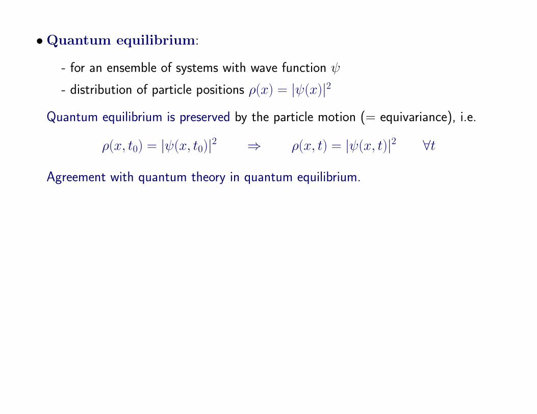
•Quantum equilibrium:
- for an ensemble of systems with wave function ψ
- distribution of particle positions ρ(x) = |ψ(x)|2
Quantum equilibrium is preserved by the particle motion (= equivariance), i.e.
ρ(x, t0) = |ψ(x, t0)|2 ⇒ ρ(x, t) = |ψ(x, t)|2 ∀t
Agreement with quantum theory in quantum equilibrium.
5

• Effective collapse of the wave function
– Branching of the wave function: ψ → ψ1 + ψ2 ψ1ψ2 = 0
– Effective collapse ψ → ψ1 (ψ2 does no longer effect the motion of the config-
uration X)
6
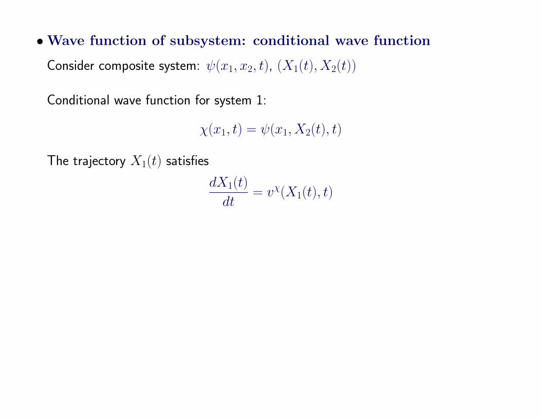
•Wave function of subsystem: conditional wave function
Consider composite system: ψ(x1, x2, t), (X1(t), X2(t))
Conditional wave function for system 1:
χ(x1, t) = ψ(x1, X2(t), t)
The trajectory X1(t) satisfies
dX1(t)
dt= vχ(X1(t), t)
7

•Wave function of subsystem: conditional wave function
Consider composite system: ψ(x1, x2, t), (X1(t), X2(t))
Conditional wave function for system 1:
χ(x1, t) = ψ(x1, X2(t), t)
The trajectory X1(t) satisfies
dX1(t)
dt= vχ(X1(t), t)
Collapse of the conditional wave function
Consider measurement:
– Wave function system: ψ(x) =∑
i ciψi
(ψi are the eigenstates of the operator that is measured)
– Wave function measurement device: φ(y)
– During measurement:
Total wave function: ψ(x)φ(y)→∑
i ciψi(x)φi(y)
Conditional wave function: ψ(x)→ ψi(x)
8
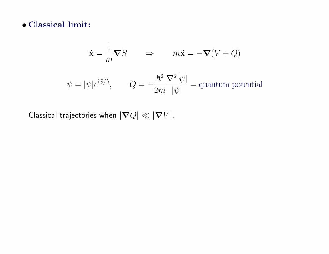
•Classical limit:
x =1
m∇S ⇒ mx = −∇(V + Q)
ψ = |ψ|eiS/~, Q = − ~2
2m
∇2|ψ||ψ|
= quantum potential
Classical trajectories when |∇Q| |∇V |.
9

•Non-locality:
dXk(t)
dt= vψtk (X1(t), . . . , XN(t))
→ Velocity of one particle at a time t depends on the positions of all the other
particles at that time, no matter how far they are.
10
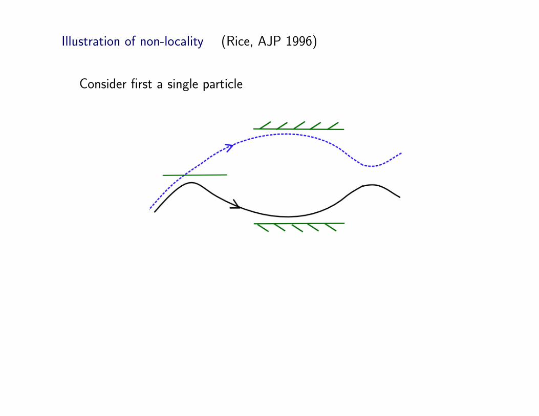
Illustration of non-locality (Rice, AJP 1996)
Consider first a single particle
11

Illustration of non-locality (Rice, AJP 1996)
Consider the entangled state | 〉| 〉 + | 〉| 〉
12
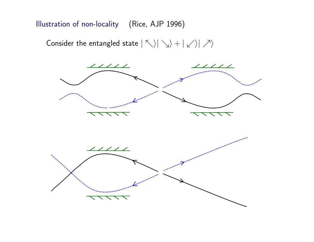
Illustration of non-locality (Rice, AJP 1996)
Consider the entangled state | 〉| 〉 + | 〉| 〉
13

Illustration of non-locality (Rice, AJP 1996)
Consider the entangled state | 〉| 〉 + | 〉| 〉
Non-local, but no faster than light signalling!
14

• Extensions to quantum field theory
– Two natural possible ontologies: particles and fields. Particles seem to work
better for fermions, fields for bosons.
– Example: scalar field
Hamiltonian:
H =1
2
∫d3x
(Π2 + (∇φ)2 + m2φ2
), [φ(x), Π(y)] = iδ(x− y)
Functional Schrodinger representation:
φ(x)→ φ(x) , π(x)→ −iδ
δφ(x)
i∂Ψ(φ, t)
∂t=
1
2
∫d3x
(− δ2
δφ2+ (∇φ)2 + m2φ2
)Ψ(φ, t) .
Bohmian field φ(x) with guidance equation:
∂φ(x, t)
∂t=δS(φ, t)
δφ(x)
∣∣∣φ=φ(x,t)
, Ψ = |Ψ|eiS
Similarly for other bosonic fields (see Struyve (2010) for a review):
electromagnetic field: Ψ(A), A(x), gravity: Ψ(g), g(x), . . .
15
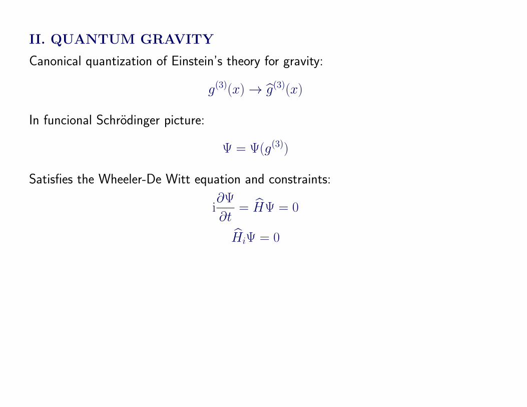
II. QUANTUM GRAVITY
Canonical quantization of Einstein’s theory for gravity:
g(3)(x)→ g(3)(x)
In funcional Schrodinger picture:
Ψ = Ψ(g(3))
Satisfies the Wheeler-De Witt equation and constraints:
i∂Ψ
∂t= HΨ = 0
HiΨ = 0
16

II. QUANTUM GRAVITY
Canonical quantization of Einstein’s theory for gravity:
g(3)(x)→ g(3)(x)
In funcional Schrodinger picture:
Ψ = Ψ(g(3))
Satisfies the Wheeler-De Witt equation and constraints:
i∂Ψ
∂t= HΨ = 0
HiΨ = 0
Conceptual problems:
1. Problem of time: There is no time evolution, the wave function is static.
(How can we tell the universe is expanding or contracting?)
2. Measurement problem: We are considering the whole universe. There are no
outside observers or measurement devices.
3. What is the meaning of space-time diffeomorphism invariance? (The constraints
HiΨ = 0 only express invariance under spatial diffeomorphisms.)
17

Bohmain approach
In a Bohmian approach we have an actual 3-metric g(3) which satisfies:
g(3) = vΨ(g(3))
This solves problems 1:
- We can tell whether the universe is expanding or not, whether it goes into a
singularity or not, etc.
- We can derive time dependent Schrodinger equation for conditional wave function.
E.g. suppose gravity and scalar field. Conditional wave functional for scalar field
Ψs(φ, t) = Ψ(φ, g(3)(t))
is time-dependent if g(3)(t) is time-dependent.
It also solves problem 2. Does it solve problem 3?
For more details, see: Goldstein & Teufel, Callender & Weingard, Pinto-Neto, . . .
18

III. SEMI-CLASSICAL GRAVITY
Apart from the conceptual difficulties with the quantum treatment of gravity, there
are also technical problems: finding solutions to Wheeler-DeWitt equation, doing
perturbation theory, etc. Therefore one often resorts to semi-classical approximations:
→Matter is treated quantum mechanically, as quantum field on curved
space-time.
E.g. scalar field:
i∂tΨ(φ, t) = H(φ, g)Ψ(φ, t)
→Grativity is treated classically, described by
Gµν(g) =8πG
c4〈Ψ|Tµν(φ, g)|Ψ〉
Gµν = Rµν −1
2Rgµν
19

Is there a better semi-classical approximation based on Bohmian
mechanics?
In Bohmian mechanics matter is described by Ψ(φ) and actual scalar field φB(x, t).
Proposal for semi-classical theory:
Gµν(g) =8πG
c4Tµν(φB, g)
20

Is there a better semi-classical approximation based on Bohmian
mechanics?
In Bohmian mechanics matter is described by Ψ(φ) and actual scalar field φB(x, t).
Proposal for semi-classical theory:
Gµν =8πG
c4Tµν(φB)
→ In general doesn’t work because ∇µTµν(φB) 6= 0!
(In non-relativistic Bohmian mechanics energy is not conserved.)
21

Is there a better semi-classical approximation based on Bohmian
mechanics?
In Bohmian mechanics matter is described by Ψ(φ) and actual scalar field φB(x, t).
Proposal for semi-classical theory:
Gµν =8πG
c4Tµν(φB)
→ In general doesn’t work because ∇µTµν(φB) 6= 0!
(In non-relativistic Bohmian mechanics energy is not conserved.)
Similar situation in scalar electrodynamics:
Quantum matter field described by Ψ(φ) and actual scalar field φB(x, t). Semi-
classical theory:
∂µFµν = jν(φB)
→ In general doesn’t work because ∂νjν(φB) 6= 0!
22

Semi-classical approximation to non-relativistic quantum mechanics
• System 1: quantum mechanical. System 2: classical
Usual approach (mean field):
i∂tψ(x1, t) =
(− ∇
21
2m1+ V (x1, X2(t))
)ψ(x1, t)
m2X2(t) = 〈ψ|F2(x1, X2(t))|ψ〉 =
∫dx1|ψ(x1, t)|2F2(x1, X2(t)) , F2 = −∇2V
→ backreaction through mean force
23

Semi-classical approximation to non-relativistic quantum mechanics
• System 1: quantum mechanical. System 2: classical
Usual approach (mean field):
i∂tψ(x1, t) =
(− ∇
21
2m1+ V (x1, X2(t))
)ψ(x1, t)
m2X2(t) = 〈ψ|F2(x1, X2(t))|ψ〉 =
∫dx1|ψ(x1, t)|2F2(x1, X2(t)) , F2 = −∇2V
→ backreaction through mean force
Bohmian approach:
i∂tψ(x1, t) =
(− ∇
21
2m1+ V (x1, X2(t))
)ψ(x1, t)
X1(t) = vψ1 (X1(t), t) , m2X2(t) = F2(X1(t), X2(t))
→ backreaction through Bohmian particle
24

• Prezhdo and Brookby (2001):
Bohmian approach yields better results than usual approach:
25

•Derivation of Bohmian semi-classical approximation
Full quantum mechanical description:
i∂tψ(x1, x2, t) =
(− ∇
21
2m1− ∇
22
2m2+ V (x1, x2)
)ψ(x1, x2, t)
X1(t) = vψ1 (X1(t), X2(t), t) , X2(t) = vψ2 (X1(t), X2(t), t)
Conditional wave function χ(x1, t) = ψ(x1, X2(t), t) satisfies
i∂tχ(x1, t) =
(− ∇
21
2m1+ V (x1, X2(t))
)χ(x1, t) + I(x1, t)
and particle two:
m2X2(t) = −∇2V (X1(t), x2)∣∣∣x2=X2(t)
−∇2Q(X1(t), x2)∣∣∣x2=X2(t)
→ Semi-classical approximation follows when I and −∇2Q are negligible
(e.g. when particle 2 is much heavier than particle 1)
26

Bohmian semi-classical approximation to scalar quantum electrody-
namics
Schrodinger equation for matter:
i∂tΨ(φ, t) = H(φ,A)Ψ(φ, t)
Guidance equation
φ = vΨ(φ, t)
Classical Maxwell equations for with quantum correction:
∂µFµν = jν+jνQ ,
Is consistent since: ∂µ(jµ + jµQ) = 0.
→Crucial in the derivation was that gauge was eliminated!
How to eliminate it in canonical quantum gravity?
(in this case: gauge = spatial diffeomorphism invariance).
27

Bohmian semi-classical approximation to mini-superspace model
• Restriction to homogeneous and isotropic (FLRW) metrics and fields:
– Gravity: ds2 = dt2 − a(t)2dΩ23
– Matter: φ = φ(t)
Wheeler-DeWitt equation:
(HG + HM)ψ = 0 ,
HG =1
4a2∂a(a∂a) + a3VG , HM = − 1
2a3∂2φ + a3VM
Guidance equations:
a = − 1
2a∂aS , φ =
1
a3∂φS
• Semi-classical approximation:
i∂tψ = HMψ , φ =1
a3∂φS
and Friedmann equation with quantum correction:
a2
a2=φ2
2+ VM + VG+Q
28

IV. QUANTUM-TO-CLASSICAL TRANSITION IN INFLATION
THEORY
Cosmological perturbations
Inflaton field: ϕ(x, η) = ϕ0(η) + δϕ(x, η)
Metric with scalar perturbations, in the longitudinal gauge:
ds2 = a2(η)
[1 + 2φ(η,x)] dη2 − [1− 2φ(η,x)] δijdxidxj
,
Gauge invariant Mukhanov-Sasaki variable which describes perturbations:
y ≡ a
[δϕ +
ϕ′0Hφ
],
with H = a′
a the comoving Hubble parameter. Its classical equation of motion is:
y′′ −∇2y − z′′
zy = 0 (z = aϕ′0/H)
So we have 3 variables: a, ϕ0 and y.
– a and ϕ0 are treated classically and independent of y
– y is quantized. The assumed quantum state Ψ(y) is the Bunch-Davies vacuum.
29

The quantum vacuum fluctuations give rise to
the fluctuations in CMB
to structures such as galaxies, clusters of galaxies, etc.
30

The quantum vacuum fluctuations give rise to
the fluctuations in CMB
to structures such as galaxies, clusters of galaxies, etc.
However:
→ How does the vacuum state of the perturbations, which is homogeneous and
isotropic, gives rise to perturbations which are inhomogeneous and anisotropic?
→ How do the quantum fluctuations become classical fluctuations?
31

According to standard quantum theory this can only be achieved by collapse of the
wave function. But collapse is supposed to happen upon measurement. But when
exactly does a measurement happen? Which processes count as measurements in
the early universe?
→Measurement problem!
32

According to standard quantum theory this can only be achieved by collapse of the
wave function. But collapse is supposed to happen upon measurement. But when
exactly does a measurement happen? Which processes count as measurements in
the early universe?
→Measurement problem!
Possible solutions:
collapse theories (Sudarsky), many worlds, Bohmian mechanics
33

According to standard quantum theory this can only be achieved by collapse of the
wave function. But collapse is supposed to happen upon measurement. But when
exactly does a measurement happen?
→Measurement problem
→ Is especially severe in cosmological context! Which processes count as measure-
ment in the early universe?
Possible solutions:
collapse theories (Sudarsky), many worlds, Bohmian mechanics
→ We illustrate the problem and possible solutions in the simple cases of
a decaying atom
the inverted harmonic oscillator
(For Bohmian treatment of the problem in inflation theory, see Pinto-Neto, Santos,
Struyve 2012)
34
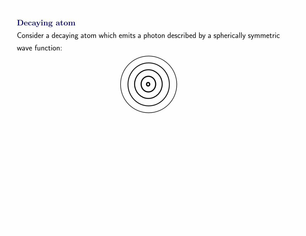
Decaying atom
Consider a decaying atom which emits a photon described by a spherically symmetric
wave function:
35
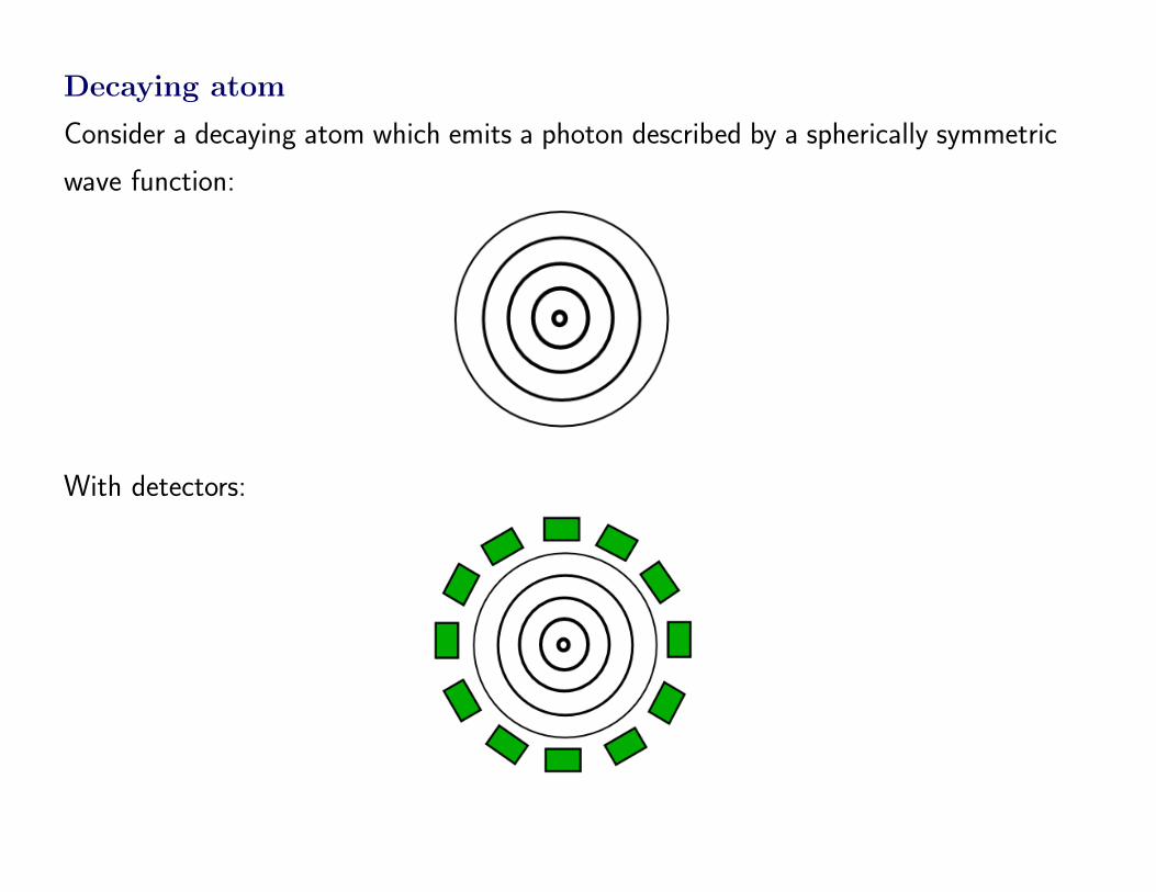
Decaying atom
Consider a decaying atom which emits a photon described by a spherically symmetric
wave function:
With detectors:
36

Decaying atom
Consider a decaying atom which emits a photon described by a spherically symmetric
wave function:
With detectors:
→ according to standard quantum theory collapse breaks the symmetry
37

Bohmian description:
Without detectors:
With detectors:
→ actual particle breaks the symmetry
38

Inverted harmonic oscillator (e.g. Albrecht et al. 1994)
Classical treatment
Potential: V = −q2
2
Equation of motion: q = q
Possible trajectories: q = Aet + Be−t
39

Inverted harmonic oscillator (e.g. Albrecht et al. 1994)
Classical treatment
Potential: V = −q2
2
Equation of motion: q = q
Possible trajectories: q = Aet + Be−t
In phase space:
q = Aet + Be−t, p = Aet −Be−t
q ≈ p ≈ Aet for t 1
⇒ squeezing
40

Quantum mechanics
Squeezed state:
ψ(q, t) = N exp
(− (B − iC)
2q2 − i
B
2t
)
N =
(B
π
)14
, B =1
cosh 2t, C = tanh 2t
Note
∆q2 =1
2B, ∆p2 =
B
2+C2
2B
For t = 0 : ∆q2 = ∆p2 =1
2For t 1 : ∆q2 ≈ ∆p2 1
→ Initially minimum uncertainty in q and p. However, both spread in time!
→ The wave function is not peaked around a classical trajectory!
How can it correspond to a classical system?
41

Common classicality arguments
1. Commuting observables
Heisenberg operators (time evolution O(t) = eiHtO(0)e−iHt):
q(t) = Aet + Be−t , p(t) = Aet − Be−t
(with A = 12 (q(0) + p(0)), B = 1
2 (q(0)− p(0)))
For t 1:
q(t) ≈ p(t) ≈ Aet
Hence
[q(t), p(t)] ≈ 0 ⇒ Classicality
42

Common classicality arguments
1. Commuting observables
Heisenberg operators (time evolution O(t) = eiHtO(0)e−iHt):
q(t) = Aet + Be−t , p(t) = Aet − Be−t
(with A = 12 (q(0) + p(0)), B = 1
2 (q(0)− p(0)))
For t 1:
q(t) ≈ p(t) ≈ Aet
Hence
[q(t), p(t)] ≈ 0 ⇒ Classicality
However
[q(t), p(t)] = i /≈ 0
43
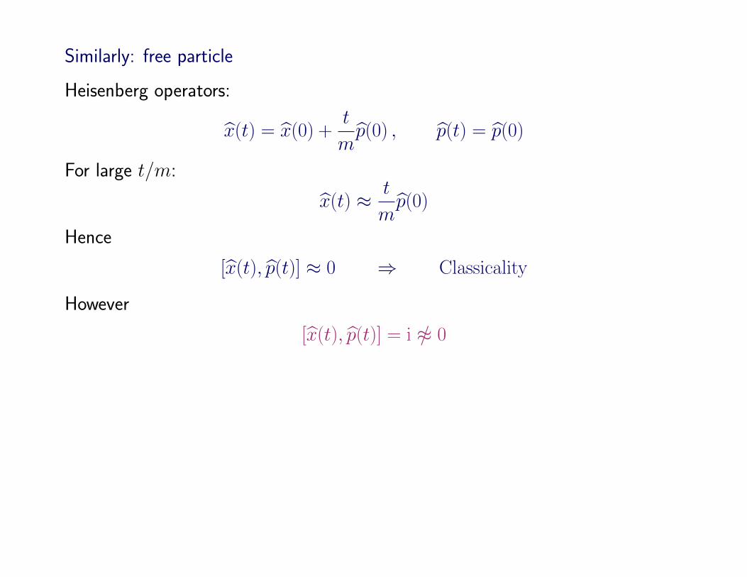
Similarly: free particle
Heisenberg operators:
x(t) = x(0) +t
mp(0) , p(t) = p(0)
For large t/m:
x(t) ≈ t
mp(0)
Hence
[x(t), p(t)] ≈ 0 ⇒ Classicality
However
[x(t), p(t)] = i /≈ 0
44

Similarly: free particle
Heisenberg operators:
x(t) = x(0) +t
mp(0) , p(t) = p(0)
For large t/m:
x(t) ≈ t
mp(0)
Hence
[x(t), p(t)] ≈ 0 ⇒ Classicality
However
[x(t), p(t)] = i /≈ 0
A correct argument:
∆x(t)2 = ∆x(0)2 +t
m
(〈x(0), p(0)〉 − 〈x(0)〉〈p(0)〉
)+t2
m2∆p(0)2
≈ ∆x(0)2 for smallt
m
⇒ No spreading for a very massive particle for short enough times.
45

2. Wigner distribution:
ρ(q, p, t) =1√πB|ψ(q, t)|2 exp
(− (p− Cq)2
B
)→ |ψ(q, t)|2δ(p− q) for t 1
→ Is not peaked around one particular classical trajectory
→ But:
- is positive (is usually not the case)
- satisfies Liouville equation dρ/dt = 0 (is usually not the case)
- quantum mechanical expectation values equal classical averages over ρ
However, this does not mean classical limit is achieved!
46

3. WKB limit
With ψ = |ψ|eiS:∂S
∂t+
(∇S)2
2+ V + Q = 0 ,
V = −q2
2, Q =
B
2(1−Bq2)
For t 1:∂S
∂t+
(∇S)2
2+ V ≈ 0 ,
→ Formally same as classical Hamilton-Jacobi equation
But:
Does not imply we can assume a classical trajectory
47

4. Decoherence
Decoherence due to coupling with other degrees of freedom may yield decompo-
sition of ψ into “classical wave packets”. Collapse may select one of these.
Where does the decoherence come from in inflation theory?
– Interactions between sub and super Hubble modes (which would show up when
treating the fluctuations up to second order).
– Interactions with the matter fields
48

De Broglie-Bohm description description of the inverted oscillator
q = ∇S ⇒ q = FC + FQ
Classical force: FC = q
Quantum force: FQ = qB2
Ratio:FQFC
= B2 → 0 for t 1 → classical behaviour
More precisely:
q(t) ∼√
e2t + e−2t
∼ et for t 1
→ No appeal to decoherence!
→ If there is decoherence of the expected type, then this will not affect the clas-
sicality.
49


![Relativistic Bohmian Mechanics - arXivDespite these problems, e orts have been made to generalize relativistic Bohmian mechanics and some of these e orts have been partially successful[[16],[18]-[22]]](https://static.fdocuments.net/doc/165x107/5e9f90eb2a56356c6243dda2/relativistic-bohmian-mechanics-arxiv-despite-these-problems-e-orts-have-been.jpg)


