Casey Anderson, Paige Leishman, and Joan Wang

Economics 312

May 5, 2012

The effect of incarceration on unemployment in the United States

Abstract:

This paper examines the relationship between prisoner incarceration in the United States and the rate of unemployment. Using state panel data we construct a fixed effects model of unemployment that incorporates a comprehensive range of macroeconomic variables with a focus on state unemployment rates, prison populations, and crime rates. First, we find that growth in prison incarceration rates drastically reduces unemployment. Next, concerned with potential endogeneity between unemployment and prison population we construct vector auto regression models for a representative selection of states and find significant causation both directions between prison population and unemployment. We then attempt to correct for endogeneity with a fixed effect 2SLS regression but cannot find strong instruments.

Introduction:

The prison as it exists in modern times is a relatively novel invention that traces its history back to the mid nineteen hundreds and the utilitarian social philosophy of Jeremy Bentham. The ideal prison in Bentham’s mind was exemplary of the panopticon, institutions were the observers are unobservable and the observed police themselves due to the constant threat of observation. In Bentham’s mind panoptic institutions maximized the effectiveness of the reformation process by forcing introspection and conformation while minimizing and offsetting expenditures by using a skeleton staff and prison labor.

Since the early 1980’s no country has more readily embraced mass incarceration than the United States. More than one in every one hundred American males eighteen years or older reside in prison. The combined male and female imprisonment rate in the US is 500 per 100,000 inhabitants as of 2011. In contrast in the UK 152 people in every 100,000 inhabitants are imprisoned in any given year. In China as of 2007 119 people out of every 100,000 inhabitants were imprisoned. The average rate of imprisonment by EU members stands at 129 per 100,000 inhabitants.

Further, historically the US has experienced consistently lower unemployment rates than those experienced by European economies. However, structurally the explanation for the unemployment gap is far from clear. The EU and US similar economic and policy institutions along with similar

industry compositions and similar levels of output, 47,000 international dollars per capita in the US and 31,000 international dollars per capita in the EU.

One potential explanation for this difference is that prisoners are not counted by official unemployment statistics and higher imprisonment in the US masks unemployment. Evidence for this claim has been produced by converting the difference between the US and EU prison populations into unemployed. This yield the following equation 500 – 129 = 371 prisoners per 100,000 in the US greater than the EU, then 371/500 = 0.742 the percent difference, 0.742*1,612,395 = 1196397 difference in total prison populations. Next we add this to the current number of unemployed 14726400 + 1196397 = 15922797. Then 15922797/153400000 gives the adjusted unemployment rate of 10.4% or an increase of 0.8%. This indicates that the US may be concealing unemployment through increased prison populations.

This project addresses the concern that unemployment in the US may be artificially low due to an interaction effect with prison populations. Due to gendered nature of the US corrections system, male inmate outnumber female inmates more than ten to one, we chose to look at only male corrections. We use panel data analysis across the 48 continental United States between the years 1967 and 2010 to model the unemployment rate with various correction and crime variables included. After correcting for non-stationary variables we find a statistically significant effect of -1.735 on the unemployment rate for every percent the growth of incarceration increases. This finding supports the idea that the US could pursue a policy of mass incarceration to reduce unemployment.

However, if the US were to pursue mass incarceration to reduce unemployment it would imply endogeneity between unemployment and prison population. Imprisonment directly lowers the number of individuals in the labor force and thus the unemployment rate as either the prisoners were unemployed or leave a job opening to be filled. Policies that broaden or harshen sentencing in such a way to increase prison growth rates will also lower unemployment rates. Further, policy setters are incentivized to lower unemployment rates to signal positive economic policy and increase their odds of reelection. Hence, if one were to find endogeneity between prison population and unemployment it would suggest that the US does artificially lower unemployment using mass incarceration.

We proceed to use a simple vector autoregressive model to determine potential endogeneity between the unemployment rate and the growth of prison population rate. We choose to use a standard VAR model to look at representative states. For each state we find statistically significant granger causation in both directions between prison population growth rate and the unemployment rate. However, we are unable to definitely determine an effect.

After the VAR models suggested endogenity we attempted to use an IV 2SLS model to correct for endogineity. However, our instrumental variables were not strong.

Data and Collection Methodology

This paper utilized a balanced panel data set that contains a diverse range of variables for the 48 continental States across a varying number of years from a variety of different sources.

Expenditure data was compiled from the Annual Survey of State and Local Government Finances conducted by the United States Census Bureau. The expenditure dataset is in nominal US dollars as reported by state and local agencies to the US Census Bureau from 1967 to 2010 for the 48 continental United States.

For state-by-state crime statistics we used the Uniform Crime Reporting Statistics dataset compiled annually by the Federal Bureau of Investigation using self-reported crime statistics from state and local agencies which are representative of 94.6% of the US population.

We used the Annual Parole Survey conducted by the Bureau of Justice Statistics (BJS) contains state-by-state data on number of parolees as reported by parole agencies from 1977 to 2010. We omitted female parolees from the dataset due to the small sample size.

The total number of prisoners by state was compiled by the BJS in the National Prisoner Statistics Survey, which surveys local, state and federal corrections facilities. The sample runs from 1978 to 2010.

Data on unionization was collected for the Current Population Survey conducted jointly by the Census Bureau and the U.S. Bureau of labor Statistics (BLS). The dataset contains state-by-state observations from 1984 to 2010.

State-by-state CPI rates were collected from the economic report of the president from 1977 to 2010.

Minimum wage data by state was compiled by the BLS from 1968 to 1999 using data from the Book of the States, 1968-1999 edition, and from 2000 to 2010 using data provided by the U.S. Department of Labor.

A datset on unemployment benefits, average weekly wage, and average duration of unemployment was procured from the Department of Labors Unemployment Insurance Financial Data Handbook (ET Financial Data Handbook 397), which contains observations by state from 1968 to 2010.

Further data on population demographics was acquired from Reed College economics professor Jon Rork.

Dataset Definitions and Summaries

Stfips – State id code that runs from 1 to 48 alphabetically by continental State

Year – year of sample collection from 1967 to 2010

Crime Rates – all crime rates are reported in incidents per 100,000 inhabitants, denoted by the suffix rate

Violent crime - murder and nonnegligent manslaughter, forcible rape, robbery, and aggravated assault.

Murder and nonnegligent manslaughter - The willful (non-negligent) killing of one human being by another.

Forcible rape - The carnal knowledge of a female forcibly and against her will. Rapes by force and attempts or assaults to rape, regardless of the age of the victim, are included. Statutory offenses (no force used—victim under age of consent) are excluded.

Robbery - The taking or attempting to take anything of value from the care, custody, or control of a person or persons by force or threat of force or violence and/or by putting the victim in fear.

Aggravated Assault - An unlawful attack by one person upon another for the purpose of inflicting severe or aggravated bodily injury. This type of assault usually is accompanied by the use of a weapon or by means likely to produce death or great bodily harm. Simple assaults are excluded.

Property Crime Total - Burglary, larceny-theft, motor vehicle theft, and arson. The object of the theft-type offenses is the taking of money or property, but there is no force or threat of force against the victims. The property crime category includes arson because the offense involves the destruction of property; however, arson victims may be subjected to force.

Burglary - The unlawful entry of a structure to commit a felony or a theft. Attempted forcible entry is included.

Larceny-theft - The unlawful taking, carrying, leading, or riding away of property from the possession or constructive possession of another. Examples are thefts of bicycles, motor vehicle parts and accessories, shoplifting, pocketpicking, or the stealing of any property or article that is not taken by force and violence or by fraud. Attempted larcenies are included. Embezzlement, confidence games, forgery, check fraud, etc., are excluded.

Motor Vehicle Theft - The theft or attempted theft of a motor vehicle. A motor vehicle is self-propelled and runs on land surface and not on rails. Motorboats, construction equipment, airplanes, and farming equipment are specifically excluded from this category.

Adults on probation – Total number of male adults on probation

Prisoner Population – Male’s incarcerated in local jails and state or federal prisons.

Education – Expenditure on schools, colleges, and other educational institutions (e.g., for blind, deaf, and other handicapped individuals), and educational programs for adults, veterans, and other special classes. State institutions of higher education includes activities of institutions operated by the state, except that agricultural extension services and experiment stations are classified under Natural resources and hospitals serving the public are classified under Hospitals. Revenue and expenditure for dormitories, cafeterias, athletic events, bookstores, and other auxiliary enterprises financed mainly through charges for services are reported on a gross basis. Reported in nominal US dollars.

Publicwelfare - Expenditure on support of and assistance to needy persons contingent upon their need. Excludes pensions to former employees and other benefits not contingent on need. Expenditures under this heading include: Cash assistance paid directly to needy persons under the categorical programs (Old Age Assistance, Temporary Assistance for Needy Families (TANF) and under any other welfare programs; Vendor payments made directly to private purveyors for medical care, burials, and other commodities and services provided under welfare programs; and provision and operation by the government of welfare institutions. Other public welfare includes payments to other governments for welfare purposes, amounts for administration, support of private welfare agencies, and other public welfare services. Health and hospital services provided directly by the government through its own hospitals and health agencies, and any payments to other governments for such purposes are classed under those functional headings rather than here. Reported in nominal US dollars.

Hospitals - Expenditure on financing, construction acquisition, maintenance or operation of hospital facilities, provision of hospital care, and support of public or private hospitals. Own hospitals are facilities administered directly by the government concerned; Other hospitals refers to support for hospital services in private hospitals or other governments. However, see welfare concerning vendor payments under welfare programs. Nursing homes are included under Public welfare unless they are directly associated with a government hospital. Reported in nominal US dollars.

Health – Expenditure on outpatient health services, other than hospital care, including: public health administration; research and education; categorical health programs; treatment and immunization clinics; nursing; environmental health activities such as air and water pollution control; ambulance service if provided separately from fire protection services, and other general public health activities such as mosquito abatement. School health services provided by health agencies (rather than school agencies) are included here. Sewage treatment operations are classified separately. Reported in nominal US dollars.

Police – Expenditure on police departments. Reported in nominal US dollars.

Correction – Expenditure on local and state jails and prions. Reported in nominal US dollars.

Just – Expenditure on courts and activities associated with courts including law libraries, prosecutorial and defendant programs, probate functions, and juries. Reported in nominal US dollars.

Fedtrans - Amounts received from other governments as fiscal aid in the form of shared revenues and grants-in -aid, as reimbursements for performance of general government functions and specific services for the paying government (e.g., care of prisoners or contractual research), or in lieu of taxes, Excludes amounts received from other governments for sale of property, commodities, and utility services. All intergovernmental revenue is classified as General revenue. Reported in nominal US dollars.

Unionmem – percent of non-agricultural labor force unionized

Medhhinc – Median household income

Pct85 – Percent of population over 85 years of age.

Pctold – Percent of population over 65 years of age.

Pctkid – Percent of population between 5 and 17

Urate – State unemployment rate

StateGSP – Gross state product

Pcthighschool - percent of population holding a GED

Pctcollege – percent of population holding an associates degree or higher

Pop – population by state

Cpi – Consumer Price Index controlled by state

Avgactdurunemp - The average duration of compensable unemployment is the n umber of weeks compensated during the year divided by the number of first payments. It may include more than one period of continuous unemployment. It excludes all unemployment for which no benefits were paid, such as waiting periods, disqualifications, and any time after exhaustion of benefits.

Avgweeklywage - The average weekly wage in total reimbursable covered employment is the total wages paid in covered reimbursable employment divided by the quantity of 52 times the average monthly covered employment.

Avgweeklybenefit - The average weekly benefit amount is the benefits paid for total unemployment during the year divided by the number of weeks for which benefits were paid (weeks compensated for total unemployment). Payments for partial unemployment are excluded from both numerator and denominator.

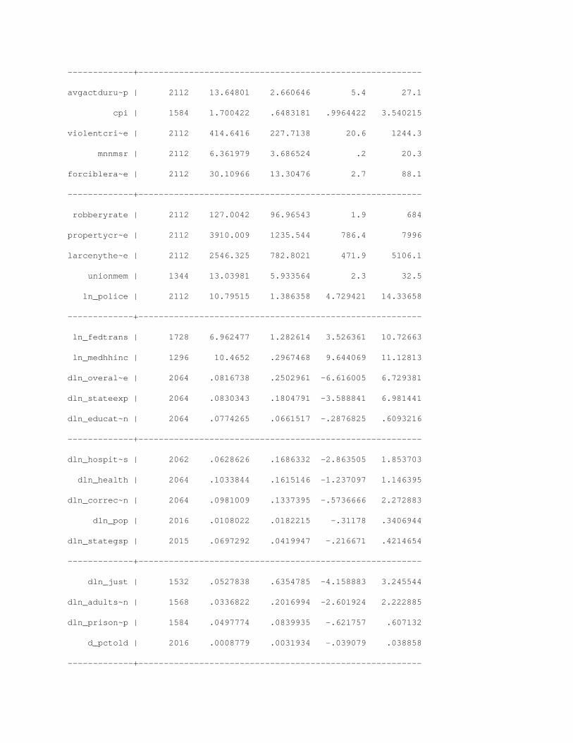
A summary of the transformed data is reproduced below:

Variable | Obs Mean Std. Dev. Min Max

-------------+--------------------------------------------------------

stfips | 2112 24.5 13.85668 1 48

year | 2112 1988.5 12.70143 1967 2010

pct85 | 2064 .0125926 .0046166 .0027 .0284459

urate | 2064 5.681347 2.034393 1.4 18

pcthighsch~l | 1920 72.17151 12.59988 35.2 93

pctcollege | 1920 18.41156 6.505847 2.5 40.4

-------------+--------------------------------------------------------

avgactduru~p | 2112 13.64801 2.660646 5.4 27.1

cpi | 1584 1.700422 .6483181 .9964422 3.540215

violentcri~e | 2112 414.6416 227.7138 20.6 1244.3

mnnmsr | 2112 6.361979 3.686524 .2 20.3

forciblera~e | 2112 30.10966 13.30476 2.7 88.1

-------------+--------------------------------------------------------

robberyrate | 2112 127.0042 96.96543 1.9 684

propertycr~e | 2112 3910.009 1235.544 786.4 7996

larcenythe~e | 2112 2546.325 782.8021 471.9 5106.1

unionmem | 1344 13.03981 5.933564 2.3 32.5

ln_police | 2112 10.79515 1.386358 4.729421 14.33658

-------------+--------------------------------------------------------

ln_fedtrans | 1728 6.962477 1.282614 3.526361 10.72663

ln_medhhinc | 1296 10.4652 .2967468 9.644069 11.12813

dln_overal~e | 2064 .0816738 .2502961 -6.616005 6.729381

dln_stateexp | 2064 .0830343 .1804791 -3.588841 6.981441

dln_educat~n | 2064 .0774265 .0661517 -.2876825 .6093216

-------------+--------------------------------------------------------

dln_hospit~s | 2062 .0628626 .1686332 -2.863505 1.853703

dln_health | 2064 .1033844 .1615146 -1.237097 1.146395

dln_correc~n | 2064 .0981009 .1337395 -.5736666 2.272883

dln_pop | 2016 .0108022 .0182215 -.31178 .3406944

dln_stategsp | 2015 .0697292 .0419947 -.216671 .4214654

-------------+--------------------------------------------------------

dln_just | 1532 .0527838 .6354785 -4.158883 3.245544

dln_adults~n | 1568 .0336822 .2016994 -2.601924 2.222885

dln_prison~p | 1584 .0497774 .0839935 -.621757 .607132

d_pctold | 2016 .0008779 .0031934 -.039079 .038858

-------------+--------------------------------------------------------

d_pctkid | 2016 -.0006302 .0118485 -.0534 .105

d_pcthighs~l | 1824 .9463268 .9730982 -3.199997 4.700005

d_avgweekl~e | 2064 16.46375 10.82907 -75.91003 93.53992

d_avgweekl~t | 2064 5.908973 7.395509 -35.81 76.63998

d_aggravat~e | 2064 3.07093 25.93498 -113.7 172.1

-------------+--------------------------------------------------------

d_burglary~e | 2064 -.3502423 94.87356 -401.2999 575.7

d_motorveh~e | 2064 -1.518023 44.96524 -263 256

dln_minwage | 2016 .0435726 .1038004 -.3184538 1.168993

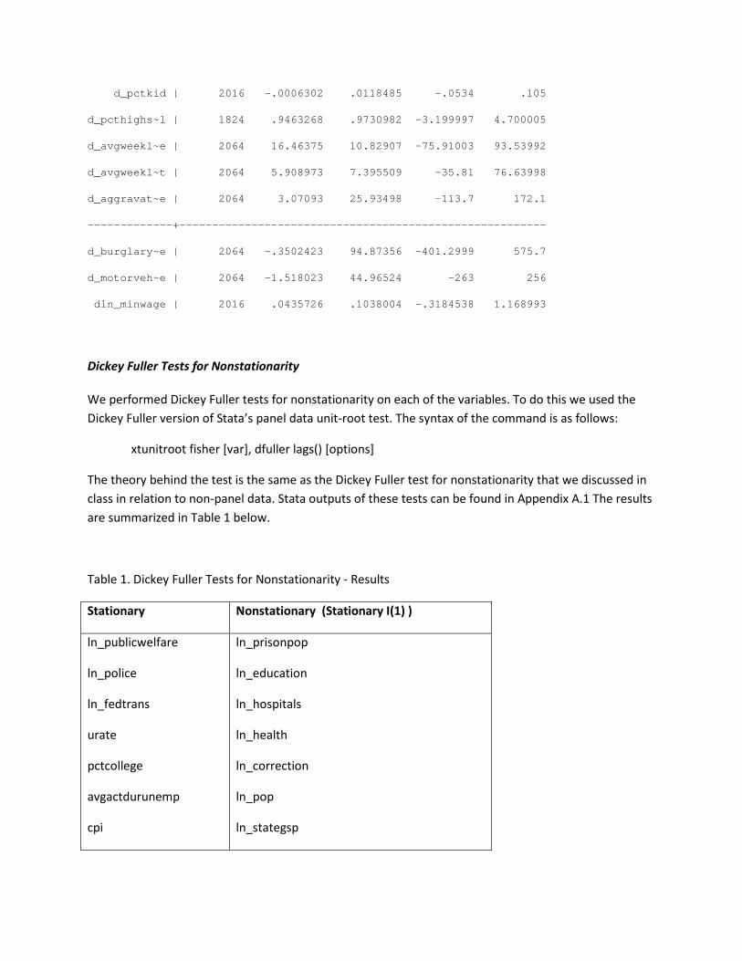
Dickey Fuller Tests for Nonstationarity

We performed Dickey Fuller tests for nonstationarity on each of the variables. To do this we used the Dickey Fuller version of Stata’s panel data unit-root test. The syntax of the command is as follows:

xtunitroot fisher [var], dfuller lags() [options]

The theory behind the test is the same as the Dickey Fuller test for nonstationarity that we discussed in class in relation to non-panel data. Stata outputs of these tests can be found in Appendix A.1 The results are summarized in Table 1 below.

Table 1. Dickey Fuller Tests for Nonstationarity - Results

Stationary Nonstationary (Stationary I(1) )

ln_publicwelfare

ln_police

ln_fedtrans

urate

pctcollege

avgactdurunemp

cpi

ln_prisonpop

ln_education

ln_hospitals

ln_health

ln_correction

ln_pop

ln_stategsp

unionmem

larcenytheftrate

propertycrimerate

robberyrate

forcibleraperate

mnnmsr

violentcrimerate

ln_debt

ln_just

ln_minwage ln_adultsonprobation

pct85

pctold

pctkid

pcthighshool

avgweeklywage

avgweeklybenefit

motorvehicletheftrate

burglaryrate

aggravatedassaultrate

We found all of the nonstationary variables to be integrated of order one. Thus, we used first differenced versions of each of these variables in our regressions.

Fixed Effects vs. Random Effects

In panel data regressions, we use intercept terms to account for individual heterogeneity in states. We want to control for state-specific time-invariant characteristics because we are more interested in looking at the effects of the explanatory variables on the unemployment rate, not so much the effects of the varying state characteristics. There are two ways to account for individual heterogeneity: fixed effects and random effects. Since the “individuals” in our data are states, and all states are included (except for HI, AK, DC), it makes sense that the intercepts that capture individual heterogeneity are “fixed”.

However, there are advantages to treating these state-specific time-invariant characteristics as random. The random effects model saves us more degrees of freedom, which would result in more accurate estimates of the coefficients. It is also capable of estimating the effects of explanatory variables that only vary across states, not time. The only catch is that if there exists correlation between the unobserved difference between states and the existing explanatory variables, then the random effects regression becomes inconsistent. We are going to regress our panel data twice, one with random effects and one with fixed effects. Then, we will use the Hausman test to see if such correlation exists. If so, then we move on to the fixed effects model. In terms of the nature of the unobserved state-specific time-invariant characteristics, it is highly plausible that the omitted time-invariant variables that explain the unemployment rate are correlated with the existing explanatory variables we are using. For example, any related state policies that we didn’t account for would contribute to that correlation. Therefore, we wouldn’t be surprised if we have to use a fixed effects model instead of a random effects model. Note that when we use the Hausman test, Stata does not allow the standard errors in the regression to be robust to heteroskedasticity. However, once we have decided on either random or fixed, we need to use clustering robust standard errors so that we do not need to assume that errors are uncorrelated over time for each state. Below are the Stata commands we used to perform the Hausman test. . quietly xtreg urate dln_education dln_hospitals dln_health dln_correction ln_police dln_pop dln_stategsp dln_just dln_adultsonprobation dln_prisonpop d_pctold d_pctkid d_pct85 d_pcthighschool pctcollege avgactdurunemp d_avgweeklywage d_avgweeklybenefit d_motorvehicletheftrate dln_minwage ln_fedtrans unionmem larcenytheftrate propertycrimerate robberyrate forcibleraperate mnnmsr violentcrimerate d_aggravatedassaultrate d_burglaryrate cpi, fe

. estimates store fe

. quietly xtreg urate dln_education dln_hospitals dln_health dln_correction ln_police dln_pop dln_stategsp dln_just dln_adultsonprobation dln_prisonpop d_pctold d_pctkid d_pct85 d_pcthighschool pctcollege avgactdurunemp d_avgweeklywage d_avgweeklybenefit d_motorvehicletheftrate dln_minwage ln_fedtrans unionmem larcenytheftrate propertycrimerate robberyrate forcibleraperate mnnmsr violentcrimerate d_aggravatedassaultrate d_burglaryrate cpi, re

. estiamtes store re

. hausman fe re

Note: the rank of the differenced variance matrix (20) does not equal the number of

coefficients being tested (31); be sure this is what you expect, or there may be problems computing the test. Examine the output of your estimators for anything unexpected and possibly consider scaling your variables so that the coefficients are on a similar scale.

b = consistent under Ho and Ha; obtained from xtreg

B = inconsistent under Ha, efficient under Ho; obtained from xtreg

Test: Ho: difference in coefficients not systematic

chi2(20) = (b-B)'[(V_b-V_B)^(-1)](b-B)

= 77.27

Prob>chi2 = 0.0000

(V_b-V_B is not positive definite)

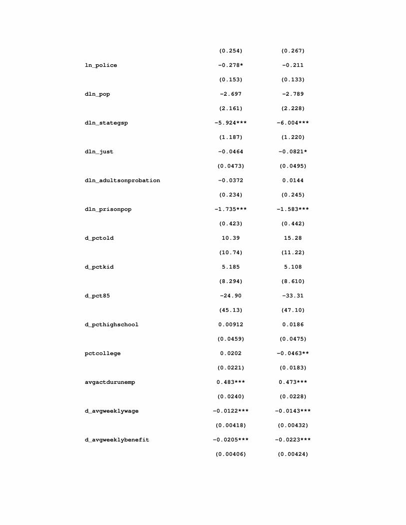
Since the Hausman test gives a chi2 statistic of 77.27, which is bigger than the critical value (20, 0.95) of 31.41, we reject the null hypothesis “corr(u_i, X) = 0” that there exists no correlation between the unobserved difference across states and the existing explanatory variables. Thus, we conclude that we need to use the fixed effects model because the random effects model would create inconsistent estimates. Below is a summary table of the regression results of the two models.

(1)

Fixed Effects

(2)

Random Effects

VARIABLES urate urate

dln_education -0.662 -0.554

(0.484) (0.506)

dln_hospitals -0.548** -0.446*

(0.239) (0.250)

dln_health -0.0131 -0.175

(0.239) (0.250)

dln_correction -0.417 -0.398

(0.254) (0.267)

ln_police -0.278* -0.211

(0.153) (0.133)

dln_pop -2.697 -2.789

(2.161) (2.228)

dln_stategsp -5.924*** -6.004***

(1.187) (1.220)

dln_just -0.0464 -0.0821*

(0.0473) (0.0495)

dln_adultsonprobation -0.0372 0.0144

(0.234) (0.245)

dln_prisonpop -1.735*** -1.583***

(0.423) (0.442)

d_pctold 10.39 15.28

(10.74) (11.22)

d_pctkid 5.185 5.108

(8.294) (8.610)

d_pct85 -24.90 -33.31

(45.13) (47.10)

d_pcthighschool 0.00912 0.0186

(0.0459) (0.0475)

pctcollege 0.0202 -0.0463**

(0.0221) (0.0183)

avgactdurunemp 0.483*** 0.473***

(0.0240) (0.0228)

d_avgweeklywage -0.0122*** -0.0143***

(0.00418) (0.00432)

d_avgweeklybenefit -0.0205*** -0.0223***

(0.00406) (0.00424)

d_motorvehicletheftrate -0.00314*** -0.00340***

(0.000749) (0.000781)

dln_minwage 0.345 0.345

(0.290) (0.303)

ln_fedtrans 0.0382 0.273*

(0.237) (0.158)

unionmem 0.143*** 0.0329**

(0.0254) (0.0168)

larcenytheftrate -0.000974*** -0.000958***

(0.000348) (0.000315)

propertycrimerate 0.000446* 0.000479**

(0.000252) (0.000229)

robberyrate -0.000611 -0.00430***

(0.00164) (0.00144)

forcibleraperate 0.0120** 0.0140***

(0.00548) (0.00518)

mnnmsr 0.0109 0.107***

(0.0301) (0.0273)

violentcrimerate 0.000207 0.000263

(0.000667) (0.000602)

d_aggravatedassaultrate 0.00175 0.00138

(0.00111) (0.00113)

d_burglaryrate 0.000218 0.000193

(0.000444) (0.000464)

cpi 2.408*** 2.765***

(0.459) (0.311)

Constant -3.012 -3.399**

(2.922) (1.437)

Observations 908 908

R-squared (within)

R-squared (between)

R-squared (overall)

0.748

0.1229

0.3664

0.7338

0.4380

0.6073

Number of stfips 48 48

Standard errors in parentheses

*** p<0.01, ** p<0.05, * p<0.1

Analysis of the Preferred Model: the Fixed Effects Model

. xtreg urate dln_education dln_hospitals dln_health dln_correction ln_police dln_pop dln_stategsp dln_just dln_adultsonprobation dln_prisonpop d_pctold d_pctkid d_pct85 d_pcthighschool pctcollege avgactdurunemp d_avgweeklywage d_avgweeklybenefit d_motorvehicletheftrate dln_minwage ln_fedtrans unionmem larcenytheftrate propertycrimerate robberyrate forcibleraperate mnnmsr violentcrimerate d_aggravatedassaultrate d_burglaryrate cpi, fe vce(cluster stfips)

Fixed-effects (within) regression Number of obs = 908

Group variable: stfips Number of groups = 48

R-sq: within = 0.7477 Obs per group: min = 17

between = 0.1229 avg = 18.9

overall = 0.3664 max = 19

F(31,47) = 66.71

corr(u_i, Xb) = -0.5562 Prob > F = 0.0000

(Std. Err. adjusted for 48 clusters in stfips)

-----------------------------------------------------------------------------------------

| Robust

urate | Coef. Std. Err. t P>|t| [95% Conf. Interval]

------------------------+----------------------------------------------------------------

dln_education | -.6615825 .4521723 -1.46 0.150 -1.571236 .2480709

dln_hospitals | -.5483006 .2446897 -2.24 0.030 -1.040553 -.0560484

dln_health | -.0130769 .1913305 -0.07 0.946 -.3979842 .3718304

dln_correction | -.4170741 .209997 -1.99 0.053 -.8395335 .0053853

ln_police | -.277609 .2656034 -1.05 0.301 -.811934 .256716

dln_pop | -2.696942 1.528233 -1.76 0.084 -5.77135 .3774663

dln_stategsp | -5.924324 1.514444 -3.91 0.000 -8.970992 -2.877657

dln_just | -.0464058 .0415328 -1.12 0.270 -.1299589 .0371474

dln_adultsonprobation | -.0372263 .2855898 -0.13 0.897 -.6117588 .5373062

dln_prisonpop | -1.7345 .488286 -3.55 0.001 -2.716805 -.7521955

d_pctold | 10.38621 7.607436 1.37 0.179 -4.917973 25.6904

d_pctkid | 5.18526 7.198255 0.72 0.475 -9.295762 19.66628

d_pct85 | -24.89758 29.72356 -0.84 0.406 -84.69366 34.8985

d_pcthighschool | .0091218 .039362 0.23 0.818 -.0700644 .088308

pctcollege | .0201529 .0264906 0.76 0.451 -.0331392 .073445

avgactdurunemp | .4826801 .0473876 10.19 0.000 .3873484 .5780117

d_avgweeklywage | -.0122453 .0043056 -2.84 0.007 -.0209071 -.0035835

d_avgweeklybenefit | -.0205006 .0046496 -4.41 0.000 -.0298544 -.0111468

d_motorvehicletheftrate | -.0031433 .0009222 -3.41 0.001 -.0049986 -.001288

dln_minwage | .3446052 .3241691 1.06 0.293 -.3075389 .9967493

ln_fedtrans | .0382169 .25483 0.15 0.881 -.4744349 .5508687

unionmem | .1427206 .04343 3.29 0.002 .0553508 .2300904

larcenytheftrate | -.0009745 .0004257 -2.29 0.027 -.0018308 -.0001181

propertycrimerate | .000446 .0003164 1.41 0.165 -.0001904 .0010824

robberyrate | -.0006113 .002563 -0.24 0.813 -.0057673 .0045447

forcibleraperate | .0119852 .0066091 1.81 0.076 -.0013106 .0252811

mnnmsr | .0109469 .0379144 0.29 0.774 -.0653271 .087221

violentcrimerate | .0002067 .0010015 0.21 0.837 -.0018082 .0022215

d_aggravatedassaultrate | .0017531 .0011854 1.48 0.146 -.0006315 .0041377

d_burglaryrate | .0002177 .0004433 0.49 0.626 -.0006741 .0011095

cpi | 2.408425 .5654813 4.26 0.000 1.270823 3.546026

_cons | -3.011854 4.352629 -0.69 0.492 -11.76821 5.744506

------------------------+----------------------------------------------------------------

sigma_u | 1.6304231

sigma_e | .81457717

rho | .80024899 (fraction of variance due to u_i)

-----------------------------------------------------------------------------------------

The variables with statistically significant coefficients at a significance level of 0.05 are highlighted in the regression results table. Note that the constant term, which is the average of the states’ intercepts that measure individual heterogeneity, is insignificant. This tells us that individual heterogeneity is not significantly evident when we are looking at the estimation of unemployment rate. The variable we are most interested in is dln_prisonpop, which is interpreted as the growth rate of the state’s prison population. According to this fixed effects model, a 1% increase in this growth rate would result in an approximately 1.73% decrease in the unemployment rate. This is consistent with our hypothesis in that an explanation for a lower than expected unemployment rate in the US may be attributed to the positive growth rate of prison population. Another statistically significant variable is the gross state product (dln_stategsp). Results show that a $1000 increase in GSP corresponds to a 5.9% decresase in the unemployment rate. This is consistent with macroeconomic theory that higher output leads to more jobs. Furthermore for the variable the average duration of compensable unemployment (avgactdurunemp), if the number of weeks each person received unemployment benefits increased by one week, the unemployment rate would be predicted to increase by 0.48%. This makes sense because there exists a higher incentive to remain unemployed. Another important finding is that if a change in average weekly wage increases by $1, the unemployment rate is expected to decrease by 0.01%. In terms the change in average weekly benefits per person for unemployment, our results show that a $1 increase in benefits is likely to produce a 0.02% decrease in the unemployment rate. This may imply that a higher benefits package leads to more success in finding a job. In addition, the coefficients of the two statistically significant crime-rate variables (motor vehicle theft and larceny) imply a negative effect on the unemployment rate. Thought the coefficients are small, they are consistent with our hypothesis. CPI was included as an indicator of inflation, without it, it is likely that omitted variable would have been a serious issue. Lastly, union membership percentage was found to have a positive effect on the unemployment rate (a 0.14% increase in the unemployment rate). This is likely due to the incentive for unions to attempt to exclude non-unionized workers from the labor force to maximize wages.

Endogeneity, Granger Causality, and Impulse Response

Up until this point, we have assumed that the unemployment rate is the dependent variable. However, we believe that variables like prison population and the unemployment rate might by dynamically interdependent. We want to explore this bivariate system and examine the unique relationship between urate and dln.prisonpop (both stationary) with the vector autoregressive (VAR) model. We decided to pick a few states that “roughly” represent the United States: Texas, Oregon,

Minnesota, New York, California, and Wisconsin. Then, we examine how these two variables behave interdependently in these states with 6 separate VAR models.

For each state, we first use a long lag length (11), which we believed was sufficient to eliminate autocorrelation in the error term. Then, we used the varsoc command in Stata to output several selection-order criteria including AIC and SBIC. In the varsoc tables, we chose the optimal lag length by examining the lag that produces the most desired selection-order criteria values (denoted by *). However, for most of the states we didn’t have enough degrees of freedom to employ the optimal lag length to perform Granger causality tests and IR functions. As a result, we used the lag length that is as close to the optimal lag length as possible while accounted for degrees of freedom.

Since it is difficult to interpret the coefficients of the VAR models directly, we turn to Granger Causality tests and Impulse Response functions to interpret the dynamics of urate and dln.prisonpop. For the Granger Causality test, we use the Stata command “vargranger” to perform several Wald tests. For instance, if we reject the hypothesis that the coefficients on all the lags of the growth rate of prison population are jointly zero, then we conclude that the growth rate of prison population Granger causes the unemployment rate. The Impulse Response functions (IRF) model the contemporaneous effect of a shock in one variable on the other variable. In Stata, we make sure to use the “orthogonalized” IRF plots for the “contemporaneous” effects. Below are the regression and test results for each state followed by analysis.

TEXAS

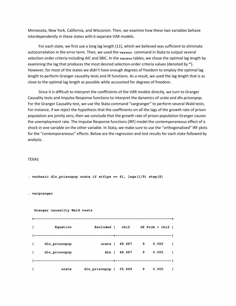
. varbasic dln_prisonpop urate if stfips == 41, lags(1/9) step(8)

. vargranger

Granger causality Wald tests

+------------------------------------------------------------------+

| Equation Excluded | chi2 df Prob > chi2 |

|--------------------------------------+---------------------------|

| dln_prisonpop urate | 48.687 9 0.000 |

| dln_prisonpop ALL | 48.687 9 0.000 |

|--------------------------------------+---------------------------|

| urate dln_prisonpop | 35.669 9 0.000 |

| urate ALL | 35.669 9 0.000 |

+------------------------------------------------------------------+

Test results (3rd row) show that the growth rate of prison population Granger-causes the unemployment rate: given past values of the unemployment rate, past values of the growth rate of prison population are helping for predicting the unemployment rate. Similarly, we can conclude that the unemployment rate Granger-causes the growth rate of prison population (1st row). As a result, there exists Granger-causality between the growth rate of prison population in Texas and the unemployment rate in Texas in both directions.

. irf graph oirf, irf(varbasic) impulse(dln_prisonpop) response(urate)

. irf graph oirf, irf(varbasic) impulse(urate) response(dln_prisonpop)

Figure 1. dln_prisonpop, urate Figure 2. Urate, dln_prisonpop

Figure 1 shows the response of the unemployment rate to a 1% increase in the growth rate of Texas’ prison population. It indicates a slight increase in the unemployment rate between years 2 and 4, after which it decreases and remains below its previous level until year 8. Figure 2, which shows the response of the prison population growth rate to a 1% increase in the unemployment rate, implies a significant increase in the long run.

While the confidence intervals in each graph are encouragingly slim, it is important to note the small unit size on the y-axis. This indicates that the interpretation is certainly statistically significant, but its economic significance is questionable.

The OIRF results for most of the remaining states were generally inconclusive. That is, their confidence intervals tended to include zero at most points. It is possible that this is because we had to use sub-optimal lag lengths as a result of degrees of freedom restrictions.

OREGON

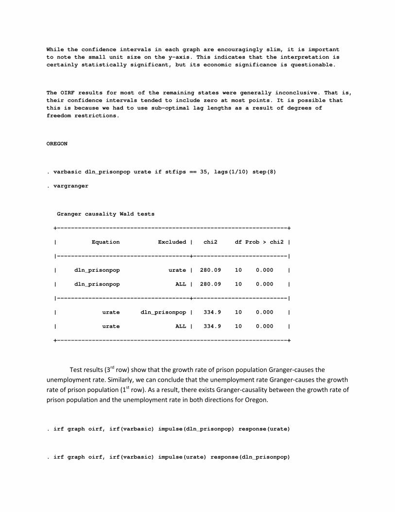
. varbasic dln_prisonpop urate if stfips == 35, lags(1/10) step(8)

. vargranger

Granger causality Wald tests

+------------------------------------------------------------------+

| Equation Excluded | chi2 df Prob > chi2 |

|--------------------------------------+---------------------------|

| dln_prisonpop urate | 280.09 10 0.000 |

| dln_prisonpop ALL | 280.09 10 0.000 |

|--------------------------------------+---------------------------|

| urate dln_prisonpop | 334.9 10 0.000 |

| urate ALL | 334.9 10 0.000 |

+------------------------------------------------------------------+

Test results (3rd row) show that the growth rate of prison population Granger-causes the unemployment rate. Similarly, we can conclude that the unemployment rate Granger-causes the growth rate of prison population (1st row). As a result, there exists Granger-causality between the growth rate of prison population and the unemployment rate in both directions for Oregon.

. irf graph oirf, irf(varbasic) impulse(dln_prisonpop) response(urate)

. irf graph oirf, irf(varbasic) impulse(urate) response(dln_prisonpop)

MINNESOTA

. varbasic urate dln_prisonpop if stfips == 21, lags(1/10) step(8)

. vargranger

Granger causality Wald tests

+------------------------------------------------------------------+

| Equation Excluded | chi2 df Prob > chi2 |

|--------------------------------------+---------------------------|

| urate dln_prisonpop | 2813.8 10 0.000 |

| urate ALL | 2813.8 10 0.000 |

|--------------------------------------+---------------------------|

| dln_prisonpop urate | 105.57 10 0.000 |

| dln_prisonpop ALL | 105.57 10 0.000 |

+------------------------------------------------------------------+

Test results (3rd row) show that the growth rate of prison population Granger-causes the unemployment rate. Similarly, we can conclude that the unemployment rate Granger-causes the growth

rate of prison population (1st row). As a result, there exists Granger-causality between the growth rate of prison population and the unemployment rate in both directions for Minnesota.

. irf graph oirf, irf(varbasic) impulse(dln_prisonpop) response(urate)

. irf graph oirf, irf(varbasic) impulse(urate) response(dln_prisonpop)

NEW YORK

. varbasic dln_prisonpop urate if stfips == 30, lags(1/9) step(8)

. vargranger

Granger causality Wald tests

+------------------------------------------------------------------+

| Equation Excluded | chi2 df Prob > chi2 |

|--------------------------------------+---------------------------|

| dln_prisonpop urate | 39.165 9 0.000 |

| dln_prisonpop ALL | 39.165 9 0.000 |

|--------------------------------------+---------------------------|

| urate dln_prisonpop | 97.83 9 0.000 |

| urate ALL | 97.83 9 0.000 |

+------------------------------------------------------------------+

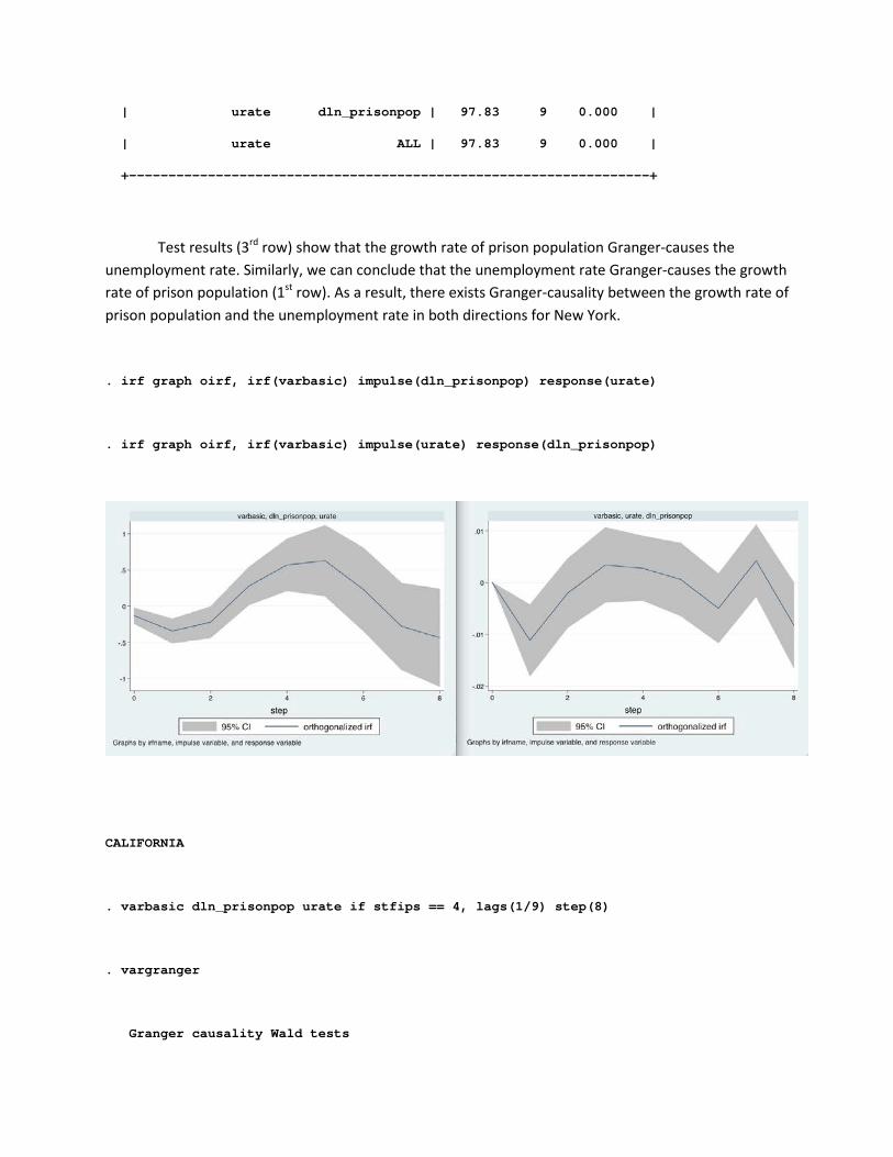
Test results (3rd row) show that the growth rate of prison population Granger-causes the unemployment rate. Similarly, we can conclude that the unemployment rate Granger-causes the growth rate of prison population (1st row). As a result, there exists Granger-causality between the growth rate of prison population and the unemployment rate in both directions for New York.

. irf graph oirf, irf(varbasic) impulse(dln_prisonpop) response(urate)

. irf graph oirf, irf(varbasic) impulse(urate) response(dln_prisonpop)

CALIFORNIA

. varbasic dln_prisonpop urate if stfips == 4, lags(1/9) step(8)

. vargranger

Granger causality Wald tests

+------------------------------------------------------------------+

| Equation Excluded | chi2 df Prob > chi2 |

|--------------------------------------+---------------------------|

| dln_prisonpop urate | 100.39 9 0.000 |

| dln_prisonpop ALL | 100.39 9 0.000 |

|--------------------------------------+---------------------------|

| urate dln_prisonpop | 45.57 9 0.000 |

| urate ALL | 45.57 9 0.000 |

+------------------------------------------------------------------+

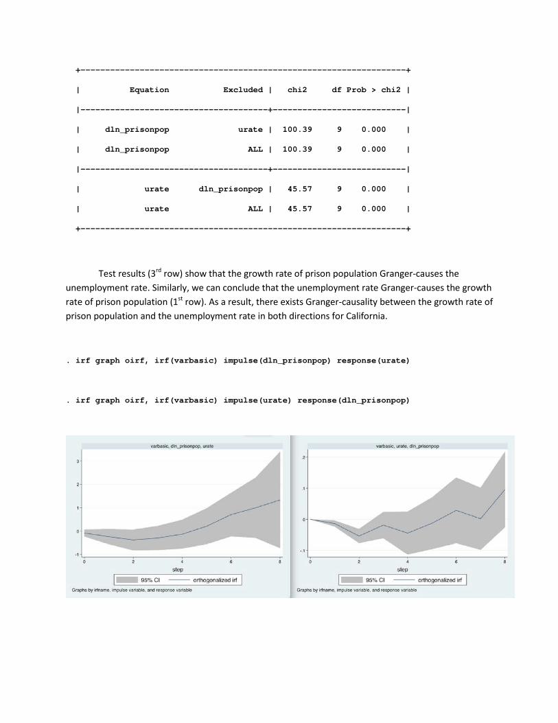
Test results (3rd row) show that the growth rate of prison population Granger-causes the unemployment rate. Similarly, we can conclude that the unemployment rate Granger-causes the growth rate of prison population (1st row). As a result, there exists Granger-causality between the growth rate of prison population and the unemployment rate in both directions for California.

. irf graph oirf, irf(varbasic) impulse(dln_prisonpop) response(urate)

. irf graph oirf, irf(varbasic) impulse(urate) response(dln_prisonpop)

WISCONSIN

. varbasic dln_prisonpop urate if stfips == 47, lags(1/9) step(8)

. vargranger

Granger causality Wald tests

+------------------------------------------------------------------+

| Equation Excluded | chi2 df Prob > chi2 |

|--------------------------------------+---------------------------|

| dln_prisonpop urate | 26.351 9 0.002 |

| dln_prisonpop ALL | 26.351 9 0.002 |

|--------------------------------------+---------------------------|

| urate dln_prisonpop | 55.133 9 0.000 |

| urate ALL | 55.133 9 0.000 |

+------------------------------------------------------------------+

Test results (3rd row) show that the growth rate of prison population Granger-causes the unemployment rate. Similarly, we can conclude that the unemployment rate Granger-causes the growth rate of prison population (1st row). As a result, there exists Granger-causality between the growth rate of prison population and the unemployment rate in both directions for Wisconsin.

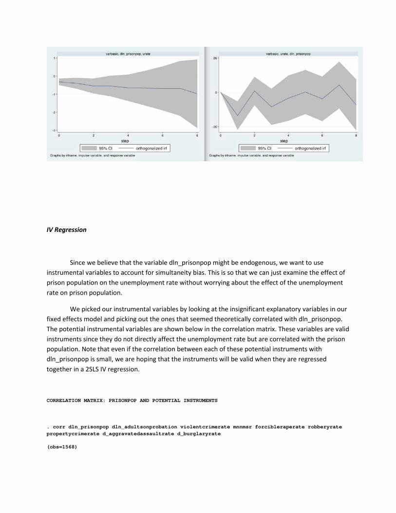
. irf graph oirf, irf(varbasic) impulse(dln_prisonpop) response(urate)

. irf graph oirf, irf(varbasic) impulse(urate) response(dln_prisonpop)

IV Regression

Since we believe that the variable dln_prisonpop might be endogenous, we want to use instrumental variables to account for simultaneity bias. This is so that we can just examine the effect of prison population on the unemployment rate without worrying about the effect of the unemployment rate on prison population.

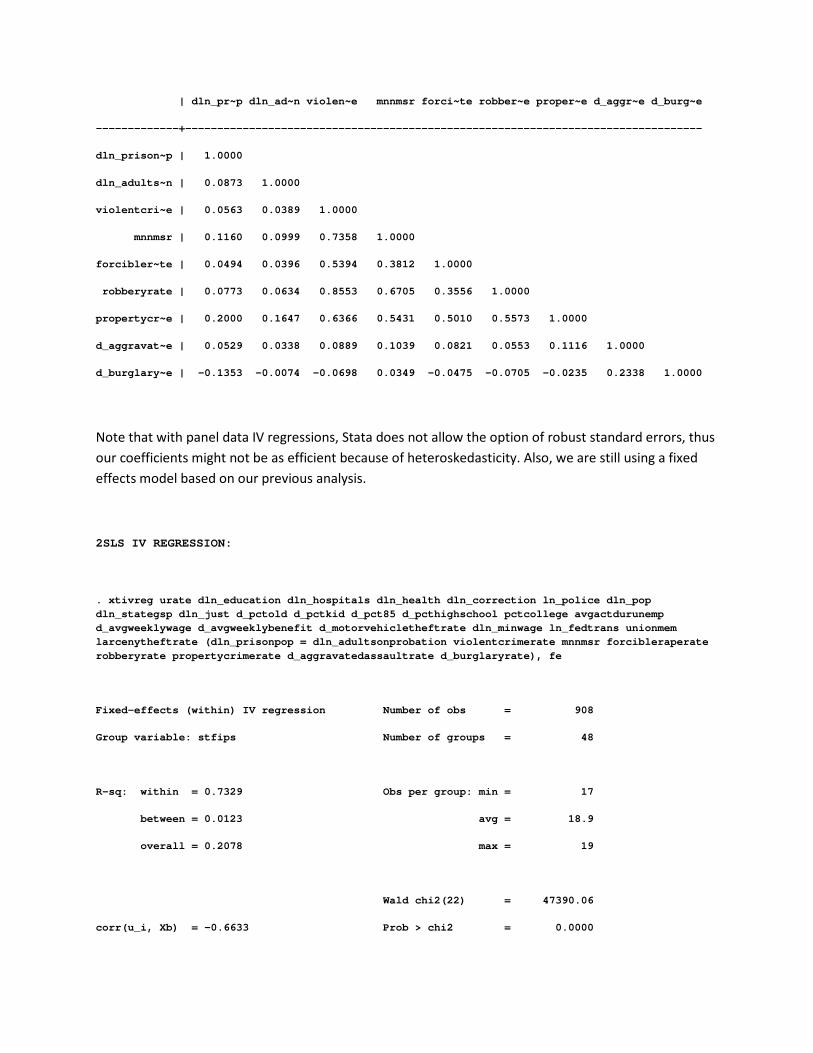
We picked our instrumental variables by looking at the insignificant explanatory variables in our fixed effects model and picking out the ones that seemed theoretically correlated with dln_prisonpop. The potential instrumental variables are shown below in the correlation matrix. These variables are valid instruments since they do not directly affect the unemployment rate but are correlated with the prison population. Note that even if the correlation between each of these potential instruments with dln_prisonpop is small, we are hoping that the instruments will be valid when they are regressed together in a 2SLS IV regression.

CORRELATION MATRIX: PRISONPOP AND POTENTIAL INSTRUMENTS

. corr dln_prisonpop dln_adultsonprobation violentcrimerate mnnmsr forcibleraperate robberyrate propertycrimerate d_aggravatedassaultrate d_burglaryrate

(obs=1568)

| dln_pr~p dln_ad~n violen~e mnnmsr forci~te robber~e proper~e d_aggr~e d_burg~e

-------------+---------------------------------------------------------------------------------

dln_prison~p | 1.0000

dln_adults~n | 0.0873 1.0000

violentcri~e | 0.0563 0.0389 1.0000

mnnmsr | 0.1160 0.0999 0.7358 1.0000

forcibler~te | 0.0494 0.0396 0.5394 0.3812 1.0000

robberyrate | 0.0773 0.0634 0.8553 0.6705 0.3556 1.0000

propertycr~e | 0.2000 0.1647 0.6366 0.5431 0.5010 0.5573 1.0000

d_aggravat~e | 0.0529 0.0338 0.0889 0.1039 0.0821 0.0553 0.1116 1.0000

d_burglary~e | -0.1353 -0.0074 -0.0698 0.0349 -0.0475 -0.0705 -0.0235 0.2338 1.0000

Note that with panel data IV regressions, Stata does not allow the option of robust standard errors, thus our coefficients might not be as efficient because of heteroskedasticity. Also, we are still using a fixed effects model based on our previous analysis.

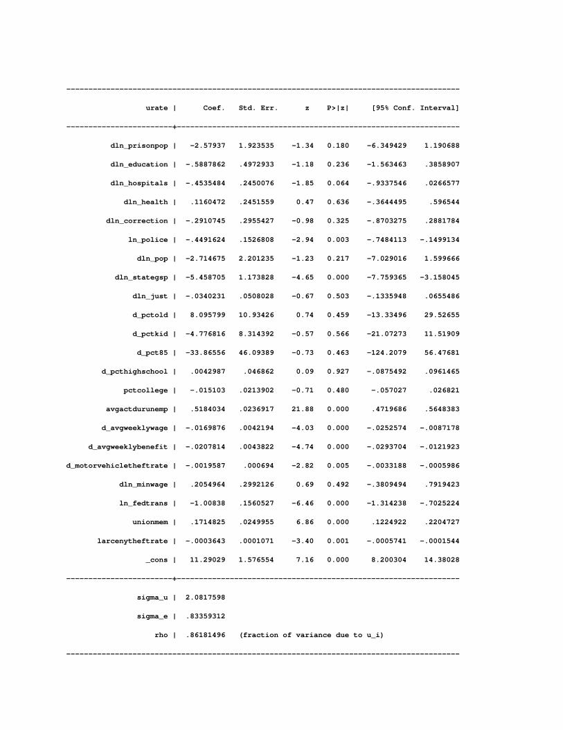
2SLS IV REGRESSION:

. xtivreg urate dln_education dln_hospitals dln_health dln_correction ln_police dln_pop dln_stategsp dln_just d_pctold d_pctkid d_pct85 d_pcthighschool pctcollege avgactdurunemp d_avgweeklywage d_avgweeklybenefit d_motorvehicletheftrate dln_minwage ln_fedtrans unionmem larcenytheftrate (dln_prisonpop = dln_adultsonprobation violentcrimerate mnnmsr forcibleraperate robberyrate propertycrimerate d_aggravatedassaultrate d_burglaryrate), fe

Fixed-effects (within) IV regression Number of obs = 908

Group variable: stfips Number of groups = 48

R-sq: within = 0.7329 Obs per group: min = 17

between = 0.0123 avg = 18.9

overall = 0.2078 max = 19

Wald chi2(22) = 47390.06

corr(u_i, Xb) = -0.6633 Prob > chi2 = 0.0000

-----------------------------------------------------------------------------------------

urate | Coef. Std. Err. z P>|z| [95% Conf. Interval]

------------------------+----------------------------------------------------------------

dln_prisonpop | -2.57937 1.923535 -1.34 0.180 -6.349429 1.190688

dln_education | -.5887862 .4972933 -1.18 0.236 -1.563463 .3858907

dln_hospitals | -.4535484 .2450076 -1.85 0.064 -.9337546 .0266577

dln_health | .1160472 .2451559 0.47 0.636 -.3644495 .596544

dln_correction | -.2910745 .2955427 -0.98 0.325 -.8703275 .2881784

ln_police | -.4491624 .1526808 -2.94 0.003 -.7484113 -.1499134

dln_pop | -2.714675 2.201235 -1.23 0.217 -7.029016 1.599666

dln_stategsp | -5.458705 1.173828 -4.65 0.000 -7.759365 -3.158045

dln_just | -.0340231 .0508028 -0.67 0.503 -.1335948 .0655486

d_pctold | 8.095799 10.93426 0.74 0.459 -13.33496 29.52655

d_pctkid | -4.776816 8.314392 -0.57 0.566 -21.07273 11.51909

d_pct85 | -33.86556 46.09389 -0.73 0.463 -124.2079 56.47681

d_pcthighschool | .0042987 .046862 0.09 0.927 -.0875492 .0961465

pctcollege | -.015103 .0213902 -0.71 0.480 -.057027 .026821

avgactdurunemp | .5184034 .0236917 21.88 0.000 .4719686 .5648383

d_avgweeklywage | -.0169876 .0042194 -4.03 0.000 -.0252574 -.0087178

d_avgweeklybenefit | -.0207814 .0043822 -4.74 0.000 -.0293704 -.0121923

d_motorvehicletheftrate | -.0019587 .000694 -2.82 0.005 -.0033188 -.0005986

dln_minwage | .2054964 .2992126 0.69 0.492 -.3809494 .7919423

ln_fedtrans | -1.00838 .1560527 -6.46 0.000 -1.314238 -.7025224

unionmem | .1714825 .0249955 6.86 0.000 .1224922 .2204727

larcenytheftrate | -.0003643 .0001071 -3.40 0.001 -.0005741 -.0001544

_cons | 11.29029 1.576554 7.16 0.000 8.200304 14.38028

------------------------+----------------------------------------------------------------

sigma_u | 2.0817598

sigma_e | .83359312

rho | .86181496 (fraction of variance due to u_i)

-----------------------------------------------------------------------------------------

F test that all u_i=0: F(47,838) = 27.16 Prob > F = 0.0000

-----------------------------------------------------------------------------------------

Instrumented: dln_prisonpop

Instruments: dln_education dln_hospitals dln_health dln_correction ln_police dln_pop

dln_stategsp dln_just d_pctold d_pctkid d_pct85 d_pcthighschool

pctcollege avgactdurunemp d_avgweeklywage d_avgweeklybenefit

d_motorvehicletheftrate dln_minwage ln_fedtrans unionmem larcenytheftrate

dln_adultsonprobation violentcrimerate mnnmsr forcibleraperate

robberyrate propertycrimerate d_aggravatedassaultrate d_burglaryrate

-----------------------------------------------------------------------------------------

Now, let us test the validity of our instruments. We can test for instrument validity since we have over-identifying restrictions (8 instruments but only one endogenous variable). When we look at the residuals from the IV 2SLS regression, they tell us the part of the unemployment rate that is unexplained by both the 1st-stage and 2nd-stage regressions. If we regress these residuals on the exogenous variables as well as the instrumental variables and find that the coefficients on the instruments are significant, then we conclude that the instruments directly affect the unemployment rate. If that is the case, the instruments are invalid and the IV estimator is not consistent. Below are the Stata commands and regression results for testing instrument validity.

. predict ehat, e

. quietly xtreg ehat dln_education dln_hospitals dln_health dln_correction ln_police dln_pop dln_stategsp dln_just d_pctold d_pctkid d_pct85 d_pcthighschool pctcollege avgactdurunemp d_avgweeklywage d_avgweeklybenefit d_motorvehicletheftrate dln_minwage ln_fedtrans unionmem larcenytheftrate dln_adultsonprobation violentcrimerate mnnmsr forcibleraperate robberyrate propertycrimerate d_aggravatedassaultrate d_burglaryrate

. di 908*0.01

9.08

Our null hypothesis is that the coefficients on all exogenous variables and the instruments are zero. But we are mostly focused on the coefficients of the instruments. We use the value N*R^2 from the regression as our test-statistic. If the value N*R^2 follows the chi2 distribution of L-B degrees of freedom (the number of instruments minus the number of endogenous variables), then we conclude that the instruments are valid. Looking at the results above, we see that our N*R2 value is 9.08, which is

smaller than the chi2(7, 0.95) critical value of 14.067. Thus, we fail to reject the null hypothesis and conclude that it is plausible that the instruments employed are valid. Specifically, the instruments employed are not directly correlated with the unemployment rate.

Since it is safe to assume that our instruments are valid, let us test the instrument strength. We perform the 1st-stage regression with the endogenous variable dln_prisonpop as the dependent variable and all exogenous and instrumental variables as the regressors. Then, we use a joint F-test to test the null hypothesis that the coefficients of all the instrument regressors are zero. In this test, if we reject the null, we conclude that at least one of the instruments are strong. Thus, we need our F-statistic to be larger than 10 as a rule of thumb.

TEST FOR INSTRUMENT STRENGTH

. quietly xtreg dln_prisonpop dln_education dln_hospitals dln_health dln_correction ln_police dln_pop dln_stategsp dln_just d_pctold d_pctkid d_pct85 d_pcthighschool pctcollege avgactdurunemp d_avgweeklywage d_avgweeklybenefit d_motorvehicletheftrate dln_minwage ln_fedtrans unionmem larcenytheftrate dln_adultsonprobation violentcrimerate mnnmsr forcibleraperate robberyrate propertycrimerate d_aggravatedassaultrate d_burglaryrate, fe

. test dln_adultsonprobation violentcrimerate mnnmsr forcibleraperate robberyrate propertycrimera

> te d_aggravatedassaultrate d_burglaryrate

( 1) dln_adultsonprobation = 0

( 2) violentcrimerate = 0

( 3) mnnmsr = 0

( 4) forcibleraperate = 0

( 5) robberyrate = 0

( 6) propertycrimerate = 0

( 7) d_aggravatedassaultrate = 0

( 8) d_burglaryrate = 0

F( 8, 831) = 5.26

Prob > F = 0.0000

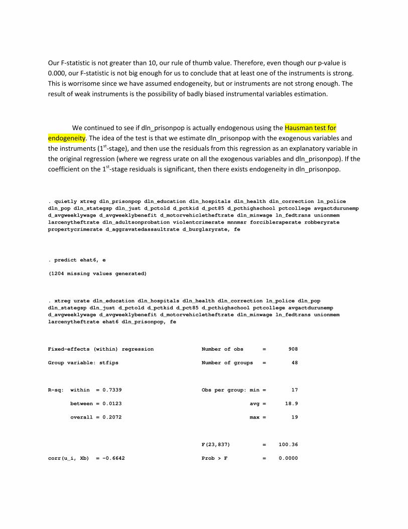
Our F-statistic is not greater than 10, our rule of thumb value. Therefore, even though our p-value is 0.000, our F-statistic is not big enough for us to conclude that at least one of the instruments is strong. This is worrisome since we have assumed endogeneity, but or instruments are not strong enough. The result of weak instruments is the possibility of badly biased instrumental variables estimation.

We continued to see if dln_prisonpop is actually endogenous using the Hausman test for endogeneity. The idea of the test is that we estimate dln_prisonpop with the exogenous variables and the instruments (1st-stage), and then use the residuals from this regression as an explanatory variable in the original regression (where we regress urate on all the exogenous variables and dln_prisonpop). If the coefficient on the 1st-stage residuals is significant, then there exists endogeneity in dln_prisonpop.

. quietly xtreg dln_prisonpop dln_education dln_hospitals dln_health dln_correction ln_police dln_pop dln_stategsp dln_just d_pctold d_pctkid d_pct85 d_pcthighschool pctcollege avgactdurunemp d_avgweeklywage d_avgweeklybenefit d_motorvehicletheftrate dln_minwage ln_fedtrans unionmem larcenytheftrate dln_adultsonprobation violentcrimerate mnnmsr forcibleraperate robberyrate propertycrimerate d_aggravatedassaultrate d_burglaryrate, fe

. predict ehat6, e

(1204 missing values generated)

. xtreg urate dln_education dln_hospitals dln_health dln_correction ln_police dln_pop dln_stategsp dln_just d_pctold d_pctkid d_pct85 d_pcthighschool pctcollege avgactdurunemp d_avgweeklywage d_avgweeklybenefit d_motorvehicletheftrate dln_minwage ln_fedtrans unionmem larcenytheftrate ehat6 dln_prisonpop, fe

Fixed-effects (within) regression Number of obs = 908

Group variable: stfips Number of groups = 48

R-sq: within = 0.7339 Obs per group: min = 17

between = 0.0123 avg = 18.9

overall = 0.2072 max = 19

F(23,837) = 100.36

corr(u_i, Xb) = -0.6642 Prob > F = 0.0000

-----------------------------------------------------------------------------------------

urate | Coef. Std. Err. t P>|t| [95% Conf. Interval]

------------------------+----------------------------------------------------------------

dln_education | -.5887862 .4966898 -1.19 0.236 -1.56369 .3861176

dln_hospitals | -.4535484 .2447103 -1.85 0.064 -.9338664 .0267695

dln_health | .1160472 .2448584 0.47 0.636 -.3645614 .5966559

dln_correction | -.2910745 .295184 -0.99 0.324 -.8704623 .2883133

ln_police | -.4491624 .1524956 -2.95 0.003 -.748481 -.1498438

dln_pop | -2.714675 2.198564 -1.23 0.217 -7.030021 1.60067

dln_stategsp | -5.458705 1.172403 -4.66 0.000 -7.7599 -3.157509

dln_just | -.0340231 .0507412 -0.67 0.503 -.133618 .0655718

d_pctold | 8.095799 10.92099 0.74 0.459 -13.33995 29.53154

d_pctkid | -4.776816 8.304302 -0.58 0.565 -21.07652 11.52289

d_pct85 | -33.86556 46.03796 -0.74 0.462 -124.229 56.49785

d_pcthighschool | .0042987 .0468051 0.09 0.927 -.0875705 .0961679

pctcollege | -.015103 .0213642 -0.71 0.480 -.0570368 .0268308

avgactdurunemp | .5184034 .0236629 21.91 0.000 .4719578 .5648491

d_avgweeklywage | -.0169876 .0042142 -4.03 0.000 -.0252593 -.0087159

d_avgweeklybenefit | -.0207814 .0043769 -4.75 0.000 -.0293724 -.0121903

d_motorvehicletheftrate | -.0019587 .0006931 -2.83 0.005 -.0033191 -.0005982

dln_minwage | .2054964 .2988495 0.69 0.492 -.381086 .7920788

ln_fedtrans | -1.00838 .1558634 -6.47 0.000 -1.314309 -.7024512

unionmem | .1714825 .0249651 6.87 0.000 .1224808 .2204841

larcenytheftrate | -.0003643 .0001069 -3.41 0.001 -.0005741 -.0001544

ehat6 | .7537365 1.969273 0.38 0.702 -3.111557 4.61903

dln_prisonpop | -2.579371 1.9212 -1.34 0.180 -6.350307 1.191566

_cons | 11.29029 1.574641 7.17 0.000 8.199585 14.381

------------------------+----------------------------------------------------------------

sigma_u | 2.0817598

sigma_e | .8325815

rho | .86210393 (fraction of variance due to u_i)

-----------------------------------------------------------------------------------------

F test that all u_i=0: F(47, 837) = 27.22 Prob > F = 0.0000

Based on our regression results, we find that the coefficient on the residuals (ehat6) is actually insignificant with a p-value of 0.702, thus it is possible that the variable dln_prisonpop is not endogenous in the first place. Therefore, we should be able to interpret the effect of the growth rate of prison population on the unemployment rate in the fixed effects model both statistically and economically without worrying too much about endogeneity bias. Note that sincewe found our instruments to be valid but weak, the Hausman test for endogeneity might still produce questionable results. Therefore, we don’t have enough information to prove or disprove endogeneity of the dln_prisonpop variable.

APPENDIX A.1

Dickey Fuller Tests for Nonstationarity (xtunitroot fisher [var], dfuller lags() [options])

UNEMPLOYMENT RATE

. xtunitroot fisher urate, dfuller lags(0) (48 missing values generated) Fisher-type unit-root test for urate Based on augmented Dickey-Fuller tests -------------------------------------- Ho: All panels contain unit roots Number of panels = 48 Ha: At least one panel is stationary Number of periods = 43 AR parameter: Panel-specific Asymptotics: T -> Infinity Panel means: Included Time trend: Not included Drift term: Not included ADF regressions: 0 lags ------------------------------------------------------------------------------ Statistic p-value ------------------------------------------------------------------------------ Inverse chi-squared(96) P 146.2396 0.0007 Inverse normal Z -5.0082 0.0000 Inverse logit t(244) L* -4.6531 0.0000 Modified inv. chi-squared Pm 3.6257 0.0001 ------------------------------------------------------------------------------ P statistic requires number of panels to be finite. Other statistics are suitable for finite or infinite number of panels. ------------------------------------------------------------------------------ Reject the null hypothesis that all the panels contain a unit root. => stationary

STATE GOVERNMENT EXPENDITURES

~Education

. xtunitroot fisher ln_education, dfuller lags(0) trend Fisher-type unit-root test for ln_education Based on augmented Dickey-Fuller tests ------------------------------------------- Ho: All panels contain unit roots Number of panels = 48 Ha: At least one panel is stationary Number of periods = 44 AR parameter: Panel-specific Asymptotics: T -> Infinity Panel means: Included Time trend: Included Drift term: Not included ADF regressions: 0 lags ------------------------------------------------------------------------------ Statistic p-value ------------------------------------------------------------------------------ Inverse chi-squared(96) P 109.6073 0.1619 Inverse normal Z 1.3079 0.9045 Inverse logit t(244) L* 0.9953 0.8397 Modified inv. chi-squared Pm 0.9820 0.1630 ------------------------------------------------------------------------------ P statistic requires number of panels to be finite. Other statistics are suitable for finite or infinite number of panels. ------------------------------------------------------------------------------ Fail to reject the null hypothesis that all the panels contain a unit root. => nonstationary

~Public Welfare . xtunitroot fisher ln_publicwelfare, dfuller lags(0) trend

Fisher-type unit-root test for ln_publicwelfare Based on augmented Dickey-Fuller tests ----------------------------------------------- Ho: All panels contain unit roots Number of panels = 48 Ha: At least one panel is stationary Number of periods = 44 AR parameter: Panel-specific Asymptotics: T -> Infinity Panel means: Included Time trend: Included Drift term: Not included ADF regressions: 0 lags ------------------------------------------------------------------------------ Statistic p-value ------------------------------------------------------------------------------ Inverse chi-squared(96) P 143.3923 0.0012 Inverse normal Z -0.6985 0.2424 Inverse logit t(244) L* -1.2383 0.1084 Modified inv. chi-squared Pm 3.4202 0.0003 ------------------------------------------------------------------------------ P statistic requires number of panels to be finite. Other statistics are suitable for finite or infinite number of panels. ------------------------------------------------------------------------------ Reject the null hypothesis that all the panels contain a unit root. => stationary

~Hospitals . xtunitroot fisher ln_hospitals, dfuller lags(0) trend (1 missing value generated) Fisher-type unit-root test for ln_hospitals Based on augmented Dickey-Fuller tests ------------------------------------------- Ho: All panels contain unit roots Number of panels = 48 Ha: At least one panel is stationary Avg. number of periods = 43.98 AR parameter: Panel-specific Asymptotics: T -> Infinity Panel means: Included Time trend: Included Drift term: Not included ADF regressions: 0 lags ------------------------------------------------------------------------------ Statistic p-value ------------------------------------------------------------------------------ Inverse chi-squared(96) P 91.2490 0.6180 Inverse normal Z 0.5814 0.7195 Inverse logit t(244) L* 0.4943 0.6892 Modified inv. chi-squared Pm -0.3429 0.6342 ------------------------------------------------------------------------------ P statistic requires number of panels to be finite. Other statistics are suitable for finite or infinite number of panels. ------------------------------------------------------------------------------ Fail to reject the null hypothesis that all the panels contain a unit root. => nonstationary

~Health . xtunitroot fisher ln_health, dfuller lags(0) trend Fisher-type unit-root test for ln_health Based on augmented Dickey-Fuller tests ---------------------------------------- Ho: All panels contain unit roots Number of panels = 48 Ha: At least one panel is stationary Number of periods = 44 AR parameter: Panel-specific Asymptotics: T -> Infinity Panel means: Included Time trend: Included

Drift term: Not included ADF regressions: 0 lags ------------------------------------------------------------------------------ Statistic p-value ------------------------------------------------------------------------------ Inverse chi-squared(96) P 42.3491 1.0000 Inverse normal Z 6.7919 1.0000 Inverse logit t(244) L* 6.8868 1.0000 Modified inv. chi-squared Pm -3.8719 0.9999 ------------------------------------------------------------------------------ P statistic requires number of panels to be finite. Other statistics are suitable for finite or infinite number of panels. ------------------------------------------------------------------------------ Fail to reject the null hypothesis that all the panels contain a unit root. => nonstationary

~Corrections . xtunitroot fisher ln_correction, dfuller lags(0) trend Fisher-type unit-root test for ln_correction Based on augmented Dickey-Fuller tests -------------------------------------------- Ho: All panels contain unit roots Number of panels = 48 Ha: At least one panel is stationary Number of periods = 44 AR parameter: Panel-specific Asymptotics: T -> Infinity Panel means: Included Time trend: Included Drift term: Not included ADF regressions: 0 lags ------------------------------------------------------------------------------ Statistic p-value ------------------------------------------------------------------------------ Inverse chi-squared(96) P 78.4685 0.9037 Inverse normal Z 9.2428 1.0000 Inverse logit t(234) L* 8.7687 1.0000 Modified inv. chi-squared Pm -1.2652 0.8971 ------------------------------------------------------------------------------ P statistic requires number of panels to be finite. Other statistics are suitable for finite or infinite number of panels. ------------------------------------------------------------------------------ Fail to reject the null hypothesis that all the panels contain a unit root. => nonstationary

~Police . xtunitroot fisher ln_police, dfuller lags(0) trend Fisher-type unit-root test for ln_police Based on augmented Dickey-Fuller tests ---------------------------------------- Ho: All panels contain unit roots Number of panels = 48 Ha: At least one panel is stationary Number of periods = 44 AR parameter: Panel-specific Asymptotics: T -> Infinity Panel means: Included Time trend: Included Drift term: Not included ADF regressions: 0 lags ------------------------------------------------------------------------------ Statistic p-value ------------------------------------------------------------------------------ Inverse chi-squared(96) P 214.6505 0.0000 Inverse normal Z -3.3690 0.0004 Inverse logit t(244) L* -5.1939 0.0000 Modified inv. chi-squared Pm 8.5629 0.0000 ------------------------------------------------------------------------------ P statistic requires number of panels to be finite.

Other statistics are suitable for finite or infinite number of panels. ------------------------------------------------------------------------------ Reject the null hypothesis that all the panels contain a unit root. => stationary

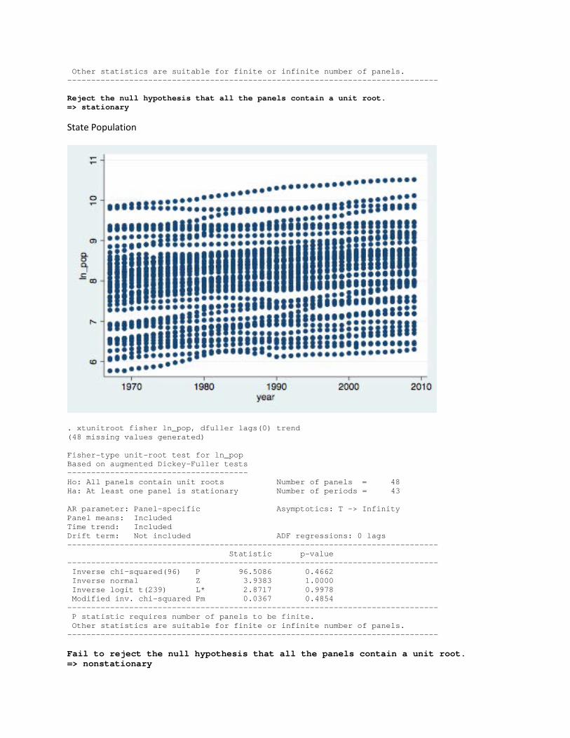
State Population

. xtunitroot fisher ln_pop, dfuller lags(0) trend (48 missing values generated) Fisher-type unit-root test for ln_pop Based on augmented Dickey-Fuller tests -------------------------------------- Ho: All panels contain unit roots Number of panels = 48 Ha: At least one panel is stationary Number of periods = 43 AR parameter: Panel-specific Asymptotics: T -> Infinity Panel means: Included Time trend: Included Drift term: Not included ADF regressions: 0 lags ------------------------------------------------------------------------------ Statistic p-value ------------------------------------------------------------------------------ Inverse chi-squared(96) P 96.5086 0.4662 Inverse normal Z 3.9383 1.0000 Inverse logit t(239) L* 2.8717 0.9978 Modified inv. chi-squared Pm 0.0367 0.4854 ------------------------------------------------------------------------------ P statistic requires number of panels to be finite. Other statistics are suitable for finite or infinite number of panels. ------------------------------------------------------------------------------ Fail to reject the null hypothesis that all the panels contain a unit root. => nonstationary

STATE FINANCES AND OUTPUT

~Gross State Product (GSP) . xtunitroot fisher ln_stategsp, dfuller lags(0) trend (48 missing values generated) Fisher-type unit-root test for ln_stategsp Based on augmented Dickey-Fuller tests ------------------------------------------ Ho: All panels contain unit roots Number of panels = 48 Ha: At least one panel is stationary Avg. number of periods = 43.00 AR parameter: Panel-specific Asymptotics: T -> Infinity Panel means: Included Time trend: Included Drift term: Not included ADF regressions: 0 lags ------------------------------------------------------------------------------ Statistic p-value ------------------------------------------------------------------------------ Inverse chi-squared(96) P 6.7767 1.0000 Inverse normal Z 12.7304 1.0000 Inverse logit t(214) L* 13.9424 1.0000 Modified inv. chi-squared Pm -6.4391 1.0000 ------------------------------------------------------------------------------ P statistic requires number of panels to be finite. Other statistics are suitable for finite or infinite number of panels. ------------------------------------------------------------------------------ Fail to reject the null hypothesis that all the panels contain a unit root. => nonstationary

~Debt . xtunitroot fisher ln_debt, dfuller lags(0) trend (144 missing values generated) Fisher-type unit-root test for ln_debt Based on augmented Dickey-Fuller tests -------------------------------------- Ho: All panels contain unit roots Number of panels = 48 Ha: At least one panel is stationary Number of periods = 41 AR parameter: Panel-specific Asymptotics: T -> Infinity Panel means: Included Time trend: Included Drift term: Not included ADF regressions: 0 lags ------------------------------------------------------------------------------ Statistic p-value ------------------------------------------------------------------------------ Inverse chi-squared(96) P 114.2241 0.0990 Inverse normal Z 4.0875 1.0000 Inverse logit t(244) L* 3.1070 0.9989 Modified inv. chi-squared Pm 1.3152 0.0942 ------------------------------------------------------------------------------ P statistic requires number of panels to be finite. Other statistics are suitable for finite or infinite number of panels. ------------------------------------------------------------------------------ Fail to reject the null hypothesis that all the panels contain a unit root. => nonstationary

~Federal Transfer of Funding . xtunitroot fisher ln_fedtrans, dfuller lags(0) trend (384 missing values generated) Fisher-type unit-root test for ln_fedtrans Based on augmented Dickey-Fuller tests ------------------------------------------ Ho: All panels contain unit roots Number of panels = 48 Ha: At least one panel is stationary Number of periods = 36 AR parameter: Panel-specific Asymptotics: T -> Infinity Panel means: Included Time trend: Included Drift term: Not included ADF regressions: 0 lags ------------------------------------------------------------------------------ Statistic p-value ------------------------------------------------------------------------------ Inverse chi-squared(96) P 201.8959 0.0000 Inverse normal Z -4.1439 0.0000 Inverse logit t(244) L* -5.5848 0.0000 Modified inv. chi-squared Pm 7.6424 0.0000 ------------------------------------------------------------------------------ P statistic requires number of panels to be finite. Other statistics are suitable for finite or infinite number of panels. ------------------------------------------------------------------------------ Reject the null hypothesis that all the panels contain a unit root. => stationary

~Department of Justice Spending in the State . xtunitroot fisher ln_just, dfuller lags(0) (530 missing values generated) Fisher-type unit-root test for ln_just Based on augmented Dickey-Fuller tests --------------------------------------

Ho: All panels contain unit roots Number of panels = 48 Ha: At least one panel is stationary Avg. number of periods = 32.96 AR parameter: Panel-specific Asymptotics: T -> Infinity Panel means: Included Time trend: Not included Drift term: Not included ADF regressions: 0 lags ------------------------------------------------------------------------------ Statistic p-value ------------------------------------------------------------------------------ Inverse chi-squared(96) P 34.5351 1.0000 Inverse normal Z 4.7089 1.0000 Inverse logit t(244) L* 4.2758 1.0000 Modified inv. chi-squared Pm -4.4359 1.0000 ------------------------------------------------------------------------------ P statistic requires number of panels to be finite. Other statistics are suitable for finite or infinite number of panels. ------------------------------------------------------------------------------ Fail to reject the null hypothesis that all the panels contain a unit root. => nonstationary

PRISON RELATED STATISTICS

~Adults on Probation in the State . xtunitroot fisher ln_adultsonprobation, dfuller lags(0) trend (495 missing values generated) Fisher-type unit-root test for ln_adultsonprobation Based on augmented Dickey-Fuller tests --------------------------------------------------- Ho: All panels contain unit roots Number of panels = 48 Ha: At least one panel is stationary Avg. number of periods = 33.69

AR parameter: Panel-specific Asymptotics: T -> Infinity Panel means: Included Time trend: Included Drift term: Not included ADF regressions: 0 lags ------------------------------------------------------------------------------ Statistic p-value ------------------------------------------------------------------------------ Inverse chi-squared(96) P 64.0805 0.9950 Inverse normal Z 7.4227 1.0000 Inverse logit t(194) L* 7.2999 1.0000 Modified inv. chi-squared Pm -2.3036 0.9894 ------------------------------------------------------------------------------ P statistic requires number of panels to be finite. Other statistics are suitable for finite or infinite number of panels. ------------------------------------------------------------------------------ Fail to reject the null hypothesis that all the panels contain a unit root. => nonstationary

~State Prison Population . xtunitroot fisher ln_prisonpop, dfuller lags(0) trend (480 missing values generated) Fisher-type unit-root test for ln_prisonpop Based on augmented Dickey-Fuller tests ------------------------------------------- Ho: All panels contain unit roots Number of panels = 48 Ha: At least one panel is stationary Avg. number of periods = 34.00 AR parameter: Panel-specific Asymptotics: T -> Infinity Panel means: Included Time trend: Included Drift term: Not included ADF regressions: 0 lags ------------------------------------------------------------------------------ Statistic p-value ------------------------------------------------------------------------------ Inverse chi-squared(96) P 22.0076 1.0000 Inverse normal Z 9.4937 1.0000 Inverse logit t(239) L* 10.0475 1.0000 Modified inv. chi-squared Pm -5.3399 1.0000 ------------------------------------------------------------------------------ P statistic requires number of panels to be finite. Other statistics are suitable for finite or infinite number of panels. ------------------------------------------------------------------------------ Fail to reject the null hypothesis that all the panels contain a unit root. => nonstationary

AGE DEMOGRAPHICS

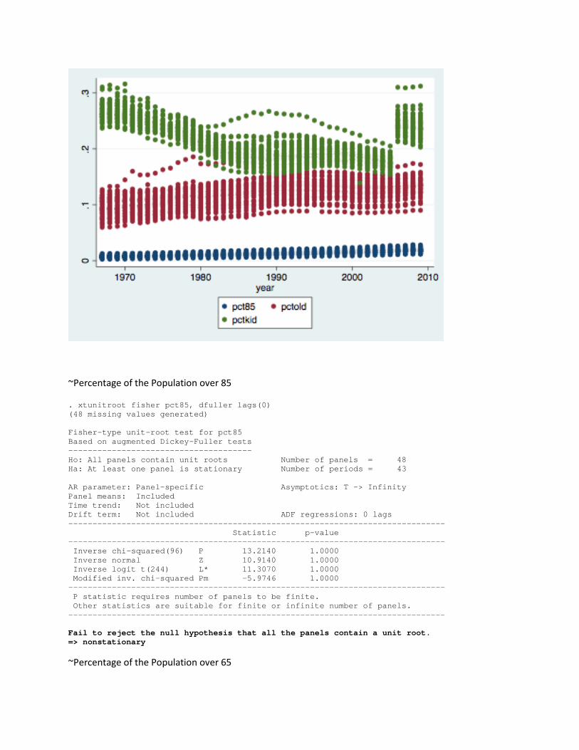
~Percentage of the Population over 85

. xtunitroot fisher pct85, dfuller lags(0) (48 missing values generated) Fisher-type unit-root test for pct85 Based on augmented Dickey-Fuller tests -------------------------------------- Ho: All panels contain unit roots Number of panels = 48 Ha: At least one panel is stationary Number of periods = 43 AR parameter: Panel-specific Asymptotics: T -> Infinity Panel means: Included Time trend: Not included Drift term: Not included ADF regressions: 0 lags ------------------------------------------------------------------------------ Statistic p-value ------------------------------------------------------------------------------ Inverse chi-squared(96) P 13.2140 1.0000 Inverse normal Z 10.9140 1.0000 Inverse logit t(244) L* 11.3070 1.0000 Modified inv. chi-squared Pm -5.9746 1.0000 ------------------------------------------------------------------------------ P statistic requires number of panels to be finite. Other statistics are suitable for finite or infinite number of panels. ------------------------------------------------------------------------------ Fail to reject the null hypothesis that all the panels contain a unit root. => nonstationary

~Percentage of the Population over 65

. xtunitroot fisher pctold, dfuller lags(0) trend (48 missing values generated) Fisher-type unit-root test for pctold Based on augmented Dickey-Fuller tests -------------------------------------- Ho: All panels contain unit roots Number of panels = 48 Ha: At least one panel is stationary Number of periods = 43 AR parameter: Panel-specific Asymptotics: T -> Infinity Panel means: Included Time trend: Included Drift term: Not included ADF regressions: 0 lags ------------------------------------------------------------------------------ Statistic p-value ------------------------------------------------------------------------------ Inverse chi-squared(96) P 77.3286 0.9188 Inverse normal Z 4.0906 1.0000 Inverse logit t(239) L* 3.8782 0.9999 Modified inv. chi-squared Pm -1.3475 0.9111 ------------------------------------------------------------------------------ P statistic requires number of panels to be finite. Other statistics are suitable for finite or infinite number of panels. ------------------------------------------------------------------------------ Fail to reject the null hypothesis that all the panels contain a unit root. => nonstationary

~Percentage of the Population between 5-17

. xtunitroot fisher pctkid, dfuller lags(0) trend (48 missing values generated) Fisher-type unit-root test for pctkid Based on augmented Dickey-Fuller tests -------------------------------------- Ho: All panels contain unit roots Number of panels = 48 Ha: At least one panel is stationary Number of periods = 43 AR parameter: Panel-specific Asymptotics: T -> Infinity Panel means: Included Time trend: Included Drift term: Not included ADF regressions: 0 lags ------------------------------------------------------------------------------ Statistic p-value ------------------------------------------------------------------------------ Inverse chi-squared(96) P 3.6677 1.0000 Inverse normal Z 13.2208 1.0000 Inverse logit t(244) L* 13.7289 1.0000 Modified inv. chi-squared Pm -6.6635 1.0000 ------------------------------------------------------------------------------ P statistic requires number of panels to be finite. Other statistics are suitable for finite or infinite number of panels. ------------------------------------------------------------------------------ Fail to reject the null hypothesis that all the panels contain a unit root. => nonstationary

EDUCATION DEMOGRAPHICS

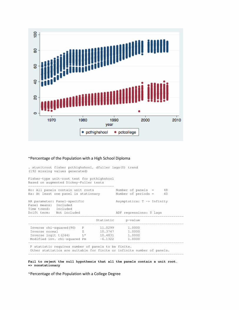
~Percentage of the Population with a High School Diploma

. xtunitroot fisher pcthighshool, dfuller lags(0) trend (192 missing values generated) Fisher-type unit-root test for pcthighshool Based on augmented Dickey-Fuller tests ------------------------------------------- Ho: All panels contain unit roots Number of panels = 48 Ha: At least one panel is stationary Number of periods = 40 AR parameter: Panel-specific Asymptotics: T -> Infinity Panel means: Included Time trend: Included Drift term: Not included ADF regressions: 0 lags ------------------------------------------------------------------------------ Statistic p-value ------------------------------------------------------------------------------ Inverse chi-squared(96) P 11.0299 1.0000 Inverse normal Z 10.3747 1.0000 Inverse logit t(244) L* 10.4831 1.0000 Modified inv. chi-squared Pm -6.1322 1.0000 ------------------------------------------------------------------------------ P statistic requires number of panels to be finite. Other statistics are suitable for finite or infinite number of panels. ------------------------------------------------------------------------------ Fail to reject the null hypothesis that all the panels contain a unit root. => nonstationary

~Percentage of the Population with a College Degree

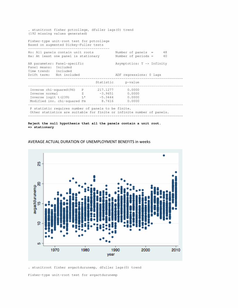
. xtunitroot fisher pctcollege, dfuller lags(0) trend (192 missing values generated) Fisher-type unit-root test for pctcollege Based on augmented Dickey-Fuller tests ----------------------------------------- Ho: All panels contain unit roots Number of panels = 48 Ha: At least one panel is stationary Number of periods = 40 AR parameter: Panel-specific Asymptotics: T -> Infinity Panel means: Included Time trend: Included Drift term: Not included ADF regressions: 0 lags ------------------------------------------------------------------------------ Statistic p-value ------------------------------------------------------------------------------ Inverse chi-squared(96) P 217.1277 0.0000 Inverse normal Z -3.9651 0.0000 Inverse logit t(239) L* -5.3444 0.0000 Modified inv. chi-squared Pm 8.7416 0.0000 ------------------------------------------------------------------------------ P statistic requires number of panels to be finite. Other statistics are suitable for finite or infinite number of panels. ------------------------------------------------------------------------------ Reject the null hypothesis that all the panels contain a unit root. => stationary

AVERAGE ACTUAL DURATION OF UNEMPLOYMENT BENEFITS in weeks

. xtunitroot fisher avgactdurunemp, dfuller lags(0) trend Fisher-type unit-root test for avgactdurunemp

Based on augmented Dickey-Fuller tests --------------------------------------------- Ho: All panels contain unit roots Number of panels = 48 Ha: At least one panel is stationary Number of periods = 44 AR parameter: Panel-specific Asymptotics: T -> Infinity Panel means: Included Time trend: Included Drift term: Not included ADF regressions: 0 lags ------------------------------------------------------------------------------ Statistic p-value ------------------------------------------------------------------------------ Inverse chi-squared(96) P 306.3697 0.0000 Inverse normal Z -10.4649 0.0000 Inverse logit t(244) L* -11.5001 0.0000 Modified inv. chi-squared Pm 15.1821 0.0000 ------------------------------------------------------------------------------ P statistic requires number of panels to be finite. Other statistics are suitable for finite or infinite number of panels. ------------------------------------------------------------------------------ Reject the null hypothesis that all the panels contain a unit root. => stationary

AVERAGE WEEKLY WAGE

. xtunitroot fisher avgweeklywage, dfuller lags(0) trend Fisher-type unit-root test for avgweeklywage Based on augmented Dickey-Fuller tests -------------------------------------------- Ho: All panels contain unit roots Number of panels = 48 Ha: At least one panel is stationary Number of periods = 44

AR parameter: Panel-specific Asymptotics: T -> Infinity Panel means: Included Time trend: Included Drift term: Not included ADF regressions: 0 lags ------------------------------------------------------------------------------ Statistic p-value ------------------------------------------------------------------------------ Inverse chi-squared(96) P 61.0690 0.9979 Inverse normal Z 2.8931 0.9981 Inverse logit t(239) L* 3.0378 0.9987 Modified inv. chi-squared Pm -2.5209 0.9941 ------------------------------------------------------------------------------ P statistic requires number of panels to be finite. Other statistics are suitable for finite or infinite number of panels. ------------------------------------------------------------------------------ Fail to reject the null hypothesis that all the panels contain a unit root. => nonstationary

AVERAGE WEEKLY UNEMPLOYMENT BENEFITS

. xtunitroot fisher avgweeklybenefit, dfuller lags(0) trend Fisher-type unit-root test for avgweeklybenefit Based on augmented Dickey-Fuller tests ----------------------------------------------- Ho: All panels contain unit roots Number of panels = 48 Ha: At least one panel is stationary Number of periods = 44 AR parameter: Panel-specific Asymptotics: T -> Infinity Panel means: Included Time trend: Included Drift term: Not included ADF regressions: 0 lags ------------------------------------------------------------------------------

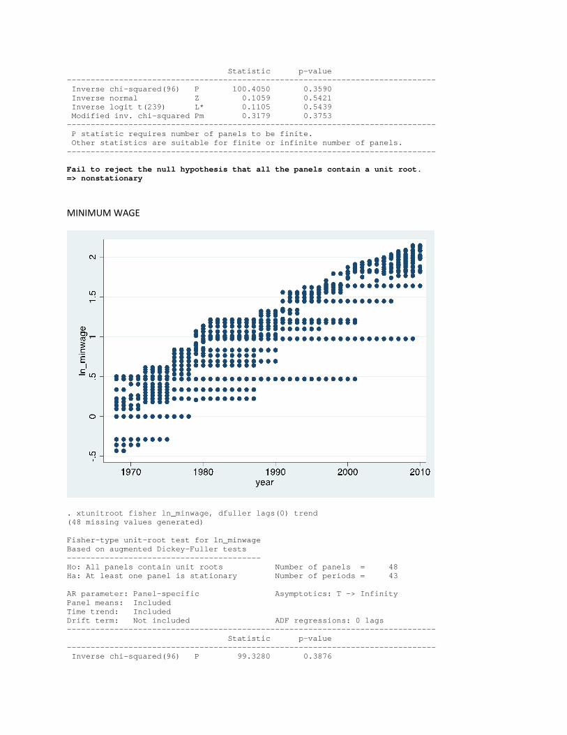
Statistic p-value ------------------------------------------------------------------------------ Inverse chi-squared(96) P 100.4050 0.3590 Inverse normal Z 0.1059 0.5421 Inverse logit t(239) L* 0.1105 0.5439 Modified inv. chi-squared Pm 0.3179 0.3753 ------------------------------------------------------------------------------ P statistic requires number of panels to be finite. Other statistics are suitable for finite or infinite number of panels. ------------------------------------------------------------------------------ Fail to reject the null hypothesis that all the panels contain a unit root. => nonstationary

MINIMUM WAGE

. xtunitroot fisher ln_minwage, dfuller lags(0) trend (48 missing values generated) Fisher-type unit-root test for ln_minwage Based on augmented Dickey-Fuller tests ----------------------------------------- Ho: All panels contain unit roots Number of panels = 48 Ha: At least one panel is stationary Number of periods = 43 AR parameter: Panel-specific Asymptotics: T -> Infinity Panel means: Included Time trend: Included Drift term: Not included ADF regressions: 0 lags ------------------------------------------------------------------------------ Statistic p-value ------------------------------------------------------------------------------ Inverse chi-squared(96) P 99.3280 0.3876

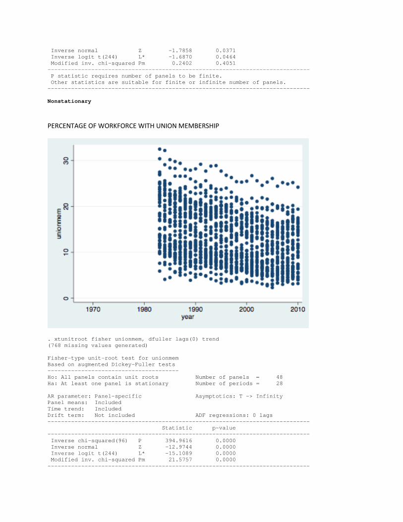
Inverse normal Z -1.7858 0.0371 Inverse logit t(244) L* -1.6870 0.0464 Modified inv. chi-squared Pm 0.2402 0.4051 ------------------------------------------------------------------------------ P statistic requires number of panels to be finite. Other statistics are suitable for finite or infinite number of panels. ------------------------------------------------------------------------------ Nonstationary

PERCENTAGE OF WORKFORCE WITH UNION MEMBERSHIP

. xtunitroot fisher unionmem, dfuller lags(0) trend (768 missing values generated) Fisher-type unit-root test for unionmem Based on augmented Dickey-Fuller tests --------------------------------------- Ho: All panels contain unit roots Number of panels = 48 Ha: At least one panel is stationary Number of periods = 28 AR parameter: Panel-specific Asymptotics: T -> Infinity Panel means: Included Time trend: Included Drift term: Not included ADF regressions: 0 lags ------------------------------------------------------------------------------ Statistic p-value ------------------------------------------------------------------------------ Inverse chi-squared(96) P 394.9616 0.0000 Inverse normal Z -12.9744 0.0000 Inverse logit t(244) L* -15.1089 0.0000 Modified inv. chi-squared Pm 21.5757 0.0000 ------------------------------------------------------------------------------

P statistic requires number of panels to be finite. Other statistics are suitable for finite or infinite number of panels. ------------------------------------------------------------------------------ Reject the null hypothesis that all the panels contain a unit root.

=>Stationary

CONSUMER PRICE INDEX (CPI)

. xtunitroot fisher cpi, dfuller lags(0) trend (528 missing values generated) Fisher-type unit-root test for cpi Based on augmented Dickey-Fuller tests -------------------------------------- Ho: All panels contain unit roots Number of panels = 48 Ha: At least one panel is stationary Number of periods = 33 AR parameter: Panel-specific Asymptotics: T -> Infinity Panel means: Included Time trend: Included Drift term: Not included ADF regressions: 0 lags ------------------------------------------------------------------------------ Statistic p-value ------------------------------------------------------------------------------ Inverse chi-squared(96) P 2265.0036 0.0000 Inverse normal Z -44.6730 0.0000 Inverse logit t(244) L* -90.3076 0.0000 Modified inv. chi-squared Pm 156.5343 0.0000 ------------------------------------------------------------------------------ P statistic requires number of panels to be finite. Other statistics are suitable for finite or infinite number of panels. ------------------------------------------------------------------------------ Reject the null hypothesis that all the panels contain a unit root. => stationary

CRIME RATE STATISTICS

~Burglary Rate

. xtunitroot fisher burglaryrate, dfuller lags(0) Fisher-type unit-root test for burglaryrate Based on augmented Dickey-Fuller tests ------------------------------------------- Ho: All panels contain unit roots Number of panels = 48 Ha: At least one panel is stationary Number of periods = 44 AR parameter: Panel-specific Asymptotics: T -> Infinity Panel means: Included Time trend: Not included Drift term: Not included ADF regressions: 0 lags ------------------------------------------------------------------------------ Statistic p-value ------------------------------------------------------------------------------ Inverse chi-squared(96) P 75.2696 0.9419 Inverse normal Z 2.1857 0.9856 Inverse logit t(244) L* 2.0315 0.9784 Modified inv. chi-squared Pm -1.4961 0.9327 ------------------------------------------------------------------------------ P statistic requires number of panels to be finite. Other statistics are suitable for finite or infinite number of panels. ------------------------------------------------------------------------------ Nonstationary

~Larceny Theft Rate

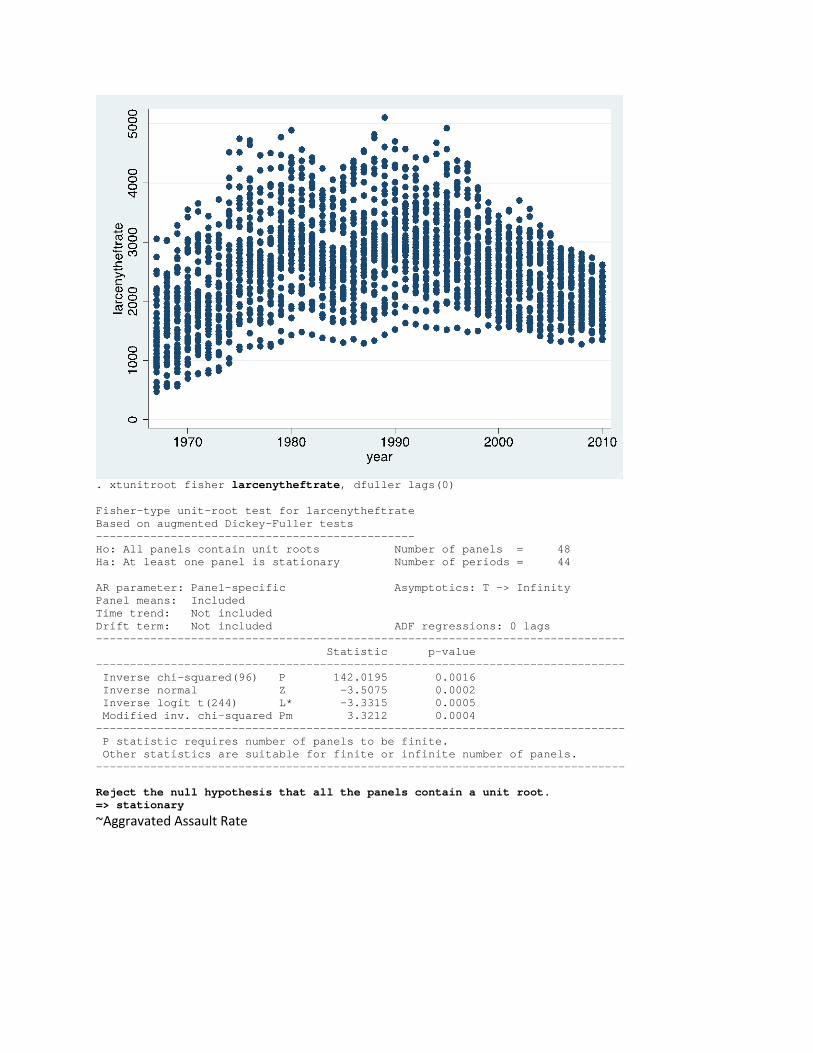
. xtunitroot fisher larcenytheftrate, dfuller lags(0) Fisher-type unit-root test for larcenytheftrate Based on augmented Dickey-Fuller tests ----------------------------------------------- Ho: All panels contain unit roots Number of panels = 48 Ha: At least one panel is stationary Number of periods = 44 AR parameter: Panel-specific Asymptotics: T -> Infinity Panel means: Included Time trend: Not included Drift term: Not included ADF regressions: 0 lags ------------------------------------------------------------------------------ Statistic p-value ------------------------------------------------------------------------------ Inverse chi-squared(96) P 142.0195 0.0016 Inverse normal Z -3.5075 0.0002 Inverse logit t(244) L* -3.3315 0.0005 Modified inv. chi-squared Pm 3.3212 0.0004 ------------------------------------------------------------------------------ P statistic requires number of panels to be finite. Other statistics are suitable for finite or infinite number of panels. ------------------------------------------------------------------------------ Reject the null hypothesis that all the panels contain a unit root. => stationary

~Aggravated Assault Rate

. xtunitroot fisher aggravatedassaultrate, dfuller lags(0) Fisher-type unit-root test for aggravatedassaultrate Based on augmented Dickey-Fuller tests ---------------------------------------------------- Ho: All panels contain unit roots Number of panels = 48 Ha: At least one panel is stationary Number of periods = 44 AR parameter: Panel-specific Asymptotics: T -> Infinity Panel means: Included Time trend: Not included Drift term: Not included ADF regressions: 0 lags ------------------------------------------------------------------------------ Statistic p-value ------------------------------------------------------------------------------ Inverse chi-squared(96) P 116.2495 0.0782 Inverse normal Z -2.6642 0.0039 Inverse logit t(244) L* -2.4391 0.0077 Modified inv. chi-squared Pm 1.4614 0.0720 ------------------------------------------------------------------------------ P statistic requires number of panels to be finite. Other statistics are suitable for finite or infinite number of panels. ------------------------------------------------------------------------------ Fail to reject the null hypothesis that all the panels contain a unit root. => nonstationary

~Property Crime Rate

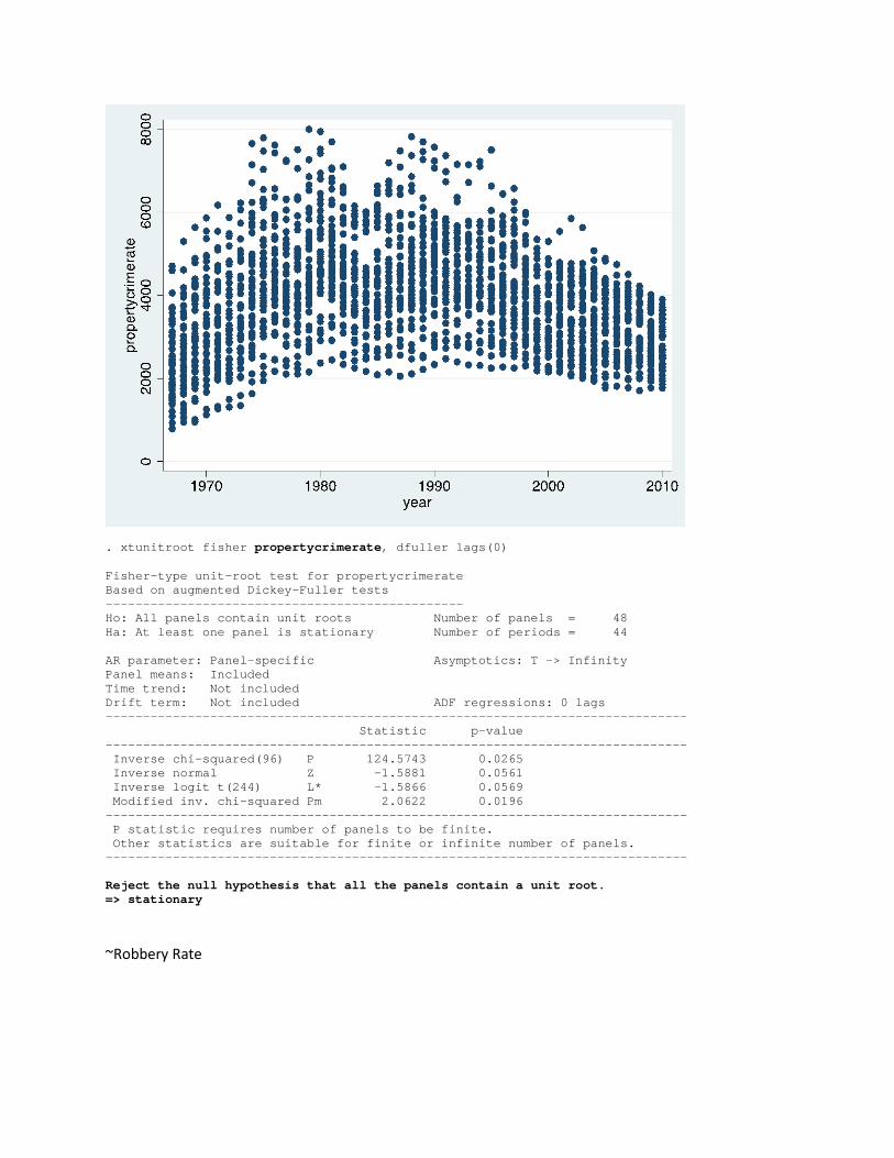
. xtunitroot fisher propertycrimerate, dfuller lags(0) Fisher-type unit-root test for propertycrimerate Based on augmented Dickey-Fuller tests ------------------------------------------------ Ho: All panels contain unit roots Number of panels = 48 Ha: At least one panel is stationary Number of periods = 44 AR parameter: Panel-specific Asymptotics: T -> Infinity Panel means: Included Time trend: Not included Drift term: Not included ADF regressions: 0 lags ------------------------------------------------------------------------------ Statistic p-value ------------------------------------------------------------------------------ Inverse chi-squared(96) P 124.5743 0.0265 Inverse normal Z -1.5881 0.0561 Inverse logit t(244) L* -1.5866 0.0569 Modified inv. chi-squared Pm 2.0622 0.0196 ------------------------------------------------------------------------------ P statistic requires number of panels to be finite. Other statistics are suitable for finite or infinite number of panels. ------------------------------------------------------------------------------ Reject the null hypothesis that all the panels contain a unit root. => stationary

~Robbery Rate

. xtunitroot fisher robberyrate, dfuller lags(0) Fisher-type unit-root test for robberyrate Based on augmented Dickey-Fuller tests ------------------------------------------ Ho: All panels contain unit roots Number of panels = 48 Ha: At least one panel is stationary Number of periods = 44 AR parameter: Panel-specific Asymptotics: T -> Infinity Panel means: Included Time trend: Not included Drift term: Not included ADF regressions: 0 lags ------------------------------------------------------------------------------ Statistic p-value ------------------------------------------------------------------------------ Inverse chi-squared(96) P 210.7856 0.0000 Inverse normal Z -6.6043 0.0000 Inverse logit t(244) L* -6.8868 0.0000 Modified inv. chi-squared Pm 8.2839 0.0000 ------------------------------------------------------------------------------ P statistic requires number of panels to be finite. Other statistics are suitable for finite or infinite number of panels. ------------------------------------------------------------------------------ Reject the null hypothesis that all the panels contain a unit root. => stationary

~Forcible Rape Rate

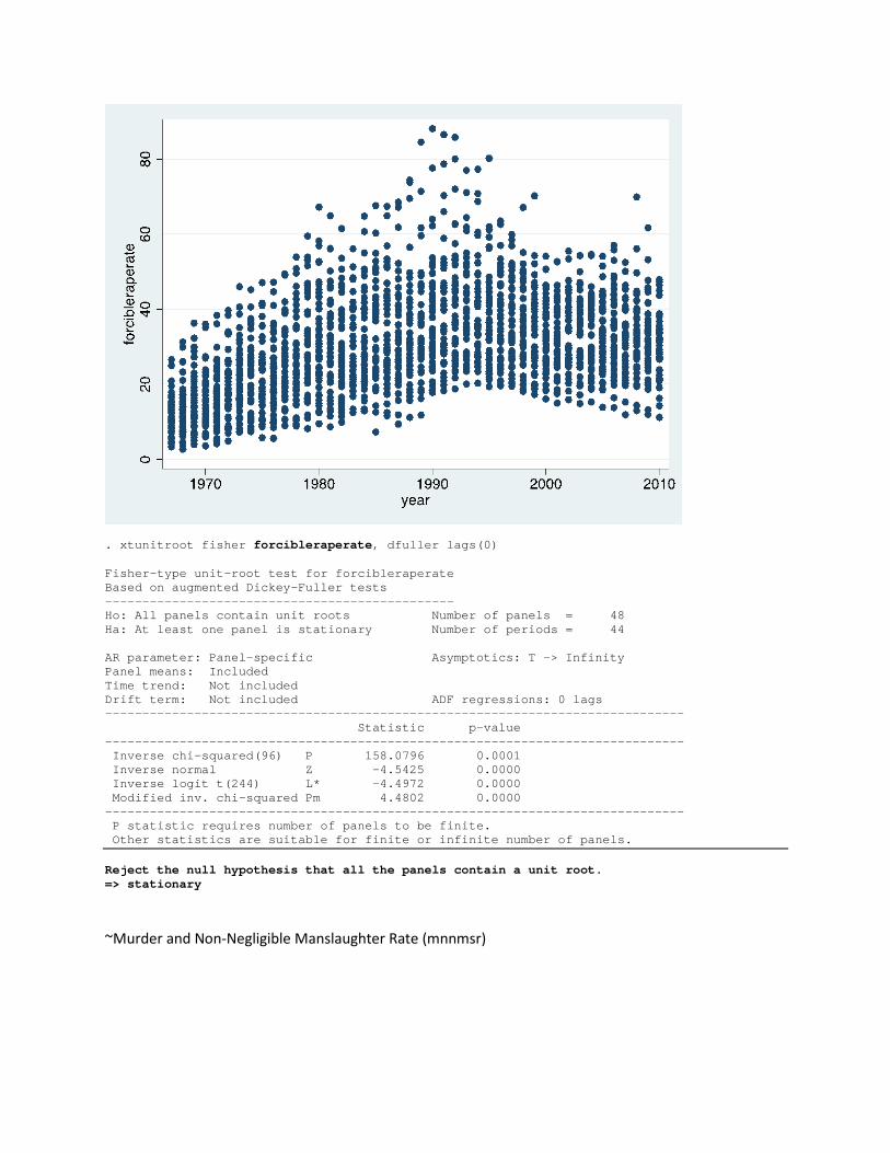
. xtunitroot fisher forcibleraperate, dfuller lags(0) Fisher-type unit-root test for forcibleraperate Based on augmented Dickey-Fuller tests ----------------------------------------------- Ho: All panels contain unit roots Number of panels = 48 Ha: At least one panel is stationary Number of periods = 44 AR parameter: Panel-specific Asymptotics: T -> Infinity Panel means: Included Time trend: Not included Drift term: Not included ADF regressions: 0 lags ------------------------------------------------------------------------------ Statistic p-value ------------------------------------------------------------------------------ Inverse chi-squared(96) P 158.0796 0.0001 Inverse normal Z -4.5425 0.0000 Inverse logit t(244) L* -4.4972 0.0000 Modified inv. chi-squared Pm 4.4802 0.0000 ------------------------------------------------------------------------------ P statistic requires number of panels to be finite. Other statistics are suitable for finite or infinite number of panels. Reject the null hypothesis that all the panels contain a unit root. => stationary

~Murder and Non-Negligible Manslaughter Rate (mnnmsr)

. xtunitroot fisher mnnmsr, dfuller lags(0) Fisher-type unit-root test for mnnmsr Based on augmented Dickey-Fuller tests -------------------------------------- Ho: All panels contain unit roots Number of panels = 48 Ha: At least one panel is stationary Number of periods = 44 AR parameter: Panel-specific Asymptotics: T -> Infinity Panel means: Included Time trend: Not included Drift term: Not included ADF regressions: 0 lags ------------------------------------------------------------------------------ Statistic p-value ------------------------------------------------------------------------------ Inverse chi-squared(96) P 360.0734 0.0000 Inverse normal Z -8.6354 0.0000 Inverse logit t(244) L* -12.2409 0.0000 Modified inv. chi-squared Pm 19.0579 0.0000 ------------------------------------------------------------------------------ P statistic requires number of panels to be finite. Other statistics are suitable for finite or infinite number of panels. ------------------------------------------------------------------------------ Reject the null hypothesis that all the panels contain a unit root. => stationary

~Violent Crime Rate

. xtunitroot fisher violentcrimerate, dfuller lags(0) Fisher-type unit-root test for violentcrimerate Based on augmented Dickey-Fuller tests ----------------------------------------------- Ho: All panels contain unit roots Number of panels = 48 Ha: At least one panel is stationary Number of periods = 44 AR parameter: Panel-specific Asymptotics: T -> Infinity Panel means: Included Time trend: Not included Drift term: Not included ADF regressions: 0 lags ------------------------------------------------------------------------------ Statistic p-value ------------------------------------------------------------------------------ Inverse chi-squared(96) P 150.4355 0.0003 Inverse normal Z -4.4483 0.0000 Inverse logit t(244) L* -4.2178 0.0000 Modified inv. chi-squared Pm 3.9285 0.0000 ------------------------------------------------------------------------------ P statistic requires number of panels to be finite. Other statistics are suitable for finite or infinite number of panels. ------------------------------------------------------------------------------ Reject the null hypothesis that all the panels contain a unit root. => stationary

Conclusion:

Despite weak results from the fixed effect 2SLS, this paper provides evidence that increasing growth rates of prison population likely has a negative relationship with unemployment, such that an increase in prison growth rate results in a decrease in the unemployment rate. This is

suggestive of what kind of response new policies directed at increased imprisonment also have a strong effect on unemployment.

However, we were not able to prove conclusively that an endogenous relationship exists between unemployment and prison population, which would have suggested that policies targeted at increasing imprisonment rates are enacted due to high unemployment.

Using VAR models we find evidence that unemployment and prison populations granger cause one another and are endogenous. However, due to weak instrumental variables we were unable accurately test endogeneity in our fixed effects model.

Validity Assessment:

As in most panel data sets omitted variable bias is a concern with the dataset used in this project. The most pertinent omitted variables in our project were those that dealt with both general and prison demographics. Problematically, data on demographics of the US prison population is not readily available. This is concerning due to the generally understood ethnic imbalance in prisons. Ultimately, we were unable to control for many population demographics which would have been useful in explaining both unemployment and prison rates.

Similarly, we lacked sufficiently strong instrumental variables to conduct a valid IV 2SLS regression. We lacked variables that we sufficiently correlated with prison population growth and without correlation to the unemployment rate. One variable that would have likely been useful would be prison demographics or crime specific policy implementation.

Another concern is that parts of our data set were derived from self-reported surveys which might incentivize over or under reporting. Prior to 2004 the UCR were used to rank law enforcement agencies, which may have resulted in over and under reporting of certain crimes.

Likewise, the US prison system is rife with selection bias. For one the vast majority of prisoners are male and not white. Further, certain crimes, such as those involving sexual assault, have social implications that might prevent the victim from coming forward. This may result in false trends resulting not from increased crime rates but increased reporting rates.

Further, we make a number of potentially problematic assumptions in this paper. One critical assumption that this paper makes about those imprisoned in US correctional facilities is that they share the same propensity to pursue employment as the general US population. This is particularly problematic if crime is dependent on particular characteristics. For instance if crime is only committed by meth addicts, and presumably meth addicts have lower rates of participation in the labor force for various reasons, it would not be valid to equate the employment profile of a criminal with a non-criminal due to self selection bias.

Another assumption that may be a problem is that crime is not committed out of necessity. Which is to say that high unemployment does not cause crime through channels of necessity. This is perhaps less of a concern than the prior assumption due to the well-documented geographic

invariance of crime.1 Concentrations of crime tend to be in low income transitionary neighborhoods with large population turnovers. During times of economic hardship crime is not exported to higher income targets but remains geographically stagnant.

1 The Geography of Crime Joseph Cohen Annals of the American Academy of Political and Social Science Vol. 217, Crime in the United States (Sep., 1941), pp. 29-37 Published by: Sage Publications, Inc. in association with the American Academy of Political and Social Science Stable URL: http://www.jstor.org/stable/1023412