TERRESTRIAL PLANET FORMATION AT HOME ANDABROAD

Sean N. RaymondLaboratoire d’Astrophysique de Bordeaux, CNRS and Universite de Bordeaux, 33270 Floirac, France

Eiichiro KokuboDivision of Theoretical Astronomy, National AstronomicalObservatory of Japan, Osawa, Mitaka, Tokyo, 181-8588, Japan

Alessandro MorbidelliLaboratoire Lagrange, Observatoire de la Cote d’Azur, Nice, France

Ryuji MorishimaUniversity of California, Los Angeles, Institute of Geophysics and Planetary Physics, Los Angeles, CA 90095, USA

Kevin J. WalshSouthwest Research Institute, Boulder, Colorado 80302, USA

We review the state of the field of terrestrial planet formation with the goal of understandingthe formation of the inner Solar System and low-mass exoplanets. We review the dynamics andtimescales of accretion from planetesimals to planetary embryos and from embryos to terrestrialplanets. We discuss radial mixing and water delivery, planetary spins and the importance ofparameters regarding the disk and embryo properties. Next,we connect accretion models toexoplanets. We first explain why the observed hot Super Earths probably formed by in situaccretion or inward migration. We show how terrestrial planet formation is altered in systemswith gas giants by the mechanisms of giant planet migration and dynamical instabilities.Standard models of terrestrial accretion fail to reproducethe inner Solar System. The “GrandTack” model solves this problem using ideas first developed to explain the giant exoplanets.Finally, we discuss whether most terrestrial planet systems form in the same way as ours, andhighlight the key ingredients missing in the current generation of simulations.

1. INTRODUCTION

The term “terrestrial planet” evokes landscapes of arocky planet like Earth or Mars but given recent discov-eries it has become somewhat ambiguous. Does a5 M⊕

Super Earth count as a terrestrial planet? What about theMars-sized moon of a giant planet? These objects are ter-restrial planet-sized but their compositions and correspond-ing landscapes probably differ significantly from our ter-restrial planets’. In addition, while Earth is thought to haveformed via successive collisions of planetesimals and plan-etary embryos, the other objects may have formed via dif-ferent mechanisms. For instance, under some conditions a10 M⊕ or larger body can form by accreting only planetes-imals, or even only cm-sized pebbles. In the context of theclassical stages of accretion this might be considered a “gi-ant embryo” rather than a planet (see§7.1).

What criteria should be used to classify a planet asterrestrial? A bulk density higher than a fewg cm−3

probably indicates a rock-dominated planet, but densitiesof low-mass exoplanets are extremely challenging to pindown (seeMarcy et al.2013). A planet with a bulk den-

sity of 0.5 − 2g cm−3 could either be rocky with a smallH-rich envelope or an ocean planet (Fortney et al.2007;Valencia et al.2007;Adams et al.2008). Bulk densitieslarger than3g cm−3 have been measured for planets as mas-sive as10 − 20 M⊕, although higher-density planets aregenerally smaller (Weiss et al.2013). Planets with radiiR . 1.5 − 2 R⊕ or massesM . 5 − 10 M⊕ are likely topreferentially have densities of3g cm−3 or larger and thusbe rocky (Weiss and Marcy2013;Lopez and Fortney2013).

In this review we address the formation of planets inorbit around stars that are between roughly a lunar mass(∼ 0.01 M⊕) and ten Earth masses. Although the com-positions of planets in this mass range certainly vary sub-stantially, these planets are capable of having solid sur-faces, whether they are covered by thick atmospheres ornot. These planets are also below the expected thresholdfor giant planet cores (e.g.Lissauer and Stevenson2007).We refer to these as terrestrial planets. We start our discus-sion of terrestrial planet formation when planetesimals havealready formed; for a discussion of planetesimal formationplease see the chapter by Johansen et al.

1

Our understanding of terrestrial planet formation hasundergone a dramatic improvement in recent years. Thiswas driven mainly by two factors: increased computationalpower and observations of extra-solar planets. Computingpower is the currency of numerical simulations, which con-tinually increase in resolution and have become more andmore complex and realistic. At the same time, dramatic ad-vances in exoplanetary science have encouraged many tal-ented young scientists to join the ranks of the planet for-mation community. This manpower and computing powerprovided a timely kick in the proverbial butt.

Despite the encouraging prognosis, planet formationmodels lag behind observations. Half of all Sun-like starsare orbited by close-in “super Earths”, yet we do not knowhow they form. There exist ideas as to why Mercury is somuch smaller than Earth and Venus but they remain spec-ulative and narrow. Only recently was a cohesive theorypresented to explain why Mars is smaller than Earth, andmore work is needed to confirm or refute it.

We first present the observational constraints in the So-lar System and extra-solar planetary systems in§2. Next,we review the dynamics of accretion of planetary embryosfrom planetesimals in§3, and of terrestrial planets from em-bryos in§4, including a discussion of the importance of arange of parameters. In§5 we apply accretion models toextra-solar planets and in§6 to the Solar System. We dis-cuss different modes of accretion and current limitations in§7 and summarize in§8.

2. OBSERVATIONAL CONSTRAINTS

Given the explosion of new discoveries in extra-solarplanets and our detailed knowledge of the Solar System,there are ample observations with which to constrain accre-tion models. Given the relatively low resolution of numer-ical simulations, accretion models generally attempt to re-produce large-scale constraints such as planetary mass-andorbital distributions rather than smaller-scale ones liketheexact characteristics of each planet. We now summarize thekey constraints for the Solar System and exoplanets.

2.1 The Solar System

The masses and orbits of the terrestrial planets.Thereexist metrics to quantify different aspects of a planetary sys-tem and to compare it with the Solar System. The angularmomentum deficitAMD (Laskar1997) measures the dif-ference in orbital angular momentum between the planets’orbits and the same planets on circular, coplanar orbits. TheAMD is generally used in its normalized form:

AMD =

∑

j mj√

aj

(

1 − cos(ij)√

1 − e2j

)

∑

j mj√

aj, (1)

whereaj , ej , ij, andmj are planetj’s semimajor axis, ec-centricity, inclination and mass. TheAMD of the SolarSystem’s terrestrial planets is 0.0018.

The radial mass concentrationRMC (defined asSc byChambers2001) measures the degree to which a system’smass is concentrated in a small region:

RMC = max

( ∑

mj∑

mj [log10(a/aj)]2

)

. (2)

Here, the function in brackets is calculated fora across theplanetary system, and theRMC is the maximum of thatfunction. For a single-planet system theRMC is infinite.The RMC is higher for systems in which the total massis packed in smaller and smaller radial zones. TheRMCis thus smaller for a system with equal-mass planets than asystem in which a subset of planets dominate the mass. TheRMC of the Solar System’s terrestrial planets is 89.9.

The geochemically-determined accretion histories ofEarth and Mars. Radiogenic elements with half-lives ofa few to 100 Myr can offer concrete constraints on the ac-cretion of the terrestrial planets. Of particular interestisthe182Hf-182W system, which has a half life of 9 Myr. Hfis lithophile (“rock-loving”) and W is siderophile (“iron-loving”). The amount of W in a planet’s mantle relative toHf depends on the timing of core formation (Nimmo andAgnor 2006). Early core formation (also called “core clo-sure”) would strand still-active Hf and later its product W inthe mantle, while late core formation would cause all W tobe sequestered in the core and leave behind a W-poor man-tle. Studies of the Hf-W system have concluded that thelast core formation event on Earth happened roughly 30-100Myr after the start of planet formation (Kleine et al.2002;Yin et al.2002;Kleine et al.2009;Konig et al.2011). Simi-lar studies on martian meteorites show that Mars’ accretionfinished far earlier, within 5 Myr (Nimmo and Kleine2007;Dauphas and Pourmand2011).

The highly-siderophile element (HSE) contents of theterrestrial planets’ mantles also provide constraints on thetotal amount of mass accreted by a planet after core clo-sure (Drake and Righter2002). This phase of accretion iscalled thelate veneer(Kimura et al.1974). Several un-solved problems exist regarding the late veneer, notablythe very high Earth/Moon HSE abundance ratio (Day et al.2007;Walker2009), which has been proposed to be the re-sult of either a top-heavy (Bottke et al.2010;Raymond et al.2013) or bottom-heavy (Schlichting et al.2012) distributionof planetesimal masses.

The large-scale structure of the asteroid belt.Repro-ducing the asteroid belt is not the main objective of forma-tion models. But any successful accretion model must beconsistent with the asteroid belt’s observed structure, andthat structure can offer valuable information about planetformation. Populations of small bodies can be thought of asthe “blood spatter on the wall” that helps detectives solvethe “crime”, figuratively speaking of course.

The asteroid belt’s total mass is just5×10−4 M⊕, aboutfour percent of a lunar mass. This is 3-4 orders of magni-tude smaller than the mass contained within the belt for anydisk surface density profile with a smooth radial slope. Inaddition, the inner belt is dominated by more volatile-poor

2

bodies such as E-types and S-types whereas the outer beltcontains more volatile-rich bodies such as C-types and D-types (Gradie and Tedesco1982;DeMeo and Carry2013).There are no large gaps in the distribution of asteroids– apart from the Kirkwood gaps associated with strongresonances with Jupiter – and this indicates that no large(& 0.05 M⊕) embryos were stranded in the belt after accre-tion, even if the embryos could have been removed duringthe late heavy bombardment (Raymond et al.2009).

The existence and abundance of volatile species – es-pecially water – on Earth. Although it contains just 0.05-0.1% water by mass (Lecuyer et al.1998; Marty 2012),Earth is the wettest terrestrial planet. It is as wet as ordi-nary chondrite meteorites, thought to represent the S-typeasteroids that dominate the inner main belt, and wetter thanenstatite chondrites that represent E-types interior to themain belt (see, for example, figure 5 fromMorbidelli et al.2012). We think that this means that the rocky buildingblocks in the inner Solar System were dry. In addition, heat-ing mechanisms such as collisional heating and radiogenicheating from26Al may have dehydrated fast-forming plan-etesimals (e.g.Grimm and McSween1993). The source ofEarth’s water therefore requires an explanation.

The isotopic composition of Earth’s water constrains itsorigins. The D/H ratio of water on Earth is a good match tocarbonaceous chondrite meteorites thought to originate inthe outer asteroid belt (Marty and Yokochi2006). The D/Hof most observed comets is2× higher – although one cometwas recently measured to have the same D/H as Earth (Har-togh et al.2011) – and that of the Sun (and presumablythe gaseous component of the protoplanetary disk) is6×smaller (Geiss and Gloeckler1998). It is interesting to notethat, while the D/H of Earth’s water can be matched with aweighted mixture of material with Solar and cometary D/H,that same combination does not match the15N/14N isotopicratio (Marty and Yokochi2006). Carbonaceous chondrites,on the other hand, match both measured ratios.

The bulk compositions of the planets are another con-straint. For example, the core/mantle (iron/silicate) massratideo of the terrestrial planets ranges from 0.4 (Mars) to2.1 (Mercury). The bulk compositions of the terrestrialplanets depend on several factors in addition to orbital dy-namics and accretion: the initial compositional gradientsofembryos and planetesimals, evolving condensation fronts,and the compositional evolution of bodies due to collisions

Key inner Solar System ConstraintsAngular momentum deficitAMD 0.0018Radial Mass ConcentrationRMC 89.9Mars’ accretion timescale1 3-5 MyrEarth’s accretion timescale2

∼ 50 MyrEarth’s late veneer3 (2.5 − 10) × 10−3 M⊕

Total mass in asteroid belt 5 × 10−4 M⊕

Earth’s water content by mass4 5 × 10−4− 3 × 10−3

Table 1:1Dauphas and Pourmand(2011).2Kleine et al.(2009);Koniget al. (2011). 3Day et al. (2007); Walker (2009), see alsoBottke et al.(2010);Schlichting et al.(2012);Raymond et al.(2013). 4Lecuyer et al.(1998);Marty (2012)

and evaporation. Current models for the bulk compositionof terrestrial planets piggyback on dynamical simulationssuch as the ones discussed in sections 4-6 below (e.g.Bondet al. 2010; Carter-Bond et al.2012; Elser et al.2012).These represent a promising avenue for future work.

2.2 Extrasolar Planetary Systems

The abundance and large-scale characteristics of“hot Super Earths” . These are the terrestrial exoplanetswhose origin we want to understand. Radial velocity andtransit surveys have shown that roughly 30-50% of mainsequence stars host at least one planet withMp . 10 M⊕

with orbital periodP . 85 − 100 days (Mayor et al.2011;Howard et al.2010, 2012;Fressin et al.2013). Hot su-per Earths are preferentially found in multiple systems (e.g.Udry et al.2007;Lissauer et al.2011). These systems arein compact orbital configurations that are similar to the So-lar System’s terrestrial planets’ as measured by the orbitalperiod ratios of adjacent planets. The orbital spacing of ad-jacent Kepler planet candidates is also consistent with thatof the Solar System’s planets when measured in mutual Hillradii (Fang and Margot2013).

Figure 1 shows eight systems each containing 4-5 pre-sumably terrestrial exoplanets discovered by the Keplermission. The largest planet in each system is less than 1.5Earth radii, and in one system the largest planet is actu-ally smaller than Earth (KOI-2169). The Solar System isincluded for scale, with the orbit of each terrestrial planetshrunk by a factor of ten (but with their actual masses).Given that the x axis is on a log scale, the spacing betweenplanets is representative of the ratio between their orbitalperiods (for scale, the Earth/Venus period ratio is about 1.6).

Given the uncertainties in the orbits of extra-solar plan-ets and observational biases that hamper the detection oflow-mass, long-period planets we do not generally applytheAMD andRMC metrics to these systems. Rather, themain constraints come from the systems’ orbital spacing,masses and mass ratios.

The existence of giant planets on exotic orbits.Simu-lations have shown in planetary systems with giant planetsthe giants play a key role in shaping the accretion of terres-trial planets (e.g.,Chambers and Cassen2002;Levison andAgnor2003;Raymond et al.2004). Giant exoplanets havebeen discovered on diverse orbits that indicate rich dynam-ical histories. Gas giants exist on orbits with eccentricitiesas high as 0.9. It is thought that these planets formed insystems with multiple gas giants that underwent strong dy-namical instabilities that ejected one or more planets andleft behind surviving planets on eccentric orbits (Chatterjeeet al.2008;Juric and Tremaine2008;Raymond et al.2010).Hot Jupiters – gas giants very close to their host stars –are thought to have either undergone extensive inward gas-driven migration (Lin et al.1996) or been re-circularized bystar-planet tidal interactions from very eccentric orbitspro-duced by planet-planet scattering (Nagasawa et al.2008;Beauge and Nesvorny2012) or other mechanisms (e.g.Fab-

3

0.02 0.03 0.05 0.07 0.1 0.2 0.3 0.4Semimajor Axis (AU)

KOI-623

KOI-671

KOI-2029

KOI-2169

KOI-2220

KOI-2722

KOI-2732

KOI-2859

Scaled-downSolar System

Fig. 1.— Systems of (presumably) terrestrial planets. The top8 systems are candidate Kepler systems containing four or fiveplanets that do not contain any planets larger than1.5R⊕ (fromBatalha et al.2013). The bottom system is the Solar System’sterrestrial planets with semimajor axes scaled down by a factor of10. The size of each planet is scaled to its actual measured size(the Kepler planet candidates do not have measured masses).

rycky and Tremaine2007;Naoz et al.2011, see chapter byDavies et al). There also exist gas giants on nearly-circularJupiter-like orbits (e.g.Wright et al.2008). However, fromthe current discoveries systems of gas giants like the So-lar System’s – with giant planets confined beyond 5 AU onlow-eccentricity orbits – appear to be the exception ratherthan the rule.

Of course, many planetary systems do not host currently-detected giant planets. Radial velocity surveys show thatat least 14% of Sun-like stars have gas giants with orbitsshorter than 1000 days (Mayor et al.2009), and projectionsto somewhat larger radii predict that∼ 20% have gas gi-ants within 10 AU (Cumming et al.2008). Although theyare limited by small number statistics, the statistics of high-magnification (planetary) microlensing events suggest that50% or more of stars have gas giants on wide orbits (Gouldet al.2010). In addition, the statistics of short-duration mi-crolensing events suggests that there exists a very abundantpopulation of gas giants on orbits that are separated fromtheir stars; these could either be gas giants on orbits largerthan∼ 10 AU or free-floating planets (Sumi et al.2011).

The planet-metallicity correlation. Gas giants – atleast those easily detectable with current techniques – areobserved to be far more abundant around stars with highmetallicities (Gonzalez1997;Santos et al.2001;Laws et al.2003; Fischer and Valenti2005). However, this correla-tion does not hold for low-mass planets, which appear tobe able to form around stars with a wide range of metallic-

ities (Ghezzi et al.2010;Buchhave et al.2012;Mann et al.2012). It is interesting to note that there is no observedtrend between stellar metallicity and the presence of debrisdisks (Greaves et al.2006;Moro-Martın et al. 2007), al-though disks do appear to dissipate faster in low-metallicityenvironments (Yasui et al.2009). The planet-metallicitycorrelation in itself does strongly constraint the planet for-mation models we discuss here. What is important is thatthe formation of systems of hot Super Earths does not ap-pear to depend on the stellar metallicity, i.e. the solids-to-gas ratio in the disk.

Additional constraints on the initial conditions of planetformation come from observations of protoplanetary disksaround other stars (Williams and Cieza2011). Theseobservations measure the approximate masses and radialsurface densities of planet-forming disks, mainly in theirouter parts. They show that protoplanetary disks tend tohave masses on the order of10−3-10−1 times the stel-lar mass (e.g.Scholz et al.2006; Andrews and Williams2007a;Eisner et al.2008;Eisner 2012), with typical ra-dial surface density slopes ofΣ ∝ r−(0.5−1) in their outerparts (Mundy et al.2000;Looney et al.2003;Andrews andWilliams2007b). In addition, statistics of the disk fractionin clusters with different ages show that the gaseous com-ponent of disks dissipate within a few Myr (Haisch et al.2001;Hillenbrand et al.2008; Fedele et al.2010). It isalso interesting to note that disks appear to dissipate moreslowly around low-mass stars than Solar-mass stars (Pas-cucci et al.2009).

3. FROM PLANETESIMALS TO PLANETARY EM-BRYOS

In this section we summarize the dynamics of accre-tion of planetary embryos. We first present the standardmodel of runaway and oligarchic growth from planetesi-mals (§3.1). We next present a newer model based on theaccretion of small pebbles (§3.2).

3.1 Runaway and Oligarchic Growth

Growth ModesThere are two growth modes: “orderly” and “runaway”.

In orderly growth, all planetesimals grow at the same rate,so the mass ratios between planetesimals tend to unity. Dur-ing runaway growth, on the other hand, larger planetesi-mals grow faster than smaller ones and mass ratios increasemonotonically. Consider the evolution of the mass ratio be-tween two planetesimals with massesM1 andM2, assum-ing M1 > M2. The time derivative of the mass ratio isgiven by

d

dt

(

M1

M2

)

=M1

M2

(

1

M1

dM1

dt− 1

M2

dM2

dt

)

. (3)

It is the relative growth rate(1/M)dM/dt that determinesthe growth mode. If the relative growth rate decreases withM , d(M1/M2)/dt is negative then the mass ratio tends to

4

be unity. This corresponds to orderly growth. If the relativegrowth rate increases withM , d(M1/M2)/dt is positiveand the mass ratio increases, leading to runaway growth.

The growth rate of a planetesimal with massM and ra-dius R that is accreting field planetesimals with massm(M > m) can be written as

dM

dt≃ nmπR2

(

1 +v2esc

v2rel

)

vrelm, (4)

wherenm is the number density of field planetesimals, andvrel andvesc are the relative velocity between the test andthe field planetesimals and the escape velocity from the sur-face of the test planetesimal, respectively (e.g.,Kokubo andIda 1996). The termv2

esc/v2rel indicates the enhancement of

collisional cross-section by gravitational focusing.

Runaway Growth of PlanetesimalsThe first dramatic stage of accretion through which

a population of planetesimals passes is runaway growth(Greenberg et al.1978; Wetherill and Stewart1989;Kokubo and Ida1996). During planetesimal accretiongravitational focusing is efficient because the velocity dis-persion of planetesimals is kept smaller than the escapevelocity due to gas drag. In this case Eq.4 reduces to

dM

dt∝ ΣdustM

4/3v−2, (5)

whereΣdust andv are the surface density and velocity dis-persion of planetesimals and we usednm ∝ Σdustv

−1,vesc ∝ M1/3, R ∝ M1/3, andvrel ≃ v. During the earlystages of accretion,Σdust andv barely depend onM , inother words, the reaction of growth onΣdust andv can beneglected since the mass in small planetesimals dominatethe system. In this case we have

1

M

dM

dt∝ M1/3, (6)

which leads to runaway growth.During runaway growth, the eccentricities and inclina-

tions of the largest bodies are kept small by dynamical fric-tion from smaller bodies (Wetherill and Stewart1989;Idaand Makino1992). Dynamical friction is an equipartition-ing of energy that maintains lower random velocities – andtherefore lower-eccentricity and lower-inclination orbits –for the largest bodies. The mass distribution relaxes to adistribution that is well approximated by a power-law dis-tribution. Among the large bodies that form in simula-tions of runaway growth, the mass follows a distributiondnc/dm ∝ my, wherey ≃ −2.5. This index can be de-rived analytically as a stationary distribution (Makino et al.1998). The power index smaller than -2 is characteristic ofrunaway growth, as most of the system mass is containedin small bodies. We also note that runaway growth does notnecessarily mean that the growth time decreases with mass,but rather that the mass ratio of any two bodies increaseswith time.

Oligarchic Growth of Planetary Embryos

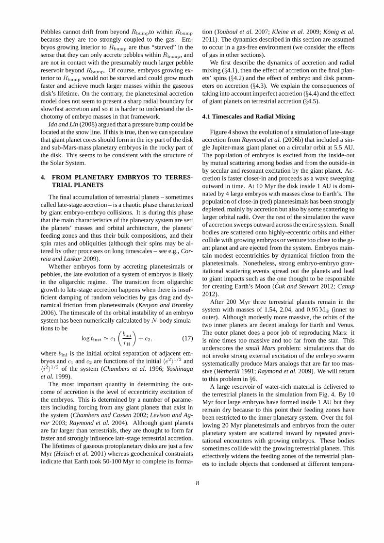
During the late stages of runaway growth, embryos growwhile interacting with one another. The dynamics of thesystem become dominated by a relatively small number –a few tens to a few hundred – oligarchs (Kokubo and Ida1998, 2000;Thommes et al.2003).

Oligarchic growth is the result of the self-limiting natureof runaway growth and orbital repulsion of planetary em-bryos. The formation of similar-sized planetary embryos isdue to a slow-down of runaway growth (Lissauer1987;Idaand Makino1993;Ormel et al.2010). When the mass of aplanetary embryoM exceeds about 100 times that of the av-erage planetesimal, the embryo increases the random veloc-ity of neighboring planetesimals to bev ∝ M1/3 (but notethat this depends on the planetesimal size;Ida and Makino1993;Rafikov2004;Chambers2006). The relative growthrate (from Eq.5) becomes

1

M

dM

dt∝ ΣdustM

−1/3. (7)

Σdust decreases through accretion of planetesimals bythe embryo asM increases (Lissauer 1987). The rel-ative growth rate is a decreasing function ofM , whichchanges the growth mode to orderly. Neighboring embryosgrow while maintaining similar masses. During this stage,the mass ratio of an embryo to its neighboring planetesi-mals increases because for the planetesimals with massm,(1/m)dm/dt ∝ Σdustm

1/3M−2/3, such that

(1/M)dM/dt

(1/m)dm/dt∝

(

M

m

)1/3

. (8)

The relative growth rate of the embryo is by a factor of(M/m)1/3 larger than the planetesimals’. A bi-modalembryo-planetesimal system is formed. While the planetaryembryos grow, a process called orbital repulsion keeps theirorbital separations at roughly 10 mutual Hill radiiRH,m,

where RH,m = 1/2 (a1 + a2) [(M1 + M2)/(3M⋆)]1/3;

here subscripts 1 and 2 refer to adjacent embryos. Orbitalrepulsion is a coupling effect of gravitational scatteringbetween planetary embryos that increases their orbital sep-aration and eccentricities and dynamical friction from smallplanetesimals that decreases the eccentricities (Kokubo andIda 1995). Essentially, if two embryos come too close toeach other their eccentricities are increased by gravitationalperturbations. Dynamical friction from the planetesimalsre-circularizes their orbits at a wider separation.

An example of oligarchic growth is shown in Figure 2(Kokubo and Ida2002). About 10 embryos form withmasses comparable to Mars’ (M ≈ 0.1 M⊕) on nearly cir-cular non-inclined orbits with characteristic orbital separa-tions of10RH,m . At largea the planetary embryos are stillgrowing at the end of the simulation.

Although oligarchic growth describes the accretion ofembryos from planetesimals, it implies giant collisions be-tween embryos that happen relatively early and are fol-lowed by a phase of planetesimal accretion. Consider thelast pairwise accretion of a system of oligarchs on their

5

0.4 0.6 0.8 1 1.2 1.4 1.6

0

0.05

0.1

0.15

Fig. 2.— Oligarchic growth of planetary embryos. Snap-shots of the planetesimal system on thea-e plane are shownfor t = 0, 105, 2 × 105, and4 × 105 years. The circlesrepresent planetesimals with radii proportional to their truevalues. The initial planetesimal system consists of 10000equal-mass (m = 2.5 × 10−4 M⊕) bodies. In this simula-tion, a 6-fold increase in the planetesimal radius was used toaccelerate accretion. In4×105 years, the number of bodiesdecreases to 333. FromKokubo and Ida(2002).

way to becoming planetary embryos. The oligarchs havemassesMolig and are spaced byN mutual Hill radiiRH,m,whereN ≈ 10 is the rough stability limit for such a sys-tem. The final system of embryos will likewise be sep-arated byN RH,m, but with larger massesMemb. Theembryos grow by accreting material within an annulus de-fined by the inter-embryo separation. Assuming pairwisecollisions between equal-mass oligarchs to form a sys-tem of equal-mass embryos, the following simple relationshould hold: NRH,m(M) = 2 N RH,m(Memb). Giventhat RH,m(M) ∼ (2M)1/3, this implies thatMemb =8Molig. After the collision between a pair of oligarchs, eachembryo must therefore accrete the remaining three quartersof its mass from planetesimals.

We can estimate the dynamical properties of a system ofembryos formed by oligarchic growth. We introduce a pro-toplanetary disk with surface density of dust and gasΣdust

andΣgas defined as:

Σdust = ficeΣ1

( a

1 AU

)−x

gcm−2

Σgas = fgasΣ1

( a

1 AU

)−x

gcm−2, (9)

whereΣ1 is simply a reference surface density in solids at1 AU andx is the radial exponent.fice andfgas are factorsthat enhance the surface density of ice and gas with respectto dust. In practicefice is generally taken to be 2-4 (seeKokubo and Ida2002; Lodders2003) andfgas ≈ 100.Given an orbital separationb of embryos, the isolation (fi-nal) mass of a planetary embryo at orbital radiusa is esti-mated as (Kokubo and Ida2002):

Miso ≃ 2πabΣdust = 0.16(

b10rH

)3/2 (

ficeΣ1

10

)3/2

(

a1AU

)(3/2)(2−x)(

M⋆

M⊙

)−1/2

M⊕, (10)

whereM⋆ is the stellar mass. The time evolution of an oli-garchic body is (Thommes et al.2003;Chambers2006):

M(t) = Miso tanh3

(

t

τgrow

)

. (11)

The growth timescaleτgrow is estimated as

τgrow = 1.1 × 106f−1/2ice

(

fgas

240

)−2/5 (

Σ1

10

)−9/10

(

b

10rH

)1/10( a

1 AU

)8/5+9x/10(

M⋆

M⊙

)−8/15

(

ρp

2 gcm−3

)11/15( rp

100 km

)2/5

yr, (12)

whererp andρp are the physical radius and internal densityof planetesimals. Eq. (11) indicates that the embryo gains44%, 90%, and 99% of its final mass during 1τgrow, 2τgrow,and 3τgrow.

For the standard disk model defined above,Miso ∼0.1 M⊕ in the terrestrial planet region. This suggests thatif they formed by oligarchic growth, Mercury and Marsmay simply represent leftover planetary embryos. A shortgrowth timescale (τgrow < 2 Myr) of Mars estimated by theHf-W chronology (Dauphas and Pourmand2011) wouldsuggest that Mars accreted from a massive disk of smallplanetesimals (Kobayashi and Dauphas2013;Morishimaet al. 2013). Alternately, accretion of larger planetesimalsmight have been truncated as proposed by the Grand Tackmodel (see§6.3). Unlike Mars and Mercury, further accre-tion of planetary embryos is necessary to complete Venusand Earth. This next, final stage is called late-stage accre-tion (see Section 4).

3.2 Embryo formation by pebble accretion

Lambrechts and Johansen(2012), hereafter LJ12, pro-posed a new model of growth for planetary embryos and

6

giant planet cores. They argued that if the disk’s massis dominated by pebbles of a few decimeters in size, thelargest planetesimals accrete pebbles very efficiently andcan rapidly grow to several Earth masses (see alsoJohansenand Lacerda2010;Ormel and Klahr2010;Murray-Clayet al. 2011). This model builds on a recent planetesimalformation model in which large planetesimals (with sizesfrom∼ 100 up to∼1,000km) form by the collapse of a self-gravitating clump of pebbles, concentrated to high densitiesby disk turbulence and the streaming instability (Youdin andGoodman2005;Johansen et al.2006, 2007, 2009, see alsochapter by Johansen et al). The pebble accretion scenarioessentially describes how large planetesimals continue toaccrete. There is observational evidence for the existenceofpebble-sized objects in protoplanetary disks (Wilner et al.2005; Rodmann et al.2006; Lommen et al.2007; Perezet al.2012), although their abundance relative to larger ob-jects (planetesimals) is unconstrained.

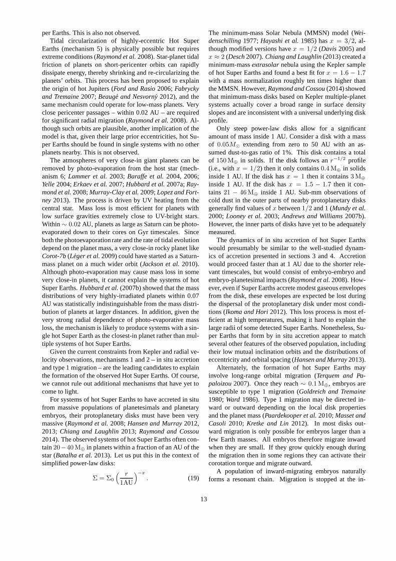
Pebbles are strongly coupled with the gas so they en-counter the already-formed planetesimals with a velocity∆v that is equal to the difference between the Keplerianvelocity and the orbital velocity of the gas, which is slightlysub-Keplerian due to the outward pressure gradient. LJ12define the planetesimalBondi radius as the distance atwhich the planetesimal exerts a deflection of one radian ona particle approaching with a velocity∆v:

RB =GM

∆v2(13)

whereG is the gravitational constant andM is the plan-etesimal mass (the deflection is larger if the particle passescloser thanRB). LJ12 showed that all pebbles with a stop-ping time tf smaller than the Bondi timetB = RB/∆vthat pass within a distanceR = (tf/tB)1/2RB spiral downtowards the planetesimal and are accreted by it. Thus, thegrowth rate of the planetesimal is:

dM/dt = πρR2∆v (14)

whereρ is the volume density of the pebbles in the disk.BecauseR ∝ M , the accretion ratedM/dt ∝ M2. Thus,pebble accretion is at the start a super-runaway process thatis faster than the runaway accretion scenario (see Sec 3.1)in whichdM/dt ∝ M4/3. According to LJ12, this impliesthat in practice, only planetesimals more massive than∼10−4 M⊕ (comparable to Ceres’ mass) undergo significantpebble accretion and can become embryos/cores.

The super-runaway phase cannot last very long. Whenthe Bondi radius exceeds the scale height of the pebblelayer, the accretion rate becomes

dM/dt = 2RΣ∆v (15)

whereΣ is the surface density of the pebbles. This rate isproportional toM , at the boundary between runaway andorderly (oligarchic) growth.

Moreover, when the Bondi radius exceeds the Hill radiusRH = a [M/(3M⋆)]

1/3, the accretion rate becomes

dM/dt = 2RHΣvH (16)

−4 −2 0 2 4x/rB

4

2

0

−2

−4

y/r B

tf=tBtf=100tB

rB

Fig. 3.— Trajectories of particles in the vicinity of a grow-ing embryo. The black curves represent particles stronglycoupled to the gas and the gray curves particles that areweakly coupled, as measured by the ratio of the stoppingtime tf to the Bondi timetB. The orbits of weakly-coupledparticles are deflected by the embryo’s gravity, but thestrongly coupled particles spiral inward and are quickly ac-creted onto the embryo. FromLambrechts and Johansen(2012).

wherevH is the Hill velocity (i.e. the difference in Kep-lerian velocities between two circular orbits separated byRH ). HeredM/dt ∝ M2/3 and pebble accretion enters anoligarchic regime.

For a given surface density of solidsΣ the growth ofan embryo is much faster if the solids are pebble-sizedthan planetesimal sized. This is the main advantage ofthe pebble-accretion model. However, pebble accretionends when the gas disappears from the protoplanetary disk,whereas runaway/oligarchic accretion of planetesimals cancontinue. Also, the ratio betweenΣplanetesimals/Σpebbles

remains to be quantified, and ultimately it is this ratio thatdetermines which accretion mechanism is dominant.

An important problem in Solar System formation is thatthe planetary embryos in the inner solar system are thoughtto have grown only up to at most a Mars-mass, whereas inthe outer solar system some of them reached many Earthmasses, enough to capture a primitive atmosphere and be-come giant planets. The difference between these massescan probably be better understood in the framework of thepebble-accretion model than in the planetesimal-accretionmodel.

The dichotomy in embryo mass in the inner/outer SolarSystem might have been caused by radial drift of pebbles.We consider a disk with a “pressure bump” (Johansen et al.2009) at a given radiusRbump. At this location the gas’azimuthal velocityvθ is larger than the Kepler velocityvK .

7

Pebbles cannot drift from beyondRbumpto within Rbump

because they are too strongly coupled to the gas. Em-bryos growing interior toRbump are thus “starved” in thesense that they can only accrete pebbles withinRbump, andare not in contact with the presumably much larger pebblereservoir beyondRbump. Of course, embryos growing ex-terior toRbump would not be starved and could grow muchfaster and achieve much larger masses within the gaseousdisk’s lifetime. On the contrary, the planetesimal accretionmodel does not seem to present a sharp radial boundary forslow/fast accretion and so it is harder to understand the di-chotomy of embryo masses in that framework.

Ida and Lin(2008) argued that a pressure bump could belocated at the snow line. If this is true, then we can speculatethat giant planet cores should form in the icy part of the diskand sub-Mars-mass planetary embryos in the rocky part ofthe disk. This seems to be consistent with the structure ofthe Solar System.

4. FROM PLANETARY EMBRYOS TO TERRES-TRIAL PLANETS

The final accumulation of terrestrial planets – sometimescalled late-stage accretion – is a chaotic phase characterizedby giant embryo-embryo collisions. It is during this phasethat the main characteristics of the planetary system are set:the planets’ masses and orbital architecture, the planets’feeding zones and thus their bulk compositions, and theirspin rates and obliquities (although their spins may be al-tered by other processes on long timescales – see e.g.,Cor-reia and Laskar2009).

Whether embryos form by accreting planetesimals orpebbles, the late evolution of a system of embryos is likelyin the oligarchic regime. The transition from oligarchicgrowth to late-stage accretion happens when there is insuf-ficient damping of random velocities by gas drag and dy-namical friction from planetesimals (Kenyon and Bromley2006). The timescale of the orbital instability of an embryosystem has been numerically calculated byN -body simula-tions to be

log tinst ≃ c1

(

bini

rH

)

+ c2, (17)

wherebini is the initial orbital separation of adjacent em-bryos andc1 andc2 are functions of the initial〈e2〉1/2 and〈i2〉1/2 of the system (Chambers et al.1996; Yoshinagaet al.1999).

The most important quantity in determining the out-come of accretion is the level of eccentricity excitation ofthe embryos. This is determined by a number of parame-ters including forcing from any giant planets that exist inthe system (Chambers and Cassen2002;Levison and Ag-nor 2003;Raymond et al.2004). Although giant planetsare far larger than terrestrials, they are thought to form farfaster and strongly influence late-stage terrestrial accretion.The lifetimes of gaseous protoplanetary disks are just a fewMyr (Haisch et al.2001) whereas geochemical constraintsindicate that Earth took 50-100 Myr to complete its forma-

tion (Touboul et al.2007;Kleine et al.2009;Konig et al.2011). The dynamics described in this section are assumedto occur in a gas-free environment (we consider the effectsof gas in other sections).

We first describe the dynamics of accretion and radialmixing (§4.1), then the effect of accretion on the final plan-ets’ spins (§4.2) and the effect of embryo and disk param-eters on accretion (§4.3). We explain the consequences oftaking into account imperfect accretion (§4.4) and the effectof giant planets on terrestrial accretion (§4.5).

4.1 Timescales and Radial Mixing

Figure 4 shows the evolution of a simulation of late-stageaccretion fromRaymond et al.(2006b) that included a sin-gle Jupiter-mass giant planet on a circular orbit at 5.5 AU.The population of embryos is excited from the inside-outby mutual scattering among bodies and from the outside-inby secular and resonant excitation by the giant planet. Ac-cretion is faster closer-in and proceeds as a wave sweepingoutward in time. At 10 Myr the disk inside 1 AU is domi-nated by 4 large embryos with masses close to Earth’s. Thepopulation of close-in (red) planetesimals has been stronglydepleted, mainly by accretion but also by some scattering tolarger orbital radii. Over the rest of the simulation the waveof accretion sweeps outward across the entire system. Smallbodies are scattered onto highly-eccentric orbits and eithercollide with growing embryos or venture too close to the gi-ant planet and are ejected from the system. Embryos main-tain modest eccentricities by dynamical friction from theplanetesimals. Nonetheless, strong embryo-embryo grav-itational scattering events spread out the planets and leadto giant impacts such as the one thought to be responsiblefor creating Earth’s Moon (Cuk and Stewart2012;Canup2012).

After 200 Myr three terrestrial planets remain in thesystem with masses of 1.54, 2.04, and0.95 M⊕ (inner toouter). Although modestly more massive, the orbits of thetwo inner planets are decent analogs for Earth and Venus.The outer planet does a poor job of reproducing Mars: itis nine times too massive and too far from the star. Thisunderscores thesmall Marsproblem: simulations that donot invoke strong external excitation of the embryo swarmsystematically produce Mars analogs that are far too mas-sive (Wetherill1991;Raymond et al.2009). We will returnto this problem in§6.

A large reservoir of water-rich material is delivered tothe terrestrial planets in the simulation from Fig. 4. By 10Myr four large embryos have formed inside 1 AU but theyremain dry because to this point their feeding zones havebeen restricted to the inner planetary system. Over the fol-lowing 20 Myr planetesimals and embryos from the outerplanetary system are scattered inward by repeated gravi-tational encounters with growing embryos. These bodiessometimes collide with the growing terrestrial planets. Thiseffectively widens the feeding zones of the terrestrial plan-ets to include objects that condensed at different tempera-

8

0.0

0.2

0.4

0.01 Myr

0.0

0.2

0.4

1 Myr

0.0

0.2

0.4

3 Myr

0.0

0.2

0.4

10 Myr

0.0

0.2

0.4

30 Myr

0 1 2 3 4 50.0

0.2

0.4

200 Myr

Semimajor Axis (AU)

Ecc

entr

icity

Log(Water Mass Fraction)

-5 -4 -3 -2 -1.3

Fig. 4.— Six snapshots of a simulation of terrestrial planet for-mation (adapted fromRaymond et al.2006b). The simulationstarted from 1885 self-gravitating sub-lunar-mass bodiesspreadfrom 0.5 to 5 AU following anr

−3/2 surface density profile,comprising a total of9.9 M⊕. The large black circle representsa Jupiter-mass planet. The size of each body is proportionaltoits mass1/3. The color represents each body’s water content (seecolor bar).

tures and therefore have different initial compositions (seealsoBond et al.2010;Carter-Bond et al.2012;Elser et al.2012). The compositions of the terrestrial planets becomemixtures of the compositions of their constituent embryosand planetesimals. The planets’ feeding zones representthose constituents. When objects from past 2.5 AU are ac-creted, water-rich material is delivered to the planet in theform of hydrated embryos and planetesimals. In the simu-lations, from 30-200 Myr the terrestrial planets accrete ob-jects from a wide range of initial locations and are deliveredmore water.

Given that the water delivered to the planets in this sim-ulation originated in the region between 2.5 and 4 AU, itscomposition should be represented by carbonaceous chon-drites, which provide a very good match to Earth’s wa-ter (Morbidelli et al. 2000;Marty and Yokochi2006). Theplanets are delivered a volume of water that may be toolarge. For example, the Earth analog’s final water contentby mass was8× 10−3, roughly 8-20 times the actual value.However, water loss during giant impacts was not taken intoaccount in the simulation (see, e.g.,Genda and Abe2005).

4.2 Planetary spins

Giant impacts impart large amounts of spin angular mo-mentum on the terrestrial planets (e.g.,Safronov1969;Lis-sauer and Kary1991;Dones and Tremaine1993). The last

few giant impacts tend to dominate the spin angular mo-mentum (Agnor et al.1999;Kokubo and Ida2007;Kokuboand Genda2010). Using a “realistic” accretion condition ofplanetary embryos (Genda et al.2012, see§4.4)),Kokuboand Genda(2010) found that the spin angular velocity ofaccreted terrestrial planets follows a Gaussian distributionwith a nearly mass-independent average value of about 70%of the critical angular velocity for rotational breakup

ωcr =

(

GM

R3

)1/2

, (18)

whereM andR are the mass and radius of a planet. Thisappears to be a natural outcome of embryo-embryo impactsat speeds slightly larger than escape velocity. At later times,during the late veneer phase, the terrestrial planets’ spinsare further affected by impacts with planetesimals (Ray-mond et al.2013).

The obliquity of accreted planets ranges from 0◦ to 180◦

and follows an isotropic distribution (Agnor et al.1999;Kokubo and Ida2007; Kokubo and Genda2010). Bothprograde and retrograde spins are equally probable. Theisotropic distribution ofε is a natural outcome of giant im-pacts. During the giant impact stage, the thickness of aplanetary embryo system is∼ a〈i2〉1/2 ∼ 10rH, far largerthan the radiusR of planetary embryosR ∼ 10−2rH, wherea, i, andrH are the semimajor axis, inclination and Hill ra-dius of planetary embryos. Thus, collisions are fully three-dimensional and isotropic, which leads to isotropic spin an-gular momentum. This result clearly shows that progradespin with small obliquity, which is common to the terres-trial planets in the solar system except for Venus, is nota common feature for planets assembled by giant impacts.Note that the initial obliquity of a planet determined by gi-ant impacts can be modified substantially by stellar tide ifthe planet is close to the star and by satellite tide if the planethas a large satellite.

4.3 Effect of disk and embryo parameters

The properties of a system of terrestrial planets areshaped in large part by the total mass and mass distributionwithin the disk, and the physical and orbital properties ofplanetary embryos and planetesimals within the disk. How-ever, while certain parameters have a strong impact on theoutcome, others have little to no effect.

Kokubo et al.(2006) performed a suite of simulations ofaccretion of populations of planetary embryos to test the im-portance of the embryo density, mass, spacing and number.They found that the bulk density of the embryos had little tono effect on the accretion within the range that they tested,ρ = 3.0 − 5.5g cm−3. One can imagine that the dynam-ics could be affected for extremely high values ofρ, if theescape speed from embryos were to approach a significantfraction of the escape speed from the planetary system (Gol-dreich et al.2004). In practice this is unlikely to occur inthe terrestrial planet forming region because it would re-

9

quire unphysically-large densities. The initial spacing like-wise had no meaningful impact on the outcome, at leastwhen planetary embryos were spaced by 6-12 mutual Hillradii (Kokubo et al.2006). Likewise, for a fixed total massin embryos, the embryo mass was not important.

The total mass in embryos does affect the outcome.A more massive disk of embryos and planetesimals pro-duces fewer, more massive planets than a less massivedisk (Kokubo et al.2006; Raymond et al.2007a). Em-bryos’ eccentricities are excited more strongly in massivedisks by encounters with massive embryos. With largermean eccentricities, the planets’ feeding zones are widerthan if the embryos’ eccentricities were small, simply be-cause any given embryos crosses a wider range of orbitalradii. The scaling between the mean accreted planet massand the disk mass is therefore slightly steeper than linear:the mean planet massMp scales with the local surface den-sity Σ0 asMp ∝ Σ1.1

0 (Kokubo et al.2006). It is interestingto note that this scaling is somewhat shallower than theΣ1.5

0

scaling of embryo mass with the disk mass (Kokubo and Ida2000). Accretion also proceeds faster in high-mass disks, asthe timescale for interaction drops.

Terrestrial planets that grow from a disk of planetesimalsand planetary embryos retain a memory of the surface den-sity profile of their parent disk. In addition, the dynamics isinfluenced by which part of the disk contains the most mass.In disks with steep density profiles – i.e., if the surface den-sity scales with orbital radius asΣ ∝ r−x, disks with largevalues ofx – more mass is concentrated in the inner parts ofthe disk, where the accretion times are faster and protoplan-ets are dry. Compared with disks with shallower densityprofiles (with smallx), in disks with steep profiles the ter-restrial planets tend to be more massive, form more quickly,form closer-in, and contain less water (Raymond et al.2005;Kokubo et al.2006).

4.4 Effect of imperfect accretion

As planetesimals eccentricities are excited by growingembryos, they undergo considerable collisional grinding.Collisional disruption can be divided into two types: catas-trophic disruption due to high-energy impacts and crater-ing due to low-energy impacts.Kobayashi and Tanaka(2010a) found that cratering collisions are much more ef-fective in collisional grinding than collisions causing catas-trophic disruption, simply because the former impacts occurmuch more frequently than the latter ones. Small fragmentsare easily accreted by embryos in the presence of nebu-lar gas (Wetherill and Stewart1993), although they rapidlydrift inward due to strong gas drag, leading to small embryomasses (Chambers2008;Kobayashi and Tanaka2010b).

Giant impacts between planetary embryos often do notresult in net accretion. Rather, there exists a diversity ofcollisional outcomes. These include near-perfect mergingat low impact speeds and near head-on configurations, par-tial accretion at somewhat higher impact speeds and angles,“hit and run” collisions at near-grazing angles, and even net

erosion for high-speed, near head-on collisions (Agnor andAsphaug2004;Asphaug et al.2006;Asphaug2010). Tworecent studies used large suites of SPH simulations to mapout the conditions required for accretion in the parameterspace of large impacts (Genda et al.2012;Leinhardt andStewart2012). However, mostN -body simulations of ter-restrial planet formation to date have assumed perfect ac-cretion in which all collisions lead to accretion.

About half of the embryo-embryo impacts in a typi-cal simulation of late-stage accretion do not lead to netgrowth (Agnor and Asphaug2004; Kokubo and Genda2010). Rather, the outcomes are dominated by partially ac-creting collision, hit-and-run impacts, and graze-and-mergeevents in which two embryos dissipate sufficient energyduring a grazing impact to become gravitationally boundand collide (Leinhardt and Stewart2012).

Taking into account only the accretion condition forembryo-embryo impacts, the final number, mass, orbital el-ements, and even growth timescale of planets are barelyaffected (Kokubo and Genda2010;Alexander and Agnor1998). This is because even though collisions do not lead toaccretion, the colliding bodies stay on the colliding orbitsafter the collision and thus the system is unstable and thenext collision occurs shortly.

However, by allowing non-accretionary impacts to botherode the target embryo and to produce debris particles,Chambers(2013) found that fragmentation does have anoted effect on accretion. The final stages of accretion arelengthened by the sweep up of collisional fragments. Theplanets that formed in simulations with fragmentation hadsmaller masses and smaller eccentricities than their coun-terparts in simulations without fragmentation.

Imperfect accretion also affects the planets’ spin rates.Kokubo and Genda(2010) found that the spin angular mo-mentum of accreted planets was 30% smaller than in simu-lations with perfect accretion. This is because grazing col-lisions that have high angular momentum are likely to re-sult in a hit-and-run, while nearly head-on collisions thathave small angular momentum lead to accretion. The pro-duction of unbound collisional fragments with high angu-lar momentum could further reduce the spin angular veloc-ity. The effect of non-accretionary impacts on the planetaryspins has yet to be carefully studied.

A final consequence of fragmentation is on the core massfraction. Giant impacts lead to an increase in the core massfraction because the mantle is preferentially lost during im-perfect merging events (Benz et al.2007;Stewart and Lein-hardt 2012;Genda et al.2012). However, the sweep-upof these collisional fragments on 100 Myr timescales re-balances the composition of planets to roughly the initialembryo composition (Chambers2013). We speculate that anet increase in core mass fraction should be retained if therocky fragments are allowed to collisionally evolve and losemass.

4.5 Effect of outer giant planets

10

We now consider the effect of giant planets on terrestrialaccretion. We restrict ourselves to systems with giant plan-ets similar to our own Jupiter and Saturn. That is, systemswith non-migrating giant planets on stable orbits exteriortothe terrestrial planet-forming region. In§5.2 we will con-sider the effects of giant planet migration and planet-planetscattering.

The most important effect of giant planets on terrestrialaccretion is the excitation of the eccentricities of plane-tary embryos. This generally occurs by the giant planet-embryo gravitational eccentricity forcing followed by thetransmission of that forcing by embryo-embryo or embryo-planetesimal forcing. The giant planet forcing typicallyoccurs via mean motion or secular resonances, or secu-lar dynamical forcing. Giant planet-embryo excitation isparticularly sensitive to the giant planets’ orbital architec-ture (Chambers and Cassen2002;Levison and Agnor2003;Raymond2006). Figure 5 shows the eccentricities of testparticles excited for 1 Myr by two different configurationsof Jupiter and Saturn (Raymond et al.2009), both of whichare consistent with the present-day Solar System (see§6).The spikes in eccentricity seen in Fig. 5 come from specificresonances: in theJSRESconfiguration (for “Jupiter andSaturn in RESonance”), theν5 secular resonance at 1.3 AUand the 2:1 mean motion resonance with Jupiter at 3.4 AU;and in theEEJSconfiguration (for “Extra-Eccentric Jupiterand Saturn”) theν5 andν6 secular resonances at 0.7 and2.1 AU, and a hint of the 2:1 mean motion resonance withJupiter at 3.3 AU. The “background” level of excitation seenin Fig. 5 comes from secular forcing, following a smoothfunction of the orbital radius.

The eccentricity excitation of terrestrial embryos is sig-nificant even for modest values of the giant planets’ ec-centricity. In Fig. 5, Jupiter and Saturn have eccentricitiesof 0.01-0.02 in theJSRESconfiguration and of 0.1 in theEEJSconfiguration. The test particles in theJSRESsys-tem are barely excited by the giant planets interior to 3 AU;the magnitude of the spike at 1.3 AU is far smaller thanthe secular forcing anywhere in theEEJSsimulation. Notealso that this figure represents just the first link in the chain.The eccentricities imparted to embryos are systematicallytransmitted to the entire embryo swarm, and it is the meaneccentricity of the embryo swarm that dictates the outcomeof accretion.

In a population of embryos with near-circular orbits, thecommunication zone – the radial distance across which agiven embryo has gravitational contact with its neighbors –is very narrow. Embryos grow by collisions with their im-mediate neighbors. The planets that form are thus limited inmass by the mass in their immediate vicinity. In contrast, ina population of embryos with significant eccentricities, thecommunication zone of embryos is wider. Each embryo’sorbit crosses the orbits of multiple other bodies and, by sec-ular forcing, gravitationally affects the orbits of even more.This of course does not imply any imminent collisions, butit does mean that the planets that form will sample a widerradial range of the disk than in the case of very low embryo

eccentricities. This naturally produces a smaller number ofmore massive planets. Given that collisions preferentiallyoccur at pericenter, the terrestrial planets that form tendtoalso be located closer-in when the mean embryo eccentric-ity is larger (Levison and Agnor2003).

In systems with one or more giant planets on orbits ex-terior to the terrestrial planet-forming region, the amplitudeof excitation of the eccentricities of terrestrial embryosislarger when the giant planets’ orbits are eccentric or closer-in. The timescale for excitation is shorter when the giantplanets are more massive. Thus, the strongest perturbationscome from massive eccentric gas giants.

Simulations have indeed shown that systems with mas-sive or eccentric outer gas giants systematically producefewer, more massive terrestrial planets (Chambers andCassen2002; Levison and Agnor2003; Raymond et al.2004). However, the efficiency of terrestrial accretion issmaller in the presence of a massive or eccentric gas giantbecause a fraction of embryos and planetesimals are excitedonto orbits that are unstable and are thus removed from thesystem. The most common mechanism for the removal ofsuch bodies is by having their eccentricities increased tothe point where their orbits cross those of a giant planet,then being ejected entirely from the system into interstellarspace.

The strong outside-in perturbations produced by massiveor eccentric outer gas giants also act to accelerate terres-trial planet formation. This happens for two reasons. First,when embryos have significant mean eccentricities the typ-ical time between encounters decreases, as long as eccen-tricities are more strongly perturbed than inclinations. Sec-ond, accretion is slower in the outer parts of planetary sys-tems because of the longer orbital and encounter timescales,and it is these slow-growing regions that are most efficientlycleared by the giant planets’ perturbations.

Given their outside-in influence, outer gas giants alsoplay a key role in water delivery to terrestrial planets. Itshould be noted up front that the gas giants’ role in waterdelivery is purely detrimental, at least in the context of outergiant planets on static orbits. Stimulating the eccentricitiesof water-rich embryos at a few AU can in theory cause someembryos to be scattered inward and deliver water to the ter-restrial planets. In practice, a much larger fraction of bod-ies is scattered outward, encounters the giant planets and isejected from the system than is scattered inward to deliverwater (Raymond et al.2006b).

Finally, simulations with setups similar to the one fromFig. 4 confirm that the presence of one or more giant planetsstrongly anti-correlates with the water content of the terres-trial planets in those systems (Chambers and Cassen2002;Raymond et al.2004, 2006b, 2007b, 2009;O’Brien et al.2006). There is a critical orbital radius beyond which a gi-ant planet must lie for terrestrial planets to accrete and sur-vive in a star’s liquid water habitable zone (Raymond2006).This limit is eccentricity dependent: a zero-eccentricity(single) giant planet must lie beyond 2.5 AU to allow a ter-restrial planet to form between 0.8 and 1.5 AU whereas a

11

Fig. 5.— Excitation of test particles by two configurations of Jupiter and Saturn. Each panel shows the eccentricities of masslesstest particles after 1 Myr (giant planets not shown). Note the difference in the y-axis scale between the two panels. Eachscenario isconsistent with the present-day Solar System (see discussion in§6). Jupiter and Saturn are in 3:2 mean motion resonance with semimajoraxes of 5.4 and 7.2 AU and low eccentricities in theJSRESconfiguration. The gas giants are at their current semimajoraxes of 5.2 and9.5 AU with eccentricities of 0.1 in theEEJSconfiguration. FromRaymond et al.(2009).

giant planet with an eccentricity of 0.3 must lie beyond 4.2AU. For water to be delivered to the terrestrial planets froma presumed source at 2-4 AU (as in Fig. 4) the giant planetmust be farther still (Raymond2006).

5. TERRESTRIAL ACCRETION IN EXTRA-SOLARPLANETARY SYSTEMS

Extra-solar planetary systems do not typically look likethe Solar System. To extrapolate to extra-solar planetarysystems is therefore not trivial. Additional mechanismsmust be taken into account, in particular orbital migrationboth of planetary embryos (Type 1 migration) and of gasgiant planets (Type 2 migration) and dynamical instabilitiesin systems of multiple gas giant planets.

There exists ample evidence that accretion does indeedoccur around other stars. Not only has an abundance oflow-mass planets been detected (Mayor et al.2011;Batalhaet al. 2013), but the dust produced during terrestrial planetformation (Kenyon and Bromley2004) has also been de-tected (e.g.Meyer et al.2008;Lisse et al.2008), includ-ing the potential debris from giant embryo-embryo im-pacts (Lisse et al.2009).

In this section we first address the issue of the forma-tion of hot Super Earths. Then we discuss how the dynam-ics shaping the known systems of giant planets may havesculpted unseen terrestrial planets in those systems.

5.1 Hot Super Earths

Hot Super Earths are extremely common. Roughly onethird to one half of Sun-like (FGK) stars host at least oneplanet with a mass less than10 M⊕ and a period of lessthan50−100 days (Howard et al.2010;Mayor et al.2011).The frequency of Hot Super Earths is at least as high aroundM stars as around FGK stars and possibly higher (Howardet al. 2012;Bonfils et al.2013;Fressin et al.2013). HotSuper Earths are typically found in systems of many planets

on compact but non-resonant orbits (e.g.Udry et al.2007;Lovis et al.2011;Lissauer et al.2011).

Several mechanisms have been proposed to explain theorigin of Hot Super Earths (seeRaymond et al.2008): 1)In situ accretion from massive disks of planetary embryosand planetesimals; 2) Accretion during inward type 1 mi-gration of planetary embryos; 3) Shepherding in interiormean motion resonances with inward-migrating gas giantplanets; 4) Shepherding by inward-migrating secular res-onances driven by dissipation of the gaseous disk; 5) Cir-cularization of planets on highly-eccentric orbits by star-planet tidal interactions; 6) Photo-evaporation of close-ingas giant planets.

Theoretical and observational constraints effectively ruleout mechanisms 3-6. The shepherding of embryos bymigrating resonances (mechanisms 3 and 4) can robustlytransport material inward (Zhou et al.2005;Fogg and Nel-son2005, 2007;Raymond et al.2006a;Mandell et al.2007;Gaidos et al.2007). An embryo that finds itself in reso-nance with a migrating giant planet will have its eccentricitysimultaneously excited by the giant planet and damped bytidal interactions with the gaseous disk (Tanaka and Ward2004; Cresswell et al.2007). As the tidal damping pro-cess is non-conservative, the embryo’s orbit loses energyand shrinks, removing the embryo from the resonance. Themigrating resonance catches up to the embryo and the pro-cess repeats itself, moving the embryo inward, potentiallyacross large distances. This mechanism is powered by themigration of a strong resonance. This requires a connec-tion between Hot Super Earths and giant planets. If a giantplanet migrated inward, and the shepherd was a mean mo-tion resonance (likely the 3:2, 2:1 or 3:1 resonance) thenhot Super Earths should be found just interior to close-ingiant planets, which is not observed. If a strong secularresonance migrated inward then at least one giant planeton an eccentric orbit must exist exterior to the hot SuperEarth, and there should only be a small number of Hot Su-

12

per Earths. This is also not observed.Tidal circularization of highly-eccentric Hot Super

Earths (mechanism 5) is physically possible but requiresextreme conditions (Raymond et al.2008). Star-planet tidalfriction of planets on short-pericenter orbits can rapidlydissipate energy, thereby shrinking and re-circularizingtheplanets’ orbits. This process has been proposed to explainthe origin of hot Jupiters (Ford and Rasio2006;Fabryckyand Tremaine2007;Beauge and Nesvorny 2012), and thesame mechanism could operate for low-mass planets. Veryclose pericenter passages – within 0.02 AU – are requiredfor significant radial migration (Raymond et al.2008). Al-though such orbits are plausible, another implication of themodel is that, given their large prior eccentricities, hot Su-per Earths should be found in single systems with no otherplanets nearby. This is not observed.

The atmospheres of very close-in giant planets can beremoved by photo-evaporation from the host star (mech-anism 6;Lammer et al.2003;Baraffe et al.2004, 2006;Yelle2004;Erkaev et al.2007;Hubbard et al.2007a;Ray-mond et al.2008;Murray-Clay et al.2009;Lopez and Fort-ney2013). The process is driven by UV heating from thecentral star. Mass loss is most efficient for planets withlow surface gravities extremely close to UV-bright stars.Within ∼ 0.02 AU, planets as large as Saturn can be photo-evaporated down to their cores on Gyr timescales. Sinceboth the photoevaporation rate and the rate of tidal evolutiondepend on the planet mass, a very close-in rocky planet likeCorot-7b(Leger et al.2009) could have started as a Saturn-mass planet on a much wider orbit (Jackson et al.2010).Although photo-evaporation may cause mass loss in somevery close-in planets, it cannot explain the systems of hotSuper Earths.Hubbard et al.(2007b) showed that the massdistributions of very highly-irradiated planets within 0.07AU was statistically indistinguishable from the mass distri-bution of planets at larger distances. In addition, given thevery strong radial dependence of photo-evaporative massloss, the mechanism is likely to produce systems with a sin-gle hot Super Earth as the closest-in planet rather than mul-tiple systems of hot Super Earths.

Given the current constraints from Kepler and radial ve-locity observations, mechanisms 1 and 2 – in situ accretionand type 1 migration – are the leading candidates to explainthe formation of the observed Hot Super Earths. Of course,we cannot rule out additional mechanisms that have yet tocome to light.

For systems of hot Super Earths to have accreted in situfrom massive populations of planetesimals and planetaryembryos, their protoplanetary disks must have been verymassive (Raymond et al.2008;Hansen and Murray2012,2013; Chiang and Laughlin2013; Raymond and Cossou2014). The observed systems of hot Super Earths often con-tain20−40 M⊕ in planets within a fraction of an AU of thestar (Batalha et al.2013). Let us put this in the context ofsimplified power-law disks:

Σ = Σ0

( r

1AU

)−x

. (19)

The minimum-mass Solar Nebula (MMSN) model (Wei-denschilling1977;Hayashi et al.1985) hasx = 3/2, al-though modified versions havex = 1/2 (Davis2005) andx ≈ 2 (Desch2007).Chiang and Laughlin(2013) created aminimum-massextrasolarnebula using the Kepler sampleof hot Super Earths and found a best fit forx = 1.6 − 1.7with a mass normalization roughly ten times higher thanthe MMSN. However,Raymond and Cossou(2014) showedthat minimum-mass disks based on Kepler multiple-planetsystems actually cover a broad range in surface densityslopes and are inconsistent with a universal underlying diskprofile.

Only steep power-law disks allow for a significantamount of mass inside 1 AU. Consider a disk with a massof 0.05M⊙ extending from zero to 50 AU with an as-sumed dust-to-gas ratio of 1%. This disk contains a totalof 150 M⊕ in solids. If the disk follows anr−1/2 profile(i.e., with x = 1/2) then it only contains0.4 M⊕ in solidsinside 1 AU. If the disk hasx = 1 then it contains3 M⊕

inside 1 AU. If the disk hasx = 1.5 − 1.7 then it con-tains 21 − 46 M⊕ inside 1 AU. Sub-mm observations ofcold dust in the outer parts of nearby protoplanetary disksgenerally find values ofx between1/2 and 1 (Mundy et al.2000;Looney et al.2003;Andrews and Williams2007b).However, the inner parts of disks have yet to be adequatelymeasured.

The dynamics of in situ accretion of hot Super Earthswould presumably be similar to the well-studied dynam-ics of accretion presented in sections 3 and 4. Accretionwould proceed faster than at 1 AU due to the shorter rele-vant timescales, but would consist of embryo-embryo andembryo-planetesimal impacts (Raymond et al.2008). How-ever, even if Super Earths accrete modest gaseous envelopesfrom the disk, these envelopes are expected be lost duringthe dispersal of the protoplanetary disk under most condi-tions (Ikoma and Hori2012). This loss process is most ef-ficient at high temperatures, making it hard to explain thelarge radii of some detected Super Earths. Nonetheless, Su-per Earths that form by in situ accretion appear to matchseveral other features of the observed population, includingtheir low mutual inclination orbits and the distributions ofeccentricity and orbital spacing (Hansen and Murray2013).

Alternately, the formation of hot Super Earths mayinvolve long-range orbital migration (Terquem and Pa-paloizou2007). Once they reach∼ 0.1 M⊕, embryos aresusceptible to type 1 migration (Goldreich and Tremaine1980;Ward 1986). Type 1 migration may be directed in-ward or outward depending on the local disk propertiesand the planet mass (Paardekooper et al.2010;Masset andCasoli 2010; Kretke and Lin2012). In most disks out-ward migration is only possible for embryos larger than afew Earth masses. All embryos therefore migrate inwardwhen they are small. If they grow quickly enough duringthe migration then in some regions they can activate theircorotation torque and migrate outward.

A population of inward-migrating embryos naturallyforms a resonant chain. Migration is stopped at the in-

13

0.1

1

10Sem

i-m

ajo

r axis

[A

U]

0 0.5 1.0 1.5Time [million years]

02468

10121416

mass [

Eart

hs]

Most massive

2nd most massive

3rd most massive

0 0.5 1.0 1.5Time [million years]

Collisions

0.10 0.15 0.20 0.25 0.30 0.35 0.40 0.45

a [AU]

0

Kepler-11

Simulation

4:3 4:33:2

Fig. 6.— Formation of a system of hot Super Earths by type1 migration. The top panel shows the evolution of the embryos’orbital radii and the bottom panel shows the mass growth. Thered,green and blue curves represent embryos that coagulated into thethree most massive planets. All other bodies are in black. Only themost massive (red) planet grew large enough to trigger outwardmigration before crossing into a zone of pure inward migration.FromCossou et al.(2013).

ner edge of the disk (Masset et al.2006) and the resonantchain piles up against the edge (Ogihara and Ida2009).If the resonant chain gets too long, cumulative perturba-tions from the embryos act to destabilize the chain, lead-ing to accretionary collisions and a new shorter resonantchain (Morbidelli et al.2008;Cresswell and Nelson2008).This process can continue throughout the lifetime of thegaseous disk and include multiple generations of inward-migrating embryos or populations of embryos.

Figure 6 shows the formation of a system of hot SuperEarths by type 1 migration fromCossou et al.(2013). Inthis simulation60 M⊕ in embryos with masses of0.1 −2 M⊕ started from 2-15 AU. The embryos accreted as theymigrated inward in successive waves. One embryo (shownin red in Fig. 6) grew large enough to trigger outward migra-tion and stabilized at a zero-torque zone in the outer disk,presumably to become giant planet core. The system ofhot Super Earths that formed is similar in mass and spacingto the Kepler-11 system (Lissauer et al.2011). The fourouter super Earths are in a resonant chain but the inner onewas pushed interior to the inner edge of the gas disk andremoved from resonance.

It was proposed byRaymond et al.(2008) that transitmeasurements of hot Super Earths could differentiate be-tween the in situ accretion and type 1 migration models.

They argued that planets formed in situ should be nakedhigh-density rocks whereas migrated planets are morelikely to be dominated by low-density material such as ice.It has been claimed that planets that accrete in situ can havethick gaseous envelopes and thus inflated radii (Hansen andMurray 2012;Chiang and Laughlin2013). However, de-tailed atmospheric calculations byIkoma and Hori(2012)suggest that it is likely that low-mass planets generally losetheir atmospheres during disk dispersal. This is a key point.If these planets can indeed retain thick atmospheres thensimple measurements of the bulk density of Super Earthswold not provide a mechanism for differentiation betweenthe models. However, if hot Super Earths cannot retainthick atmospheres after forming in situ, then low densityplanets must have formed at larger orbital distances andmigrated inward.

It is possible that migration and in situ accretion bothoperate to reproduce the observed hot Super Earths. Themain shortcoming of in situ accretion model is that the req-uisite inner disk masses are extremely large and do not fitthe surface density profiles measured in the outskirts of pro-toplanetary disks. Type 1 migration of planetary embryosprovides a natural way to concentrate solids in the innerparts of protoplanetary disks. One can envision a scenariothat proceeds as follows. Embryos start to accrete locallythroughout the disk. Any embryo that grows larger thanroughly a Mars mass type 1 migrates inward. Most em-bryos migrate all the way to the inner edge of the disk, or atleast to the pileup of embryos bordering on the inner edge.There are frequent close encounters and impacts betweenembryos. The embryos form long resonant chains that aresuccessively broken by perturbations from other embryosor by stochastic forcing from disk turbulence (Terquem andPapaloizou2007;Pierens and Raymond2011). As the diskdissipates the resonant chain can be broken, leading to a lastphase of collisions that effectively mimics the in situ accre-tion model. There remains sufficient gas and collisional de-bris to damp the inclinations of the surviving Super Earthsto values small enough to be consistent with observations.However, that it is possible that many Super Earths actuallyremain in resonant orbits but with period ratios altered bytidal dissipation (Batygin and Morbidelli2013).

5.2 Sculpting by giant planets: type 2 migration and dy-namical instabilities

The orbital distribution of giant exoplanets is thought tohave been sculpted by two dynamical processes: type 2 mi-gration and planet-planet scattering (Moorhead and Adams2005;Armitage2007). These processes each involve long-range radial shifts in giant planets’ orbits and have strongconsequences for terrestrial planet formation in those sys-tems. In fact, each of these processes has been proposed toexplain the origin of hot Jupiters (Lin et al.1996;Nagasawaet al. 2008), so differences in the populations of terrestrialplanets, once observed, could help resolve the question ofthe origin of hot Jupiters.

14

Only a fraction of planetary systems contain giant plan-ets. About 14% of Sun-like stars host a gas giant with pe-riod shorter than 1000 days (Mayor et al.2011), althoughthe fraction of stars with more distant giant planets could besignificantly higher (Gould et al.2010).

When a giant planet becomes massive enough to opena gap in the protoplanetary disk, its orbital evolution be-comes linked to the radial viscous evolution of the gas.This is called Type 2 migration (Lin and Papaloizou1986;Ward1997). As a giant planet migrates inward it encountersother small bodies in various stages of accretion. Given thestrong damping of eccentricities by the gaseous disk, a sig-nificant fraction of the material interior to the giant planet’sinitial orbit is shepherded inward by strong resonances asexplained in§5.1 (Zhou et al.2005;Fogg and Nelson2005,2007, 2009;Raymond et al.2006a;Mandell et al.2007). In-deed, the simulation from the left panel of Figure 7 formedtwo hot Super Earth planets, one just interior to the 2:1 and3:1 resonance. The orbits of the two planets became desta-bilized after several Myr, collided and fused into a single4 M⊕ hot Super Earth. There also exists a population ofvery close-in planetesimals in the simulation from Fig. 7;these were produced by the same shepherding mechanismas the hot Super Earths but, because the dissipative forcesfrom gas drag were so much stronger for these objects thanthe damping due to disk-planet tidal interactions felt by theembryos (Adachi et al.1976; Ida et al. 2008), they wereshepherded by a much higher-order resonance, here the 8:1.

Planetesimals or embryos that come too close to the mi-grating giant are scattered outward onto eccentric orbits.These orbits are slowly re-circularized by gas drag and dy-namical friction. On 10-100 Myr or longer timescales asecond generation of terrestrial planets can form from thisscattered material (Raymond et al.2006a;Mandell et al.2007). The building blocks of this new generation of plan-ets are significantly different than the original ones. Thisnew distribution is comprised of two components: bodiesthat originated across the inner planetary system that werescattered outward by the migrating gas giant, and bodiesthat originated exterior to the gas giant. When taking intoaccount the original location of these protoplanets, the ef-fective feeding zone of the new terrestrial planets essen-tially spans the entire planetary system. This new gener-ation of terrestrial planets therefore inevitably contains ma-terial that condensed at a wide range of orbital distances.Their volatile contents are huge. Indeed, the water contentof the 3 M⊕ planet that formed at 0.9 AU (in the shadedhabitable zone) in Fig. 7 is roughly 10% by mass. Even if90% of the water were lost during accretion, that still corre-sponds to ten times Earth’s water content (by mass), mean-ing that this planet is likely to be covered in global oceans.

The simulation from Fig. 7 showed the simple case of asingle giant planet on a low-eccentricity (e ≈ 0.05) migrat-ing through a disk of growing planetesimals and embryos.Migration would be more destructive to planet formationunder certain circumstances. For example, if migration oc-curs very late in the evolution of the disk then less gas re-

mains to damp the eccentricities of scattered bodies. Thisis probably more of an issue for the formation of hot Su-per Earths than for scattered embryos: since the viscoustimescale is shorter closer-in, much of the inner disk may infact drain onto the star during type 2 migration (Thommeset al. 2008) and reduce the efficiency of the shepherdingmechanism. In addition, multiple giant planets may oftenmigrate inward together. In that case the giant planets’ ec-centricities would likely be excited to modest values, andany embryo scattered outward would likely encounter an-other giant planet, increasing the probability of very strongscattering events onto unbound orbits.

Although type 2 migration certainly does not provide acomfortable environment for terrestrial accretion, planet-planet scattering is far more disruptive. The broad eccen-tricity distribution of observed giant exoplanets is natu-rally reproduced if at least 75% of the observed planets arethe survivors of violent dynamical instabilities (Chatterjeeet al.2008;Juric and Tremaine2008;Raymond et al.2010).It is thought that giant planets form in multiple systemson near-circular orbits but in time, perturbations destabi-lize these systems and lead to a phase of close gravitationalencounters. Repeated planet-planet scattering usually leadsto the ejection of one or more giant planets (Rasio and Ford1996;Weidenschilling and Marzari1996, ; see chapter byDavies et al). The large eccentricities of the observed plan-ets are essentially the scars of past instabilities.

Instabilities are also destructive for terrestrial planets ortheir building blocks. The timing of instabilities is poorly-constrained, although it is thought that many instabilitiesmay be triggered by either migration in systems of mul-tiple gas giants (Adams and Laughlin2003;Moorhead andAdams2005) or by the removal of damping during the dissi-pation of the gaseous disk (Moeckel et al.2008;Matsumuraet al. 2010; Moeckel and Armitage2012). On the otherhand, systems of planets on more widely-spaced orbits orsystems with wide binary companions may naturally ex-perience instabilities on Gyr timescales (Marzari and Wei-denschilling2002;Kaib et al. 2013). Although early in-stabilities may allow for additional sources of damping viagas drag from remaining gas and dynamical friction fromabundant planetesimals, in practice the timing of the insta-bility makes little difference for the survival of terrestrialbodies (Raymond et al.2012).

Instabilities between Jupiter-sized planets typically onlylast for∼ 105 years. When a giant planet is scattered onto ahighly-eccentric orbit, even if it only lasts for a relativelyshort time, very strong secular forcing can drive the or-bits of inner terrestrial bodies to very high eccentricities.The outcome of the perturbation is extremely sensitive tothe proximity of the giant planet to the terrestrial planetzone: giant planets whose pericenter distances come withina given separation act so strongly that terrestrial planetsorembryos are driven entirely into the central star (Veras andArmitage2005, 2006;Raymond et al.2011, 2012). Thegiant planet instabilities that are the least disruptive totheterrestrial planets are those that are very short in duration,

15

0.0

0.4

0.8 0.01 Myr

0.0

0.4

0.8 0.04 Myr

0.0

0.4

0.8 0.07 Myr

0.0

0.4

0.8 1 Myr

0.0

0.4

0.8 30 Myr

0.1 1.0 10.00.0

0.4

0.8 200 Myr

Semimajor Axis (AU)

Ecc

entr

icity

Log(Water Mass Fraction)

-5 -4 -3 -2 -1 -0.3

0.0

0.4

0.8 0.01 Myr

0.0

0.4

0.8 1 Myr

0.0

0.4

0.8 10 Myr

0.0

0.4

0.8 42.9 Myr

0.0

0.4

0.8 43.2 Myr

0 2 4 6 8 10 12 14 16 18 20 22 24 26 28 300.0

0.4

0.8 200 Myr

Semimajor Axis (AU)

Ecc

entr

icity

Log(Water Mass Fraction)

-5 -4 -3 -2 -1 -0.3

Fig. 7.—The effect of giant planet migration (left panel) and dynamical instabilities (right panel) on terrestrial planet formation. Ineach panel large black circles represents roughly Jupiter-mass gas giant planets and the smaller circles each represent a planetary embryoor planetesimal. Colors correspond to water contents (see color bars), and the relative size of each particle (giant planets excepted) refersto their mass1/3. Adapted from simulations byRaymond et al.(2006a) (left) andRaymond et al.(2012) (right).

that are confined to the outer parts of the planetary system,or that result in a collision between giant planets.

The right panel of Figure 7 shows a simulation in whichall terrestrial bodies were removed from the system by aninstability between three∼Jupiter-mass giant planets thatoccurred after 42 Myr. During the first 42 Myr of the sim-ulation, accretion in the inner disk proceeded in the samemanner as in Fig. 4. Once the instability was triggered after42.8 Myr, the inner disk of planets – including two plan-ets that had grown to nearly an Earth mass – were driveninto the central star. The entire outer disk of planetesimalswas ejected by repeated giant planet-planetesimal scatteringover the next few Myr (Raymond et al.2012).

Instabilities systematically perturb both the terrestrialplanet-forming region and outer disks of planetesimals. Thedynamics of gas giant planets thus creates a natural cor-relation between terrestrial planets and outer planetesimaldisks. On Gyr timescales planetesimal disks collisionallygrind down and produce cold dust that is observable atwavelengths as debris disks (Wyatt2008;Krivov 2010). Ondynamical grounds,Raymond et al.(2011, 2012) predicteda correlation between debris disks and systems of low-massplanets, as each of these forms naturally in dynamicallycalm environments, i.e. in systems with giant planets onstable orbits or in systems with no gas giants.

6. FORMATION OF THE SOLAR SYSTEM’S TER-RESTRIAL PLANETS

A longstanding goal of planet formation studies has beento reproduce the Solar System using numerical simulations.Although that goal has not yet been achieved, substantial

progress has been made.Jupiter and Saturn are key players in this story. Their

large masses help shape the final stages of terrestrial accre-tion (§4.5). However, there exist few constraints on theirorbits during late-stage terrestrial accretion, and thesearemodel-dependent.

The Nice model (e.g.,Tsiganis et al.2005;Morbidelliet al. 2007) proposes that theLate Heavy Bombardment(LHB) – a spike in the impact rate on multiple Solar Sys-tem bodies that lasted from roughly 400 until 700 Myr afterthe start of planet formation (Tera et al.1974;Cohen et al.2000;Chapman et al.2007) – was triggered by an instabil-ity in the giant planets’ orbits. The instability was triggeredby gravitational interactions between the giant planets and adisk of planetesimals exterior to the planets’ orbits compris-ing perhaps30−50 M⊕. Before the Nice model instability,the giant planets’ orbits would have been in a more compactconfiguration, with Jupiter and Saturn interior to the 2:1resonance and perhaps lodged in 3:2 resonance. Althoughthere is no direct constraint, hydrodynamical simulationsindicate that the gas giants’ eccentricities were likely lowerthan their current values, probably around 0.01-0.02 (Mor-bidelli et al.2007).

An alternate but still self-consistent assumption is thatthe gas giants were already at their current orbital radii dur-ing terrestrial accretion. In that case, Jupiter and Saturnmust have had slightly higher eccentricities than their cur-rent ones because scattering of embryos during accretiontends to modestly decrease eccentricities (e.g.Chambersand Cassen2002). In this scenario, an alternate explana-tion for the LHB is needed.

In this section we first consider “classical” models that

16

assume that the orbits of the giant planets were stationary(§6.1). Based on the above arguments we consider two rea-sonable cases. In the first case, Jupiter and Saturn weretrapped in 3:2 mean motion resonance at 5.4 and 7.2 AUwith low eccentricities (egiants ≈ 0.01 − 0.02). In the sec-ond, Jupiter and Saturn were at their current orbital radii butwith higher eccentricities (egiants = 0.07 − 0.1).

Of course, Jupiter and Saturn’s orbits need not have beenstationary at this time. It is well-known that giant planets’orbits can migrate long distances, inward or outward, drivenby exchanges with the gaseous protoplanetary disk (e.g.Linand Papaloizou1986;Veras and Armitage2004) or a diskof planetesimals (e.g.Fernandez and Ip1984;Murray et al.1998). Although the last phases of accretion are constrainedby Hf-W measurements of Earth samples to occur after thedissipation of the typical gas disk, giant planet migrationatearly times can sculpt the population of embryos and thusaffect the “initial conditions” for late-stage growth.

While the Nice model relies on a delayed planetesimal-driven instability, earlier planetesimal-driven migration ofthe giant planets has recently been invoked (Agnor andLin 2012). In§6.2 we consider the effect of this migra-tion, which must occur on a timescale shorter than Mars’measured few Myr accretion time (Dauphas and Pourmand2011) to have an effect. Finally, in§6.3 we describe a newmodel called theGrand Tack(Walsh et al.2011) that in-vokes early gas-driven migration of Jupiter and Saturn.

It is possible that disks are not radially smooth, or atleast that planetesimals do not form in a radially-uniformway (e.g.Johansen et al.2007;Chambers2010).Jin et al.(2008) proposed that a discontinuity in viscosity regimes at∼2 AU could decrease the local surface density and thusform a small Mars. However, the dip produced is too nar-row to cut off Mars’ accretion (Raymond et al.2009). Ithas also been known for decades that an embryo distribu-tion with an abrupt radial edge naturally forms large planetswithin the disk but small planets beyond the edge (Wetherill1978). This “edge effect” can explain the large Earth/Marsmass ratio (see below).

Table 2 summarizes the ability of various models to re-produce the observational constraints discussed in§2.

6.1 Classical models with stationary gas giants

Fig. 5 shows how the giant planets excite the eccen-tricities of test particles for each assumption (Raymondet al. 2009). In the left panel (labeled JSRES for “Jupiterand Saturn in RESonance”) the giant planets are in a low-eccentricity compact configuration consistent with the Nicemodel whereas in the right panel (labeled EEJS for “Extra-Eccentric Jupiter and Saturn”) the giant planets have signif-icant eccentricities and are located at their current orbitalradii. The much stronger eccentricity excitation impartedby eccentric gas giants and the presence of strong reso-nances such as theν6 resonance seen at 2.1 AU in the rightpanel of Fig. 5 have a direct influence on terrestrial planetformation.

Simulations with Jupiter and Saturn on circular orbits re-produce several aspects of the terrestrial planets (Wether-ill 1978, 1996, 1985;Chambers and Wetherill1998;Mor-bidelli et al. 2000;Chambers2001;Raymond et al.2004,2006b, 2007b, 2009;O’Brien et al.2006;Morishima et al.2010). Simulations typically form about the right number(3-5) of terrestrial planets with masses comparable to theiractual masses. Earth analogs tend to complete their accre-tion on 50-100 Myr timescales, consistent with geochemi-cal constraints. Simulations include late giant impacts be-tween embryos with similar characteristics to the one that isthought to have formed the Moon (Cuk and Stewart2012;Canup2012). Embryos originating at 2.5-4 AU, presumedto be represented by carbonaceous chondrites and thereforeto be volatile-rich, naturally deliver water to Earth duringaccretion (see Fig. 4).

There are three problems. First and most importantly,simulations with Jupiter and Saturn on circular orbits areunable to form good Mars analogs. Rather, planets at Mars’orbital distance are an order of magnitude too massive, asituation called thesmall Mars problem(Wetherill 1991;Raymond et al.2009). Second, the terrestrial planet sys-tems that form tend to be far too spread out radially. Theirradial mass concentrationRMC (see Eq. 2) are far smallerthan the Solar System’s value of 89.9 (see Table 1). Third,large (∼Mars-sized) embryos are often stranded in the as-teroid belt. All three of these problems are related: the largeRMC in these systems is a consequence of too much massexisting beyond 1 AU. This mass is in the form of largeMars analogs and embryos in the asteroid belt.

Simulations starting with Jupiter and Saturn at their cur-rent orbital radii but with larger initial eccentricities (e =0.07 − 0.1) reproduce many of the same terrestrial planetconstraints (Raymond et al.2009;Morishima et al.2010).Simulations tend to again form the same number of terres-trial planets with masses comparable to the actual planets’.Moon-forming impacts also occur. Beyond this the accretedplanets contrast with those that accrete in simulations withcircular gas giants. With eccentric Jupiter and Saturn, theterrestrial planets accrete faster, in modest agreement withEarth’s geochemical constraints. The delivery of water toEarth is much less efficient. But Mars analogs form withabout the right mass!

In these simulations, a strong secular resonance with Sat-urn – theν6 at 2.1 AU – acts to clear out the material inthe inner asteroid belt and in Mars’ vicinity. The reso-nance is so strong that bodies that are injected into it aredriven to very high eccentricities and collide with the Sunwithin a few Myr (Gladman et al.1997). Any embryo fromthe inner planetary system that is scattered out near theν6

is quickly removed from the system. The Mars region isquickly drained and a small Mars forms. Theν6 acts asa firm outer edge such that the terrestrial planet systemsform in more compact configurations, withRMC valuesthat approach the Solar System’s (but still remain roughly afactor of two too small; see Fig.8). TheAMD of the terres-trial planets are systematically higher than the Solar System

17

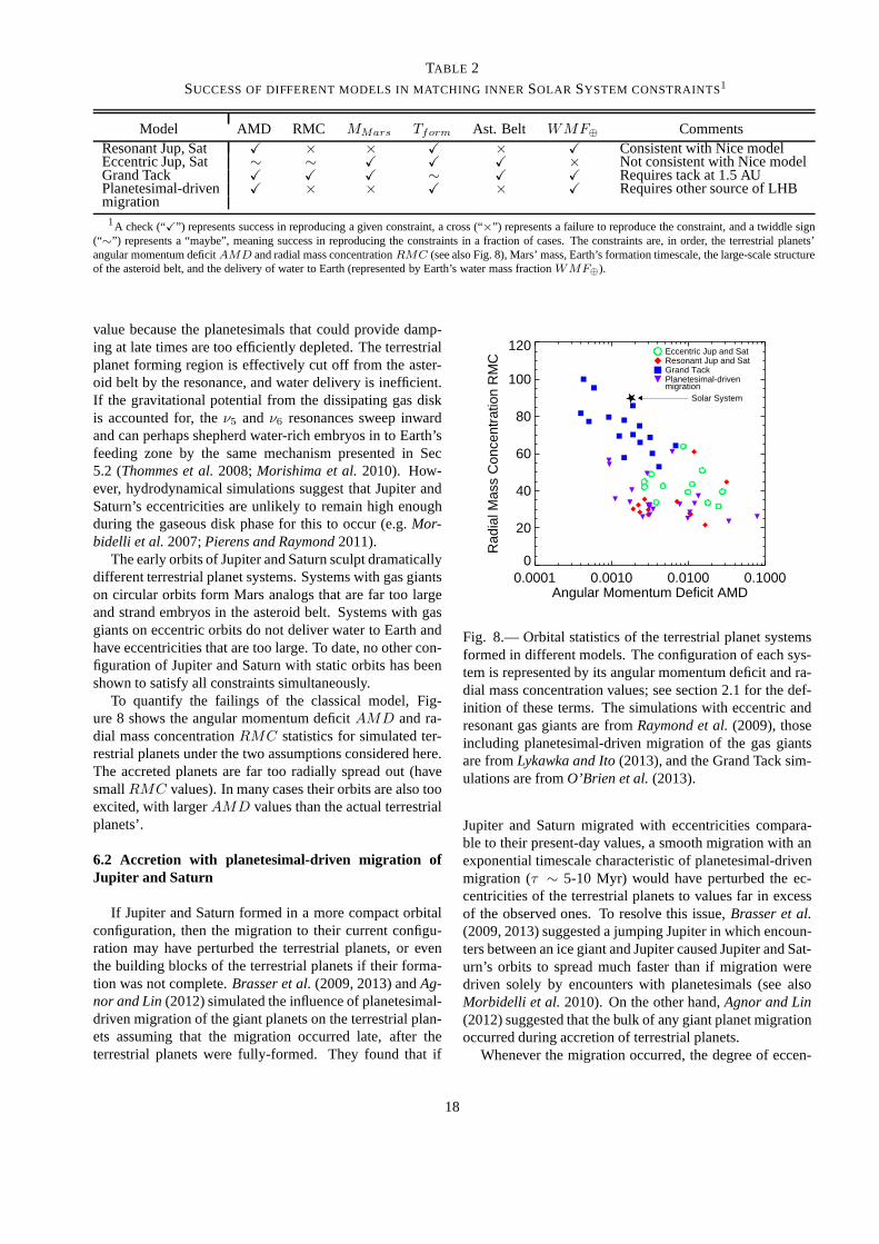
TABLE 2

SUCCESS OF DIFFERENT MODELS IN MATCHING INNERSOLAR SYSTEM CONSTRAINTS1

Model AMD RMC MMars Tform Ast. Belt WMF⊕ CommentsResonant Jup, Sat X × × X × X Consistent with Nice modelEccentric Jup, Sat ∼ ∼ X X X × Not consistent with Nice modelGrand Tack X X X ∼ X X Requires tack at 1.5 AUPlanetesimal-driven X × × X × X Requires other source of LHBmigration1A check (“X”) represents success in reproducing a given constraint, a cross (“×”) represents a failure to reproduce the constraint, and a twiddle sign

(“∼”) represents a “maybe”, meaning success in reproducing theconstraints in a fraction of cases. The constraints are, in order, the terrestrial planets’angular momentum deficitAMD and radial mass concentrationRMC (see also Fig. 8), Mars’ mass, Earth’s formation timescale,the large-scale structureof the asteroid belt, and the delivery of water to Earth (represented by Earth’s water mass fractionWMF⊕).

value because the planetesimals that could provide damp-ing at late times are too efficiently depleted. The terrestrialplanet forming region is effectively cut off from the aster-oid belt by the resonance, and water delivery is inefficient.If the gravitational potential from the dissipating gas diskis accounted for, theν5 andν6 resonances sweep inwardand can perhaps shepherd water-rich embryos in to Earth’sfeeding zone by the same mechanism presented in Sec5.2 (Thommes et al.2008;Morishima et al.2010). How-ever, hydrodynamical simulations suggest that Jupiter andSaturn’s eccentricities are unlikely to remain high enoughduring the gaseous disk phase for this to occur (e.g.Mor-bidelli et al.2007;Pierens and Raymond2011).

The early orbits of Jupiter and Saturn sculpt dramaticallydifferent terrestrial planet systems. Systems with gas giantson circular orbits form Mars analogs that are far too largeand strand embryos in the asteroid belt. Systems with gasgiants on eccentric orbits do not deliver water to Earth andhave eccentricities that are too large. To date, no other con-figuration of Jupiter and Saturn with static orbits has beenshown to satisfy all constraints simultaneously.

To quantify the failings of the classical model, Fig-ure 8 shows the angular momentum deficitAMD and ra-dial mass concentrationRMC statistics for simulated ter-restrial planets under the two assumptions considered here.The accreted planets are far too radially spread out (havesmallRMC values). In many cases their orbits are also tooexcited, with largerAMD values than the actual terrestrialplanets’.

6.2 Accretion with planetesimal-driven migration ofJupiter and Saturn

If Jupiter and Saturn formed in a more compact orbitalconfiguration, then the migration to their current configu-ration may have perturbed the terrestrial planets, or eventhe building blocks of the terrestrial planets if their forma-tion was not complete.Brasser et al.(2009, 2013) andAg-nor and Lin(2012) simulated the influence of planetesimal-driven migration of the giant planets on the terrestrial plan-ets assuming that the migration occurred late, after theterrestrial planets were fully-formed. They found that if

0.0001 0.0010 0.0100 0.1000Angular Momentum Deficit AMD

0

20

40

60

80

100

120

Rad

ial M

ass

Con

cent

ratio

n R

MC

Eccentric Jup and SatResonant Jup and SatGrand TackPlanetesimal-drivenmigration

Solar System

Fig. 8.— Orbital statistics of the terrestrial planet systemsformed in different models. The configuration of each sys-tem is represented by its angular momentum deficit and ra-dial mass concentration values; see section 2.1 for the def-inition of these terms. The simulations with eccentric andresonant gas giants are fromRaymond et al.(2009), thoseincluding planetesimal-driven migration of the gas giantsare fromLykawka and Ito(2013), and the Grand Tack sim-ulations are fromO’Brien et al.(2013).

Jupiter and Saturn migrated with eccentricities compara-ble to their present-day values, a smooth migration with anexponential timescale characteristic of planetesimal-drivenmigration (τ ∼ 5-10 Myr) would have perturbed the ec-centricities of the terrestrial planets to values far in excessof the observed ones. To resolve this issue,Brasser et al.(2009, 2013) suggested a jumping Jupiter in which encoun-ters between an ice giant and Jupiter caused Jupiter and Sat-urn’s orbits to spread much faster than if migration weredriven solely by encounters with planetesimals (see alsoMorbidelli et al.2010). On the other hand,Agnor and Lin(2012) suggested that the bulk of any giant planet migrationoccurred during accretion of terrestrial planets.

Whenever the migration occurred, the degree of eccen-

18

tricity excitation of Jupiter and Saturn is constrained by thedynamics of resonance crossing. Jupiter and Saturn arenaturally excited toegiants ∼ 0.05 but cannot reach thehigher eccentricities invoked by the eccentric Jupiter andSaturn model described above (Tsiganis et al.2005). Giventhat the eccentricity excitation is the key difference betweenthis model and those with stationary giant planets discussedabove, the only free parameter is the timing of the eccen-tricity excitation.

Two recent papers simulated the effect of planetesimal-driven migration of Jupiter and Saturn’s orbits on terrestrialplanet formation (Walsh and Morbidelli2011;Lykawka andIto 2013). In both studies terrestrial planets accrete from adisk of material which stretches from∼0.5 AU to 4.0 AU.In Walsh and Morbidelli(2011), Jupiter and Saturn are ini-tially at 5.4 and 8.7 AU respectively (slightly outside the2:1 mean motion resonance), with eccentricities compara-ble to the current ones, and migrate to 5.2 and 9.4 AU withan e-folding time of 5 Myr. In their simulations Mars istypically far too massive and the distribution of survivingplanetesimals in the asteroid belt is inconsistent with theobserved distribution.Lykawka and Ito(2013) performedsimilar simulations but included the 2:1 resonance cross-ing of Jupiter and Saturn, which provides a sharp increasein the giant planets’ eccentricities and thus in the pertur-bations felt by the terrestrial planets. They tested the tim-ing of the giant planets’ 2:1 resonance crossing between 1and 50 Myr. They found the expected strong excitation inthe asteroid belt once the giant planets’ eccentricities in-creased, but the perturbations were too small to produce asmall Mars. Although they produced four Mars analogs intheir simulations, they remained significantly more massivethan the real Mars, accreted on far longer timescales thanthe geochemically-constrained one, and stranded large em-bryos in the asteroid belt. TheirAMD andRMC valuesremain incompatible with the real Solar System (Fig. 8).

If another mechanism is invoked to explain the lateheavy bombardment, planetesimal-driven migration ofJupiter and Saturn is plausible. However, it does not ap-pear likely to have occurred as it is incapable of solving theMars problem.

6.3 The Grand Tack model

Prior to 2009, several studies of terrestrial accretion haddemonstrated an edge effect in terrestrial accretion. A dis-tribution of embryos with an abrupt edge naturally pro-duces a large mass gradient between the massive planetsthat formed within the disk and the smaller planets that werescattered beyond the disk’s edge (Wetherill 1978, 1991;Chambers and Wetherill1998;Agnor et al.1999;Cham-bers 2001; Kominami and Ida2004). These studies hadouter edges at 1.5-2 AU and generally considered their ini-tial conditions a deficiency imposed by limited computa-tional resources.

Hansen(2009) turned the tables by proposing that, ratherthan a deficiency, initial conditions with edges might actu-

ally represent the true initial state of the disk. Indeed,Mor-ishima et al.(2008) andHansen(2009) showed that mostobserved constraints could be reproduced by a disk of em-bryos spanning only from 0.7 to 1 AU. Earth and Venus aremassive because they formed within the annulus whereasMars and Mercury’s small masses are explained as edgeeffects, embryos that were scattered exterior and interior,respectively, to the annulus at early times, stranding andstarving them. Mars analogs consistently accrete on theshort observed timescale. The main unanswered questionin these studies was the origin of the edges of the annulus.

Fig. 9.—Evolution of the Grand Tack model (Walsh et al.2011).The large black dots represent the four giant planets, with sizesthat correspond to their approximate masses. Red symbols indi-cate S-class bodies and blue ones C-class bodies. There exist twocategories of C-class objects that originate between and beyondthe giant planets’ orbits. Open circles indicate planetaryembryos.The evolution of the particles includes drag forces imparted by anevolving gaseous disk.

Walsh et al.(2011) presented a mechanism to producethe outer edge of the disk by invoking migration of the gi-ant planets to dramatically sculpt the distribution of solidmaterial in the inner Solar System. Given that gas gi-ant planets must form in the presence of gaseous disksand that these disks invariably drive radial migration (Ward1997), it is natural to presume that Jupiter and Saturn musthave migrated to some extent. A Jupiter-mass planet nat-urally carves an annular gap in the gaseous disk and mi-grates inward on the local viscous timescale (Lin and Pa-paloizou1986). In contrast, a Saturn-mass planet migratesmuch more quickly because of a strong gravitational feed-back during disk clearing (Masset and Papaloizou2003).Assuming that Jupiter underwent rapid gas accretion be-fore Saturn, hydrodynamical simulations show that Jupiterwould have migrated inward relatively slowly. When Saturnunderwent rapid gas accreted it migrated inward quickly,

19

caught up to Jupiter and became trapped in 2:3 resonance.At this point the direction of migration was reversed andJupiter “tacked”, that is it changed its direction of migra-tion (Masset and Snellgrove2001;Morbidelli et al. 2007;Pierens and Nelson2008; Pierens and Raymond2011;D’Angelo and Marzari2012). The outward migration ofthe two gas giants slowed as the gaseous disk dissipated,stranding Jupiter and Saturn on resonant orbits. This nat-urally produces the initial conditions for a recently revisedversion of the Nice model (Morbidelli et al.2007;Levisonet al.2011), with Jupiter at 5.4 AU and Saturn at 7.2 AU.

This model is called theGrand Tack. One cannot knowthe precise migration history of the gas giantsa priorigiven uncertainties in disk properties and evolution.Walshet al. (2011) anchored Jupiter’s migration reversal point at1.5 AU because this truncates the inner disk of embryos andplanetesimals at 1.0 AU, creating an outer edge at the samelocation as invoked byHansen(2009). Jupiter’s formationzone was assumed to be∼ 3 − 5 AU (although a range ofvalues was tested byWalsh et al.2011), in the vicinity ofthe snow line (e.g.Sasselov and Lecar2000;Kornet et al.2004;Martin and Livio 2012), presumably a favorable lo-cation for giant planet formation. The Grand Tack modelalso proposes that the compositional gradient seen in theasteroid belt can be explained by the planetesimals’ forma-tion zones. Volatile-poor bodies (“S-class”) are primarilylocated in the inner belt and volatile-rich bodies (“C-class”)primarily in the outer belt (Gradie and Tedesco1982;De-Meo and Carry2013). The Grand Tack scenario presumesthat S-class bodies formed interior to Jupiter’s initial orbitand that C-class bodies formed exterior.

The evolution of the Grand Tack is illustrated in Fig-ure 9 (Walsh et al.2011). Jupiter and Saturn’s inwardmigration scattered S-class planetesimals from the innerdisk, with∼10% ending on eccentric orbits beyond the gi-ant planets. Meanwhile a large fraction of planetesimalsand embryos were shepherded inward by the same mecha-nism discussed in§5.2 onto orbits inside 1 AU. FollowingJupiter’s “tack” the outward-migrating gas giants first en-countered the scattered S-class planetesimals, about 1% ofwhich were scattered inward onto stable orbits in the as-teroid belt. The giant planets then encountered the disk ofC-class planetesimals that originated beyond Jupiter’s orbit.Again, a small fraction (∼ 1%) were scattered inward andtrapped in the asteroid belt. The final position of a scatteredbody depends on the orbital radius of the scattering body,in this case Jupiter. Jupiter was closer in when it scatteredthe S-class planetesimals and farther out when it scatteredthe C-class planetesimals. The S-class bodies were there-fore preferentially implanted in the inner part of the asteroidbelt and the C-class bodies preferentially in the outer partof the belt, as in the present-day belt (Gradie and Tedesco1982;DeMeo and Carry2013). The total mass of the as-teroid population is set by the need to have∼ 2 M⊕ of ma-terial remaining in the inner truncated disk of embryos andplanetesimals (to form the planets). This requirement forthe planets sets the total mass in S-class bodies implanted

into the asteroid belt as they originate from the same innerdisk. The current ratio of S-class to C-class asteroids setsthe mass in outer disk planetesimals.

The Grand Tack model reproduces many aspects of theterrestrial planets. Planets that accrete from a truncateddisk have similar properties to those inHansen(2009)andMorishima et al.(2008). Earth/Mars mass ratios areclose matches to the actual planets, and Mars’ accretiontimescale is a good match to Hf/W constraints. Figure 8shows that the angular momentum deficitAMD is sys-tematically lower than in simulations of the classical model(§6.1) and the radial mass concentrationRMC is system-atically higher (Walsh et al.2011;O’Brien et al.2013). Incontrast with other models, the Grand Tack simulations pro-vide a reasonable match to the inner Solar System.

The Grand Tack delivers water-rich material to the ter-restrial planets by a novel mechanism. As Jupiter and Sat-urn migrate outward, they scatter about 1% of the C-classasteroids that they encountered onto stable orbits in the as-teroid belt. And for every implanted C-type asteroid, 10-20C-class bodies are scattered ontounstableorbits that crossthe orbits of the terrestrial planets. These scattered C-classplanetesimals accrete with the growing terrestrial planetsand naturally deliver water. The amount of water-rich ma-terial accreted by Earth is less than in classical simulationswith stationary giant planets like the one presented in Fig.4,but is still significantly larger than the Earth’s current waterbudget (O’Brien et al.2013). The chemical signature of thedelivered water is the same as C-type asteroids (and there-fore carbonaceous chondrites), and thus provides a matchto the signature of Earth’s water (Marty and Yokochi2006).Thus, in the Grand Tack model Earth was delivered waternot by C-type asteroids but by the same parent populationas for C-type asteroids.

There remain some issues with the Grand Tack model.The accretion timescales are much faster for all of theplanets than what was typically found in previous models.This is a consequence of the removal of embryos beyond1 AU, where growth timescales are long. In simulationsMars analogs typically form in less than 10 Myr (O’Brienet al. 2013). Earth analogs form in 10-20 Myr, with giantembryo-embryo impacts occurring after 20 Myr in only amodest fraction (∼ 20%) of simulations. This is roughlya factor of two faster than the Hf-W constraints (Touboulet al. 2007;Kleine et al.2009;Konig et al.2011). How-ever, new simulations show that the accretion timescale ofthe terrestrial planets can be lengthened to match observa-tions simply by increasing the total embryo-to-planetesimalmass ratio in the annulus, which is itself an unconstrainedparameter (Jacobson et al.2013).

An open question related to the origin of Mercury’ssmall mass is the origin of theinneredge of the annulus pro-posed byHansen(2009). One possibility is that, as embryosgrow larger from the inside-out, they also become subjectto type 1 migration from the inside-out (McNeil et al.2005;Daisaka et al.2006;Ida and Lin2008). For embryo-massobjects migration is directed inward (Paardekooper et al.

20

2010), so as each embryo forms it migrates inward. If, bysome process, inward-migrating planets are removed fromthe system (presumably by colliding with the star), then aninner edge in the distribution ofsurvivingembryos couldcorrespond to the outermost orbital radius at which an em-bryo formed and was destroyed. Another possibility is thatplanetesimals could only form in a narrow annulus. If apressure bump (Johansen et al.2009) were located in thatregion it could act to concentrate small particles (Haghigh-ipour and Boss2003;Youdin and Chiang2004) and effi-ciently form planetesimals (see chapter by Johansen et al.).

7. DISCUSSION

7.1 Terrestrial planets vs. giant embryos

We think that Earth formed via successive collisions be-tween planetesimals and planetary embryos, including aprotracted stage of giant impacts between embryos. Butdoes the formation of most terrestrial planets follow thesame blueprint as Earth?

The alternative is that terrestrial exoplanets are essen-tially giant planetary embryos. They form from planetesi-mals or pebbles and do not undergo a phase of giant impactsafter the dissipation of the gaseous disk. This is a whollyreasonable possibility. Imagine a disk that only forms plan-etesimals in a few preferred locations, perhaps at pressurebumps. The planetesimals in each location could be ef-ficiently swept up into a single large embryo, perhaps bythe largest planetesimal undergoing a rapid burst of super-runaway pebble accretion. Isolated giant embryos wouldevolve with no direct contact with other embryos. Onlyif several embryos formed and migrated toward a commonlocation would embryo-embryo interactions become impor-tant, and collisions would only occur if a critical number ofembryos was present (the critical number is about 5;Mor-bidelli et al.2008;Pierens et al.2013).

Terrestrial planets and giant embryos should differ interms of their accretion timescales, their atmospheres, andperhaps their geological evolution. The timescale for thecompletion of Earth’s accretion is at least ten times longerthan the typical gas disk lifetime (see§2). Giant embryosmust form within the lifetime of the gaseous disk, whilethe mechanisms to efficiently concentrate are active. Howwould Earth be different if it had accreted ten times faster?The additional heat of formation and from trapped short-lived radionuclides could act to rapidly devolatilize the gi-ant embryo’s interior. However, giant embryos may be ableto gravitationally capture thick envelopes of gas from thedisk, at least at cooler locations within the disk (Ikoma andHori 2012). The fate of giant embryos’ volatiles remain un-studied. Nonetheless, given that only a very small amountof H and He are needed to significantly inflate a planet’s ra-dius (Fortney et al.2007), giant embryos would likely havelow bulk densities. Many low-density planets have indeedbeen discovered (Marcy et al.2013;Weiss et al.2013), al-

though we stress that this does not indicate that these aregiant embryos.

How could we tell observationally whether late phases ofgiant impacts are common? Perhaps the simplest approachwould be to search for signatures of such impacts aroundstars that no longer harbor gaseous disks. The evolutionof warm dust, detected as excess emission at mid-infraredwavelengths, has recently been measured to decline on 100Myr timescales (Meyer et al.2008;Carpenter et al.2009;Melis et al.2010). This dust is thought to trace the ter-restrial planet-forming region (Kenyon and Bromley2004)and indicates the presence of planetesimals or other largedust-producing bodies in that region. In some cases the sig-nature of specific minerals in the dust can indicate that itoriginated in a larger body. In fact, the signature of a giantimpact was reported byLisse et al.(2009) around the∼12Myr-old A star HD 172555. Given the 1-10 Myr interval be-tween giant impacts in accretion simulations and the shortlifetime of dust produced (Kenyon and Bromley2005;Meliset al. 2012), a direct measure of the frequency of systemsin which giant impacts occur will require a large sampleof young stars surveyed at mid-infrared wavelengths (e.g.,Kennedy and Wyatt2012).

7.2 Limitations of the simulations

Despite marked advances in the last few years, simula-tions of terrestrial planet formation remain both computa-tionally and physically limited. Even the best numericalintegrators (Chambers1999; Duncan et al.1998; Stadel2001) can follow the orbits of at most a few thousand par-ticles at∼ 1 AU for the>100 Myr timescales of terrestrialplanet formation. There are 3-4 orders of magnitude in un-certainty in the sizes of initial planetesimals, and a corre-sponding 9-12 orders of magnitude uncertainty in the initialnumber of planetesimals. It is clear that current simulationscannot fully simulate the conditions of planet formation ex-cept in very constrained settings (e.g.Barnes et al.2009).Simulations thus resort to including planetesimals that arefar more massive than they should be.

There exist several processes thought to be importantin planet formation that have yet to be adequately mod-eled. For example, the full evolution of a planetesimalswarm including growth, dynamical excitation, and colli-sional grinding has yet to be fully simulated (but seeBrom-ley and Kenyon2011;Levison et al.2012). In addition to thenumerical and computational challenges, this task is com-plicated by the fact that the initial distribution and sizesofplanetesimals, pebbles and dust remain at best modestly-constrained by models and observations (see chapters byJohansen et al. and Testi et al). Likewise, the masses, struc-ture and evolution of the dominant, gaseous components ofprotoplanetary disks is an issue of ongoing study.

8. SUMMARY

This chapter has flown over a broad swath of the land-scape of terrestrial planet formation. We now summarize

21

the take home messages.1. The term “terrestrial planet” is well-defined in the

confines of our Solar System but not in extra-solar planetarysystems (§1).

2. There exist ample observed and measured constraintson terrestrial planet formation models in the Solar Systemand in extra-solar planetary systems (§2).

3. There exist two models for the growth of planetaryembryos (§3). Oligarchic growth proposes that embryosgrow from swarms of planetesimals. Pebble accretion pro-poses that they grow directly from cm-sized pebbles.

4. Starting from systems of embryos and planetesimals,the main factors determining the outcome of terrestrial ac-cretion have been determined by simulations (§4). The mostimportant one is the level of eccentricity excitation of theembryo swarm – by both gravitational self-stirring and per-turbations from giant planets – as this determines the num-ber, masses and feeding zones of terrestrial planets.

5. The observed systems of hot Super Earths probablyformed by either in-situ accretion from massive disks or in-ward migration of embryos driven by interactions with thegaseous disk (§5.1). The key debate in differentiating be-tween the models is whether rocky planets that accrete insitu could retain thick gaseous envelopes.

6. The dynamical histories of giant exoplanets arethought to include gas-driven migration and planet-planetscattering. An inward-migrating gas giant forms low-massplanets interior to strong resonances and stimulates the for-mation of outer volatile-rich planets. Dynamical instabil-ities among giant planets can destroy terrestrial planets ortheir building blocks, and this naturally produces a correla-tion between debris disks and terrestrial planets (§5.2).

7. Historical simulations of terrestrial planet formationcould not reproduce Mars’ small mass (§6.1). This is calledthesmall Mars problem. Simulations can reproduce Mars’small mass by invoking large initial eccentricities of Jupiterand Saturn at their current orbital radii. Invoking earlyplanetesimal-driven migration of Jupiter and Saturn doesnot produce a small Mars (§6.2).

8. TheGrand Tackmodel proposes that Jupiter migratedinward to 1.5 AU then back outward due to disk torques be-fore and after Saturn’s formation (§6.3). The inner disk wastruncated at 1 AU, producing a large Earth/Mars mass ratio.Water was delivered to the terrestrial planets in the form ofC-class bodies scattered inward during the gas giants’ out-ward migration.

Finally, it remains unclear whether most systems of ter-restrial planets undergo phases of giant collisions betweenembryos during their formation (§7.1).

Acknowledgments. We are grateful to a long list of col-leagues whose work contributed to this chapter. S.N.R.thanks NASA’s Astrobiology Institute for their funding viathe University of Washington, University of Colorado, andVirtual Planetary Laboratory lead teams. S.N.R. and A.M.thank the CNRS’s Programme Nationale de Planetologie.KJW acknowledges support from NLSI CLOE.

REFERENCES

Adachi I. et al. (1976)Progress of Theoretical Physics, 56, 1756.Adams E. R. et al. (2008)Astrophys. J., 673, 1160.Adams F. C. and Laughlin G. (2003)Icarus, 163, 290.Agnor C. and Asphaug E. (2004)Astrophys. J. Lett., 613, L157.Agnor C. B. and Lin D. N. C. (2012)Astrophys. J., 745, 143.Agnor C. B. et al. (1999)Icarus, 142, 219.Alexander S. G. and Agnor C. B. (1998)Icarus, 132, 113.Andrews S. M. and Williams J. P. (2007a)Astrophys. J., 671, 1800.Andrews S. M. and Williams J. P. (2007b)Astrophys. J., 659, 705.Armitage P. J. (2007)Astrophys. J., 665, 1381.Asphaug E. (2010)Chemie der Erde / Geochemistry, 70, 199.Asphaug E. et al. (2006)Nature, 439, 155.Baraffe I. et al. (2004)Astron. Astrophys., 419, L13.Baraffe I. et al. (2006)Astron. Astrophys., 450, 1221.Barnes R. et al. (2009)Icarus, 203, 626.Batalha N. M. et al. (2013)Astrophys. J. Suppl., 204, 24.Batygin K. and Morbidelli A. (2013)Astron. J., 145, 1.Beauge C. and Nesvorny D. (2012)Astrophys. J., 751, 119.Benz W. et al. (2007)Space Sci. Rev., 132, 189.Bond J. C. et al. (2010)Icarus, 205, 321.Bonfils X. et al. (2013)Astron. Astrophys., 549, A109.Bottke W. F. et al. (2010)Science, 330, 1527.Brasser R. et al. (2009)Astron. Astrophys., 507, 1053.Brasser R. et al. (2013)Mon. Not. R. Astron. Soc..Bromley B. C. and Kenyon S. J. (2011)Astrophys. J., 731, 101.Buchhave L. A. et al. (2012)Nature, 486, 375.Canup R. M. (2012)Science, 338, 1052.Carpenter J. M. et al. (2009)Astrophys. J. Suppl., 181, 197.Carter-Bond J. C. et al. (2012)Astrophys. J., 760, 44.Chambers J. (2006)Icarus, 180, 496.Chambers J. (2008)Icarus, 198, 256.Chambers J. E. (1999)Mon. Not. R. Astron. Soc., 304, 793.Chambers J. E. (2001)Icarus, 152, 205.Chambers J. E. (2010)Icarus, 208, 505.Chambers J. E. (2013)Icarus, 224, 43.Chambers J. E. and Cassen P. (2002)Meteoritics and Planetary

Science, 37, 1523.Chambers J. E. and Wetherill G. W. (1998)Icarus, 136, 304.Chambers J. E. et al. (1996)Icarus, 119, 261.Chapman C. R. et al. (2007)Icarus, 189, 233.Chatterjee S. et al. (2008)Astrophys. J., 686, 580.Chiang E. and Laughlin G. (2013)Mon. Not. R. Astron. Soc., 431,

3444.Cohen B. A. et al. (2000)Science, 290, 1754.Correia A. C. M. and Laskar J. (2009)Icarus, 201, 1.Cossou C. et al. (2013)arXiv:1307.2897.Cresswell P. and Nelson R. P. (2008)Astron. Astrophys., 482, 677.Cresswell P. et al. (2007)Astron. Astrophys., 473, 329.Cuk M. and Stewart S. T. (2012)Science, 338, 1047.Cumming A. et al. (2008)PASP, 120, 531.Daisaka J. K. et al. (2006)Icarus, 185, 492.D’Angelo G. and Marzari F. (2012)Astrophys. J., 757, 50.Dauphas N. and Pourmand A. (2011)Nature, 473, 489.Davis S. S. (2005)Astrophys. J. Lett., 627, L153.Day J. M. D. et al. (2007)Science, 315, 217.DeMeo F. E. and Carry B. (2013)Icarus, 226, 723.Desch S. J. (2007)Astrophys. J., 671, 878.Dones L. and Tremaine S. (1993)Icarus, 103, 67.Drake M. J. and Righter K. (2002)Nature, 416, 39.Duncan M. J. et al. (1998)Astron. J., 116, 2067.

22

Eisner J. A. (2012)Astrophys. J., 755, 23.Eisner J. A. et al. (2008)Astrophys. J., 683, 304.Elser S. et al. (2012)Icarus, 221, 859.Erkaev N. V. et al. (2007)Astron. Astrophys., 472, 329.Fabrycky D. and Tremaine S. (2007)Astrophys. J., 669, 1298.Fang J. and Margot J.-L. (2013)Astrophys. J., 767, 115.Fedele D. et al. (2010)Astron. Astrophys., 510, A72.Fernandez J. A. and Ip W. (1984)Icarus, 58, 109.Fischer D. A. and Valenti J. (2005)Astrophys. J., 622, 1102.Fogg M. J. and Nelson R. P. (2005)Astron. Astrophys., 441, 791.Fogg M. J. and Nelson R. P. (2007)Astron. Astrophys., 461, 1195.Fogg M. J. and Nelson R. P. (2009)Astron. Astrophys., 498, 575.Ford E. B. and Rasio F. A. (2006)Astrophys. J. Lett., 638, L45.Fortney J. J. et al. (2007)Astrophys. J., 659, 1661.Fressin F. et al. (2013)Astrophys. J., 766, 81.Gaidos E. et al. (2007)Science, 318, 210.Geiss J. and Gloeckler G. (1998)Space Sci. Rev., 84, 239.Genda H. and Abe Y. (2005)Nature, 433, 842.Genda H. et al. (2012)Astrophys. J., 744, 137.Ghezzi L. et al. (2010)Astrophys. J., 720, 1290.Gladman B. J. et al. (1997)Science, 277, 197.Goldreich P. and Tremaine S. (1980)Astrophys. J., 241, 425.Goldreich P. et al. (2004)Astrophys. J., 614, 497.Gonzalez G. (1997)Mon. Not. R. Astron. Soc., 285, 403.Gould A. et al. (2010)Astrophys. J., 720, 1073.Gradie J. and Tedesco E. (1982)Science, 216, 1405.Greaves J. S. et al. (2006)Mon. Not. R. Astron. Soc., 366, 283.Greenberg R. et al. (1978)Icarus, 35, 1.Grimm R. E. and McSween H. Y. (1993)Science, 259, 653.Haghighipour N. and Boss A. P. (2003)Astrophys. J., 583, 996.Haisch Jr. K. E. et al. (2001)Astrophys. J. Lett., 553, L153.Hansen B. M. S. (2009)Astrophys. J., 703, 1131.Hansen B. M. S. and Murray N. (2012)Astrophys. J., 751, 158.Hansen B. M. S. and Murray N. (2013)Astrophys. J., 775, 53.Hartogh P. et al. (2011)Nature, 478, 218.Hayashi C. et al. (1985) in:Protostars and Planets II, (edited by

D. C. Black and M. S. Matthews), pp. 1100–1153.Hillenbrand L. A. et al. (2008)Astrophys. J., 677, 630.Howard A. W. et al. (2010)Science, 330, 653.Howard A. W. et al. (2012)Astrophys. J. Suppl., 201, 15.Hubbard W. B. et al. (2007a)Astrophys. J. Lett., 658, L59.Hubbard W. B. et al. (2007b)Icarus, 187, 358.Ida S. and Lin D. N. C. (2008)Astrophys. J., 673, 487.Ida S. and Makino J. (1992)Icarus, 96, 107.Ida S. and Makino J. (1993)Icarus, 106, 210.Ida S. et al. (2008)Astrophys. J., 686, 1292.Ikoma M. and Hori Y. (2012)Astrophys. J., 753, 66.Jackson B. et al. (2010)Mon. Not. R. Astron. Soc., 407, 910.Jacobson S. et al. (2013) in:Protostars and Planets VI, Heidel-

berg, July 15-20, 2013. Poster #2H024, p. 24.Jin L. et al. (2008)Astrophys. J. Lett., 674, L105.Johansen A. and Lacerda P. (2010)Mon. Not. R. Astron. Soc., 404,

475.Johansen A. et al. (2006)Astrophys. J., 636, 1121.Johansen A. et al. (2007)Nature, 448, 1022.Johansen A. et al. (2009)Astrophys. J., 697, 1269.Juric M. and Tremaine S. (2008)Astrophys. J., 686, 603.Kaib N. A. et al. (2013)Nature, 493, 381.Kennedy G. M. and Wyatt M. C. (2012)Mon. Not. R. Astron. Soc.,

426, 91.Kenyon S. J. and Bromley B. C. (2004)Astrophys. J. Lett., 602,

L133.

Kenyon S. J. and Bromley B. C. (2005)Astron. J., 130, 269.Kenyon S. J. and Bromley B. C. (2006)Astron. J., 131, 1837.Kimura K. et al. (1974)Geochim. Cosmochim. Acta, 38, 683.Kleine T. et al. (2002)Nature, 418, 952.Kleine T. et al. (2009)Geochim. Cosmochim. Acta, 73, 5150.Kobayashi H. and Dauphas N. (2013)Icarus, 225, 122.Kobayashi H. and Tanaka H. (2010a)Icarus, 206, 735.Kobayashi H. and Tanaka H. (2010b)Icarus, 206, 735.Kokubo E. and Genda H. (2010)Astrophys. J. Lett., 714, L21.Kokubo E. and Ida S. (1995)Icarus, 114, 247.Kokubo E. and Ida S. (1996)Icarus, 123, 180.Kokubo E. and Ida S. (1998)Icarus, 131, 171.Kokubo E. and Ida S. (2000)Icarus, 143, 15.Kokubo E. and Ida S. (2002)Astrophys. J., 581, 666.Kokubo E. and Ida S. (2007)Astrophys. J., 671, 2082.Kokubo E. et al. (2006)Astrophys. J., 642, 1131.Kominami J. and Ida S. (2004)Icarus, 167, 231.Konig S. et al. (2011)Geochim. Cosmochim. Acta, 75, 2119.Kornet K. et al. (2004)Astron. Astrophys., 417, 151.Kretke K. A. and Lin D. N. C. (2012)Astrophys. J., 755, 74.Krivov A. V. (2010) Research in Astronomy and Astrophysics, 10,

383.Lambrechts M. and Johansen A. (2012)Astron. Astrophys., 544,

A32.Lammer H. et al. (2003)Astrophys. J. Lett., 598, L121.Laskar J. (1997)Astron. Astrophys., 317, L75.Laws C. et al. (2003)Astron. J., 125, 2664.Lecuyer C. et al. (1998)Chem. Geol., 145, 249.Leger A. et al. (2009)Astron. Astrophys., 506, 287.Leinhardt Z. M. and Stewart S. T. (2012)Astrophys. J., 745, 79.Levison H. F. and Agnor C. (2003)Astron. J., 125, 2692.Levison H. F. et al. (2011)Astron. J., 142, 152.Levison H. F. et al. (2012)Astron. J., 144, 119.Lin D. N. C. and Papaloizou J. (1986)Astrophys. J., 309, 846.Lin D. N. C. et al. (1996)Nature, 380, 606.Lissauer J. J. (1987)Icarus, 69, 249.Lissauer J. J. and Kary D. M. (1991)Icarus, 94, 126.Lissauer J. J. and Stevenson D. J. (2007)Protostars and Planets

V, pp. 591–606.Lissauer J. J. et al. (2011)Nature, 470, 53.Lisse C. M. et al. (2008)Astrophys. J., 673, 1106.Lisse C. M. et al. (2009)Astrophys. J., 701, 2019.Lodders K. (2003)Astrophys. J., 591, 1220.Lommen D. et al. (2007)Astron. Astrophys., 462, 211.Looney L. W. et al. (2003)Astrophys. J., 592, 255.Lopez E. and Fortney J. (2013)ArXiv e-prints.Lovis C. et al. (2011)Astron. Astrophys., 528, A112.Lykawka P. S. and Ito T. (2013)Astrophys. J., 773, 65.Makino J. et al. (1998)New A, 3, 411.Mandell A. M. et al. (2007)Astrophys. J., 660, 823.Mann A. W. et al. (2012)Astrophys. J., 753, 90.Marcy G. W. et al. (2013)Submitted.Martin R. G. and Livio M. (2012)Mon. Not. R. Astron. Soc., 425,

L6.Marty B. (2012)Earth and Planetary Science Letters, 313, 56.Marty B. and Yokochi R. (2006)Rev. Mineral Geophys., 62, 421.Marzari F. and Weidenschilling S. J. (2002)Icarus, 156, 570.Masset F. and Snellgrove M. (2001)Mon. Not. R. Astron. Soc.,

320, L55.Masset F. S. and Casoli J. (2010)Astrophys. J., 723, 1393.Masset F. S. and Papaloizou J. C. B. (2003)Astrophys. J., 588,

494.

23

Masset F. S. et al. (2006)Astrophys. J., 642, 478.Matsumura S. et al. (2010)Astrophys. J., 714, 194.Mayor M. et al. (2009)Astron. Astrophys., 507, 487.Mayor M. et al. (2011)arXiv:1109.2497.McNeil D. et al. (2005)Astron. J., 130, 2884.Melis C. et al. (2010)Astrophys. J. Lett., 717, L57.Melis C. et al. (2012)Nature, 487, 74.Meyer M. R. et al. (2008)Astrophys. J. Lett., 673, L181.Moeckel N. and Armitage P. J. (2012)Mon. Not. R. Astron. Soc.,

419, 366.Moeckel N. et al. (2008)Astrophys. J., 688, 1361.Moorhead A. V. and Adams F. C. (2005)Icarus, 178, 517.Morbidelli A. et al. (2000)Meteoritics and Planetary Science, 35,

1309.Morbidelli A. et al. (2007)Astron. J., 134, 1790.Morbidelli A. et al. (2008)Astron. Astrophys., 478, 929.Morbidelli A. et al. (2010)Astron. J., 140, 1391.Morbidelli A. et al. (2012)Annual Review of Earth and Planetary

Sciences, 40, 251.Morishima R. et al. (2008)Astrophys. J., 685, 1247.Morishima R. et al. (2010)Icarus, 207, 517.Morishima R. et al. (2013)Earth and Planetary Science Letters,

366, 6.Moro-Martın A. et al. (2007)Astrophys. J., 658, 1312.Mundy L. G. et al. (2000)Protostars and Planets IV, pp. 355–+.Murray N. et al. (1998)Science, 279, 69.Murray-Clay R. et al. (2011) in:Extreme Solar Systems, p. 804.Murray-Clay R. A. et al. (2009)Astrophys. J., 693, 23.Nagasawa M. et al. (2008)Astrophys. J., 678, 498.Naoz S. et al. (2011)Nature, 473, 187.Nimmo F. and Agnor C. B. (2006)Earth and Planetary Science

Letters, 243, 26.Nimmo F. and Kleine T. (2007)Icarus, 191, 497.O’Brien D. P. et al. (2006)Icarus, 184, 39.O’Brien D. P. et al. (2013)Submitted.Ogihara M. and Ida S. (2009)Astrophys. J., 699, 824.Ormel C. W. and Klahr H. H. (2010)Astron. Astrophys., 520, A43.Ormel C. W. et al. (2010)Astrophys. J. Lett., 714, L103.Paardekooper S.-J. et al. (2010)Mon. Not. R. Astron. Soc., 401,

1950.Pascucci I. et al. (2009)Astrophys. J., 696, 143.Perez L. M. et al. (2012)Astrophys. J. Lett., 760, L17.Pierens A. and Nelson R. P. (2008)Astron. Astrophys., 482, 333.Pierens A. and Raymond S. N. (2011)Astron. Astrophys., 533,

A131.Pierens A. et al. (2013)Astron. Astrophys., 558, A105.Rafikov R. R. (2004)Astron. J., 128, 1348.Rasio F. A. and Ford E. B. (1996)Science, 274, 954.Raymond S. N. (2006)Astrophys. J. Lett., 643, L131.Raymond S. N. and Cossou C. (2014)arXiv:1401.3743.Raymond S. N. et al. (2004)Icarus, 168, 1.Raymond S. N. et al. (2005)Astrophys. J., 632, 670.Raymond S. N. et al. (2006a)Science, 313, 1413.Raymond S. N. et al. (2006b)Icarus, 183, 265.Raymond S. N. et al. (2007a)Astrophys. J., 669, 606.Raymond S. N. et al. (2007b)Astrobiology, 7, 66.Raymond S. N. et al. (2008)Mon. Not. R. Astron. Soc., 384, 663.Raymond S. N. et al. (2009)Icarus, 203, 644.Raymond S. N. et al. (2010)Astrophys. J., 711, 772.Raymond S. N. et al. (2011)Astron. Astrophys., 530, A62.Raymond S. N. et al. (2012)Astron. Astrophys., 541, A11.Raymond S. N. et al. (2013)Icarus, 226, 671.

Rodmann J. et al. (2006)Astron. Astrophys., 446, 211.Safronov V. S. (1969)Evoliutsiia doplanetnogo oblaka.Santos N. C. et al. (2001)Astron. Astrophys., 373, 1019.Sasselov D. D. and Lecar M. (2000)Astrophys. J., 528, 995.Schlichting H. E. et al. (2012)Astrophys. J., 752, 8.Scholz A. et al. (2006)Astrophys. J., 645, 1498.Stadel J. G. (2001)Cosmological N-body simulations and their

analysis, Ph.D. thesis, University of Washington.Stewart S. T. and Leinhardt Z. M. (2012)Astrophys. J., 751, 32.Sumi T. et al. (2011)Nature, 473, 349.Tanaka H. and Ward W. R. (2004)Astrophys. J., 602, 388.Tera F. et al. (1974)Earth and Planetary Science Letters, 22, 1.Terquem C. and Papaloizou J. C. B. (2007)Astrophys. J., 654,

1110.Thommes E. W. et al. (2003)Icarus, 161, 431.Thommes E. W. et al. (2008)Science, 321, 814.Touboul M. et al. (2007)Nature, 450, 1206.Tsiganis K. et al. (2005)Nature, 435, 459.Udry S. et al. (2007)Astron. Astrophys., 469, L43.Valencia D. et al. (2007)Astrophys. J., 665, 1413.Veras D. and Armitage P. J. (2004)Mon. Not. R. Astron. Soc., 347,

613.Veras D. and Armitage P. J. (2005)Astrophys. J. Lett., 620, L111.Veras D. and Armitage P. J. (2006)Astrophys. J., 645, 1509.Walker R. J. (2009)Chemie der Erde / Geochemistry, 69, 101.Walsh K. J. and Morbidelli A. (2011)Astron. Astrophys., 526,

A126.Walsh K. J. et al. (2011)Nature, 475, 206.Ward W. R. (1986)Icarus, 67, 164.Ward W. R. (1997)Icarus, 126, 261.Weidenschilling S. J. (1977)Astrophys. Space Sci., 51, 153.Weidenschilling S. J. and Marzari F. (1996)Nature, 384, 619.Weiss L. and Marcy G. W. (2013)arXiv:1312.0936.Weiss L. M. et al. (2013)Astrophys. J., 768, 14.Wetherill G. W. (1978) in:IAU Colloq. 52: Protostars and Plan-

ets, (edited by T. Gehrels), pp. 565–598.Wetherill G. W. (1985)Science, 228, 877.Wetherill G. W. (1991) in:Lunar and Planetary Institute Science

Conference Abstracts, vol. 22 of Lunar and Planetary Inst.Technical Report, p. 1495.

Wetherill G. W. (1996)Icarus, 119, 219.Wetherill G. W. and Stewart G. R. (1989)Icarus, 77, 330.Wetherill G. W. and Stewart G. R. (1993)Icarus, 106, 190.Williams J. P. and Cieza L. A. (2011)Annu. Rev. Astron. Astro-

phys., 49, 67.Wilner D. J. et al. (2005)Astrophys. J. Lett., 626, L109.Wright J. T. et al. (2008)Astrophys. J. Lett., 683, L63.Wyatt M. C. (2008)Annu. Rev. Astron. Astrophys., 46, 339.Yasui C. et al. (2009)Astrophys. J., 705, 54.Yelle R. V. (2004)Icarus, 170, 167.Yin Q. et al. (2002)Nature, 418, 949.Yoshinaga K. et al. (1999)Icarus, 139, 328.Youdin A. N. and Chiang E. I. (2004)Astrophys. J., 601, 1109.Youdin A. N. and Goodman J. (2005)Astrophys. J., 620, 459.Zhou J.-L. et al. (2005)Astrophys. J. Lett., 631, L85.

This 2-column preprint was prepared with the AAS LATEX macros v5.2.

24