The Diverse Origins of Terrestrial-Planet Systems

Makiko NagasawaNational Astronomical Observatory of Japan

Edward W. ThommesCanadian Institute for Theoretical Astrophysics

Scott J. KenyonSmithsonian Astrophysical Observatory

Benjamin C. BromleyUniversity of Utah

Douglas N. C. LinUniversity of California, Santa Cruz

We review the theory of terrestrial planet formation as it currently stands. In an-ticipation of forthcoming observational capabilities, the central theoretical issues tobe addressed are: 1) what is the frequency of terrestrial planets around nearby stars,2) what mechanisms determine the mass distribution, dynamical structure and thestability of terrestrial-planet systems, and 3) what processes regulated the chrono-logical sequence of gas and terrestrial planet formation in the Solar System? In thecontext of Solar System formation, the last stage of terrestrial planet formation willbe discussed along with cosmochemical constraints and different dynamical archi-tectures together with important processes such as runaway and oligarchic growth.Observations of dust around other stars, combined with models of dust productionduring accretion, give us a window on exo-terrestrial planet formation. We discussthe latest results from such models, including predictions which will be tested bynext-generation instruments such as GMT and ALMA.

1. INTRODUCTION

Our home in the Solar System: Third planet, 150 mil-lion km from the Sun, 70 percent ocean, possessing a largemoon and a moderate climate. How was it born, and howdid it grow? How ubiquitous are planets like it in the uni-verse? Such questions have been asked throughout humanhistory. Recent advances in both theory and observationhave brought us closer to the answers.

Following the first discovery of an extrasolar planetaround 51 Peg, more than 150 planets have been announced,including such fascinating specimens as the multi-planetsystem of Upsilon Andromeda, and the Neptune-massplanet in 55 Cnc (e.g., Mayor and Queloz, 1995; Butleret al., 1999; McArthur et al., 2004). In just ten years,observational techniques have come to within an order ofmagnitude of being able to find an Earth-mass planet. Thedetected extrasolar planets turned on their head the stan-dard models of planetary formation (e.g., Safronov, 1969;Hayashi et al., 1985) which were proposed in the 1970s.The seemingly sensible architecture of our Solar System,with four terrestrial planets orbiting inside 2AU, plus gas

and icy planets orbiting outside the “snow line”, all onreassuringly circular orbits, turned out to be far from theonly possible configuration. On the contrary, short or-bital periods, high eccentricities and large planetary masseshave made for a diversity of planetary systems unimag-ined a decade ago (Marcy et al., 2004; Mayor et al., 2004).The theory of planet formation has likewise made rapidprogress, helped by these observations and by increases incomputing power. We can now numerically simulate manyaspects of the formation process in great detail. Thus wehave moved well beyond the dawn of planetary science,into an era of fast-paced development. It is thus an excitingtime to review the current state of the theory of terrestrialplanet formation.

2. BACKGROUND

In the standard scenario, terrestrial planets form through1) dust aggregation and settling in the protoplanetary disk,2) planetesimal formation from grains in a thin midplane,3) protoplanet accretion from planetesimals, and 4) fi-nal accumulation by giant impacts. Here, we begin with

1

an overview of the first stages and then focus on chaoticgrowth, the last stage of terrestrial planetary formation.

Although analytic studies are the foundation for this pic-ture, numerical calculations are essential to derive the phys-ical properties of planetary systems. There are two broadclasses of simulations. The statistical approach (Wetherilland Stewart, 1989, 1993) can follow collisional growth –including collisional disruption and evolution of dust grains– over long times with modest computational effort (Inabaet al., 2001, and references therein). This approach worksbest for the first three stages, where statistical approxima-tions are accurate and large-scale dynamical interactions aresmall. Direct N-body calculations (Kokubo et al., 1998;Chambers, 2001) are computationally expensive but canfollow key dynamical phenomena such as resonant inter-actions important during the final stages of planet growth.All calculation benefit from advances in computing power.In particular, N-body simulations no longer require an ar-tificial scaling parameter to speed up the evolution and arethus more reliable (Kokubo and Ida 2000).

2.1. From Dust to Planetesimals

The growth of km-sized planetesimals involves complexinteractions between dust and gas within the protoplanetarydisk (e.g., Dominik et al., this volume; Weidenschilling andCuzzi, 1993; Ward, 2000). The vertical component of thestar’s gravity pulls mm-sized and larger grains toward themidplane, where they settle into a thin disk. Smaller grainsare more strongly coupled to turbulence in the gas and re-main suspended above the midplane. The gas disk is partlypressure-supported and rotates at slightly less than Keple-rian velocity. The dust grains thus feel a headwind and un-dergo orbital decay by aero-drag. The drag is strongest form-size particles (e.g., Adachi et al., 1976; Tanaka and Ida,1999), which fall into the star from 1 AU in ∼ 100 yr. Itis not yet clear whether m-sized objects have enough timeto grow directly to km-sized planetesimals which are safefrom gas drag (Dominik et al., this volume).

Dynamical instability mechanisms sidestep the difficul-ties of direct accumulation of planetesimals (e.g., Goldreichand Ward, 1973; Youdin and Shu, 2002). If the turbulencein the gas is small, the dusty midplane becomes thinner andthinner until groups of particles overcome the local Jeanscriterion – where their self-gravity overcomes tidal forcesfrom the central star – and ‘collapse’ into larger objects.Although this gravitational instability is promising, it is stilluncertain whether the turbulence in the disk is large enoughto prevent the instability (Weidenschiling and Cuzzi, 1993;Weidenschiling, 1995). The range of planetesimal sizes pro-duced by the instability is also uncertain.

2.2. From Planetesimals to Protoplanets

Once planetesimals reach km sizes, they begin to inter-act gravitationally. Collisions produce mergers and tend tocircularize the orbits. Long range gravitational interactionsexchange kinetic energy (dynamical friction) and angular

momentum (viscous stirring), redistributing orbital energyamong planetesimals. Gas drag damps the orbits of plan-etesimals. For planetesimals without an external perturber,the collisional cross-section is

σ = πd2fg = πd2

(1 +

v2esc

v2

), (1)

where d is the radius of a particle with mass m, v is itsvelocity relative to a Keplerian orbit, and v2

esc = 2Gm/d isthe escape velocity (Wetherill, 1990; Ohtsuki et al., 1993;Kortenkamp et al., 2000). With no outside perturbations,v ≈ vesc, and gravitational focusing factors, fg ∼ 1, aresmall. Thus, growth is slow and orderly (Safronov, 1969).

During orderly growth, long range gravitational inter-actions between growing planetesimals become important.Small particles damp the orbits of larger particles; largerparticles stir up the orbits of smaller particles (Wetherill andStewart, 1993; Kokubo and Ida, 1995). In cases where gasdrag is negligible compared to viscous stirring, the relativeorbital velocities of the largest (’l’) and smallest (’s’) bodiesreach an approximate steady-state with

vl

vs=

(Σl

Σs

)n

, (2)

where n ≈ 1/4 to 1/2 and Σ is the surface density (Kokuboand Ida, 1996; Goldreich et al., 2004). When planetesimalsare small, Σl/Σs 1 and vl/vs < 1. As planetesimalsgrow, their escape velocity also grows, which leads to fg 1 and the onset of runaway growth.

Runaway growth depends on a positive feedback be-tween dynamical friction and gravitational focusing. Dy-namical friction produces a velocity distribution that de-clines roughly monotonically with increasing mass (eq. 2).Although gas drag damps the orbits of these objects andkeeps their velocities less than vesc, dynamical friction andviscous stirring maintain the small velocities of the largestobjects. Because they have the largest vesc and the smallestv, the largest objects have the largest gravitational cross-sections and the largest growth rates (eq. 1). Thus, a fewlarge objects grow fastest and “run away” from the ensem-ble of planetesimals (Wetherill and Stewart, 1989, 1993;Kokubo and Ida, 1996).

Runaway growth also depends on a broad size distribu-tion. For planetesimals with masses, m1 and m2, and rela-tive velocities, v1 and v2, stirring from dynamical friction is∼ (m1v

21 − m2v

22). With v1 ≈ v2 initially, dynamical fric-

tion becomes important when m2 10m1. For planetes-imals at 1 AU, dynamical friction dominates the evolutionwhen m2 ∼ (104 − 106)m1 ∼ 1020–1024 g for planetesi-mals with radii of 1–10 km (m1 ∼ 1016–1019 g; Ohtsuki etal., 1993). The typical timescale for planetesimals to reachm2 ∼ 1024 g is ∼ 104–105 yr at 1 AU (Wetherill and Stew-art, 1989, 1993; Weidenschilling et al., 1997).

As a few protoplanets contain an ever increasing frac-tion of the total mass, two processes halt runaway growth(Ida and Makino, 1993; Kokubo and Ida, 1998). Proto-

2

planets stir up leftover planetesimals, reducing their grav-itational cross-sections. With less mass in planetesimals,dynamical friction between the smallest planetesimals andthe largest protoplanets cannot maintain the low velocitiesof the largest objects, reducing gravitational cross-sectionsfurther (eq.1, 2). Because the largest protoplanet stirs up itssurroundings the most, its growth slows down the most, al-lowing smaller protoplanets to catch up before their growthrates also slow down. This process results in an “oli-garchy” of (locally) similar-mass protoplanets (Kokubo andIda 1998). Protoplanets reach oligarchy faster closest to thecentral star, where the surface density of dust is largest andthe orbital period is shortest. Thus, the onset of oligarchysweeps from the inside to the outside of the disk. Althoughsmaller “oligarchs” grow faster than larger ones, oligarchscontinue to sweep up leftover planetesimals and thus con-tain a larger and larger fraction of the total mass in the disk.

During oligarchic growth, protoplanets isolate them-selves from their neighbors. Mutual gravitational inter-actions push them apart to maintain relative separations of∼ 10 Hill radii (rH; Kokubo and Ida, 1995, 1998). Dy-namical friction circularizes their orbits. The large orbitalseparations and circular orbits yield a maximum “isolationmass,” derived from the mass of planetesimals within the∼ 10rH annulus, ∼ 0.1–0.2 M⊕, roughly 10%–20% of anEarth mass (see below). The typical timescale to reach thisisolation mass is ∼ 105–106 yr (Kokubo and Ida, 1998).

2.3. From Protoplanets to Planets

With isolation masses a small fraction of the mass of theEarth or Venus, dynamical interactions among the oligarchsmust become more energetic to complete terrestrial planetformation. When oligarchs have accumulated most of theplanetesimals in their isolation zones, dynamical frictionbetween planetesimals and oligarchs cannot balance dy-namical interactions among the oligarchs. Oligarchy ends.Chaotic growth, where planets grow by giant impacts andcontinued accretion of small planetesimals, begins.

The transition from oligarchy to chaos depends on thebalance between damping and dynamical interactions. Withno external perturber – a massive planet or a binary com-panion – the transition occurs when the surface density inoligarchs roughly equals the surface density in planetesi-mals (Goldreich et al., 2004; Kenyon and Bromley, 2006).The transition occurs in ∼ 10 Myr (e.g., Chambers et al.,1996). Dynamical perturbations by a Jovian planet or a bi-nary companion shorten this timescale (Ito and Tanikawa,1999); damping processes lengthen it (Iwasaki et al. 2001,2002). Once isolation is overcome, protoplanets grow toplanets in ∼ 10–300 Myr (e.g., Chambers and Wetherill,1998; Chambers, 2001; Kenyon and Bromley, 2006).

2.4. Outcomes of Numerical Simulations

Attempts to simulate the assembly of terrestrial planetsusing statistical and N-body approaches began in the late1970’s (Greenberg et al., 1978). Although statistical meth-

ods have evolved from single annulus (Wetherill and Stew-art, 1993) to multiannulus techniques (Weidenschilling etal., 1997), the main result is robust: all calculations yield10–40 isolated Mars-sized protoplanets in roughly circu-lar orbits and many leftover planetesimals on highly eccen-tric orbits. During oligarchic growth, fragmentation of theleftovers introduces uncertainties in the timescales and out-comes, as described in Section 3 and Section 4.

With tens to a few hundred protoplanets remaining at theend of oligarchic growth, direct N-body simulations providethe only way to follow the orbital interactions over hundredsof Myr. Indeed, the first direct N-body (Cox and Lewis,1980; Lecar and Aarseth, 1986) and Monte-Carlo Opik-Arnold scheme simulations (e.g., Wetherill, 1985, 1996),demonstrate that collisions of Moon-sized objects yield “so-lar systems” containing at least one planet with m M⊕/3at ∼ 1 AU around a solar-mass star. However, these simu-lations also show that the outcomes are stochastic and sen-sitive to the initial number and orbit distributions of the oli-garchs. Thus, each set of initial conditions requires manyrealizations to derive statistically meaningful results.

Several groups have performed full N-body simulationsof chaotic growth with and without dynamical influencefrom Jovian planets (e.g., Chambers and Wetherill, 1998;Agnor et al., 1999; Chambers, 2001; Kominami and Ida,2002, 2004; Kokubo et al., 2006a). The simulations startwith ∼ 20–200 oligarchs in circular or modestly ellipticalorbits, with a radial surface density that declines with semi-major axis. Multiple runs (∼ 10–200) having identical ini-tial conditions except for, typically, random variations inorbital phase, provide a first measure of the repeatabilityof the results. These calculations yield similar results forthe masses, spin angular momenta, and orbital propertiesof planets and leftover oligarchs. On timescales of 100–300 Myr, most simulations yield planets with (i) masses andsemimajor axes similar to the terrestrial planets in the SolarSystem, (ii) orbital eccentricities and inclinations somewhatlarger than those in the Solar System, and (iii) spins dom-inated by the last few giant impacts. Thus, planets similarto Earth and Venus are an inevitable outcome of chaoticgrowth. Mars appears to be a leftover oligarch.

In the context of these models, the circular orbits of theEarth and Venus in the Solar System require an additionaldamping mechanism. Dynamical friction (Chambers 2001)or gravitational drag by the remnant gas disk (e.g., Ward1989, 1993; Artymowicz 1993; Agnor and Ward 2002) aregood candidates. However, damping tends to prevent theorbital instability needed to initiate chaotic growth (Iwasakiet al. 2001, 2002). Other interactions with the gas, such astype I migration, tend to induce orbital decay in Mars-sizedor larger planets (Goldreich and Tremaine, 1980; Ward,1986; McNeil et al. 2005, Papaloizou et al., this volume).These results suggest that the timescales for gas depletionand chaotic growth must be roughly comparable (Section4.3; Kominami and Ida, 2002, 2004).

With this background set, we describe some usefulanalytic approximations for the runaway and oligarchic

3

growth phases (Section 3), review recent simulations ofchaotic growth (Section 4), and then introduce the dynami-cal shake-up model (Section 4.3). We conclude with a finalsection describing the implications for future observing ca-pabilities in Section 5.

3. EVOLUTION TO CHAOTIC GROWTH

Although numerical calculations are required to predictthe time evolution of planetesimals and protoplanets, ana-lytic derivations clarify basic physical processes and yieldimportant estimates for the evolution of solid objects (Lis-sauer, 1987; Lissauer and Stewart, 1993; Goldreich et al.,2004). These results also provide basic input for numericalcalculations (Ohtsuki, et al. 1993, 2002). Here, we outlineseveral results to introduce recent numerical simulations.

Most treatments of terrestrial planet formation beginwith a prescription for the surface density Σ of gas anddust in the disk. The number, mass, and orbital separationsof oligarchs depend on this prescription (Kokubo and Ida,2002). Here, we adopt a disk with surface density

Σd = Σd1

( a

1AU

)−α

dust, (3)

Σg = Σg1

( a

1AU

)−α

gas, (4)

where a is the semimajor axis. In the Minimum Mass SolarNebula (MMSN), α = 3/2, Σd1 ≈ 7 g cm−2, and Σg1 ≈1700 g cm−2 (Hayashi et al. 1985).

3.1. Some Analytic Estimates

To derive the growth rate, we start with eq. 1 and adoptsubscripts ’f’ for the field planetesimals, ’olig’ for the oli-garchs, and an asterisk (∗) for the central star. The disk scaleheight is h = vf/Ωkep, where Ωkep = (Gm∗/a3)1/2 is theorbital frequency. For a mass density ρd = ΣdΩkep/vf , thegrowth rate of particles is (e.g., Wetherill, 1980)

dm

dt∼ πd2Σd(1 + (vesc/vf)2)Ωkep. (5)

The timescale for planetesimals to grow to an Earth mass is

tgrow =(

1m

dm

dt

)−1

= 50(

Σd1

10g cm−2

)−1(ρm

3g cm−3

)2/3(m∗M

)−1/2

×(

m

M⊕

)1/3( a

1AU

)3/2−α(1+

v2esc

v2f

)−1

Myr, (6)

where ρm is the bulk density of a planetesimal and M isthe mass of the Sun.

Initially, vf is set by the balance of excitation from vis-cous stirring between field particles and damping due to gasdrag. Adopting the drag force a spherical particle feelsin the gas (e.g., Adachi et al., 1976) and a gas density

ρg ∼ Σg/2h, the random velocity of a field particle is

vf ∝ Σ1/5d

(Σg

h

)−1/5

m−1/15vesc,f ≡ Cvesc,f (7)

where C < 1 (Ida and Makino, 1993).When an oligarch grows among field planetesimals, vf ≡

C ′vesc,olig with C ′ < 1 (vf is now set by the balance be-tween viscous stirring due to the oligarchs and gas drag). Inthe runaway and oligarchic phases, respectively, the growthrates of particles are roughly

tgrow ∝ m1/3

[1 +

1C2

(m

mf

)2/3]−1

, (8)

tgrow ∝ m1/3

[1 +

1C ′2

(m

molig

)2/3]−1

. (9)

For particles with m mf , tgrow ∝ m−1/3 in the run-away stage. Larger bodies grow faster. Field plantesimals(m = mf in eq. 8) have tgrow,f ∝ m1/3 and undergoorderly growth (Safronov, 1969). When runaway growthends, oligarchs (m = molig in eq. 9) and field planetesimals(m/molig 1) both formally undergo orderly growth,tgrow ∝ m1/3. However, collisions among planetesimalscease to be accretional when vesc,olig vesc,f . Thus, plan-etesimal growth is eventually inhibited during oligarchicgrowth (see Section 3.2 below).

Oligarchs have orbital separations ∆a = brH, withb ∼10 (Lissauer, 1987; Kokubo and Ida, 1998) and

rH ≡(

m1 + m2

3m∗

)1/3a1 + a2

2∼

(2m

3m∗

)1/3

a. (10)

If an oligarch consumes all planetesimals with semimajoraxes between a − 0.5brH and a + 0.5brH, it reaches theisolation mass, Miso = 2πaΣdbrH (Lissauer, 1987):

Miso

M⊕=

4π3/2b3/2

31/2

(Σda2

m∗

)

∼ 0.16(

b

10

)3/2( a

1AU

)3−3α/2(

Σd1

10g cm−2

)3/2

. (11)

From equations (6) and (11), Kokubo and Ida (2002) de-rived the growth time of an isolated body:

tgrow1Myr

0.3(

Σd1

10g cm−2

)−9/10(b

10

)1/10( a

1AU

)(9α+16)/10

.

(12)

3.2. Observational Tests: Debris Disks

Deriving robust tests of planet formation theory requiresa bridge from analytic estimates to observational predic-tions. Numerical simulations provide this bridge. Ideal-ized calculations test the analytic results for the importanttimescales and physical processes during runaway and oli-garchic growth (e.g., Ohtsuki et al., 1993, 2002; Kokubo

4

2 3 4 5 6 7 8 9

log Time (yr)

0.0

0.5

1.0

1.5

2.0

log

F24

/F24

,0

A star

G star

Terrestrial Debris Disks

Fig. 1.— Evolution of debris disks in the terrestrial zone. For an A-type star with a luminosity of ∼ 50 L, the range inblackbody temperatures of planetesimals at 3–20 AU (425–165 K) is similar to the range in the Solar System at 0.4–2 AU(440–200 K). Left panel: Images of a disk extending from 3–20 AU around an A-type star (Kenyon and Bromley, 2005).The intensity scale indicates the surface brightness of dust, with black the lowest intensity and white the highest intensity.Right panel: Mid-IR excess for two debris disk models (Kenyon and Bromley, 2004b, 2005). The light grey line plots theratio of the 24 µm flux from a debris disk at 0.4–2 AU disk relative to the mid-IR flux from a G-type star. The dark greyline shows the evolution for the A-star disk shown in the left panel.

and Ida, 1996, 1998, 2002). More complete calculationsyield starting points for observational tests (Wetherill andStewart, 1989, 1993; Weidenschilling et al., 1997). Recentadvances in computing power enable more complete sim-ulations and promise robust tests of planet formation theo-ries.

There are few constraints on planetesimal formation.Observations of disks in T-Tauri stars provide some evi-dence for grain growth (chapters by Dutrey et al.; Menardet al.), but there is little information on the timescale forplanetesimal formation (chapters by Dominik et al.; Natta etal.). Once planetesimals form, numerical simulations sug-gest a rapid transition from runaway growth to oligarchicgrowth, 105 yr (e.g., Wetherill and Stewart, 1993). Near-infrared (near-IR) colors of T-Tauri stars provide some ob-servational support for a similarly rapid transition from adusty disk (of planetesimals) to a relatively dust-free disk(of oligarchs) (Kenyon and Hartmann, 1995).

Once oligarchs form, observations can provide cleantests of planet formation theory. As protoplanets stir theirsurroundings, collisions between planetesimals producedebris instead of mergers (Wetherill and Stewart, 1993;Kenyon and Bromley, 2002; see also Agnor and Asphaug,2004; Leinhardt and Richardson, 2005). Debris productionleads to a collisional cascade, where leftover planetesimalsare ground to dust. In the terrestrial zone, dust has an equi-librium temperature of ∼ 200–400 K and emits radiation atwavelengths of 5–30 µm, where Spitzer operates.

The onset of the collisional cascade is tied to the evo-lution of the largest objects and the material properties ofplanetesimals. During oligarchic growth, vf vesc,olig.Substantial debris production begins when the center ofmass collision energy is comparable to the typical bindingenergy of a leftover planetesimal (Wetherill and Stewart,

1993). For equal mass leftovers, this limit yields vf ≈ 10Q

1/2d (Kenyon and Bromley, 2005), where Qd is the ‘dis-

ruption’ energy needed to eject roughly half of the mass ofthe colliding objects (Benz and Ausphaug, 1999):

Qd = Qbdαb + ρmQgd

αg . (13)

Here, Qbdαb is the bulk strength and ρmQgd

αg is approx-imately the gravitational binding energy. For rocky plan-etesimals with ρm = 3 g cm−3, laboratory measurementsand numerical simulations suggest Qb ≈ 6 × 107 erg g−1,αb ≈ −0.4, Qg ≈ 0.4 erg cm−3, and αg ≈ 1.25–1.5, whichyield Qd ∼ 108 − 109 erg g−1 for 10 km objects (Housenand Holsapple, 1990, 1999; Holsapple, 1994; Durda et al.,1998, 2004; Benz and Ausphaug, 1999; Michel et al., 2001).Thus, the collisional cascade begins when vesc,olig ≈ 1 kms−1, corresponding to the formation of 1000 km objects.

The collisional cascade produces copious amounts ofdust, which absorb and scatter radiation from the centralstar. Following the growth of protoplanets, the cascade be-gins at the inner edge of the disk and moves outward. Forcalculations with a solar-type central star, it takes ∼ 0.1Myr for dust to form throughout the terrestrial zone (0.4–2 AU). The timescale is ∼ 1 Myr for the terrestrial zone ofan A-type star (3–20 AU). As the collisional cascade pro-ceeds, protoplanets impose structure on the disk (Fig. 1,left panel). Bright rings form along the orbits of growingprotoplanets; dark bands indicate where a large protoplanethas swept up dust along its orbit. In some calculations, thedark bands are shadows, where optically thick dust in theinner disk prevents starlight from shining on the outer disk(Grogan, et al., 2001; Kenyon and Bromley, 2002, 2004a,2005; Durda et al., 2004).

In the terrestrial zones of A-type and G-type stars, thedust emits mostly at mid-IR wavelengths. In calculations

5

with G-type central stars, formation of a few lunar massobjects at 0.4–0.5 AU leads to copious dust production ina few thousand years (Fig. 1, right panel). As protoplanetsform farther out in the disk, the disk becomes optically thickand the mid-IR excess saturates. Once the orbits of oli-garchs start to overlap (∼ 1 Myr), the largest objects sweepthe disk clear of small planetesimals. The mid-IR excessfades. During this decline, occasional large collisions gen-erate large clouds of debris that produce remarkable spikesin the mid-IR excess (Kenyon and Bromley, 2002, 2005).

In A-type stars, the terrestrial zone lies at greater dis-tances than in G-type stars. Thus, debris formation in cal-culations with A-type stars begins later and lasts longer thanin models with G-type stars (Fig. 1, right panel). Becausethe disks in A-type stars contain more mass, they producelarger mid-IR excesses. At later times, individual collisionsplay a smaller role, which leads to a smoother evolutionin the mid-IR excess with time (see Kenyon and Bromley,2005). Although the statistics for G-type stars is incom-plete, current observations suggest that mid-IR excesses arelarger and last longer for A-type stars than for G-type stars(see Rieke et al., 2005 and the chapter by Meyer et al.).

Collisional cascades and debris disk formation may im-pact the final masses of terrestrial planets. Throughout oli-garchic growth, ∼ 25% to 50% of the initial mass in plan-etesimals is converted into debris. For solar-type stars,the disk is optically thick, so oligarchs probably accretethe debris before some combination of gas drag, Poynting-Robertson drag, and radiation pressure remove it. In thedisks of A-type stars, the debris is more optically thin.Thus, these systems may form lower mass planets per unitsurface density than disks surrounding less massive stars.Both of these assertions require tests with detailed numeri-cal calculations.

3.3. Observational Tests: Cosmochemistry

Radioactive dating provides local tests of the timescalesfor oligarchic and chaotic growth (chapter by Wadwha etal.). The condensation of Ca-Al-rich inclusions and forma-tion of chondrules at a solar age t ∼ a few Myr indicateshort timescales for planetesimal formation (and perhapsrunaway growth). At later times, lunar samples suggestthe Moon was fully formed at t ∼ 50 Myr (e.g., Halli-day et al., 2000; Wood and Halliday 2005). The differencebetween the abundance of radioactive Hf in primitive me-teorites and in the Earth’s mantle suggests that the Earth’score differentiated ∼ 30 Myr after the first CAI condensedout of the solar nebula (Yin et al. 2002). The Hf data suggestthe Martian core probably formed in ∼ 15 Myr (Jacobsen2005). With U-Pb data implying a somewhat later time, ∼65-85 Myr (Halliday 2004), the Hf-W timescale probablymeasures the time needed to form most of the core, whilethe U-Pb timescale refers to the last stages of core segrega-tion (Sasaki and Abe, 2005; Wood and Halliday 2005).

For planet formation theory, including the giant impactmodel for the formation of the Moon, these data suggest

(i) the first oligarchs formed at t 10 Myr, (ii) the eraof chaotic growth occured at t ∼ 15–80 Myr, and (iii)massive oligarchs sufficient to produce the Moon from agiant impact existed at t ∼ 40–50 Myr. To confront themodels with these results, we now consider the most recentnumerical models of chaotic growth.

4. NEW SIMULATIONS OF CHAOTIC GROWTH

Chaotic growth is the most delicate phase of terres-trial planet formation. In the current picture, oligarchs inroughly circular orbits evolve into a chaotic system and be-gin colliding. Once these giant collisions produce severalEarth-mass planets, the oligarchs evolve back into an or-derly system with roughly circular orbits. Recent researchefforts focus on (i) N-body simulations of oligarchs, to de-rive the frequency of Earth-like planets (including the abun-dance of water) as a function of initial conditions (Section4.1), (ii) hybrid simulations of planet growth, to understandhow the evolution depends on the mass in leftover planetes-imals and fragmentation processes (Section 4.2), and (iii)N-body simulations where secular resonances dominate theevolution of oligarchs, to investigate how the masses andorbital properties of planets depend on the relative mass inthe disk and in gas giant planets (Section 4.3).

4.1. N-Body Calculations

N-body simulations of chaotic growth begin with an en-semble of N oligarchs distributed throughout the terrestrialzone. The oligarchs have an initial range of masses mi, aninitial surface density distribution (eq. 3), initial spacing b,initial spin distribution, and, in some cases, gas giants withinitial masses and orbits or a gas disk with an initial sur-face density (eq. 4). To understand the range of possibleoutcomes, an ensemble of calculations with the same set ofinitial conditions yields statistical estimates for the physicalproperties of planets and leftover oligarchs.

Most simulations adopt a standard model with Σd1 ∼ 8–12 g cm−2, α = 3/2, b 10, and ρm = 3 g cm−3 (e.g.,Chambers and Wetherill, 1998; Agnor et al., 1999; Cham-bers, 2001; Kokubo et al. 2006a). Here, we summarizeaspects of Kokubo et al. (2006a), who consider a baselinemodel with Σd1 = 10 g cm−2, and note similarities and dif-ferences between this calculation and other published re-sults. The left panel of Fig. 2 shows one run of out 200with a variety of Σd from Kokubo et al. (2006a).

In this standard case, N-body simulations yield two (2 ±0.6) major planets with 80% of the initial mass. The massesof the largest and second largest planets are 1.27±0.25 M⊕and 0.66±0.23 M⊕. The planets have orbital elements(a, e, i) = (0.75±0.20 AU, 0.11±0.07, 0.06±0.04, largest)and (1.12±0.53, 0.12 ± 0.05, 0.10 ± 0.08, second largest).For comparison, Table 1 (left column) lists the orbital datafor the Solar System, with a and e averaged over 10 Myrfrom J2000 and i measured in radians relative to the invari-able plane. Aside from e and i, these calculations accountfor the general appearance of the inner Solar System.

6

0

0.5

1

1.5

2

2.5

0 20 40 60 80 100

sem

i-maj

or a

xis

(AU

)

time (Myr)

0

0.2

0.4

0.6

0.8

1

0o 45o 90o 135o 180o

f c

Fig. 2.— N-body results for chaotic growth. Left panel: A single simulation from (Kokubo et al., 2006a; their Fig. 1). Thesimulation starts with 16 protoplanets. The curves show the semimajor axes (solid lines) and peri- and aphelion distances(dashed lines) as a function of time. Right panel: Cumulative histogram of the obliquity for an ensemble of calculationsas in the left panel (from Kokubo et al. 2006b, in preparation). The solid line shows results (ε in deg) for the largest planetfrom 50 calculations. The dotted line shows a random distribution, where 2fc =

∫ ε

0sin εdε.

The obliquity distribution derived from the N-body cal-culations provides another probe of terrestrial planet for-mation. In general, the results are similar to the distributionexpected for planets formed from an ensemble of giant im-pacts with random spins (Agnor et al., 1999; Chambers,2001). The right panel of Fig. 2 shows a cumlative fractionof the obliquities of the largest planets from Kokubo et al.(2006b, in preparation). The derived distribution is roughlyrandom. Any comparison with the Solar System requiresmuch care. The obliquities of terrestrial planets today (∼perpendicular to the orbital planes) have evolved consider-ably due to spin-orbit coupling, tidal interactions, and per-haps other physical processes (e.g., Ward, 1973; Lissauerand Kary, 1991).

4.1.1. Dependence on conditions for the disk

Because every set of initial conditions requires manysimulations to derive a statistical measure of possible out-comes, measuring the sensitivity of outcomes to the initialconditions is a major task. Recent advances in computingspeed make this problem tractable. Kokubo et al. (2006a)derive statistical uncertainties from 200 simulations. Withina few years, larger sets of calculations will improve theseestimates. For calculations without an external perturber (agiant planet or binary companion star), there is fairly goodagreement in how outcomes depend on the total mass inoligarchs Mtot, the shape of the surface density distribu-tion, the initial spacing of oligarchs, and the bulk properties(mass density, water content, rotational spin, etc) of the oli-garchs. Better sampling of available phase space will pro-vide better constraints on the outcomes.

The growth of terrestrial planets is most sensitive to theinitial mass in solid material and the radial distribution ofthis material in the disk. For simulations with Σd1 = 1–100g cm−2, α = 0–2.5, b = 6–12, and ρm = 3–6 g cm−3, largerplanets form in more massive disks. Low mass disks pro-duce a larger number of low mass planets (e.g., Wetherill,

1996; Chambers and Cassen, 2002; Raymond et al., 2005a;Kenyon and Bromley, 2006; Kokubo et al., 2006a). Kokuboet al. (2006a) derive (see Fig. 3)

〈n〉 ∼ 3.5(

Mtot

2M⊕

)−0.15

. (14)

for the average number of planets and

〈M1〉 ∼ 1.0(

Mtot

2M⊕

)1.1

M⊕ ∼ 0.5Mtot, (15)

〈M2〉 ∼ 0.60(

Mtot

2M⊕

)0.98

M⊕ ∼ 0.3Mtot. (16)

for the masses of the largest (M1) and the second largest(M2) planets. The dependence of 〈n〉 and 〈M1,2〉 on thesurface density is weaker than for oligarchic growth (-1/2and 3/2, respectively). This may be because the growthmode is more global, being no longer just scaled by the lo-cal feeding zone. The location of the largest planet (a1)is independent of Σd1 in their simulation range. Theyobtained a numerical fit of 〈a1〉 ∼ 0.90(a/1AU)1.7 AU,where, a is the mean semimajor axis of protoplanets. Thesecond planet is further separated in response to the strongerrepulsion as Σd1 increases. For the same reason, the ec-centricities and inclinations of the largest planets increasewith Σd1. Qualitatively, these results can be understood asfollows: In more massive disks, oligarchs have larger isola-tion masses (eq. 11) and thus merge to produce more mas-sive planets. More massive planets have larger Hill radiiand thus clear out larger volumes, yielding fewer planets instable orbits. Conversely, lower-mass disks produce lower-mass oligarchs (see also Kenyon and Bromley, 2006).

The radial surface density gradient, α, sets the final ra-dial mass distribution of planets and their composition. Cal-culations with small α produce larger, more well-mixedplanets at larger semimajor axes than calculations with

7

0.1

1

10

1 10 100

⟨n⟩

Σd1 (g cm-2)

0.1

1

10

1 10 100

⟨m /

ME⟩

Σd1 (g cm-2)

0.1

1

10

0 1 2

⟨m /

ME⟩

⟨ a ⟩ (AU)

Fig. 3.— Results of chaotic growth for Σd1 = 3 (triangles), 10 (circles), 30 (squares), and 100 (diamonds) g cm−2. Leftpanel: Average number of planets as a function of surface density (Kokubo et al., 2006a; their Fig. 5). Center panel:Masses of the largest (filled circles) and second largest (open circles) planets as functions of surface density (Kokubo etal., 2006a; their Fig. 7). Right panel: Masses of the largest (filled circles) and second largest (open circles) planets as afunction of semimajor axis (Kokubo et al., 2006a; their Fig. 6). The error bars show standard deviations derived from 20calculations for 100–300 Myr. The lines correspond to the least-squares fits.

larger α (Chambers and Cassen, 2002; Raymond et al.,2005a; Kokubo et al., 2006a). For fixed Mtot, the num-ber and masses of terrestrial planets are fairly insensitiveto α. When the surface density gradient is shallow (smallα), there is relatively more mass at larger heliocentric dis-tances, which leads to the production of more massive oli-garchs. These oligarchs are less isolated, are easily scat-tered throughout the computational grid, and thus radiallywell-mixed. In calculations with steep surface density gra-dients (large α), most of the mass is concentrated in a smallrange of heliocentric distances, so oligarchs are more iso-lated and harder to scatter throughout the grid. Thus, shal-low surface density gradients allow for easier water deliveryto the innermost terrestrial planets from oligarchs at largesemimajor axes (e.g., Raymond et al., 2005a).

The orbital e and i are sensitive to the total mass in oli-garchs (e.g., Kokubo et al., 2006a) and to the initial massrange in oligarchs (e.g., Chambers, 2001). For a fixed massrange and number of oligarchs, larger Mtot can producelarger e and i. A mass range allows dynamical frictionto reduce e and i of the most massive bodies; at the sametime, such simulations tend to produce more planets in theend. Because N-body calculations are still restricted in themaximum number of bodies that can be evolved for longtimes, detailed simulations of the transition between oli-garchic and chaotic growth (i.e. starting with a significantfraction of the mass still in planetesimals) remain challeng-ing to perform, and it is unclear what role leftover planetes-imals play in the final e and i distributions of planets. Werevisit this issue in Section 4.2.

Despite the uncertainty in the final e and i, most Earth-mass planets form close to 1 AU (Chambers, 2001; Ray-mond et al., 2005a; Kokubo et al., 2006a). Massive planetsare less likely to form at a 0.5 AU because typical sur-face density profiles do not have enough mass to produce aplanet as large as the Earth. At larger radii, perturbationsfrom Jupiter tend to inhibit formation, as discussed next.

4.1.2. Pertubations from gas giant planets

Long-range gravitational interactions with gas giantplanets beyond 3–5 AU impact the formation of terres-trial planets in two ways. If gas giants are fully-formedbefore the runaway growth phase, stirring by gas giants canslow runaway growth and delay oligarchic growth. Onceoligarchs form, stirring promotes orbit crossing and thegrowth of oligarchs from giant impacts. The final config-uration and composition of terrestrial planets then dependson the masses and orbital parameters of gas giants.

For gas giants in circular orbits, the importance of long-range stirring depends on the Hill radii of the planets. Be-cause Jupiter has rH ∼ 0.1 a and large dynamical interac-tions require separations less than 5–6 rH, a Jupiter at 5–6AU (as in the Solar System) has little impact on planet for-mation at 1 AU. However, Jupiter is effective at removingmaterial outside 2 AU and effectively ends planet formationin the asteroid belt once it reaches its final mass (Wetherill,1996; Chambers and Wetherill, 1998; Levison and Agnor,2003). A Jupiter at 3.5 AU limits the formation of terrestrialplanets outside of 1 AU; a Jupiter at 10 AU allows forma-tion of terrestrial planets in the asteroid belt. Because rH

scales with mass, more massive gas giants prevent planetformation throughout the terrestrial zone.

For elliptical orbits, the dynamical reach of the gas gi-ant for gravitational scattering is ∼ 5–6 rH + ae. Ellipti-cal orbits also lead to perturbations from mean-motion res-onances and secular interactions. Thus gas giants on el-liptical orbits affect planet formation over larger volumes(Chambers and Cassen, 2002; Levison and Agnor, 2003;Raymond et al., 2004). For calculations with eJ,S = 0.1,Jupiter and Saturn rapidly clear the asteroid belt and pre-vent “wetter” oligarchs from colliding with drier oligarchsinside 1.5 AU. Thus, a massive, wet, and stable Earth de-pends on the fairly circular orbits of Jupiter and Saturn.

8

4.1.3. Extrasolar systems

The discovery of extrasolar planets with masses rangingfrom Neptune up to 10–20 Jupiter masses opens up amaz-ing vistas in calculations of terrestrial and gas giant planetformation. For terrestrial planets, the main issue is whetheran extrasolar planetary system has enough phase space toallow the formation of a stable planet. There are two broadcases, (i) wide systems where the gas giants (or companionstars) have semimajor axes a 1–2 AU and (ii) compactsystems where close-in gas giants have a 0.1 AU.

Terrestrial planets can form in wide systems that par-allel the structure of the Solar System (Heppenheimer,1978; Marzari and Scholl, 2000; Kortenkamp and Wether-ill, 2000; Kortenkamp et al., 2001; Thebault et al., 2002).In ε Eri and 47 UMa, terrestrial planets can form at 0.8AU, well inside the orbits of the gas giant planets, but theseplanets may not be stable (Jones et al., 2001; Thebault etal., 2002; Laughlin et al., 2002). Stable terrestrial plan-ets can form around both components of the wide binary αCen (Quintana et al., 2002; Barbieri et al., 2002). Unlikethe Solar System, uncertainties in the orbital parameters ofextrasolar gas giants complicates identifying stable regionsfor lower mass planets. As new observations reduce theseuncertainties, we will have a better picture of possible out-comes for terrestrial planet formation in specific systems.

For systems with close-in gas giants, terrestrial planetformation depends on the availability of material and the or-bital parameters of the gas giants. Current models suggestthat close-in gas giants form at 5–10 AU and then migrateinward (chapter by Papaloizou et al.). Gas giant migrationthrough the terrestrial zone removes protoplanets, scatteringthem into the outer solar system or pushing them into orbitscloser to the central star. The amount of material left be-hind depends on the physics of the migration episode (e.g.,Armitage, 2003; Fogg and Nelson, 2005). However, mostcalculations suggest that planets can form during or aftermigration. The masses and orbits of these planets then de-pend on the mass and orbit of the close-in giant planet (e.g.,Raymond et al., 2005b; Zhou et al., 2005).

4.1.4. Water Delivery

For conditions in most protosolar nebula models, thedisk temperature at 1 AU is too large for volatile moleculesto condense out of the gas. Thus, current theory requiresa system to deliver water to the Earth. The relatively highD/H ratio of the Earth’s oceans, ∼ 7 times the ratio expectedin the protosolar nebula, also suggests a delivery systemrather than direct absorption (see, however, Abe et al., 2000;Drake, 2005). There are two possible sources of water out-side the Earth’s orbit, the asteroid belt, where Jupiter effec-tivel crushes and scatters large objects into the inner solarsystem (e.g., Morbidelli et al., 2000) and the Kuiper belt,where interactions with Neptune and then Jupiter may allowicy objects from the outer Solar System to collide with theEarth (e.g., Levison et al., 2001; Gomes et al., 2005). Cur-rent evidence may favor the asteroid belt, where the D/H

ratio derived from carbonaceous chondrites is closer to theratio in Earth’s oceans than the ratio derived from comets(see Balsiger et al., 1995; Meier et al., 1998; Bockelee-Morvan et al., 1998; Dauphas et al., 2000; Drake andRighter, 2002).

Raymond et al. (2004, 2005b) calculate how plantes-imals or oligarchs from the asteroid belt deliver water toplanets near 1 AU (see also Lunine et al., 2003). Due to thestochastic nature of collisions with massive objects, theseresults suggest that the water content of terrestrial planetsis highly variable. The water abundance on Earth, Venus,and Mars is also sensitive to Jupiter’s efficiency at cleaningmaterial out of the asteroid belt.

4.1.5. Eccentricity damping

In addition to water delivery, the final e and i of terres-trial planets are important targets for N-body models. Asidefrom leftover small oligarchs, two processes can circular-ize the orbits of terrestrial planets. If a large fraction of themass in leftover planetesimals cycles through the collisionalcascade (Section 3.2), small dust grains might also damp theeccentricities of planets (Goldreich et al., 2004). Becausethe mass of a single grain is much less than the mass of asingle planetesimal, a small total mass in grains can effec-tively damp massive oligarchs. Goldreich et al. (2004) notethat oligarchs might also accrete grains more rapidly thanleftover planetesimals, shortening the chaotic growth phaseand promoting circular orbits. Kenyon and Bromley (2006,in preparation) are testing this possibility.

Interactions with the residual gas disk also damp the ec-centricities of terrestrial planets (Artymowicz, 1993; Ag-nor and Ward 2002; Kominami and Ida, 2002; Tanaka etal. 2002; Tanaka and Ward, 2004). Although gas dragon growing oligarchs is small, coupling between a planetand the Lindbald and corotation resonances of the gas disk(e.g., Goldreich and Tremaine, 1980) can be significant. Forα = 3/2, the tidal torques damp e on a timescale

τdamp (

m

M

)−1 (Σga

2

M

)−1 (cs

aΩK

)4

Ω−1K , (17)

5 × 102

(m

M⊕

)−1( Σg1

ΣMMSN

)−1( a

1AU

)2

yr

where cs is the sound velocity. Because interactions withthe disk also drag the planet towards the Sun, damping theeccentricity without losing the planet requires a “remnant”gas disk with a small fraction of the mass in a MMSN.

In a large set of numerical simulations, Kominami andIda (2002, 2004) included this gravitational drag using

f i,grav = − (v − v′K)

τdampexp(−t/τdeple), (18)

where v′K is the Keplerian velocity and τdeple is the gas

disk depletion timescale. This form is motivated by obser-vations of young stars, where the gas disk disappears on atimescale of 1–10 Myr. Although damping with the resid-ual gas disk is effective, these simulations tend to produce

9

4.5 5.5 6.5 7.5log Time (yr)

0.4

0.8

1.2

1.6

2.0

2.4Σ = 8

1.3

0.8

0.5

Sem

imaj

or

Axi

s (A

U)

4 5 6 7 8log Time (yr)

-2.0

-1.5

-1.0

-0.5

0.0 Σ = 8

log

Mas

s (E

arth

Mas

ses)

Fig. 4.— Evolution of oligarchs in the terrestrial zone. The hybrid calculation starts with 1 km planetesimals (ρm = 3g cm−3) in a disk with Σd1 = 8 g cm−2 and α = 1. The planetesimal disk contains 40 annuli extending from 0.4 AU to2 AU. Left panel: The time evolution of semimajor axis shows three phases that start at the inner edge of the grid andpropagate outward: (i) after runaway growth, isolated oligarchs with m 4 × 1025 g enter the grid; (ii) oligarchs developeccentric orbits, collide, and merge; and (iii) a few massive oligarchs eventually contain most of the mass and developroughly circular orbits. The legend indicates masses (in M⊕) for the largest oligarchs. Right panel: The mass evolutionof oligarchs shows an early phase of runaway growth (steep tracks) and a longer phase of oligarchic growth (relatively flattracks), which cluminates in a chaotic phase where oligarchs grow by captures of other oligarchs (steps in tracks).

many low mass planets. As the gas disk disappears, theseplanets go through another chaotic growth phase that pro-duces large e as in the N-body simulations of Section 4.1.

4.2. Hybrid Calculations

Standard N-body calculations of chaotic growth haveseveral successes and failures. The simulations produce 2planets with (m, a) similar to Earth and Venus and severalmore with (m, a) similar to Mars and Mercury. While themodels can explain the inverse relation between m and eand provide some understanding of the solid-body rotationrates, they fail to account for the nearly circular, low incli-nation orbits of the Earth and Venus. In calculations withmany low mass oligarchs, Chambers (2001) noted that dy-namical friction helped to circularize orbits of Earth-massplanets. This result suggests that calculations including left-over planetesimals, which contain roughly half the mass atthe onset of chaotic growth, might yield more circular orbitsfor Earth-mass planets. To test this and other ideas, Bromleyand Kenyon (2006) developed a hybrid, multiannulus coag-ulation + N-body code that follows the joint evolution ofplanetesimals and oligarchs.

In the hybrid code, a coagulation algorithm treats theevolution of planetesimals into oligarchs using particle-in-a-box techniques (Kenyon and Bromley, 2004a). A directN-body calculation follows the evolution of oligarchs intoplanets. The ‘promotion mass’ mpro sets the transitionfrom the coagulation grid to the N-body grid; for most ap-plications mpro ≈ 1025g (Σd1/8 g cm−2) (Kenyon andBromley, 2006). This code uses the particle-in-a-box andFokker-Planck formalisms to treat the interactions betweenoligarchs in the N-body grid and planetesimals in the coag-ulation grid. Bromley and Kenyon (2006) describe tests of

the hybrid code and show that it reproduces several previouscalculations of terrestrial planet formation (Weidenschillinget al., 1997; Chambers, 2001). Kenyon and Bromley (2006)describe how the results depend on mpro.

Fig. 4 shows the evolution of oligarchs in one evolu-tionary sequence using the hybrid code. Following a shortrunaway growth phase, large objects with m mpro ap-pear in a wave that propagates out through the planetesimalgrid. As these oligarchs continue to accrete planetesimals,dynamical friction maintains their circular orbits and theyevolve into ‘isolated’ objects. Eventually, large oligarchsstart to interact dynamically at the inner edge of the grid;this wave of chaotic interactions moves out through the diskuntil all oligarchs interact dynamically. Once a few largeoligarchs contain most of the mass in the system, dynam-ical friction starts to circularize their orbits. This processexcites the lower mass oligarchs and leftover planetesimals,which are slowly accreted by the largest oligarchs.

Comparisons between the results of hybrid and N-bodycalculations show the importance of including planetesi-mals in the evolution. Both approaches produce a few ter-restrial mass planets in roughly circular orbits. Becausedynamical friction between leftover planetesimals and thelargest oligarchs is significant, hybrid calculations produceplanets with more circular orbits than traditional N-bodycalculations. In most hybrid calculations, lower mass plan-ets have more eccentric orbits than the most massive plan-ets, as observed in the Solar System. In both approaches,the final masses of the planets grow with the initial surfacedensity; the number of planets is inversely proportional tosurface density. However, the overall evolution is faster inhybrid calculations: oligarchs start to interact earlier andproduce massive planets faster.

10

In hybrid calculations, the isolation mass and the num-ber of oligarchs are more important as local quantities thanas global quantities. As waves of runaway, oligarchic, andchaotic growth propagate from the inner disk to the outerdisk, protoplanets growing in the inner disk become isolatedat different times compared to protoplanets growing in theouter disk. Thus, the isolation mass in hybrid models is afunction of heliocentric distance, initial surface density, andtime, which differs from the classical definition (eq. 11). Itis not yet clear how this change in the evolution affects thefinal masses and orbital properties of terrestrial planets.

4.3. The Role of Gas Depletion in the Final Assemblyof Terrestrial Planets

The Solar System is full of resonances that produce deli-cate structure in planetary orbits. In the asteroid belt, for ex-ample, there are few objects in the n:m orbital resonances,where an asteroid makes n revolutions of the Sun for ev-ery m revolutions of Jupiter. Because asteroids orbit within5–6 rH,J ∼ 2.5–3 AU of Jupiter’s orbit, Jupiter constantlystirs up the asteroids and modifies their orbits. For aster-oids in orbital resonance, Jupiter stirring always peaks atthe same orbital phase, which leads to a secular (instead ofrandom) change in orbital parameters and eventually ejec-tion from the resonance. In contrast, the Trojan satellites ofJupiter occupy the 1:1 resonance, roughly the stable L4 andL5 points in the restricted three body problem. Many KBOsoccupy the n:m orbital resonances with Neptune, wherethey are also relatively safe from Neptune’s gravitationalperturbations (Chiang et al., this volume).

Resonances are also an important part of planet forma-tion. When large planets start to form, the massive gaseousdisk limits their gravitational reach. As the disk dissipates,planets begin to shape their surroundings. For terrestrialplanets, the ν5 resonance – effectively the semimajor axiswhere the precession of the line of apsides of an orbit isin phase with the precession of Jupiter’s orbit – can playan important role in the transition from oligarchic growthto chaotic growth. As the disk dissipates, the ν5 resonancesweeps from Jupiter’s orbit through the terrestrial zone toits current location at ∼ 0.6 AU (Ward et al., 1976), trans-forming a system of isolated oligarchs into a chaotic systemof merging oligarchs with overlapping orbits (Nagasawa etal., 2000). As chaotic growth ends, the last remnants ofthe disk circularize the orbits of the remaining planets. Toillustrate how this process might produce the architectureof the inner Solar System, we now describe this dynamicalshake-up model (Nagasawa et al., 2005; Lin et al., 2006, inpreparation; Thommes et al., 2006, in preparation).

Several features of the sweeping ν5 resonance make itan attractive feature of terrestrial planet formation. Theresonance passes through the terrestrial region almost in-dependently of the details of disk depletion (Nagasawa etal., 2000). It is also largely independent of the disk radialsurface density profile. For cases when Jupiter and Saturnhave their current orbits, Fig. 5 shows that the position of

0.0001

0.001

0.01

0.1

1

0 1 2 3 4

Σ (Σ

MM

SN)

semi-major axis (AU)

∆d=0

∆d=0.2

∆d=0.3

∆d=0.4∆d=0.5

withoutsatarn

α=5/2α=2

α=3/2,1

Fig. 5.— Evolution with disk depletion of the ν5 resonancesfor different power laws (α =1, 3/2, 2, and 5/2) of the sur-face density of the gas disk (solid lines). The edges of thegaps are located at aJ(1 ± ∆d) and aS(1 ± ∆d). We ex-amine ∆d= 0, 0.2, 0.3, 0.4, and 0.5 in the case of α = 3/2.

the resonance is not sensitive to α or to the presence of gapsin the disk. When the Jovian planets produce gaps in thedisk, the resonance occurs once the planetary perturbationsurpasses the disk’s perturbation and the rotation of perias-tra of the protoplanets changes to prograde from retrograde(Ward 1981). Although the timing of resonance passage isslightly delayed, gap formation does not significantly mod-ify the overall evolution of the resonance inside 2 AU.

In addition to exciting e, the sweeping secular resonancecan trap protoplanets and push them inward. As the res-onance sweeps across a planet, it reduces the angular mo-mentum without changing energy. The resonance rapidlyexcites e without changing a. As gravitational drag dampse, it extracts energy from the orbit and the orbits shrinks.Under the right conditions, the planet keeps pace with thesweeping resonance (Nagasawa et al. 2005; see below).

4.3.1. Basic Calculation

To perform numerical simulations with sweeping secu-lar resonances, Thommes et al. (2006, in preparation) be-gin with an algorithm based on the SyMBA symplectic in-tegrator (Duncan et al. 1998). They add a dissipationalforce to include resonant planet-disk interactions and mod-ify the central force to include the gravitational potentialof the disk on the precession rates of the embedded proto-planets. The dissipation is an extra radial acceleration (eq.18), which changes the energy, but not the angular momen-tum, of an orbit. Simulations including the much smallerazimuthal component of eq. 18 differ negligibly.

These calculations begin with an analog of the inner So-lar System at a stage when all objects are isolated fromtheir neighbors. The terrestrial region, 0.5–3 AU, is seededwith an ensemble of oligarchs in nearly circular orbits withΣd1 = 7g cm−2 and α = 1 in eq. 3. The oligarchshave separations of 10 rH (Kokubo and Ida 2000), whichyields objects ranging in mass from several times 10−2 M⊕at 0.5 AU to several times 10−1 M⊕ at 3 AU. A “proto-

11

Jupiter” and “proto-Saturn” start with 30 M⊕ and e = 0.075at their current semimajor axes (5.2 and 9.5 AU), whichroughly corresponds to their states just prior to accretionof a gaseous envelope. The model assumes gas accretion ata linear rate sufficient for Jupiter (Saturn) to reach its cur-rent mass at 1.5 × 105 yr (5 × 105 yr; see Pollack et al.1996). Although this prescription assumes a strong coinci-dence between the formation times of Jupiter and Saturn,Fig. 5 shows that Saturn has little effect on the evolution.

For the gas, the calculations assume an exponentially de-caying power-law surface density:

Σg = 2000( r

1 AU

)−1

exp( −t

5Myr

)g cm−2 (19)

with a flared disk scale height (Hayashi 1981)

h =√

2cs

ΩK∼ H1

( r

1 AU

)5/4

, (20)

where H1 is the scale height at 1AU. The models adoptH1 = 0.05 AU as the standard case and also examine H1 =0.04 and 0.06 AU. Although the location of the secular res-onance is independent of the mechanism for gas dissipation,the depletion timescale is important. When the gas disk in-side Jupiter’s orbit dissipates rapidly, the gas cannot dampe and i as the resonance moves inward. Unless there is an-other source of damping, such as dynamical friction due toleftover planetesimals or the collisional cascade, the final eand i of the terrestrial planets remain large.

Fig. 6 shows a standard simulation. The resonanceshakes up the orbits of the protoplanets and pushes theminward, leading to orbit-crossing and many mergers. As theresonance sweeps inward, it leaves behind a Mars-mass ob-ject (t ∼ 20 Myr) with a semimajor axis close to that ofMars. A little later, an Earth-mass object leaves the reso-nance at a ∼ 1 AU; a second object of similar mass followsthe resonance almost to 0.6 AU. Both massive objects havesmall e, comparable to Earth and Venus. Thus, the modelyields a good approximation of the present-day inner SolarSystem in ∼ 25 Myr, when “Earth” and “Venus” suffer theirlast impact with another protoplanet.

The timing of the formation of the Mars, Earth, andVenus analogs in this model is consistent with recent cos-mochemical evidence suggesting that the Mars core is com-plete before the Earth’s core (Section 3.3). Although thissimulation has no analog to a Moon-forming giant impact at40–50 Myr, other simulations have at least one collision af-ter the secular resonance passes through the system. Thus,the timing of the Moon’s formation is not a strong constrainton the dissipation timescale. Simulations also indicate thatthe disk depletion time must exceed τdepl ≈ 3 Myr; oth-erwise, there is not enough gas left to damp eccentricitiesonce planets reach m ∼ M⊕.

In these models, ν5 drives material from the asteroid beltinto the inner solar system. Thus, the dynamical shake-upmodel is more effective at delivering water to the Earth than

0

1

2

3

0 20 40 60 80 100

Fig. 6.— A simulation of secular resonance sweeping withcollisional evolution. Initial protoplanet semimajor axesand masses are shown at left (solid circles, area ∝ mass).Each body’s semimajor axis is then plotted as a functionof time, together with any mergers that occur (open circles,area ∝ merger product). The path of the ν5 resonance isalso shown (dashed line). Final semimajor axes and masses(solid circles, area ∝ mass) are shown on the right side,with the vertical bars indicating the final peri- and apocen-ter locations of each. For comparison, the present-day SolarSystem planets are shown at far right (open circles) togetherwith their eccentricities. Also, three different initial waterabundances are adopted for the protoplanets: 10−5 inside 2AU, 5 × 10−2 outside 2.5 AU, and 10−3 in between. Theshading of the final planets indicates their resultant watercontent.

gravitational scattering alone. Fig. 6 shows that most of thematerial incorporated into the Earth analog originated be-yond 2 AU, where water is more abundant. The Mars ana-log also forms out of wet material, while the Venus analogcontains drier material within 1.5 AU.

4.3.2. Variations in Outcomes

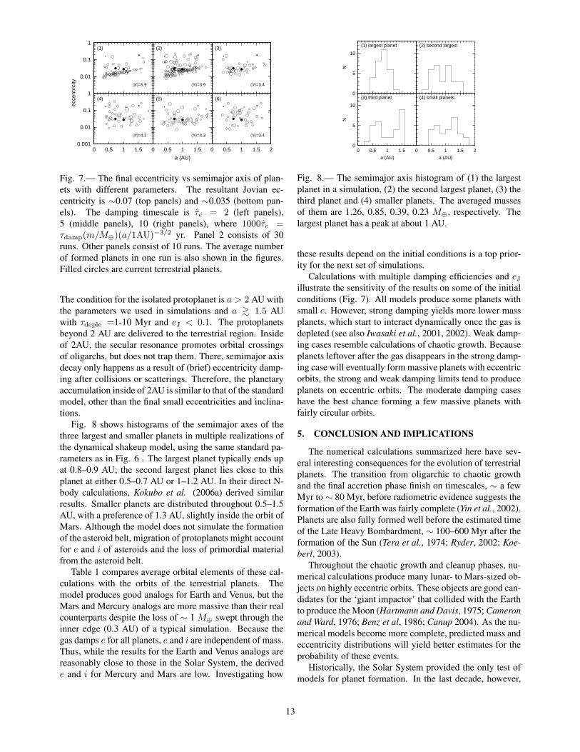
Fig. 7 shows results for multiple 100 Myr calculationswith a variety of initial conditions. The size of the circle isproportional to m1/3. Roughly 75% to 80% of the calcula-tions yield planets with e 0.1. A slightly smaller fraction,∼ 70%, form 3–4 planets. In other simulations, a smallermerger efficiency during the gaseous stage leaves behindmore than 3–4 planets. Some systems become unstable af-ter disk depletion and produce planets with 0.1 e 0.2.Many configurations with more than 5 planets at 100 Myrwill probably develop large e within 1–5 Gyr.

Secular resonant trapping tends to migrate protoplanetsinward with the ν5 resonance (Fig. 6). To maintain resonanttrapping Nagasawa et al. (2005) derived

( a

1AU

)4

26( eJ

0.05

)−2(

m

M⊕

)−1 (tdepl

1Myr

)−1

. (21)

12

0.01

0.1

1

ecce

ntric

ity

(1)

⟨N⟩=5.9

(2)

⟨N⟩=3.9

(3)

⟨N⟩=3.4

0.001

0.01

0.1

1

0 0.5 1 1.5

(4)

⟨N⟩=4.2

0 0.5 1 1.5

a (AU)

(5)

⟨N⟩=4.3

0 0.5 1 1.5 2

(6)

⟨N⟩=3.4

Fig. 7.— The final eccentricity vs semimajor axis of plan-ets with different parameters. The resultant Jovian ec-centricity is ∼0.07 (top panels) and ∼0.035 (bottom pan-els). The damping timescale is τe = 2 (left panels),5 (middle panels), 10 (right panels), where 1000τe =τdamp(m/M⊕)(a/1AU)−3/2 yr. Panel 2 consists of 30runs. Other panels consist of 10 runs. The average numberof formed planets in one run is also shown in the figures.Filled circles are current terrestrial planets.

The condition for the isolated protoplanet is a > 2 AU withthe parameters we used in simulations and a 1.5 AUwith τdeple =1-10 Myr and eJ < 0.1. The protoplanetsbeyond 2 AU are delivered to the terrestrial region. Insideof 2AU, the secular resonance promotes orbital crossingsof oligarchs, but does not trap them. There, semimajor axisdecay only happens as a result of (brief) eccentricity damp-ing after collisions or scatterings. Therefore, the planetaryaccumulation inside of 2AU is similar to that of the standardmodel, other than the final small eccentricities and inclina-tions.

Fig. 8 shows histograms of the semimajor axes of thethree largest and smaller planets in multiple realizations ofthe dynamical shakeup model, using the same standard pa-rameters as in Fig. 6 . The largest planet typically ends upat 0.8–0.9 AU; the second largest planet lies close to thisplanet at either 0.5–0.7 AU or 1–1.2 AU. In their direct N-body calculations, Kokubo et al. (2006a) derived similarresults. Smaller planets are distributed throughout 0.5–1.5AU, with a preference of 1.3 AU, slightly inside the orbit ofMars. Although the model does not simulate the formationof the asteroid belt, migration of protoplanets might accountfor e and i of asteroids and the loss of primordial materialfrom the asteroid belt.

Table 1 compares average orbital elements of these cal-culations with the orbits of the terrestrial planets. Themodel produces good analogs for Earth and Venus, but theMars and Mercury analogs are more massive than their realcounterparts despite the loss of ∼ 1 M⊕ swept through theinner edge (0.3 AU) of a typical simulation. Because thegas damps e for all planets, e and i are independent of mass.Thus, while the results for the Earth and Venus analogs arereasonably close to those in the Solar System, the derivede and i for Mercury and Mars are low. Investigating how

0

5

10

N

(1) largest planet (2) second largest

0

5

10

0 0.5 1 1.5

N

a (AU)

(3) third planet

0 0.5 1 1.5 2

a (AU)

(4) small planets

Fig. 8.— The semimajor axis histogram of (1) the largestplanet in a simulation, (2) the second largest planet, (3) thethird planet and (4) smaller planets. The averaged massesof them are 1.26, 0.85, 0.39, 0.23 M⊕, respectively. Thelargest planet has a peak at about 1 AU.

these results depend on the initial conditions is a top prior-ity for the next set of simulations.

Calculations with multiple damping efficiencies and eJ

illustrate the sensitivity of the results on some of the initialconditions (Fig. 7). All models produce some planets withsmall e. However, strong damping yields more lower massplanets, which start to interact dynamically once the gas isdepleted (see also Iwasaki et al., 2001, 2002). Weak damp-ing cases resemble calculations of chaotic growth. Becauseplanets leftover after the gas disappears in the strong damp-ing case will eventually form massive planets with eccentricorbits, the strong and weak damping limits tend to produceplanets on eccentric orbits. The moderate damping caseshave the best chance forming a few massive planets withfairly circular orbits.

5. CONCLUSION AND IMPLICATIONS

The numerical calculations summarized here have sev-eral interesting consequences for the evolution of terrestrialplanets. The transition from oligarchic to chaotic growthand the final accretion phase finish on timescales, ∼ a fewMyr to ∼ 80 Myr, before radiometric evidence suggests theformation of the Earth was fairly complete (Yin et al., 2002).Planets are also fully formed well before the estimated timeof the Late Heavy Bombardment, ∼ 100–600 Myr after theformation of the Sun (Tera et al., 1974; Ryder, 2002; Koe-berl, 2003).

Throughout the chaotic growth and cleanup phases, nu-merical calculations produce many lunar- to Mars-sized ob-jects on highly eccentric orbits. These objects are good can-didates for the ‘giant impactor’ that collided with the Earthto produce the Moon (Hartmann and Davis, 1975; Cameronand Ward, 1976; Benz et al, 1986; Canup 2004). As the nu-merical models become more complete, predicted mass andeccentricity distributions will yield better estimates for theprobability of these events.

Historically, the Solar System provided the only test ofmodels for planet formation. In the last decade, however,

13

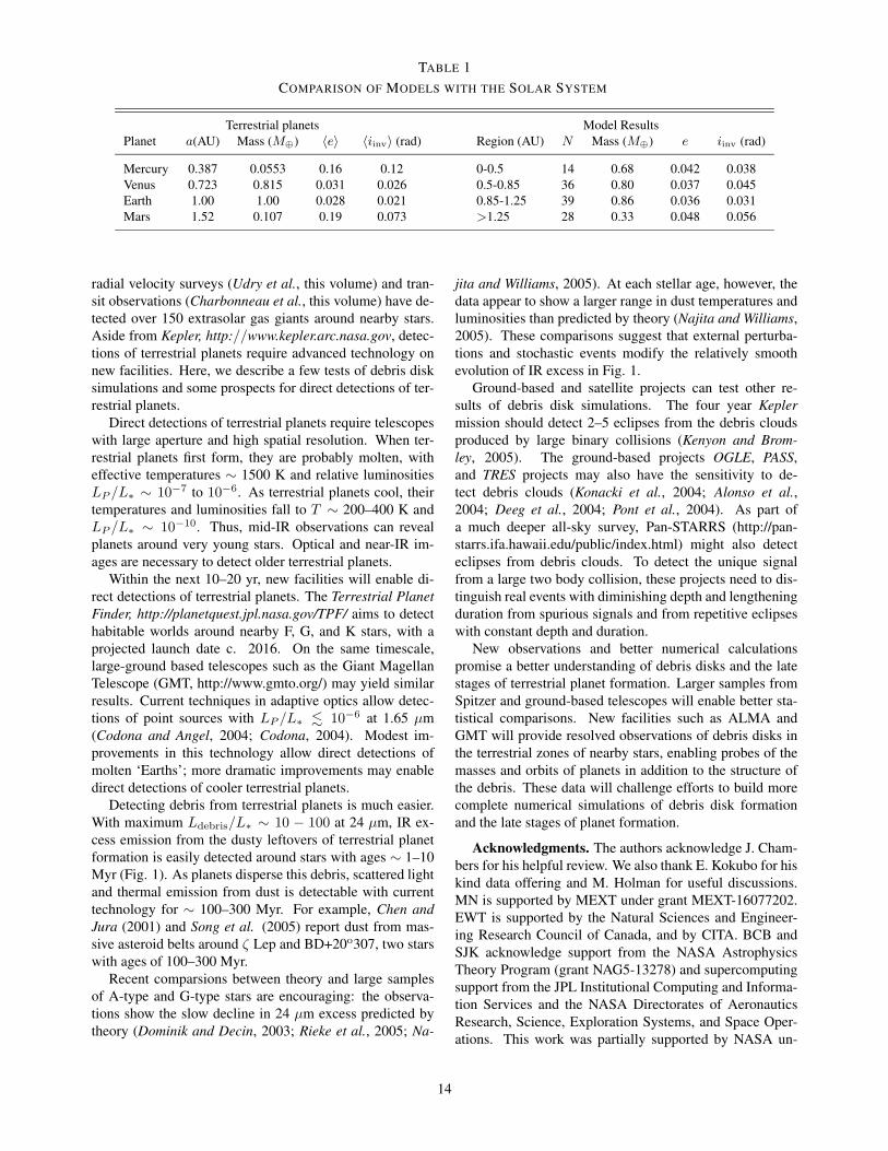
TABLE 1COMPARISON OF MODELS WITH THE SOLAR SYSTEM

Terrestrial planets Model ResultsPlanet a(AU) Mass (M⊕) 〈e〉 〈iinv〉 (rad) Region (AU) N Mass (M⊕) e iinv (rad)

Mercury 0.387 0.0553 0.16 0.12 0-0.5 14 0.68 0.042 0.038Venus 0.723 0.815 0.031 0.026 0.5-0.85 36 0.80 0.037 0.045Earth 1.00 1.00 0.028 0.021 0.85-1.25 39 0.86 0.036 0.031Mars 1.52 0.107 0.19 0.073 >1.25 28 0.33 0.048 0.056

radial velocity surveys (Udry et al., this volume) and tran-sit observations (Charbonneau et al., this volume) have de-tected over 150 extrasolar gas giants around nearby stars.Aside from Kepler, http://www.kepler.arc.nasa.gov, detec-tions of terrestrial planets require advanced technology onnew facilities. Here, we describe a few tests of debris disksimulations and some prospects for direct detections of ter-restrial planets.

Direct detections of terrestrial planets require telescopeswith large aperture and high spatial resolution. When ter-restrial planets first form, they are probably molten, witheffective temperatures ∼ 1500 K and relative luminositiesLP /L∗ ∼ 10−7 to 10−6. As terrestrial planets cool, theirtemperatures and luminosities fall to T ∼ 200–400 K andLP /L∗ ∼ 10−10. Thus, mid-IR observations can revealplanets around very young stars. Optical and near-IR im-ages are necessary to detect older terrestrial planets.

Within the next 10–20 yr, new facilities will enable di-rect detections of terrestrial planets. The Terrestrial PlanetFinder, http://planetquest.jpl.nasa.gov/TPF/ aims to detecthabitable worlds around nearby F, G, and K stars, with aprojected launch date c. 2016. On the same timescale,large-ground based telescopes such as the Giant MagellanTelescope (GMT, http://www.gmto.org/) may yield similarresults. Current techniques in adaptive optics allow detec-tions of point sources with LP /L∗ 10−6 at 1.65 µm(Codona and Angel, 2004; Codona, 2004). Modest im-provements in this technology allow direct detections ofmolten ‘Earths’; more dramatic improvements may enabledirect detections of cooler terrestrial planets.

Detecting debris from terrestrial planets is much easier.With maximum Ldebris/L∗ ∼ 10 − 100 at 24 µm, IR ex-cess emission from the dusty leftovers of terrestrial planetformation is easily detected around stars with ages ∼ 1–10Myr (Fig. 1). As planets disperse this debris, scattered lightand thermal emission from dust is detectable with currenttechnology for ∼ 100–300 Myr. For example, Chen andJura (2001) and Song et al. (2005) report dust from mas-sive asteroid belts around ζ Lep and BD+20o307, two starswith ages of 100–300 Myr.

Recent comparsions between theory and large samplesof A-type and G-type stars are encouraging: the observa-tions show the slow decline in 24 µm excess predicted bytheory (Dominik and Decin, 2003; Rieke et al., 2005; Na-

jita and Williams, 2005). At each stellar age, however, thedata appear to show a larger range in dust temperatures andluminosities than predicted by theory (Najita and Williams,2005). These comparisons suggest that external perturba-tions and stochastic events modify the relatively smoothevolution of IR excess in Fig. 1.

Ground-based and satellite projects can test other re-sults of debris disk simulations. The four year Keplermission should detect 2–5 eclipses from the debris cloudsproduced by large binary collisions (Kenyon and Brom-ley, 2005). The ground-based projects OGLE, PASS,and TRES projects may also have the sensitivity to de-tect debris clouds (Konacki et al., 2004; Alonso et al.,2004; Deeg et al., 2004; Pont et al., 2004). As part ofa much deeper all-sky survey, Pan-STARRS (http://pan-starrs.ifa.hawaii.edu/public/index.html) might also detecteclipses from debris clouds. To detect the unique signalfrom a large two body collision, these projects need to dis-tinguish real events with diminishing depth and lengtheningduration from spurious signals and from repetitive eclipseswith constant depth and duration.

New observations and better numerical calculationspromise a better understanding of debris disks and the latestages of terrestrial planet formation. Larger samples fromSpitzer and ground-based telescopes will enable better sta-tistical comparisons. New facilities such as ALMA andGMT will provide resolved observations of debris disks inthe terrestrial zones of nearby stars, enabling probes of themasses and orbits of planets in addition to the structure ofthe debris. These data will challenge efforts to build morecomplete numerical simulations of debris disk formationand the late stages of planet formation.

Acknowledgments. The authors acknowledge J. Cham-bers for his helpful review. We also thank E. Kokubo for hiskind data offering and M. Holman for useful discussions.MN is supported by MEXT under grant MEXT-16077202.EWT is supported by the Natural Sciences and Engineer-ing Research Council of Canada, and by CITA. BCB andSJK acknowledge support from the NASA AstrophysicsTheory Program (grant NAG5-13278) and supercomputingsupport from the JPL Institutional Computing and Informa-tion Services and the NASA Directorates of AeronauticsResearch, Science, Exploration Systems, and Space Oper-ations. This work was partially supported by NASA un-

14

der grant NAGS5-11779 and NNG04G-191G, by JPL un-der grant 1228184, and by NSF under grant AST-9987417through DNCL.

REFERENCES

Abe Y., Ohtani E., Okuchi T., Righter K., and Drake M. (2000) InOrigin of the Earth and Moon (R. M. Canup and K. Righter,eds.), Univ. of Arizona, Tucson, p. 413-433.

Adachi I., Hayashi C., and Nakazawa K. (1976) Prog. Theor.Phys., 56, 1756-1771.

Agnor C. B., Canup R. M., and Levison H. F. (1999) Icarus, 142,219-237.

Agnor C. B. and Ward W. R. (2002) Astrophys. J., 567, 579-586.Agnor C. and Asphaug E. (2004) Astrophys. J., 613, L157-L160.Alonso R., Brown T., Torres G., Latham D. W., Sozzetti A. et al.

(2004) Astrophys. J., 613, L153-L156.Armitage P. J. (2003) Astrophys. J., 582, L47-L50.Artymowicz P. (1993) Astrophys. J., 419, 166-180.Balsiger H., Altwegg K., and Geiss J. (1995) Jour. Geophys. Res.,

100, 5827-5834.Barbieri M., Marzari F., and Scholl H. (2002) Astron. Astrophys.,

396, 219-224.Butler R. P., Marcy G. W., Fischer D. A., Brown T. M., Contos A.

R. et al. (1999) Aastrophys. J., 526, 916-927.Benz W. and Asphaug E. (1999) Icarus, 142, 5-20.Benz W., Slattery W. L., and Cameron A. G. W. (1986) Icarus, 66,

515-535.Bockelee-Morvan D., Gautier D., Lis D. C., Young K., Keene J. et

al. (1998) Icarus, 133, 147-162.Bromley B. C. and Kenyon S. J. (2006) Astron. J., in press.Cameron A. G. W. and Ward W. R. (1976) Abst. Lunar Planetary

Sci. Conf., 7, 120-120.Canup R. (2004) Ann. Rev. Astron. Astrophys., 42, 441-475.Chambers J. E. (2001) Icarus, 152, 205-224.Chambers J. E. and Cassen P. (2002) Meteoritics & Planet. Sci.,

37, 1523-1540.Chambers J. E. and Wetherill G. W. (1998) Icarus, 136, 304-327.Chambers J. E., Wetherill G. W., and Boss A. P. (1996) Icarus,

119, 261-268.Chen C. H. and Jura M. (2001) Astrophys. J., 560, L171-L174.Codona J. L. (2004) Proc. SPIE, 5490, 379-388.Codona J. L. and Angel R. (2004) Astrophys. J., 604, L117-L120.Cox L. P. and Lewis J. S. (1980) Icarus, 44, 706-721.Drake M. J. (2005) Meteoritics & Planetary Science, 40, 519-527.Drake M. J. and Righter K. (2002) Nature, 416, 39-44.Dauphas N., Robert F., and Marty B. (2000) Icarus, 148, 508-512.Deeg H. J., Alonso R., Belmonte J. A., Alsubai K., Horne K. et al.

(2004) Publ. Astron. Soc. Pac., 116, 985-995.Dominik C. and Decin G. (2003) Astrophys. J., 598, 626-635.Duncan M. J., Levison H. F., and Lee M. H. (1998) Astron. J.,

116, 2067-2077.Durda D. D., Greenberg R., and Jedicke R. (1998) Icarus, 135,

431-440.Durda D. D., Bottke W. F., Enke B. L., Merline W. J., Asphaug E.

et al. (2004) Icarus, 170, 243-257.Fogg M. J. and Nelson R. P. (2005) Astron. Astrophys., 441, 791-

806.Goldreich P., Lithwick Y., and Sari R. (2004) Ann. Rev. Astron.

Astrophys., 42, 549-601.Goldreich P. and Tremaine S. (1980), Astrophys. J., 241, 425-441.

Goldreich P. and Ward W. R. (1973) Astrophys. J., 183, 1051-1062.

Gomes R., Levison H. F., Tsiganis K., and Morbidelli A. (2005)Nature, 435, 466-469

Greenberg R., Hartmann W. K., Chapman C. R., and Wacker J. F.(1978) Icarus, 35, 1-26.

Grogan K., Dermott S. F., and Durda D. D. (2001) Icarus, 152,251-267.

Halliday A. N. (2004) Nature, 427, 505-590.Halliday A. N., Lee D-C., and Jacobsen S. B. (2000) In Origin of

the Earth and Moon (R. M. Canup and K. Righter, eds.), pp.45-62. Univ. of Arizona, Tucson.

Hayashi C. (1981) Prog. Theor. Phys. Suppl., 70, 35-53.Hayashi C., Nakazawa K., and Nakagawa Y. (1985) In Protostars

and planets II (D. C. Black and M. S. Matthews, eds.), pp.1100-1153. Univ. of Arizona, Tucson.

Hartmann W. K. and Davis D. R. (1975), Icarus, 24, 504-514.Heppenheimer T. A. (1978) Astron. Astrophys., 65, 421-426.Holsapple K. L (1994) Planet. Space Sci., 42, 1067-1078.Housen K. and Holsapple K. (1990) Icarus, 84, 226-253.Housen K. and Holsapple K. (1999) Icarus, 142, 21-33.Ida S. and Makino J. (1993) Icarus, 106, 210-227. 875-889.Inaba S., Tanaka H., Nakazawa K., Wetherill G. W., and Kokubo

E. (2001) Icarus, 149, 235-250.Ito T. and Tanikawa K. (1999) Icarus, 139, 336-349.Iwasaki K., Tanaka H., Nakazawa K., and Emori H. (2001) Publ.

Astron. Soc. Japan, 53, 321-329.Iwasaki K., Emori H., Nakazawa K., and Tanaka H. (2002) Publ.

Astron. Soc. Japan, 54, 471-479.Jacobsen S. B. (2005) Ann. Rev. Earth Planet. Sci., 33, 531-570.Jones B. W., Sleep P. N., and Chambers J. E. (2001) Astronomy

Astrophys., 366, 254-262Kenyon S. J. and Bromley B. C. (2002) Astrophys. J., 577, L35-

L38.Kenyon S. J. and Bromley B. C. (2004a) Astron. J., 127, 513-530.Kenyon S. J. and Bromley B. C. (2004b) Astrophys. J., 602, L133-

L136.Kenyon S. J. and Bromley B. C. (2005) Astron. J., 130, 269-279.Kenyon S. J. and Bromley B. C. (2006) Astron. J., 131, No. 3.Kenyon S. J. and Hartmann L. W. (1995) Astrophys. J. Suppl.,

101, 117-171.Koeberl C. (2003) Earth Moon Planets, 92, 79-87.Kokubo E. and Ida S. (1995) Icarus, 114, 247-257.Kokubo E. and Ida S. (1996) Icarus, 123, 180-191.Kokubo E. and Ida S. (1998) Icarus, 131, 171-178.Kokubo E. and Ida S. (2000) Icarus, 143, 15-27.Kokubo E. and Ida S. (2002) Astrophys. J., 581, 666-680.Kokubo E., Kominami J., and Ida S. (2006a), Astrophys. J. ac-

cepted.Kominami J. and Ida S. (2002) Icarus, 157, 43-56.Kominami J. and Ida S. (2004) Icarus, 167, 231-243.Konacki M., Torres G., Sasselov D. D., Pietrzyski G., Udalski A.

et al. (2004) Astrophys. J., 609, L37-L40.Kortenkamp S. J. and Wetherill G. W. (2000) Icarus, 143, 60-73.Kortenkamp S. J., Kokubo E., and Weidenschilling S. J. (2000) In

Origin of the Earth and Moon (R. M. Canup and K. Righter,eds.), pp. 75-84. Univ. of Arizona, Tucson.

Kortenkamp S. J., Wetherill G. W., and Inaba S. (2001) Science,293, 1127-1129.

Laughlin G., Chambers J., and Fischer D. (2002) Astrophys. J.,579, 455-467.

Lecar M. and Aarseth S. J. (1986) Astrophys. J., 305, 564-579.

15

Levison H. F. and Agnor C. (2003) Astron. J., 125, 2692-2713.Levison H. F., Dones L., Chapman C. R., Stern S. A., Duncan

M. J., and Zahnle, K. (2001) Icarus, 151, 286-306.Leinhardt Z. M. and Richardson D. C. (2005) Astrophys. J., 625,

427-440.Lissauer J. J. (1987) Icarus, 69, 249-265.Lissauer J. J. and Kary D. M. (1991) Icarus, 94, 126-159.Lissauer J. J. and Stewart G. R. (1993) In Protostars and Planets

III (E. H. Levy and J. J. Lunine, eds.), pp. 1061-1088. Univ. ofArizona, Tucson.

Lunine J. I., Chambers J., Morbidelli A., and Leshin L. A. (2003)Icarus, 165, 1-8.

Marcy G. W., Butler R. P., Fischer D. A., and Vogt S. S. (2004)In Extrasolar Planets: Today and Tomorrow (J. P. Beaulieu, E.A. Lecavelier, and C. Terquem, eds.), pp. 3-14. Astron. Soc.Pacific, San Francisco.

Marzari F. and Scholl, H. (2000) Astrophys. J., 543, 328-339.Mayor M. and Queloz D. (1995) Nature, 378, 355-359.Mayor M., Udry S., Naef D., Pepe F., Queloz D. et al. (2004)

Astron. Astrophys., 415, 391-402.McArthur B. E., Endl M., Cochran W. D., Benedict G. F., Fischer

D. A. et al. (2004) Astrophys. J., 614, L81-L84.McNeil D., Duncan M. J., and Levison H. F. (2005), Astron J.,

130, 2884-2899.Meier R., Owen T. C., Jewitt D, C., Matthews H. E., Senay M. et

al. (1998) Science, 279, 1707-1710.Michel P., Benz W., Tanga P., and Richardson D. C. (2001)Sci-

ence, 294, 1696-1700.Morbidelli A., Chambers J., Lunine J. I., Petit J. M., Robert F. et

al. (2000) Meteoritics & Planet. Sci., 35, 1309-1320.Nagasawa M., Tanaka H., and Ida S. (2000) Astron. J., 119, 1480-

1497.Nagasawa M., Lin D. N. C., and Thommes E. (2005) Astrophys.

J., 635, 578-598.Najita J. and Williams J. P. (2005) Astrophys. J., 635, 625-635.Ohtsuki K., Ida S., Nakagawa Y., and Nakazawa K. (1993) In Pro-

tostars and Planets III (E. H. Levy and J. I. Lunine, eds.), pp.1089-1107. Univ. of Arizona, Tucson.

Ohtsuki K., Stewart G. R., and Ida S. (2002) Icarus, 155, 436.Pollack J. B., Hubickyj O., Bodenheimer P., Lissauer J. J., Podolak

M. et al. (1996) Icarus, 124, 62-85.Pont F., Bouchy F., Queloz D., Santos N. C., Melo C. et al. (2004)

Astron. Astrophys., 426, L15-L18.Quintana E. V., Lissauer J. J., Chambers J. E., and Duncan M.

(2002) Astrophys. J., 576, 982-996.Raymond S. N., Quinn T., and Lunine J. I. (2004) Icarus, 168,

1-17.Raymond S. N., Quinn, T., and Lunine J. I. (2005a) Astrophys. J.,

632, 670-676.Raymond S. N., Quinn T,, and Lunine J. I. (2005b) Icarus, 177,

256-263.Rieke G. H., Su K. Y. L., Stansberry J. A., Trilling D., Bryden G.

et al. (2005) Astrophys. J., 620, 1010-1026.Ryder G. (2002) Journ. Geophys. Res., 107, 6-26.Safronov V. (1969) In Evolution of the Protoplanetary Cloud and

Formation of the Earth and Planets, Nauka Press, Moscow.Sasaki T. and Abe Y. (2005) In PPV Poster Proceedings

http://www.lpi.usra.edu/meetings/ppv2005/pdf/8221.pdfSong I., Zuckerman B., Weinberger A. J., and Becklin E. E. (2005)

Nature, 436, 363-365.Tanaka H. and Ida S. (1999) Icarus, 139, 350-366.Tanaka H. and Ward W. R. (2004) Astrophys. J., 602, 388-395.

Tanaka H., Takeuchi T., and Ward W. R. (2002) Astrophys. J., 565,1257-1274.

Tera F., Papanastassiou D. A., and Wasserburg G. J. (1974) EarthPlanet. Sci., 22, L1-L21.

Thebault P., Marzari F., and Scholl H. (2002) Astron. Astrophys.,384, 594-602.

Ward W. R. (1973) Science, 181, 260-262.Ward W. R. (1981) Icarus, 47, 234-264.Ward W. R. (1986) Icarus, 67, 164-180.Ward W. R. (1989) Astrophys. J., 345, L99-L102.Ward W. R. (1993) Icarus, 106, 274-287.Ward W. R. (2000) In Origin of the Earth and Moon (R. M. Canup

and K. Righter, eds.), pp. 75-84. Univ. of Arizona, Tucson.Ward, W. R., Colombo, G., and Franklin, F. A. (1976), Icarus, 28,

441-452.Weidenschiling S. J. (1995) Icarus, 116, 433-435.Weidenschilling S. J. and Cuzzi J. N. (1993) In Protostars and

Planets III (E. H. Levy and J. J. Lunine, eds.), pp. 1031-1060.Univ. of Arizona, Tucson.

Weidenschilling, S. J., Spaute, D., Davis, D. R., Marzari, F., andOhtsuki, K. (1997) Icarus, 128, 429-455.

Wetherill, G. W. (1980) Ann. Rev. Astron. Astrophys., 18, 77-113.Wetherill G. W. (1985) Science, 228, 877-879.Wetherill, G. W. (1990) Icarus, 88, 336-354.Wetherill G. W. (1996) Icarus, 119, 219-238.Wetherill G. W. and Stewart G. R. (1989) Icarus, 77, 330-357.Wetherill G. W. and Stewart G. R. (1993) Icarus, 106, 190-209.Wood B. J. and Halliday A. N. (2005) Nature, 437, 1345-1348.Yin Q., Jacobsen S. B., Yamashita K., Blichert-Toft J., Telouk P.

et al. (2002) Nature, 418, 949-952.Youdin A. N. and Shu F. H (2002) Astrophys. J., 580, 494-505.Zhou J.-L., Asrseth S. J., Lin D. N. C., and Nagasawa M. (2005)Astrophys. J., 631, L85-L88.

16