Temperature dependence ofthe band emittance for nongray bodies

Orjan Staaf, Carl G. Ribbing, and Stefan K. Andersson

The general problem of obtaining correct emittance values from broadband IR radiometric measurementson nongray samples is discussed. If the spectral emittance has structure in a band, the emittance,averaged over that band, will be temperature dependent, even if the spectral emittance is insensitive tothe temperature change. We point out that a widely used expression, with correction for radiance fromthe surroundings reflected by the sample, is valid only if the spectral emittance is temperature andwavelength independent, i.e., gray. If the spectral emittance is nongray, the conventional emissionfactor, as determined by a broadband radiometer, is temperature dependent and the numerical value issignificantly different from the averaged band emittance sought. Two algorithms are suggested toextract the correct band-averaged emittance from the temperature-dependent radiometric emissionfactor obtained with the conventional expression. The algorithms are demonstrated with a step modelfor the spectral emittance, and it is shown that the agreement with the correct average band emittanceis significantly improved. © 1996 Optical Society of America

Key words: Radiometry, emission factor, emittance, thermal emission, temperature dependence.

1. Introduction

Amultitude of applications for broadband radiometryexists, e.g., in remote sensing, medical examination,power distribution diagnostics, solar-system evalua-tion, andmilitary reconnaissance.1,2 In the simplestversion a pyrometer system is used to determine thetemperature of a hot source. Here hot exhaustplume radiation is not considered. More advancedinstruments are designed to give an image in whichthe contrast is created by variations in radiance fromthe different pixels of the image. If the radiatingobject is one flat piece of the same material, one canuse the image as a representation of surface-temperature variations across the sample. If the ob-ject is more complex, one has to consider the influenceof the surface emittance. Contrast may appear be-cause different parts of the object surface have differ-ent emittance values as well as from temperaturedifferences.Assuming that the detector system has well-

O. Staaf and C. G. Ribbing are with Division 63, National De-fense Research Establishment, S-172 90 Stockholm, Sweden.S. K. Andersson is with the Department of Technology, Solid StatePhysics, Box 534, Uppsala University, S-175 21 Uppsala, Sweden.Received 27 November 1995; revised manuscript received 17

June 1996.0003-6935y96y316120-06$10.00y0© 1996 Optical Society of America

6120 APPLIED OPTICS y Vol. 35, No. 31 y 1 November 1996

determined wavelength limits, a and b, we can for-mally express the emitted radiance Le recorded byour system as

Le~a, b, T! 5 *a

b

ε~l!Lbb~l, T!dl, (1)

where Lbb is the Planck function and ε~l! is the spec-tral emittance. In the most general case the spec-tral emittance ~and the bulk reflectance! is a functionof temperature, ε~l, T!. As long as the temperatureis well below the Debye temperature of the sampleand the temperature change is small, this variationcan be neglected, and we shall do so henceforth. Thedual source of contrast in Eq. ~1! is the origin of onebasic difficulty in radiometricmeasurements. To de-termine the emittance of an object with a radiometer,one must know the surface temperature, and to de-termine the surface temperature radiatively, we needthe emittance. Many arrangements and methodshave been worked out to solve this difficulty.3The spectral emittance is a dimensionless number

between 0 and 1, and it is mathematically obviousthat an average emittance valid for the wavelengthinterval @a, b# exists. A complete symbol should in-clude this integration interval, ε#~T, a, b!, but we shalluse the symbol ε# where no confusion can arise. This

average quantity

ε#~T! 5

*a

b

ε~l!Lbb~l, T!dl

*a

b

Lbb~l, T!dl

, (2)

which can equally well be calculated in energy orwave-number space, is often used in various applica-tions of thermal IR radiometry. It appears from thisdefinition that ε#~T! is temperature dependent, even ifthe thermal dependence of the spectral emittance ε~l!is negligible. In Fig. 1 this point is further elabo-rated. It shows two Planck curves for temperatures,T1 , T2, and two model emittance spectra, one grayand one with a step structure on a common wave-length axis. As explained in the Fig. 1 caption it isobvious that the folding operation carried out whenthe average of Eq. ~2! is calculated will give ε#~T1! 5ε#~T2! for the gray case, but this will not be true whenthe emittance features spectral variation within theradiometer detection range, as the step model, 2,does.One main purpose of this research is to show that

this temperature variation is significant in somecases of interest, a variation that has so far beenneglected in the practical analysis of radiometer data.We shall also demonstrate some methods that can beused to handle this variation and derive an approxi-mately correct emittance value from the experimen-tal results when the spectral function ε~l! isunknown.Before going into the details of the temperature

dependence, we must deal with another complicationin thermal radiometry. If the object is not muchwarmer than the ambient, we cannot neglect, as wasdone in Eq. ~1!, the radiation emitted by the sur-

Fig. 1. Two-model emittance spectra and Planck curves for twotemperatures, demonstrating the temperature dependence of bandemittance. A change in temperature redistributes the weights ofthe Planck function, which changes the average ε# even though ε~l!is assumed to be temperature independent. Also indicated is thedetector sensitivity range, a 5 7.7 and b 5 13.0 mm. The graymodel, 1, is a constant, ε1 5 0.5, and the step function model, 2,drops from ε2 5 0.9 to ε2 5 0.1 at the wavelength, c 5 10 mm.

roundings and then reflected by the object. It is wellknown that the reflectance R of an opaque body issimply related to the emittance:4 R 5 1 2 ε, whichgives the correction term directly for the reflectedintensity:

Lr~Ta! 5 *a

b

@1 2 ε~l!#Lbb~l, Ta!dl. (3)

It is essential that the temperature Ta in Eq. ~3! is thetemperature of the ambient, which is not the same asthat of the sample. For quantitative applications itis an advantage that the temperature of the sur-roundings is as uniform as possible; otherwise the Lbbfunction in Eq. ~3! must be evaluated at a suitableaverage temperature. Note that in Eq. ~3! we as-sume that the effective emittance of the surroundingsis unity, i.e., a perfect blackbody. This is not asrestrictive as it may appear, however. For a similarreason that the physical realization of a perfect black-body is a Holeraum, it suffices that the effective areaof the surroundings is much larger than that of thesample. In practice one should strive for a homoge-neous background with sufficient distance from theobject. Practitioners of thermal imaging also avoidperpendicular observation of the sample, because thiscauses a cold reflection of the camera–lens system.Combining Eqs. ~1!–~3!, we obtain an equation for

the total radiance LA seen by the imaging system.The integration interval is implicit for this symbol:

LA~T, Ta! 5 ε#~T! *a

b

Lbb~l, T!dl

1 @1 2 ε#~Ta!# *a

b

Lbb~l, Ta!dl. (4)

Contemplating Eq. ~4!, we realize that only if thesample temperature is much higher than that of thesurroundings andyor if the sample emittance is '1,can the second term, i.e., the reflectance correction,be neglected. This implies that from the value of LAalone one cannot extract the ε# value. Equation ~4!is, however, the basis for the conventional analysis ofa general case when the reflectance of thermal radi-ation from the surroundings must be considered andadditional measurements are required for the deter-mination of the sample emittance.In Section 2 we shall first recapitulate this conven-

tional formalism, which takes account of the reflectedradiance but neglects the temperature variation ofthe emittance. We shall demonstrate that the latterleads to an error in the numerical value of the emit-tance. This is illustrated with the model emittancespectra in Fig. 1. In Section 2 also we shall intro-duce algorithms that approximately include this tem-perature variation and give an improved value for thesample emittance.These results are not without practical signifi-

cance. We have previously pointed out that the rest-strahlen band of beryllium oxide can be used to

1 November 1996 y Vol. 35, No. 31 y APPLIED OPTICS 6121

obtain selective low emittance in the upper atmo-spheric window, 7.7–13 mm.5 In this case the ther-mal effects are significant because the BeOreststrahlen band corresponds to a strong spectralfeature in the window.

2. Formalism

In practice, the technique used to account for theeffects of reflected thermal radiation is to make twoextra radiance measurements, one on a blackbody atthe same temperature as the sample for calibrationand one on a representative spot of the surroundings.The radiance levels, LB and LC, with notations asabove will then be

LB~T! 5 *a

b

Lbb~l, T!dl, (5)

LC~Ta! 5 *a

b

Lbb~l, Ta!dl. (6)

Note that Eq. ~6! does not imply that the surround-ings are perfectly black. The radiance, LC as well asLA, is the sum of an emitted and a reflected contri-bution that add up to Eq. ~6! if both contributionsoriginate from surfaces with the same temperature.It is Eq. ~6! that constitutes the requirement of ther-mal homogeneity of the laboratory surroundings.Using Eqs. ~5! and ~6! in Eq. ~4!, we obtain

LA~T, Ta! 5 ε#~T!LB~T! 1 @1 2 ε#~Ta!#LC~Ta!. (7)

As seen, the extra measured L values relate the sam-ple emittance that we wish to determine to the totalradiance from the sample that is primarilymeasured.We now reach the crucial point, at which the temper-ature dependence of the band emittance is neglected,i.e., setting ε#~T! ' ε#~Ta! 5 ^ε&. Then Eq. ~7! can besolved, and we obtain

^ε& 5LA 2 LC

LB 2 LC. (8)

Although this standard expression is derived withthe restriction that the emittance is temperature in-dependent, it has become an almost universally ac-cepted expression for band emittance.1,2,6–13 In thispaper ^ε& is called the radiometric emission factor.As mentioned above, the band emittance is in factonly temperature independent if the spectral emit-tance is gray and temperature independent, i.e., onlyif ε~l, T! is constant. Furthermore it should be ob-served that the radiometric emission factor ^ε& de-pends on the ambient temperature; consequently it isnot purely a material property.To illustrate these points, we use the model emit-

tance spectra in Fig. 1 to calculate ε# and ^ε& as func-tions of temperature with the assumption that thespectral emittance ε~l! is temperature independentand the ambient temperature Ta 5 20 °C. In con-trast to ε#, which is well defined at all temperatures,^ε& diverges for T5 Tawhen LA 5 LB 5 LC. This can

6122 APPLIED OPTICS y Vol. 35, No. 31 y 1 November 1996

be understood as a mathematical consequence of thethermodynamic requirement that there should be nonet radiation from an object at the same temperatureas the surroundings. The singularity in ^ε~T!&, how-ever, satisfies the requirement of the rule ofl’Hospital, i.e., lim ^ε& 5 0y0 when T3 Ta, so that wecan use

^ε~Ta!& 5dLAydTdLBydT

(9)

if it has a well-defined value, which in turn is approx-imated by interpolation of Eq. ~8! across Ta.The results are shown in Fig. 2 with model param-

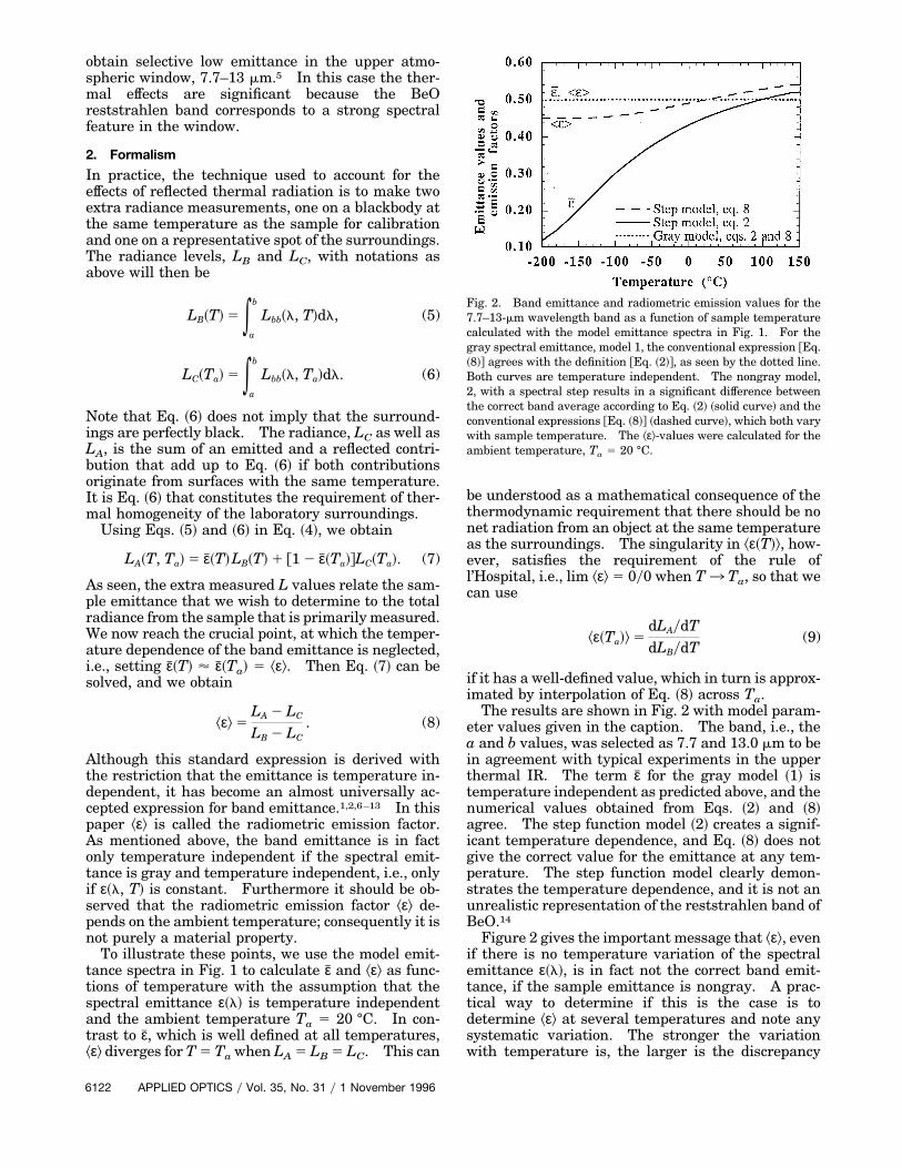
eter values given in the caption. The band, i.e., thea and b values, was selected as 7.7 and 13.0 mm to bein agreement with typical experiments in the upperthermal IR. The term ε# for the gray model ~1! istemperature independent as predicted above, and thenumerical values obtained from Eqs. ~2! and ~8!agree. The step function model ~2! creates a signif-icant temperature dependence, and Eq. ~8! does notgive the correct value for the emittance at any tem-perature. The step function model clearly demon-strates the temperature dependence, and it is not anunrealistic representation of the reststrahlen band ofBeO.14Figure 2 gives the important message that ^ε&, even

if there is no temperature variation of the spectralemittance ε~l!, is in fact not the correct band emit-tance, if the sample emittance is nongray. A prac-tical way to determine if this is the case is todetermine ^ε& at several temperatures and note anysystematic variation. The stronger the variationwith temperature is, the larger is the discrepancy

Fig. 2. Band emittance and radiometric emission values for the7.7–13-mm wavelength band as a function of sample temperaturecalculated with the model emittance spectra in Fig. 1. For thegray spectral emittance, model 1, the conventional expression @Eq.~8!# agrees with the definition @Eq. ~2!#, as seen by the dotted line.Both curves are temperature independent. The nongray model,2, with a spectral step results in a significant difference betweenthe correct band average according to Eq. ~2! ~solid curve! and theconventional expressions @Eq. ~8!# ~dashed curve!, which both varywith sample temperature. The ^ε&-values were calculated for theambient temperature, Ta 5 20 °C.

between ε# and ^ε&. The slope of ^ε~T!& depends on theposition and the magnitude of the structure in thespectral emittance and it is negative if ε~l! increaseswith wavelength, i.e., the opposite to model 2 in Fig.1. Note furthermore that, although the two curvesconverge at high sample temperatures when the re-flected radiation becomes negligible, the results inFig. 2 indicate that quite high sample temperaturesmay be necessary to determine even an approximateε# value with the conventional analysis. In the low-sample-temperature range, ^ε~T!& tails toward a con-stant value, which represents a dominance for thereflected term ~3!. As seen from Eqs. ~7! and ~8!when LB 3 0, this asymptotic value is in fact ε#~Ta!.The temperature necessary to become close to thislimit is quite low, however. Experimentally, the ra-diometer in such a situation works as a broadband IRreflectometer with the surroundings as a lamp, i.e.,much hotter than the sample. Taking such low-temperature radiometric measurements is difficult,however, because of the formation of frost on theemitting surface.With the insights gained from these simple model

considerations, it is natural to ask whether it is at allpossible to extract the correct band emission fromradiometer measurements, if the sample is distinctlynongray and the ambient radiation is not negligible.Even if the three L values have been determinedexperimentally, Eq. ~7! contains two unknowns, ε#~T!and ε#~Ta!, except for T 5 Ta, when LA vanishes. Aremaining possibility is to exploit the informationcontained in the temperature variation of ^ε~T!& toobtain ε#~T!. In any case we can draw a practicalconclusion from the discussion above that if a tem-perature variation of ^ε~T!& is noted, it should be un-derstood as a warning signal that ^ε~T!& is differentfrom ε#~T!.We demonstrate two somewhat different ap-

proaches to the problem of determining ε#, and for thisdiscussion it is convenient to rewrite Eq. ~7! as

ε#~T! 5LA~T, Ta! 2 @1 2 ε#~Ta!#LC~Ta!

LB~T!, (10)

which shows that if we can only find the correct emit-tance value at the ambient temperature Ta, we candetermine it for all other temperatures with the ra-diance values LA~T! and LB~T! as well as the constantLC. We shall use the spectral emittance step modelin Fig. 1 to demonstrate the advantages and difficul-ties with the two algorithms in obtaining ε#~T! from^ε~T!&.

A. Linearizing ^«~T!& and «#~T!

In the first method that we suggest for extracting theband emittance from radiometric measurements, weintroduce approximations of the radiometric emis-sion factor and the emittance:

^ε~T!& 5 ^ε~Ta!& 1 k1~T 2 Ta!, (11)

ε#~T! 5 ε#~Ta! 1 c1~T 2 Ta!. (12)

Note that although the linearization of ^ε~T!& appearsto be well founded in our model calculations, it ismuch less so with ε#~T!. It is obvious in Fig. 2 that^ε~T!& is more linear than ε#~T!. In Eq. ~12! we shalltherefore end up with temperature-dependent coeffi-cients c1~T!.Initially, we consider ^ε~T!&: We interpolate it ac-

cording to Eq. ~9! to obtain ^ε~Ta!& and then determinethe coefficient k1, in both cases by linearization. Ourstepmodel gives ^ε~Ta!& ' 0.499 and k1 ' 3.613 1024

~deg!21. It remains to determine the two parame-ters for ε#~T!, a more complicated task. Using Eq. ~7!and inserting Eq. ~12! in Eq. ~8! give

^ε~T!& 5 ε#~Ta! 1 c1~T 2 Ta!LB~T!

LB~T! 2 LC. (13)

The second term in Eq. ~13! is singular at T 5 Ta forthe same reason as ^ε~T!&. The factor multiplying c1,which is well defined and known at all other temper-atures, can be interpolated across the singularity.Using the values for 10 and 30 °C, we obtain

^ε~Ta!& 5 ε#~Ta! 1 c1t

< 0.499. (14)

From dimensional considerations and by identifyingEq. ~14! with Eq. ~12!, we find that the coefficient t 559.96 is a temperature difference, i.e., equal to T1 2Ta, and conclude that the true band emittancereaches the value ^ε~Ta!& at temperature T1, i.e., at;80 °C. This is a crucial result in the sense that itgives a numerical relation between the two functions,^ε~T!& and ε#~T!. Inspection of Fig. 2 confirms thatthis linearized result is at least approximately cor-rect. We are now in a position to solve the entirefunction ε#~T! with Eqs. ~12! and ~14!:

ε#~T! 5 ^ε~Ta!& 1 c1~T 2 T1!. (15)

Note that the second term is negative for T , 80 °C.It remains to express c1 in known quantities withEqs. ~13! and ~14!:

c1 5k1

LB~T!

LB~T! 2 LC2T1 2 Ta

T 2 Ta

, (16)

where k1 is known from the linearized fit of ^ε~T!&.As mentioned above, Eq. ~16! results in aT-dependent coefficient c1, which is formally incon-sistent with the ansatz @Eq. ~12!# but a natural effectof the nonlinear nature of ε#~T!. In Fig. 3 we comparethe model emittance ε#~T! with the values calculatedaccording to Eqs. ~15! and ~16!. For temperatures ofpractical interest, i.e., T $ 10 °C, the agreement isquite satisfactory less than 0.02 too high and evenbetter at high temperatures. In Fig. 3 we also haveincluded the result of calculations by using Eq. ~10!,which is exact, but by using the approximate valuefor ε#~Ta! that was obtained fromEq. ~14!. The agree-ment with the model values of this curve at normaltemperatures is even better than the linear model

1 November 1996 y Vol. 35, No. 31 y APPLIED OPTICS 6123

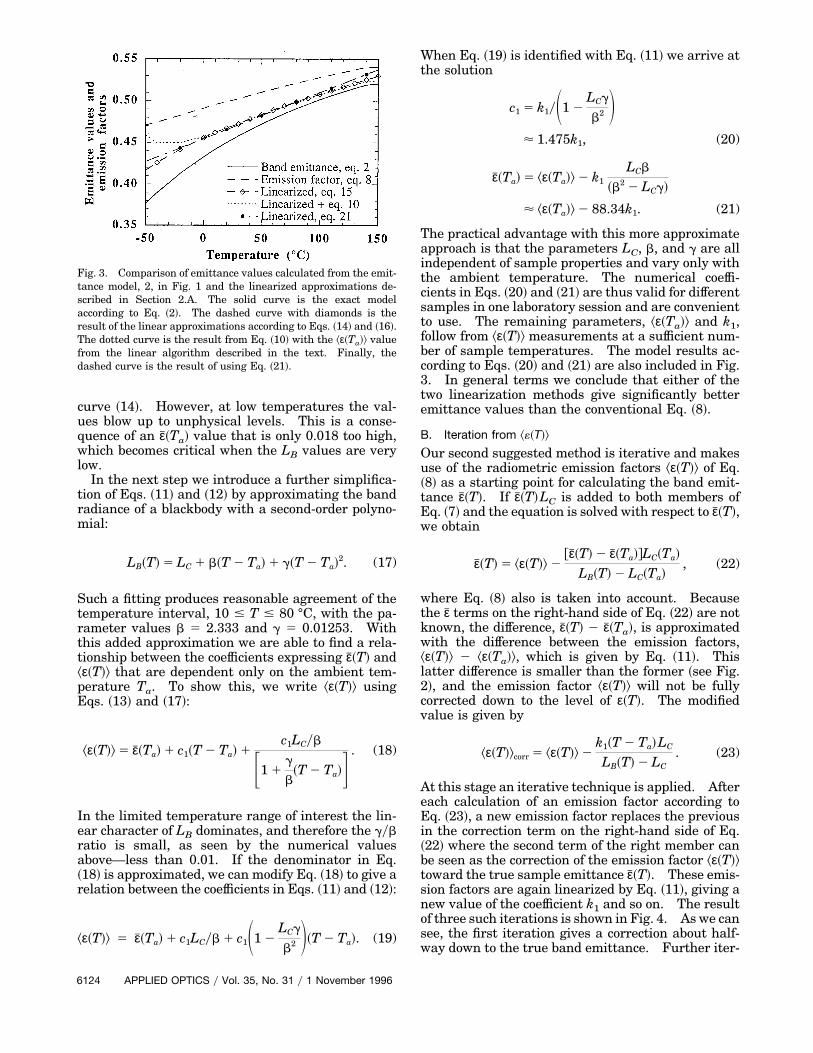
curve ~14!. However, at low temperatures the val-ues blow up to unphysical levels. This is a conse-quence of an ε#~Ta! value that is only 0.018 too high,which becomes critical when the LB values are verylow.In the next step we introduce a further simplifica-

tion of Eqs. ~11! and ~12! by approximating the bandradiance of a blackbody with a second-order polyno-mial:

LB~T! 5 LC 1 b~T 2 Ta! 1 g~T 2 Ta!2. (17)

Such a fitting produces reasonable agreement of thetemperature interval, 10 # T # 80 °C, with the pa-rameter values b 5 2.333 and g 5 0.01253. Withthis added approximation we are able to find a rela-tionship between the coefficients expressing ε#~T! and^ε~T!& that are dependent only on the ambient tem-perature Ta. To show this, we write ^ε~T!& usingEqs. ~13! and ~17!:

^ε~T!& 5 ε#~Ta! 1 c1~T 2 Ta! 1c1LCyb

F1 1g

b~T 2 Ta!G . (18)

In the limited temperature range of interest the lin-ear character of LB dominates, and therefore the gybratio is small, as seen by the numerical valuesabove—less than 0.01. If the denominator in Eq.~18! is approximated, we can modify Eq. ~18! to give arelation between the coefficients in Eqs. ~11! and ~12!:

^ε~T!& 5 ε#~Ta! 1 c1LCyb 1 c1S1 2LCg

b2 D~T 2 Ta!. (19)

Fig. 3. Comparison of emittance values calculated from the emit-tance model, 2, in Fig. 1 and the linearized approximations de-scribed in Section 2.A. The solid curve is the exact modelaccording to Eq. ~2!. The dashed curve with diamonds is theresult of the linear approximations according to Eqs. ~14! and ~16!.The dotted curve is the result from Eq. ~10! with the ^ε~Ta!& valuefrom the linear algorithm described in the text. Finally, thedashed curve is the result of using Eq. ~21!.

6124 APPLIED OPTICS y Vol. 35, No. 31 y 1 November 1996

When Eq. ~19! is identified with Eq. ~11! we arrive atthe solution

c1 5 k1yS1 2LCg

b2 D< 1.475k1, (20)

ε#~Ta! 5 ^ε~Ta!& 2 k1LCb

~b2 2 LCg!

< ^ε~Ta!& 2 88.34k1. (21)

The practical advantage with this more approximateapproach is that the parameters LC, b, and g are allindependent of sample properties and vary only withthe ambient temperature. The numerical coeffi-cients in Eqs. ~20! and ~21! are thus valid for differentsamples in one laboratory session and are convenientto use. The remaining parameters, ^ε~Ta!& and k1,follow from ^ε~T!& measurements at a sufficient num-ber of sample temperatures. The model results ac-cording to Eqs. ~20! and ~21! are also included in Fig.3. In general terms we conclude that either of thetwo linearization methods give significantly betteremittance values than the conventional Eq. ~8!.

B. Iteration from ^«~T!&

Our second suggested method is iterative and makesuse of the radiometric emission factors ^ε~T!& of Eq.~8! as a starting point for calculating the band emit-tance ε#~T!. If ε#~T!LC is added to both members ofEq. ~7! and the equation is solved with respect to ε#~T!,we obtain

ε#~T! 5 ^ε~T!& 2@ε#~T! 2 ε#~Ta!#LC~Ta!

LB~T! 2 LC~Ta!, (22)

where Eq. ~8! also is taken into account. Becausethe ε# terms on the right-hand side of Eq. ~22! are notknown, the difference, ε#~T! 2 ε#~Ta!, is approximatedwith the difference between the emission factors,^ε~T!& 2 ^ε~Ta!&, which is given by Eq. ~11!. Thislatter difference is smaller than the former ~see Fig.2!, and the emission factor ^ε~T!& will not be fullycorrected down to the level of ε~T!. The modifiedvalue is given by

^ε~T!&corr 5 ^ε~T!& 2k1~T 2 Ta!LC

LB~T! 2 LC. (23)

At this stage an iterative technique is applied. Aftereach calculation of an emission factor according toEq. ~23!, a new emission factor replaces the previousin the correction term on the right-hand side of Eq.~22! where the second term of the right member canbe seen as the correction of the emission factor ^ε~T!&toward the true sample emittance ε#~T!. These emis-sion factors are again linearized by Eq. ~11!, giving anew value of the coefficient k1 and so on. The resultof three such iterations is shown in Fig. 4. As we cansee, the first iteration gives a correction about half-way down to the true band emittance. Further iter-

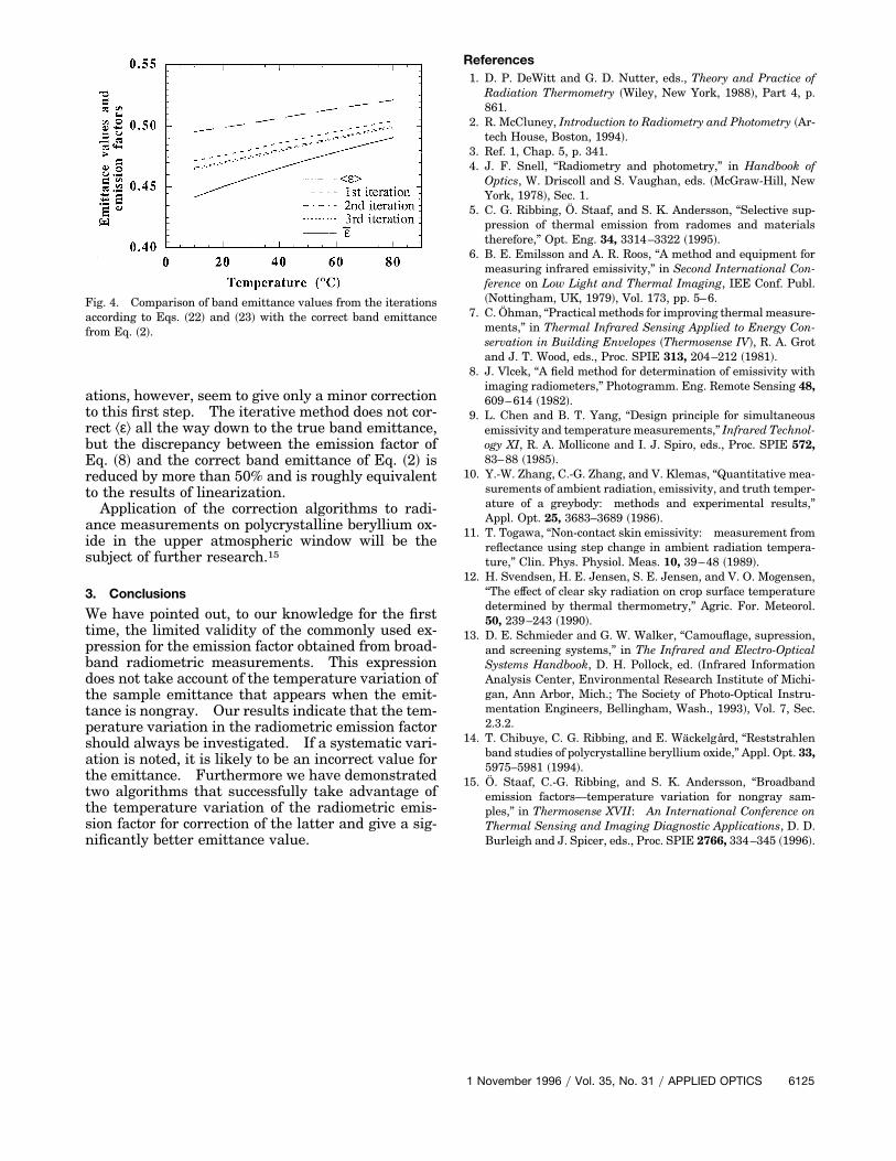
ations, however, seem to give only a minor correctionto this first step. The iterative method does not cor-rect ^ε& all the way down to the true band emittance,but the discrepancy between the emission factor ofEq. ~8! and the correct band emittance of Eq. ~2! isreduced by more than 50% and is roughly equivalentto the results of linearization.Application of the correction algorithms to radi-

ance measurements on polycrystalline beryllium ox-ide in the upper atmospheric window will be thesubject of further research.15

3. Conclusions

We have pointed out, to our knowledge for the firsttime, the limited validity of the commonly used ex-pression for the emission factor obtained from broad-band radiometric measurements. This expressiondoes not take account of the temperature variation ofthe sample emittance that appears when the emit-tance is nongray. Our results indicate that the tem-perature variation in the radiometric emission factorshould always be investigated. If a systematic vari-ation is noted, it is likely to be an incorrect value forthe emittance. Furthermore we have demonstratedtwo algorithms that successfully take advantage ofthe temperature variation of the radiometric emis-sion factor for correction of the latter and give a sig-nificantly better emittance value.

Fig. 4. Comparison of band emittance values from the iterationsaccording to Eqs. ~22! and ~23! with the correct band emittancefrom Eq. ~2!.

References1. D. P. DeWitt and G. D. Nutter, eds., Theory and Practice of

Radiation Thermometry ~Wiley, New York, 1988!, Part 4, p.861.

2. R. McCluney, Introduction to Radiometry and Photometry ~Ar-tech House, Boston, 1994!.

3. Ref. 1, Chap. 5, p. 341.4. J. F. Snell, “Radiometry and photometry,” in Handbook of

Optics, W. Driscoll and S. Vaughan, eds. ~McGraw-Hill, NewYork, 1978!, Sec. 1.

5. C. G. Ribbing, O. Staaf, and S. K. Andersson, “Selective sup-pression of thermal emission from radomes and materialstherefore,” Opt. Eng. 34, 3314–3322 ~1995!.

6. B. E. Emilsson and A. R. Roos, “A method and equipment formeasuring infrared emissivity,” in Second International Con-ference on Low Light and Thermal Imaging, IEE Conf. Publ.~Nottingham, UK, 1979!, Vol. 173, pp. 5–6.

7. C. Ohman, “Practical methods for improving thermalmeasure-ments,” in Thermal Infrared Sensing Applied to Energy Con-servation in Building Envelopes ~Thermosense IV!, R. A. Grotand J. T. Wood, eds., Proc. SPIE 313, 204–212 ~1981!.

8. J. Vlcek, “A field method for determination of emissivity withimaging radiometers,” Photogramm. Eng. Remote Sensing 48,609–614 ~1982!.

9. L. Chen and B. T. Yang, “Design principle for simultaneousemissivity and temperaturemeasurements,” Infrared Technol-ogy XI, R. A. Mollicone and I. J. Spiro, eds., Proc. SPIE 572,83–88 ~1985!.

10. Y.-W. Zhang, C.-G. Zhang, and V. Klemas, “Quantitative mea-surements of ambient radiation, emissivity, and truth temper-ature of a greybody: methods and experimental results,”Appl. Opt. 25, 3683–3689 ~1986!.

11. T. Togawa, “Non-contact skin emissivity: measurement fromreflectance using step change in ambient radiation tempera-ture,” Clin. Phys. Physiol. Meas. 10, 39–48 ~1989!.

12. H. Svendsen, H. E. Jensen, S. E. Jensen, and V. O. Mogensen,“The effect of clear sky radiation on crop surface temperaturedetermined by thermal thermometry,” Agric. For. Meteorol.50, 239–243 ~1990!.

13. D. E. Schmieder and G. W. Walker, “Camouflage, supression,and screening systems,” in The Infrared and Electro-OpticalSystems Handbook, D. H. Pollock, ed. ~Infrared InformationAnalysis Center, Environmental Research Institute of Michi-gan, Ann Arbor, Mich.; The Society of Photo-Optical Instru-mentation Engineers, Bellingham, Wash., 1993!, Vol. 7, Sec.2.3.2.

14. T. Chibuye, C. G. Ribbing, and E. Wackelgård, “Reststrahlenband studies of polycrystalline beryllium oxide,” Appl. Opt. 33,5975–5981 ~1994!.

15. O. Staaf, C.-G. Ribbing, and S. K. Andersson, “Broadbandemission factors—temperature variation for nongray sam-ples,” in Thermosense XVII: An International Conference onThermal Sensing and Imaging Diagnostic Applications, D. D.Burleigh and J. Spicer, eds., Proc. SPIE 2766, 334–345 ~1996!.

1 November 1996 y Vol. 35, No. 31 y APPLIED OPTICS 6125