Temperature correction coefficients of electrical ... · PDF fileWorking Report 2001-15...
45
Working Report 2001-15 Temperature correction coefficients of electrical conductivity and of density measurements for saline groundwater Mia Mäntynen June 2001 POSIVA OY Töölönkatu 4, FIN-00100 HELSINKI, FINLAND Tel. +358-9-2280 30 Fax +358-9-2280 3719
-
Upload
truongxuyen -
Category
Documents
-
view
218 -
download
2
Transcript of Temperature correction coefficients of electrical ... · PDF fileWorking Report 2001-15...

Working Report 2001-15
Temperature correction coefficients of electrical conductivity and of density
measurements for saline groundwater
Mia Mäntynen
June 2001
POSIVA OY
Töölönkatu 4, FIN-00100 HELSINKI, FINLAND
Tel. +358-9-2280 30
Fax +358-9-2280 3719

Working Report 2001-15
Temperature correction coefficients of electrical conductivity and of density measurements for saline groundwater
Mia Mäntynen
June 2001

TEKIJÄORGANISAATIO:
TEKIJÄ:
TARKASTANUT:
HYVÄKSYNYT:
Posiva Oy Töölönkatu 4 00100 HELSINKI
Working Report 2001-15
Temperature correction coefficients of electrical conductivity and of density measurements for saline groundwater
Mia Mäntyneo Posiva Oy
'/ne'-- JY/{i;~
Margit Snellman Posiva Oy. . .L ~~+~&------
Juhani Vira Posiva Oy
L \ \
-------
L ____________________________________________________________________________ _
Working Report 2001-15
Temperature correction coefficients of electrical conductivity and of density measurements for saline groundwater
Mia Mäntynen
Posiva Oy
June 2001
Working Reports contain information on work in progress
or pending completion.
TEMPERATURE CORRECTION COEFFICIENTS OF ELECTRICAL CONDUCTIVITY AND DENSITY MEASUREMENTS FOR SALINE GROUNDWATERS
ABSTRACT
Electrical conductivity (EC) is strongly dependent on the temperature of the samples. The EC results are usually established at 25 °C, which is the commonly used reference temperature. Measuring results at different temperatures can be corrected to 25 oc by using temperature correction coefficients that depend on the nature of the samples. Measurements at six different temperatures and eleven concentrations are made to give the basis for the temperature correction coefficients in saline waters.
The temperature correction coefficient of the EC is established by measuring the EC of the solution at least in the two different stable temperatures. Measurements of the samples from the Olkiluoto and Hästholmen, of the OLSO and Allard reference waters and of some artificial samples were made. Artificial samples consisted of N aCl and CaCh salts and the concentration of the solutions were between 0-1 00 g/1. The most important aim of this work was to establish several calibration points for mathematic modelling. The temperature correction coefficients for electrical conductivity can be calculated by using the mathematic model. Preparation of solutions for the measurements and the way the measurements were done are presented in this report. Based on results of this study it can be noticed that temperature correction coefficients are decreasing when the salinity of the solution increases.
The density of the solutions is increasing while the concentration of the solution increases. Density is dependent on the temperature of the solution, too. The temperature correction coefficients of densities were calculated in this study as well. The densities of the solutions were measured by two different methods and the results were compared to the values from the literature. Samples were artificial NaCl- and CaCh-solutions. Calculated temperature coefficients were small. They affected only to the fourth decimal of the measuring result. The use of the temperature coefficients should be avoided in this case because all the density measurements are usually done in laboratory where the samples can be stabilised to known temperature. The densities of the solutions were measured in two ways: by using automatic Anton Paar DMA 35N density meter and by the weighing method in the laboratory of the F ortum in V antaa. The results were almost the same and they differed from the literature values only when the TDS (Total Dissolved Solids) was >50 g/1.
Keywords: Electrical conductivity, density, groundwater, temperature correction coefficient, TDS
SÄHKÖNJOHTAVUUS- JA TIHEYSMITTAUSTEN LÄMPÖTILAKORJAUSKERTOIMET SUOLAISILLE POHJA VESILLE
TIIVISTELMÄ
Liuoksen sähkönjohtavuus riippuu voimakkaasti liuoksen lämpötilasta. Jotta eri lämpötiloissa mitattuja sähkönjohtavuusarvoja voidaan verrata toisiinsa, ne on korjattava yleisesti käytettyyn vertailulämpötilaan (T = 25 °C). Eri lämpötiloissa mitatut sähkönjohtavuudet voidaan korjata vertailulämpötilaan lämpötilakorjauskertoimia käyttämällä. Lämpötilakorjauskertoimien suuruus riippuu näytteen ominaisuuksista. Yhdelletoista erilaisen konsentraation omaavalle suolaliuokselle kuudessa eri lämpötilassa suoritetut sähkönjohtavuusmittaukset luovat perustan suolaisten pohjavesien lämpötilakorj aukselle.
Sähkönjohtavuuden lämpötilakorjauskertoimien määritys tapahtuu mittaamalla liuoksen lämpötila vähintään kahdessa termostoidussa lämpötilassa. Näytteinä oli Olkiluodon ja Hästholmenin kairanreikien pohjavesiä, OLSO- ja Allard-referenssivedet sekä joukko keinotekoisia suolaliuoksia, joissa suolaina olivat NaCl ja CaCb ja joiden konsentraatio vaihteli välillä 0-100 g/1. Tämän työn tärkein tarkoitus oli tuottaa mallintajien käyttöön kalibrointipistejoukko, jota käyttäen sähkönjohtavuuden lämpötilakorjaukselle voidaan määrittää laskennallinen malli. Tässä raportissa esitellään yksityiskohtaisesti mittauksissa käytettyjen liuosten valmistus sekä mittausten suoritustapa. Tämän työn tulosten perusteella voidaan osoittaa, että lämpötilakorjauskertoimet pienenevät suolapitoisuuden kasvaessa.
Liuoksen tiheys kasvaa suolapitoisuuden kasvaessa. Tiheyden määritys on myös riippuvainen liuoksen lämpötilasta mittaushetkellä. Tässä työssä määritettiin myös tiheyksille lämpötilakorjauskertoimet sekä verrattiin kahdella eri mittausmenetelmällä saatuja tuloksia kirjallisuusarvoihin. Näytteinä määrityksissä käytettiin keinotekoisia NaCl- ja CaCb-suolaliuoksia. Määritetyt lämpötilakorjauskertoimet olivat hyvin pieniä. Niiden vaikutus ulottui ainoastaan mittaustuloksen neljänteen desimaaliin. Korjauskertaimien käyttöä tulee välttää, sillä mittaukset suoritetaan yleensä laboratoriossa, jossa näytteiden termostointi referenssilämpötilaan on mahdollista. Tiheyden määrityksissä käytettiin kahta eri menetelmää: automaattista Anton Paar DMA 35N tiheysmittaria ja Fortum Power and Heat Oy:n käyttämää punnitukseen perustuvaa menetelmää. Molemmilla menetelmillä tulokset poikkesivat kirjallisuusarvoista vasta, kun liuoksen TDS (Total Dissolved Solids) oli> 50 g/1.
Avainsanat: Sähkönjohtavuus, tiheys, pohjavesi, lämpötilakorjauskerroin, TDS
TABLE OF CONTENTS
Abstract
Tiivistel mä
1 INTRODUCTION 3
2 DEFINITION OF THE ELECTRICAL CONDUCTIVITY . . . . . . . . . . . . . . . . . . . . . . 4
3 DEFINITION OF DENSITY OF WATER SAMPLES . . . . . . . . . . . . . . . . . . . . . . . . 8
4 EXPERIMENTAL CONDITIONS . . . . . . . . . . . . . . . . . . . . . . . . . . . . . . . . . . . . . . . . . . 9
5 DEFINITION OF TEMPERATURE CORRECTION COEFFICIENTS . . . . . . . . . 13
5.1 Oireet definition of the temperature correction coefficient from the conductivity values measured at temperatures 5 and 25 oc . . . . . . . . . . . 1 3
5.2 Effect of sulfate on the temperature correction coefficient of the NaCI solution . . . . . . . . . . . . . . . . . . . . . . . . . . . . . . . . . . . . . . . . . . . . . . . . . . . . . 1 9
6 DENSITY MEASUREMENTS . . . . . . . . . . . . . . . . . . . . . . . . . . . . . . . . . . . . . . . . . . . . . 21
7 DISCUSSION . . . . . . . . . . . . . . . . . . . . . . . . . . . . . . . . . . . . . . . . . . . . . . . . . . . . . . . . . . 23
7.1 Temperature correction coefficients of the electrical conductivity measurements . . . . . . . . . . . . . . . . . . . . . . . . . . . . . . . . . . . . . . . . . . . . . . . . . . . . 23
7.2 Density measurements of the saline waters . . . . . . . . . . . . . . . . . . . . . . . . . 23
8 SUMMARY . . . . . . . . . . . . . . . . . . . . . . . . . . . . . . . . . . . . . . . . . . . . . . . . . . . . . . . . . . . . . 26
9 REFERENCES . . . . . . . . . . . . . . . . . . . . . . . . . . . . . . . . . . . . . . . . . . . . . . . . . . . . . . . . . 28
10 APPENDICES . . . . . . . . . . . . . . . . . . . . . . . . . . . . . . . . . . . . . . . . . . . . . . . . . . . . . . . . . . 30
APPENDIX 1: TEMPERATURE CORRECTION COEFFICIENTS OF THE NATURAL WATERS FROM THE SFS-STANDARD . . . . . . . . . . . . . . . . . 31
APPENDIX 2: DENSITY OF WATER FROM 0 TO 40 OC . . . . . . . . . . . . . . . . . . . . . . . . . 32
APPENDIX 3: DENSITIES OF NACL SOLUTIONS . . . . . . . . . . . . . . . . . . . . . . . . . . . . . . 33
APPENDIX 4: DENSITIES OF CACL2 SOLUTIONS . . . . . . . . . . . . . . . . . . . . . . . . . . . . . . 34
APPENDIX 5: TEMPERATURE COEFFICIENT OF THE DENSITY MEASUREMENTS FOR THE SAMPLES WITH A TDS = 5 g/1 CALCULATED BY USING THE POLYNOMIAL . . . . . . . . . . . . . . . . . . . . . 35
APPENDIX 6: TEMPERATURE COEFFICIENT OF THE DENSITY MEASUREMENTS FOR THE SAMPLES WITH A TDS = 10 g/1 CALCULATED BY USING THE POLYNOMIAL . . . . . . . . . . . . . . . . . . . . . 36

2
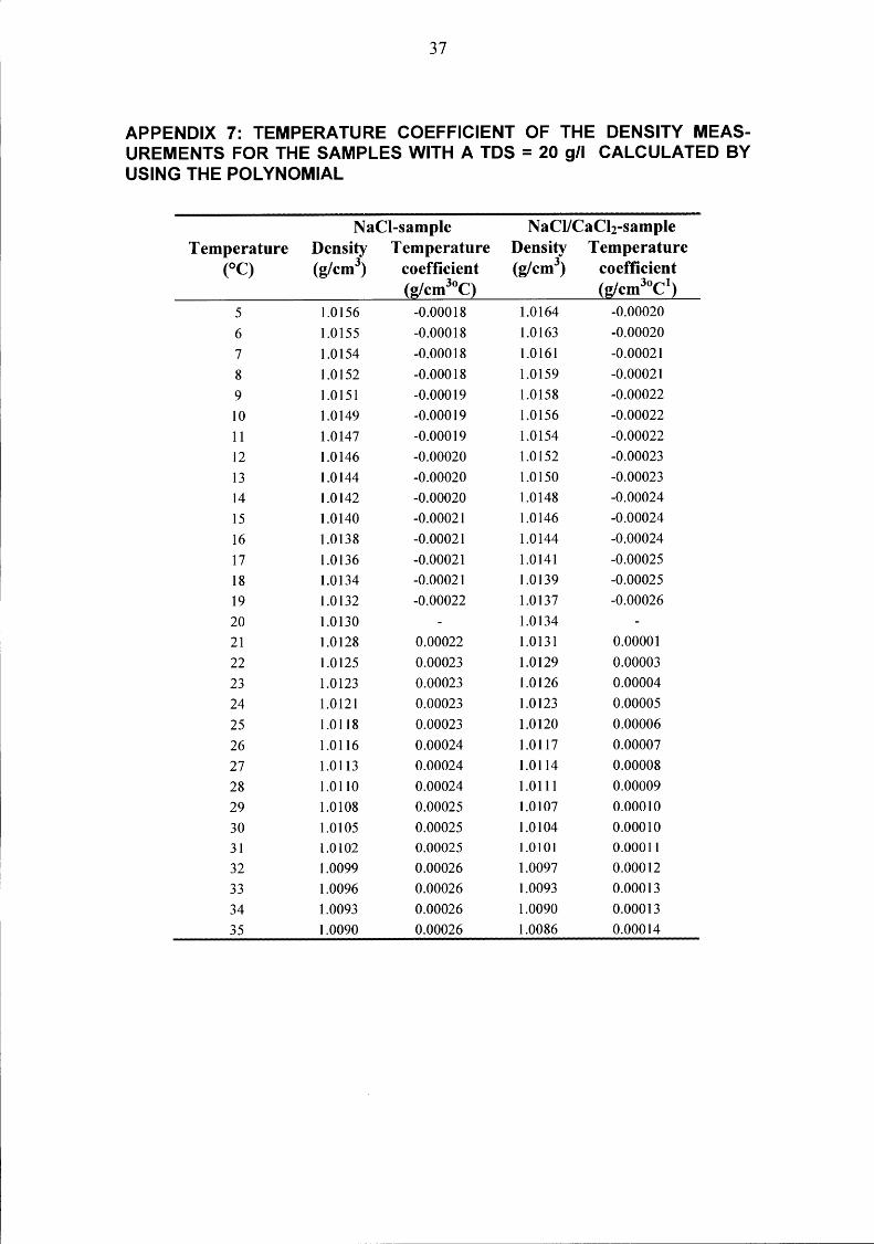
APPENDIX 7: TEMPERATURE COEFFICIENT OF THE DENSITY MEASUREMENTS FOR THE SAMPLES WITH A TDS = 20 g/1 CALCULATED BY USING THE POL YNOMIAL . . . . . . . . . . . . . . . . . . . . . 3 7
APPENDIX 8: TEMPERATURE COEFFICIENT OF THE DENSITY MEASUREMENTS FOR THE SAMPLES WITH A TDS = 50 g/1 CALCULATED BY USING THE POLYNOMIAL . . . . . . . . . . . . . . . . . . . . . 38
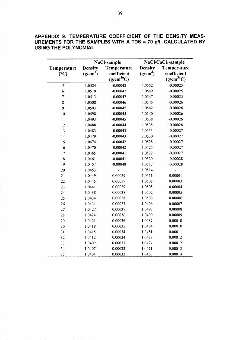
APPENDIX 9: TEMPERATURE COEFFICIENT OF THE DENSITY MEASUREMENTS FOR THE SAMPLES WITH A TDS = 70 g/1 CALCULATED BY USING THE POLYNOMIAL . . . . . . . . . . . . . . . . . . . . . 39
APPENDIX 10: TEMPERATURE COEFFICIENT OF THE DENSITY MEASUREMENTS FOR THE SAMPLES WITH A TDS = 100 g/1 CALCULATED BY USING THE POLYNOMIAL . . . . . . . . . . . . . . . . . . . . . 40

3
1. INTRODUCTION
The difference flow method (DIFF) is used in Posiva's site investigations for hydraulic characterization of electrical conductivities of eaters in fractures and fracture zones. The DIFF -equipment includes a 4-electrode conductivity measuring system. The electrical conductivity is measured in-situ in the borehole at ambient temperature. Because the electrical conductivity is strongly dependent on the temperature of the sample the results are usually transformed to correspond 25 °C. Measuring results from the different temperatures can he corrected to 25 oc by using temperature correction coefficients, which depend on the nature of the samples.
As known as a fact the density of the solution increases with increasing concentration. The densities of different sait solutions are measured by using two different methods in this study. Density of the solution is also dependent on it's temperature. Temperature correction coefficient of the density measurements is measured for samples, which have different TDS values.
Groundwater samples from Olkiluoto and Hästholmen were ehosen for the electrical conductivity measurements and temperature coefficient calculations. Beside these also saline and fresh reference waters (Vuorinen & Snellman 1998) and artificial samples were measured. Artificial samples were made by dissolving known amounts of NaCl and CaCh salts into theultrapure water. The electrical conductivities of all these samples were measured at two stable temperatures and the temperature coefficients were calculated. Electrical conductivity of additional artificial samples was measured at several different temperatures and the temperature coefficients were calculated. Calculated temperature coefficients were compared with the values from the literature. The effect of sulphate on the temperature correction coefficient ofthe NaCl-solution was also studied.
12 samples were prepared for the density measurements. Six of these were made from pure NaCl and six were made from a mixture of 50% of NaCl and 50 % of CaCh. The densities of the solutions were measured at 5 different temperatures and the temperature correction coefficients were calculated. Densities at 20 oc were measured with two different methods. Results from the different methods are compared with each other and with the values from the literature.

4
2. DEFINITION OF THE ELECTRICAL CONDUCTIVITY
Electrical conductivity is a measure of the ability of a solution to carry an electric current. Solutions of electrolytes conduct an electric current by migration of ions under the influence of an electric field. The current obeys Ohm' s law:
1= E R
where 1 = electric current (A),
E = electromotive force (V),
R = resistance (Ohm).
(1)
The measurement of a solution's resistance R, in a conductivity cell, is used to determine the conductivity of a solution. The resistance of a solution is proportional to the distance between the electrodes d and inversely proportional to the effective crosssectional area, A (Jamel et al. 2000).
d R=p
A
where R = resistance (Ohm),
A = effective cross-sectional area (m2),
p = resistivity, constant for given solution (Ohm·m),
d = distance between electrodes (m).
(2)
Electrical conductivity K is defined as the reciprocal of the resistance R. It is expressed in Siemens per metre usually at a reference temperature of 25 oc (Jamel et al. 2000).
1 d K=-=-
p RA (3)
where K = electrical conductivity (S/m),
5
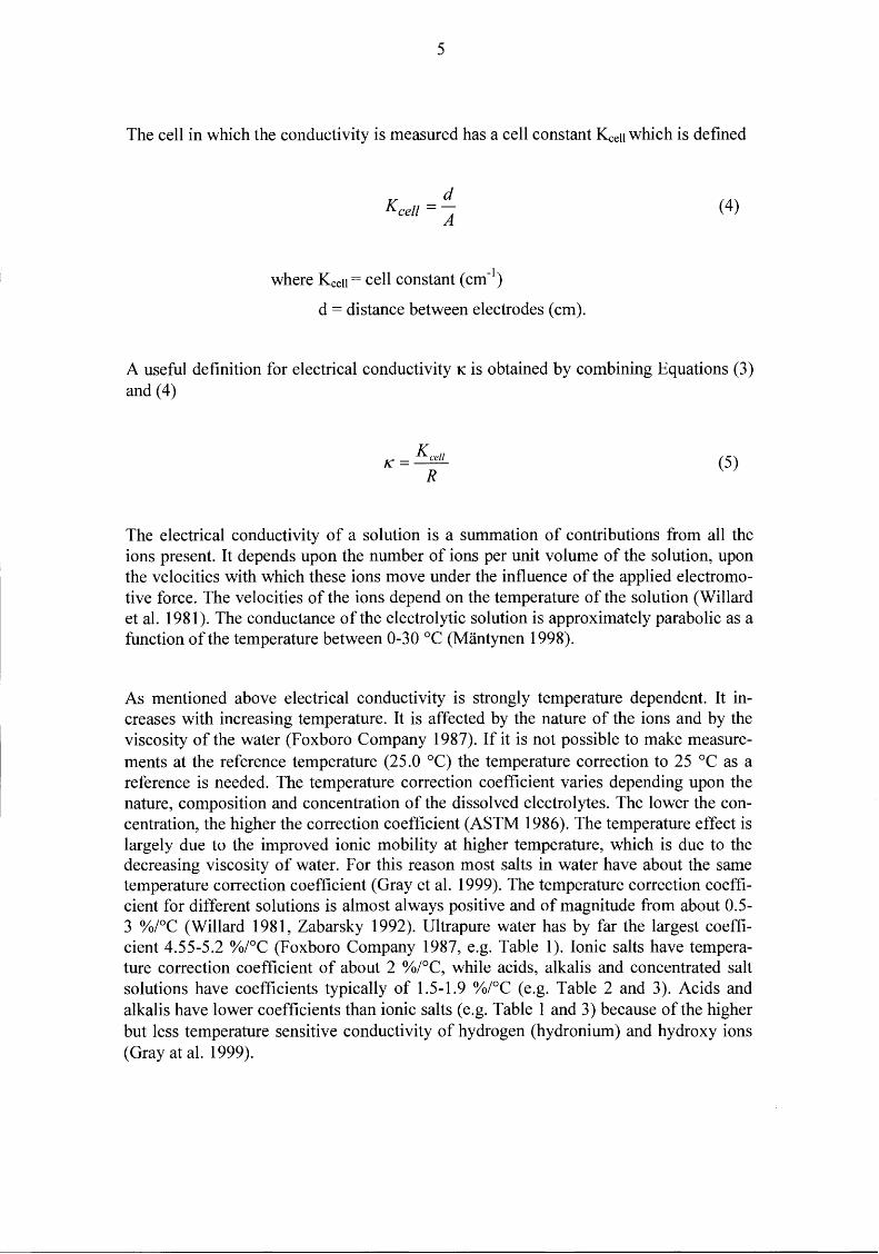
The cell in which the conductivity is measured has a cell constant Kcen which is defined
d Kcell = A
where Kcell = cell constant (cm -I)
d = distance between electrodes (cm).
(4)
A useful definition for electrical conductivity K is obtained by combining Equations (3) and (4)
(5)
The electrical conductivity of a solution is a summatien of contributions from all the ions present. It depends upon the number of ions per unit volume of the solution, upon the velocities with which these ions move under the influence of the applied electromotive force. The velocities of the ions depend on the temperature of the solution (Willard et al. 1981 ). The conductance of the electrolytic solution is approximately parabolic as a function ofthe temperature between 0-30 oc (Mäntynen 1998).
As mentioned above electrical conductivity is strongly temperature dependent. It increases with increasing temperature. It is affected by the nature of the ions and by the viscosity of the water (Foxboro Company 1987). If it is not possible to make measurements at the reference temperature (25.0 °C) the temperature correction to 25 oc as a reference is needed. The temperature correction coefficient varies depending upon the nature, composition and concentration of the dissolved electrolytes. The lower the concentration, the higher the correction coefficient (ASTM 1986). The temperature effect is largely due to the improved ionic mobility at higher temperature, which is due to the decreasing viscosity of water. For this reason most salts in water have about the same temperature correction coefficient (Gray et al. 1999). The temperature correction coefficient for different solutions is almost always positive and of magnitude from about 0.5-3 %/°C (Willard 1981, Zabarsky 1992). Ultrapure water has by far the largest coefficient 4.55-5.2 %/°C (Foxboro Company 1987, e.g. Table 1). Ionic salts have temperature correction coefficient of about 2 %!°C, while acids, alkalis and concentrated salt solutions have coefficients typically of 1.5-1.9 %/°C ( e.g. Table 2 and 3). Acids and alkalis have lower coefficients than ionic salts ( e.g. Table 1 and 3) because of the higher but less temperature sensitive conductivity of hydrogen (hydronium) and hydroxy ions (Gray at al. 1999).

6
Table 1. Common temperature correction coefficients for different solutions. (references: http://www.orionres.com/ionguide/english/ion24eng.html,
http ://www .eutechinst.com/techtips/tech-tips25 .htm)
Sample Temperature coefficient
(o/o/oC)
10% HCl 1.56 (1.32*)
10% KCl 1.88
5% H2S04 0.96
50% H2S04 1.93
98% H2S04 2.84
10% NaCl 2.14
Ultrapure water 4.55
5% NaOH 1.72
* Different values in different references.
Table 2. Average temperature correction coefficients of standard electrolyte solutions (reference: Radiometer Copenhagen: Operating lnstructions).
Temperature Range 1MKCI 0.1 M KCI 0.01 M KCI Saturated NaCI (oC) (o/ofOC) (
0/ofOC) (0/ofOC) (
0/ofOC)
15-25 1.735 1.863 1.882 1.981
15-25-35 1.730 1.906 1.937 2.041
(15-27)* (15-34)*
25-35 1.730 1.978 1.997 2.101
(25-27)* (25-34)*
* Exceptional temperature range, oc
Table 3. Temperature correction coefficients of electrical conductivity, when the con-centration ofthe salt is 0.01 g/mol (Forsythe 1956).
Salt Temp. Salt Temp. Salt Temp. Salt Temp.
Coeff. Coeff. Coeff. Coeff.
(0/ofOC) (o/o/oC) (
0/ofOC) (0/ofOC)
KCl 2.21 KI 2.19 Yz K2S04 2.23 Yz K2C03 2.49
NH4Cl 2.26 KN03 2.16 Yz Na2S04 2.40 Yz Na2C03 2.65
NaCl 2.38 NaN03 2.26 Yz LhS04 2.42 KOH 1.94
LiCl 2.32 AgN03 2.21 Yz Mg2S04 2.36 HCl 1.59
Yz BaCh 2.34 Yz Ba(N03)2 2.24 Yz ZnS04 2.34 HN03 1.62
Yz ZnCh 2.39 KC103 2.19 Yz CuS04 2.29 Yz H2S04 1.25
Yz MgCh 2.41 KC2H30 2 2.29 Yz H2S04 1.59

7
The temperature correction coefficient can be measured. lt requires a series of conductivity and temperature measurements on the sample over the required temperature range. Measured conductivity can be plotted against the temperature and compensation curve is drawn from this data. A 2-point compensation may be used with an exact match at two temperatures. Some error may exist at the intermediate temperatures (ASTM 1986, Foxboro Company 1987). The 2-point temperature coefficient can be calculated by the equation:
8 = _1_(KT- Kref J ·100 Kref T -Tref
where e = temperature correction coefficient (%/°C),
T = measuring temperature (°C),
KT = electrical conductivity of the sample at T (S/m, mS/m or f.tS/m),
Tref = Reference temperature 25 °C,
(3)
Kref = electrical conductivity ofthe sample at Tref (S/m, mS/m or f.tS/m).
It must be noticed that this temperature correction coefficient can be used only between Tand Tref·
Conversion to the electrical conductivity at 25 °C, can be made by using the equation (SFS-EN27888, 1994):
Kr K -------~-------
ref- 1 + (B /100)(T- Tref) (4)

8
3. DEFINITION OF DENSITY OF WATER SAMPLES
Density is defined as mass per unit volume and is calculated by dividing the mass of an ohjeet by its volume (Ranta et al. 1991).
m p=v
where p = density of the sample (g/cm3 or kg/m3),
m = mass of the sample (g or kg),
V = volume of the sample ( cm3 or m3).
(5)
Density is affected by the temperature. Densities of pure water at different temperatures are listed in Appendix 2. Influence of sample temperature is compensated using the temperature coefficient (gcm-3K-1
). Temperature coefficients for most aqueous samples at 20 oc are between 3·10-4-5·10-4 g/cm3K. The temperature coefficient, k can be calculated according to theformula (Herbst 1998):
where
(6)
p1 = density at temperature T1 ( [ pi] = g/cm3 or kg/m3, [TI] = oc or
K).
P2 = density at temperature T2 ( [ P2l = g/cm3 or kg/m3, [T2] = oc or
K).
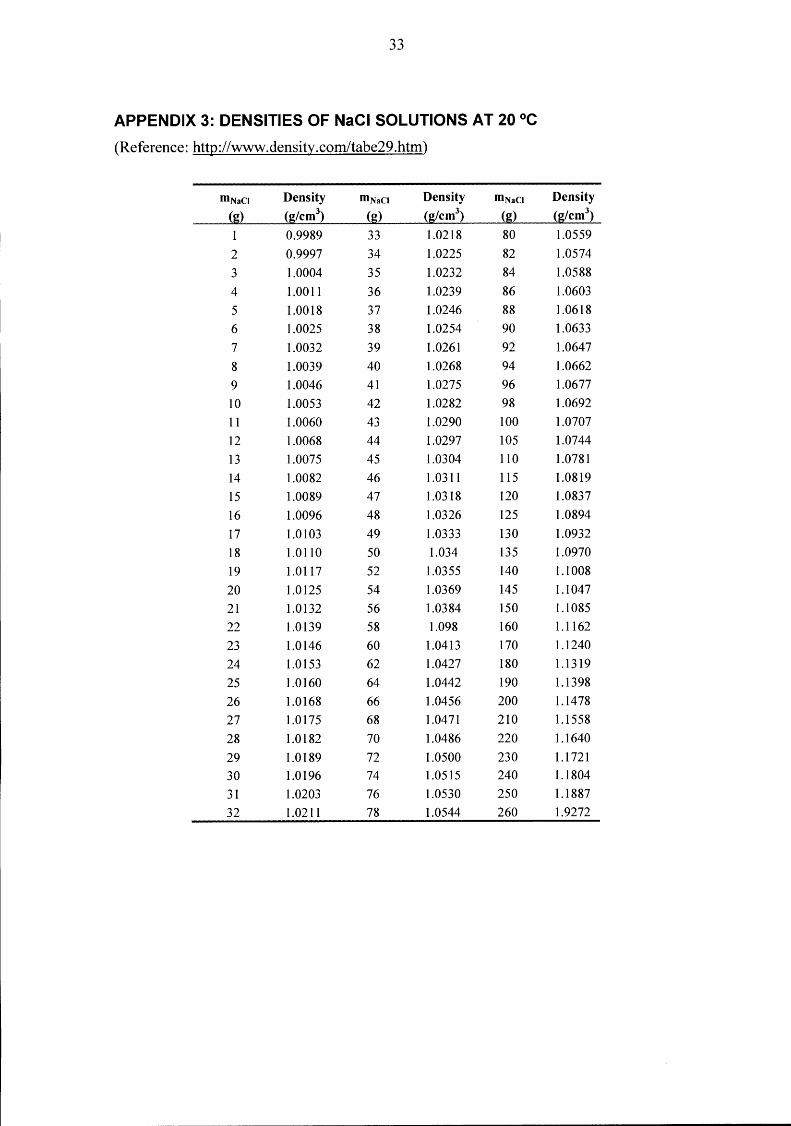
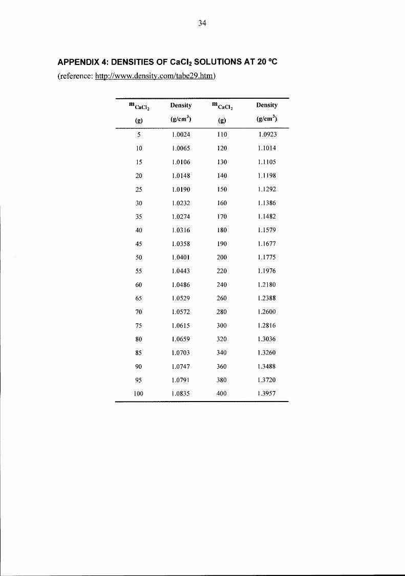
As evident density also increases as the concentration of the solution increases. As an example, the density of NaCl and CaCh solutions at different concentrations, is shown in Appendices 3 and 4.
(http://www.density.com/tabe29.htm, http://www.density.com/calcium2.htm)

9
4. EXPERIMENT AL CONDITIONS
Measurements to determine temperature correction coefficients of the electrical conductivity for saline groundwater were done in July 1999 and May 2000. Results of the measurements done in July 1999 have been reported in Mäntynen 2000 (in Finnish). They are presented briefly together with the new measuring results in this report, too.
In July 1999 the temperature correction coefficients were determined for six real groundwater samples, for saline and fresh reference waters and for eight artificial samples. Groundwater samples were ehosen so that they represent different salinities. They were frozen spare samples both from Olkiluoto and Hästholmen. The saline (OL-SO) and the fresh (Allard) reference waters were made according to the instructions (Vuorinen & Snellman 1998). The artificial samples consists of 50 % NaCl and 50 % CaCh·2H20 salts. The effect of the water of crystallization to the mass of the CaCh·2H20 has not been considered here. Both salts were weighed with the Mettler AE 240 balance to the same volumetric flask of 250 ± 0.15 ml. The accuracy of the balance is ± 0.02 g. Salts were dissolved to a small amount of ultrapure water and the flask was filled with ultrapure water. The TDS (Total Dissolved Solids) value of the artificial samples varies between 10 - 56 g/1. The relative error of the TDS value is depending on the error of the weights and the error of the volume of the volumetric flask. The relative error (%) for the TDS was calculated by using equation (7).
where V = volume of the volumetric flask (ml),
m = weight of the salts (g)
(7)
10
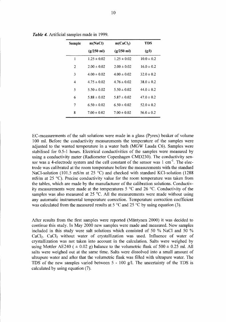
Table 4. Artificial samples made in 1999.
Sample m(NaCI) m(CaCh) TDS
(g/250 ml) (g/250 ml) (g/1)
1.25 ± 0.02 1.25 ± 0.02 10.0 ± 0.2
2 2.00 ± 0.02 2.00 ± 0.02 16.0 ± 0.2
3 4.00 ± 0.02 4.00 ± 0.02 32.0 ± 0.2
4 4.75 ± 0.02 4.76 ± 0.02 38.0 ± 0.2
5 5.50 ± 0.02 5.50 ± 0.02 44.0 ± 0.2
6 5.88 ± 0.02 5.87 ± 0.02 47.0 ± 0.2
7 6.50 ± 0.02 6.50 ± 0.02 52.0 ± 0.2
8 7.00 ± 0.02 7.00 ± 0.02 56.0 ± 0.2
EC-measurements of the salt solutions were made in a glass (Pyrex) beaker of volume 100 ml. Before the conductivity measurements the temperature of the samples were adjusted to the wanted temperature in a water bath (MGW Lauda C6). Samples were stabilised for 0.5-1 hours. Electrical conductivities of the samples were measured by using a conductivity meter (Radiometer Copenhagen CMD230). The conductivity sensor was a 4-electrode system and the cell constant of the sensor was 1 cm-1
. The electrode was calibrated at the room temperature before the measurements with thestandard NaCl-solution (101.5 mS/m at 25 °C) and checked with standard KCl-solution (1288 mS/m at 25 °C). Precise conductivity value for the room temperature was taken from the tables, which are made by the manufacturer of the calibration solutions. Conductivity measurements were made at the temperatures 5 oc and 26 °C. Conductivity of the samples was also measured at 25 °C. All the measurements were made without using any automatic instrumental temperature correction. Temperature correction coefficient was calculated from the measured results at 5 oc and 25 oc by using equation (3).
After results from the first samples were reported (Mäntynen 2000) it was decided to continue this study. In May 2000 new samples were made and measured. New samples included in this study were salt solutions which consisted of 50 % NaCl and 50 % CaCh. CaCh without water of crystallization was used. Influence of water of crystallization was not taken into account in the calculation. Salts were weighed by using Mettler AE240 ( ± 0.02 g) balance to the volumetric flask of 500 ± 0.25 ml. All salts were weighed out at the same time. Salts were dissolved into a small amount of ultrapure water and after that the volumetric flask was filled with ultrapure water. The TDS of the new samples varied between 5 - 100 g/1. The uncertainty of the TDS is calculated by using equation (7).

11
Table 5. Artificial samples made in 2000.
Sample m(NaCI) m(CaCh) TDS
(g/500 ml) (g/500 ml) (g/1)
1.2511 ± 0.0200 1.2504 ± 0.0200 5.0 ± 0.1
2 2.5018 ± 0.0200 2.4994 ± 0.0200 10.0 ± 0.1
3 3.7523 ± 0.0200 3.7456 ± 0.0200 15.0 ± 0.1
4 5.0020 ± 0.0200 5.0010 ± 0.0200 20.0 ± 0.1
5 6.2507 ± 0.0200 6.2480 ± 0.0200 25.0 ± 0.1
6 7.5090 ± 0.0200 7.4989 ± 0.0200 30.0 ± 0.1
7 8.7522 ± 0.0200 8.7529 ± 0.0200 35.0±0.1
8 10.0039 ± 0.0200 9.9948 ± 0.0200 40.0 ± 0.1
9 12.5000 ± 0.0200 12.4950 ± 0.0200 50.0 ± 0.1
10 17.5017 ± 0.0200 17.4977 ± 0.0200 70.0 ± 0.1
11 25.0081 ± 0.0200 24.9935 ± 0.0200 100.0 ± 0.1
Samples were stabilised to the temperatures 5, 10, 15, 20, 25 and 30 oc in the thermostatically controlled water bath and conductivity measurements were made without using any automatic temperature correction. The stabilisation procedure was started from 5 oc and ended at 30 °C. The instrument and the calibration procedure was the same as 1999 (Mäntynen 2000). Temperature coefficients were calculated from the measured conductivity results at 5 oc and 25 oc by using equation (3 ).
The effect of sulphate on temperature correction coefficient of the NaCl solution was also examined in May 2000. Two test solutions were made, one pure NaCl solution (CNaCI = 5 g/1) and the other a NaCl/Na2S04 solution (CNaCI = 5 g/1 and Na2S04 was weighed so that Cso4= 1 g/1). Solutions and measurements were made as above. The electrical conductivity of the solutions was measured without automatic temperature correction at the stabilised temperatures: 5, 10, 15, 20, 25, and 30 °C. The temperature coefficients were calculated from the measured results, either by calculating from the conductivity measuring results at 5 oc and 25 °C by using equation (3) or by plotting EC results against the temperature. The second degree fit-function was calculated from the established points. New conductivity values were calculated for every temperature between 0-30 oc by using fit-functions. After that the temperature correction coefficients for different temperatures were calculated by using calcu1ated conductivity values.
12 samples were prepared for the density measurements. The TDS values of the samples were 5, 10, 20, 50, 70 and 100 g/1. Six samples contained 50 % NaCl and 50 % CaCh (without crystal waters). The other six samples were pure NaCl solutions. The salts were weighed with the Mettler AE240 (± 0.02 g) and Mettler Toledo PB5001 (± 0.1 g) balances to a volumetric flask (500 ± 0.25 ml). Salts were dissolved into small amount of ultrapure water and after that the volumetric flask was filled with ultrapure water. The uncertainty ofthe TDS is calculated by using equation (7).

12
Table 6. Artificial samples made for the density measurements in 2000.
Sample m(NaCI) m(CaCI2) TDS
(g/500 ml) (g/500 ml) (g/1)
Series 1: 2.5027 ± 0.0200 5.0 ± 0.1
2 5.0055 ± 0.0200 10.0 ± 0.1
3 10.0016 ± 0.0200 20.0 ± 0.1
4 25.0027 ± 0.0200 50.0 ± 0.1
5 35.0 ± 0.1 70.0 ± 0.2
6 50.0 ± 0.1 100.0 ± 0.2
Series 2:
1 1.2515 ± 0.0200 1.2515 ± 0.0200 5.0 ± 0.1
2 2.5020 ± 0.0200 2.4999 ± 0.0200 10.0±0.1
3 5.0000 ± 0.0200 5.0000 ± 0.0200 20.0 ± 0.1
4 12.5 ± 0.1 12.5 ± 0.1 50.0 ± 0.4
5 17.5 ± 0.1 17.5 ± 0.1 70.0 ± 0.4
6 25.0 ± 0.1 25.0 ± 0.1 100.0 ± 0.4
Densities were measured by using an automatic density meter (at Fortum Power and Heat Oy (FPH), Loviisa Power Plant) and manually by weighing (FPH, Vantaa). In Loviisathe measurements were made at the stable temperatures: 16.5 or 17.5, 20, 25, 30 and 35 oc by using the automatic density meter Anton Paar DMA35N. Automatic density meter needs only couple of millilitres of sample for one measurement. The sample is injected direct to the meter from the sample vessel. The main advantage of the automatic density meter is it' s quickness. It takes less than a minute to measure density of one sample. The temperature coefficient was calculated from the measured results by using equation ( 6). In Vantaa the measurements were done manually by weighing at 20 °C according to instructions by the manufacturer (Mettler 210250).

13
5. DETERMINATION OF TEMPERATURE CORRECTION COEFFICIENTS
5.1. Oireet determination of the temperature correction coefficient from the conductivity values measured at temperatures 5 and 25 °C
The results from the measurements made in July 1999 and May 2000 and calculated temperature coefficients are presented. The temperature correction coefficients are applicable for the temperature area from 5 to 25 °C. Calculations were made by using equation (3). Temperature correction coefficients are calculated here just for an example. From calculated values it can be seen how much they deviate from commonly known temperature correction coefficients. These coefficients must not be used for any temperature correction calculations for EC-measurements. The relative error of the EC for the real samples is depending on the accuracy of the electrical conductivity meter (Table 7) and on the accuracy ofthe temperature bath (± 0.1 °C).
Table 7. The accuracy ofthe Radiometer Copenhagen CMD230 conductivity meter.
Conductance Accuracy Measuring range frequency
(Hz)
0.001- 4.000 f.!S ± 0.5 % of reading ± 3 lsd 1) 94
0.01- 40.00 f.!S 94
0.1- 400.0 f.!S 375
0.001-4.000 mS ± 0.2 % of reading ± 3 lsd 1) 2930
0.01- 40.00 mS 23400
0.1- 400.0 mS 46900
1-2000 mS ± 1 % of reading ±3 on lsd 1) 46900
1) least significant digit
The relative error of the electrical conductivity results presented in Table 8 has been calculated by using equation (8).
(8)
The uncertainty of the temperature coefficient is calculated by using equation 9.

fl.(}
{}
14
(9)
The uncertainty ofthe temperature coefficient is expanded to the 95% confidence level by multiplying fl.8 by factor 2.
Table 8. Electrical conductivity and calculated temperature coefficients for the groundwater samples and for the OL-SO and Allard reference waters measured in July 1999.
Groundwater samples
OL-KR4 OL-KKR8/P1
OL-KR5/T7
HH-KR4
HH-KR3
HH-KR5
Reference waters OL-SO 1/99
Allard 4/98
* Measuring error.
Electrical
Conductivity
Kzsoc (S/m)
9.48 ± 0.04 0.322 ± 0.001
0.247 ± 0.001
4.78 ± 0.02
1.299 ± 0.006
0.347 ± 0.002
3.84 ±0.02
0.0438 ± 0.0002
Electrical Temperature
Conductivity Coefticient
Ksoc (S/m) ( 0/o 1 °C)
6.05 ± 0.12 1.81 ± 0.07 0.196 ± 0.004 1.95 ± 0.08
0.148 ± 0.003 2.00 ± 0.08*
2.99 ± 0.06 1.88 ± 0.08
0.794 ± 0.016 1.94 ± 0.08
0.238 ± 0.005 1.88 ± 0.08
2.38 ±0.05 1.90 ± 0.08
0.0271 ±0.0005 1.91 ± 0.07
The relative error of the EC measurements for the artificial samples (Table 9) is depending on the error of the solutions concentration and the error of the conductivity meter. It is also depending on the accuracy of the temperature of the water bath (± 0.1 °C). The error is calculated by using equation 10.
MC = (!:J.TDS) 2 +(!:J.Meter) 2 +(!:J.T) 2
EC TDS Meter T (10)
The uncertainty of the temperature coefficient is calculated by using equation 9.
15
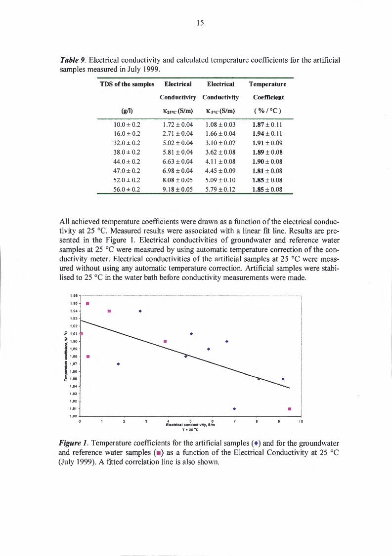
Table 9. Electrical conductivity and calculated temperature coefficients for the artificia1 samples measured in July 1999.
TDS of the samples Electrical Electrical Temperature
Conductivity Conductivity Coefficient
(g/1) Kzsoc (S/m) Ksoc(S/m) (% /°C)
10.0 ± 0.2 1.72 ± 0.04 1.08 ± 0.03 1.87 ± 0.11 16.0 ± 0.2 2.71 ± 0.04 1.66 ± 0.04 1.94 ± 0.11
32.0± 0.2 5.02 ± 0.04 3.10 ± 0.07 1.91 ± 0.09
38.0± 0.2 5.81 ± 0.04 3.62 ±0.08 1.89±0.08
44.0± 0.2 6.63 ± 0.04 4.11 ± 0.08 1.90± 0.08
47.0± 0.2 6.98 ± 0.04 4.45 ± 0.09 1.81 ± 0.08
52.0± 0.2 8.08 ±0.05 5.09 ± 0.10 1.85±0.08
56.0± 0.2 9.18 ± 0.05 5.79 ± 0.12 1.85±0.08
Ali achieved temperature coefficients were drawn as a function ofthe electrical conductivity at 25 °C. Measured results were associated with a linear fit Iine. Results are presented in the Figure 1. Electrical conductivities of groundwater and reference water samples at 25 oc were measured by using automatic temperature correction of the conductivity meter. Electrical conductivities of the artificial samples at 25 °C were measured without using any automatic temperature correction. Artificial samples were stabilised to 25 °C in the water bath before conductivity measurements were made.
1,96
1,95
1,94
1,93
1,92
p 1,91
~ i 1,90 t 1,89
1,88 i 1,87
1,86
! 1,85
1,84
1,83
1,82
1,81
1,80
....------------------------•
•
0 2
•
4 5 6 Electrlcal conductlvlty, S/m
r • 2s •c
• • 9 10
Figure 1. Temperature coefficients for the artificial samples ( +) and for the groundwater and reference water samples (• ) as a function of the Electrical Conductivity at 25 oc (July 1999). A fitted correlation Iine is also shown.

16
In May 2000 only artificial samples were measured. Electrical conductivity results and calculated temperature coefficients are listed in Table 10. Achieved temperature coefficients are plotted as a function of the electrical conductivity at 25 °C. A linear fit Iine was calculated from the results. Samples were stabilised to 25 oc before the conductivity measurements were made without using any temperature correction. The uncertainty of the EC measurements is calculated by using equation (10) and of the temperature coefficient by using equation (9).
Table 10. Electrical conductivity and calculated temperature coefficients for the artificial samples measured in May 2000.
TDS of the samples
(NaCl + CaClz)
(g/1)
5.0 ± 0.1
10.0 ± 0.1
15.0±0.1
20.0 ± 0.1
25.0 ± 0.1
30.0 ± 0.1
35.0 ± 0.1
40.0 ± 0.1
50.0 ± 0.1
70.0 ± 0.1
100.0 ± 0.1
1,96
1,94 • 1,92
u ~ 1,90 ... c Q)
~ 1,88 Q) 0 u e 1,86 .a 1! Cll Q.
E 1,84 Cll 1-
1,82
1,80
1,78
0 4
Electrical Electrical
Conductivity Conductivity
K2soc(S/m) Ksoc (S/m)
0.92 ± 0.02 0.57 ± 0.02
1.75 ± 0.02 1.06 ± 0.02
2.53 ± 0.02 1.57 ± 0.03
3.27 ± 0.02 2.05 ± 0.04
3.98 ± 0.02 2.49 ± 0.05
4.71 ± 0.03 2.94 ± 0.06
5.37 ± 0.03 3.37 ± 0.07
6.03 ± 0.03 3.80 ± 0.08
7.28 ± 0.04 4.6 ± 0.09
9.65 ± 0.05 6.14±0.12
12.78 ± 0.06 8.18±0.16
6
Electrical conductivity, S/m
T= 25 °C
Temperature
Coefficient
( 0/o 1 °C)
1.94 ± 0.13
1.88 ± 0.09
1.90 ± 0.09
1.88 ± 0.08
1.88 ± 0.08
1.88 ± 0.08
1.86 ± 0.08
1.85 ± 0.08
1.84 ± 0.08
1.82 ± 0.08
1.80 ± 0.07
10 11 12 13
Figure 2. Temperature coefficients for the artificial samples (May 2000) as a function of the electrical conductivity at 25 oc and the fitted correlation Iine.

17
After this temperature coefficients of all artificial samples were drawn in to the same Figure and the linear fit-function was calculated again. Results are presented in the Figure 3. Then all measured temperature coefficients were drawn into the same Figure and the linear fit function was calculated again. Results are presented in Figure 4.
1,96 ~---------------------------------------------------------~
1,94 • • 1,92
p 190 i.l ' i i 1,88
§ ~ 1,86
e & ~ 1,84 1-
1,82
1,80
1,78
0 2 3 4 5 6 7
Electrlcal conductlvlty, mS/m T• 25 °C
8 9 10 11 12
Figure 3. Temperature coefficients of all artificial samples as a function of the Electrical Conductivity at 25 °C (+ = artificial samples from July 1999, + = artificial samples from May 2000).
13

1,96
• 1,94 • • • 1,92
p 1,9
~ j 1,88 0 E § 1,86
!
~ 1,84 8. E ~ 1,82
1,8
1,78
1,76
0 2 3 4 5
18
6 7
Electrlcal conductlvlty, S/m T• 25 •c
8 9 10 11 12
Figure 4. Temperature coefficients of all artificial samples, groundwater samples and reference water samples as a function of electrical conductivity at 25 °C ( + = artificial samples from July 1999, + = artificial samples from May 2000, • = groundwater samples) and the fitted correlation Iine.
As can bee seen from Figures 2-4 temperature correction coefficient decreases when the electrical conductivity of the sample increases. It can be seen some variation in measuring results which may be due to changes in the measuring conditions during measurements. There is more deviation in the results from the ground water samples than in the results measured from the artificial samples both in 1999 and 2000. The measurements done in 2000 for artificial samples have succeeded best (Figure 4).
13

19
5.2. Effect of sulphate on the temperature correction coefficient of the NaCI solution
Electrical conductivity of the NaCl and NaCl/Na2S04 samples were measured at six different temperatures. Temperature correction coefficients were calculated in two ways from the measuring results. At first temperature coefficients were calculated from the conductivity results measured at 5 oc and 25 °C. Results are given in Table 11. The uncertainty of the EC measurements is calculated by using equation (1 0) and the uncertainty of the temperature coefficient is calculated by using equation (9).
Table 11. Temperature coefficients of the NaCl and NaCl/Na2S04 solutions between 5-25 °C.
Sample Electrical Electrical Temperature
Conductivity Conductivity Coefficient
K2soc(S/m) Ksoc (S/m) ( 0/o 1 °C)
5g/1 NaC1 (± 0.1g) 0.935 ± 0.020 0.577 ± 0.020 1.91 ± 0.16
5 g/1 NaC1 + 1g/1 so4 (± 0.1g) 1.263 ± 0.020 0.780 ± 0.020 1.91 ± 0.12
Then measured conductivity values were plotted against measured temperature. A second degree polynomial was fitted to the measured points. Temperature correction coefficient between 5-25 oc was calculated by using the fit function. Results are shown in Figure 5.

1,40
1,30
1,20
E 0_ 1,10
~ > 8 1,00 ~ 0 1> j 0,90
Ui 0,80
0,70
0,60
0,50 5 7 9 11 13 15
20
17 19 21 23 25
Temperature, °C
27 29 31
• NaCI-solution, TDS = 5 g/1
• NaCI- and Na2S04-solution, TDS = ca.8 1)'1
-Polyn. (NaCI-solution, TDS = 5 g/1)
-Polyn. (NaCI- and Na2S04-solution, TDS = ca.8 g/1)
Figure 5. Fit functions between 5-25 °C for the NaCl and NaCl/Na2S04 solutions.

21
6. DENSITY MEASUREMENTS
Density at 20 oc was measured by using two different methods described in Section 3. The uncertainty ofthe measurements by using the Anton Paar DMA 35N density meter is ± 0.0010 g/cm3 and the repeatability is ± 0.0005 g/cm3
. The error ofthe temperature measurements is ± 0.1 °C. The change of ± 0.1 oc to the temperature does not affect the error ofthe density measurement in this accuracy. The error ofthe laboratory analysis by the Weighing method is ca. 5% (Karttunen 2000).
The accuracy of the density is calculated by using the following equation:
Table 12. The densities ofthe NaCl-samples at the 20 °C.
The TDS ofthe sample Density*
(g/1) (g/cm3)
5.0±0.1 1.0018 ± 0.0414
10.0 ± 0.1 1.0054 ± 0.0226
20.0 ± 0.1 1.0124 ± 0.0144
50.0 ± 0.1 1.0330 ± 0.0113
70.0 ± 0.2 1.0463 ± 0.0122
100.0 ± 0.2 1.0664 ± 0.0116
Density**
1.0024 ± 0.0501
1.0057 ± 0.0503
1.0130 ± 0.0507
1.0332 ± 0.0517
1.0468 ± 0.0523
1.0665 ± 0.0533
* Measured with the Anton Paar DMA 35N density meter.
* * Measured by weighing method.
(11)

22
Table 13. The densities ofthe NaCl/CaCh-samples at the 20 °C.
The TDS ofthe sample Density* Density**
(g/1) (g/cm3) (g/cm3
)
5.0±0.1 1.0022 ± 0.0414 1.0026 ± 0.0501
10.0 ± 0.1 1.0060 ± 0.0226 1.0064 ± 0.0503
20.0 ± 0.1 1.0135 ± 0.0145 1.0138 ± 0.0507
50.0 ± 0.4 1.0358 ± 0.0196 1.0358 ± 0.0518
70.0 ± 0.4 1.0505 ± 0.0161 1.0498 ± 0.0525
100.0 ± 0.4 1.0722 ± 0.0139 1.0711 ± 0.0536
* Measured with the Anton Paar DMA 35N
* * Measured by weighing method.
Densities of the NaCl- and NaCl/CaCh-solutions were measured at the five stable temperatures: 16.5/17.5, 20, 25, 30 and 35 oc (± 0.1 °C). Measured densities were plotted against temperature. A second degree polynomial was fitted to the measured points. Density values between the temperatures 5-35 oc were calculated by using the polynomial. Temperature correction coefficient was calculated from the calculated density values. Calculated density values and temperature coefficients for all samples are listed in Appendices 5-10.

23
7. DISCUSSION
7 .1. Temperature correction coefficients of the electrical conductivity measurements
Temperature correction coefficients for the electrical conductivity measurements have heen calculated hy using two conductivity values at temperatures 5 oc and 25 oc for groundwater, reference water and artificial water samples measured hoth in 1999 and 2000.
Calculated temperature correction coefficients are listed in Tahles 4-6. This temperature correction is assumed to he linear hetween 5-25 °C. Ali temperature coefficients, except one, were hetween 1.82-1.95 %/°C. Differences hetween correction coefficients are quite small. When the concentration of the solution is increasing the temperature coefficient is decreasing. As can he seen from Figures 1-3 there is some scattering in the results. This may he due to variations in the measuring circumstances and to differences in the chemical compositions of the samples. Some temperature coefficients for the electrical conductivity measurements can he found in the literature. They rarely take into account the effect of the concentration of the sample on the temperature correction coefficient and usually give only the approximation 2%/°C for all kind of samples. According to Gray et al. ( 1999) the temperature correction coefficient of the concentrated sait solutions is somewhere hetween 1.5-1.9 %/°C. Temperature coefficients which can he found in the SFS-standard (SFS-EN27888, 1994) are in use for different kind of samples (for example natural water, waste water and ultra pure water). SFS temperature coefficients do not take into account different concentrations. According to SFS the temperature correction coefficient is same for the seawater and rainwater although the salinity and composition ofthe solutions differ totally.
Temperature correction coefficients were calculated in two different ways for the NaCl and NaCl/Na2S04 solutions. The aim of this was to study how sulphate affects the temperature correction of NaCl solution. This test failed somewhat hecause the TDS of the two measured solutions is different. When the TDS is higher in the other solution it is obvious that the conductivity value is also bigger. And when the conductivity values are higher then the way how the conductivity versus temperature function works is different. Temperature coefficients were equal 1.91 %fOC for the NaCl and NaCl/Na2S04
solutions when they were calculated from the conductivity values measured at the 5 oc and 25 °C. But when calculations were made hy using the polynomial the temperature coefficients of the solutions were different. In this way the different hehaviour hetween the different solutions hecomes more ohvious.
7 .2. Density measurements of the sali ne waters
Density at 20 oc of the saline samples measured with two different methods is presented in Tahle 14. Measured densities of the NaCl-samples can he compared to values
24
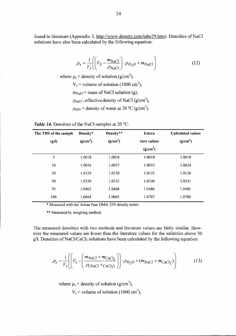
found in literature (Appendix 3, http://www.densitv.com/tabe29.htm). Densities ofNaCI solutions have also been calculated by the following equation:
Ps = V1 ((Vs- mNaCl). PH20 + mNaCIJ s l PNaCl
where Ps = density of solution (g/cm3),
Vs = volume of solution (1000 cm3),
ffiNaCI = mass ofNaCI solution (g),
PNaCI = effective density ofNaCI (g/cm3),
PH20 = density ofwater at 20 oc (g/cm3).
Table 14. Densities ofthe NaCI-samples at 20 °C.
The TDS ofthe sample Density* Density** Litera
(g/1) (g/cm3) (g/cm3
) ture values
(g/cm3)
5 1.0018 1.0024 1.0018
10 1.0054 1.0057 1.0053
20 1.0124 1.0130 1.0125
50 1.0330 1.0332 1.0340
70 1.0463 1.0468 1.0486
100 1.0664 1.0665 1.0707
* Measured with the Anton Paar DMA 35N density meter.
* * Measured by weighing method.
(12)
Calculated values
1.0018
1.0054
1.0126
1.0341
1.0485
1.0700
The measured densities with two methods and literature values are fairly similar. However the measured values are lower than the literature values for the salinities above 50 g/1. Densities ofNaCl/CaCh solutions have been calculated by the following equation:
(13)
where Ps = density of solution (g/cm3),
Vs = volume ofsolution (1000 cm3),

25
ffiNaCI = mass ofNaCl (g),
mcaCI2 = mass of CaCh (g),
PCNaCI+ caCI2) = effective density of solution where 50% is NaCl and 50 % is CaCh (g/cm3
),
PH2o = density ofwater at 20 oc (g/cm3).
Table 15. Densities ofthe NaCl/CaCh-samples at 20 °C.
The TDS of the sample Density* Density** Calculated values
(g/1) (g/cm3) (g/cm3
) (g/cm3)
5 1.0022 1.0026 1.0022
10 1.0060 1.0064 1.0061
20 1.0135 1.0138 1.0139
50 1.0358 1.0358 1.0375
70 1.0505 1.0498 1.0532
100 1.0722 1.0711 1.0768
* Measured with the Anton Paar DMA 35N
* * Measured by weighing method.
As in case for the pure NaCl solutions the density values measured for the mixed NaCl/CaC12 samples were fairly similar at lower salinities and deviated from calculated values at higher salinities (TDS > 50 g/1).
Densities of the NaCl- and NaCl/CaCh-solutions were measured at the five stable temperatures: 16.5/17.5, 20, 25, 30 and 35 °C. Temperature coefficients for the solutions were calculated from the results. All coefficients are very small. If the temperature changes by 1 oc it only affects to the 4 th decimal of the density result. Pure NaClsolutions have somewhat higher temperature coefficients than NaCl/CaCb-solutions. Calculated temperature coefficients are not affected by the concentration of the solution. Small changes to density for solutions of different concentrations are quite small and within error limits of the calculations and measurements.

26
8. SUMMARY
Electrical conductivity of a solution is dependent on its temperature. Conductivities are measured at ambient temperature in the field with an on-line measuring system and thus in order to get comparable results a temperature correction must be used. Most commercially available conductivity meters have several temperature correction methods for different solutions. The aim of this study was to provide a data set to determine temperature correction coefficients for the ground waters from Olkiluoto and Hästholmen. The other aim was to study how temperature affects density measurements. Two different methods to measure density was also discussed.
Ali temperature correction coefficients for the electrical conductivity measurements were smaller than 2 %/°C, which is the most commonly used coefficient in the literature (for example: Kolthoff et al. 1978, Sundholm et al. 1978, Willard et al. 1981 ). The effect of the concentration of the solution on the temperature coefficient was examined by defining temperature coefficients in the concentration range 0-1 00 g/1. It was noticed that the temperature coefficient decreases when the concentration of the solution is increasing. Temperature coefficients, which were scoped in this study, take into account the real nature and concentration of deep groundwater samples.
Posiva's conductivity meters, which are used in on-line field measurements, have automatic temperature correction to the reference temperature for different kind of samples. Corrections are based on the intemational standards. Y okogawa' s meter has automatic temperature compensation according to standard NaCl curves. The correction coefficient is 2.1 %fOC when the conductivity of the sample is < 10 S/m. It is also possible to program an own linear temperature compensation factor to the meter. It must be between -1 0 - + 1 0 %!°C. The conductivity meter of Kemotron has six temperature correction curves. We have used the compensation based on NaCl solutions curves and the numerical value is 2.1 %/°C. Also for Kemotron meter an own temperature coefficient can be used. These must be between 0-9.9 %!°C. Electrical conductivity of all Posiva's groundwater samples is also measured in the laboratory. Automatic temperature compensation is used and the value is 2.14 %fOC.
Effect of sulphate on temperature correction coefficient of the N aCl solution could not be evaluated in this study, because of different TDS values of the solutions. When TDS is different the solutions act slightly different to the changes in the temperature. Differences between the temperature coefficients of the NaCl and NaCl/Na2S04 solutions are small. Ifthe difference between the TDS ofthe solutions would be larger, the difference between temperature coefficient would be larger too.
Density at 20 oc of the water samples was measured by two different methods. Density values obtained with Anton Paar DMA35 density meter and weighing Method were almost the same. With increasing concentration of the measured solution the difference between the measured values and literature values is increasing too. Density of the NaCl/CaCh-solutions are slightly higher than the density of the NaCl-solutions al-
27
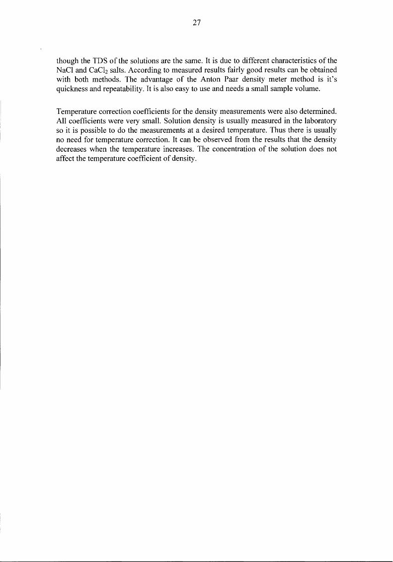
though the TDS of the solutions are the same. It is due to different characteristics of the NaCl and CaCh salts. According to measured results fairly good results can he ohtained with hoth methods. The advantage of the Anton Paar density meter method is it's quickness and repeatahility. It is also easy to use and needs a small sample volume.
Temperature correction coefficients for the density measurements were also determined. Ali coefficients were very small. Solution density is usually measured in the lahoratory so it is possihle to do the measurements at a desired temperature. Thus there is usually no need for temperature correction. It can he ohserved from the results that the density decreases when the temperature increases. The concentration of the solution does not affect the temperature coefficient of density.

28
9. REFERENCES
Annual book of ASTM Standards, 1986. Water and Environmental Technology: Water (1), vol. 11.01, American Society for Testing and Materials, USA.
Forsythe, W. E. 1956. Smithsonian physical tables, 9th edition, The Lord Baltimore Press, USA, p. 397.
Foxboro Company, 1987. Theory and application of electrolytic conductivity measurement, Technical Information, TI 612-112, USA.
Gray, D. M. & Bevilacqua, A. C. 1999. Evaluating cation conductivity temperature compensation, Ultrapure water, UP160460, 1999, p. 60-64.
Herbst, K. 1998. Anton Paar GmbH, Austria.
Jameel, R., Wu, Y. & Pratt, K. 2000. Primary standardsandstandard reference materials for electrolytic conductivity, NIST Special Publication 260-142.
Karttunen, V. 2000. Review on the deviations in the analytical results of Posiva's groundwater samples, Working Report 2000-34, Posiva Oy (ln Finnish with English abstract).
Kolthoff, M. (editor) & Elving, P. J. (editor) 1978. Treatise on analytical chemistry: Part 1. Theory and practise vol. 4, 2 nd edition, John Wiley and Sons, New York, 1978.
Mäntynen, M. 1998. Measuring of the pH, electrical conductivity and dissolved oxygen from saline groundwater, Pro Gradu-työ, Jyväskylän Yliopisto (in Finnish).
Mäntynen, M. 2000. Calculating the temperature coefficient for electric conductivity measurements and some observations of the connection between TDS and electric conductivity, Working Report 2000-16, Posiva Oy (ln Finnish with English abstract).
Radiometer Copenhagen, CMD230 Conductivity meter: Operating Instructions, D21M009.
Ranta, E. & Tiilikainen, M. 1991. Lukion taulukot, WSOY, Porvoo.
SFS-EN27888, 1994. Water quality: Determination of electrical conductivity, Painokartano Ky, Helsinki (ln Finnish).
Sundholm, G., Raitanen, E., Hakoila, E., Asplund, J., Lindström, M. & Steinby, K. 1978. Instrumentalanalysis II: Electrochemical analyse, Vammalan kirjapaino, 1978 (In Finnish).
Willard, H. H., Merrit, L. L., Dean, J. A. & Settle, F. A., 1981. Instrumental methods of analysis, 6th edition, Wadsworth Publishing Company, Califomia, p. 781-783.
29
Zabarsky, 0. 1992. Temperature-compensated conductivity-a necessity for measuring high- purity water, Ultrapure water, UP090156, p. 56-59.
Vuorinen, U. & Snellman, M. 1998. Finnish reference waters for solubility, sorption and diffusion studies, Working report 98-61, Posiva Oy.

31
APPENDIX 1: TEMPERATURE CORRECTION COEFFICIENTS OF THE NATURAL WATERS FROM THE SFS-STANDARD
9 f25 oc .0 .1 .2 .3 .4 .5 .6 .7 .8 .9 0 1.918 1.912 1.906 1.899 1.893 1.887 1.881 1.875 1.869 1.863 1 1.857 1.851 1.845 1.840 1.834 1.829 1.822 1.817 1.811 1.805 2 1.800 1.794 1.788 1.783 1.777 1.772 1.766 1.761 1.756 1.750 3 1.745 1.740 1.734 1.729 1.724 1.719 1.713 1.708 1.703 1.698 4 1.693 1.688 1.683 1.678 1.673 1.668 1.663 1.658 1.653 1.648 5 1.643 1.638 1.634 1.629 1.624 1.619 1.615 1.610 1.605 1.601 6 1.596 1.591 1.587 1.582 1.578 1.573 1.596 1.564 1.560 1.555 7 1.551 1.547 1.542 1.538 1.534 1.529 1.525 1.521 1.516 1.512 8 1.508 1.504 1.500 1.496 1.491 1.487 1.483 1.479 1.475 1.471 9 1.467 1.463 1.459 1.455 1.451 1.447 1.443 1.439 1.436 1.432 10 1.428 1.424 1.420 1.416 1.413 1.409 1.405 1.401 1.398 1.394 11 1.390 1.387 1.383 1.379 1.376 1.372 1.369 1.365 1.362 1.358 12 1.354 1.351 1.347 1.344 1.341 1.337 1.334 1.330 1.327 1.323 13 1.320 1.317 1.313 1.310 1.307 1.303 1.300 1.297 1.294 1.290 14 1.287 1.824 1.281 1.278 1.274 1.271 1.268 1.265 1.262 1.259 15 1.256 1.253 1.249 1.246 1.243 1.240 1.237 1.234 1.231 1.228 16 1.225 1.222 1.219 1.216 1.214 1.211 1.208 1.205 1.202 1.199 17 1.196 1.193 1.191 1.188 1.185 1.182 1.179 1.177 1.174 1.171 18 1.168 1.166 1.163 1.160 1.157 1.155 1.152 1.149 1.147 1.144 19 1.141 1.139 1.136 1.134 1.131 1.128 1.126 1.123 1.121 1.118 20 1.116 1.113 1.111 1.108 1.105 1.103 1.101 1.098 1.096 1.093 21 1.091 1.088 1.086 1.083 1.081 1.079 1.076 1.074 1.071 1.069 22 1.067 1.064 1.062 1.060 1.057 1.055 1.053 1.051 1.048 1.046 23 1.044 1.041 1.039 1.037 1.035 1.032 1.030 1.028 1.026 1.024 24 1.021 1.019 1.017 1.015 1.013 1.011 1.008 1.006 1.004 1.002 25 1.000 0.998 0.996 0994 0.992 0.990 0.987 0.985 0.983 0.981 26 0.979 0.977 0.975 0.973 0.971 0.969 0.967 0.965 0.963 0.961 27 0.959 0.957 0.955 0.953 0.952 0.950 0.948 0.946 0.944 0.942 28 0.940 0.938 0.936 0.934 0.933 0.931 0.929 0.927 0.925 0.923 29 0.921 0.920 0.918 0.916 0.914 0.912 0.911 0.909 0.907 0.905 30 0.903 0.902 0.900 0.898 0.896 0.895 0.893 0.891 0.889 0.888 31 0.886 0.884 0.883 0.881 0.879 0.877 0.876 0.874 0.872 0.871 32 0.869 0.867 0.866 0.864 0.863 0.861 0.859 0.858 0.856 0.854 33 0.853 0.851 0.850 0848 0.846 0.845 0.843 0.842 0.840 0.839 34 0.837 0.835 0.834 0.832 0.831 0.829 0.828 0.826 0.825 0.823 35 0.822 0.820 0.819 0.817 0.816 0.914 0.813 0.811 0.810 0.808

32
APPENDIX 2: DENSITY OF WATER (g/Cm3) FROM 0 TO 40 OC
0,0 0,1 0,2 0,3 0,4 0,5 0,6 0,7 0,8 0,9
0 .99984 .99985 .99985 .99986 .99987 .99987 .99988 .99988 .99989 .99989 .99990 .99990 .99991 .99991 .99992 .99992 .99993 .99993 .99993 .99994
2 .99994 .99994 .99995 .99995 .99995 .99995 .99996 .99996 .99996 .99996 3 .99996 .99997 .99997 .99997 .99997 .99997 .99997 .99997 .99997 .99997 4 .99997 .99997 .99997 .99997 .99997 .99997 .99997 .99997 .99997 .99997 5 .99996 .99996 .99996 .99996 .99996 .99995 .99995 .99995 .99995 .99994 6 .99994 .99994 .99993 .99993 .99993 .99992 .99992 .99991 .99991 .99991 7 .99990 .99990 .99989 .99989 .99988 .99988 .99987 .99987 .99986 .99986 8 .99985 .99984 .99984 .99983 .99982 .99982 .99981 .99980 .99980 .99979 9 .99978 .99977 .99977 .99976 .99975 .99974 .99973 .99973 .99972 .99971 10 .99970 .99969 .99968 .99967 .99966 .99965 .99964 .99963 .99962 .99961 11 .99960 .99959 .99958 .99957 .99956 .99955 .99954 .99953 .99952 .99951 12 .99950 .99949 .99947 .99946 .99945 .99944 .99943 .99941 .99940 .99939 13 .99938 .99936 .99935 .99934 .99933 .99931 .99930 .99929 .99927 .99926 14 .99924 .99923 .99922 .99920 .99919 .99917 .99916 .99914 .99913 .99911 15 .99910 .99908 .99907 .99905 .99904 .99902 .99901 .99899 .99897 .99896 16 .99894 .99893 .99891 .99889 .99888 .99886 .99884 .99883 .99881 .99879 17 .99877 .99876 .99874 .99872 .99870 .99869 .99867 .99865 .99863 .99861 18 .99859 .99858 .99856 .99854 .99852 .99850 .99848 .99846 .99844 .99842 19 .99840 .99838 .99836 .99835 .99833 .99831 .99828 .99826 .99824 .99822 20 .99820 .99818 .99816 .99814 .99812 .99810 .99808 .99806 .99803 .99801 21 .99799 .99797 .99795 .99793 .99790 .99788 .99786 .99784 .99781 .99779 22 .99777 .99775 .99772 .99770 .99768 .99765 .99763 .99761 .99758 .99756 23 .99754 .99751 .99749 .99747 .99744 .99742 .99739 .99737 .99734 .99732 24 .99730 .99727 .99725 .99722 .99720 .99717 .99715 .99712 .99709 .99707 25 .99704 .99702 .99699 .99697 .99694 .99691 .99689 .99686 .99683 .99681 26 .99678 .99676 .99673 .99670 .99667 .99665 .99662 .99659 .99657 .99654 27 .99651 .99648 .99646 .99643 .99640 .99637 .99634 .99632 .99629 .99626 28 .99623 .99620 .99617 .99615 .99612 .99609 .99606 .99603 .99600 .99597 29 .99594 .99591 .99588 .99585 .99582 .99579 .99577 .99574 .99571 .99568 30 .99564 .99561 .99558 .99555 .99552 .99549 .99546 .99543 .99540 .99537 31 .99534 .99531 .99528 .99524 .99521 .99518 .99515 .99512 .99509 .99506 32 .99502 .99499 .99469 .99493 .99490 .99486 .99483 .99480 .99477 .99473 33 .99470 .99467 .99463 .99460 .99457 .99454 .99450 .99447 .99444 .99440 34 .99473 .99433 .99430 .99427 .99423 .99420 .99417 .99413 .99410 .99406 35 .99403 .99399 .99396 .99393 .99389 .99386 .99382 .99379 .99375 .99372 36 .99368 .99365 .99361 .99358 .99354 .99350 .99347 .99343 .99340 .99336 37 .99333 .99329 .99325 .99322 .99318 .99314 .99311 .99307 .99304 .99300 38 .99296 .99292 .99289 .99285 .99281 .99278 .99274 .99270 .99267 .99263 39 .99259 .99255 .99252 .99248 .99244 .99240 .99236 .99233 .99229 .99225 40 .99221 .99217 .99214 .99210 .99206 .99202 .99198 .99194 .99190 .99186
33
APPENDIX 3: DENSITIES OF NaCI SOLUTIONS AT 20 °C
(Reference: httQ://www.density.com/tabe29.htm)
ffiNaCI Density IDNaCI Density ffiNaCI Density
(g) (g/cm3) (g) (g/cm3
) (g) (g/cm3)
0.9989 33 1.0218 80 1.0559
2 0.9997 34 1.0225 82 1.0574
3 1.0004 35 1.0232 84 1.0588
4 1.0011 36 1.0239 86 1.0603
5 1.0018 37 1.0246 88 1.0618
6 1.0025 38 1.0254 90 1.0633
7 1.0032 39 1.0261 92 1.0647
8 1.0039 40 1.0268 94 1.0662
9 1.0046 41 1.0275 96 1.0677
10 1.0053 42 1.0282 98 1.0692
11 1.0060 43 1.0290 100 1.0707
12 1.0068 44 1.0297 105 1.0744
13 1.0075 45 1.0304 110 1.0781
14 1.0082 46 1.0311 115 1.0819
15 1.0089 47 1.0318 120 1.0837
16 1.0096 48 1.0326 125 1.0894
17 1.0103 49 1.0333 130 1.0932
18 1.0110 50 1.034 135 1.0970
19 1.0117 52 1.0355 140 1.1008
20 1.0125 54 1.0369 145 1.1047
21 1.0132 56 1.0384 150 1.1085
22 1.0139 58 1.098 160 1.1162
23 1.0146 60 1.0413 170 1.1240
24 1.0153 62 1.0427 180 1.1319
25 1.0160 64 1.0442 190 1.1398
26 1.0168 66 1.0456 200 1.1478
27 1.0175 68 1.0471 210 1.1558
28 1.0182 70 1.0486 220 1.1640
29 1.0189 72 1.0500 230 1.1721
30 1.0196 74 1.0515 240 1.1804
31 1.0203 76 1.0530 250 1.1887
32 1.0211 78 1.0544 260 1.9272
34
APPENDIX 4: DENSITIES OF CaCI2 SOLUTIONS AT 20 °C
(reference: http://www.density.com/tabe29.htm)
m CaCI 2
Density mCaCI2 Density
(g) (g/cm3) (g) (g/cm3
)
5 1.0024 110 1.0923
10 1.0065 120 1.1014
15 1.0106 130 1.1105
20 1.0148 140 1.1198
25 1.0190 150 1.1292
30 1.0232 160 1.1386
35 1.0274 170 1.1482
40 1.0316 180 1.1579
45 1.0358 190 1.1677
50 1.0401 200 1.1775
55 1.0443 220 1.1976
60 1.0486 240 1.2180
65 1.0529 260 1.2388
70 1.0572 280 1.2600
75 1.0615 300 1.2816
80 1.0659 320 1.3036
85 1.0703 340 1.3260
90 1.0747 360 1.3488
95 1.0791 380 1.3720
100 1.0835 400 1.3957

35
APPENDIX 5: TEMPERATURE COEFFICIENT OF THE DENSITY MEAS-UREMENTS FOR THE SAMPLES WITH A TDS = 5 g/1 CALCULATED BY USING THE POL YNOMIAL
NaCI-sample N aCI/CaCh-sample Temperature Density Temperature Density Temperature
(oC) (glcm3) coefficient (g/cm3
) coefficient (g/cm3°C) (gc/m3°C}
5 1.0040 -0.00015 1.0050 -0.00018
6 1.0039 -0.00016 1.0049 -0.00018
7 1.0038 -0.00016 1.0048 -0.00018
8 1.0037 -0.00017 1.0046 -0.00018
9 1.0036 -0.00017 1.0045 -0.00019
10 1.0035 -0.00018 1.0043 -0.00019
11 1.0034 -0.00019 1.0041 -0.00019
12 1.0032 -0.00019 1.0040 -0.00020
13 1.0031 -0.00019 1.0038 -0.00020
14 1.0029 -0.00020 1.0036 -0.00020
15 1.0027 -0.00020 1.0034 -0.00021
16 1.0025 -0.00021 1.0032 -0.00021
17 1.0023 -0.00022 1.0030 -0.00021
18 1.0021 -0.00022 1.0028 -0.00021
19 1.0019 -0.00022 1.0026 -0.00022
20 1.0017 1.0024
21 1.0015 0.00023 1.0022 0.00022
22 1.0012 0.00024 1.0019 0.00023
23 1.0010 0.00025 1.0017 0.00023
24 1.0007 0.00025 1.0015 0.00023
25 1.0004 0.00026 1.0012 0.00023
26 1.0001 0.00026 1.0010 0.00024
27 0.9998 0.00027 1.0007 0.00024
28 0.9995 0.00027 1.0004 0.00024
29 0.9992 0.00028 1.0002 0.00025
30 0.9989 0.00028 0.9999 0.00025
31 0.9986 0.00029 0.9996 0.00025
32 0.9982 0.00029 0.9993 0.00026
33 0.9979 0.00030 0.9990 0.00026
34 0.9975 0.00030 0.9987 0.00026
35 0.9971 0.00031 0.9984 0.00026

36
APPENDIX 6: TEMPERATURE COEFFICIENT OF THE DENSITY MEAS-UREMENTS FOR THE SAMPLES WITH A TDS = 10 g/1 CALCULATED BY USING THE POL YNOMIAL
NaCI-sample NaCI/CaCh-sample Temperature Density Temperature Density Temperature
ec) (g/cm3) coefficient (glcm3
) coefficient (g/cm3°C) (g/cm3°C)
5 1.0078 -0.00017 1.0090 -0.00018
6 1.0077 -0.00017 1.0089 -0.00018
7 1.0076 -0.00017 1.0088 -0.00018
8 1.0075 -0.00018 1.0086 -0.00018
9 1.0073 -0.00019 1.0085 -0.00019
10 1.0072 -0.00019 1.0083 -0.00019
11 1.0071 -0.00019 1.0081 -0.00019
12 1.0069 -0.00020 1.0080 -0.00020
13 1.0067 -0.00020 1.0078 -0.00020
14 1.0066 -0.00021 1.0076 -0.00020
15 1.0064 -0.00021 1.0074 -0.00021
16 1.0062 -0.00022 1.0072 -0.00021
17 1.0060 -0.00022 1.0070 -0.00021
18 1.0058 -0.00023 1.0068 -0.00021
19 1.0055 -0.00023 1.0066 -0.00022
20 1.0053 1.0064
21 1.0051 0.00025 1.0062 0.00001
22 1.0048 0.00025 1.0059 0.00002
23 1.0045 0.00026 1.0057 0.00003
24 1.0043 0.00026 1.0055 0.00004
25 1.0040 0.00027 1.0052 0.00005
26 1.0037 0.00027 1.0050 0.00006
27 1.0034 0.00028 1.0047 0.00006
28 1.0031 0.00028 1.0044 0.00007
29 1.0027 0.00029 1.0042 0.00008
30 1.0024 0.00029 1.0039 0.00009
31 1.0021 0.00030 1.0036 0.00009
32 1.0017 0.00030 1.0033 0.00010
33 1.0013 0.00031 1.0030 0.00011
34 1.0010 0.00031 1.0027 0.00011
35 1.0006 0.00032 1.0024 0.00012
37
APPENDIX 7: TEMPERATURE COEFFICIENT OF THE DENSITY MEAS-UREMENTS FOR THE SAMPLES WITH A TDS = 20 g/1 CALCULATED BY USING THE POL YNOMIAL
N aCI-sample NaCI/CaCh-sample Temperature Density Temperature Density Temperature
(OC) (g/cm3) coefficient (g/cm3
) coefficient (g/cm3°C) (g/cmJoct)
5 1.0156 -0.00018 1.0164 -0.00020
6 1.0155 -0.00018 1.0163 -0.00020
7 1.0154 -0.00018 1.0161 -0.00021
8 1.0152 -0.00018 1.0159 -0.00021
9 1.0151 -0.00019 1.0158 -0.00022
10 1.0149 -0.00019 1.0156 -0.00022
11 1.0147 -0.00019 1.0154 -0.00022
12 1.0146 -0.00020 1.0152 -0.00023
13 1.0144 -0.00020 1.0150 -0.00023
14 1.0142 -0.00020 1.0148 -0.00024
15 1.0140 -0.00021 1.0146 -0.00024
16 1.0138 -0.00021 1.0144 -0.00024
17 1.0136 -0.00021 1.0141 -0.00025
18 1.0134 -0.00021 1.0139 -0.00025
19 1.0132 -0.00022 1.0137 -0.00026
20 1.0130 1.0134
21 1.0128 0.00022 1.0131 0.00001
22 1.0125 0.00023 1.0129 0.00003
23 1.0123 0.00023 1.0126 0.00004
24 1.0121 0.00023 1.0123 0.00005
25 1.0118 0.00023 1.0120 0.00006
26 1.0116 0.00024 1.0117 0.00007
27 1.0113 0.00024 1.0114 0.00008
28 1.0110 0.00024 1.0111 0.00009
29 1.0108 0.00025 1.0107 0.00010
30 1.0105 0.00025 1.0104 0.00010
31 1.0102 0.00025 1.0101 0.00011
32 1.0099 0.00026 1.0097 0.00012
33 1.0096 0.00026 1.0093 0.00013
34 1.0093 0.00026 1.0090 0.00013
35 1.0090 0.00026 1.0086 0.00014

38
APPENDIX 8: TEMPERATURE COEFFICIENT OF THE DENSITY MEAS-UREMENTS FOR THE SAMPLES WITH A TDS = 50 g/1 CALCULATED BY USING THE POL YNOMIAL
NaCI-sample NaCI/CaCh-sample Temperature Density Temperature Density Temperature
(OC) (g/cm3) coefficient (g/cm3
) coefficient (wcm3°C) (wcm3°C)
5 1.0382 -0.00035 1.0399 -0.00025
6 1.0378 -0.00035 1.0396 -0.00025
7 1.0374 -0.00035 1.0394 -0.00025
8 1.0370 -0.00034 1.0392 -0.00026
9 1.0367 -0.00034 1.0389 -0.00026
10 1.0363 -0.00034 1.0387 -0.00026
11 1.0359 -0.00034 1.0385 -0.00026
12 1.0356 -0.00034 1.0382 -0.00026
13 1.0352 -0.00033 1.0380 -0.00027
14 1.0349 -0.00033 1.0377 -0.00027
15 1.0346 -0.00033 1.0375 -0.00027
16 1.0342 -0.00033 1.0372 -0.00027
17 1.0339 -0.00033 1.0369 -0.00027
18 1.0335 -0.00032 1.0367 -0.00028
19 1.0332 -0.00032 1.0364 -0.00028
20 1.0329 1.0361
21 1.0326 0.00032 1.0358 0.00001
22 1.0323 0.00032 1.0355 0.00003
23 1.0320 0.00031 1.0352 0.00004
24 1.0317 0.00031 1.0349 0.00005
25 1.0314 0.00031 1.0347 0.00006
26 1.0311 0.00031 1.0343 0.00007
27 1.0308 0.00031 1.0340 0.00008
28 1.0305 0.00030 1.0337 0.00009 29 1.0302 0.00030 1.0334 0.00010
30 1.0299 0.00030 1.0331 0.00010
31 1.0296 0.00030 1.0328 0.00011
32 1.0293 0.00030 1.0325 0.00012
33 1.0291 0.00029 1.0321 0.00012
34 1.0288 0.00029 1.0318 0.00013
35 1.0286 0.00029 1.0315 0.00014
39
APPENDIX 9: TEMPERATURE COEFFICIENT OF THE DENSITY MEAS-UREMENTS FOR THE SAMPLES WITH A TDS = 70 g/1 CALCULATED BY USING THE POL YNOMIAL
NaCI-sample NaCI/CaCh-sample Temperature Density Temperature Density Temperature
(OC) (glcm3) coefficient (g/cm3
) coefficient {g/cm3°C) (g/cm3°C)
5 1.0524 -0.00048 1.0552 -0.00025
6 1.0519 -0.00047 1.0549 -0.00025
7 1.0513 -0.00047 1.0547 -0.00025
8 1.0508 -0.00046 1.0545 -0.00026
9 1.0503 -0.00045 1.0542 -0.00026
10 1.0498 -0.00045 1.0540 -0.00026
11 1.0493 -0.00045 1.0538 -0.00026
12 1.0488 -0.00044 1.0535 -0.00026
13 1.0483 -0.00043 1.0533 -0.00027
14 1.0479 -0.00043 1.0530 -0.00027
15 1.0474 -0.00042 1.0528 -0.00027
16 1.0470 -0.00042 1.0525 -0.00027
17 1.0465 -0.00041 1.0522 -0.00027
18 1.0461 -0.00041 1.0520 -0.00028
19 1.0457 -0.00040 1.0517 -0.00028
20 1.0453 1.0514
21 1.0449 0.00039 1.0511 0.00001
22 1.0445 0.00039 1.0508 0.00003
23 1.0441 0.00039 1.0505 0.00004
24 1.0438 0.00038 1.0502 0.00005
25 1.0434 0.00038 1.0500 0.00006
26 1.0431 0.00037 1.0496 0.00007
27 1.0427 0.00037 1.0493 0.00008
28 1.0424 0.00036 1.0490 0.00009
29 1.0421 0.00036 1.0487 0.00010
30 1.0418 0.00035 1.0484 0.00010
31 1.0415 0.00034 1.0481 0.00011
32 1.0412 0.00034 1.0478 0.00012
33 1.0409 0.00033 1.0474 0.00012
34 1.0407 0.00033 1.0471 0.00013
35 1.0404 0.00032 1.0468 0.00014

40
APPENDIX 10: TEMPERATURE COEFFICIENT OF THE DENSITY MEAS-UREMENTS FOR THE SAMPLES WITH A TDS = 100 g/1 CALCULATED BY USING THE POL YNOMIAL
N aCI-sample NaCI/CaCh-sample Temperature Density Temperature Density Temperature
(OC) (g/cm3) coefficient (g/cm3
) coefficient {g/cm3°C) {g/cm3°C)
5 1.0729 -0.00045 1.0784 -0.00050
6 1.0723 -0.00044 1.0779 -0.00050
7 1.0718 -0.00044 1.0774 -0.00050
8 1.0713 -0.00043 1.0769 -0.00050
9 1.0708 -0.00043 1.0764 -0.00050
10 1.0703 -0.00042 1.0759 -0.00050
11 1.0698 -0.00041 1.0754 -0.00050
12 1.0694 -0.00041 1.0749 -0.00050
13 1.0689 -0.00040 1.0744 -0.00050
14 1.0685 -0.00040 1.0739 -0.00050
15 1.0681 -0.00039 1.0734 -0.00050
16 1.0676 -0.00038 1.0729 -0.00050
17 1.0672 -0.00038 1.0724 -0.00050
18 1.0668 -0.00037 1.0719 -0.00050
19 1.0665 -0.00037 1.0714 -0.00050
20 1.0661 1.0709
21 1.0657 0.00035 1.0704 0.00002
22 1.0654 0.00035 1.0699 0.00005
23 1.0651 0.00034 1.0694 0.00007
24 1.0648 0.00034 1.0689 0.00009
25 1.0645 0.00033 1.0685 0.00010
26 1.0642 0.00032 1.0680 0.00012
27 1.0639 0.00032 1.0675 0.00013
28 1.0636 0.00031 1.0670 0.00015
29 1.0633 0.00031 1.0665 0.00016
30 1.0631 0.00030 1.0660 0.00017
31 1.0629 0.00029 1.0655 0.00018
32 1.0626 0.00029 1.0650 0.00019
33 1.0624 0.00028 1.0645 0.00020
34 1.0622 0.00028 1.0640 0.00021
35 1.0621 0.00027 1.0635 0.00022