HAL Id: hal-01255774https://hal.archives-ouvertes.fr/hal-01255774

Submitted on 14 Jan 2016

HAL is a multi-disciplinary open accessarchive for the deposit and dissemination of sci-entific research documents, whether they are pub-lished or not. The documents may come fromteaching and research institutions in France orabroad, or from public or private research centers.

L’archive ouverte pluridisciplinaire HAL, estdestinée au dépôt et à la diffusion de documentsscientifiques de niveau recherche, publiés ou non,émanant des établissements d’enseignement et derecherche français ou étrangers, des laboratoirespublics ou privés.

TARGET-FREE EXTRINSIC CALIBRATION OF AMOBILE MULTI-BEAM LIDAR SYSTEM

H Nouira, Jean-Emmanuel Deschaud, F Goulette

To cite this version:H Nouira, Jean-Emmanuel Deschaud, F Goulette. TARGET-FREE EXTRINSIC CALIBRATIONOF A MOBILE MULTI-BEAM LIDAR SYSTEM. Laserscanning, Geospatial week 2015, Sep 2015,La grande Motte, France. �10.5194/isprsannals-II-3-W5-97-2015�. �hal-01255774�

TARGET-FREE EXTRINSIC CALIBRATION OF A MOBILE MULTI-BEAM LIDARSYSTEM

H. Nouiraa, J. E. Deschauda, F. Goulettea

a MINES ParisTech, PSL - Research University, CAOR - Center for Robotics, 60 Bd St-Michel 75006 Paris, France -(houssem.nouira, jean-emmanuel.deschaud, francois.goulette)@mines-paristech.fr

Commission III, WG III/2

KEY WORDS: LIDAR, Calibration, Mobile Mapping, 3D, Automatic, Computer Processing, Velodyne

ABSTRACT:

LIDAR sensors are widely used in mobile mapping systems. With the recent developments, the sensors provide high amounts of data,which are necessary for some applications that require a high level of detail. Multi-beam LIDAR sensors can provide this level ofdetail, but need a specific calibration routine to provide the best precision possible. Because they have many beams, the calibration ofsuch sensors is difficult and is not well represented in the litterature.We present an automatic method for the optimization of the calibration parameters of a multi-beam LIDAR sensor: the proposedapproach does not need any calibration target, and only uses information from the acquired point clouds, which makes it simple to use.For our optimization method, we define an energy function which penalizes points far from local planar surfaces. At the end of theautomatic process, we are able to give the precision of the calibration parameters found.

1. INTRODUCTION

Light Detection and Ranging (LIDAR) sensors are useful for manytasks: mapping (Nuchter et al., 2004), localization (NarayanaK. S et al., 2009) and autonomous driving (Grand Darpa Chal-lenge, 2007) are some of the applications in which such sensorsare used. Recently, multi-beam LIDAR sensors have appeared:they are more precise and give point clouds with high densitiesof points. In order to give correctly geo-referenced data withsensors mounted on a mobile platform, additional informationfrom exteroceptive and proprioceptive sensors are needed. Also,the calibration of the whole system is required; however, it ismostly done with calibration targets, and needs human interven-tion, as for example with the system presented in (Huang andBarth, 2009). The calibration can take some time, and it is diffi-cult to evaluate the precision of the method. The whole processof acquisition and data geo-referencement is illustrated with fig-ure 1, with the different representations of each acquired point.In this article, we call calibration of the multi-beam LIDAR sen-sor its extrinsic calibration: it consists in finding the rigid trans-formation between the LIDAR sensor and the IMU, so that thedata acquired by the sensor are correctly projected in the naviga-tion reference frame.The solution we propose is, after the acquisition, to estimate theparameters of the calibration that give the ”best” - depending onsome criteria - point cloud. We present an unsupervised extrinsiccalibration method for multi-beam LIDAR sensors, which doesnot need any calibration target. We start with an initial calibra-tion, which does not need to be close to the true one. With an iter-ative process, we look for ”better” calibration parameters, whichimprove the quality of the point clouds and minimize an energyfunction we will define in section 3..This method does apply forany multi-beam sensor mounted on a mobile platform (a vehicleor a robot), and retrieves the six extrinsic parameters - three oftranslation and three of rotation - of the transformation betweenthe sensor and the IMU.This paper is organized as follow: in section 2., we present thestate of the art concerning the algorithms for the calibration ofmulti-beam LIDAR sensors. Section 3. presents our calibration

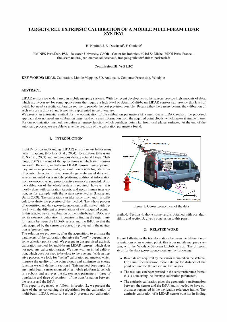
Figure 1: Geo-referencement of the data

method. Section 4. shows some results obtained with our algo-rithm, and section 5. gives a conclusion to this paper.

2. RELATED WORK

Figure 1 illustrates the transformations between the different rep-resentations of an acquired point: this is our mobile mapping sys-tem, with the Velodyne 32-beam LIDAR sensor. The differentsteps for the data geo-referencement are the following:

• Raw data are acquired by the sensor mounted on the Vehicle.For a multi-beam sensor, these data are the distance of thepoint acquired to the sensor and two angles

• The raw data can be expressed in the sensor reference frame:this is done using the intrinsic calibration parameters.

• The extrinsic calibration gives the geometric transformationbetween the sensor and the IMU, and is needed to have co-ordinates registered in the navigation reference frame. Theextrinsic calibration of a LIDAR sensor consists in finding

the transformation between the location on the mobile plat-form of the entire unit and the inertial measurement unit,also mounted on the mobile platform. There are six param-eters to retrieve, three rotations and three translations. Thisis the calibration we want to optimize, and in this article, wewill call calibration this extrinsic calibration.

• The data are geo-referenced by applying the transformationbetween the navigation reference frame and the world refer-ence frame to these data.

Multi-beam LIDAR sensors appeared recently, and calibrationtechniques for this kind of LIDAR sensors already exist. If wetake a look at the Velodyne sensor, some intrinsic calibrationmethods exist, like (Glennie and Lichti, 2010) and (Muhammadand Lacroix, 2010), which propose an optimization of the in-trinsic parameters of the 64-beam version, or (Chan and Lichti,2013), which proposes an intrinsic calibration for the 32-beammodel.In this paper, we are only interested in the extrinsic calibration ofmulti-beam LIDAR sensors. In (Zhu and Liu, 2013), the authorspropose a method to optimize the 3 parameters of rotation intotwo steps: first, the roll and pitch angles by estimating groundplanes, and after, the yaw angle by matching pole-like obstacles.This method is unsupervised and does not need a calibration tar-get, as it uses only information from the data gathered; but, thelimitation is that it only estimates the rotation parameters, anddoes not take into account the translation ones. In (Huang et al.,2013), the authors propose a full extrinsic calibration of a multi-beam LIDAR sensor, but they use calibration targets and infraredimages to do this task. Also, in (Elseberg et al., 2013), the au-thors want to optimize the calibration of the whole system theyuse, which is composed of several LIDAR sensors. The energyfunction is a sum of Point Density Functions, which measures thecompactness of their point clouds. They use an unsupervised andtarget-free method in post-processing, where an energy functionthey defined is minimized. The energy function was constructedin order to measure the compactness of the point clouds acquired.Finally, some approaches optimize both the intrinsic and the ex-trinsic calibration of a LIDAR sensor at the same time. This is thecase in (Levinson and Thrun, 2010), where the authors presentan intrinsic calibration and an extrinsic calibration method whichuses the same energy function to minimize. For both calibrations,the authors chose an energy function which penalizes points thatare far away from planar surfaces extracted from the acquireddata. As in (Elseberg et al., 2013), this is a post-processing op-timization, which is unsupervised and target-free. In (Levinsonand Thrun, 2010), the authors start from an initial extrinsic cal-ibration estimate, and iteratively compute values of their energyfunction by modifying the six extrinsic parameters in the neigh-borhood of the initialization. They use a grid search to optimizethe parameters - for the minimization process, they alternativelytest the translation parameters and the rotation parameters be-cause of the difference of dimensionality -, and reduce the sizeof the neighborhood at each iteration. The main problem is thatthe minimization can be long if a high precision is required. Also,because the neighborhood is a discrete space, we possibly do notreach the optimal solution.To optimize the calibration parameters of the multi-beam sensor,we use an energy function only using information extracted fromthe acquired point clouds.No calibration target is used, and the process is unsupervised.The defined energy function is also minimized iteratively, as itwill be explained in section 3.2.2. However, the differences withrespect to existing methods are manyfold:

• First, the energy is defined as the sum of the squared dis-tance of each points to the closest plane it should belong to,

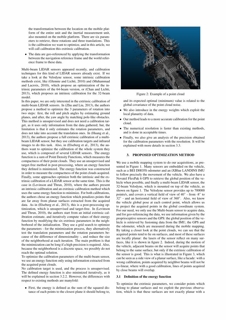
Figure 2: Example of a point cloud

and its expected optimal (minimum) value is related to theglobal covariance of the point cloud noise.

• We also introduce in the energy weights which exploit thelocal planarity of data.

• Our method leads to a more accurate calibration for the pointcloud.

• The numerical resolution is faster than existing methods,and is done in acceptable times.

• Finally, we also give an analysis of the precision obtainedfor the calibration parameters with the resolution. It will beexplained with more details in section 3.3.

3. PROPOSED OPTIMIZATION METHOD

We use a mobile mapping system to do our acquisitions, as pre-sented in Figure 1. Many sensors are embedded on the vehicle,such as a BEI DHO5S odometer and an iXBlue LANDINS IMUto follow precisely the movement of the vehicle. We also have aNovatel FlexPak 6 GPS to retrieve the global position of the ve-hicle when possible, and finally a multi-beam LIDAR sensor, the32-beam Velodyne, which is mounted on top of the vehicle, asshown on figure 1. The Velodyne sensor provides up to 700000points/s, and covers a vertical field of view of 40◦ - from -8◦ to32◦ - and an horizontal field of view of 360◦. Also, we knowthe vehicle global pose at each control point, which allows usto project the acquired points in the global coordinate system.For our need, we only use the Multi-beam sensor to acquire data,and for geo-referencing the data, we use information given by theproprioceptive sensors and the GPS: the global position of the ve-hicle is retrieved by fusioning data from the IMU, the GPS andthe odometer, which are measured during the mobile mapping.By taking a closer look at the point clouds, we can see that theacquired points tend to lie on surfaces, and most of these surfacesare locally planar: the lasers of the sensor reflect on many sur-faces, like it is shown in figure 2. Indeed, during the motion ofthe vehicle, adjacent beams on the sensor will acquire points thatbelong to the same surface, but only if the extrinsic calibration ofthe sensor is good. This is what is illustrated in Figure 3, whichcan be seen as a side view of a planar surface, like a facade: with awrong calibration, points acquired by neighbor beams will not beco-linear, where with a good calibration, lines of points acquiredby close beams will overlap.

3.1 Definition of the energy function

To optimize the extrinsic parameters, we consider points whichbelong to planar surfaces and we exploit the previous observa-tion, which is that these surfaces are not exactly planar with a

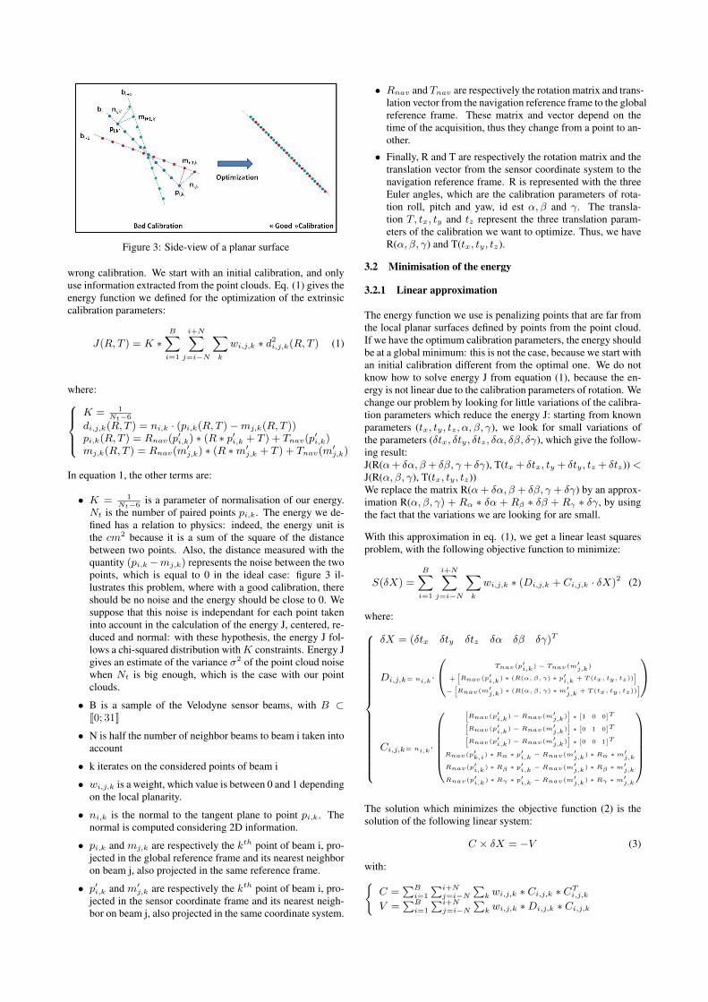
Figure 3: Side-view of a planar surface

wrong calibration. We start with an initial calibration, and onlyuse information extracted from the point clouds. Eq. (1) gives theenergy function we defined for the optimization of the extrinsiccalibration parameters:

J(R, T ) = K ∗B∑i=1

i+N∑j=i−N

∑k

wi,j,k ∗ d2i,j,k(R, T ) (1)

where:K = 1

Nt−6

di,j,k(R, T ) = ni,k · (pi,k(R, T )−mj,k(R, T ))pi,k(R, T ) = Rnav(p

′i,k) ∗ (R ∗ p′i,k + T ) + Tnav(p

′i,k)

mj,k(R, T ) = Rnav(m′j,k) ∗ (R ∗m′j,k + T ) + Tnav(m

′j,k)

In equation 1, the other terms are:

• K = 1Nt−6

is a parameter of normalisation of our energy.Nt is the number of paired points pi,k. The energy we de-fined has a relation to physics: indeed, the energy unit isthe cm2 because it is a sum of the square of the distancebetween two points. Also, the distance measured with thequantity (pi,k−mj,k) represents the noise between the twopoints, which is equal to 0 in the ideal case: figure 3 il-lustrates this problem, where with a good calibration, thereshould be no noise and the energy should be close to 0. Wesuppose that this noise is independant for each point takeninto account in the calculation of the energy J, centered, re-duced and normal: with these hypothesis, the energy J fol-lows a chi-squared distribution withK constraints. Energy Jgives an estimate of the variance σ2 of the point cloud noisewhen Nt is big enough, which is the case with our pointclouds.

• B is a sample of the Velodyne sensor beams, with B ⊂J0; 31K

• N is half the number of neighbor beams to beam i taken intoaccount

• k iterates on the considered points of beam i

• wi,j,k is a weight, which value is between 0 and 1 dependingon the local planarity.

• ni,k is the normal to the tangent plane to point pi,k. Thenormal is computed considering 2D information.

• pi,k and mj,k are respectively the kth point of beam i, pro-jected in the global reference frame and its nearest neighboron beam j, also projected in the same reference frame.

• p′i,k and m′j,k are respectively the kth point of beam i, pro-jected in the sensor coordinate frame and its nearest neigh-bor on beam j, also projected in the same coordinate system.

• Rnav and Tnav are respectively the rotation matrix and trans-lation vector from the navigation reference frame to the globalreference frame. These matrix and vector depend on thetime of the acquisition, thus they change from a point to an-other.

• Finally, R and T are respectively the rotation matrix and thetranslation vector from the sensor coordinate system to thenavigation reference frame. R is represented with the threeEuler angles, which are the calibration parameters of rota-tion roll, pitch and yaw, id est α, β and γ. The transla-tion T, tx, ty and tz represent the three translation param-eters of the calibration we want to optimize. Thus, we haveR(α, β, γ) and T(tx, ty, tz).

3.2 Minimisation of the energy

3.2.1 Linear approximation

The energy function we use is penalizing points that are far fromthe local planar surfaces defined by points from the point cloud.If we have the optimum calibration parameters, the energy shouldbe at a global minimum: this is not the case, because we start withan initial calibration different from the optimal one. We do notknow how to solve energy J from equation (1), because the en-ergy is not linear due to the calibration parameters of rotation. Wechange our problem by looking for little variations of the calibra-tion parameters which reduce the energy J: starting from knownparameters (tx, ty, tz, α, β, γ), we look for small variations ofthe parameters (δtx, δty, δtz, δα, δβ, δγ), which give the follow-ing result:J(R(α+ δα, β+ δβ, γ+ δγ), T(tx+ δtx, ty + δty, tz + δtz)) <J(R(α, β, γ), T(tx, ty, tz))We replace the matrix R(α+ δα, β + δβ, γ + δγ) by an approx-imation R(α, β, γ) + Rα ∗ δα + Rβ ∗ δβ + Rγ ∗ δγ, by usingthe fact that the variations we are looking for are small.

With this approximation in eq. (1), we get a linear least squaresproblem, with the following objective function to minimize:

S(δX) =

B∑i=1

i+N∑j=i−N

∑k

wi,j,k ∗ (Di,j,k + Ci,j,k · δX)2 (2)

where:

δX = (δtx δty δtz δα δβ δγ)T

Di,j,k= ni,k·

Tnav(p′i,k) − Tnav(m′j,k)

+[Rnav(p′i,k) ∗ (R(α, β, γ) ∗ p′i,k + T (tx, ty, tz))

]−[Rnav(m′j,k) ∗ (R(α, β, γ) ∗m′j,k + T (tx, ty, tz))

]

Ci,j,k= ni,k·

[Rnav(p′i,k) − Rnav(m′j,k)

]∗[1 0 0

]T[Rnav(p′i,k) − Rnav(m′j,k)

]∗[0 1 0

]T[Rnav(p′i,k) − Rnav(m′j,k)

]∗[0 0 1

]TRnav(p′k,i) ∗ Rα ∗ p

′i,k − Rnav(m′j,k) ∗ Rα ∗m′j,k

Rnav(p′i,k) ∗ Rβ ∗ p′i,k − Rnav(m′j,k) ∗ Rβ ∗m

′j,k

Rnav(p′i,k) ∗ Rγ ∗ p′i,k − Rnav(m′j,k) ∗ Rγ ∗m′j,k

The solution which minimizes the objective function (2) is thesolution of the following linear system:

C × δX = −V (3)

with:{C =

∑Bi=1

∑i+Nj=i−N

∑k wi,j,k ∗ Ci,j,k ∗ C

Ti,j,k

V =∑Bi=1

∑i+Nj=i−N

∑k wi,j,k ∗Di,j,k ∗ Ci,j,k

3.2.2 Optimization approach

To find the optimal calibration parameters, we compute δX it-eratively, until the calibration parameters converge. At each newiteration n+1, the calibration parameters are defined as follow:

txn+1 = txn + δtxntyn+1 = tyn + δtyntzn+1 = tzn + δtznαn+1 = αn + δαnβn+1 = βn + δβnγn+1 = γn + δγn

(4)

As it is presented in the next section 3.3, C is an important matrixwhich helps us get an estimate of the precision of the calibrationparameters retrieved through optimization.We start the optimization process with initial calibration param-eters (tx0 , ty0 , tz0 , α0, β0, γ0), and at each iteration, to find thenew variations δX , we minimize the objective function (2). Wewill see in section 4. that the initial calibration can be far from thetrue one, and that we do not need a precise estimate to start with.The complete algorithm is presented in algorithm 1.The stop criterion we chose concerns the variation of δX dur-ing the iterations: the algorithm stops when ‖δX‖max is under athreshold δ, or after a certain number of iterations.

3.3 Precision of the calibration parameters

In the state of the art of the calibration of mobile mapping sys-tems, there is no value given to measure the precision of theoptimized parameters: the authors generally compare their re-sult point clouds to a ground truth, which can be hard and time-consuming, because the ground truth cannot be done with an au-tomatic process; human supervision is needed to validate the pro-cess. In our method, we give values to measure the precision ofthe parameters retrieved with our optimization process: we havean estimate of the precision for each parameter, given by the fol-lowing terms:

{For translations: σx(m) =

√(C−1)1,1

For rotations: σα(rad) =√

(C−1)4,4(5)

The remaining precisions are defined the same way for the trans-lations and rotations parameters. C is the matrix defined in eq.(3), and its inverse C−1 = Cov(δX). With the square roots, wehave the precisions of each parameter.These precision depend on the structure of the point cloud andthe trajectory of the vehicle. For example:

• a point cloud with some features, such as turns or a variationof altitude, will give a better precision for the calibrationparameters.

• a trajectory which goes straight, without changes, will notgive a good precision for the parameters.

3.4 Validity of the calibration

We defined in the previous sections an energy function that, withan optimization process, should gives better calibration parame-ters for our points clouds. We will discuss in this section about thecondition that validate a calibration obtained with our optimiza-tion process. The value of the energy J should be small enough,under a threshold: as said in section 3.1, our energy follows achi-squared distribution with Nt − 6 constraints. A validationthreshold at 97% is 3σ2, with σ2 the variance of the point cloudnoise. For example, for real data, the noise comes from the acqui-sitions, but also the IMU and the GPS which give the trajectory

Algorithm 1: Iterative linear optimization for the parameters ofthe extrinsic calibration

Data: A point cloud, with an initial calibration, and a knowntrajectory

Result: A point cloud, with optimized calibration parametersReading and sub-sampling of the point cloud;Initial extrinsic calibration;repeat

Global referencing of the points acquired with the actualcalibration (txn , tyn , tzn , αn, βn, γn);Selection of the points pi,k;Construction of the pair of points pi,k from beam i andmj,k, their closest neighbor from beam j;Computation of the normals to each planes at points pi,k;Construction of equation (3), and resolution which gives thevariations (δtxn , δtyn , δtzn , δαn, δβn, δγn);

until ‖δX‖max < δ, or niter ≥ nmax;Saving of the modified point cloud with the optimizedcalibration;

of the vehicle; with our mobile mapping system, we have a goodprecision, with a standard deviation for the noise around 5cm. Itgives us a threshold of around 75 cm2 for the value of energy J.

4. EXPERIMENTS

4.1 Datasets

In our experiments, we used two types of data: synthetic andreal point clouds. The difference between them concerns the waythe point cloud is ”created”: for synthetic data, we simulated anacquisition in a urban area, with vertical planes as walls and anhorizontal plane as the ground. For real data, we used our mobilemapping platform to acquire point clouds in a city. But, otherthan that, we use the same informations for both data. We haveraw informations from the sensor, which is composed of:

• the position of the vehicle at each acquisition instant. This isthe position of the IMU in the world reference frame, fusedwith other informations from proprioceptives sensors, suchas the GPS and the odometer.

• the coordinates of each acquired point in the spherical coor-dinate system of the sensor reference frame.

• the ”beam” which acquired each point, since we work witha multi-beam sensor.

These informations give us the position of the vehicle and its tra-jectory with a high precision: indeed, we only work on the cal-ibration of the LIDAR sensor, and to have a well reconstructedpoint cloud at the end of the optimization, the trajectory has to beknown precisely.

4.2 Implementation and algorithm parameters

The algorithm we presented was implemented in C++. The EIGENlibrary (Eigen library, 2014) was used for all the operations onmatrices or vectors, and the FLANN library (FLANN library,2014) (Fast Library for Approximated Nearest Neighbor) wasused for the nearest neighbors search. The algorithms runs ona computer with a Windows 7 - 64 bits os, 32 GB of RAM and anintel core-i7 processor, with a clock up to 3.40 GHz.Our algorithm was tested with synthetic and real urban data: forthe synthetic data, the parameters were known precisely. For thereal data, we didn’t know the true calibration: for both data, we

tx(cm) ty(cm) tz(cm) α(◦) β(◦) γ(◦)Initial calibration -200.00 240.00 -150.00 5.00 -37.00 -5.50

Difference between the ground truth and the state-of-the-art optimization 0.00 400.00 -50.00 -0.25 0.00 -0.25Difference between the ground truth and our optimization 0.00 0.02 0.02 0.00 -0.01 0.06

Table 4: Optimization of the calibration of synthetic point cloud #1

tx(cm) ty(cm) tz(cm) α(◦) β(◦) γ(◦)Initial calibration -200.00 240.00 -150.00 5.00 -7.00 -5.50

Difference between the ground truth and the state-of-the-art optimization 240.23 640.23 190.23 0.01 0.01 6.09Difference between the ground truth and our optimization 0.01 -0.13 -200.00 -0.01 0.00 -0.00

Table 5: Optimization of the calibration of synthetic point cloud #2

σtx (cm) σty (cm) σtz (cm) σα(◦) σβ(◦) σγ(◦)Synthetic point cloud #1 1.49 3.43 5.58 0.97 0.05 0.10Synthetic point cloud #2 0.78 3.51 1.00 ∗ 1020 0.04 0.05 0.05

Table 6: Precision of the parameters found for the simulated data

Figure 7: Synthetic point cloud #1: on top, with the initial cali-bration; middle, with a state of the art optimization; at the bottom,with our optimization. The three images have the same point ofview.

started with an initial calibration arbitrarily chosen.In our algorithm, we have some parameters to set. We start withsub-sampling the data about 1 point out of 2, because the pointclouds have a high resolution and in order to reduce the com-putation times and the use of memory. The number of neigh-bor beams for a beam bi was fixed to 4 (N=2). Concerning theweights wi,j,k, a threshold of 20 cm was chosen for the maximaldistance between a point pi,k and its nearest neighbormj,k on theneighbor beam. We also considered that all the points belongedto planar surfaces, because the real point clouds presented in thissection were acquired in a urban environment. Finally, the num-ber of closest neighbors Ncn taken into account for the search ofthe neighbor mj,k of point pi,k was set to 100.The parameters were fixed for all the tests which were done: dif-ferent values were tested, but the ones presented give the bestoptimization results and computation times.

4.3 Comparison to the state of the art

We compared our approach and results with the optimization pre-sented in (Levinson and Thrun, 2010), where the calibration of

Figure 8: Synthetic point cloud #2: on top, before optimization ofthe calibration; middle, with a state of the art optimization; at thebottom, after our optimization. The three images have the samepoint of view.

a Velodyne sensor is also being optimized automatically. Theenergy function used and the optimization method are different:their method is a discrete search of the optimal parameters in theneighborhood of their starting calibration. They try several com-bination of parameters value to find the optimal calibration forthe sensor, and repeat the process iteratively with reducing thespace of search. They also separate the search for the translationparameters first, and then for the rotation parameters.They set various parameters in their algorithm, which are:

• the size of the neighborhood for the optimization; it reduceswith each iteration, until they have the needed precision forthe parameters.

• a step of discretization - different or not from a parameterto an other -, which is the ”number” of values tested in theirneighborhood for each parameter.

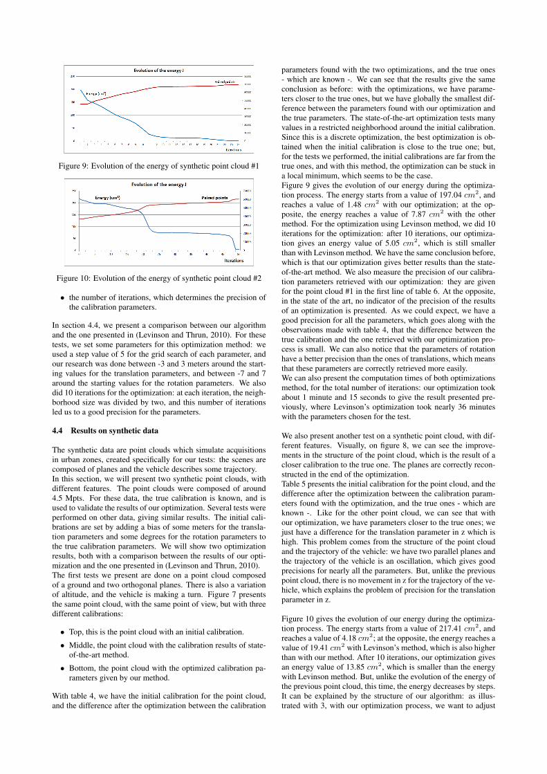
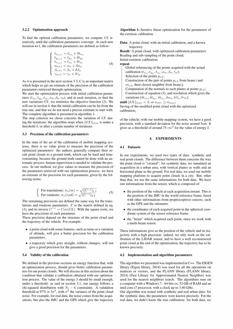
Figure 9: Evolution of the energy of synthetic point cloud #1

Figure 10: Evolution of the energy of synthetic point cloud #2

• the number of iterations, which determines the precision ofthe calibration parameters.

In section 4.4, we present a comparison between our algorithmand the one presented in (Levinson and Thrun, 2010). For thesetests, we set some parameters for this optimization method: weused a step value of 5 for the grid search of each parameter, andour research was done between -3 and 3 meters around the start-ing values for the translation parameters, and between -7 and 7around the starting values for the rotation parameters. We alsodid 10 iterations for the optimization: at each iteration, the neigh-borhood size was divided by two, and this number of iterationsled us to a good precision for the parameters.

4.4 Results on synthetic data

The synthetic data are point clouds which simulate acquisitionsin urban zones, created specifically for our tests: the scenes arecomposed of planes and the vehicle describes some trajectory.In this section, we will present two synthetic point clouds, withdifferent features. The point clouds were composed of around4.5 Mpts. For these data, the true calibration is known, and isused to validate the results of our optimization. Several tests wereperformed on other data, giving similar results. The initial cali-brations are set by adding a bias of some meters for the transla-tion parameters and some degrees for the rotation parameters tothe true calibration parameters. We will show two optimizationresults, both with a comparison between the results of our opti-mization and the one presented in (Levinson and Thrun, 2010).The first tests we present are done on a point cloud composedof a ground and two orthogonal planes. There is also a variationof altitude, and the vehicle is making a turn. Figure 7 presentsthe same point cloud, with the same point of view, but with threedifferent calibrations:

• Top, this is the point cloud with an initial calibration.

• Middle, the point cloud with the calibration results of state-of-the-art method.

• Bottom, the point cloud with the optimized calibration pa-rameters given by our method.

With table 4, we have the initial calibration for the point cloud,and the difference after the optimization between the calibration

parameters found with the two optimizations, and the true ones- which are known -. We can see that the results give the sameconclusion as before: with the optimizations, we have parame-ters closer to the true ones, but we have globally the smallest dif-ference between the parameters found with our optimization andthe true parameters. The state-of-the-art optimization tests manyvalues in a restricted neighborhood around the initial calibration.Since this is a discrete optimization, the best optimization is ob-tained when the initial calibration is close to the true one; but,for the tests we performed, the initial calibrations are far from thetrue ones, and with this method, the optimization can be stuck ina local minimum, which seems to be the case.Figure 9 gives the evolution of our energy during the optimiza-tion process. The energy starts from a value of 197.04 cm2, andreaches a value of 1.48 cm2 with our optimization; at the op-posite, the energy reaches a value of 7.87 cm2 with the othermethod. For the optimization using Levinson method, we did 10iterations for the optimization: after 10 iterations, our optimiza-tion gives an energy value of 5.05 cm2, which is still smallerthan with Levinson method. We have the same conclusion before,which is that our optimization gives better results than the state-of-the-art method. We also measure the precision of our calibra-tion parameters retrieved with our optimization: they are givenfor the point cloud #1 in the first line of table 6. At the opposite,in the state of the art, no indicator of the precision of the resultsof an optimization is presented. As we could expect, we have agood precision for all the parameters, which goes along with theobservations made with table 4, that the difference between thetrue calibration and the one retrieved with our optimization pro-cess is small. We can also notice that the parameters of rotationhave a better precision than the ones of translations, which meansthat these parameters are correctly retrieved more easily.We can also present the computation times of both optimizationsmethod, for the total number of iterations: our optimization tookabout 1 minute and 15 seconds to give the result presented pre-viously, where Levinson’s optimization took nearly 36 minuteswith the parameters chosen for the test.

We also present another test on a synthetic point cloud, with dif-ferent features. Visually, on figure 8, we can see the improve-ments in the structure of the point cloud, which is the result of acloser calibration to the true one. The planes are correctly recon-structed in the end of the optimization.Table 5 presents the initial calibration for the point cloud, and thedifference after the optimization between the calibration param-eters found with the optimization, and the true ones - which areknown -. Like for the other point cloud, we can see that withour optimization, we have parameters closer to the true ones; wejust have a difference for the translation parameter in z which ishigh. This problem comes from the structure of the point cloudand the trajectory of the vehicle: we have two parallel planes andthe trajectory of the vehicle is an oscillation, which gives goodprecisions for nearly all the parameters. But, unlike the previouspoint cloud, there is no movement in z for the trajectory of the ve-hicle, which explains the problem of precision for the translationparameter in z.

Figure 10 gives the evolution of our energy during the optimiza-tion process. The energy starts from a value of 217.41 cm2, andreaches a value of 4.18 cm2; at the opposite, the energy reaches avalue of 19.41 cm2 with Levinson’s method, which is also higherthan with our method. After 10 iterations, our optimization givesan energy value of 13.85 cm2, which is smaller than the energywith Levinson method. But, unlike the evolution of the energy ofthe previous point cloud, this time, the energy decreases by steps.It can be explained by the structure of our algorithm: as illus-trated with 3, with our optimization process, we want to adjust

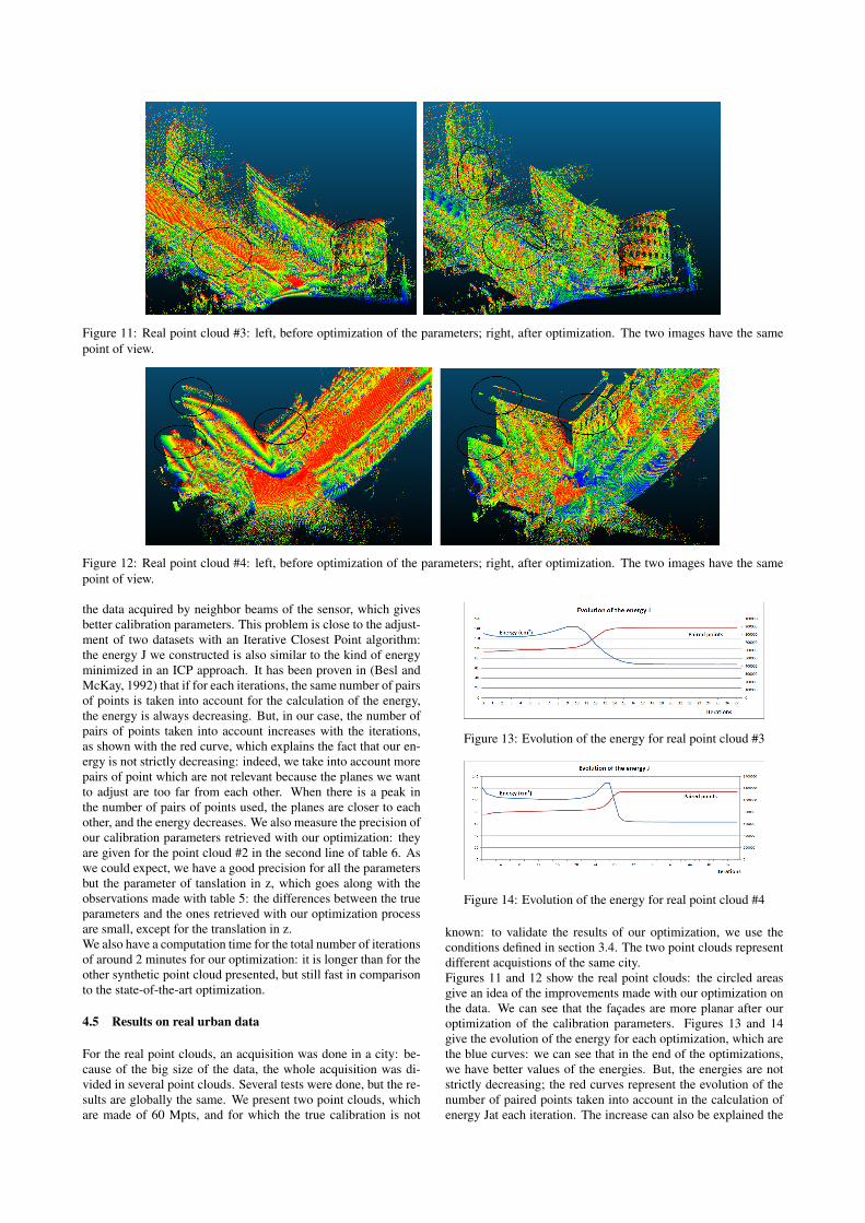
Figure 11: Real point cloud #3: left, before optimization of the parameters; right, after optimization. The two images have the samepoint of view.

Figure 12: Real point cloud #4: left, before optimization of the parameters; right, after optimization. The two images have the samepoint of view.

the data acquired by neighbor beams of the sensor, which givesbetter calibration parameters. This problem is close to the adjust-ment of two datasets with an Iterative Closest Point algorithm:the energy J we constructed is also similar to the kind of energyminimized in an ICP approach. It has been proven in (Besl andMcKay, 1992) that if for each iterations, the same number of pairsof points is taken into account for the calculation of the energy,the energy is always decreasing. But, in our case, the number ofpairs of points taken into account increases with the iterations,as shown with the red curve, which explains the fact that our en-ergy is not strictly decreasing: indeed, we take into account morepairs of point which are not relevant because the planes we wantto adjust are too far from each other. When there is a peak inthe number of pairs of points used, the planes are closer to eachother, and the energy decreases. We also measure the precision ofour calibration parameters retrieved with our optimization: theyare given for the point cloud #2 in the second line of table 6. Aswe could expect, we have a good precision for all the parametersbut the parameter of tanslation in z, which goes along with theobservations made with table 5: the differences between the trueparameters and the ones retrieved with our optimization processare small, except for the translation in z.We also have a computation time for the total number of iterationsof around 2 minutes for our optimization: it is longer than for theother synthetic point cloud presented, but still fast in comparisonto the state-of-the-art optimization.

4.5 Results on real urban data

For the real point clouds, an acquisition was done in a city: be-cause of the big size of the data, the whole acquisition was di-vided in several point clouds. Several tests were done, but the re-sults are globally the same. We present two point clouds, whichare made of 60 Mpts, and for which the true calibration is not

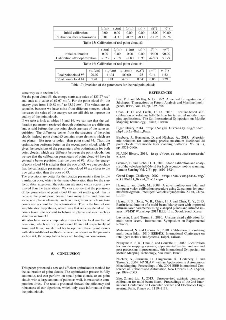
Figure 13: Evolution of the energy for real point cloud #3

Figure 14: Evolution of the energy for real point cloud #4

known: to validate the results of our optimization, we use theconditions defined in section 3.4. The two point clouds representdifferent acquistions of the same city.Figures 11 and 12 show the real point clouds: the circled areasgive an idea of the improvements made with our optimization onthe data. We can see that the facades are more planar after ouroptimization of the calibration parameters. Figures 13 and 14give the evolution of the energy for each optimization, which arethe blue curves: we can see that in the end of the optimizations,we have better values of the energies. But, the energies are notstrictly decreasing; the red curves represent the evolution of thenumber of paired points taken into account in the calculation ofenergy Jat each iteration. The increase can also be explained the

tx(m) ty(m) tz(m) α(◦) β(◦) γ(◦)Initial calibration 0.00 0.00 0.00 0.00 -45.00 90.00

Calibration after optimization 0.01 -1.37 -0.32 -8.11 -61.25 99.78

Table 15: Calibration of real point cloud #3

tx(m) ty(m) tz(m) α(◦) β(◦) γ(◦)Initial calibration 0.00 0.00 0.00 0.00 -45.00 90.00

Calibration after optimization -0.23 -1.39 -2.80 0.99 -62.03 91.79

Table 16: Calibration of real point cloud #4

σtx(cm) σty(cm) σtz(cm) σα(◦) σβ(◦) σγ(◦)Real point cloud #3 20.07 11.04 100.00 1.75 0.14 1.52Real point cloud #4 2.41 1.81 47.51 0.34 0.05 0.29

Table 17: Precision of the parameters for the real point clouds

same way as in section 4.4.For the point cloud #3, the energy starts at a value of 125.27 cm2

and ends at a value of 67.67 cm2. For the point cloud #4, theenergy goes from 110.88 cm2 to 63.37 cm2. The values are ac-ceptable, because we have noise from different sources, whichincreases the value of the energy: we are still able to improve thequality of the point clouds.If we take a look at tables 15 and 16, we can see that the cal-ibration parameters retrieved through optimization are different;but, as said before, the two point clouds are part of the same ac-quisition. The difference comes from the structure of the pointclouds: indeed, point cloud #3 contains more elements which arenot planar - like trees or poles - than point cloud #4. Thus, theoptimization performs better on the second point cloud: table 17gives the precisions of the parameters after optimization for bothpoint clouds, which are different between the point clouds; butwe see that the calibration parameters of point cloud #4 have ingeneral a better precision than the ones of #3. Also, the energyof point cloud #4 is smaller than the one of #3: we can concludethat the calibration parameters of point cloud #4 are closer to thetrue calibration than the ones of #3.The precisions are better for the rotation parameters than for thetranslation ones, which is the same observation than for the syn-thetic data: in general, the rotations are more easily correctly re-trieved than the translations. We can also see that the precisionsof the parameters of point cloud #3 are not really good: this isbecause the point cloud doesn’t have many turns, and there aresome non planar elements, such as trees, from which we takepoints into account for the optimization. This is the limit of oursimplification hypothesis, which was that we considered all thepoints taken into account to belong to planar surfaces, such asstated in section 3.1.We also have some computation times for the total number ofiterations, which are for point cloud #3 and #4 respectively of7min and 8min: we did not try to optimize these point cloudswith state-of-the-art methods because, as shown in the previoussection 4.4, the computation times are too high in comparison.

5. CONCLUSION

This paper presented a new and efficient optimization method forthe calibration of point clouds. The optimization process is fullyautomatic, and can perform on small point clouds, or on pointclouds with a large amount of points as well, in reasonable com-putation times. The results presented showed the efficiency androbustness of our algorithm, which only uses information fromthe point clouds.

REFERENCES

Besl, P. J. and McKay, N. D., 1992. A method for registration of3d shapes. Transactions on Pattern Analysis and Machine Intelli-gence, IEEE, Vol. 14, pp. 239–256.

Chan, T. O. and Lichti, D. D., 2013. Feature-based self-calibration of velodyne hdl-32e lidar for terrestrial mobile map-ping applications. The 8th International Symposium on MobileMapping Technology, Tainan, Taiwan.

Eigen library, 2014. http://eigen.tuxfamily.org/index.php?title=Main_Page.

Elseberg, J., Borrmann, D. and Nuchter, A., 2013. Algorith-mic solutions for computing precise maximum likelihood 3dpoint clouds from mobile laser scanning platforms. Vol. 5(11),pp. 5871–5906.

FLANN library, 2014. http://www.cs.ubc.ca/research/flann.

Glennie, C. and Lichti, D. D., 2010. Static calibration and analy-sis of the velodyne hdl-64e s2 for high accuracy mobile scanning.Remote Sensing Vol. 2(6), pp. 1610–1624.

Grand Darpa Challenge, 2007. http://en.wikipedia.org/wiki/DARPA_Grand_Challenge.

Huang, L. and Barth, M., 2009. A novel multi-planar lidar andcomputer vision calibration procedure using 2d patterns for auto-mated navigation. Intelligent Vehicles Symposium, Xi’an, China,IEEE.

Huang, P. S., Hong, W. B., Chien, H. J. and Chen, C. Y., 2013.Extrinsic calibration of a multi-beam lidar system with improvedintrinsic laser parameters using v-shaped planes and infrared im-ages. IVMSP Workshop, 2013 IEEE 11th, Seoul, South Korea.

Levinson, J. and Thrun, S., 2010. Unsupervised calibration formulti-beam lasers. International Symposium on ExperimentalRobotics.

Muhammad, N. and Lacroix, S., 2010. Calibration of a rotatingmulti-beam lidar. 2010 IEEE/RSJ International Conference onIntelligent Robots and Systems, Taipei, Taiwan.

Narayana K. S, K., Choi, S. and Goulette, F., 2009. Localizationfor mobile mapping systems, experimental results, analysis andpost-processing improvements. 6th International Symposium onMobile Mapping Technology, Sao Paulo, Brazil.

Nuchter, A., Surmann, H., Lingemann, K., Hertzberg, J. andThrun, S., 2004. 6D SLAM with an Application in AutonomousMine Mapping. Proceedings of the 2004 IEEE International Con-ference on Robotics and Automation, New Orleans, L.A. (April),pp. 1998–2003.

Zhu, Z. and Liu, J., 2013. Unsupervised extrinsic parameterscalibration for multi-beam lidars. Proceedings of the 2nd Inter-national Conference on Computer Science and Electronics Engi-neering, Paris, France pp. 1110–1113.