Extrinsic Multi-Sensor Calibration For Mobile RobotsUsing the Gauss-Helmert Model

Kaihong Huang Cyrill Stachniss

Abstract— Most state estimation procedures in mobilerobotics require information about the locations of the indi-vidual sensors on the platform. This is especially the casewhen estimating geometric properties about the environmentor the robot. In this paper, we present an novel approachto extrinsic, multi-sensor calibration. Our approach seeks tofind the extrinsic parameters by maximizing the consistency ofthe motion estimate that is computed from different sensingmodalities. Our approach formulates constraints between themovements of the sensors using the Gauss-Helmert model. Thisallows us to compute a more accurate solution than the ordinaryleast squares approach. We implemented our approach andtested it using multiple sensors as well as when using a motioncapture studio. The experiments presented in this paper showthat our approach is able to accurately determine the extrinsicconfiguration of each sensor and is robust enough for typicallyapplications in mobile robotics.

I. INTRODUCTION

Most mobile robots perform some form of state estimationsuch as localization, mapping, SLAM, or exploration. Formost of such tasks, it is important to know where theindividual sensors are mounted on the robot. The task ofdetermining the position and orientation of a sensor is oftenreferred to extrinsic calibration. Without such calibrationinformation, a lot of the estimation tasks, especially thoserelated to computing geometric models such as SLAM, donot work properly and/or provide suboptimal results. Suchextrinsic calibration is also important when the informationfrom multiple sensors have to be fused.

In this paper, we address the problem of estimating theextrinsic parameters of multiple sensors relative to each otheror with respect to a base frame of a mobile robot. Ourcalibration approach is based on the robot’s motion and doesnot rely on external markers, calibration patterns, or a knownenvironment. We assume that each sensing modality allowsfor estimating a (relative) trajectory of the sensor giventhe observations. This holds for cameras by using visualodometry, for laser scanners or RGB-D cameras throughscan matching, and obviously for odometry as well as GPSreceivers. We do not address calibration for sensors that donot have this property such as a bumper sensor.

Our approach exploits constraints between the motionsof individual sensors and formulates the resulting error

All authors are with the University of Bonn, Institute of Geodesy andGeoinformation, Bonn, Germany.

This work has partly been supported by the DFG under the grant numberFOR-1015: Mapping on Demand as well as by the European Commissionunder the Horizon 2020 framework programme under grant agreement no.645403. Furthermore, we received support by the China Scholarship CouncilCSC.

minimization problem using the Gauss-Helmert model [18].This allows us to exploit constraints resulting from the factthat the sensors are rigidly mounted on the platform whilebeing able to handle noisy observations and compute aweighted least squares solution. This leads to a statisticallysound estimation providing accurate extrinsic calibrationparameters for multiple sensors and has the potential to yieldbetter results than traditional least squares.

The main contribution of this paper is a novel motion-based calibration algorithm for multiple sensors using theGauss-Helmert formulation. Our approach makes the as-sumptions that the sensors are rigidly attached to the robotand that a relative trajectory estimate can be obtained fromeach sensor. Under these assumptions, our approach (i) ac-curately determines the extrinsic calibration parameters, (ii)requires an initial guess with an accuracy that can be obtainedthrough a direct approach, (iii) obtains more accurate resultscompared to ordinary least squares using the Gauss-Markovmodel, and (iv) can be executed in a reasonable amount oftime to be useful for real world applications. These fourclaims are backed up through the paper and its experimentalevaluation.

II. RELATED WORK

The problem of multi-sensor extrinsic calibration ad-dressed in this paper is strongly related to the hand-eyecalibration problem [14], [15], [17]. Here, the unknowntransformation between a robotic arm and a rigidly mountedcamera is estimated given a series of relative pose measure-ments. Earlier work by Shiu and Ahmad [14] describes thisproblem as solving a homogeneous transform equation inthe form of AX = XB, which relates the relative motions(A,B) of two devices to the sensors’ relative transformation(X ). Several efficient closed form solutions are available, bydecoupling the rotation and translation estimation [14], [17],or by using dual-quaternions formulation to allow for theestimation of rotation and translation simultaneously [4]. Thedirect solutions are comparably simple and fast to compute,but they are also sensitive to noise. To improve robustnessand accuracy, Horaud and Dornaika [5] propose to jointlyoptimize rotation and translation with nonlinear optimization.A subsequent approach [15] proposes a metric on the specialEuclidean group SE(3) and a corresponding error model fornonlinear optimization. Finally, Zhao et al. [19] proposeusing a L∞ cost function and utilize convex optimizationapproach instead of common least squares formulation.

Beside general hand eye problem, there are also worksfocused on special calibration problems. Driven by the needs

(ra, ta)

(rb, tb)

(ηb, ξb)SaiSbi

Sai+1

Sbi+1

Fig. 1: Relative movement at time i. Given rotation and translationmeasurements (ra, ta) and (rb, tb) from two sensors, our task isto find an optimal estimation of parameter (ηb, ξb), which is therelative orientation and displacement of sensor A in B’s frame.

of information fusion between camera and odometry, camera-odometry calibration for cars and wheeled mobile robots isone of the many [7], [8], [3], [13]. Explicit motion-basedsensor calibration has also been addressed by Taylor andNieto [16] and also combined with the SLAM problem [9].Guo et al. [7] proposed a two-step analytical least squaressolution to estimate rotation and translation separately, with-out using any special hardware or known landmarks. Theapproach by Heng et al. follow the formulation of Guo etal. [7], but only use the direct solution as initial guess to anextensive least squares estimation problem including cameraand odometry poses, intrinsic and extrinsic parameters, aswell as 3D scene points. In contrast to that, Schneider etal. [13] reported an online recursive estimation approachusing Unscented Kalman filter.

To the best of our knowledge, no other work exists thatbases the optimization for motion-based calibration on theGauss-Helmert model, which jointly optimize the modelparameter and observations together, thereby taking the ob-servation noise into full account.

III. MOTION-BASED EXTRINSIC CALIBRATION

The goal of motion-based extrinsic sensor calibration is todetermine the position and orientation of each sensor withoutmarkers and only based on the motion of the platform. Thecalibration is done with respect ot a reference point, whereassuch reference point can be the robot’s odometry frame orone of the sensors.

Consider a robot that is equipped with M sensors, whichare rigidly attached to the robot. We index these sensors witha, b, . . . ,m and each sensor is assumed to provide a (noisy)relative motion estimate of the sensor. More precisely, ateach time-step i, we have a set of relative pose measurementsconsisting of angle-axis rotation r and translation t for eachsensor:

{(rai, tai), . . . , (rmi, tmi) | R(r) ∈ SO(3), t ∈ IR3}, (1)

with i = 1, . . . , N . Each motion is expressed relatively in anego-centric frame for each sensor, i.e. the sensor pose of theprevious timestep.

The objective is to estimate the fixed but unknown trans-formations between all the sensors. Without loss of general-ity, we define the sensor a as the base sensor and estimate

for each other sensor s ∈ {b, . . . ,m} the relative rotationand translation (ηs, ξs) of Sai under the frame of Sbi .

{(ηs, ξs) | R(ηs) ∈ SO(3), ξs ∈ IR3, s = b...m} (2)

If we choose Sa to be the base/odometry frame of therobot, the tuples (ηs, ξs) are a solution to the extrinsic multi-sensor calibration problem. A point in Sa, written as ap, canbe transfered to the sensor frame Sb by:

bp = R(ηb)ap+ ξb. (3)

Fig. 1 (left) depicts the geometry for this problem. Suc-cessive poses of a sensor pair form a virtual quadrilateral orvector loop, which leads to the hand-eye problem equation:

ξb + R(ηb)ta − R(rb)ξb − tb = 03 (4)

R(ηb)R(ra)R(ηb)TR(rb)

T = I3. (5)

IV. PROBLEM OF ORDINARY LEAST SQUARESFOR MOTION-BASED CALIBRATION

The solution provided by closed form method are usuallyfar from perfect due to the decoupling and simplified noiseassumption (see [6] p.179). It is therefore necessary toemploy an iterative refinement process by means of leastsquares estimation, which not only jointly optimizes ξ,η butalso take the full uncertainty relations into account.

A widely used method is to iteratively minimize aweighted sum of a squared error function, e.g. [7], [15]. Inour case it is:

argminη,ξ

∑i

‖cti‖2wti+ ‖cri‖2wri

(6)

with

cti := (I3 − R(rbi))ξ + R(q)tai − tbi (7)

cri := log(R(η)R(rai)R(η)TR(rbi)

T). (8)

where ‖c‖2w := cTWc and W being a positive definiteweight matrix. The form of cri may varies, alternativescan be a Frobenius norm of a full rotation matrix, or ofa quaternion [15].

A minimizing of this cost function is easy to implementwith the help of popular off-the-self optimizer such asg2o[10] or Ceres[1] and therefore it is prominent in thecurrent literature of calibration problems. An overlookedpoint in most works are the values of the weight matricesW ri,W ti in this formula. And as we will see in the followingdiscussion, there is a hidden assumption in this optimizationmodel, which will degrade the estimation accuracy when themeasurement noise-level is high, and therefore only suitablefor low noise situations.

Eq. (6)-(8) is a approach based on the Gauss-Markovmodel (GM for short). The principle behind the GM modelis the “Gauss-Markov” theorem, which says the least squaresestimate gives no bias and has minimal variance if thefunctional relation l = f(x) is linear and the weightsare chosen to be W = Σ−1ll . The Gauss-Markov theoremalso holds approximately for nonlinear function f if thevariances of the observations are small compared to the

second derivatives of the functions (see [6] p.79). For theGM model it is important that the observations (l) has tobe explicit functions of the unknown parameters (x), toguarantee statistical optimality.

To fit in the Gauss-Markov theorem, we see that theGM model is actually using the residual vectors cti andcri as their observation entities l rather than the originalmeasurements {rsi, tsi}. So the weight matrix W ri,W ti

should therefore take the inverse of the covariance matrixof the residual vectors, i.e. W ri = Σ−1cr , W ti = Σ−1ct . Sincecti and cri are functions of {rsi, tsi}, we can apply errorpropagation to Eq. (8)-(7) and obtain

Σcr ≈ JrΣrrJTr , Σct ≈ JtΣttJT

t + JrΣrrJTr (9)

where Jr := ∂cri

∂riand Jt := ∂cti

∂tiare the Jacobians, and

Σtt,Σrr are the covariance matrices of the measurementnoise. Given the correct weight matrices, we can proceedwith minimizing Eq. (6) and refine x iteratively.

An issue to point out is that (r, t) is fixed during thewhole estimation process and so are the Jacobians andthe linearized model. If there are significant errors in themeasurement, they will persist and result in a degradedestimation accuracy. This degradation is what we observedin the real world application and thus motivated the workof this paper, its effect is confirmed by our experiment inSec. VI.

V. GAUSS-HELMERT-BASED APPROACHTO MULTI-SENSOR CALIBRATION

To tackle the aforementioned degradation problem in highnoise situation, we propose to formulate the estimationproblem using the Gauss-Helmert model [18], which makescorrections to not only the unknown parameters but also theobservations at each iteration.

The Gauss-Helmert model is more general than the GMmodel, it allow us to handle constraints between observation land unknown parameters x by implicit functions of the formg(x, l) = 0. It is closely related to the total-least-squaresmethod or the errors-in-variables method developed in statis-tics. Instead of minimizing residuals in the constraints, theGauss-Helmert model strictly enforces the constraints andmakes corrections to not only the unknown parameters butalso the observations. The objective is then to minimize thecorrections to the observation while estimating the unknownparameters.

Gauss-Markov and Gauss-Helmert model are equivalentfor problems in which observations are explicit functions ofthe unknown parameters, e.g l = f(x), because in thosecases the corrections to the parameters x are essentiallycorrections to the observation and so all the constraints areautomatically satisfied. However, Eq. (4) and Eq. (5) for(ξ,η) are obviously not in this explicit form.

A. Model for Multiple Sensors

Most related works consider only the formulation for twosensor, assuming we can simply apply the 2-sensor case toeach sensor pair in case there are more than two sensors.

But as we will see in the following discussion, explicitlyformulating the multi-sensor case will give us the insightthat there are actually interactions between sensor pairs,which is a good reason for us to introduce high-accuracyexternal measurement in the calibration process, which willhelp improving the overall accuracy.

First, we denote the unknown parameters collectively asx and known observations as l:

x :=

ηb...ηmξb...ξm

, li :=

rai...rmitai...tmi

i = 1, . . . , N (10)

again N is the number of measurement groups/motionsegments considered. From Eq. (4), we can formulate thefollowing constraints for the translation:

g1(x, l) :=

(I3 − R(rb))ξb + R(ηb)ta − tb...

(I3 − R(rm))ξm + R(ηm)ta − tm

= 0 (11)

and for rotation1

g2(x, l) :=

R(ηb) −I3...

. . .R(ηm) −I3

ra

...rm

= 0. (12)

Expressed as one function, this leads to

g(x, l) :=

[g1(x, l)g2(x, l)

]= 0. (13)

Due to the existence of noise, Eq. (13) generally does nothold for the “raw” measurements (now called l0i ). Thus, cor-rections on the measurements (and not only to the parametersas in the Gauss-Markov model) must be made so that theycan fulfill the constraints. This can be expressed through

g(x∗, εi + l0i ) = 0, (14)

with the corrections εi.The goal is to find the optimal x∗ through minimizing

these corrections while the constraints being fulfilled and theuncertainty of the observations expressed though Σ−1ll beingtaken into account:

x∗ = argminx,{εi}

1

2

N∑i

‖εi‖2Σ−1ll

s.t g(x, εi + l0i ) = 0, ∀i. (15)

Similar to ordinary least squares, we cannot solve thenonlinear problem directly, we must linearize it around aninitial value and solve it iteratively.

1For sensors that provide no rotation measurement, like GPS, theirconstraints in g2 are simply omitted. We can still recover their relative poseparameter (η) from g1 constraint, which aligns the translation measurementfrom different sensors. For example, when in pure translation ‖rb‖ = 0,g1 becomes R(ηb)ta = tb and has the exact form of g2.

Assume that in the k-th iteration, we have the estimatedmeasurements as well as parameters lki ,x

k and update themby

lk+1i = ∆li + l

ki and xk+1 = ∆x+ xk. (16)

Eq. (14) can be approximated around (xk, lki ) through lin-earization by:

g(xk, lki ) + Aki∆x+ Bki∆li = 0, (17)

with Aki ,Bki being the Jacobians with respect to the pa-

rameters (Aki ) and to the observations (Bki ). Thus, afterlinearization, our optimization problem in Eq. (15) becomes

argmin{∆x,∆li}

1

2

∑i

‖∆li + εki ‖2Σ−1ll

(18)

s.t. g(xk, lki ) + Aki∆x+ Bki∆li = 0, ∀i.

The terms εki := lki−l0i are the corresponding k-th iteration

measurement-errors. The solution to Eq. (18) for the k-thiteration is:

∆x =∑i

(∑i

ATi W iAi

)−1ATi W ici (19)

∆li = ΣllBTi W i(ci − Ai∆x)− εki (20)

with

W i := (BiΣllBTi )−1 and ci := −g(xk, lki ) + Biεki . (21)

This allows us to update the estimate

xk+1 := xk +∆x, lk+1i := lki +∆li (22)

and repeat the process until convergence. Finally, the theo-retical precision of the optimal x∗ is given by

Σxx :=

(∑i

ATi (BiΣllB

Ti )−1Ai

)−1. (23)

The solution obtained here is best and unbiased, given theobservation errors are normally distributed, see [2]. The termbest means that the solution has minimum variance comparedto all other quadratic-based unbiased estimators. A detaildiscussion of the necessary and sufficient conditions forthe existence of a unique solution for both the observationcorrection as well as the estimated parameter can be foundat [11].

B. Exploiting Inter-Sensor Constraints

The constraints in Eq. (12) have a simpler form than thosein Eq. (5) due to the angle-axis representation of our ap-proach. Note that Eq. (12) not only provides the informationto estimate the η, but also an inter-sensor constraints on therotation measurement between sensors, due to:

θi := ‖rbi‖ = ‖Rbrai‖ = ‖rai‖ = · · · = ‖rmi‖. (24)

This means that rotations within the same time step i will becorrected to have the same magnitude θi, averaged by theiruncertainty level. This provide a very valuable insight of howto improve the overall calibration accuracy. This can be done

by introducing accurate rotational measurement, even if it isonly temporary for the calibration.

For this reason, we can use an temporary external mea-surement with a high rotational accuracy while performingcalibration.

C. Global Optimality for Multiple Sensors

In the constraint formulation in Eq. (11) and Eq. (12),we connect all the sensors (s = b, . . . ,m) to a basesensor (a) in a star network fashion and thereby form onejoint optimization problem. Despite the fact that the networkis not fully connected, we claim that this does not impactoptimality. Let us refer to sensor a as the root and sensorss = b, . . . ,m as leaves. As shown below, we can proofthat once the root-to-leaf constraints are fulfilled, all leaf-to-leaf constraints are fulfilled automatically. Therefore, thestar topology does not impact optimality.

To be more clear, we extent the notation used so farand denote the original parameter (ηs, ξs) as (ηsa, ξsa) fors = b, . . . ,m as this allow us to specify the (unnecessary)constraints between leaves.

After the optimization, the root-to-leaf constraints arefulfilled be definition. Thus, for all sensors s = b, . . . ,mholds:

ξsa + R(ηsa)ta − R(rs)ξsa − ts = 0 (25)

R(ηsa)R(ra)RT(ηsa)RT(rs) = I3. (26)

Without loss of generality, let us consider the leaf nodesm and b. If we set

R(ηbm) = R(ηba)RT(ηma)

ξbm = ξba − R(ηbm)ξma,

being the transformation between b and m, then we can provethat following equations are fulfilled:

ξbm + R(ηbm)tm − R(rb)ξbm − tb = 0 (27)

R(ηbm)R(rm)RT(ηbm)RT(rb) = I3. (28)

First, we proof that Eq. (28) holds. We start from Eq. (26)and set s to b and m respectively to obtain

R(rb)R(ηba) = R(ηba)R(ra)

RT(ηma)R(rm) = R(ra)RT(ηma).

Thus, we start from the left hand side of Eq. (28) andobtain

R(ηbm)R(rm)− R(rb)R(ηbm)

= R(ηba)RT(ηma)R(rm)− R(rb)R(ηba)R

T(ηma)

= R(ηba)R(ra)RT(ηma)− R(ηba)R(ra)RT(ηma)

= 0.

Thus, the first part has been proven.Second, we continues with Eq. (27) starting with Eq. (25)

and obtain similar to above

ξba − R(rb)ξba − tb = −R(ηba)ta

tm − ξma = R(ηma)ta − R(rm)ξma.

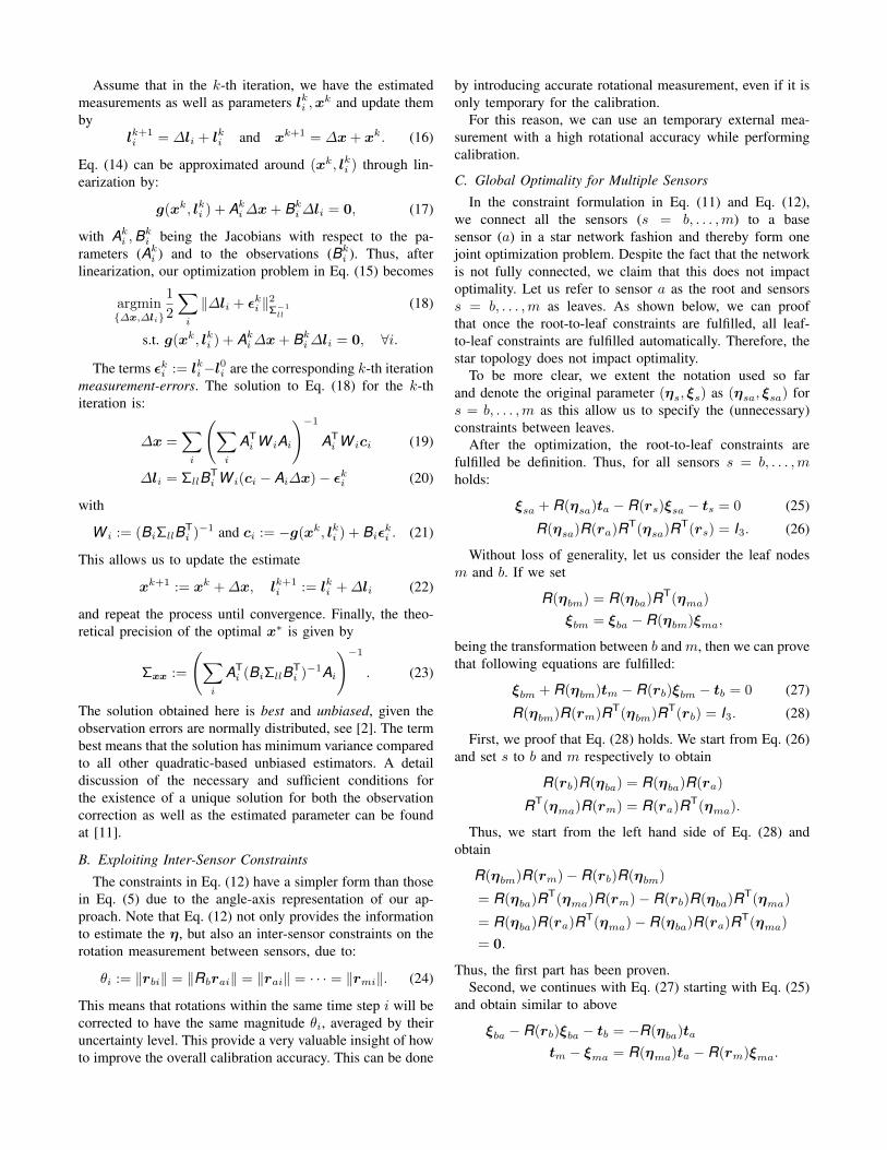
Fig. 2: Examples stereo images pairs used for calibration.

We start from the left hand side of Eq. (27) and expand ξbm,which leads toξbm − R(rb)ξbm + R(ηbm)tm − tb= [ξba − R(ηbm)ξma] + R(ηbm)tm − R(rb)[ξba − R(ηbm)ξma]− tb= [ξba − R(rb)ξba − tb] + R(ηbm)[tm − ξma] + R(rb)R(ηbm)ξma

= −R(ηba)ta + R(ηbm)[R(ηma)ta − R(rm)ξma] + R(rb)R(ηbm)ξma

= [R(rb)R(ηbm)− R(ηbm)R(rm)]ξma

= 0.

Thus, the second part has been proved. As a result, the ful-fillment of the root-to-leaf constraints automatically satisfiesall leaf-to-leaf constraints and thus they do not need to bemodeled explicitly and thus the star topology does not impactoptimality.

VI. EXPERIMENTAL RESULTS

The experiments are designed to show the capabilities ofour method and to support our key claims. We claim that ourapproach (i) accurately determines the extrinsic calibrationparameters, (ii) requires an initial guess with a level ofaccuracy that can be provided by a direct method, (iii) obtainsmore accurate results compared to ordinary least squaresusing the Gauss-Markov model, and (iv) can be executedin a reasonable amount of time to be useful for real worldapplications. We perform the evaluations on own real-worldas well as simulated datasets to support these claims.

A. Real World and Simulated Data

To evaluate our approach, we use simulated as well as realworld data. For the real world setup, we use a UAV with twostereo camera pairs (called A and B later on), one pointingforward and one pointing backwards. Example images of thiscalibration data can be found in Fig. 2. In addition to that,we place markers of a motion capture studio on the UAV tosimulate an additional sensor that has be calibrated.

In the experiment, we recorded a total of N = 1655relative motion-segments estimated through our own visualodometry pipeline [12]. Around 25 of the segments areoutliers as the visual odometry lost track. The maximumrotation angle of the inlier data is 7.6◦ and the data isrecorded at 20 fps. Fig. 3 depicts a histogram of the rotationangle and translation magnitude of the gathered data.

Fig. 3: Histogram of the rotation and translation magnitude of ourreal world dataset. Left column shows the rotation (‖r‖, in degree),and right column shows the translation (‖t‖, in meters). From topto bottom, each rows represent stereo pair A, pair B and the motioncapture studio respectively.

TABLE I: Standard deviation of the measurement noise

σr [◦] σt [mm]Stereo pair A 0.0286 2Stereo pair B 0.0286 3

Mocap 0.573 0.2

We first obtain an initial guess by the SVD-based di-rect method (e.g, [7]) then run our approach to obtain animproved solution as well as the corresponding theoreticalprecision. The covariance matrices are heuristically set toΣrr = σrI3 and Σtt = σtI3 with σr, σt given in Tab. I.We also assume the noise are independent and identicallydistributed random variables.

B. Accuracy Comparison

The first set of experiments is designed to show thatour approach computes the calibration parameters moreaccurately than an SVD-based solution and than a typicalleast squares solution based on the Gauss-Markov model.

We first performed the calibration on the real world data,and our GH approach converged at the 4th iterations. Thetheoretical precision given by our approach is depicted inTab. II. They are the square roots of the main diagonal ofthe covariance matrix in Eq. (23).

As this is a real world experiment, the ground truth is un-fortunately not available, so we cannot make an ground truthcomparison. But judging from the measurement-residualdistribution (shown in Fig. 4) given by our model after theestimation, it is clear that i) the Gaussian noise assumptionholds for our dataset to larger extent, ii) our constraint modelis correct and there is no bias in the estimation, otherwisethe residual histograms will not be symmetrically centeredaround zero. Therefore we have a good reason to believe thatthe theoretical precision given by our approach is plausible.To provide a more quantitative experiments, we performed

Fig. 4: Distribution of measurement-residuals ε after the refinementby our approach. Columns from left to right are for stereo A, B andMocap respectively. Rows from top to bottom are the 6 measure-ment components, namely r1, r2, r3 for rotation and t1, t2, t3 fortranslation. It is clear that the Gaussian noise assumption holds forour real world dataset to a large extent, and our constraint modelis correct since there is no bias.

the analysis of the accuracy in simulation, which is thesecond experiment.

In the simulation we generated in total 30,000 experiments(1000 per noise level), with noise levels starting with thevalues shown in Tab. I and scaled them with a factor varyingfrom 1 to 30. With a factor of 30, the rotation error of themotion measurement can be as much as ±25◦ according tothe 3σ principle, which is quite high compared to real motionsensors.

The methods we compared are: (i) the SVD-based directsolution (called SVD), (ii) least squares estimator basedthe Gauss-Markov model (called GM), and (iii) our Gauss-Helmert based approach (called GH). Both GH and GMare using Eq. (11) and Eq. (12) as constraint functions(or residual vectors). The initial guess to GH and GM areperturbed ground-truth values by uniform additive noise. Forreasons of comparison, we also provided a ground truthinitialization. The metric for comparison is the averagedRoot-Mean-Square-Error (RMSE) of the estimated 6 rotationparameters and 6 translation parameters from 1,000 trials.

The result of the simulation is depicted in Fig. 5. Fromthis plot, we can draw several conclusions. First, the GH andGM perform always better than SVD. The only advantage ofthe SVD is that it is a direct solution and requires no initial

TABLE II: Precision of the estimated parameters ξ,η

σξ1 σξ2 σξ3 ση1ση2

ση3

Stereo B 2.8 mm 1.90 mm 2.8 mm 0.041◦ 0.032◦ 0.033◦

Mocap 1.43 mm 1.97 mm 1.13 mm 0.165◦ 0.191◦ 0.202◦

0 10 20 30

0.00

0.05

0.10

0.15

factor

Ave

rage

RM

SE[m

]

translationSVD (direct)

GM (noisy init)GH (noisy init)GH (GT init)

0 10 20 30

0.00

0.05

0.10

0.15

factor

Ave

rage

RM

SE[r

adia

n]

rotationSVD (direct)

GM (noisy init)GH (noisy init)GH (GT init)

Fig. 5: Accuracy comparison through Monte-Carlo simulation. Thex-axis show the factor by which we scale the input noise forthe translational (left) and rotational (right) component. The plotsshow the RMSE for the direct SVD approach, the GM as well asGH model using a noisy initialization, and finally the GH modelinitialized with the ground truth as the initial guess. The GHmodel outperforms the other approaches as expected and performsidentical if initialized with noisy values or the ground truth ones.

guess. Second, the GH and GM approaches produce identicalresults as long as the noise-level is small. Third, as the noiselevel increases, the accuracy of the GM solution degradeswhile our GH solution does not. The error of the GH solutiongrows linearly with the increased input noise, which is theexpected theoretical result. Thus, we can conclude that overthe spectrum of all situations, our GH approach performsbest. At the highest noise-levels, GH is better than GMby 75% in translation (0.0287 vs. 0.1150), and by 71% inrotation (0.0095 vs. 0.0314) in this simulation setup. Onlyfor situation with low noise (eg, a factor smaller than three),GH and GM show the same performance as can be expectedgiven our explanation in Sec. IV. Finally, we can see thatthe GH approach produces the same results if using the GTfor initialization or a noisy variant of it.

C. Robustness with Respect to the Initial Guess

This experiment is designed to show that our approach isrobust enough to use an initial values from a direct approachIn the previous experiments, we compared a ground truthinitialization to perturbed values for the sake of comparison.But in reality, however, we have to obtain the initial guesseither by manual measure or by utilizing a direct approach. Inthis experiment, we perform a similar experiment as beforebut with the initial guess coming from the SVD method,i.e. without any knowledge about the true configuration. Wecompare these to the results, which are obtained when usingthe ground truth as the initial guess. The results are depictedin Fig. 6 and show that the RMSE curves are identical forboth initializations, hence we conclude that our approachis robust enough to be used in combination with SVD forproviding the start value for the optimization.

D. Runtime

The last set of experiments in designed to illustrate thecomputation requirements of our approach and to show that

0 10 20 30

0.00

2.00

4.00

·10−2

factor

Ave

rage

RM

SE[m

]translation

GH (GT init)GH (SVD init)

0 10 20 30

0.00

2.00

4.00

·10−2

factor

Ave

rage

RM

SE[r

adia

n]

rotationGH (GT init)

GH (SVD init)

Fig. 6: Accuracy in relation to the initial guess for different noiselevels on the translational and roitational component. In all cases,the initialized via the SVD result or with the ground truth producesthe same results. Thus, we conclude that we can safely use SVDto initialize our GH optimization.

real world calibration can be done easily. For our real worldcalibration, we considered 1,630 poses extracted from eachof the three sensors. The timings of our Python code runningon a i5 notebook computer are approx. 6 s for the overallapproach. Around 600 ms is used for computing the initialsolution using SVD and around 1.2 s-1.5 s is required periteration. These timing involves all computations, except themotion estimation from the sensors itself, in this case thevisual odometry. At least in our setup, computing the visualodometry takes longer than the calibration itself.

E. Summary

In summary, our real world and simulation experimentssuggest that our Gauss-Helmert based calibration approachoutperforms the direct SVD-based approach as well as theordinary least squares solution that is based on the Gauss-Markov model. The use of the Gauss-Helmert model withconstraints allows us to provide better results than all otherapproach at high noise levels and produces the identicalresult than the Gauss-Markov model for small noise levels.We furthermore showed that our approach is robust enoughwith respect to the initial guess provided by the direct SVDapproach. In real world settings, the optimization is fasterthan the time needed to compute a visual odometry and werequired 6 s in a i5 notebook to calibrate 3 sensors with1,630 poses each. Thus, we supported our claims with thisexperimental evaluation.

VII. CONCLUSION

In this paper, we presented a novel approach to computethe extrinsic parameters of multiple sensors installed on amoving platform. Our approach defines constraints betweenthe motions of the individual sensors given that they arerigidly mounted in the robot and then computes the extrinsicparameters in a statistically sound way using the Gauss-Helmert model. This allows us to successfully determine therelative transformations between the origins of the sensorcoordinate systems as the robot’s base. We implemented andevaluated our approach in simulations as well as on real data.The experiments suggest that our approach can accuratelydetermine the extrinsic parameters of the individual sensorsunder realistic conditions. We provided comparisons to a

direct SVD approach as well as to the ordinary Gauss-Markov least squares estimation and furthermore supportedall claims made in this paper through our evaluation.

REFERENCES

[1] S. Agarwal, K. Mierle, and Others. Ceres solver. http://ceres-solver.org.

[2] A. R. Amiri-Simkooei. Least-squares variance component estimation:theory and gps applications. 2007.

[3] Y. Chang, X. Lebegue, and J. K. Aggarwal. Calibrating a mobilecamera’s parameters. Pattern Recognition, 26(1):75–88, 1993.

[4] K. Daniilidis. Hand-eye calibration using dual quaternions. TheInternational Journal of Robotics Research, 18(3):286–298, 1999.

[5] F. Dornaika and R. Horaud. Simultaneous robot-world and hand-eye calibration. IEEE transactions on Robotics and Automation,14(4):617–622, 1998.

[6] W. Forstner and B. P. Wrobel. Photogrammetric Computer Vision.Springer, 2016.

[7] C. X. Guo, F. M. Mirzaei, and S. I. Roumeliotis. An analytical least-squares solution to the odometer-camera extrinsic calibration problem.In Proc. of the IEEE Int. Conf. on Robotics & Automation (ICRA),2012.

[8] L. Heng, B. Li, and M. Pollefeys. Camodocal: Automatic intrinsicand extrinsic calibration of a rig with multiple generic cameras andodometry. In Proc. of the IEEE/RSJ Int. Conf. on Intelligent Robotsand Systems (IROS), 2013.

[9] R. Kummerle, G. Grisetti, and W. Burgard. Simultaneous calibration,localization, and mapping. In Proc. of the IEEE/RSJ Int. Conf. onIntelligent Robots and Systems (IROS), pages 3716–3721, 2011.

[10] R. Kummerle, G. Grisetti, H. Strasdat, K. Konolige, and W. Burgard.g2o: A general framework for graph optimization. In Proc. of theIEEE Int. Conf. on Robotics & Automation (ICRA), pages 3607–3613,2011.

[11] F. Neitzel and B. Schaffrin. On the gauss–helmert model with asingular dispersion matrix where bq is of smaller rank than b. Journalof computational and applied mathematics, 291:458–467, 2016.

[12] J. Schneider, C. Eling, L. Klingbeil, H. Kuhlmann, W. Forstner, andC. Stachniss. Fast and effective online pose estimation and mappingfor uavs. In Proc. of the IEEE Int. Conf. on Robotics & Automation(ICRA), pages 4784–4791, 2016.

[13] S. Schneider, T. Luettel, and H. Wuensche. Odometry-based onlineextrinsic sensor calibration. In Proc. of the IEEE/RSJ Int. Conf. onIntelligent Robots and Systems (IROS), pages 1287–1292, 2013.

[14] Y. C. Shiu and S. Ahmad. Calibration of wrist-mounted robotic sensorsby solving homogeneous transform equations of the form ax=xb. IEEETran. on Rob. and Aut., 5(1):16–29, Feb 1989.

[15] K. H. Strobl and G. Hirzinger. Optimal hand-eye calibration. InProc. of the IEEE/RSJ Int. Conf. on Intelligent Robots and Systems(IROS), 2006.

[16] Z. Taylor and J. Nieto. Motion-based calibration of multimodal sensorarrays. In Proc. of the IEEE Int. Conf. on Robotics & Automation(ICRA), pages 4843–4850, 2015.

[17] R. Y. Tsai and R. K. Lenz. Real time versatile robotics hand/eyecalibration using 3d machine vision. In Proc. of the IEEE Int. Conf. onRobotics & Automation (ICRA), 1988.

[18] H. Wolf. Das geodatische Gauß-Helmert-Modell und seine Eigen-schaften. pages 103:41–43, 1978.

[19] Z. Zhao. Hand-eye calibration using convex optimization. In Proc. ofthe IEEE Int. Conf. on Robotics & Automation (ICRA), pages 2947–2952, 2011.