3 NQ(

SYMPLECTIC INTEGRATION OF NONSEPARABLE

HAMILTONIAN SYSTEMS

THESIS

Presented to the Graduate Council of the

University of North Texas in Partial

Fulfillment of the Requirements

For the Degree of

MASTER OF SCIENCE

By

David M. Curry, B.S.

Denton, Texas

May, 1996

3 NQ(

SYMPLECTIC INTEGRATION OF NONSEPARABLE

HAMILTONIAN SYSTEMS

THESIS

Presented to the Graduate Council of the

University of North Texas in Partial

Fulfillment of the Requirements

For the Degree of

MASTER OF SCIENCE

By

David M. Curry, B.S.

Denton, Texas

May, 1996

Curry, David M., Symplectic integration of nonseparablp Hamiltnnian

systems. Master of Science (Computer Science), May, 1996, 51 pp., 2 tables, 2

figures, references, 13 titles.

Numerical methods are usually necessary in solving Hamiltonian systems

since there is often no closed-form solution. By utilizing a general property of

Hamiltonians, namely the symplectic property, all of the qualities of the system

may be preserved for indefinitely long integration times because all of the inte-

gral (Poincare) invariants are conserved. This allows for more reliable results and

frequently leads to significantly shorter execution times as compared to conven-

tional methods. The resonant triad Hamiltonian with one degree of freedom will

be focused upon for most of the numerical tests because of its difficult nature and,

moreover, analytical results exist whereby useful comparisons can be made.

ACKNOWLEDGEMENTS

This research was funded by the Office of Naval Research (ONR) under

grant #73191.

This thesis was typeset by the TgX macro system of the

American Mathematical Society.

TABLE OF CONTENTS

List of Tables v

List of Figures vi

Chapter I. Introduction 1

§1.1. Hamiltonians

§1.2. Numerical integrators

§1.3. Symplectic integrators

§1.4. The resonant triad Hamiltonian

Chapter II. A Symplectic Integrator 6

§2.1. Runge-Kutta methods

§2.2. Symplectic Runge-Kutta conditions

§2.3. A symplectic Runge-Kutta scheme

§2.4. Implementation of symplectic scheme

Chapter III. Results and Conclusions 19

§3.1. Accuracy

§3.2. Comparisons

§3.3. Conclusions

Appendix A. Symplectic Properties 23

Appendix B. Numerical Programming Nuances 26

Appendix C. Source Code (Fortran 90) 30

References 50

LIST OF TABLES

Table 1. Conventional vs. symplectic methods 20

Table 2. Different symplectic implementations 21

LIST OF FIGURES

Figure 1.1. Resonant triad 5

Figure B.l. Henon-Heiles system 28

CHAPTER I

INTRODUCTION

1.1. Hamiltonians

In physics, modeling phenomena by means of Hamilton's formalism is a

powerful and often used tool. Application of this formalism yields the Hamil-

tonian of the system (phenomena). More precisely, a Hamiltonian is an equation

which, when derived for a particular system, expresses the dynamics of that sys-

tem by means of a system of first-order differential equations appropriately re-

ferred to as Hamilton's equations of motion. Specifically, Hamilton's equations of

motion constitute a system of 2N first-order differential equations such that

. dH Qi =

dpi

dH » = 1 , . . . , J V , (1.1)

Ft ~ a oqi

where H is the Hamiltonian, q = (</i, • • • > QN) is the generalized coordinate vec-

tor, p = • • • ,Pn) is the canonical momentum vector conjugate to the gener-

alized coordinate vector, and N is the number of degrees of freedom in which the

system acts.

Due to the general nature of a Hamiltonian system, it is not realistic to as-

sume that the system is well-behaved or even integrable. Numerical integration is

therefore key in understanding the dynamics of many Hamiltonian systems which

may be deemed chaotic or stable for various trajectories based solely upon the

information provided by the numerical method chosen. Although Hamiltonian sys-

tems are quite general, there is one particular property of importance: Hamilto-

nians are symplectic. The term symplectic comes from the Greek word meaning

"intertwined" and refers to the special interdependence of the canonical variables

q and p. This interdependence is the symplectic property and is written

• i d H n ^ V = 3 W (1-2)

where (

77 = I I and V P / (1.3) -a::

The symplectic property is important because if a Hamiltonian is acted upon by

a transformation which preserves the symplectic property, then the transformed

Hamiltonian also preserves every other quality of the original Hamiltonian [1].

1.2. Numerical Integrators

Since an accurate model of a physical system often requires an accurate

solution to Hamilton's equations of motion, precise numerical integration meth-

ods are quite important. Standard numerical integrators cannot, by their gen-

eral nature, make assumptions about any natural symmetries within a system of

equations to be integrated. For this reason, the error incurred through numerical

integration is distributed, for all practical purposes, randomly about the actual

solution and accrues as we integrate further from the initial point. If this error is

large enough, it may create the impression of chaos when there is none, destroy

KAM tori or, if periodic or quasi-periodic orbits exist, closed orbits may appear

open. While it is true that smaller time-step sizes reduce the error (usually), this

is not effective for long-term integration for two reasons:

1. The time-step size required may be so small that internal calculations

may exceed machine limits and

2. There will always exist a certain lack of certainty in the results, be-

cause there is no guarantee that the chosen time-step is small enough

to accurately reflect the system's qualities.

Hence, there is a strong need for a specialized integrator—a symplectic integrator.

1.3. Symplectic Integrators

A symplectic integrator conserves the phase flow or, more exactly, the

Poincare (integral) invariants of the Hamiltonian system. For this reason, sym-

plectic integrators are ideally suited for integrating Hamiltonian systems over long

periods of time since they preserve these qualities globally, whereas other schemes

cannot. There are many integration schemes which may be constructed so that

they are symplectic. Most of them, however, are only symplectic for separable

Hamiltonians, i.e. Hamiltonians for which the potential depends only upon the

generalized coordinates. However, many Hamiltonians are nonseparable.

The resonant triad Hamiltonian is an example of a nonseparable Hamilton-

ian and so is the Henon-Heiles Hamiltonian. The Henon-Heiles system is a classic

test of integrators which handle the nonseparable case, but I will present it only

for comparison purposes with other symplectic methods developed elsewhere. The

significance of the Henon-Heiles Hamiltonian lies in astrophysics. The Henon-

Heiles Hamiltonian is written

H = 2 ^ 1 ~^~P2 ^2) + Q1Q2 — g #2- (1-4)

However, the integration of the resonant triad Hamiltonian system will be para-

mount as it is a more strenuous test for an integrator. Whereas the Henon-Heiles

system is nonstiff, the resonant triad system is stiff. In practice, a stiff equation is

one in which the variables vary by different time-scales from one another.

1.4. The resonant triad Hamiltonian

Because the symplectic integrator will be developed with the resonant triad

(and all systems like it) in mind, a brief description of this Hamiltonian is in or-

der. The resonant triad Hamiltonian describes a physical system of three waves

interacting where nonlinear terms arise from weak anharmonicities [10]. One

such set of waves are a triad of three short gravity-capillary water waves travel-

ing along a much longer gravity wave so that

H = HO — 7 j cos ut (1.5)

and

Ho = \ / j ( l - j ) ( j + j*)smi>, ( 1 . 6 )

where j is the wave action and is the canonically conjugate phase [11,12]. At

high energies, Ho is smoothly varying; however at low energies, it is not (see Fig-

ure 1). This creates a conditions under which we may test the ability of the in-

tegrator to handle discontinuous (or nearly so) first derivatives. HQ is what is

known as the unperturbed Hamiltonian. The other term in H is the perturbation.

7 is the strength of the perturbation and to is its frequency. The exact solution of

the wave number, j , for the unperturbed case (7 = 0), is

j ( t ) = h ~ C?3 - 32) sn2 TiVh ~ j i ( t - t 0 ) (1.7)

where ji, j'2, and jz are the roots of the equation j2( 1 - j) = E2 ordered so that

j i < J2 < jz, E represents the energy of the unperturbed system, and sn is the

FIGURE 1. The resonant triad Hamiltonian: a) in the high-energy regime where j and tp are very smooth ( j is the dashed line) and b) when the energy is low, where j and ip develop discontinuities in their first derivatives.

Jacobi sine function [13]. The solution therefore involves an incomplete elliptic

integral of the first kind since

snu = sin /" Jo

dB (1.8)

y/l — k2 sin2 9

where A; is a constant. Although this does not have an exact solution itself for

arbitrary values of u, it is a periodic function with periods of AK and 2 iK' , where

K j-n/2

Jo

dB

\ / l - k2 s i n V

fw/2 j f - /

^0

dd

\ / l — k'2 sin2 6 (1.9)

and k' = \ / l - k2. From this, it is possible to measure the global error of the the

integrator by comparing values periodically.

CHAPTER II

THE SYMPLECTIC INTEGRATOR

2.1. Runge-Kutta Methods

Runge-Kutta methods are a common, probably even the most common,

method for numerical integration. The idea is to approximate at time t + h, where

h is referred to as the step-size, the value of a differential equation for which the

value is known at time t. Then the value at time t + nh is approximated from the

one at time t + (n — l)h ad infinitum. The error incurred in taking each individ-

ual time-step is called the local discretization error whereas the error accumulated

over the entire span of the integration is the global discretization error. There are

many different Runge-Kutta schemes because the constraints on the free param-

eters do not lead to a unique solution. In general, given a system of differential

equations

f = r ( y ,t). (2.1)

where y, F € M.N and t € R, an s-stage Runge-Kutta method is defined by the

system

yn = y (*»),

hn = tn+1 ~ tni

S

« = (2.2) S

a ='

j=i

— y + hn ^ ^ (ijjF(Yj, tn -h c^/in) (2-3) j=i

and S

yn+1 =yn + h^biFiYi.tn + Cihn) + 0 ( ^ + 1 ) , (2.4) i=1

where r is the order of the method (r + 1 is the order of the local discretization

error) and s is the number of stages. The bi are referred to as the weights of the

system, the q are the abscissae, and the Yj are the internal stages. It is standard

to write the parameters in the form of a tableau as follows:

ail • • * o-i s

a, ... a • <2'5' ^sl ^ss

\h ••• bs

Once the above tableau is fixed, the Runge-Kutta method is uniquely determined.

It is important to note that if a^- = 0 whenever i < j, the method is explicit;

otherwise it is implicit.

2.2. Symplectic Runge-Kutta Conditions

In order to derive the conditions that a Runge-Kutta method be symplectic,

we will use a proof similar to one given by Sanz-Serna [6], but we will use Pois-

son brackets rather than differential forms. The Poisson bracket, [ f ,g] q , p , of two

functions f(q,p) and g(q,p), where q,p € and / , g : H2N i-* R, is

[ / ,* ]„ ,= ( V/, J V*), (2.6)

where (u, v) is the inner product of u and v and J is

J s ( i o ) ' (27)

where 0 is the N x N zero matrix and I is the N x N identity matrix.

8

Poisson brackets may be extended to vector-valued functions f, g : R2N i-»

by defining the square-matrix Poisson bracket

^ [fli9l]q,p [fNi9l]q,p ^

: ; , (2.8)

\ [ / l i 9N]q,p • • • [In, 9N]q,p J

where f, g are functions of q and p, where q, p G K . For convenience, we will

denote the Poisson bracket by a wedge, A, so that

f A g = [f,g]„,P. (2.9)

The wedge product (Poisson bracket) is both bilinear, meaning that

(ccf + g) Ah = a f A h + /?gAh (2.10)

and antisymmetric, so that

which implies that

Equation (2.11) follows from

f A g = - g A f

f Af = 0.

(2.11)

(2.12)

/Ap=(V/ , JV<7)

M ( .

J p j V I 0

k f p J \ 9q

= (fp->9q) ~~

9q

<9p.

(2.13)

where

fa —

/ \ dqi \

jQJ— dqN '

(2.14)

and fp, Qq. and ()p are defined in like manner. A third property of the wedge

product is that the sum of the cyclic permutations of the wedge product of f, g,

and h is zero, i.e.

(f A g) A h + (g A h) A f + (h A f ) A g = 0. (2.15)

These properties show that the wedge product constitutes a Lie algebra.

This is a convenient way to check whether a transformation is symplectic

because it can be shown that if 0 is a transformation such that (q*,p*) = 0(q, p),

then 0 is a symplectic transformation if, and only if,

dq* A dp* = dq A dp. (2.16)

Applying equations (2.3) and (2.4) to a Hamiltonian system, a Runge-Kutta

method defines a transformation ^ such that (q n + 1 ,p n + 1 ) = 3>(qn, pn) where

Q = Q + hn ftjf(Qj, Pj, tn + Cjhn), i=l

s

Pn+1 = Pn + K biS(Qi, Pi, tn + Cihn), i=l

s

Qi — q + hn a^f(Qj, Pj,tn + Cjhn),

Pi P + hn ^ Pj? tn + Cjhn), 3 = 1

(2.17)

(2.18)

(2.19)

(2.20)

for f(q, p,£) — dH/dp and g(q, p, t) — —dH/dq. We seek conditions on ^ such

that dqn+1 Adpn + 1 = dqnAdpn, i.e. is symplectic. Therefore, let us begin with

10

equations (2.17) and (2.18) and differentiate them to produce

S

dqn+1 A dpn+1 = dqn A dpn + hn M f (Qi, Pi, tn + Cihn) A dpn

i=l s

+ h n ^ 2 fydq™ A dg(Qj, P j,tn + Cjhn) j = 1

S

^ ] bibjdf(Qi, Pj, -f- Cj/in) A rfg(Qj) ~f~ Cjhn) i,j=i

(2.21)

From this last equation, it is quite clear that \I> is symplectic (dqn+1 A dp n + 1 =

dqn A <ipn) if the condition

hn hdf(Qi, Pi, tn + Cihn) A dpn + hn bjdqn A dg(Qj, Pj, tn + Cjhn) i=1 j=l

s

^ y bibjdf(Qi, P j , tn + Cihn) A d g ( Q j , P^ , f n + Cjhn) = 0

(2.22)

is met. By differentiating equations (2.19) and (2.20) and solving for q n and p n ,

equation (2.22) may be rewritten

hn ^ h [df(Qi, P , , tn + Cihn) A dPi + dQi A dg(Qi, P j , tn + Cihn)] i=1

s

~ + bjdji — bibj)df(Qi, P j , tn + Cihn) A rfg(Qj, Pj,tn + Cjhn) = 0 i j= l

(2.23)

We will show that for each i in the first summation, the expression vanishes by

exploiting the properties of a Lie algebra. Consider that, for each i, we can sepa-

rate the N-vectors (where N is the number of degrees of freedom) into their con-

11

stituent variables, so

N

dV A <(Q, + dPi A dg< = £ ( # < A dQi + dP; A dgi)

n=l

N ( d P d f i

= E H,v=l \ ^

dgl + _ | d p . A ( i Q l + _ & d p . A ^

^ / Q t f j i P&T-fi

= £ J ^ Q i A i Q » + a ^ d P " A d Q

d2Hi d2Hi

-dPl A dQl - ^ r ^ d P l A dPl m " d p v d p ~ ~ v ^ u

JL ( Q 2 f j i f)2 f f i \

= £ J ^ Q i A d Q > - ^ d P i A d P i )

= 0 (by antisymmetry), (2.24)

where we have employed the notation that f* = f(Qj, P i 5 tn + Cihn) and gi =

g(Qi, Pi) in + Cihn). This can also be shown without the use of differential forms

by using Jacobians instead [5]. Because the first summation vanishes, the sec-

ond summation in equation (2.23) vanishing is the only condition left to be met

so that ^ is symplectic. Therefore

biQij -f- bjdji bibj — 0, i, j ' — 1 , . . . , s (2.25)

is a sufficient condition which guarantees that ^ is a symplectic transformation.

2.3. A Symplectic Runge-Kutta Scheme

The particular scheme which we will employ is called a Gauss method.

Gauss methods are collocation methods, which means that they are based upon

12

building an interpolating polynomial such that

un(tn) = yn and (2.26)

Un( n "I" Cihn) ~ "I" Ci n)>^n i 1 . . . S,

(2.27)

so that

yn + i = un (tn+i) (2.28)

where un is the interpolating polynomial from time tn to tn+1. The connection is

that un defines a Runge-Kutta Method where

Yj = u n ( t n + Cihn) and (2.29)

F(Yj, tfi -f~ Cj/lyj) — Un( n ^i^n)) i —— 1, . . . , S. (2.30)

Now, we must integrate the un to find un. We will employ a weighted sum quad-

rature rule, so that

ftn-f-1 u n(t)dt =

i=l

which can be transformed to

rtn+1 / Un(t)dt = 22 biUn(tn + CiK) + 0 ( ^ + 1 ) (2.31)

J tr> ' 1

[ <f>(t)dt = J2 J° i=i

buKci) + O (hrn

+1) (2.32)

by taking u^(t + tn/hn) t-» <f)(t) to simplify the algebra. In order to achieve a

method of order r = 2s (local error of order 2s + 1), equation (2.32) must be exact

for polynomials of degree < 2s — 1.

We can now derive the tableaus for symplectic Runge-Kutta methods of ar-

bitrary order. We are only concerned here with the relatively lower orders of two

(s = 1) and four (s = 2) for our algorithm. Therefore we will derive both of them

13

starting with the second-order method. Because equation (2.32) must be exact for

polynomials of degree < 2s — 1 in order for the method to have order 2s, we have

the following restraints when s = 1:

= 1 => f (j>(t)dt = b\(j>{c\) = 1 and Jo 1 f1

(j){t) = (*--)=• J (f){t)dt = bi<f>(ci) = 0,

(2.33)

where t — 1/2 was chosen because of symmetry (1/2 is the midpoint). Prom this

system, it is easy to see that

&i = 1 and

x j (2.34)

h(ci - j ) = 0 =>• ci = -

and from equation (2.2) we find that

ail = Ci = - . (2.35)

Now, we have uniquely defined the tableau so we must check if this result is sym-

plectic. Prom equation (2.25), the symplectic condition with s = 1 becomes

2Mn - b\ = 0 (2.36)

and this indeed checks out. Therefore, the tableau for our second-order symplectic

Runge-Kutta scheme is

I a n I \ — = - . (2.37)

\bi |1

The fourth-order method can be derived in the same spirit. With s = 2, we

14

get the following four conditions:

(f){t) = l=> f <f>(t)dt = &i^(ci) + b2(f)(c2) = 1, Jo

1 f1 (j)(t) = (t - - ) =» J <j)(t)dt = bi</>(ci) + b2<j)(c2) = 0,

<j>(t) = (t - ^)2 =>• J <j){t)dt = M ( c i ) + b2<f>(c2) = and

1 Z"1

4>{t) = (t - -^)3 =* j <l>(t)dt = bi(j)(d) + 620(c2) = 0.

This implies the following nonlinear system of equations:

(2.38)

b\ + b2 — 15

h(ci - - ) + b2(c2 - - ) = 0,

h(ci - -)2 + b2(c2 - - ) 2 = — , and

1, , . . , 1.

(2.39)

h(ci - ^)3 + b2(c2- - ) 3 = 0.

Fortunately, this has a real solutions in the interval [0,1] for each variable [7]. The

solution is

h = h = \ (3.40)

1 V3 l x / 3 , C l ~ 2 6 ' C 2 ~ 2 + 6 ' ^3'41^

Examining equation (2.2) with s = 2 we see that the c's do not uniquely define the

o's. But using the symplectic condition (2.25), we have

an + ai2 = ci,

a2i + o22 = c2,

2on - 6i = 0, (3.42)

feiai2 + b2a21 — fei&2 = 0, and

2<l22 — b2 = 0

15

which has the unique solution (only four of these equations are linearly indepen-

dent)

a n = - °i2 - 4

_ 1 x/3 a21 — 7 H 77~

4 6

1 \/3 T

l ' a 2 2 = 4

(2.43)

We now have uniquely defined the tableau for a fourth-order symplectic Runge-

Kutta method which is

a n o, 12

a2i 022 —

l 4

I + 4 6

1 4

v l 6

b\ 62

(2.44)

2.4. Implementation of Symplectic Scheme

Because the second-order and fourth-order methods derived above are both

implicit methods, it is necessary to decide upon a tactic by which the computer

can solve them efficiently. There are two common approaches: fixed-point iter-

ation and Newton's method. Newton's method, which is based upon Jacobians,

generally exhibits much faster convergence but is more expensive to compute

at each iteration. Fixed-point iteration, on the other hand, is relatively cheap

to compute at each iteration, but usually requires many more iterations. Hamil-

tonian equations have been observed to usually converge in less time using fixed-

point iteration rather than using Newton's method. Therefore it is better to utilize

fixed-point iteration for these equations even though Newton's method is, in other

cases, usually superior. Implementing fixed-point iteration is straight-forward.

Let designate the uth iteration of Yj, then iterate

a

Yj"+1) = y„ + J2 OijFtYl"1, („ + c,h„) (2.45)

Y^+i] _ • i

y M 1 i

vM i

16

until Y^+i] _

< e, (2.46)

where e is the desired relative tolerance. We can then take Yj = Y ^ + 1 \ To

chose the value of Y?0-' to begin the iterations, three approaches may be em-

ployed. The first approach is to choose y]0^ = yn . This is computationally

cheap but may not be a good choice. Another approach is to take y[0^ = Yj,

where is the value from the previous time-step. This is equally cheap and

is a good choice, especially when hn is small. Lastly, we can extrapolate y|°^

from an interpolating polynomial of some degree d which interpolates the points

(y(n d^tn-d)i (Y | n - d + 1 \ t n -d+i ) , • • •) (Y^n\tn), where the superscript (n) in

Y ^ refers to the value of Yj at time tn. Often, it is not a good idea to use an

interpolating polynomial of degree greater than two because the higher order

terms have such large moments. Considering the quick convergence of a Hamil-

tonian system, the second approach is most likely to be the fastest one overall.

Finally, some method of deciding the step-size must be chosen. A fixed

step-size is one alternative, where the step-size is set at the start of the integra-

tion and never varied. This is sometimes preferable for nonstiff problems, but for

stiff problems it is better to allow the step-size to vary so that in slowly changing

regions the step-size will be large and in quickly changing regions the step-size will

be small. When choosing a step-size for a fixed step-size method, the step-size, h,

must meet the requirement

h < (2.47)

where

L = min j l / € R : L ' > ~ ^ V u , v | (2.48)

17

is the Lipschitz constant in order to ensure convergence.

Variable step methods are much more involved. One method which may be

employed for both the second-order and the fourth-order schemes is to take a step

from time tn at some tentative step-size hn and also, from time £n, take two steps

of size hn/ 2. Let us take the solution taken with step-size hn and call it y^t+1 and

that taken with two steps each of size hn/2 and designate it y^+1. One simple

method would be to bisect h (hn+1 —> hn/2) whenever

lly«+i -yn+ill > e (2-49)

and to double hn (hn+i —> 2hn) if, on the first iteration,

l|y»+i-y»+ill < c - (2-5°)

This method will be referred to as the bisection method. This simple strategy

may by improved upon theoretically by using the value of err, where err =

l|y«+i - y«+iII• hn+1 may be taken to be

[ Sh™ li??|1/(r+1) ' e > e r r

hn+l=< (2.51) I S h n I if? I ' e < err

where r is the order of the method and S is a safety factor (usually taken to be

0.8) [9]. This method will be called the modified bisection method.

A final method is the method of differing orders [8]. Because this scheme

requires the use of a lower-order method, it cannot be used with the second-order

method. Here we will change our notation slightly so that the solution taken with

the second-order method will be called y^+1 and that taken with the fourth-order

method will be designated y^+1. Both orders take a step of size hn. The next

step size will be taken as

€ \l/(r'+l) h, n + l

/ e \ w - hn ( — J , (2.52)

18

where r' is the order of the lower-order method. This is because err is of order r'

since y'n is of order r'. Hence, in this case,

/ e \V3

hn+1 = K ( - ) . (2.53)

All of these methods for determining the step-size are compared to one another in

the next chapter using the resonant-triad interaction Hamiltonian.

CHAPTER III

RESULTS AND CONCLUSIONS

3.1. Accuracy

Accuracy is an important issue when discussing the merits of one numerical

method over another. But before accuracy can be compared, it is essential to un-

derstand how it can be measured. Some problems have exact solutions to which

the numerical ones may be directly compared. This is a straight-forward case and

is easy to understand. However, most problems which will be integrated will not

have an exact solution, so we need to find other methods by which to quantify

accuracy. One method stands out when dealing with conservative Hamiltonian

systems.

A conservative system is one in which the energy is constant. In a conser-

vative Hamiltonian system, energy is one of the integral (Poincare) invariants.

Hence, the change in energy of the system is a good measure of the accuracy of

the method and is the one which will be employed. All measurements are cal-

culated in terms of the relative error. One point must be made very clear: the

term accuracy is used throughout to denote the ability to conserve physical quan-

tities in a system such as energy as opposed to the common definition of accuracy

whereby accuracy refers to the order of the method.

3.2. Comparisons

Table 1 summarizes the global error (a measure of accuracy) and the ex-

1 o

Method Henon-Heiles Resonant triad

Method global err. CPU time global err. CPU time

Symplectic 1.9xl0~6 284 3 .6xl0~ 6 475

Conventional 2 .0xl0~ 5 114 6 .2xl0~ 6 206

TABLE 1. Comparison of global error and execution time (in C P U

seconds) between conventional and symplectic methods on an 83MHz Intel P 2 4 T .

20

ecution times of of both the symplectic integrator and a conventional integrator

(fourth-order Runge-Kutta with variable step-size). The global error was calcu-

lated as the relative deviation from the initial energy. As was expected, the sym-

plectic method turned out to be much more accurate, but did surprisingly poorly

when compared in terms of speed. Also, different implementations of the symplec-

tic method were compared against one another.

Four different implementations of the of the Symplectic Gauss method are

compared. One implementation uses the last solution as an initial guess for the

next step and uses the bisection method for varying the step size. Another also

uses the last solution as an initial guess for the next step but uses the method of

differing orders for varying the step size. Next, one uses quadratic extrapolation

to generate an initial guess with the bisection method for varying the step size.

And finally, the last one uses quadratic extrapolation to generate an initial guess

but uses the method of differing orders for calculating the step size. The results

are summarized in Table 2. The method of differing orders is far superior to the

bisection method, which is understandable because the bisection method cannot

vary the step size by more than a factor of two in any single iteration, whereas

the other method is not restricted. Also, choosing an initial guess by quadratic

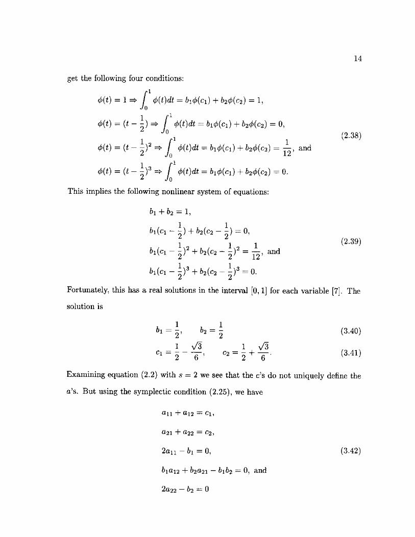
21

System

Initial guess

System use last quad. ext.

System Step size Step size

System

bisection diff. ord. bisection diff. ord.

Henon-Heiles 1531 374 1396 326

Resonant triad 2425 675 2371 497

TABLE 2. Comparison of execution time for different implementations of the symplectic method on an 83 MHz Intel P24T measured in CPU seconds.

extrapolation is superior to that of simply using the last solution. The trade-off

between the two is that quadratic extrapolation is more expensive to compute,

whereas using the last solution is cheap but results in more iterations which is

ultimately more expensive. All integrations went from t = 0 to t = 3000 with

Qi0 ~ Q20 = Pi0 = P2o = 0-12 for the Henon-Heiles system and ipo = 7r/6, jo =

0.003 for the resonant triad Hamiltonian.

3.3. Conclusions

Symplectic integration of nonseparable Hamiltonians is more accurate (in

the sense of preserving the Poincare invariants) than using traditional methods.

However, symplectic methods in this case are also markedly slower. It is worth

noting that the degree by which the accuracy increases by using symplectic inte-

gration is dependent upon the system being integrated. The resonant triad system

benefited by a two-fold increase in accuracy while the Henon-Heiles system which

is less stiff received an entire order of magnitude in increased accuracy. Because

the local discretization error in each comparison run was kept as close to identi-

cal as possible for each of the different integration schemes, any difference in the

22

error accumulated in the measured energy signifies a difference in ability to pre-

serve the conserved quantities within Hamiltonian systems. Although symplectic

methods in the case of separable Hamiltonians can be much faster as well as more

accurate than conventional methods [3], the tricks applied to obtain the speed ob-

served in the separable case cannot be applied in the nonseparable case. So while

the decision to use a symplectic integrator in the case of a separable Hamilton-

ian is obvious since these methods are usually both faster and more accurate, the

decision is not so clear when the Hamiltonian is nonseparable because now the

increased accuracy comes at the cost of decreased speed. In conclusion, we have

developed a symplectic integrator for nonseparable Hamiltonians and have found

that it is more accurate in terms of preserving Hamiltonian invariants but there is

a significant trade-off in speed.

APPENDIX A

SYMPLECTIC TRANSFORMATIONS

Definition

Taking a tack along that of Goldstein [2], a symplectic transformation is a

canonical transformation of the Hamiltonian, so let M be a canonical transforma-

tion which maps f} (->• tin), i-e.

< = M,j, (A.1)

where r) = (q, p) is the vector containing the generalized coordinates and mo-

menta for some Hamiltonian H. Since H is Hamiltonian, r) satisfies

V = ^ , (A.2)

where J is defined as the 2N x 2N matrix

J = ( - I o ) ' ( A 3 )

N being the degrees of freedom associated with the Hamiltonian H. Because M

is a canonical transformation, Hamilton's equations must, by definition, also hold

for £. Therefore,

C = (A.4)

But, there is another relation which can be derived for £. Combining Equations

(A.l) and (A.2), we can write

C = M J ^ . (A.5)

24

which then becomes ~dH

C = M J M — . (A.6)

since dH ~dH / k x

M ( A ' 7 )

which, together with Equation (A.4), implies the symplectic condition for a canon-

ical transformation, namely

M J M = J. (A.8)

Hence, any transformation which satisfies Equation (A.8) is symplectic. It is also

possible to write the symplectic condition in terms of Poisson brackets. We can

express the Poisson bracket of two functions «(q, p) and f(q, p) as

T , du dv du dv ,

[u, v]q!p = — — — (A.9) dqidpi dpidqi '

From this equation is easy to see that

\.QiiQj]q,p ~ \PiiPj\q,p = 0 (A.10)

and that

[QiiPj\q,p ~ ~[PiiQj]q,p =

$iji (A.11)

which implies that

[C,C]< = J . (A.12)

Hence, if the change of variables C ->• V is symplectic, then

[C>C]»7 : :=J (A.13)

must also be true. Equating (A.12) and (A.13) yields

[ C , < k = [C,C]„, (A.14)

which is the symplectic condition in terms of Poisson brackets.

25

Properties

The only property of symplectic transformations which directly pertains to

symplectic integration is that symplectic transformations preserve the volume in

phase space, so that will be the only property discussed. To show that the volume

is conserved, let (drj) and (d£) be the volume elements for rj and £, respectively.

Then the two volume elements are related by

(dC) = HMIKdi,), (A.15)

but, by Equation (A.8),

|MJM| = |J|, (A.16)

so

|M|2 | J | = |J|. (A.17)

which implies that the determinate of M must be ±1. Hence, the absolute value

of the determinate of M must be 1. Therefore

(dC) = (dri), (A.18)

which demonstrates that a symplectic transformation preserves the volume in

phase space.

APPENDIX B

ZERO CROSSINGS

Definition

It is often the case that a Hamiltonian has more than two degrees of free-

dom and cannot be viewed by directly plotting points in phase space. A common

solution to this problem involves taking two dimensional slices of the phase space

and viewing them instead. Usually things are further simplified by taking these

slices to be a plane where one or more of the variables is zero. Hence, the term

"zero crossing" because we are looking for the point at which some variable's tra-

jectory has crossed zero.

Inherent difficulties

Little is said about the methods by which zero crossings are detected be-

cause, using more conventional methods of integration, it is not that important.

This is because the step-sizes are very small compared to the volume of phase

space traversed by the trajectories so even naive detection schemes are sufficiently

accurate for visualizing the data. But symplectic integration schemes allow ex-

tremely large step-sizes and therefore carelessly chosen methods may terribly mis-

construe the data.

Detection techniques

Following are a list of figures (in Figure 2), all of which are generated using

the Henon-Heiles system with the initial conditions qi = p± = <72 = P2 — 0.12.

OK

27

These illustrate how radically these methods differ in the results. Here, h refers

to the time-step as usual and Rt refers to the rejection threshold. The rejec-

tion threshold is the proximity of zero in which the points must come in order

to be considered a zero crossing. Normally, a zero crossing occurs at time tc,

t — 1 < tc < t for the variable x if xt-ixt < 0. This is the most commonly taken

approach. It can be enhanced simply by adding the notion of a rejection thresh-

old where all crossings are thrown out if max(\xt-i\, l^tQ > RT- The idea is to

eliminate any values that are so far from the zero that interpolation is no longer

accurate.

It is easy to see that each of these discussed methods purveys a differ-

ent sense of certainty about either the system itself or the numerical integration

method utilized. No method can "know" exactly where a trajectory crosses a

zero, but some make better approximations than others. The Henon-Heiles sys-

tem is not rapidly varyingin this regime and, therefore, interpolation works very

well. If the system is rapidly varying, then even greater care must be exercised.

In the case of rapidly varying systems, it is simply best to not use overly large

time-steps. But the use of a reasonable rejection threshold is a good alternative

when necessary.

Quadratic interpolation

Because quadratic interpolation is, for most purposes, the most useful tech-

nique, it will be the one developed. Let xtn_1xtn < 0, |a;tn_11, \xtn \ < RT, and

xc, tc be the interpolated values. Then we have the following system of equations:

/ I tn—2 ^n—2 \ ^0 \ 2 \

1 tn—l ^

\1 tn

n— 1

K /

«1

\0c2J

1

V ii„ /

(B.l)

28

FIGURE 2. a) h = 1 /6 , RT = oo, no interpolation, b) h = 1 /6 , RT =

0.004, no interpolation, c) h = 1/6, RT = 0.002, linear interpolation and d) h = 1/6, RT = oo, quadratic interpolation.

so that

Xc — &0 ~t~ Ot\tc + OL2tc (B.2)

Solving for the coefficients ao, ai, and c*2 yields

«0 = Xtn_2 - OL\tn-2 ~ OL2tn-2

xtn^ - xtn_2 a i =

/i a2 {H + 2fn_2)

«2 = Xtn + Xtn-2 - 2xtn-l

2 h2

(B.3)

29

and then tc may be written as

tc = - a i ± ^ a ' - 4 a ° a ? (B.4) 2CV2

by setting equation (B.2) equal to zero and solving for tc. Because there are, in

general, two solutions for tc, we choose the solution which lies between the region

of time when the zero crossing occurred, i.e. the solution which satisfies £n_i <

tc ^ tn.

10

20

APPENDIX C

FORTRAN 90 CODE

triad. f90

PROGRAM triad

USE f90_kind

USE sg4

USE periodic_sampling

IMPLICIT NONE

REALCKIND^DOUBLE) :: qp(2), pi, omegasl.06048

REAL(KIND-DOUBLE) :: t0=0.0, h0=0.01, tolerance=l.OE-7, max_time=3000.0

REAL(KIND=DOUBLE), DIMENSION(1) : : qO, pO

INTEGER :: percent_last=0

pi = 4.0*ATAN(1.O.DOUBLE)

CALL set_sample_period(2.O*pi/omega)

qO(l) = 6.15

pO(l) = 0.19

CALL initialize_sg4(q0,p0,t0,h0,tolerance)

DO

CALL do_one_t imestep()

IF (INT(FLOOR(get„t()/30.0)) > percent.last) THEN

percent_last ® INT(FL00R(get_t()/30.0))

WRITE(UNIT=0,FMT="(I3,A)») percent.last,»% done."

END IF

IF (within_sample„time(get_qp() ,get_t())) THEN

qp = get_sample„value()

qp(D - qp(1)/ABS(qp(1))*MOD(ABS (qp (1) ) , 2. 0*pi )

IF (qp(l)<0) qp(l) = qp(l)+2.0*pi

PRINT * ,qp

END IF

IF (get_t()>=max_t ime) EXIT

END DO

30 END PROGRAM triad

FUNCTION q_dot(q,p,t)

USE f90_kind

IMPLICIT NONE

REAL(KIND=DOUBLE), INTENT(IN) :: q(:), p(:), t

REAL(KIND=DOUBLE), DIMENSION(SIZE(q)) :: q_dot

31

40

50

REAL(KIND=DOUBLE), PARAMETER :: omega=1.06048, eps=0.0212096

q_dot(1) = (1.0-1.5*p(1))*SIN(q(1))/SQRT(1.0-p(1))-eps*C0S(omega*t)

END FUNCTION q_dot

FUNCTION p_dot(q,p,t)

USE f90_kind

IMPLICIT NONE

REAL(KIND=DOUBLE), INTENT(IN) :: q(:), p(:), t

REAL(KIND=DOUBLE), DIMENSION(SIZE(p)) :: p_dot

p_dot(l) = -p(l)*SQRT(1.0-p(l))*C0S(q(l))

END FUNCTION p_dot

32

henon-heiles.f90

PROGRAM henonjtieiles

USE f90_kind

USE sg4

USE periodic.sampling

USE zero.crossing

USE interpolation

IMPLICIT NONE

REAL(KIND-DOUBLE) :: qp(4), qp0(4), qpjiist(4,3) , t_hist(3)

REAL(KIND=DOUBLE) :: t0-0.0, hO^O.l, tolerance=l.OE-7, max_time=3000.0

10 REAL(KIND=DOUBLE), DIMENSI0N(2) :: qO, pO

INTEGER :: percent_last=0

qO(l) = 0.12

q0(2) = 0.12

pO(l) = 0.12

p0(2) = 0.12

qp0(l:2) = qO

qp0(3:4) = pO

CALL set_sample_period(0.1JD0UBLE)

20 CALL initialize_sg4(q0,p0,tO,hO,tolerance)

CALL initJiistory(qpJbList,t Jiist,qpO,tO)

DO

CALL do_one_timestep()

IF (INT(FLOOR(get_t()/30.0)) > percent.last) THEN

percent.last = INT(FLOOR(get_tO/30.0))

WRITE(UNIT=0,FMTs,,(I3,A)M) percent.last,"•/, done."

END IF

IF (within_sample„.time(get_qp() ,get_t())) THEN

qp = get_sample._value()

30 CALL update_history(qp_hist,t_hist,qp,get_t())

IF (test_zero_crossing(qp(l),get_t())) THEN

qp = interpolate(qpjiist,tjiist,zero.crossing.time())

PRINT #,qp(2),qp(4)

END IF

END IF

IF (get.t ()>=max„time) EXIT

END DO

END PROGRAM henonjheiles

40

FUNCTION q.dot(q,p,t)

USE f90_kind

IMPLICIT NONE

REAL(KIND=DOUBLE), INTENT(IN) :: q(:), p(:), t

REAL(KIND=DOUBLE), DIMENSION(SIZE(q)) :: q_dot

33

q_dot = p

END FUNCTION q_dot

50

FUNCTION p_dot(q,p,t)

USE f90_kind

IMPLICIT NONE

REAL(KIND=DOUBLE), INTENT(IN) :: q(:), p(:), t

REAL(KIND=DOUBLE), DIMENSION(SIZECp)) :: p_dot

p_dot(l) = -q(l)-2.0*q(l)*q(2)

p_dot(2) = -q(2)-q(l)**2+q(2)**2

END FUNCTION p.dot

34

sg4.f90

MODULE sg4

USE f90_kind

USE find_zero

USE interpolation

IMPLICIT NONE

SAVE

PRIVATE

PUBLIC :: initialize_sg4, do one... time step, get.q, get_p, get_qp, get_t

10 REAL(KIND=DOUBLE) :: SG2_A11, SG2_C1, SG2.D1, SG4.A11, SG4.A12, ft

SG4_A21, SG4.A22, SG4.C1, SG4_C2, SG4_D1, SG4_D2

REAL(KIND=DOUBLE) :: t, h, tolerance

REAL(KIND=DOUBLE), DIMENSIONS), ALLOCATABLE :: qp, Z2, Z4

REAL(KIND=DOUBLE), DIMENSI0N(3) :: t2_hist(3), t4_hist(3)

REAL(KIND=DOUBLE), DIMENSION(:,:), ALLOCATABLE :: Z2_hist, Z4_hist

CONTAINS

SUBROUTINE initialize_sg4(qO,pO,tO,hO,toleranceO)

20 ! Setup initial conditions, constants, and storage

IMPLICIT NONE

REAL(KIND=DOUBLE), INTENT(IN) :: qO(:), pO(:), tO, hO, toleranceO

IF (.NOT.ALLOCATED(qp)) ALL0CATE(qp(2*SIZE(q0)))

IF (.NOT.ALLOCATED(Z2)) ALL0CATE(Z2(SIZE(qp)))

IF (.NOT.ALL0CATED(Z4)) ALL0CATE(Z4(2*SIZE(qp)))

IF (.NOT.ALLOCATED(Z2_hist)) ALL0CATE(Z2_hist(SIZE(qp),3))

IF (.NOT.ALLOCATED(Z4_hist)) ALLOCATE(Z4_hist(2*SIZE(qp),3))

30 qp(l:SIZE(qO)) = qO

qp(SIZE(pO)+l:2*SIZE(pO)) = pO

Z2=0.0

Z4=0.0

t = to

h = hO

tolerance = toleranceO

SG2.A11 =0.5

SG2.C1 = 0.5

SG2_D1 =2.0

40 SG4_A11 =0.25

SG4_A12 = 0.25-SQRT(3.0)/6.0

SG4.A21 = 0.25+SQRT(3.0)/6.0

SG4.A22 =0.25

SG4.C1 = 0.5-SQRT(3.0)/6.0

SG4.C2 = 0.5+SQRT(3.0)/6.0

35

SG4.D1 = -SQRTC3.0)

SG4_D2 = SQRT(3.0)

CALL init Jiistory (Z2 Jiist,t2_hist,Z2,t)

CALL init.history(Z4_hist,t4_hist,Z4,t)

50 END SUBROUTINE initialize_sg4

SUBROUTINE do_one_timestep()

! Integrates qp forward one timestep of size h from time t.

IMPLICIT NONE

REAL(KIND=DOUBLE) :: hJLast

REAL(KIND=DOUBLE), DIMENSION(SIZE(qp)) :: qp2, qp4, Z2_next

REAL(KIND=DOUBLE), DIMENSI0N(2*SIZE(qp)) :: Z4_next

LOGICAL :: converged, bad_h_estimate

60

bad_h_estimate - .FALSE.

DO

Z2_next = interpolate (Z2_hist ,t2_hist ,t+h)

Z4_next = interpolate(Z4_hist,t4Jiist,t+h)

converged = solve_zero(Z2„next,Z2„dot) .AND. &

solve„zero(Z4_next,Z4_dot)

qp2 = qp+SG2_Dl*Z2_next

qp4 = qp+SG4J)l*Z4_next(1:SIZE(Z4)/2)+ &

SG4_D2*Z4_next(SIZE(Z4)/2+1:SIZE(Z4))

70 IF (SUM(ABS(qp4-qp2))/SIZE(qp)<~tolerance.AND.converged) THEN

EXIT

ELSE

h_last = h

IF (.NOT.bad_h_estimate) ft

h = 0.8*h*(tolerance*SIZE(qp)/SUM(ABS(qp4-qp2)))**(l.0/3.0)

IF (h > h.last/2.0) THEN

h:=h„last/2.0

bad_h_estimate = .TRUE.

END IF

80 IF (h<tolerance/10.0) THEN

WRITE(UNIT«0,FMT«"(A)") "Cannot achieve desired tolerance!"

STOP

END IF

END IF

END DO

Z2 = Z2_next

Z4 = Z4_next

qp = qp4

t ss t + h

90 h = 0.8*h*(tolerance*SIZE(qp)/SUM(ABS(qp4-qp2)))*#(l.0/3.0)

CALL update Jiistory(Z2_hist,t2_hist,Z2,t)

CALL update_history(Z4 Jiist,t4_hist,Z4,t)

110

36

END SUBROUTINE do_one_timestep

FUNCTION get.qO

IMPLICIT NONE

REAL(KIND=DOUBLE), DIMENSI0N(SIZE(qp)/2) :: get.q

100 get_q = qp(l:SIZE(qp)/2)

END FUNCTION get_q

FUNCTION get.pQ

IMPLICIT NONE

REAL(KIND=DOUBLE), DIMENSION(SIZE(qp)/2) :: get_p

get.p - qp(SIZE(qp)/2+1:SIZE(qp))

END FUNCTION get_p

FUNCTION get_qp()

IMPLICIT NONE

REAL(KIND=DOUBLE), DIMENSION(SIZE(qp)) :: get.qp

get.qp = qp

END FUNCTION get.qp

120 REAL (KIND=DOUBLE) FUNCTION get.tO

IMPLICIT NONE

get_t = t

END FUNCTION get.t

FUNCTION Z2„dot(Z)

IMPLICIT NONE

REAL(KIND-DOUBLE)» DIMENSION(:), INTENT(IN) :: Z

130 REAL(KIND=DOUBLE), DIMENSION(SIZE(Z)) :: Z2_dot

Z2_dot = h*SG2._All*qp.„dot(qp+Z,t+SG2_Cl*h)

END FUNCTION Z2_dot

FUNCTION Z4_dot(Z)

IMPLICIT NONE

REAL(KIND=DOUBLE), DIMENSION:), INTENT(IN) :: Z

REAL(KIND=DOUBLE), DIMENSION(SIZE(Z)) :: Z4_dot

37

140

Z4_dot(l:SIZE(Z)/2) = Z4_dotl(Z(l:SIZE(Z)/2),Z(SIZE(Z)/2+l:SIZE(Z)))

Z4_dot(SIZE(Z)/2+l:SIZE(Z)) = Z4_dot2(Z(l:SIZE(Z)/2), &

Z(SIZE(Z)/2+l:SIZE(Z)))

END FUNCTION Z4_dot

FUNCTION Z4_dotl(Zl#Z2)

IMPLICIT NONE

REAL(KIND=DOUBLE), DIMENSION(:), INTENT(IN) :: Zl, Z2

150 REAL(KIND=DOUBLE), DIMENSI0N(SIZE(Z1)) :: Z4_dotl

Z4_dotl = h*(SG4_All*qp_dot(qp+Zl,t+SG4_.Cl*h)+ ft

SG4 Jtl2#qp_dot(qp+Z2,t+SG4_C2*h))

END FUNCTION Z4_dotl

FUNCTION Z4_dot2(Zl,Z2)

IMPLICIT NONE

REAL(KIND=DOUBLE), DIMENSION:) , INTENT(IN) :: Zl, Z2

160 REAL(KIND=DOUBLE), DIMENSION(SIZE(Z2)) :: Z4_dot2

Z4_dot2 = h#(SG4..A21*qp_dot(qp+Zl,t+SG4_Cl*h) + ft

SG4_A22*qp_dot(qp+Z2,t+SG4_C2#h))

END FUNCTION Z4_dot2

FUNCTION qp_dot(qp_prime,t)

USE f 90Jeind

IMPLICIT NONE

170 REAL(KIND=DOUBLE)» INTENT(IN) :: qp_prime(:), t

REAL(KIND=DOUBLE)» DIMENSION(SIZE(qp.prime)) :: qp_dot

INTERFACE

FUNCTION q_dot(q,p,t)

USE f90_kind

IMPLICIT NONE

REAL(KIND=DOUBLE), INTENT(IN) :: q(:), p(:), t

REAL(KIND«DOUBLE), DIMENSION(SIZE(q)) :: q_dot

END FUNCTION q.dot

180

FUNCTION p_dot(q,p,t)

USE f90_kind

IMPLICIT NONE

REAL(KIND=DOUBLE), INTENT(IN) :: q(:), p(:), t

REAL(KIND=DOUBLE), DIMENSION(SIZE(p)) :: p_dot

END FUNCTION p.dot

38

END INTERFACE

qp_dot (1 :SIZE(qp_.prime)/2) = &

q_dot(qp_prime(l:SIZE(qp_prime)/2), &

qp„prime(SIZE(qp_prime)/2+1:SIZE(qp_prime)),t)

qp.dot(SIZE(qp-.prime)/2+l:SIZE(qp„prime)) = &

p_dot(qp_prime(l:SIZE(qp_prime)/2) , &

qp„prime(SIZE(qp_.prime)/2+l:SIZE(qp.prime)),t)

END FUNCTION qp.dot

END MODULE sg4

39

interpolation.f90

MODULE interpolation

Provides a means by which to interpolate a set of points

(xjiist ,tjiist) of which xjhist must be either REAL(KIND=DOUBLE),

DIMENSION(n,3) for an n-vector or DIMENSION(3) for a scalar and

tjiist is DIMENSIONS). If the three values in tjiist differ,

then quadratic interpolation is used, if only two differ, then

linear interpolation is used, otherwise the last x in xjhist is

returned.

USE f90_kind

10 IMPLICIT NONE

SAVE

PRIVATE

PUBLIC :: init.history, updateJiistory, interpolate

INTERFACE initJiistory

MODULE PROCEDURE init Jiistory_scalar

MODULE PROCEDURE init Jiistory.vector

END INTERFACE

20 INTERFACE updatejiistory

MODULE PROCEDURE update_history_scalar

MODULE PROCEDURE update_history_vector

END INTERFACE

INTERFACE interpolate

MODULE PROCEDURE interpolate_scalar

MODULE PROCEDURE interpolate.vector

END INTERFACE

30 CONTAINS

SUBROUTINE initJhistory_scalar(x Jiist,t.hist,x,t)

! Initializes the history of x and t, i.e.

! x.histfOJsx.hist(l)=xjiist(2)=x and

! tjiist (0) =t Jiist (1) =t Jiist (2) t.

IMPLICIT NONE

REAL(KIND=DOUBLE), INTENT(OUT) :: x Jiist (0:), tjiist (0:)

REAL(KIND-DOUBLE), INTENT(IN) :: x, t

x Jiist (0) = x

40 x Jiist(1) = x

x Jiist(2) = x

tjiist (0) « t

tjiist (1) = t

tjiist (2) = t

END SUBROUTINE init_history_scalar

40

SUBROUTINE initJiistory_ vector(x Jiist, t Jiist, x,t)

! Initializes the history of x and t, i.e.

50 ! xjiist(i,0)=xjiist(i,l)=xjiist(i,2)=x(i) and

! t Jiist (0)=tjiist (l)-t Jiist (2)=t, i«l,... ,SIZE(x) .

IMPLICIT NONE

REAL(KINDsDOUBLE), INTENT(OUT) :: xjiist(: ,0:) , t Jiist(0:)

REAL(KIND=DOUBLE), INTENT(IN) :: x(:), t

INTEGER :: i

DO i=l,SIZE(x)

xjhist(i,0) = x(i)

60 xjiist(i,l) = x(i)

xjiist(i,2) = x(i)

END DO

t Jiist(0) s t

tjiist(l) = t

t Jiist (2) « t

END SUBROUTINE initjiistory.. vector

SUBROUTINE update Jiistory_scalar(x Jiist,t Jiist,x,t)

70 ! Updates the history of x and t, i.e.

! x Jiist (0)<-x Jiist (l)<-x Jiist (2) <-x and

! tJiist (0)<-t Jiist (1)<-t Jiist (2)<-t.

IMPLICIT NONE

REAL(KIND=DOUBLE), INTENT(INOUT) :: xjiist(0:), tjiist(0:)

REAL(KIND=DOUBLE), INTENT(IN) :: x, t

x Jiist(0) = xjiist(l)

xjiist(l) = xjiist (2)

xjiist (2) = x

80 t Jiist (0) = t Jiist(1)

tjiist(l) « t Jiist(2)

t Jiist(2) = t

END SUBROUTINE updateJiistory..scalar

SUBROUTINE updatejii story.vector(xjiist,t Jiist,x,t)

! Updates the history of x and t, i.e.

! xjiist(i,0)<-xjiist(i,l)<-x_hist(i,2)<-x(i) and

! tjiist(0)<-tJiist(l)<-t Jiist(2)<-t, i=l,... ,SIZE(x) .

90 IMPLICIT NONE

REAL(KIND=DOUBLE)„ INTENT(INOUT) :: xJiist(:,0:), tjiist(0:)

REAL(KIND-DOUBLE) » INTENT (IN) :: x(:), t '

41

INTEGER :: i

DO i=l,SIZE(x)

xjiist(i,0) = xjiist (i,1)

xjiist(i,l) = x Jiist (i, 2)

xjiist(i,2) = x(i)

100 END DO

t Jiist(0) = t Jiist(1)

tjiist(l) = t Jiist(2)

t Jiist(2) = t

END SUBROUTINE update Jiistory.vector

FUNCTION int erpolate_scalar (x Jiist, t Jiist, t)

! Returns the scalar at t from the quadratic which interplolates

! the points (xjiist(j),t.hist(j)), j=0,l,2.

110 IMPLICIT NONE

REAL(KIND=DOUBLE), INTENT(IN) :: xjiist (0:), tjiist(0:), t

REAL(KIND=DOUBLE) :: interpolate.scalar

REAL (KIND-DOUBLE), DIMENSIONS: 2) :: alpha, beta, gamma

If all three points are differ in t, use quadratic interpolation.

IF (ABS(tJiist(1) ~t Jiist(0)) > EPSILON(t)) THEN

beta(O) = tjiist(0)#*2

120 beta(l) = t Jiist (l)-t Jiist (0)

gamma(O) » t**2

gamma(l) = t Jiist(l)#*2-beta(0)

gamma(2) = (t Jiist (2)-t Jiist (0))/beta(l)

beta(2) = t Jiist(2)**2-beta(0)-gamma(l)*gamma(2)

alpha(2) « (xjiist (2)-xjiist (0)- &

(x Jiist(1) -xjiist(0))*gamma(2))/beta(2)

alpha(l) « (xjiist(1)-xjiist(0)-alpha(2)*gamma(1))/beta(1)

alpha(0) = xjiist (0) - alpha (l)#t Jiist(0) - alpha(2)*beta(0)

interpolate_scalar = alpha(O) + alpha(l)#t + alpha(2)*gamma(0)

130

If only two points differ in t, use linear interpolation.

ELSE IF (ABS(t Jiist(2)-tJiist(1)) > EPSILON(t)) THEN

alpha(l) ® (xjiist(2) -xjiist(1))/(tJiist(2) -t Jiist(1))

alpha(O) « xjiist(l) - alpha(l)*t Jiist (1)

interpolate_scalar = alpha(O) + alpha(l)*t

If no points differ in t, use no interpolation.

42

140 ELSE

interpolate.scalar = x.hist(2)

END IF

END FUNCTION interpolate.scalar

FUNCTION interpolate.vector(x.hist,t.hist,t)

! Returns the n-vector at t from the quadratic which interpolates

! the points (x.hist(i,j),t.hist(j)) , i=l...n, j=0,l,2.

IMPLICIT NONE

150 REAL(KIND-DOUBLE), INTENT(IN) :: x.hist(:,0:), t.hist(0:), t

REAL(KIND=DOUBLE), DIMENSION(SIZE(x.hist,1)) :: interpolate.vector

REAL(KIND=DOUBLE) , DIMENSIONS:2) :: alpha, beta, gamma

INTEGER :: i

If all three points are differ in t, use quadratic interpolation.

IF (ABS(t.hist(1)-t.hist(0)) > EPSILON(t)) THEN

beta(O) = t.hist(0)#*2

l60 beta(l) « t.hist(1)-t.hist(0)

gamma(O) = t*#2

gamma(l) = t.hist(l)**2-beta(0)

gamma(2) « (t.hist(2)-t.hist(0))/beta(l)

beta(2) = t.hist(2)**2-beta(0)-gamma(l)*gamma(2)

DO i=l,SIZE(x.hist,1)

alpha(2) = (x.hist(i,2)-x.hist(i,0)- &

(x.hist(i,1)-x.hist(i,0))*gamma(2))/beta(2)

alpha(l) = (x.hist ( i, 1) -x.hist ( i, 0) -alpha (2 ) *gamma (1) ) /bet a (1)

alpha(0) » x.hist(i,0) - alpha(l)*t.hist(0) - alpha(2)*beta(0) 170 interpolate.vector(i) • alpha(O) + alpha(l)*t + alpha(2)*gamma(0)

END DO

If only two points differ in t, use linear interpolation.

ELSE IF (ABS(t.hist(2)-t.hist(1)) > EPSILON(t)) THEN

DO i-1,SIZE(x.hist,1)

alpha(l) = (x.hist(i,2)-x.hist(i,1))/(t.hist(2)-t.hist(1))

alpha(0) = x.hist(i,1) - alpha(l)*t.hist(1)

interpolate.vector(i) = alpha(O) + alpha(l)#t

180 END DO

If no points differ in t, use no interpolation.

ELSE

interpolate.vector = x.hist(2,0:2)

END IF

43

END FUNCTION interpolate.vector

END MODULE interpolation

44

find_zero.f90

MODULE fincLzero

f Finds f (x)-x=0 by using fixed_point_iteration, where f (x) and x

! must be of tyoe REAL(KIND=DOUBLE) and be either a scalar or a vector.

USE f 90_kind

IMPLICIT NONE

SAVE

PRIVATE

PUBLIC :: solve.zero

10 INTERFACE solve.zero

MODULE PROCEDURE solve_zero_scalar

MODULE PROCEDURE solve_zero_vector

END INTERFACE

REAL(KIND=DOUBLE), PARAMETER :: tolerance=1.0E+3*EPSIL0N(0.0J)0UBLE)

CONTAINS

LOGICAL FUNCTION solve„zero_scalar(x,f)

! Solves for x=f(x) using fixed point iteration.

20 ! Returns .TRUE, if Ix-f(x)I<=tolerance, .FALSE, otherwise.

IMPLICIT NONE

REAL(KIND=DOUBLE), INTENT(INOUT) :: x

REAL(KIND=DOUBLE), EXTERNAL :: f

REAL(KIND=DOUBLE) :: norm, norm^last, x_last

norm=HUGE(0.O^DOUBLE)

DO

x_last = x

X e f(x) 30 norm.last = norm

norm = ABS(x-x_last)

IF (norm<=tolerance.OR.norm>=norm_last) EXIT

END DO

solve_zero_scalar = nomK^tolerance

END FUNCTION solve_zero_scalar

LOGICAL FUNCTION solve_zero_vector(x,f)

! Solves for x=f (x) using fixed point iteration.

40 ! Returns .TRUE, if I Ix-f(x)|I<=tolerance, .FALSE, otherwise.

IMPLICIT NONE

REAL(KIND=DOUBLE), INTENT(INOUT) :: x(:)

REAL(KIND=DOUBLE), DIMENSION(SIZE(x)) :: x.last

REAL(KIND=DOUBLE) :: norm, norm_last

45

INTERFACE

FUNCTION f (x)

USE f9CLkind

IMPLICIT NONE

50 REAL(KIND=DOUBLE), INTENT(IN) :: x(:)

REAL(KIND=DOUBLE), DIMENSION(SIZECx)) :: f

END FUNCTION f

END INTERFACE

norm = HUGE(O.OJ)QUBLE)

DO

x_last = x

x = f(x)

norm_last = norm 6 0 norm = SUM(ABS(x-x.last))/SIZE(x)

IF (norm<=tolerance.OR.norm>=norm_last) EXIT

END DO

solve_zero_vector - norm<»tolerance

END FUNCTION solve_zero_vector

END MODULE f ind_zero

46

periodic_sampling.f90

MODULE periodic.sampling

USE f90_kind

USE interpolation

IMPLICIT NONE

SAVE

PRIVATE

PUBLIC :: within_sample_time, get_sample_time, &

get_sample_value, get^sample^period, set_sample_period

10 REAL(KIND=DOUBLE) :: t_hist(3), t_last, t_val, period

REAL(KIND=DOUBLE), ALLOCATABLE :: x.hist(:,:), x.val(:)

CONTAINS

REAL(KIND=DOUBLE) FUNCTION get_sample_period()

IMPLICIT NONE

get_sample_period = period

END FUNCTION get_sample_period

20

SUBROUTINE set_sample_period(tau)

IMPLICIT NONE

REAL(KIND=DOUBLE), INTENT(IN) :: tau

period = tau

END SUBROUTINE set_sample_period

LOGICAL FUNCTION within_.sample_tinie(x,t)

30 ! If t is equal

IMPLICIT NONE

REAL(KIND=DOUBLE), INTENT(IN) :: x(:), t

IF (.NOT.ALLOCATED(x.val)) THEN

ALLOCATE(x.val(SIZE(x)))

ALLOCATE(xjhist(SIZE(X),3))

t.last = t

CALL init^history(x_hist,t Jiist,x,t)

ELSE

CALL updateJiistory (x Jiist,t Jiist,x,t)

END IF

x.val = x

IF (MOD(t_last,period)>M0D(t,period)) THEN ! crossed solution

t_val = t-M0D(t,period)

x_val = interpolate(x_hist, tjiist, t_val)

40

47

within.sample.time = .TRUE.

ELSE

within.samplestime = .FALSE.

END IF

50 t.last = t

END FUNCTION within_sample_time

REAL(KIND=DOUBLE) FUNCTION get.sample.timeO

IMPLICIT NONE

60

get .sampler-time = t.val

END FUNCTION get.sgunple.time

FUNCTION get.sample.value ()

IMPLICIT NONE

REAL(KIND=DOUBLE)„ DIMENSION(SIZE(x.val)) :: get.sample.value

get.sample.value ~ x.val

END FUNCTION get.sample.value

END MODULE periodic.sampling

10

20

40

48

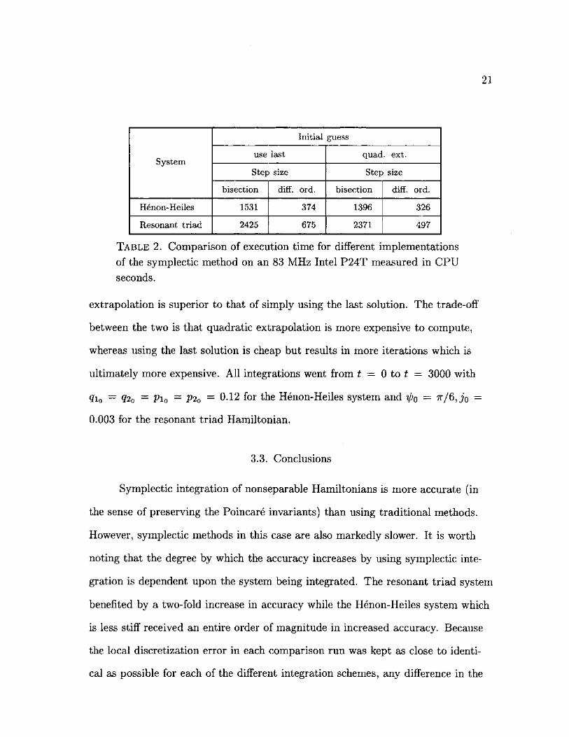
zero-crossing.f90

MODULE zero_crossing

USE f90_kind

IMPLICIT NONE

SAVE

PRIVATE

PUBLIC :: test_zero_crossing, zero_crossing_time

REAL(KIND=DOUBLE), DIMENSION(0:2) :: x_history, t.history

LOGICAL :: first.call-.TRUE.

CONTAINS

LOGICAL FUNCTION test_zero_crossing(x,t)

! Input: x at t, t

! Output: .TRUE, if crossed zero, .FALSE, otherwise

! x at t and t are recorded for future interpolations if t

! is different from the t given when last called.

IMPLICIT NONE

REAL(KIND=DQUBLE), INTENT(IN) :: x, t

IF (first.call) THEN

first.call « .FALSE.

xJiistory(O) = x

x_history(l) « x

x_history(2) = x

t.history(0) * t-10.0**EXP0NENT(t)

t.history(1) = t-0.5*10.0**EXP0NENT(t)

t_history(2) = t

ELSE

30 IF (ABS(t-tJiistory(2))>EPSIL0N(t)) THEN

x„history(0) = x_history(l)

x.history(l) = x_history(2)

x_history(2) = x

t.history(0) = t.history(l)

t.history(l) = t.history(2)

t.history(2) - t

END IF

END IF

IF ((ABS(xXEPSILON(x)).OR. (x*x.history(1)<0.0)) THEN

test.zero.crossing = .TRUE.

ELSE

test.zero.crossing = .FALSE.

END IF

END FUNCTION test.zero.crossing

49

50

60

REAL(KIND=D0UBLE) FUNCTION zero.crossing.timeQ

! Output: t at x=0.0, t(l) < t <= t(2)

! t is determined quadratically.

IMPLICIT NONE

REAL(KIND-DOUBLE), DIMENSION(0:2) :: alpha, beta, gamma

beta(O) = t.history(0)**2

beta(l) = t.history(l)-t.history(0)

gamma(l) = t.history(l)**2-beta(0)

gamma(2) = (t.history(2)-t.history(0))/beta(l)

beta(2) = t.history(2)**2-beta(0)-gamma(l)*gamma(2)

alpha(2) = (x_history(2)-x.history(0)-(x.history(l)-x.history(0))* ft

gamma(2))/beta(2)

alpha (1) = (x.history(l)-x„history(0)-alpha(2)*gamma(l))/beta(l)

alpha(0) = x.history(O) - alpha(l)*t.history(0) - alpha(2)#beta(0)

IF (ABS(alpha(2))>EPSILON(alpha(2))) THEN

gamma(O) » (alpha(l)**2-4.0*alpha(0)*alpha(2))**0.5

zero.crossing.time « 0.5*(-alpha(l)+gamma(0))/alpha(2)

IF (t.history(l)<t.history(2)) THEN

IF ((zero.cross ing.time<=t.history(1)).OR. ft

(zero_crossing.time>t.history(2))) ft

zero.crossing.time = 0.5#(-alpha(l)-gamma(0))/alpha(2)

ELSE

IF ((zero.crossing.time>=t .history (1)).OR. ft

(zero.crossing.time<t.history(2))) ft

zero.crossing.time = 0.5*(-alpha(l)-gamma(0))/alpha(2)

END IF

ELSE

zero.crossing.time * -alpha(0)/alpha(l)

80 END IF

END FUNCTION zero.crossing.time

END MODULE zero.crossing

70

REFERENCES

1. V.I. Arnold, Mathematical Methods of Classical Mechanics, Springer-Verlag,

New York, 1989, p. 163-168.

2. Herbert Goldstein, Classical Mechanics, 2nd Ed., Addison-Wesley, Reading,

Mass., 1980, p. 393.

3. J.M. Sanz-Serna and M.P. Calvo, Numerical Hamiltonian Problems, Chapman

& Hall, New York, 1994.

4. Channell, P.J. and Scovell, C., Symplectic integration of Hamiltonian systems,

Nonlinearity 3 (1990), 231-259.

5. Suris, Y.B., Preservation of symplectic structure in the numerical solution of

Hamiltonian systems Numerical Solution of Differential Equations (Filippov,

S.S., ed.), Akad. Nauk. SSSR, Inst. Prikl. Mat., 1988, pp. 148-160.

6. Sanz-Serna, J.M., Runge-Kutta schemes for Hamiltonian systems, BIT 28,

887-883.

7. David Kahaner, Cleve Moler, and Stephen Nash, Numerical Methods and

Software, Prentice Hall, New Jersey, 1989, pp. 141-145.

8. Shampine, L.F. and Gladwell, I., The next generation of Runge-Kutta codes

Computational Ordinary Differential Equations (Cash, J.R. and Gladwell, I.,

eds.), Clarendon Press, Oxford, 1992, pp. 145-164.

9. William H. Press, Brian P. Flannery, Saul A. Teukolsky, and William T. Vet-

terling, Numerical Recipes in C, Cambridge University Press, Cambridge,

51

1988, pp. 574-577.

10. Latka, M. and West, B.J., Structure of the stochastic layer of a perturbed res-

onant triad, Phys. Rev. E 52 (1995), no. 3, 3252-3255.

11. Latka, M. and West, B.J. (unpublished).

12. Trulsen, K. and Mei, C.C., J. Fluid Mech. 290 (1995), 345.

13. Craik, A.D.D., Wave Interactions and Fluid Flows, Cambridge University

Press, Cambridge, 1985.