On Symplectic Reduction in Classical Mechanics

J. Butterfield1

All Souls CollegeOxford OX1 4AL

Thursday 21 July 2005; a Chapter of The North Holland Handbook of Philosophy ofPhysics

Abstract

This Chapter expounds the modern theory of symplectic reduction in finite-dimensional Hamiltonian mechanics. This theory generalizes the well-known con-nection between continuous symmetries and conserved quantities, i.e. Noether’stheorem. It also illustrates one of mechanics’ grand themes: exploiting a sym-metry so as to reduce the number of variables needed to treat a problem. Theexposition emphasises how the theory provides insights about the rotation groupand the rigid body. The theory’s device of quotienting a state space also castslight on philosophical issues about whether two apparently distinct but utterlyindiscernible possibilities should be ruled to be one and the same. These issuesare illustrated using “relationist” mechanics.

Mottoes

The current vitality of mechanics, including the investigation of fundamental questions,is quite remarkable, given its long history and development. This vitality comes aboutthrough rich interactions with pure mathematics (from topology and geometry to grouprepresentation theory), and through new and exciting applications to areas like controltheory. It is perhaps even more remarkable that absolutely fundamental points, suchas a clear and unambiguous linking of Lie’s work on the Lie-Poisson bracket on thedual of a Lie algebra ... with the most basic of examples in mechanics, such as therigid body and the motion of ideal fluids, took nearly a century to complete.

Marsden and Ratiu (1999, pp. 431-432).

In the ordinary theory of the rigid body, six different three-dimensional spaces IR3, IR3∗, g,g∗, TGg, T

∗Gg are identified.Arnold (1989, p. 324).

1email: jb56@cus.cam.ac.uk; jeremy.butterfield@all-souls.oxford.ac.uk

Contents

1 Introduction 4

1.1 Why classical mechanics? . . . . . . . . . . . . . . . . . . . . . . . . . . 4

1.2 Prospectus . . . . . . . . . . . . . . . . . . . . . . . . . . . . . . . . . . 7

2 Symplectic reduction: an overview 10

2.1 Hamiltonian mechanics and Noether’s theorem: a review . . . . . . . . 10

2.1.1 Symplectic manifolds; the cotangent bundle as a symplectic man-ifold . . . . . . . . . . . . . . . . . . . . . . . . . . . . . . . . . 10

2.1.2 Geometric formulations of Hamilton’s equations . . . . . . . . . 13

2.1.3 Noether’s theorem . . . . . . . . . . . . . . . . . . . . . . . . . 13

2.2 The road ahead . . . . . . . . . . . . . . . . . . . . . . . . . . . . . . . 16

2.3 Appetizer: Belot on relationist mechanics . . . . . . . . . . . . . . . . . 19

2.3.1 Comparing two quotienting procedures . . . . . . . . . . . . . . 19

2.3.2 The spaces and group actions introduced . . . . . . . . . . . . . 21

2.3.3 The Relationist procedure . . . . . . . . . . . . . . . . . . . . . 23

2.3.4 The Reductionist procedure . . . . . . . . . . . . . . . . . . . . 25

2.3.5 Comparing the Relationist and Reductionist procedures . . . . . 28

3 Some geometric tools 31

3.1 Vector fields on manifolds . . . . . . . . . . . . . . . . . . . . . . . . . 31

3.1.1 Manifolds, vectors, curves and derivatives . . . . . . . . . . . . . 31

3.1.2 Vector fields, integral curves and flows . . . . . . . . . . . . . . 32

3.1.3 The Lie derivative . . . . . . . . . . . . . . . . . . . . . . . . . 35

3.2 Lie algebras and brackets . . . . . . . . . . . . . . . . . . . . . . . . . . 37

3.2.1 Lie algebras . . . . . . . . . . . . . . . . . . . . . . . . . . . . . 37

3.2.2 The Lie bracket of two vector fields . . . . . . . . . . . . . . . . 39

3.3 Submanifolds and Frobenius’ theorem . . . . . . . . . . . . . . . . . . . 41

3.3.1 Submanifolds . . . . . . . . . . . . . . . . . . . . . . . . . . . . 41

3.3.2 The theorem . . . . . . . . . . . . . . . . . . . . . . . . . . . . . 43

3.4 Lie groups, and their Lie algebras . . . . . . . . . . . . . . . . . . . . . 45

3.4.1 Lie groups and matrix Lie groups . . . . . . . . . . . . . . . . . 45

3.4.2 The Lie algebra of a Lie group . . . . . . . . . . . . . . . . . . . 46

1

3.4.3 Examples, subgroups and subalgebras . . . . . . . . . . . . . . . 50

3.4.4 The Lie algebra of the rotation group . . . . . . . . . . . . . . . 53

4 Actions of Lie groups 56

4.1 Basic definitions and examples . . . . . . . . . . . . . . . . . . . . . . . 57

4.2 Quotient structures from group actions . . . . . . . . . . . . . . . . . . 63

4.3 Proper actions . . . . . . . . . . . . . . . . . . . . . . . . . . . . . . . . 64

4.4 Infinitesimal generators of actions . . . . . . . . . . . . . . . . . . . . . 66

4.5 The adjoint and co-adjoint representations . . . . . . . . . . . . . . . . 68

4.5.1 The adjoint representation . . . . . . . . . . . . . . . . . . . . . 69

4.5.2 The co-adjoint representation . . . . . . . . . . . . . . . . . . . 72

4.6 Kinematics on Lie groups . . . . . . . . . . . . . . . . . . . . . . . . . 75

4.6.1 Space and body coordinates generalized to G . . . . . . . . . . . 75

4.6.2 Passage to the quotients . . . . . . . . . . . . . . . . . . . . . . 76

5 Poisson manifolds 79

5.1 Preamble: three reasons for Poisson manifolds . . . . . . . . . . . . . . 79

5.2 Basics . . . . . . . . . . . . . . . . . . . . . . . . . . . . . . . . . . . . 83

5.2.1 Poisson brackets . . . . . . . . . . . . . . . . . . . . . . . . . . 84

5.2.2 Hamiltonian vector fields . . . . . . . . . . . . . . . . . . . . . . 85

5.2.3 Structure functions . . . . . . . . . . . . . . . . . . . . . . . . . 86

5.2.4 The Poisson structure on g∗ . . . . . . . . . . . . . . . . . . . . 88

5.3 The symplectic foliation of Poisson manifolds . . . . . . . . . . . . . . . 91

5.3.1 The Poisson structure and its rank . . . . . . . . . . . . . . . . 91

5.3.2 Poisson maps . . . . . . . . . . . . . . . . . . . . . . . . . . . . 93

5.3.3 Poisson submanifolds: the foliation theorem . . . . . . . . . . . 94

5.3.4 Darboux’s theorem . . . . . . . . . . . . . . . . . . . . . . . . . 97

5.4 The symplectic structure of the co-adjoint representation . . . . . . . . 98

5.5 Quotients of Poisson manifolds . . . . . . . . . . . . . . . . . . . . . . . 100

6 Symmetry and conservation revisited: momentum maps 102

6.1 Canonical actions and momentum maps . . . . . . . . . . . . . . . . . 102

6.1.1 Canonical actions and infinitesimal generators . . . . . . . . . . 103

6.1.2 Momentum maps introduced . . . . . . . . . . . . . . . . . . . . 105

2

6.2 Conservation of momentum maps: Noether’s theorem . . . . . . . . . 107

6.3 Examples . . . . . . . . . . . . . . . . . . . . . . . . . . . . . . . . . . 108

6.4 Equivariance of momentum maps . . . . . . . . . . . . . . . . . . . . . 110

6.4.1 Equivariance and infinitesimal equivariance . . . . . . . . . . . . 111

6.4.2 Equivariant momentum maps are Poisson . . . . . . . . . . . . 112

6.5 Momentum maps on cotangent bundles . . . . . . . . . . . . . . . . . . 113

6.5.1 Momentum functions . . . . . . . . . . . . . . . . . . . . . . . . 113

6.5.2 Momentum maps for cotangent lifted actions . . . . . . . . . . . 114

6.5.3 Examples . . . . . . . . . . . . . . . . . . . . . . . . . . . . . . 116

7 Reduction 118

7.1 Preamble . . . . . . . . . . . . . . . . . . . . . . . . . . . . . . . . . . 118

7.2 The Lie-Poisson Reduction Theorem . . . . . . . . . . . . . . . . . . . 119

7.3 Meshing with the symplectic structure on T ∗G: invariant functions . . 120

7.3.1 Left-invariant and right-invariant functions on T ∗G . . . . . . . 121

7.3.2 Recovering the Lie-Poisson bracket . . . . . . . . . . . . . . . . 122

7.3.3 Deriving the Lie-Poisson bracket . . . . . . . . . . . . . . . . . . 123

7.4 Reduction of dynamics . . . . . . . . . . . . . . . . . . . . . . . . . . . 124

7.5 Envoi: the Marsden-Weinstein-Meyer theorem . . . . . . . . . . . . . . 126

8 References 128

3

1 Introduction

1.1 Why classical mechanics?

All hail the rise of modern physics! Between 1890 and 1930, the quantum and rela-tivity revolutions and the consolidation of statistical physics through the discovery ofatoms, utterly transformed our understanding of nature; and had an enormous influ-ence on philosophy; (e.g. Kragh 1999; Ryckman 2005). Accordingly, this Handbookconcentrates on those three pillars of modern physics—quantum theories, spacetimetheories and thermal physics. So some initial explanation of the inclusion of a Chapteron classical mechanics, indeed the classical mechanics of finite-dimensional systems, isin order.

The first point to make is that the various fields of classical physics, such as mechan-ics and optics, are wonderfully rich and deep, not only in their technicalities, but alsoin their implications for the philosophy and foundations of physics. From Newton’stime onwards, classical mechanics and optics have engendered an enormous amountof philosophical reflection. As regards mechanics, the central philosophical topics areusually taken (and have traditionally been taken) to be space, time, determinism andthe action-at-a-distance nature of Newtonian gravity. Despite their importance, I willnot discuss these topics; but some other Chapters will do so (at least in part, andsometimes in connection with theories other than classical mechanics). I will insteadfocus on the theory of symplectic reduction, which develops the well-known connectionbetween continuous symmetries and conserved quantities, summed up in Noether’s“first theorem”. I choose this focus partly by way of preparation for parts of someother Chapters; and partly because, as we will see in a moment, symplectic reductionplays a central role in the current renaissance of classical mechanics, and in its relationto quantum physics.

I said that classical physics engendered a lot of philosophical reflection. It is worthstressing two, mutually related, reasons for this: reasons which today’s philosophicalemphasis on the quantum and relativity revolutions tends to make us forget.

First: in the two centuries following Newton, these fields of classical physics weretransformed out of all recognition, so that the framework for philosophical reflectionabout them also changed. Think of how in the nineteenth century, classical mechanicsand optics gave rise to classical field theories, especially electromagnetism. And withinthis Chapter’s specific field, the classical mechanics of finite-dimensional systems, thinkof how even its central theoretical principles were successively recast, in fundamentalways, by figures such Euler, Lagrange, Hamilton and Jacobi.

Second, various difficult problems beset the attempt to rigorously formulate classi-cal mechanics and optics; some of which have considerable philosophical aspects. It isnot true that once we set aside the familiar war-horse topics—space, time, determinismand action-at-a-distance—the world-picture of classical mechanics is straightforward:just “matter in motion”. On the contrary. Even if we consider only finite-dimensional

4

systems, we can ask, for example:(i) For point-particles (material points): can they have different masses, and if

so how? What happens when they collide? Indeed, for point-particles interacting onlyby Newtonian gravity, a collision involves infinite kinetic energy.

(ii) For extended bodies treated as finite-dimensional because rigid: what hap-pens when they collide? Rigidity implies that forces, and displacements, are transmit-ted “infinitely fast” through the body. Surely that should not be taken literally? Butif so, what justifies this idealization; and what are its scope and limits?

As to infinite-dimensional systems (elastic solids, fluids and fields), many parts oftheir theories remain active research areas, especially as regards rigorous formulationsand results. For contemporary work on elastic solids, for example, cf. Marsden andHughes (1982). As to fluids, the existence and uniqueness of rigorous solutions of themain governing equations, the Navier-Stokes equations, is still an open problem. Thisproblem not only has an obvious bearing on determinism; it is regarded as scientifi-cally significant enough that its solution would secure a million-dollar Clay Millenniumprize.

These two reasons—the successive reformulations of classical mechanics, and itsphilosophical problems—are of course related. The monumental figures of classicalmechanics recognized and debated the problems, and much of their technical workwas aimed at solving them. As a result, there was a rich debate about the founda-tions of classical physics, in particular mechanics, for the two centuries after Newton’sPrincipia (1687). A well-known example is Duhem’s instrumentalist philosophy ofscience, which arose in large measure from his realization how hard it was to securerigorous foundations at the microscopic level for classical mechanics. A similar exam-ple is Hilbert’s being prompted by his contemporaries’ continuing controversies aboutthe foundations of mechanics, to choose as the sixth of his famous list of outstand-ing mathematical problems, the axiomatization of mechanics and probability; (but forsome history of this list, cf. Grattan-Guinness (2000)). A third example, spanningboth centuries, concerns variational principles: the various principles of least actionformulated first by Maupertuis, then by Euler and later figures—first for finite classi-cal mechanical systems, then for infinite ones—prompted much discussion of teleology.Indeed, this discussion ensnared the logical empiricists (Stoltzner 2003); it also bearson contemporary philosophy of modality (Butterfield 2004).

In the first half of the twentieth century, the quantum and relativity revolutionstended to distract physicists, and thereby philosophers, from these and similar prob-lems. The excitement of developing the new theories, and of debating their implicationsfor natural philosophy, made it understandable, even inevitable, that the foundationalproblems of classical mechanics were ignored.

Besides, this tendency was strengthened by the demands of pedagogy: the neces-sity of including the new theories in physics undergraduate degrees. By mid-century,the constraints of time on the physics curriculum had led many physics undergradu-ates’ education in classical mechanics to finish with the elementary parts of analytical

5

mechanics, especially of finite-dimensional systems: for example, with the materialin Goldstein’s well-known textbook (1950). Such a restriction is understandable, notleast because: (i) the elementary theory of Lagrange’s and Hamilton’s equations re-quires knowledge of ordinary differential equations, and (ii) elementary Hamiltonianmechanics forms a springboard to learning elementary canonical quantization (as doesHamilton-Jacobi theory, from another perspective). Besides, as I mentioned: even thisrestricted body of theory provides plenty of material for philosophical analysis—witnessmy examples above, and the discussions of the great figures such Euler, Lagrange,Hamilton and Jacobi.

However, the second half of the twentieth century saw a renaissance in research inclassical mechanics: hence my first motto. There are four obvious reasons for this: thefirst two “academic”, and the second two “practical”.

(i): Thanks partly to developments in mathematics in the decades after Hilbert’slist of problems, the foundational questions were addressed afresh, as much by math-ematicians and mathematically-minded engineers as by physicists. The most relevantdevelopments lay in such fields as topology, differential geometry, measure theory andfunctional analysis. In this revival, the contributions of the Soviet school, always strongin mechanics and probability, were second to none. And relatedly:—

(ii): The quest to deepen the formulation of quantum theory, especially quantumfield theory, prompted investigation of (a) the structure of classical mechanics and (b)quantization. For both (a) and (b), special interest attaches to the generally muchharder case of infinite systems.

(iii): The coming of spaceflight, which spurred the development of celestial mechan-ics. And relatedly:—

(iv): The study of non-linear dynamics (“chaos theory”), which was spurred by theinvention of computers.

With these diverse causes and aspects, this renaissance continues to flourish—andaccordingly, I shall duck out of trying to further adumbrate it! I shall even duck outof trying to survey the philosophical questions that arise from the various formulationsof mechanics from Newton to Jacobi and Poincare. Suffice it to say here that to thevarious topics mentioned above, one could add, for example, the following two: thefirst broadly ontological, the second broadly epistemological.

(a): The analysis of notions such as mass and force (including how they changeover time). For this topic, older books include Jammer (1957, 1961) and McMullin(1978); recent books include Boudri (2002), Jammer (2000), Lutzen (2005) and Slovik(2002); and Grattan-Guinness (2006) is a fine recent synopsis of the history, with manyreferences.

(b): The analysis of what it is to have an explicit solution of a mechanical problem(including how the notion of explicit solution was gradually generalized). This topic ismulti-faceted. It not only relates to the gradual generalization of the notion of function(a grand theme in the history of mathematics—well surveyed by Lutzen 2003), andto modern non-linear dynamics (cf. (iv) above). It also relates to the simplificationof problems by exploiting a symmetry so as to reduce the number of variables one

6

needs—and this is the core idea of symplectic reduction. I turn to introducing it.

1.2 Prospectus

The strategy of simplifying a mechanical problem by exploiting a symmetry so asto reduce the number of variables is one of classical mechanics’ grand themes. It istheoretically deep, practically important, and recurrent in the history of the subject.The best-known general theorem about the strategy is undoubtedly Noether’s theo-rem, which describes a correspondence between continuous symmetries and conservedquantities. There is both a Lagrangian and a Hamiltonian version of this theorem,though for historical reasons the name ‘Noether’s theorem’ is more strongly attachedto the Lagrangian version. However, we shall only need the Hamiltonian version of thetheorem: it will be the “springboard” for our exposition of symplectic reduction.2

So I shall begin by briefly reviewing the Hamiltonian version in Section 2.1. Forthe moment, suffice it to make four comments (in ascending order of importance forwhat follows):

(i): Both versions are underpinned by the theorems in elementary Lagrangian andHamiltonian mechanics about cyclic (ignorable) coordinates and their correspondingconserved momenta.3

(ii): In fact, the Hamiltonian version of the theorem is stronger. This reflects thefact that the canonical transformations form a “larger” group than the point trans-formations. A bit more precisely: though the point transformations q → q′ on theconfiguration space Q induce canonical transformations on the phase space Γ of the qsand ps, q → q′, p→ p′ , there are yet other canonical transformations which “mix” theqs and ps in ways that transformations induced by point transformations do not.

(iii): I shall limit our discussion to (a) time-independent Hamiltonians and (b)time-independent transformations. Agreed, analytical mechanics can be developed, inboth Lagrangian and Hamiltonian frameworks, while allowing time-dependent dynam-ics and transformations. For example, in the Lagrangian framework, allowing velocity-

2For discussion of the Lagrangian version, cf. e.g. Brading and Castellani (this vol., ch. 13)or (restricted to finite-dimensional systems) Butterfield (2004a: Section 4.7). For an exposition ofboth versions that is complementary to this paper (and restricted to finite-dimensional systems), cf.Butterfield (2006). Brading and Castellani also bring out that, even apart from Noether’s theoremsin other branches of mathematics, there are other ‘Noether’s theorems’ about symmetries in classicaldynamics; so the present theorem is sometimes called Noether’s “first theorem”. Note also (though Ishall not develop this point) that symplectic structure can be seen in the classical solution space ofLagrange’s equations, so that symplectic reduction can be developed in the Lagrangian framework;cf. e.g. Marsden and Ratiu (1999: p. 10, Sections 7.2-7.5, and 13.5).

3Here we glimpse the long history of our subject: these theorems were of course clear to thesesubjects’ founders. Indeed the strategy of exploiting a symmetry to reduce the number of variablesoccurs already in 1687, in Newton’s solution of the Kepler problem; (or more generally, the problemof two bodies exerting equal and opposite forces along the line between them). The symmetries aretranslations and rotations, and the corresponding conserved quantities are the linear and angularmomenta. In what follows, these symmetries and quantities will provide us with several examples.

7

dependent potentials and-or time-dependent constraints would prompt one to use whatis often called the ‘extended configuration space’ Q×IR. And in the Hamiltonian frame-work, time-dependence prompts one to use an ‘extended phase space’ Γ× IR. Besides,from a philosophical viewpoint, it is important to consider time-dependent transfor-mations: for they include boosts, which are central to the philosophical discussion ofspacetime symmetry groups, and especially of relativity principles. But beware: rough-and-ready statements about symmetry, e.g. that the Hamiltonian must be invariantunder a symmetry transformation, are liable to stumble on these transformations. Togive the simplest example: the Hamiltonian of a free particle is just its kinetic energy,which can be made zero by transforming to the particle’s rest frame; i.e. it is notinvariant under boosts.

So a full treatment of symmetry in Hamiltonian mechanics, and thereby of sym-plectic reduction, needs to treat time-dependent transformations—and to beware! ButI will set aside all these complications. Here it must suffice to assert, without anydetails, that the modern theory of symplectic reduction does cope with boosts; andmore generally, with time-dependent dynamics and transformations.

(iv): As we shall see in detail, there are three main ways in which the theory ofsymplectic reduction generalizes Noether’s theorem. As one might expect, these threeways are intimately related to one another.

(a): Noether’s theorem is “one-dimensional” in the sense that for each sym-metry (a vector field of a special kind on the phase space), it provides a conservedquantity, i.e. a real-valued function on the phase space, whose value stays constantover time. So in particular, different components of a conserved vector quantity, suchas total linear momentum, are treated separately; (in this example, the correspondingvector fields generate translations in three different spatial directions). But in sym-plectic reduction, the notion of a momentum map provides a “unified” description ofthese different components.

(b): Given a symmetry, Noether’s theorem enables us to confine our attentionto the level surface of the conserved quantity, i.e. the sub-manifold of phase space onwhich the quantity takes its initial value: for the system’s time-evolution is confinedto that surface. In that sense, the number of variables we need to consider is reduced.But in symplectic reduction, we go further and form a quotient space from the phasespace. That is, in the jargon of logic: we define on phase space an equivalence relation(not in general so simple as having a common value for a conserved quantity) and formthe set of equivalence classes. In the jargon of group actions: we form the set of orbits.Passage to this quotient space can have various good technical, and even philosophi-cal, motivations. And under good conditions, this set is itself a manifold with lowerdimension.

(c): Hamiltonian mechanics, and so Noether’s theorem, is usually formulatedin terms of symplectic manifolds, in particular the cotangent bundle T ∗Q of the con-figuration space Q. (Section 2.1 will give details.) But in symplectic reduction, weoften need a (mild) generalization of the idea of a symplectic manifold, called a Pois-son manifold, in which a bracket, with some of the properties of the Poisson bracket,

8

is taken as the primitive notion. Besides, this is related to (b) in that we are oftenled to a Poisson manifold, and dynamics on it, by taking the quotient of a symplecticmanifold (i.e. a phase space of the usual kind) by the action of a symmetry group.

As comment (iv) hints, symplectic reduction is a large subject. So there are severalmotivations for expounding it. As regards physics, many of the ideas and results canbe developed for finite-dimensional classical systems (to which I will confine myself),but then generalized to infinite-dimensional systems. And in either the original or thegeneralized form, they underpin developments in quantum theories. So these ideas andresults have formed part of the contemporary renaissance in classical mechanics; cf. (i)and (ii) at the end of Section 1.1.

As regards philosophy, symmetry is both a long-established focus for philosophi-cal discussion, and a currently active one: cf. Brading and Castellani (2003). Butphilosophical discussion of symplectic reduction seems to have begun only recently,especially in some papers of Belot and Earman. This delay is presumably because thetechnical material is more sophisticated: indeed, the theory of symplectic reductionwas cast in its current general form only in the 1970s. But as Belot and Earman em-phasise, the philosophical benefits are worth the price of learning the technicalities.The most obvious issue is that symplectic reduction’s device of quotienting a statespace casts light on philosophical issues about whether two apparently distinct bututterly indiscernible possibilities should be ruled to be one and the same. In Section2, I will follow Belot in illustrating this issue with “relationist” mechanics. Indeed, Ihave selected the topics for my exposition with an eye to giving philosophical readersthe background needed for some of Belot’s discussions. His papers (which I will citein Section 2) make many judicious philosophical points, without burdening the readerwith an exposition of technicalities: excellent stuff—but to fully appreciate the issues,one of course has to slog through the details.

Finally, in the context of this volume, symplectic reduction provides some back-ground for the Chapters on the representation of time in mechanics (Belot, this vol.,ch. 2), and on the relations between classical and quantum physics (Landsman, thisvol., ch. 5, especially Sections 4.3-4.5 and 6.5; Dickson, this vol., ch. 4).

The plan of the Chapter is as follows. I first review Noether’s theorem in Hamil-tonian mechanics as usually formulated, in Section 2.1. Then I introduce the themesmentioned in (b) and (c) above, of quotienting a phase space, and Poisson manifolds(Section 2.2); and illustrate these themes with “relationist” mechanics (Section 2.3).

Thereafter, I expound the basics of symplectic reduction: (confining myself to finite-dimensional Hamiltonian mechanics). Section by Section, the plan will be as follows.Sections 3 and 4 review the modern geometry that will be needed. Section 3 is mostlyabout Frobenius’ theorem, Lie algebras and Lie groups.4 Section 4 expounds Lie groupactions. It ends with the central idea of the co-adjoint representation of a Lie groupG on the dual g∗ of its Lie algebra. This review enables us to better understand the

4Its first two Subsections also provide some pre-requisites for Malament (this vol.).

9

motivations for Poisson manifolds (5.1); and then to exhibit examples, and prove somemain properties (Section 5.2 onwards). Section 6 applies this material to symmetry andconservation in mechanical systems. In particular, it expresses conserved quantities asmomentum maps, and proves Noether’s theorem for Hamiltonian mechanics on Poissonmanifolds. Finally, in Section 7, we prove one of the several main theorems aboutsymplectic reduction. It concerns the case where the natural configuration space fora system is itself a Lie group G: this occurs both for the rigid body and ideal fluids.In this case, quotienting the natural phase space (the cotangent bundle on G) gives aPoisson manifold that “is” the dual g∗ of G’s Lie algebra.5

To sum up:— The overall effect of this exposition is, I hope, to illustrate thisChapter’s mottoes: that classical mechanics is alive and kicking, not least throughdeepening our understanding of time-honoured systems such as the rigid body—whoseanalysis in traditional textbooks can be all too confusing!

2 Symplectic reduction: an overview

We begin by briefly reviewing Hamiltonian mechanics and Noether’s theorem, in Sec-tion 2.1.6 This prepares us for the idea of symplectic reduction, Section 2.2: which wethen illustrate using “relationist” mechanics, Section 2.3.

2.1 Hamiltonian mechanics and Noether’s theorem: a review

2.1.1 Symplectic manifolds; the cotangent bundle as a symplectic manifold

A symplectic structure or symplectic form on a manifoldM is defined to be a differential2-form ω on M that is closed (i.e. its exterior derivative dω vanishes) and is non-degenerate. That is: for any x ∈M , and any two tangent vectors at x, σ, τ ∈ Tx:

dω = 0 and ∀ τ �= 0, ∃σ : ω(τ, σ) �= 0 . (2.1)

Such a pair (M,ω) is called a symplectic manifold. There is a rich theory of symplecticmanifolds; but we shall only need a small fragment of it. (In particular, the fact thatwe mostly avoid the theory of canonical transformations means we will not need thetheory of Lagrangian sub-manifolds.)

5In this endeavour, my sources are four books by masters of the subject: Abraham and Marsden(1978), Arnold (1989), Marsden and Ratiu (1999) and Olver (2000). But again, be warned: myselection is severe, as anyone acquainted with these or similar books will recognize.

6For more details about differential geometry, cf. Sections 3.1 and 3.2. For more details aboutthe geometric formulation of mechanics, cf. Arnold (1989) or Marsden and Ratiu (1999); or Singer(2001) (more elementary than this exposition) or Abraham and Marsden (1978) (more advanced); orButterfield (2006) (at the same level). Of many good textbooks of mechanics, I admire especiallyDesloge (1982) and Johns (2005).

10

First, it follows from the non-degeneracy of ω that M is even-dimensional. Thereason lies in a theorem of linear algebra, which one then applies to the tangent spaceat each point of M . Namely, for any bilinear form ω : V ×V → IR: if ω is antisymmetricof rank r ≤ m ≡ dim(V ), then r is even. That is: r = 2n for some integer n, and thereis a basis e1, ..., ei, ..., em of V for which ω has a simple expansion as wedge-products

ω = Σni=1 e

i ∧ ei+n ; (2.2)

equivalently, ω has the m×m matrix

ω =

⎛⎝ 0 1 0

−1 0 00 0 0

⎞⎠ . (2.3)

where 1 is the n×n identity matrix, and similarly for the zero matrices of various sizes.This normal form of antisymmetric bilinear forms is an analogue of the Gram-Schmidttheorem that an inner product space has an orthonormal basis, and is proved by ananalogous argument.

So if an antisymmetric bilinear form is non-degenerate, then r ≡ 2n = m. That is:eq. 2.3 loses its bottom row and right column consisting of zero matrices, and reducesto the 2n× 2n symplectic matrix ω given by

ω :=

(0 1−1 0

). (2.4)

Second, the non-degeneracy of ω implies that at any x ∈ M , there is a basis-independent isomorphism ω� from the tangent space Tx to its dual T ∗

x . Namely: forany x ∈M and τ ∈ Tx, the value of the 1-form ω�(τ) ∈ T ∗

x is defined by

ω�(τ)(σ) := ω(σ, τ) ∀σ ∈ Tx . (2.5)

This also means that a symplectic structure enables a covector field, i.e. a differentialone-form, to determine a vector field. Thus for any function H : M → IR, so that dHis a differential 1-form on M , the inverse of ω� (which we might write as ω�), carriesdH to a vector field on M , written XH . This is the key idea whereby in Hamiltonianmechanics, a scalar function H determines a dynamics; cf. Section 2.1.2.

So far, we have noted some implications of ω being non-degenerate. The other partof the definition of a symplectic form (for a manifold), viz. ω being closed, dω = 0, isalso important. We shall see in Section 2.1.3 that it implies that a vector field X on asymplectic manifold M preserves the symplectic form ω (i.e. in more physical jargon:generates (a one-parameter family of) canonical transformations) iff X is Hamiltonianin the sense that there is a scalar function f such that X = Xf ≡ ω�(df). Or in termsof the Poisson bracket, with · representing the argument place for a scalar function:X(·) = Xf(·) ≡ {·, f}.

11

So much by way of introducing symplectic manifolds. I turn to showing that anycotangent bundle T ∗Q is such a manifold. That is: it has, independently of a choice ofcoordinates or bases, a symplectic structure.

Given a manifold Q (dim(Q)=n) which we think of as the system’s configurationspace, choose any local coordinate system q on Q , and the natural local coordinatesq, p thereby induced on T ∗Q. We define the 2-form

dp ∧ dq := dpi ∧ dqi := Σni=1dpi ∧ dqi . (2.6)

In fact, eq. 2.6 defines the same 2-form, whatever choice we make of the chart q on Q.For dp∧dq is the exterior derivative of a 1-form on T ∗Q which is defined naturally (i.e.independently of coordinates or bases) from the derivative (also known as: tangent)map of the projection

π : (q, p) ∈ T ∗Q → q ∈ Q. (2.7)

Thus consider a tangent vector τ (not to Q, but) to the cotangent bundle T ∗Q at apoint η = (q, p) ∈ T ∗Q, i.e. q ∈ Q and p ∈ T ∗

q . Let us write this as: τ ∈ Tη(T∗Q) ≡

T(q,p)(T∗Q). The derivative map, Dπ say, of the natural projection π applies to τ :

Dπ : τ ∈ T(q,p)(T∗Q) → (Dπ(τ)) ∈ Tq . (2.8)

Now define a 1-form θH on T ∗Q by

θH : τ ∈ T(q,p)(T∗Q) → p(Dπ(τ)) ∈ IR ; (2.9)

where in this definition of θH , p is defined to be the second component of τ ’s base-point(q, p) ∈ T ∗Q; i.e. τ ∈ T(q,p)(T

∗Q) and p ∈ T ∗q .

This 1-form is called the canonical 1-form on T ∗Q. One now checks that in anynatural local coordinates q, p, θH is given by

θH = pidqi. (2.10)

Finally, we define a 2-form by taking the exterior derivative of θH :

d(θH) := d(pidqi) ≡ dpi ∧ dqi . (2.11)

One checks that this 2-form is closed (since d2 = 0) and non-degenerate. So (T ∗Q,d(θH))is a symplectic manifold. Accordingly, d(θH), or its negative −d(θH), is called thecanonical symplectic form, or canonical 2-form.

There is a theorem (Darboux’s theorem) to the effect that locally, any symplecticmanifold “looks like” a cotangent bundle: or in other words, a cotangent bundle islocally a “universal” example of symplectic structure. We will not go into details; butin Section 5.3.4, we will discuss the generalization of this theorem for Poisson manifolds.But first we review, in the next two Subsections, Hamilton’s equations, and Noether’stheorem.

12

2.1.2 Geometric formulations of Hamilton’s equations

As we already emphasised, the main geometric idea behind Hamilton’s equations is thata gradient, i.e. covector, field dH determines a vector field XH . So to give a geometricformulation of Hamilton’s equations at a point x = (q, p) in a cotangent bundle T ∗Q,let us write ω� for the (basis-independent) isomorphism from the cotangent space tothe tangent space, T ∗

x → Tx, induced by ω := −d(θH) = dqi ∧ dpi (cf. eq. 2.5). ThenHamilton’s equations may be written as:

x = XH(x) = ω�(dH(x)) = ω�(dH(x)) . (2.12)

There are various other formulations. Applying ω�, the inverse isomorphism Tx → T ∗x ,

to both sides, we getω�XH(x) = dH(x) . (2.13)

In terms of the symplectic form ω at x, this is: for all vectors τ ∈ Tx

ω(XH(x), τ) = dH(x) · τ ; (2.14)

or in terms of the contraction (also known as: interior product) iXα of a differentialform α with a vector field X, with · marking the argument place of τ ∈ Tx:

iXHω := ω(XH(x), ·) = dH(x)(·) . (2.15)

More briefly, and now written for any function f , it is:

iXfω = df . (2.16)

Finally, recall the relation between the Poisson bracket and the directional derivative(or the Lie derivative L) of a function: viz.

LXfg = dg(Xf) = Xf(g) = {g, f} . (2.17)

Combining this with eq. 2.16, we can state the relation between the symplectic formand Poisson bracket in the form:

{g, f} = dg(Xf) = iXfdg = iXf

(iXgω) = ω(Xg, Xf) . (2.18)

2.1.3 Noether’s theorem

The core idea of Noether’s theorem, in both the Lagrangian and Hamiltonian frame-works, is that to every continuous symmetry of the system there corresponds a con-served quantity (a first integral, a constant of the motion). The idea of a continuoussymmetry is made precise along the following lines: a symmetry is a vector field onthe state-space that (i) preserves the Lagrangian (respectively, Hamiltonian) and (ii)“respects” the structure of the state-space.

13

In the Hamiltonian framework, the heart of the proof is a “one-liner” based on thefact that the Poisson bracket is antisymmetric. Thus for any scalar functions f and Hon a symplectic manifold (M,ω) (and so with a Poisson bracket given by eq. 2.18), wehave that at any point x ∈M

Xf(H)(x) ≡ {H, f}(x) = 0 iff 0 = {f,H}(x) ≡ XH(f)(x) . (2.19)

In words: around x, H is constant under the flow of the vector field Xf (i.e. underwhat the evolution would be if f was the Hamiltonian) iff f is constant under the flowXH . Thinking of H as the physical Hamiltonian, so that XH represents the real time-evolution (sometimes called: the dynamical flow), this means: around x, Xf preservesthe Hamiltonian iff f is constant under time-evolution, i.e. f is a conserved quantity(a constant of the motion).

But we need to be careful about clause (ii) above: the idea that a vector field re-spects” the structure of the state-space. In the Hamiltonian framework, this is madeprecise as preserving the symplectic form. Thus we define a vector field X on a symplec-tic manifold (M,ω) to be symplectic (also known as: canonical) iff the Lie-derivativealong X of the symplectic form vanishes, i.e. LXω = 0. (This definition is equivalentto X’s generating (active) canonical transformations, and to its preserving the Poissonbracket. But I will not go into details about these equivalences: for they belong to thetheory of canonical transformations, which, as mentioned, I will not need to develop.)

We also define a Hamilton system to be a triple (M,ω,H) where (M,ω) is a sym-plectic manifold and H : M → IR, i.e. M ∈ F(M). And then we define a (continuous)symmetry of a Hamiltonian system to be a vector field X on M that:

(i) preserves the Hamiltonian function, LXH = 0; and(ii) preserves the symplectic form, LXω = 0.

These definitions mean that to prove Noether’s theorem from eq. 2.19, it will sufficeto prove that a vector field X is symplectic iff it is locally of the form Xf . Such a vectorfield is called locally Hamiltonian. (And a vector field is called Hamiltonian if there isa global scalar f : M → IR such that X = Xf .) In fact, two results from the theory ofdifferential forms, the Poincare Lemma and Cartan’s magic formula, make it easy toprove this; (for a vector field on any symplectic manifold (M,ω), i.e. (M,ω) does notneed to be a cotangent bundle).

Again writing d for the exterior derivative, we recall that a k-form α is called:(i): exact if there is a (k−1)-form β such that α = dβ; (cf. the elementary definition

of an exact differential);(ii): closed if dα = 0.

The Poincare Lemma states that every closed form is locally exact. To be precise: forany open set U of M , we define the vector space Ωk(U) of k-form fields on U . Thenthe Poincare Lemma states that if α ∈ Ωk(M) is closed, then at every x ∈ M there isa neighbourhood U such that α |U ∈ Ωk(U) is exact.

Cartan’s magic formula is a useful formula (proved by straightforward calculation)relating the Lie derivative, contraction and the exterior derivative. It says that if X

14

is a vector field and α a k-form on a manifold M , then the Lie derivative of α withrespect to X (i.e. along the flow of X) is

LXα = diXα + iXdα . (2.20)

We now argue as follows. Since ω is closed, i.e. dω = 0, Cartan’s magic formula,eq. 2.20, applied to ω becomes

LXω ≡ diXω + iXdω = diXω . (2.21)

So for X to be symplectic is for iXω to be closed. But by the Poincare Lemma, if iXωclosed, it is locally exact. That is: there locally exists a scalar function f : M → IRsuch that

iXω = df i.e. X = Xf . (2.22)

So for X to be symplectic is equivalent to X being locally Hamiltonian.

Thus we have

Noether’s theorem for a Hamilton system If X is a symmetry ofa Hamiltonian system (M,ω,H), then locally X = Xf ; so by the anti-symmetry of the Poisson bracket, eq. 2.19, f is a constant of the motion.And conversely: if f : M → IR is a constant of the motion, then Xf is asymmetry.

We will see in Section 6.2 that most of this approach to Noether’s theorem, inparticular the “one-liner” appeal to the anti-symmetry of the Poisson bracket, eq. 2.19,carries over to the more general framework of Poisson manifolds. For the moment, wemention an example (which we will also return to).

For most Hamiltonian systems in euclidean space IR3, spatial translations and ro-tations are (continuous) symmetries. Let us consider in particular a system we willdiscuss in more detail in Section 2.3: N point-particles interacting by Newtonian grav-ity. The Hamiltonian is a sum of two terms, which are each individually invariantunder translations and rotations:

(i) a kinetic energy term K; though I will not go into details, it is in fact definedby the euclidean metric of IR3, and is thereby invariant; and

(ii) a potential energy term V ; it depends only on the particles’ relative distances,and is thereby invariant.

The corresponding conserved quantities are the total linear and angular momen-tum.7

7By the way, this Hamiltonian is not invariant under boosts. But as I said in (iii) of Section 1.2, Irestrict myself to time-independent transformations; the treatment of symmetries that “represent therelativity of motion” needs separate discussion.

15

2.2 The road ahead

In this Subsection, four comments will expand on the introductory comment (iv) ofSection 1.2, and also give some information about the history of symplectic reductionand about some crucial examples.

(1): Generalizing from Noether’s theorem; Poisson manifolds:—Noether’s theorem tells us that a continuous symmetry, i.e. a one-parameter group ofsymmetries, determines a first integral (i.e. a constant of the motion). So a larger groupof symmetries, i.e. a group with several parameters, implies several first integrals. Thephase flow is therefore confined to the intersection of the level surfaces of these integrals:an intersection which is in general a manifold. In other words: the simultaneous levelmanifold of these integrals is an invariant manifold of the phase flow.

It turns out that, in many useful cases, this manifold is also invariant under anappropriately chosen subgroup of the group of symmetries; and that the quotient space,i.e. the set of orbits under the action of this subgroup, is a manifold with a naturalstructure induced by the original Hamiltonian system that is sufficient to do mechanicsin Hamiltonian style. The quotient space is therefore called the ‘reduced phase space’.

But in some cases, this natural structure is not a symplectic form, but a (mild)generalization in which the the form is allowed to be degenerate; i.e. like eq. 2.3rather than eq. 2.4. A manifold equipped with such a structure need not be a quotientmanifold. It can instead be defined in terms of a generalization of the usual Poissonbracket, as defined in terms of the symplectic form by eq. 2.18.

The key idea is to postulate a bracket, acting on the scalar functions F : M → IR onany manifold M , and possessing four properties enjoyed by the usual Poisson bracket.One of the properties is anti-symmetry, emphasised in Section 2.1.3’s proof of Noether’stheorem. The other three are that the postulated bracket, again written {, }, is: to bebilinear; to obey the Jacobi identity for any real functions F,G,H on M , i.e.

{{F,H}, G}+ {{G,F}, H}+ {{H,G}, F} = 0 ; (2.23)

and to obey Leibniz’ rule for products, i.e.

{F,H ·G} = {F,H} ·G+H · {F,G} . (2.24)

We will see in Section 5 that such a bracket, again called ‘Poisson bracket’, providesa sufficient framework for mechanics in Hamiltonian style. In particular, it induces ananti-symmetric bilinear form that may be degenerate, as in eq. 2.3. A manifold Mequipped with such a bracket is called a Poisson manifold.

The allowance of degeneracy means that a Poisson manifold can have odd dimension;while we saw in Section 2.1.1 that any symplectic manifold is even-dimensional. On theother hand, this generalized Hamiltonian mechanics will have clear connections withthe usual formulation of Section 2.1. The main connection will be the result that anyPoisson manifold M is a disjoint union of even-dimensional manifolds, on which M ’s

16

degenerate antisymmetric bilinear form restricts to be non-degenerate.8

(2): Historical roots:—The theory of symplectic reduction has deep historical roots in the work of classical me-chanics’ monumental figures. In part, this is no surprise. As mentioned in (i) of Section1.2, cyclic coordinates underpin the role of symmetry in mechanics, and in particularNoether’s theorem. And Newton’s solution of the Kepler problem provides an exam-ple: witness textbooks’ expositions of the transition to centre-of-mass coordinates, andof polar coordinates with the angle being cyclic (yielding angular momentum as theconserved quantity). So it is unsurprising that various results and ideas of symplecticreduction can be seen in the work of such masters as Euler, Lagrange, Hamilton, Ja-cobi, Lie and Poincare; for example (as we will see), in Euler’s theory of the rigid body.

But the history also holds a surprise. It turns out that Lie’s epoch-making work onLie groups already contained a detailed development of much of the general, moderntheory.9 The sad irony is that most of Lie’s insights were not taken up—and werethen repeatedly re-discovered. So this is yet another example (of which the history ofmathematics has so many!) of the saying that he who does not learn from history isdoomed to repeat it. The consolation is of course that it is often easier, and more fun,to re-discover something than to learn it from another...

Thus it was only from the mid-1960s that the theory, in essentially the form Liehad, was recovered and cast in the geometric language adopted by modern mechanics;namely, by contemporary masters such as Arnold, Kostant, Marsden, Meyer, Smale,Souriau and Weinstein; (cf. this Chapter’s first motto). Happily, several of these mod-ern authors are scholars of the history, and even their textbooks give some historicaldetails: cf. Marsden and Ratiu (1999, pp. 336-8, 369-370, 430-432), and the notes toeach Chapter of Olver (2000: especially p.427-428). (Hawkins (2000) is a full historyof Lie groups from 1869 to 1926; for Lie, cf. especially its Sections 1.3, 2.5 and Chapter3, especially 3.2.)

In any case, setting history aside: symplectic reduction has continued since the1970s to be an active research area in contemporary mechanics, and allied fields suchas symplectic geometry. So it has now taken its rightful place as a major part of thecontemporary renaissance of classical mechanics: as shown by ...

(3): Two examples: the rigid body and the ideal fluid:—Two examples illustrate vividly how symplectic reduction can give new physical un-derstanding, even of time-honoured examples: the rigid body and the ideal fluid—asattested by this Chapter’s mottoes. (Section 2.3 will develop a third example, moreclosely related to philosophy.)

As to the rigid body: we will see (especially in Section 5) that symplectic reductionconsiderably clarifies the elementary theory of the rigid body (Euler’s equations, Euler

8Because of these clear connections, it is natural to still call the more general framework ‘Hamil-tonian’; as is usually done. But of course this is just a verbal matter.

9The main source is his (1890). Besides, Arnold (1989: 456) reports that the prototype exampleof a Poisson manifold, viz. the dual of a finite-dimensional Lie algebra, was already understood byJacobi.

17

angles etc.): which, notoriously, can be all too confusing! For simplicity, I shall takethe rigid body to be pivoted, so as to set aside translational motion. This will meanthat the group of symmetries defining the quotienting procedure will be the rotationgroup. It will also mean that the rigid body’s configuration space is given by therotation group, since any configuration can be labelled by the rotation that obtains itfrom some reference-configuration. So in this application of symplectic reduction, thesymmetry group (viz. the rotation group) will act on itself as the configuration space.This example will also give us our prototype example of a Poisson manifold.

As to the ideal fluid, i.e. a fluid that is incompressible and inviscid (with zeroviscosity): this is of course an infinite-dimensional system, and so (as I announced inSection 1.2) outside the scope of this Chapter. So I will not go into any details, butjust report the main idea.

The equations of motion of an ideal fluid, Euler’s equations, are usually derivedeither by applying Newton’s second law F = ma to a small fluid element; or by aheuristic use of the Lagrangian or Hamiltonian approach (as in heuristic classical fieldtheories). But in the mid-1960s, Arnold showed how the latter derivations could beunderstood in terms of a striking, even beautiful, analogy with the above treatmentof the rigid body. Namely, the analogy shows that the configuration space of thefluid is an infinite-dimensional group; as follows. The configuration of an ideal fluidconfined to some container occupying a volume V ⊂ IR3 is an assignment to eachspatial position x ∈ V of an infinitesimal fluid element. Given such an assignmentas a reference-configuration, any other configuration can be labelled by the volume-preserving diffeomorphism d from V to V that carries the reference-configuration tothe given one, by dragging each fluid element along by d. So given a choice of reference-configuration, the fluid’s configuration space is given by the infinite-dimensional groupD of diffeomorphisms d : V → V : just as the rotation group is the configurationspace of a (pivoted) rigid body. D then forms the basis for rigorous Lagrangian andHamiltonian theories of an ideal fluid.

These theories turn out to have considerable analogies with the Lagrangian andHamiltonian theories of the rigid body, thanks to the fact that in both cases the sym-metry group forms the configuration space. In particular, Euler’s equations for idealfluids are the analogues of Euler’s equations for a rigid body. Besides, these rigoroustheories of fluids (and symplectic reduction applied to them) are scientifically impor-tant: they have yielded various general theorems, and solved previously intractableproblems. (For more details, cf. Abraham and Marsden (1978: Sections 4.4 and 4.6for the rigid body, and 5.5.8 for the ideal fluid), Arnold (1989: Appendix 2:C to 2:Ffor the rigid body, and 2:G to 2:L for the ideal fluid), and Marsden and Ratiu (1999:Chapters 1.4 and 15 for the rigid body, and 1.5, p. 266, for the ideal fluid).)

(4): Philosophical importance:—Symplectic reduction is also, I submit, philosophically important; in at least two ways.The first way is specific: it illustrates some methodological morals about how classicalmechanics analyses problems. I develop this theme in (Butterfield 2005). The second

18

way is more general: the theory, or rather various applications of it, is directly relevantto disputes in the philosophy of space and time, and of mechanics. This relevanceis recognized in contemporary philosophy of physics. So far as I know, the authorswho develop these connections in most detail are Belot and Earman. They discusssymplectic reduction in connection with such topics as:

(i) the treatment of symmetries, including gauge symmetries;(ii) the dispute between absolute and relationist conceptions of space and time; and(iii) the interpretation of classical general relativity (a topic which connects (i) and

(ii), and bears on heuristics for quantum gravity).Thus Belot (1999, 2000, 2001, 2003, 2003a) and Earman (2003) discuss mainly (i) and-or (ii); Belot and Earman (2001) discusses (iii). For (i) and (ii), I also recommendWallace (2003).

But these papers have a demanding pre-requisite: they invoke, but do not expound,the theory of symplectic reduction. They also discuss infinite-dimensional systems(especially classical electromagnetism and general relativity), without developing finite-dimensional examples like the rigid body. Indeed, there is, so far as I know, no article-length exposition of the theory which is not unduly forbidding for philosophers. So Iaim to give such an exposition, to help readers of papers such as those cited.10

As an appetizer for this exposition, I will first (in Section 2.3) follow Belot inpresenting the general features of a finite-dimensional symplectic reduction which hasvivid philosophical connections, viz. to the absolute vs. relationist debate. Thisexample concerns a system of point-particles in Euclidean space, either moving freelyor interacting by a force such as Newtonian gravity. (The symmetries defining thequotienting procedure are given by the Euclidean group of translations and rotations.)For philosophers, this will be a good appetizer for symplectic reduction, since it shedsconsiderable light on relationism about space of the sort advocated by Leibniz andMach.

2.3 Appetizer: Belot on relationist mechanics

2.3.1 Comparing two quotienting procedures

In several papers, Belot discusses how symplectic reduction bears on the absolute-vs.-relational debate about space. I shall pick out one main theme of his discussions: thecomparison of a relational classical mechanical theory with what one gets by quoti-enting the orthodox absolutist (also called a ‘substantivalist’) classical mechanics, by

10As I said in Section 1.2, my material is drawn from the books by Abraham and Marsden, Arnold,Marsden and Ratiu, and Olver. More precisely, I will mostly draw on: Abraham and Marsden (1978:Sections 3.1-3.3, 4.1-4.3), Arnold (1989: Appendices 2, 5 and 14), Marsden and Ratiu (1999: Chapters9-13) and Olver (2000: Chapter 6). And much of what follows—in spirit, and even in letter—is alreadyin Lie (1890)! As a (non-philosophical) introduction to symplectic reduction, I also recommend Singer(2001). It is at a yet more elementary level than what follows; e.g. it omits Poisson manifolds andco-adjoint representations.

19

an appropriate symmetry group. His main contention—which I endorse—is that thiscomparison sheds considerable light on relationism: on both its motivation, and itsadvantages and disadvantages.11

Belot’s overall idea is as follows. Where the relationist admits one possible config-uration, as (roughly) a specification of all the distances (and thereby angles) betweenall the parts of matter, the absolutist (or substantivalist) sees an infinity of possibili-ties: one for each way the relationist’s configuration (a relative configuration) can beembedded in the absolute space. This makes it natural to take the relationist to beenvisaging a mechanics which is some sort of “quotient” of the absolutist’s mechanics.

In particular, on the traditional conception of space as Euclidean (modelled by IR3),each of the relationist’s relative configurations corresponds to an equivalence class ofabsolutist configurations (i.e. embeddings of arrangements of matter into IR3), withthe members of the class related by spatial translations and rotations, i.e. elements ofthe Euclidean group. In the jargon of group actions, to be developed in Section 4: theEuclidean group acts on the set of all absolutist configurations, and a relative configu-ration corresponds to an orbit of this action. So it is natural to take the relationist tobe envisaging a mechanics which quotients this action of the Euclidean group, to geta relative configuration space. A relationist mechanics, of Lagrangian or Hamiltoniantype, is then to be built up on this space of relative configurations.

But as Belot emphasises, one can instead consider quotienting the absolutist’s state-space—i.e. in a Hamiltonian framework, the phase space—rather than their configura-tion space. Indeed, this is exactly what one does in symplectic reduction. In particular,the Euclidean group’s action on the absolutist’s configuration space, Q say, can be liftedto give an action on the cotangent bundle T ∗Q; which is accordingly called the ‘cotan-gent lift’. One can then take the quotient, i.e. consider the orbits into which T ∗Q ispartitioned by the cotangent lift.

We thus have two kinds of theories to compare: (i) the relationist theories, built upfrom the relative configuration space; which for the sake of comparison with symplecticreduction we take to be Hamiltonian, rather than Lagrangian; (ii) theories obtainedby quotienting “later”, i.e. quotienting the absolutist’s cotangent bundle.

I will now spell out this comparison. But I will not try to summarize Belot’s moredetailed conclusions, about what such a comparison reveals about the advantages anddisadvantages of relationism. They are admirably subtle, and so defy summary: theycan mainly be found at his (2000: p. 573-574, 582; 2001: Sections VIII to X). (Rovelli(this volume) also discusses relationism.)

As befits an appetizer, I will also (like Belot) concentrate on as simple a case aspossible: a mechanics of N point-particles, which is to assume a Euclidean spatialgeometry. Of course, the absolutist make this assumption by postulating a Euclideanspace; but for the relationist, the assumption is encoded in constraints relating the

11The main references are Belot (1999, 2001, 2003: Sections 3.5, 5). Cf. also his (2000: Sections4 to 5.3), (2003a: Section 6). Though I recommend all these papers, the closest template for whatfollows is (2001: Section VI et seq.).

20

various inter-particle distances. The main current example of a relationist mechanicsof such a system is due to Barbour and Bertotti (1982), though they develop it in theLagrangian framework; (to be precise, in terms of Jacobi’s principle). Belot also dis-cusses other relational theories, including field theories, i.e. theories of infinite systems;some of them also due to Barbour, and in a Lagrangian framework. But in this SectionI only consider N point-particles.

Also, I will also not discuss boosts, though of course the relationist traditionallyproposes to identify any two absolutist states of motion related by a boost. In termsof group actions, this means I will consider quotienting by an action of the euclideangroup, but not the Galilei group. (Cf. how I set aside time-dependent transformationsalready in (iii) of Section 1.2.) I will also postpone to later Sections technical details,even when our previous discussion makes them accessible.

Finally, a warning to avoid later disappointment! The later Sections will not in-clude a full analysis of the euclidean group’s actions on configuration space and phasespace, and their quotients. That would involve technicalities going beyond an appe-tizer. Instead (as mentioned at the end of Section 1.2), the material in later Sectionsis chosen so as to lead up to Section 7’s theorem, the Lie-Poisson reduction theorem,about quotienting the phase space of a system whose configuration space is a Lie group.Further reasons for presenting the material for this theorem will be given in Section5.1.

2.3.2 The spaces and group actions introduced

Let us begin by formulating the orthodox absolutist mechanics of N point-particlesinteracting by Newtonian gravity, together with the action of the Euclidean group.

Each point-particle occupies a point of IR3, so that the configuration spaceQ is IR3N :dim(Q) = 3N . So the phase space for Hamiltonian mechanics will be the cotangentbundle T ∗Q � (q, p): dim(T ∗Q) = 6N .

The Hamiltonian is a sum of kinetic and potential terms, K and V . K dependsonly on the ps, and V only on the qs. In cartesian coordinates, with i now labellingparticles i = 1, ..., N rather than degrees of freedom, we have the familiar expressions:

H(q, p) = K(p) + V (q) with K = Σip2i

2mi, V (q) = G Σi<j

mimj

‖ qi − qj ‖ (2.25)

where mi are the masses and G is the gravitational constant.12,13

12From the broader philosophical perspective, the most significant feature of eq. 2.25 is no doubtthe fact that the potential is a sum of all the two-body potential energies for the configuration q ∈ Q:there are no many-body interactions.

13Incidental remark. In fact, the kinetic energy can be represented by a metric g on the configurationspace. For Hamiltonian mechanics, this means that the kinetic energy scalar K on the cotangentbundle T ∗Q can be defined by applying Q’s metric g to the projections of the momenta p, where ateach point (q, p) ∈ T ∗Q the projection is made with the preferred isomorphism ω� : T ∗

q → Tq; (cf. eq.

21

The euclidean group E (aka: E(3)) is the group (under composition) of transla-tions, rotations and reflections on IR3. But since we will be interested in continuoussymmetries, we will ignore reflections, and so consider the subgroup of orientation-preserving translations and rotations; i.e. the component of the group connected tothe identity transformation (which I will also write as E). This is a Lie group, i.e. agroup which is also a manifold, with the group operations smooth with respect to themanifold structure. Section 3 will give formal details. Here we just note that we needthree real numbers to specify a translation (x = (x, y, z)), and three to specify a rota-tion (two for an axis, and one for the angle through which to rotate); and accordingly,it is unsurprising that as a manifold, the dimension of E is 6: dim(E) = 6.

E acts in the obvious sense on IR3. For example, if g ∈ E is translation by x ∈ IR3,g induces the map q ∈ IR3 → q + x. Similarly for a rotation induces: again, Section 3will give a formal definition.

Now let E act in this way on each of the N factor spaces IR3 of our system’sconfiguration manifold Q = IR3N . This defines an action Φ on Q: i.e. for all g ∈ E,there is a map Φg : Q→ Q. For example, for g = a translation by x ∈ IR3, we have

Φg : (qj) = (q1, ...,qN) ∈ Q → (q1 + x, ...,qN + x) ∈ Q ; (2.27)

and similarly for rotations. Since the potential function V : Q→ IR of eq. 2.25 dependsonly on inter-particle distances, each map Φg : Q→ Q is a symmetry of the potential;i.e. we have V (Φg(q)) = V (q).

The action Φ (i.e. the assignment g ∈ E → Φg) induces an action of E on T ∗Q =T ∗IR3N , called the cotangent lift of Φ to T ∗Q, and usually written as Φ∗; so that wehave for each g ∈ E a lifted map Φ∗

g : T ∗Q → T ∗Q. Again, the details can wait tilllater (Section 4). But the idea is that each map Φg on Q is smooth, and so maps curvesto curves, and so vectors to vectors, and so covectors to covectors, and so on.

Unsurprisingly, each of the lifted maps Φ∗g : T ∗Q→ T ∗Q leaves the potential V , now

considered as a scalar on T ∗Q, invariant: i.e. we have V (Φ∗g(q, p)) = V (q, p) ≡ V (q).

But furthermore, each of the lifted maps Φ∗g is a symmetry of the Hamilton system, in

our previous sense (Section 2.1.3). That is: Φ∗g preserves the Hamiltonian (indeed the

kinetic and potential terms are separately invariant); and it preserves the symplecticstructure. This means the dynamics is invariant under the action of all g ∈ G: thedynamical histories of the system through (q, p) and through Φ∗

g(q, p) match exactlyat each time. They are qualitatively indistinguishable: in contemporary metaphysicaljargon, they are duplicates.

At this point, of course, we meet the absolute-vs.-relational debate about space. Theabsolutist asserts, and the relationist denies, that there being two such indistinguishablepossibilities makes sense.14 So the relationist, presented with the theory above, says

2.12). That is:—K : (q, p) ∈ T ∗Q → gq(ω�(p), ω�(p)) . (2.26)

14The locus classicus for this debate is of course the Leibniz-Clarke correspondence, though the

22

we should cut down the space of possibilities. As I said in Section 2.3.1, it is naturalto make this precise in terms of quotienting the action of the euclidean group: a set ofabsolutist possibilities related one to another by elements of the euclidean group forman equivalence class (an orbit) which is to represent one relationist possibility.

But here we need to distinguish two different quotienting procedures. I will callthem Relationism and Reductionism (with capital R’s), since the former is close to bothtraditional and contemporary relationist proposals, and the latter is an example of theorthodox idea of symplectic reduction. As I said in Section 2.3.1, the main differencewill be that:

(i): Relationism performs the quotient on E’s action on the configuration space Q;the set of orbits form a relative configuration space, on which the relationist proposesto build a dynamics, whether Lagrangian or Hamiltonian—yielding in the latter case,a relative phase space; whereas

(ii): Reductionism performs the quotient on E’s action on the usual phase spaceT ∗Q, the set of orbits forming a reduced phase space.

Since our discussion adopts the Hamiltonian framework, it will not matter for whatfollows, that Relationism, as defined, can adopt the Lagrangian framework, while Re-ductionism is committed to the Hamiltonian one. What will matter is that (i) and (ii)make for phase spaces of different dimensions; the reduced phase space has six moredimensions than the relative phase space. The “dimension gap” is six.

We will see that four of the six variables that describe these dimensions are con-stants of the motion; the other two vary with time. And for certain choices of valuesof the constants of the motion (roughly: no rotation), the time-varying variables dropout, and the dynamics according to the Reductionist theory simplifies so as to coincidewith that of the Relationist theory. In other words: if we impose no rotation, then theheterodox Relationist dynamics matches the conventional Reduced dynamics.

2.3.3 The Relationist procedure

The Relationist seeks a mechanics based on the relative configuration space (RCS). Anelement of the RCS is to be a pattern of inter-particle distances and angles that isgeometrically possible, i.e. compatible with the N particles being embedded in IR3.So, roughly speaking, an element of the RCS is a euclidean configuration, moduloisometries; and the RCS will be the set of orbits IR3N/E.

Even before giving a more precise statement, we can state the “punchline” aboutdimensions, as follows. Since dim(E) = 6, quotienting by E subtracts six dimensions:

protagonists’ argumentation is of course sometimes theological. Clarke the absolutist maintains thatthere are many possible arrangements of bits of matter in space consistent with a specification of allrelative distances, saying ‘if [the mere will of God] could in no case act without a pre-determiningcause ... this would tend to take away all power of choosing, and to introduce fatality.’ Leibniz claimsthere is only one such arrangement: ‘those two states ... would not at all differ from one another.Their difference therefore is only to be found in our chimerical supposition of the reality of space initself.’

23

that is, the dimension of the RCS will be 3N -6.

But we need to be more precise about the RCS. For the orbits and quotient spacesto be manifolds, and for dimensions to add or subtract in this simple way, we need toexcise two classes of “special” points from IR3N , before we quotient. (But I postponetill Section 4 the technical rationale for these excisions.)

Let δQ ⊂ IR3N be the set of configurations which are symmetric: i.e. each is fixedby some element of E (other than the identity element!). Any configuration in whichall the point-particles are collinear provides an example: the configuration is fixed byany rotation about the line as axis. Let ΔQ be the set of collision configurations; i.e.configurations in which two or more particles are coincident in the usual configurationspace IR3N . (The Q subscripts will later serve as a reminder that these sets are setsof configurations.) δQ and ΔQ are both of measure zero in IR3N . Excise both of them,and call the resulting space, which is again of dimension 3N : Q := IR3N − (δQ ∪ ΔQ).

δQ and ΔQ are each closed under the action of E. That is, each is a union of orbits:a euclidean transformation of a symmetric (collision) configuration is also symmetric(collision). So E acts on Q. Now quotient Q by E. Q/E is the Relationist’s RCS.Since dim(E) = 6, we have: dim(Q/E) = 3N -6.

These 3N−6 variables encode all of a (relative) configuration’s particle-pair relativedistances, rij ∈ IR (with i, j labelling particles). Note that there are N(N − 1)/2 suchrelative distances; and for N > 4, this is greater than 3N − 6: (for N >> 4, it is muchgreater). So the relative distances, though physically intuitive, give an over-completeset of coordinates on Q/E. (So they cannot be freely chosen: there are constraintsbetween them.)

So the Relationist seeks a mechanics that uses this RCS. Newton’s second lawbeing second-order in time means that she will also need quantities like velocities (ina Lagrangian framework) or like momenta (in a Hamiltonian framework). For theformer, she will naturally consider the N(N − 1)/2 relative velocities rij := d

dtrij ; and

for the latter, the corresponding momenta pij := ∂L∂rij

. Again, she must beware of

constraints. The tangent and cotangent bundles built on her RCS Q/E will each havedimension 2(3N − 6) = 6N − 12. So again, for N > 4, the number N(N − 1)/2 ofrelative velocities rij , or of relative momenta pij, is greater than the number of degreesof freedom concerned; and for N >> 4, it is much greater. So again, the relativevelocities or relative momenta are over-complete: there are constraints.

On the other hand, if the Relationist uses only these relative quantities, rij andeither rij or pij (or “equivalent” coordinates on T (Q/E) or T ∗(Q/E) that are not over-complete), she faces a traditional problem—whatever the other details of her theory. Atleast, she faces a problem if she hopes for a deterministic theory which is empiricallyequivalent to the orthodox absolutist theory. I will follow tradition and state theproblem in terms of relative velocities rather than momenta.

The problem concerns rotation; (and herein lies the strength of Newton’s andClarke’s position in the debate against Leibniz). For according to the absolutist theorytwo systems of point-particles could match with respect to all relative distances and

24

relative velocities, and yet have different future evolutions; so that a theory allowingthe same possibilities as the absolutist one, yet using only these relative quantities (or“equivalent” variables) would have to be indeterministic.

The simplest example is an analogue for point-particles of Newton’s two globesthought-experiment. Thus the systems could each consist of just two point-particleswith zero relative velocity. One system could be non-rotating, so that the point-particles fall towards each other under gravity; while the other system could be rotat-ing about an axis normal to the line between the particles, and rotating at just such arate as to balance the attractive force of gravity.

The Relationist has traditionally replied that they do not hope for a theory empir-ically equivalent to the absolutist one. Rather, they envisage a mechanics in which, ofthe two systems mentioned, only the non-rotating evolution is possible: more gener-ally, a mechanics in which the universe as a whole must have zero angular momentum.Originally, in authors like Leibniz and Mach, this reply was a promissory note. Butmodern Relationist theories such as Barbour and Bertotti’s (1982) have made goodthe promise; and they have been extended well beyond point-particles interacting byNewtonian gravity. Besides, since the universe seems in fact to be non-rotating, thesetheories can even claim to be empirically adequate, at least as regards this principaldifference from absolutist theories.15

But it is not my brief to go into these theories’ details, except by way of comparisonwith a quotiented version of the absolutist theory: cf. Section 2.3.4.

2.3.4 The Reductionist procedure

The Reductionist’s main idea is to quotient only after passing to the orthodox phasespace for N point-particles, i.e. the cotangent bundle T ∗IR3N of IR3N . So the idea isto consider (T ∗IR3N)/E, i.e. the quotient of T ∗IR3N by the cotangent-lifted action Φ∗

of the euclidean group E.

More precisely, we again proceed by first excising special points that would givetechnical trouble. But now the points to be excised are in the cotangent bundle T ∗IR3N ,not in IR3N . So let δ ⊂ T ∗IR3N be the set of phase space states whose configurations aresymmetric (in the sense of Section 2.3.3’s δQ). Let Δ ⊂ T ∗IR3N be the set of collisionpoints; i.e. states in which two or more particles are coincident in the configurationspace IR3N . Both δ and Δ are of measure zero. Excise both of them, and call theresulting phase space, which is again of dimension 6N : M := T ∗IR3N − (δ ∪ Δ).

δ and Δ are each closed under the cotangent-lifted action of E on T ∗IR3N . That is,each is a union of orbits: the cotangent lift of a euclidean transformation acting on aphase space state with a symmetric (collision) configuration yields a state which also

15An advocate of the absolutist theory might say that it is odd to make what seems a contingentfeature of the universe, non-rotation, a principle of mechanics; and the Relationist might reply thattheir view has the merit of predicting that the universe does not rotate! I fear there are no clearcriteria for settling this methodological dispute; anyway, I will not pursue it.

25

has a symmetric (collision) configuration. So E acts on M . Now quotient M by E,getting M := M/E. This is called reduced phase space. We have: dim(M ) = dim(M)- dim(E) = 6N − 6.

As emphasised at the end of Section 2.3.2, M has six more dimensions than thecorresponding Relationist phase space (whether the velocity phase space (tangent bun-dle) or the momentum phase space (cotangent bundle)). The dimension of those phasespaces is 2(3N − 6) = 6N − 12. Indeed, we can better understand both the reducedphase space M and Relationist phase spaces by considering this “dimension gap”.There are two extended comments to make.

(1): Obtaining the Relationist phase space:—We can obtain the Relationist momentum phase space from our original phase spaceM . Thus let M0 be the subspace of M in which the system has total linear momentumand total angular momentum both equal to zero. Since these are constants of themotion, M0 is dynamically closed and so supports a Hamiltonian dynamics given justby restriction of the original dynamics. With linear and angular momentum eachcontributing three real numbers, dim(M0) = dim(M) - 6 = 6N − 6. Furthermore,M0 is closed under (is a union of orbits under) the cotangent-lifted action of E. Solet us quotient M0 by this action of E, and write M0 := M0/E. Then dim(M0) =6N − 6 − 6 = 6N − 12.

Now recall that this is the dimension of the phase space of the envisaged Relationisttheory built on the RCS Q/E. And indeed, as one would hope: M0 is the Hamiltonianversion of Barbour and Bertotti’s 1982 Relational theory; (recall that they work in aLagrangian framework).

That is: M0 is a symplectic manifold, and points in M0 are parametrized by all theparticle-to-particle relative distances and relative velocities. There is a deterministicdynamics which matches that of the original absolutist theory, once the original dy-namics is projected down to Section 2.3.3’s relative configuration space Q/E.

In short: the vanishing total linear and angular momenta mean that an initialstate comprising only relative quantities is sufficient to determine all future relativequantities.

(2): Decomposing the Reductionist reduced phase space:—Let us return to the reduced phase space M . The first point to make is that sincethe Hamiltonian H on M , or indeed on T ∗IR3N , is invariant under the cotangent-lifted action of E, the usual dynamics on M projects down to M = M/E. That is:the reduced phase space dynamics captures all the E-invariant features of the usualdynamics.

In fact, M is a Poisson manifold. So it is our first example of the more generalframework for Hamiltonian mechanics announced in (1) of Section 2.2. Again, I post-pone technical detail till later (especially Sections 5.1 and 5.2.4). But the idea is thata Poisson manifold has a degenerate antisymmetric bilinear map, which implies thatthe manifold is a disjoint union of symplectic manifolds. Each symplectic manifold iscalled a leaf of the Poisson manifold. The leaves’ symplectic structures “mesh” with

26

one another; and within each leaf there is a conventional Hamiltonian dynamics.

Even without a precise definition of a Poisson manifold, we can describe how Mis decomposed into symplectic manifolds, each with a Hamiltonian dynamics. Recallthat we have: dim(M) = dim(M) - dim(E) = 6N − 6. This breaks down as:

6N − 6 = (6N − 12) + 3 + 3 = 2(3N − 6) + 3 + 3 =: α + β + γ (2.28)

where the right hand side defines α, β, γ respectively as 2(3N − 6), 3 and 3. In termsof M , this means the following.

(i): α corresponds to (1)’s M0, i.e. to T ∗(Q/E). As discussed, 3N − 6 variablesencode all the particle-pair relative distances; and the other 3N − 6 variables encodeall the particle-pair relative momenta.

The six extra variables additional to these 6N -12 relative quantities consist of: fourconstants of the motion, and two other variables which are dynamical, i.e. change intime.

(ii): β stands for three of the four constants of the motion: viz. the three variablesthat encode the total linear momentum of the system, i.e. the momentum of the centreof mass. These constants of the motion are “just parameters” in the sense that: (a)not only does specifying a value for all three of them fix a surface, i.e. a (6N − 9)-dimensional hypersurface in M , on which there is a Hamiltonian dynamics; also (b)this Hamiltonian and symplectic structure is independent of the values we specify.16

(iii): γ stands for the three variables that encode the total angular momentum ofthe system. One of these is a fourth constant of the motion, viz. the magnitude Lof the total angular momentum. The other two time-varying quantities fix a point ona sphere (2-sphere) of radius L, encoding the direction of the angular momentum ofthe system in a frame rotating with it. The situation is as in the elementary theoryof the rigid body: though the total angular momentum relative to coordinates fixedin space is a constant of the motion (three constant real numbers), the total angularmomentum relative to the body is constant only in magnitude (one real number L), notin direction. This will be clearer in Section 5 onwards, when we describe the Poissonmanifold structure in the theory of the rigid body. For the moment, there are two maincomments to make about the N particle system:—

(a): If we specify L, in addition to the momentum of the centre of mass of thesystem, we get a (6N − 10)-dimensional hypersurface in M , on which (as in (ii)) thereis a Hamiltonian dynamics. So we can think of M as consisting of the four real-parameter family of these hypersurfaces, with each point of each hypersurface beingequipped with a sphere of radius L; (subject to a qualification in (b) below).

Note that here ‘each point being equipped’ does not mean that the sphere gives

16As mentioned at the end of Section 2.3.1, the relationist traditionally proposes to identify abso-lutist states of motion that differ just by the value of the total momentum. And indeed, the proposalcan be implemented by considering an action of the Galilean group on the absolutist phase spaceM , and identifying points related by Galilean boosts. For discussion and references, cf. Belot (2000:Section 5.3).

27

the extra dimensions that would constitute M as a fibre bundle; (there would be twodimensions lacking). Rather: in the point’s representation by 6N − 10 real numbers,two of the numbers can be taken to represent a point on a sphere.

(b): But unlike the situation for β in (ii) above, the Hamiltonian dynamics onsuch a hypersurface depends on the value of L. In particular, if L = 0 the sphererepresenting the body angular momentum is degenerate: it is of radius zero, and theother two time-varying quantities drop out. A point in the hypersurface is representedby 6N − 12 real numbers; i.e. the hypersurface is 6N − 12-dimensional.

Now recall from Section 2.3.3 or (1) above that 6N − 12 is the dimension of thephase space of the envisaged Relationist theory built on the RCS Q/E. And indeed,just as one would hope: the hypersurface with L = 0 and also with vanishing linearmomentum, with its dynamics, is the symplectic manifold and dynamics that is theHamiltonian version of Barbour and Bertotti’s 1982 Relational theory of N point-particles. In terms of (1)’s notation, this hypersurface is M0.

We can sum up this comparison as follows. On this hypersurface M0, the dynamicsin the reduced phase space coincides with the dynamics one obtains for the relativevariables, if one arbitrarily embeds their initial values in the usual absolutist phasespace T ∗IR3N , subject to the constraint that the total angular and linear momentavanish, and then reads off (just by projection) their evolution from the usual evolutionin T ∗IR3N .

2.3.5 Comparing the Relationist and Reductionist procedures

In comparing the Relationist and Reductionist procedures, I shall just make just two ex-tended comments, and refer to Belot for further discussion. The gist of both commentsis that Reductionism suffices: Relationism is not needed. The first is a commonplacepoint; the second is due to Belot.

2.3.5.A Reductionism allows for rotation The first comment reiterates the Re-ductionist’s ability, and the Relationist’s inability, to endorse Newton’s globes (orbucket) thought-experiment. The Reductionist can work in either

(i) the (6N − 6)-dimensional phase space M = M/E; or(ii) the (6N − 9)-dimensional hypersurface got from (i) by specifying the centre of

mass’ linear momentum; or(iii) the (6N − 10)-dimensional hypersurface got from (ii) by also specifying a non-

zero value of L.In all three cases, the Reductionist can describe rotation in a way that the Relation-

ist with their (6N −12)-dimensional space cannot. For she has to hand the three extranon-relative variables (L and two others) that describe the rotation of the system as awhole. (Incidentally: that they describe the system as a whole is suggested by therebeing just three of them, whatever the value of N .) In particular, she can distinguishstates of rotation and non-rotation (L = 0), in the sense of endorsing the distinctions

28

advocated by the globes and bucket thought-experiments.

The Reductionist can also satisfy a traditional motivation for relationism, whichconcerns general philosophy, rather than the theory of motion. It is especially associ-ated with Leibniz: namely, our theory (or our metaphysics) should not admit distinctbut utterly indiscernible possibilities. One might well ask why we should endorse this“principle of the identity of indiscernibles” for possibilities rather than objects. ForLeibniz himself, the answer lies (as Belot’s (2001) brings out) in his principle of suffi-cient reason, and ultimately in theology.

But in any case the Reductionist can satisfy the requirement. Agreed, the usualabsolutist theory, cast in T ∗IR3N (or if you prefer, M = T ∗IR3N − (δ ∪ Δ)) has ninevariables that describe (i) the position of the centre of mass, (ii) the orientation of thesystem about its centre of mass, and (iii) the system’s total linear momentum: i.e.three variables, a vector in IR3, for each of (i)-(iii). So the usual absolutist theory hasa nine-dimensional “profligacy” of distinct but indiscernible possibilities. But as wehave seen, the Reductionist quotients by the action of the euclidean group E, and soworks in M = M/E: which removes the profigacy about (i) and (ii).

As to (iii), I agree that for all I have said, a job remains to be done. The foliationof M by a three real-parameter family of (6N − 9)-dimensional hypersurfaces, labelledby the system’s total linear momentum, codifies the profligacy—but does not eliminateit. But as I mentioned above (cf. footnote 16), the Reductionist can in fact quotientfurther, by considering the action of Galilean boosts and identifying phase space pointsthat differ by a boost; i.e. defining orbits transverse to these hypersurfaces.

2.3.5.B Analogous reductions in other theories I close my philosophers’ appe-tizer for symplectic reduction by summarizing some general remarks of Belot’s (2001:Sections VIII-IX); cf. also his (2003a, Sections 12, 13). They are about how our dis-cussion of relational mechanics is typical of many cases; and how symplectic reductioncan be physically important. I label them (1)-(3).

(1): A general contrast: when to quotient:—The example of N point-particles interacting by Newtonian gravity is typical of alarge class of cases (infinite-dimensional, as well as finite-dimensional). There is aconfiguration space Q, acted on by a continuous group G of symmetries, which lifts tothe cotangent bundle T ∗Q, with the cotangent lift leaving invariant the Hamiltonian,and so the dynamics. So we can quotient T ∗Q by G to give a reduced theory. (Thereis a Lagrangian analogue; but as above, we set it aside.) But there is also somemotivation for quotienting G’s action on Q, irrespective of how we then go on theconstruct dynamics. Let us adopt ‘relationism’ as a mnemonic label for whatevermotivates quotienting the configuration space. Then with suitable technical conditionsassumed (recall our excision of δ and Δ), we will have:

(i): for the reduced Hamiltonian theory: dim((T ∗Q)/G) = 2 dimQ - dimG;(ii): for the relationist theory, in a Lagrangian or Hamiltonian framework:

dim(T (Q/G)) = dim(T ∗(Q/G)) = 2(dimQ - dimG)

29

So we have in the reduced theory, dimG variables that do not occur in the relationisttheory: let us call them ‘non-relational variables’.

(2): The non-relational variables:—Typically, these non-relational variables represent global, i.e. collective, properties ofthe system. That is unsurprising since the number, dim G, of these variables is inde-pendent of the number of degrees of freedom of the system (dim Q, or 2dim Q if youcount rate of change degrees of freedom separately).

Some of these variables are conserved quantities, which arise (by Noether’s theo-rem) from the symmetries. Furthermore, there can be specific values of the conservedquantities, like the vanishing angular momentum of Section 2.3.4, for which the re-duced theory collapses into the relationist theory. That is, not only are the relevantstate spaces of equal dimension; but also their dynamics agree.

(3): The reduced theory:—Typically, the topology and geometry of the reduced phase space (T ∗Q)/G, and theHamiltonian function on it, H : (T ∗Q)/G → IR say, are more complex than thecorresponding features of the unreduced theory on T ∗Q. In particular, the reducedHamiltonian H typically has potential energy terms corresponding to forces that areabsent from the unreduced theory. But this should not be taken as necessarily a defect,for two reasons.

First, there are famous cases in which the reduced theory has a distinctive mo-tivation. One example is Hertz’ programme in mechanics, viz. to “explain away”the apparent forces of our macroscopic experience (e.g. gravity) as arising from re-duction of a theory that has suitable symmetries. (The programme envisaged cyclicvariables for microscopic degrees of freedom that were unknown to us; cf. Lutzen (1995,2005).) Another famous example is the Kaluza-Klein treatment of the force exerted ona charged particle by the electromagnetic field. That is: the familiar Lorentz force-lawdescribing a charged particle’s motion in four spacetime dimensions can be shown toarise by symplectic reduction from a theory postulating a spacetime with a fifth (tinyand closed) spatial dimension, in which the particle undergoes straight-line motion.Remarkably, the relevant conserved quantity, viz. momentum along the fifth dimen-sion, can be identified with electric charge; so that the theory can claim to explain theconservation of electric charge. (This example generalizes to other fields: for detailsand references, cf. Marsden and Ratiu (1999, Section 7.6).)

Second, the reduced theory need not be so complicated as to be impossible to workwith. Indeed, these two examples prove this point, since in them the reduced theoryis entirely tractable: for it is the familiar theory—that one might resist abandoningfor the sake of the postulated unreduced theory.17 Besides, Belot describes how, evenwhen the reduced theory seems complicated (and not just because it is unfamiliar!),the general theory of symplectic reduction, as developed over the last forty years, has

17And here one should resist being prejudiced because of familiarity. Why not have Newtoniangravity arise from a microscopic cyclic degree of freedom? Why not have the Lorentz force law arisefrom geodesic motion in a five-dimensional spacetime with the fifth dimension wrapped up, so thatconservation of charge is explained, in Noether’s theorem fashion, by a symmetry?

30

shown that one can often “do physics” in the reduced phase space: and that, as in theKaluza-Klein example, the physics in the reduced phase space can be heuristically, aswell as interpretatively, valuable.

3 Some geometric tools

So much by way of an appetizer. The rest of the Chapter, comprising this Sectionand the next four, is the five-course banquet! This Section expounds some moderndifferential geometry, especially about Lie algebras and Lie groups. Section 4 takesup actions by Lie groups. Then Section 5 describes Poisson manifolds as a generalizedframework for Hamiltonian mechanics. As I mentioned in (2) of Section 2.2, Lie himselfdeveloped this framework; so in effect, he knew everything in these two Sections—soit is a true (though painful!) pun to say that these three Sections give us the “Lie ofthe land”. In any case, these two Sections will prepare us for Section 6’s descriptionof symmetry and conservation in terms of momentum maps. Finally, Section 7 willpresent one of the main theorems about symplectic reduction. It concerns the casewhere the natural configuration space for a system is itself a Lie group G; (cf. (3) ofSection 2.2). Quotienting the natural phase space (the cotangent bundle on G) willgive a Poisson manifold that “is” the dual of G’s Lie algebra.

In this Section, I first sketch some notions of differential geometry, and fix notation(Section 3.1). Then I introduce Lie algebras and Lie brackets of vector fields (Section3.2). Though most of this Section (indeed this Chapter!) is about differential ratherthan integral notions, I will later need Frobenius’ theorem, which I present in Section3.3. Then I give some basic information about Lie groups and their Lie algebras(Section 3.4).

3.1 Vector fields on manifolds

3.1.1 Manifolds, vectors, curves and derivatives

By way of fixing ideas and notation, I begin by giving details about some ideas indifferential geometry (some already used in Section 2.1), and introducing some newnotation for them.

A manifold M will be finite-dimensional, except for obvious and explicit excep-tions such as the infinite-dimensional group of diffeomorphisms of a (as usual: finite-dimensional!) manifold. I will not be concerned about the degree of differentiability inthe definition of a manifold, or of any associated geometric objects: ‘smooth’ can betaken throughout what follows to mean C∞. I will often not be concerned with global,as against local, structures and results; (though the reduction results we are drivingtowards are global in nature). For example, I will not be concerned about whethercurves are inextendible, or flows are complete.

31

I shall in general write a vector at a point x ∈ M as X; or in terms of localcoordinates xi, as X = X i ∂

∂xi (summation convention). From now on, I shall write thetangent space at a point x ∈M as TxM (rather than just Tx), thus explicitly indicatingthe manifold M to which it is tangent. As before, I write the tangent bundle, consistingof the “meshing collection” of these tangent spaces, as TM . Similarly, I write a 1-form(covector) at a point x ∈ M as α; and so the cotangent space at x ∈ M as T ∗

xM ; andas before, the cotangent bundle as T ∗M .

A smooth map f : M → N between manifolds M and N (maybe N = M) mapssmooth curves to smooth curves, and so tangent vectors to tangent vectors; and soon for 1-forms and higher tensors. It is convenient to write Tf , called the derivativeor tangent of f (also written as f∗ or df or Df), for the induced map on the tangentbundle.

In more detail: let us take a curve c in M to be a smooth map from an intervalI ⊂ IR to M , and a tangent vector at x ∈ M , X ∈ TxM , to be an equivalence class[c]x of curves through x. (The equivalence relation is that the curves be tangent at x,with respect to every local chart at x; but I omit the details of this.) Then we defineTf : TM → TN (also written f∗ : TM → TN) by

f∗([c]x) ≡ Tf([c]x) := [f ◦ c]f(x), for all x ∈M. (3.1)

We sometimes write Txf for the restriction of Tf to just the tangent space TxM at x;i.e.

Txf : [c]x ∈ TxM → [f ◦ c]f(x) ∈ Tf(x)N. (3.2)

In Section 3.1.2.B, we will discuss how one can instead define tangent vectors to bedifferential operators on the set of all scalar functions defined in some neighbourhoodof the point in question, rather than equivalence classes of curves. One can then definethe tangent map f∗ ≡ Tf in a way provably equivalent to that above.

3.1.2 Vector fields, integral curves and flows

We will be especially concerned with vector fields defined on M , i.e. X : x ∈ M →X(x) ∈ TxM , or on a subset U ⊂ M . So suppose that X is vector field on M andf : M → N is a smooth map, so that Txf : TxM → Tf(x)N .

3.1.2.A Push-forwards and pullbacks It is important to note (Txf)(X(x)) doesnot in general define a vector field on N . For f(M) may not be all of N , so that fory ∈ (N − ran(f)) (Txf)(X(x)) assigns no element of TyN . And f may not be injective,so that we could have x, x′ ∈ M and f(x) = f(x′) with (Txf)(X(x)) �= (Tx′f)(X(x′)).Thus we say that vector fields do not push forward.

On the other hand, suppose that f : M → N is a diffeomorphism onto N : thatis, the smooth map f is a bijection, and its inverse f−1 is also smooth. Then for anyvector field X on M , Tf(X) is a vector field on N . So in this case, the vector field does

32

push forward. Accordingly, Tf(X) is called the push-forward of X; it is often writtenas f∗(X). So for any x ∈ M , the pushed forward vector field at the image point f(x)is given by

(f∗(X))(f(x)) := Txf ·X(x) . (3.3)

(Note the previous use of the asterisk-subscript for the derivative of f , in eq. 3.1.)

This prompts three more general comments.(1): More generally: we say that two vector fields, X on M and Y on N , are f -

related on M (respectively: on S ⊂ M) if (Tf)(X) = Y at all x ∈ M (respectively:x ∈ S).

(2): We can generalize the idea that a diffeomorphism implies that a vector field canbe pushed forward, in two ways. First, the diffeomorphism need only be defined locally,on some neighbourhood of the point x ∈ M of interest. Second, a diffeomorphismestablishes a one-one correspondence, not just between vector fields defined on itsdomain and codomain, but also between all differential geometric objects defined onits domain and codomain: in particular, 1-form fields, and higher rank tensors.

(3): (This continues comment (2).) Though vector fields do not in general push for-ward, 1-form fields do in general pull back. This is written with an asterisk-superscript.That is: for any smooth f : M → N , not necessarily a diffeomorphism (even locally),and any 1-form field (differential 1-form) α on N , we define the pullback f ∗(α) to bethe 1-form on M whose action, for each x ∈M , and each X ∈ TxM , is given by:

(f ∗(α))(X) := α |f(x) (Tf(X)) . (3.4)

Similarly, of course if the map f is defined only locally on a subset of M : a 1-formdefined on the range of f pulls back to a 1-form on the domain of f .

3.1.2.B The correspondence between vector fields and flows The leadingidea about vector fields is that, for any manifold, the theorems on the local existence,uniqueness and differentiability of solutions of systems of ordinary differential equa-tions (e.g. Arnold (1973: 48-49, 77-78, 249-250), Olver (2000: Prop 1.29)) secure aone-one correspondence between four notions:

(i): Vector fields X on a subset U ⊂M , on which they are non-zero; X : x ∈ U →X(x) ∈ TxM,X(x) �= 0;

(ii): Non-zero directional derivatives at each point x ∈ U , in the direction of thevector X(x). In terms of coordinates x = x1, ..., xn, these are first-order linear dif-ferential operators X1(x) ∂

∂x1 + . . . + Xn(x) ∂∂xn , with X i(x) the i-component in this

coordinate system of the vector X(x). Such an operator is often introduced abstractlyas a derivation: a map on the set of smooth real-valued functions defined on a neigh-bourhood of x, that is linear and obeys the Leibniz rule.

(iii): Integral curves (aka: solution curves) of the fields X in U ; i.e. smooth mapsφ : I →M from a real open interval I ⊂ IR to U , with 0 ∈ I, φ(0) = x ∈ U , and whosetangent vector at each φ(τ), τ ∈ I is X(φ(τ)).

33

(iv): Flows Xτ mapping, for each field X and each x ∈ U , some appropriate subsetof U to another: Xτ : U → M . This flow is guaranteed to exist only in some neigh-bourhood of a given point x, and for τ in some neighbourhood of 0 ∈ IR; but this willbe enough for us. Such a flow is a one-parameter subgroup of the “infinite-dimensionalgroup” of all local diffeomorphisms.

I spell out this correspondence in a bit more detail:— In local coordinates x1, ..., xn,any smooth curve φ : I →M is given by n smooth functions φ(τ) = (φ1(τ), ..., φn(τ)),and the tangent vector to φ at φ(τ) ∈M is

φ(τ) = φ1(τ)∂

∂x1+ . . .+ φn(τ)

∂

∂xn. (3.5)

So for φ to be an integral curve of X requires that for all i = 1, ..., n and all τ ∈ I

φi(τ) = X i(τ). (3.6)

The local existence and uniqueness, for a given vector field X and x ∈ M , of theintegral curve φX,x through x (with φ(0) = x) then ensures that the flow, writteneither as Xτ or as φX(τ)

Xτ : x ∈M → Xτ (x) ≡ φX,x(τ) ∈M , (3.7)

is (at least locally) well-defined. The flow is a one-parameter group of transformationsof M , and X is called its infinitesimal generator.

The exponential notation

exp(τX)(x) := Xτ (x) ≡ φX,x(τ) (3.8)

is suggestive. For example, the group operation in the flow, i.e.

Xτ+σ(x) = Xτ (Xσ(x)) , (3.9)

is written in the suggestive notation

exp((τ + σ)X)(x) = exp(τX)(exp(σX)(x)) . (3.10)

So computing the flow for a given X (i.e. solving a system of n first-order differentialequations!) is called exponentiation of the vector field X.

Remark:— The above correspondence can be related to our discussion of diffeo-morphisms and pushing forward vector fields. In particular: if two vector fields, X onM and Y on N , are f -related by f : M → N , so that (Tf)(X(x)) = Y (f(x)), then finduces a map from integral curves of X to integral curves of Y . We can express thisin terms of exponentiation of X and Y = (Tf)(X):

f(exp(τX)x) = exp(τ(Tf)(X))(f(x)). (3.11)

Remark:— I emphasise that the above correspondence between (i), (ii), (iii) and(iv) is not true at a single point. More precisely:

34

(a): On the one hand: the correspondence between (i) and (ii) holds at a point;and also holds for zero vectors. That is: a single vector X ∈ TxM corresponds to adirectional derivative operator (derivation) at x; and X = 0 corresponds to the zeroderivative operator mapping all local scalars to 0. (Indeed, as I mentioned: vectors areoften defined as such operators/derivations). But:

(b): On the other hand: the correspondence between (i) and (iii), or between (i)and (iv), requires a neighbourhood. For a single vector X ∈ TxM corresponds to awhole class of curves (and so: of flows) through x, not to a single curve. Namely, itcorresponds to all the curves (flows) with X as their tangent vector.

However, we shall see (starting in Section 3.4) that for a manifold with suitableextra structure, a single vector does determine a curve. (And we will again talk ofexponentiation.)

We need to generalize one aspect of the above correspondence (i)-(iv), namely the(i)-(ii) correspondence between vectors and directional derivatives. This generalizationis the Lie derivative.

3.1.3 The Lie derivative

Some previous Sections have briefly used the Lie derivative. Since we will use it a lotin the sequel, we now introduce it more thoroughly.

We have seen that given a vector field X on a manifold M , a point x ∈ M , and anyscalar function f defined on a neighbourhood of x, there is a naturally defined rate ofchange of f along X at x: the directional derivative X(x)(f).

Now we will define the Lie derivative along X as an operator LX that defines a rateof change along X: not only for locally defined functions (for which the definition willagree with our previous notion, i.e. we will have LX(f) = X(f)); but also for vectorfields and differential 1-forms.18 We proceed in three stages.

(1): We first define the Lie derivative as an operator on scalar functions, in termsof the vector field X on M . We define the Lie derivative along the field X (aka: thederivative in the direction of X), LX , as the operator on scalar functions f : M → IRdefined by:

LX : f → LXf : M → IR with ∀x ∈M : (LXf)(x) :=d

dτ|τ=0 f(Xτ (x)) ≡ X(x)(f).

(3.12)Though this definition assumes that both X and f are defined globally, i.e. on all ofM , it can of course be restricted to a neighbourhood. Thus defined, LX is linear andobeys the Leibniz rule, i.e.

LX(fg) = fLX(g) + gLX(f) ; (3.13)

18Indeed, the definition can be extended to all higher rank tensors. But I will not develop thosedetails, since—apart from Section 2.1.3’s mention of the Lie derivative of the symplectic form LXω(viz. the requirement that if X is a symmetry, LXω = 0)—we shall not need them.

35

In coordinates x = x1, ..., xn, LXf is given by

LXf = X1(x)∂f

∂x1+ . . .+Xn(x)

∂f

∂xn, (3.14)

with X i(x) the i-component of the vector X(x). Eq. 3.14 means that despite eq. 3.12’smention of the flow Xτ , the Lie derivative of a scalar agrees with our previous notionof directional derivative: that is, for all f , LX(f) = X(f).

(2): In (1), the vector field X determined the operator LX : in terms of Section3.1.2.B’s correspondence, we moved from (i) to (ii). But we can conversely define avector field in terms of its Lie derivative; and in Section 3.2.2’s discussion of the Liebracket, we shall do exactly this.

In a bit more detail:— We note that the set F(M) of all scalar fields on M , f :M → IR forms an (infinite-dimensional) real vector space under pointwise addition.So also does the set X (M) of all vector fields on M , X : x ∈ M → X(x) ∈ TxM .Furthermore, X (M) is isomorphic as a real vector space, and as an module over thescalar fields, to the collection of operators LX . The isomorphism is given by the mapθ : X → LX defined in (1).

(3): We now extend the definition of LX so as to define it on vector fields Yand 1-forms α. We can temporarily use θ as notation for either a vector field Y or adifferential 1-form α. Given a vector field X and flow Xτ ≡ φX(τ), we need to compareθ at the point x ∈ M with θ at the nearby point Xτ (x) ≡ φX,x(τ), in the limit as τtends to zero. But the value of θ at Xτ (x) is in the tangent space, or cotangent space,at Xτ (x): TXτ (x)M or T ∗

Xτ (x)M . So to make the comparison, we need to somehowtransport back this value to TxM or T ∗

xM .

Fortunately, the vector field X provides a natural way to define such a transport.For the vector field Y , we use the differential (i.e. push-forward) of the inverse flow,to “get back” from Xτ (x) to x. Using φ∗(τ) for this “pullback” of φX,x(τ), we define

φ∗(τ) := T (exp(−τX)) ≡ d exp(−τX) : TXτ (x)M ≡ Texp(τX)(x)M → TxM . (3.15)

For the 1-form α, we define the transport by the pullback, already defined by eq. 3.4:

φ∗(τ) := (exp(−τX))∗ : T ∗Xτ (x)M ≡ T ∗

exp(τX)(x)M → T ∗xM . (3.16)

With these definitions of φ∗(τ), we now define the Lie derivative LXθ, where θ isa vector field Y or a differential 1-form α, as the vector field or differential 1-formrespectively, with value at x given by

limτ→0

φ∗(τ)(θ |Xτ (x)) − θ |xτ

=d

dτ|τ=0 φ∗(τ)(θ |Xτ (x)) . (3.17)

Finally, an incidental result to illustrate this Chapter’s “story so far”. It connectsNoether’s theorem, from Section 2.1.3, to this Section’s details about the Lie derivative,and to the theorem stating the local existence and uniqueness of solutions of ordinary

36

differential equations (cf. the start of Section 3.1.2.B). This latter theorem implies thaton any manifold any vector field X can be “straightened out”, in the sense that aroundany point at which X is non-zero, there is a local coordinate system in which X hasall but one component vanish and the last component equal to 1. Using this theorem,it is straightforward to show that on any even-dimensional manifold any vector fieldX is locally Hamiltonian, with respect to some symplectic form, around a point whereX is non-zero. One just defines the symplectic form by Lie-dragging from a surfacetransverse to X’s integral curves.

3.2 Lie algebras and brackets

I now introduce Lie algebras and the Lie bracket of two vector fields.

3.2.1 Lie algebras

A Lie algebra is a vector space V equipped with a bilinear anti-symmetric operation,usually denoted by square brackets (and called ‘bracket’ or ‘commutator’), [, ] : V×V →V , that satisfies the Jacobi identity, i.e.

[[X, Y ], Z] + [[Y, Z], X] + [[Z,X], Y ] = 0 . (3.18)

3.2.1.A Examples; rotations introduced Here are three examples.(i): n× n matrices equipped with the usual commutator, i.e. [X, Y ] := XY − Y X.

(So the matrix multiplication “contributes” to the bracket, but not to the underlyingvector space structure.)

(ii): 3 × 3 anti-symmetric matrices, equipped with the usual commutator.(iii): IR3 equipped with vector multiplication. In fact, example (iii) is essentially

the same as example (ii); and this example will recur in what follows, in connectionwith rotations and the rigid body. (We will also see that example (ii) is in a sense morefundamental.)

To explain this, we first recall that every anti-symmetric operator A on a three-dimensional oriented euclidean space is the operator of vector multiplication by a fixedvector, ω say. That is: for all q, Aq = [ω,q] ≡ ω ∧ q. (Proof: the anti-symmetricoperators on IR3 for a 3-dimensional vector space, since an anti-symmetric 3×3 matrixhas three independent components. Vector multiplication by a vector ω is a linear andanti-symmetric operator; varying ω we get a subspace of the space of all anti-symmetricoperators on IR3; but this subspace has dimension 3; so it coincides with the space ofall anti-symmetric operators.)

With this result in hand, the following three points are all readily verified.

37

(1): The matrix representation of A in cartesian coordinates is then

A =

⎛⎝ 0 −ω3 ω2

ω3 0 −ω1

−ω2 ω1 0

⎞⎠ . (3.19)

We can write

A↔ ω or Aij = −εijkωk or ωi = −1

2εijkAjk. (3.20)

(2): The plane Π of vectors perpendicular to ω is an invariant subspace for A, i.e.A(Π) = Π. And ω is an eigenvector for A with eigenvalue 0. This suggest a familiarelementary interpretation, which will be confirmed later (Section 3.4): viz. that any3 × 3 anti-symmetric matrix A represents a infinitesimal rotation, and ω representsinstantaneous angular velocity. That is, we will have, for all q ∈ IR3: q = Aq = [ω,q].

(3): The commutator of any two 3× 3 anti-symmetric matrices A,B, i.e. [A,B] :=AB − BA, corresponds by eq. 3.20 to vector multiplication of the axes of rotation.That is: writing eq. 3.20’s bijection from vectors to matrices as Θ : ω → A =: Θ(ω),we have for vectors q, r, s

(Θ(q)Θ(r) − Θ(r)Θ(q))s = Θ(q)[r, s] − Θ(r)[q, s] (3.21)

= [q, [r, s]] − [r, [q, s]] (3.22)

= [[q, r], s] = Θ([q, r]) · s. (3.23)

where the [,] represents vector multiplication, i.e. [q, r] ≡ q ∧ r.

Eq. 3.23 means that Θ gives a Lie algebra isomorphism; and so our example (iii)is essentially the same as example (ii).

Besides, we can already glimpse why example (ii) is in a sense more fundamental.For this correspondence between anti-symmetric operators (or matrices) and vectors,eq. 3.20, is specific to three dimensions. In n dimensions, the number of independentcomponents of an anti-symmetric matrix is n(n − 1)/2: only for n = 3 is this equalto n. Yet we will see later (Section 3.4.4) that rotations on euclidean space IRn ofany dimension n are generated, in a precise sense, by the Lie algebra of n × n anti-symmetric matrices. So only for n = 3 is there a corresponding representation ofrotations by vectors in IRn.

In the next two Subsections, we shall see other examples of Lie algebras: whosevectors are vector fields (Section 3.2.2), or tangent vectors at the identity elementof a Lie group (Section 3.4). The first example will be an infinite-dimensional Liealgebra; the second finite-dimensional (since we will only consider finite-dimensionalLie groups). Besides, the above examples (i) and (ii) (equivalently: (i) and (iii)) willrecur: each will be the vector space of tangent vectors at the identity element of a Liegroup.

3.2.1.B Structure constants A finite-dimensional Lie algebra is characterized, rel-ative to a basis, by a set of numbers, called structure constants that specify the bracket

38

operation. Thus if {v1, ..., vn} is a basis of a Lie algebra V , we define the structureconstants ckij , (i, j, k = 1, ..., n) by expanding, in terms of this basis, the bracket of anytwo basis elements

[vi, vj ] = Σkckijvk . (3.24)

The bilinearity of the bracket implies that eq. 3.24 determines the bracket of all pairsof vectors v, w ∈ V . And the bracket’s obeying anti-symmetry and the Jacobi identityimplies that, for any basis, the structure constants obey

ckij = −ckji ; Σk(ckijc

mkl + cklic

mkj + ckjlc

mki) = 0 (3.25)

Conversely, any set of constants ckij obeying eq. 3.25 are the structure constants of ann-dimensional Lie algebra.

3.2.2 The Lie bracket of two vector fields

Given two vector fields X, Y on a manifoldM , the corresponding flows do not in generalcommute: X tY s �= Y sX t. The non-commutativity is measured by the commutator ofthe Lie derivatives of X and of Y , i.e. LXLY − LYLX . (Cf. eq. 3.12 and 3.17 for adefinition of the Lie derivative.) Here, ‘measured’ can be made precise by consideringTaylor expansions; but I shall not go into detail about this.

What matters for us is that this commutator, which is at first glance seems to be asecond-order operator, is in fact a first-order operator. This is verified by calculating ina coordinate system, and seeing that the second derivatives occur twice with oppositesigns:

(LXLY −LYLX)f = Σi Xi ∂

∂xi

(ΣjY

j ∂f

∂xj

)− Σj Y

j ∂

∂xj

(ΣiX

i ∂f

∂xi

)(3.26)

= ... = Σi,j

(X i∂Y

j

∂xi− Y i∂X

j

∂xi

)∂f

∂xj. (3.27)

So LXLY − LYLX corresponds to a vector field: (recall (2) of Section 3.1.3, aboutdefining a vector field from its Lie derivative). We call this field Z the Lie bracket (alsoknown as: Poisson bracket, commutator, and Jacobi-Lie bracket!) of the fields X andY , and write it as [X, Y ]. It is also written as LXY and called the Lie derivative of Ywith respect to X. (Beware: some books use an opposite sign convention.)

Thus Z ≡ [X, Y ] ≡ LXY is defined to be the vector field such that

LZ ≡ L[X,Y ] = LXLY −LYLX . (3.28)

It follows that Z ≡ [X, Y ]’s components in a coordinate system are given by eq.3.27. This formula can be remembered by writing it (with summation convention, i.e.omitting the Σ) as [

X i ∂

∂xi, Y j ∂

∂xJ

]= X i∂Y

j

∂xi∂

∂xj− Y j ∂X

i

∂xj∂

∂xi(3.29)

39

Another way to write eq. 3.27 is as:

[X, Y ]j = (X · ∇)Y j − (Y · ∇)Xj ; (3.30)

or without coordinates, writing D for the derivative map given by the Jacobian matrix,as

[X, Y ] = DY ·X − DX · Y. (3.31)

Again, the vector field Z ≡ [X, Y ] measures the non-commutation of the flows X t andY s: in particular, these flows commute iff [X, Y ] = 0.

We will need three results about the Lie bracket. They concern, respectively, therelation to Lie algebras, to Poisson brackets, and to Frobenius’ theorem.

(1): The Lie bracket is obviously a bilinear and anti-symmetric operation on the(infinite-dimensional) vector space X (M) of all vector fields on M : [, ] : X (M) ×X (M) → X (M). One readily checks that it satisfied the Jacobi identity. (ExpandL[[X,Y ],Z] = L[X,Y ]LZ−LZL[X,Y ] etc.) So: X (M) is an (infinite-dimensional) Lie algebra.

(2): Returning to Hamiltonian mechanics (Section 2.1): there is a simple andfundamental relation between the Lie bracket and the Poisson bracket, via the notionof Hamiltonian vector fields (Section 2.1.3).

Namely: the Hamiltonian vector field of the Poisson bracket of two scalar functionsf, g on the symplectic manifold M is, upto a sign, the Lie bracket of the Hamiltonianvector fields, Xf and Xg, of f and g:

X{f,g} = −[Xf , Xg] = [Xg, Xf ]. (3.32)

Proof: apply the rhs to an arbitrary scalar h : M → IR. One easily obtains X{f,g}(h),by using:

(i) the definition of a Hamiltonian vector field;(ii) the Lie derivative of a function equals its elementary directional derivative eq.

3.12; and(iii) the Poisson bracket is antisymmetric and obeys the Jacobi identity.

This result means that the Hamiltonian vector fields on a symplectic manifold M ,equipped with the Poisson bracket, form an (infinite-dimensional) Lie subalgebra ofthe Lie algebra X (M) of all vector fields on the symplectic manifold M . Later, it willbe important that this result extends from symplectic manifolds to Poisson manifolds;(details in Section 5.2.2).

(3): For Frobenius’ theorem (Section 3.3), we need to relate the Lie bracket toSection 3.1.2’s idea of vector fields being f -related by a map f : M → N betweenmanifolds M and N . In short: if two pairs of vector fields are f -related, so is their Liebracket. More explicitly: if X, Y are vector fields on M , and f : M → N is a map suchthat (Tf)(X), (Tf)(Y ) are well-defined vector fields on N , then Tf commutes withthe Lie bracket:

(Tf)[X, Y ] = [(Tf)X, (Tf)Y ] . (3.33)

40

3.3 Submanifolds and Frobenius’ theorem

This Subsection differs from the preceding ones in three ways. First, it emphasisesintegral, rather than differential, notions.

Second: Section 3.1.2.B have emphasised that the integral curves of a vector fieldcorrespond to integrating a system of ordinary differential equations. Since such curvesare one-dimensional submanifolds of the given manifold, our present topic, viz. higher-dimensional submanifolds, naturally suggests partial differential equations. For theirintegration involves finding, given an assignment to each point x of a manifold M of asubspace Sx (with dimension greater than one) of the tangent space TxM , an integralsurface, i.e. a submanifold S of M whose tangent space at each of its points is Sx.

19

However, we will not be concerned with partial differential equations. For us,submanifolds of dimension higher than one arise when the span Sx of the tangentvectors at x to a set of vector fields fit together to form a submanifold. Thus Frobenius’theorem states, roughly speaking, that a finite set of vector fields is integrable in thissense iff the vector fields are in involution. That is: iff their pairwise Lie brackets areexpandable in terms of the fields; i.e. the vector fields form a Lie subalgebra of theentire Lie algebra of vector fields. We will not need to prove this theorem. But weneed to state it and use it—in particular, for the foliation of Poisson manifolds.

Third: a warning is in order. The intuitive idea of a subset S ⊂ M that is asmooth manifold “in its own right” can be made precise in different ways. So thereare subtleties about the definition of ‘submanifold’, and terminology varies betweenexpositions—in a way it does not for the material in previous Sections. I will adoptwhat seems to be a widespread, if not majority, terminology.20

3.3.1 Submanifolds

The fundamental definition is:Given a manifold M (dim(M)=n), a submanifold of M of dimension k is a subset

N ⊂ M such that for every y ∈ N there is an admissible local chart (i.e. a chart in

19Beware: there is no analogue for partial differential equations of the local existence and uniquenesstheorem for ordinary differential equations. Even a field of two-dimensional planes in three-dimensionalspace is in general not integrable, e.g. the field of planes given by the equation dz = ydx. So integrablefields of planes, or other tangent subspaces on a manifold, are an exception; and accordingly, theintegration theory for partial differential equations is less unified, and more complicated, than thatfor ordinary differential equations.

20My treatment is based on Marsden and Ratiu (1999, p. 124-127, 140) for Section 3.3.1, andOlver (2000, p. 38-40) for Section 3.3.2. As to varying terminology: Olver (2000, p. 9) defines‘submanifold’ to be what we will call an immersed submanifold; (which latter, for us, does not haveto be a submanifold, since the immersion need not be an embedding). Bishop and Goldberg (1980, p.40-41) provide a similar example. For a detailed introduction to the different notions of submanifold,cf. Darling (1994, Chapters 3 and 5). Note that I will also omit some details, in particular aboutFrobenius’ theorem providing regular immersions.

41

M ’s maximal atlas) (U, φ) with y ∈ U and with the submanifold property, viz.

(SM). φ : U → IRk × IRn−k and φ(U ∩N) = φ(U) ∩ (IRk × {0}). (3.34)

The setN becomes a manifold, generated by the atlas of all charts of the form (U∩N, φ |(U ∩N)), where (U, φ) is a chart of M having the submanifold property. (This makesthe topology of N the relative topology.)

We need to take note of two ways in which submanifolds can be specified in termsof smooth functions between manifolds.

(1): A submanifold can be specified as the set on which a smooth function f : M →P between manifolds takes a certain value. In effect, this will be a generalization ofeq. 3.34’s requirement that n − k coordinate-components of a chart φ take the valuezero. This will involve the idea that the tangent map Tf is surjective, in which case fwill be called a submersion. We will need this approach for quotients of actions of Liegroups.

(2): A submanifold can be specified parametrically, as the set of values of a localparametrization: i.e. as the range of a smooth function f with M as codomain. Thiswill involve the idea that the tangent map Tf is injective, in which case f will be calledan immersion. We will need this approach for Frobenius’ theorem.

(1): Submersions:—If f : M → P is a smooth map between manifolds, a point x ∈ M is called a regularpoint if the tangent map Txf is surjective; otherwise x is a critical point of f . If C ⊂Mis the set of critical points of M , we say f(C) is the set of critical values of f , andP − f(C) is the set of regular values of f . So if p ∈ P is a regular value of f , then atevery x ∈M with f(x) = p, Txf is surjective.

The submersion theorem states that if p ∈ P is a regular value of f , then:(i): f−1(p) is a submanifold of M of dimension dim(M) - dim(P ); and(ii): the tangent space of this submanifold at any point x ∈ f−1(p) is the kernel of

f ’s tangent map:Tx(f

−1(p)) = kerTxf . (3.35)

If Txf is surjective for every x ∈M , f is called a submersion.

(2): Immersions:—A smooth map between manifolds f : M → P is called an immersion if Txf is injectiveat every x ∈ M . The immersion theorem states that Txf is injective iff there is aneighbourhood U of x in M such that f(U) is a submanifold of P and f |U : U → f(U)is a diffeomorphism.

NB: This does not say that f(M) is a submanifold of P . For f may not be injective(so that f(M) has self-intersections). And even if f is injective, f can fail to be ahomeomorphism between M and f(M), equipped with the relative topology inducedfrom P . A standard simple example is an injection of an open interval of IR into an“almost-closed” figure-of-eight in IR2.

Nevertheless, when f : M → P is an immersion, and is also injective, we call f(M)

42

an injectively immersed submanifold (or shorter: an immersed submanifold): thoughf(M) might not be a submanifold.

We also define an embedding to be an immersion that is also a homeomorphism (andso injective) between M and f(M) (where the latter has the relative topology inducedfrom P ). If f is an embedding, f(M) is a submanifold of N and f is a diffeomorphismf : M → f(M).

In fact, Frobenius’ theorem will provide injectively immersed submanifolds thatneed not be embedded, and so need not be submanifolds. (They must also obeyanother condition, called ‘regularity’, that I will not go into.)

3.3.2 The theorem

We saw at the end of Section 3.2.2 that if two pairs of vector fields are f -related, sois their Lie bracket: cf. eq. 3.33. This result immediately yields a necessary conditionfor two vector fields to be tangent to an embedded submanifold: namely

If X1, X2 are vector fields on M that are tangent to an embedded submanifold S(i.e. at each x ∈ S, Xi(x) ∈ TxS < TxM), then their Lie bracket [X1, X2] is alsotangent to S.

This follows by considering the diffeomorphism f : S → S that gives an embeddingof S in M . One then uses the fact that Tf commutes with the Lie bracket, eq. 3.33.That is: the Lie bracket of the f -related vector fields X1, X2 on S, which is of coursetangent to S, is carried by Tf to the Lie bracket [X1, X2] of X1 and X2. So [X1, X2] istangent to S.

The idea of Frobenius’ theorem will be that this necessary condition of two vectorfields being tangent to a submanifold is also sufficient. To be more precise, we needthe following definitions.

A distribution D on a manifold M is a subset of the tangent bundle TM such thatat each x ∈M , Dx := D ∩ TxM is a vector space. The dimension of Dx is the rank ofD at x. If the rank of D is constant on M , we say the distribution is regular.

A distribution is smooth if for every x ∈ M , and every X0 ∈ Dx, there is a neigh-bourhood U ⊂ M of x, and a smooth vector field X on U such that (i) X(x) = X0,(ii) for all y ∈ U , X(y) ∈ Dy. Such a vector field X is called a local section of D. Ex-ample: a set of r vector fields, X1, ..., Xr each defined on M , together define a smoothdistribution of rank at most r.

A distribution is involutive if for any pair X1, X2 of local sections, the Lie bracket[X1, X2](y) ∈ Dy in the two sections’ common domain of definition.

We similarly say that a set of r smooth vector fields, X1, ..., Xr, on a manifold Mis in involution if everywhere in M they span their Lie brackets. That is: there aresmooth real functions hkij : M → R, i, j, k = 1, ..., r such that at each x ∈M

[Xi, Xj ](x) = Σk hkij(x)Xk(x). (3.36)

(Beware: involution is used in a different sense in connection with Liouville’s theorem,

43

viz. a set of real functions on phase space is said to be in involution when all theirpairwise Poisson brackets vanish.)

A distribution D on M is integrable if for each x ∈ M there is a local subman-ifold N(x) of M whose tangent bundle equals the restriction of D to N(x). If D isintegrable, the various N(x) can be extended to get, through each x ∈ M , a uniquemaximal connected set whose tangent space at each of its elements y is Dy. Such a setis called a (maximal) integral manifold.

NB: In general, each integral manifold is injectively immersed in M , but not embed-ded in it; and so, by the discussion in (2) of Section 3.3.1, an integral manifold mightnot be a submanifold of M . But (like most treatments), I shall ignore this point, andtalk of them as submanifolds, integral submanifolds.

If the rank of D is constant on M , all the integral submanifolds have a commondimension: the rank of D. But in general the rank of D varies across M , and so doesthe dimension of the integral submanifolds.

We similarly say that a set of r vector fields, X1, ..., Xr, is integrable; viz. if throughevery x ∈M there passes a local submanifold N(x) of M whose tangent space at eachof its points is spanned by X1, ..., Xr. (Again: we allow that at some x, X1(x), ..., Xr(x)may be linearly dependent, so that the dimension of the submanifolds varies.)

We say (both for distributions and sets of vector fields) that the collection of integralmanifolds is a foliation of M , and its elements are leaves. Again: if the dimension ofthe leaves is constant on M , we say the foliation is regular.

With these definitions in hand, we can now state Frobenius’ theorem: both in itsusual form, which concerns the case of constant rank, i.e. regular distributions andvector fields that are everywhere linearly independent; and in a generalized form. Theusual form is:

Frobenius’ theorem (usual form) A smooth regular distribution is in-tegrable iff it is involutive.Or in terms of vector fields: a set of r smooth vector fields, X1, ..., Xr, ona manifold M , that are everywhere linearly independent, is integrable iff itis in involution.

The generalization comes in two stages. The first stage concerns varying rank, butassumes a finite set of vector fields. It is straightforward: this very same statementholds. That is: a set of r smooth vector fields, X1, ..., Xr, on a manifold M (perhapsnot everywhere linearly independent) is integrable iff it is in involution.

But for the foliation of Poisson manifolds (Section 5.3.3), we need to consider aninfinite set of vector fields, perhaps with varying rank; and for such a set, this statementfails. Fortunately, there is a useful generalization; as follows.

Let X be a set of vector fields on a manifold M , that forms a vector space. So inthe above discussion of r vector fields, X can be taken as all the linear combinationsΣri=1 fi(x)Xi(x), x ∈ M , where the fi are arbitrary smooth functions f : M → IR.

44

Such an X is called finitely generated.For any X forming a vector space, we say (as before) that X is in involution if

[X, Y ] ∈ X whenever X, Y ∈ X . Let Xx be the subspace of TxM spanned by the X(x)for all X ∈ X . As before, we define: an integral manifold of X is a submanifold N ⊂Msuch that for all y ∈ N , TyN = Xy; and X is called integrable iff through each x ∈ Mthere passes an integral manifold.

As before: if X is integrable, it is in involution. But the converse fails. A furthercondition is needed, as follows.

We say that X is rank-invariant if for any vector field X ∈ X , the dimension ofthe subspace Xexp(τX)(x) along the flow generated by X is a constant, independent ofτ . (But it can depend on the point x.)

Since the integral curve exp(τX)(x) through x should be contained in any integralsubmanifold, rank-invariance is certainly a necessary condition of integrability. (It alsofollows from X being finitely generated.) In fact we have:

Frobenius’ theorem (generalized form) A system X of vector fields onM is integrable iff it is rank-invariant and in involution.

The idea of the proof is to directly construct the integral submanifolds. The submani-fold through x is obtained as

N = {exp(X1) exp(X2).... exp(Xp)(x) : p ≥ 1, Xi ∈ X}. (3.37)

The rank-invariance secures that for any y ∈ N , Xy has dimension dim(N).

3.4 Lie groups, and their Lie algebras

I introduce Lie groups and their Lie algebras. By the last two Subsections (Sections3.4.3 and 3.4.4), we will have enough theory to compute efficiently the Lie algebra ofa fundamentally important Lie group, the rotation group.

3.4.1 Lie groups and matrix Lie groups

A Lie group is a group G which is also a manifold, and for which the product andinverse operations G×G→ G and G→ G are smooth.

Examples:—-(i): IRn under addition.(ii): The group of linear isomorphisms of IRn to IRn, denoted GL(n, IR) and called

the general linear group; represented by the real invertible n × n matrices. This isan open subset of IRn2

, and so a manifold of dimension n2; and the formulas for theproduct and inverse of matrices are smooth in the matrix components.

(iii) The group of rotations about the origin of IR3, represented by 3×3 orthogonal

45

matrices of determinant 1; denoted SO(3), where S stands for ‘special’ (i.e. determi-nant 1), and O for ‘orthogonal’.

In fact, all three examples can be regarded as Lie groups of matrices, with matrixmultiplication as the operation. In example (i), consider the isomorphism θ betweenIRn under addition and (n+ 1)× (n+ 1) matrices with diagonal entries all equal to 1,other rightmost column entries equal to the given vector in IRn, and all other entrieszero. Thus consider, for the case n = 3:

θ :

⎛⎝ x

yz

⎞⎠ →

⎛⎜⎜⎝

1 0 0 x0 1 0 y0 0 1 z0 0 0 1

⎞⎟⎟⎠ . (3.38)

This suggests that we define a matrix Lie group to be any set of invertible real matrices,under matrix multiplication, that is closed under multiplication, inversion and takingof limits. That a matrix Lie group is a Lie group will then follow from GL(n, IR) beinga Lie group, and the theorem below (in Section 3.4.3) that any closed subgroup of aLie group is itself a Lie group.

For matrix Lie groups, some of the theory below simplifies. For example, thedefinition of exponentiation of an element of the group’s Lie algebra reduces to ex-ponentiation of a matrix. But we will develop some of the general theory, since (asalways!) it is enlightening and powerful.

3.4.2 The Lie algebra of a Lie group

The main result in this Subsection is that for any Lie group G, the tangent space TeGat the identity e ∈ G has a natural Lie algebra structure that is induced by certainnatural vector fields on G; as follows.

3.4.2.A Left-invariant vector fields define the Lie algebra :Let G be a Lie group. Each g ∈ G defines a diffeomorphism of G onto itself by lefttranslation, and similarly by right translation:

Lg : h ∈ G → gh ∈ G ; Rg : h ∈ G → hg ∈ G. (3.39)

Remark: In Section 4 we will describe this in the language of group actions, sayingthat in eq. 3.39 G acts on itself by left and right translation.

Now consider the induced maps on the tangent spaces, i.e. the tangent (aka: deriva-tive) maps; cf. eq.s 3.1, 3.2. They are (Lg)∗ =: Lg∗, (Rg)∗ =: Rg∗ where for each h ∈ G:

Lg∗ : ThG→ TghG and Rg∗ : ThG→ ThgG. (3.40)

In particular: the derivative (Rg)∗ at e ∈ G maps TeG to TgG. This implies thatevery vector ξ ∈ TeG defines a vector field on G: its value at any g ∈ G is the image

46

(Rg)∗ξ of ξ under (Rg)∗. Such a vector field is called a right-invariant vector field: itis uniquely defined by (applying the derivative of right translation to) its value at theidentity e ∈ G.

In more detail, and now defining left-invariant vector fields:—A vector field X on G is called left-invariant if for every g ∈ G, (Lg)∗X = X. Moreexplicitly, let us write ThLg for the tangent or derivative of Lg at h, i.e. for Lg∗ : ThG→TghG. Then left-invariance requires that

(ThLg)X(h) = X(gh) for every g and h ∈ G. (3.41)

Thus every vector ξ ∈ TeG defines a left-invariant vector field, written Xξ, on G: Xξ’svalue at any g ∈ G is the image (Lg)∗ξ of ξ under (Lg)∗. In other words: Xξ(g) :=(TeLg)ξ.

Not only is a left-invariant vector field uniquely defined by its value at the identitye ∈ G. Also, the set XL(G) of left-invariant vector fields on G is isomorphic as a vectorspace to the tangent space TeG at the identity e. For the linear maps α, β defined by

α : X ∈ XL(G) → X(e) ∈ TeG ; and β : ξ ∈ TeG → {g → Xξ(g) := (TeLg)ξ} ∈ XL(G)(3.42)

compose to give the identity maps:

β ◦ α = idXL(G) ; α ◦ β = idTeG. (3.43)

XL(G) is a Lie subalgebra of the Lie algebra of all vector fields on G, because it isclosed under the Lie bracket. That is: the Lie bracket of left-invariant vector fields Xand Y is itself left-invariant, since one can check that for every g ∈ G we have (with Lmeaning ‘left’ not ‘Lie’ !)

Lg∗[X, Y ] = [Lg∗X,Lg∗Y ] = [X, Y ]. (3.44)

If we now define a bracket on TeG by

[ξ, η] := [Xξ, Xη](e) (3.45)

then TeG becomes a Lie algebra. It is called the Lie algebra of G, written g (or, toavoid ambiguity about which Lie group is in question: g(G)). It follows from eq. 3.44that

[Xξ, Xη] = X[ξ,η] ; (3.46)

that is to say, the maps α, β are Lie algebra isomorphisms.

This result, that TeG has a natural Lie algebra structure, is very important. For,as we shall see in the rest of Section 3.4: the structure of a Lie group is very largelydetermined by the structure of this Lie algebra. Accordingly, as we shall see in Sections4 and 5 et seq.: this Lie algebra underpins most of the constructions made with the Liegroup, e.g. in Lie group actions. Thus Olver writes that this result ‘is the cornerstone ofLie group theory ... almost the entire range of applications of Lie groups to differentialequations ultimately rests on this one construction!’ (Olver 2000: 42).

Before turning in the next Subsection to examples, and the topic of subgroups andsubalgebras, I end with four results, (1)-(4), which will be needed later; and a remark.

47

3.4.2.B Four results :(1): Lie group structure determines Lie algebra structure in the following sense. IfG,H are Lie groups, and f : G → H is a smooth homomorphism, then the derivativeof f at the identity Tef : g(G) → g(H) is a Lie algebra homomorphism. In particular,for all ξ, η ∈ g(G), (Tef)[ξ, η] = [Tef(ξ), Tef(η)]. (Cf. eq. 3.33.)

(2): Exponentiation again; a correspondence between left-invariant vector fields andone-dimensional subgroups:Recall from Section 3.1, especially eq. 3.8, that each vector field X on the manifold Gdetermines an integral curve φX in G passing through the identity e (with φX(0) = e).We now write the points in (the image of) this curve as gτ (X and e being understood):

exp(τX)(e) ≡ Xτ (e) ≡ φX,e(τ) =: gτ . (3.47)

It is straightforward to show that if X is left-invariant, this (image of a) curve is a one-parameter subgroup of G: i.e. not just as eq. 3.7 et seq., a one-parameter subgroup ofthe group of diffeomorphisms of the manifold G. In fact:

gτ+σ = gτgσ g0 = e g−1τ = g−τ . (3.48)

Besides, the group is defined for all τ ∈ IR; and is isomorphic to either IR or the circlegroup SO(2). Conversely, any connected one-parameter subgroup of G is generated bya left-invariant vector field in this way.

Accordingly, we define exponentiation of elements ξ of g by reference to the isomor-phisms eq. 3.42 and 3.43. It is also convenient to define this as a map taking valuesin G. Thus for ξ ∈ g and its corresponding left-invariant vector field Xξ that takesas value at g ∈ G, Xξ(g) := (TeLg)(ξ), we write the integral curve of Xξ that passesthrough e (with value e for argument τ = 0) as

φξ : τ ∈ IR → exp(τXξ)(e) ∈ G . (3.49)

Then we define the exponential map of g into G to be the map

exp : ξ ∈ g → φξ(1) ∈ G . (3.50)

Using the linearity of β as defined by eq. 3.42, these two equations, eq. 3.49 and 3.50,are related very simply:

exp(τξ) := φτξ(1) := exp(1.Xτξ)(e) = exp(τXξ) . (3.51)

We write expG rather than exp when the context could suggest a Lie group other thanG.

The map exp is a local diffeomorphism of a neighbourhood of 0 ∈ g to a neighbour-hood of e ∈ G; but not in general a global diffeomorphism onto G. In modern terms,this result follows by applying the inverse function theorem to the discussion above.(It also represents an interesting example of the history of subject; cf. Hawkins (2000:82-83) for Lie’s version of this result, without explicit mention of its local nature.)

48

The map exp also has the basic property, adding to result (1) above, that ...

(3): Homomorphisms respect exponentiation:If f : G→ H is a smooth homomorphism of Lie groups, then for all ξ ∈ g,

f(expG ξ) = expH((Tef)(ξ)). (3.52)

(4): Right-invariant vector fields as an alternative approach:We have followed the usual practice of defining g in terms of left-invariant vector fields.One can instead use right-invariant vector fields. This produces some changes in signs,and in whether certain defined operations respect or reverse the order of two elementsused in their definition. I will not go into many details about this. But some will beneeded when we consider:

(i): Lie group actions, and especially their infinitesimal generators (Section 4.4 and4.5);

(ii): reduction on the cotangent bundle of a Lie group—as occurs in the theory ofthe rigid body (Section 6.5 and 7.3.3).For the moment we just note two basic results, (A) and (B); postponing others toSection 4.4 et seq..

(A): Corresponding to the vector space isomorphism between g and the left-invariantvector fields, as in eq. 3.42. viz.

ξ ∈ TeG → Xξ ∈ XL(G) with Xξ(g) := (TeLg)ξ , (3.53)

there is a vector space isomorphism to the set of right-invariant vector fields

ξ ∈ TeG → Yξ ∈ XR(G) with Yξ(g) := (TeRg)ξ . (3.54)

Besides, the Lie bracket of right-invariant vector fields is itself right-invariant. Socorresponding to our previous definition, eq. 3.45, of a Lie bracket on TeG, and itscorollary eq. 3.46, i.e. [Xξ, Xη] = X[ξ,η], that makes TeG ∼= XL(G) a Lie algebraisomorphism: we can also define a Lie bracket on TeG by

[ξ, η]R := [Yξ, Yη](e) , (3.55)

and get a Lie algebra isomorphism TeG ∼= XR(G).

(B): But the two Lie brackets, eq. 3.45 and 3.55, on TeG are different. In fact onecan show that:

(i): Xξ and Yξ are related by

I∗Xξ = −Yξ (3.56)

where I : G → G is the inversion map I(g) := g−1, and I∗ is the push-forward onvector fields induced by I, cf. eq. 3.3, i.e.

(I∗Xξ)(g) := (TI ◦Xξ ◦ I−1)(g) . (3.57)

49

Besides, since I is a diffeomorphism, eq. 3.56 makes I∗ a vector space isomorphism.(ii): It follows from eq. 3.56 that

[Xξ, Xη](e) = −[Yξ, Yη](e) ; so [ξ, η] = −[ξ, η]R . (3.58)

Finally, a remark about physics. In applications to physics, G is usually the group ofsymmetries of a physical system, and so a vector field onG is the infinitesimal generatorof a one-parameter group of symmetries. For mechanics, we saw this repeatedly inSection 2, especially as regards the group of translations and rotations about the origin,in physical space IR3. This Subsection’s isomorphism between the Lie algebra g andleft-invariant vector fields on G means that we can think of g also as consisting ofinfinitesimal symmetries of the system. (The ξ ∈ g are also called generators of thegroup G.)

3.4.3 Examples, subgroups and subalgebras

I begin with the first two of Section 3.4.1’s three examples. That will prompt a littlemore theory, which will enable us to deal efficiently in the next Subsection with thethird example, viz. the rotation group.

(1): Examples:—(i): G := IRn under addition. G is abelian so that left and right translation coincide.

The invariant vector fields are just the constant vector fields, so that XL(G) ≡ XR(G) ∼=IRn. So the tangent space at the identity TeG, i.e. the Lie algebra g, is itself IRn. Thebracket structure is wholly degenerate: for all invariant vector fields X, Y , [X, Y ] = 0;and for all ξ, η ∈ g, [ξ, η] = 0.

(ii): G := GL(n, IR), the general linear group. Since G is open in End(IRn, IRn),the vector space of all linear maps on IRn (‘End’ for ‘endomorphism’), G’s Lie algebra,as a vector space, is End(IRn, IRn); (cf. example (i)). To compute what the Lie bracketis, we first note that any ξ ∈ End(IRn, IRn) defines a corresponding vector field onGL(n, IR) by

Xξ : A ∈ GL(n, IR) → Aξ ∈ End(IRn, IRn) . (3.59)

Besides, Xξ is left-invariant, since for every B ∈ GL(n, IR), the left translation

LB : A ∈ GL(n, IR) → BA ∈ GL(n, IR) (3.60)

is linear, and soXξ(LBA) = BAξ = TALBXξ(A) . (3.61)

Applying now eq. 3.31 at the identity I ∈ GL(n, IR) to the definition of the bracket inthe Lie algebra, eq. 3.45, we have:

[ξ, η] := [Xξ, Xη](I) = DXη(I) ·Xξ(I) − DXξ(I) ·Xη(I). (3.62)

But XηA = Aη is linear in A, so DXη(I) · B = Bη. This means that

DXη(I) ·Xξ(I) = ξη ; (3.63)

50

and similarlyDXξ(I) ·Xη(I) = ηξ. (3.64)

So the Lie algebra End(IRn, IRn) has the usual matrix commutator as its bracket:[ξ, η] = ξη − ηξ. This Lie algebra is often written gl(n, IR).

Let us apply to this example, result (2) from Section 3.4.2.B. In short, the resultsaid that left-invariant vector fields correspond (by exponentiation through e ∈ G)to connected one-parameter subgroups of G. To find the one-parameter subgroupexp(τXξ)(e) of GL(n, IR), we take the matrix entries xij , (i, j = 1, ..., n) as the n2

coordinates on GL(n, IR), so that the tangent space at the identity matrix I is the setof vectors

Σij ξij∂

∂xij|I (3.65)

with ξ = (ξij) an arbitrary matrix. For given ξ, exp(τXξ)e is found by integrating then2 ordinary differential equations

dxijdτ

= Σkξikxkj ; xij(0) = δij . (3.66)

The solution is just the matrix exponential:

X(τ) = exp(τξ). (3.67)

More generally, let us return to Section 3.4.1’s idea of a matrix Lie group. For amatrix Lie group G, the definition of its Lie algebra can be given as:

g = { the set of matrices ξ = φ′(0) : φ a differentiable map : IR → G, φ(0) = eG}.(3.68)

The deduction of the structure of the Lie algebra then proceeds straightforwardly. Inparticular, we get the result that the one-parameter subgroup generated by ξ ∈ g isgiven by matrix exponentials, as in eq. 3.67: the group is {exp(τξ) : τ ∈ IR}.

This result will help us compute our third example: finding the Lie algebra of therotation group. But for that example, it is worth first developing a little the result (2)from Section 3.4.2.B: i.e. the correspondence between left-invariant vector fields andconnected one-parameter subgroups of G.

(2): More theory:—First, a warning remark. We will later need to take notice of the fact that a sub-

group, even a one-parameter subgroup, of a Lie group G need not be a submanifold ofG. Here we recall Section 3.3.1’s definitions of immersion and embedding. Accordingly,we now define a subgroup H of a Lie group G to be a Lie subgroup of G if the inclusionmap i : H → G is an injective immersion.

Just as we saw in Section 3.3.1 that not every injective immersion is an embedding,so also there are examples of Lie subgroups that are not submanifolds. Example: thetorus T2 can be made into a Lie group in a natural way (exercise: do this!); the one-parameter subgroups on the torus T2 that wind densely on the torus are Lie subgroups

51

that are not submanifolds. (For more details about this example, cf. Arnold (1973:160-167) or Arnold (1989: 72-74) or Butterfield (2004a: Section 2.1.3.B).)

But it turns out that being closed is a sufficient, and necessary, further condition.That is:

If H is a closed subgroup of a Lie group G, then H is a submanifold of Gand in particular a Lie subgroup. And conversely, if H is a Lie subgroupthat is also a submanifold, then H is closed.

Result (2) from Section 3.4.2.B, i.e. the correspondence between one-dimensionalsubgroups of G and one-dimensional subspaces (and so subalgebras) of g, generalizesto higher-dimensional subgroups and subalgebras. That is to say:

If H ⊂ G is a Lie subgroup of G, then its Lie algebra h := g(H) is asubalgebra of g ≡ g(G). In fact

h = {ξ ∈ g : exp(τXξ)(e) ∈ H , for all τ ∈ IR}. (3.69)

And conversely, if h is any m-dimensional subalgebra of g, then there is aunique connected m-dimensional Lie subgroup H of G with Lie algebra h.

The proof of the first two statements uses result (1) of Section 3.4.2.B. For the third,i.e. converse, statement, the main idea is that h defines m vector fields on G thatare linearly independent and in involution, so that one can apply Frobenius’ theoremto infer an integral submanifold. One then has to prove that H is a Lie subgroup:Olver (2000: Theorem 1.51) and Marsden and Ratiu (1999: 279-280) give detailsand references. (Historical note: to see that this result, sometimes called Lie’s ‘thirdfundamental theorem’, is close to what Lie himself called the main theorem of histheory of groups, cf. Hawkins (2000: 83).)

This general correspondence between Lie subgroups and Lie subalgebras promptsthe question whether every finite-dimensional Lie algebra g is the Lie algebra of a Liegroup. The answer is Yes. Besides, the question reduces to the case of a matrix Liegroup (i.e. a Lie subgroup of GL(n, IR)), in the sense that: every finite-dimensionalLie algebra g is isomorphic to a subalgebra of gl(n, IR), for some n. But be warned:this does not imply (and it is not true) that every Lie group is realizable as a matrixLie group, i.e. that every Lie group is isomorphic to a Lie subgroup of GL(n, IR).

This general correspondence also simplifies greatly the computation of the Lie alge-bras of Lie groups, for example H := SO(3), that are Lie subgroups of GL(n, IR). Weonly need to combine it with example (ii) above, that gl(n, IR) is End(IRn, IRn) withthe usual matrix commutator as its bracket: [ξ, η] = ξη − ηξ.

Thus we infer that the Lie algebra of SO(3), written so(3), is a subalgebra ofEnd(IRn, IRn) with the matrix commutator as bracket. Besides, we can identify so(3)by looking at all the one-dimensional subgroups of G contained in it. Combining eq.3.67 and 3.69, we have

so(3) = {ξ ∈ gl(n, IR) : the matrix exponential exp(τξ) ∈ SO(3), ∀τ ∈ IR}. (3.70)

52

With this result in hand, we can now compute so(3).

3.4.4 The Lie algebra of the rotation group

Our first aim is to calculate the Lie algebra so(3) (also written: so(3)) of H := SO(3),the rotation group. This will lead us back to Section 3.2.1.A’s correspondence betweenanti-symmetric matrices and vectors in IR3.

SO(3) is represented by 3×3 orthogonal matrices of determinant 1. So the require-ment in eq. 3.70 becomes, now writing e, not exp:

(eτξ)(eτξ)T = I and det(eτξ) = 1. (3.71)

Differentiating the first equation with respect to τ and setting τ = 0 yields

ξ + ξT = 0. (3.72)

So ξ must be anti-symmetric, i.e. represented by an anti-symmetric matrix. Conversely,for any such anti-symmetric matrix ξ, we can show that det(eτξ) = 1. So, indeed:

so(3) = {3 × 3 antisymmetric matrices}. (3.73)

Notice that the argument is independent of choosing n = 3. It similarly computesso(n) for any integer n:

so(n) = {n× n antisymmetric matrices}. (3.74)

Thus the rotations on euclidean space IRn of any dimension n are generated by the Liealgebra of n× n anti-symmetric matrices.

This justifies our assertion at the end of Section 3.2.1.A that the rotation group inthree dimensions is special in being representable by vectors in the space on which itacts, i.e. IR3. For as we have just seen, in general the infinitesimal generators of rota-tions are anti-symmetric matrices, which in n dimensions have n(n−1)/2 independentcomponents. But only for n = 3 does this equal n.

Remark: An informal computation of so(3), based on the idea that higher-orderterms in eτξ can be neglected (cf. the physical idea that ξ represents an infinitesimalrotation), goes as follows.

For (I + τξ) to be a rotation requires that

(I + τξ)(I + τξ)T = I and det(I + ξτ) = 1. (3.75)

Dropping higher-order terms, the first equation yields

I + τ(ξ + ξT ) = I i.e. ξ + ξT = 0. (3.76)

53

Besides, the second equation in eq. 3.75 yields no further constraint, since for anyanti-symmetric matrix ξ written as (cf. eq. 3.19)

ξ =

⎛⎝ 0 −ξ3 ξ2

ξ3 0 −ξ1−ξ2 ξ1 0

⎞⎠ , (3.77)

we immediately compute that det(I + ξτ) = 1 + τ 2(ξ21 + ξ2

2 + ξ23). So, dropping higher-

order terms, det(I + ξτ) = 1. In short, we again conclude that

so(3) = {3 × 3 antisymmetric matrices}. (3.78)

For later use (e.g. Sections 4.4 and 4.5.1), we note that the three matrices

Ax =

⎛⎝ 0 0 0

0 0 −10 1 0

⎞⎠ , Ay =

⎛⎝ 0 0 1

0 0 0−1 0 0

⎞⎠ , Az =

⎛⎝ 0 −1 0

1 0 00 0 0

⎞⎠ (3.79)

span so(3), and generate the one-parameter subgroups

Rxθ =

⎛⎝ 1 0 0

0 cos θ − sin θ0 sin θ cos θ

⎞⎠ , Ry

θ =

⎛⎝ cos θ 0 sin θ

0 1 0− sin θ 0 cos θ

⎞⎠ , Rz

θ =

⎛⎝ cos θ − sin θ 0

sin θ cos θ 00 0 1

⎞⎠

(3.80)representing anticlockwise rotation around the respective coordinate axes in the phys-ical space IR3.

Having computed so(3) to consist of antisymmetric matrices, we can use Section3.2.1.A’s correspondence between these and vectors in IR3 so as to realize so(3) asvectors with the Lie bracket as vector multiplication. With these realizations in hand,we can readily obtain several further results about rotations. We will not need any.But a good example, which uses eq. 3.20’s isomorphism Θ from vectors ω ∈ IR3 tomatrices A ∈ so(3), is as follows:—

exp(τ Θ(ω)) is a rotation about the axis ω by the angle τ ‖ ω ‖.We can now begin to see the point of this Chapter’s second motto (from Arnold),

that the elementary theory of the rigid body confuses six conceptually different three-dimensional spaces. For our discussion has already distinguished three of the six spaceswhich Arnold lists (in a different notation). Namely, we have just distinguished:

(i) IR3, especially when taken as physical space; from (ii) so(3) ≡ Te(SO(3)), thegenerators of rotations; though they are isomorphic as Lie algebras, by eq. 3.20’s bi-jection Θ from vectors ω ∈ IR3 to matrices A ∈ so(3);

(ii) so(3) ≡ Te(SO(3)) from its isomorphic copy under the derivative of left trans-lation by g (i.e. under (Lg)∗), viz. Tg(SO(3)): cf. eq. 3.41. (In the motto, Arnoldwrites g for so(3) and G for SO(3).)

In Section 5.2.4 we will grasp (even without developing the theory of the rigidbody!) the rest of the motto. That is, we will see why Arnold also mentions the

54

three corresponding dual spaces, IR3∗, so(3)∗ and T ∗g (SO(3)). But we can already say

more about the two tangent spaces so(3) ≡ Te(SO(3)) and Tg(SO(3)), in connectionwith the idea that for a pivoted rigid body, the configuration space can be taken asSO(3); (cf. (3) of Section 2.2). We will show that there are two isomorphisms fromTg(SO(3)) to Te(SO(3)) that are natural, not only in the mathematical sense of beingbasis-independent but also in the sense of having a physical interpretation. Namely,they represent the computation of the angular velocity from the Lagrangian generalizedvelocity, i.e. q. In effect, one isomorphism computes the angular velocity’s componentswith respect to an orthonormal frame fixed in space (called spatial coordinates); and theother computes it with respect to a frame fixed in the rigid body (body coordinates). Infact, these isomorphisms are the derivatives of right and left translation, respectively;(cf. eq. 3.39 and 3.40).

So suppose a pivoted rigid body has a right-handed orthonormal frame {a, b, c} fixedin it. We can think of the three unit vectors a, b, c as column vectors in IR3. Arrangingthem in a 3× 3 matrix g := (a b c) ∈ GL(3, IR), we get a matrix that maps the unit x-vector e1 to a, the unit y-vector e2 to b, etc. That is: g maps the standard frame e1, e2, e3to a, b, c, and g is an orthogonal matrix: g ∈ S0(3) = {g ∈ GL(3, IR) | gg = I }. Thusg represents the configuration of the body, and the configuration space is SO(3).

By differentiating the condition gg = I, we deduce that the tangent space at aspecific g Tg(SO(3)), i.e. the space of velocities g, is the 3-dimensional vector subspaceof GL(3, IR):

Tg(SO(3)) = {g ∈ GL(3, IR) | ˙gg + gg = 0 } (3.81)

Now recall examples (ii) and (iii) of Section 3.2.1.A. We saw there that though theangular velocity of the body is usually taken to be the vector ω such that, with our“body-vectors” a, b, c,

a = ω ∧ a, b = ω ∧ b, c = ω ∧ c : (3.82)

we can instead encode the angular velocity by the antisymmetric matrix A := Θ(ω) ∈g ≡ Te(SO(3)). As we saw, eq. 3.82 then becomes

a = Θ(ω)a, b = Θ(ω)b, c = Θ(ω)c : (3.83)

or equivalently the matrix equation for the configuration g = (a b c),

g ≡ (a b c) = Θ(ω)g ; i.e. Θ(ω) = gg−1 . (3.84)

Thus we see that the map from Tg(SO(3)) to g = Te(SO(3))

g ∈ Tg(SO(3)) → gg−1 ≡ gg ∈ g (3.85)

maps the generalized velocity g to the angular velocity Θ(ω). This is the angularvelocity represented in the usual elementary way, with respect to coordinates fixed inspace. One immediately checks that it is an isomorphism (exercise!).

On the other hand, let us consider Θ(ω) as a linear transformation Θ(ω) : IR3 → IR3,

55

and express it in the body coordinates a, b, c. This gives g−1Θ(ω)g ≡ g−1g. Thus themap

g ∈ Tg(SO(3)) → g−1g ≡ gg ∈ g (3.86)

maps the generalized velocity g to the angular velocity expressed in body coordinates.It also is clearly an isomorphism.

Summing up: we have two natural isomorphisms that compute the angular velocity,in spatial and body coordinates respectively, from the generalized velocity g.

Incidentally, one can verify directly that the images gg and gg of the isomorphismseq. 3.85 and 3.86 lie in g, i.e. are antisymmetric matrices. Thus with · for theelementary dot-product, we have:

g−1g ≡ gg =

⎛⎝ a

bc

⎞⎠ (a b c) =

⎛⎝ 0 a · b a · c

b · a 0 b · cc · a c · b 0

⎞⎠ . (3.87)

This is an antisymmetric matrix, since differentiating a · b = b · c = a · c = 0 withrespect to time gives a · b+ a · b = 0 etc. Finally, we deduce that gg is antisymmetricfrom the facts that gg = g(g−1g)g−1 and antisymmetry is preserved by conjugation byg.

We end this Subsection with two incidental remarks; (they will not be used in whatfollows).

(1): In Section 2.1.1, we could have specialized the discussion from a symplecticmanifold to a symplectic vector space, i.e. a (real, finite-dimensional) vector spaceequipped with a non-degenerate anti-symmetric bilinear form ω : Z × Z → IR. Itfollows that Z is of even dimension. The question then arises which linear mapsA : Z → Z preserve the normal form of ω given by eq. 2.4. It is straightforward toshow that this is equivalent to A preserving the form of Hamilton’s equations (for anyHamiltonian); so that these maps A are called symplectic (or canonical, or Poisson).The set of all such maps form a Lie group, the symplectic group, written Sp(Z, ω).But since this Chapter will not need the theory of canonical transformations, I leavethe study of Sp(Z, ω)’s structure as an exercise! (For details, cf. e.g. Abraham andMarsden (1978: 167-174), Marsden and Ratiu (1999: 69-72, 293-299).)

(2): Finally, a glimpse of the infinite-dimensional manifolds that this Chapter hasforesworn. Consider the infinite-dimensional Lie groupDiff(M) of all diffeomorphismson M . An element of its Lie algebra, i.e. a vector A ∈ Te(Diff(M)), is a vector field,or equivalently a flow, on M . Besides, the Lie bracket in this Lie algebra Te(Diff(M)),as defined by eq. 3.45 turns out to be the usual Lie bracket of the vector fields on M ,as defined in Section 3.2.2.

4 Actions of Lie groups

We turn to actions of Lie groups on manifolds. The notions, results and examplesin this Section will be crucial from Section 5.4 onwards. Fortunately, the foregoing

56

provides several examples of the notions and results we need. Section 4.1 will give basicmaterial, including the crucial notion of cotangent lifts. Sections 4.2 and 4.3 describeconditions for orbits and quotient spaces to be manifolds. Section 4.4 describes actionsinfinitesimally, i.e. in terms of their infinitesimal generators. Section 4.5 presents twoimportant representations of a Lie group, its adjoint and co-adjoint representations,on its Lie algebra g and on the dual g∗ respectively. Finally, Section 4.6 gathers somethreads concerning our central, recurring example, viz. the rotation group.

4.1 Basic definitions and examples

A left action of a Lie group G on a manifold M is a smooth map Φ : G ×M → Msuch that:

(i): Φ(e, x) = x for all x ∈M(ii): Φ(g,Φ(h, x)) = Φ(gh, x) for all g, h ∈ G and all x ∈M .We sometimes write g · x for Φ(g, x).

Similarly, a right action of a Lie group G on a manifold M is a smooth mapΨ : M × G → M satisfying (i) Ψ(x, e) = x and (ii) Ψ(Ψ(x, g), h) = Ψ(x, gh). Wesometimes write x · g for Ψ(x, g).

It is convenient to also have a subscript notation. For every g ∈ G, we define

Φg : M →M : x → Φ(g, x). (4.1)

In this notation, (i) becomes Φe = idM and (ii) becomes Φgh = Φg ◦ Φh. For rightactions, (ii) becomes Ψgh = Ψh ◦ Ψg.

One immediately verifies that any left action Φ of G on a manifold M , g → Φg :M → M , defines a right action Ψ by

g → Ψg := Φg−1 : M →M ; i.e. Ψ : (x, g) ∈ M ×G → Φ(g−1, x) ∈M . (4.2)

(Use the fact that in G, (gh)−1 = h−1g−1.) Similarly, a right action defines a left action,by taking the inverse in G. We will occasionally make use of this left-right “flip”.

The definition of left action is equivalent to saying that the map g → Φg is ahomomorphism of G into Diff(M), the group of diffeomorphisms of M . In the specialcase where M is a Banach space V and each Φg : V → V is a continuous lineartransformation, the action of G on V is called a representation of G on V .

The orbit of x ∈M (under the action Φ) is the set

Orb(x) = {Φg(x) : g ∈ G} ⊂M. (4.3)

The action is called transitive if there is just one orbit, i.e. for all x, y ∈ M , there is ag ∈ G such that g · x = y. It is called effective (or faithful) if Φg = idM implies g = e,i.e. if g → Φg is one-to-one. It is called free if it has no fixed points for any g �= e: thatis, Φg(x) = x implies g = e. In other words, it is free if for each x ∈ M , g → Φg(x) isone-to-one. (So: every free action is faithful.)

57

4.1.A Examples; cotangent lifts We begin with geometric examples; and thenreturn to mechanics, giving first some general theory, followed by some examples.

(1): Geometric examples:—(i): SO(3) acts on IR3 by (A, x) → Ax. The action is faithful. But it is neither free

(each rotation fixes the points on its axis) nor transitive (the orbits are the spherescentred at the origin).

(ii): GL(n, IR) acts on IRn by (A, x) → Ax. The action is faithful, not free, and“almost transitive”: the zero subspace {0} is an orbit, and so is IRn − {0}.

(iii): Suppose X is a vector field on M which is complete in the sense that the flowφX(τ) of eq. 3.7 is defined for all τ ∈ IR. Then this flow defines an action of IR on M .

We turn to two examples which will be central, and recurring, in our discussion ofsymplectic reduction.

(iv): Left translation by each g ∈ G, Lg : h ∈ G → gh ∈ G (cf. eq. 3.39), defines aleft action of G on itself. Since G is a group, it is transitive and free (and so faithful).Similarly, right translation, g → Rg with Rg : h ∈ G → hg ∈ G, defines a right action.And g → Rg−1 defines a left action; cf. eq. 4.2.

One readily proves that left translation lifts to the tangent bundle TG as a leftaction. That is: one verifies by the chain rule that

Φg : TG→ TG : v ≡ vh ∈ ThG → (ThLg)(v) ∈ TghG (4.4)

defines a left action on TG. Similarly, right translation lifts to a right action onTG. But our interest in Hamiltonian mechanics of course makes us more interestedin cotangent lifts. See (2) below for the general definitions, and example (viii) in (3)below for the cotangent lift of left translation.

(v): G acts on itself by conjugation (inner automorphism): g → Kg := Rg−1 ◦ Lg.That is: Kg : h ∈ G → ghg−1 ∈ G. Each Kg is an isomorphism of G. The orbitsare conjugacy classes. Section 4.5 will introduce two “differentiated versions” of actionby conjugation, viz. the adjoint and co-adjoint actions, which will be important insymplectic reduction.

(2): Hamiltonian symmetries and cotangent lifts:—We turn to Hamiltonian mechanics. Following the discussion in Section 2.1.3, we say:given a Hamilton system (M,ω,H) with (M,ω) a symplectic manifold and H : M →IR, a Hamiltonian group of symmetries is a Lie group G acting on M such that eachΦg : M → M preserves both ω and H . Then the simplest possible examples are spatialtranslations and-or rotations acting on the free particle. The details of these examples,(vi) and (vii) below, will be clearer if we first develop some general theory.

This theory will illustrate the interaction between the left-right contrast for actions,and the tangent-cotangent contrast for bundles. Besides, both the general theory andthe examples’ details will carry over straightforwardly, i.e. component by component,to the case of N particles interacting by Newtonian gravity, discussed in Section 2.3.2:the action defined on a single particle is just repeated for each of the N particles.

So we will take M := (IR3) × (IR3)∗, ω := dqi ∧ dpi, H := p2/2m. In the first place,

58

both translations (by x ∈ IR3) and rotations (by A ∈ SO(3)) act on the configurationspace Q = IR3. We have actions of IR3 and SO(3) on IR3 by

Φx(q) = q + x ; ΦA(q) = Aq . (4.5)

But these actions lift to the cotangent bundle T ∗Q = (IR3) × (IR3)∗ ∼= IR6; (asmentioned in Section 2.3.2). The lift of these actions is defined using a result that doesnot use the notion of an action. Namely:

Any diffeomorphism f : Q1 → Q2 induces a cotangent lift T ∗f : T ∗Q2 →T ∗Q1 (i.e. in the opposite direction) which is symplectic, i.e. maps thecanonical one-form, and so symplectic form, on T ∗Q2 to that of T ∗Q1.

To define the lift of an action, it is worth going into detail about the definition of T ∗f .(But I will not prove the result just stated; for details, cf. Marsden and Ratiu (1999:Section 6.3).)

The idea is that T ∗f is to be the “pointwise adjoint” of the tangent map Tf :TQ1 → TQ2 (eq. 3.1). That is: we define T ∗f in terms of the contraction of its value,for an arbitrary argument α ∈ T ∗

q2Q2, with an arbitrary tangent vector v ∈ Tf−1(q2)Q1.

(Here it will be harmless to (follow many presentations and) conflate a point in T ∗Q2,i.e. strictly speaking a pair (q2, α), q2 ∈ Q2, α ∈ T ∗

q2Q2, with its form α. And similarly

it will be harmless to conflate a point (q1, v) in TQ1 with its vector v ∈ Tq1Q1.)We recall that any finite-dimensional vector space is naturally, i.e. basis-independently,

isomorphic to its double dual: (V ∗)∗ ∼= V ; and we will use angle brackets < ; > forthe natural pairing between V and V ∗. So we define T ∗f ;T ∗Q2 → T ∗Q1 by requiring:

< (T ∗f)(α); v > := < α; (Tf)(v) > , ∀ α ∈ T ∗q2Q2, v ∈ Tf−1(q2)Q1 . (4.6)

NB: Because T ∗f “goes in the opposite direction”, the composition of lift with function-composition involves a reversal of the order. That is: if Q1 = Q2 ≡ Q and f, g are twodiffeomorphisms of Q, then

T ∗(f ◦ g) = T ∗g ◦ T ∗f. (4.7)

With this definition of T ∗f , a left action Φ of G on the manifold Q induces for eachg ∈ G the cotangent lift of Φg : Q→ Q. That is: we have the map

T ∗Φg ≡ T ∗(Φg) : T ∗Q→ T ∗Q, with α ∈ T ∗qQ → (T ∗Φg)(α) ∈ T ∗

g−1 · qQ . (4.8)

Now consider the map assigning to each g ∈ G, T ∗Φg:

g ∈ G → T ∗Φg : T ∗Q→ T ∗Q . (4.9)

To check that this is indeed an action of G on T ∗Q, we first check that since Φe = idQ,TΦe : TQ→ TQ is idTQ and T ∗(Φe) is idT ∗Q. But beware: eq. 4.7 yields

T ∗Φgh = T ∗(Φg ◦ Φh) = T ∗Φh ◦ T ∗Φg , (4.10)

59

so that eq. 4.9 defines a right action.

But here we recall that any left action defines a right action by using the inverse;cf. eq. 4.2. Combining this with the idea of the cotangent lift of an action on Q, weget:

The left action Φ on Q defines, not only the right action eq. 4.9 on T ∗Q, but alsoa left action on T ∗Q, viz. by

g ∈ G → Ψg := T ∗(Φg−1) : T ∗Q→ T ∗Q . (4.11)

For since (gh)−1 = h−1g−1,

Ψgh ≡ T ∗(Φ(gh)−1) = T ∗(Φh−1g−1) = T ∗(Φh−1 ◦ Φg−1) = T ∗Φg−1 ◦ T ∗Φh−1 ≡ Ψg ◦ Ψh .(4.12)

In short, the two reversals of order cancel out. This sort of left-right flip will recur insome important contexts in the following, in particular in Sections 6.5 and 7.

(3): Mechanical examples:—So much by way of generalities. Now we apply them to translations and rotations of afree particle, to rotations of a pivoted rigid body, and to N point-particles.

(vi): Let the translation group G = (IR3,+) act on the free particle’s configurationspace Q = IR3 by

Φx(q) = q + x . (4.13)

Since G is abelian, the distinction between left and right actions of G collapses. (Andif we identify G with Q, this is left=right translation by IR3 on itself, i.e. example (iv)again: and so transitive and free.) But of course the lifted actions we have defined,“with g” and “with g−1”, eq. 4.9 and 4.11 respectively, remain distinct actions.

Then, writing α = (q,p) ∈ T ∗qQ, and using the fact that TΦx(q − x, q) = (q, q),

we see that eq. 4.6 implies that: first,

T ∗(Φx)(q,p) ∈ T ∗q−xQ ; (4.14)

and second, that for all q ∈ Tq−xQ,

< T ∗(Φx)(q,p); (q − x, q) > = < (q,p); (q, q) > ≡ p(q) . (4.15)

For eq. 4.15 to hold for all q ∈ Tq−xQ requires that T ∗(Φx)(q,p) does not affect p, i.e.

T ∗(Φx)(q,p) = (q − x,p) . (4.16)

So this is the lifted action “with g”, corresponding to eq. 4.9. Similarly, the lifted action“with g−1”, corresponding to eq. 4.11, is: Ψx(q,p) := T ∗(Φ−x)(q,p) = (q + x,p).

One readily checks that these lifted actions preserve both ω = dqi∧dpi (an exercisein manipulating the exterior derivative) and H := p2/2m. So we have a Hamiltoniansymmetry group. The action is not transitive: the orbits are labelled by their valuesof p ∈ (IR3)∗. But it is free.

60

(vii): Let SO(3) act on the left on Q = IR3 by

ΦA(q) = Aq . (4.17)

(This is example (i) again.) Let us lift this action “with g”, i.e. eq. 4.9, so as to get aright action on T ∗Q.

As in example (vi), we write α = (q,p) ∈ T ∗qQ. Using the fact that TΦA(q, q) =

(Aq, Aq), eq. 4.6 then implies that: first,

T ∗(ΦA)(q,p) ∈ T ∗A−1qQ ; (4.18)

and second, that for all q ∈ TA−1qQ,

< T ∗(ΦA)(q,p); (A−1q, q) > = < (q,p); (q, Aq) > ≡ p(Aq) ≡ piAij qj . (4.19)

For eq. 4.19 to hold for all q ∈ TA−1qQ requires that

T ∗(ΦA)(q,p) = (A−1q,pA) , (4.20)

where pA is a row-vector. Or if one thinks of the p components as a column vector, itrequires:

T ∗(ΦA)(q,p) = (A−1q, Ap) = (A−1q, A−1p) , (4.21)

where ˜ represents the transpose of a matrix, and the last equation holds because A isan orthogonal matrix.

So this is the lifted action “with g”, corresponding to eq. 4.9. Similarly, thelifted action “with g−1”, corresponding to eq. 4.11, is: ΨA(q,p) := T ∗(ΦA−1)(q,p) =(Aq, Ap).

Again, one readily checks that these lifted actions preserve both ω = dqi ∧ dpi

(another exercise in manipulating the exterior derivative!) and H := p2/2m. So SO(3)is a Hamiltonian symmetry group.

Like the original action of SO(3) on Q, these actions are faithful. But they are nottransitive: the orbits are labelled by the radii of two spheres centred at the origins ofIR3 and (IR3)∗. And they are not free: suppose q and p are parallel and on the axis ofrotation of A.

(viii): Now we consider the pivoted rigid body. But unlike examples (vi) and (vii),we will consider only kinematics, not dynamics: even for a free body. That is, we willsay nothing about the definitions of, and invariance of, ω and H ; for details of these,cf. e.g. Abraham and Marsden (1978: Sections 4.4 and 4.6) and the other referencesgiven in (3) of Section 2.2. We will in any case consider the dynamics of this examplein more general terms (using momentum maps) in Sections 6.5.3 and 7.

We recall from the discussion at the end of Section 3.4.4 that the configurationspace of the pivoted rigid body is SO(3) =: G. We also saw there that the space andbody representations of the angular velocity v = g ∈ TgG are given by right and lefttranslation. Thus eq. 3.85 and 3.86 give:

vS ≡ gS := TgRg−1(g) and vB ≡ gB := TgLg−1(g) . (4.22)

61

But we are now concerned with the cotangent lift of left (or right) translation. So letSO(3) act on itself by left translation: Φgh ≡ Lgh = gh. Let us lift this action “with g”,i.e. eq. 4.9, to get a right action on T ∗G. So let α ∈ T ∗

hG and (TLg)(h, h) = (gh, gh).Then eq. 4.6 implies that: first

(T ∗Lg)(α) ∈ T ∗g−1hG , (4.23)

and second that for all v ∈ Tg−1hG

< T ∗(Lg)(α); v > = < α; gv > . (4.24)

In other words, on analogy with eq. 4.16 and 4.20: for eq. 4.24 to hold for all v ∈ Tg−1hGrequires that with gv ∈ ThG:

T ∗(Lg)(α) : v ∈ Tg−1hG → α(gv) . (4.25)

Similarly, the lifted action “with g−1” corresponding to eq. 4.11, i.e. the left action onT ∗G, is

< T ∗(Lg−1)(α); v > = < α; g−1v > , ∀α ∈ T ∗hG, v ∈ TghG (4.26)

We will continue this example in Section 4.6, after developing more of the theory ofLie group actions.

Finally, let us sketch another mechanical example: the case of N particles withconfiguration space Q := IR3N interacting by Newtonian gravity—discussed in Section2.3.2. This will combine and generalize examples (vi) and (vii); and lead on to thenext Sections’ discussions of orbits and quotients.

(ix): As I mentioned above (before eq. 4.5), the cotangent-lifted actions of trans-lations and rotations on a single particle carry over straightforwardly to the case ofN particles: the action defined on a single particle is just repeated, component bycomponent, for each of the N particles to give an action on T ∗Q ∼= IR3N × (IR3N)∗.

Furthermore, the groups of translations and rotations are subgroups of a singlegroup, the Euclidean group E. I shall not define E exactly. Here, let it suffice to saythat:

(a): E’s component-wise action on the configuration space Q := IR3N has a cotan-gent lift, which is of course also component by component.

(b): E’s cotangent-lifted action is not transitive, nor free; but it is faithful.(c): If we take as the Hamiltonian function the H of eq. 2.25, describing the parti-

cles as interacting by Newtonian gravity, then E is a Hamiltonian symmetry group. Infact, the kinetic and potential energies are separately invariant, essentially because theparticles’ interaction depends only on the inter-particle distances, not on their positionsor orientations; cf. the discussion in Section 2.3.2.

A final comment about example (ix), which points towards the following Sections:—Recall that in Sections 2.3.3 and 2.3.4, we used this example as a springboard to

discussing Relationist and Reductionist procedures, which quotiented the configurationspace or phase space. But in order for the quotient spaces (and orbits) to be manifolds,

62

and in particular for dimensions to add or subtract in a simple way, we needed to excisetwo classes of “special” points, before quotienting. These were: the class of symmetricconfigurations or states (i.e. those fixed by some element of E), and the class ofcollision configurations or states. For the quotienting of phase space advocated byReductionism, the classes of states were δ ⊂ T ∗IR3N and Δ ⊂ T ∗IR3N ; (cf. Section2.3.4 for definitions.)

With examples (vi) to (ix) in hand, we can now see that:(a): δ and Δ are each closed under the cotangent-lifted action of E on T ∗IR3N ;

i.e., each is a union of orbits. So E acts on M := T ∗IR3N − (δ ∪ Δ).(b): E acts freely on M .

We will see in the sequel (especially in Sections 4.3.B and 5.5) that an action being freeis one half (one conjunct) of an important sufficient condition for orbits and quotientspaces to be manifolds. The other conjunct will be the notion of an action being proper:which we will define in Section 4.3.

4.2 Quotient structures from group actions

In finite dimensions, any orbit Orb(x) is an immersed submanifold of M . This canbe proved directly (Abraham and Marsden (1978: Ex. 1.6F(b), p. 51, and 4.1.22 p.265)). But for our purposes, this is best seen as a corollary of some conditions underwhich quotient structures are manifolds; as follows.

The relation, x ∼= y if there is a g ∈ G such that g ·x = y, is an equivalence relation,with the orbits as equivalence classes. We denote the quotient space, i.e. the set oforbits, by M/G (sometimes called the orbit space). We write the canonical projectionas

π : M →M/G, x → Orb(x) ; (4.27)

and we give M/G the quotient topology by defining U ⊂ M/G to be open iff π−1(U)is open in M .

Simple examples (e.g. (ii) of Section 4.1.A) show that this quotient topology neednot be Hausdorff. However, it is easy to show that if the set

R := {(x,Φgx) ∈M ×M : (g, x) ∈ G×M} (4.28)

is a closed subset of M ×M , then the quotient topology on M/G is Hausdorff.But to ensure that M/G has a manifold structure, further conditions are required.

The main one (and a much harder theorem) is:

R is a closed submanifold of M ×M iff M/G is a manifold with π : M →M/G a submersion.

This theorem has two Corollaries which are important for us.(1): A map h : M/G→ N , from the manifold M/G, for which π : M → M/G is a

submersion, to the manifold N , is smooth iff h ◦ π : M → N is smooth.

63

This corollary has a useful implication, called passage to the quotients, about thenotion of equivariance—which will be important in symplectic reduction.

A smooth map f : M → N is called equivariant if it respects the action of a Liegroup G on the manifolds. That is: Let G act on M and N by Φg : M → M andΨg : N → N respectively. f : M → N is called equivariant with respect to theseactions if for all g ∈ G

f ◦ Φg = Ψg ◦ f. (4.29)

That is, f is equivariant iff for all g, the following diagram commutes:

M�⏐⏐Φg

M

f−→f−→

N�⏐⏐Ψg

N

(4.30)

Equivariance immediately implies that f naturally induces a map, f say, on the quo-tients. That is: the map

f : Orb(x) ∈M/G → Orb(f(x)) ∈ N/G (4.31)

is well-defined, i.e. independent of the chosen representative x for the orbit.Applying the corollary we have: If f : M → N is equivariant, and the quotients

M/G and M/N are manifolds with the canonical projections both submersions, thenf being smooth implies that f is smooth. This is called passage to the quotients.

(2): Let H be a closed subgroup of the Lie group G. (By (2) of Section 3.4.3, thisis equivalent to H being a subgroup that is a submanifold of G.) Let H act on G byleft translation: (h, g) ∈ H ×G → hg ∈ G, so that the orbits are the right cosets Hg.Then G/H is a manifold and π : G→ G/H is a submersion.

4.3 Proper actions

By adding to the Section 4.2’s main theorem (i.e., R is a closed submanifold of M ×Miff M/G is a manifold with π : M →M/G a submersion), the notion of a proper actionwe can give useful sufficient conditions for:

(A): orbits to be submanifolds;(B): M/G to be a manifold.

An action Φ : G×M →M is called proper if the map

Φ : (g, x) ∈ G×M → (x,Φ(g, x)) ∈M ×M (4.32)

is proper. By this we mean that if {xn} is a convergent sequence in M , and {Φgn(xn)}is a convergent sequence in M , then {gn} has a convergent subsequence in G. Infinite dimensions, this means that compact sets have compact inverse images; i.e. ifK ⊂M ×M is compact, then Φ−1(K) is compact.

If G is compact, this condition is automatically satisfied. Also, the action of a

64

group on itself by left (or by right) translation (Example (iv) of Section 4.1.A) isalways proper. Furthermore, the cotangent lift of left (or right) translation ((2) andExample (viii) of Section 4.1.A) is always proper. We shall not prove this, but it willbe important in the sequel.

4.3.A Isotropy groups; orbits as manifolds For x ∈M the isotropy (or stabilizeror symmetry) group of Φ at x is

Gx := {g ∈ G : Φg(x) ≡ Φ(g, x) = x} ⊂ G. (4.33)

(So an action is free iff for all x ∈M , Gx = {e}.)So if we define

Φx : G→M : Φx(g) := Φ(g, x) (4.34)

we have: Gx = (Φx)−1(x). (The notation Φx is a “cousin” of the notation Φg definedin eq. 4.1.)

So since Φx is continuous, Gx is a closed subgroup of G. So, by the result in (2)of Section 3.4.3 (i.e. the result before eq. 3.69), Gx is a submanifold (as well as Liesubgroup) of G. And if the action is proper, Gx is compact.

Furthermore, the fact that for all h ∈ Gx we have Φx(gh) = Φg ◦ Φh(x) = Φg(x),implies that Φx naturally induces a map

Φx : [g] = gGx ∈ G/Gx → Φgx ∈ Orb(x) ⊂ M . (4.35)

That is, this map is well-defined. Φx is injective because if Φgx = Φhx then g−1h ∈ Gx,so that gGx = hGx.

It follows from Section 4.2’s main theorem (i.e., R is a closed submanifold of M×Miff M/G is a manifold with π : M → M/G a submersion) that:

(a): If Φ : G×M →M is an action and x ∈M , then Φx defined by eq. 4.35 is aninjective immersion.

Here we recall from Section 3.3.1 that injective immersions need not be embeddings.But:—

(b): If also Φ is proper, the orbit Orb(x) is a closed submanifold of M and Φx isa diffeomorphism. In other words: the manifold structure of Orb(x) is given by thebijective map [g] ∈ G/Gx → g · x ∈ Orb(x) being a diffeomorphism.

Examples:—(We use the numbering of corresponding examples in Section 4.1.A):—

(i): G = SO(3) acts on M = IR3 by (A, x) → Ax. Since Orb(x) is a sphere centredat the origin of radius ‖ x ‖, M/G ∼= IR+: which is not a manifold. But results (a) and(b) are illustrated: the isotropy group Gx at x is the group of rotations with x on theaxis; the action is proper (for G is compact); the orbit Orb(x) is a closed manifold ofM ; and the isotropy group’s cosets [g] ∈ G/Gx are mapped diffeomorphically by Φx topoints on the sphere Orb(x).

(iii): Let X be the constant vector field ∂x on M = IR3. X is complete. The action

65

of IR on M has as orbit through the point x = (x, y, z) ∈ IR3, the line y = constant, z =constant. The action is free, and therefore faithful and the isotropy groups are trivial.So G/Gx ≡ G. The action is proper. Again results (a) and (b) are illustrated: theorbits Orb(x) are closed submanifolds of M , viz. copies of the real line IR = G ≡ G/Gx

that are diffeomorphic to IR by Φx.

4.3.B A sufficient condition for the orbit space M/G to be a manifold Withresult (b) from the end of Section 4.3.A,, we can prove that:

If Φ : G ×M → M is a proper free action, then the orbit space M/G is amanifold with π : M →M/G a submersion.

Examples: (again using the numbering in Section 4.1.A):—(i): G = SO(3) acts on M = IR3 by (A, x) → Ax. Since Orb(x) is a sphere centred

at the origin of radius ‖ x ‖, M/G ∼= IR+: which is not a manifold, and indeed theaction is not free.

(iii): Let X be the constant vector field ∂x on M = IR3. X is complete, and theaction of IR on M has as orbits the lines y = constant, z = constant. The action isfaithful, free and proper, so that the orbit space M/G is a manifold: M/G ∼= IR2.

(iv): Left (or right) translation is obviously a free action of a group G on itself, andwe noted above that it is proper. But since it is transitive, the orbit space G/G is thetrivial 0-dimensional manifold (the singleton set of G).

(viii): The cotangent lift of left (or right) translation by SO(3), or more generally,by a Lie group G. This action is proper (noted after eq. 4.32), and obviously free.

(ix): The Euclidean group E acts freely on M := T ∗IR3N − (δ ∪ Δ). This action isalso proper: a (harder!) exercise for the reader.

4.4 Infinitesimal generators of actions

We now connect this Subsection’s topic, group actions, with the Lie algebra of the Liegroup concerned, i.e. with the topic of Section 3.4, especially 3.4.2.

Let Φ : G×M →M be a (left) action by the Lie group G on a manifold M . Theneach ξ ∈ g defines an action of IR on M , which we write as Φξ, in the following way.

We can think either in terms of exponentiation of ξ’s corresponding left-invariantvector field Xξ (cf. eq. 3.8 and 3.47); or in terms of of exponentiating ξ itself (cf. eq.3.50 and 3.51):

Φξ : IR ×M →M : Φξ(τ, x) := Φ(exp(τXξ), x) ≡ Φ(exp(τξ), x). (4.36)

That is, in terms of our subscript notation for the original action Φ (cf. eq. 4.1):Φexp(τXξ) ≡ Φexp(τξ) : M →M is a flow on M .

That the flow is complete, i.e. that an action of all of IR is defined, follows from(2) Exponentiation again of Section 3.4.2, especially after eq. 3.48. Cf. also example(iii) of Section 4.1.

66

We say that the corresponding vector field on M , written ξM , i.e. the vector fielddefined at x ∈M by

ξM(x) :=d

dτ|τ=0 Φexp(τXξ)(x) ≡ d

dτ|τ=0 Φexp(τξ)(x) (4.37)

is the infinitesimal generator of the action corresponding to ξ.In terms of the map Φx defined in eq. 4.34, we have that for all ξ ∈ g

ξM(x) = (TeΦx)(ξ) . (4.38)

So NB: the words ‘infinitesimal generator’ are used in different, though related,ways. In Remark (2) at the end of Section 3.4.2, a vector field on the group G, or anelement ξ ∈ g, was called an ‘infinitesimal generator’. Here the infinitesimal generatoris a vector field on the action-space M . Similarly, beware the notation: ξM is a vectorfield on M , while Xξ is a vector field on G.

As an example, we again take the rotation group SO(3) acting on IR3: (A,x) ∈SO(3) × IR → Ax. One readily checks that with ω ∈ IR3, so that Θ(ω) ∈ so(3), theinfinitesimal generator of the action corresponding to ξ ≡ Θ(ω) is the vector field onIR3

ξIR3(x) ≡ (Θ(ω))IR3(x) = ω ∧ x . (4.39)

In particular, the vector field on IR3 representing infinitesimal anti-clockwise rotationabout the x-axis is e1 := y∂z−z∂y (cf. eq. 3.79). Similarly, the infinitesimal generatorsof the action of rotating about the y axis and about the z-axis are, respectively: e2 :=z∂x − x∂z and e3 := x∂y − y∂x. The Lie brackets are given by:

[e1, e2] = −e3 [e3, e1] = −e2 [e2, e3] = −e1. (4.40)

The minus signs here are a general feature of the transition ξ ∈ g → ξM ∈ X (M); cf.result (4) below.

As another example, we take the infinitesimal generator of left and right transla-tion on the group G. (We will need this example for our theorems about symplecticreduction; cf. Sections 6.5.3, 7.2 and 7.3.3.) NB: There will be a “left-right flip” here,which continues the discussion in (4) of Section 3.4.2.B, comparing using left-invariantvs. right-invariant vector fields to define the Lie algebra of a Lie group.

For left translation Φ(g, h) ≡ Lgh := gh, we have for all ξ ∈ g:

Φξ(τ, h) = (exp τξ)h = Rh(exp τξ) ; (4.41)

so that the infinitesimal generator is

ξG(g) = (TeRg)ξ . (4.42)

So ξG is a right-invariant vector field; and unless G is abelian, it is not equal to theleft-invariant vector field g → Xξ(g) := (TeLg)ξ; cf. eq. 3.40 and 3.42.

67

Similarly, for right translation (which is a right action, cf. (1) (iv) in Section 4.1.A),the infinitesimal generator is the left-invariant vector field

g → Xξ(g) := (TeLg)ξ . (4.43)

Three straightforward results connect the notion of an infinitesimal generator withprevious ideas. I will not give proofs, but will present them in the order of the previousideas.

(1): Recall the correspondence between Lie subgroups and Lie subalgebras, at theend of Section 3.4.3; eq. 3.69. This implies that the Lie algebra of the isotropy groupGx, x ∈M (called the isotropy algebra), is

gx = {ξ ∈ g : ξM(x) = 0} . (4.44)

(2): Infinitesimal generators ξM give a differential version of the notion of equivari-ance, discussed in (1) of Section 4.2: a version called infinitesimal equivariance.

In eq. 4.29, we set g = exp(τξ) and differentiate with respect to τ at τ = 0. Thisgives Tf ◦ ξM = ξN ◦ f . That is: ξM and ξN are f -related. In terms of the pullback f ∗

of f , we have: f ∗ξN = ξM .

(3): Suppose the action Φ is proper, so that by result (b) at the end of Section4.3.A: the orbit Orb(x) of any point x ∈M is a (closed) submanifold of M . Then thetangent space to Orb(x) at a point y in Orb(x) is

TOrb(x)y = {ξM(y) : ξ ∈ g} . (4.45)

Finally, there is a fourth result relating infinitesimal generators ξM to previousideas; as follows. (But it is less straightforward than the previous (1)-(3): its proofrequires the notion of the adjoint representation, described in the next Section.)

(4): The infinitesimal generator map ξ → ξM establishes a Lie algebra anti-homomorphism between g and the Lie algebra XM of all vector fields on M . (Contrastthe Lie algebra isomorphism between g and the set XL(G) of left-invariant vector fieldson the group G; Section 3.4.2 especially eq. 3.42.) That is:

(aξ + bη)M = aξM + bηM ; [ξM , ηM ] = −[ξ, η]M ∀ξ, η ∈ g, and a, b ∈ IR. (4.46)

Incidentally, returning to (4) of Section 3.4.2.B, which considered defining the Liealgebra of a Lie group in terms of right-invariant vector fields, instead of left-invariantvector fields: had we done so, the corresponding map ξ → ξM would have been a Liealgebra homomorphism.

4.5 The adjoint and co-adjoint representations

A leading idea of later Sections (especially Sections 5.4, 6.4 and 7) will be that there isa natural symplectic structure in the orbits of a certain natural representation of any

68

Lie group: namely a representation of the group on the dual of its own Lie algebra,called the co-adjoint representation. Here we introduce this representation. But welead up to it by first describing the adjoint representation of a Lie group on its ownLie algebra. Even apart from symplectic structure (and so applications in mechanics),both representations illustrate the ideas of previous Subsections. I will again use SO(3)and so(3) as examples.

4.5.1 The adjoint representation

We proceed in four stages. We first define the representation, then discuss infinitesimalgenerators, then discuss matrix Lie groups, and finally discuss the rotation group.

(1): The representation defined:—Let G be a Lie group and g its Lie algebra, i.e. the tangent space to the group at theidentity e ∈ G, equipped with the commutator bracket operation [, ].

Recall (e.g. from the beginning of Section 3.4.2) that G acts on itself by left andright translation: each g ∈ G defines diffeomorphisms of G onto itself by

Lg : h ∈ G → gh ∈ G ; Rg : h ∈ G → hg ∈ G. (4.47)

The induced maps of the tangent spaces are, for each h ∈ G:

Lg∗ : TGh → TGgh and Rg∗ : TGh → TGhg. (4.48)

The diffeomorphism Kg := Rg−1 ◦ Lg (i.e. conjugation by g,Kg : h → ghg−1) is aninner automorphism of G. (Cf. example (v) at the end of Section 4.1.) Its derivativeat the identity e ∈ G is a linear map from the Lie algebra g to itself, which is denoted:

Adg := (Rg−1 ◦ Lg)∗e : g → g. (4.49)

So letting g vary through G, the map Ad : g → Adg assigns to each g a member ofEnd(g), the space of linear maps on (endomorphisms of) g. The chain rule implies thatAdgh = AdgAdh. So

Ad : g → Adg (4.50)

is a left action, a representation, of G on g: G × g → g. It is called the adjointrepresentation.

Three useful results about Ad follow from our results (1) and (3) in Section 3.4.2.B(cf. eq. 3.52: Homomorphisms respect exponentiation):

[1]: If ξ ∈ g generates the one-parameter subgroup H = {exp(τXξ) : τ ∈ IR}, thenAdg(ξ) generates the conjugate subgroup Kg(H) = gHg−1.

exp(Adg(ξ)) = Kg(exp ξ) := g(exp ξ)g−1. (4.51)

Incidentally, eq. 4.51 has a many-parameter generalization. Let H and H ′ be twoconnected r-dimensional Lie subgroups of the Lie group G, with corresponding Lie

69

subalgebras h and h′ of the Lie algebra g = g(G). Then H and H ′ are conjugatesubgroups, H ′ = gHg−1, iff h and h′ are corresponding conjugate subalgebras, i.e.h′ = Adg(h).

[2]: Eq. 4.51 also implies another result which will be needed for a crucial resultabout symplectic reduction, in Section 6.5.2. (The many-parameter generalization justmentioned will not be needed.) It relates Ad to the pullback of an arbitrary action Φ.

Thus let Φ be a left action of G on M . Then for every g ∈ G and ξ ∈ g

(Adgξ)M = Φ∗g−1ξM , (4.52)

where Φ∗ indicates pullback of the vector field. For we have:

(Adgξ)M(x) :=d

dτ|τ=0 Φ(exp(τAdgξ), x) (4.53)

=d

dτ|τ=0 Φ(g(exp τξ)g−1, x) by eq. 4.51 (4.54)

=d

dτ|τ=0 (Φg ◦ Φexp τξ ◦ Φg−1(x)) (4.55)

= TΦg−1 (x)Φg(ξM(Φg−1(x))) by the chain rule and eq. 4.37 (4.56)

=(Φ∗g−1ξM

)(x) by the definition of pullback. (4.57)

Not only is this result needed later. Also, incidentally: it is the main part of the proofof result (4) at the end of Section 4.4, that ξ → ξM is a Lie algebra anti-homomorphism.

[3]: Adg is an algebra homomorphism, i.e.

Adg[ξ, η] = [Adgξ, Adgη] , ξ, η ∈ g. (4.58)

(2): Infinitesimal generators: the map ad:—The map Ad is differentiable. Its derivative at e ∈ G is a linear map from the Liealgebra g to the space of linear maps on g. This map is called ad, and its value forargument ξ ∈ g is written adξ. That is:

ad := Ad∗e : g → Endg ; adξ =d

dτ|τ=0 Adexp(τξ) (4.59)

where exp(τξ) is the one-parameter subgroup with tangent vector ξ at the identity.But if we apply the definition eq. 4.37 of the infinitesimal generator of an action, tothe adjoint action Ad, we get that for each ξ ∈ g, the generator ξg, i.e. a vector fieldon g, is

ξg : η ∈ g → ξg(η) ∈ g with ξg(η) :=d

dτ|τ=0 Adexp(τξ)(η). (4.60)

Comparing eq. 4.59, we see that adξ is just the infinitesimal generator ξg of the adjointaction corresponding to ξ:

adξ = ξg . (4.61)

70

We now compute the infinitesimal generators of the adjoint action. It will be crucialto later developments (especially Section 5.4) that these are given by the Lie bracketin g.

We begin by considering the function Adexp(τξ)(η) to be differentiated. By eq. 4.49,we have

Adexp(τξ)(η) = Te(Rexp(−τξ) ◦ Lexp(τξ))(η) (4.62)

= (Texp(τξ)(Rexp(−τξ)) ◦ TeLexp(τξ))(η)

= (Texp(τξ)(Rexp(−τξ)) ·Xη(exp(τξ))

where the second line follows by the chain rule, and the third by definition of left-invariant vector field. Writing the flow of Xξ as φτ (g) = g exp τξ = Rexp(τξ)g, andapplying the definition of the Lie derivative (eq. 3.17), we then have

ξg(η) :=d

dτ|τ=0 Adexp(τξ)(η) =

d

dτ

[Tφτ (e)φ

−1τ ·Xη(φτ(e))

] |τ=0 (4.63)

= [Xξ, Xη](e) = [ξ, η].

where the final equation is the definition eq. 3.45 of the Lie bracket in the Lie algebra.

So for the adjoint action, the infinitesimal generator corresponding to ξ is takingthe Lie bracket: η → [ξ, η]. To sum up: eq. 4.59 and 4.60 now become

ad = Ad∗e : g → Endg ; adξ =d

dτ|τ=0 Adexp(τξ) = ξg : η ∈ g → [ξ, η] ∈ g. (4.64)

(3): Example: matrix Lie groups:—In the case where G ⊂ GL(n, IR) is a matrix Lie group with Lie algebra g ⊂ gl(n),these results are easy to verify. Writing n × n matrices as A,B ∈ G, conjugation isKA(B) = ABA−1, and the adjoint map Ad is also given by conjugation

AdA(X) = AXA−1, A ∈ G,X ∈ g. (4.65)

So with A(τ) = exp(τX), so that A(0) = I and A′(0) = X, we have with Y ∈ g

d

dτ|τ=0 Adexp τXY =

d

dτ|τ=0

[A(τ)Y A(τ)−1

](4.66)

= A′(0)Y A−1(0) + A(0)Y A−1′(0).

But differentiating A(τ)A−1(τ) = I yields

d

dτ(A−1(τ)) = −A−1(τ)A′(τ)A−1(τ), and so A−1′(0) = −A′(0) = −X (4.67)

so that indeed we have

d

dτ|τ=0 Adexp τXY = XY − Y X = [X, Y ]. (4.68)

71

(4): Example: the rotation group:—It is worth giving details for the case of G = SO(3), g = so(3). We saw in Section3.4.4 (eq. 3.79) that the three matrices

Ax =

⎛⎝ 0 0 0

0 0 −10 1 0

⎞⎠ , Ay =

⎛⎝ 0 0 1

0 0 0−1 0 0

⎞⎠ , Az =

⎛⎝ 0 −1 0

1 0 00 0 0

⎞⎠ (4.69)

span so(3), and generate the one-parameter subgroups

Rxθ =

⎛⎝ 1 0 0

0 cos θ − sin θ0 sin θ cos θ

⎞⎠ , Ry

θ =

⎛⎝ cos θ 0 sin θ

0 1 0− sin θ 0 cos θ

⎞⎠ , Rz

θ =

⎛⎝ cos θ − sin θ 0

sin θ cos θ 00 0 1

⎞⎠

(4.70)representing anticlockwise rotation around the respective coordinate axes in the physi-cal space IR3. To calculate the adjoint action of Rx

θ on the generator Ay, we differentiatethe product Rx

θRyτR

x−θ with respect to τ and set τ = 0. That is, we find

AdRxθ(Ay) = Rx

θ (Ay)Rx

θ =

⎛⎝ 0 − sin θ cos θ

sin θ 0 0− cos θ 0 0

⎞⎠ = cos θ ·Ay + sin θ ·Az. (4.71)

We similarly find

AdRxθ(Ax) = Ax, AdRx

θ(Az) = − sin θ · Ay + cos θ · Az. (4.72)

So the adjoint action of the subgroup Rxθ representing rotations around the x-axis of

physical space is given by rotations around the Ax-axis in the Lie algebra space so(3).Similarly for the other subgroups representing rotations around the y or z-axis. Andso for any rotation matrix R ∈ SO(3), relative to given axes x, y, z for IR3, its adjointmap AdR acting on so(3) ∼= IR3 has the same matrix representation relative to theinduced basis {Ax, Ay, Az} of so(3). (NB: This agreement between SO(3)’s adjointrepresentation and its natural physical interpretation is special to SO(3): it does nothold for other matrix Lie groups.)

Finally, the infinitesimal generators of the adjoint action are given by differentiation.For example, using eq. 4.71, we find that

adAx(Ay) :=d

dθ|θ=0 AdRx

θAy = Az ; (4.73)

which agrees with the commutator: Az = [Ax, Ay].

4.5.2 The co-adjoint representation

Again we proceed in stages. We first define the representation, then discuss infinitesi-mal generators, and then take the rotation group as an example.

72

(1): The representation defined:—We recall that a linear map A : V → W induces (basis-independently) a transpose(dual) map, written A∗ (or A or AT ), A∗ : W ∗ → V ∗ on the dual spaces, V ∗ := {α :V → IR | α linear } and similarly for W ∗; by

∀α ∈W ∗, ∀v ∈ V : A∗(α)(v) ≡ < A∗(α) ; v > := α(A(v)) ≡ (α ◦ A)(v) . (4.74)

So any representation, R say, of a group G on a vector space V , R : G→ End(V ),induces a representation R∗ of G on the dual space V ∗, by taking the transpose. Weshall call R∗ the dual or transpose of R; it is also sometimes called a ‘contragredientrepresentation’. That is: for R(g) : V → V , we define R∗(g) : V ∗ → V ∗ by

R∗(g) : α ∈ V ∗ → R∗(g)(α) := α(R(g)) ∈ V ∗ . (4.75)

Thus the adjoint representation of G on g induces a co-adjoint representation of Gon the dual g∗ of its Lie algebra g, i.e. on the cotangent space to the group G at theidentity, g∗ = T ∗

eG. The co-adjoint representation will play a central role in symplecticreduction (starting in Section 5.4).

So let Ad∗g : g∗ → g∗ be the dual (aka: transpose) of Adg, defined by

∀α ∈ g∗, ξ ∈ g : < Ad∗gα; ξ > := < α;Adgξ > . (4.76)

Since Ad : g → Adg is a left action (Adgh = AdgAdh), the assignment g → Ad∗g is aright action. So to define a left action, we use the inverse g−1; cf. eq. 4.2 and 4.11.Namely, we define the left action

(g, α) ∈ G× g∗ → Ad∗g−1α ∈ g∗ ; (4.77)

called the co-adjoint action ofG on g∗. And the corresponding co-adjoint representationof G on g∗ is denoted by

Ad∗ : G→ End(g∗), Ad∗g−1 = (Te(Rg ◦ Lg−1))∗ . (4.78)

(2): The map ad∗; infinitesimal generators:—The map Ad∗ is differentiable. Its derivative at e ∈ G is a linear map from the Liealgebra g to the space of linear maps on g∗. This map is called ad∗, and its value forargument ξ ∈ g is written ad∗ξ. Thus ad∗ξ is an endomorphism of g∗, and we have

ad∗ = Ad∗∗e : ξ ∈ g → ad∗ξ ∈ Endg∗ . (4.79)

Now recall our deduction from eq. 4.59 and 4.60 that adξ = ξg, i.e. eq. 4.61. In thesame way we here deduce an equality to the infinitesimal generator of the co-adjointaction:

ad∗ξ = ξg∗ . (4.80)

73

In fact, ad∗ξ is, modulo a minus sign, the adjoint of adξ, in the usual sense of thenatural pairing of a vector space with its dual: as we now show. (So the notation ad∗

is justified, modulo a minus sign.)

Let us compute for this action, the value of the infinitesimal generator ξg∗ (a vectorfield on g∗, induced by ξ ∈ g) at the point α ∈ g∗. That is, we will compute the valueξg∗(α). As usual, we identify the tangent space (Tg∗)α in which this value lives, withg∗ itself; and similarly for g. So, with ξg∗ acting on η ∈ g, we compute:

< ad∗ξ(α); η > ≡ < ξg∗(α); η > =

⟨d

dτ|τ=0 Ad

∗exp−τξ(α); η

⟩(4.81)

=d

dτ|τ=0

⟨Ad∗exp−τξ(α); η

⟩=

d

dτ|τ=0 〈α;Adexp−τξη〉 (4.82)

=

⟨α;

d

dτ|τ=0 Adexp−τξη

⟩= < α;−[ξ, η] > = − < α; adξ(η) > . (4.83)

So ad∗ξ, defined as the derivative of Ad∗ is, up to a sign, the adjoint of adξ.

(3): Example: the rotation group:—Let us now write the elementary vector product in IR3 as ∧, and identify so(3) ∼=(IR3,∧) and so(3)∗ ∼= IR3∗ . And let us have the natural pairing given by the elementaryeuclidean inner product ·. Then the result just obtained (now with • marking theargument-place)

< ξg∗(α); • >= − < α; [ξ, •] > (4.84)

becomes for α ∈ so(3)∗ and ξ ∈ so(3)

ξso(3)∗(α) · • = −α · (ξ ∧ •) . (4.85)

So for η ∈ so(3), we have

< ξso(3)∗(α); η > = ξso(3)∗(α) · η = −α · (ξ ∧ η) = −(α∧ ξ) · η = − < α∧ ξ; η > . (4.86)

In short:ξso(3)∗(α) = −α ∧ ξ = ξ ∧ α. (4.87)

Now since SO(3) is compact, we know that the co-adjoint action is proper; soOrb(α) is a closed submanifold of so(3)∗, and eq. 4.45 of Section 4.4 applies. So if wefix α, and let ξ vary through so(3) ∼= IR3, we get all of the tangent space TαOrb(α) tothe orbit passing through α. Then eq. 4.87 implies that the tangent space is the planenormal to α, and passing through α’s end-point. Letting α vary through so(3)∗, weconclude that the co-adjoint orbits are the spheres centred on the origin.

In the following Sections, we will see that the orbits of the co-adjoint representa-tion of any Lie group G have a natural symplectic structure. So the orbits are alwayseven-dimensional; and by considering all Lie groups and all possible orbits, we can geta series of examples of symplectic manifolds.

74

Besides, this fact will play a central role in our generalized formulation of Hamil-tonian mechanics, and in symplectic reduction. And we will (mercifully!) get a goodunderstanding of that role, already in Section 5.1. To prepare for that, it is worthgathering some threads about our recurrent example, SO(3); and generalizing them toother Lie groups ...

4.6 Kinematics on Lie groups

To summarize some aspects of this Section, and to make our later discussion of reduc-tion clearer, it is worth collecting and generalizing some of our results about SO(3)and the description it provides of the rigid body. More precisely, we will now combine:

(i): the description of space and body coordinates in terms of left and right trans-lation, at the end of Section 3.4.4;

(ii): the cotangent lift of translation (example (viii) of Section 4.1.A);(iii): the adjoint and co-adjoint representations of SO(3) (as in (4) of Section 4.5.1,

and (3) of Section 4.5.2.

We will also generalize: namely, we will consider (i) to (iii) for an arbitrary Liegroup G, not just for SO(3). (The point of doing so will become clear in (3) of Section5.1.) This will occur already in Section 4.6.1. Then in Section 4.6.2, we will show howthis material yields natural diffeomorphisms

TG→ G× g and T ∗G→ G× g∗ ; (4.88)

(so if dimG = n, then all four manifolds are 2n-dimensional). We will also see that byapplying Section 4.2’s notion of equivariance, we can “pass to the quotients”, and getfrom eq. 4.88, the natural diffeomorphisms

TG/G→ g and T ∗G/G→ g∗ ; (4.89)

where the quotients on the left hand sides (the domains) is by the action of left trans-lation; (to be precise: by the action of its derivative for TG, and its cotangent lift forT ∗G).

4.6.1 Space and body coordinates generalized to G

So let a (finite-dimensional) Lie group G act on itself by left and right translation, Lgand Rg. For any g ∈ G, we define

λg : TgG→ g by v ∈ TgG → (TeLg)−1(v) ≡ (TgLg−1)(v) ∈ g . (4.90)

We similarly define

ρg : v ∈ TgG → (TeRg)−1(v) ≡ (TgRg−1)(v) ∈ g . (4.91)

75

On analogy with the case of the pivoted rigid body (cf. eq. 3.85 and 3.86, or eq. 4.22),we say that λg represents v ∈ TgG in body coordinates, and ρg represents v in spacecoordinates. We also speak of body and space representations. The transition frombody to space coordinates is then an isomorphism of g; viz. by eq. 4.49

∀ξ ∈ g, (ρg ◦ λ−1g )(ξ) = ρg(TeLg(ξ)) ≡ Adgξ . (4.92)

So we can combine the S and B superscript notation of eq. 4.22 with Section 4.5.1’snotion of the adjoint representation, and write

vS = AdgvB . (4.93)

In a similar way, the cotangent lifts of left and right translation provide isomor-phisms between the dual spaces T ∗

gG, g ∈ G and g∗. Thus for any g ∈ G, we define

λg : T ∗gG→ g∗ by α ∈ T ∗

gG → α ◦ TeLg ≡ (TeLg)∗(α) ≡ (T ∗

e Lg)(α) ∈ g∗ ; (4.94)

and similarlyρg : α ∈ T ∗

gG → α ◦ TeRg ≡ (T ∗eRg)(α) ∈ g∗ . (4.95)

And we again use the S and B superscript notation of eq. 4.22, and define for α ∈ T ∗gG

αS := (T ∗eRg)(α) ≡ ρg(α) and αB := (T ∗

e Lg)(α) ≡ λg(α) , (4.96)

which are called the space (or ‘spatial’) and body representations, respectively, of α.The transition from body to space representations is now an isomorphism of g∗; viz.

∀α ∈ g∗, (ρg ◦ λ−1g )(α) = Ad∗g−1(α) , i.e. αS = Ad∗g−1(αB) . (4.97)

4.6.2 Passage to the quotients

For later purposes, we need to develop the details of how the element g ∈ G “carriesalong throughout” in eq. 4.90 to 4.97. More precisely, we have two isomorphisms:

TG ∼= G× g and T ∗G ∼= G× g∗ . (4.98)

These are isomorphisms of vector bundles; but we shall not develop the language offibre bundles. What matters for us is that once we exhibit these isomorphisms, we willsee that we have equivariant maps relating two group actions, in the sense of eq. 4.29and 4.30. And this will mean that we can pass to the quotients to infer that TG/G isdiffeomorphic to g, and correspondingly that T ∗G/G is diffeomorphic to g∗.

This last diffeomorphism will form the first part of Section 7’s main theorem, theLie-Poisson reduction theorem, which says that T ∗G/G and g∗ are isomorphic as Pois-son manifolds. In Section 5 onwards, we will develop the notion of a Poisson manifold,and the significance of this isomorphism for the reduction of mechanical problems.

I should note here that there is a parallel story about the first diffeomorphism, i.e.

76

about TG/G being diffeomorphic to g. It forms the first part of another reductiontheorem, which is the Lagrangian analogue of Section 7’s Lie-Poisson theorem. Butsince this Chapter has adopted the Hamiltonian approach, I will not go into details.They can be found in Marsden and Ratiu (1999: Sections 1.2, 13.5, 13.6), under thetitle ‘Euler-Poincare reduction’.

Thus corresponding to eq. 4.90, we define the isomorphism

λ : TG→ G× g by λ(v) := (g, (TeLg)−1(v)) ≡ (g, (TgLg−1)(v)) (4.99)

with v ∈ TgG, i.e. g = πG(v) and πG : TG → G the canonical projection. (Asmentioned concerning eq. 4.6, it is harmless to (follow many presentations and) conflatea point in TG, i.e. strictly speaking a pair (g, v), g ∈ G, v ∈ TgG, with its vector v.)And corresponding to eq. 4.91, we define the isomorphism

ρ : TG→ G× g by ρ(v) := (g, (TeRg)−1(v)) ≡ (g, (TgRg−1)(v)) . (4.100)

The transition from body to space representations given by eq. 4.92 now implies

(ρ ◦ λ−1)(g, ξ) = ρ(g, TeLg(ξ)) = (g, (TeRg)−1 ◦ TeLg(ξ)) = (g, Adgξ). (4.101)

In a similar way, the cotangent bundle T ∗G is isomorphic in two ways to G × g∗:namely by

λ(α) := (g, α ◦ TeLg) ≡ (g, (T ∗eLg)α) ∈ G× g∗ , (4.102)

and byρ(α) := (g, α ◦ TeRg) ≡ (g, (T ∗

eRg)α) ∈ G× g∗ (4.103)

where α ∈ T ∗gG, i.e. g = π∗

G(α) with π∗G : T ∗G → G the canonical projection. (Again,

we harmlessly conflate a point (g, α) in T ∗G with its form α ∈ T ∗gG.)

Let us now compute in the body representation, the actions of: (i) the (derivativeof the) left translation map, TLg, and (ii) the corresponding cotangent lift T ∗Lg. Thiswill show that λ and λ are equivariant maps for certain group actions.

(i): We compute:

(λ ◦ TLg ◦ λ−1)(h, ξ) = (λ ◦ TLg)(h, TLh(ξ)) = λ(gh, (TLg ◦ TLh)(ξ)) (4.104)

= (gh, ((TLgh)−1 ◦ TLgh)(ξ)) = (gh, ξ). (4.105)

So in the body representation, left translation does not act on the vector component.(That is intuitive, in that the vector ξ is “attached to the body” and so should notvary relative to coordinates fixed in it.) Eq. 4.105 means that λ is an equivariantmap relating left translation TLg on TG to the G-action on G × g given just by lefttranslation on the first component:

Φg((h, ξ)) ≡ g · (h, ξ) := (gh, ξ) . (4.106)

77

Equivariance means that λ induces a map λ on the quotients. That is: as in eq.4.31, the map

λ : TG/G→ (G× g)/G (4.107)

defined as mapping, for any g, the orbit of any v ∈ TgG to the orbit of λ(v), i.e.

λ : Orb(v) ≡ {u ∈ TG | TgLh(v) = u, some h ∈ G} → Orb(λ(v)) (4.108)

≡ {(hg, (TeLg)−1(v)) | some h ∈ G} (4.109)

is well-defined, i.e. independent of the chosen representative v of the orbit.

Besides, since the canonical projections, v ∈ TG → Orb(v) ∈ TG/G and (g, ξ) →Orb((g, ξ)) ∈ (G × g)/G, are submersions, we can apply result (1) of Section 4.2 andconclude that λ is smooth.

Finally, we notice that since the action of left translation is transitive, we canidentify each orbit of the Φ of eq. 4.106 with its right component ξ ∈ g; and so we canidentify the set of orbits (G× g)/G with g.

To sum up: we have shown that TG/G and (G× g)/G, i.e. in effect g, are diffeo-morphic:

λ : TG/G → (G× g)/G ≡ g . (4.110)

(ii): The results for the cotangent bundle are similar to those in (i). On analogywith eq. 4.105, the action of the cotangent lift of left translation T ∗Lg is given in bodyrepresentation by applying eq. 4.102 to get

(λ ◦ (T ∗Lg) ◦ λ−1)(h, α) = (g−1h, α) ; (4.111)

or equivalently, now taking the cotangent lift of left translation to define a left action(cf. eq. 4.11),

(λ ◦ (T ∗Lg−1) ◦ λ−1)(h, α) = (gh, α) . (4.112)

So in body representation, left translation does not act on the covector component;(again, an intuitive result in so far as α is “attached to the body”). So eq. 4.112 meansthat λ is an equivariant map relating the cotangent lifted left action of left translationon T ∗G to the G-action on G×g∗ given just by left translation on the first component:

Φg((h, α)) ≡ g · (h, α) := (gh, α) . (4.113)

So, on analogy with eq. 4.107 and 4.109, we can pass to the quotients, defining a map

ˆλ : T ∗G/G→ (G× g∗)/G (4.114)

by requiring that for α ∈ T ∗gG, so that T ∗Lh−1α ∈ T ∗

hgG:

ˆλ : Orb(α) ≡ {β ∈ T ∗G | β = T ∗Lh−1(α), some h ∈ G} → (4.115)

Orb(λ(α)) ≡ {(hg, (T ∗eLg)(α)) | some h ∈ G} ≡ {(h, (T ∗

e Lg)α) | some h ∈ G} .(4.116)

78

And finally, we identify the set of orbits (G × g∗)/G with g∗, so that we conclude

that T ∗G/G and g∗ are diffeomorphic. That is, we think of the diffeomorphism ˆλ asmapping T ∗G/G to g∗:

ˆλ : Orb(α) ≡ {β ∈ T ∗G | β = T ∗Lh−1(α), some h ∈ G} ∈ T ∗G/G → (T ∗e Lg)(α) ∈ g∗.

(4.117)As I said above, this diffeomorphism is the crucial first part of Section 7’s main reduc-tion theorem. But we will see its role there, already in (3) of Section 5.1.

Finally, a result which will not be needed later. To calculate the derivatives andcotangent lifts of left translation in space representation, we replace λ and λ by ρ andρ as defined by eq. 4.100 and 4.103. We get as the analogues of eq. 4.105 and 4.111respectively:

(ρ ◦ TLg ◦ ρ−1)(h, ξ) = (gh, Adg(ξ)) , (4.118)

and(ρ ◦ T ∗Lg ◦ ρ−1)(h, α) = (g−1h,Ad∗g(α)) . (4.119)

Though these results are not needed later, they are also analogues of some later results,eq. 6.89 and 6.90, which we will need. (Note that, in accordance with the discussionbetween eq. 4.76 and 4.77, eq. 4.119 involves right actions.)

5 Poisson manifolds

5.1 Preamble: three reasons for Poisson manifolds

Now that we are equipped with Sections 3 and 4’s toolbox of modern geometry, we candevelop, in this Section and the two to follow, the theory of symplectic reduction. ThisSection develops the general theory of Poisson manifolds, as a framework for a general-ized Hamiltonian mechanics. Its main results concern the foliation, and quotienting, ofPoisson manifolds. Then Section 6 returns us to symmetries and conserved quantities:topics which are familiar from Section 2.1.3, but which Section 6 will discuss in thegeneralized framework using the notion of a momentum map. Finally, in Section 7 allthe pieces of our jigsaw puzzle will come together, in our symplectic reduction theorem.

We already glimpsed in (1) of Section 2.2 the idea of a Poisson manifold as a gen-eralization of a symplectic manifold, that provides the appropriate framework for ageneralized Hamiltonian mechanics. It is a manifold equipped with a bracket, called a‘Poisson bracket’, that has essentially the same formal defining properties as in sym-plectic geometry except that it can be “degenerate”. In particular, the dimension mof a Poisson manifold M can be even or odd. As we will see, Hamiltonian mechanicscan be set up on Poisson manifolds, in a natural generalization of the usual formal-ism: there are m first-order ordinary differential equations for the time evolution oflocal coordinates x1, ..., xm, and the time-derivative of any dynamical variable (scalar

79

function on the Poisson manifold M) is given by its Poisson bracket with the Hamilto-nian. Besides, this generalization reduces to the usual formalism in the following sense.Any Poisson manifold M is foliated into symplectic manifolds, and any Hamiltonianmechanics of our generalized kind defined on M restricts on each symplectic leaf to aconventional Hamiltonian mechanics using the induced symplectic form.

This last point, the invariance of the symplectic leaves under the dynamics, promptsthe question ‘why bother with the Poisson manifold, since the dynamics can be writtendown on each leaf?’. There are three reasons. I will just mention the first; the restof Section 5 will develop the second; and the two subsequent Sections will develop thethird.

(1): Parameters and stability:—The first two reasons concern the fact that for many problems in Hamiltonian mechan-ics, it is natural to consider an odd-dimensional state-space. One principal way thishappens is if the system is characterized by some odd number, say s (maybe s = 1),of parameters that are constant in time. Then even though for a fixed value of theparameter(s), there is a Hamiltonian mechanics on a symplectic manifold, of dimension2n say, it is useful to envisage the 2n + s dimensional space in order to keep track ofhow the behaviour of systems depends on the parameters. For example, this is veryuseful for analysing stability, especially if one can somehow control the value of the pa-rameters. Stability theory (and related fields such as bifurcation theory) are cruciallyimportant, and vast, topics—which I will not go into.21

(2): Odd-dimensional spaces: the rigid body again:—Secondly, even in the absence of such controllable parameters, there are mechanicalsystems whose description leads naturally to an odd-dimensional state-space. Theparadigm elementary example is the rigid body pivoted at a point (mentioned in (3) ofSection 2.2). An elementary analysis, repeated in every textbook, leads to a descrip-tion of the body by the three components of the angular momentum (relative to bodycoordinates, i.e. coordinates fixed in the body): these components evolve according tothe three first-order Euler equations.

This situation prompts two foundational questions; (which of course most text-books ignore!). First, we note that a configuration of the body is given by three realnumbers: viz. to specify the rotation required to rotate the body into the given con-figuration, from a fiducial configuration. So a conventional Hamiltonian description ofthe rigid body would use six first-order equations. (Indeed, similarly for a Lagrangiandescription, if we treat the three qs as variables.) So how is the description by Euler’sequations related to a six-dimensional Hamiltonian (or indeed Lagrangian) description?

Second, can the description by the Euler equations be somehow regarded as itselfHamiltonian, or Lagrangian?

21Except to note a broad philosophical point. These parameters illustrate the modal or coun-terfactual involvements of mechanics. The s dimensions of the state-space, and the mathematicalconstructions built on them, show how rich and structured these involvement are. For a detaileddiscussion of the modal involvements of mechanics, cf. Butterfield (2004).

80

This Chapter will not pursue these questions about the rigid body; for details, cf.the references at the end of (3) of Section 2.2. For us, the important point is thatthe theory of symplectic reduction shows that the answer to the second question isYes. Indeed, a “resounding Yes”. For we will see very soon (in Section 5.2.4.A) thatthe three-dimensional space of the components, in body coordinates, of the angularmomentum is our prototype example of a Poisson manifold; and the evolution byEuler’s equations is the Hamiltonian mechanics on each symplectic leaf of this manifold.In short: in our generalized framework, Euler’s equations are already in Hamiltonianform.

Furthermore, this Poisson manifold is already familiar: it is so(3)∗, the dual of theLie algebra of the rotation group. Here we connect with several previous discussions(and this Chapter’s second motto).

First: we connect with the discussion of rotation in Relationist and Reductionistmechanics (Sections 2.3.3 to 2.3.5). In particular, cf. comment (iii) about γ, the threevariables encoding the total angular momentum of the system, at the end of Section2.3.4. (So as regards (1)’s idea of labelling the symplectic leaves by parameters constantin time: in this example, it is the magnitude L of the total body angular momentumwhich is the parameter.)

Second: we connect with Section 3.4.4’s discussion of so(3), with Section 4.5.2’sdiscussion of the co-adjoint representation on so(3)∗, and with Section 4.6’s discussionof kinematics on an arbitrary Lie group. As regards the rigid body, the main physicalidea is that the action of SO(3) on itself by left translation is interpreted in terms ofthe coordinate transformation, i.e. rotation, between the space and body coordinatesystems.

But setting aside the rigid body: recall that in Section 4.5.2 we saw that for so(3)∗,the co-adjoint orbits are the spheres centred on the origin. I also announced that theyhave a natural symplectic structure—and that this was true for the orbits of the co-adjoint representation of any Lie group. Now that we have the notion of a Poissonmanifold, we can say a bit more, though of course the proofs are yet to come:—

For any Lie group G, the dual of its Lie algebra g∗ is a Poisson manifold;and G has on g∗ a co-adjoint representation, whose orbits are the symplecticleaves of g∗ as a Poisson manifold.

In particular, we remark that the theory of the rigid body just sketched is inde-pendent of the dimension of physical space being three: it carries over to so(n)∗ forany n. So we can readily do the Hamiltonian mechanics of the rigid body in arbitrarydimensions. That sounds somewhat academic! But it leads to a more general point,which is obviously of vast practical importance.

In engineering we often need to analyse or design bodies consisting of two or morerigid bodies jointed together, e.g. at a universal joint. Often the configuration spaceof such a jointed body can be given by a sequence of rotations (in particular aboutthe joints) and-or translations from a fiducial configuration; so that we can take an

81

appropriate Lie group G as the body’s configuration space. If so, we can try to mimicour strategy for the rigid body, i.e. to apply the result just announced. And indeed,for such bodies, the action of left translation, and so the adjoint and co-adjoint repre-sentations of G on g and g∗, can often be physically significant.

But leaving engineering aside, let us sum up this second reason for Poisson manifoldsas follows. For some mechanical systems the natural state-space for a Hamiltonianmechanics is a Poisson manifold. And in the paradigm case of the rigid body, there isa striking interpretation of the Poisson manifold’s leaves as the orbits of the co-adjointrepresentation of the rotation group SO(3).

(3): Reduction:—My first two reasons have not mentioned reduction. But unsurprisingly, they haveseveral connections with the notion. Here I shall state just one main connection, whichlinks Section 4.6’s kinematics on Lie groups to our main reduction theorem: this willbe my third motivation for studying Poisson manifolds.

In short, the connection is that:—(i): For various systems, the configuration space is naturally taken to be a Lie group

G; (as we have just illustrated with the rigid body).(ii): So it is natural to set up an orthodox Hamiltonian mechanics of the system

on the cotangent bundle T ∗G. But (as in the Reductionist procedure of Section 2.3.4)it is also natural to quotient by the lift to the cotangent bundle of G’s action on itselfby left translation.

(iii): When we do this, the resulting reduced phase space T ∗G/G is a Poissonmanifold. Indeed it is an isomorphic copy of g∗. That is, we have an isomorphism ofPoisson manifolds: g∗ ∼= T ∗G/G. This is the Lie-Poisson reduction theorem.

I shall give a bit more detail about each of (i)-(iii).

(i): For various systems, any configuration can be obtained by acting with anelement of the Lie group G on some reference configuration which can itself be labelledby an element of G, say the identity e ∈ G. So we take the Lie group G to be theconfiguration space. As mentioned in (3) of Section 2.2, there is even an infinite-dimensional example of this: the ideal fluid.

(ii): So T ∗G is the conventional Hamiltonian phase space of the system. But Gacts on itself by left translation. We can then consider the quotient of T ∗G by thecotangent lift of left translation. Intuitively, this is a matter of “rubbing out” the waythat T ∗G encodes (i)’s choice of reference configuration. By passing to the quotientsas in Section 4.6, we infer that T ∗G/G is a manifold. But of course it is in generalnot even-dimensional. For its dimension is 1

2dim(T ∗G) ≡ dim(G). So consider any

odd-dimensional G: for example, our old friend, the three-dimensional rotation groupSO(3).

(iii): But T ∗G/G is always a Poisson manifold. And it is always isomorphic as aPoisson manifold to g∗, with its symplectic leaves being the co-adjoint orbits of g∗:g∗ ∼= T ∗G/G.

82

I end this third reason for studying Poisson manifolds with two remarks aboutexamples.

The first remark echoes the end of Section 4.5.2, where I said that by consideringall possible Lie groups and all the orbits of their co-adjoint representations, we get aseries of examples of symplectic manifolds. We can now put this together with thenotion of a Poisson manifold, and with the comment at the end of Section 3.4.3, thatevery (finite-dimensional) Lie algebra is the Lie algebra of a Lie group. In short: weget a series of examples of Poisson manifolds, in either of two equivalent ways: fromthe dual g∗ of any (finite-dimensional) Lie algebra g; or from the quotient T ∗G/Gof the cotangent lift of left translation. In either case, the example is the co-adjointrepresentation.

The second remark is that there are yet other examples of Poisson manifolds andreductions. Indeed, we noted one in Section 2.3.4: viz. the Reductionist’s reducedphase space M := M/E, obtained by quotienting the phase space M := T ∗IR3N−(δ∪Δ)by the (cotangent lift) of the action of the euclidean group E on IR3N . But I shall notgo into further details about this example; (for which cf. the Belot papers listed inSection 2.3.1, and references therein). Here it suffices to note that this example is not ofthe above form: IR3N is not E, and the action of E on IR3N is not left translation. Thisof course echoes my remarks at the end of Section 1.2 that the theory of symplecticreduction is too large and intricate for this Chapter to be more than an “appetizer”.

So much by way of motivating Poisson manifolds. The rest of this Section willcover reasons (1) and (2); but reason (3), about reduction, is postponed to Sections 6and 7. We give some basics about Poisson manifolds, largely in coordinate-dependentlanguage, in Section 5.2. In Section 5.3, we move to a more coordinate-independentlanguage and show that Poisson manifolds are foliated into symplectic manifolds. InSection 5.4, we show that the leaves of the foliation of a finite-dimensional Lie algebrag∗ are the orbits of the co-adjoint representation of G on g∗. Finally in Section 5.5,we prove a general theorem about quotienting a Poisson manifold by the action of Liegroup, which will be important for Section 7’s main theorem.

5.2 Basics

In Sections 5.2.1 to 5.2.3, we develop some basic definitions and results about Pois-son manifolds. This leads up to Section 5.2.4, where we see that the dual of anyfinite-dimensional Lie algebra has a natural (i.e. basis-independent) Poisson manifoldstructure. Throughout, there will be some obvious echoes of previous discussions ofanti-symmetric forms, Poisson brackets, Hamiltonian vector fields and Lie brackets(Sections 2.1 and 3.2). But I will for the most part not articulate these echoes.

83

5.2.1 Poisson brackets

A manifold M is called a Poisson manifold if it is equipped with a Poisson bracket(also known as: Poisson structure). A Poisson bracket is an assignment to each pairof smooth real-valued functions F,H : M → IR, of another such function, denoted by{F,H}, subject to the following four conditions:—(a) Bilinearity:

{aF + bG,H} = a{F,H} + b{G,H} ; {F, aG+ bH} = a{F,G} + b{F,H} ∀a, b ∈ IR.(5.1)

(b) Anti-symmetry:

{F,H} = −{H,F} . (5.2)

(c) Jacobi identity:

{{F,H}, G} + {{G,F}, H}+ {{H,G}, F} = 0 . (5.3)

(d) Leibniz’ rule:

{F,H ·G} = {F,H} ·G+H · {F,G} . (5.4)

In other words: M is a Poisson manifold iff both: (i) the set F(M) of smooth scalarfunctions on M , equipped with the bracket {, }, is a Lie algebra; and (ii) the bracket{, } is a derivation in each factor.

Any symplectic manifold is a Poisson manifold. The Poisson bracket is defined bythe manifold’s symplectic form; cf. eq. 2.18.

“Canonical” Example:—LetM = IRm, m = 2n+l, with standard coordinates (q, p, z) = (q1, ..., qn, p1, ..., pn, z1, ..., zl).Define the Poisson bracket of any two functions F (q, p, z), H(q, p, z) by

{F,H} := Σni

(∂F

∂qi∂H

∂pi− ∂F

∂pi∂H

∂qi

). (5.5)

Thus this bracket ignores the z coordinates; and if l were equal to zero, it would bethe standard Poisson bracket for IR2n as a symplectic manifold. We can immediatelydeduce the Poisson brackets for the coordinate functions. Those for the qs and ps areas for the usual symplectic case:

{qi, qj} = 0 {pi, pj} = 0 {qi, pj} = δij. (5.6)

On the other hand, all those involving the zs vanish:

{qi, zj} = {pi, zj} = {zi, zj} ≡ 0. (5.7)

Besides, any function F depending only on the z’s, F ≡ F (z) will have vanishingPoisson brackets with all functions H : {F,H} = 0.

84

This example seems special in that M is foliated into 2n-dimensional symplecticmanifolds, each labelled by l constant values of the zs. But Section 5.3.4 will give ageneralization for Poisson manifolds of Darboux’s theorem (mentioned at the end ofSection 2.1.1): a generalization saying, roughly speaking, that every Poisson manifold“looks locally like this”.

For any Poisson manifold, we say that a function F : M → IR is distinguishedor Casimir if its Poisson bracket with all smooth functions H : M → IR vanishesidentically: {F,H} = 0.

5.2.2 Hamiltonian vector fields

Given a smooth function H : M → IR, consider the map on smooth functions: F →{F,H}. The fact that the Poisson bracket is bilinear and obeys Leibniz’s rule impliesthat this map F → {F,H} is a derivation on the space of smooth functions, and sodetermines a vector field on M ; (cf. (ii) of Section 3.1.2.B). We call this vector field theHamiltonian vector field associated with (also known as: generated by) H , and denoteit by XH .

But independently of the Poisson structure, the action of any vector field XH ona smooth function F , XH(F ), also equals LXH

(F ) ≡ dF (XH); (cf. eq. 3.12). So wehave for all smooth F

LXH(F ) ≡ dF (XH) ≡ XH(F ) = {F,H} . (5.8)

The equations describing the flow of XH are called Hamilton’s equations, for the choiceof H as “Hamiltonian”.

In the previous example with M = IR2n+l, we have

XH = Σni

(∂H

∂pi∂

∂qi− ∂H

∂qi∂

∂pi

), (5.9)

and the flow is given by the ordinary differential equations

dqi

dt=∂H

∂pidpi

dt= −∂H

∂qidzj

dt= 0. i = 1, ..., n; j = 1, ..., l. (5.10)

Again, the zs, and any function F (z) solely of them, are distinguished and have avanishing Hamiltonian vector field. On the other hand, the coordinate functions qi

and pi generate the Hamiltonian vector fields − ∂∂pi and ∂

∂qi respectively.

Two further remarks about eq. 5.8:—(1): It follows that a functionH is distinguished (i.e. has vanishing Poisson brackets

with all functions) iff its Hamiltonian vector field XH vanishes everywhere. And sincethe Poisson bracket is antisymmetric, this is so iff H is constant along the flow of allHamiltonian vector fields.

(2): This equation is the beginning of the theory of constants of the motion (first

85

integrals), and of Noether’s theorem, for Poisson manifolds; just as the correspondingequation was the beginning for the symplectic case. This will be developed in Section6.

Poisson brackets and Lie brackets:—With the definition eq. 5.8 in hand, we can readily establish our first important con-nection between Poisson manifolds and Section 3’s Lie structures. Namely: result (2)at the end of Section 3.2.2, eq. 3.32, is also valid for Poisson manifolds.

That is: the Hamiltonian vector field of the Poisson bracket of scalars F,H on aPoisson manifold M is, upto a sign, the Lie bracket of the Hamiltonian vector fields,XF and XH , of F and H :

X{F,H} = −[XF , XH ] = [XH , XF ] . (5.11)

The proof is exactly as for eq. 3.32.So the Hamiltonian vector fields, with the Poisson bracket, form a Lie subalgebra

of the Lie algebra XM of all vector fields on the Poisson manifold M . This result willbe important in Section 5.3.3’s proof that every Poisson manifold is a disjoint union ofsymplectic manifolds.

5.2.3 Structure functions

We show that to compute the Poisson bracket of any two functions given in some localcoordinates x = x1, ..., xm, it suffices to know the Poisson brackets of the coordinates.For any function H : M → IR, let the components of its Hamiltonian vector field in thecoordinate system x be written as hi(x). So XH = Σm

i hi(x) ∂∂xi . Then for any other

function F , we have

{F,H} = XH(F ) = Σmi hi(x)

∂F

∂xi. (5.12)

Taking xi as the function F , we get: {xi, H} = XH(xi) = hi(x). So eq. 5.12 becomes

{F,H} = Σmi {xi, H}∂F

∂xi. (5.13)

If we now put xi for H and H for F in eq. 5.13, we get

{xi, H} = −{H, xi} = −Xxi(H) = −Σmj {xj , xi}∂H

∂xj.. (5.14)

Combining eq.s 5.13 and 5.14, we get the basic formula for the Poisson bracket of anytwo functions in terms of the Poisson bracket of local coordinates:

{F,H} = Σmi Σm

j {xi, xj}∂F∂xi

∂H

∂xj. (5.15)

We assemble these basic brackets, which we call the structure functions of the Poissonmanifold,

J ij(x) := {xi, xj} i, j = 1, ..., m (5.16)

86

into a m×m anti-symmetric matrix of functions, J(x), called the structure matrix ofM . More precisely, it is the structure matrix for M relative to our coordinate systemx. Of course, the transformation of J under a coordinate change x′i := x′i(x1, ..., xm)is determined by setting F := x′i, H := x′j in the basic formula eq. 5.15.

Then, writing ∇H for the (column) gradient vector of H , eq. 5.15 becomes

{F,H} = ∇F · J∇H. (5.17)

For example, the canonical bracket on IR2n+l, eq.5.5, written in the (q, p, z) coordinates,has the simple form

J =

⎛⎝ 0 I 0

−I 0 00 0 0

⎞⎠ . (5.18)

where I is the n× n identity matrix.

We can write the Hamiltonian vector field, and the Hamilton’s equations, associatedwith the function H in terms of J . Since

{xi, H} = Σmj {xi, xj}∂H

∂xj(5.19)

we get:

XH = Σmi

(Σmj J ij(x)

∂H

∂xj∂

∂xi

), (5.20)

or in matrix notation: XH = (J∇H) · ∂x. Similarly, Hamilton’s equations

dxi

dt= {xi, H} (5.21)

get the matrix form

dx

dt= J(x)∇H(x) ; i.e.

dxi

dt= Σm

j J ij(x)∂H

∂xj. (5.22)

To summarize how we have generalized from the usual form of Hamilton’s equations:compare eq. 5.22, 5.17 and 5.18 respectively with eq. 2.12, 2.18 and 2.3.

Note that not every m×m anti-symmetric matrix of functions on an m-dimensionalmanifold (or even: on an open subset of IRm) is the structure matrix of a Poissonmanifold: for the Jacobi identity constrains the functions. In fact it is readily shownthat the Jacobi identity corresponds to the following m3 partial differential equationsgoverning the J ij(x), which are in general non-linear. Writing as usual ∂l for ∂/∂xl:

Σml=1

(J il∂lJ

jk + Jkl∂lJij + J jl∂lJ

ki)

= 0 i, j, k,= 1, ..., m; ∀x ∈M. (5.23)

In particular, any constant anti-symmetric matrix J defines a Poisson structure.

87

5.2.4 The Poisson structure on g∗

We can now show that any m-dimensional Lie algebra g defines a Poisson structure,often called the Lie-Poisson bracket, on any m-dimensional vector space V . We proceedin two stages.

(1): We first present the definition in a way that seems to depend on a choice ofbases, both in g (where the definition makes a choice of structure constants) and inthe space V .

(2): Then we will see that choosing V to be g∗, the definition is in fact basis-independent.

This Poisson structure on g∗ will be of central importance from now on. AsMarsden and Ratiu write: ‘Besides the Poisson structure on a symplectic manifold,the Lie-Poisson bracket on g∗, the dual of a Lie algebra, is perhaps the most funda-mental example of a Poisson structure’ (1999: 415). Here we return to our motivatingdiscussion of Poisson manifolds, especially reasons (2) and (3) of Section 5.1: whichconcerned the rigid body and reduction, respectively. Indeed, we will see already in theExample at the end of this Subsection (Section 5.2.4.A) how the Lie-Poisson bracketon the special case g∗ := so(3)∗ clarifies the theory of the rigid body. And we willsee in Sections 7.2 and 7.3.3 how for any g, the Lie-Poisson bracket on g∗ is inducedby reduction, from the canonical Poisson (viz. symplectic) structure on the cotangentbundle T ∗G. This will be our reduction theorem, that T ∗G/G ∼= g∗.

After (2), we will see that the Lie-Poisson bracket on g∗ implies that Hamilton’sequations on g∗ can be expressed using ad∗: a form that will be needed later. This willbe (3) below. Then we will turn in Section 5.2.4.A to the example g∗ := so(3)∗.

(1): A Poisson bracket on any vector space V :—Take a basis, say e1, ..., em, in g, and so structure constants ckij (cf. eq. 3.24). Considerthe space V as a manifold, and coordinatize it by taking a basis, ε1, ..., εm say, deter-mining coordinates x1, ..., xm. We now define the Poisson bracket (in this case, oftencalled the Lie-Poisson bracket) between two smooth functions F,H : V → IR to be

{F,H} := Σmi,j,k=1 ckijx

k ∂F

∂xi∂H

∂xj. (5.24)

This takes the form of eq. 5.15, with linear structure functions J ij(x) = Σmk ckijx

k. Oneeasily checks that anti-symmetry, and the Jacobi identity, for the structure constants,eq. 3.25, implies that these J ij are anti-symmetric and obey their Jacobi identity eq.5.23. So eq. 5.24 defines a Poisson bracket on V .

In particular, the associated Hamiltonian equations, eq.s 5.21 and 5.22, take theform

dxi

dt= Σm

j,k=1 ckijxk ∂H

∂xj. (5.25)

(2): The Lie-Poisson bracket on g∗:—To give a basis-independent characterization of the Lie-Poisson bracket, we first recall

88

that:(i): the gradient ∇F (x) of F : V → IR at any point x ∈ V is in the dual space V ∗

of (continuous) linear functionals on V ;:(ii): any finite-dimensional vector space is canonically, i.e. basis-independently,

isomorphic to its double dual: (V ∗)∗ ∼= V .Then writing < ; > for the natural pairing between V and V ∗, we have, for any

y ∈ V

< ∇F (x); y >:= limτ→0F (x+ τy) − F (x)

τ. (5.26)

Now let us take V in our definition of the Lie-Poisson bracket to be g∗. So we willshow that g makes g∗ a Poisson manifold, in a basis-independent way. And let the basisε1, ..., εm be dual to the basis e1, ..., em of g. If F : g∗ → IR is any smooth function, itsgradient ∇F (x) at any point x ∈ g∗ is an element of (g∗)∗ ∼= g. One now checks thatthe Lie-Poisson bracket defined by eq. 5.24 has the basis-independent expression

{F,H}(x) = < x; [∇F (x),∇H(x)] > , x ∈ g∗ (5.27)

where [, ] is the ordinary Lie bracket on the Lie algebra g itself.

(3): Hamilton’s equations on g∗:—We can also give a basis-independent expression of the Hamilton’s equations eq. 5.25:viz. by expressing the Lie bracket in eq. 5.27 in terms of ad, as indicated by eq. 4.64.

Thus let F ∈ F(g∗) be an arbitrary smooth scalar function on g∗. By the chainrule

dF

dt= DF (x) · x =< x;∇F (x) > . (5.28)

But applying eq.s 4.64 and 4.83 to eq. 5.27 implies:

{F,H}(x) =< x; [∇F (x),∇H(x)] >= − < x; ad∇H(x)(∇F (x)) >=< ad∗∇H(x)(x);∇F (x) > .(5.29)

Since F is arbitrary and the pairing is non-degenerate, we deduce that Hamilton’sequations take the form

dx

dt= ad∗∇H(x)(x) . (5.30)

7.2.4.A Example: so(3) and so(3)∗ As an example of the dual of a Lie algebra as aPoisson manifold, let us consider again our standard example so(3)∗. We will therebymake good our promise in (2) of Section 5.1, to show that Euler’s equations for a rigidbody are already in Hamiltonian form—in our generalized sense. We will also see whyin the Chapter’s second motto, Arnold mentions the three dual spaces, IR3∗, so(3)∗ andT ∗(SO(3))g; (cf. the discussion at the end of Section 3.4.4).

The Lie algebra so(3) of SO(3) has a basis e1, e2, e3 representing infinitesimal ro-tations around the x-, y- and z-axes of IR3. As we have seen, we can think of thesebasis elements: as vectors in IR3 with [, ] as elementary vector multiplication; or as

89

anti-symmetric matrices with [, ] as the matrix commutator; or as left-invariant vectorfields on SO(3) with [, ] as the vector field commutator (i.e. Lie bracket).

Let ε1, ε2, ε3 be a dual basis for so(3)∗, with x = x1ε1 + x2ε2 + x3ε3 a typical pointtherein. If F : so(3)∗ → IR, its gradient at x is the vector

∇F =∂F

∂x1e1 +

∂F

∂x2e2 +

∂F

∂x3e3 ∈ so(3). (5.31)

Then eq. 5.27 tells us that, if we write so(3) as IR3 with × for elementary vectormultiplication, the Lie-Poisson bracket on so(3)∗ is

{F,H}(x) = x1

(∂F

∂x3

∂H

∂x2− ∂F

∂x2

∂H

∂x3

)+ ... + x3

(∂F

∂x2

∂H

∂x1− ∂F

∂x1

∂H

∂x2

)(5.32)

= −x · (∇F ×∇H). (5.33)

So the structure matrix J(x) is

J(x) =

⎛⎝ 0 −x3 x2

x3 0 −x1

−x2 x1 0

⎞⎠ , x ∈ so(3)∗. (5.34)

Hamilton’s equations corresponding to the Hamiltonian function H(x) are therefore

dx

dt= x×∇H(x) . (5.35)

Now consider the Hamiltonian representing the kinetic energy of a free pivoted rigidbody

H(x) =1

2

((x1)2

I1+

(x2)2

I2+

(x3)2

I2

), (5.36)

in which the Ii are the moments of inertia about the three coordinate axes, and the xi

are the corresponding components of the body angular momentum. For this Hamilto-nian, Hamilton’s equations eq. 5.35 become

dx1

dt=I2 − I3I2I3

x2x3 ,dx2

dt=I3 − I1I3I1

x3x1 ,dx3

dt=I1 − I2I1I2

x1x2 , (5.37)

Indeed, these are the Euler equations for a free pivoted rigid body. I shall not go intodetails about the rigid body. I only note that:

(i): In the elementary theory of such a body, the magnitude L of the angularmomentum is conserved, and eq. 5.37 describes the motion of the xi on a sphere ofradius L centred at the origin.

(ii): In Section 5.4, we will return to seeing these spheres as the orbits of the co-adjoint representation of SO(3) on so(3)∗ (cf. Section 4.5.2).

(iii): Let us sum up this theme by saying, with Marsden and Ratiu (1999, p.11)that here we see: ‘a simple and beautiful Hamiltonian structure for the rigid bodyequations’.

90

5.3 The symplectic foliation of Poisson manifolds

We first reformulate some ideas of Section 5.2 in more coordinate-independent language,starting with Section 5.2.3’s idea of the structure matrix J(x) (Section 5.3.1). Thenwe discuss canonical transformations on a Poisson manifold (Section 5.3.2). This willlead up to showing that any Poisson manifold is foliated by symplectic leaves (Section5.3.3). Finally, we state a generalization of Darboux’s theorem; and again take so(3)as an example (Section 5.3.4).

5.3.1 The Poisson structure and its rank

We now pass from the structure matrix J , eq. 5.16, to a coordinate-independent object,the Poisson structure (also known as: co-symplectic structure), written B. Whereas Jmultiplied naive gradient vectors, as in eq. 5.17 and 5.22, B is to map the 1-form dHinto its Hamiltonian vector field; as follows.

At each point x in a Poisson manifold M , there is a unique linear map Bx, whichwe will also write as B

B ≡ Bx : T ∗xM → TxM (5.38)

such thatBx(dH(x)) = XH(x). (5.39)

For the requirement eq. 5.39 implies, by eq. 5.20, that for each j = 1, ..., m

Bx(dxj) = ΣiJ

ij(x)∂

∂xi|x (5.40)

Since the differentials dxi span T ∗xM , this fixes Bx, by linearity. Bx’s action on any

one-form α = Σajdxj is:

Bx(α) = Σi,jJij(x)aj

∂

∂xi|x (5.41)

so that Bx is essentially matrix multiplication by J(x). Here, compare again eq. 5.21and 5.22.

Here we recall that any linear map between (real finite-dimensional) vector spaces,B : V →W ∗, has an associated bilinear form B� on V ×W ∗∗ ∼= V ×W given by

B�(v, w) := < B(v) ; w > . (5.42)

Accordingly, some authors introduce the Poisson structure as a bilinear form B�x :T ∗xM×T ∗

xM → IR, often called the Poisson tensor. Thus eq. 5.42 gives, for α, β ∈ T ∗xM

B�x(α, β) := < B(α), β > . (5.43)

B�x is antisymmetric, since the matrix J(x) is. So, if we now let x vary over M , wecan sum up in the traditional terminology of tensor analysis: B� is an antisymmetriccontravariant two-tensor field.

91

Example:— Consider our first example, M = IR2n+l with the “usual bracket” eq.5.5, from the start of Section 5.2.1. For any one-form

α = Σni=1(aidq

i + bidpi) + Σl

j=1cjdzj (5.44)

we have

B(α) = Σni=1

(bi∂

∂qi− ai

∂

∂pi

). (5.45)

In this example the form of B is the same from point to point. In particular, thekernel of B has everywhere the same dimension, viz. l, the number of distinguishedcoordinates.

We now define the rank at x of a Poisson manifold M to be the rank of its Poissonstructure B at x, i.e. the dimension of the range of Bx. This range is also the span ofall the Hamiltonian vector fields on M at x:

ran(Bx) := {X ∈ TxM : X = Bx(α), some α ∈ T ∗xM} = {XH(x) : H : M → IR smooth } .

(5.46)So the rank ofM at x is also equal to the dimension of Bx’s domain, i.e. dim(T ∗

xM)=dim(M),minus the dimension of the kernel, dim(Bx).

Since in local coordinates, Bx is given by multiplication by the structure matrixJ(x), the rank of M at x is the rank (the same in any coordinates) of the matrix J(x).That J(x) is anti-symmetric implies that the rank of M is even: cf. again the normalform of antisymmetric bilinear forms, eq. 2.2 and 2.3.

The manifold M being symplectic corresponds, of course, to the rank of B beingeverywhere maximal, i.e. equal to dim(M).

In this case, the kernel of B is trivial, and any distinguished function H is constanton M . For H is distinguished iff XH = 0; and if the rank is maximal, then dH = 0, sothat H is constant.

Besides, each of the Poisson structure and symplectic form on M determine theother. In particular, the Poisson tensor B� of eq. 5.43 is, up to a sign, the “contravariantcousin” of M ’s symplectic form ω. For recall: (i) the relation between a symplecticmanifold’s Poisson bracket and its form, eq. 2.18, viz.

{F,H} = dF (XH) = ω(XF , XH) ; (5.47)

and (ii) eq. 5.8 for Hamiltonian vector fields on a Poisson manifold, viz.

XH(F ) = {F,H} . (5.48)

Applying these equations yields, if we start from eq. 5.43 and eq. 5.39:

B�(dH, dF ) := < B(dH), dF >= dF (XH) = XH(F ) = {F,H} = ω(XF , XH) . (5.49)

We have also seen examples where the Poisson structure B is of non-maximal rank:(i): In our opening “canonical” example, the Poisson bracket eq. 5.5 on M =

92

IR2n+l has rank 2n everywhere.(ii): In the Lie-Poisson structure on so(3)∗, the rank varies across the manifold:

it is 2 everywhere, except at the origin x = 0 where it is 0. (Cf. the rank of the matrixJ in eq. 5.34.)

5.3.2 Poisson maps

Already at the beginning of our development of Poisson manifolds, we saw that a scalarfunction H : M → IR defines equations of motion, with H as “Hamiltonian”, for allother functions F : M → IR, of the familiar Poisson bracket type:

F = {F,H}. (5.50)

(Cf. Section 5.2.2, especially the remarks around eq. 5.8.) We now develop thegeneralization for Poisson manifolds of some related notions and results.

We say that a smooth map f : M1 → M2 between Poisson manifolds (M1, {, }1) and(M2, {, }2) is Poisson or canonical iff it preserves the Poisson bracket. To be precise:we first need the idea of the pullback of a function; cf. Section 3.1.2.A. In this context,the pullback f ∗ of a function F : M2 → IR is given by

f ∗F := F ◦ f ; i.e. f ∗F : x ∈M1 → F (f(x)) ∈ IR. (5.51)

Then we say that f : M1 → M2 is Poisson iff for all smooth functions F,G : M2 → IR(F,G ∈ F(M2))

f ∗{F,G}2 = {f ∗F, f ∗G}1 ; (5.52)

where by the definition eq. 5.51, the lhs ≡ {F,G}2 ◦ f , and the rhs ≡ {F ◦ f,G ◦ g}1.

We note the special case where M1 = M2 =: M and M is symplectic; i.e. thePoisson bracket is of maximal rank, and so defines a symplectic form on M , as in eq.5.49. In this case, we return to the equivalence in Section ??’s usual formulation ofHamiltonian mechanics, between preserving the Poisson bracket and preserving thesymplectic form. That is: a map f : M → M on a symplectic manifold M is Poissoniff it is symplectic.

Besides, we already have for symplectic manifolds an infinitesimal version of theidea of a Poisson or symplectic map: viz. the idea of a locally Hamiltonian vectorfield; cf. Section 2.1.3. Similarly for Poisson manifolds, we will need the correspondinginfinitesimal version of a Poisson map; but not till Section 6.1.1.

One can show (using in particular the Jacobi identity) that the flows of a Hamilto-nian vector field are Poisson. (Here of course, (M1, {, }1) = (M2, {, }2).) That is: if φτis the flow of XH (i.e. φτ = exp(τXH)), then

φ∗τ{F,G} = {φ∗

τF, φ∗τG} i.e. {F,G} ◦ φτ = {F ◦ φτ , G ◦ φτ} . (5.53)

Similarly, one can readily show the equivalent proposition, that along the flow of aHamiltonian vector field the Lie derivative of the Poisson tensor B� vanishes. That is:

93

for any smooth function H : M → IR, we have:

LXHB� = 0 . (5.54)

Since preserving the Poisson bracket implies in particular preserving its rank, itfollows from eq. 5.53 (or from eq. 5.54) that:

If XH is a Hamiltonian vector field on a Poisson manifold M , then for any τ ∈ IRand x ∈ M , the rank of M at exp(τXH)(x) is the same as the rank at x. In otherwords: Hamiltonian vector fields are rank-invariant in the sense used in the generalform of Frobenius’ theorem (Section 3.3.2).

This result will be important for the foliation theorem for Poisson manifolds.

We will also need the result (also readily shown) that Poisson maps push Hamil-tonian flows forward to Hamiltonian flows. More precisely: let f : M1 → M2 be aPoisson map; so that at each x ∈ M1, we have the derivative map on the tangentspace, Tf : (TM1)x → (TM2)f(x). And let H : M2 → IR be a smooth function. If φτis the flow of XH and ψτ is the flow (on M1) of XH◦f , then:

φτ ◦ f = f ◦ ψτ and Tf ◦XH◦f = XH ◦ f . (5.55)

In particular, this square commutes:

M1�⏐⏐ψτ

M1

f−→f−→

M2�⏐⏐φτ

M2

(5.56)

5.3.3 Poisson submanifolds: the foliation theorem

To state the foliation theorem for Poisson manifolds, we need the idea of a Poissonimmersion, which leads to the closely related idea of a Poisson submanifold. In effect,these ideas combine the idea of a Poisson map with the ideas about injective immersionsin (2) of Section 3.3.1. We recall from that discussion that for an injective immersion,f : N → M , the range f(N) is not necessarily a submanifold of M : but f(N) isnevertheless called an ‘injectively immersed submanifold’ of M . (But as mentioned inSection 3.3.2, many treatments ignore this point: they in effect assume that an injectiveimmersion f is also an embedding, i.e. a homeomorphism between N and f(N), sothat f(N) is indeed a submanifold of M and f is a diffeomorphism.)

An injective immersion f : N → M , with M a Poisson manifold, is called a Poissonimmersion if any Hamiltonian vector field defined on an open subset of M containingf(N) is in the range of the derivative map of f at y ∈ N , i.e. ran(Tyf), at all pointsf(y) for y ∈ N .

Being a Poisson immersion is equivalent to the following rather technical condition.

Characterization of Poisson immersions An injective immersion f :N →M , with M a Poisson manifold, is a Poisson immersion iff:

94

if F,G : V ⊂ N → IR, where V is open in N , and if F , G : U → IR areextensions of F ◦ f−1, G ◦ f−1 : f(V ) → IR to an open neighbourhood Uof f(V ) in M , then {F , G} |f(V ) is well-defined and independent of theextensions.

The main point of this equivalence is that it ensures that if f : N → M is a Poissonimmersion, then N has a Poisson structure, and f : N → M is a Poisson map. It isworth seeing how this comes about—by proving the equivalence.

Proof: Let f : N→M be a Poisson immersion, and let F,G : V ⊂ N→IR and letF , G : U ⊃ f(V ) → IR be extensions of F ◦ f−1, G ◦ f−1 : f(V ) → IR. Then for y ∈ V ,there is a unique vector v ∈ TNy such that

XG(f(y)) = (Tyf)(v) . (5.57)

So evaluating the Poisson bracket of F and G at f(y) yields, by eq. 5.8,

{F , G}(f(y)) = dF (f(y))·XG(f(y)) = dF (f(y))·(Tyf)(v) = d(F ◦f)(y)·v ≡ dF (y)·v .(5.58)

So {F , G}(f(y)) is independent of the extension F of F ◦f−1. Since the Poisson bracketis antisymmetric, it is also independent of the extension G of G◦f−1. So we can definea Poisson structure on N by defining for any y in an open V ⊂ N

{F,G}N(y) := {F , G}M(f(y)) . (5.59)

This makes f : N→M a Poisson map, since for any F , G on M and any y ∈ N , wehave that

[f ∗{F , G}M ](y) ≡ [{F , G}M ◦ f ](y) = {F,G}N(y) ≡ {f ∗F , f ∗G}N(y) ; (5.60)

where the middle equality uses eq. 5.59.For the converse implication, assume that eq. 5.58 holds, and let H : U→IR be

a Hamiltonian defined on an open subset U of M that intersects f(N). Then as wehave just seen, N is a Poisson manifold and f : N→M is a Poisson map. Because f isPoisson, it pushes XH◦f to XH . That is: eq. 5.55 implies that if y ∈ N is such thatf(y) ∈ U , then

XH(f(y)) = (Tyf)(XH◦f (y)) . (5.61)

So XH(f(y)) is in the range of Tyf ; so f : N→M is a Poisson immersion. QED.

Now suppose that the inclusion id : N → M is a Poisson immersion. Then we callN a Poisson submanifold of M . We emphasise, in line with the warning we recalledfrom (2) of Section 3.3.1, that N need not be a submanifold of M ; but it is neverthelesscalled an ‘injectively immersed submanifold’ of M .

From the definition of a Poisson immersion, it follows that any Hamiltonian vectorfield must be tangent to a Poisson submanifold. In other words: writing X for thesystem of Hamiltonian vector fields on M , and X |x for their values at x ∈ M , we

95

have: if N is a Poisson submanifold of M , and x ∈ N , X |x⊂ TNx.For the special case where M is a symplectic manifold, we have X |x= TxM , and

the only Poisson submanifolds of M are its open sets.

Finally, we define the following equivalence relation on a Poisson manifold M .Two points x1, x2 ∈ M are on the same symplectic leaf if there is a piecewise smoothcurve in M joining them, each segment of which is an integral curve of a locallydefined Hamiltonian vector field. An equivalence class of this equivalence relation is asymplectic leaf.

We can now state and prove that Poisson manifolds are foliated.

7.3.3.A Foliation theorem for Poisson manifolds The result is:—

A Poisson manifold M is the disjoint union of its symplectic leaves. Eachsymplectic leaf is an injectively immersed Poisson submanifold, and theinduced Poisson structure on the leaf is symplectic. The leaf through thepoint x, Nx say, has dimension equal to the rank of the Poisson structureat x; and the tangent space to the leaf at x equals

TNx = ran(Bx) := {X ∈ TxM : X = Bx(α), some α ∈ T ∗xM} (5.62)

= {XH(x) : H ∈ F(U), U open in M } (5.63)

Proof: We apply the general form of Frobenius’ theorem (Section 3.3.2) to thesystem X of Hamiltonian vector fields on M . We know from eq. 5.11 (Section 5.2.2)that X is involutive, and from eq. 5.53 above that it is rank-invariant. So by Frobenius’theorem, X is integrable. The integral submanifolds are by definition given by the rhsof eq. 5.63. QED.

One also readily shows that:(i): One can evaluate the Poisson bracket of F,G : M → IR at x ∈M by restricting

F and G to the symplectic leaf Nx through x, and evaluating the Poisson bracket thatis defined by the symplectic form on the leaf Nx; (i.e. the Poisson bracket defined ineq. 2.18).

(ii): A distinguished function is constant on any symplectic leaf Nx of M .

We end with two remarks. The first is a mathematical warning; the second concernsphysical interpretation.

(1): Recall our warning that symplectic leaves need not be submanifolds. This alsomeans that all the distinguished functions being constants does not imply that thePoisson structure is non-degenerate. Indeed, one can readily construct an example inwhich the symplectic leaves are not manifolds, all distinguished functions are constants,and the Poisson structure is degenerate. Namely, one adapts an example mentionedbefore, in Section 3.4.3: the flows on the torus T2 that wind densely around it. (Formore details about this example, cf. Arnold (1973: 160-167) or Arnold (1989: 72-74)or Butterfield (2004a: Section 2.1.3.B); for how to adapt it, cf. Marsden and Ratiu

96

(1999: 347).(2): As we have seen, any integral curve of any Hamiltonian vector field XH is

confined to one of the symplectic leaves. So if we are interested only in the behaviourof a single solution through a point x ∈ M , we can restrict our attention to thesymplectic leaf Nx through x: for the solution will always remain in Nx. But asstressed in Section 5.1, there are at least three good reasons not to ignore the moregeneral Poisson structure!

5.3.4 Darboux’s theorem

At the end of Section 2.1.1, we mentioned Darboux’s theorem: it said that any sym-plectic manifold “looks locally like” a cotangent bundle. The generalization for Poissonmanifolds says that any Poisson manifold “looks locally like” our canonical exampleon IRm, m = 2n+ l, given at the start of Section 5.2.1. More precisely, we have:

Let M be an m-dimensional Poisson manifold, and let x ∈ M be a pointwith an open neighbourhood U ⊂ M throughout which the rank is a con-stant 2n ≤ m. Then defining l := m−2n, there is a possibly smaller neigh-bourhood U ′ ⊂ U of x, on which there exist local coordinates (q, p, z) =(q1, ..., qn, p1, ..., pn, z1, ..., zl), for which the Poisson bracket takes the form

{F,H} := Σni

(∂F

∂qi∂H

∂pi− ∂F

∂pi∂H

∂qi

). (5.64)

(So the Poisson brackets for the coordinate functions take the now-familiarform given by eq. 5.6 and 5.7.) The symplectic leaves of M intersect thecoordinate chart in the slices {z1 = c1, . . . , z

l = cl} given by constant valuesof the distinguished coordinates z.

We shall not give the proof. Suffice it to say that:(i): Like Darboux’s theorem for symplectic manifolds: it proceeds by induction on

the “half-rank” n; and it begins by taking any function F as the “momentum” p1 andconstructing the canonically conjugate coordinate q1 such that {q1, p1} = 1.

(ii): The induction step invokes a version of Frobenius’ theorem in which the factthat the rank 2n is constant throughout U secures a coordinate system in which the2n-dimensional integral manifolds are given by slices defined by constant values ofthe remaining l coordinates. The Poisson structure then secures that these remainingcoordinates are distinguished.

7.3.4.A Example: so(3)∗ yet again We illustrate (1) the foliation theorem and (2)Darboux’s theorem, with so(3)∗; whose Lie-Poisson structure we described in Section5.2.4.A.

(1): At x ∈ so(3)∗, the subspace X |x:= {XH(x) : H ∈ F(U), U open in M } ofvalues of locally Hamiltonian vector fields is spanned by e1 := y∂z − z∂y representing

97

infinitesimal rotation about the x-axis (cf. eq. ??); e2 := z∂x − x∂z for rotation aboutthe y-axis; and e3 := x∂y − y∂x for rotation about the z-axis. If x �= 0, these vectorsspan a two-dimensional subspace of T so(3)∗x: viz. the tangent plane to the sphere S|x|of radius | x | centred at the origin. So the foliation theorem implies that so(3)∗’ssymplectic leaves are these spheres; and the origin.

We can compute the Poisson bracket of F,G : S|x|→IR by extending F and Gto a neighbourhood of S|x|; cf. eq. 5.59. That is: we can consider extensionsF , G : U ⊃ S|x|→IR, and calculate the Poisson bracket in so(3)∗, whose Poisson struc-ture we already computed in eq. 5.33.

Adopting spherical polar coordinates with r =| x |, i.e. x1 = r cos θ sin φ, x2 =r sin θ sin φ, x3 = r cosφ, we can define F , Gmerely by F (r, θ, φ) := F (θ, φ), G(r, θ, φ) :=G(θ, φ); so that the partial derivatives with respect to the spherical angles θ, φ are equal,i.e. Fθ = Fθ, Fφ = Fφ, Gθ = Gθ, Gφ = Gφ.

Besides, eq. 5.15 implies that we need only calculate the Poisson bracket in so(3)∗

of the spherical angles θ and φ. So eq. 5.33 gives

{θ, φ} = −x · (∇θ ×∇φ) =−1

r sin φ; (5.65)

and eq. 5.59 and 5.15 give

{F,G} = {F , G} =−1

r sinφ(FθGφ − FφGθ) . (5.66)

(2): z := x3 defines the Hamiltonian vector field Xz = x2∂x1 −x1∂x2 that generatesclockwise rotation about the z ≡ x3-axis. So away from the origin the polar angleθ := arctan(x2/x1) has a Poisson bracket with z equal to: {θ, z} = Xz(θ) = −1.Exprssing F,H : so(3)∗→IR in terms of the coordinates z, θ and r :=| x |, we findthat the Lie-Poisson bracket is: {F,H} = FzHθ − FθHz. So (z, θ, r) are canonicalcoordinates.

5.4 The symplectic structure of the co-adjoint representation

Section 5.2.4 described how the dual g∗ of a finite-dimensional Lie algebra of a Liegroup G has the structure of a Poisson manifold. In this case, the foliation establishedin the previous Subsection has an especially neat interpretation. Namely: the leavesare the orbits of the co-adjoint representation of G on g∗.

This symplectic structure in the co-adjoint representation sums up themes fromSections 4.5 (especially 4.5.2), and 5.2.4 and 5.3. In particular, it connects two prop-erties of the Lie bracket in g, which we have already seen: viz.

(i): The Lie bracket in g gives the infinitesimal generators of the adjoint action; cf.eq. 4.64.

(ii): The Lie bracket in g defines (in a basis-independent way) a Lie-Poisson bracketon g∗, thus making g∗ a Poisson manifold. (Cf. the definition in eq. 5.24, shown to bebasis-independent by eq. 5.27.)

98

In fact, there is a wealth of instructive results and examples about the structure ofthe co-adjoint representation: we will only scratch the surface—as in other Sections!We will give a proof, under a simplifying assumption, of one main result; and thenmake a few remarks about other results.

The result is:

The orbits of the co-adjoint representation are g∗’s leavesLet G be a Lie group, with its co-adjoint representation Ad∗ on g∗. Thatis, recalling eq. 4.78, we have:

Ad∗ : G→ End(g∗), Ad∗g−1 = (Te(Rg ◦ Lg−1))∗ . (5.67)

The orbits of this representation are the symplectic leaves of g∗, taken asequipped with its natural Poisson structure, i.e. the Lie-Poisson bracketeq. 5.27.

Proof:— We shall prove this under the simplifying assumption that the co-adjoint actionof G on g∗ is proper. (We recall from the definition of proper actions, eq. 4.32, thatfor any compact Lie group, such as SO(3), this condition is automatically satisfied.)Then we know from result (3) and eq. 4.45, at the end of Section 4.4, that this impliesthat the co-adjoint orbit Orb(α) of any α ∈ g∗ is a closed submanifold of g∗, and thatthe tangent space to Orb(α) at a point β ∈ Orb(α) is

TOrb(α)β = { ξg∗(β) : ξ ∈ g } . (5.68)

We will see shortly how this assumption implies that g∗’s symplectic leaves are sub-manifolds.22

We now argue as follows. For ξ ∈ g, consider the scalar function on g∗, Kξ : α ∈g∗ → Kξ(α) := < α; ξ > ∈ IR; and its Hamiltonian vector field XKξ

. At each α ∈ g∗,the gradient ∇Kξ(α) ≡ dKξ(α), considered as an element of (T ∗g∗)α ∼= g, is just ξitself. Now we will compute XKξ

(F )(α) for any F : g∗ → IR and any α ∈ g∗, using inorder:

(i): the intrinsic definition of the Lie-Poisson bracket on g∗, eq. 5.27;(ii): the fact that the infinitesimal generator of the adjoint action is the Lie bracket

in g, eq. 4.64;(iii): the fact that the derivative ad∗ of the co-adjoint action Ad∗ is, up to a sign,

the adjoint of adξ; eq. 4.83.

Thus we get, for all F : g∗→IR and α ∈ g∗:

XKξ(F )(α) ≡ {F,Kξ}(α) = < α ; [∇F (α),∇Kξ(α)] > (5.69)

= < α ; [∇F (α), ξ] > = − < α ; [ξ,∇F (α)] > (5.70)

= − < α ; adξ(∇F (α)) > (5.71)

= < ad∗ξ(α) ; ∇F (α) > . (5.72)

22To verify that our condition is indeed simplifying—i.e. that in general the co-adjoint orbits ing∗ are not submanifolds—consider the example in Marsden and Ratiu (1999: 14.1.(f), p. 449); takenfrom Kirillov (1976: 293).

99

But on the other hand, the vector field XKξis uniquely determined by its action on all

such functions F at all α ∈ g∗:

XKξ(F )(α) ≡ < XKξ

(α) ;∇F (α) > . (5.73)

So we conclude that at each α ∈ g∗:

XKξ= ad∗ξ . (5.74)

But the subspace X |α of values at α of Hamiltonian vector fields is spanned by theXKξ

(α), with ξ varying through g. And as ξ varies through g, ad∗ξ(α) is the tangentspace TOrb(α)α to the co-adjoint orbit Orb(α) of G through α. So

X |α= TOrb(α)α . (5.75)

So the integral submanifolds of the system X of Hamiltonian vector fields, which arethe symplectic leaves of g∗ by Section 5.3.3.A’s foliation theorem, are the co-adjointorbits. QED.

For the illustration of this theorem by our standard example, so(3)∗, cf. our previousdiscussions of it: in Section 4.5.2 for its co-adjoint structure; in Section 5.2.4.A for itsLie-Poisson structure; and in Section 5.3.4.A for its symplectic leaf structure.

We end this Subsection by stating two other results. They are not needed later,but they are enticing hints of how rich is the theory of co-adjoint orbits.

(1): For each g ∈ G, the co-adjoint map Ad∗g : g∗→g∗ is a Poisson map thatpreserves the symplectic leaves of g∗.

(2): A close cousin of the theorem just proven is that the Lie bracket on g defines(via its definition of the Lie-Poisson bracket on g∗, eq. 5.27) a symplectic form, i.e. anon-degenerate closed two-form, on each co-adjoint orbit, by:

ω(α)(ad∗ξ(α), ad∗η(α)) := < α ; [ξ, η]g > , ∀α ∈ g∗, ∀ξ, η ∈ g . (5.76)

This theorem is proven in detail (without our simplifying assumption that G’s actionis proper) by Marsden and Ratiu (1999: Thm 14.3.1, pp. 453-456); and much morebriefly by Arnold (1989: 321, 376-377, 457); and rather differently (even without usingthe notion of a Poisson manifold!) in Abraham and Marsden (1978: 302-303).

5.5 Quotients of Poisson manifolds

We now end Section 5 with the simplest general theorem about quotienting a Lie groupaction on a Poisson manifold, so as to get a quotient space (set of orbits) that is itself aPoisson manifold. So this theorem combines themes from Sections 4—in particular, theidea from Section 4.3.B that for a free and proper group action, the orbits and quotientspace are manifolds—with material about Poisson manifolds from Section 5.2. (Thematerial in Sections 5.3 and 5.4 will not be needed.) This theorem will be importantin Section 7. We call this result the

100

Poisson reduction theorem: Suppose the Lie group G acts on Poissonmanifold M is such a way that each Φg : M → M is a Poisson map.Suppose also that the quotient space M/G is a manifold and the projectionπ : M →M/G is a smooth submersion (say because G’s action on M is freeand proper, cf. Section 4.3.B). Then there is a unique Poisson structure onM/G such that π is a Poisson map. The Poisson bracket on M/G is calledthe reduced Poisson bracket.

Proof: Let us first assume that M/G is a Poisson manifold and that π is a Poissonmap; and show uniqueness. We first note that for any f : M/G → IR, the functionf := f ◦ π : M → IR is obviously the unique G-invariant function on M that projectsby π to f . That is: if [x] ≡ Orb(x) ≡ G · x is the orbit of x ∈ M , then f assigns thesame value f([x]) to all elements of the orbit [x]. Besides, in terms of pullbacks (eq.5.51), f = π∗f .

Then the condition that π be Poisson, eq. 5.52, is that for any two smooth scalarsf, h : M/G→ IR, we have an equation of smooth scalars on M :

{f, h}M/G ◦ π = {f ◦ π, h ◦ π}M = {f , h}M (5.77)

where the subscripts indicate on which space the Poisson bracket is defined. Since πis surjective, eq. 5.77 determines the value {f, h}M/G uniquely.

But eq. 5.77 also defines {f, h}M/G as a Poisson bracket; in two stages. (1): Thefacts that Φg is Poisson, and f and h are constant on orbits imply that

{f , h}(g · x) = ({f , h} ◦ Φg)(x) = {f ◦ Φg, h ◦ Φg}(x) = {f , h}(x). (5.78)

That is: {f , h} is also constant on orbits, and so defines {f, h} uniquely.(2): We show that {f, h}, as thus defined, is a Poisson structure on M/G, by

checking that the required properties, such as the Jacobi identity, follow from thePoisson structure { , }M on M . QED.

This theorem is a “prototype” for material to come. We spell this out in two briefremarks, which look forward to the following two Sections.

(1): Other theorems:— This theorem is one of many that yield new Poisson mani-folds and symplectic manifolds from old ones by quotienting. In particular, as we willsee in detail in Section 7, this theorem is exemplified by the case where M = T ∗G (sohere M is symplectic, since it is a cotangent bundle), and G acts on itself by left trans-lations, and so acts on T ∗G by a cotangent lift. In this case, we will have M/G ∼= g∗;and the reduced Poisson bracket just defined, by eq. 5.77, will be the Lie-Poissonbracket we have already met in Section 5.2.4.

(2): Reduction of dynamics:— Using this theorem, we can already fill out a littlewhat is involved in reduced dynamics; which we only glimpsed in our introductorydiscussions, in Section 2.3 and 5.1. We can make two basic points, as follows.

(A): If H is a G-invariant Hamiltonian function on M , it defines a correspondingfunction h on M/G by H = h◦π. The fact that Poisson maps push Hamiltonian flows

101

forward to Hamiltonian flows (eq. 5.55) implies, since π is Poisson, that π transformsXH on M to Xh on M/G. That is:

Tπ ◦XH = Xh ◦ π ; (5.79)

i.e. XH and Xh are π-related. Accordingly, we say that the Hamiltonian system XH

on M reduces to that on M/G.

(B): We shall see in Section 6.2 that G-invariance of H is associated with a familyof conserved quantities (constants of the motion, first integrals), viz. a constant of themotion J(ξ) : M → IR for each ξ ∈ g. Here, J being conserved means {J,H} = 0; justas in our discussion of Noether’s theorem in ordinary Hamiltonian mechanics (Section2.1.3). Besides, if J is also G-invariant, then the corresponding function j on M/G isconserved by Xh since

{j, h} ◦ π = {J,H} = 0 implies {j, h} = 0 . (5.80)

6 Symmetry and conservation revisited: momen-

tum maps

We now develop the topics of symmetry and conserved quantities (and so Noether’stheorem) in the context of Poisson manifolds. At the centre of these topics lies the ideaof a momentum map of a Lie group action on a Poisson manifold; which we introduce inSection 6.1. This is the modern geometric generalization of a conserved quantity, suchas linear or angular momentum for the Euclidean group—hence the name. Formally,it will be a map J from the Poisson manifold M to the dual g∗ of the Lie algebra of thesymmetry group G. Since its values lie in a vector space, it has components. So ourdescription of conserved quantities will no longer be “one-dimensional”, i.e. focussedon a single vector field in the state space, as it was in Sections ?? and ??. The mapJ will be associated with a linear map J from g to F(M), the scalar functions onthe manifold M . That is: for each ξ ∈ g, J(ξ) will be a conserved quantity if theHamiltonian H is invariant under the infinitesimal generator ξM , i.e. if ξM(H) = 0.

The conservation of momentum maps will be expressed by the Poisson manifoldversion of Noether’s theorem (Section 6.2), and illustrated by the familiar examplesof linear and angular momentum (Section 6.3). Then we discuss the equivariance ofmomentum maps, with respect to the co-adjoint representation of G on g∗; Section6.4. Finally in Section 6.5, we discuss the crucial special case of momentum maps oncotangent bundles, again with examples.

6.1 Canonical actions and momentum maps

We first apply the definition of Poisson maps (from Section 5.3.2) to group actions(Section 6.1.1). This will lead to the idea of the momentum map (Section 6.1.2).

102

6.1.1 Canonical actions and infinitesimal generators

Let G be a Lie group acting on a Poisson manifold M by a smooth left action Φ :G×M → M ; so that as usual we write Φg : x ∈ M → Φg(x) := g · x ∈ M . As in thedefinition of a Poisson map (eq. 5.52), we say the action is canonical if

Φ∗g{F1, F2} = {Φ∗

gF1,Φ∗gF2} (6.1)

for any F1, F2 ∈ F(M) and any g ∈ G. If M is symplectic with symplectic form ω,then the action is canonical iff it is symplectic, i.e. Φ∗

gω = ω for all g ∈ G.

We will be especially interested in the infinitesimal version of this notion; and sowith infinitesimal generators of actions. We recall from eq. 4.37 that the infinitesimalgenerator of the action corresponding to a Lie algebra element ξ ∈ g is the vector fieldξM on M obtained by differentiating the action with respect to g at the identity in thedirection ξ:

ξM(x) =d

dτ[exp(τξ) · x] |τ=0 . (6.2)

So we differentiate eq. 6.1 with respect to g in the direction ξ, to give:

ξM({F1, F2}) = {ξM(F1), F2} + {F1, ξM(F2)} . (6.3)

Such a vector field ξM is called an infinitesimal Poisson automorphism.

Side-remark:— We will shortly see that it is the universal quantification over g ∈ Gin eq. 6.1, and correspondingly in eq. 6.3 and 6.5 below, that means our descriptionof conserved quantities is no longer focussed on a single vector field; and in particular,that a momentum map representing a conserved quantity has components.

In the symplectic case, differentiating Φ∗gω = ω implies that the Lie derivative

LξMω of ω with respect to ξ vanishes: LξMω = 0. We saw in Section 2.1.3 thatthis is equivalent to ξM being locally Hamiltonian, i.e. there being a local scalarJ : U ⊂ M → IR such that ξM = XJ . This was how Section 2.1.3 vindicated eq.2.19’s “one-liner” approach to Noether’s theorem: because the vector field Xf is locallyHamiltonian, it preserves the symplectic structure, i.e. Lie-derives the symplectic formLXf

ω = 0—as a symmetry should.We also saw in result (2) at the end of Section 3.2.2 that the “meshing”, up to a

sign, of the Poisson bracket on scalars with the Lie bracket on vector fields implied thatthe locally Hamiltonian vector fields form a Lie subalgebra of the Lie algebra X (M) ofall vector fields.

Turning to the context of Poisson manifolds, we need to note two points. The firstis a similarity with the symplectic case; the second is a contrast.

(1): One readily checks, just by applying eq. 6.3, that the infinitesimal Poissonautomorphisms are closed under the Lie bracket. So we write the Lie algebra of thesevector fields as P(M): P(M) ⊂ X (M).

(2): On the other hand, Section 2.1.3’s equivalence between a vector field beinglocally Hamiltonian and preserving the geometric structure of the state-space breaks

103

down.Agreed, the first implies the second: a locally Hamiltonian vector field preserves the

Poisson bracket. We noted this already in Section 5.3.2. The differential statement wasthat such a field XH Lie-derives the Poisson tensor: LXH

B� = 0 (eq. 5.54). The finitestatement was that the flows of such a field are Poisson maps: φ∗

τ{F,G} = {φ∗τF, φ

∗τG}

(eq. 5.53).But the converse implication fails: an infinitesimal Poisson automorphism on a

Poisson manifold need not be locally Hamiltonian. For example, make IR2 a Poissonmanifold by defining the Poisson structure

{F,H} = x

(∂F

∂x

∂H

∂y− ∂H

∂x

∂F

∂y

); (6.4)

then the vector field X = ∂/∂y in a neighbourhood of a point on the y-axis is a non-Hamiltonian infinitesimal Poisson automorphism.

This point will affect the formulation of Noether’s theorem for Poisson manifolds,in Section 6.2.

Nevertheless, we shall from now on be interested in cases where for all ξ, ξM isglobally Hamiltonian. This means there is a map J : g→F(M) such that

XJ(ξ) = ξM (6.5)

for all ξ ∈ g. There are three points we need to note about this condition.

(1): Since the right hand side of eq. 6.5 is linear in ξ, we can require such a J tobe a linear map. For given any J obeying eq. 6.5, we can take a basis e1, . . . , em of gand define a new linear J by setting, for any ξ = ξiei, J(ξ) := ξiJ(ei).

(2): Eq. 6.5 does not determine J(ξ). For by the linearity of the map B : dJ(ξ) →XJ(ξ), we can add to such a J(ξ) any distinguished function, i.e. an F : M → IR suchthat XF = 0. That is: XJ(ξ)+F ≡ XJ(ξ). (Of course, in the symplectic case, the onlydistinguished functions are constants.)

(3): It is worth expressing eq. 6.5 in terms of Poisson brackets. Recalling that forany F,H ∈ F(M), we have XH(F ) = {F,H}, this equation becomes

{F, J(ξ)} = ξM(F ) , ∀F ∈ F(M), ∀ξ ∈ g . (6.6)

We will also need the following result:

XJ([ξ,η]) = X{J(ξ),J(η)}M. (6.7)

To prove this, we just apply two previous results, each giving a Lie algebra anti-homomorphism.

(i): Result (4) at the end of Section 4.4: for any left action of Lie group G on anymanifold M , the map ξ → ξM is a Lie algebra anti-homomorphism between g and theLie algebra XM of all vector fields on M :

(aξ + bη)M = aξM + bηM ; [ξM , ηM ] = −[ξ, η]M ∀ξ, η ∈ g, and a, b ∈ IR. (6.8)

104

(ii): The “meshing” up to a sign, just as in the symplectic case, of the Poissonbracket on scalars with the Lie bracket on vector fields, as in eq. 5.11 at the end ofSection 5.2.2:

X{F,H} = −[XF , XH ] = [XH , XF ] . (6.9)

So for a Poisson manifold M , the map F ∈ F(M) → XF ∈ X (M) is a Lie algebraanti-homomorphism.

Applying (i) and (ii), we deduce eq. 6.7 by:

XJ([ξ,η]) = [ξ, η]M = −[ξM , ηM ] = −[XJ(ξ), XJ(η)] = X{J(ξ),J(η)}M. (6.10)

6.1.2 Momentum maps introduced

So suppose that there is a canonical left action of G on a Poisson manifold M . Andsuppose there is a linear map J : g → F(M) such that

XJ(ξ) = ξM (6.11)

for all ξ ∈ g.The two requirements—that the action be infinitesimally canonical (i.e. each ξM ∈

P(M)) and that each ξM be globally Hamiltonian—can be expressed as requiring thatthere be a J : g → F(M) such that there is a commutative diagram. Namely, the mapξ ∈ g → ξM ∈ P(M) is to equal the composed map:

gJ−→ F(M)

F �→XF−→ P(M) . (6.12)

Then the map J : M → g∗ defined by

< J(x) ; ξ > := J(ξ)(x) (6.13)

for all ξ ∈ g and x ∈M , is called the momentum map of the action.

Another way to state this definition is as follows. Any smooth function J : M → g∗

defines at each ξ ∈ g a scalar J(ξ) : x ∈ M → (J(x))(ξ) ∈ IR. By taking J(ξ) as aHamiltonian function, one defines a Hamiltonian vector field XJ(ξ). But since G actson M , each ξ ∈ g defines a vector field on M , viz. ξM . So we say that J is a momentummap for the action if for each ξ ∈ g, these two vector fields are identical: XJ(ξ) = ξM .

Three further remarks by way of illustrating this definition:—(1): An isomorphism:— One readily checks that eq. 6.13 defines an isomorphism

between the space of smooth maps J from M to g∗, and the space of linear maps Jfrom g to scalar functions F(M). We can take J to define J by saying that at eachx ∈M , J(x) : ξ ∈ g → J(x)(ξ) ∈ IR is to be given by the composed map

gJ−→ F(M)

|x−→ IR , (6.14)

105

where |x means evaluation at x ∈ M . Or we can take J to define J by saying that ateach ξ ∈ g, J(ξ) : x ∈ M → J(ξ)(x) ∈ IR is to be given by the composed map

MJ−→ g∗ |ξ−→ IR , (6.15)

where |ξ means evaluation at ξ ∈ g.

(2): Differential equations for the momentum map:— Using Hamilton’s equations,we can readily express the definition of momentum map as a set of differential equations.Recall that on a Poisson manifold, Hamilton’s equations are determined by eq. 5.39,which was that at each x ∈M

Bx(dH(x)) = XH(x) ; (6.16)

or in local coordinates xi, i = 1, . . . , m ≡ dim(M), with J ij(x) ≡ {xi, xj} the structurematrix,

Bx(∂H

∂xjdxj) = Σi,jJ

ij(x)∂H

∂xj∂

∂xi|x ; (6.17)

(cf. eq. 5.41). So in local coordinates, Hamilton’s equations are given by eq. 5.22,which was:

dxi

dt= Σm

j J ij(x)∂H

∂xj. (6.18)

So the condition for a momentum map XJ(ξ) = ξM is that for all ξ ∈ g and all x ∈M

Bx(d(J(ξ))(x)) = ξM(x) . (6.19)

In coordinates, this is the requirement that for all i = 1, . . . , m

Σmj J ij(x)

∂J(ξ)

∂xj= (ξM)i(x) , (6.20)

where—apologies!—the two Js on the left hand side have very different meanings.

In the symplectic case, dim(M) ≡ m = 2n and we have Hamilton’s equations aseq. 2.15, viz.

iXHω := ω(XH, ·) = dH(·) . (6.21)

So the condition for a momentum map is that for all ξ

ω(ξM , ·) = d(J(ξ))(·) . (6.22)

In Hamiltonian mechanics, it is common to write the 2n local coordinates q, p as ξ, i.e.to write

ξα := qα, α = 1, ..., n ; ξα := pα−n, α = n + 1, ..., 2n . (6.23)

So in order to express eq. 6.22 in local coordinates, let us temporarily write η for thearbitrary element of g. Then writing ηM = (ηM)α ∂

∂ξα and ωαβ := ω( ∂∂ξα ,

∂∂ξβ ), eq. 6.22

becomes

ωαβ(ηM)α =∂J(η)

∂ξβ. (6.24)

106

(3): Components: an example:— As discussed after eq. 6.3, we think of the collec-tion of functions J(ξ), as ξ varies through g, as the components of J.

To take our standard example: the angular momentum of a particle in Euclideanspace, in a state x = (q,p) is J(x) := q∧p. Identifying so(3)∗ with IR3 so that the nat-ural pairing is given by the dot product (cf. (3) at the end of Section 4.5.2), we get thatthe component of J(x) around the axis ξ ∈ IR3 is < J(x) ; ξ >= ξ ·(q∧p). The Hamil-tonian vector field determined by this Hamiltonian function x = (q,p) → ξ · (q∧p) isof course the infinitesimal generator of rotations about the ξ-axis. In Section 6.3, wewill see more examples of momentum maps.

6.2 Conservation of momentum maps: Noether’s theorem

In ordinary Hamiltonian mechanics, we saw that Noether’s theorem had a simple ex-pression as a “one-liner” based on the antisymmetry of the Poisson bracket: namely,in eq. 2.19, which was that for any scalar functions F,H

XF (H) = {H,F} = 0 iff 0 = {F,H} = XH(F ) . (6.25)

In words: the Hamiltonian H is constant under the flow induced by F iff F is a con-stant of the motion under the dynamical flow XH .

More precisely, Section 2.1.3 vindicated this one-liner as expressing Noether’s theo-rem. For the one-liner respected the requirement that a symmetry should preserve thesymplectic form (equivalently, the Poisson bracket), and not just (as in the left handside of eq. 6.25) the Hamiltonian function H ; for, by Cartan’s magic formula, a vectorfield’s preserving the symplectic form was equivalent to its being locally Hamiltonian.

For Poisson manifolds, the equivalence corresponding to this last statement fails.That is, as we noted in (2) of Section 6.1.1: an infinitesimal Poisson automorphismneed not be locally Hamiltonian.

Nevertheless, most of the “one-liner” approach to Noether’s theorem carries overto the framework of Poisson manifolds. In effect, we just restrict discussion to caseswhere the relevant Hamiltonian vector fields exist: recall our saying after (2) of Section6.1.1 that we would concentrate on cases where all the ξM are globally Hamiltonian.

Thus, it is straightforward to show that for a Poisson manifold M , just as forsymplectic manifolds: if F,H ∈ F(M), H is constant along the integral curves of XF

iff {H,F} = 0 iff F is constant along the integral curves of XH . (We could have provedthis already in Section 5.2.2; but postponed it till now, when it will be used.)

With this result as a lemma, one immediately gets

Noether’s theorem for Poisson manifolds Suppose that G acts canon-ically on a Poisson manifold M and has a momentum map J : M → g∗;and that H is invariant under ξM for all ξ ∈ g, i.e. {H, J(ξ)} = ξM(H) =0, ∀ξ ∈ g; (cf. eq. 6.6). Then J is a constant of the motion determined by

107

H . That is:J ◦ φτ = J (6.26)

where φτ is the flow of XH .

Proof: By the lemma, the fact that {H, J(ξ)} = ξM(H) = 0 implies that J(ξ) isconstant along the flow of XH . So by the definition of momentum map, eq. 6.13, thecorresponding g∗-valued map J is also a constant of the motion. QED.

It follows immediately that H itself, and any distinguished function, is a constantof the motion. Besides, as remarked in (2) at the end of Section 6.1.1: a constantof the motion J(ξ) is determined only up to an arbitrary choice of a distinguishedfunction. Indeed, though this Chapter has set aside (ever since (iii) of Section 1.2)time-dependent functions: if one considers them, then there is here an arbitrary choiceof a time-dependent distinguished function.

6.3 Examples

We give two familiar examples; and then, as a glimpse of the general power of thetheory, two abstract examples (which will not be needed later on).

(1): Total linear momentum of N particles :—In (3) at the end of Section 4.1.A, we showed that the left cotangent lift of the ac-tion of the translation group IR3 on Q = IR3N to M = T ∗IR3N , i.e. the left actioncorresponding to eq. 4.11, is

Ψx(qi,pi) := T ∗(Φ−x)(qi,p

i) = (qi + x,pi) , i = 1, ..., N . (6.27)

(Here we combine the discussions of examples (vi) and (ix) in Section 4.1.A.)To find the momentum map, we: (a) compute the infinitesimal generator ξM for an

arbitrary element ξ of g = IR3; and then (b) solve eq. 6.22, or in coordinates eq. 6.24.(a): We differentiate eq. 6.27 with respect to x in the direction ξ, getting

ξM(qi,pi) = (ξ, ..., ξ, 0, ..., 0) . (6.28)

(b): Any function J(ξ) has Hamiltonian vector field

XJ(ξ)(qi,pi) =

(∂J(ξ)

∂pi,−∂J(ξ)

∂qi

); (6.29)

so that the desired J(ξ) with XJ(ξ) = ξM solves

∂J(ξ)

∂pi= ξ and

∂J(ξ)

∂qi= 0 , 1 ≤ i ≤ N . (6.30)

Choosing constants so that J is linear, the solution is

J(ξ)(qi,pi) =

(ΣNi=1p

i) · ξ , i.e. J(qi,p

i) = ΣNi=1p

i ; (6.31)

108

i.e. the familiar total linear momentum.

(2): Angular momentum of a single particle :—SO(3) acts on Q = IR3 by ΦA(q) = Aq. So the tangent (derivative) map is

TqΦA : (q,v) ∈ T IR3q → (Aq, Av) ∈ T IR3

Aq . (6.32)

As we saw in example (vii) of Section 4.1.A, the left cotangent lift of the action toM = T ∗IR3 (the lifted action “with g−1”, corresponding to eq. 4.11) is:

T ∗Aq(ΦA−1)(q,p) = (Aq, Ap) . (6.33)

To find the momentum map, we proceed in two stages, (a) and (b), as in example (1).(a): We differentiate eq. 6.33 with respect to A in the direction ξ = Θ(ω) ∈ so(3),

where ω ∈ IR3 and Θ is as in eq. 3.20 and 3.23. We get

ξM(q,p) = (ξq, ξp) = (ω ∧ q, ω ∧ v) . (6.34)

(b): So the desired J(ξ) is the solution linear in ξ to the Hamilton’s equations

∂J(ξ)

∂p= ξq and

∂J(ξ)

∂q= −ξp . (6.35)

So a solution is given by

J(ξ)(q,p) = (ξq) · p = (ω ∧ q) · p = (q ∧ p) · ω , (6.36)

so thatJ(q,p) = q ∧ p , (6.37)

i.e. the familiar angular momentum.

(3): Dual of a Lie algebra homomorphism :—We begin by stating a Lemma, which we will not prove; for details cf. Marsden andRatiu (1999: 10.7.2, p. 372). Namely: let G,H be Lie groups and let α : g → h bea linear map between their Lie algebras. Then α is a Lie algebra homomorphism iffits dual α∗ : h∗ → g∗ is a (linear) Poisson map (where h∗, g∗ are equipped with theirnatural Lie-Poisson brackets as in Section 5.2.4).

Now let G,H be Lie groups, let A : H → G be a Lie group homomorphism, andlet α : h → g be the induced Lie algebra homomorphism; so that by the Lemma,α∗ : g∗ → h∗ is a Poisson map. We will prove that α∗ is also a momentum map for theaction of H on g∗ given by, with h ∈ H, x ∈ g∗:

Φ(h, x) ≡ h · x := Ad∗A(h)−1x . (6.38)

Proof: We first recall the adjoint and co-adjoint actions Adg : g → g and Ad∗g :g∗ → g∗; in particular, eq. 4.76. So the action in eq. 6.38 is:

∀x ∈ g∗, ∀ξ ∈ g : < h · x; ξ > = < x;AdA(h)−1ξ > . (6.39)

109

As usual, we compute for η ∈ h, the infinitesimal generator ηg∗ at x ∈ g∗ by differ-entiating eq. 6.39 with respect to h at e in the direction η ∈ h. We get (cf. eq.4.83):

< ηg∗(x); ξ > = − < x; adα(η)ξ > = < ad∗α(η)(x); ξ > . (6.40)

We define J(x) := α∗(x): that is,

J(η)(x) ≡ < J(x); η > := < α∗(x); η > ≡ < x;α(η) > ; (6.41)

which implies∇xJ(η) = α(η) . (6.42)

Now we recall that Hamilton’s equations for J(η) as the Hamiltonian are (cf. eq. 5.30)

x ≡ XJ(η)(x) = ad∗∇xJ(η)(x) . (6.43)

Combining eq. 6.40 to eq. 6.43, we get:

XJ(η)(x) = ad∗α(η)(x) = ηg∗(x) ; (6.44)

proving that J(x) := α∗(x) is a momentum map. QED.

(4): Momentum maps for subgroups :—Assume that J : M → g∗ is a momentum map for a canonical left action of G on M ;and let H < G be a subgroup of G. Then H also acts canonically on M , and thisaction has as a momentum map the restriction of J’s values to h ⊂ g. That is: themap

JH : M → h∗ given by JH(x) := J(x) |h . (6.45)

For the canonical action of G ensures that if η ∈ h ⊂ g, then ηM = XJ(η). ThenJH(η) := J(η)∀η ∈ h defines a momentum map for H ’s action. That is

∀x ∈ M, ∀η ∈ h : < JH(x); η > = < J(x); η > . (6.46)

6.4 Equivariance of momentum maps

In (1) of Section 4.2, we defined the general notion of an equivariant map f : M → Nbetween manifolds as one that respects the actions of a group G on M and on N : eq.4.29. We now develop an especially important case of this notion: the equivariance ofmomentum maps J : M → g∗, where the action on g∗ is the co-adjoint action, eq. 4.77.

For us, this notion will have two main significances:—(i): many momentum maps that occur in examples are equivariant in this sense;(ii): equivariance has various theoretical consequences: in particular, momentum

maps for cotangent lifted actions are always equivariant (Section 6.5), and equivarianceis crucial in theorems about reduction (Section 7).

In this Section, we will glimpse these points by:(i): defining the notion, and remarking on a weakened differential version of the

notion (Section 6.4.1);(ii): proving that equivariant momentum maps are Poisson (Section 6.4.2).

110

6.4.1 Equivariance and infinitesimal equivariance

Let Φ be a canonical left action of G on M , and let J : M → g∗ be a momentum mapfor it. We say J is equivariant if for all g ∈ G

J ◦ Φg = Ad∗g−1 ◦ J ; (6.47)

cf. eq. 4.29 and the definition of co-adjoint action, eq. 4.78:

M�⏐⏐Φg

M

J−→J−→

g∗�⏐⏐Ad∗g−1

g∗

(6.48)

An equivalent formulation arises by considering that we can add to the commutativesquare in eq. 6.48 the two commutative triangles:

MJ(ξ)−→ IR is M

J−→ g∗ |ξ−→ IR ; (6.49)

representing the fact that J(ξ)(x) = J(x)(ξ); and

g∗ |ξ−→ IR is g∗ Ad∗g−1−→ g∗ |Adgξ−→ IR ; (6.50)

representing the fact that for all η ∈ g∗

< Ad∗g−1(η);Adg(ξ) > = < η;Adg−1Adg(ξ) > ≡ < η; ξ > . (6.51)

Eq.s 6.49 and 6.50 imply that an equivalent formulation of equivariance is that for allx ∈M, g ∈ G and ξ ∈ g (and with g · x ≡ Φg(x))

J(g · x)(Adgξ) ≡ J(Adgξ)(g · x) = J(ξ)(x) ≡ J(x)(ξ) . (6.52)

In (2) of Section 4.4, we differentiated the general notion of an equivariant map,and got the weaker differential notion that the infinitesimal generators ξM and ξN ofthe actions of G on M and on N are f -related.

Here also we can differentiate equivariance, and get the notion of infinitesimalequivariance. But I will not go into details since:

(i): we will not need the notion, not least because (as mentioned above), manymomentum maps are equivariant;

(i): under certain common conditions (e.g. the group G is compact, or is connected)an infinitesimally equivariant momentum map can always be replaced by an equivariantone.

So let it suffice to say that infinitesimal equivariance is theoretically important. Inparticular, the result eq. 6.7, viz.

XJ([ξ,η]) = X{J(ξ),J(η)}M(6.53)

111

implies thatΣ(ξ, η) := J([ξ, η]) − {J(ξ), J(η)}M (6.54)

is a distinguished function on the Poisson manifold M , and so constant on every sym-plectic leaf.

This makes it natural to ask when Σ ≡ 0. After all, cf. eq. 6.12. Both ξ → ξM andF → XF are Lie algebra anti-homomorphisms. So it is natural to ask whether J is aLie algebra homomorphism, i.e. whether Σ = 0. And it turns out that infinitesimalequivariance is equivalent to Σ = 0.

6.4.2 Equivariant momentum maps are Poisson

The following result is important, both as a general method of finding canonical mapsbetween Poisson manifolds, and for the Lie-Poisson reduction theorem of Section 7.

Equivariant momentum maps are Poisson Let J : M → g∗ be anequivariant momentum map for a canonical left action of G on a Poissonmanifold M . Then J is a Poisson map: for all F1, F2 ∈ F(g∗),

J∗{F1, F2}g∗ = {J∗F1,J∗F2}M ; i.e. {F1, F2}g∗ ◦ J = {F1 ◦ J, F2 ◦ J}M .

(6.55)

Proof:— We will relate (i) the left hand side, then (ii) the right hand side of eq.6.55 to J ; and finally we will use the fact that the Poisson bracket on M depends onlyon the values of the first derivatives.

(i): Let x ∈ M,α = J(x) ∈ g∗; and let ξ = ∇F1 and η = ∇F2 evaluated at α, sothat ξ, η ∈ g∗∗ = g. Then

{F1, F2}g∗(J(x)) ≡< α; [∇F1,∇F2] >=< α; [ξ, η] >= J([ξ, η])(x) = {J(ξ), J(η)}(x) ;(6.56)

where the third equation just applies the definition of J, eq. 6.13, and the fourthequation uses (infinitesimal) equivariance.

(ii): We show that (F1 ◦J)(x) and J(ξ)(x) have equal x-derivatives. For any x ∈Mand vx ∈ TxM

d(F1 ◦ J)(x) · vx = dF1(α) · TxJ(vx) =< TxJ(vx);∇F1 >= dJ(ξ)(x) · vx ; (6.57)

where the first equation uses the chain rule, and the last uses the definition of J, eq.6.13 and the fact that ξ = ∇F1.

Finally, since the Poisson bracket on M depends only on the values of the firstderivatives, we infer from eq. 6.57 that

{F1 ◦ J, F2 ◦ J}(x) = {J(ξ), J(η)}(x) . (6.58)

Combining this with (i), the result follows. QED.

112

6.5 Momentum maps on cotangent bundles

Let a Lie group G act on a manifold (“configuration space”) Q. We saw in Section4.1.A that this action can be lifted to the cotangent bundle T ∗Q; cf. eq.s 4.6, 4.9 and4.11. In this Section, we focus on momentum maps for such cotangent lift actions. Weshall see that any such action has an equivariant momentum map, for which there isan explicit general formula. The general theory (Sections 6.5.1, 6.5.2) will need justone main new notion, the momentum function. We end with some examples (Section6.5.3).

6.5.1 Momentum functions

Given a manifold Q and its vector fields X (Q), we define the map

P : X (Q) → F(T ∗Q) by : (P(X))(αq) := < αq;X(q) > (6.59)

for q ∈ Q,X ∈ X (Q) and αq ∈ T ∗qQ. Here, αq is, strictly speaking, a point in the

cotangent bundle above the base-point q ∈ Q: so αq can be written as (q, α) with α acovector at q, i.e. α ∈ T ∗

qQ. But as we mentioned just before defining cotangent lifts(eq. 4.6): it is harmless to (follow many presentations and) conflate a point in T ∗Q,i.e. a pair (q, α), q ∈ Q,α ∈ T ∗

qQ, with its form α, provided we keep track of the q bywriting the form as αq.

P(X), as defined by eq. 6.59, is called the momentum function ofX. In coordinates,P(X) is given by

P(X)(qi, pi) = Xj(qi)pj (6.60)

where we sum on j = 1, ..., n := dim Q. (So NB: This P is different from that inP(M), the infinitesimal Poisson automorphisms of M , discussed in Section 6.1.1.)

We also denote by L(T ∗Q) the space of smooth functions F : T ∗Q → IR that arelinear on fibres of T ∗Q: i.e. writing the bundle points αq, βq ∈ T ∗

qQ as (q, α) and (q, β),we have for λ, μ ∈ IR

F (q, (λα+ μβ)) = λF ((q, α)) + μF ((q, β)) . (6.61)

So functions F,H that are in L(T ∗Q) can be written in coordinates as (summing oni = 1, ..., n)

F (q, p) = X i(q)pi and H(q, p) = Y i(q)pi (6.62)

for functions X i and Y i; and so any momentum function P(X) is in L(T ∗Q).

One readily checks that the standard Poisson bracket (from T ∗Q’s symplectic struc-ture, Section 2.1.1) of such an F and H is also linear on the fibres of T ∗Q. In fact, eq.6.62 implies

{F,H}(q, p) :=∂F

∂qj∂H

∂pj− ∂H

∂qj∂F

∂pj=

(∂X i

∂qjY j − ∂Y i

∂qjXj

). (6.63)

113

So L(T ∗Q) is a Lie subalgebra of F(T ∗Q).

The next result summarizes how momentum functions relate X (Q) and Hamiltonianvector fields on T ∗Q to L(T ∗Q).

Three (anti)-isomorphic Lie algebras The two Lie algebras(i) (X (Q), [, ]) of vector fields on Q;(ii) Hamiltonian vector fields XF on T ∗Q with F ∈ L(T ∗Q)are isomorphic. And each is anti-isomorphic to(iii) (L(T ∗Q), {, }).In particular, the map P is an anti-isomorphism from (i) to (iii), so thatwe have

{P(X),P(Y )}T ∗Q = −P([X, Y ]) . (6.64)

Proof: Since P(X) : T ∗Q → IR is linear on fibres, P maps X (Q) into L(T ∗Q). P isalso onto L(T ∗Q): given F ∈ L(T ∗Q), we can define X(F ) ∈ X (Q) by

< αq;X(F )(q) > := F (αq) ∀αq ∈ T ∗qQ (6.65)

so that P(X(F )) = F . P is linear and P(X) = 0 implies that X = 0. Also, eq. 6.64follows immediately by comparing eq. 6.63 with the Lie bracket of X, Y ∈ X (Q); cf.eq. 3.27. So P is an anti-isomorphism from (XQ, [, ]) to (L(T ∗Q), {, }).

The map

F ∈ (L(T ∗Q), {, }) → XF ∈ ({XF | F ∈ L(T ∗Q)}, [, ]) (6.66)

is surjective by definition. It is a Lie algebra anti-homomorphism, by eq. 3.32 (i.e.result (2) in Section 3.2.2). And if XF = 0, then F is constant on T ∗Q; and henceF ≡ 0 since F is linear on the fibres (cf. eq. 6.61). QED.

6.5.2 Momentum maps for cotangent lifted actions

We begin this Subsection with a result relating the Hamiltonian flow on T ∗Q inducedby the momentum function P(X) to the Hamiltonian flow on X induced by X. Fromthis result, our main result—the guarantee of an equivariant momentum map for acotangent lifted action, and an explicit formula for it—will follow directly.

The Hamiltonian flow of a momentum function Let X ∈ X (Q) haveflow φτ on Q; cf. Section 3.1.2.B. Then the flow of XP(X) on T ∗Q is T ∗φ−τ .That is: the flow of XP(X) is the cotangent lift (Section 4.1.A) of φ−τ , asgiven by the diagram, with πQ the canonical projection:

Q�⏐⏐πQ

T ∗Q

φτ−→T ∗φ−τ−→

Q�⏐⏐πQ

T ∗Q

(6.67)

114

Proof: We differentiate the relation in eq. 6.67, i.e.

πQ ◦ T ∗φ−τ = φτ ◦ πQ (6.68)

at τ = 0 to get

TπQ ◦ Y = X ◦ πQ with ∀αq ∈ T ∗qQ, Y (αq) =

d

dτ|τ=0 T

∗φ−τ(αq) ; (6.69)

i.e. T ∗φ−τ is the flow of Y .Now we will show that Y = XP(X), using eq. 6.69 and the geometrical formulation

of Hamiltonian mechanics of Section 2.1, especially Cartan’s magic formula, eq. 2.20,applied to the canonical one-form θ ≡ θH (defined by eq. 2.8 and 2.9).

We reported (at the start of (2) of Section 4.1.A) that the cotangent lift T ∗φ−τpreserves θ ≡ θH on T ∗Q. So LY θ = 0. Then the definition of ω as the negativeexterior derivative of θ, and Cartan’s magic formula, eq. 2.20, yields

iY ω = −iY dθ = diY θ . (6.70)

On the other hand, we also have

iY θ(αq) ≡< θ(αq);Y (αq) >=< αq;TπQ(Y (αq)) >=< αq;X(q) >= P(X)(αq) (6.71)

where the second equation applies the definition of the canonical one-form (eq. 2.8),the third applies eq. 6.69, and the fourth applies the definition eq. 6.59 of momentumfunctions.

Combining eq. 6.70 and 6.71, we have:

iY ω = dP(X) (6.72)

which is Hamilton’s equations (eq. 2.15) telling us that Y = XP(X). QED.

Accordingly the Hamiltonian vector field XP(X) on T ∗Q is called the cotangent liftof X ∈ Q to T ∗Q. In local coordinates, we can write, by combining eq. ?? and 6.60

XP(X) =∂P(X)

∂pi

∂

∂qi− ∂P(X)

∂qi∂

∂pi= X i ∂

∂qi− ∂X i

∂qjpi

∂

∂pj. (6.73)

Note in particular that, combining the usual sign-change between Lie algebras andPoisson brackets (eq. 3.32) with the sign-change for momentum functions (eq. 6.64),we have

[XP(X), XP(Y )] = −X{P(X),P(Y )} = −X−P([X,Y ]) = XP([X,Y ]) . (6.74)

We can now readily prove our main result guaranteeing, and giving a formula for,equivariant momentum maps.

115

Equivariant momentum maps Let G act on the left on Q and so bycotangent lift on T ∗Q. The cotangent lifted action has an equivariant mo-mentum map J : T ∗Q→ g∗ given by

< J(αq); ξ > = < αq; ξQ(q) > ≡ P(ξQ)(αq) . (6.75)

In coordinates qi, pi on T ∗Q and ξa on g, and with ξiQ = ξaAia the compo-nents of ξQ, this reads

Jaξa = piξ

iQ = piA

iaξa (6.76)

so that Ja(q, p) = piAia(q).

Proof: The preceding result tells us that for any ξ ∈ g, the infinitesimal generator ofthe cotangent lifted action on T ∗Q is ξT ∗Q ≡ XP(ξQ). So a momentum map for thisaction is given by

J(ξ) = P(ξQ) . (6.77)

This gives eq. 6.75, just by applying the definitions of the momentum map J (eq. 6.13)and of momentum function (eq. 6.59).

To prove equivariance, we argue as follows:

< J(g · αq); ξ > = < (g · αq); ξQ(g · q) > (6.78)

= < αq; (TΦg−1)ξQ(g · q) > ≡ < αq; (Tg·qΦg−1 ◦ ξQ ◦ Φg)(q). (6.79)

= < αq; (Φ∗gξQ)(q) > (6.80)

= < αq; (Adg−1ξ)Q(q) > (6.81)

= < J(αq);Adg−1ξ > = < Ad∗g−1(J(αq)); ξ > . (6.82)

Here we have applied in succession: (i) eq. 6.75; (ii) the fact that g · αq is short forT ∗(Φg−1)(αq), cf. eq. 4.11 and 4.6; (iii) the definition of pullback, cf. eq. 4.57; (iv)result [2], eq. 4.52, of Section 4.5.1; (v) eq. 6.75 again; and finally, (vi) the fact thatAd∗ is the adjoint of Ad, cf. eq. 4.76. QED.

6.5.3 Examples

We discuss first our familiar examples, linear and angular momentum i.e. (1) and (2)from Section 6.3; and then the cotangent lift of left and right translations on G—anexample motivated by Section 4.6’s description of kinematics on a Lie group G.

(1): Total linear momentum of N particles:—Since the translation group IR3 acts on Q := IR3N by Φ(x, (qi)) = (qi + x), theinfinitesimal generator on Q is

ξIR3N (qi) = (ξ, . . . , ξ)(ξ N times) (6.83)

116

Applying eq. 6.75, the equivariant momentum map is given by

J(ξ)(qi,pi) =

(ΣNi=1p

i) · ξ , i.e. J(qi,p

i) = ΣNi=1p

i ; (6.84)

agreeing with our previous solution, eq. 6.31, based on the differential equation eq.6.24.

(2): Angular momentum of a single particle:—SO(3) acts on IR3 by Φ(A,q) = Aq. Writing ξ ∈ so(3) as ξ = Θω (cf. eq. 3.19, 3.23and 3.77), the infinitesimal generator is

ξIR3(q) = ξq = ω ∧ q . (6.85)

So applying eq. 6.75, the equivariant momentum map J : T ∗IR3 → so(3) ∼= IR3 is givenby

< J(q,p);ω >=< p;ω∧q >= p ·(ω∧q) = ω ·(q∧p) , i.e. J(q,p) = q∧p ; (6.86)

agreeing with our previous solution, eq. 6.37, based on the differential equation eq.6.24.

(3): The cotangent lift of left and right translations on G:—Recalling eq. 4.42, viz. that the infinitesimal generator of left translation is

ξG(g) = (TeRg)ξ , (6.87)

a right-invariant vector field, and applying eq. 6.75, we see that the momentum mapJL : T ∗G→ g∗ for the cotangent lift of left translation is given by

< JL(αg); ξ > = < αg; ξG(g) > = < αg; (TeRg)ξ > = < (T ∗eRg)(αg); ξ > (6.88)

where the last equation applies the definition of the cotangent lift eq. 4.6. That is: theequivariant momentum map is

JL(αg) = T ∗eRg(αg) . (6.89)

In words: the momentum map JL of the cotangent lift of left translation is the cotangentlift of right translation.

In a similar way, we could consider right translation: Rg : h → hg. Right translationdefines a right action on G, has ξG(g) = (TeLg)ξ as its infinitesimal generator, and sohas

JR : T ∗G→ g∗ ; JR(αg) := T ∗e Lg(αg) (6.90)

as the momentum map of its cotangent lift. Note that this momentum map is equiv-ariant with respect to Ad∗g: which, as discussed after eq. 4.76, is a right action.

117

7 Reduction

7.1 Preamble

In this final Section, the themes of Section 2 onwards come together—at last! Asannounced in Section 5.1, we will concentrate on proving what is nowadays called theLie-Poisson reduction theorem: that is, the isomorphism of Poisson manifolds

T ∗G/G ∼= g∗ . (7.1)

Here the quotient of T ∗G is by the cotangent lift of G’s action on itself by left trans-lation.

As it happens, this Chapter’s main sources (i.e. Abraham and Marsden (1978),Arnold (1989), Olver (2000) and Marsden and Ratiu (1999)) do not contain what issurely the most direct proof of this result. So we give it in Section 7.2. The resultwill follow directly from four previous main results, one from Section 5 and three fromSection 6.

‘Directly’, but for one wrinkle! This relates to “flipping” between left and righttranslation, and their various lifts. In short: the four previous results show that T ∗G/Gis isomorphic as a Poisson manifold, not to g∗ with the Lie-Poisson bracket familiarsince eq. 5.24 and 5.27, but instead to g∗ equipped with this bracket’s negative, i.e.equipped with

{F,H}−(x) := − < x; [∇F (x),∇H(x)] > , x ∈ g∗ . (7.2)

But we shall (mercifully!) not reproduce, with minus signs appropriately added, ourentire discussion of the Lie-Poisson bracket that ensued after eq. 5.24; (exercise for thereader!).

To avoid ambiguity, we shall sometimes write g∗+ for g∗ equipped with the positive

Lie-Poisson bracket of eq. 5.27; and g∗− for g∗ equipped with the negative Lie-Poisson

bracket of eq. 7.2.

In fact, it will be clearest from now on, to treat right actions on a par with leftactions; despite our previous emphasis on the latter. This will mean that we will alsotreat right-invariant vector fields (and another notion of right-invariance defined inSection 7.3.1) on a par with left-invariant vector fields (and Section 7.3.1’s correspond-ing new notion of left-invariance). Indeed, we have already glimpsed this would benecessary in:

(i): Section 4.4’s result that the infinitesimal generator of left translation is a right-invariant vector field, and vice versa (eq. 4.42, 4.43); and its corollaries in Example(3) of Section 6.5.3, that

(ii): the momentum map JL of the cotangent lift of left translation is the cotangentlift of right translation; (eq. 6.89); and

(iii): the momentum map JR of the cotangent lift of right translation is the cotan-gent lift of left translation; (eq. 6.90).

118

So by the end of Section 7.2, we will have a short proof of the Lie-Poisson reductiontheorem. But (as often happens), the most direct proof does not give very muchinformation about the situation. So in Section 7.3 we give more information (followingMarsden and Ratiu (1999)). Then in Section 7.4, we discuss the reduction of dynamics(as against Poisson structure) from T ∗G to g∗.

Finally, in Section 7.5 we state another reduction theorem, which is cast in terms ofsymplectic, not Poisson, manifolds—but which uses several notions from Section 3, suchas free and proper actions, and isotropy groups. But we do not prove this theorem: weinclude it mostly in order to emphasize our previous remark, that (despite its length!)this Chapter just scratches the surface of the subject. We also discuss the relationbetween it and the Lie-Poisson reduction theorem.

7.2 The Lie-Poisson Reduction Theorem

First we recall from the end of Section 4.6.2 (eq. 4.112) that λ : T ∗G → G× g∗ is anequivariant map relating the cotangent lifted left action of left translation on T ∗G tothe G-action on G × g∗ given just by left translation on the first component. So we

passed to the quotients, and defined ˆλ : T ∗G/G→ (G× g∗)/G by eq. 4.116, viz.

ˆλ : Orb(α) ≡ {β ∈ T ∗G | β = T ∗Lh−1(α), some h ∈ G} → (7.3)

Orb(λ(α)) ≡ {(hg, (T ∗eLg)(α)) | some h ∈ G} ≡ {(h, (T ∗

e Lg)α) | some h ∈ G} . (7.4)

where α ∈ T ∗gG, so that T ∗Lh−1α ∈ T ∗

hgG. Finally, we identified (G × g∗)/G with g∗,

so that the diffeomorphism ˆλ maps T ∗G/G to g∗, as in eq. 4.117:

ˆλ : Orb(α) ≡ {β ∈ T ∗G | β = T ∗Lh−1(α), some h ∈ G} ∈ T ∗G/G → (T ∗e Lg)(α) ∈ g∗.

(7.5)

So now, we are to show that the diffeomorphism ˆλ : T ∗G/G→ g∗ is a Poisson map,in the sense of eq. 5.52 (Section 5.3.2). So we need to show:

(i): T ∗G/G is a Poisson manifold;

(ii): ˆλ maps (i)’s Poisson structure on T ∗G/G to that of g∗. In fact, as announced

in Section 7.1, ˆλ maps on to the Poisson structure of g∗−, i.e. as given by eq. 7.2.

Prima facie, there could be a judicious choice to be made about (i), i.e. about how

to define the Poisson structure on T ∗G/G, so as to secure (ii), i.e. so that ˆλ respectsthe Poisson structure. But in fact our previous work gives a pre-eminently obviouschoice—which works. Namely: we use the Poisson structure induced on T ∗G/G bythe Poisson reduction theorem of Section 5.5. The result follows directly by combiningwith this theorem, three results from Section 6:

(i): that equivariant momentum maps are Poisson; eq. 6.55 in Section 6.4.2;(ii): that a cotangent lifted left action has an equivariant momentum map; eq. 6.75

in Section 6.5.2;

119

(iii): that the momentum maps of the cotangent lifts of left and right translationon G are JL = T ∗

eRg and JR = T ∗e Lg; eq. 6.89 and 6.90 in Section 6.5.3.

In particular, combining (i)-(iii): one deduces (exercise!) that JR = T ∗e Lg is equiv-

ariant with respect to Ad∗g, and so Poisson with respect to the negative Lie-Poissonbracket (eq. 7.2’s bracket) on g∗. That is: it is Poisson with the codomain g∗

−.

Thus we have the

Lie-Poisson reduction theorem The diffeomorphism ˆλ : T ∗G/G→ g∗:

ˆλ : Orb(α) ≡ {β ∈ T ∗G | β = T ∗Lh−1(α), some h ∈ G} ∈ T ∗G/G → (T ∗e Lg)(α) ∈ g∗

(7.6)is Poisson.

Proof: First, eq. 7.6 means we have a commutative triangle. For with π : T ∗G →T ∗G/G the canonical projection, the momentum map JR : T ∗G→ g∗, αg → (T ∗

e Lg)αg

is equal to ˆλ ◦ π:

T ∗G π−→ T ∗G/Gˆλ−→ g∗ . (7.7)

Since left translation is a diffeomorphism of G, and the cotangent lift of any diffeomor-phism of a manifold to its cotangent bundle is symplectic (cf. after eq. 4.5 in Section4.1.A), the Poisson reduction theorem of Section 5.5 applies. That is, there is a uniquePoisson structure on T ∗G/G such that π is Poisson. We also know from eq. 6.75, 6.55and 6.90 that JR = T ∗

e Lg is Poisson with respect to eq. 7.2’s bracket on g∗.

We can now deduce that ˆλ is Poisson, i.e. that for all x ∈ T ∗G/G and allF,H ∈ F(g∗

−)

({F,H}g∗− ◦ ˆλ) (x) = {F ◦ ˆλ,H ◦ ˆλ}T ∗G/G (x) . (7.8)

We just use (in order) the facts that:(i): π is surjective, so that for all x ∈ T ∗G/G there is an αg ∈ T ∗G with x =

π(αg) ≡ Orb(αg);

(ii): JR = ˆλ ◦ π;(iii): JR is Poisson; and(iv): π is Poisson:

({F,H}g∗− ◦ ˆλ) (x) = {F,H}g∗− ◦ (ˆλ ◦ π) (αg) (7.9)

= {F,H}g∗− ◦ JR (αg) = {F ◦ JR, H ◦ JR}T ∗G (αg) (7.10)

= {F ◦ ˆλ,H ◦ ˆλ}T ∗G/G (π(αg)) ≡ {F ◦ ˆλ,H ◦ ˆλ}T ∗G/G (x) . QED. (7.11)

7.3 Meshing with the symplectic structure on T ∗G: invariantfunctions

We turn to giving more information about the situation described by the Lie-Poissonreduction theorem. The general idea will be that the Lie-Poisson bracket on g∗ meshes

120

with the canonical symplectic structure on T ∗G. This will be made precise in twoways: the first is discussed in the first two Subsections, the second is discussed in thethird Subsection.

The first discussion will have three stages:(i): we show that scalars on g∗, F ∈ F(g∗), are in one-one correspondence with

scalars on T ∗G that are constant on the orbits of the cotangent lift of left translation,which will be called left-invariant functions; and similarly, for the cotangent lift of righttranslation (a correspondence with right-invariant functions);

(ii): we take the usual canonical Poisson bracket in T ∗G of these left-invariant orright-invariant scalars; and restrict this bracket to g∗ regarded as the cotangent spaceT ∗eG at the identity e ∈ G; and then

(iii): we show that this restriction is the Lie-Poisson bracket on g∗: the familiarpositive one for right-invariant functions, and the new negative one of eq. 7.2 for theleft-invariant functions.

We do stages (i) and (ii) in Section 7.3.1. These stages will not involve the choicebetween the positive and negative Lie-Poisson brackets. But stage (iii), in Section7.3.2, will involve this choice. It will be a one-liner corollary of Section 6.4.2’s resultthat equivariant momentum maps are Poisson maps, eq. 6.55; (unsurprisingly, in thatwe also used this result in Section 7.2’s proof of the reduction theorem).

In the third Subsection, we use invariant functions to show a different sense in whichthe Lie-Poisson bracket on g∗ meshes with the symplectic structure on T ∗G. Namely,we derive the Lie-Poisson bracket on g∗ from the Poisson reduction theorem of Section5.5, by using the ideas of invariant functions and momentum functions.

7.3.1 Left-invariant and right-invariant functions on T ∗G

We say that a function F : T ∗G→ IR is left-invariant if for all g ∈ G, and all αg ∈ T ∗gG

(F ◦ T ∗Lg)(αg) = F (αg) (7.12)

where T ∗Lg is the cotangent lift of Lg : G → G. Similarly, F : T ∗G → IR is calledright-invariant if for all g ∈ G

(F ◦ T ∗Rg) = F . (7.13)

So if F : T ∗G→ IR is left-invariant or right-invariant, it is determined by its values forarguments in T ∗

eG = g∗.Since any α ∈ g∗ is mapped by T ∗Lg−1 ≡ (T ∗Lg)−1 to an element of T ∗

gG, a func-tion is left-invariant iff it is constant on the orbits of the various T ∗Lg for g ∈ G,i.e. constant on the orbits of the cotangent lift of left translation. Similarly, a functionis right-invariant iff it is constant on the orbits of the cotangent lift of right translation.

So left-invariant functions induce well-defined functions on the quotient space T ∗G/G;and so, by Section 7.2, on its diffeomorphic (indeed Poisson manifold) copy g∗. Simi-larly for right-invariant functions.

121

But let us for the moment consider the smooth left-invariant (or right-invariant)functions on T ∗G, rather than the induced maps on the quotient space. We will denotethe space of all smooth left-invariant functions on T ∗G by FL(T ∗G), and similarly thespace of smooth right-invariant functions by FR(T ∗G).

Recalling (from the discussion after eq. 4.5) that cotangent lifts are symplecticmaps, i.e. T ∗Lg and T ∗Rg are symplectic maps on T ∗G, it follows immmediately thatFL(T ∗G) and FR(T ∗G) are each closed under the canonical Poisson bracket on T ∗G.So they are each a Lie algebra with this bracket.

Now we can use the momentum maps JL and JR of Example (3) of Section 6.5.3to extend any scalar F : g∗ → IR, i.e. F ∈ F(g∗), to a left-invariant, or right-invariant,scalar on T ∗G.

Thus, given F : g∗ → IR and αg ∈ T ∗gG, we define FL ∈ FL(T

∗G) by

FL(αg) := (F ◦ JR)(αg) ≡ (F ◦ T ∗e Lg)(αg) . (7.14)

So FL is by construction left-invariant, and is called the left-invariant extension of Ffrom g∗ to T ∗G.

One similarly defines the right-invariant extension FR ∈ FR(T ∗G) of any F ∈ F(g∗)by

FR(αg) := (F ◦ JL)(αg) ≡ (F ◦ T ∗eRg)(αg) . (7.15)

Then the maps

F ∈ F(g∗) → FL ∈ FL(T ∗G) and F ∈ F(g∗) → FR ∈ FR(T ∗G) (7.16)

are vector space isomorphisms (exercise for the reader!) whose inverse is just restrictionto the fiber T ∗

eG = g∗.This completes what we called ‘stages (i) and (ii)’: describing a correspondence

between scalars on g∗ and scalars on T ∗G that are constant on the orbits of the cotan-gent lifts of left and right translation; and considering the canonical Poisson bracket(on T ∗G) of these scalars, i.e. the Lie algebras FL(T ∗G) and FR(T ∗G).

7.3.2 Recovering the Lie-Poisson bracket

We now do stage (iii): we show that the restriction of the canonical Poisson bracket onT ∗G of the right/left invariant functions, to g∗ regarded as the cotangent space T ∗

eGat the identity e ∈ G, is the positive/negative Lie-Poisson bracket.

Since the inverses of the maps eq. 7.16 are just restriction to the fiber T ∗eG = g∗, it

suffices to show that the maps eq. 7.16 are Lie algebra isomorphisms. More precisely:

Recovery of the Lie-Poisson bracket Using the positive Lie-Poissonbracket on g∗ (we write g∗

+): F → FR is a Lie algebra isomorphism.Similarly: using the negative Lie-Poisson bracket on g∗ (we write g∗

−):F → FL is a Lie algebra isomorphism.

122

That is: for all F,H ∈ F(g∗)

{F,H}+ = {FR, HR}T ∗G |g∗ ; {F,H}− = {FL, HL}T ∗G |g∗ (7.17)

Proof: Consider JL : T ∗G→ g∗ ≡ g∗+, JL = T ∗

eRg. JL is an equivariant momentummap. So, by the result eq. 6.55 of Section 6.4.2, it is Poisson. That is:

{F,H}+ ◦ JL = {F ◦ JL, H ◦ JL}T ∗G = {FR, HR}T ∗G . (7.18)

Restricting eq. 7.18 to g∗ gives the first equation of eq. 7.17.Similarly, one proves the second equation by using the fact that JR : T ∗G → g∗ ≡

g∗−,JR = T ∗

e Lg is an equivariant momentum map and so is Poisson. That is:

{F,H}− ◦ JR = {F ◦ JR, H ◦ JR}T ∗G = {FL, HL}T ∗G . (7.19)

We then restrict eq. 7.19 to g∗. QED.

7.3.3 Deriving the Lie-Poisson bracket

Our discussion so far, in both Section 7.2 and the two previous Subsections, has takenthe Lie-Poisson bracket (whether positive or negative) as given. We now show, usinginvariant functions and Section 6.5.1’s idea of momentum functions, how to derive theLie-Poisson bracket on g∗.

So this derivation will amount to another, more “constructive”, proof of the Lie-Poisson reduction theorem. As in Section 7.2’s proof, two main ingredients will be:

(a): the diffeomorphism ˆλ between T ∗G/G and g∗ (eq. 4.117 or 7.5 or 7.6), and(b): the Poisson reduction theorem of Section 5.5, applied to G’s action on T ∗G.

But instead of Section 7.2’s proof’s using the facts that (i) the momentum maps JR ≡T ∗e Lg and JL ≡ T ∗

eRg are equivariant and (ii) equivariant momentum maps are Poisson,we will now use the ideas of invariant functions and momentum functions.

We begin by recalling that (since left translation is a diffeomorphism of G, and thecotangent lift of any diffeomorphism of a manifold to its cotangent bundle is symplec-tic), the Poisson reduction theorem implies that there is a unique Poisson structureon T ∗G/G such that π : T ∗G → T ∗G/G is Poisson. We now use the diffeomorphismˆλ : T ∗G/G → g∗ to transfer this Poisson structure to g∗. Let us call the result {, }−.Though this is not to be read (yet!) as the negative Lie-Poisson bracket, our aim nowis to calculate that it is in fact this bracket.

Notice first that since the momentum map JR : T ∗G→ g∗, αg → (T ∗e Lg)αg is equal

to ˆλ ◦ π (eq. 7.7), we know that JR is Poisson with respect to this induced bracket ong∗. That is

{F,H}− ◦ JR (αg) = {F ◦ JR, H ◦ JR}T ∗G (αg) = {FL, HL}T ∗G (αg) . (7.20)

123

To calculate the right hand side, we will apply the ideas of invariant functions andmomentum functions to each argument of the bracket; in particular to the first:

FL(αg) = F (T ∗e Lg · αg) . (7.21)

We observe that since a Poisson bracket depends only on the values of first deriva-tives, we can replace F ∈ F(g∗) by its linearization. That is, we can assume F is linear,so that at any point α ∈ g∗, F (α) =< α;∇F >, where ∇F is a constant in g ≡ g∗∗.Applying this, and the definition of a momentum function eq. 6.59, to eq. 7.21, weget:

F (T ∗e Lg · αg) = < T ∗

e Lg · αg;∇F > = < αg;TeLg · ∇F > = P(X∇F )(αg) , (7.22)

where the last equation applies the definition of a momentum function to the left-invariant vector field on G, Xξ(g) ≡ TeLg(ξ), for the case ξ = ∇F .

Now we apply to eq. 7.22, in order: eq. 6.64, the definition of the Lie algebrabracket (cf. eq. 3.46), eq. 6.59 again, and the definition of left-invariant vector fields.We get:

{FL, HL}T ∗G (αg) = {P(X∇F ),P(X∇H)}T ∗G (αg) = −P([X∇F , X∇H ])(αg) (7.23)

= −P(X[∇F ,∇H])(αg) = − < αg;X[∇F,∇H] > (7.24)

= − < αg;TeLg([∇F ,∇H]) > = − < T ∗e Lg(αg); [∇F ,∇H] > . (7.25)

Combining eq. 7.20 and eq. 7.25, and writing α ∈ g∗ for (T ∗e Lg)αg ≡ JR(αg), we have

our result:{F,H}−(α) = − < α; [∇F,∇H] > . (7.26)

One similarly derives the positive Lie-Poisson bracket by considering right-invariantextensions of linear functions. The minus sign coming from eq. 6.64 is cancelled by thesign reversal in the Lie bracket of right-invariant vector fields. That is, it is cancelledby a minus sign coming from eq. 3.58.

7.4 Reduction of dynamics

We end our account of the Lie-Poisson reduction theorem by discussing the reductionof dynamics from T ∗G to g∗.

We can be brief since we have already stated the main idea, when discussing thePoisson reduction theorem; cf. (2)(A) in Section 5.5. Thus recall that (under theconditions of the theorem) a G-invariant Hamiltonian function on a Poisson manifoldM , H : M → IR, defines a corresponding function h on M/G by H = h ◦ π, where πis the projection π : M → M/G; and since π is Poisson, and so pushes Hamiltonianflows forward to Hamiltonian flows, π pushes XH on M to Xh on M/G:

Tπ ◦XH = Xh ◦ π . (7.27)

Applying this, in particular eq. 7.27, to the Lie-Poisson reduction theorem, we get

124

Reduction of dynamics Let H : T ∗G → IR be left-invariant. That is:the function H− := H |g∗ on g∗ satisfies

H(αg) = H−(JR(αg)) ≡ H−(T ∗e Lg · αg) , αg ∈ T ∗

gG . (7.28)

Then JR pushes XH forward to XH−. Or in terms of the flows φ(t) andφ−(t) of XH and XH− respectively:

JR(φ(t)(αg)) = φ−(t)(JR(αg)) . (7.29)

Similar statements hold for a right-invariant function H : T ∗G → IR, itsrestriction H+ := H |g∗ and JL ≡ T ∗

eRg.

Besides, we already know the vector field of H− on g∗. For eq. 5.30 in (3) of Section5.2.4 gave a basis-independent expression of Hamilton’s equations on g∗ in terms of ad∗.We just need to note that since we are now using the negative Lie-Poisson bracket ong∗, all terms in the deduction (eq. 5.29) apart from the left hand side, get a minussign. So writing α ∈ g∗, eq. 5.30 for the vector field XH− becomes:

dα

dt= − ad∗∇H−(α)(α) . (7.30)

On the other hand, we can go in the other direction, reconstructing the dynamicson T ∗G from eq. 7.30 on g∗. The statement of the main result, below, is intuitive, inthat the “reconstruction equation” for g(t) ∈ T ∗G is

g−1g = ∇H− . (7.31)

This is intuitive since it returns us to the basic idea of mechanics on g and g∗, viz. thatthe map

λg : g ∈ TgG → λg(g) := (TgLg−1)g ∈ g (7.32)

maps the generalized velocity to its body representation; cf. eq. 4.90. However, theproof of this result is involved (Marsden and Ratiu (1999: theorems 13.4.3, 13.4.4, p.423-426); so we only state the result. It is:—

Reconstruction of dynamics Suppose given a Lie groupG, a left-invariantH : T ∗G→ IR, its restriction H− := H |g∗ , and an integral curve α(t) of theLie-Poisson Hamilton’s equations eq. 7.30 on g∗, with the initial conditionα(0) = T ∗

e Lg0(αg0). Then the integral curve in T ∗G of XH is given by

T ∗g(t)Lg(t)−1(α(t)) ; (7.33)

where g(t) is the solution of the reconstruction equation

g−1g = ∇H− (7.34)

with initial condition g(0) = g0.

125

7.5 Envoi: the Marsden-Weinstein-Meyer theorem

I emphasize that our discussion of reduction has only scratched the surface: after allthis Section has been relatively short! But now that the reader is armed with the longand leisurely exposition from Section 3 onwards, they are well placed to pursue thetopic of reduction; e.g. through this Chapter’s main sources, Abraham and Marsden(1978), Arnold (1989), Olver (2000) and Marsden and Ratiu (1999).

In particular, the reader can now relate the Lie-Poisson reduction theorem to an-other main theorem about symplectic reduction, usually called the Marsden-Weinstein-Meyer or Marsden-Weinstein theorem (after these authors’ papers in 1973 and 1974).

This theorem concerns a symplectic action of a Lie group G on a symplectic man-ifold (M,ω). For the sake of completeness, and to orient the reader to Landsman’sdiscussion of this theorem (this vol., ch. 5, especially Section 4.5), it is worth stating it(as usual, for the finite-dimensional case only), together with the lemma used to proveit, and the ensuing reduction of dynamics. These statements will also round off ourdiscussion by illustrating how some notions expounded from Section 3 onwards, butnot used in this Section, are nevertheless useful—e.g. in stating the hypotheses of thistheorem.

So suppose the Lie group G acts symplectically (eq. 6.1) on the symplectic manifold(M,ω); and that J : M → g∗ is an Ad∗-equivariant momentum map for this action(eq. 6.47 and 6.52). Assume also that α ∈ g∗ is a regular value of J, i.e. that at everypoint x ∈ J−1(α), TxJ is surjective. So the submersion theorem of (1) of Section 3.3.1applies; in particular, J−1(α) is a sub-manifold of M with dimension dim(M) - dim(g∗)≡ dim(M) - dim(G).

Let Gα be the isotropy group (eq. 4.33) of α under the co-adjoint action, i.e.

Gα := {g ∈ G | Ad∗g−1α = α}. (7.35)

So since J is Ad∗-equivariant under Gα, the quotient space Mα := J−1(α)/Gα is well-defined.

Now assume that Gα acts freely and properly on J−1(α), so that (Section 4.3.B)the quotient space Mα = J−1(α)/Gα is a manifold. Mα is the reduced phase space(corresponding to the momentum value α).

Now we assert:

Marsden-Weinstein-Meyer theorem Mα has a natural symplectic formωα induced from (M,ω) as follows. Let u, v be two vectors tangent to Mα

at some point p ∈ Mα: so p is an orbit of Gα’s action on J−1(α), andu, v ∈ TpMα. Then u and v are obtained, respectively, from some vectorsu′ and v′ tangent to J−1(α) at some point x ∈ J−1(α) of the orbit p, by theprojection πα : J−1(α) →Mα. That is:

Tπα(u′) = u ; Tπα(v

′) = v . (7.36)

126

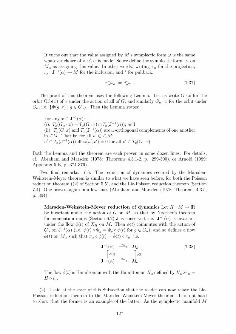
It turns out that the value assigned by M ’s symplectic form ω is the samewhatever choice of x, u′, v′ is made. So we define the symplectic form ωα onMα as assigning this value. In other words: writing πα for the projection,iα : J−1(α) →M for the inclusion, and ∗ for pullback:

π∗αωα = i∗αω . (7.37)

The proof of this theorem uses the following Lemma. Let us write G · x for theorbit Orb(x) of x under the action of all of G, and similarly Gα · x for the orbit underGα, i.e. {Φ(g, x) | g ∈ Gα}. Then the Lemma states:

For any x ∈ J−1(α):—(i): Tx(Gα · x) = Tx(G · x) ∩ Tx(J−1(α)); and(ii): Tx(G ·x) and Tx(J

−1(α)) are ω-orthogonal complements of one anotherin TM . That is: for all u′ ∈ TxM :u′ ∈ Tx(J

−1(α)) iff ω(u′, v′) = 0 for all v′ ∈ Tx(G · x).

Both the Lemma and the theorem are each proven in some dozen lines. For details,cf. Abraham and Marsden (1978: Theorems 4.3.1-2, p. 299-300), or Arnold (1989:Appendix 5.B, p. 374-376).

Two final remarks. (1): The reduction of dynamics secured by the Marsden-Weinstein-Meyer theorem is similar to what we have seen before, for both the Poissonreduction theorem ((2) of Section 5.5), and the Lie-Poisson reduction theorem (Section7.4). One proves, again in a few lines (Abraham and Marsden (1978: Theorems 4.3.5,p. 304):

Marsden-Weinstein-Meyer reduction of dynamics Let H : M → IRbe invariant under the action of G on M , so that by Noether’s theoremfor momentum maps (Section 6.2) J is conserved, i.e. J−1(α) is invariantunder the flow φ(t) of XH on M . Then φ(t) commutes with the action ofGα on J−1(α) (i.e. φ(t) ◦ Φg = Φg ◦ φ(t) for g ∈ Gα), and so defines a flow

φ(t) on Mα such that πα ◦ φ(t) = φ(t) ◦ πα, i.e.

J−1(α)�⏐⏐φ(t)

J−1(α)

πα−→πα−→

Mα�⏐⏐φ(t)

Mα

(7.38)

The flow φ(t) is Hamiltonian with the Hamiltonian Hα defined by Hα◦πα =H ◦ iα.

(2): I said at the start of this Subsection that the reader can now relate the Lie-Poisson reduction theorem to the Marsden-Weinstein-Meyer theorem. It is not hardto show that the former is an example of the latter. As the symplectic manifold M

127

one takes T ∗G, acted on symplectically by the cotangent lift of left translation. So weknow (from (3) of Section 6.5.3) that JL := T ∗

eRg is an Ad∗-equivariant momentummap ... and so on: I leave this as an exercise for the reader! The answer is suppliedat Arnold (1989: 377, 321) and Abraham and Marsden (1978: 302). (Abraham andMarsden call it the ‘Kirillov-Kostant-Souriau theorem’.)

Suffice it to say here that this exercise gives another illustration of one of our centralthemes, that g∗’s symplectic leaves are the orbits of the co-adjoint representation. Forthe reduced phase space Mα is naturally identifiable with the co-adjoint orbit Orb(α)of α ∈ g∗, with the symplectic forms also naturally identified; (cf. also result (2) at theend of Section 5.4).

Acknowledgements:— I am grateful to audiences in Irvine, Oxford, Princeton andSanta Barbara; to several colleagues for encouragement; and to Gordon Belot, KlaasLandsman, David Wallace, and especially Graeme Segal, for very helpful, and patient!,conversations and correspondence.

8 References

R. Abraham and J. Marsden (1978), Foundations of Mechanics, second edition: Addison-Wesley.

V. Arnold (1973), Ordinary Differential Equations, MIT Press.

V. Arnold (1989), Mathematical Methods of Classical Mechanics, Springer, (secondedition).

J. Barbour and B. Bertotti (1982), ‘Mach’s principle and the structure of dynamicaltheories’, Proceedings of the Royal Society of London A 382, p. 295-306.

G. Belot (1999), ‘Relationism rehabilitated’, International Studies in Philosophy ofScience 13, p. 35-52.

G. Belot (2000), ‘Geometry and motion’, British Journal for the Philosophy ofScience 51, p. 561-596.

G. Belot (2001), ‘The principle of sufficient reason’, Journal of Philosophy 98, p.55-74.

G. Belot (2003), ‘Notes on symmetries’, in Brading and Castellani (ed.s) (2003),pp. 393-412.

G. Belot (2003a), ‘Symmetry and gauge freedom’, Studies in the History and Phi-losophy of Modern Physics 34, p. 189-225.

G. Belot (this volume).

G. Belot and J. Earman (2001), ‘Pre-Socratic quantum gravity’, in C. Callender andN. Huggett (ed.s) Physics meets Philosophy at the Planck Scale, Cambridge UniversityPress, pp. 213-255.

128

R. Bishop and S. Goldberg (1980), Tensor Analysis on Manifolds, New York: Dover.

J. Boudri (2002), What was Mechanical about Mechanics: the Concept of Forcebetween Metaphysics and Mechanics from Newton to Lagrange, Dordrecht: KluwerAcademic.

K. Brading and E. Castellani (ed.s) (2003), Symmetry in Physics, Cambridge Uni-versity Press.

K. Brading and E. Castellani (this volume).

J. Butterfield (2004), ‘Some Aspects of Modality in Analytical mechanics’, in For-mal Teleology and Causality, ed. M. Stoltzner, P. Weingartner, Paderborn: Mentis.Available at Los Alamos arXive: http://arxiv.org/abs/physics/0210081 ; and at Pitts-burgh archive: http://philsci-archive.pitt.edu/archive/00001192.

J. Butterfield (2004a), ‘Between Laws and Models: Some Philosophical Morals ofLagrangian Mechanics’; available at Los Alamos arXive: http://arxiv.org/abs/physics/0409030; and at Pittsburgh archive: http://philsci-archive.pitt.edu/archive/00001937/.

J. Butterfield (2005), ‘Between Laws and Models: Some Philosophical Morals ofHamiltonian Mechanics’, in preparation.

J. Butterfield (2006), ‘On Symmetry and Conserved Quantities in Classical Me-chanics’, forthcoming in a Festschrift for Jeffrey Bub, ed. W. Demopoulos and I.Pitowsky, Kluwer: University of Western Ontario Series in Philosophy of Science.available at Los Alamos arXive: http://arxiv.org/abs/physics/ ; and at Pittsburgharchive: http://philsci-archive.pitt.edu/archive/00002362/

R. Darling (1994), Differential Forms and Connections, Cambridge University Press.

M. Dickson (this volume).

E. Desloge (1982), Classical Mechanics, John Wiley.

J. Earman (2003), ‘Tracking down gauge: an ode to the constrained Hamiltonianformalism’, in Brading and Castellani (ed.s) (2003), pp. 140-162.

H. Goldstein (1950), Classical Mechanics, Addison-Wesley; (1966 third printing).

I. Grattan-Guinness (2000), ‘A sideways look at Hilbert’s twenty-three problems of1900’, Notices of the American Mathematical Society 47, p. 752-757.

I. Grattan-Guinness (2006), ‘Classical mechanics as a formal(ised) science’, in B.Loewe (ed.), Foundations of the Formal Sciences, Kluwer, to appear.

T. Hawkins (2000), Emergence of the Theory of Lie Groups: an essay in the historyof mathematics 1869-1926, New York: Springer.

M. Jammer (1957), Concepts of Force, Harvard University Press.

M. Jammer (1961), Concepts of Mass in Classical and Modern Physics, HarvardUniversity Press; republished by Dover in 1997.

M. Jammer (2000), Concepts of Mass in Contemporary Physics and Philosophy,

129

Princeton University Press.

O. Johns (2005), Analytical Mechanics for Relativity and Quantum Mechanics, Ox-ford University Press, forthcoming.

A. Kirillov (1976), Elements of the Theory of Representations, Grunlehren Math.Wiss., Springer-Verlag.

H. Kragh (1999), Quantum Generations, Princeton University Press.

N. Landsman (this volume), ‘Between Classical and Quantum’.

S. Lie (1890). Theorie der Transformationsgruppen: zweiter abschnitt, Leipzig:B.G.Teubner.

J. Lutzen (1995), Denouncing Forces; Geometrizing Mechanics: Hertz’s Principlesof Mechanics, Copenhagen University Mathematical Institute Preprint Series No 22.

J. Lutzen (2003), ‘Between rigor and applications: developments in the conceptof function in mathematical analysis’, in Cambridge History of Science, vol. 5: Themodern physical and mathematical sciences, ed. M.J. Nye, p. 468-487.

J. Lutzen (2005) Mechanistic Images in Geometric Form: Heinrich Hertz’s ’Prin-ciples of Mechanics’, Oxford University Press.

J. Marsden and T. Hughes (1982), Mathematical Foundations of Elasticity, Prentice-Hall; Dover 1994.

J. Marsden and T. Ratiu (1999), Introduction to Mechanics and Symmetry, secondedition: Springer-Verlag.

E. McMullin (1978), Newton on Matter and Activity, University of Notre DamePress.

I. Newton (1687), Principia: Mathematical Principles of Natural Philosophy, trans.I.B. Cohen and A. Whitman, Cambridge University Press (1999).

P. Olver (2000), Applications of Lie Groups to Differential Equations, second edi-tion: Springer-Verlag.

C. Rovelli (this volume), ‘Quantum Gravity’.

T. Ryckman (2005), The Reign of Relativity: Philosophy in Physics 1915-1925Oxford University Press.

S. Singer (2001), Symmetry in Mechanics: a Gentle Modern Introduction, Boston:Birkhauser.

E. Slovik (2002), Cartesian Spacetime: Descartes’ Physics and the Relational The-ory of Space and Motion, Dordrecht: Kluwer Academic.

M. Stoltzner (2003), ‘The Principle of Least Action as the Logical Empiricist’sShibboleth’, Studies in History and Philosophy of Modern Physics 34B, p. 285-318.

D. Wallace (2003), ‘Time-dependent Symmetries: the link between gauge symme-tries and indeterminism’, in Brading and Castellani (ed.s) (2003), pp. 163-173.

130