Steering Control Characteristics of Human Driver Coupled ... · i Steering Control Characteristics...
267
Steering Control Characteristics of Human Driver Coupled with an Articulated Commercial Vehicle Siavash Taheri A Thesis In the Department of Mechanical and Industrial Engineering Presented in Partial Fulfillment of the Requirements For the Degree of Doctor of Philosophy (Mechanical Engineering) at Concordia University Montreal, Quebec, Canada January 2014 © Siavash Taheri, 2014
-
Upload
duongnguyet -
Category
Documents
-
view
213 -
download
0
Transcript of Steering Control Characteristics of Human Driver Coupled ... · i Steering Control Characteristics...

i
Steering Control Characteristics of Human Driver Coupled
with an Articulated Commercial Vehicle
Siavash Taheri
A Thesis
In the Department
of
Mechanical and Industrial Engineering
Presented in Partial Fulfillment of the Requirements
For the Degree of
Doctor of Philosophy (Mechanical Engineering) at
Concordia University
Montreal, Quebec, Canada
January 2014
© Siavash Taheri, 2014

ii
CONCORDIA UNIVERSITY
School of Graduate Studies
This is to certify that the thesis prepared
By : Siavash Taheri
Entitled: Steering Control Characteristics of Human Driver Coupled With
an Articulated Commercial Vehicle
and submitted in partial fulfilment of the requirements for the degree of
DOCTOR OF PHILOSOPHY (Mechanical Engineering)
complies with the regulations of the University and meets the accepted standards with
respect to originality and quality.
Signed by the final examining committee:
Chair
Dr. H. Akbari
External Examiner
Dr. Y. He
External to program
Dr. V. Ramachandran
Examiner
Dr. Y. Zhang
Examiner
Dr. R. Sedaghati
Co-supervisor
Dr. S. Rakheja
Co-supervisor
Dr. H. Hong
Approved by
Dr. A. Dolatabadi, Graduate Program Director
Januavry 17, 2014 Dr. C. Trueman, Interim Dean
Faculty of Engineering & Computer Science

iii
ABSTRACT
Steering Control Characteristics of Human Driver Coupled With an Articulated
Commercial Vehicle
Siavash Taheri,
Concordia University, 2013
Road safety associated with vehicle operation is a complex function of dynamic
interactions between the driver, vehicle, road and the environment. Using different
motion perceptions, the driver performs as a controller to satisfy key guidance and
control requirements of the vehicle system. Considerable efforts have been made to
characterize cognitive behavior of the human drivers in the context of vehicle control.
The vast majority of the reported studies on driver-vehicle interactions focus on
automobile drivers with little or no considerations of the control limits of the human
driver. The human driver's control performance is perhaps of greater concern for
articulated vehicle combinations, which exhibit significantly lower stability limits. The
directional dynamic analyses of such vehicles, however, have been limited either to open-
loop steering and braking inputs or simplified path-following driver models. The primary
motivations for this dissertation thus arise from the need to characterize human driving
behavior coupled with articulated vehicles, and to identify essential human perceptions
for developments in effective driver-assist systems and driver-adaptive designs.
In this dissertation research, a number of reported driver models employing widely
different control strategies are reviewed and evaluated to identify the contributions of
different control strategies as well as the most effective error prediction and
compensation strategies for applications to heavy vehicles. A series of experiments was

iv
performed on a driving simulator to measure the steering and braking reaction times, and
steering and control actions of the drivers with varying driving experience at different
forward speeds. The measured data were analyzed and different regression models are
proposed to describe driver’s steering response time, peak steer angle and peak steer rate
as functions of driving experience and forward speed.
A two-stage preview driver model incorporating curved path geometry in addition to
essential human driver cognitive elements such as path preview/prediction, error
estimation, decision making and hand-arm dynamics, is proposed. The path preview of
the model is realized using near and far preview points on the roadway to simultaneously
maintain central lane position and vehicle orientation. The driver model is integrated to
yaw-plane models of a single-unit vehicle and an articulated vehicle. The coupled driver-
articulated vehicle model is studied to investigate the influences of variations in selected
vehicle design parameters and driving speed on the path tracking performance and
control characteristics of the human driver. The driver model parameters are subsequently
identified through minimization of a composite cost function of path and orientation
errors and target directional dynamic responses subject to limit constraints on the driver
control characteristics. The significance of enhancing driver's perception of vehicle
motion states on path tracking and control demands of the driver are then examined by
involving different motion cues for the driver. The results suggest that the proposed
model structure could serve as an effective tool to identify human control limits and to
determine the most effective motion feedback cues that could yield improved directional
dynamic performance and the control demands. The results are discussed so as to serve as
guidance towards developments in DAS technologies for future commercial vehicles.

v
Acknowledgments
My greatest appreciations to my parents and sisters for their constant support and love in
my endeavors throughout my lifetime.
I am sincerely grateful to my supervisors, Dr. Subhash Rakheja and Dr. Henry Hong for
initiating this research study as well as for their continued technical guidance and great
financial support during the completion of this thesis work.
I would also wish to acknowledge Dr. Pierro Hirsch, Mr. Stéphane Desrosiers and all my
friends who have volunteered their help and their great corporation during the
experimental stages of this work.
Last but not the least, I greatly thank all colleagues, faculty and staff at the department of
Mechanical and Industrial Engineering, and my dear friends, specially, Alireza Pazooki,
Roham Mactabi and Sining Liu, whose pure friendship has motivated my social and
academic life in Canada.

vi
LIST OF CONTENTS
List of Figures ........................................................................................................... xi
List of Tables ............................................................................................................ xviii
Nomenclature ............................................................................................................ xxiv
Abbreviations …………………………..………………………………………….. xxxi
CHAPTER 1
LITERATURE REVIEW AND SCOPE OF THE DISSERTATION
1.1 Introduction ....................................................................................................... 1
1.2 Review of Relevant Literature ......................................................................... 3
1.2.1 Perception and Prediction Process ............................................................ 5
1.2.2 Path Preview Process ................................................................................ 10
1.2.3 Decision Making Process .......................................................................... 15
1.2.4 Response/Reaction Time ........................................................................... 24
1.2.5 Limb Motion and Steering Dynamic ......................................................... 27
1.2.6 Performance Index and Identification of the Driver’s Control Parameters 30
1.3 Scope and Objective of the Dissertation ......................................................... 32
1.3.1 Objectives of the Dissertation Research .................................................... 34
1.3.2 Organization of the Dissertation ................................................................ 34
CHAPTER 2
RELATIVE PERFORMANCE ANALYSIS OF DRIVER MODELS
2.1 Introduction ....................................................................................................... 37
2.2 Yaw-Plane Vehicle Model ................................................................................ 38

vii
2.3 Mathematical Formulations of the Selected Driver Control Strategies ...... 43
2.3.1 Compensatory Driver Model ..................................................................... 44
2.3.2 Preview Compensatory Driver Model ....................................................... 47
2.3.3 Anticipatory/Compensatory Driver Model ................................................ 50
2.4 Identification of Driver Models Control Parameters .................................... 52
2.5 Sensitivity Analysis ........................................................................................... 54
2.6 Results and Discussions .................................................................................... 56
2.6.1 Influences of Variations in Vehicle Speed ................................................ 56
2.6.2 Influence of Variations in Vehicle Mass ................................................... 66
2.6.3 Influence of Understeer Coefficient of the Vehicle ................................... 72
2.7 Summary ........................................................................................................... 78
2.8 Conclusion ......................................................................................................... 79
CHAPTER 3
EXPERIMENTAL CHARACTERIZATION OF DRIVER CONTROL
PROPERTIES
3.1 Introduction ....................................................................................................... 81
3.2 Driving Simulator ............................................................................................. 82
3.2.1 Experiment Procedures ............................................................................. 83
3.2.2 Identification of Outliers ............................................................................ 85
3.3 Skill Classification ............................................................................................ 86
3.3.1 Maneuver Accomplishment ....................................................................... 87
3.3.2 Peak Steer Angle and Steer Rate ............................................................... 89
3.3.3 Steer Angle and Steer Rate Crest Factors ................................................. 93
3.3.4 Steering Profile Area ................................................................................. 96

viii
3.3.5 Mean and Peak Speed Deviations from the Target Speed ......................... 98
3.3.6 Summary of the Skill Classification .......................................................... 99
3.4 Measurement of the Braking and Steering Response Times ........................ 100
3.4.1 Abrupt Braking Maneuver ......................................................................... 101
3.4.2 Obstacle Avoidance Maneuver .................................................................. 102
3.5 Results and Discussions .................................................................................... 103
3.5.1 Braking Response Time ............................................................................. 103
3.5.2 Steering Response Time ............................................................................ 106
3.6 Characterization of Drivers’ Control Properties ........................................... 108
3.6.1 Peak Steer angle ........................................................................................ 109
3.6.2 Peak Steer Rate .......................................................................................... 111
3.6.3 Coupled Driver-Vehicle responses - Clear Visual Situation ..................... 113
3.6.4 Coupled Driver-Vehicle responses - Restricted Visual Situation .............. 115
3.7 Summary ........................................................................................................... 116
CHAPTER 4
DEVELOPMENT OF THE COUPLED DRIVER-VEHICLE MODEL
4.1 Introduction ....................................................................................................... 118
4.2 Yaw-Plane Vehicle Models ............................................................................... 119
4.3.1 Yaw-Plane Model of the Articulated Vehicle ........................................... 120
4.3 Formulation of the Two-Stage Preview Driver Model .................................. 123
4.3.1 Driver’s Perception and Prediction …….................................................... 123
4.3.2 Two-stage Preview and Parameters Estimations ....................................... 125
4.3.3 Decision Making Process .......................................................................... 130
4.4 Coupled Driver-Single-Unit Vehicle Model ................................................... 132

ix
4.4.1 The Generalized Performance Index ........................................................ 133
4.4.2 Validation of the Coupled Driver-Vehicle Model - Clear Visual Field ... 135
4.4.3 Validation of the Coupled Driver-Vehicle Model - Limited Visual Field 138
4.5 Coupled Driver-Articulated Vehicle Model ................................................... 142
4.6 Summary ........................................................................................................... 147
CHAPTER 5
IDENTIFICATION OF DRIVER’S CONTROL LIMITS
5.1 Introduction ....................................................................................................... 148
5.2 Identification of the Driver’s Control Parameters ........................................ 149
5.3 Sensitivity Analysis - Driver Model Parameters ............................................ 152
5.4 Sensitivity Analysis - Variations in Speed and Vehicle Design Parameters 155
5.5 Identification of Control Limits of the Driver ............................................... 159
5.5.1 Variations of the Forward Speed ............................................................... 160
5.5.2 Variations in Tractor Design Parameters ………....................................... 165
5.5.3 Variations in Semi-Trailer Design Parameters ……………...................... 173
5.6 Summary ........................................................................................................... 181
CHAPTER 6
IDENTIFICATION OF EFFECTIVE MOTION CUES PERCEPTION
6.1 Introduction ....................................................................................................... 183
6.2 Perception of Different Vehicle States by the Human Driver ...................... 184
6.3 Identification of Effective Motion Cues Perception ……………………….. 186
6.3.1 Influence of Additional Feedback Cues - High Speed Driving …............. 187
6.3.2 Influence of Additional Feedback Cues - Heavier Tractor Unit ………… 193

x
6.3.3 Influence of Additional Feedback Cues - Longer Tractor Unit …………. 196
6.3.4 Influence of Additional Feedback Cues - Higher Tractor Tandem Spread 198
6.3.5 Influence of Additional Feedback Cues - Heavier Trailer Unit ………… 200
6.3.6 Influence of Additional Feedback Cues - Longer Trailer Unit ………….. 203
6.3.7 Influence of Additional Feedback Cues - Higher Trailer Tandem Spread 205
6.4 Summary ........................................................................................................... 207
CHAPTER 7
CONCLUSIONS AND RECOMMENDATIONS
7.1 Highlights and Major Contributions of the Dissertation Research ............. 209
7.2 Conclusions ........................................................................................................ 211
7.3 Recommendations for Future Studies ............................................................ 213
REFERENCES …………………………………………………………............... 216
APENDIX A
A.1 Yaw-Plane Model of the Single-Track Articulated Vehicle ….………............. 229
A.2 Yaw-Plane Articulated Vehicle Model …………………………………...…... 211
A.3 Simulation Results of Tire Cornering and Aligning Properties ………...…….. 213

xi
LIST OF FIGURES
Figure 1.1: Overall structure of the coupled driver/vehicle system …………… 4
Figure 1.2: The dead-zone model used to describe perception threshold of the
human body sensory feedbacks …………………………………… 7
Figure 1.3: Prediction of vehicle motion at a future instant using first-order
and second-order prediction models ………………………………. 9
Figure 1.4: The compensatory driver model structure ………………………… 17
Figure 1.5: The anticipatory/compensatory driver model structure …………… 18
Figure 1.6: The preview compensatory structure involving the driver’s
preview and prediction ……………………………………………. 19
Figure 1.7: Estimation of the vehicle orientation deviation …………………… 20
Figure 1.8: Visual angle of the lead car in a forward speed control system …... 21
Figure 1.9: Basic components and schematic of neuromuscular system ……… 27
Figure 1.10: Limb motion dynamics coupled with the steering system dynamics 28
Figure 2.1: Two DoF yaw-plane model of a single-unit vehicle ……………… 39
Figure 2.2: Comparisons of directional responses of the yaw plane vehicle
model with the simulator measured data under a double lane-
change maneuver at 30 km/h ……………………………………… 40
Figure 2.3: Comparisons of directional responses of the yaw plane vehicle
model with the simulator measured data under a double lane-
change maneuver at 50 km/h ……………………………………… 41
Figure 2.4: Comparisons of directional responses of the yaw plane vehicle
model (solid line) with the simulator measured data (dashed line)
under a double lane-change maneuver at 70 km/h ………………... 42
Figure 2.5: The compensatory driver model employing lateral position
feedback …………………………………………………………… 46
Figure 2.6: The compensatory driver model employing lateral position and
orientation feedbacks ………………………………………………
47

xii
Figure 2.7: The preview compensatory model employing second-order path
prediction ………………………………………………………….. 48
Figure 2.8: The preview compensatory driver model employing ‘internal
vehicle model’ path prediction strategy …………………………... 49
Figure 2.9: The preview compensatory driver model employing multi-point
preview strategy …………………………………………………… 50
Figure 2.10: The preview compensatory driver model employing multi-point
preview strategy together with the muscular dynamic ……………. 51
Figure 2.11: The anticipatory/compensatory driver model structure proposed by
Donges …………………………………………………………….. 52
Figure 2.12: Comparisons of the lead time constant, lateral position gain
constant (log scale) and orientation gain constant of the selected
driver models during a double-lane change maneuver at three
different speeds ……………………………………………………. 57
Figure 2.13: Comparison of the lead time constant, lateral position gain
constant and orientation gain constant of selected driver models
during a double-lane change maneuver subject to variations in the
vehicle mass (speed= 20 m/s) ……………………………………... 67
Figure 2.14: Comparison of the lead time constant, lateral position gain
constant and orientation gain constant of selected driver models
subject to variations of understeer coefficient (speed= 20 m/s) …... 74
Figure 3.1: Open cabin of the limited-motion driving simulator ……………… 81
Figure 3.2: The standard slalom course used in the experiments ……………... 86
Figure 3.3: Correlations of number of hit or missed cones with the driving
experience during slalom maneuvers at 70 km/h …………………. 87
Figure 3.4: Correlations of mean peak steer angle, and r2 values and
variations in CoV when data corresponding to a certain subject
was removed during slalom maneuver slalom at 30 km/h, 50 km/h
and 70 km/h ……………………………………………………….. 90
Figure 3.5: Correlations of mean peak steer rate during slalom maneuvers at
30 km/h, 50 km/h and 70 km/h ...………………………………….. 91

xiii
Figure 3.6: Correlations of mean steer angle crest factor, mean steering rate
crest factor with the driving experience during slalom maneuvers
at three selected target speed 30, 50 and 70 km/h ………………... 94
Figure 3.7: Steering profile of the driver, steering profile area, indicated by the
grey-shaded area …………………………………………………... 95
Figure 3.8: Correlations of mean steering profile area with the driving
experience during slalom maneuvers at three target speeds ...…….. 96
Figure 3.9: Correlations of mean speed deviations and peak speed deviations
with the driving experience during slalom maneuvers at 70 km/h ... 98
Figure 3.10: Braking response time in an abrupt braking maneuver …………… 101
Figure 3.11: Steering response time observed during an obstacle avoidance
maneuver ………………………………………………………….. 102
Figure 3.12: Variations in mean perception-processing times, mean foot
movement time and mean overall brake response time with
forward speed ……………………………………………………... 104
Figure 3.13: Variations in mean perception-processing and movement time
with participants’ driving experience ……………………………... 104
Figure 3.14: Variations in the steering response time due to variations in the
forward speeds and driving experience …………………………… 106
Figure 3.15: Standard course of the double-lane change maneuver ……………. 108
Figure 3.16: Peak steer angle and peak steer rate as functions of the forward
speed and driving experience during double-lane change
maneuvers …………………………………………………………. 112
Figure 3.17: Comparisons of path tracking and steering responses of ‘average’
(solid line) and ‘experience’ (dashed line) drivers groups under a
double lane-change maneuver at different speeds: 30 km/h, 50
km/h and 70 km/h (clear visual situation) …………………………
113
Figure 3.18: Comparisons of mean path tracking and steering responses of
average (solid line) and experience (dashed line) drivers groups
under a double lane-change maneuver at different speeds: 30 km/h,
50 km/h and 70 km/h (limited visibility condition) ………………. 115

xiv
Figure 4.1: Three DoF yaw-plane model of the articulated vehicle …………... 121
Figure 4.2: Comparisons of directional responses of the single-track yaw-
plane vehicle model (dashed line) and the nonlinear yaw-plane
vehicle model (solid line) with the measured data (dotted line)
during a lane-change maneuver at a constant speed of 68.8 km/h ... 121
Figure 4.3: The structure of the proposed two-stage preview driver model …... 122
Figure 4.4: Estimation of the near and far preview points on a straight-line
roadway and a curved path ………………………………………... 126
Figure 4.5: Estimation of the lateral position error ……………………………. 128
Figure 4.6: The two-stage preview driver coupled with a single-unit vehicle
model ……………………………………………………………… 131
Figure 4.7: Variations in control parameters of the driver model during a
double lane-change maneuver at different speeds for ‘experienced’
and ‘average’ drivers (clear visual field) …………………………. 134
Figure 4.8: Comparisons of measured path tracking and steering responses
(solid line) with the model responses (dashed line) for the
‘average’ driver group under a double lane-change maneuver at
different speeds: 30, 50 and 70 km/h (clear visual field) …………. 136
Figure 4.9: Comparisons of measured path tracking and steering responses
(solid line) with the model responses (dashed line) for the
‘experienced’ driver group under a double lane-change maneuver
at different speeds: 30, 50 and 70 km/h (clear visual field) ………. 137
Figure 4.10: Variations in control parameters of the driver models during a
double lane-change maneuver at different speeds for ‘experienced’
and ‘average’ driver (limited visibility field) ……………………... 138
Figure 4.11: Comparisons of measured path tracking and steering responses
(solid line) with the model responses (dashed line) for the
‘average’ driver group under a double lane-change maneuver at
different speeds: 30, 50 and 70 km/h (limited visual field) ………..
140
Figure 4.12: Comparisons of measured path tracking and steering responses
(solid line) with the model responses (dashed line) for the
‘experienced’ driver group under a double lane-change maneuver
at different speeds: 30, 50 and 70 km/h (limited visual field) …….. 141

xv
Figure 4.13: The coupled baseline driver-articulated vehicle system (solid line)
and the additional perceived motion states of the vehicle (dashed
line) corresponding to structures 2 to 10 ……………………… 142
Figure 4.14: Comparisons of (a) path tracking response; and (b) front wheel
steer angle of the coupled driver-articulated vehicle model (solid
line) with the measured data (dashed line) during a lane-change
maneuver at a constant speed of 68.8 km/h ……………………….. 145
Figure 5.1: Schematic of a tractor and semi-trailer combination illustrating
geometric and inertial parameters of interest ……………………... 149
Figure 5.2: Variations in the optimization problem solutions corresponding to
three different sets of initial values: (a) lateral position and
orientation gains; (b) far and near preview times; and (c) lead and
lag time constants …………………………………………………. 151
Figure 5.3: Path coordinates of the tractor cg during an open-loop step-steer
maneuver at 100 km/h with 20% increase in selected geometric
and inertial parameters ……………………………………………. 157
Figure 5.4: Influence of variations in the forward speed on the driver control
parameters during a double lane-change maneuver (50, 80, 100
and 120 km/h) ……………………………………………………... 161
Figure 5.5: Influence of variations in the forward speed on: (a) path tracking
response; and (b) steer angle of the tractor unit during double lane-
change maneuvers ………………………………………………… 161
Figure 5.6: Path deviation and orientation error of the articulated vehicle ……. 162
Figure 5.7: Influence of variations in the tractor mass on the driver control
parameters during a double lane-change maneuver (speed=100
km/h) ……………………………………………………………… 165
Figure 5.8: Influence of variations in the tractor mass on: (a) path tracking
response; and (b) steer angle during a double lane-change
maneuver (speed=100 km/h) ……………………………………… 165
Figure 5.9: Influence of variations in the tractor wheelbase on the driver
control parameters during a double lane-change maneuver
(speed=100 km/h) …………………………………………………. 168

xvi
Figure 5.10: Influence of variations in the tractor wheelbase on: (a) path
tracking response; and (b) steer angle during a double lane-change
maneuver (speed=100 km/h) ……………………………………… 168
Figure 5.11: Influence of variations in the tractor axle spreads on the driver
control parameters during a double lane-change maneuver
(speed=100 km/h) …………………………………………………. 170
Figure 5.12: Influence of variations in the tractor axle spreads on: (a) path
tracking response; and (b) steer angle during a double lane-change
maneuver (speed=100 km/h) ……………………………………… 170
Figure 5.13: Influence of variations in the semi-trailer mass on the driver
control parameters during a double lane-change maneuver
(speed=100 km/h) …………………………………………………. 173
Figure 5.14: Influence of variations in the semi-trailer mass on: (a) path
tracking response; and (b) steer angle during a double lane-change
maneuver (speed=100 km/h) ……………………………………… 173
Figure 5.15: Influence of variations in the semi-trailer wheelbase on the driver
control parameters during a double lane-change maneuver
(speed=100 km/h) …………………………………………………. 176
Figure 5.16: Influence of variations in the semi-trailer wheelbase on: (a) path
tracking response; and (b) steer angle during a double lane-change
maneuver (speed=100 km/h) ……………………………………… 176
Figure 5.17: Influence of variations in the semi-trailer axle spreads on the
driver control parameters during a double lane-change maneuver
(speed=100 km/h) …………………………………………………. 178
Figure 5.18: Influence of variations in the semi-trailer axle spreads on: (a) path
tracking response; and (b) steer angle during a double lane-change
maneuver (speed=100 km/h) ……………………………………… 179
Figure 6.1: Influence of employing different combinations of feedback cues
on variations in the lag time constant (TI) at a constant speed of
120 km/h …………………………………………………………... 191
Figure A.1: Three DoF yaw-plane model of the single-track articulated vehicle 229
Figure A.2: Dimensional parameters of the yaw-plane articulated vehicle
model ……………………………………………………………… 233
xvii
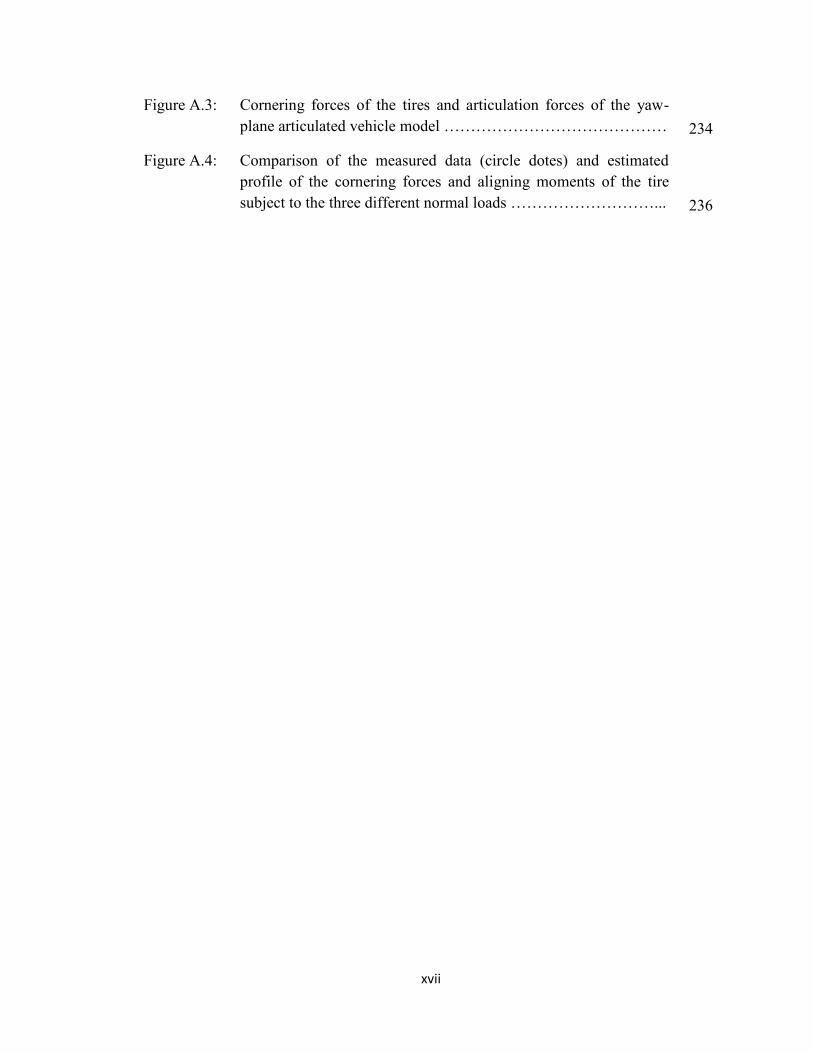
Figure A.3: Cornering forces of the tires and articulation forces of the yaw-
plane articulated vehicle model …………………………………… 234
Figure A.4: Comparison of the measured data (circle dotes) and estimated
profile of the cornering forces and aligning moments of the tire
subject to the three different normal loads ………………………... 236

xviii
LIST OF TABLES
Table 1.1: Different driver sensory feedbacks which is employed in the
reported studies ……………………………………………………. 6
Table 1.2: Summary of studies reporting objectively measured human driver
preview time ………………………………………………………. 13
Table 1.3: Summary of studies reporting indirectly identified preview time … 15
Table 1.4: Summary of reported driver model strategies related to the steering
behavior of the human driver ……………………………………... 22
Table 1.5: Studies reporting indirectly identified reaction times …………….. 25
Table 1.6: Summary of studies reported measured reaction times of human
drivers .…………………………………………………………….. 26
Table 1.7: Range of human driver’s control variables ……………………….. 31
Table 2.1: Simulation parameters of the single-unit vehicle model ………….. 39
Table 2.2: Summary of selected driver models ………………………………. 45
Table 2.3: Range of vehicle parameters and the nominal values employed in
sensitivity analysis ………………………………………………… 55
Table 2.4: Influences of variations in vehicle speed on the identified driver
model parameters and corresponding performance measures of the
selected driver-vehicle models ……………………………………. 58
Table 2.5: Sensitivity of directional responses and steering effort of selected
driver-vehicle models to variations in forward speed …………….. 63
Table 2.6: Sensitivity of total performance index and its constituents of the
selected driver-vehicle models to variations in forward speed …… 64
Table 2.7: Influences of variations in vehicle mass on the identified driver
model parameters and corresponding performance measures …….. 66
Table 2.8: Variation in peak directional responses of the selected driver
models to variations in the vehicle mass (speed=20 m/s) ………… 70
Table 2.9: Variation in total performance index and its constituents of the
selected driver models to variations in the vehicle mass (speed=20
m/s) ………………………………………………………………...
70

xix
Table 2.10: Influences of variations in understeer coefficient of the vehicle on
the identified driver model parameters and corresponding
performance measures …………………………………………….. 73
Table 2.11: Variation in the peak directional responses of the selected driver
models to changes in the understeer coefficient (speed=20 m/s) …. 76
Table 2.12: Variation in the total performance index and its constituents of the
selected driver models to changes in the understeer coefficient
(speed=20 m/s) ……………………………………………………. 77
Table 3.1: List of subject information ………………………………………... 82
Table 3.2: Total number of ‘hit’ or ‘missed’ cones during all trials of slalom
maneuvers …………………………………………………………. 87
Table 3.3: Peak front wheels steer angle measured during constant speed
slalom maneuvers …………………………………………………. 88
Table 3.4: Peak rate of steering input measured during constant speed slalom
maneuvers …………………………………………………………. 89
Table 3.5: Crest factor of the steer angle measured during slalom maneuvers.. 93
Table 3.6: Crest factor of rate of steering input measured during slalom
maneuvers …………………………………………………………. 94
Table 3.7: Steering profile area during slalom maneuvers …………………… 96
Table 3.8: Mean of ‘mean’ and ‘peak’ speed deviations during slalom
maneuvers …………………………………………………………. 98
Table 3.9: Summary of driving skill classification based upon the measures
considered during a slalom maneuvers ……………………………. 99
Table 3.10: Mean perception-processing and movement times of each
participant performing a straight-line braking maneuver at three
different speeds ……………………………………………………. 103
Table 3.11: Mean steering response time of each participant performing an
obstacle avoidance maneuver at three different speeds …………… 105
Table 3.12: Peak steer angle measured during the first two trials of constant
speed double-lane change maneuvers …………………………….. 109
Table 3.13: Peak rate of steering input measured during the first two trials of
constant speed double-lane change maneuvers …………………….
111

xx
Table 4.1: The steering system and the limb dynamic parameters, and the
identified control parameters of the coupled driver-articulated
model during a lane-change maneuver at 68.8 km/h ……………… 145
Table 5.1: Percentage change of the total performance index and its
constituents with variations in the driver model parameters ……… 153
Table 5.2: Range of vehicle parameters and the nominal values employed in
sensitivity analysis ………………………………………………… 155
Table 5.3: Percent changes in peak directional responses of the articulated
vehicle with 20% increase in the selected parameters …………….. 158
Table 5.4: Influence of variations in the forward speed of the vehicle on peak
errors in path tracking measures tracking responses of the driver-
vehicle system …………………………………………………….. 163
Table 5.5: Influence of variations in the forward speed of the vehicle on peak
directional responses of the driver-vehicle system ………………... 163
Table 5.6: Influence of variations in the tractor mass on peak errors in path
tracking measures of the driver-vehicle system (speed=100 km/h).. 166
Table 5.7: Influence of variations in tractor mass on peak directional
responses of the driver-vehicle system (speed=100 km/h) ……….. 166
Table 5.8: Influence of variations in tractor wheelbase on peak errors in path
tracking measures of the driver-vehicle system (speed=100 km/h).. 169
Table 5.9: Influence of variations in tractor wheelbase on peak directional
responses of the driver-vehicle system (speed=100 km/h) ……….. 169
Table 5.10: Influence of variations in tractor axle spreads on peak errors in
path tracking measures of the driver-vehicle system (speed=100
km/h) ……………………………………………………………… 171
Table 5.11: Influence of variations in tractor axle spreads on peak directional
responses of the driver-vehicle system (speed=100 km/h) ……….. 171
Table 5.12: Influence of variations in semi-trailer mass on peak errors in path
tracking measures of the driver-vehicle system (speed=100 km/h).. 174
Table 5.13: Influence of variations in semi-trailer mass on peak directional
responses of the driver-vehicle system (speed=100 km/h) ……….. 174
Table 5.14: Influence of variations in semi-trailer wheelbase on peak errors in
path tracking measures of the driver-vehicle system (speed=100
km/h) ………………………………………………………………
177

xxi
Table 5.15: Influence of variations in semi-trailer wheelbase on peak
directional responses of the driver-vehicle system (speed=100
km/h) ……………………………………………………………… 177
Table 5.16: Influence of variations in semi-trailer axle spread on peak errors in
path tracking measures of the driver-vehicle system (speed=100
km/h) ……………………………………………………………… 179
Table 5.17: Influence of variations in semi-trailer axle spread on peak
directional responses of the driver-vehicle system (speed=100
km/h) ……………………………………………………………… 180
Table 5.18: Influences of variations in the forward speed and vehicle design
parameters on path tracking performance and steering response of
the driver ………………………………………………………….. 181
Table 6.1: The proposed driver model structures employing driver’s
perceptions of different motion cue ………………………………. 184
Table 6.2: Range of human driver’s control parameters ……………………... 186
Table 6.3: Variations in the total performance index and its constituents by
considering different driver model structures considering nominal
vehicle parameters at a constant speed of 100 km/h ……………… 187
Table 6.4: Relative changes in path tracking and directional response
measures of the coupled driver-vehicle system integrating different
feedback cues compared to those obtained from the baseline model
(structure 1) considering nominal vehicle parameters at constant
speed of 100 km/h ………………………………………………… 188
Table 6.5: Variations in the total performance index and its constituents by
considering different driver model structures considering nominal
vehicle parameters at a constant speed of 120 km/h ……………… 189
Table 6.6: Relative changes in path tracking and directional response
measures of the coupled driver-vehicle system integrating different
feedback cues compared to those obtained from the baseline model
(structure 1) considering nominal vehicle parameters at a constant
speed of 120 km/h ………………………………………………… 190
Table 6.7: Variations in the total performance index and its constituents by
considering different driver model structures for a heavier tractor
unit (100 km/h) …………………………………………………… 192
Table 6.8: Relative changes in path tracking and directional response
measures of the coupled driver-vehicle system with respect to
those obtained from the baseline model (structure 1) considering
different feedback cues for a heavier tractor unit (100 km/h) …….. 194
xxii
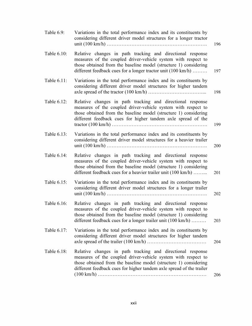
Table 6.9: Variations in the total performance index and its constituents by
considering different driver model structures for a longer tractor
unit (100 km/h) ……………………………………………………. 196
Table 6.10: Relative changes in path tracking and directional response
measures of the coupled driver-vehicle system with respect to
those obtained from the baseline model (structure 1) considering
different feedback cues for a longer tractor unit (100 km/h) ……… 197
Table 6.11: Variations in the total performance index and its constituents by
considering different driver model structures for higher tandem
axle spread of the tractor (100 km/h) ……………………………... 198
Table 6.12: Relative changes in path tracking and directional response
measures of the coupled driver-vehicle system with respect to
those obtained from the baseline model (structure 1) considering
different feedback cues for higher tandem axle spread of the
tractor (100 km/h) …………………………………………………. 199
Table 6.13: Variations in the total performance index and its constituents by
considering different driver model structures for a heavier trailer
unit (100 km/h) ……………………………………………………. 200
Table 6.14: Relative changes in path tracking and directional response
measures of the coupled driver-vehicle system with respect to
those obtained from the baseline model (structure 1) considering
different feedback cues for a heavier trailer unit (100 km/h) ……... 201
Table 6.15: Variations in the total performance index and its constituents by
considering different driver model structures for a longer trailer
unit (100 km/h) ……………………………………………………. 202
Table 6.16: Relative changes in path tracking and directional response
measures of the coupled driver-vehicle system with respect to
those obtained from the baseline model (structure 1) considering
different feedback cues for a longer trailer unit (100 km/h) ……… 203
Table 6.17: Variations in the total performance index and its constituents by
considering different driver model structures for higher tandem
axle spread of the trailer (100 km/h) ……………………………… 204
Table 6.18: Relative changes in path tracking and directional response
measures of the coupled driver-vehicle system with respect to
those obtained from the baseline model (structure 1) considering
different feedback cues for higher tandem axle spread of the trailer
(100 km/h) …………………………………………………………
206

xxiii
Table 6.19: The most effective combinations of feedback cues to improve the
path deviation, steering effort and the total performance index of
the coupled driver-vehicle system ………………………………… 207
Table A.1: Geometric and Inertial parameters of the selected articulated
vehicle combination ………………………………………..……… 234

xxiv
NOMENCLATURE
SYMBOL DESCRIPTION
a Longitudinal distance of the front axle from the cg of the single-unit
vehicle, m
Longitudinal distance from kth
axle to the center of gravity of the
associated unit (k=1,2,3,4,5), m
Lateral acceleration of the single-unit vehicle, m/s2
Lateral acceleration of unit for the articulated vehicle combinations ( =1
for the tractor and =2 for the semi-trailer unit), m/s2
Maximum allowable lateral acceleration of the vehicle ( =1 for the single-
unit vehicle, and =2 for the articulated vehicle), m/s2
[ ] State matrix of the states-space model of the vehicle ( =1 for the single-
unit vehicle, and =2 for the articulated vehicle)
b Longitudinal distance of the rear axle from the cg of the single-unit
vehicle, m
Damping coefficient of the reflex system, N.m.s/rad
Damping coefficient of the drivers’ hand-arm system, N.m.s/rad
Damping coefficient of the steering system, N.m.s/rad
[ ] Input matrix of the states-space model of the vehicle ( =1 for the single-
unit vehicle, and =2 for the articulated vehicle)
Longitudinal distance between the articulation joint and the center of
gravity of unit ( =1 for the tractor and =2 for the semi-trailer unit), m
C Curvatures of the predicted coordinate of the vehicle trajectory, 1/m
Cd Instantaneous path curvature, 1/m
Cd,Tp Curvature of the previewed path at a future instant Tp, 1/m
Ce Instantaneous path curvature error, 1/m
Cornering stiffness of tires mounted on kth
axle of the articulated vehicle
(k=1,2,3,4,5), N/rad
Longitudinal stiffness of tires mounted on kth
axle of the articulated
vehicle (k=1,2,3,4,5), N

xxv
Crest factor of the steer angle
Crest factor of the rate of steering input
Dual tire spacing, m
Preview distance of the driver, m
and Near and Far preview distances, respectively
Cornering forces acting on the front and rear tires of the single-unit
vehicle, respectively, N
Fyk Cornering force of the kth
axle tires for the single-track articulated vehicle
(k=1,2,3,4,5), N
Fyki Cornering force of the ith
tire on axle k for the articulated vehicle (i=1,2
for k=1; i=1,2,3,4 for k=2,3,4,5), N
Normal load on the tire corresponding to kth
axle for the single-track
articulated vehicle (k=1,2,3,4,5), N
Normal load on the ith
tire on axle k for the articulated vehicle (i=1,2 for
k=1; i=1,2,3,4 for k=2,3,4,5), N
FXA and FYA Longitudinal and lateral forces at the articulation point, respectively, N
Steering ratio of the vehicle steering system
Izz Yaw moment of inertia of the single-unit vehicle, kg.m/sec2
Izzj Yaw moment of inertia of the unit j for articulated vehicle combinations
(j=1 for the tractor and j=2 for the semi-trailer unit), kg.m/sec2
The inertia of the drivers’ hand-arm system
The inertia of the steering system
Generalized performance index, summation of all indices
Weighted mean squared lateral position error of the vehicle
Weighted mean squared orientation error of the vehicle
Weighted mean squared steer angle of the human driver
Weighted mean squared steer rate of the human driver
Weighted mean squared lateral acceleration of the single-unit vehicle

xxvi
Weighted mean squared lateral acceleration of unit j for the articulated
vehicle combinations (j=1 for the tractor and j=2 for the semi-trailer unit)
Weighted mean squared yaw rate of the single-unit vehicle
Weighted mean squared yaw rate of unit j for the articulated vehicle
combinations (j=1 for the tractor and j=2 for the semi-trailer unit)
Weighted mean squared articulation rate for the articulated vehicle
combinations
The stiffness of the drivers’ hand-arm system, Nm/rad
The stiffness constants of the reflex system, Nm/rad
The stiffness of the steering system, Nm/rad
Curvature error compensatory gain, rad.m
Ky Lateral position error compensatory gain, rad/m
Orientation error compensatory gain, rad/rad
Proportional compensatory actions of the driver with respect to the
estimated path deviation (i=1) and orientation error (i=2) of the tractor
unit, and the selected perceived motion states of both the tractor and the
semi-trailer units, (i=3 to 7).
m Mass of the single-unit vehicle, kg
mj Mass of unit j for articulated vehicle combinations (j=1 for the tractor and
j=2 for the semi-trailer unit), kg.m/sec2
and Aligning moment acting on the front and rear tires of the single-unit
vehicle, respectively, N.m
Mk Aligning moment of the kth
axle tires for the single-track articulated
vehicle combinations (k=1,2,3,4,5), N.m
Mki Aligning moment of the ith
tire on axle k for the articulated vehicle
combinations (i=1,2 for k=1; i=1,2,3,4 for k=2,3,4,5), N.m
MDTk Dual tire moment of the kth
axle tires for the single-track articulated
vehicle combinations (k=1,2,3,4,5), N.m
r Yaw rate of the single-unit vehicle, rad/s
Yaw rate of unit j for the articulated vehicle combinations (j=1 for the
tractor and j=2 for the semi-trailer unit), rad/s

xxvii
Maximum allowable yaw rate of the vehicle (l=1 for the single-unit
vehicle, and l=2 for articulated vehicle), rad/s
t Time, s
Pneumatic trail of tires on kth
axle for the articulated vehicle (k=1,2,3,4,5),
m
Preview time of the human driver, s
Tfb Torque feedback of the steering system, N.m
TL Lead time constant, s
Lead time constant of the driver corresponding to the orientation error of
the vehicle, s
Lead time constant of the driver corresponding to the lateral position error
of the vehicle, s
TI Lag time constant, s
Lag time constant of the driver corresponding to the orientation error of
the vehicle, s
Lag time constant of the driver corresponding to the lateral position error
of the vehicle, s
Lag time of the neuromuscular system, s
and Near and Far preview times, respectively, s
Input vector of the state-space model of the vehicle
Longitudinal velocity of the vehicle in the vehicle-fixed coordinate (xy),
m/s
Longitudinal velocity of unit j for the articulated vehicle combinations
(j=1 for the tractor and j=2 for the semi-trailer unit) in the vehicle-fixed
coordinate, m/s
Lateral velocity of the vehicle in the vehicle-fixed coordinate (xy), m/s
Lateral velocity of unit j for the articulated vehicle combinations (j=1 for
the tractor and j=2 for the semi-trailer unit) in the vehicle-fixed
coordinate, m/s
State vector of the state-space model of the vehicle
XD and YD Longitudinal and lateral coordinates of the driver’s seat in the global axis
system (XY), respectively, m

xxviii
Xg and Yg Longitudinal and lateral coordinates of the driver’s seat in the global axis
system (XY), respectively, m
XP and YP Longitudinal and lateral coordinates of the predicted position of the tractor
cg in the global axis system (XY), respectively, m
XN and YN Longitudinal and lateral coordinates of the near target point in the global
axis system (XY), respectively, m
XF and YF Longitudinal and lateral coordinates of the far target point in the global
axis system (XY), respectively, m
XT and YT Longitudinal and lateral coordinates of the tangent point in the global axis
system (XY), respectively, m
Instantaneous lateral position of the vehicle, m
Instantaneous lateral velocity of the vehicle in the global axis system
(XY), m/s
Instantaneous lateral acceleration of the vehicle in the global axis system
(XY), m/s2
Instantaneous lateral position error of the vehicle in the global axis system
(XY), m
Predicted lateral coordinates of the vehicle in the global axis system (XY),
m
Previewed path coordinates at a future instant Tp in the global axis system
(XY), m
Perceived path error between the previewed path and predicted
coordinates of the vehicle in the global axis system (XY), m
Maximum allowable lateral position error, m
Average side-slip angle developed at the tires mounted on kth
axle of the
unit ( =1 for tractor and 2 for semi-trailer unit), (k=1,2,3 for =1; k=4,5
for =2), rad
Orientation of the single-unit vehicle, rad
Orientation of unit j for the articulated vehicle combinations (j=1 for the
tractor and j=2 for the semi-trailer unit), rad
Visual angle of the sight point, rad
Instantaneous orientation of the desired path, rad

xxix
Ψe Instantaneous orientation error, rad
Maximum allowable orientation error, rad
Visual angle of the predicted path, rad
Roll angle of the vehicle, rad
Φ Human driver’s overall visual field, rad
( ) State-transition matrix
Steering angle command of the human driver, rad
Vehicle’s front wheels steering angle, rad
Human driver steering wheel angle, rad
Peak steer angle during double lane-change maneuver, rad
Peak steer rate during double lane-change maneuver, rad/s
Peak steer angle in accordance with the known drivers’ limits, rad
Peak steer rate in accordance with the known drivers’ limits, rad/s
Deviation of the average speed from the target speed, m/s
Peak difference between the instantaneous speed and the average speed,
m/s
Overall braking response time of the human driver, s
Overall steering response time of the human driver, s
Processing delay time of the human driver, s
The transport lag in sending messages to and from the spinal cord, s
Perception delay time of the driver, s
Movement delay time, s
The damping ratio of the combined manipulator and the limb muscles
The natural frequency of the combined manipulator and the limb muscles,
rad/s
The cut-off frequency of the reflex system, rad/s
Articulation angle of the articulated vehicle combination, rad

xxx
Articulation rate of the articulated vehicle combination, rad/s
Maximum allowable articulation rate for the articulated vehicle
combinations, rad/s

xxxi
ABBREVIATIONS
ANOVA Analysis of variance
ADAS Active driver assist system
BACs Blood alcohol concentration
CCD Charge-coupled device
DAS Driver-assist system
DoF Degree of freedom
EMG Electromyography
MOU Memorandum of understanding

1
1 CHAPTER 1
LITERATURE REVIEW AND SCOPE OF THE DISSERTATION
1.1 Introduction
The directional control performance of road vehicles is primarily influenced by the
driver's control actions that arise from the driver's interactions with the vehicle, road and
the environment. The main objective of the driver is to satisfy the control and guidance
requirements of the driving task in a controlled and stable manner. Generally, these
would include reducing the path tracking error to a permissible threshold level, and
rejection of the environmental and road disturbances. The human driver is known to
exhibit limited control performance, particularly in situations demanding critical steering
maneuvers, which has been associated with unsafe vehicle operations and vast majority
of the road accidents [1]. During 2009, nearly 5.5 million motor vehicle crashes leading
to nearly 1.5 million injuries and 31,000 fatalities were reported in the US alone [2,3].
The reported highway accident data suggest that nearly 90% of such accidents are
primarily attributable to errors related to drivers' perception of risk situations, decision
making process and control actions [4]. Although the number of crashes have been
steadily declining in recent years, the costs of such accidents associated with fatalities,
compensation and loss of quality of life remain unacceptable. Considerable efforts have
thus been made to characterize cognitive behavior of human drivers in the context of
vehicle control [5-7]. A number of experimental and analytical studies have attempted to
characterize human control and driving behavior, over the past five decades. These
studies generally focus on identifications of essential control characteristics of the driver

2
through objective measurements and formulations of mathematical models that describe
the driver as a controller considering the human perception, prediction, preview and
compensation abilities [7-9]. The resulting models have been applied for: (i)
identification of control characteristics of the human driver coupled with a vehicle, e.g.,
[10-12]; (ii) identification of control limits of the human driver, e.g., [13,14]; (iii)
developments in driver-adaptive vehicle designs, e.g., [15,16]; and (iv) developments in
effective driver-assist systems (DAS), e.g., [17,18]. The reported coupled driver-vehicle
models range from single-feedback closed-loop lateral position control models, e.g.,
[10,19], to multi-loop control models incorporating comprehensive sensory feedback
cues, e.g., [9,11,20,21]. Irrespective of the control structure, reported models generally
consider the driver as an ideal controller that can readily adjust its driving strategy to
adapt to a desired vehicle path with little or no considerations of control limits of the
human driver [9]. Thus, the model parameters, reported in such studies may be
considered valid only in the vicinity of the vehicle design and operating conditions
selected for identification of the driver model. The reported models, depending upon the
control strategies, may exhibit substantial path deviation and even instabilities under
higher operating speeds or emergency type of path change maneuvers. These may be in-
part attributed to the selected feedback cues that are integrated with different control
strategies.
It has been widely accepted that perception of the path information through visual
channel and vehicle motion prediction significantly influences the path tracking
performance and steering response of the coupled driver-vehicle system [22-24]. The
reported models, with only a few exceptions [11,25,26], however, have been developed

3
considering dynamics of automobiles only. The driver behavior characterization,
however, is far more vital for articulated commercial vehicles that exhibit substantially
different dynamics and lower control limits compared to automobiles.
In this dissertation research, a two-point preview strategy is used to develop a driver
model. The proposed model involves essential elements of the human driver, such as
perception, prediction, path preview, error estimation, decision making and hand-arm
system dynamics in conjunction with a directional dynamics of a single-unit as well as an
articulated freight vehicle. The driver model parameters are identified by minimizing a
composite performance index subject to constraints imposed by the human driver’s
control and compensation limits. Subsequently, the control demands on the driver are
evaluated through enhanced perception of different vehicle states so as to identify
secondary cues that could facilitate vehicle path tracking while limiting the control
demands. The vehicle states that help reduce path deviation could be utilized as
additional sensory feedbacks in a driver-assist system (DAS) for enhanced path tracking
performance of the coupled driver-vehicle system.
1.2 Review of Relevant Literature
A number of mathematical representations of the human driving behavior have evolved
since the 1950s. These models generally aim to describe human driving behavior in terms
of four essential elements, namely: (i) perception and prediction; (ii) preview; (iii)
decision making process; and (iv) limbs motions (Figure 1.1) [6,7,27]. Drivers’
perception of the instantaneous states of the vehicle help to predict the future vehicle
trajectory in a qualitative sense [22,28], while the roadway coordinates are previewed
through the visual field, which is described as the preview process. Using the previewed

4
path coordinates and predicted vehicle trajectory, the driver estimates the error of the
vehicle trajectory with respect to the desired roadway. The driver subsequently imparts
required compensatory control to minimize the tracking error subject to control
performance limits, response delays, muscular dynamics and the vehicle steering system
dynamics.
Actual
steering angle
Predicted
motion of the
vehicle
Performance
Limits of the
Human Driver
Muscular dynamic
and
Steering dynamic
Vehicle
Dynamic
Torque
feedback
Decision making process
Path error
estimation
Perception of the vehicle
motion with respect to
body fixed coordinate
Vehicle state
prediction
Perception/Prediction
Path Preview
through visual cues
Preview
Path error
compensation
Processing time
delay
Perceived
states of
the vehicle
Instantaneous
states of the
vehicle
Estimated error
Required
steering
angle
Hand and steering dynamicsSensory delay
and thresholds
Path information
Figure 1.1: Overall structure of the coupled driver/vehicle system
Early studies were mostly attempted to estimate the human control actions by
minimizing instantaneous perceived error between the vehicle trajectory and the desired
path coordinates, using simplified single-loop compensatory models. These models,
however, yield considerable path deviation, particularly under high speed directional
maneuvers [7,9]. It has been suggested that a coupled driver/vehicle model would exhibit
superior control performance through formulation of driver's preview ability and perhaps
involving additional sensory feedback [29,30]. A few earlier studies and the majority of
the recent studies, have thus employed involve driver's preview and multiple feedback
variables, so as to enhance the path tracking performance. Further, a number of studies
have been concerned with the role of hand-arm system and muscular dynamics. The

5
reported driver models employed widely different strategies to formulate these essential
components. In the following subsection each essential elements of a generalized driver
model will be described and relevant reported studies will be briefly reviewed and
discussed in terms of model formulations. The limitations of different control strategies
are further discussed in view of the driver control limits and vehicle path tracking
performance to build the essential knowledge and formulate the scope of the dissertation
research.
1.2.1 Perception and Prediction Process
It is established that the vehicle driver can sense instantaneous vehicle motion states
through its visual, vestibular and kinesthetic cues [29]. Perceived motion states of the
vehicle assist the driver to undertake the required steering control actions. A number of
studies are thus focused on identification and characterization of required sensory cues
related to human perception together with their mathematical descriptions [29,31]. The
reported studies invariably consider that the instantaneous coordinates and orientation of
the vehicle relative to its surroundings is perceived by the driver through visual sensory
cues, suggesting that visual aspects of driving are of the highest significance [29,31-33].
Experimental studies have suggested that without specific training, even high-skilled
drivers are unable to perform a good driving task in the absence of visual feedback [34].
It is also suggested that human driver can perceive linear and rotational accelerations as
well as rotational velocities of the vehicle in a qualitative manner through vestibular and
body-distributed kinesthetic cues [29]. The reported studies, however, mostly focus on
single-unit vehicles and employ lateral coordinate and heading angle of the vehicle as the
two primary cues, which can be more precisely perceived by the human driver. In case of

6
articulated vehicle combinations, it has been suggested that drivers’ perception of
secondary cues related to additional motion states of the vehicle could further assist the
driver to undertake the required steering control actions more effectively. These may
include articulation rate, lateral acceleration and yaw velocity of both the tractor and the
semi-trailer units. Table 1.1 summarizes the range of sensory feedbacks considered in
reported studies on human steering behavior, where the studies are identified by the lead
author alone.
Table 1.1: Different driver sensory feedbacks which is employed in the reported studies
First Author
Driver’s sensory cues
Lateral
position
Heading
angle
Lateral
velocity
Lateral
acceleration
Yaw
rate
Path
curvature
Roll
angle
Articulation
rate
Kondo (1985) ■
Weir (1968) ■ ■ ■ ■ ■
Yoshimoto (1969) ■
McRuer (1975) ■ ■
Donges (1978) ■ ■ ■
Hess (1980) ■
Reid (1981) ■ ■ ■
MacAdam (1981) ■
Garrot (1982) ■ ■
Legouis (1987) ■
Allen (1988) ■ ■
Hess (1989) ■ ■
Mojtahedzadeh(1993) ■
Mitschke (1993) ■
Horiuchi (2000) ■ ■
Sharp (2000) ■ ■
Yang (2002) ■ ■ ■ ■ ■ ■
Guo (2004) ■ ■ ■
Edelmann (2007) ■ ■
Ishio (2008) ■
Pick (2008) ■ ■ Menhour (2009) ■ ■ ■
Sentouh (2009) ■ ■ ■
The human perception of instantaneous vehicle states can be described considering
two essential characteristics: (i) perception delay time [5]; and (ii) a perception threshold

7
that relates to minimum value of a state that can be sensed by the human driver [32]. The
delay time to perceive vehicle states, denoted as the driver’s perception delay time ,
could vary from 0.1 to 0.2 depending upon the driver’s sensory channels and
environmental factors [1,29,33]. The magnitude of a vehicle state, however, must exceed
its threshold value to be detected by the human driver. The threshold values, however,
vary for different sensory channels. For instance, it has been reported that human can
detect linear acceleration exceeding 0.06 m/s2 through the vestibular system [29,33,35-
38]. The perception threshold of the human driver can be mathematically expressed by a
dead-zone operator (Figure 1.2), such that [29]:
( ) {
{ }
{ }
(1.1)
where and are instantaneous and perceived motion states, and is the perceptive
threshold of vehicle state j (j=1,…, n); n being the number of motion states to be
perceived.
Motion states
information
Perc
eiv
ed
info
rmati
on
Dead zone
Tj>0
Tj<0
Sj
Ij
Figure 1.2: The dead-zone model used to describe perception threshold of the human
body sensory feedbacks

8
The human driver continually predicts vehicle coordinates at a future instant in a
qualitative sense on the basis of the perceived information such as heading angle, forward
speed, lateral acceleration and lateral coordinates of the vehicle. The driver subsequently
undertakes a control or corrective action on the basis of anticipated deviations between
the predicted and previewed paths [28,39,40]. A number of attempts have been made to
characterize the driver prediction capability through different prediction models [41,42].
Assuming a constant lateral velocity and heading angle of the vehicle within the preview
interval, a first-order prediction model is used to estimate the future lateral coordinate of
the vehicle, such that [41]:
( ) ( ) ( ) (1.2)
where ( ) is the predicted lateral coordinate of the vehicle at a future instant in
the global X-Y frame, as shown in Figure 1.3(a), represent time, and ( ), and
are, respectively the instantaneous lateral position, orientation and forward speed of the
vehicle. The preview distance in the figure is indicated by Dp=Tpvx. The term ( )
can be approximated by the instantaneous lateral velocity of the vehicle, ( ), in the
global X-Y frame, such that:
( ) ( ) ( ) (1.3)
Owing to the constant lateral velocity assumption within the preview interval, this
approach is considered accurate for predicting first order trajectories. Alternatively, the
second-order prediction model considering constant lateral acceleration of the vehicle
within the preview interval has been formulated, as (Figure 1.3b) [42]:
( ) ( ) ( )
( ) (1.4)

9
It is suggested that the second-order prediction yield improved predictability of the
vehicle motion compared to the first-order model [8,42]. A third-order prediction model
has been also reported in a few studies. However, it has been shown that the third-order
prediction model is usually over-demanding and leads to directional instability of the
coupled driver-vehicle system [8].
X
Y
Predicted position
vx
vy
ΨY(t+TP)
Y(t)
X(t+TP)X(t)T
p vx sin
Ψ
Dp = Tpvx
X
Y
Predicted positionvx
Ψ
Y(t+TP)
Y(t)
X(t+TP)X(t)
vy
0 0
Figure 1.3: Prediction of vehicle motion at a future instant using (a) first-order prediction
model; and (b) second-order prediction model
A number of studies have employed a more elaborated formulation of the human
driver's prediction ability through the so-called ‘internal vehicle model’. These suggest
that the human drivers may employ prior knowledge of the vehicle response trends to
predict vehicle coordinates at a future instant [18,22,28]. A linear state-space model of
the vehicle has thus been proposed for determination of future coordinates of a vehicle,
such that [40]:
( ) [ ] ( ) [ ] ( ) (1.5)
where and are the state and input vectors of the state-space model of vehicle, and
[ ] and [ ] are respectively the state and input matrices for a single-unit vehicle. The
homogenous and non-homogenous solutions of the vehicle motion can be obtained from:
(a) (b)

10
( ) [ ( )] ( ) ∫ [ ( )][ ] ( )
(1.6)
where is the initial time. Assuming time invariant vehicle parameters, the state
transition matrix [ ( )] [ ] is estimated using the Taylor series approximation:
[ ] ∑([ ] )
(1.7)
Combining Eqs. (1.6) and (1.7), the predicted motion states of the vehicle at a future
instant are obtained as follow:
( ) (∑([ ] )
) ( ) (∑([ ] )
( )
) [ ] ( ) (1.8)
Using the above equation the predicted coordinates of the vehicle cg at a future
instance can be determined. The above formulation employs linear approximations of
the tire and vehicle dynamics and thus could yield considerable inaccuracies. A few
recent studies have attempted to incorporate driver experience and skill in order to
account for variations in the tire-vehicle characteristics under different driving
conditions, so as to enhance the accuracy of the linear state-space vehicle model [22,28].
1.2.2 Path Preview Process
Many theoretical and empirical studies have shown that human driver tends to
compensate for its perception/response delays through preview of future path information
[31,43,44]. This path preview process involves assessment of the lateral coordinate,
orientation and curvature of the desired roadway at a pre-set sight point, denoted as the
preview point [41,45]. The preview distance (DP), the distance from the preview point to
the driver’s position, is strongly influenced by the vehicle forward speed, maneuver

11
severity, path curvature and driver’s path preview strategy [41,44,46,47]. The preview
distance is generally expressed in terms of preview time (TP), which can account for the
speed effect assuming constant driving speed within the preview interval, which could
range from 0.5 to 9 s [7,11,18,48].
A number of experimental and analytical studies have been performed either in the
field or on driving simulators to identify ranges of drivers preview distances and preview
times under different driving situations. For instance, an experimental study [49], showed
that the optimum preview distance on straight path driving is 21 m at constant forward
speeds ranging from 30 to 50 km/h. The reported studies have employed two different
methods to characterize driver preview distance based on: (i) direct measurements; and
(ii) indirect identification.
Direct measurement method
The driver preview distances have been measured directly using three different
techniques: (i) the slit method; (ii) the sight-point camera; and (iii) eye movement
tracking. In the slit method the driver is asked to drive while seeing through a horizontal
slit placed in front of the driver's eyes. Under this condition the driver observes a certain
distance ahead of the road through the slit. The preview distance is then determined from
driver’s eye and slit position [41]. In this approach the driver's normal visual scene is
obstructed, which may affect human driving behavior, particularly at higher speeds
[50,51]. In the sight-point camera measurement technique, an aperture device is used to
restrict driver's field of vision, while the preview distance is estimated from the width of
the previewed path [52,53]. The use of this method has been limited since it requires
driver's effort to focus at the sight point through the aperture. In eye movement tracking

12
method, the driver uses a helmet equipped with a camera to record the road scene and a
charge-coupled device (CCD) camera to capture the pupil movement [31,47,54-56]. The
preview distance is then captured from the instantaneous change in pupil and road
orientation. These studies show two main characteristics of driver’s path preview: (i)
driver mainly looks at the tangent point on the inside edge of the bend during a cornering
maneuver [57-59]; and (ii) driver's head movement performs most of the required
movements to observe road information [57]. This approach, however, has limitations in
differentiating between the eye and the head movements, and contribution of the driver's
peripheral vision [60-62]. Table 1.2 lists some of the experimental studies on human
driver preview process to identify the preview time of the human driver, where the
studies are identified by the lead author alone. Wide variability in the reported values
may be attributable to driver-, vehicle- and environmental-related factors such as
differences in measurement methods, driving task, participants’ skill and vehicle speed.
An examination of the reported results, however, revealed a number of important and
consistent findings. For instance, a higher forward speed, generally, requires a longer
preview distance, which tends to enhance directional stability of the vehicle. Further, the
preview distance tends to decrease considerably with increase in path curvature [46].

13
Table 1.2: Summary of studies reporting objectively measured human driver preview time
Author Apparatus Method of
measurement
Velocity
(m/s)
Preview time
(s)
Number of
subjects†
Driving task Major finding(s)
Gordon (1966) Autombile Sight point camera 6 - 6.5 6.9 7(M) 3(F) Curve negotiation Preview time independent of speed.
Mclean (1973) Autombile Sight point camera 9 – 13.5 1.6 - 2.4 8(M) 2(F) Straight course Preview time independent of speed.
Kondo (1978)
Autombile Slit method 3 - 16.5 2 - 9 10 Straight course Preview time linearly increasing with
speed. Autombile Sight point camera 3 – 7.5 2 - 4 10 Curve negotiation
Reid (1981)
Autombile Eye movement
tracking 14 2 - 3.5 3 (M) Obtacle avoidance Average previw time: 2.6 s
Driving
simulator
Eye movement
tracking 14 1 - 3.5 3 (M) Obtacle avoidance Average previw time: 2.8 s
Driving
simulator
Indirect
identification 14 0.7 - 0.9 6 (M) Lane tracking Indirect identifcation by minimzing the
error between the response quantity and
the measured data. Driving
simulator
Indirect
identification 14 1.5 - 3.3 4 (M) Obtacle avoidance
Afonso (1993) Autombile Eye movement
tracking 11 - 22 1.6 - 2.5 20 Curve negotiation
Preview distance as a function of path
curvature and speed.
Experience drivers employ farther preview
distances. Land (1994) Autombile Slit method ~12 1 - 2 3 Curve negotiation Significance of the tangent point during
curve negotiation.
Land (1995) Driving
simulator Slit method 16.9
0.93 far
0.53 near 3 Curve negotiation
Effectivenss of two preview points at high
speeds.
Boer (1996) Driving
simulator
Indirect
identification 25 0.4 - 0.5 5 Curve negotiation
Significance of the tangent point during
curve negotiation.
Zwahlen (1997) Autombile Eye movement
tracking 23.5 0.5 - 1.8 11
Straight course
Driving behavior in low visibility
condition.
Wilkie (2003) Driving
simulator
Eye movement
tracking 8 1 - 2.5 6 Curve negotiation
Particiapants did not look toward the
tangent point of the bends at low speeds.
Billington (2010) Driving
simulator
Eye movement
tracking 8 1.5 7(M) 7(F) Curve negotiaton
Participants used the distant road edges to
improve their heading judgments. †
M- Male subjects; F - Female subjects

14
Indirect identification methods
Considering wide variability in the reported preview time, vast majority of studies have
relied on indirect identifications of the preview time for formulating the driver models.
The indirect method is, invariably, employs a coupled vehicle-driver model, where the
parameters identification techniques are applied to achieve minimal error between a
response quantity and the corresponding measured data [45,63-65]. Indirect identification
of the preview characteristics, however, necessitates a reliable driver model. The reported
studies have thus been limited to identification of the preview distances for particular set
of driver control measures and vehicle dynamic variables, and would be considered valid
only for certain driving situations. Considerable discrepancies among the reported results
are evident, which are attributed to variations in methodology used, driving conditions
and the objectives. Table 1.3 lists some of the reported studies that employ indirect
identification of preview characteristics together with the ranges of preview time.
The vast majority of the studies on human driving behavior have employed a single-
point preview ahead of the vehicle to obtain the required path information. A single-point
preview strategy, however, may lead to unsatisfactory path tracking performance and
instability, particularly under high speed directional maneuvers coupled with a relatively
short preview distance [66]. A human driver would exhibit superior control performance
when a preview of the entire roadway is available. Only a few studies have proposed
multi-point preview strategy for enhanced directional control performance of the driver
[15,18]. A multi-point preview strategy involves simultaneous preview of a number of
equally spaced target points for mapping of the required path information [15,67].
Further, it has been experimentally illustrated that novice drivers tend to use near preview

15
points of the desired path to obtain the required information, while drivers with relatively
higher driving skills tend to employ farther preview points [66]. Consequently, a concept
of weighted multi-point preview has been used in a few studies [18,66,68,69].
Measurements performed under restricted visual situations have shown that human
drivers observing only two segments of the roadway achieve improved path tracking
performance that is similar to that could be realized with entire roadway visibility
[31,56,70,71]. A two-point strategy is thus considered adequate for describing driver
preview opposed to the more complex multi-point approach. A few studies have
employed two-point preview strategy to develop coupled single-unit vehicle-driver
models [21,45,65,72,73], which suggest that only two target points ahead of the vehicle
are sufficient to obtain the roadway coordinates [34,45,56].
Table 1.3: Summary of studies reporting indirectly identified preview time
Author Forward speed
(m/s)
Preview time
(s) Description Control Strategy
Weir (1968) 26.8 5 Error minimzation Cross-over
Yoshimoto (1968) 10 - 30 2.2 - 3.5 Error minimzation Proportional
McRuer (1975) 26.8 2.7 Error minimzation Cross-over
Donges (1978) 8.3 - 16.6 1 - 1.3 Error minimzation Two-level
MacAdam (1981) 26.8 1.3 Error minimzation Optimal preview
Hess (1985) 30 0.2 Error minimzation Lead compensation
Mitschke (1993) 14 - 30 0.6 - 0.75 Based on vehicle design
parameters Two-level
Sharp (2000) 60 0.5 Error minimzation Multi-point previrw
Yang (2002) 27.7 1.51 - 2.88 Based on driving skill Multi-loop
compensatory
Guo (2004) 22 1.4 Error minimzation Preview-follower
Edelmann (2007) < 8 0.4 – 0.8 Based on vehicle design
parameters Two-level
1.2.3 Decision Making Process
The decision making process involves driver's control strategy to compensate for the
perceived error between the previewed path and predicted trajectory of the vehicle, which
may depend upon the driving task, driver's skill and various situational conditions

16
[11,22,29]. The reported driver’s control strategies can be grouped under four categories,
namely: (i) compensatory control strategy; (ii) anticipatory/compensatory strategy; (iii)
preview compensatory strategy; and (iv) forward speed control strategies. While the first
three categories focus on steering strategies under constant forward speed, the last group
of studies aim at longitudinal speed control models.
Compensatory Control Strategy
The compensatory strategy aims to track the desired path by minimizing instantaneous
lateral position error (Ye) between the perceived trajectory (Y) and the desired path (Yd),
as shown in Figure 1.4. The compensatory control strategy has been widely expressed by
the well-known crossover model [10], which implies that the driver undertakes
compensations to realize a stable and well-damped non-oscillatory vehicle response in
the vicinity of the crossover frequency, ranging from 2 to 4 rad/s [29,75]. This model
suggests that the dynamic response of the open-loop driver-vehicle system can be
described by a delay time and an integrator. The required model parameters are thus
determined in accordance with dynamic response of the vehicle. The crossover model
strategy exhibits good correlation with the measured data in immediate vicinity of the
gain crossover frequency but it can cause substantial tracking errors and a directional
instability at frequencies distant from the crossover frequency [7,76].
The vast majority of the reported compensatory models have employed instantaneous
lateral position of the vehicle as the main sensory feedback to the driver. This, however,
may lead to substantial tracking errors and a directional instability of the coupled driver-
vehicle system, particularly under emergency type of steering maneuvers [7,29,43]. It is
suggested that, the addition of the driver preview and/or driver’s secondary sensory

17
feedbacks helps realized stable vehicle response [20,29,30,77,78]. A consideration of
additional sensory feedbacks, such as heading angle of the vehicle, helps to enhance the
path tracking performance of the coupled driver-vehicle system [7,11,71,78]. A number
of studies have also considered the previewed path information attained from the human
driver's visual channel, which will be discussed in the following subsection.
δF Vehicle
dynamics
Decision making
process, H(s) Vehicle pathDesired path Front wheels
steering angle-
+
Y
Yd
Path error
estimation
Perception of
vehicle motion
YYe
Figure 1.4: The compensatory driver model structure
Anticipatory/Compensatory Control Strategy
It is suggested that skilled drivers can simultaneously employ open-loop anticipatory and
closed-loop compensatory strategies to satisfy the control and guidance requirements of a
driving task [12,21,45,65]. One of the earliest anticipatory/compensatory models was
proposed by Donges [45]. The two-level driver model generates: (i) an anticipatory
steering action δa based on perception of the future course of driving; and (ii) a
compensatory steering δc, as shown in Figure 1.5, to maintain instantaneous central lane
position. The anticipatory open-loop strategy, attained through a learning process, is
related to the predictive steering action of the driver, while the closed-loop compensatory
steering enhanced the path tracking performance of the coupled vehicle-driver system
[21,45,79].
The anticipatory control action is primarily obtained from the perceived path
curvature, Cd, considering single or multiple preview points, while the compensatory

18
steering is based on an instantaneous lateral position, orientation and curvature error.
Edelmann et al. [12] and Mitschke [65] have employed Donges' [45] two-level driver
model to stuyd the driver-vehicle lateral dynamics. These models, invariably, obtain the
previewd pah information on the basis of the previewed path curvature. However, it has
been experimentally shown that the human driver exhibit limited ability to estimate the
previewed path curvature with a reasonably good accuracy due to the so-called ‘illusive
curve phenomenon’, where the curvature of short-radius curves is mainly underestimated
[56,79,80].
Decision making process
+
+ Vehicle
dynamics-
+
Vehicle path
YCompensatory
control action
δF
Path error
estimation
Y
Yd
Anticipatory
control actionPreview
Desired
path
Cd Cd,Tp
Perception
Ye
δa
δc
Figure 1.5: The anticipatory/compensatory driver model structure
Preview Compensatory Control Strategy
The preview compensatory driver models consider both the preview and prediction
ability of the human driver to minimize the perceived path tracking error between
the previewed path information and predicted motion of the vehicle , as shown
in Figure 1.6 [20,30,40,]. One of the first preview compensatory models was introduced
by Kondo and Ajimine [41], which employed a proportional controller to minimize the
lateral position error between the preview path and the predicted vehicle trajectory using
a first order prediction model. Guo and Guan [8] demonstrated enhanced path tracking
performance of the vehicle using a preview-follower concept in conjunction with a

19
second order prediction model. The concept involves variations in the required model
parameters in accordance with the driver’s preview process P(s) and coupled driver-
vehicle system F(s), as shown in Figure 1.6. MacAdam [40] proposed a more elaborate
preview/prediction formulation incorporating a linear state-space internal vehicle model.
An optimal control approach was employed to minimize a performance index comprising
lateral position error between the previewed path coordinate and predicted trajectory of
the vehicle.
Vehicle
dynamicsDesired path
Preview
P(s) -
+
Vehicle path
Y
Prediction/Perception
Decsision
making process
Yd δF
Path error
estimation
YTp
Yd,TpYe,Tp
Coupled driver-vehicle system, F(s)
Figure 1.6: The preview compensatory structure involving the driver’s preview and
prediction
Considering the single-point preview strategy, Allen et al. [81] formulated a driver
model to compensate for the orientation error between the previewed and the predicted
path, which is defined as the visual angle, as shown in Figure 1.7 [81,82]. Steering
control action is then realized as a function of the visual angle of the sight point,
visual angle of the predicted path , lateral position error and vehicle heading angle
between the previewed and predicted paths of the vehicle:
(
)
(1.9)
where and are the preview distance and compensatory gain constant, respectively,
and represents the human driver steering response time.

20
Ye
Dp
Predicted trajectory
Desired path
Desired Path
Predicted point
Ψ
Ye/Dp
Ψc
Ψv
Previewed point
Figure 1.7: Estimation of the vehicle orientation deviation proposed by Allen et al. [81]
Some recent studies have employed a two-level control strategy using two parallel
closed-loop compensatory actions considering simualtaneous compensation of the
precieved errors associtaed with a far and a near preview point. It is suggested that the far
target point satisfies the guidance requirement of the driving task, while the near target
preview point minimizes the instantaneous path deviation and assures adequate
disturbance rejection [70,71]. Salvucci and Gray [79] proposed a driver model to
simultaneously generate steering action in response to the previewed path and to maintain
a central lane position. Similarly, Sentouh et al. [72] proposed a two-level driver model
employing two closed-loop compensatory control strategies to satisfy the path tracking
task. Reported studies have employed widely different methods to acheive minimal error
between the previewed and predicted paths [18,21,22,42,67,73]. Table 1.4 summarizes
the strategies employed in the reported studies, which are identified by the lead author
alone.
Forward Speed Control Driver Models
The vast majority of the reported driver models assume constant forward speed. The
human driver, however, tends to vary vehicle speed in order to maintain lane position in

21
response to vehicle motion and road/environmental condition. A few studies have
attempted to consider human driver's adaptation to the instantaneous vehicle responses
and road/environmental conditions through forward speed variations. It has been
recognized that human driver invariably adjusts the vehicle forward speed in order to
maintain safe levels of lateral acceleration during curve negotiation [83] and distance
with respect to a moving object ahead of the vehicle [84-86]. Savkoor and Ausejo [83]
proposed a curve negotiation driver model employing the previewed path curvature to
predict the future lateral acceleration of the vehicle, while the vehicle speed was adjusted
to a predetermined level of lateral acceleration. In a similar manner, Reymond et al. [87]
used human driver model to predict lateral path deviation and adjust the forward speed to
maintain a predetermined level of lateral position error. Forward speed control models
have also been proposed on the basis of relative velocity with respect to a lead vehicle,
which would be similar to the adaptive cruise control (ACC) concept [84], relative
position [85], and visual angle [86], as seen in Figure 1.8.
Visual angle
Figure 1.8: Visual angle of the lead car in a forward speed control system proposed by
Pipes [86]

22
Table 1.4: Summary of reported driver model strategies related to the steering behavior of the human driver
Author Control strategy Formulation of the decision making process Sensory cues Description
Iguchi (1959) Compensatory model PID controller Lateral position Neglects driver’s response time
McRuer
(1967) Compensatory model
Proportional compensatory gain and an integrator
Lateral position Consider the cross-over control
strategy
McRuer
(1970) Compensatory model Lead-lag controller Lateral position
Consider the cross-over control
strategy and a first-order lag to
formulate muscle dynamic
McRuer
(1975) Compensatory model
Proportional compensatory gain for lateral position
error and a lead controller for the heading error
Lateral position
and heading angle
Consider the cross-over control
strategy
Donges (1978) Anticipatory/Compensatory
model
Two-level controller: open-loop anticipatory for the
previewed curvature of the path and closed-loop
proportional compensatory gains for instantaneous
lateral position, heading angle and curvature errors
Lateral position,
heading angle and
curvature
Consider two-target points and
a pure time delay to formulate
driver’s response time.
Reid (1981) Preview compensatory
model Lead-lag controller
Lateral position,
heading angle and
curvature
Consider a pure time delay to
formulate driver’s response
time.
MacAdam
(1981)
Preview compensatory
model Linear Quadratic Riccati regulator (LQR) Lateral position
Consider a performance index
comprising the previewed path
deviation, and the internal
vehicle model to formulate
driver’s prediction process
Guo (1983) Preview compensatory
model Lead-lag controller
Lateral position
and heading angle
Consider a second-order
prediction model to formulate
driver’s prediction process
Allen (1988) Preview compensatory
model Proportional compensatory gain
Lateral position
and heading angle -
Mojtahedzadeh
(1993)
Preview compensatory
model Lead controller Lateral position
Incorporate neuromuscular
dynamic of human driver
Mitschke
(1993)
Anticipatory/Compensatory
model
Two-level controller: open-loop anticipatory for the
previewed curvature of the path; and a closed-loop
lead-lag controller for instantaneous curvature error
Curvature
Internal vehicle model to
formulate driver’s prediction
process

23
Table 1.4 (Cont.): Summary of reported driver model strategies related to the steering behavior of the human driver
Author Control strategy Formulation of the decision making process Sensory cues Description
Sharp (2000) Preview compensatory
model Proportional compensatory gain
Lateral position
and heading angle
Incorporate the instantaneous
heading error and lateral
deviation related to multiple
target points
Horiuchi
(2000) Compensatory model
A lead compensatory controller for the lateral position error
and a lead-lag controller for heading error
Lateral position
and heading angle
Consider a performance index
comprising the lateral position
error, steer angle and two lead
time constants
Yang (2002) Preview compensatory
model
Proportional compensatory gain
Lateral position
and orientation
errors, and lateral
acceleration, yaw
rate and roll angle
of the tractor and
the trailing units
The preview time and the
response time vary depending
upon driver's skill level.
Employing the constraint
minimization technique to
determine the model
parameters
Ungoren
(2005)
Preview compensatory
model Linear quadratic riccati regulator (LQR)
Lateral position
and heading angle
Consider a tunable parameter
to assign relative importance
of lateral position and heading
errors.
Consider a performance index
comprising the magnitude and
rate of path deviation
Edelmann
(2007)
Anticipatory/Compensatory
model
Two-level controller: open-loop anticipatory for the
preview path curvature; and compensatory lead-lag
controller for perceived lateral position error
Lateral position
and curvature -
Ishio (2008) Compensatory model Lead-Lag controller Lateral position
Considering a performance
index comprising the lateral
position error and lateral
velocity together with steer
angle and steer rate
Sentouh
(2009)
Anticipatory/Compensatory
model
Two-level controller: closed-loop proportional controller
related to the heading angle error for the far preview point;
and compensatory lead-lag controller related to the
perceived heading angle error for the near preview point;
Lateral position
and heading angle
Incorporates neuromuscular
dynamic

24
1.2.4 Response/Reaction Time
The human reactions to external stimuli, in-general, exhibit time delays depending upon
the decision-making abilities, depth of the required mental processing, awareness,
expectancy and neuromuscular dynamics [1,7]. Conceptually, the driver's reaction time
( ) may be decomposed into the perception-processing time and the movement time. The
perception-processing time defines the time interval between observing a stimulus and
initiation of a discernible muscular response [33,38,88].
The perception-processing time may be further divided into four distinct stages,
namely: (i) detection; (ii) identification; (iii) decision making; and (iv) response time
[89]. The initial detection stage involves interval where the driver develops a conscious
awareness of a sudden stimulus. In the identification stage, the driver acquires sufficient
information to identify the nature of the event. Following the detection and identification
of a stimulus, the driver undertakes the decision stage involving information processing
and desirable control actions such as steering or braking [1]. In the final stage, denoted as
the response stage, the control command is transmitted by the motor center of the brain to
appropriate muscles to carry out the required actions [90]. It is extremely complex to
quantify the time intervals associated with each stage. The overall perception-processing
time, however, is mostly related to the depth of the required mental processing, age,
awareness and expectancy of the stimuli, and may vary among the different receptors
[33,91-93].
Movement time defines the interval to perform the intended action by the driver,
which mostly depends on the muscles dynamic, age, blood alcohol concentration (BACs)
and fatigue [91,94-99]. In the context of human driving control actions, two basic

25
approaches have been reported to describe the movement time: (i) the simplified pure
time delay; and (ii) the dynamic responses of the limbs. The first approach describes the
muscle movement dynamic as a pure time delay which can be added to the perception-
processing time to obtain an overall reaction time of the human driver [1,100-108]. Only
a few studies have attempted to measure the perception-processing and movement times
of human drivers. These have reported widely varying perception-processing times,
ranging from 0.1 to 2.8 s, and movement times, ranging from 0.16 to 0.76 s. The
differences are attributable to widely different stimuli considered in the reported studies,
as seen in Table 1.6. Owing to complexities associated with measurements of reaction
times, the vast majority of reported driver models identify the driver reaction time
indirectly by minimizing the error between a response quantity and corresponding
measured data. Table 1.5 summarizes the studies reporting the perception-processing and
movement times or the overall reaction time, which are identified by the lead author
alone. In the second approach, the movement time is identified from the muscle/limb
reaction times considering different muscles dynamic models coupled with steering
system dynamic, which are summarized in the following subsection.
Table 1.5: Studies reporting indirectly identified reaction times
Author Perception-processing time
(s)
Movement time
(s)
Overall reaction time
(s)
McRuer (1965) - - 0. 1 - 0.55
Weir (1968) 0.2 0.1 -
Yoshimoto (1969) - - 0.3
Donges (1978) - - 0.4 - 0.8
Hess (1981) 0.15 0.2 to 0.4 -
Reid (1981) - - 0.2 - 0.5
MacAdam (1981) - - 0.2
Mojtahedzadeh (1993) 0.15 0.4 -
Horiuchi (2000) 0.1 0.1 -
Yang (2002) - - 0.1 - 0.25 - 0.35
Guo (2004) 0.4 0.2 -
Edelmann (2007) - - 0.2
Pick (2008) - - 0.16

26
Table 1.6: Summary of studies reported measured reaction times of human drivers
Author Response Method of
measurement
Velocity
(m/s)
Perception-response
time (s)
Movment time
(s)
Number of
subjects†
Stimulus Major finding(s)
Barrett (1968) Braking Driving
simulator ~11 0.8 - 1.1
† 11
Appearance
of pedestrian
Dominant braking response
compared to steering
Davies (1969) Braking Driving
simulator -
0.15† (leveled brake and gas pedals)
0.31† (unleveled brake and gas pedals)
10
visual
stimulus
(light)
50% improvement of the
movement time for the pedals at
equal level
Olson (1986) Braking Automobile 12 - 14 (Y)
1 > 1.0
(O) 1
> 1.0
(Y) 1
> 0.7
(O) 1
> 0.5
49 (Y) 1
15 (O)
1
Obstacle
avoidanc
The perception-response time is
1.6 s for 95th precentile
Hancock (1999) Braking Driving
simulator 9, 13.5 0.61
2† 0.93(d)
2† 10 Traffic light
Response time increases in the
presence of distraction
Lenne (1999) Braking Driving
simulator 22
Alcohol: 0.86 - 0.93†
Non alcohol: 0.80 - 0.86†
14 (M)
14 (F) Visual sign
Response time under 0.7 ml/kg
alcohol impairment
Warshawsky-
Livne (2002) Braking
Driving
simulator 25
0.32(a) 3 0.42(ua)
3
0.35(Y) 1
0.43(O) 1
0.19 (M)
0.16 (F)
36 (M)
36 (F)
visual
stimulus
(light)
Perception-processing time
increase by age but decrease
with alertness
Young (2007) Braking Driving
simulator 30
(NO)4 2.10-2.74
(EX)4
2.24-2.76
(NO) 4 0.58-0.74
(EX) 4 0.71-0.76
26 (M)
18 (F)
Lead car
failure
Reaction response time of driver
to decceleration of the lead
vehicle
Mehmood
(2009) Braking
Driving
simulator 25
1.32 (a) 3†
0.78 (ua) 3†
31 (M) Brake light of
the lead car
Reaction response time of driver
to decceleration of the lead
vehicle 1.39 (a) 3†
0.85 (ua) 3†
29 (F)
Summala (1981) Steering Automobile 16.5 1.5† 1326
Sudden
appearence of
an obstacle on
the roadside
Inititation of the vehicle lateral
movement used to determine the
response time including the
vehilce response delay
Summala (1981) Steering Automobile 16.5 2† 815
visual
stimulus
Steering response to onset of a
visual stimuli on a dark road
McGehee (2000) Steering
Automobile 20 1.67† 192
intersection-
incursion statistical equivalence between
driver's reaction time in both
studies Driving
simulator 20-25 1.64
†
60 (M)
60 (F)
intersection-
incursion †
Overall reaction time; (M) male subject; (F) female subjects
1. Young (Y) and old drivers (O); 2. Driving under a distraction (d); 3. Aware (a) and Unaware (ua) of road stimuli; 4. Novice (NO) and Expert (EX) drivers

27
1.2.5 Limb Motion and Steering Dynamic
The driver’s steering command transmitted to the vehicle steering system through the
limb motions in response to skeletal muscles activations, as indicated in Figure 1.1
[76,90,109]. The muscles are made up of muscle fibers and spindles, which are controlled
by motor neurons whose cell bodies lie in the spinal cord [110]. The α-motoneurons and
γ-motoneuron cause contractions of muscle fibers and spindles, respectively, through
releasing of a chemical agent in the muscle fibers and spindles [75,109]. The force
developed by contraction of the muscle spindles, however, is substantially smaller than
that caused by the muscle fibers [90,111]. The γ-motoneurons, however, determine the
desired length of the muscle. The muscle spindles thus serve as sensory receptors within
the muscle to provide the position and velocity feedback and generate an error signal
[90,112,113]. This error signal coupled with a transmission delay time subsequently
activates α-motoneurons which results in contraction of muscle fibers and thus the
activation force, as seen in Figure 1.9 [43,109,114].
Spindle ensemble
α-motoneuron
pool
Demanded
Force Muscle
dynamicsSpindle
Limb position
α-motoneuron
command
γ-motoneuron
command
Central
nervous
system γ-motoneuron
delays
α-motoneuron
delays+-
++
Figure 1.9: Basic components and schematic of neuromuscular system
Formulations of the human limb motions in a control task can be traced from early
aircraft-pilot studies. These have established that during a compensatory tracking task, the
pilot’s muscle dynamics can be described by a linear second-order dynamic system

28
[10,27]. McRuer et al. [113] suggested that the muscular dynamic response of the
combined limb and a manipulator system can be formulated by a third-order transfer
function, denoted as the ‘Precision Model’. This transfer function describes the combined
manipulator/muscular dynamic from the α-motoneuron command signal to limb position
in the following manner:
( )
( )( ) (1.10)
where and are the damping ratio and natural frequency of the combined
manipulator and the limb muscles, while the first-order function describes the
neuromuscular system lag ( ). The above model is considered valid when the pilot
operates a manipulator and may not be applicable for vehicle driving task [111,115-117].
A series of driving simulator studies have been conducted to simultaneously measure
the muscle activity using surface electromyography (EMG) and the force applied to the
steering wheel [115]. The measured data were used to characterize the limb motion
response as a function of both the muscles and the steering system dynamic. The study
proposed a limb motion model, as shown in Figure 1.10, considering the reference model
Rm(s), muscles reflex model Hm(s), and active muscle stiffness function Km(s) [67,90].
Demanded
TorqueDesired
steering angle
Gm(s)Hm(s)
Limb motion, L(s)
Torque feedback
+
- +
- δFδd
Rm(s)
+
Tfb
Km(s)
Figure 1.10: Limb motion dynamics coupled with the steering system dynamics proposed
by Pick and Cole [67]

29
The coupled muscles and steering dynamics function, Gm(s), is characterized
considering second-order muscular dynamics of the human hand-arm and the steering
system, as [67]:
( )
( ) ( ) ( ) (1.11)
where , and are the inertia, damping and stiffness of the drivers’ hand-arm
system, respectively, and , , and are inertia, damping, stiffness and steering
ratio of the steering system, respectively. The steering action of the driver also involves
estimation of the torque demand, which is estimated using the reference model function,
Rm(s), expressed as the steady-state inverse of Gm(s) [67,118]:
( )
(1.12)
The difference between the desired and the actual steering angle is subsequently
sensed by muscle spindles [67,112]. A first-order lead-lag model is used to describe the
muscles reflex property Hm(s), which generates a corrective torque so as to maintain the
spindle-sensed steering position as [110,115]:
( ) ( )
⁄ (1.13)
where and are the damping and stiffness constants of the reflex system,
respectively, is the cut-off frequency that describes the time delay between the muscle
activation and generation of the muscle torque, and is the transport lag in sending
messages to and from the spinal cord, which could range from 0.025 to 0.05 s [67]. It is
also established that the muscle activation and co-contraction may imply greater stiffness
of the driver’s arms [118,119]. An additional gain constant Kma is thus used to represent
increase in the muscle stiffness, which is described by the active stiffness function Km(s)

30
[67,90]. The overall transfer function L(s) relating the front-wheels steering to driver's
steering command of , as shown in Figure 1.10, is described considering the torque
feedback of the steering system, Tfb, as:
( ) ( )
( ) ( ) ( ) ( ) ( ) ( ) ( ) ( )
( ) ( ) ( ) (1.14)
A number of studies have experimentally assessed the influence of steering torque
feedback on path tracking performance of the vehicle driver, and concluded insignificant
effect of the steering torque feedback [120-122]. It has been suggested that the dynamic
behavior of the vehicle steering system can be effectively formulated considering the
correlation between the vehicle response and the steering wheel angle, which may be
taken as the steering gear ratio, [67,120,123]. The majority of the reported studies
thus neglect the torque feedback effect characteristics of steering dynamic. These studies
either consider a constant gain as the steering ratio or characterize the steering system as a
second-order system.
1.2.6 Performance Index and Identification of the Driver’s Control Parameters
The directional control performance of road vehicles and thus the road safety are
influenced by control actions of the human driver and directional responses of the vehicle
such as lateral position and orientation errors. The control characteristics of the human
driver have been mostly identified through minimization of a composite performance
index of selected response measures. The selected measures for automobiles have been
mostly limited to the lateral position error ( ) or orientation error ( ) or a combination
of the two [7,17,40,78]. This approach of identifying the driver control properties may
thus yield an idealized driver model, particularly when the control limits of the human

31
driver are not considered in the performance index minimization. The vast majority of the
driver models, with only few exceptions, do not consider the driver control limits in the
control parameters identification process. The reported driver models thus suggest widely
different driver control characteristics that may be considered applicable for particular
driving condition considered in individual studies. Table 1.7 summarizes the ranges of
commonly used driver control parameters such as preview time, lead and lag time
constant, and lateral position and orientation error compensatory gains [8,11,14,17,45].
These clearly show wide ranges of control parameters used in different studies. Only a
few studies have reported solution of the minimization problem subject to limit
constraints defining the practiced ranges of driver control characteristics [11].
Table 1.7: Range of human driver’s control variables
Control variables Unit Range
Preview time, Tp s 0.10 – 2.50
Lead time constant, TL s 0.05 – 3.00
Lag time constant, TI s 0.02 – 0.80
Lateral position error compensatory gain, Ky rad/m 1e-5 – 1.80
Orientation error compensatory gain , KΨ rad/rad 0.10 – 1.85
The reported vehicle driver models employ widely different control characteristics and
performance indices comprising the vehicle path and directional responses together with
some measures of demands imposed on drivers' effort. These include the maximum
steering angle and its rate, which has been related to the driving effort and drivers'
comfort [9,15,17]. Since the majority of the studies have focused on driver models
applicable to automobiles or two-axle vehicles, the widely used performance index of
lateral position and orientation errors alone would be justifiable. Such a performance
index, however, would be inadequate for heavy articulated vehicle combinations where

32
the driver perceives additional cues from the vehicle responses. Only few studies have
explored driver models for articulated vehicle combinations, which have suggested
significance of many additional vehicle responses [9,25]. These employ performance
indices comprising weighted function of lateral accelerations, yaw rates and roll angles of
the articulated vehicle units; articulation angle and articulation rate; and steer angle and
its rate. Yang et al. [16] proposed such a performance index, which was minimized upon
consideration of ranges of reported control limits of the human driver including preview
time, lead and lag time constants and compensation gains.
1.3 Scope and Objective of the Dissertation
From the literature review, it is apparent that the reported human driver models generally
consider the driver as an ideal controller that can readily adjust its driving strategy to
adapt to a desired vehicle path with little or no considerations of control limits of the
human driver. Furthermore, the vast majority of the reported studies on driver-vehicle
interactions focus on automobile drivers. The human driver's control performance is
perhaps of greater concern for articulated vehicle combinations, which exhibit
significantly lower control limits and may pose relatively greater highway safety risks
compared to automobiles. The directional dynamic analyses of such vehicles have been
limited either to open-loop steering and braking inputs or simplified path-following
driver models.
In the context of interactions between the human driver and articulated vehicles, only
a few studies have investigated the coupled driver-vehicle system responses. These
generally focus on characterization of driving control requirements through minimization
of lateral position error between center of mass (cg) of the tractor and the desired path

33
using a single-point preview strategy. A single point preview strategy, however, may lead
to unsatisfactory path tracking performance and instability, particularly under high speed
directional maneuvers coupled with a relatively short preview distance. Furthermore, the
assessments of active safety devices in the vast majority of the studies have been limited
to either open-loop simulations or in a closed loop simulations using simple driver
models. The contributions of the human driver's control limits to the vehicle stability
have been mostly ignored. It is thus desirable to develop more effective driver models for
articulated vehicles considering feasible ranges of human driver control limits and
multiple-point preview. Such a model could serve as an effective simulations tool for
assessing safety dynamics of the coupled driver-vehicle system and provide essential
guidance toward developments in driver-assist systems (DAS).
This dissertation research thus aims to develop a two-stage preview strategy, involving
a near- and a far-point preview simultaneously, to characterize steering control properties
of commercial vehicle drivers. The strategy includes a near and a far preview point
targets to describe the driver control of lateral path deviation and vehicle orientation. A
human driver model comprising path error compensation and dynamic motions of the
limb is subsequently formulated and integrated to a yaw-plane model of an articulated
vehicle. The coupled driver-vehicle model is analyzed under an evasive steering
maneuver to identify limiting values of the driver control parameters through
minimization of a generalized performance index comprising driver’s steering effort, path
deviations and selected vehicle states. The performance index is further analyzed to
identify relative contributions of different sensory feedbacks, which may provide
important guidance for designs of driver-assist systems (DAS).

34
1.3.1 Objectives of the Dissertation Research
This dissertation research aims to characterize human driving behavior when coupled
with an articulated commercial vehicle and development of a comprehensive closed-loop
driver/vehicle model for identifications of control performance limits of heavy vehicle
drivers. The specific goals of the proposed research are summarized below:
1. Characterize essential control properties of the human drivers through
measurement on a vehicle simulator;
2. Develop a two-stage preview driver model and integrate the model to an
articulated vehicle model for analysis of coupled driver-vehicle system responses
as functions of vehicle drivers and operating factors;
3. Identify the ranges of driver model parameters, more specifically the driver
control performance limits, through formulation and minimization of a composite
performance index;
4. Identify the relative significance of difference motion and visual cues and
formulate a concept in driver-assist system (DAS) as additional sensory feedbacks
in order to enhance path tracking performance of the coupled driver-vehicle
system.
1.3.2 Organization of the Dissertation
This dissertation research is organized into six chapters, including a literature review
chapter (Chapter 1). In the initial chapter, the reported studies relevant to human driving
cognitive behaviors, sensory feedbacks and driver model structures, are reviewed to build
essential knowledge on methodologies for characterization of human driver and for
developing directional pursuit-compensatory driver model. The scope and objectives of
the dissertation research are also summarized.
In the second chapter, a number of reported driver models are selected and integrated
with a single-unit vehicle model. These models are then evaluated based upon their
directional responses and performance measures under a critical steering maneuver. The

35
relative significance of different control strategies, sensory cues and prediction strategies
are then assessed considering variations of driving factors and vehicle design parameters.
The third chapter describes objective measurement of the human driver control
properties, e.g., braking and steering reaction times and compensation abilities on a
limited-motion driving simulator. An experiment design is formulated to characterize the
human driver factors considering variations in the forward speed of vehicle. Further, this
study aims to identify the influence of driving experience on control characteristics of the
vehicle driver and extract certain patterns to quantitatively determine the driver's skill in a
categorical (i.e., skilled, average and novice) form by examining the driver control
actions.
In chapter four, a two-stage preview driver model, denoted as the baseline model,
incorporating essential motion feedback variables is formulated. This model employs
only the lateral position and orientation errors of the vehicle. The baseline driver model is
then integrated with two different vehicle models: (i) a yaw-plane model of a single-unit
vehicle; and (ii) a 18-wheels yaw-plane model of an articulated vehicle. Simulations are
performed to determine directional responses of the coupled driver-vehicle system. In
order to validate the proposed driver model, the directional responses of the coupled
driver-single unit vehicle model is compared with the simulator-measured steering and
path tracking responses, considering variations in vehicle forward speed and preview
distance of the driver.
In the subsequent chapter, the proposed baseline driver model is then applied to assess
control characteristics of the vehicle driver subject to variations of design parameters and
forward speed of the vehicle. In particular, the coupled driver-vehicle model is analyzed

36
under an evasive steering maneuver to identify limiting values of the driver control
parameters through assessment of the driver’s control parameters, path deviations and
peak values of the selected vehicle states.
It is hypothesized that a qualitative perception of vehicle states could help the driver to
enhance its path tracking performance. Relative significance of additional sensory
feedbacks on the path tracking performance and directional dynamic measures of the
vehicle are thus investigated by integrating different motion perceptions to the driver
model structure. A total of ten model structures are formulated involving different motion
cues of the vehicle. Most effective motion feedback cues could thus be served as
secondary cues to enhance the path tracking performance of the driver in emergency
driving situations.

37
2 CHAPTER 2
RELATIVE PERFORMANCE ANALYSIS OF DRIVER
MODELS
2.1 Introduction
A number of driver models with widely different control strategies have been reported in
the literature. These models invariably employ different control structures, feedback cues,
preview and prediction strategies that are selected to meet specific objectives subject to
selected vehicle design parameters and driving conditions. The variations in vehicle
design parameters or driving conditions may thus affect the performance measures of
these coupled driver-vehicle models. Furthermore, the control parameters of majority of
these models are determined considering an ideal vehicle driver that can readily adjust its
driving strategy to perform desired control actions with little or no considerations of
control limits of the human driver.
In this chapter, the reported driver models are reviewed and classified on the basis of
the preview and control strategies. The relative performance characteristics of the
selected models are subsequently evaluated considering a common single-unit vehicle
subject to a double lane-change maneuver. Seven driver models employing widely
different control strategies and sensory cues are selected and coupled with the yaw-plane
model of a two-axle vehicle. The required compensatory gain constants of the models are
determined using their respective control strategies. A generalized performance index is
then formulated comprising the path tracking performance and steering effort of the
driver to assess different performance measures of the selected models. The influences of

38
variations in vehicle design parameters and operating speeds on the path tracking
performance, steering control action of the driver and the compensatory gain constants
are further evaluated, so as to examine the applicability of the selected driver models over
a range of operating conditions.
2.2 Yaw-Plane Vehicle Model
A two-degree of freedom (DoF) constant velocity linear yaw-plane model of a single-unit
vehicle (Figure 2.1) is used for relative evaluations of selected driver models. The model
is formulated assuming small side-slip and steering angles, and negligible contributions
due to vehicle roll and pitch motions, as described in many earlier studies [124,125]. The
equations of motion for the yaw-plane model of the vehicle are obtained in the following
manner:
( ) (2.1)
where is the lateral velocity, is yaw rate of the vehicle, m and Izz are the mass and
yaw moment of inertia of the vehicle, respectively, vx is the longitudinal velocity of the
vehicle, and and are the cornering force and aligning moment of tire i (i= ,
where and refer to front and rear tires, respectively). In the above equations, and
are the longitudinal distances of the front and rear tires from the cg of the vehicle,
respectively, and is the front wheel steer angle. The well-known Magic Formula is
used to derive cornering forces and aligning moments due to tire-road interactions as
nonlinear functions of the side-slip angle and vertical load [125].

39
δF
a
r
vy
vx
Y
Xb
Fyf
Fyr
Figure 2.1: Two DoF yaw-plane model of a single-unit vehicle.
The vehicle parameters used in simulations are summarized in Table 2.1. The validity
of the vehicle model was examined by comparing its directional responses to a steering
input with the responses measured on a limited-motion driving simulator. The vehicle
parameters are thus selected to match the vehicle data that are provided by the simulator
manufacturer [126]. The measured responses were obtained on a driving-simulator
considering a number of subjects, who were asked to perform a standardized double lane-
change maneuver [127] at three different forward speeds. The experimental methods and
data analyses are described in detail in chapter 3. The steer angle history obtained with
one of the participants is used as the steering input to the vehicle model in an open-loop
manner. The model responses in terms of vehicle path, lateral acceleration (ay), yaw
angle (Ψ) and yaw rate (r) are compared with the measured responses, as shown in
Figures 2.2 to 2.4 for three different forward speeds (30, 50 and 70 km/h) considered in
the study.
Table 2.1: Simulation parameters of the single-unit vehicle model
Vehicle design parameters Value
Mass, m (kg) 1330
Yaw moment of inertia of the mass, Izz (kg.m/sec2) 1200
Horizontal distance from vehicle cg to front axle, a (m) 1.00
Horizontal distance from vehicle cg to rear axle, b (m) 1.50

40
Figure 2.2: Comparisons of directional responses of the yaw plane vehicle model (solid
line) with the simulator measured data (dashed line) under a double lane-change
maneuver at 30 km/h
0 50 100 150-4
-2
0
2
4
Longitudinal coordinate (m)
F
W (
deg
)
0 50 100 1508
8.2
8.4
8.6
8.8
9
Longitudinal coordinate (m)
vx (
m/s
)
0 50 100 150-2
0
2
4
6
Longitudinal coordinate (m)
La
tera
l co
ord
ina
te (
m)
0 50 100 150-2
-1.5
-1
-0.5
0
0.5
1
1.5
Longitudinal coordinate (m)
ay (
m/s
2)
0 50 100 150-20
-10
0
10
20
Longitudinal coordinate (m)
(d
eg)
0 50 100 150-15
-10
-5
0
5
10
Longitudinal coordinate (m)
r (d
eg/s
)

41
Figure 2.3: Comparisons of directional responses of the yaw plane vehicle model
(solid line) with the simulator measured data (dashed line) under a double lane-change
maneuver at 50 km/h
0 50 100 150-4
-2
0
2
4
Longitudinal coordinate (m)
F
W (
deg
)
0 50 100 15013.2
13.4
13.6
13.8
14
14.2
Longitudinal coordinate (m)
vx (
m/s
)
0 50 100 150-2
0
2
4
6
Longitudinal coordinate (m)
La
tera
l co
ord
ina
te (
m)
0 50 100 150-4
-2
0
2
4
Longitudinal coordinate (m)
ay (
m/s
2)
0 50 100 150-10
-5
0
5
10
Longitudinal coordinate (m)
(
deg
)
0 50 100 150-20
-10
0
10
20
Longitudinal coordinate (m)
r (d
eg/s
)

42
Figure 2.4: Comparisons of directional responses of the yaw plane vehicle model (solid
line) with the simulator measured data (dashed line) under a double lane-change
maneuver at 70 km/h
0 50 100 150-6
-4
-2
0
2
4
Longitudinal coordinate (m)
F
W (
deg
)
0 50 100 15018.5
19
19.5
20
20.5
Longitudinal coordinate (m)
vx (
m/s
)
0 50 100 150-2
0
2
4
6
8
Longitudinal coordinate (m)
La
tera
l co
ord
ina
te (
m)
0 50 100 150-10
-5
0
5
10
Longitudinal coordinate (m)
ay (
m/s
2)
0 50 100 150-15
-10
-5
0
5
10
15
Longitudinal coordinate (m)
(
deg
)
0 50 100 150-40
-20
0
20
40
Longitudinal coordinate (m)
r (d
eg
/s)

43
It should be noted that the driving simulator could provide measures of the steering angle,
path coordinates and the heading angle of the vehicle, while the sampling rate was nearly
constant. The lateral acceleration of the vehicle in the fixed global coordinate system
(X,Y) was obtained from second derivative of the measured vehicle trajectory. Although
a moving average approach is employed to smooth lateral acceleration response, the
resulting curve revealed considerable oscillations which were attributed to time
differentiation and slight variations in sampling rate. Comparisons of the directional
responses of the model with the measured response quantities suggest that the yaw-plane
vehicle model can provide reasonably good predictions of yaw and lateral responses of
the vehicle to a steering input over the range of speeds considered. The observed
deviations between the measured and model responses were mostly attributed to the
simplifying assumptions and lack of precise parameters of the vehicle model that is used
in the driving simulator.
2.3 Mathematical Formulations of the Selected Driver Control Strategies
The reported driver control models may be classified in three categories based upon their
preview and control strategy, as discussed in section 1.2.3. A few models within each
category are selected to study the relative performance characteristics of different control
strategies. The selected models employ different preview and control strategies, and may
thus yield different performance of the coupled driver-vehicle system.
The selected driver models are re-formulated in conjunction with the yaw-plane
vehicle model, presented in section 2.2, while the performance evaluations are conducted
for a constant speed double lane-change steering maneuver [127]. The parameters of each
driver model are determined by minimizing the performance index defined in the

44
reporting study. Variations in the control characteristics of each model are also examined
under variations in the forward speed, mass and understeer coefficient of the vehicle. The
performance characteristics of the selected models are further investigated to examine
their applicability under varying vehicle design parameters and operating conditions.
Table 2.2 summarizes the sensory cues and ranges of control parameters of the selected
models, where the studies are identified by the lead author alone.
2.3.1 Compensatory Driver Model
Ishio et al. [17] and Horiuchi and Yuhara [78] have proposed driver models considering
the compensatory control approach, which are referred to as “Model 1” and “Model 2”,
respectively. The compensatory control approach aims to minimize the instantaneous
path deviation ( ) between the desired road coordinate ( ) and instantaneous vehicle cg
coordinate (Y). While the preview and prediction capabilities of the human driver are
neglected, these models employ a lead time constant (TL) to describe predictive control
action of the driver [17,128].
The driver model proposed by Ishio et al. [17] tracks the desired path and maintains
instantaneous central lane position by considering a first-order lead-lag controller based
on the lateral position feedback alone (Figure 2.5). The driver describing function H(s)
relating lateral path error ( ) to the front wheel steer angle, , can be expressed as:
( )
(2.2)
where , and are the lead and lag time constants, and compensatory gain of the
driver model corresponding to the lateral position error of the vehicle.

45
Table 2.2: Summary of selected driver models
Control strategy Compensatory driver models Preview compensatory driver models
Anticipatory-
compensatory
driver models
Model Model 1 Model 2 Model 3 Model 4 Model 5 Model 6 Model 7
Reference Ishio [17] Horiuchi [78] Guo [30] Macadam [40] Sharp [68] Pick [67] Donges [45]
Preview strategy Single-point Single-point Single-point Single-point Multi-point Multi-point Two-point
Sensory
feedback cues
Lateral deviation, Ye ■ ■ ■ ■ ■ ■ ■
Heading error, Ψe ■ ■ ■ ■
Lateral velocity, vy ■ ■
Yaw rate, r ■ ■
Path curvature, Cd ■
Operating
condition Forward speed, vx (km/h) 30 60 72 100 36,72,108 140 30 - 60
Driver model
parameters
Preview time, Tp (s) 1.2 0.5 - 1.5 1 - 1.5 1.0 - 1.5 0.9 - 1.5
Lead time, TL (s) 0.2 - 1.4 0.05 - 0.2 0.80
Lateral position gain,
Ky (rad/m) 0.1 - 1.4 0.1 - 0.1 0.002 - 0.07
Orientation gain,
KΨ (rad/rad) 0.1 - 0.3 0.4 - 1.85
Path curvature gain, KC
(rad.m) 0.17 - 13.9
Anticipatory curvature,
gain, Ka (rad.m) 0.1 – 8.7
Response time
Perception-processing
time, (s) 0.1 0.28 0.16
Movement time, (s) 0.1 0.2
Steering response time, (s) 0.02 - 0.3 0.2 0.48 0.2 0.1 - 0.8
Performance index components , , , , , , Ye , ay , Ye , , , , Ye , Ψe , Ce

46
δF Vehicle
dynamicsH(s)
Vehicle pathDesired path -+
Y
Yd
Path error
estimationYYe
Front wheels
steering angle
Figure 2.5: The compensatory driver model employing only lateral position feedback
The compensatory model proposed by Horiuchi and Yuhara [78] (model 2) employs
feedback from the vehicle heading angle in addition to the lateral position error (Figure
2.6). This model thus aims to compensate for both the instantaneous path deviation and
the heading error of the vehicle considering two lead compensators. The driver function
H(s) has been derived as:
( )
( ( ) )
(2.3)
where , and are the lead and lag time constants, and compensatory gain of the
driver model corresponding to the orientation error of the vehicle, respectively. The
summation of the two lead time constants, and , associated with orientation and
lateral path deviation may be considered as the overall lead time constant, .
The first-order lag time constant, , in both the models represents driver’s response
delay due to its muscular dynamics, while the pure time delay , considered in model 2,
represents the processing time delay of the driver. This additional processing time delay
affects the performance measures of the driver model and increases the path deviation of
the vehicle, which will be discussed in section 2.5.1. Evaluations of these two models
would provide guidance on the influences of the orientation feedback cue in addition to
the lateral position error feedback and the processing time delay on the driver model
performance.

47
δF Vehicle
dynamicsDesired path -+
Y
Yd
Path error
estimation YYe TLΨ s+1
TIΨ s+1KΨ Ψ(TLys+1)Ky e-τ s+
-
H(s)
p
Figure 2.6: The compensatory driver model employing lateral position and orientation
feedbacks
2.3.2 Preview Compensatory Driver Model
The preview compensatory control strategy aims to minimize the predicted lateral
position error ( ) between the previewed target point(s) coordinate ( ) and the
predicted coordinate of the vehicle ( ) at a future instant Tp. The preview-follower
controller strategy proposed by Guo and Guan [8,30,129] is referred to as “Model 3” and
is shown in Figure 2.7. The model employs a single-point preview and a ‘second-order
path prediction’ strategy, described in Eq. (1.4) in section 1.2.1, to predict the vehicle
motion within the preview interval Tp. For the single-target point, the preview function
P(s) can be expressed as:
( )
(2.4)
where Tp is the driver’s preview time. The describing function of the driver, H(s), relating
the predicted lateral position error and is given by:
( )
(2.5)
In this model, the required model parameters are identified through minimization of a
performance index comprising instantaneous lateral position error ( ), lateral
acceleration ( ) and magnitude of steer angle (δF) [23,129]. The summation of the lead

48
time constant ( ) and the preview time ( ) is considered as the overall lead time
constant ( ) of the model.
Vehicle
dynamicsDesired path
Preview
P(s) -
+
Vehicle path
Y
Prediction/Perception
H(s)Yd δF
Path error
estimation
YTp
Yd,Tp Ye,Tp
Coupled driver-vehicle system, F(s)
Front wheels
steering angle
Figure 2.7: The preview compensatory model employing second-order path prediction
The model proposed by MacAdam [40] based on an optimal preview control strategy
also falls within the category of preview compensatory models. The model referred to as
“Model 4”, is presented in Figure 2.8. The proposed model employs an ‘internal vehicle
model’ strategy to predict the future trajectory of the vehicle, and aims to minimize the
perceived lateral position error ( ) between a single target point on the roadway ahead
( ) and the predicted coordinate of the vehicle at a future instant ( ) [40,63]. The
path prediction process through the ‘internal vehicle model’ has been described in Eq.
(1.8) in section 1.2.1. The describing function of the driver model, H(s), can be derived
as:
( )
(2.6)
where is the compensatory gain. The required model parameters are identified through
minimization of a performance index comprising the perceived lateral position error
between the previewed roadway and predicted vehicle trajectory, .
Driver steering effort and path tracking performance of the two single-point preview
models (models 3 and 4) are evaluated to study effectiveness of different prediction

49
strategies. Furthermore, the performance analysis of the first two groups of models will
provide the effectiveness of the preview feature of the human driver.
Vehicle
dynamicsPreview
+
-Desired path
δF YYd,TpYd
YTp Path prediction
(internal vehicle model)
H(s)
Y, vy and r
Ye,Tp
Front wheels
steering angle
Figure 2.8: The preview compensatory driver model employing ‘internal vehicle model’
path prediction strategy
The above preview compensatory models, models 3 and 4, employ single-point
preview strategy to obtain coordinates of the desired roadway. It has been suggested that
a single-point preview may lead to unsatisfactory path tracking performance and
instability, particularly under high speed directional maneuvers coupled with a relatively
short preview distance [18,66]. A human driver would exhibit superior control
performance when a preview of the entire roadway is available. A few studies have
proposed multi-point preview strategy for enhanced directional control performance of
the driver [20,67,68]. Considering a constant forward speed and preview time TP, Sharp
and Valtetsiotis [68] proposed a multi-point preview model, referred to as the “Model 5”.
The proposed model aims to minimize the lateral deviation between the predicted vehicle
trajectory and a number of equally-spaced target points (Figure 2.9) [15,68]. The time
interval between the N equally-spaced preview points is determined from the overall
preview time, as
. The steering input of the driver model is subsequently
formulated in the following manner:
( ) ( ) (2.7)

50
where and are the coordinates of the previewed target point on the roadway
and predicted coordinate of the vehicle cg corresponding to the i
th preview point (
), respectively, and is the path coordinate in the immediate vicinity of the
vehicle cg. is the corresponding lateral position compensatory gain.
Vehicle
Dynamic
+
-
δF
Path prediction
(internal vehicle model)
Y, Ψ, vy and r [Y…YΔTi], i=1:N
Multi-point
PreviewDesired path
Yd[Ky0 … Kyi], i=1:N
[Yd ...Yd,ΔTi], i=1:N
Front wheels
steering angle
Figure 2.9: The preview compensatory driver model employing multi-point preview
strategy
The driver’s compensatory command is transmitted to the vehicle steering system
through the limb motions. The limb and muscular dynamics, however, are mostly
neglected in majority of the reported studies. These studies generally employ a pure time
delay or a first-order lag time constant to formulate driver’s response time and hand-arm
dynamics. Some of the reported studies, however, have employed a mathematical
formulation of the muscular dynamics [7,9,20] Pick and Cole [67] proposed a driver
model, referred to as “Model 6”, that integrates the limb dynamics with the multi-point
preview control strategy proposed by Sharp and Valtetsiotis [68]. The model is shown in
Figure 2.10, where the hand-arm dynamic system, L(s), has been described in Eq. (1.15)
in section 1.2.5.
2.3.3 Anticipatory/Compensatory Driver Model
A few experimental studies have suggested that a human driver exhibits superior
control performance when preview of the entire roadway is available [46,51,130].

51
Measurements performed under restricted visual situations, however, have shown that
human drivers observing only two segments of the roadway achieve can improved path
tracking performance similar to that realized with preview of the entire roadway [70].
Demanded
Torque
Desired
steering angle
Hand-arm and
steering system
dynamic, Gm(s)
Reflex
System, Hr(s)Vehicle
Dynamic
Neuromuscular system, L(s)
Torque feedback
+
- +
- δFδd
Active
stiffness, Km(s)
+
+ ++
-
Y, Ψ, vy and r Path prediction
(internal vehicle model)
Yd Multi-point
Preview
[Y … Yt+ΔTi], i=1:N
[Ky0 … Kyi],
i=1:N
Reference
model, R(s)
Figure 2.10: The preview compensatory driver model employing multi-point preview
strategy together with the muscular dynamic
A two-point preview strategy may thus be considered adequate for describing the driver
preview opposed to more complex multi-point preview strategy [45,65,73]. A two-point
preview model proposed by Donges [45] referred to as “Model 7” is formulated to
investigate the relative performance characteristics of the two-point preview strategy in
terms of path tracking performance of the coupled driver-vehicle system. The model
describes a two-level control strategy; an open-loop anticipatory and a closed-loop
compensatory control strategy, as shown in Figure 2.11. The anticipatory open-loop
strategy, attained through a learning process, is related to predictive steering action of the
driver, , that involves driver’s perception of the curvature of the future path, . The
closed-loop compensatory steering, , is evolved to enhance the path tracking
performance of the coupled vehicle-driver system by maintaining the central lane
position. The steering input of the driver model is described as summation of both the
anticipatory and compensatory steering angles, such that:
(2.8)

52
where
( ( ) ( ) ( ))
(2.9)
where and are the anticipatory and compensatory gain constants associated with
the roadway curvature, respectively. In the above equation and are the instantaneous
curvatures of the roadway and the predicted coordinate of the vehicle trajectory,
respectively. The difference, , is referred to as the instantaneous path curvature
error, , in Table 2.2. is the desired vehicle heading angle, and denotes the
roadway curvature corresponding to the preview time Tp.
Anticipatory control action
+
+ Vehicle
dynamics-
+Vehicle path
YKC, KΨ, Ky
δF
Preview
Desired
path
Cd Cd,Tp
Perception
δa
δcCd , Ψd ,Yd
Compensatory control action
Ka
e-τs
C, Ψ, Y
Figure 2.11: The anticipatory/compensatory driver model structure proposed by Donges
[45]
2.4 Identification of Driver Models Control Parameters
The selected driver models are integrated with the yaw-plane model of the vehicle
described in section 2.2 to obtain the coupled driver-vehicle models. A common vehicle
model is used so as to perform relative assessments of different control strategies. The
control parameters of each driver model are initially determined through minimization of
the original performance index defined in the reporting study. These include the lateral
position gain Ky, orientation gain KΨ, path curvature gain KC, anticipatory curvature gain

53
Ka, preview time Tp, lead time constants (TLy and TLψ) and the lag time constant TI. The
reported studies generally employ unconstrained minimization of the performance index.
The control limits of the human driver are thus not considered. In this study, the resulting
model parameters, however, are examined in view of known ranges of human driver
control characteristics. For this purpose, the studies reporting steering characteristics of
the human driver were reviewed to identify practical ranges of driver’s control limits. A
set of limit constraints were subsequently established from the feasible ranges of driver
control parameters in terms of preview time, lead-lag time constants and human driver’s
compensatory gains. The ranges summarized in Table 1.7 were subsequently applied as
limit constraints for solution of the minimization problem.
A relative assessment of the reported control approaches involving perception and
prediction, preview and limb motion dynamics, necessitated the formulation of a
generalized performance index comprising lateral deviation, orientation error, magnitude
and rate of steering angle, such that:
(2.10)
Nearly equal weighting of each of the component is considered by normalizing each
individual component. In the above equation, and are the normalized lateral position
and orientation errors, respectively, described by the respective mean squared values:
∫ [
( )
]
;
∫ [
( )
]
(2.11)
where ( ) and ( ) are, respectively, the instantaneous lateral deviation and
orientation errors of the vehicle c.g. with respect to the desired roadway. and
are the normalizing factors, defined as the maximum allowable deviations in the
lateral displacement and orientation errors, respectively. The maximum allowable

54
deviations are considered as; and , on the basis of typical
roadway geometry and vehicle track width. In the above formulation, T is the simulation
time.
The components and in equation (2.10) describe the weighted mean squared
steering angle and its rate, which relate to driver's steering effort [9,78,131]:
∫ [
( )
]
;
∫ [
( )
]
(2.12)
where , and are the steering ratio of the vehicle steering system, and the
magnitude and rate of steering input. and represent the corresponding maximum
values in accordance with the known drivers’ limits. On the basis of reported studies,
these normalizing factors are selected as: deg and deg/s
[132,133].
2.5 Sensitivity Analysis
For a given driver-vehicle system, the directional control performance of the vehicle is
generally dependent on a number of vehicle design parameters and situational conditions.
The forward speed, mass and understeer coefficient of the vehicle are the key design
parameters affecting the vehicle performance. Contributions of these parameters to the
vehicle performance measures may differ considerably depending upon the driver control
approach and vehicle dynamic characteristics. A sensitivity analysis of the path tracking
performance of the selected driver-vehicle models and the corresponding driver model
parameters is thus undertaken with respect to variations in the vehicle design and
operating parameters. For this purpose, the forward speed, mass and understeer
coefficient of the vehicle are varied about their nominal values. Variations in the vehicle

55
directional responses are evaluated in terms of: (i) peak steer angel; (ii) peak rate of
steering; (iii) peak lateral position error; (iv) peak lateral acceleration; and (v) the total
performance index and its constituents. Table 2.3 summarizes the variations in the
vehicle design and operating parameters considered in the sensitivity analysis. In each
case, only one of the parameters was varied while the others were held at their respective
nominal values.
Table 2.3: Range of vehicle parameters and the nominal values employed in sensitivity
analysis
Nominal value Parameter values
Forward speed, vx (m/s) 20
10
20
30
Mass, m (kg) 1330
997.5
1330
1662.5
Understeer coefficient, Kus +0.004
-0.004
+0.004
0
Considering the yaw-plane vehicle model, described in section 2.2.1, as a time-
invariant system, the response vector can be expressed as:
( ) (2.13)
where ( ) is the state vector and ( ) is the r-dimensional vector
of vehicle design parameters and forward speed. The influences of parameters variations
on the coupled driver-vehicle system responses are investigated by considering:
(2.14)
where is the variation about the nominal vector , while the parameter vector for the
single-unit vehicle model is given by:
( ) (2.15)

56
where is understeer coefficient of the vehicle model. The sensitivity of a response
to variations in the parameters is described by the percentage change with respect to its
nominal value where ( ):
( ) ( )
( ) (2.16)
The sensitivity of the performance index and its components, described in Eq. (2.10),
to variations in the parameters are also evaluated in a similar manner. The relative
significance of different control strategies could thus be investigated by incrementally
varying the vehicle speed, vehicle mass and understeer coefficient.
2.6 Results and Discussions
2.6.1 Influences of Variations in Vehicle Speed
The relative performance characteristics of the selected driver models are investigated
under a double lane-change steering maneuver [127] at three different forward speeds
(10, 20 and 30 m/s). Considering that the human driver exhibits limited control
performance, a constrained minimization of each reported performance index was
conducted considering the limit constraints summarized in Table 1.7, such that:
Lateral position compensatory gain (rad/m) 1e-5 ≤ Ky ≤ 1.80
Orientation compensatory gain (rad/rad) 0.10 ≤ KΨ ≤ 1.85
Curvature compensatory gain (rad.m) 0.10 ≤ KC ≤ 14.00
Curvature anticipatory gain (rad.m) 0.05 ≤ Ka ≤ 1.00
Lead time constant (s) 0.05 ≤ TL ≤ 3.00
Lag time constant (s) 0.02 ≤ TI ≤ 0.80
Preview time (s) 0.10 ≤ TP ≤ 2.50
(2.17)
The model parameters identified through solutions of the minimization problem
together with the performance measures of the selected models are summarized in Table
2.4. Figure 2.12 further illustrate the variations in the model parameters with variations in

57
the forward speed. The model under the specified maneuver is judged to either “Pass” or
“Fail” depending upon its path deviation. The model is judged to fail when the peak
lateral position error exceeds the threshold value of 0.3 m.
Figure 2.12: Comparisons of (a) the lead time constant; (b) lateral position gain
constant (log scale); and (c) orientation gain constant of the selected driver models during
a double lane-change maneuver at three different speeds (10, 20 and 30 m/s)
0.0
0.5
1.0
1.5
2.0
2.5
Model 1 Model 2 Model 3 Model 4 Model 5 Model 6 Model 7
TL (
s)
10 m/s20 m/s30 m/s
1.0E-06
1.0E-05
1.0E-04
1.0E-03
1.0E-02
1.0E-01
1.0E+00
1.0E+01
Model 1 Model 2 Model 3
(x10)
Model 4
(x10)
Model 5
(x10)
Model 6
(x10)
Model 7
(x1000)
Ky
(ra
d/m
)
10 m/s20 m/s30 m/s
0.0
0.2
0.4
0.6
0.8
1.0
1.2
Model 1 Model 2 Model 3 Model 4 Model 5 Model 6 Model 7
KΨ (
rad
/rad
)
10 m/s20 m/s30 m/s
(a)
(b)
(c)

58
Table 2.4: Influences of variations in vehicle speed on the identified driver model parameters and corresponding performance
measures of the selected driver-vehicle models
Driver
Model
Velocity
(m/s)
Test
Result
Ky†
(rad/m)
KΨ
(rad/rad)
KC
(rad.m)
Ka
(rad.m)
TL ‡
(s)
TI *
(s)
Co
mp
ensa
tory
mod
els
Model 1
10 Pass 1.780 - - - 0.133 0.047 0.203 0.009 0.022 0.107 0.065
20 Pass 0.669 - - - 0.291 0.045 0.613 0.093 0.028 0.145 0.347
30 Fail 0.031 - - - 1.854 0.032 3.752 2.475 0.202 0.260 0.816
Model 2
10 Pass 1.454 0.440 - - 0.123 0.200 1.060 0.518 0.102 0.201 0.240
20 Pass 0.840 0.360 - - 0.292 0.200 1.933 0.960 0.103 0.240 0.631
30 Fail 0.366 0.297 - - 0.333 0.200 8.987 6.689 0.684 0.484 1.130
Pre
vie
w c
om
pen
sato
ry m
od
els
Model 3
10 Pass 0.080 - - - 0.922 0.300 0.226 0.110 0.038 0.071 0.007
20 Pass 0.021 - - - 1.112 0.300 1.503 1.404 0.058 0.034 0.007
30 Fail 0.010 - - - 1.223 0.300 5.477 5.325 0.123 0.022 0.007
Model 4
10 Pass 0.278 - - - 0.390 0.200 0.164 0.014 0.019 0.101 0.030
20 Pass 0.071 - - - 0.540 0.200 0.301 0.153 0.031 0.087 0.029
30 Pass 0.027 - - - 0.701 0.200 0.592 0.472 0.032 0.059 0.029
Model 5
10 Pass 0.029 0.678 - - 2.000 - 0.531 0.465 0.021 0.044 0.001
20 Pass 0.028 0.745 - - 2.000 - 0.935 0.861 0.033 0.038 0.002
30 Pass 0.028 0.839 - - 2.000 - 1.847 1.773 0.036 0.036 0.003
Model 6
10 Pass 0.029 0.678 - - 2.000 - 0.678 0.552 0.051 0.074 0.001
20 Pass 0.028 0.745 - - 2.000 - 1.100 0.978 0.047 0.073 0.003
30 Fail 0.028 0.839 - - 2.000 - 1.679 1.563 0.041 0.071 0.005
Co
mp
ensa
tory
An
tici
pat
ory
Model 7
10 Pass 1.3E-04 0.964 0.304 0.575 0.242 0.121 0.105 0.003 0.002 0.069 0.031
20 Pass 5.0E-05 0.930 0.260 1.488 0.224 0.121 0.222 0.041 0.009 0.070 0.101
30 Pass 1.0E-05 0.889 0.206 2.965 0.162 0.142 0.416 0.086 0.024 0.080 0.226 † Ky, the compensatory gain, for the multi-point preview models (models 5 and 6) is reported corresponding to the first preview point.
‡ TL represents the lead time constant (model 1) and summation of individual lead times (model 2), preview time in models employing only
preview (models 4, 5, 6 and 7), and lead and preview time (model 3) * The lag time, TI, in models 2, 3 and 4 is the sum of first-order lag time and processing delay time τp, both being constant.

59
The results in general show wide variations in the control parameters of driver models
employing different control strategies. Furthermore, the control parameters vary
considerably with variations in the forward speed. The results show that the
compensatory gains corresponding to lateral position error Ky decrease with the speed,
irrespective of the control strategy, as shown in Figure 2.12(b). The result obtained for
models based on multi-point preview (models 5 and 6), however, show negligible
variation in Ky with increasing speed, which was observed only for the first preview point
(as reported in Table 2.4). The gains corresponding to subsequent preview points
revealed decreasing Ky with increasing speed. These suggest that the driver is required to
undertake greater compensation to minimize lateral position error at lower speeds. Such a
trend has also been reported in a few experimental and analytical studies [45,65,128]. It
has been suggested that the human driver focuses on lateral position control at lower
speed and vehicle heading errors at higher speeds. The models results, however, do not
show a definite trend in KΨ with increasing speed, Figure 2.12(c). The models employing
a constant driver preview (models 5 and 6) suggest increase in KΨ with increasing vehicle
speed, while the compensatory model in the absence of driver preview (model 2) suggests
an opposite trend. An opposite trend is also observed with anticipatory/compensatory
model (model 7). The anticipatory gain Ka in this model, however, increases substantially
(Table 2.4), which also emphasizes the heading error control.
Irrespective of the modeling strategy, an increase in the vehicle speed poses a higher
demand for the lead time of the driver (TL), which also suggests higher preview distance
(Dp), Figure 2.12(a). The multi-point preview models (models 5 and 6), however, form an
exception since these assume a constant preview time, irrespective of the speed. The two-

60
level anticipatory/compensatory control strategy (model 7) also suggests slightly lower TL
(=Tp) at higher speeds, while the preview distance increases with speed (Table 2.4).
Furthermore, while all the compensatory gains of model 7 (Ky, KΨ and KC) decrease with
increase in vehicle speed, the open-loop anticipatory gain Ka increases with the forward
speed. This further suggests lower compensatory demand but greater anticipatory demand
on the driver at higher speeds. The results thus suggest that the human driver is required
to employ a higher level of prediction at higher speeds. Such trends have also been
reported in a few studies [23,134,135]. The two-level driver model proposed by Donges
[45], however, requires relatively lower value of TL. Despite decrease in the lead time
constant at higher speeds, the preview distance, DP, increases with the speed.
The results clearly show that the compensatory driver model, proposed by Ishio [17]
(model 1), which considers only the instantaneous lateral position error of the vehicle, is
highly sensitive to variations in the vehicle speed. This suggests that considering the
orientation error and employing the driver’s preview would help to attain more effective
and consistent driver parameters. Furthermore, a higher lead time is essential for
achieving desired position and orientation control of the vehicle at higher speeds. The
multi-point preview models, employing constant preview time, achieve the position and
orientation control by employing upper limit of the preview time.
The above results are obtained considering widely different performance indices. The
models are thus further evaluated considering the identical performance index, defined in
Eq. (2.10). Table 2.4 also presents the values of total performance index and its
constituents of the selected models. The results show an increase in the total performance
index with increase in vehicle speed, irrespective of the modeling strategy. The models

61
employing anticipatory steering control (model 7) and enhanced prediction strategy based
on the internal vehicle model (model 4) yield substantially lower values of and show
relatively less sensitivity to variations in vehicle speed. The model 1 [17], which neglects
the driver preview and time delays, can effectively track the desired path at low speed,
but fails the path tracking at 30 m/s. While consideration of the vehicle orientation
feedback enhances the path tracking performance of the vehicle, the driver’s delay
associated with processing and muscular dynamics deteriorates the path tracking ability,
as seen for models 2 and 3.
The compensatory driver models in the absence of driver preview (models 1 and 2)
yield greatest path deviation and substantially higher performance indices corresponding
to lateral position error ( ), orientation error ( ) and driver steering effort ( , ) at
higher driving speeds. These models, however, can effectively track the desired path at
the lower speed of 10 m/s. The compensatory model 1 in the absence of driver preview
and vehicle orientation feedback provides superior path tracking performance by
converging to lower time lag and higher compensation gain (Ky) that approaches the
upper limit of control. Addition of the processing delay time to the compensatory model
(model 2) results in substantially higher path deviation and corresponding performance
measures ( , , , , ) together with relatively higher lateral position compensatory
gain (Ky). This is mostly attributed to lack of preview ability of the human driver.
Consideration of the human preview ability dramatically lowers the steering effort
demand on the human driver in addition to the lower lateral position error compensatory
gain, particularly at higher speeds, as seen in the results obtained for models 3 to 7. The
results obtained for model 3 also suggest using the second-order path prediction yields

62
relatively greater path deviation compared to the other models employing internal vehicle
model path predictions (models 4, 5, 6). The single-point preview coupled with internal
vehicle model path predictor (model 4), however, achieves enhanced path tracking
performance at the expense of higher steering effort, and . The greater demand for
driver’s steering control action is attributable to single-point preview strategy. The use of
multi-point preview strategy coupled with internal vehicle model path predictor results in
least demand on the driver’s steering effort. The two multi-point preview models (models
5 and 6), however, employ a constant preview interval, which can cause higher path
deviations at low and moderate forward speeds. While introducing the muscular dynamic
in model 6 increases the path deviation compared to model 5, a more realistic
representation of the driver steering control actions can be achieved through this model.
Model 7 [45] employed the two-point preview concept but neglected the hand-arm
dynamics. This model yields the lowest path deviation and thus the best path tracking
performance in the entire speed range considered in the study. This is evident from
substantially lower values of and for this model. As expected, the accurate path
tracking imposes greater demand on the drivers’ steering and control actions when
compared to the driver models employing single- and multi-point preview strategies
(models 3 to 6).
Using Eq. (2.16), the influence of variations in vehicle forward speed vx on peak
values of directional responses of vehicle, ( ) and the corresponding
performance measures, ( ) are evaluated from:
|
|
|
(2.18)

63
where is the nominal forward speed, considered as 20 m/s, and is the sensitivity in
percent. Table 2.5 summarizes the influences of variations in forward speed on peak
directional responses of the vehicle and driver’s steering effort in terms of peak steer
angle and peak rate of steering. Table 2.6 summarizes the variations in the total
performance index and its various constituents. The positive percentage value represents
increase in a response quantity with respect to the nominal value corresponds to 20 m/s.
Table 2.5: Sensitivity of directional responses and steering effort of selected driver-
vehicle models to variations in forward speed
Driver Model Speed
(m/s)
Sensitivity of the peak values of directional responses (%)
(deg) (deg/s) (m) (m/s2)
Model 1 10 -53.2 -61.8 -77.9 -78.6
30 48.4 58.5 663.7 131.4
Model 2 10 -29.0 -51.1 -49.4 -70.5
30 37.9 45.6 247.6 120.2
Model 3 10 -7.6 -38.3 -84.7 -64.3
30 5.1 37.5 114.0 76.4
Model 4 10 7.0 -12.3 -73.2 -69.3
30 -18.9 8.7 115.9 30.9
Model 5 10 -12.8 -48.0 -12.2 -71.9
30 14.9 56.0 30.4 85.8
Model 6 10 -21.5 -54.7 -25.5 -71.9
30 30.2 72.6 46.2 97.0
Model 7 10 -28.4 -61.3 -79.9 -76.8
30 28.8 115.7 35.1 102.1
The results show that increasing the forward speed invariably yields higher peak values
of lateral deviation ( ), lateral acceleration ( ) and steering rate ( ), and the total
performance index and its constituents. Simulation results show greater sensitivity of the
directional responses to speed variations, when compensatory driver models (models 1
and 2) are used. These models, particularly, exhibit substantially higher path error and
lateral acceleration at higher speeds, and the corresponding performance measures.
Employing the human driver preview process (model 3 to 7) greatly reduces the driver-

64
vehicle model sensitivity to variations in the vehicle speed. All of the models, however,
show considerable sensitivity to variations in the vehicle speed.
The results also suggest that the steering control demand ( and ) and lateral
acceleration response of vehicle are least sensitive to variation in , for the single-point
preview compensatory driver models (models 3 and 4). This is evident from relatively
lower percentage changes in peak of , and in Table 2.5. Two- and multi-point
preview models (Models 5 to 7), however, show relatively higher sensitivity of the
response measures to speed variations. The anticipatory steering control (model 7), in
particular, reveals greatest sensitivity of steer rate to speed variations, suggesting greater
steering effort demand on the driver at higher speeds. This is also evident from
substantial changes in at the higher speed and is attributable to anticipatory open-loop
control based on the previewed path curvature. The two multi-point preview models,
however, show least sensitivity of path deviation to speed variations. This is also evident
from the relatively lower sensitivity of and to variations in the speed (Table 2.6).
Table 2.6: Sensitivity of total performance index and its constituents of the selected
driver-vehicle models to variations in forward speed
Driver
Model
Speed
(m/s)
Sensitivity of performance measures (%)
Model 1 10 -66.8 -90.0 -20.3 -26.3 -81.3
30 512.4 2566.6 624.6 78.7 135.3
Model 2 10 -45.2 -46.0 -1.5 -16.4 -62.0
30 364.8 597.0 560.5 102.0 79.2
Model 3 10 -85.0 -92.1 -34.3 107.1 -1.7
30 264.5 279.3 114.1 -35.5 1.0
Model 4 10 -45.5 -90.7 -39.8 15.9 0.8
30 96.8 07.9 4.0 -32.9 -0.3
Model 5 10 -43.2 -46.0 -36.4 14.3 -55.5
30 97.7 105.8 8.3 -6.0 68.6
Model 6 10 -38.4 -43.5 9.7 1.8 -62.0
30 52.6 59.9 -13.1 -2.8 78.7
Model 7 10 -52.7 -92.9 -76.3 -1.9 -69.6
30 87.7 108.4 186.0 13.8 122.4

65
2.6.2 Influence of Variations in Vehicle Mass
The sensitivity of the vehicle responses and driver-vehicle model performance indices to
variations in the vehicle mass are evaluated considering ±25% variations about the
nominal mass (1330 kg). Owing to sensitivity of the driver models to variations in
vehicle parameters, the parameters of each driver model are identified through
minimization of the respective performance index, defined in the reporting study. The
limit constraints, defined in Eq. (2.17), however, are introduced for solution of the
minimization problem at speed of 20 m/s. Table 2.7 lists the identified model parameters
together with the performance indices described in Eq. (2.10). The table also lists the
success of the model in satisfying path deviation threshold (0.3 m). The variations in the
lead time and compensatory gains are also presented in Figure 2.13.
The results in general suggest that the control parameters of selected driver models
vary with variations in the vehicle mass, although the changes are considerably small
compared to those observed with speed variations. The results show that only the
compensatory driver models, proposed by Ishio [17] (model 1) and Horiuchi [78] (model
2), which neglect the preview process, are relatively more sensitive to variations in
vehicle mass. This suggests that employing the driver’s preview process would help to
attain more effective and consistent driver parameters. Irrespective of the modeling
strategy, an increase in the vehicle mass affects the lead time of the driver (TL) only
slightly (Figure 2.13a). The compensatory model based on the lateral position feedback
alone (model 1), however, forms an exception since increasing the vehicle mass poses
relatively greater demand on TL (Table 2.7). Further, the driver models that consider
variable lag time constant (models 1 and 7) show slightly greater TI for heavier vehicles.

66
Table 2.7: Influences of variations in vehicle mass on the identified driver model parameters and corresponding performance measures
Driver
Model Mass
(kg)
Test
Result
Ky†
(rad/m)
KΨ
(rad/rad)
KC
(rad.m)
Ka
(rad.m)
TL ‡
(s)
TI *
(s)
Co
mp
ensa
tory
mod
els
Model 1
997.5 Pass 0.698 - - 0.210 0.043 0.490 0.064 0.023 0.121 0.283
1330 Pass 0.669 - - 0.291 0.045 0.613 0.093 0.028 0.145 0.347
1662.5 Pass 0.442 - - 0.376 0.047 0.748 0.123 0.036 0.172 0.417
Model 2
997.5 Pass 1.068 0.272 - - 0.288 0.200 1.544 0.698 0.097 0.206 0.544
1330 Pass 0.840 0.360 - - 0.292 0.200 1.933 0.960 0.103 0.240 0.631
1662.5 Pass 0.684 0.494 - - 0.274 0.200 2.439 1.301 0.118 0.282 0.738
Pre
vie
w c
om
pen
sato
ry m
od
els
Model 3
997.5 Pass 0.019 - - - 1.098 0.300 1.436 1.338 0.062 0.030 0.006
1330 Pass 0.021 - - - 1.112 0.300 1.503 1.404 0.058 0.034 0.007
1662.5 Pass 0.022 - - - 1.132 0.300 1.550 1.446 0.057 0.039 0.008
Model 4
997.5 Pass 0.067 - - - 0.529 0.200 0.280 0.151 0.030 0.075 0.024
1330 Pass 0.071 - - - 0.540 0.200 0.301 0.153 0.031 0.087 0.029
1662.5 Pass 0.075 - - - 0.550 0.200 0.346 0.155 0.033 0.099 0.059
Model 5
997.5 Pass 0.028 0.727 - - 2.000 - 0.821 0.755 0.029 0.035 0.002
1330 Pass 0.028 0.745 - - 2.000 - 0.935 0.861 0.033 0.038 0.002
1662.5 Pass 0.028 0.763 - - 2.000 - 1.141 1.060 0.037 0.041 0.002
Model 6
997.5 Pass 0.028 0.727 - - 2.000 - 0.660 0.570 0.030 0.057 0.003
1330 Pass 0.028 0.745 - - 2.000 - 1.100 0.978 0.047 0.073 0.003
1662.5 Fail 0.028 0.763 - - 2.000 - 1.717 1.598 0.043 0.074 0.003
Co
mp
ensa
tory
An
tici
pat
ory
Model 7
997.5 Pass 1.3E-05 0.907 0.386 1.137 0.229 0.109 0.196 0.028 0.009 0.063 0.096
1330 Pass 5.0E-05 0.930 0.260 1.488 0.224 0.121 0.222 0.041 0.009 0.070 0.101
1662.5 Pass 5.3E-05 1.033 0.210 1.627 0.224 0.137 0.261 0.047 0.010 0.084 0.120
† Ky, the compensatory gain, for the multi-point preview models (models 5 and 6) is reported corresponding to the first preview point.
‡ TL represents the lead time constant (model 1) and summation of individual lead times (model 2), preview time in models employing only
preview (models 4, 5, 6 and 7), and lead and preview time (model 3) * The lag time, TI, in models 2, 3 and 4 is the sum of first-order lag time and processing delay time τp, both being constant.

67
Figure 2.13: Comparison of (a) the lead time constant; (b) lateral position gain constant;
and (c) orientation gain constant of selected driver models during a double lane-change
maneuver subject to variations in the vehicle mass (speed= 20 m/s)
The results also suggest that the driver is required to undertake greater compensation
to minimize the heading angle error with greater vehicle mass, as shown in Figure
0.0
0.5
1.0
1.5
2.0
2.5
Model 1 Model 2 Model 3 Model 4 Model 5 Model 6 Model 7
TL (
s)
997.5 kg
1330 kg
1662.5 kg
0.0
0.2
0.4
0.6
0.8
1.0
1.2
Model 1 Model 2 Model 3
(x10)
Model 4
(x10)
Model 5
(x10)
Model 6
(x10)
Model 7
(x1000)
Ky
(ra
d/m
)
997.5 kg1330 kg1662.5 kg
0.0
0.2
0.4
0.6
0.8
1.0
1.2
Model 1 Model 2 Model 3 Model 4 Model 5 Model 6 Model 7
KΨ (
rad/r
ad)
997.5 kg1330 kg1662.5 kg
(a)
(b)
(c)

68
2.13(c). In addition, the anticipatory gain Ka in the model based on the two-point preview
strategy (model 7), increases with vehicle mass, leading to greater heading error. This
further suggests greater anticipatory demands on the driver with increase in the vehicle
mass. The results, however, do not show a definite trend in Ky with increasing mass
(Figure 2.13b). The compensatory driver models in the absence of the preview (models 1
and 2), however, show that the compensatory gains Ky decreases with the vehicle mass,
while the single- and two-point preview strategies (models 3, 4 and 7) suggest an
opposite trend. The result obtained for the models based on multi-point preview (models
5 and 6), however, show negligible effect on Ky which was observed only for the first
preview point. The same trend was also observed for the gains corresponding to
subsequent preview points.
The above results are obtained considering widely different performance indices. The
models are thus further evaluated considering the identical performance index, defined in
Eq. (2.10). Table 2.7 also presents the values of total performance index and its
constituents of the selected models. The results show an increase in the total performance
index and the path tracking performance with increase in vehicle mass, irrespective
of the modeling strategy. The models employing anticipatory steering control (model 7)
and enhanced prediction strategy based on the internal vehicle model (model 4) yield the
lowest values of . The model 1 [17], which neglects the driver preview and time delays,
can effectively track the desired path by converging to lower lag time constant at the
expense of substantially higher performance indices corresponding to driver steering
effort ( and ). While consideration of the vehicle orientation feedback (model 2)
enhances the path tracking performance, the driver’s delay associated with processing

69
and muscular dynamics (model 2) deteriorate the path tracking ability (Table 2.7).
Consideration of human preview ability dramatically lowers the steering effort of the
driver in addition to a lower demand for the lateral position error compensatory gain, as
seen in the results obtained for model 3 to 7. The results obtained for model 3 also
suggest that using the second-order path prediction strategy yields relatively greater path
deviation compared to the models employing the internal vehicle model path predictor
(models 4, 5, 6). The single-point preview coupled with internal vehicle model predictor
(model 4), however, achieves enhanced path tracking performance at the expense of
higher steering effort, and . The greater demand for driver’s steering effort for
models 3 and 4 is attributable to the single-point preview strategy.
The use of the multi-point preview strategy coupled with internal vehicle model path
prediction strategy results in the least demand on the driver’s steering effort. The constant
preview interval used in the multi-point preview models (models 5 and 6), however, may
cause greater path deviations. Although consideration of muscular dynamics also yields
greater path deviation, it represents driver steering control actions more realistically. The
results obtained for the model based on compensatory/anticipatory control strategy [45]
(model 7) exhibit the lowest path deviation and thus the best path tracking performance in
the entire range of the vehicle mass considered in the study. This is evident from
substantially lower values of and . As expected, the accurate path tracking imposes
greater demand on the drivers’ steering and control actions in comparison with the
models employing the preview process (models 3 to 6).
The sensitivity of the responses and control parameters with respect to changes in
mass are also evaluated using Eq. (2.16), where the nominal mass is =1330 kg. Tables

70
2.8 and 2.9 summarize the influences of variations in the vehicle mass on peak directional
responses, driver’s steering effort and performance indices. A positive percent value
represents increase in a response quantity with respect to that obtained with the nominal
vehicle mass.
Table 2.8: Variation in peak directional responses of the selected driver models to
variations in the vehicle mass (speed=20 m/s)
Driver Model Mass (kg) Sensitivity of the peak values of directional responses (%)
(deg) (deg/s) (m) (m/s2)
Model 1 997.5 -9.9 -10.0 -13.6 0.8
1662.5 10.6 9.0 12.1 -0.7
Model 2 997.5 -7.2 -5.9 -10.1 4.1
1662.5 8.3 9.7 12.7 -3.1
Model 3 997.5 -7.8 -8.0 -1.7 -0.5
1662.5 7.1 6.6 1.5 0.4
Model 4 997.5 -8.5 14.6 -1.0 1.2
1662.5 5.9 32.8 -3.6 -2.8
Model 5 997.5 -3.3 0.7 -36.4 3.7
1662.5 2.9 4.3 -20.7 -3.8
Model 6 997.5 -5.6 -4.9 -23.8 4.4
1662.5 5.9 4.3 24.0 -3.3
Model 7 997.5 -5.9 -21.4 -3.7 -0.4
1662.5 9.9 11.5 1.5 2.1
Table 2.9: Variation in total performance index and its constituents of the selected driver
models to variations in the vehicle mass (speed=20 m/s)
Driver
Model Mass (kg)
Sensitivity of performance measures (%)
Model 1 997.5 -20.0 -31.2 -17.4 -16.8 -18.5
1662.5 22.1 32.3 28.6 18.5 20.4
Model 2 997.5 -20.1 -27.3 -6.6 -14.0 -13.7
1662.5 26.1 35.6 14.0 17.5 17.1
Model 3 997.5 -4.4 -4.7 8.1 -13.8 -16.5
1662.5 3.2 3.0 -1.1 13.4 14.4
Model 4 997.5 -7.0 -1.7 -3.6 -14.5 -17.3
1662.5 14.8 1.2 5.5 13.1 100.3
Model 5 997.5 -12.2 -12.4 -11.7 -8.6 -3.6
1662.5 22.1 23.1 12.0 8.5 3.3
Model 6 997.5 -40.0 -41.7 -34.7 -21.3 -4.6
1662.5 56.1 63.4 -8.1 2.0 4.3
Model 7 997.5 -11.5 -32.7 6.5 -10.1 -5.4
1662.5 17.7 13.5 19.1 19.0 18.3

71
The results show that increasing the vehicle mass invariably yields higher peak values
of the steering angle ( ) and steering rate ( ), and thus the corresponding performance
indices ( and ). Simulation results show greater sensitivity of the directional
responses of vehicle to mass variations, when multi-point preview strategy with constant
preview interval (models 5 and 6) is used, while the peak and are only slightly
affected by the mass variations. Employing the single-point preview strategy with
variable preview time greatly reduces the sensitivity of the path tracking performance to
variations in the vehicle mass. This is evident from relatively lower percentage change in
peak values of , and . The two-level model [45] also yields considerably lower
sensitivity of peak path deviation ( ) to variations in the vehicle mass. The path tracking
performance of this model, however, show relatively great sensitivity to variations in the
vehicle mass, despite considering the variable preview time.
2.6.3 Influence of Understeer Coefficient of the Vehicle
The sensitivity of the vehicle responses, driver control parameters and performance
indices to variations in the understeer coefficient of the vehicle are evaluated considering
an understeer, oversteer and a neutral steer vehicle. The variations in the understeer
coefficient (Table 2.3) are attained by varying the cornering stiffness of the front and rear
tires. The understeer coefficients (Kus) for the oversteer, neutral and nominal vehicle are
taken as -0.004, 0 and +0.004, respectively. The driver model parameters are identified
through minimization of the reported performance index subject to limit constraints,
defined in Eq. (2.17), while the forward speed is considered as 20 m/s. The identified
model parameters and performance indices are summarized in Table 2.10 together with

72
the success or failure of each model considering the three vehicle handling scenarios. The
variations in the lead time and the compensatory gains are also presented in Figure 2.14.
The simulation results again illustrate considerable variations in control parameters of
the selected driver models with variations in the handling characteristics of the vehicle.
Both the compensatory and single-point preview models exhibit higher position and
orientation compensatory gains (Ky and KΨ) with increase in understeer coefficient of the
vehicle, as shown in Figures 2.14(b) and 2.14(c), and Table 2.10. This suggests greater
compensatory action demand when driving an understeer vehicle. The driver model based
on the compensatory/anticipatory control strategy (model 7), however, yields
substantially lower lateral position compensatory gain Ky with increasing values of Kus
(Figure 2.14b). The orientation gain also increases for the understeer vehicle but is nearly
constant for the over and neutral steer vehicles. Further, this driver model exhibits
greatest sensitivity to variations in the understeer coefficient that is evident from
substantial variations in its compensatory and anticipatory gains (Ky, Kψ, KC and Ka). The
models results, however, do not show a definite trend in TL with variations in understeer
coefficient, as seen in Figure 2.14(a). The results obtained for the compensatory models
in the absence of preview (models 1 and 2) show that the lead time constant TL increase
with the understeer coefficient, while the single- and two point preview strategies
(models 3, 4 and 7) suggest an opposite trend. The models based on multi-point preview
(models 5 and 6), however, assume a constant TL. The compensatory and two-point
preview models (models 1 and 7) exhibit greater lag time constant TI with increasing in
the understeer coefficient.

73
Table 2.10: Influences of variations in understeer coefficient of the vehicle on the identified driver model parameters and
corresponding performance measures
Driver
Model Understeer
coefficient
Test
Result
Ky†
(rad/m)
KΨ
(rad/rad)
KC
(rad.m)
Ka
(rad.m)
TL ‡
(s)
TI *
(s)
Co
mp
ensa
tory
mod
els
Model 1
Oversteer Pass 0.360 - - - 0.149 0.033 0.361 0.051 0.033 0.069 0.188
Neutral Pass 0.530 - - - 0.198 0.040 0.374 0.063 0.030 0.081 0.206
Understeer Pass 0.669 - - - 0.291 0.045 0.613 0.093 0.028 0.145 0.347
Model 2
Oversteer Pass 0.563 0.174 - - 0.274 0.200 1.274 0.744 0.121 0.109 0.300
Neutral Pass 0.823 0.284 - - 0.282 0.200 1.555 0.972 0.099 0.134 0.351
Understeer Pass 0.840 0.360 - - 0.292 0.200 1.933 0.960 0.103 0.240 0.631
Pre
vie
w c
om
pen
sato
ry m
od
els
Model 3
Oversteer Pass 0.013 - - - 1.144 0.300 1.442 1.370 0.055 0.014 0.003
Neutral Pass 0.016 - - - 1.122 0.300 1.456 1.375 0.058 0.020 0.004
Understeer Pass 0.021 - - - 1.112 0.300 1.503 1.404 0.058 0.034 0.007
Model 4
Oversteer Pass 0.038 - - - 0.601 0.200 0.235 0.148 0.043 0.026 0.017
Neutral Pass 0.052 - - - 0.545 0.200 0.265 0.149 0.039 0.047 0.028
Understeer Pass 0.071 - - - 0.540 0.200 0.301 0.153 0.031 0.087 0.029
Model 5
Oversteer Pass 0.028† 0.704 - - 2.000 0.000 0.311 0.286 0.009 0.014 0.001
Neutral Pass 0.028† 0.705 - - 2.000 0.000 0.404 0.360 0.017 0.025 0.001
Understeer Pass 0.028† 0.745 - - 2.000 0.000 0.935 0.861 0.033 0.038 0.002
Model 6
Oversteer Pass 0.028† 0.763 - - 2.000 0.000 0.330 0.295 0.008 0.025 0.002
Neutral Pass 0.028† 0.704 - - 2.000 0.000 0.448 0.387 0.017 0.041 0.002
Understeer Pass 0.028† 0.705 - - 2.000 0.000 1.100 0.978 0.047 0.073 0.003
Co
mp
ensa
tory
An
tici
pat
ory
Model 7
Oversteer Pass 1.3E-03 0.737 0.465 1.025 0.230 0.101 0.141 0.030 0.013 0.025 0.074
Neutral Pass 8.6E-04 0.807 0.475 0.966 0.229 0.113 0.162 0.033 0.011 0.041 0.078
Understeer Pass 5.0E-05 0.930 0.260 1.488 0.224 0.121 0.222 0.041 0.009 0.070 0.101
† Ky, the compensatory gain, for the multi-point preview models (models 5 and 6) is reported corresponding to the first preview point.
‡ TL represents the lead time constant (model 1) and summation of individual lead times (model 2), preview time in models employing only
preview (models 4, 5, 6 and 7), and lead and preview time (model 3) * The lag time, TI, in models 2, 3 and 4 is the sum of first-order lag time and processing delay time τp, both being constant.

74
Figure 2.14: Comparison of (a) the lead time constant; (b) lateral position gain constant;
and (c) orientation gain constant of selected driver models subject to variations of
understeer coefficient (speed= 20 m/s)
The selected driver models are further evaluated considering the identical performance
index, defined in Eq. (2.10). Table 2.10 also presents the values of total performance
(c)
(a)
(b)

75
index and its constituents. The results suggest that a vehicle with oversteer tendency
yields lower total performance index , path tracking performance , and steering effort
indices ( and ), irrespective of the modeling strategy. The compensatory model 1
[17], without the driver preview and time delays can effectively track the desired path by
converging to lower time lag at the selected forward speed (20 m/s). The compensatory
models (models 1 and 2) in the absence of preview process, however, yield the greatest
steering effort ( and ). The use of multi-point preview strategy (models 5 and 6), on
the other hand, yields the lowest steering effort demands.
The simulation results suggest that employing the human driver preview process
would help enhance the path tracking performance and reduce the steering effort demand,
as observed for variations in the vehicle mass and vehicle speed. The path tracking
performance and steering effort of the single-point preview control models (models 3 and
4) can be further enhanced through two- or multi-point preview strategies. The multi-
point preview strategy coupled with internal vehicle model path prediction strategy yields
least demand on the driver’s steering effort. Consideration of a constant preview interval,
however, yields a higher level of path deviation. The compensatory/anticipatory driver
model [45] (Model 7) results in superior path tracking performance with over 50% lesser
steering demand compared to the compensatory models. From the results, it is evident
that two-point preview and internal vehicle model path prediction strategies yield most
effective vehicle control with variations in its handling characteristics.
The sensitivity of the peak directional responses of the vehicle and driver’s steering
effort, and performance indices to variations in the Kus are evaluated using Eq. (2.16) and
summarized in Tables 2.11 and 2.12, respectively. A positive percent value in the tables

76
represents an increase in a response quantity with respect to the nominal understeer
vehicle (Kus = 0.004). As it would be expected, the results show that decreasing the
understeer coefficient (approaching neutral and oversteer tendency) invariably lowers the
peak steering angle ( ) and peak steering rate ( ), and the corresponding performance
indices ( and ).
Table 2.11: Variation in the peak directional responses of the selected driver models to
changes in the understeer coefficient (speed=20 m/s)
Driver Model Under-steer
coefficient
Sensitivity of the peak values of directional responses (%)
(deg) (deg/s) (m) (m/s2)
Model 1 Oversteer -22.4 -18.5 -6.3 7.9
Neutral -19.6 -22.0 -8.2 6.3
Model 2 Oversteer -33.6 -32.0 -15.6 -6.5
Neutral -25.3 -26.1 0.1 -0.6
Model 3 Oversteer -34.5 -34.4 -1.3 0.8
Neutral -24.4 -24.3 -1.1 0.2
Model 4 Oversteer -47.3 -29.4 -2.0 -7.9
Neutral -27.1 -8.2 -1.6 -3.6
Model 5 Oversteer -33.4 -18.2 -55.3 19.1
Neutral -16.3 -6.6 -53.7 12.7
Model 6 Oversteer -33.1 -15.1 -29.4 20.7
Neutral -17.4 -5.7 -35.4 14.2
Model 7 Oversteer -39.9 -32.5 -15.3 0.9
Neutral -24.1 -31.7 -14.5 -0.8
The driver model employing single-point preview strategy (models 3 and 4) [30,40]
yield substantially lower sensitivity of peak , and , while the peak steering angle
and steering rate and corresponding performance indices ( and ) vary substantially to
satisfy the path tracking requirements. The simulation results further show that multi-
point preview models [67,68] exhibit relatively greater sensitivity of peak path deviation
, and the position and orientation performance indices ( and ) to variations in the
understeer coefficient. This can be mostly attributed to the constant preview time
assumption of the multi-point preview models.

77
Table 2.12: Variation in the total performance index and its constituents of the selected
driver models to changes in the understeer coefficient (speed=20 m/s)
Driver Model Understeer coefficient Sensitivity of the performance indices (%)
Model 1 Oversteer -41.1 -45.5 19.8 -52.6 -45.7
Neutral -38.9 -32.5 7.6 -43.9 -40.5
Model 2 Oversteer -34.1 -22.5 17.0 -54.5 -52.5
Neutral -19.6 1.3 -4.8 -44.2 -44.4
Model 3 Oversteer -4.0 -2.4 -5.0 -58.2 -55.7
Neutral -3.1 -2.1 0.4 -42.7 -42.7
Model 4 Oversteer -21.9 -3.4 39.1 -70.0 -42.0
Neutral -11.9 -2.6 26.8 -46.0 -4.1
Model 5 Oversteer -66.7 -66.8 -72.4 -63.0 -35.0
Neutral -56.8 -58.2 -49.0 -34.6 -15.3
Model 6 Oversteer -70.0 -69.8 -81.9 -66.2 -31.9
Neutral -59.3 -60.4 -63.4 -43.0 -14.4
Model 7 Oversteer -36.2 -27.5 49.1 -64.4 -27.3
Neutral -26.8 -21.3 24.5 -41.4 -23.1
2.7 Summary
Considering different driving conditions and vehicle design parameters, directional
responses and performance measures of the selected models have been examined in terms
of: (i) the preview process; (ii) prediction strategy; and (iii) the limb dynamics. The
results can be summarized as below:
(i) The compensatory driver models in the absence of human preview (models 1 and
2) exhibit adverse path tracking performance and increase steering effort demand
compared to the models that employ previewed path information, particularly at
the higher driving speed of 70 m/s. Further, the directional responses and
performance measures of these models are most significantly influenced by
variations in the driving speed.
(ii) Integration of the path prediction and path preview strategies can substantially
enhance the path tracking performance with reduced steering effort of the driver
model. The path prediction using ‘internal vehicle model’ strategy (model 4)
yields enhanced path tracking performance compared to the second-order path
predictor (model 3).
(iii) A multi-point preview strategy (models 5 and 6) can significantly reduce the
steering effort demand on the driver, while it yields greater path deviation
compared to the models employing either single- and two-point preview strategy.
This maybe in-part attributed to constant preview time considered in the model
and in-part to large size of path coordinates array. Further, the peak path deviation

78
and directional responses of these models are most significantly affected by
variations in the mass and understeer coefficient of the vehicle.
(iv) Considering a two-point preview strategy yields considerable improvement in the
total performance index and its components related to path deviation and heading
error ( and ) of the coupled driver-vehicle system in comparison with the
compensatory and preview-compensatory models (model 1 to 6), for the ranges of
maneuvers vehicle mass and understeer coefficient considered in this study.
(v) Consideration of limb dynamics (model 6) helps to improve the path tracking
performance of the vehicle at the higher speed of 70 km/h and for the lighter
vehicle. The muscle dynamics at lower driving speeds, however, tends to
deteriorate the path tracking performance due to additional muscular delay.
2.8 Conclusion
Relative performance of different deriver models coupled with a two DoF yaw-plane
vehicle model are evaluated for a range of operating speeds and vehicle parameters. The
driver models based on different preview, prediction, control strategies and feedback cues
were selected and re-formulated for analyses under a standardized double lane-change
maneuver. Directional responses and different performance measures of the selected
models are thoroughly examined so as to assess the contributions of different control
strategies and to identify the most effective strategy for application to heavy vehicles.
The results suggested that consideration of path preview/prediction by the human driver
yields significant path tracking enhancement and reducing steering effort demand. The
results further showed that the reported models exhibit their validity only in the vicinity
of the conditions used to identify model parameters. The coupled driver-vehicle models
are most significantly affected by the speed, vehicle mass and understeer coefficient.
A two-point preview strategy can provide most effective path tracking performance
over a wide range of variations in speed and vehicle parameters. A two-point preview
coupled with the ‘internal vehicle model’ path predictor will thus be considered in the

79
subsequent chapters to formulate the human driver model in conjunction with a heavy
vehicle model.

80
3 CHAPTER 3
EXPERIMENTAL CHARACTERIZATION OF DRIVER CONTROL
PROPERTIES
3.1 Introduction
A number of field-measurement and simulator-based studies have been conducted to
objectively characterize human driving factors, which have been subsequently applied to
driver control models [10,14,46,47,54,71,91,108,118]. These studies, however, report
wide variations in the measured data, mostly due to variations in the experimental
conditions, measurement methods and subject populations [9,54]. A review of reported
ranges of the driver control measures, such as compensation gain, preview and response
time, suggests that the identified ranges are too broad to be considered reliable.
Additional experimental studies under carefully controlled but representative conditions
are thus essential in order to accurately characterize the human driving control properties.
In an attempt to characterize driver control properties, this study aims to identify the
influences of driving experience and vehicle forward speed on control characteristics of
the vehicle driver using a limited-motion driving simulator. The measurements were
performed for four different driving tasks, namely, a slalom maneuver [136,137], abrupt
braking, obstacle avoidance and a standard double lane change maneuver [127] subject to
incremental variations in driving speed. The data were analyzed to identify different
control properties of the human drivers as functions of their driving experience and
forward speed of the vehicle. These included the driver reaction time, and magnitude and
rate of steering effort of the human driver. Although the main objective of this

81
dissertation research is to identify and characterize the human driver control actions in
conjunction with an articulated heavy vehicle, the experiments were limited to an
automobile driving simulator that was available for the study. It was thus assumed that
the measured driving control actions, such as steering response time, would also be
applicable for formulating a coupled driver-articulated vehicle model.
3.2 Driving Simulator
A limited-motion driving simulator has been used for objective measurements of driver's
responses in conjunction with a single-unit vehicle under different selected maneuvers.
The driving simulator, shown in Figure 3.1, designed to simulate the visual feedbacks
and limited dynamic motions of an automobile, comprised: (i) an open cabin with the
driver seat and center console of an actual car; (ii) three 52-inches LCD display arranged
in a semi-circle formation in front of the driver's seat to provide essential visual cues; (iii)
a three-axis motion system integrated within the driver's seat to provide acceleration cues
and engine vibration and the road texture feedbacks as a function of the vehicle forward
speed and road surface; and (iv) an automatic transmission. The steering wheel was
equipped with a dynamic electrical load unit that provided a tactile sensory feedback
simulating the steering torque feedback. Rear and side view mirrors were simulated
through window inserts within the central and side screens.
Figure 3.1: Open cabin of the limited-motion driving simulator

82
3.2.1 Experiment Procedures
A total of 16 subjects (12 male; 4 female) participated in the driving simulator
experiment, ranging in age from 22 to 38 years (mean=29.5 yrs; standard deviation=3.6
yrs) with different levels of driving experience ranging from less than 1 year to more than
15 years (mean=7 yrs; standard deviation=4.7 yrs). Table 3.1 summarizes the driving
experience of the participants.
Table 3.1: List of subject information
Subject Gender Age Years of
driving Description
1 Male 33 4 Experience in working with driving simulator
2 Male 32 15 Everyday driver
3 Male 26 7 Never drove with an automatic transmission
4 Male 27 3 Tended to drive very fast
5 Male 29 5 Occasional driver
6 Female 24 2.5 Everyday driver
7 Male 30 8 Occasional driver
8 Female 33 6 Occasional driver
9 Male 39 15 Discontinued the third trial due to simulator sickness
10 Male 29 10 Occasional driver
11 Male 31 12 Everyday driver
12 Male 29 9 Everyday driver
13 Female 26 2 Occasional driver
14 Male 27 0.5 Experienced in monitor-based games
15 Male 29 11 Experience in working with driving simulator
16 Female 28 2 Every day driver
The experiments were performed in four different phases, which were conducted in a
sequential manner. The initial phase involved familiarization with the simulator and
controls, where each participant was advised to perform random driving trials for a period
of 10 minutes. During the familiarization process, each participant was asked if he/she
felt symptoms of simulator sickness [138]. The participants, who felt such symptoms,
were not permitted to continue with the experiment. In the second phase, each participant
was asked to perform a slalom maneuver at three different driving speeds (30, 50 and 70
km/h). The data acquired in this phase was used to classify relative driving skills of the

83
participants. Each participant in the subsequent phase was asked to perform vehicle
driving at the same 3 speeds, while sudden obstacles were displayed in a random manner.
The participants were required to perform sudden braking and path-change maneuvers,
and the braking and steering actions were recording to determine their reaction times. In
the final phase, the participants performed a double-lane change maneuver at the same 3
speeds in clear and foggy road conditions. The steering profile and the path coordinates
were recorded to determine path deviation, and the magnitude of steer angle and the
steering rate. Participants were instructed to drive normally while maintaining a pre-
defined steady speed throughout the selected maneuver. In order to investigate variability
and repeatability of the experiments, each driving test was repeated three times. The test
sessions were scheduled to permit the participants to take a short break between
successive trials.
During each driving task, several vehicle states (i.e., forward speed, longitudinal and
lateral path coordinates, and vehicle orientation) together with time-history of the steering
input were measured. The data were subsequently analyzed to derive following
dependent variables:
(1) steering and braking response times;
(2) peak steering angle and steering rate;
(3) crest factors of steer angle and steering rate;
(4) steering profile area;
(5) peak deviation in speed from the pre-defined forward speed; and
(6) peak deviation in speed from the average forward speed
The measured data were examined to identify influences of the driver’s experience
and vehicle forward speed on different control and performance measures. The variability
in the measured data were also evaluated in terms of intra-subject variability, inter-
subject variability, and the standard error. The standard error was estimated from:

84
√ (3.1)
where is the standard deviation (SD) of the data acquired for the sample group and n is
the number of participants in the sample group.
A single-factor analysis of variance (ANOVA) was also performed to evaluate
statistical significance of the main factors (driver's experience and forward speed) on the
measured responses. A factor was considered significant when p<0.05.
3.2.2 Identification of Outliers
The data acquired with different participants revealed large variations in the path
coordinates, steering and braking reaction times, and path deviations. These were
attributed to wide variations in driving experiences and skills of the selected participants.
The degree of attention of the participants and variations in the lead times associated with
obstacles displays also contributed to the variability. While the variations were
considered similar to those reported in other experimental studies [14,54,91,94,97],
attempts were made to identify and remove the outliers during the data analysis. The
outliers were determined on the basis of the data dispersion with respect to the average
value. Owing to different roles of various contributory factors, the data outliers in each
driving test were identified using different methods. The majority of the response
measures revealed good correlations with the forward speed and the participant’s driving
experience. In these cases, a data was considered an outlier, when its removal resulted in
notable gain in the correlation coefficient (r2). In the case of braking and steering
response times, which primarily depended upon the vehicle speed, a data beyond one
standard deviation of the mean was considered an outlier.

85
The measured data acquired under the double-lane change maneuver, invariably,
revealed considerably less deviations in peak steer angle and steer rate during the second
and third repeated trials compared to those observed during the initial trial. This was in-
part attributed to enhanced familiarity and predictive control of the driver in response to
the expected visual cues in a simulator setting. In this case, the data acquired during the
final trial were thus excluded from the analysis.
3.3 Skill Classification
During a normal driving task, the vehicle drivers are required to perform a number of
simultaneous control actions such as path planning, path tracking and speed control
[139]. Such actions are in-part related to human driving skill and experience
[14,140,141]. In the context of a driving task, the skill is defined as the driver's ability to
track a desired path at or near a pre-determined forward speed, while rejecting various
environmental disturbances [14,139]. It is suggested that drivers with different levels of
driving skill may perform the same maneuver with different path tracking performance
and steering control actions [140,141]. Classifying the driving skill of individual drivers,
however, is a highly challenging task. A methodology to classify drivers in a categorical
form (i.e., experienced, typical, and novice) is proposed on the basis of the measured
steering and path-following performance during the slalom maneuvers. The method may
yield important guidance on considerations of the driving skill in the design process of
driver assistance systems.
The driving skill may be described by five performance measures during a slalom
maneuver: (i) maneuver accomplishment, which is assessed by the number of cones ‘hit’
or ‘missed’ by the participant during the maneuver [14]; (ii) peak steering angle and its

86
rate during the maneuver [131]; (iii) crest factors of steering angle and its rate during the
maneuver; (iv) steering profile area during the maneuver; and (v) the peak deviation in
speed from both the target speed and the average speed [140]. The simulator was
programmed to generate a standard slalom course, as shown in Figure 3.2 [136,137].
Each participant was asked to perform the maneuver at three steady speeds (30, 50 and 70
km/h). The path coordinates and steer angle time-history was recorded during each trial.
The path-coordinates data were analyzed to identify the number of ‘hit’ or ‘missed’ cones
during the maneuver. It was noted that a number of subjects could not maintain the higher
target speed of 70 km/h. These subjects opted to complete the maneuver at a relatively
lower speed. In this case, the speed deviation from the chosen mean speed and the target
speed was considered for the purpose of skill classification.
Figure 3.2: The standard slalom course used in the experiments ( - cones)
3.3.1 Maneuver Accomplishment
Table 3.2 summarizes the total number of cones ‘hit’ or ‘missed’ by each participant
during all the three slalom course trials corresponding to each target forward speed. The
data show that nearly all the participants successfully performed the maneuver at 30 and
50 km/h. The data obtained at these speeds, therefore, cannot provide a sound basis for
classifying the driving skill. The number of ‘hit’ or ‘missed’ cones at the higher forward
speed of 70 km/h, however, revealed some correlations with the driving experience, as
shown in Figure 3.3. The results suggest that the participants with higher driving

87
experience ‘hit’ or ‘missed’ relatively fewer cones at 70 km/h. In the figure, the identified
outliers are presented with black dots together with corresponding subject numbers. The
data obtained for subject #14 (0.5 years of driving experience) was considered an outlier.
The superior performance of this subject was attributed to his extensive experience with
monitor-based games. This data was thus excluded from the subsequent analyses.
The number of ‘hit’ or ‘missed’ cones in a slalom maneuver at the higher speed of 70
km/h may thus be employed to classify the participants’ driving skill. A classification
system was designed to categorize the skill as novice, when 3 or more cones are ‘hit’ or
‘missed’, average with 1 to 3 cones ‘hit’ or ‘missed’, and experienced when none of the
cones are ‘hit’ or ‘missed’.
Table 3.2: Total number of ‘hit’ or ‘missed’ cones during all trials of slalom maneuvers
Subject ID Driving
experience (yrs)
Speed (km/h)
30 50 70
1 4 0 0 2
2 15 0 0 0
3 7 0 0 2
4 3 0 1 3
5 5 0 0 2
6 2.5 0 0 4
7 8 0 0 0
8 6 0 0 0
9 15 0 0 0
10 10 0 0 0
11 12 0 0 0
12 9 0 0 0
13 2 0 0 0
14 0.5 0 0 1
15 11 0 0 0
16 2 0 0 2
Figure 3.3: Correlations of number of hit or missed cones with the driving experience
during slalom maneuvers at 70 km/h
13
14
0
1
2
3
4
5
0 5 10 15 20
Num
ber
of
hit
or
mis
sed
co
nes
Driving experience (yrs)
Hit or missed cones
Outliers

88
3.3.2 Peak Steer Angle and Steer Rate
Steering input is the primary control action of the driver to track the desired path,
maintain central lane position and to avoid road obstacles. It has been suggested that the
magnitude and rate of steering input correlate with the driver’s imposed physical and
mental workload [16,17,78,131,142]. The reported studies have shown that experienced
drivers generally perform the driving task with relatively less steering effort than the
novice drivers [131]. The lower value of the physical and mental workloads, however, do
not necessarily yield lower path tracking performance or responsiveness to the driving
task. Conversely, this implies an effective level of directional control of the vehicle and
driver's compensation with lesser driving effort [131,143]. Tables 3.3 and 3.4 summarize
the peak values of front wheels steer angles ( ) and the steering rates ( ),
respectively, measured during the slalom maneuvers at three different forward speeds.
The tables also present the mean peak values for the maneuver conducted at each speed.
Table 3.3: Peak front wheels steer angle measured during constant speed slalom
maneuvers
Subject
Dri
vin
g
exp
erie
nce
(y
rs)
Peak steer angle (deg)
30 km/h 50 km/h 70 km/h
Trial 1 Trial 2 Trial 3 mean Trial 1 Trial 2 Trial 3 mean Trial 1 Trial 2 Trial 3 Mean
1 4 6.46 6.70 - 6.58 - 7.57 - 7.57 11.53 19.90 - 15.72
2 15 4.32 4.02 - 4.17 4.39 5.32 - 4.86 10.41 7.96 - 9.18
3 7 6.70 5.46 - 6.08 5.65 5.21 - 5.43 24.01 7.08 - 15.54
4 3 7.20 6.34 - 6.77 - 9.64 - 9.64 27.78 17.45 - 22.61
5 5 8.83 6.32 - 7.58 9.64 6.96 - 8.30 28.00 8.21 - 18.11
6 2.5 12.09 6.39 - 9.24 11.84 8.77 - 10.30 19.25 27.78 - 23.52
7 8 6.45 6.51 - 6.48 9.34 6.26 - 7.80 - 14.16 - 14.16
8 6 6.84 8.09 - 7.46 10.83 6.46 - 8.65 28.00 9.14 - 18.57
9 15 5.90 4.58 - 5.24 7.46 4.02 - 5.74 6.34 6.96 - 6.65
10 10 6.21 5.02 4.83 5.35 6.71 6.01 4.27 5.66 - 6.15 5.90 6.02
11 12 5.46 4.01 5.15 4.87 7.90 3.70 4.19 5.27 - 5.33 5.88 5.61
12 9 7.83 6.84 6.51 7.06 9.58 8.34 7.64 8.52 11.85 13.40 15.31 13.52
13 2 6.71 5.15 6.21 6.02 10.27 4.63 6.26 7.05 7.95 5.46 10.41 7.94
14 0.5 5.33 5.27 - 5.30 5.15 6.01 - 5.58 10.72 11.21 - 10.96
15 11 5.70 4.38 4.69 4.92 7.14 7.15 5.40 6.56 9.58 7.45 8.15 8.39
16 2 6.26 7.26 5.96 6.49 6.96 7.40 6.32 6.89 12.10 19.47 12.10 14.55
- : subjects did not successfully complete or perform the trial

89
Table 3.4: Peak rate of steering input measured during constant speed slalom maneuvers
Subject
Dri
vin
g
exp
erie
nce
(y
rs)
Peak rate of steering input (deg/s)
30 km/h 50 km/h 70 km/h
Trial 1 Trial 2 Trial 3 mean Trial 1 Trial 2 Trial 3 Mean Trial 1 Trial 2 Trial 3 Mean
1 4 7.74 8.91 - 8.32 - 12.31 - 12.31 14.75 16.19 - 15.47
2 15 6.27 6.93 - 6.60 8.22 9.88 - 9.05 13.73 12.75 - 13.24
3 7 9.65 7.61 - 8.63 12.00 8.46 - 10.23 15.18 12.18 - 13.68
4 3 10.20 8.07 - 9.13 14.37 - 14.37 25.00 19.36 - 22.18
5 5 11.48 7.21 - 9.35 14.56 10.41 - 12.48 17.19 11.71 - 14.45
6 2.5 15.12 8.74 - 11.93 17.01 15.25 - 16.13 23.71 31.10 - 27.41
7 8 8.69 7.70 - 8.19 14.32 10.24 - 12.28 - 16.00 - 16.00
8 6 9.84 10.73 - 10.28 16.04 11.07 - 13.55 26.42 13.11 - 19.77
9 15 8.75 6.88 - 7.81 9.60 7.94 - 8.77 12.12 10.44 - 11.28
10 10 8.50 7.35 6.43 7.43 13.05 11.09 8.63 10.92 - 11.47 10.14 10.80
11 12 8.85 4.74 4.63 6.08 12.27 5.80 6.50 8.19 - 10.03 8.84 9.43
12 9 10.62 8.27 7.75 8.88 15.22 11.42 10.66 12.43 13.81 16.23 14.18 14.74
13 2 9.11 7.47 9.79 8.79 17.24 8.99 10.30 12.18 13.14 10.67 12.91 12.24
14 0.5 7.18 8.04 - 7.61 11.14 9.37 - 10.26 15.38 14.21 - 14.80
15 11 7.26 6.37 6.04 6.56 10.77 11.81 9.44 10.68 13.08 11.18 10.89 11.72
16 2 8.93 9.12 8.49 8.85 11.94 11.87 10.73 11.51 17.09 20.55 11.66 16.43
- : subjects did not successfully complete or perform the trial
Figures 3.4 and 3.5 show the variations in mean peak steering angle and the steering
rate with the driving experience of the participants for the three selected target speeds. In
order to identify the outlier data, Figure 3.4 shows variations in coefficient of variances
(CoV) and correlation coefficient (r2) of peak steering angle, when data corresponding to
a certain subject was removed, presented with black dots together with corresponding
subject numbers in the figure. A data was considered an outlier, when its removal
resulted in notable gain in the r2, as shown in these figures. Analyses of the data for peak
steering angle suggested that exclusion of the data acquired for subjects #13, 14 and 16
considerably improved the correlation coefficient, while r2 enhanced slightly or reduced
by removing data for a subject in addition to the previous outliers (subject #6 at 30 km/h,
subject #12 at 50 km/h and subject #1 at 70 km/h). Based upon examinations of all the
data during slalom maneuvers, the recorded data for subjects #13, 14 and 16 are
identified as outliers and excluded from subsequent analyses.

90
Figure 3.4: Correlations of mean peak steer angle, and r2 values and variations in CoV
when data corresponding to a certain subject was removed during slalom maneuver
slalom at: (a) 30 km/h, (b) 50 km/h, and (c) 70 km/h
6
13
14
16
0
1
2
3
4
5
6
7
8
9
10
0 5 10 15
Pea
k s
teer
an
gle
(d
eg)
Driving experience (yrs)
0.29
0.44 0.52
0.68 0.64
0.1
0.3
0.5
0.7
0.9
All
dat
a
14
13,1
4
13,1
4,1
6
6,1
3,1
4,1
6
r2
The excluded data
(subject No)
10%
15%
20%
25%
All
dat
a
14
13,1
4
13,1
4,1
6
6,1
3,1
4,1
6
Co
V (
%)
The excluded data
(subject No)
12 13
14
16
0
2
4
6
8
10
12
0 5 10 15
Pea
k s
teer
angle
(deg
)
Driving experience (yrs)
0.20 0.35
0.40
0.63 0.68
0.1
0.3
0.5
0.7
0.9
All
dat
a
14
13,1
4
13,1
4,1
6
12,1
3,1
4,1
6
r2
The excluded data
(subject No)
10%
15%
20%
25%
30%
All
dat
a
14
13,1
4
13,1
4,1
6
12,1
3,1
4,1
6
CoV
(%
)
The excluded data
(subject No)
13
14
16 1
0
5
10
15
20
25
0 5 10 15
Pea
k s
teer
angle
(deg
)
Driving experience (yrs)
0.34
0.46
0.70 0.79 0.82
0.1
0.3
0.5
0.7
0.9
All
dat
a
14
13,1
4
13,1
4,1
6
1,1
3,1
4,1
6
r2
The excluded data
(subject No)
10%
20%
30%
40%
50%A
ll d
ata
14
13,1
4
13,1
4,1
6
1,1
3,1
4,1
6
CoV
(%
)
The excluded data
(subject No)
r2=0.681
r2=0.632
r2=0.791
(a)
(c)
(b)

91
Figure 3.5: Correlations of mean peak steer rate during slalom maneuvers at: (a) 30 km/h,
(b) 50 km/h, and (c) 70 km/h; r2 values are shown upon removal of outliers
The measured data excluding the identified outliers suggest definite correlations
between the peak steer angle and its rate with the driving experience. Furthermore, the
mean peak steer angle and rate increase substantially when forward speed is increased to
70 km/h, while the increase is relatively small when speed is increased from 30 to 50
km/h. This suggests higher steering effort and mental workload demand for the drivers at
higher speeds, as it would be expected. It is shown that the peak steer angle and rate
decrease with increasing driving experience of the participants suggesting lower physical
workload of experienced drivers compared with novice drivers for the same driving task.
The measured data generally show improved steering performance of the participants
during repetitive driving tasks. The peak values during the second and third trials thus
tend to be lower than those measured during the initial trial
The peak steering angles and rates measured during the 70 km/h maneuver are applied
to classify the driving skills as: ‘novice’ ( ;
), ‘average’
( ;
) and ‘experienced’ ( ;
). These classifications were found to be consistent with those defined on the basis
of number of 'missed' cones during the slalom maneuvers, as discussed in section 3.3.1.
13 14
16
0
2
4
6
8
10
12
14
0 5 10 15
Pea
k s
teer
ing r
ate
(deg
/s)
Driving experience (yrs)
13
14 16
0
2
4
6
8
10
12
14
16
18
0 5 10 15
Pea
k s
teer
ing r
ate
(deg
/s)
Driving experience (yrs)
13 14
16
0
5
10
15
20
25
30
0 5 10 15
Pea
k s
teer
ing r
ate
(deg
/s)
Driving experience (yrs)
r2=0.593 r
2=0.762 r
2=0.574
(a) (b) (c)

92
3.3.3 Steer Angle and Steer Rate Crest Factors
Investigation of the peak steer angle and its rate can stress only a critical instant in
steering response of the driver, while steering input is a continuous control action. This
emphasizes introducing a response measure that helps to examine variation of the driver’s
steering responses throughout the desired driving task. The crest factors of the steering
angle and rate of steering input have thus employed in this study. The crest factor
is a non-dimensional parameter and defines as the peak value divided by RMS value of a
response measure. Tables 3.5 and 3.6 summarize the mean crest factors of the magnitudes
and rates of steering input during the constant speed slalom maneuvers together with the
mean values for all trials, respectively. The tables also summarize the RMS and peak
values of the steer angle and steering rate for the three selected speeds. Figure 3.7 show
the variations in crest factors of steering angle and the steering rate with the driving
experience of the participants for the three selected target speeds (30, 50 and 70 km/h). In
order to identify the outlier data, these figures show variations in r2 when data
corresponding to a certain subject was removed. In the figures, the identified outliers,
whose removal resulted in notable gain, are presented with black dots together with
corresponding subject numbers.
The measured data excluding the identified outliers suggest that crest factors of steer
angle notably increase with driving experience at 50 and 70 km/h, while the increase
is relatively small at lower speed of 30 km/h. Furthermore, the steer angle crest factors
are substantially lower at 70 km/h compared to those at lower speeds. Almost same
results can be seen for the steering rate crest factors . Furthermore, the result acquired
during the slalom maneuvers suggest that both the RMS and peak values of the steer

93
angle and steering rate are decreased with increasing driving experience of the
participants. This again suggests higher steering effort of the drivers at higher speeds and
lower physical and mental workload demands of experienced drivers compared with
novice drivers for the same driving task. Since both the peak values and RMS value and
parameters present the almost same trend for variations in driving experience, a strong
correlation between the crest factor and driving experience cannot be provided.
The experimental result thus suggest that the crest factors of steer angle and its rate
during the slalom maneuver at 70 km/h alone may be applied to classify driving skill as:
‘novice’ ( ; ), ‘average’ ( ; ) and
‘experienced’ ( ; ). These classifications were found to be consistent
with those defined on the basis of peak values of the steer angle and steering rate even
though the two measures exhibit opposing trends.
Table 3.5: Crest factor of the steer angle measured during slalom maneuvers
Subject
Dri
vin
g
exp
erie
nce
(y
rs)
Crest factor of steering angle
30 km/h 50 km/h 70 km/h
Peak RMS Mean crest
factor Peak RMS
Mean crest
factor Peak RMS
Mean crest
factor
1 4 6.58 10.32 0.64 7.57 12.37 0.61 15.72 75.16 0.21
2 15 4.17 4.85 0.86 4.86 5.63 0.86 9.18 25.30 0.36
3 7 6.08 6.15 0.99 5.43 7.47 0.73 15.54 52.93 0.29
4 3 6.77 8.36 0.81 9.64 15.26 0.63 22.61 149.5 0.15
5 5 7.58 10.76 0.70 8.30 13.25 0.63 18.11 44.28 0.41
6 2.5 9.24 12.17 0.76 10.30 19.76 0.52 23.52 161.9 0.15
7 8 6.48 7.25 0.89 7.80 10.42 0.75 14.16 42.73 0.33
8 6 7.46 9.71 0.77 8.65 17.03 0.51 18.57 78.43 0.24
9 15 5.24 5.37 0.98 5.74 5.87 0.98 6.65 10.81 0.62
10 10 5.35 6.97 0.77 5.66 8.79 0.64 6.02 11.24 0.54
11 12 4.87 3.08 1.58 5.27 4.91 1.07 5.61 8.03 0.70
12 9 7.06 9.21 0.77 8.52 15.50 0.55 13.52 47.00 0.29
13 2 6.02 6.64 0.91 7.05 10.39 0.68 7.94 16.56 0.48
14 0.5 5.30 7.05 0.75 5.58 7.56 0.74 10.96 41.03 0.27
15 11 4.92 4.84 1.02 6.56 7.67 0.86 8.39 17.12 0.49
16 2 6.49 8.33 0.78 6.89 9.64 0.72 14.55 35.00 0.42
- : subjects did not successfully complete or perform the trial

94
Table 3.6: Crest factor of rate of steering input measured during slalom maneuvers
Subject D
riv
ing
exp
erie
nce
(y
rs)
Crest factor of rate of steering input
30 km/h 50 km/h 70 km/h
Peak RMS Crest factor Peak RMS Crest factor Peak RMS Crest factor
1 4 8.32 20.85 0.40 11.13 43.17 0.26 15.47 110.7 0.14
2 15 6.60 14.85 0.44 9.05 28.36 0.32 13.24 70.13 0.19
3 7 8.63 16.98 0.51 10.23 34.58 0.30 13.68 88.46 0.15
4 3 9.13 19.80 0.46 14.37 44.41 0.32 22.18 153.2 0.14
5 5 9.35 23.84 0.39 12.48 48.86 0.26 14.45 81.85 0.18
6 2.5 11.93 23.79 0.50 16.13 73.43 0.22 27.41 165.8 0.17
7 8 8.19 15.68 0.52 12.28 37.16 0.33 16.00 88.96 0.18
8 6 10.28 21.24 0.48 13.55 56.78 0.24 19.77 131.3 0.15
9 15 7.81 13.35 0.59 8.77 23.22 0.38 11.28 50.19 0.22
10 10 7.43 16.48 0.45 10.92 41.63 0.26 10.80 51.27 0.21
11 12 6.08 7.70 0.79 8.19 19.84 0.41 9.43 32.24 0.29
12 9 8.88 21.51 0.41 12.43 50.68 0.25 14.74 80.19 0.18
13 2 8.79 16.97 0.52 12.18 39.03 0.31 12.24 50.22 0.24
14 0.5 7.61 17.02 0.45 10.26 34.72 0.30 14.80 90.39 0.16
15 11 6.56 11.51 0.57 10.68 31.89 0.33 11.72 55.91 0.21
16 2 8.85 19.09 0.46 11.51 40.77 0.28 16.43 76.79 0.21
- : subjects did not successfully complete or perform the trial
Figure 3.6: Correlations of: (a) mean steer angle crest factor; (b) mean steering rate crest
factor with the driving experience during slalom maneuvers at three selected target speed
(30, 50 and 70 km/h; r2 values are shown upon removal of outliers
13
14
16
0.0
0.2
0.4
0.6
0.8
1.0
1.2
1.4
1.6
1.8
0 5 10 15
Ste
er a
ngle
cre
st f
acto
r
Driving experience (yrs)
13
14 16
0.0
0.2
0.4
0.6
0.8
1.0
1.2
0 5 10 15
Ste
er a
ngle
cre
st f
acto
r
Driving experience (yrs)
13
14
16
0.0
0.1
0.2
0.3
0.4
0.5
0.6
0.7
0.8
0 5 10 15
Ste
er a
ngle
cre
st f
acto
r
Driving experience (yrs)
13
14
16
0.0
0.1
0.2
0.3
0.4
0.5
0.6
0.7
0.8
0.9
0 5 10 15
Ste
erin
g r
ate
cres
t fa
ctor
Driving experience (yrs)
13
14 16
0.00
0.05
0.10
0.15
0.20
0.25
0.30
0.35
0.40
0.45
0 5 10 15
Ste
erin
g r
ate
cres
t fa
ctor
Driving experience (yrs)
13
14 16
0.00
0.05
0.10
0.15
0.20
0.25
0.30
0.35
0 5 10 15
Ste
erin
g r
ate
cres
t fa
ctor
Driving experience (yrs)
r2=0.573 r
2=0.571 r
2=0.238
r2=0.485 r
2=0.351 r
2=0.174
30 km/h
(a)
(b)
30 km/h
50 km/h
50 km/h
70 km/h
70 km/h

95
3.3.4 Steering Profile Area
An additional response measure, defined as the steering profile area, is introduced to
investigate variations in participants' steering response during the slalom maneuver.
Steering profile area be related to the effort or work done by the driver, and is indicated
by the grey-shaded area in Figure 3.7. Table 3.7 summarizes the steering profile area for
each participant during slalom maneuvers together with the mean of the trials conducted
at three target speeds (30, 50 and 70 km/h). Figure 3.8 show variations in the mean
steering profile area with the driving experience of the participants for the three selected
forward speeds. The figures also show variation in r2
and the identified outliers, which
are presented with black dots together with corresponding subject numbers.
The measured data excluding the identified outliers suggest that the steering profile
area substantially increases with increasing forward speed. This increase, however, is
relatively small when speed is increased from 30 to 50 km/h but substantially higher at 70
km/h. This suggests higher steering effort and mental workload demand for the drivers at
higher speeds. Further, it is shown that the steering profile area decreases considerably
with increasing participants’ driving experience suggesting lower physical workload of
experienced drivers compared with novice drivers for the same driving task, as seen in
the results obtained for peak steer angle and rate of steering.
Figure 3.7: (a) Steering profile of the driver; (b) steering profile area, indicated by the
grey-shaded area
(a) (b)

96
The results suggest that the steering profile area during the slalom maneuver can be
applied to classify drivers based upon their driving skill as: ‘novice’ more than 450 at 30
km/h, more than 550 at 50 km/h, and more than 1400 at 70 km/h; ‘average’ between 350
and 450 at 30 km/h, between 450 and 550 at 50 km/h, and between 900 and 1400 at 70
km/h; and ‘experienced’ less than 350 at 30 km/h, less than 450 at 50 km/h, and less than
900 at 70 km/h. The proposed classifications are consistent with those defined on the
basis of the peak values and crest factors of the steer angle and steering rate and also with
the maneuver accomplishment, as discussed in sections 3.3.1 to 3.3.3.
Table 3.7: Steering profile area during slalom maneuvers
Su
bje
ct
Dri
vin
g
exp
erie
nce
(y
rs)
Steering profile area (deg.m)
30 km/h 50 km/h 70 km/h
Trial 1 Trial 2 Trial 3 mean Trial 1 Trial 2 Trial 3 mean Trial 1 Trial 2 Trial 3 Mean
1 4 471.9 555.8 - 513.9 - 502.5 - 502.5 1055.8 1937.5 - 1496.7
2 15 346.5 376.8 - 361.6 333.6 425.9 - 379.7 1063.7 672.0 - 867.9
3 7 443.2 324.7 - 384.0 584.1 368.0 - 476.0 1719.4 716.9 - 1218.1
4 3 580.6 351.3 - 466.0 619.3 - 619.3 2948.6 1431.1 - 2189.9
5 5 617.9 459.6 - 538.7 664.2 452.6 - 558.4 2363.8 553.8 - 1458.8
6 2.5 528.7 505.0 - 516.8 746.7 624.3 - 685.5 1782.2 2106.7 - 1944.4
7 8 473.8 363.8 - 418.8 678.3 394.1 - 536.2 - 1025.5 - 1025.5
8 6 476.7 444.0 - 460.3 758.6 538.0 - 648.3 3162.6 781.4 - 1972.0
9 15 407.9 320.0 - 363.9 469.6 327.9 - 398.7 567.7 519.9 - 543.8
10 10 475.0 431.2 343.6 416.6 679.3 455.4 400.1 511.6 - 582.3 522.7 552.5
11 12 331.6 206.4 204.9 247.6 487.0 268.9 290.7 348.9 - 507.1 408.1 457.6
12 9 498.6 424.8 385.6 436.4 667.1 619.6 576.8 621.2 920.6 1216.4 1205.6 1114.2
13 2 478.7 329.4 406.5 404.9 1008.8 371.0 392.3 590.7 712.0 453.1 874.6 679.9
14 0.5 382.4 471.7 - 427.0 473.6 423.5 - 448.5 1066.4 1039.5 - 1053.0
15 11 387.7 333.4 333.2 351.4 433.4 441.8 421.7 432.3 750.0 600.2 656.5 668.9
16 2 473.9 393.0 493.6 453.5 490.5 536.5 478.6 501.9 970.6 1576.1 598.0 1048.3
- : subjects did not successfully complete or perform the trial
Figure 3.8: Correlations of mean steering profile area with the driving experience during
slalom maneuvers at three target speeds; r2 values are shown upon removal of outliers
13 14
16
0
100
200
300
400
500
600
0 5 10 15
Ste
erin
g p
rofi
le a
rea
(deg
.m)
Driving experience (yrs)
13
14
16
0
200
400
600
800
0 5 10 15
Ste
erin
g p
rofi
le a
rea
(deg
.m)
Driving experience (yrs)
13
14 16
0
500
1000
1500
2000
2500
0 5 10 15
Ste
erin
g p
rofi
le a
rea
(deg
.m)
Driving experience (yrs)
r2=0.639 r
2=0.739
r2=0.626
30 km/h 50 km/h 70 km/h

97
3.3.5 Mean and Peak Speed Deviations from the Target Speed
Although the participants were instructed to maintain a constant forward speed during a
trial, considerable variations in the speed were observed. The driver’s ability to maintain
a given speed was evaluated considering: (i) deviation of the average speed from the
target speed, termed as ‘mean speed deviation ( )’; and (ii) peak difference
between the instantaneous speed from the average speed, termed as the ‘peak speed
deviation ( )’. The mean speed deviation indicates participants’ capability to
drive at a pre-defined target speed, while the peak speed deviation represents drivers’
ability to maintain a steady speed. Table 3.8 summarizes the mean of ‘mean’ and ‘peak’
speed deviations observed over all the three trials corresponding to each target speed.
The results suggest only small ‘mean’ speed deviations for 30 and 50 km/h
maneuvers, which revealed poor correlations with the driving experience. The ‘mean’
speed deviation, however, is substantially larger at 70 km/h, and shows a negative
correlation with the driving experience, as seen in Figure 3.9(a). The r2 was obtained as
0.44 when outliers data (subjects #13, 14 and 16) were removed. The ‘peak’ speed
deviations are also relatively small at the lower speeds, with a few exceptions, but
significantly higher at 70 km/h. The data also showed negative correlation with the
driving experience, as shown in Figure 3.9(b). Despite the relatively low r2 values, the
results show substantially lower ‘mean’ and ‘peak’ speed deviations for the drivers with
higher driving experience. A driving skill classification was thus attempted on the basis
of ‘mean’ and ‘peak’ speed deviations at 70 km/h: novice’ (
; ), ‘average’ ( ;
) and ‘experienced’ ( ; ).

98
Table 3.8: Mean of ‘mean’ and ‘peak’ speed deviations during slalom maneuvers
Subject Years of
driving
Mean speed deviation (km/h) Peak speed deviation (km/h)
30 km/h 50 km/h 70 km/h 30 km/h 50 km/h 70 km/h
1 4 0.01 0.25 1.97 0.87 1.12 5.59
2 15 0.74 1.47 0.40 1.02 2.62 1.16
3 7 1.40 0.16 0.83 4.50 2.94 2.52
4 3 0.43 0.34 3.45 2.96 2.87 9.51
5 5 0.03 0.60 2.33 1.31 1.79 7.99
6 2.5 0.36 0.11 4.80 2.77 2.56 11.09
7 8 0.23 1.28 1.85 1.35 2.89 5.50
8 6 0.04 0.84 2.59 1.08 2.24 9.17
9 15 0.45 0.25 0.73 2.60 1.53 1.90
10 10 0.12 0.09 3.13 0.57 0.74 14.81
11 12 0.55 0.54 0.93 1.08 2.30 4.86
12 9 0.54 0.26 0.38 1.47 0.94 2.82
13 2 0.56 0.42 0.79 3.29 4.33 2.53
14 0.5 0.17 0.24 0.37 0.76 1.32 2.32
15 11 0.04 0.12 0.44 0.56 1.25 1.44
16 2 0.29 0.58 1.36 1.36 2.85 5.21
Figure 3.9: Correlations of: (a) mean speed deviations; and (b) peak speed
deviations with the driving experience during slalom maneuvers at 70 km/h; r2 values are
shown upon removal of outliers
3.3.6 Summary of Skill Classifications
The results suggest good correlations of the driving experience with the five different
measures acquired during slalom maneuvers at different speeds. These include: (i)
maneuver accomplishment at the higher speed of 70 km/h; (ii) peak steer angle and rate
of steering; (iii) crest factors of steer angle and its rate; (iv) steering profile area; and (v)
the ‘mean’ and ‘peak’ speed variations at the higher speed of 70 km/h. The results also
13
14
16
0.0
1.0
2.0
3.0
4.0
5.0
6.0
0 5 10 15
Mea
n s
pee
d d
evia
tio
n
(km
/h)
Driving experience (yrs)
13
14
16
0.0
2.0
4.0
6.0
8.0
10.0
12.0
14.0
16.0
0 5 10 15
Pea
k s
pee
d d
evia
tio
n
(km
/h)
Driving experience (yrs)
r2=0.539 r
2=0.318
(a) (b)

99
suggest strong dependency on the forward speed, as evidenced from large standard
deviations of the mean measures across the three speeds. Irrespective of such variations,
all the five measures can be applied to obtain consistent objective skill classifications, as
seen in Table 3.9.
Table 3.9: Summary of driving skill classification based upon the measures considered during a
slalom maneuvers
Measure Speed
(km/h)
Driving skill
Novice Average Experienced
Maneuver accomplishment 70 > 3† 1 to 3
† < 1
†
Peak steering angle (deg) 70 > 15 10 to 15 < 10
Peak steering rate (deg/s) 70 > 20 14 to 20 < 14
steer angle crest factor 70 < 0.3 0.3 to 0.5 > 0.5
steering rate crest factor 70 < 0.17 0.17 to 0.22 > 0.22
Steering profile area
30 > 450 350 to 450 < 350
50 > 550 450 to 550 < 450
70 > 1400 900 to 1400 < 900
Mean speed deviation (km/h) 70 > 3 1 to 3 < 1
Peak speed deviation (km/h) 70 > 8 4 to 8 < 4
# years of driving experience - < 4 4 to 9 > 9
† Number of cones ‘hit’ or ‘missed’
3.4 Measurement of the Braking and Steering Response Times
In general, human reactions to external stimuli exhibit considerable time delays attributed
to perception of the stimuli, neuromuscular dynamics, and decision-making ability. The
driver response time defines the interval between initiation of the stimulus and initiations
of the driver's action, which could be decomposed into two distinct components: (i)
driver perception and processing time delay of the central nervous system; and (ii)

100
movement time of the muscle and the limbs. It is widely accepted that the human driver
exhibits time delay in perceiving the information, which is denoted as the perception
delay time, [1,94,95]. Further, the human central nervous system involves an
additional delay for analysis of the detected stimuli and subsequently send a control
command to the muscles, which is generally denoted as the processing time delay,
[1,95]. Movement time defines the interval to initiate the intended action in response to
the actuation signal of the central nervous system, which mostly depends on muscles
dynamic, age and fatigue [91-95]. In this section, the braking and steering response times
of the participants are examined through three sequential trials of different simulator-
based maneuvers, namely, abrupt braking and obstacle avoidance maneuvers.
3.4.1 Abrupt Braking Maneuver
Participants were asked to drive on a straight-line road segment at three different constant
speeds (30, 50 and 70 km/h) and brake upon detecting a pre-designed visual stimulus
(i.e., a visual stop sign). The driver's overall braking response time ( ) describes the
time interval between display of the visual stimulus and the time at which the participant
initiates braking. It thus represents the sum of perception and processing delays (
) and the foot movement time ( ), the time interval between lifting off the foot from
accelerator and initiating the brake pedal actuation. The time-history of brake and
accelerator pedals position was thus recorded throughout the maneuvers to determine the
braking response time of the driver, as shown in Figure 3.10, for one of the participants.
The figure shows the instantaneous positions of the accelerator and brake pedals,
normalized with respect to their total travel. The perception and processing delays are
measured from the instant of the display of a stop sign until the initiation of the

101
accelerator pedal release, as indicated by ‘A’ in the figure. The movement time, , the
time lapse between release of the accelerator and depression of the brake pedal, is
indicated by ‘B’ in the figure.
Figure 3.10: Braking response time in an abrupt braking maneuver
3.4.2 Obstacle Avoidance Maneuver
Participants were asked to drive the vehicle at the same three target speeds on a straight-
line road and avoid an unexpected visual sign by steering only. The driver's overall
steering response time ( ) describes the time interval between initiation of the visual
signal and the time at which participant initiates steering, as indicated by duration ‘C’ in
Figure 3.11. The overall steering response time is described as a summation of the
perception-processing time ( ) and the arm’s movement time ( ). The visual
signal is designed as a warning road-sign which includes an unexpected direction to
follow. The measured response time, thus, includes a higher level of decision making
process compared with the straight-line braking response time, described in the previous
section.
0 1 2 3 4 50
0.2
0.4
0.6
0.8
1
Time (s)
No
rmali
zed
ped
al
po
siti
on
Brake pedal position (A) Perception and processing time
Acclerator pedal position (B) Foot movement time
Initiation of
the visual sign
A B

102
Figure 3.11: Steering response time observed during an obstacle avoidance maneuver
3.5 Results and Discussions
3.5.1 Braking Response Time
Table 3.10 summarizes the measured perception-processing and movement times of
participants measured during the straight-line braking maneuvers at three target speeds.
Considerable variations in the pedals positions were observed for many subjects who
periodically decreased or increased the pressure on the accelerator to maintain the desired
vehicle speed. The data for some of the trials thus did not provide clear indications of the
accelerator pedal release following the display of the visual stimulus. Further, one of the
participants (subject #3) did not follow the pre-defined experimental procedure for the
braking maneuver; the data obtained for this participant was thus excluded from the
analyses.
The measured data are analyzed to derive mean perception-processing, and movement
times of all the subjects, corresponding to each speed, as shown in Figure 3.12 (a and b)
together with the error bars (± standard deviation). The results illustrate that braking
perception-processing time tends to decrease slightly with increase in vehicle speed,
although this trend is not evident when speed is increase from 50 to 70 km/h. The general
0 2 4 6 8 10 12-200
-100
0
100
200
Time (s)
Ste
eri
ng
an
gle
(d
eg
)
(C) Overall steering response time
Initiation of
the visual sign
C

103
trend of the lower perception-processing time can be attributed to enhanced drivers’
attention at higher driving speeds [1,92]. The results further show only slight effect of
vehicle speed on the foot movement time. The braking response time, obtained from
summation of the perception-processing and movement times, tends to be nearly constant
at all the speeds considered in the study, as seen in Figure 3.12(c). The results suggest
that the drivers tend to compensate for higher perception-processing delay through faster
foot movement. A few studies reporting measured braking times from road tests
suggested decrease in braking time with speed [92,144,145]. The tests in these studies
were mostly conducted at relatively higher speeds, which may be the cause of observed
differences.
Table 3.10: Mean perception-processing and movement times of each participant
performing a straight-line braking maneuver at three different speeds
Subject Driving
experience (yrs)
Perception-processing time (s) Movement time (s)
30 km/h 50 km/h 70 km/h 30 km/h 50 km/h 70 km/h
1 4 0.385 0.271 0.344 0.391 0.479 0.391
2 15 0.343 0.235 0.360 0.344 0.469 0.469
3 7 - - - - - -
4 3 - 0.234 0.235 0.359 0.414 0.414
5 5 0.437 0.251 0.250 0.469 0.500 0.438
6 2.5 0.344 0.234 0.344 0.469 0.368
7 8 0.360 - - 0.352 - 0.469
8 6 - 0.266 0.344 0.469 0.453 0.415
9 15 0.359 0.349 0.360 0.415 0.469 0.414
10 10 0.343 0.276 0.354 0.407 0.469 0.391
11 12 - 0.359 0.234 0.468 0.360 0.422
12 9 0.383 - 0.282 0.430 - 0.453
13 2 0.390 0.235 0.344 0.407 0.532 0.485
14 0.5 0.360 0.234 0.352 0.399 - 0.360
15 11 0.386 0.343 0.307 0.352 0.453 0.360
16 2 0.328 0.344 0.290 0.468 0.453 0.427
Average 7 0.368 0.279 0.314 0.409 0.460 0.418
SD 4.66 0.030 0.050 0.047 0.047 0.042 0.040
- : The perception and movement times could not be identified since the subject did not follow the
experiment protocol
The measured perception-processing and foot movement times were subsequently
analyzed to examine correlations with the driving experience of participants. Owing to

104
relatively small effect of the speed, the correlations are examined considering the mean
data obtained for all the three speeds. Figure 3.13 illustrates variations in the mean
perception-processing and movement times with the participants’ driving experience. The
results show nearly constant perception-processing and foot movement times of the
participants with varying driving experience, suggested insignificant effect of the driving
experience.
Figure 3.12: Variations in: (a) mean perception-processing times, (b) mean foot
movement time, and (c) mean overall brake response time with forward speed.
Figure 3.13: Variations in: (a) mean perception-processing, and (b) movement time with
participants’ driving experience
0.15
0.25
0.35
0.45
20 30 40 50 60 70 80
Per
cepti
on
an
d
pro
cess
ing t
ime
(s)
Forward Speed (km/h)
0.3
0.35
0.4
0.45
0.5
0.55
20 30 40 50 60 70 80M
ovem
ent
tim
e (s
)
Forward speed (km/h)
0.6
0.65
0.7
0.75
0.8
0.85
20 30 40 50 60 70 80
Over
all
bra
kin
g
resp
onse
tim
e (s
)
Forward speed (km/h)
0.10
0.20
0.30
0.40
0.50
0 5 10 15
Per
cep
tio
n a
nd
pro
cess
ing t
ime
(s)
Driving experience (yrs)
0.10
0.20
0.30
0.40
0.50
0 5 10 15
Mo
vem
ent
tim
e (s
)
Driving experience (yrs)
(a) (b)
(c)
(a) (b)

105
3.5.2 Steering Response Time
Table 3.11 summarizes mean steering response times ( ) of participants measured
during the obstacle avoidance maneuver at three constant forward speeds. Figure 3.14(a)
and 3.14(b) illustrate the mean steering response times of all the subjects together with
the standard deviations as functions of the forward speed and driving experience,
respectively. The results suggest that the mean steering response time decreases with
increase in speed nearly linearly, while it remains nearly constant with the driving
experiences. This suggests a higher level of driver’s attention at higher speeds leading to
lower steering response time, while driving experience does not significantly influence
the steering response time of participants.
Table 3.11: Mean steering response time of each participant performing an obstacle
avoidance maneuver at three different speeds
Subject Driving
experience (yrs)
Steering response time (s)
30 km/h 50 km/h 70 km/h
1 4 0.524 0.500 0.406
2 15 0.523 0.523 0.344
3 7 0.532 0.469 0.469
4 3 0.532 0.469 0.469
5 5 0.539 0.469 0.578
6 2.5 0.594 0.461 -
7 8 0.594 0.469 0.469
8 6 0.469 0.438 0.469
9 15 0.469 0.578 0.406
10 10 0.476 0.461 0.406
11 12 0.594 0.524 0.555
12 9 0.508 0.453 0.461
13 2 0.563 0.474 0.359
14 0.5 0.578 0.453 0.344
15 11 0.578 0.459 0.523
16 2 0.532 0.562 0.420
Mean 7 0.537 0.485 0.445
SD 4.66 0.043 0.040 0.071
- : subjects did not successfully perform the trial

106
Figure 3.14: Variations in the steering response time due to variations in: (a) the forward
speeds and (b) driving experience
The measured data suggest negligible variations in the overall steering response time
across the participants, which was also evident from relatively small standard deviations
of the mean at all three speeds (Table 3.11). Greater variations in the steering response
time, however, were observed with speed for all the participants. The measured data are
thus further analyzed to study the inter-subject variability and statistical significance of
the vehicle speed using single-factor ANOVA and to formulate a regression model of
steering response time as a function of the forward speed. For this purpose, the data
corresponding to each trial was carefully examined to detect outliers. A trial was
considered an outlier when the response time was observed beyond one standard
deviation. A total of 19 out of 127 successful trials were found to exceed one standard
deviation. The measured data revealed considerable inter-subject variability, ranging
from 25% at 30 km/h to 32% at 70 km/h. This variability reduced to 11.2% and 18.2%,
respectively, when the outlier trials were excluded from the analysis. The single-factor
ANOVA and pairwise comparisons of the data revealed strongly significant effect of the
forward speed (p<0.05) and negligible effect of the driving experience (p>0.3). Nearly
0.3
0.35
0.4
0.45
0.5
0.55
0.6
0.65
20 30 40 50 60 70 80
Ste
erin
g r
esp
on
se t
ime
(s)
Forward speed (km/h)
0.0
0.1
0.2
0.3
0.4
0.5
0.6
0 2 4 6 8 10 12 14 16
Ste
erin
g r
esp
on
se t
ime
(s)
Driving experience (yrs)
(a) (b)
r2=0.995

107
linear decrease in the steering response time with increase in vehicle speed is also evident
from Figure 3.14(a) (r2=0.981), suggesting the following relation:
(3.2)
where vx is the forward speed in km/h.
3.6 Characterization of Drivers’ Control Properties
The analysis of measured data on human driving behavior during slalom and obstacle
avoidance maneuvers, presented in sections 3.4 and 3.5, suggest that drivers’ steering
responses in terms of peak steer angle and its rate are strongly influenced by the driving
experience and the forward speed of vehicle. It is thus desirable to seek relation of the
driver response parameters with the speed and driving experience. For this purpose,
subsequent experiments were conducted to measure driver responses in terms of peak
steer angle and steer rate while negotiating a standard double-lane change maneuver
[127], as shown in Figure 3.15. The measured data are used to obtain a regression model
relating selected response parameters with the vehicle speed and driving experience.
Owing to the considerable inter- and intra-subject variability observed in the measured
data, analyses of variance (ANOVA) of the data is also performed to enhance
understanding of the main factors that significantly affect driver’s steering response,
namely, (i) peak steer angle; and (ii) peak rate of steering input.
Variations in steering control actions and path tracking responses of participants
during the selected maneuver are also investigated under poor visibility condition to
study the effect of visibility on participants’ perception and compensation ability. The
participants with different level of driving experiences were thus asked to perform the

108
standardized double-lane change maneuvers at three steady speeds (30, 50 and 70 km/h)
in clear as well as foggy road conditions.
Figure 3.15: Standard course of the double-lane change maneuver [127]
3.6.1 Peak Steer Angle
Table 3.12 presents the peak steer angle, , measured during the first two trials of
the double-lane change maneuvers at each speed. The results suggest that the peak
steering angle is strongly influenced by variations in the driving speed. This trend is
consistent with that observed during the slalom maneuvers (Table 3.3). The results also
show considerable variations in the peak steering angle across different participants
leading to inter-subject variability of 25%, 24% and 29% at 30, 50 and 70 km/h,
respectively. This variability is in-part attributed to variations in the participants’ driving
experience. Further, larger variations in the peak steer angle at the higher speed of 70
km/h suggest the effect of driving experience. The measured data are thus analyzed to
examine the statistical significance of vehicle speed and participants’ driving experience
on peak steer angle using ANOVA. A regression model is subsequently formulated for
peak steer angle as a function of forward speed and driving experience. Although the
slalom test trials with subjects #13, 14 and 16 were considered outliers (section 3.3.2), the
removals of these trials in this case resulted in only small changes in the inter-subject

109
variability. The data corresponding to all the subjects were thus retained for subsequent
analyses.
Table 3.12: Peak steer angle measured during the first two trials of constant speed
double-lane change maneuvers
Subject
Dri
vin
g
exp
erie
nce
(y
rs)
Peak steer angle (deg)
30 km/h 50 km/h 70 km/h
Trial 1 Trial 2 Mean Trial 1 Trial 2 Mean Trial 1 Trial 2 Mean
1 4 3.27 3.19 3.23 3.89 4.83 4.36 6.64 6.64 6.64
2 15 2.56 2.94 2.75 3.57 1.94 2.75 3.13 2.70 2.92
3 7 3.13 2.44 2.78 3.89 4.51 4.20 3.44 3.63 3.54
4 3 - 4.69 4.69 - - - 4.63 6.39 5.51
5 5 5.32 4.32 4.82 - 3.38 3.38 8.33 3.20 5.77
6 2.5 - 5.82 5.82 6.32 - 6.32 - - -
7 8 4.76 4.00 4.38 - 3.69 3.69 6.76 4.69 5.73
8 6 2.75 3.50 3.13 5.63 3.52 4.58 - 6.58 6.58
9 15 3.88 3.45 3.67 3.39 2.88 3.13 2.77 2.75 2.76
10 10 5.02 3.25 4.14 6.14 2.63 4.38 5.15 2.83 3.99
11 12 2.75 2.13 2.44 3.19 3.00 3.10 - 3.44 3.44
12 9 - 3.50 3.50 4.14 3.01 3.57 8.08 6.83 7.45
13 2 3.94 2.89 3.42 4.14 3.19 3.67 7.65 3.27 5.46
14 0.5 - 5.07 5.07 6.26 3.96 5.11 - 4.52 4.52
15 11 3.27 2.58 2.92 2.69 3.25 2.97 4.64 4.71 4.68
16 2 4.00 2.94 3.47 3.75 3.82 3.79 8.83 3.57 6.20
Mean 7 3.62 3.87 5.03
SD 4.66 0.96 1.12 1.94
- : subjects did not successfully complete or perform the trial
The measured data suggest a negative correlation of peak steer angle with the driving
experience at 50 and 70 km/h, while the correlation is relatively small at lower speed of
30 km/h. Furthermore, the peak steer angles are substantially greater at 70 km/h
compared to those at lower speeds, suggesting considerable effect of speed on peak steer
angle, particularly at higher speeds. The single-factor ANOVA and pairwise comparisons
of the data also revealed significant effect of the forward speed (p<0.005) on peak steer
angle at 70 km/h. The effect of variations in vehicle speed on peak steer angle at 30 km/h,
however, were observed to be negligible (p>0.7).
In order to investigate the influence of variations in driving experience on peak steer
angle, the participants were grouped in three groups based upon their years of driving

110
experience as: novice, with less than 4 years of driving experience; average with 4 to 9
years of driving experience; and experienced with more than 9 years of driving
experience. These classifications were found to correlate well with the measured data
derived from the slalom maneuvers, as illustrated in Table 3.9. The results suggested
significant differences in peak steer angle among all the three groups of drivers, while the
difference between the novice and average, and average and experienced were smaller
compared to those observed between the novice and experienced drivers. The variations
in peak steer angle with varying vehicle speed and driving experience during a double-
lane change maneuver suggest the following relation:
(3.3)
where vx is the forward speed in km/h and D is an index related to the driving experience
(D=1,2,3 for novice, average and experienced drivers, respectively). The above
regression model resulted in very good fit with the measured data (r2 =0.907), as shown
in Figure 3.16(a).
3.6.2 Peak Steer Rate
Table 3.13 summarizes the peak steer rate, , measured during the first two trials of
the double-lane change maneuvers performed at each speed. As it would be expected, the
results suggest strong influence of the speed and participants’ driving experience on the
peak steer rate. The data suggest trends that are identical to those observed during the
slalom maneuvers (Table 3.4). The efficient of variances of the data were observed to be
nearly 23%, 21% and 19% corresponding to 30, 50 and 70 km/h maneuvers.

111
Table 3.13: Peak rate of steering input measured during the first two trials of constant
speed double-lane change maneuvers
Subject D
riv
ing
exp
erie
nce
(y
rs) Peak steer rate (deg/s)
30 km/h 50 km/h 70 km/h
Trial 1 Trial 2 Mean Trial 1 Trial 2 Mean Trial 1 Trial 2 Mean
1 4 5.44 4.68 5.06 7.92 6.36 7.14 10.13 9.92 10.02
2 15 3.30 3.69 3.49 5.29 3.96 4.63 6.32 5.79 6.05
3 7 4.24 3.56 3.90 6.18 5.09 5.63 6.68 8.14 7.41
4 3 - 7.02 7.02 - - - 5.73 9.13 7.43
5 5 4.82 4.99 4.90 - 5.36 5.36 11.14 7.82 9.48
6 2.5 - 6.92 6.92 7.89 - 7.89 - - -
7 8 5.17 4.40 4.79 - 5.47 5.47 9.80 7.54 8.67
8 6 4.24 4.28 4.26 8.99 6.53 7.76 - 10.71 10.71
9 15 5.30 5.08 5.19 5.22 5.54 5.38 5.71 5.61 5.66
10 10 5.05 4.09 4.57 8.69 5.11 6.90 8.22 7.31 7.77
11 12 3.84 3.47 3.66 4.76 4.74 4.75 7.89 7.89
12 9 - 4.48 4.48 8.27 8.02 8.15 7.30 8.33 7.81
13 2 6.09 4.78 - 6.91 4.89 - 11.98 7.27 -
14 0.5 - 5.24 - 7.51 7.03 - - 9.99 -
15 11 4.63 3.85 4.24 4.55 5.65 5.10 9.33 9.47 9.40
16 2 4.25 3.10 - 5.71 5.56 - 8.72 5.80 -
Mean 7 4.81 6.18 8.19
SD 4.66 1.09 1.30 1.53
- : subjects did not successfully complete or perform the trial
The measured data suggest definite correlations of the peak steer rate with the driving
experience and forward speed. The peak steer rate increased with increasing speed, while
it shows negative correlations with the driving experience. The pairwise comparisons and
single-factor ANOVA of the data revealed significant effect of the forward speed and
driving experience (p<0.05) on the peak rate of steering input. Pairwise comparisons of
the 30 and 70 km/h data with the data for 50 km/h revealed relatively lesser difference,
although the effect was significant (p<0.05). The similar trend was also observed from
pairwise comparison of the data for novice and experienced drivers with the ‘average’
drivers data. The variations in the peak steer rate with varying vehicle speed and driving
experience for the double-lane change maneuvers also resulted in the following
regression model in vx and D, with r2 =0.98, as shown in Figure 3.16(b):
(3.4)

112
Figure 3.16: (a) Peak steer angle; and (b) peak steer rate as functions of the forward speed
and driving experience during double-lane change maneuvers
3.6.3 Coupled Driver-Vehicle responses - Clear Visual Situation
The path tracking performance of the drivers undertaking the standardized double lane-
change maneuvers was evaluated in terms of measured time histories of the lateral
vehicle position and steer angle input. The recorded data shows that the majority of the
‘novice’ drivers revealed substantial path deviations and very high frequency of the
steering input. These variations were even greater under the foggy road condition, which
resulted in continuous steering oscillation or path hunting by the novice drivers. The data
analyses were thus limited to those obtained for the ‘average’ and ‘experienced’ drivers.
Figure 3.17 illustrate the time histories of the mean lateral path coordinate of the vehicle
together with the mean steer angle input of the ‘average’ and ‘experienced’ drivers
groups corresponding to the three selected speeds. The results suggest negligible
differences in path tracking responses of the two groups, although drivers’ data revealed
substantially higher peak steer angle and steer rate compared to ‘experienced’ drivers,
which is also observed in Tables 3.12 and 3.13. The observed trends are also identical to
those obtained from the slalom maneuver data (Tables 3.3 and 3.4). The results suggest
(a) (b)

113
considerably higher effort by the ‘average’ drivers’ group to maintain central lane
position, which can be attributed to higher compensation by the drivers to reduce the
lateral position error. The greater compensation by the ‘average’ drivers to minimize the
path deviation has also been reported in a number of simulations studies [7,18]. The
results also suggest that the ‘experienced’ drivers employ a relatively larger preview
distance to track a desired path. The smoother steering and path tracking responses of the
‘experienced’ drivers group also suggest the use of distant road information to track the
desired trajectory.
Figure 3.17: Comparisons of path tracking and steering responses of ‘average’ (solid line)
and ‘experience’ (dashed line) drivers groups under a double lane-change maneuver at
different speeds: (a) 30 km/h; (b) 50 km/h; and (c) 70 km/h (clear visual situation)
2850 2900 2950 3000-2
0
2
4
6
Longitudinal coordinate (m)
Late
ral coord
inate
(m
)
2850 2900 2950 3000-4
-2
0
2
4
F (
deg)
Longitudinal coordinate (m)
2850 2900 2950 3000-2
0
2
4
6
Longitudinal coordinate (m)
Late
ral coord
inate
(m
)
2850 2900 2950 3000-6
-4
-2
0
2
4
6
F (
deg)
Longitudinal coordinate (m)
2850 2900 2950 3000-2
0
2
4
6
Longitudinal coordinate (m)
Late
ral coord
inate
(m
)
2850 2900 2950 3000-5
0
5
10
F (
deg)
Longitudinal coordinate (m)
(a)
(b)
(c)

114
3.6.4 Coupled Driver-Vehicle responses - Restricted Visual Situation
Figure 3.18 illustrates the mean steering and path tracking responses of the ‘average’ and
‘experienced’ drivers group during a double lane-change maneuver in a limited visibility
condition at the three target speeds. The simulator was programmed to limit the road
visibility to a maximum of 20 m by introducing a foggy condition. The results suggest
similar control actions by both the groups at 30 km/h, as observed for the clear road
condition. The steer angle responses, however, exhibit larger oscillations at 50 and 70
km/h compared to those observed for the clear road conditions, for the experienced
drivers. The steering control actions of the ‘average’ drivers group, however, are similar
to those measuring for the clear road condition for all the three speeds. The greater steer
input and path deviation of the ‘experienced’ driver in the foggy road situation can be
primarily attributed to the reduced preview distance. The effect of limited visibility on the
‘experienced’ drivers is substantial since the ‘experienced’ drivers tend to rely on greater
preview distances [9,18,46].. An ‘average’ driver, on the other hand, does not employ
distance preview of the road. The limited visibility thus does not greatly alter the
‘average’ drivers’ steering and path tracking performance under foggy road condition.
The greater reliance of the ‘experienced’ drivers on the far preview of the road also yields
a delayed steering action of the ‘experienced’ drivers compared to the ‘average’ drivers,
which is clearly evident at the higher speed of 70 km/h. This additional delay contributes
to relatively higher path deviation at 70 km/h, and greater compensation by the
‘experienced’ drivers, which may suggest the use of a near preview in addition to the far
preview for tracking the desired path in limited visibility situation.

115
Figure 3.18: Comparisons of mean path tracking and steering responses of average (solid
line) and experience (dashed line) drivers groups under a double lane-change maneuver at
different speeds: (a) 30 km/h; (b) 50 km/h; and (c) 70 km/h (limited visibility condition)
3.7 Summary
Experiments were performed on a limited motion-based driving simulator of a single-unit
vehicle to measure the human drivers’ reaction times under different steering and braking
inputs, and steering responses and path tracking performance of the drivers at different
forward speeds. Owing to observed dependence of the measured data on forward speeds
and driving experience of the participants, single-factor ANOVA and pairwise
comparisons of the data were performed to enhance understanding of significant factors
that affect control actions of drivers. The results showed that the steering responses of
2850 2900 2950 3000-2
0
2
4
6
Longitudinal coordinate (m)
Late
ral coord
inate
(m
)
2850 2900 2950 3000-4
-2
0
2
4
F (
deg)
Longitudinal coordinate (m)
2850 2900 2950 3000-2
0
2
4
6
Longitudinal coordinate (m)
Late
ral coord
inate
(m
)
2850 2900 2950 3000-6
-4
-2
0
2
4
6
F (
deg)
Longitudinal coordinate (m)
2850 2900 2950 3000-2
0
2
4
6
Longitudinal coordinate (m)
Late
ral coord
inate
(m
)
2850 2900 2950 3000-5
0
5
10
F (
deg)
Longitudinal coordinate (m)
(a)
(b)
(c)

116
human drivers are significantly affected by the forward speed and the participants’
driving experience. Subsequently, a regression model was defined to relate the drivers’
steering response time with the forward speed. Regression models are also obtained to
describe peak steer angle and peak steer rate of the human drivers during a double lane-
change maneuver as function of the forward speed and drivers’ experience. These
regression models are applied in the following chapter for deriving a coupled driver-
vehicle model based on two-stage preview strategy. The measured data are also used to
examine the validity of the coupled driver-single-unit vehicle model. Furthermore, the
path tracking and steering responses of ‘average’ and ‘experienced’ drivers groups were
compared under two different road visibility conditions, which suggested considerably
poor path tracking performance of ‘experienced’ drivers at 70 km/h due to reduced path
preview distance.

117
4 CHAPTER 4
DEVELOPMENT OF THE COUPLED DRIVER-VEHICLE MODEL
4.1 Introduction
The human decision making process is a highly adaptive controller which is strongly
influenced by a number of situational and environmental conditions in a very complex
manner. It is suggested that formulations of driver-vehicle models that emulate human
driving behaviour can help to identify driver performance limits and contribute to
enhanced driver control performance through developments in effective driver-assist
systems (DAS) and driver-adaptive vehicle designs [7-9]. Considerable efforts have thus
been made to develop more reliable driver models applicable to automobiles. Such
efforts, however, have been very limited to commercial articulated vehicles, where the
control performance of the driver is more crucial. These studies have focused on control
requirements of the driving task through minimization of the lateral displacement
between the tractor cg and the desired path using a single preview point strategy [25,26].
A single preview point strategy, however, may lead to unsatisfactory path tracking
performance and stability limits, particularly under high speed directional maneuvers
coupled with a relatively short preview distance [18,66].
A human driver would exhibit superior control performance when a preview of the
entire roadway is available. A few studies have thus proposed the multi-point preview
strategy employing simultaneous preview of a number of equally spaced target points for
mapping of the required path information [15]. Measurements performed under restricted
visual situations have shown that human drivers observing only two segments of the

118
roadway achieve improved path tracking performance that is similar to that realized with
the entire roadway being visible [70]. A two-preview point strategy is thus considered
adequate to describe the driver preview as opposed to the more complex multi-point
approach. A few studies have employed two-preview point strategy to develop coupled
single-unit vehicle-driver models [45,65,72,73]. These have also suggested that the
vehicle driver needs only two target points ahead of the vehicle to obtain the required
roadway coordinates. While the human driver exhibits limited ability to estimate the path
curvature, particularly on short-radius curves [80], these models, invariably, obtain the
road information on the basis of the previewed path curvature. Considering automobile
dynamics, these driver models thus aim to track the desired path with little or no
considerations of the cognitive behavior and control limits of the human driver.
In this section, a modified two-stage preview strategy is proposed for identifying the
coordinates of the preview points. The preview model involves simultaneous previews of
a near- and a far-point on the road, and is applied to develop a driver model applicable to
single as well as multiple unit articulated vehicles. The proposed driver-vehicle model
involves essential elements of the human driver, such as perception, prediction, path
preview, error estimation, decision making and hand-arm dynamics in conjunction with
yaw-plane models of the single-unit and articulated vehicles. The path preview of the
model is realized using near and far preview points, where the near preview helps
maintain central lane position and the far preview helps control vehicle orientation. The
driver model parameters are identified by minimizing a composite performance index
subject to constraints imposed by the human driver’s control and compensation limits.

119
4.2 Yaw-plane Vehicle Models
In this dissertation, yaw-plane models of two different vehicles are considered: (i) a two
DoF single-unit vehicle model, as described in Chapter 2; and (ii) a three DoF articulated
vehicle model. The single-unit vehicle model is integrated with the proposed two-stage
preview driver model to examine the validity of the model using the simulator measured
data (sections 3.6.3 and 3.6.4) under double lane-change maneuvers at different speeds
and visibility conditions. A single-track yaw-plane model of the articulated vehicle is also
derived to develop a linear state-space ‘internal vehicle model’ for predicting the future
trajectory of the vehicle. The driver model employing the proposed two-stage preview
strategy and the ‘internal vehicle model’ path predictor are subsequently applied to the
articulated freight vehicle model to study its directional response characteristics, and
performance and control limits, and steering control demands of the human driver during
the double lane-change maneuvers at different speeds.
4.2.1 Yaw-Plane Model of the Articulated Vehicle
A number of in-plane and three-dimensional models of varying complexities have been
developed to characterize lateral and longitudinal dynamics of articulated freight
vehicles. These vary from simplified constant speed linear yaw-plane model to the
several DoF multi-body dynamic models [147-151]. It has been shown that a simple yaw-
plane model could yield accurate prediction of the lateral dynamics of the vehicle in a
highly efficient manner [150]. A nonlinear yaw-plane is thus considered appropriate to
study lateral dynamics of the articulated vehicle coupled with the driver model. A simple
single-track model of the five-axle articulated vehicle is initially formulated assuming
constant speed and linear cornering characteristics of tires. This model is applied as the

120
reference ‘internal vehicle model’ to simulate the driver's prediction process.
Subsequently, a comprehensive yaw-plane model of the articulated vehicle is formulated
incorporating the nonlinear tire cornering properties. The model incorporates two DoF of
the three-axle tractor (lateral velocity, vy1; and yaw velocity, r1) and one DoF of the two-
axle semi-trailer unit (yaw velocity, r2), as presented in Figure 4.1. The yaw-plane model
is formulated assuming constant speed (vx1), small side-slip and steering angles,
negligible contributions due to vehicle roll and pitch motions, and free relative yaw
motions of the two units at the articulation joint, as described in a number of earlier
studies [9,25,147, 151-152]. The equations of motion for the two yaw-plane models are
presented in Appendix A. The well-known Magic Formula is used to derive cornering
forces and aligning moments developed by the tires as nonlinear functions of the side-slip
and vertical load [125,153-156].
The measured tire data reported by Ervin and Guy [148] was used to identify the
model parameters of the magic formula, as illustrated in Appendix A. The validity of the
two yaw-plane vehicle models was examined by comparing their directional responses
with the reported measured responses of a five-axle tractor-semitrailer combination
subject to a constant speed lane-change maneuver [149]. The measured front wheel steer
angle time-history, shown in Figure 4.2, was applied to the vehicle model in an open-loop
manner. The steering responses of the two yaw-plane models are compared with the
reported measured data in Figure 4.2. From the comparison, it was deduced that both the
models used in this study can provide reasonably good prediction of the yaw directional
responses of the vehicle to driver’s steering inputs. The observed deviations between the
measured and model responses were mostly attributed to simplifying assumptions and

121
lack of precise parameters of the vehicle used in the field-measurements. In Figure 4.2,
and are lateral accelerations of the tractor and trailer units, respectively, and
and are the front wheel steer angle and articulation angle, respectively.
δF
γ
δF
Axle 1
Axle 2Axle 3
Axle 4
r1
r2
vy1
vx1Axle 5
Y
X
Figure 4.1: Three DoF yaw-plane model of the articulated vehicle
Figure 4.2: Comparisons of directional responses of the single-track yaw-plane
vehicle model (dashed line) and the nonlinear yaw-plane vehicle model (solid line) with
the measured data (dotted line) during a lane-change maneuver at 68.8 km/h [149]
0 1 2 3 4-4
-2
0
2
4
Time (s)
F
(d
eg)
0 1 2 3 4-4
-2
0
2
4
Time (s)
(d
eg)
0 1 2 3 4-4
-2
0
2
4
Time (s)
ay1
(m
/s2)
0 1 2 3 4-2
-1
0
1
2
Time (s)
ay2
(m
/s2)
0 1 2 3 4-10
-5
0
5
10
Time (s)
r 1 (
deg
/s)
0 1 2 3 4-10
-5
0
5
10
Time (s)
r 2 (
deg
/s)

122
4.3 Formulation of the Two-Stage Preview Driver Model
For the purpose of driver model formulation, the driver steering process is generalized by
four essential elements: (i) perception; (ii) prediction; (ii) preview; (iii) decision making
process; and (iv) limb motion, as shown in Figure 4.3. In the following subsections each
element of the driving process is mathematically described. The element models are
subsequently integrated to formulate the two-stage preview driver model. The proposed
driver model is then coupled with the single-unit vehicle model as well as the articulated
vehicle model.
Decision making
process, G3(s)
Perceived motion
states of the vehicle
δF
Predicted coordinate of
the vehicle, YTp
Orientation
error
estimation
Heading angle
Lateral
position error
estimation
Perception
G1(s)
Nonlinear
vehicle
dynamics
Limb motion
and steering
dynamics,
G4(s)Near preview
point
Far preview
point δd
Torque feedback
Prediction, G2(s)
Path error
estimationPreview
Desired
path
Perceived motion states of the vehicle
Figure 4.3: The structure of the proposed two-stage preview driver model
4.3.1 Driver's Perception and Prediction
The human perception of the vehicle states could be described considering two essential
characteristics: (i) perception delay time [32]; and (ii) a perception threshold that relates
to the minimum value of a state that can be sensed by the human driver [5]. The delay
time to perceive vehicle states can be mathematically expressed as:
( ) (4.1)
where is the driver’s perception delay time, which could vary depending upon the
driver’s sensory channels and environmental factors, and ranges from 0.1 to 0.2 s

123
[5,9,144]. The magnitude of a vehicle state, however, must exceed its threshold value to
be detected by the human driver. The threshold values vary for different sensory channels
[32]. The perception threshold of the human driver can be mathematically expressed by a
dead-zone operator (Figure 1.2) such that [5]:
( ) {
{ }
{ }
(4.2)
where and are respectively, the instantaneous and perceived motion states, and is
the perceptive threshold of vehicle state j (j=1,…, n); n being the number of motion states
to be perceived.
The transfer function describing the drivers’ perception of vehicle states, G1(s), is
formulated as a combination of perception time delay and perception threshold, such that:
( ) ( ) ( ) (4.3)
Apart from the path perception, a human driver continually predicts vehicle coordinates
at a future instant in a qualitative sense on the basis of the perceived information related
to primary and secondary cues such as heading angle, forward speed and lateral
coordinates of the vehicle [8,40]. It is suggested that the human drivers may employ a
previously learnt pattern of vehicle response to predict the vehicle coordinates at a future
instant [18,22,28]. This prediction process is mathematically described using the linear
state-space model of the vehicle, also referred to as the ‘internal vehicle model’ [40].
Assuming the vehicle driver can perceive the necessary motion states of the vehicle, in
this study, the single-unit vehicle model and the simplified single-track articulated
vehicle model are used to predict the future coordinates of the vehicle cg and the tractor
cg, respectively. The vehicle model is expressed by the following stat-space equation:

124
( ) [ ] ( ) [ ] ( ) (4.4)
where and are the state and input vectors of the state-space model of vehicle, and Al
and Bl (l=1 for the single-unit vehicle model, and l=2 for the single-track articulated
vehicle model) are respectively the state and input matrices of the vehicle model. The
homogenous and non-homogenous solutions of the vehicle motion can be obtained from:
( ) [ ( )] ( ) ∫ [ ( )][ ] ( )
(4.5)
where is the initial time. Assuming time invariant vehicle parameters, the state
transition matrix [ ( )] [ ] is estimated using the Taylor series approximation:
[ ] ∑([ ] )
(4.6)
Considering Eq. (4.5) and (4.6), the predicted motion states of the vehicle at a future
instant are obtained as follow:
( ) (∑([ ] )
) ( ) (∑([ ] )
( )
) [ ] ( ) (4.7)
Using the above equation the predicted vehicle cg coordinates (XP, YP) at a future
instance can be determined, as indicated by point ‘P’ in Figure 4.4(b).
4.3.2 Two-Stage Preview and Parameters Estimations
A two-stage strategy is used to describe the human drivers’ path preview process, which
involves simultaneous previews of a near- and far-point on the roadway. The human
driver previews path coordinates in the near visual field to minimize the lateral position
error between the vehicle trajectory and the desired roadway. The preview of a distant
location, on the other hand, is used to control the relative orientation error between the

125
direction of motion of the vehicle and the far preview point on the roadway. The two-
stage preview strategy is formulated to identify locations of the near and far preview
points, in three sequential steps involving: (i) identifications of the near and far visual
fields; (ii) locating the near preview point with respect to driver’s position; and (iii)
locating the point of tangency and far preview point with respect to driver’s position.
These are described below considering the path geometry.
The majority of the reported studies have defined path coordinates with respect to the
vehicle cg, assuming that the driver is located at or near the vehicle cg. This, however,
may lead to substantial errors, particularly for articulated vehicles. The coordinates of the
driver’s seat (point D in Figure 4.4) can be determined from the lateral (WD) and
longitudinal (LD) position of the seat with respect to the tractor cg:
(4.8)
where is the tractor heading angle, and (Xg, Yg) and (XD, YD) are, respectively, the
coordinates of the vehicle cg and the driver’s seat in the global axis system (OXY).
Referring to Figure 4.4(a), the driver's overall visual field is described as a circular
sector centered at the driver’s seat position. The overall visual field is defined by the field
angle Φ and its radius, which is determined through minimization of a performance
index, as described in the following sections. In the two-stage preview strategy, it is
hypothesized that the driver determines the coordinates of the roadway at two target
points within the overall visual field in consideration of the road curvature. These include
a near preview point and a far preview point. The overall visual field is thus represented
by near and far visual fields, indicated by radii LN and LF, respectively, in Figure 4.4(a).

126
Through measurements, it has been shown that the visual field angle of human drivers is
in the order of 120˚, while the temporal field of vision describing the left/right rotation of
the driver’s head is approximately 35˚ [157].
A methodology is developed for locating the near and far preview points considering
straight-line and curved roadways. For a straight-line road segment, the driver aims to
maintain a central lane position, while compensating for the environmental disturbances.
In this situation, the near and far preview points are located at the intersection of the
boundaries of the near and far visual fields with the centerline of the road, respectively,
as shown in Figure 4.4(a). The near and far preview distances are thus obtained equal to
the visual field radii, DPN=LN and DPF=LF, respectively. Assuming constant driving
speed within the preview interval, the preview distance is generally expressed in terms of
preview time TP, where TP =Dp/vx and Dp is the preview distance.
X
Y
Ф
LN
LF
Pc(x)D
WrN F
Far visual field
Near visual field
OX
Y
Ye
T
F
Ф .
LN
LF
P
A
N
D
Pc(x)
Pi(x)
Ψe
O
Figure 4.4: Estimation of the near and far preview points on: (a) a straight-line roadway;
and (b) a curved path
During curve negotiation, the driver aims at near and far preview points within the
overall visual field so as to minimize the lateral position and orientation errors of the
vehicle, while maintaining a central lane position. The near preview point ‘N’, located at
(a) para
mete
rs
(b) para
met
ers

127
the near visual field boundary, is described by a function Pc(x), such that DPN = LN. The
driver’s preview process to locate the near preview point on the centerline of the road
Pc(x) as a function of driver’s seat coordinate (XD,YD) and the near preview distance LN,
can be mathematically expressed as:
( ) { (√( ) ( ( ) ) )|
} (4.9)
where (XN, Pc(XN)) are coordinates of the near preview point on the centerline of the
desired path. In the above equation, ( ), may be described a function or by a look-up
table.
For a given forward speed, the near preview distance is assumed to be a constant for
both the straight-line and the curved paths, while the far preview distance varies
substantially with the path curvature. The driver locates the far preview point by
projecting a tangent line to the inside edge of the previewed path (line DF), as shown in
Figure 4.4(b). The coordinates of the tangent point T on the inside edge of a curved
roadway ( ), can be related to the driver’s seat coordinate (XD,YD) in the following
manner:
( ) {( ( )
( )
)|
} (4.10)
where ( , ( )) are coordinates of the tangent point T, and ( ) describes the inside
edge of the roadway, which is parallel to ( ) but shifted laterally by 1.85 m for a
standard lane width of the high-speed divided highways [159].
The intersection of the tangent line with Pc(x) within the far preview field is
considered as the far preview point F, as shown in Figure 4.4(b). During curve
negotiation, the far preview distance, DPF, is generally less than LF, but approaches LF on

128
straight-line segments. The point F may also lie beyond the far visual field for relatively
large curve radius. In this case, the far preview point is considered to lie on the boundary
of the far visual field, leading to DPF = LF. The temporal field of vision is employed when
the driver fails to identify the preview points on the road surface within the overall visual
field of 120˚ due to possibly excessive road curvature or vehicle orientation [157].
The instantaneous lateral position error of the vehicle, Ye, is assessed by the driver
from the predicted tractor path, shown as point P in Figure 4.5, with respect to the near
preview point N. The coordinates of point P, (XP, YP), are obtained using the ‘internal
vehicle model’, described in section 4.3.1, considering the near preview interval
TPN=LN/vx. This position error is normal to line (DN), and is given by (Figure 4.5):
(√( ) ( ) ) (4.11)
where:
(
) (
) (4.12)
The far preview point is also applied to determine the instantaneous orientation error of
the vehicle, Ψe, defined as the angle between the vehicle longitudinal axis passing
through point D (AD) and the far preview distance line (FD), as seen in Figure 4.4(b).
X
Y
Ye
PN
Dθn
O
Figure 4.5: Estimation of the lateral position error

129
4.3.3 Decision Making Process
The decision making process involves the driver's strategy to simultaneously compensate
for both the estimated lateral position and orientation errors, which have been described
by a first-order lead-lag and a proportional gain function, respectively [72]. The
compensation functions corresponding to the lateral position and orientation errors have
been widely expressed by the well-known crossover model [29], which implies that the
driver undertakes compensations so as to realize a stable and well-damped non-
oscillatory vehicle response in the vicinity of the crossover frequency. The crossover
model, however, may lead to substantial tracking errors and a directional instability at
frequencies distant from the crossover frequency, which are mostly attributed to the lead-
lag compensation strategy [9,32]. The decision making process of the human driver,
G3(s), as shown in Figure 4.3, may thus be expressed as a function of the position and
orientation errors together with the perception of vehicle states :
( ) (
∑
) (4.13)
where (j=1 to 7) represent proportional compensatory actions of the driver with
respect to the estimated lateral deviation and orientation errors of the tractor unit, and the
selected perceived motion states of both the tractor and semi-trailer units, (j=3 to 7).
Under medium- and low-speed steering maneuvers, it is hypothesized that driver is
able to track the desired path by considering only the lateral position and orientation
errors of the vehicle that has been commonly employed in reported studies on two-axle
vehicles [7,8,10,12-26]. The driver’s perception of the lateral position and orientation
errors alone, =0 (j=3 to 7), is thus used to formulate the ‘baseline driver model’. In the

130
case of articulated vehicles, it is suggested that a qualitative perception of additional
vehicle states can help the driver to improve the path tracking performance during high
speed emergency situations [11]. Considering only the lateral dynamics of the articulated
vehicle using the yaw-plane vehicle model, the additional vehicle states in the above
formulation are limited to lateral accelerations and yaw rates of the tractor and semi-
trailer units ( , , and ) and articulation rate ( ). The effect of human driver's
perception on the path-tracking performance are further investigated by considering
combinations of nine different motion cues of the vehicle in Chapter 6. In Eq. (4.13),
is the processing time delay of the human’s central nervous system, which is determined
using the regression model formulated on the basis of the simulator-measured data, Eq.
(3.2). The compensation gains, K1 to K7, are identified through minimization of a
composite performance index comprising the steering effort, path tracking and directional
dynamic measures of the vehicle.
The driver’s compensatory command is subsequently transmitted to the vehicle
steering system through the limb motions. The limb and steering motion function, ( ),
is a coupled function of the muscles and steering dynamic Gm(s), reference model ( ),
the muscles reflex model ( ) and active muscle stiffness function Km(s) [67]. Each
element of the limb and steering motion function is mathematically expressed in Eqs.
(1.11) to (1.13), described in section 1.2.5. The coupled muscles and steering dynamic is
characterized considering muscular dynamics of the human hand-arm and the steering
system relating the front-wheels steering, , to driver's steering command, , as shown
in Figure 4.3, is described in the following manner:
( ) ( )
( ) ( ) ( ) ( ) ( ) ( ) ( )
( ) ( ) (4.14)

131
4.4 Coupled Driver-Single-Unit Vehicle Model
It is hypothesized that the driver can effectively track a desired path by considering the
lateral position and orientation errors of the vehicle. A ‘baseline driver model’ structure is
thus initially formulated using the lateral position and orientation errors together with the
proposed two-stage path preview strategy. The driver model coupled with the single-unit
vehicle model, as shown in Figure 4.6, includes four essential elements of the driver
steering process, G1(s), G2(s), G3(s) and G4(s), described in section 4.3. In the figure, Y
and YTp are the perceived lateral coordinates and the predicted position of the vehicle cg
at a future instant, respectively. This initial model was limited to a two-axle vehicle so as
to examine the validity of the proposed driver model using the simulator-measured data.
The simulations are performed assuming a constant perception time , selected as 0.1 s
[5,144]. The minimum perceivable heading error and lateral position error of the driver,
reported by Bigler and Cole [37], are set as 0.025 deg and 0.025 Dpi (i=N,F),
respectively, where Dpi is the preview distances corresponding to the near and far target
points. The baseline driver model parameters are identified through minimization of a
performance index. A generalized performance index comprising different vehicle
dynamic and driver characteristics has been formulated and solved subject to inequality
constraints describing practical ranges of human control parameters (Table 1.7).
Decision making
process, G3(s)
Perceived motion states of
the vehicle, vy , r and Y
δF
Predicted coordinate of the
vehicle, YTp
Perceived heading angle
Perception
G1(s)
Single-unit
vehicle
model
Limb-steering
dynamics,
G4(s)
Two-stage
preview
process
δd
Torque feedback
Prediction, G2(s)
Ψe
Ye
Roadway
coordinates,
Pc(x)
Figure 4.6: The two-stage preview driver coupled with the single-unit vehicle model

132
The validity of the identified human driver model is illustrated for the standardized
double lane-change maneuvers for a range of operating and visual conditions at different
forward speeds (30, 50 and 70 km/h). As it was discussed in section 3.6.3, the data
obtained with majority of the ‘novice’ drivers revealed substantial path deviations and
steering oscillations, particularly under the foggy road condition. For the purpose of
model validation, the data obtained for only ‘average’ and ‘experienced’ drivers, were
thus considered.
4.4.1 A Generalized Performance Index
A generalized performance index for a single-unit vehicle was formulated as a composite
function of normalized lateral deviation, orientation error, magnitude and rate of steering
angle, lateral acceleration and yaw rate of the vehicle, such that:
(4.15)
where and are the weighted mean square lateral deviation and orientation error of
vehicle cg, given by:
∫ [
( )
]
∫ [
( )
]
(4.16)
where T is the simulation time, and and are the maximum allowable
deviations in the lateral displacement and orientation errors, selected as 0.5 m and 10 deg,
respectively. These have been selected on the basis of the geometrical specification of the
roadway and the vehicle track width.
The indices and in Eq. (4.15) describe the weighted mean squared steering angle
and its rate, which relate to the driver's steering effort:
∫ [
( )
]
∫ [
( )
]
(4.17)

133
where and represent the steer angle and steer rate corresponding to the
front wheels of the vehicle, which are established from the regression models, Eqs. (3.3)
and (3.4), in forward speed and driving experience, ranging from 3.2 deg for
‘experienced’ at 30 km/h to 5.7 deg for ‘novice’ at 70 km/h, and 4.2 deg/s for
‘experienced’ at 30 km/h to 9.1 deg/s for ‘novice’ at 70 km/h. The reported studies,
however, observed wider ranges of the drivers' peak steer angles and peak steer rates that
are invariably measured on the steering wheel. Considering the steering ratio equal to 15
for the single-unit vehicle considered in this study, the peak steer angle and peak steer
rate could range from 5.3 to 12.5 deg, and 10.7 to 49.7 deg/s, respectively [132]. The
wide ranges of observation are mostly attributed to variations in the forward speed, driver
skill and objective of the experiment. For instance, the peak steer rate of 49.7 deg/s is
acquired during a high speed double lane-change maneuver performed by experienced
drivers to examine the active safety features of the vehicle.
The indices and are the weighted mean squared lateral acceleration and yaw rate
of the vehicle, given by:
∫ [
( )
]
∫ [
( )
]
(4.18)
where and are the maximum lateral acceleration and yaw rate of the
vehicle, which are selected as 0.7g and 10 deg/s. These values are determined based upon
the measured responses acquired through the driving simulator experiment, described in
section 3.6, which are considered similar to the reported studies [5,158].

134
4.4.2 Validation of the Coupled Driver-Vehicle Model - Clear Visual Field
The ‘baseline driver model’ based on the lateral position and orientation errors is
integrated with the yaw-plane model of the single-unit vehicle, presented in section 2.2,
to obtain the coupled driver-vehicle model. The control parameters of the driver model
are determined through minimization of the generalized performance index, as described
in Eq. (4.15). These include the compensatory gains corresponding to the lateral position
and orientation errors, K1 and K2, lead and lag time constants, TL and TI, and near and far
preview times, TPF and TPN. Variations in the peak steer angle and peak steer rate, Eqs.
(3.3) and (3.4), in the generalized performance index relate to variations in the driving
skill of the driver model. Figure 4.7 illustrates the driver model parameters obtained for
the two-stage preview driver model corresponding to ‘experienced’ and ‘average’ drivers
for the standardized double lane-change maneuvers at three selected forward speeds.
Figure 4.7: Variations in control parameters of the driver model during a double lane-
change maneuver at different speeds: (a) ‘experienced’ driver; and (b) ‘average’ driver
(clear visual field)
The results suggest that the ‘average’ driver requires notably greater lateral position
(K1) and relatively higher orientation errors compensatory gains (K2) compared to the
‘experienced’ driver, suggesting greater effort by the ‘average’ driver to minimize the
0
0.5
1
1.5
2
2.5
3
K1* 100 K2 TN TF TL*10 TI*10
30 km/h
50 km/h
70 km/h
0
0.5
1
1.5
2
2.5
3
K1* 100 K2 TN TF TL*10 TI*10
30 km/h
50 km/h
70 km/h
Val
ue
Val
ue
K1*100 K2 TPN TPF TL*10 TI*10
Driver model parameters
(a)
pa
ra
m
et
er
s
(b) para
met
ers
K1*100 K2 TPN TPF TL*10 TI*10
Driver model parameters

135
path deviation and orientation error, irrespective of the forward speed. The results suggest
that the near and far preview times, TPN and TPF, decrease with increase in speed, while
the near and near preview distances (DPN and DPF) increase with speed for both the
‘experienced’ and the ‘average’ driver models. While the ‘experienced’ drivers employ
greater far preview distances (DPF=19.9, 25.2 and 29.4 m for 30, 50 and 70 km/h,
respectively) compared to the ‘average’ driver (DPF=17.1, 22.8 and 23.7 m for 30, 50 and
70 km/h, respectively), the ‘experienced’ drivers employ lower near preview times
compared to the ‘average’ drivers in the entire range of the selected speeds. This suggests
that ‘average’ drivers tend to employ a smaller segment of the previewed roadway to
obtain the path information. The ‘experienced’ drivers, on the other hand, simultaneously
look at both the distant and very near segments of the roadway.
The results also suggest that the lead time constant TL increases and the lag time
constant decreases with increase in speed for both the driver models, suggesting a higher
level of prediction and faster steering responses at higher speeds. Furthermore, the results
suggest relatively higher lead time constant of the ‘average’ driver compared to the
‘experienced’ driver, particularly at higher speeds that shows a higher level of predictive
control and thus mental workload of ‘average’ drivers at higher speeds driving [78,131].
The results clearly show notable differences between the ‘average’ and ‘experienced’
drivers in terms of: (i) lateral position error compensatory gain; (ii) far and near preview
times; and (iii) the lead time constant, which are primarily attributed to varying steering
responses of drivers with different driving skills.
The time histories of the measured lateral vehicle position and steer angle were further
examined to determine validity of the proposed driver model in view of the path tracking

136
and steering responses. Figures 4.8 and 4.9 compare the model responses with the
measured data for the average and experimental drivers, respectively. The figures show
mean measured data together with the error bars (ranges of measured data). Comparison
of the simulation and measured responses suggest that the proposed two-stage driver
model provides relatively good predictions of the drivers’ steering response with varying
driving skills.
Figure 4.8: Comparisons of measured path tracking and steering responses (solid line)
with the model responses (dashed line) for the ‘average’ driver group under a double
lane-change maneuver at different speeds: (a) 30 km/h; (b) 50 km/h; and (c) 70 km/h
(clear visual field)
0 50 100 150-2
0
2
4
6
Longitudinal coordinate (m)
La
tera
l co
ord
ina
te (
m)
0 50 100 150-10
-5
0
5
10
F (
de
g)
Longitudinal coordinate (m)
0 50 100 150-2
0
2
4
6
Longitudinal coordinate (m)
La
tera
l co
ord
ina
te (
m)
0 50 100 150-10
-5
0
5
10
F (
de
g)
Longitudinal coordinate (m)
0 50 100 150-2
0
2
4
6
Longitudinal coordinate (m)
La
tera
l co
ord
ina
te (
m)
0 50 100 150-10
-5
0
5
10
F (
de
g)
Longitudinal coordinate (m)
(a)
pa
ra
m
et
er
s
(c)
pa
ra
m
et
er
s
(b)
par
ame
ters

137
Figure 4.9: Comparisons of measured path tracking and steering responses (solid line)
with the model responses (dashed line) for the ‘experienced’ driver group under a double
lane-change maneuver at different speeds: (a) 30 km/h; (b) 50 km/h; and (c) 70 km/h
(clear visual field)
4.4.3 Validation of the Coupled Driver-Vehicle Model - Limited Visual Field
The validity of the proposed driver model in the limited visibility condition was also
examined by comparing the model responses with the measured responses for both driver
groups. The control parameters of the two drivers groups were identified through
minimization of the generalized performance index, described in Eq. (4.15). The limited
visual field corresponding to the foggy condition was simulated by limiting the maximum
0 50 100 150-2
0
2
4
6
Longitudinal coordinate (m)
La
tera
l co
ord
ina
te (
m)
0 50 100 150-5
0
5
F (
de
g)
Longitudinal coordinate (m)
0 50 100 150-2
0
2
4
6
Longitudinal coordinate (m)
La
tera
l co
ord
ina
te (
m)
0 50 100 150-5
0
5
F (
de
g)
Longitudinal coordinate (m)
0 50 100 150-2
0
2
4
6
Longitudinal coordinate (m)
La
tera
l co
ord
ina
te (
m)
0 50 100 150-5
0
5
F (
de
g)
Longitudinal coordinate (m)
(a)
pa
ra
m
et
er
s
(b)
par
ame
ters
(c)
pa
ra
m
et
er
s

138
previewed distance to 20m. The far preview times were thus limited to 2.4, 1.4 and 1.0 s
for the 30, 50 and 70 km/h speeds, respectively. The parameters obtained for two groups
of driving skills (average and experienced) and three selected forward speeds are shown
in Figure 4.10.
Figure 4.10: Variations in control parameters of the driver models during a double lane-
change maneuver at different speeds: (a) ‘experienced’ driver; and (b) ‘average’ driver
(limited visibility field)
The results yield similar path tracking and steering responses of both drivers groups at 30
km/h, since the far preview distances were lower than the defined limit (20 m). The
‘average’ driver model revealed only minimum changes in the control parameters at 50
km/h, when compared to those obtained for clear visual field. At the higher speed of 70
km/h limiting the preview distance resulted in more than 50% increase in the lateral
position compensatory gain. This suggests higher steering effort by the driver at the
higher speed to track the desired roadway in limited visibility condition. Very similar
preview times for both the far and near preview are also evident for the ‘average’ drivers,
suggesting that the driver previews a smaller segment of the roadway to obtain the
required path information. The variations in the all control parameters (K1, K2, TPN, TPF,
0
0.5
1
1.5
2
2.5
3
K1* 100 K2 TN TF TL*10 TI*10
30 km/h
50 km/h
70 km/h
0
0.5
1
1.5
2
2.5
3
K1* 100 K2 TN TF TL*10 TI*10
30 km/h
50 km/h
70 km/h
Val
ue
Val
ue
(a)
pa
ra
m
et
er
s
(b)
par
ame
ters
K1*100 K2 TPN TPF TL*10 TI*10
Driver model parameters
K1*100 K2 TPN TPF TL*10 TI*10
Driver model parameters

139
TL and TI) with changing of the speed revealed trends comparable to those obtained in
clear visibility condition (section 4.4.2).
While decrease in visible road distance yields only slight influence on the path
tracking and steering responses of the ‘average’ driver model, the ‘experienced’ driver
model shows considerable variations in all the control parameters, particularly at the
higher speed of 70 km/h. Introducing the foggy road condition yields substantial increase
in lateral position compensatory gain of the 'experienced' driver model at the higher speed
of 70 km/h. The gain value is over 130% of that obtained for clear visibility condition.
Further, in the absence of the far target point, owing to the limited far preview, the near
preview time of the 'experienced' driver model increases with speed. Comparable near
and far preview times are thus identified for the higher speeds, suggesting similar
preview strategy of the ‘experienced’ as well as ‘average’ drivers under limited visual
field. The lower lateral position error compensatory gain of the ‘experienced’ driver
compared to the ‘average’ driver model at 50 and 70 km/h also results in notable increase
in the lead time constant. This suggests that while the ‘experienced’ driver model tends to
employ less steering effort to minimize the path deviation, the driver needs to employ
considerably greater predictive control to achieve satisfactory path tracking performance.
The time histories of the measured lateral position and front wheel steer angle of the
vehicle for the double lane-change maneuvers under foggy condition are compared with
the responses of the ‘average’ and ‘experienced’ driver models in Figures 4.11 and 4.12,
respectively. The error bars in the figures indicate the ranges of the measured data. From
the comparisons, it is deduced that the proposed two-stage driver model can provide

140
reasonably good predictions of the human steering control actions under limited visibility
conditions.
Figure 4.11: Comparisons of measured path tracking and steering responses (solid line)
with the model responses (dashed line) for the ‘average’ driver group under a double
lane-change maneuver at different speeds: (a) 30 km/h; (b) 50 km/h; and (c) 70 km/h
(limited visual field)
0 50 100 150-2
0
2
4
6
Longitudinal coordinate (m)
La
tera
l co
ord
ina
te (
m)
0 50 100 150-10
-5
0
5
10
F (
de
g)
Longitudinal coordinate (m)
0 50 100 150-2
0
2
4
6
Longitudinal coordinate (m)
La
tera
l co
ord
ina
te (
m)
0 50 100 150-10
-5
0
5
10
F (
de
g)
Longitudinal coordinate (m)
0 50 100 150-2
0
2
4
6
Longitudinal coordinate (m)
La
tera
l co
ord
ina
te (
m)
0 50 100 150-10
-5
0
5
10
F (
de
g)
Longitudinal coordinate (m)
(a)
pa
ra
m
et
er
s
(b)
par
ame
ters
(c)
pa
ra
m
et
er
s

141
Figure 4.12: Comparisons of measured path tracking and steering responses (solid line)
with the model responses (dashed line) for the ‘experienced’ driver group under a double
lane-change maneuver at different speeds: (a) 30 km/h; (b) 50 km/h; and (c) 70 km/h
(limited visual field)
4.5 Coupled Driver-Articulated Vehicle Model
The coupled driver-articulated vehicle model is developed by integrating the proposed
two-stage preview baseline driver model, based on the lateral position and orientation
errors, to the three DoF yaw-plane articulated vehicle model, described in section 4.2.1
(Figure 4.13). The coupled model is evaluated to study the path-tracking performance,
steering responses and control limits of the vehicle driver in conjunction with a
0 50 100 150-2
0
2
4
6
Longitudinal coordinate (m)
La
tera
l co
ord
ina
te (
m)
0 50 100 150-5
0
5
F (
de
g)
Longitudinal coordinate (m)
0 50 100 150-2
0
2
4
6
Longitudinal coordinate (m)
La
tera
l co
ord
ina
te (
m)
0 50 100 150-5
0
5
F (
de
g)
Longitudinal coordinate (m)
0 50 100 150-2
0
2
4
6
Longitudinal coordinate (m)
La
tera
l co
ord
ina
te (
m)
0 50 100 150-5
0
5
F (
de
g)
Longitudinal coordinate (m)
(a)
par
ame
ters
(b)
par
am
ete
rs
(c)
par
ame
ters

142
commercial freight vehicle. In Figure 4.13, Y and YTp are the perceived instantaneous
lateral coordinates and the predicted position of the tractor cg at a future instant TP,
respectively.
Decision making
process, G3(s)
Perceived motion states of
the vehicle, vy1, r1, r2 and Y
δF
Predicted coordinate of the
tractor, YTp
Perceived heading angle of the tractor, Ψ1
Perception
G1(s)
Yaw-plane
articulated
vehicle model
Limb-steering
dynamics, G4(s)
Two-stage
preview
process
δd
Torque feedback
Prediction, G2(s)
Ψe
Ye
ay1, ay2 , r1, r2 and γ
Roadway
coordinates,
Pc(x)
Figure 4.13: The baseline driver model coupled with an articulated vehicle model (solid
line) and the additional perceived motion states of the vehicle (dashed line)
corresponding to structures 2 to 10
The control parameters of the driver model are identified by minimizing a generalized
performance index, subject to limit constraints on the driver control parameters (Table
1.7). The generalized performance index for the articulated vehicle system, however, may
involve additional driver cues arising from directional responses of the units. The
performance index is thus formulated considering the articulation rate, lateral
accelerations and yaw rates of both the units in addition to the indices related to , ,
and , such that:
(4.19)
where and refer to the weighted mean square lateral deviation and orientation error
of the tractor cg. These are identical to those defined for the single-unit vehicle in Eq.
(4.16). The and , indices describe the weighted mean squared steering angle and its
rate, which relate to the driver's steering effort:
143
∫ [
( )
]
∫ [
( )
]
(4.20)
where and are the steer angle and steer rate of the front wheels, respectively, and
and represent the corresponding maximum values as per the human driver’s
capabilities, which are obtained from the reported measured data ( =6.2 deg and
=24.8 deg/s) [132]. The steering gear ratio is assumed to be 30 [149]. The terms
and differ from those measured in this study using the single-unit vehicle, which
were denoted as simulator and in Eq. (4.17). The differences are likely due
to wide variations in the steering system design, steering dynamics of various vehicles
and experiment conditions. Furthermore, measured data revealed considerable variations
in and with varying vehicle speed and drivers’ skill. Consequently, the
reported constant values of the peak steer angle and peak steer rate, and , are
employed considered in the generalized performance index for the coupled driver-
articulated vehicle system model.
The term in Equation (4.23) describes the weighted mean squared articulation rate
, given by:
∫ [
]
(4.21)
where is the maximum allowable articulation rate, which is selected as 8 deg/s and
is related to the jackknife limit of articulated vehicles [159]. The weighted mean squared
lateral accelerations ( and ) and yaw rates ( and ) of both the tractor and the
semi-trailer units are also integrated within the proposed performance index, such that:
∫ [
( )
]
∫ [
( )
]
(4.22)

144
where and are defined as the maximum allowable lateral acceleration and
yaw rate of unit j (j=1 for tractor and 2 for the semi-trailer unit), which are selected as
0.3g and 10 deg/s. The quantity is related to the rollover threshold limits for the
five-axle tractor-semitrailer combinations, which could range from 0.25g to 0.5g
depending upon the vehicle loading and height of the vehicle cg [16,160-162]. The
quantity is also related to the maximum reported yaw rates for both the units of the
tractor-semi trailer vehicle during [9,16,163]
Figure 4.14 illustrates the front wheel steer angle, , and the path coordinates of the
tractor cg coupled with the proposed ‘baseline’ driver model during a lane-change
maneuver at a steady speed of 80 km/h. The control parameters of the driver model are
obtained through minimization of the performance index, Eq. (4.19). Further discussions
on the ‘baseline driver model’, and the influences of variations in selecting design and
operating parameters on the driver control parameters are evaluated and presented in
chapters 5 and 6. In Figure 4.14(a), the dashed line represents the centerline of the
roadway, while the solid line describes the trajectory of the tractor cg.
The proposed two-stage preview 'baseline driver model' in conjunction with the
equations of motion for the nonlinear three DoF articulated vehicle, presented in section
4.2.1, are solved under a lane-change maneuver, shown in Figure 4.14(a), at a steady
speed of 68.8 km/h. The resulting steering response is compared with the measured data,
reported by Fancher et al. [149], as shown in Figure 4.14(b), to demonstrate the validity
of the proposed model and the identified parameters. The generalized performance index,
Eq. (4.19), is minimized for identifying the driver model parameters of the two-stage
baseline driver model, namely, , , , , and . Table 4.1 summarizes the

145
identified driver model parameters as well as the constant limb, steering and driver model
parameters. The results suggest a good agreement between the model responses and the
measured data.
Figure 4.14: Comparisons of: (a) path tracking response; and (b) front wheel steer angle
of the coupled driver-articulated vehicle model (solid line) with the measured data
(dashed line) during a lane-change maneuver at a constant speed of 68.8 km/h [149]
(Dotted line: centerline of the roadway)
Table 4.1: The steering system and the limb dynamic parameters, and the identified
control parameters of the coupled driver-articulated model during a lane-change
maneuver at 68.8 km/h
Parameter (unit) Identified from Value
Steering dynamics
Jst (kg.m2) Ervin and Guy [148] 1.67
Kst (N.m/rad) Ervin and Guy [148] 5.68
Bst (N.m.s/rad) Ervin and Guy [148] 6.56
Driver limb dynamics
Jdr (kg.m2) Pick and Cole [67] 0.064
Kdr (N.m/rad) Pick and Cole [67] 3.8
Bdr (N.m.s/rad) Pick and Cole [67] 0.56
Ka (kg.m2) Pick and Cole [67] 20
Br (N.m.s/rad) Pick and Cole [67] 1
Kr (N.m/rad) Pick and Cole [67] 10
ωc (rad/s) Pick and Cole [67] 20
τr s Pick and Cole [67] 0.04
Km (kg.m2) Pick and Cole [67] 0.2
Perception delay time τpd s Triggs and Harris [144] 0.1
Processing delay time τp s Eq. (3.2) 0.285
Driver model
parameters
K1 m/rad Minimization of Eq. (4.19) 0.016
K2 rad/rad Minimization of Eq. (4.19) 0.651
TPF s Minimization of Eq. (4.19) 1.105
TPN s Minimization of Eq. (4.19) 1.727
TL s Minimization of Eq. (4.19) 0.131
TI s Minimization of Eq. (4.19) 0.091
0 20 40 60 80-6
-4
-2
0
2
Longitudinal coordinate (m)
La
tera
l co
ord
ina
te (
m)
0 1 2 3 4-4
-2
0
2
4
Time (s)
F (
de
g)
(a) para
mete
rs
(b) para
mete
rs

146
4.6 Summary
The primary goal of this chapter was to formulate a two-stage preview driver model
integrated with the single-unit vehicle model as well as the articulated vehicle model. The
proposed model, referred to as the ‘baseline driver model’ aims to control the lateral
position and orientation errors of the vehicle and involves four essential elements of the
human driving process together with known control limits of the driver. Validity of the
coupled driver and single-unit vehicle model was examined by comparing its path
tracking and steering responses with the simulator-measured data under standardized
double lane-change maneuvers at different selected speeds and two different visibility
conditions. The results suggested reasonably good prediction of the human control
actions using the proposed driver model. The baseline driver model was subsequently
integrated to the articulated vehicle model. The steering responses of the coupled driver-
articulated vehicle model during a steady speed lane-change maneuver were evaluated
and compared to the reported measured data in order to examine the validity of the
proposed two-stage preview driver model.
In the subsequent chapter, the two-stage preview baseline driver model is applied to
investigate control characteristics of the human driver, and influences of variations in
selected vehicle design parameters and the driving speed on the driver control
characteristics. In chapter 6, a qualitative perception of additional vehicle states, namely,
lateral accelerations and yaw rates of the tractor and semi-trailer units and articulation
rate, are also integrated to the 'baseline driver model' to further investigation of relative
contributions of different motion feedbacks to improve the path tracking performance of
the vehicle during high speed steering maneuvers.

147
5 CHAPTER 5
IDENTIFICATION OF DRIVER’S CONTROL LIMITS
5.1 Introduction
The safety dynamic performance of a road vehicle is strongly influenced by the driving
skill and control limits of the driver. The human driver is known to exhibit limited control
capabilities in terms of reaction time and path error compensation, particularly in
situations demanding critical steering maneuvers. These control limits have been
associated with unsafe vehicle operations and may contribute to road accidents [1,9]. The
reported studies related to human driving behavior mainly focus on formulation of
steering control actions of the driver considering an ideal controller that can adjust its
driving strategy to different operating conditions [7,9]. These ideal controllers, in general,
perform specific steering maneuvers with little or no considerations of control limits of
the human driver. A few studies have attempted to identify a range of driver control
limits, although these have been mostly limited to single-unit vehicles [7,30,45,76]. The
control of an articulated vehicle, however, may pose considerable demands on the
drivers, due to their large dimensions and weight, and thus relatively lower stability limits
compared to the light vehicles [26,151]. Further, the directional performance of an
articulated vehicle is greatly influenced by its design parameters as well as the operating
conditions. Considerable attempts are thus being made towards designs of active safety
enhancement systems for such vehicles, while the contributions of the driver and its
control limits are mostly ignored [25,26].

148
The human drivers, in general, have the capability to adapt to the vehicle through a
qualitative assessment of the path tracking performance depending upon their driving
skill and experience [16]. The vehicle driver can thus perform a steering maneuver within
its control and performance limits, with varying vehicle design parameters and operating
conditions. It is suggested that the directional and safety performance of the coupled
driver-vehicle system can be improved by incorporating the control characteristics of the
human driver in the vehicle design process [16]. Ideally, these parameters may be
selected such that the driver can satisfy the path tracking and safety requirements under
extreme conditions by minimum steering effort.
In this chapter, the proposed two-stage preview driver model structure, described as
the ‘baseline driver model’ in chapter 4, is coupled with a yaw-plane articulated vehicle
model. The two-stage preview is referred to as the driver's strategy to simultaneously
compensate for both the estimated lateral position and orientation errors using two target
points ahead of the vehicle. The coupled driver-articulated vehicle model is studied to
investigate the control characteristics and steering effort demands of the human driver,
and the influences of variations in selected vehicle design parameters and the driving
speed on directional responses of the vehicle in clear visibility condition. The driver
model parameters are identified through minimization of the generalized performance
index, Eq. (4.19), considering variations in the vehicle parameters and the forward speed.
5.2 Identification of the Driver’s Control Parameters
Assuming clear visibility condition, the performance characteristics of the coupled
driver-articulated vehicle system are investigated under the standardized double lane-
change steering maneuver [127] subject to different steady speeds and various vehicle

149
design parameters. The vehicle design parameters are lumped in two different groups: (i)
geometry parameters (wheelbase, L1,2, and tandem axle spread, t1,2, of both the tractor and
trailing units); and (ii) inertial parameters (the tractor and semi-trailer masses, m1,2), as
shown in Figure 5.1.
Figure 5.1: Schematic of a tractor and semi-trailer combination illustrating geometric and
inertial parameters of interest
The ‘baseline driver model’ structure, formulated in section 4.3, is employed to study
the control characteristics and performance limits of the driver in conjunction with the
articulated vehicle model. The baseline driver model structure involves driver’s
estimations of the lateral position and orientation errors alone. Various control parameters
of the driver model, namely, the lateral position and orientation error compensatory
gains, near and far preview times, and the lead and lag time constants are identified
through minimization of the generalized performance index, as described in Eq. (4.19),
subject to limit constraints listed in Table 1.7. The peak values of a number of selected
motion states of the coupled driver-articulated vehicle system and steering control action
of the driver are then analyzed to identify threshold values of the human driver control
measures under variations in the vehicle design parameters and operating conditions.
Wheelbase of the tractor unit, L1
Wheelbase of the semi-trailer unit, L2
Tandem axle spread of the tractor, t1
Tandem axle spread of the semi-trailer, t2
m2 g
m1 g

150
The performance index minimization process employs a constrained multi-variable
optimization method with a set of ‘initial values’ of the driver model parameters. Due to
the nonlinearity of the performance index function, which involves a number of local
minimums, the accuracy of the minimization process depends upon the selection of the
‘initial values’. Different initial values were thus considered in the parameter
identification process. The model parameters were subsequently identified from different
solutions of the minimization problem that resulted in lowest value of the performance
index.
As an example, Figure 5.2 illustrates the solutions attained for three different sets of
initial values, denoted as the ‘estimated values’. The solutions were obtained for a double
lane-change maneuver at a constant forward speed of 100 km/h. The results suggest that
the compensatory gains associated with the lateral position and orientation errors, and
near and far preview times of the driver model converge to nearly similar solutions. The
estimated values of the lead and lag time constants, however, converge to somewhat
different values for each set of initial values. A sensitivity analysis of the driver model
parameters was thus undertaken to further investigate the relative contributions of the
driver model parameters on the defined generalized performance index. The sensitivity
analysis is also performed to study influences of variations in vehicle design parameters
and forward speed on peak directional responses of the vehicle during a constant speed
step-steer maneuver performed in an open-loop manner.
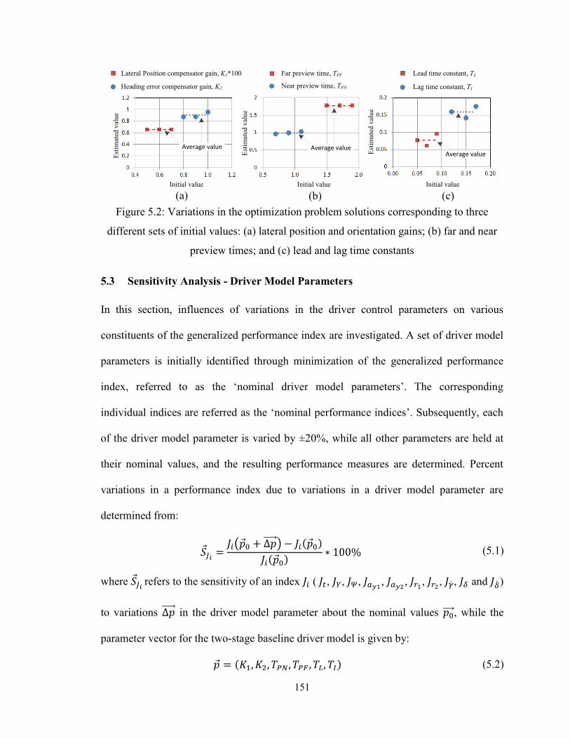
151
Average value Average valueAverage value
Lateral Position compensator gain, K1*100
Heading error compensator gain, K2
Initial value
Near preview time, TPN
Lead time constant, TL
Lag time constant, TI
Far preview time, TPF
Initial value Initial valueInitial value
Est
imat
ed v
alue
Est
imat
ed v
alue
Est
imat
ed v
alue
Figure 5.2: Variations in the optimization problem solutions corresponding to three
different sets of initial values: (a) lateral position and orientation gains; (b) far and near
preview times; and (c) lead and lag time constants
5.3 Sensitivity Analysis - Driver Model Parameters
In this section, influences of variations in the driver control parameters on various
constituents of the generalized performance index are investigated. A set of driver model
parameters is initially identified through minimization of the generalized performance
index, referred to as the ‘nominal driver model parameters’. The corresponding
individual indices are referred as the ‘nominal performance indices’. Subsequently, each
of the driver model parameter is varied by ±20%, while all other parameters are held at
their nominal values, and the resulting performance measures are determined. Percent
variations in a performance index due to variations in a driver model parameter are
determined from:
( ) ( )
( ) (5.1)
where refers to the sensitivity of an index ( , , , , , , , , and )
to variations in the driver model parameter about the nominal values , while the
parameter vector for the two-stage baseline driver model is given by:
( ) (5.2)
(a) (b) (c)

152
Table 5.1 summarizes the percentage variations in the total and individual
performance indices with respect to their respective nominal values. A negative
percentage value represents decrease and thus improvement in a performance measure
with respect to its nominal value. The percentage variation in a performance measure
could help determine the significance and influence of each driver model parameter on
the coupled driver-vehicle system performance.
The results suggest that variations in each of the driver model parameter yield a higher
value of the total performance index ( ) suggesting the validity of the solution of the
minimization problem. Increasing the lateral position and orientation compensatory gains
( and ) help reduce the corresponding indices, and , by -1.7% and -9.1%,
respectively. Enhanced path tracking performance, however, is achieved at the expense of
greater steering effort of the driver, which can be seen from the substantially higher
positive values of and . Employing more distant path information by increasing the
near and far preview time (TPN and TPF) yields lower performance measures related to
vehicle directional responses, namely, the articulation rate ( ), lateral accelerations (
and ) and yaw rates ( and ) of both the units, while the path and orientation
measures ( and ) tend to be substantially higher. The lower peak values of the motion
states of the tractor and the trailing units suggest smoother steering input by the driver,
which is also evident from lower value of . The rate of steering maneuver, , however,
tends to be substantially higher. Increasing TL and decreasing TI by 20% yield only slight
reductions in by 1.6% and 0.4%, respectively, the performance measures
corresponding to steering effort of the driver ( and ) and motion variables of both
units ( , , , and ), however, increased. These suggest greater steering effort

153
demands of the driver and relatively poor directional performance of the coupled driver-
vehicle system.
Table 5.1: Percentage change of the total performance index and its constituents with
variations in the driver model parameters
Control
parameter
Variation
(%)
Percentage change of the performance measures (%)
K1 -20 0.2 2.5 3.5 -2.8 -2.7 -3.1 -2.7 -4.5 -4.3 -17.7
+20 0.3 -1.7 -1.1 2.4 2.3 3.0 2.3 5.4 4.9 25.7
K2 -20 10.8 28.6 3.7 -7.6 -8.8 -10.3 -8.8 -19.1 -12.5 -17.7
+20 8.2 8.8 -9.1 5.1 6.4 8.4 6.4 19.1 11.2 20.3
TPN -20 1.5 3.4 5.6 -1.8 -1.8 -1.1 -1.8 1.7 0.8 6.4
+20 1.7 6.6 7.8 -5.3 -5.3 -4.9 -5.3 -3.0 -3.5 22.2
TPF -20 30.1 -24.9 -19.0 95.7 99.6 103.7 99.6 127.9 106.9 65.1
+20 16.6 67.2 21.2 -45.9 -46.2 -43.3 -46.2 -32.0 -34.4 62.0
TL -20 0.1 2.3 1.9 -2.6 -2.6 -2.9 -2.6 -4.0 -3.5 -11.7
+20 0.2 -1.6 -0.7 2.0 2.0 2.5 2.0 4.3 3.7 18.2
TI -20 0.1 -0.4 1.0 0.5 0.5 0.5 0.5 0.7 0.6 3.1
+20 0.1 0.8 0.5 -0.9 -0.9 -0.9 -0.9 -0.8 -0.8 -1.2
The results also reveal that variations in the far preview time and orientation error
compensatory gain yield the greatest effect on the performance measures of the coupled
system and steering effort of the driver, while variations in the lead and lag time
constants have the lowest influences on the total performance index . The greater
dependency of the estimated values of the TL and TI on their initial values, shown in
Figure 5.2, is thus attributed to relatively lower influences of these two parameters on .
The lead and lag time constants, however, have greater effects on the path tracking
performance ( and ) and steering effort of the driver ( and ) and thus cannot be
excluded in formulation of the driver model (Table 5.1).

154
5.4 Sensitivity Analysis - Variations in Speed and Vehicle Design Parameters
The directional dynamic behavior of the vehicle is generally dependent on a number of
design parameters and forward speed of the vehicle [135,159]. A sensitivity analysis of
the selected motion states of the vehicle is thus undertaken with respect to variations in
the vehicle design parameters and the driving speed. For this purpose, the forward speed,
mass, wheelbase and tandem axle spread of both the units are increased by 20 percent
with respect the nominal values, while the other parameters were held at their respective
nominal values. Due to nearly linear variations in peak directional responses of the
vehicle in the vicinity of the nominal design parameters, the sensitivity analyses in this
section are limited to 20% increase in the vehicle parameters alone. Variations in the
vehicle directional responses are evaluated in terms of (i) peak lateral accelerations of
both units, and ; (ii) peak yaw velocities of both units, and ; and (iii) peak
articulation rate, . Table 5.2 summarizes the variations in the vehicle design and
operating parameters considered in the sensitivity analysis.
It is suggested that variations in the wheelbase and mass of the tractor and the trailing
units affect the yaw moment of inertia of the respective units [148]. Two empirical
relations proposed by Ervin and Guy [148] are used to determine the yaw moment of
inertia of the tractor and the semi-trailer units ( and ) with different wheelbases.
The formulations are based on the load distributions of both the units, given by:
((
) (
) (
)
)
(5.3)
(
)
(5.4)

155
where is the longitudinal distance from axle k (k=1,2 and 3) to the center of gravity of
the tractor, Fzk is normal load on kth
axle (k=1,2,3,4,5) of the articulated vehicle
combination and L2 represents wheelbase of the semi-trailer. In the above formulation,
the subscripts “0” refer to nominal values of the yaw moment of inertia, wheelbase and
normal axle loads of the semi-trailer unit, respectively.
It should be noted that considering fixed distribution of the weights on different axles,
variations in the wheelbases of both the units do not affect the cg position of the
respective unit. Equations (5.3) and (5.4) further suggest that variations in the geometric
parameters yield greater influences on yaw moment of inertia compared to variations in
the inertial parameters. In this study variations in yaw moment of inertia of both the units
are thus assumed to vary only due to considered changes in the geometric parameters.
Table 5.2: Range of vehicle parameters and the nominal values employed in sensitivity
analysis
Nominal value Parameter values
Forward speed, vx (km/h) 100 100
120
Mass of the tractor, m1 (kg) 7269.6 7269.6
8723.5
Mass of the semi-trailer, m2 (kg) 18416 18416
22099.2
Wheelbase of the tractor, L1 (m) 3.6 3.6
4.3
Wheelbase of the semi-trailer, L2 (m) 10.4 10.4
12.5
Tandem axle spread of the tractor, t1 (m) 1.3 1.27
1.52
Tandem axle spread of the semi-trailer, t2 (m) 1.3 1.27
1.52
Considering the yaw-plane articulated vehicle model, described in Appendix A, as a
time-invariant system, the response vector of the vehicle can be expressed as:
156
( ) (5.5)
where ( ) is the state vector and ( ) is the r-dimension
vector of the vehicle design parameters and the forward speed. The influences of
parameters variations on steering characteristics of the vehicle are investigated by
considering:
(5.6)
where is the variation about the nominal vector , while the parameter vector for the
articulated vehicle model is given by:
( ) (5.7)
The sensitivity of the peak response ( ) of the open-loop articulated vehicle to
variations in vehicle parameters is described by the percentage change in a peak response,
( ), with respect to its nominal value, ( ):
( ) ( )
( ) (5.8)
Figure 5.3 illustrates the coordinates of the tractor cg during a step-steer input ( =
1.0 deg) at a speed of 100 km/h subject to 20% increase in each of the vehicle design
parameter, as listed in Table 5.2. The results suggest considerable variations in the
steering characteristics of the vehicle. The results suggest that steering characteristics of
the vehicle tend to vary from understeer to oversteer with increase in the semi-trailer
mass. Increase in the tractor’s mass and wheelbase, on other hand, increase the understeer
tendency of the vehicle. Variations in wheelbase of the trailing unit and tandem axle
spreads of both units, however, yield negligible changes in steering characteristics of the
vehicle.

157
Figure 5.3: Path coordinates of the tractor cg during an open-loop step-steer maneuver at
100 km/h with 20% increase in selected geometric and inertial parameters
Table 5.3 summarizes the results from the sensitivity analysis of the vehicle model
subject to 20 percent increase in selected vehicle design parameters. The percentage
variations in the peak directional responses of the articulated vehicle are evaluated using
Eq. (5.8). A positive and negative percentage value, respectively, represents an increase
and decrease in the peak motion state with respect to that obtained for the nominal
vehicle design parameters.
The results suggest that the peak directional responses of an articulated vehicle are
primarily affected by variations in the forward speed and mass of the trailing unit, while
increase in the wheelbase and tandem axle spread of the semi-trailer have the lowest
effect. Increasing in mass, wheelbase and the tandem axle spread of the tractor unit
resulted in decrease in all the peak directional responses of vehicle. This can be attributed
to increasing understeer tendency of the vehicle. A 20 percent increase in the mass and
tandem axle spread of the semi-trailer unit yields an increase in all the selected responses
of the vehicle, although the influences of tandem axles spread are relatively small
Nominal vehicle parameters
of the
Increase in
oversteer
tendency
Increase in
understeer
tendency

158
compared to that of the semi-trailer mass. Further, an increase in the semi-trailer
wheelbase yields slight reduction in lateral accelerations and yaw rates of both the tractor
and semi-trailer units, while it increases the articulation rate of the vehicle. This suggests
that an increase in the semi-trailer wheelbase may slightly improve the roll stability of the
vehicle, the jackknife potential may increase with a longer trailing unit.
Table 5.3: Percent changes in peak directional responses of the articulated vehicle with
20% increase in the selected parameters
Percentage change of the peak directional responses (%)
Forward speed, vx1 61.1 39.8 67.1 39.1 25.5
Tractor mass, m1 -18.2 -17.5 -18.0 -18.0 -9.9
Tractor wheelbase, L1 -14.7 -14.7 -14.7 -14.7 -12.6
Tractor tandem axle spread, t1 -5.5 -5.4 -5.5 -5.5 -4.5
Semi-trailer mass, m2 32.5 33.0 33.1 33.0 16.1
Semi-trailer wheelbase, L2 -0.2 -0.3 -0.2 -0.2 1.9
Semi-trailer tandem axle spread, t2 0.4 0.4 0.4 0.4 0.1
5.5 Identification of Control Limits of the Driver
The identified driver model parameters and the peak directional response quantities of the
coupled driver-articulated vehicle system are evaluated considering variations in the
selected geometric and inertial parameters, and the forward speed. The model parameters
and peak response measures are compared with those obtained using the nominal vehicle
design parameters under the same maneuver and forward speed. The directional
responses of the coupled driver-articulated vehicle model are further studied to determine
a set of vehicle parameters that could improve the directional performance measures of
the coupled driver-vehicle system.

159
The selected design parameters of the vehicle are permitted to vary within ranges
specified in the weights and dimensional regulations. These regulations include
geometric specifications and axles load limits of different combination vehicles
[160,161]. Owing to variations in the provincial and territorial weights and dimensions
regulations in Canada, a set of standards for the weight and dimension limits of trucks,
which is generally referred as the ‘Memorandum of Understanding (MOU)’, is used to
define the limiting values of geometric and inertial parameters [160].
The simulations are performed assuming a constant perception time ( ) selected as
0.1 s [5,144], while the processing time delay ( ) of the human’s central nervous system
is determined from the regression model formulated in section 3.5.2, as a function of the
vehicle forward speed. The driver’s hand-arm parameters are taken as those reported in
[67]. The peak steer angle and peak steer rate in the generalized performance index, Eq.
(4.22), are limited to those reported by Breuer [132] on the basis of the measured data
( =6.2 deg and =24.8 deg/s) considering the steering ratio equal to 30 for the
articulated vehicle, as described in section 4.5.
5.5.1 Variations in the Forward Speed
The performance characteristics of the coupled driver-vehicle system are investigated
under a double lane-change steering maneuver at four different forward speeds (50, 80,
100 and 120 km/h). Figure 5.4 illustrates the driver model parameters obtained for these
speeds, while the time histories of the front wheels steer angle, , and the tractor cg
coordinates are shown in Figure 5.5. In Figure 5.5, the centerline of the desired roadway
is shown by the thin solid line.

160
The results suggest that vehicle operation at higher forward speeds involves only
slightly higher orientation error compensatory gain K2, but a substantially lower lateral
position compensatory gain, K1. This suggests that the driver is required to undertake
lower compensation to minimize the lateral position error and relatively higher
compensation of the orientation error at higher speeds. Increasing the forward speed also
implies slightly higher compensatory lead time constant of the human driver but
considerably lower lag time constant. This suggests that the driver is required to respond
faster and employ a higher level of prediction at higher speeds. Such trends in driver
control characteristics have also been reported for single unit vehicles [9].
The results also suggested that considering the known ranges of the driver control
limits (Table1.7), the coupled driver-vehicle system would not be able to track the
desired roadway. The minimization problem failed to converge for the maneuver at 120
km/h. The limit constraints on the driver control parameters were thus relaxed in a
sequential manner and the minimization problem was solved. The solutions revealed that
slight relaxation in the lower limit of the lag time constant (TI) could help realize the path
tracking performance in a stable manner. The results thus suggest that the human driver is
required to employ a lower lag time constant (TI) to perform the desired steering
maneuver at the higher speed of 120 km/h, when compared to the maneuvers at lower
speeds. This lag time constant, however, is beyond the reported limits for the human
driver, and suggests that the driver may not be able to perform the double lane-change
maneuver at 120 km/h with acceptable path tracking performance.
The results also suggest that the near and far preview times, TPN and TPF, decrease
with increase in the driving speed, although the resulting near and far preview distances,

161
DPN and DPF, generally increase with the speed. The near preview distance, however,
formed an exception at 120 km/h; it was lower than that obtained at 100 km/h. This can
be attributed to higher TL and considerably lower TI at this speed. The results also show
that increasing the speed invariably yields greater path deviation and relatively lower
peak steer angle (Figure 5.5), which is mostly attributed to employing the lateral
accelerations perception of the human driver within the generalized performance index.
At the higher driving speeds, the proposed driver model, thus, deviates considerably from
the centerline of the desired roadway to minimize the lateral accelerations and yaw
velocities of both the units.
Figure 5.4: Influence of variations in the forward speed on the driver control parameters
during a double lane-change maneuver (50, 80, 100 and 120 km/h)
Figure 5.5: Influence of variations in the forward speed on: (a) path tracking response;
and (b) steer angle of the tractor unit during double lane-change maneuvers
0 50 100 150-1
0
1
2
3
4
Longitudinal coordinate (m)
La
tera
l co
ord
ina
te (
m)
0 50 100 150-3
-2
-1
0
1
2
Longitudinal coordinate (m)
F (
de
g)
Centerline 50 km/h 80 km/h 100 km/h 120 km/h
Lower limit for lag
time constant (0.02 s)
TI = 0.015 s
(a) (b)

162
Table 5.4 summarizes variations in the path tracking measures that can be described by:
(i) peak lateral deviation between the desired path and tractor cg, ; (ii) peak path
deviation in the median segment, ; and (iii) peak heading error, (Figure 5.6). The
peak directional responses of the coupled driver-articulated vehicle system are also
summarized in Table 5.5. The grey shaded areas in the tables indicate the peak directional
responses in terms of path deviation and lateral accelerations of both the units beyond the
selected threshold levels, presented in section 4.5.
0 50 100 150 200-1
0
1
2
3
4
Longitudinal coordinate (m)
La
tera
l co
ord
ina
te (
m)
Ψe
Median segment
Exit segmentYe
Centerline of
the roadYem
Figure 5.6: Path deviation and orientation error of the articulated vehicle
The peak errors in path tracking measures of the driver-vehicle system, as shown in
Table 5.4, suggest that the vehicle driver can successfully perform the selected double
lane-change maneuver for the given vehicle only at 50 and 80 km/h. The driver, however,
exhibits limited control performance at the higher speeds of 100 and 120 km/h. At these
speeds, the peak path deviation of the tractor cg during the median segment, , is
greater than the maximum permissible path deviation (0.5 m, as described in section 4.5).
At 100 and 120 km/h, the peak lateral acceleration of the trailing unit also approaches the
permissible limit of 0.3g, as described in section 4.5. The control of the vehicle at these
speeds would necessitate greater compensation by the driver beyond the known ranges of

163
the driver control limits listed in Table 1.7. The driver would thus be expected to reduce
the speed to execute such a maneuver or relax the path tracking error requirements [14].
Further, the results suggest that the peak articulation rate, peak lateral accelerations
and peak yaw rates of both the tractor and the semi-trailer units increase with increase in
the forward speed. The similar trends were also observed in the open-loop step-steer
responses, presented in section 5.3.2. The results also imply that the peak steer rate
increases with speed, while the peak steer angle decreases with increase in the forward
speed. This suggests that the human driver is required to perform faster steering actions at
the higher driving speeds. It should be also noted that the nominal tractor unit is
understeer (Kus = 0.003) and the semi-trailer unit is oversteer (Kus,t = -0.007). In this case,
the articulation angle of the vehicle remains finite for all the driving speeds considered
[124].
Table 5.4: Influence of variations in the forward speed of the vehicle on peak errors in
path tracking measures tracking responses of the driver-vehicle system
Forward speed
(km/h)
Peak errors in path tracking measures
(m)
(m)
(deg)
50 0.08 0.81 7.39
80 0.27 1.07 7.93
100 0.54 1.22 8.67
120 0.80 1.44 9.71
Table 5.5: Influence of variations in the forward speed of the vehicle on peak directional
responses of the driver-vehicle system
Forward speed (km/h)
Peak directional responses
(m/s2)
(deg/s)
(m/s2)
(deg/s)
(deg/s)
(deg)
(deg/s)
50 1.50 6.16 1.26 5.20 4.70 60.40 115.38
80 2.86 8.10 2.70 6.98 4.85 52.44 138.57
100 3.39 8.85 3.71 7.65 4.87 46.96 142.71
120 3.88 9.80 5.12 8.80 5.36 42.52 269.55

164
5.5.2 Variations in Tractor Design Parameters
The influences of variations in the tractor design parameters on the driver control
demands and directional responses are further evaluated. These include the variations in
the wheelbase ( ), mass ( ) and tandem axle spread ( ) of the tractor unit. The
simulation results may help in identifying the parameters of a driver-adaptive design of a
vehicle.
Tractor Mass
The nominal value of the tractor mass ( =7270 kg) is increased by 29 percent to 9376
kg, so that the load on the tractor steering axle reaches the maximum allowable load of
5500 kg [160]. The nominal value of the tractor mass is then decreased by 29 percent to
obtain the lower value of 5162 kg. Figure 5.7 shows the driver model parameters
obtained for three different tractor masses, while the time-histories of the front wheels
steer angle ( ) and path coordinates of the tractor cg are shown in Figure 5.8.
The results show that a tractor unit with larger weight imposes relatively lower
position compensatory action from the driver to maintain the central lane position (K1),
while a greater steering action is required to minimize the orientation error of the vehicle.
Increasing the tractor mass also implies relatively lower near and far preview times
TPN and TPF, suggesting longer near and far preview distances of the driver. The tractor’s
understeer coefficient tends to increase with increase in the tractor mass, when the
articulation load is held constant, as seen in Figure 5.3. The results thus suggest that a
driver with a longer preview distance would be more suited for control of the vehicle
with relatively oversteer tractor. Such a trend has also been reported for articulated
vehicles [16]. The results also show greater lead (TL) and lower lag time constants (TI) of

165
the vehicle driver, when driving a tractor with larger weight. This suggests that an
articulated vehicle with heavier tractor requires a higher level of prediction and faster
steering responses of the driver to effectively track the desired path.
Figure 5.7: Influence of variations in the tractor mass on the driver control parameters
during a double lane-change maneuver (speed=100 km/h)
Figure 5.8: Influence of variations in the tractor mass on: (a) path tracking response; and
(b) steer angle during a double lane-change maneuver (speed=100 km/h)
Tables 5.6 and 5.7 summarize the peak errors in path tracking measures and peak
directional responses of the driver-articulated vehicle system, respectively. The grey
shaded areas in the tables indicate the identified values that are beyond the selected
threshold levels in terms of lateral deviation and lateral accelerations of both the units,
presented in section 4.5. Considering the acceptable peak lateral deviation, = 0.5 m,
the results suggest that the vehicle driver can successfully perform the given steering
maneuver only with the lowest tractor mass ( =5162.5 kg). The results also suggest that
0 50 100 150-1
0
1
2
3
4
Longitudinal coordinate (m)
La
tera
l co
ord
ina
te (
m)
0 50 100 150-3
-2
-1
0
1
2
Longitudinal coordinate (m)
F (
de
g)
Centerline Tractor mass (5162 kg) Tractor mass (7270 kg) Tractor mass (9376 kg)
(a) (b)

166
increasing the tractor mass increases the path deviation and orientation error of the
vehicle with respect to the desired path (Table 5.6). Further, the peak steer angle
increases with increase in the tractor mass, while the peak steer rate remains nearly
constant, as indicated in Table 5.7. This suggests greater steering effort of the driver
when driving a vehicle with a heavier tractor. The results also reveal decrease in the peak
articulation rate, peak lateral accelerations and peak yaw rates of both the tractor and the
semi-trailer units with increase in the tractor mass. The similar trends were also observed
from the open-loop step-steer response of the vehicle (section 5.3.2).
Table 5.6: Influence of variations in the tractor mass on peak errors in path tracking
measures of the driver-vehicle system (speed=100 km/h)
Tractor mass
(kg)
Peak errors in path tracking measures
(m)
(m)
(deg)
5162.5 0.48 1.13 8.28
7269.6 0.54 1.22 8.67
9375.7 0.58 1.31 9.09
Table 5.7: Influence of variations in tractor mass on peak directional responses of the
driver-vehicle system (speed=100 km/h)
Tractor mass
(kg)
Peak directional responses
(m/s2)
(deg/s)
(m/s2)
(deg/s)
(deg/s)
(deg)
(deg/s)
5162.5 3.43 8.98 3.79 7.81 5.26 41.69 141.18
7269.6 3.39 8.85 3.71 7.65 4.87 46.96 142.71
9375.7 3.35 8.56 3.61 7.44 4.59 53.72 142.92
Tractor Wheelbase
The various weight and dimensions regulations limit the tractor wheelbase ( ) in the 3 to
6.25 m range [160]. The nominal value of the wheelbase of the tractor unit ( =3.6 m) is
thus decreased by 17 percent to the minimum allowable value of 3.0 m. This value is also
increased by 17 percent to obtain the longer value of the tractor wheelbase of 4.2 m. It

167
should be noted that the steering characteristics of the tractor unit tend to vary from
understeer to oversteer, if the vehicle cg is permitted to move toward the rear tandem
axle. This would increase the possibility of a directional instability of the trailing unit,
e.g., jackknifing, if the driving speed approaches the critical value of the tractor.
Figure 5.9 illustrates influence of variations in the tractor wheelbase on the driver
model parameters, which are identified through minimization of the performance index
under the double lane change maneuver at 100 km/h. The results show trends similar to
those observed with increasing the tractor mass. The results suggest that increasing of the
tractor wheelbase yields slightly lower lateral position compensatory gains (K1) but
slightly higher orientation error compensatory gain (K2). This suggests that a tractor unit
with lower wheelbase will impose a slightly higher lateral position compensation demand
on the driver to minimize lateral position error. Increasing the tractor wheelbase also
implies slightly lower near preview time, while the far preview time remains nearly
constant. This suggests that a slightly lesser near preview distance is required for longer
tractor units. The lead time constant, however, increases considerably, while the lag time
constant decreases with increasing tractor wheelbase. The driver is thus required to
respond faster and employ a higher level of prediction, when driving a vehicle with
longer tractor. Figure 5.10 shows time-histories of the front wheels steer angle and
coordinates of the tractor cg obtained for three different values of the tractor wheelbase.
The results show that the vehicle driver tracks nearly the same trajectory, while applying
slightly lower steering effort with a shorter wheelbase tractor unit.

168
Figure 5.9: Influence of variations in the tractor wheelbase on the driver control
parameters during a double lane-change maneuver (speed=100 km/h)
Figure 5.10: Influence of variations in the tractor wheelbase on: (a) path tracking
response; and (b) steer angle during a double lane-change maneuver (speed=100 km/h)
Tables 5.8 and 5.9 summarize the influence of variations in the tractor wheelbase on the
peak errors in path tracking measures and peak directional responses of the driver-
articulated vehicle system, respectively. In the tables, the grey shaded areas indicate the
identified values that are beyond the selected threshold levels in terms of lateral deviation
and lateral accelerations of both the units, presented in section 4.5. The results suggest
that the peak path deviations, and , and peak orientation error of the tractor
unit increases slightly with increase in the tractor wheelbase (Table 5.8). The peak
articulation rate, peak lateral accelerations and peak yaw rates of both the units, however,
decrease with increase in the wheelbase (Table 5.9). The similar trends were also
0 50 100 1500
1
2
3
4
Longitudinal coordinate (m)
La
tera
l co
ord
ina
te (
m)
0 50 100 150-3
-2
-1
0
1
2
Longitudinal coordinate (m)
F (
de
g)
Centerline Tractor wheelbase (3.0 m) Tractor wheelbase (3.6 m) Tractor wheelbase (4.21 m)
(a) (b)

169
observed from the open-loop step steer maneuver responses (section 5.3.2). The
reductions in the directional responses of the vehicle are mostly attributed to increase in
the tractor yaw moment of inertia and understeer coefficient of the vehicle with increase
in the tractor wheelbase. The results also show that the peak steer angle and peak steer
rate increase with increase in the tractor wheelbase, suggesting greater steering effort
from the driver when driving a vehicle with relatively more understeer tractor.
Table 5.8: Influence of variations in tractor wheelbase on peak errors in path tracking
measures of the driver-vehicle system (speed=100 km/h)
Tractor
wheelbase
(m)
Peak errors in path tracking measures
(m)
(m)
(deg)
3.00 0.51 1.14 8.55
5.61 0.54 1.22 8.67
4.21 0.55 1.26 8.72
Table 5.9: Influence of variations in tractor wheelbase on peak directional responses of
the driver-vehicle system (speed=100 km/h)
Tractor wheelbase
(m)
Peak directional responses
(m/s2)
(deg/s)
(m/s2)
(deg/s)
(deg/s)
(deg)
(deg/s)
3.00 3.53 9.22 3.83 7.90 4.96 44.07 139.87
5.61 3.39 8.85 3.71 7.65 4.87 46.96 142.71
4.21 3.34 8.67 3.64 7.50 4.70 51.09 147.64
Tractor Tandem Spread
The weights and dimensions regulations permit the tractor tandem axle spread ( ) in the
1.2 to 1.85 m range [160]. The nominal value of tandem axle spread of the tractor unit
( =1.3 m) is thus increased by 42 percent to attain the maximum permissible value of
1.85 m. The sensitivity analysis also considered an alternate spread of 1.6. Figure 5.11
summarizes the influence of variations in the axle spread on the driver control
parameters. Figure 5.12 shows the time-histories of the corresponding front wheels steer

170
angle ( ) and path coordinates of the tractor cg. The results suggest only minimal effect
of axle spread on the control demands of the driver, except for the lead time constant, TL,
which tends to be lower with higher tandem spread. This suggests some relaxation on the
predictive steering control action of the driver when the tractor tandem axle spread is
increased. The results also show nearly negligible effect on the front wheels steer angle
and the path tracking response.
Figure 5.11: Influence of variations in the tractor axle spreads on the driver control
parameters during a double lane-change maneuver (speed=100 km/h)
Figure 5.12: Influence of variations in the tractor axle spreads on: (a) path tracking
response; and (b) steer angle during a double lane-change maneuver (speed=100 km/h)
Tables 5.10 and 5.11 summarize the influence of variations in the tractor tandem axle
spread on the peak errors in path tracking measures and peak directional responses of the
driver-articulated vehicle system. The grey shaded areas indicate that the response
0 50 100 150-1
0
1
2
3
4
Longitudinal coordinate (m)
La
tera
l co
ord
ina
te (
m)
0 50 100 150-3
-2
-1
0
1
2
Longitudinal coordinate (m)
F (
de
g)
Centerline Axle spread (1.3 m) Axle spread (1.6 m) Axle spread (1.85 m)
(a) (b)

171
measures in terms of , and exceed the threshold levels, presented in section
4.5. The results suggest that the peak path lateral deviations, and , and orientation
error of the vehicle increase only slightly with increase in the tractor tandem axle spread
(Table 5.10), which is mostly attributed to lower lead time constant of the driver. The
results also show that the peak steer angle and peak steer rate increase slightly with
increase in the tractor tandem axle spread, suggesting greater steering effort demand on
the driver. The peak articulation rate, peak lateral accelerations and peak yaw rates of
both the units decrease slightly with increase in the tandem axle spread (Table 5.11), as
observed for the open-loop step-steer responses. The minimal effect of tandem axle
spread on the driver control parameters and thus the directional responses of the vehicle
can be attributed to its minimal effect on the steering characteristics and understeer
coefficient of the tractor.
Table 5.10: Influence of variations in tractor axle spreads on peak errors in path tracking
measures of the driver-vehicle system (speed=100 km/h)
Tractor tandem
axle spread
(m)
Peak errors in path tracking measures
(m)
(m)
(deg)
1.3 0.54 1.22 8.67
1.6 0.56 1.25 8.79
1.85 0.58 1.27 8.85
Table 5.11: Influence of variations in tractor axle spreads on peak directional responses
of the driver-vehicle system (speed=100 km/h)
Tractor tandem
axle spread
(m)
Peak directional responses
(m/s2)
(deg/s)
(m/s2)
(deg/s)
(deg/s)
(deg)
(deg/s)
1.3 3.39 8.85 3.71 7.65 4.87 46.96 142.71
1.6 3.34 8.68 3.64 7.50 4.55 48.89 148.38
1.85 3.30 8.56 3.58 7.39 4.27 50.71 154.06

172
5.5.3 Variations in Semi-Trailer Design Parameters
Influence of variations in selected semi-trailer design parameters on the driver control
and directional responses of the coupled driver-vehicle system are investigated in the
similar manner. The design parameters include the semi-trailer mass ( ), wheelbase
( ) and tandem axle spread ( ).
Semi-Trailer Mass
The semi-trailer mass ( ) includes the mass of the trailing unit with the payload and
mass of the rear tandem axles. The nominal value of the semi-trailer mass (26018 kg) is
increased by 14 percent, so that the load on the tandem axle of the trailing unit
approaches the maximum allowable axle load of 17000 kg [160]. The semi-trailer mass is
also decreased by 14 percent to achieve the semi-trailer mass of 22434 kg. A ‘0 kg’
payload condition is also considered to examine the driver control demands and
responses of an unloaded vehicle. The semi-trailer mass in this condition is taken as 7602
kg, which includes the mass of the trailing unit and that of rear tandem axles. It should be
noted that a higher payload can lead to a greater oversteer tendency of the semi-trailer
unit, which may result in lower roll and yaw stability limits of the vehicle combination.
Figures 5.13 and 5.14, respectively, illustrate the influences of variations in the semi-
trailer mass on the driver control parameters, and time-histories of the front wheels steer
angle ( ) and the path coordinates of the tractor cg. The results suggest that increasing
the semi-trailer mass can lead to lower lateral position and orientation compensatory
gains. This is likely due to lower understeer coefficient of the trailer with greater mass or
payload. Increasing the semi-trailer mass, however, would require greater near and far
preview times, TPN and TPF, and thus the respective distances. The driver would thus be

173
required to employ longer preview distances. Furthermore, a heavier trailer would impose
a higher level of path prediction by the driver, as it is seen from the increasing lead time
constant (TL). The lag time constant of the driver (TI), however, decreases with increase
in the trailer mass. The results thus suggest that driving a vehicle combination with
higher payload would require the driver to employ longer preview distances, faster
reaction and higher level of path prediction. The steering and path tracking responses of
the driver show that increasing the payload tends to reduce the peak steer angle, while the
effect on path tracking performance is minimal, as shown in Figure 5.14.
Figure 5.13: Influence of variations in the semi-trailer mass on the driver control
parameters during a double lane-change maneuver (speed=100 km/h)
Figure 5.14: Influence of variations in the semi-trailer mass on: (a) path tracking
response; and (b) steer angle during a double lane-change maneuver (speed=100 km/h)
Tables 5.12 and 5.13 summarize variations in the peak errors in path tracking
measures and peak directional responses of the coupled driver-articulated vehicle system,
0 50 100 150-1
0
1
2
3
4
Longitudinal coordinate (m)
La
tera
l co
ord
ina
te (
m)
0 50 100 150-3
-2
-1
0
1
2
Longitudinal coordinate (m)
F (
de
g)
Centerline Trailer mass (7602 kg) Trailer mass (22434 kg) Trailer mass (26018 kg) Trailer mass (29602 kg)
(a) (b)

174
respectively. The grey shaded areas indicate that the response measures in terms of ,
and exceed the threshold levels, presented in section 4.5. The results suggest that
increasing the semi-trailer mass increases the path deviation and orientation error of the
vehicle with respect to the desired path (Table 5.12). The results also show that the peak
steer angle and peak steer rate of the driver decrease with increase in the semi-trailer
mass. This suggests that the driver tends to relax on the path deviation in order to limit
the magnitudes of lateral acceleration and yaw rate of the trailing unit. This is also
evident from the relatively lower compensation gains (K1 and K2), and steer angle and
steer rate of the heavier semi-trailer. Increase in the semi-trailer mass also yields higher
magnitudes of and . The corresponding tractor yaw rate also increases only
slightly. The relatively lower steer angle and rate also results in lower tractor lateral
acceleration and articulation rate of the combination.
Table 5.12: Influence of variations in semi-trailer mass on peak errors in path tracking
measures of the driver-vehicle system (speed=100 km/h)
Semi-trailer
mass (kg)
Peak errors in path tracking measures
(m)
(m)
(deg)
7602 0.45 1.20 8.58
22434 0.53 1.22 8.68
26018 0.54 1.22 8.67
29602 0.57 1.26 8.78
Table 5.13: Influence of variations in semi-trailer mass on peak directional responses of
the driver-vehicle system (speed=100 km/h)
Semi-trailer
mass (kg)
Peak directional responses
(m/s2)
(deg/s)
(m/s2)
(deg/s)
(deg/s)
(deg)
(deg/s)
7602 3.93 8.62 3.28 6.77 4.92 73.96 213.76
22434 3.45 8.65 3.56 7.34 4.89 51.51 165.73
26018 3.39 8.85 3.71 7.65 4.87 46.96 142.71
29602 3.26 8.95 3.81 7.86 4.58 42.01 135.73
175
Semi-Trailer Wheelbase
The various weight and dimensions regulations limit the semi-trailer wheelbase ( ) in
the 6.25 to 12.5 m range [160]. The nominal wheelbase of the trailer unit ( =10.4 m) is
thus increased by 20 percent to the maximum allowable value of 12.5 m. This value is
also decreased by 20 percent to obtain a lower value of the trailer wheelbase of 8.3 m.
Figure 5.15 illustrates influence of variations in the semi-trailer wheelbase on the driver
control parameters, identified through minimization of the performance index under the
double lane change maneuver performed at 100 km/h. The time-histories of the front
wheels steering angle and the coordinates of the tractor cg obtained for three different
values of the semi-trailer wheelbase are illustrated in Figure 5.16.
The results show that increasing the semi-trailer wheelbase yields lower lateral
position compensatory gain (K1), while orientation error compensatory gain (K2) remains
almost constant. This suggests a lower lateral position compensation demand on driver
when driving a vehicle with longer semi-trailer wheelbase. Increasing the semi-trailer
wheelbase also implies greater near and far preview times, TPN and TPF, suggesting that
more distant near and far target points are required. Further, the compensatory lead time
constant (TL) increases considerably, while the lag time constant (TI) decreases slightly
with increasing semi-trailer wheelbase. It is thus concluded that a shorter trailing unit can
be best adapted to a driver with lower prediction skill, slower reaction time and shorter
preview distances. Yang et al. [16] also observed a similar trend in a study of driver-
adaptive commercial vehicle designs. The results show that the vehicle driver tracks
nearly the same trajectory, irrespective of the trailer wheelbase, although a slightly higher
steering angle is applied for a longer wheelbase trailing unit.

176
Figure 5.15: Influence of variations in the semi-trailer wheelbase on the driver control
parameters during a double lane-change maneuver (speed=100 km/h)
Figure 5.16: Influence of variations in the semi-trailer wheelbase on: (a) path tracking
response; and (b) steer angle during a double lane-change maneuver (speed=100 km/h)
Tables 5.14 and 5.15 summarize the influence of variations in the semi-trailer
wheelbase on the peak errors in path tracking measures and peak directional responses of
the driver-articulated vehicle system, respectively. The results reveal that a 20 percent
decrease in the semi-trailer wheelbase yields considerably lower path deviation in the
median segment, in the order of 16%. The peak lateral path deviation and orientation
error, and , of the tractor unit also decreases, although the changes are very small
(Table 5.14). The results also suggest that the peak steer angle increases only slightly
with increase in the semi-trailer wheelbase, while the peak lateral accelerations and yaw
0 50 100 150-1
0
1
2
3
4
Longitudinal coordinate (m)
La
tera
l co
ord
ina
te (
m)
0 50 100 150-3
-2
-1
0
1
2
Longitudinal coordinate (m)
F (
de
g)
Centerline Trailer wheelbase (8.3 m) Trailer wheelbase (10.4 m) Trailer wheelbase (12.5 m)
(a) (b)

177
rates of both the units decrease (Table 5.15). The articulation rate of the vehicle,
however, increases with the semi-trailer wheelbase, which is mostly attributed to increase
in the peak steer rate. The similar trends were also observed from the open-loop step steer
maneuver responses presented in section 5.3.2. The substantial reductions in directional
responses of the vehicle with increase in the trailer wheelbase are mostly due to
considerable increase in the semi-trailer yaw moment of inertia.
Table 5.14: Influence of variations in semi-trailer wheelbase on peak errors in path
tracking measures of the driver-vehicle system (speed=100 km/h)
Semi-trailer
wheelbase
(m)
Peak errors in path tracking measures
(m)
(m)
(deg)
8.3 0.45 1.20 8.65
10.4 0.54 1.22 8.67
12.5 0.57 1.23 8.76
Table 5.15: Influence of variations in semi-trailer wheelbase on peak directional
responses of the driver-vehicle system (speed=100 km/h)
Semi-trailer
wheelbase (kg)
Peak directional responses
(m/s2)
(deg/s)
(m/s2)
(deg/s)
(deg/s)
(deg)
(deg/s)
8.3 3.74 9.53 4.28 8.83 4.10 46.42 130.51
10.4 3.39 8.85 3.71 7.65 4.87 46.96 142.71
12.5 3.15 8.28 3.28 6.76 5.51 47.75 166.67
Semi-Trailer Tandem Spread
The weights and dimensions regulations permit the semi-trailer tandem axle spread ( ) in
the 1.2 to 1.85 m range [160]. The nominal tandem axle spread of the trailer unit ( =1.3
m) is thus increased to attain the maximum permissible value of 1.85 m. The sensitivity
analysis also considered an alternate spread of 1.6 m. Figure 5.17 summarizes the
influence of variations in the semi-trailer tandem axle spread on the driver control
parameters, while Figure 5.18 shows time-histories of the corresponding front wheels

178
steer angle and path coordinates of the tractor cg under the double-lane change
maneuvers at 100 km/h.
The results suggest that increasing the semi-trailer axle spread yields greater lateral
position compensatory gains (K1), while the orientation error compensatory gain (K2)
remains nearly constant. This suggests that a trailing unit with longer axle spread will
impose greater lateral position compensation demand on the driver to minimize the lateral
position error. Variations in the semi-trailer axle spread also yield only minimal effect on
the near as well as far preview times. While the compensatory lead time constant
decreases considerably, the lag time constant increases slightly with increase in the trailer
axle spread. The driver is thus required to respond faster and employ a higher level of
prediction, when driving a vehicle with shorter semi-trailer axle spread. The results also
show nearly negligible effect on the front wheels steer angle and path tracking responses.
Figure 5.17: Influence of variations in the semi-trailer axle spreads on the driver control
parameters during a double lane-change maneuver (speed=100 km/h)

179
Figure 5.18: Influence of variations in the semi-trailer axle spreads on: (a) path tracking
response; and (b) steer angle during a double lane-change maneuver (speed=100 km/h)
Tables 5.16 and 5.17 summarize the influence of variations in the semi-trailer tandem
axle spread on the peak errors in path tracking measures and peak directional responses
of the driver-articulated vehicle system. The results suggest that the peak lateral
deviations, and , and orientation error of the vehicle ( ) decrease with increase in
the semi-trailer tandem axle spread (Table 5.16), which is mostly attributed to greater
lateral position compensation gain (K1). The improved path tracking performance,
however, is achieved at the expense of increase in the peak articulation rate, peak lateral
accelerations and peak yaw rates of both the units. The peak steer angle and peak steer
rate also increase, suggesting greater steering effort demand on the driver with increase in
axle spread of the trailing unit (Table 5.17).
Table 5.16: Influence of variations in semi-trailer axle spread on peak errors in path
tracking measures of the driver-vehicle system (speed=100 km/h)
Semi-trailer
tandem spread
(m)
Peak errors in path tracking measures
(m)
(m)
(deg)
1.3 0.54 1.22 8.67
1.6 0.52 1.20 8.62
1.85 0.49 1.20 8.54
0 50 100 150-1
0
1
2
3
4
Longitudinal coordinate (m)
La
tera
l co
ord
ina
te (
m)
0 50 100 150-3
-2
-1
0
1
2
Longitudinal coordinate (m)
F (
de
g)
Centerline Axle spread (1.3 m) Axle spread (1.6 m) Axle spread (1.85 m)
(a) (b)

180
Table 5.17: Influence of variations in semi-trailer axle spread on peak directional
responses of the driver-vehicle system (speed=100 km/h)
Semi-trailer tandem
spread
(m)
Peak directional responses
(m/s2)
(deg/s)
(m/s2)
(deg/s)
(deg/s)
(deg)
(deg/s)
1.3 3.39 8.85 3.71 7.65 4.87 46.96 142.71
1.6 3.49 9.06 3.79 7.82 5.06 47.88 154.05
1.85 3.61 9.34 3.90 8.04 5.34 49.08 158.99
5.6 Summary
A yaw-plane model of a five-axle articulated vehicle is developed and coupled with a
two-stage preview driver model, referred to as the ‘baseline driver model’, which
involves simultaneous control of lateral position and orientation errors of the vehicle. The
driver’s control limits are investigated considering variations in a number of selected
vehicle design parameters under the standardized double lane-change maneuver
performed at different forward speeds.
The results suggested that at the higher speeds of 100 and 120 km/h, the lateral path
deviation and the lateral accelerations of both the tractor and semi-trailer units are beyond
the defined threshold limits. The results further showed that a light-weight tractor with
shorter wheelbase and shorter tandem axle spread yields improved path tracking
performance of the vehicle and reduced steering effort of the driver. The results also
suggest that the driver can effectively track the desired roadway while driving a shorter
semi-trailer with lower payload. Increasing the tandem axle spread of the semi-trailer unit
can also improve the path tracking performance of the vehicle, while it may result in
greater rate of tire wear. Table 5.17 summarizes the influences of variations in the
forward speed and vehicle design parameters on the peak path deviation, and peak steer
angle and peak steer rate of the driver. The positive and negative signs indicate increase

181
and decrease in a response quantity with increasing of a design or operating variable,
respectively.
It has been suggested that enhancing the driver's perception of vehicle motion
variables may help the driver to improve its path tracking performance. Considering
different motion feedbacks to improve the path tracking and directional responses of the
vehicle will be examined in the subsequent chapter.
Table 5.18: Influences of variations in the forward speed and vehicle design parameters
on path tracking performance and steering response of the driver
Vehicle unit Variable Peak lateral
deviation
Peak steer
angle Peak steer rate
Tractor
Forward speed + - +
Mass + + +
Wheelbase + + +
Axle spread + + +
Semi-trailer
Payload + - -
Wheelbase + + +
Axle spread - + +

182
6 CHAPTER 6
IDENTIFICATION OF EFFECTIVE MOTION CUES PERCEPTION
6.1 Introduction
Under certain driving speeds, a severe vehicle response may occur as the driver tracks the
desired roadway, such as rollover or excessive articulation rate of the articulated vehicle.
The vehicle driver, in general, controls these critical responses of the vehicle by
decreasing the forward speed of the vehicle or by relaxing the path tracking error
requirements. These imply that the human driver control actions depend not only to the
path information, but also on the driver's perception of directional responses of both the
tractor and trailing units. It is thus suggested that considering or enhancing the driver's
perception of vehicle motion variables may help the driver to improve its path tracking
performance while limiting its control demands. This can be examined by involving
different motion states of the vehicle in formulation of the driver model and in evaluating
the driver’s steering effort demands and the path tracking performance of the coupled
driver-vehicle system. For this purpose, the proposed two-stage preview driver model,
referred to as the baseline driver model, is modified by adding the driver's perception of
different vehicle motion cues.
A number of driver model structures are formulated by integrating different
combinations of perceived motion cues to the baseline driver model coupled with the
yaw-plane articulated vehicle model. The relative contributions of additional sensory
feedbacks are investigated through careful examinations of the directional response
quantities and corresponding performance measures in order to identify secondary cues

183
that could facilitate vehicle path tracking. The driver control parameters are identified
through minimization of the generalized performance index, Eq. (4.19), subject to
constraints imposed by the human driver’s compensation limits (Table 1.7). The sensory
feedback cues that help to reduce path deviation and steering effort demands of the driver
can be utilized as additional sensory feedbacks that provide important guidance for
designs of driver-assist systems (DAS).
6.2 Perception of Different Vehicle States by the Human Driver
It is hypothesized that under medium- and low-speed steering maneuvers the driver is
able to track the desired path by considering only the lateral position and orientation
errors of the vehicle relative to its surroundings. These errors can be predicted and
perceived through the driver’s path prediction process and visual sensory cues,
respectively [7,8,10]. At higher speeds, the human drivers, however, exhibit limited
control performance that generally impose greater demands on the drivers’ decisions and
control abilities. It is suggested that in these situations, a qualitative perception of
additional vehicle states can help the driver to improve its path tracking performance
[11]. In the case of articulated vehicles, the human driver can perceive the linear
acceleration and rotational velocity of the tractor unit in a qualitative manner through its
vestibular and body-distributed kinesthetic cues [32]. The perception of the various
motion states of the trailing units also assists the human driver to undertake effective
steering control actions. These feedback cues may include articulation rate, lateral
accelerations, yaw velocities, roll angles and roll rates of both the units, which can be
perceived through in-vehicle sensors or from the driver’s experience [9]. Considering
only the lateral dynamics of the articulated vehicle, additional vehicle states in this study

184
are limited to lateral accelerations and yaw rates of the tractor and semi-trailer units ( ,
, and ) and articulation rate ( ).
A total of 10 model structures are formulated by adding different motion cues
corresponding to directional responses of both the units of the vehicle to the baseline
model, as illustrated in Table 6.1. The baseline driver model (structure 1) only involves
the driver’s perception of the lateral position and orientation errors that have been
commonly employed in reported driver models. Nine combinations of motion cues
perception, which are described by structures 2 to 10, describe the driver’s perception of
different motion cues in a sequential manner.
Table 6.1: The proposed driver model structures employing driver’s perceptions of
different motion cues
Structure
Path information Perceived feedback variables
Tractor unit Semi-trailer unit
Lateral
position
error
Heading
error lateral
acceleration
yaw
rate
lateral
acceleration
yaw
rate
articulation
rate
Structure 1
Structure 2
Structure 3
Structure 4
Structure 5
Structure 6
Structure 7
Structure 8
Structure 9
Structure 10
The human perception of instantaneous vehicle states is invariably described
considering two essential characteristics: (i) perception delay time [5]; and (ii) perception
threshold value [32], as described in section 1.2.1. The simulations are performed

185
assuming a constant perception delay time, selected as 0.1 s. The minimum perceivable
linear accelerations and yaw rates of both the units, which can be perceived either by the
driver’s body-distributed sensors or via in-vehicle sensors, are set as 0.06 m/s2
and 0.7
deg/s, respectively [5,32].
6.3 Identification of Effective Motion Cues Perception
Relative significance of additional sensory feedbacks related to the path tracking
performance and directional dynamic measures of the vehicle is examined by adding
different motion cues to the baseline driver model structure (structure 1). These feedback
variables, which are related to the selected tractor and semi-trailer motions cues, are
integrated in the decision making function, ( ), described in Eq. (4.13). Considering a
clear visibility condition, simulations are performed to determine the vehicle responses
and the individual performance indices while considering nine different combinations of
perceived motion cues (Table 6.1). For this purpose, the driver control parameters for
each structure are identified through minimization of the generalized performance index,
Eq. (4.19), within the practical ranges of control gains that relate to the human driver’s
characteristics, which are summarized in Table 6.2. The peak directional responses and
different performance measures of the vehicle coupled with different driver model
structures are then compared to those obtained using the baseline driver model in order to
evaluate the relative significance of each set of motion perception at different speeds and
various vehicle design parameters. The vehicle design parameters include the variations
in the wheelbases, masses and tandem axle spreads of the tractor and the semi-trailer
units.

186
Table 6.2: Range of human driver’s control parameters
Control variables Unit Range
Near and far preview times, TN and TF s 0.10 - 2.50
Lead time constant, TL s 0.02 – 3.00
Lag time constant, TI s 0.02 - 0.80
Lateral position error compensatory gain, K1 rad/m 1e-5 - 1.40
Orientation error compensatory gain , K2 rad/rad 0.10 - 1.85
Lateral acceleration compensatory gains, K3 and K4 rad.s2/m 0.00 - 1.00
Yaw rate compensatory gains, K5 and K6 rad.s/rad 0.00 - 1.00
Articulation rate compensatory gain, K7 rad.s/rad 0.00 - 1.00
6.3.1 Influence of Additional Feedback Cues - High Speed Driving
During double lane-change maneuvers at the higher speeds of 100 and 120 km/h, the
baseline driver model coupled with the articulated vehicle model suggested that the path
deviation of the tractor cg in the median segment is greater than the permissible threshold
value, 0.5 m (Table 5.4). Further, at 120 km/h the vehicle driver is required to employ a
considerably low lag time constant beyond its limit constraints and the driver failed to
perform the selected maneuver. The results thus suggest that the vehicle driver exhibits
limited control capabilities to perform the selected maneuver at the speeds of 100 and 120
km/h. In such situations, introducing the perception of the vehicle motion variables may
help the driver to improve its path tracking performance and to perform the desired
maneuver in a controlled and stable manner. Contributions of additional feedback cues to
improve the path tracking performance and directional response measures of the coupled
driver-vehicle system are discussed considering nine combinations of vehicle motions
cues that are integrated with the baseline driver model.
Table 6.3 summarizes the influence of integrating different motion variables to the
baseline driver model on the total performance index ( ) together with its various
constituents during double lane-change maneuvers at the speed of 100 km/h. Table 6.4
presents the percent changes in the peak errors of the path tracking measures and peak

187
directional responses of the vehicle relative to those obtained using the baseline model
structure (structure 1) at 100 km/h. A negative and positive value of the percent change
indicates a decrease and increase in the response quantity compared to that of the baseline
model, respectively. The grey shaded areas in the tables indicate the notable variations in
the selected measures when different motion states of the vehicle are involved in
formulation of the driver model.
Table 6.3: Variations in the total performance index and its constituents by considering
different driver model structures considering nominal vehicle parameters at a constant
speed of 100 km/h
Structure Performance index constituents
Structure 1 0.7515 0.0758 0.1906 0.2119 0.0916 0.0779 0.0513 0.0068 0.0028 1.4603
Structure 2 0.7542 0.0780 0.1889 0.2095 0.0904 0.0770 0.0499 0.0067 0.0029 1.4577
Structure 3 0.7520 0.0786 0.1901 0.2100 0.0891 0.0772 0.0454 0.0063 0.0020 1.4509
Structure 4 0.7336 0.0753 0.1960 0.2181 0.0942 0.0802 0.0525 0.0069 0.0027 1.4595
Structure 5 0.7332 0.0763 0.1953 0.2167 0.0931 0.0797 0.0505 0.0068 0.0026 1.4541
Structure 6 0.7065 0.0749 0.2040 0.2271 0.0979 0.0835 0.0544 0.0071 0.0027 1.4582
Structure 7 0.7372 0.0777 0.1942 0.2150 0.0914 0.0790 0.0470 0.0065 0.0019 1.4500
Structure 8 0.7183 0.0772 0.1980 0.2191 0.0933 0.0806 0.0484 0.0066 0.0021 1.4436
Structure 9 0.7192 0.0776 0.1996 0.2210 0.0940 0.0813 0.0487 0.0067 0.0021 1.4502
Structure 10 0.7504 0.0790 0.1902 0.2099 0.0891 0.0772 0.0454 0.0063 0.0022 1.4497
At the constant speed of 100 km/h, involving the lateral acceleration of the tractor unit
( ) alone, as seen in structure 3, and the lateral accelerations of both the units ( and
) together with the articulation rate of the vehicle ( ), structure 10, yield the most
beneficial effects to enhance the performance indices related to , , , , and ,
and corresponding peak directional responses (Tables 6.3 and 6.4). The results further
suggest that the lowest values of the path tracking performance ( and ) and peak path
deviation in the median segment ( ), can be achieved by using the yaw rate ( ) of the
trailing unit alone (structure 6). Including the and also reduce the peak steer rate of

188
the driver, while its effect on peak steer angle is minimal. It can be thus suggested that
combining the trailer yaw rate and lateral accelerations of the tractor and trailing units
may leads to considerable improvement in path tracking and performance indices
corresponding to directional responses of the vehicle. Employing and (structure 8)
and and (structure 9) in addition to the lateral position and orientation errors of the
baseline driver model greatly improve the total performance index of the vehicle ( ),
and considerably reduce the path deviation ( ) of the coupled driver-vehicle system.
Table 6.4: Relative changes in path tracking and directional response measures of the
coupled driver-vehicle system integrating different feedback cues compared to those
obtained from the baseline model (structure 1) considering nominal vehicle parameters at
constant speed of 100 km/h
Structure Percentage variations in the peak path deviations and peak directional responses (%)
(m)
(deg)
(m/s2)
(deg/s)
(m/s2)
(deg/s)
(deg/s)
(deg)
(deg/s)
Structure 2 0.28 -0.01 -0.73 -1.16 -1.27 -1.27 0.25 -1.47 6.83
Structure 3 2.61 -0.89 -3.24 -10.27 -5.98 -5.98 -17.95 -10.52 19.79
Structure 4 -3.41 -0.66 0.76 0.68 0.79 0.79 0.45 0.73 -2.62
Structure 5 -2.13 -0.91 -2.42 -2.05 -1.65 -1.65 -2.30 -1.65 5.56
Structure 6 -7.86 -1.28 3.01 1.84 2.48 2.48 3.38 0.85 -2.16
Structure 7 -1.40 -1.23 -0.57 -8.72 -3.59 -3.59 -14.71 -10.07 9.38
Structure 8 -4.53 -0.72 -2.30 -5.72 -2.55 -2.55 -9.80 -5.87 6.10
Structure 9 -3.41 -1.47 0.19 -8.56 -3.42 -3.42 -12.25 -9.52 12.58
Structure 10 3.44 -0.80 -3.10 -10.36 -6.28 -6.28 -17.80 -10.52 24.01
Table 6.5 summarizes the influence of involving different combinations of feedback
cues on the total performance index ( ) together with its various elements at 120 km/h.
At the same driving speed, Table 6.6 presents the percent changes in the peak errors and
peak directional responses of the vehicle relative to those obtained using the baseline
model structure (structure 1). A negative and positive value of the percent change in the
table indicates a decrease and increase in the response quantity, respectively. The grey

189
shaded areas indicate the significant variations in the selected response quantities
compared to those obtained from the baseline driver model.
The results suggest that including the feedback cues from lateral accelerations and
yaw rates of both the units (structures 7 to 10) improves the total performance index of
the coupled driver-vehicle system (Table 6.5). At the higher speed of 120 km/h,
employing only the lateral position and heading angle errors, as described in structure 1,
yields the lowest performance measure related to the tractor lateral acceleration ( ),
while its peak path deviation ( ) is greater than the maximum permissible value, 0.5 m
(Table 5.4).
Table 6.5: Variations in the total performance index and its constituents by considering
different driver model structures considering nominal vehicle parameters at a constant
speed of 120 km/h
Structure Performance index constituents
Structure 1 0.9391 0.0797 0.2081 0.2750 0.0793 0.0702 0.0541 0.0040 0.0060 1.7155
Structure 2 0.9247 0.0796 0.2114 0.2796 0.0806 0.0714 0.0550 0.0040 0.0055 1.7118
Structure 3 0.8901 0.0785 0.2192 0.2892 0.0831 0.0738 0.0557 0.0041 0.0060 1.6997
Structure 4 0.8828 0.0794 0.2224 0.2954 0.0854 0.0754 0.0592 0.0043 0.0062 1.7106
Structure 5 0.8933 0.0792 0.2180 0.2888 0.0834 0.0737 0.0572 0.0042 0.0061 1.7040
Structure 6 0.8522 0.0756 0.2373 0.3108 0.0881 0.0793 0.0552 0.0039 0.0041 1.7064
Structure 7 0.8406 0.0764 0.2353 0.3060 0.0863 0.0781 0.0521 0.0037 0.0041 1.6826
Structure 8 0.7814 0.0728 0.2584 0.3374 0.0953 0.0861 0.0584 0.0042 0.0044 1.6982
Structure 9 0.7938 0.0737 0.2535 0.3309 0.0931 0.0844 0.0561 0.0039 0.0041 1.6936
Structure 10 0.9324 0.0737 0.2103 0.2677 0.0751 0.0683 0.0428 0.0033 0.0037 1.6773
At a constant speed of 120 km/h, the simulation results show almost similar trends as
those obtained for the different driver model structures at the speed of 100 km/h and
summarized in Tables 6.3 and 6.4. For instance, employing the yaw velocity of the
trailing unit ( ) alone (structure 6) or combinations of the lateral accelerations of both
the units ( or ) and yaw rate of the trailing unit (structures 8 and 9, respectively)

190
yield substantial enhancement in and (Table 6.6) and a good improvement of
corresponding performance measures, and (Table 6.5). These improvements,
however, are achieved at the expense of increasing the peak directional responses of the
vehicle ( , , and ). Further, adding the lateral accelerations of both the units
together with the articulation rate, as seen in structure 10, yields the greatest
improvement in the total performance index ( ) and also improve the performance
indices related to , , , , and , while the contribution of these feedbacks to the
path tracking performance are minimal. At 120 km/h, the peak the articulation rate of the
vehicle can be effectively reduced by adding the feedback cues of and (structure
7), and (structure 8), and , and (structure 10) to the baseline driver
model.
Table 6.6: Relative changes in path tracking and directional response measures of the
coupled driver-vehicle system integrating different feedback cues compared to those
obtained from the baseline model (structure 1) considering nominal vehicle parameters at
a constant speed of 120 km/h
Structure
Percentage variations in the peak path deviations and peak directional responses (%)
(m)
(deg)
(m/s2)
(deg/s)
(m/s2)
(deg/s)
(deg/s)
(deg)
(deg/s)
Structure 2 -1.94 -0.35 0.55 1.00 0.98 0.98 0.29 1.85 0.66
Structure 3 -0.01 -0.87 3.76 0.55 1.39 1.39 0.49 4.44 3.69
Structure 4 -4.12 -1.24 3.67 1.96 2.52 2.51 6.68 3.83 0.34
Structure 5 0.17 -0.72 3.21 1.13 1.89 1.89 3.40 3.52 2.21
Structure 6 -12.19 -3.82 6.40 3.55 4.47 4.46 -6.03 2.21 -7.79
Structure 7 -1.25 -2.85 6.28 -3.41 -0.55 -0.55 -10.26 -3.11 1.83
Structure 8 -11.57 -6.11 10.20 5.52 7.17 7.16 -11.34 5.75 -1.06
Structure 9 -8.34 -4.68 10.75 2.09 5.21 5.20 -7.39 0.95 -2.84
Structure 10 1.80 -3.22 -0.76 -19.51 -13.47 -13.45 -10.78 -20.65 -3.27
The simulation results suggested considerably low lag time constant (TI) was demanded
to perform the selected steering maneuver at the higher speed of 120 km/h, as described
in section 5.5.1. Relative significance of involving different motion cues on the lag time

191
constant of the driver model is investigated (Figure 6.1). The results suggest that
introducing the driver's perception from each feedback cue invariably increases the lag
time constant of the driver. The most significant increase is observed for structures 7 and
10 of the driver model involving perceptions of and , and , and ,
respectively.
The results for employing additional feedback cues show a number of commonalities
between two driving speeds of 100 and 120 km/h: (i) the total performance index can be
invariably improved by introducing the driver's perception from each one of the vehicle
motion cue; (ii) Involving the yaw rate of the trailing unit ( ), which can be seen in
structures 6, 8 and 9, is most beneficial when improvement in peak errors of path tracking
measures ( and ) has the highest priority, as shown in Tables 6.4 for 100 km/h and
6.6 for 120 km/h; (iii) Perception of the lateral accelerations of both the units and the
articulation rate (structure 10) is most desirable when the driver aims to reduce its
steering efforts and the peak directional responses of the vehicle, namely, , , ,
and .
Figure 6.1: Influence of employing different combinations of feedback cues on variations
in the lag time constant (TI) at a constant speed of 120 km/h
0.00
0.02
0.04
0.06
0.08
0.10
0.12
1 2 3 4 5 6 7 8 9 10
Lag
tim
e co
nst
ant
(s)
Driver model structures

192
6.3.2 Influence of Additional Feedback Cues - Heavier Tractor Unit
The peak errors in path tracking measures of the coupled driver-vehicle system, as
summarized in Table 5.6, suggested that increasing the tractor mass generally increases
the path deviation and the peak steer angle and the peak steer rate of the driver, while
decreases slightly the peak responses of the vehicle in terms of , , , and .
Influences of different combinations of feedback cues, when integrated to the baseline
driver model, on variations in the path tracking performance and peak directional
responses of the vehicle are examined considering the higher tractor mass ( =9376 kg)
during a double lane-change maneuver at the constant speed of 100 km/h. Table 6.7
summarizes the variations in total performance index ( ) together with its various
elements obtained for each driver model structures. The grey shaded areas indicate the
significant variations in the performance measures compared to those obtained from the
baseline driver model.
Table 6.7: Variations in the total performance index and its constituents by
considering different driver model structures for a heavier tractor unit (100 km/h)
Structure Performance index constituents
Structure 1 0.8377 0.0803 0.1717 0.1921 0.0835 0.0706 0.0491 0.0089 0.0030 1.4969
Structure 2 0.7687 0.0780 0.1887 0.2117 0.0926 0.0778 0.0560 0.0099 0.0037 1.4870
Structure 3 0.7589 0.0783 0.1873 0.2084 0.0903 0.0766 0.0518 0.0097 0.0038 1.4651
Structure 4 0.7823 0.0780 0.1851 0.2076 0.0906 0.0763 0.0544 0.0097 0.0034 1.4875
Structure 5 0.7470 0.0764 0.1915 0.2038 0.0926 0.0786 0.0535 0.0098 0.0033 1.4666
Structure 6 0.7433 0.0767 0.1946 0.2181 0.0951 0.0802 0.0567 0.0101 0.0035 1.4783
Structure 7 0.7444 0.0764 0.1922 0.2145 0.0927 0.0789 0.0530 0.0098 0.0032 1.4652
Structure 8 0.7237 0.0765 0.1981 0.2208 0.0955 0.0812 0.0545 0.0101 0.0035 1.4638
Structure 9 0.7476 0.0767 0.1907 0.2131 0.0924 0.0784 0.0537 0.0098 0.0034 1.4659
Structure 10 0.7511 0.0791 0.1892 0.2100 0.0903 0.0772 0.0498 0.0096 0.0034 1.4597
The results show that the driver's perception of only the lateral position and orientation
errors, referred to as the baseline driver model, yield the lowest performance measures

193
related to directional responses of the vehicle and steering effort of the driver. Employing
only these two visual feedbacks, however, results in a high level of path deviation, which
is seen from the terms and in Table 6.7. The results suggest that the total
performance index is invariably improved by adding each of the vehicle feedback cues
combination. The most significant decrease is observed for structures 8 and 10 involving
perceptions of and , and , and , respectively. Integrating yaw rate of the
trailing unit alone (structure 6) and the lateral acceleration and yaw rate of the trailing
unit (structure 8) yields the most beneficial effect on the path tracking performance of the
vehicle ( ) and also decreasing the peak path deviation in the median segment ( ).
These two model structures, however, have minimal contributions to improve the
performance indices related to the lateral acceleration and yaw rate of both the units.
Considering the driver’s perception of different motion cues, Table 6.8 summarizes
the percentage variations in the peak errors of the path tracking measures as well as peak
directional responses of the coupled driver-vehicle systems compared to the baseline
driver model. A negative and positive value of the percent change in the table indicates a
decrease and increase in the response quantity, respectively, and the grey shaded areas
indicate the significant percent variations. The results show that the driver's perceptions
of only the yaw rate of the trailing unit (structure 6) and the lateral acceleration and yaw
rate of the semi-trailer (structure 8) yield the most significant reduction of the peak path
deviation, in the order of 12%, while these sensory cues help the driver to reduce its peak
steer rate, which is desirable in sudden steering maneuvers. Addition of the lateral
acceleration of the tractor unit, as seen in structures 3, 7 and 10, is most beneficial to
decrease the peak orientation error of the vehicle. Further, the model structure 10, which

194
integrates the lateral accelerations of both the units and articulation rate of the vehicle to
the baseline driver model, yield significant reductions in the peak directional responses of
the vehicle as well as decreasing the peak steer angle and peak steer rate.
It can be concluded that in the case of a heavy tractor mass, structures 6 and 8, which
employs the lateral acceleration and yaw velocity of the trailing unit, can be most
beneficial to improve the path tracking performance of the vehicle. The driver's
perception of the lateral accelerations of both the units and articulation rate (structure 10),
on the other hand, would be most beneficial when the driver’s aim is to reduce the peak
directional responses of the vehicle in high speed driving. In addition, the results
suggested that incorporating a feedback from lateral acceleration of each vehicle unit
yield significant decrease in peak lateral acceleration of the corresponding unit (Table
6.8). This is mostly attributed to greater compensatory actions of the driver with respect
to a certain state of the vehicle, when integrated as a secondary feedback cue. This further
suggests the driver may use the feedback from critical states of each unit to effectively
control the vehicle.
Table 6.8: Relative changes in path tracking and directional response measures of the
coupled driver-vehicle system with respect to those obtained from the baseline model
(structure 1) considering different feedback cues for a heavier tractor unit (100 km/h)
Structure
Percentage variations in the peak path deviations and peak directional responses (%)
(m)
(deg)
(m/s2)
(deg/s)
(m/s2)
(deg/s)
(deg/s)
(deg)
(deg/s)
Structure 2 -8.30 -1.79 7.12 7.16 6.88 6.88 5.76 7.07 -44.12
Structure 3 -3.58 -3.57 -4.18 -0.16 -1.62 -1.62 9.39 0.82 -29.07
Structure 4 -6.58 -2.07 6.30 6.83 6.29 6.29 0.91 6.76 -48.07
Structure 5 -7.35 -5.71 -4.18 2.48 -2.59 1.59 4.08 3.44 -35.53
Structure 6 -11.82 -2.49 7.42 7.80 7.60 7.59 7.14 7.98 -44.68
Structure 7 -8.79 -5.46 -1.10 1.77 1.17 1.17 3.94 1.97 -36.67
Structure 8 -11.77 -4.89 0.23 2.80 2.07 2.07 9.39 3.89 -37.29
Structure 9 -5.83 -3.13 -0.20 2.64 1.99 1.99 4.68 2.83 -34.46
Structure 10 -5.42 -5.15 -4.92 -2.42 -2.50 -2.50 -0.47 -1.59 -26.63

195
6.3.3 Influence of Additional Feedback Cues - Longer Tractor Unit
The path tracking responses of the baseline driver model (structure 1) coupled with the
articulated vehicle model suggest that increasing the tractor wheelbase increases the peak
path deviation (Table 5.8), while decreases slightly the peak responses of the vehicle
related to , , , and (Table 5.9). During a double lane-change maneuver at a
constant speed of 100 km/h, contributions of different feedback cues to improve the path
tracking performance and peak directional responses of the vehicle are carefully
examined by integrating nine combinations of vehicle motion cues to the baseline driver
model considering the longer tractor wheelbase ( =4.2 m). Table 6.9 summarizes the
variations in the total performance index ( ) together with its various constituents
obtained for each driver model structure during the selected maneuver at 100 km/h. Table
6.10 summarizes the percentage variations of the peak errors in path tracking measures
and peak directional responses for different driver model structures compared to the
baseline driver model. The grey shaded areas in these tables indicate the significant
variations in the selected response quantities compared to those obtained from the
baseline driver model.
It is evident that the performance index is invariably enhanced by adding feedback
from each feedback cues. The most significant decrease is observed when the baseline
driver model is integrated to the lateral acceleration of the tractor unit alone (structure 3),
lateral acceleration and yaw rate of the tractor unit (structure 7) and lateral accelerations
of both the units and articulation rate (structure 10). This emphasizes the significance of
employing the lateral acceleration of the tractor unit to improve the total performance
index of the vehicle, and performance measure related to the path tracking ( ) and steer

196
rate ( ), as seen in Table 6.9. Employing the tractor lateral acceleration (structures 3, 7
and 10) also yields the greatest reduction in peak steer angle of the driver (Table 6.10).
These suggest that introducing the lateral acceleration of the tractor units as an additional
feedback cue could help the driver to improve its path tracking performance while
reduces its steering workload in a high demanding steering maneuver. Adding only the
yaw rate of the trailing unit (structure 6) is most beneficial to reduce the path tracking
performance of the vehicle, and (Table 6.9), and the peak path deviations of the
tractor cg, and (Table 6.10). The similar trends have been seen for heavier tractor
unit and higher driving speeds of 100 and 120 km/h.
Table 6.9: Variations in the total performance index and its constituents by considering
different driver model structures for a longer tractor unit (100 km/h)
Structure Performance index constituents
Structure 1 0.7800 0.0764 0.1826 0.2043 0.0875 0.0751 0.0482 0.0080 0.0030 1.4651
Structure 2 0.7557 0.0764 0.1890 0.2115 0.0905 0.0778 0.0495 0.0082 0.0030 1.4615
Structure 3 0.7432 0.0785 0.1920 0.2138 0.0905 0.0786 0.0469 0.0081 0.0026 1.4543
Structure 4 0.7338 0.0755 0.1957 0.2194 0.0941 0.0807 0.0524 0.0086 0.0032 1.4633
Structure 5 0.7363 0.0772 0.1947 0.2168 0.0921 0.0797 0.0483 0.0083 0.0032 1.4567
Structure 6 0.6969 0.0745 0.2073 0.2322 0.0993 0.0854 0.0544 0.0090 0.0032 1.4623
Structure 7 0.7271 0.0777 0.1966 0.2194 0.0930 0.0807 0.0486 0.0083 0.0026 1.4541
Structure 8 0.7291 0.0767 0.1967 0.2192 0.0930 0.0806 0.0487 0.0084 0.0030 1.4553
Structure 9 0.7218 0.0764 0.1989 0.2218 0.0942 0.0816 0.0496 0.0085 0.0030 1.4558
Structure 10 0.7540 0.0796 0.1891 0.2101 0.0886 0.0772 0.0447 0.0079 0.0026 1.4538
The driver's perception of only the lateral acceleration of the tractor unit (structure 3)
significantly reduces the peak dynamic responses related to , , , and (Table
6.10). The similar trend can be seen in structures 7 and 10 that both use the lateral
acceleration of the tractor as one of their feedback cues. Employing the lateral
accelerations of both the units and the articulation rate of the vehicle (structure 10) yields
the greatest reduction of the peak articulation rate, while it also improves the peak

197
directional responses of the vehicle. Introducing the feedback cue from the articulation
rate of the vehicle thus can helps the driver to satisfy its safety requirements
corresponding to the excessive articulation rate that may leads to increasing the
possibility of a directional instability of the trailing unit, e.g., jackknifing.
Table 6.10: Relative changes in path tracking and directional response measures of the
coupled driver-vehicle system with respect to those obtained from the baseline model
(structure 1) considering different feedback cues for a longer tractor unit (100 km/h)
Structure Percentage variations in the peak path deviations and peak directional responses (%)
(m)
(deg)
(m/s2)
(deg/s)
(m/s2)
(deg/s)
(deg/s)
(deg)
(deg/s)
Structure 2 -1.80 -1.16 1.44 1.36 1.58 1.58 -0.89 1.72 -4.60
Structure 3 -0.75 -2.40 -2.26 -9.80 -4.65 -4.65 -4.16 -9.55 20.47
Structure 4 -4.30 -1.47 2.74 2.78 3.31 3.30 3.40 2.90 -0.97
Structure 5 -1.18 -1.20 -1.74 -4.89 -2.51 -2.51 -7.98 -3.86 15.03
Structure 6 -10.06 -4.78 3.09 3.38 4.11 4.11 6.83 3.74 1.83
Structure 7 -2.39 -2.77 -1.27 -7.79 -3.44 -3.44 -3.64 -7.56 17.15
Structure 8 -4.92 -2.46 -0.95 -3.09 -0.24 -0.24 -4.94 -2.59 9.95
Structure 9 -3.90 -2.64 0.81 -7.33 -2.70 -2.70 -2.99 -7.04 16.69
Structure 10 0.02 -0.82 -1.81 -7.85 -3.67 -3.67 -13.67 -7.74 17.96
6.3.4 Influence of Additional Feedback Cues - Higher Tractor Tandem Spread
Considering the baseline driver model coupled with the articulated vehicle model,
higher tandem axle spreads in the tractor unit yields increasing the peak path deviation of
the tractor cg in the median segment of the double lane-change maneuver at 100 km/h.
Relative significance of additional feedback cues to improve the path tracking
performance of the vehicle is examined considering the maximum tractor tandem axle
spread ( =1.85 m). Table 6.11 summarizes the total performance index ( ) together
with its various constituents obtained for each driver model structure during a double
lane-change maneuver at 100 km/h. The grey shaded areas in the table indicate the
significant variations in the performance measures compared to those obtained from the
baseline driver model.

198
The results clearly suggest that the total performance index ( ) and the path tracking
performance measures of the vehicle ( and ) are invariably enhanced by adding
feedback from each of the feedback cues. The most significant decrease in the total
performance index is observed for structure 10 of the driver model involving perceptions
of , and . Employing the driver model structure 10 further results in the lowest
performance measures related to and . Further, integrating the yaw rate of the trailing
unit alone to the baseline driver model (structure 6) yields the greatest decrease in the
path tracking performance ( and ), while its contribution to improve the performance
indices related to the directional responses of the vehicle is minimal.
Table 6.11: Variations in the total performance index and its constituents by considering
different driver model structures for higher tandem axle spread of the tractor (100 km/h)
Structure Performance index constituents
Structure 1 0.8036 0.0790 0.1760 0.1947 0.0837 0.0716 0.0444 0.0076 0.0028 1.4633
Structure 2 0.7621 0.0773 0.1874 0.2075 0.0892 0.0763 0.0475 0.0081 0.0026 1.4580
Structure 3 0.7249 0.0762 0.1978 0.2182 0.0934 0.0803 0.0485 0.0085 0.0033 1.4510
Structure 4 0.7402 0.0757 0.1940 0.2151 0.0926 0.0791 0.0498 0.0084 0.0029 1.4579
Structure 5 0.7396 0.0768 0.1929 0.2129 0.0912 0.0783 0.0475 0.0083 0.0030 1.4504
Structure 6 0.7145 0.0755 0.2013 0.2229 0.0958 0.0820 0.0509 0.0087 0.0031 1.4548
Structure 7 0.7315 0.0761 0.1957 0.2160 0.0922 0.0794 0.0474 0.0083 0.0030 1.4498
Structure 8 0.7154 0.0768 0.1992 0.2211 0.0938 0.0826 0.0498 0.0086 0.0029 1.4502
Structure 9 0.7202 0.0759 0.1992 0.2200 0.0941 0.0809 0.0487 0.0085 0.0031 1.4505
Structure 10 0.7537 0.0790 0.1889 0.2080 0.0882 0.0765 0.0435 0.0078 0.0022 1.4479
Considering different driver model structures, Table 6.12 presents the percentage
variations of the peak path deviations together with the peak direction responses of the
vehicle compared to the baseline model when the tractor tandem axle spread is selected
as 1.85 m. The results show that perception of the yaw rate of the trailing unit alone, ,
in structures 6 would help the driver to significantly reduces the peak path deviations
measures ( and ). Further, involving the lateral acceleration from each unit of the

199
vehicle in structures 3 and 5 yields the greatest reduction in peak lateral acceleration of
the corresponding units, suggesting significance of enhancing the driver’s perception
from critical states of the vehicle. This is mostly attributed to greater compensatory
actions of the driver to minimize the lateral accelerations of each unit. Considering only
the articulation rate in structure 2 and yaw rate of the tractor unit alone as of structure 4
are most beneficial to decrease the driver’s peak steer rate and thus its steering effort. The
model structure 10, which employs the lateral accelerations of both the units together
with the articulation rate of the vehicle yields considerable decrease in the peak values of
the directional responses of the vehicle ( , , , and ) and peak steer angle.
Table 6.12: Relative changes in path tracking and directional response measures of the
coupled driver-vehicle system with respect to those obtained from the baseline model
(structure 1) considering different feedback cues for higher tandem axle spread of the
tractor (100 km/h)
Structure
Percentage variations in the peak path deviations and peak directional responses (%)
(m)
(deg)
(m/s2)
(deg/s)
(m/s2)
(deg/s)
(deg/s)
(deg)
(deg/s)
Structure 2 -6.93 -1.41 4.26 3.15 3.54 3.54 3.94 2.12 -9.77
Structure 3 -7.11 -3.75 -2.05 -4.79 -2.52 -2.52 7.31 -4.30 14.71
Structure 4 -9.26 -2.84 4.88 4.09 4.53 4.53 9.73 3.32 -9.72
Structure 5 -6.58 -2.33 -0.63 0.24 -3.03 0.23 5.27 0.61 13.41
Structure 6 -11.29 -4.22 4.38 4.61 4.78 4.77 10.56 4.74 -1.92
Structure 7 -6.74 -3.72 0.32 -6.40 -3.02 -3.02 6.15 -6.92 11.85
Structure 8 -9.80 -3.75 1.69 1.69 2.66 2.66 6.80 1.76 2.63
Structure 9 -9.02 -3.92 0.84 -4.11 -1.35 -1.35 8.24 -4.48 12.55
Structure 10 -5.25 -1.85 -2.04 -6.03 -2.35 -2.35 -4.96 -7.41 12.48
6.3.5 Influence of Additional Feedback Cues - Heavier Trailer Unit
The peak errors in path tracking measures of the coupled driver-vehicle system, as
summarized in Table 5.12, suggested that increasing the semi-trailer mass increases the
path deviation and also the peak responses of the vehicle in terms of and .
Influences of additional feedback cues, when integrated to the baseline driver model, on

200
variations in the path tracking performance and directional response measures of the
vehicle are examined considering the higher value of the trailer ( =29602 kg) during a
double lane-change maneuver at the constant speed of 100 km/h. Table 6.13 summarizes
the total performance index ( ) together with its various constituents obtained for each
driver model structure. Considering different combinations of motion feedback cues,
Table 6.14 summarizes the percentage variations in the peak errors of the path tracking
measures and peak directional responses of the coupled driver-vehicle systems compared
to the baseline driver model.
Table 6.13: Variations in the total performance index and its constituents by considering
different driver model structures for a heavier trailer unit (100 km/h)
Structure Performance index constituents
Structure 1 0.7795 0.0775 0.1840 0.2169 0.0910 0.0797 0.0517 0.0052 0.0026 1.4882
Structure 2 0.7751 0.0765 0.1848 0.2175 0.0912 0.0800 0.0515 0.0052 0.0026 1.4843
Structure 3 0.7522 0.0792 0.1922 0.2230 0.0900 0.0820 0.0472 0.0047 0.0010 1.4715
Structure 4 0.7516 0.0757 0.1921 0.2269 0.0949 0.0834 0.0535 0.0053 0.0023 1.4856
Structure 5 0.7502 0.0796 0.1909 0.2226 0.0919 0.0818 0.0473 0.0049 0.0019 1.4713
Structure 6 0.7294 0.0764 0.1970 0.2317 0.0965 0.0852 0.0527 0.0053 0.0022 1.4764
Structure 7 0.7345 0.0784 0.1963 0.2292 0.0946 0.0843 0.0490 0.0051 0.0019 1.4733
Structure 8 0.7230 0.0772 0.1994 0.2329 0.0962 0.0856 0.0499 0.0051 0.0019 1.4711
Structure 9 0.7372 0.0778 0.1956 0.2284 0.0943 0.0840 0.0488 0.0050 0.0019 1.4730
Structure 10 0.7617 0.0801 0.1874 0.2184 0.0901 0.0803 0.0462 0.0048 0.0017 1.4706
The results suggest that the total performance index ( ) and the path tracking
performance of the vehicle ( ) invariably improves by considering different
combinations of feedback cues. The most significant decrease is observed for structures 8
and 10 of the driver model involving perceptions of and , and , and ,
respectively. In addition, considering the lateral acceleration of the tractor unit, as seen in
driver model structures 3 and 10, improves the performance measures related to the
steering effort of driver ( and ), tractor yaw rate ( ) and articulation rate ( ) of the

201
vehicle compared to the baseline driver model (Table 6.13). Integrating the yaw rate of
the trailing unit alone (structure 6) and the lateral acceleration and yaw rate of the trailing
unit (structure 8) yield the greatest reduction of the path tracking performance ( ). These
feedbacks, however, have minimal contribution to improve the performance indices
corresponding to the lateral acceleration and yaw rate of both the units.
Table 6.14: Relative changes in path tracking and directional response measures of the
coupled driver-vehicle system with respect to those obtained from the baseline model
(structure 1) considering different feedback cues for a heavier trailer unit (100 km/h)
Structure
Percentage variations in the peak path deviations and peak directional responses (%)
(m)
(deg)
(m/s2)
(deg/s)
(m/s2)
(deg/s)
(deg/s)
(deg)
(deg/s)
Structure 2 -1.08 -0.42 0.23 -0.85 -0.55 -0.55 1.53 -0.84 15.60
Structure 3 -0.57 -0.73 -1.04 -13.37 -4.59 -5.59 -9.72 -15.90 -1.23
Structure 4 -4.09 -1.10 2.27 0.83 1.68 1.68 1.76 0.82 10.10
Structure 5 -1.87 -0.37 -0.06 -9.16 -5.43 -4.43 -7.89 -10.48 25.05
Structure 6 -7.76 -1.30 4.04 -4.39 -1.19 -1.19 6.29 -5.46 10.95
Structure 7 -4.29 -1.27 5.65 -11.56 -4.15 -4.15 -5.89 -14.02 22.31
Structure 8 -8.21 -2.99 4.98 -6.72 -2.16 -2.16 -2.98 -8.05 14.58
Structure 9 -5.08 -2.59 5.20 -11.39 -3.89 -3.89 -6.55 -14.70 16.76
Structure 10 -1.65 -0.34 3.54 -9.88 -4.26 -4.26 -8.54 -11.97 20.66
The results suggest that the driver's perception of only the lateral acceleration of the
tractor unit (structure 3) yield significant decrease in the peak directional responses
related to , , and as well as the peak steer angle of the driver. Integration of the
lateral acceleration of the trailer unit alone (structure 5) to the baseline driver model
further yields greatest reduction in peak lateral acceleration of the corresponding unit
( ) as well as decrease in peak yaw rate of the trailer and peak articulation rate of the
vehicle. Almost similar trends of decreasing the peak directional responses of the vehicle
can be seen for structure 10 that employs the lateral acceleration feedbacks from both the
units together with the articulation rate. Employing of the yaw rate of the trailing unit
(structures 6 and 8) substantially reduces the peak path deviation and orientation

202
error of the tractor unit. As it would be expected, involving both the yaw rate of the
trailing unit and the lateral acceleration of the tractor unit to the baseline driver model
(structure 9) results notable decrease in the peak path deviation and peak directional
response of the vehicle as well as the peak steer angle of the driver.
6.3.6 Influence of Additional Feedback Cues - Longer Trailer Unit
The path tracking responses of the driver-vehicle system suggest that increasing the
trailer wheelbase increases the peak path deviation (Table 5.14) as well as the peak
articulation rate of the vehicle (Table 5.15). Considering the longer semi-trailer ( =12.5
m), different combinations of feedback cues are studied to identify influences of
integrating different feedback cues to the baseline driver model on variations in path
tracking performance and peak directional responses of the vehicle. Table 6.15
summarizes the variations in the total performance index together with its various
constituents obtained for each driver model structure. Table 6.16 presents the percentage
variations in the peak errors in path tracking measures and peak directional responses of
the different driver model structures compared to the baseline driver model.
Table 6.15: Variations in the total performance index and its constituents by considering
different driver model structures for a longer trailer unit (100 km/h)
Structure
Performance index constituents
Structure 1 0.7783 0.0774 0.1825 0.1881 0.0895 0.0692 0.0631 0.0077 0.0035 1.4593
Structure 2 0.7490 0.0756 0.1909 0.1968 0.0934 0.0724 0.0655 0.0080 0.0035 1.4550
Structure 3 0.7237 0.0779 0.1992 0.2054 0.0964 0.0755 0.0650 0.0081 0.0035 1.4546
Structure 4 0.7195 0.0747 0.1998 0.2062 0.0981 0.0759 0.0693 0.0084 0.0034 1.4554
Structure 5 0.7650 0.0803 0.1862 0.1923 0.0894 0.0707 0.0588 0.0074 0.0023 1.4525
Structure 6 0.7080 0.0750 0.2032 0.2095 0.0994 0.0771 0.0694 0.0085 0.0038 1.4539
Structure 7 0.7410 0.0780 0.1939 0.2000 0.0936 0.0736 0.0626 0.0078 0.0031 1.4537
Structure 8 0.7311 0.0771 0.1954 0.2019 0.0945 0.0743 0.0635 0.0078 0.0026 1.4480
Structure 9 0.7267 0.0776 0.1979 0.2043 0.0957 0.0751 0.0646 0.0080 0.0030 1.4529
Structure 10 0.7617 0.0789 0.1873 0.1935 0.0898 0.0712 0.0585 0.0074 0.0022 1.4505

203
The results suggest that the total performance index ( ) is invariably improved by
adding feedback from each of the vehicle motion cues. The most significant decrease in
the total performance index is observed for structure 5, 8 and 10, which involve
perceptions of alone and and , and , and , respectively. The results
imply that the driver's perception of only the yaw rate of the tractor (structure 4) and the
yaw rate the semi-trailer unit (structure 6) yield the most significant decrease of the path
tracking performance, which can be seen from the terms and in Table 6.15 and the
peak path error measures and in Table 6.16. Further, integrating only the lateral
acceleration of the trailing unit (structures 5) helps the driver to reduce the performance
indices related to its steer angle and steer rate as well as articulation rate of the vehicle.
The similar reductions can be seen from the peak steer angle, the peak steer rate and the
peak articulation rate of the vehicle (Table 6.16). This suggests significance of this
feedback in high speed steering maneuvers to decrease the articulation rate of the vehicle
while reducing the driver’s steering effort.
Table 6.16: Relative changes in path tracking and directional response measures of the
coupled driver-vehicle system with respect to those obtained from the baseline model
(structure 1) considering different feedback cues for a longer trailer unit (100 km/h)
Structure
Percentage variations in the peak path deviations and peak directional responses (%)
(m)
(deg)
(m/s2)
(deg/s)
(m/s2)
(deg/s)
(deg/s)
(deg)
(deg/s)
Structure 2 -5.83 -2.22 2.87 2.90 2.27 2.27 1.61 3.08 -3.13
Structure 3 -9.02 -2.52 10.54 -5.76 6.79 6.80 -12.72 -11.60 1.07
Structure 4 -9.20 -3.03 5.64 5.20 5.05 5.05 3.75 4.31 -1.17
Structure 5 -4.57 -1.36 5.19 -1.40 4.41 4.41 -20.75 -14.89 -1.94
Structure 6 -11.64 -3.52 4.54 2.70 3.86 3.86 3.58 2.51 3.59
Structure 7 -6.88 -3.22 8.72 -7.81 4.93 4.93 -14.58 -11.15 -0.16
Structure 8 -8.72 -3.79 3.91 2.60 4.58 4.58 -11.01 1.09 -7.50
Structure 9 -7.64 -2.43 8.65 -5.99 5.24 5.24 -12.08 -8.22 -1.10
Structure 10 -3.27 -0.82 1.85 -2.63 1.91 1.91 -17.51 -4.76 2.26

204
6.3.7 Influence of Additional Feedback Cues - Higher Trailer Tandem Spread
Considering the baseline driver model coupled with the articulated vehicle model,
increasing the tandem axle spreads in the semi-trailer unit yields decreasing the peak path
deviation of the tractor during the double lane-change maneuver at 100 km/h. The path
tracking enhancement is, however, obtained at the expense of increasing the peak
directional responses and corresponding performance measures of the vehicle. Relative
significance of additional feedback cues to improve directional responses of the vehicle is
examined considering the maximum tandem axle spread of the semi-trailer ( =1.85 m).
Table 6.17 summarizes the total performance index ( ) together with its various
constituents obtained for each driver model structure. Table 6.18 presents the percentage
variations of the peak path deviations together with the peak direction responses of
different driver model structures compared to the baseline model.
Table 6.17: Variations in the total performance index and its constituents by considering
different driver model structures for higher tandem axle spread of the trailer (100 km/h)
Structure Performance index constituents
Structure 1 0.6982 0.0747 0.2079 0.2317 0.1013 0.0852 0.0592 0.0075 0.0032 1.4690
Structure 2 0.7044 0.0739 0.2059 0.2288 0.0995 0.0841 0.0565 0.0073 0.0031 1.4634
Structure 3 0.7006 0.0749 0.2055 0.2286 0.0962 0.0841 0.0545 0.0070 0.0025 1.4539
Structure 4 0.7029 0.0741 0.2064 0.2298 0.0996 0.0845 0.0560 0.0072 0.0024 1.4629
Structure 5 0.7109 0.0787 0.2060 0.2259 0.0978 0.0831 0.0507 0.0069 0.0028 1.4627
Structure 6 0.6765 0.0731 0.2145 0.2383 0.1035 0.0876 0.0585 0.0076 0.0032 1.4626
Structure 7 0.6971 0.0756 0.2073 0.2296 0.0985 0.0844 0.0533 0.0070 0.0022 1.4570
Structure 8 0.6929 0.0747 0.2091 0.2315 0.0998 0.0851 0.0542 0.0072 0.0027 1.4573
Structure 9 0.6998 0.0756 0.2062 0.2285 0.0982 0.0840 0.0526 0.0070 0.0023 1.4543
Structure 10 0.6985 0.0752 0.2066 0.2290 0.0983 0.0842 0.0526 0.0070 0.0022 1.4536
The results suggest that while the total performance index is invariably improved by
adding feedback from each of the motion cues, the most significant decrease is observed
for structure 3 and 10, which both involve perception of the lateral acceleration of the

205
tractor unit. The greatest reductions in performance indices related to lateral acceleration
and yaw rate of the tractor unit and corresponding peak responses are further obtained by
considering the lateral accelerations of the tractor alone, as seen in Table 6.17 and Table
6.18, respectively. As it would be expected, involving the lateral acceleration of the semi-
trailer unit yields the greatest decrease in the performance measures related to the lateral
acceleration and yaw rate of the trailing unit as well as the articulation rate (Table 6.17).
The similar trends can be seen for the corresponding peak responses of the vehicle ( ,
and ), as seen in Table 6.18. Influence of to improve the path tracking
performance of the vehicle is, however, minimal. The results imply that the driver's
perception of only the yaw rate of the semi-trailer unit (structure 6) yields the most
significant improvement in the path tracking performance. This can be seen from the term
in Table 6.17 and the greatest reduction of the peak path deviation ( ) in Table 6.18.
The results further show that driver’s perception of the yaw rate of the tractor unit alone,
as for structure 4, yields significant decrease in the peak steer angle and peak steer rate by
-14% and -22%, respectively, suggesting that employing this feedback cue is most
beneficial when the driver’s aim is to minimize its path tracking performance. Perception
of the lateral accelerations of both units and the articulation rate (structure 10) and lateral
acceleration and yaw rate of the semi-trailer unit (structure 8), on the other hand, would
be most beneficial when the driver aims to reduce its demanded steering effort and the
peak directional measures of the vehicle related to , , , and in a critical
driving situation.

206
Table 6.18: Relative changes in path tracking and directional response measures of the
coupled driver-vehicle system with respect to those obtained from the baseline model
(structure 1) considering different feedback cues for higher tandem axle spread of the
trailer (100 km/h)
Structure
Percentage variations in the peak path deviations and peak directional responses (%)
(m)
(deg)
(m/s2)
(deg/s)
(m/s2)
(deg/s)
(deg/s)
(deg)
(deg/s)
Structure 2 -1.25 -0.92 -3.09 -3.04 -2.63 -2.63 -1.23 -2.17 1.31
Structure 3 3.01 -0.98 -7.15 -14.43 -7.21 -6.21 -10.75 -8.38 2.66
Structure 4 -1.35 -1.09 -0.86 -0.89 -0.29 -0.30 -9.87 -14.06 -22.00
Structure 5 -0.20 0.24 -1.85 -9.78 -7.86 -7.85 -12.35 -1.09 -2.58
Structure 6 -3.62 -1.73 -4.17 -3.26 -2.70 -2.70 0.83 -2.10 0.65
Structure 7 -1.44 -1.87 -5.01 -10.13 -6.54 -6.54 -11.78 -10.51 -9.21
Structure 8 -2.53 -1.86 -6.48 -7.83 -6.08 -6.08 -5.19 -6.19 -6.97
Structure 9 -0.97 -0.34 -5.80 -9.92 -6.86 -6.86 -11.57 -9.95 -4.10
Structure 10 -0.32 -0.98 -4.54 -11.53 -6.68 -6.67 -9.81 -12.48 -7.69
6.4 Summary
The primary goal of this work was to identify vehicle motion cues that, when integrated
to a coupled driver-vehicle model, could yield enhanced directional control performance
of the vehicle. The results show that the proposed driver model structures could serve
effective tools to determine the most effective motion feedback cues. The results further
suggest that the lateral position and heading angle of the lead unit are the most essential
sensory cues to achieve satisfactory guidance and control of the vehicle, while the total
performance index of the coupled driver-vehicle system can be invariably improved by
adding feedback from each of the motion cues. The most significant reduction of the total
performance index is generally observed for structure 10, which involves perceptions of
, and . These feedback cues can be perceived via a driver assist system capable
of monitoring and displaying the vehicle state to the driver.
The relative changes in the peak path deviations and peak directional responses of the
vehicle are also investigated. These investigations suggest that the peak responses of the
vehicle are strongly dependent upon the driver's motion cues feedbacks. The human

207
driver can thus effectively control a critical state of the articulated vehicle by perceiving
certain feedback cues of the vehicle. For instance, the tractor lateral acceleration for
heavier semi-trailer unit and the trailer lateral acceleration for the vehicle with longer
trailing unit can serve as a secondary cue to reduce the peak articulation rate of the
vehicle. These can be mostly attributed to greater compensatory actions of the vehicle
driver to minimize the lateral accelerations of the tractor and semi-trailer units, which is
achieved by a slower steering action. The results also imply that perceiving certain
feedback cues may help the vehicle driver to improve its demanded steering effort. It
should be noted that the lower steering effort does not necessarily lead to a higher level of
path deviation; but a more effective steering control action, which can also reduce the
total performance index and the path tracking performance of the vehicle. Table 6.19
presents the model structures that, when integrated to the baseline driver model, results in
significant improvements in path deviation, steering effort and the total performance
index of the coupled driver-vehicle system.
Table 6.19: The most effective combinations of feedback cues to improve the path
deviation, steering effort and the total performance index of the coupled driver-vehicle
system
The driver model structure
Vehicle unit Variable Path deviation Steering effort Total performance
index
Tractor
Speed (100 km/h) 6 3 and 10 8 and 10
Speed (120 km/h) 6 and 8 10 7 and 10
Heavier mass 6 and 8 4 and 6 8 and 10
Longer wheelbase 6 3, 7 and 10 3, 7 and 10
Higher axle spread 6 2 and 10 10
Semi-trailer
Heavier mass 8 3 8 and 10
Longer wheelbase 4 and 6 5 8 and 10
Higher axle spread 6 4 3, 10

208
7 CHAPTER 7
CONCLUSIONS AND RECOMMENDATIONS
7.1 Highlights and Major Contributions of the Dissertation Research
This dissertation research presents concerns the development of a two-stage preview
driver model and its integration to single as well as multiple unit articulated vehicles. A
baseline driver model, employing the previewed path information based on instantaneous
lateral position and orientation, was formulated with an objective to maintain central lane
position of vehicle together with control of vehicle orientation. The baseline driver model
was integrated to the yaw-plane models of single and multiple unit vehicles to derive
coupled driver-vehicle system models. The resulting coupled driver-vehicle models were
analyzed to identify human driver control characteristics subject to the control limits
obtained from the reported studies. The control performance limits of the human driver
are evaluated under wide ranges of vehicle design parameters and forward speed. The
results are discussed in view of human driver control demands and adoptability to the
given vehicle.
Relative contributions of different sensory feedbacks were further investigated by
integrating driver's perception of selected states of the vehicle combination to the
baseline driver model. The contributions of different motion cues to human driver control
performance and directional responses of the coupled driver-vehicle system were
thoroughly investigated through simulations. The results are discussed so as to build
guidance on the designs of driver-assist systems (DAS) for commercial vehicle
combinations. The major highlights of the dissertation work are summarized below:

209
The reported studies relevant to human driving cognitive behaviors and sensory
feedbacks corresponding to different driver model structures were reviewed and
analyzed to establish ranges of human driver control parameters, including the
driver perception, preview and compensation.
Relative performance characteristics of reported driver models based on different
preview, prediction and control strategies were analyzed in order to establish
significance of different control and preview features of the human driver. The
driver control performance measures were thoroughly examined so as to assess
the contributions of different control strategies and to identify the most effective
strategy for application to heavy vehicles drivers.
A series of experiments were conducted on a driving simulator to identify
different control properties of the human drivers as functions of participants’
driving experience and forward speed of the vehicle. These included the drivers’
reaction times under different steering and braking inputs, and magnitude and rate
of steering effort of drivers. The experiments involved different directional
maneuvers such as slalom maneuver, abrupt braking, obstacle avoidance and
standardized double lane-change maneuvers at different driving speeds.
The measured data were used to establish correlations between the human driver
control performance and the driving experience. The data were further used to
obtain regression models describing driver control properties as functions of the
speed and driving experience.
A modified two-stage preview driver model, referred to as the baseline driver
model, was formulated and integrated with the single- and multiple-unit
articulated vehicle models. Validity of the driver coupled with the single-unit
vehicle model was examined by comparing the path tracking and steering
responses of the driver-vehicle system with the simulator-measured data for three
different forward speeds and two different visibility conditions. The steering
responses of the coupled driver-articulated vehicle model were also compared
with the reported measured data to illustrate its validity.
The human drive model parameters were identified through minimization of a
composite cost function of selected vehicle states and directional characteristics
subject to a set of limit constraints that were defined on the basis of known
control limits.
Simulations were performed to establish the human driver control characteristics
and limits considering variations in selected vehicle design parameters and
forward speed. The results were discussed in view of control demands imposed on
the vehicle driver to achieve desirable path tracking performance and directional
dynamics of the articulated vehicle.

210
The significance of driver's perception of different motion states of the vehicle
were investigated through developments and analyses of a series of human driver
model structures. The importance of different motion cues were discussed in view
of vehicle control in terms of path tracking and control demands of the driver
using a driver assist system capable of monitoring and displaying the desired
states to the driver.
7.2 Conclusions
The major conclusions drawn from the dissertation research work are summarized below:
Human driver models incorporating a roadway preview and a path prediction
strategy yield improved path tracking performance and reduced steering effort
demand, particularly at higher driving speeds.
A two-stage preview strategy coupled with the ‘internal vehicle model’ path
predictor can provide most effective path tracking performance over a wide range
of variations in speed and vehicle parameters, compared to the single- and multi-
point preview strategies.
The simulator-measured data suggested good correlations of the driving
experience with various performance measures acquired during slalom
maneuvers. These included: (i) maneuver accomplishment at 70 km/h; (ii) peak
steer angle and rate of steering; (iii) crest factors of steer angle and its rate; (iv)
steering profile area; and (v) the ‘mean’ and ‘peak’ speed variations at the higher
speed of 70 km/h.
The simulator-measured data obtained during abrupt braking and obstacle
avoidance maneuvers implied that the drivers’ steering response time varies with
variations in the forward speed of the vehicle. Human driver steering response
time could be described by a regression function in forward speed.
The data obtained from simulator measurements also implied that the magnitude
and rate of steering responses of drivers are strongly affected by the forward
speed and the participants’ driving experience. Peak steer angle and the peak steer
rate could be described as a square function of both the speed and the driving
experience.
A two-stage preview can adequately describe human drivers' near and far path
preview strategy. The far and near preview distances strongly depend upon
forward speed and road geometry.
Comparison of the proposed two-stage preview driver model responses and the
simulator-measured data suggested that the baseline driver model based on path
position and orientation could provide relatively good predictions of the drivers’

211
steering responses under clear as well as limited visibility conditions at different
forward speeds.
The steering response of an articulated vehicle coupled with the baseline human
driver model showed reasonably good agreements with the reported field measure
data. Considering a set of limit constraints on the driver control parameters, the
model parameters were identified through minimization of a composite
performance index comprising lateral position and orientation errors, articulation
rate, lateral accelerations and yaw rates of both the units as well as steering effort
of the driver.
The lateral position and heading angle of the tractor unit form the most essential
sensory cues for the driver to achieve satisfactory guidance and control of the
vehicle at lower driving speeds. The baseline human driver model based on lateral
position and orientation errors alone, however, yields path deviation and lateral
accelerations of both the tractor and semi-trailer units beyond the defined
permissible thresholds at speeds near and above 100 km/h. This suggested the
need for additional motion cues to the driver for enhanced path prediction and
control performance.
The control demands of the human driver strongly depend on various vehicle
design parameters and operating speed. The path tracking performance of the
baseline driver model could be enhanced by reducing the mass and wheelbase of
both the lead and trailing units.
Increasing the tandem axle spread of the semi-trailer unit resulted in improved
path tracking performance of the vehicle, while an opposite trend was evident for
tractor drive-axle spread.
The results suggested that freight vehicle combinations with longer and heavier
tractor and semi-trailer units can be best adapted to a driver with greater
prediction skill, faster reaction and longer preview distances, which generally
describe a driver with superior driving and compensations skills.
The simulations suggested lower compensation gains and thus a relaxed path
control in order to limit directional responses of the vehicle such as lateral
accelerations and yaw rates of both the units, particularly for longer and heavier
semi-trailer units. The driver, however, demands longer preview distance, a
higher level of prediction and faster steering response.
Enhancing human driver's perception of semi-trailer’s lateral acceleration and
yaw rate resulted in improved path tracking and control performance of the driver.
Driver's perception of these motion cues could be realized through on-line
measurements and displays.

212
The driver's knowledge of the articulation rate, in addition to the tractor and
trailer lateral accelerations, could provide most significant improvement in the
driver control performance.
The perceptions of vehicle directional responses, in-particular, the lateral
acceleration of the two units permit greater lag time for the driver's compensation
and reduce the steering effort demands on the driver.
The perceptions of the vehicle lateral acceleration also permit improved
adaptation of the human driver to articulated vehicle with relatively higher cargo
loads.
The integration of yaw rates of the two units to the driver's matrix of perceptions
was found most beneficial for control of longer articulated vehicles.
The lateral acceleration and yaw rate responses of the long articulated vehicle
combinations are the most essential cues for design of advanced driver assist
systems (ADAS).
7.3 Recommendations for Future Studies
This dissertation research proposed a two-stage human driver model structure for
applications in control of articulated commercial vehicles. The model simulations
permitted the study of control limits of the human driver with regards to selected weights
and dimensional design parameters of the vehicle and the forward speed. The results
attained from alternate driver model structures, involving human driver's perception of
additional motion states of the vehicle, provided valuable design guidance for design of
effective commercial vehicle driver assist systems. Characterization and modeling of the
human driver, however, involve thorough understanding of cognitive behaviors under a
range of driving scenarios, which are not only challenging but also most difficult to
measure. Furthermore, only very little knowledge exists on interactions between human
cognitive measures and operational dynamics of commercial vehicle. Far more
systematic studies in human driver and vehicle interactions are thus desirable,

213
particularly, for the designs of ADAS for commercial vehicles. Some of these are briefly
summarized below:
Comprehensive field- and simulator-measurements under a range of realistic
driving scenarios are vital for characterizing human drivers' responses in terms of
path preview, path prediction and compensation strategies, and limb dynamic
responses. The data reported thus far have shown wide discrepancies and thereby
broad ranges of different cognitive measures.
More effective measurement techniques such as eye-tracking and visual-field
scanning systems need to be developed for accurate measurements of human
driver preview. Moreover, alternate concepts should be explored for qualifying
the near and far preview characteristics of the driver. The currently available slip-
preview method is not considered reliable.
Alternate methods for characterizing the human driver's error compensation need
to be explored. The method based on path error and steering effort, as applied in
this thesis, is strongly affected by many confounders such as driving skill, driving
experience, age, speed, gender, road curvature and visibility.
Owing to several confounders, the experiment designs must involve appropriate
considerations of driving experience, gender, age and visibility for a set of defined
road curvature and steering maneuvers. Moreover, critical directional maneuvers
and environmental conditions need to be defined so as to characterize critical
limits of human driver cognition.
The effect of different motion and sound cues on human driver cognition and
control should be systematically investigated in order to identify most beneficial
cues for designs of ADAS.
The human driver models generally describe drivers' control and compensation
abilities considering human as an ideal controller. It is shown that consideration
of target directional responses and permissible deviations allows for realization of
the controller within known limits. It is, however, essential to incorporate driving
skill and environmental condition within the model, which substantially alter the
human driver control characteristics. Furthermore, reported driver models focus
on steering behavior of the driver alone assuming a constant forward speed.
Considering that most critical maneuvers involve simultaneous steering and
braking, alternate model need to be developed to characterize human driver
responses in terms of braking and steering actions.
Further efforts are also needed to investigate the driver model coupled with a
more comprehensive vehicle model (with roll, pitch and longitudinal degrees of
freedom) so as to enhance understanding of driver's interaction with the vehicle

214
under more realistic motion cues. These would also permit effective
developments in driver assist technologies for future commercial vehicles.
A more refined model of the steering mechanism is highly desirable to fully
describe the nonlinear dynamics of the steering system and to examine the
significance of steering torque feedback on steering responses of the human
driver, particularly for power steering systems that use hydraulic or electric
actuators.

215
8 REFERENCES
[1] Evans, L. (1991) Traffic safety and the driver. Van Nostrand Reinhold, New York.
[2] Commercial motor vehicle facts (2013) Federal Motor Carrier Safety
Administration (FMCSA).
[3] Fatality analysis reporting system general estimates system: 2011 Data summary
(2013) National Highway Traffic Safety Administration (NHTSA), Washington
DC.
[4] Hendricks D, Freedma M, Zador PL, Fell J (2001) The relative frequency of unsafe
driving acts in serious traffic crashes. Technical Report: National Highway Traffic
Safety Administration (NHTSA), Washington DC.
[5] Macadam CC (2003) Understanding and modeling the human driver. Vehicle
System Dynamics, 40(1-3): 101 – 134.
[6] McRuer DT, Krendel ES (1957) Dynamic response of human operators. Technical
Report: The Franklin Institute, Air Force Flight Dynamics Labaoratory (AFFDL),
Ohio.
[7] Plöchl M, Edelmann J (2007) Driver models in automobile dynamics application.
Vehicle System Dynamics, 45: 699 – 741.
[8] Guo K (1993) Modelling of driver/vehicle directional control system. Vehicle
System Dynamics, 22: 141 – 184.
[9] Yang X (1999) A closed-loop driver/vehicle directional dynamic predictor. PhD
Thesis, Concordia University, Montreal, Canada.
[10] McRuer D, Graham D, Krendel ES, Reisener W (1965) Human pilot dynamics in
compensatory systems: theory, models and experiments with controlled-element
and forcing function variations. Technical Report: The Franklin Institute, Air Force
Flight Dynamics Labaoratory (AFFDL), Ohio.
[11] Yang X, Rakheja S, Stiharu I (2002) Structure of the driver model for articulated
vehicles. International Journal of Heavy Vehicle Systems, 9(1): 27 – 51.
[12] Edelmann J, Plöchl M, Reinalter W, Tieber W (2007) A passenger car driver model
for higher lateral accelerations. Vehicle System Dynamics, 45(12): 1117 – 1129.
[13] Habib MS (1993) Identification of vehicle-driver stability domain using human
pilot structural model. American Control Conference, San Francisco, CA, USA.

216
[14] MacAdam CC (2001) Development of a driver model for near/at-limit vehicle
handling. University of Michigan, Transportation Research Institute, UMTRI-2001-
43.
[15] Sharp R (2000) A mathematical model for driver steering control, with design,
tuning and performance results. Vehicle System Dynamics, 33(5): 289 – 326.
[16] Yang X, Rakheja S, Stiharu I (2001) Adapting an articulated vehicle to its drivers.
Journal of Mechanical Design, 123 (1): 132 – 140.
[17] Ishio J, Ichikawa H, Kano Y, Abe M (2008) Vehicle-handling quality evaluation
through model-based driver steering behavior. Vehicle System Dynamics, 46: 549
– 560.
[18] Ungoren AY, Peng HM (2005) An adaptive lateral preview driver model. Vehicle
Dystem Dynamics, 43(4): 245 – 259.
[19] Iguchi M (1959) A study of manual control. Journal of mechanic Society of Japan,
62(481).
[20] Cole DJ, Pick AJ, Odhams AMC (2006) Predictive and linear quadratic methods
for potential application to modelling driver steering control. Vehicle System
Dynamics, 44(3): 259 – 284.
[21] Menhour L (2009) Steering control based on a two-level driver model:
experimental validation and robustness tests. IEEE Multi-Conference on Systems
and Control, Saint Petersburg, Russia.
[22] Keen SD, Cole DJ (2011) Application of time-variant predictive control to
modelling driver steering skill. Vehicle System Dynamics, 49(4): 527 – 559.
[23] Guan H, Guo K (1993) A comparison of two optimal preview driver models for
automobile directional control. SAE Technical Paper 931932.
[24] MacAdam CC (1988) Development of driver/vehicle steering interaction models
for dynamic analysis. University of Michigan, Transportation Research Institute,
UMTRI-86 – 41.
[25] Liu Z (2007) Characterisation of optimal human driver model and stability of a
tractor-semitrailer vehicle system with time delay. Mechanical Systems and Signal
Processing, 21(5): 2080 – 2098.
[26] MacAdam CC, Fancher P (1986) Study of the closed-loop directional stability of
various commercial vehicle configurations. Vehicle System Dynamics:
International Journal of Vehicle Mechanics and Mobility, 15(1): 367 – 382.
217
[27] McRuer DT (1967) A review of quasi-linear pilot models. IEEE Trans. on Human
Factors in Electronics, 8(3): 231 – 249.
[28] Erséus A (2010) Driver-vehicle interaction, identification, characterization and
modelling of path tracking skill. Ph.D. Thesis, KTH Univeristy, School of
Engineering Sciences, Stockholm, Sweden.
[29] Weir DH, McRuer DT (1970) Dynamics of driver vehicle steering control.
Automatica, 6(1): 87 – 98.
[30] Guo KH, Fancher P (1983) Preview-Follower method for modelling closed-loop
vehicle directional control. Symposium of 19th Annual Conference on Manual
Control, Cambridge, Massachusetts, USA.
[31] Land MF, Lee L (1994) Where we look when we steer. Nature 369: 742 – 744.
[32] Bigler RS, Cole DJ (2011) A review of mathematical models of human sensory
dynamics relevant to the steering task. Proceedings of 22nd IAVSD Symposium on
the Dynamics of Vehicles on Roads and Tracks, Manchester, UK.
[33] Teichner WH (1954) Recent studies of simple reaction time. Psychological
Bulletin, 51(2): 128 – 149.
[34] Wallis G, Chatziastros A, Bülthoff H (2002) An unexpected role for visual
feedback in vehicle steering control. Current Biology, 12(4): 295 – 299.
[35] Grabherr L, Nicoucar K, Mast FW, Merfeld DM (2008) Vestibular thresholds for
yaw rotation about an earth-vertical axis as a function of frequency. Experimental
Brain Research, 186: 677 – 681.
[36] Huang J, Young LR (1981) Sensation of rotation about a vertical axis with a fixed
visual field in different illuminations and in the dark. Experimental Brain Research,
41: 172 – 183.
[37] Kingma H (2005) Thresholds for perception of direction of linear acceleration as a
possible evaluation of the otolith function. BMC Ear, Nose Throat Disorders, 5(5):1
– 6.
[38] Teichner WH, Krebs ML (1972) Laws of the simple visual reaction time.
Psychology Review, 79(4): 344 – 358.
[39] Weir DH, Mcruer DT (1968) Models for steering control of motor vehicles.
Proceedings of the 4th annual NASA-University conference on manual control
(NASA SP-192), Washington DC, USA, 135 – 169.

218
[40] MacAdam CC (1981) Application of an optimal preview control for simulation of
closed-loop automobile driving. IEEE Transactions on Systems, Man, and
Cybernetics, 393 – 399.
[41] Kondo M, Ajimine A (1968) Driver’s sight point and dynamics of the driver-
vehicle-system related to it. SAE Technical Paper 680104.
[42] Yoshimoto K (1968) Simulation of driver/vehicle system including preview
control. Journal of Mechanics Society Japan, 71.
[43] McRuer D (1980) Human dynamics in man-machine systems. Automatica, 16(3):
237 – 253.
[44] Afonso J, Brandelon B, Huerre B, Sa Da Costa J (1993) Analysis of driver's visual
behavior. SAE Technical Paper No 931931.
[45] Donges E (1978) A two-level model of driver steering behavior. Human Factors,
20(6): 393 – 413.
[46] Connolly P (1966) Visual considerations of man, the vehicle, and the highway.
SAE Technical Paper 660164.
[47] Schnell T, Zwahlen H (1999) Driver preview distances at night based on driver eye
scanning recordings as a function of pavement marking retroreflectivities. Journal
of the Transportation Research Board, 1692: 129 – 141.
[48] Sharp RS (2005) Driver steering control and a new perspective on car handling
qualities. Journal of Mechanical Engineering Science, 219(C): 1041-1051.
[49] McLean JR, Hoffmann ER (1973) The Effect of restricted preview on driver
steering control and performance. Human Factors, 15(4): 421 – 430.
[50] Cloete S, Wallis G (2010) Visuomotor control of steering: The artifact of the
matter. Experimental Brain Research, 208(4): 475 – 489.
[51] Myers J (2002) The effects of near and far visual occlusion upon a simulated
driving task. Master's Thesis, South Dakota State University, Madison, USA.
[52] Gordon A (1966) Experimental isolation of the driver's visual input. Public Roads
33(12): 266 – 273.

219
[53] Liu A, Salvucci D (2001) Modeling and prediction of human driver behavior.
Proceedings of the 9th International Conference on Human-Computer Interaction,
New Orleans.
[54] Reid LD, Solowka EN (1981) A systematic study of driver steering behaviour.
Ergonomics, 24(6): 447 – 462.
[55] Harbluk JL, Noy YI, Eizenman M (2002) The impact of cognitive distraction on
driver visual behaviour and vehicle control. Report No. TP13889E: Transport
Canada, Ontario.
[56] Neumann H, Deml B (2011) The two-point visual control model of steering - new
empirical evidence.Digital Human Modeling, LNCS 6777:493 – 502.
[57] Land MF, Tatler BW (2001) Steering with the head: the visual strategy o a racing
driver. Current Biology, 11(15): 1215 – 1220.
[58] Robertshaw KD, Wilkie RM (2008) Does gaze influenc steering around a bend.
Journal of Vision, 8(4): 18.1 – 13.
[59] Boer ER (1996) Tangent point oriented curve negotiation. IEEE Proceedings of the
intelligent vehicles symposium, Tokyo.
[60] Nevalainen S, Sajaniemi J (2004) Comparison of three eye tracking devices in
psychology of programming research. 16th Annual workshop of the psychology of
programming interest group, Ireland.
[61] Wallis G (2006) The temporal and spatial limits of compensation for fixational eye
movements. Vision Research, 46(18): 2848 – 2858
[62] Rahimi M, Briggs RP, Thom DR (1990) A field evaluation of driver eye and head
movement strategies toward environmental targets and distractors. Applied
Ergonomics, 21(4): 267 – 274.
[63] Macadam CC (1980) An optimal preview control for linear systems. ASME Journal
of Dynamic Systems, Measurement And Control, 102: 188 – 190.
[64] Leglouis T (1986) Characterization of dynamic vehicle stability using two models
of the human pilot behaviour. Vehicle System Dynamics, 15(1): 1 – 18.
[65] Mitschke M (1993) Driver-vehicle-lateral dynamics under regular driving. Vehicle
System Dynamics, 22(5-6): 483 – 492.
[66] Moon C, Choi SB (2011) A driver model for vehicle lateral dynamics. International
Journal of Vehicle Design, 56(1-2): 49 – 80.

220
[67] Pick AJ, Cole DJ (2008) A mathematical model of driver steering control including
neuromuscular dynamics. Journal of Dynamic Systems, Measurement, and Control,
130(3): 1 – 9.
[68] Sharp RS, Valtetsiotis V (2001) Optimal preview car steering control. Vehicle
System Dynamics, 35: 101 – 117.
[69] Odhams A, Cole D (2009) Application of linear preview control to modelling
human steering control. Journal of Automobile Engineering, 223(D): 835 – 853.
[70] Land M, Horwood J (1995) Which parts of the road guide steering. Nature, 377:
339 – 340.
[71] Billington J, Field DT, Wilkiec, RM, Wanna JP (2010) An fMRI Study of parietal
cortex involvement in the visual guidance of locomotion. Journal of Experimental
Psychology: Human Perception and Performance, 36(6): 1495 – 1507.
[72] Sentouh C, Chevrel P, Mars F, Claveau F (2009) A Sensorimotor driver model for
steering control. Proceedings of the 2009 IEEE International Conference on
Systems, Man, and Cybernetics, San Antonio, USA.
[73] Menhour L, Lechner D, Charara A (2011) Two degrees of freedom PID multi-
controllers to design a mathematical driver model: experimental validation and
robustness tests. Vehicle System Dynamics: International Journal of Vehicle
Mechanics and Mobility, 49(4): 595 – 624.
[74] Irmscher M, Willumeit HP, Juergensohn T (1999) Driver models in vehicle
development. Vehicle System Dynamics Supplement, 33: 83 – 93.
[75] McRuer DT, Hofmann LG, Jex H, Moore G, Phatak A, Weir DH, Wolkovitch J
(1968) New approaches to human-pilot/vehicle dynamic analysis. Technical
Report: Air Force Flight Dynamics Labaoratory (AFFDL), Ohio.
[76] Hess RA (1985) A model based theory for analyzing human control behavior.
Advances in Man-Machine Systems Research, 2: 129 – 175.
[77] Mcruer DT, Allen RE, Weir DH, Klein RH (1977) New results in driver steering
control models. The Journal of the Human Factors and Ergonomics Society, 19:
381 – 397.
[78] Horiuchi S, Yuhara N (2000) An analytical approach to the prediction of handling
qualities of vehicles with advanced steering control system using multi-input driver
model. Journal of Dynamic Systems, Measurement, and Control, 22(3): 490 – 497.

221
[79] Salvucci D, Gray R (2004) A two-point visual control model of steering.
Perception, 33(10): 1233 – 1248.
[80] Fildes B, Triggs Tj (1985) The effect of changes in curve geometry on magnitude
estimates of road-like perspective curvature. Perception & Psychophysics, 37(3):
218 – 224.
[81] Allen R, Rosenthal T, Szostak H (1988) Analytical modeling of driver response in
crash avoidance maneuvering-Volume I. Technical Background: National Highway
Traffic Safety Administration (NHTSA), Washington DC, USA.
[82] Allen RW, Szostak HT, Rosenthal TJ (1987) Analysis and computer simulation of
driver/vehicle interaction. SAE Technical Paper 871086.
[83] Savkoor AR, Ausejo S (1999) Analysis of driver steering and speed control
strategies in curve negotiation. Vehicle System Dynamics Supplement, 33: 94 –
109.
[84] Chandler RE, Herman R, Montroll E (1958) Traffic dynamics studies in car
following. Operation Research, 6(2): 165 – 184.
[85] Gazis DC, Herman R, Potts B (1959) Car following Theory of steady-state traffic
flow. Operation Research, 7(4): 499 – 505.
[86] Pipes LA (1953) An operational analysis of traffic dynamics. Journal of Applied
Physics, 24(3): 274 – 281.
[87] Reymond G, Kemeny A, Droulez J, Berthoz A (2001) Role of lateral acceleration
in curve driving: driver model and experiments on a real vehicle and a driving
simulator. Human factors, 43(3): 483 – 495.
[88] Adams L (1994) Review of the literature on obstacle avoidance maneuvers: braking
versus steering. University of Michigan, Transportation Research Institute,
UMTRI-94-19.
[89] Dewar RE, Olson P (2007) Human factors in traffic safety. Lawyers & Judges
Publishing Company Inc.
[90] Pick A (2004) Neuromuscular dynamics and the vehicle steering task. PhD thesis,
University of Cambridge, Cambridge, UK.
[91] Barrett G, Kobayashi M, Fox B (1968) Feasibility of studying driver reaction to
sudden pedestrian emergencies in an automobile simulator. The Journal of the
Human Factors and Ergonomics Society, 10(1): 19 – 26.

222
[92] Green M (2000) How Long does it take to stop? methodological analysis of driver
perception-brake times. Transportation Human Factors, 2(3): 195 – 216.
[93] Lockhart T (2010) Effects of age on dynamic accommodation. Ergonomics, 53(7):
892 – 903.
[94] Davies B, Waits J (1969) Preliminary investigation of movement time between
brake and accelerator pedals in automobiles. The Journal of the Human Factors and
Ergonomics Society, 11(4): 407 – 410.
[95] Hoffmann E (1991) Accelerator-to-brake movement times. Ergonomics, 34(3): 277
– 287.
[96] Warshawsky-Livne L, Shinar D (2002) Effects of uncertainty, transmission type,
driver age and gender on brake reaction and movement time. Journal of Safety
Research, 33(1): 117 – 128.
[97] Hancock PA, Simmons L, Hashemi L, Howarth H, Ranney T (1999) The effects of
in-vehicle distraction on driver response during a crucial driving maneuver.
Transportation Human Factors, 1(4): 295 – 309.
[98] Lenne MG, Triggs TJ, Redman JR (1999) Alcohol, time of day, and driving
experience: effects on simulated driving performance and subjective mood.
Transportation Human Factors, 1(4): 331 – 346.
[99] Mehmood R, Easa S (2009) Modeling reaction time in car-following behaviour
based on human factors. International Journal of Engineering and Applied
Sciences, 5(2): 93 – 101.
[100] Olson P, Sivak M (1986) Perception-response time to unexpected roadway hazards.
The Journal of the Human Factors and Ergonomics Society, 28(1): 91 – 96.
[101] Young M (2007) Back to the future: brake reaction times for manual and automated
vehicles. Ergonomics, 50(1): 46 – 58.
[102] Hess RA (1981) Pursuit tracking and higher levels of skill development in the
human pilot. IEEE transactions on systems, man, and cybernetics, 11(4): 262 – 273.
[103] Hess RA, Modjtahedzadeh A (1989) A preview control model of driver steering
behavior. IEEE Control Systems Magazine, 504 – 509.
[104] Johansson G (1971) Drivers' brake reaction times. Human Factors, 13(1): 23 – 27.
[105] Klemmer ET (1956) Time uncertainty in simple reaction time. Journal of
Experimental Psychology, 51(3): 179 – 184.

223
[106] Summala H (1981) Drivers' steering reaction to a light stimulus on a dark road.
Ergonomics, 24(2): 125 – 131.
[107] Summala H (1981) Driver/Vehicle steering response latencies. The Journal of the
Human Factors and Ergonomics Society, 23(6): 683 – 692.
[108] McGehee DV, Mazzae EN, Baldwin GHS (2000) Driver reaction time in crash
avoidance research: validation of a driving simulator study on a test track.
Proceedings of the IEA 2000/HFES 2000 Congress, San Diego, USA
[109] Magdaleno R (1971) Experimental validation and analytical elaboration for models
of the pilot's neuromuscular subsystem in tracking tasks. NASA Contractor Report
CR1757
[110] Hoult V (2008) A neuromuscular model for simulating driver steering torque. PhD
thesis, University of Cambridge, Cambridge
[111] Droogendijk C (2010) A new neuromuscular driver model for steering system
development. Master's thesis, Delft University of Technology, Delft, Netherlands.
[112] de Vulgt E (2004) Identification of spinal reflexes. PhD thesis, Delft University of
Technology, Delft, Netherlands.
[113] McRuer D, Magdaleno R, Moore G (1967) A neuromuscular actuation system
model. IEEE Transactions On Man-Machine Systems, 9(3): 61 – 71.
[114] Jonsson S, Jonsson B (1975) Function of the muscles of the upper limb in car
driving. Ergonomics, 18(4): 375 – 388.
[115] Pick AJ, Cole DJ (2006) Measurement of driver steering torque using
electromyography. Journal of Dynamic Systems, Measurement and Control,
128(4): 960-968
[116] Hoult W, Cole DJ (2008) A neuromuscular model featuring co-activation for use in
driver simulation. Vehicle System Dynamics, 46(1): 175 – 189.
[117] Modjtahedzadeh A, Hess RA (1993) A model of driver steering control behaviour
for use in assessing vehicle handling qualities. Journal of Dynamic Systems,
Measurement And Control, 115(3): 456-464.
[118] Pick A, Cole D (2007) Dynamic properties of a driver’s arms holding a steering wheel. Journal of Automobile Engineering, 221(D): 1475 – 1486.

224
[119] Burdet E, Tee KP, Mareels I, Milner TE, Chew CM, Franklin DW, Osu R, Kawato
M (2006) Stability and motor adaptation in human arm movements. Biological
Cybernetics, 94: 20 – 32.
[120] Cheong D (2006) Steering torque feedback. Master’s thesis, Cambridge University, Cambridge, UK.
[121] Chai YW (2004) A study of effect of steering gain and steering torque on driver’s
feeling for sbw vehicle. Proceedings of FISITA world automotive congress,
Barcelona, Spain.
[122] Cole DJ (2011) Influence of steering torque feedback and neuromuscular dynamics
on driver and vehicle response to lateral force disturbance. Proceeding of 22nd
IAVSD Symposium on the Dynamics of Vehicles on Roads and Tracks,
Manchester, UK.
[123] Toffin D, Reymond G, Kemeny A, Droulez J (2003) Influence of steering wheel
torque feedback in a dynamic driving simulator. Proceedings of the Driving
Simulation Conference, Dearborn, USA.
[124] Wong JY (2001) Theory of ground vehicles. John Wiley & Sons Inc.
[125] Pacejka HB (2005) Tire and vehicle dynamics. Society of Automotive Engineers
Inc.
[126] Hirsch P (2012) ‘[email protected]’, Virage simulation Inc.
[127] ISO 3888-1, passenger cars - test track for a severe lane-change maneuver - part 1:
double lane-change, International Standards Organization, 1999.
[128] Abe M, Yoshio K (2008) A study on vehicle handling evaluation by model based
driver steering behavior. Proceedings of FISITA world automotive congress,
Munich, Germany.
[129] Guo K (2004) Development of a longitudinal and lateral driver model for
autonomous vehicle control. International Journal of Vehicle Design, 36(1): 50 –
65.
[130] Hildreth EC, Beusmans JMH, Boer ER, Royden CS (2000) From vision to action:
experiments and models of steering control during driving. Joumal of Experimental
Psychology: Human Perception and Performance, 26(3): 1106 – 1132.
[131] Waard DD (1996) The measurement of drivers’ mental workload. PhD thesis,
University of Groningen, Netherlands.

225
[132] Breuer J (1998) Analysis of driver-vehicle-interactions in an evasive manoueuvre -
results of Moose test studies. 16th International Technical Conference on the
Enhanced Safety of Vehicles (ESV), Windsor, Canada.
[133] Forkenbrock G, Elsasser D (2005) An assessment of human driver steering
capability. Report: National Highway Traffic Safety Administration (NHTSA),
Washington DC.
[134] Horton D, Crolla D (1992) Application of linear sensitivity methods to vehicle
dynamics problems. Vehicle System Dynamics: International Journal of Vehicle
Mechanics and Mobility, 20(1): 269 – 283.
[135] Nalecz A (1989) Application of sensitivity methods to analysis and synthesis of
vehicle dynamic systems. Vehicle System Dynamics: International Journal of
Vehicle Mechanics and Mobility, 18(1-3): 1 – 44.
[136] Guo KH, Zong CF, Kong FS, Chen ML (2002) Objective evaluation correlated
with human judgment - An approach to the optimization of vehicle handling control
system. International Journal of Vehicle Design, 29(1-2): 96 – 111.
[137] Transport Canada (2008) Hybrid technologies electric conversion: Test plan.
Transport Canada, ecoTECHNOLOGY for Vehicles (eTV) Program, Vancouver,
Canada.
[138] McCauley ME (1984) Research issues in simulator sickness: Proceedings of a
workshop. National Academy Press, Washington DC.
[139] Zhang Y, Lin WC, Chin YS (2010) A pattern-recognition approach for driving skill
characterization. IEEE transactions on intelligent transportation systems, 11(4): 905
– 916.
[140] Zhang Y, Lin WC, Chin YS (2008) Driving skill characterization: A feasibility
study. IEEE international conference on robotics and automation, Pasadena, USA.
[141] Tang X (2009) Driving skill recognition: New approaches and their comparison.
American Control Conference, St. Louis, USA.
[142] Oscarsson M (2003) Variable vehicle dynamics design - objective design methods.
Master’s thesis, Linköping University, Linköping, Sweden.
[143] Heger R (1995) Driver behaviour and driver mental workload as criteria of
highways geometric design quality. International Symposium on Highway
Geometric Design Practices, Boston, USA.

226
[144] Triggs TJ, Harris WG (1982) Reaction time of drivers to road stimuli. Monash
University, Human Factors Report No HFR-12.
[145] Evans L, Schwing RC (1985) Human behavior and traffic safety. Plenum Press,
New York.
[146] Hoffmann M, Fischer E, Richter B (1992) The incorporation of tire models into
vehicle simulations. Vehicle System Dynamics: International Journal of Vehicle
Mechanics and Mobility, 21(1): 49 – 57.
[147] Ranganathan R, Aia A (1995) Development of heavy vehicle dynamic stability
analysis model using MATLAB/SIMULINK. SAE Technical Paper 952638.
[148] Ervin R, Guy Y (1986) The influence of weights and dimensions on the stability
and control of heavy-duty trucks in Canada. University of Michigan, Transportation
Research Institute, UMTRI-86-35/II
[149] Fancher PS, Mallikarjunarao C, Nisonger RL (1979) Simulation of the directional
response characteristics of tractor-semitrailer vehicles. University of Michigan,
Highway Safety Research Institute, UM-HSRI-79-9
[150] El-Gindy M, Wong JY (1987) A comparison of various computer simulation
models for predicting the directional responses of articulated vehicles. Vehicle
System Dynamics, 16(5): 249 – 268.
[151] Leucht PM (1970) The directional dynamics of the commercial tractor-semitrailer
vehicle during braking. SAE Technical Paper 700371.
[152] Fancher PS, Bareket Z (1992) Including roadway and tread factors in a semi-
empirical model of truck tires. Vehicle System Dynamics: International Journal of
Vehicle Mechanics and Mobility, 21(1): 92 – 107.
[153] Bakker E, Nyborg L, Pacejka H (1987) Tyre modelling for use in vehicle dynamics
studies. SAE Technical Paper 870421.
[154] Palkovics L, El-Gindy M (1993) Neural network representation of tyre
characteristics: The neuro-tyre. Intenational Jornal of Vehicle Design, 14(5-6): 563
– 591.
[155] Bareket Z, Fancher PS (1989) Representation of truck tire properties in braking and
handling studies: The influence of pavement and tire conditions on frictional
characteristics. University of Michigan, Transportation Research Institute, UMTRI-
89-33.

227
[156] Vullurupalli RK (1993) Directional dynamic analysis of an articulated vehicle with
articulation dampers and forces-steering. PhD Thesis, Concordia University,
Montreal, Canada.
[157] Conner D, Bieber-Tregear M, Tregear S (2012) Visual field loss and commercial
motor vehicle driver safety. The Federal Motor Carrier Safety Administration,
Washington DC, USA.
[158] Dunn AL (2003) Jackknife stability of articulated tractor-semitrailer vehicles with
high-output brakes and jackknife detection on low coefficient surfaces. PHD thesis,
Ohio State University, Ohio, USA.
[159] Karkee M (2009) Modeling, identification and analysis of tractor and single axle
towed implement system. PhD Thesis, Iowa State University, Iowa, USA.
[160] El-Gindy M, Woodrooffe JHF (1990) Study of rollover threshold and directional
stability of log hauling trucks. National Research Council Canada, Division of
Mechanical Engineering, Ottawa, Ontario, TR-VDL-002.
[161] Ervin RD (1983) The influence of size and weight variables on the roll stability of
heavy duty trucks. SAE Technical Paper 831163.
[162] Winkler C (2000) Rollover of heavy commercial vehicles. UMTRI Research
Review, October-December 2000, Vol. 31(4).
[163] Tianjun Z, changfu Z (2009) Modelling and active safe control of heavy tractor
semi-trailer, Second International Conference on Intelligent Computation
Technology and Automation, Handan, China.
[164] Schulman JF (2003) Heavy truck weight and dimension limits in canada. The
Railway Association of Canada.
[165] Task Force on Vehicle Weights and Dimensions Policy (2011) Heavy truck weight
and dimension limits for interprovincial operations in canada: resulting from the
federal-provincial-territorial memorandum of understanding on interprovincial
weights and dimensions.

228
Appendix A
A.1 Yaw-Plane Model of the Single-Track Articulated Vehicle
The equations of motion of the constant speed single-track yaw-plane model of the
articulated vehicle (Figure A.1), describing the lateral and yaw velocities of the tractor
(unit 1), and , and yaw velocity of the semi-trailer (unit 2), , are obtained as:
( ) (A.1)
( ) (A.2)
( ) (A.3)
where mj and Izzj are the mass and yaw moment of inertia of unit ( ), respectively,
and vxj is forward speed of unit j. , and are, respectively, the cornering and
longitudinal forces, aligning moment and dual tire moment of the kth
axle tires
(k=1,2,3,4,5). is the longitudinal distance from kth
axle tires to the center of gravity of
the associated unit, and is the longitudinal distance between the articulation joint and
the center of gravity of unit . FXA and FYA are the longitudinal and lateral forces at the
articulation point, which are derived from the following constraint equations:
( ) ( ) ( )
( ) ( ) ( ) (A.4)
where is the articulation angle. From the above constraint relations in the lateral and
longitudinal directions, assuming small articulation angles, the longitudinal and lateral
velocities of the semi-trailer unit can be related to those of the tractor unit in the
following manner:
( )
( ) (A.5)

229
a5a4
c2
δF
c1
a3
a2
a1
Tire 1Tire 2Tire 3
Tire 4
Tire 5
r1
r2 vy1
vx1
vy2
vx2
γ
Fy1Fy2Fy3
Fy4
Fy5
FYA
FXAFXA
FYA
Y
X
Figure A.1: Three DoF yaw-plane model of the single-track articulated vehicle
Assuming linear cornering characteristics of the tire for small side-slip angles, the
cornering force of the tire on axle th is expressed as:
(A.6)
where is the average side-slip angle developed at the tires mounted on axle of the
unit . is the cornering stiffness of tires mounted on axle . The side-slip angle of the
tires on axle can be expressed as:
For the front wheel of tractor (unit 1)
(A.7)
For
At small side-slip angles, the cornering force on the ground plane is normally behind the
wheel center on the contact patch, giving rise to a moment which tends to align the wheel
plane with the direction of motion during cornering, widely referred to as the “aligning
moment”. The aligning moment of the tire is obtained from the cornering force and
‘pneumatic trail’ of the tire, as [158]:
(A.8)
where is the pneumatic trail of tires on axle k, which may be estimated from the
normal load acting on the tire, as [158]:

230
( ) (A.9)
In the above relation, considering single-track vehicle model, is the normal load on
the tire corresponding to axle in newtons and is in meters. Furthermore, in heavy
articulated trucks each axle can be equipped with single or dual tires. Dual tire aligning
moment arises from the relative slip of inside and outside tires, given by:
For
(A.10)
where is the longitudinal stiffness of tires mounted on axle of the vehicle.
Equations (A.1) to (A.10) yield the linear equations of motions of the single-track
articulated vehicle that can be used to derive the state-space vehicle model as follow:
( ) ( )
∑
( ( ) ( )( ))
( )
( ( ) )
( )
(A.11)
( ) ( )
( ( ) ( ) ( ) )
(
( ) ( ) ( ) )
( ( )( )
( ))
( ( ) ( ) )
( )
(A.12)

231
( ) ( ) (
)
(( ) ( ) ( ))
(
( ( )) )
( (
( ) ( )) )
( ( ) ( )
( ))
( ( )
( ) )
(( ) ( ) )
(A.13)
The equations of motions of the vehicle are then described as the first-order matrix form:
[ ] ( ) [ ] ( ) [ ] ( ) (A.14)
where the state vector ( ) is given as:
( )
[ ( )
( ) ( ) ( ) ]
(A.15)
In Eq. (A.14), [ ], [ ] and [ ] are the mass, stiffness and input matrices, respectively,
which are given as follow:
[ ]
[ ( )
( )
]
(A.16)
[ ] [
] (A.17)
[ ] [ ] (A.18)
In above equation, vectors , , and are described as

232
[
(∑
)
( ) ∑(( ) )
∑
( ( ) ∑( )
)
]
(A.19)
[
( ) ∑
∑( )
( ) ∑(( )
)
∑( ( ) )
∑(( ) (
( ) ( )) )
]
(A.20)
[
( ) ∑
∑ ( )
∑( ( ( ) ) ( )
)
]
(A.21)
[
( )
∑( )
]
(A.22)
The state-space model of the articulated vehicle is derived from Eqs. (A.14) to (A.22)
using [ ] [ ] [ ] and [ ] [ ]
[ ], as:
( ) [ ] ( ) [ ] ( ) (A.23)
A.2 Yaw-Plane Articulated Vehicle Model
The equations of motion of the yaw-plane vehicle model, as shown in Figure A.2,
describing the lateral and yaw velocities of the tractor and yaw velocity of the semi-trailer
unit are obtained as:

233
( ) ∑
∑∑
(A.24)
∑
∑( )
∑∑
∑∑
∑∑
∑
(A.25)
( ) ( ) ∑∑
∑∑
∑
(A.26)
where Fyki and Mki are respectively the cornering force and the aligning moment of the ith
tire on axle k (i=1,2 for k=1; i=1,2,3,4 for k=2,3,4,5). Tk is the distance between the tires
on the tractor front axle, and the longitudinal and lateral forces at the articulation point, as
shown in Figure A.3, FXA and FYA, are derived from the constraint equations, as:
( ) ( ) ∑∑
( ) ( ) ∑∑
(A.27)
The vehicle parameters used in the study are summarized in Table A.1.
δF
γ
a5
a4
c2
δF
c1
a3
a2
a1
Axle 1
Axle 2Axle 3
Axle 4
r1
r2
vy1
vx1
vy2
vx2
D
D Axle 5
Tire 1
Tire 2
Tire 3
Tire 4
Tire 1
Tire 2
Tire 1
Tire 2
Tire 3
Tire 4
Tire 1
Tire 2
Tire 3
Tire 4
Y
X
Tire 2
Tire 1
Tire 3
Tire 4
T1
Figure A.2: Dimensional parameters of the yaw-plane articulated vehicle model

234
δF
δF
Fy21
Fy23
Fy22
Fy24
Fy31
Fy33
Fy32
Fy34
Fy41
Fy43
Fy42
Fy44
Fy51
Fy53
Fy52
Fy54
Fy11
Fy12
FXA
FYA FXA
FYA
Y
X
D
D
Figure A.3: Cornering forces of the tires and articulation forces of the yaw-plane
articulated vehicle model
Table A.1. Design parameters of the selected articulated vehicle combination
Tractor Unit
Mass, m1 (kg) 7269.6
Yaw moment of inertia of the tractor unit, Izz1 (kg.m/sec2) 7903.9
Horizontal distance from tractor cg to articulation point, c1 (m) 2.7
Axle 1 Axle 2 Axle 3
Axle load (kN) 39.6 70.2 69.4
Horizontal distance from tractor cg cg, ak , k=1,2,3 (m) 0.9 2.0 3.3
Dual tire spacing, D (m) - 0.3 0.3
Track width, Tk , k=1,2,3 (m) 2.0 1.8 1.8
Semi-Trailer Unit
Mass, m2 (kg) 26018
Yaw moment of inertia of the semi-trailer unit, Izz2 (kg.m/sec2) 89243.4
Horizontal distance from semi-trailer cg to articulation point, c2 (m) 5.8
Axle 4 Axle 5
Axle load (kN) 74.8 74.8
Horizontal distance from semi-trailer cg, ak , k=4,5 (m) 3.7 5.0
Dual tire spacing, D (m) 0.3 0.3
Track width, Tk , k=4,5 (m) 1.83 1.83
The cornering force and aligning moments of the tires are described using the Pacejka's tire
model, widely referred to as the “Magic formula” tire model [125] in following manner:
{ [ ( )( ) [ ( )]]} (A.28)

235
where the dependent variable Y represents quantifiable tire responses, such as cornering,
longitudinal forces and aligning moment. The independent variable X is the tire service
variable. In the case of the cornering force of the tires, the service variable is the side-slip
angle ( ). The six constants variables , , B, C, D and E, which are associated with
the normal load of tires (Fz), tire/road friction coefficient (μ) and side-slip angle, are
identified through a curve fitting process considering the reported measured data [152-
155]. The coefficients of the Magic Formula for the cornering force of the tire vary with
the normal load and side-slip angle as:
( ( ))
( ) ( ( ))
(A.29)
where (l=0 to 11) are constant variable which are determined through a curve fitting
process considering the experimental measured data.
The coefficients of the Magic Formula for aligning moment of the tire also vary with
the normal load and side-slip angle as:
( ( ))
( ) ( ( ))
(A.30)
where (l=0 to 11) are constant variable which are determined through a curve fitting
process considering the experimental measured data.

236
A.3 Simulation Results of Tire Cornering and Aligning Properties
In this study, the measured data of a heavy vehicle tire (Michelin XZA, 11R22.5 radial
tire), which represents a new truck tire rolling at a moderate speed, has been used to
characterize cornering force and aligning moment of the tire [148]. Figures A.4 compares
the cornering force and aligning moment derived from the tire model with the measured
data subject to variations in the tire’s normal load. The tire model (Magic Formula)
parameters are identified using a curve-fitting method. The comparisons illustrate a
reasonably good correlation between the measured data and the estimated responses.
Figure A.4: Comparison of the measured data (circle dotes) and estimated profile of (a)
the cornering forces; and (b) aligning moments of the tire subject to the three different
normal loads [148]
(a) (b)